a n Fomin s v Kolmogorov Measure Lebesgue i Bookfi Org
Feb 01, 2016
Analisis Real
Welcome message from author
This document is posted to help you gain knowledge. Please leave a comment to let me know what you think about it! Share it to your friends and learn new things together.
Transcript
Measure,
Lebesgue Integrals,
and Hilbert Space
A. N. KOLMOGOROV AND S. V. FOMIN Moscow Stote University Moscow, U.S.S.R.
TRANSLATED BY
NATASCHA ARTIN BRUNSWICK ond
ALAN JEFFREY Institute of Mothemoticol Sciences New York University New York, New York
ACADEMIC PRESS New York and London
COPYRIGHT © 1960, BY ACADEMIC PRESS INC.
ALL RIGHTS RESERVED
NO PART OF THIS BOOK MAY BE REPRODUCED IN ANY FORM
BY PHOTOSTAT, MICROFILM, OR ANY OTHER MEANS,
WITHOUT WRITTEN PERMISSION FROM THE PUBLISHERS.
ACADEMIC PRESS INC.
111 FIFTH AVENUE
NEW YORK 3, N. Y.
United Kingdom Edition
Published by
ACADEMIC PRESS INC. (LONDON) LTD.
BERKELEY SQUARE HousE, LONDON W. I
Library of Congress Catalog Card Number 61-12279
First Printing, 1960
Second Printing, 1962
PRINTED IN THE UNITED STATES OF AMERICA

Translator's Note
This book is a translation of A. N. Kolmogorov and S. V. Fomin's book "Elementy Teorii Funktsii i Funktsional'nogo Analiza., II. Mera, Integral Lebega i Prostranstvo Hilberta" (1960).
An English translation of the first part of this work was prepared by Leo F. Boron and published by Graylock Press in 1957 and is mentioned in [A] of the suggested reading matter added at the end of the present book.
The approach adopted by the Russian authors should be of great interest to many students since the concept of a semiring is introduced early on in the book and is made to play a fundamental role in the subsequent development of the notions of measure and integral. Of particular value to the student is the initial chapter in which all the ideas of measure are introduced in a geometrical way in terms of simple rectangles in the unit square. Subsequently the concept of measure is introduced in complete generality, but frequent back references to the simpler introduction do much to clarify the more sophisticated treatment of later chapters.
A number of errors and inadequacies of treatment noted by the Russian authors in their first volume are listed at the back of their second book and have been incorporated into our translation. The only change we have made in this addenda is to re-reference it in terms of the English Translation [A].
In this edition the chapters and sections have been renumbered to make them independent of the numbering of the first part of the book and to emphasize the self-contained character of the work.
New York, January 1961
v
NATASCHA ARTIN BRUNSWICK
ALAN JEFFREY

Foreword
This publication is the second book. of the "Elements of the Theory of Functions and Functional Analysis," the first book of which ("Metric and Normed Spaces") appeared in 1954. In this second book the main role is played by measure theory and the Lebesgue integral. These concepts, in particular the concept of measure, are discussed with a sufficient degree of generality; however, for greater clarity we start with the concept of a Lebesgue measure for plane sets. If the reader so desires he can, having read §1, proceed immediately to Chapter II and then to the Lebesgue integral, taking as the measure, with respect to which the integral is being taken, the usual Lebesgue measure on the line or on the plane.
The theory of measure and of the Lebesgue integral as set forth in this book is based on lectures by A. N. Kolmogorov given by him repeatedly in the Mechanics-Mathematics Faculty of the Moscow State University. The final preparation of the text for publication was carried out by S. V. Fomin.
The two books correspond to the program of the course "Analysis III" which was given for the mathematics students by A. N. Kolmogorov.
At the end of this volume the reader will find corrections pertaining to the text of the first volume.
vii
A. N. KoLMOGORov S. V. FoMIN

Contents
TRANSLAToR's NoTE. . . . . . . . . . . . . . . . . . . . . . . . . . . . . . . . . . . . . . . . v FoREWORD . . . . . . . . . . . . . . . . . . . . . . . . . . . . . . . . . . . . . . . . . . . . . . . . vii LIST oF SYMBOLS. . . . . . . . . . . . . . . . . . . . . . . . . . . . . . . . . . . . . . . . . . . xi
CHAPTER I
Measure Theory
1. Measure of Plane Sets..... . . . . . . . . . . . . . . . . . . . . . . . . . . . . . . 1 2. Systems of Sets..... . . . . . . . . . . . . . . . . . . . . . . . . . . . . . . . . . . . . 19 3. Measures on Semirings. Continuation of a
Measure from a Semiring to the Minimal Ring over it. . 26 4. Continuations of Jordan Measures. . . . . . . . . . . . . . . . . . . . . . . . 29 5. Countable Additivity. General Problem of
Continuation of Measures. . . . . . . . . . . . . . . . . . . . . . . . . . . . 35 6. Lebesgue Continuation of Measure, Defined on a
Semiring with a Unit................................ 39 7. Lebesgue Continuation of Measures in the General Case. . . . 45
CHAPTER II
Measurable Functions
8. Definition and Basic Properties of Measurable Functions. . . . 48 9. Sequences of Measurable Functions. Different
Types of Convergence . . . . . . . . . . . . . . . . . . . . . . . . . . . . . . . 54
CHAPTER Ill
The Lebesgue Integral
10. The Lebesgue Integral for Simple Functions.... . . . . . . . . . . . . 61 11. General Definition and Basic Properties of the
Lebesgue Integral. . . . . . . . . . . . . . . . . . . . . . . . . . . . . . . . . . . 63 12. Limiting Processes Under the Lebesgue Integral Sign...... . 69 13. Comparison of the Lebesgue Integral and the
Riemann Integral.. . . . . . . . . . . . . . . . . . . . . . . . . . . . . . . . . 75 ix
X CONTENTS
14. Direct Products of Systems of Sets and Measures.. . . . . . . . . . 78 15. Expressing the Plane Measure by the Integral of a
Linear Measure and the Geometric Definition of the Lebesgue Integral. . . . . . . . . . . . . . . . . . . . . . . . . . . . . 82
16. Fubini's Theorem. . . . . . . . . . . . . . . . . . . . . . . . . . . . . . . . . . . . . . . 86 17. The Integral as a Set Function . . . . . . . . . . . . . . . . . . . . . . . . . . . 90
CHAPTER IV
Functions Which Are Square Integrable
18. The L2 Space........................................... 92 19. Mean Convergence. Sets in L2 which are Everywhere
Complete. . . . . . . . . . . . . . . . . . . . . . . . . . . . . . . . . . . . . . . . . . 97 20, L2 Spaces with a Countable Basis.... . . . . . . . . . . . . . . . . . . . . . 100 21. Orthogonal Systems of Functions. Orthogonalisation. . . . . . . . 104 22. Fourier Series on Orthogonal Systems.
Riesz-Fischer Theorem. . . . . . . . . . . . . . . . . . . . . . . . . . . . . . 109 23. The Isomorphism of the Spaces L2 and l2 . . . . . . . . . . . . . . . . . . 115
CHAPTER V
The Abstract Hilbert Space. Integral Equations with a Symmetric Kernel
24. Abstract Hilbert Space. . . . . . . . . . . . . . . . . . . . . . . . . . . . . . . . . . 118 25. Subspaces. Orthogonal Complements. Direct Sum........... 121 26. Linear and Bilinear Functionals in Hilbert Space . . . . . . . . . . . 126 27. Completely Continous Self-Adjoint Operators in H....... . . . 129 28. Linear Equations with Completely Continuous Operators. . . . 134 29. Integral Equations with a Symmetric Kernel.... . . . . . . . . . . . 135
ADDITioNs AND CoRRECTIONS To VoLUME I. . . . . . . . . . . . . . . . . . . . 138
SuBJECT INDEX. . . . . . . . . . . . . . . . . . . . . . . . . . . . . . . . . . . . . . . . . . . . 143
A
A*
ACE
A~B
aEA
A~B
AL.B
B(f, g)
58(®)
o-ring
e
0
III II . (f, g)
X(A)
M
M$M'
9R(A)
m(P)
~(A)
~*(A)
~*(A)
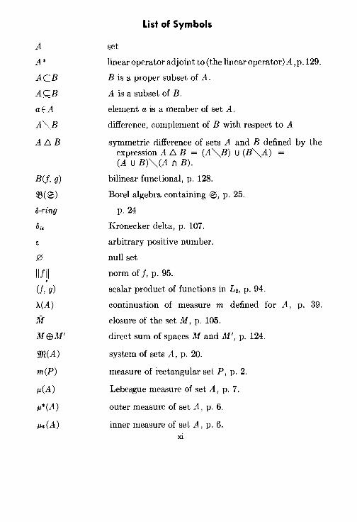
List of Symbols
set
linear operator adjoint to(the linearoperator)A ,p.129.
B is a proper subset of A.
A is a subset of B.
element a is a member of set A.
difference, complement of B with respect to A
symmetric difference of sets A and B defined by the expressionAL. B = (A~B) u (B~A) (A u B)~(A n B).
bilinear functional, p. 128.
Borel algebra containing ®, p. 25.
p. 24
Kronecker delta, p. 107.
arbitrary positive number.
null set
norm of j, p. 95 .
scalar product of functions in L2, p. 94.
continuation of measure m defined for A, p. 39.
closure of the set M, p. 105.
direct sum of spaces M and M', p. 124.
system of sets A, p. 20.
measure of rectangular set p' p. 2.
Lebesgue measure of set A, p. 7.
outer measure of set A, p. 6.
inner measure of set A, p. 6. xi
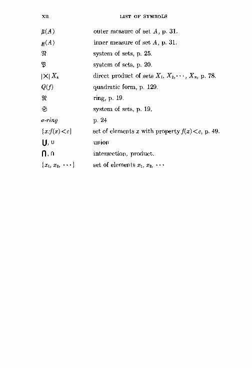
XII
p(A)
H(A)
SR
'l3 IXIXk
Q(f)
m ®
u-ring
{x:f(x)<c}
u, u
n,n
LIST OF SYMBOLS
outer measure of set A, p. 31.
inner measure of set A, p. 31.
system of sets, p. 25.
system of sets, p. 20.
direct product of sets X1, X2, · • ·, X n, p. 78.
quadratic form, p. 129.
ring, p. 19.
system of sets, p. 19.
p.24
set of elements x with property f(x)<c, p. 49.
union
intersection, product.
set of elements x1, x2, • • •
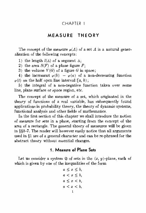
CHAPTER I
MEASURE THEORY
The concept of the measure ~(A) of a set A is a natural gener-alisation of the following concepts:
1) the length Z(ll) of a segment !l; 2) the area S(F) of a plane figure F; 3) the volume V(G) of a figure Gin space; 4) the increment cp(b) - cp(a) of a non-decreasing function
cp(t) on the half open line interval [a, b); 5) the integral of a non-negative function taken over some
line, plane surface or space region, etc.
The concept of the measure of a set, which originated in the theory of functions of a real variable, has subsequently found applications in probability theory, the theory of dynamic systems, functional analysis and other fields of mathematics.
In the first section of this chapter we shall introduce the notion of measure for sets in a plane, starting from the concept of the area of a rectangle. The general theory of measures will be given in §§3-7. The reader will however easily notice that all arguments used in §1 are of a general character and can be re-phrased for the abstract theory without essential changes.
1 . Measure of Plane Sets
Let us consider a system 10 of sets in the (x, y)-plane, each of which is given by one of the inequalities of the form
a::::;; x ::::;; b,
a< x::::;; b,
a::::;; x < b,
a< x < b, 1

2 I. MEASURE THEORY
together with one of the inequalities
c s y s d,
c < y s d,
c s y < d,
c < y < d,
where a, b, c and d are arbitrary numbers. The sets belonging to this system we shall call "rectangles". The closed rectangle, given by the inequalities
as x S b,
is the usual rectangle (including the boundary) if a < b and c < d, or a segment if a = b and c < d, or a point if a = b and c = d. The open rectangle
a< x < b, c<y<d
is, depending on the relations among a, b, c and d, respectively, a rectangle without boundaries, or the empty set. Each of the rectangles of the other types (let us call them half-open) is either a real rectangle without one, two or three sides, or an interval, or a half-interval, or, finally, an empty set.
We shall define for each of the rectangles a measure corresponding to the concept of area, well known from elementary geometry, in the following way:
a) the measure of an empty set is equal to zero; b) the measure of a non-empty rectangle (closed, open or
half-open) given by the numbers a, b, c and dis equal to
(b - a) (d - c).
In this way, to each rectangle P there correspo_nds a number m (P) -the measure of this rectangle; moreover the following conditions are obviously satisfied:
1) the measure m(P) takes on real non-negative values; n
2) the measure is additive, i.e., if P = U Pk and P; n Pk = 5Zf k=i

!. MEASURE OF PLANE SETS 3
for i ,e k, then m(P) = 't m(Pk).
k=l
Our task now is to generalise the measure m (P), which up to now has been defined only for rectangles, to a wider class of measures, preserving the properties 1) and 2).
The first step in this direction consists of generalising the concept of measure to so called elementary sets. We shall call a plane set elementary if it can be represented, at least in one way, as a union of a finite number of pairwise non-intersecting rectangles.
For what follows we shall use the following
Theorem 1. The union, intersection, difference and symmetric difference of two elementary sets is also an elementary set.
Proof. It is clear that the intersection of two rectangles is again a rectangle. Therefore, if
A = U Pk and B = U Q; k
are two elementary sets, then
A n B = U (Pk n Q;) k,i
is also an elementary set.
The difference of two rectangles is, as is easily checked, an elementary set. Hence, taking away from the rectangle some elementary set we again obtain an elementary set (as the intersection of elementary sets). Now let A and B be two elementary sets. One can obviously find a rectangle P containing each of them. Then
is an elementary set by what has been said above. From this and the equalities
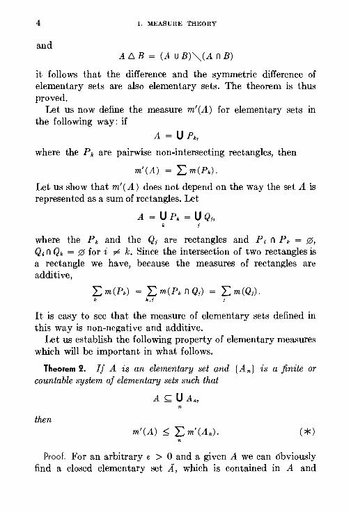
4 I. MEASURE THEORY
and A L. B = (A u B)"'-(A n B)
it follows that the difference and the symmetric difference of elementary sets are also elementary sets. The theorem is thus proved.
Let us now define the measure m'(A) for elementary sets in the following way: if
A = U Pk,
where the Pk are pairwise non-intersecting rectangles, then
m' (A) = L m(Pk).
Let us show that m' (A) does not depend on the way the set A is represented as a sum of rectangles. Let
A = U Pk = U Q;, k
where the Pk and the Q; are rectangles and P; n Pk = 0, Q;. n Qk = 0 for i ,e k. Since the intersection of two rectangles is a rectangle we have, because the measures of rectangles are additive,
'L m(Pk) = 'L m(Pk n Q;) = L m(Q;). k k,i i
It is easy to see that the measure of elementary sets defined in this way is non-negative and additive.
Let us establish the following property of elementary measures which will be important in what follows.
Theorem 2. If A is an elementary set and {An} is a finite or countable system of elementary sets such that
A~ U An,
then m'(A) ::::; L m'(An).
Proof. For an arbitrary e > 0 and a given A we can 6bviously find a closed elementary set A, which is contained in A and
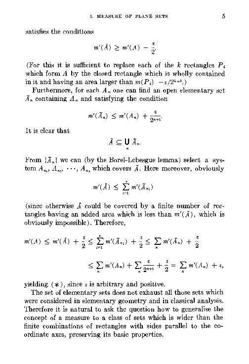
!. MEASURE OF PLANE SETS 5
satisfies the conditions
m'(A) ~ m'(A) e
(For this it is sufficient to replace each of the k rectangles P;. which form A by the closed rectangle which is wholly contained in it and having an area larger than m(P;) -e/2k+1.)
Furthermore, for each An one can find an open elementary set An containing An and satisfying the condition
It is clear that
From {An) we can (by the Borel-Lebesgue lemma) select a system Anu An,, ···,An. which covers A. Here moreover, obviously
m'(A) ::=; :t m'(AnJ i=l
(since otherwise A could be covered by a finite number of rectangles having an added area which is less than m'(A), which is obviously impossible). Therefore,
m'(A) ::=; m'(A) + ~ ::::; :t m'(A • .) + ~ < Ln m'(An) + -2e
2 i=l 2-
yielding ( *), since e is arbitrary and positive. The set of elementary sets does not exhaust all those sets which
were considered in elementary geometry and in classical analysis. Therefore it is natural to ask the question how to generalise the concept of a measure to a class of sets which is wider than the finite combinations of rectangles with sides parallel to the coordinate axes, preserving its basic properties.

6 I. MEASURE THEORY
The final solution of this problem was given by H. Lebesgue at the beginning of the twentieth century.
In presenting the theory of Lebesgue's measure we will have to consider not only finite but also infinite combinations of rectangles.
In order to avoid dealing with infinite values for measures we shall limit ourselves to sets which fully belong to the square E = {0 s X s 1; 0 s y s 1).
On the set of all these sets we shall define two functions ~*(A) and ~*(A) in the following way.
Definition 1. We shall call the number
inf 'L:m(Pk) A C:UPk
the outer measure ~*(A) of the set A; the lower bound is taken over all possible coverings of the set A by finite or countable rectangles.
Definition 2. We call the number
1- ~*(~A)
the inner measure ~*(A) of the set A. It is easy to see that always
~*(A) s ~*(A). Indeed, suppose that for some A C E
~*(A) >~*(A),
i.e.,
~*(A) + ~*(E""'A) < 1.
Then, by definition of the exact lower bound, one can find systems of rectangles {P;) and { Qk) covering A and E""'A, respectively, such that
The union of the systems {P;) and {Qk) we shall denote by
I. MEASURE OF PLANE SETS
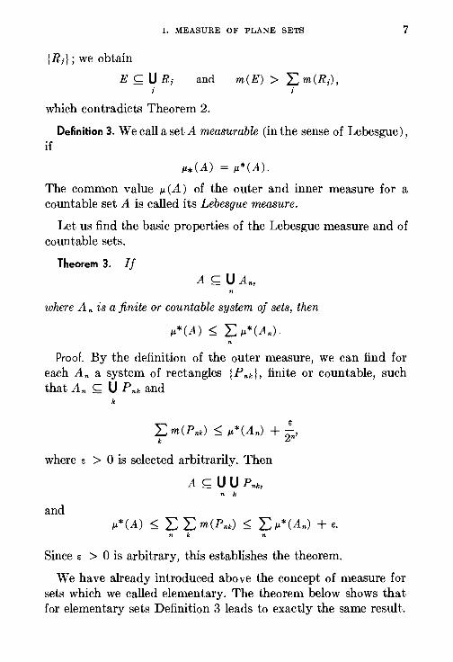
{Ri}; we obtain
E s;;;; U R; and
which contradicts Theorem 2.
m(E) > L m(R;), i
7
DeAnition 3. We call a set A measurable (in the sense of Lebesgue), if
~*(A) =~*(A).
The common value ~(A) of the outer and inner measure for a countable set A is called its Lebesgue measure.
Let us find the basic properties of the Lebesgue measure and of countable sets.
Theorem 3. If
where An is a finite or countable system of sets, then
~*(A) :::=; L ~*(An)·
Proof. By the definition of the outer measure, we can find for each An a system of rectangles { P nk), finite or countable, such that An ~ U Pnk and
k
t= m(Pnk) ::::; ~*(An) + ~'
where e > 0 is selected arbitrarily. Then
A~ U U Pnk, n k
and ~*(A) ::::; L L m(Pnk) ::::; L ~*(An) +e.
n k
Since e > 0 is arbitrary, this establishes the theorem.
We have already introduced above the concept of measure for sets which we called elementary. The theorem below shows that for elementary sets Definition 3 leads to exactly the same result.
8 I. MEASURE THEORY
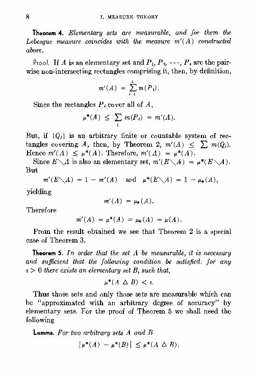
Theorem 4. Elementary sets are measurable, and for them the Lebesgue measure coincides with the measure m' (A) constructed above.
Proof. If A is an elementary set and P~, P2, · · ·, Pk are the pairwise non-intersecting rectangles comprising it, then, by definition,
k
m'(A) = 'L:m(P;). i=l
Since the rectangles P; cover all of A,
~*(A) ~ L: m(P;) = m'(A).
But, if { Qi) is an arbitrary finite or countable system of rectangles covering A, then, by Theorem 2, m'(A) ~ L: m(Qi). Hence m'(A) ~ ~*(A). Therefore, m'(A) = ~*(A).
Since E""'A is also an elementary set, m'(E""'A) = ~*(E""'A). But
m'(E""'A) = 1- m'(A) and ~*(E""'A) = 1 -~*(A),
yielding m'(A) = ~(A).
Therefore m'(A) =~*(A) =~*(A) =~(A).
From the result obtained we see that Theorem 2 is a special case of Theorem 3.
Theorem 5. In order that the set A be measurable, it is necessary and sufficient that the following condition be satisfied: for any e > 0 there exists an elementary set B, such that,
~*(A !:::. B) < e.
Thus those sets and only those sets are measurable which can be "approximated with an arbitrary degree of accuracy" by elementary sets. For the proof of Theorem 5 we shall need the following
Lemma. For two arbitrary sets A and B
I ~*(A) -~*(B) I ~ ~*(A !:::. B).
l. MEASURE OF PLANE SETS 9
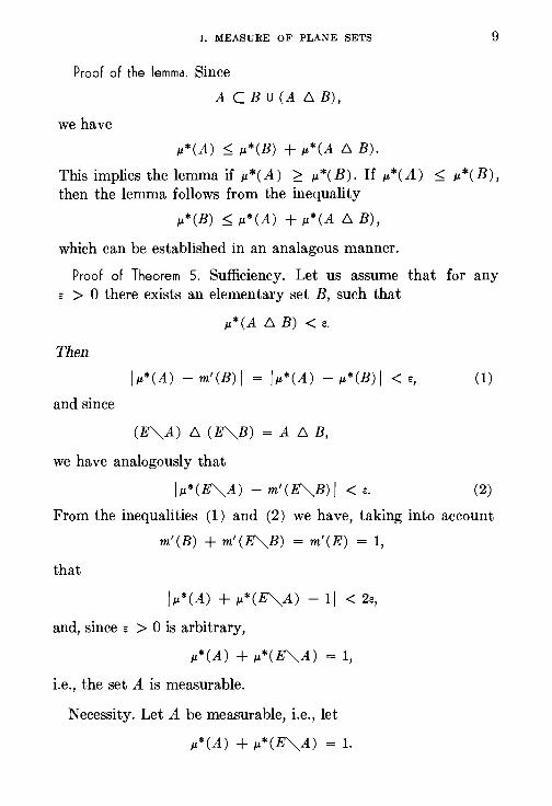
Proof of the lemma. Since
A C B u (A !:::. B),
we have
~*(A) ~ ~*(B) +~*(A !:::. B).
This implies the lemma if ~*(A) ~ ~*(B). If ~*(A) ~ ~*(B), then the lemma follows from the inequality
~*(B) ~ ~*(A) +~*(A !:::. B),
which can be established in an analagous manner.
Proof of Theorem 5. Sufficiency. Let us assume that for any e > 0 there exists an elementary set B, such that
~*(A !:::. B) < e.
Then
/~*(A) -m'(B)/ /~*(A) -~*(B)/ < e, (1)
and since
we have analogously that
/~*(E"'-A) - m'(E"'-B) / <e. (2)
From the inequalities (1) and (2) we have, taking into account
m'(B) + m'(E"'-B) = m'(E) = 1,
that
/~*(A) + ~*(~A) - 1/ < 2e,
and, since e > 0 is arbitrary,
i.e., the set A is measurable.
Necessity. Let A be measurable, i.e., let
~*(A) +~*(~A) = 1.
10 I. MEASURE THEORY
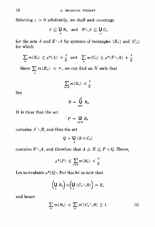
Selecting e > 0 arbitrarily, we shall seek coverings
A ~ U Bn and E"A ~ U Cn n n
for the sets A and E""'A by systems of rectangles {Bn} and {Cn) for which
~ e ~ e ~ m(Bn) ~ ~*(A) + 3 and ~ m(Cn) ~ ~*(E""'A) + 3·
Since L: m (Bn) < oo, we can find an N such that
L m(Bn) < 3~. n>N
Set N
B = U Bn. n=l
It is clear that the set
P = U Bn n>N
contains A ""'B, and that the set
Q = U (B n Cn) n
contains B""'A, and therefore that A !:::. B s:;;; P u Q. Hence,
~*(P) ~ L m(Bn) < -3e.
n>N
Let us evaluate~*( Q). For this let us note that
and hence
L m(Bn) + L m'(Cn""'B) ~ 1. (3) n
I. MEASURE OF PLANE SETS 11
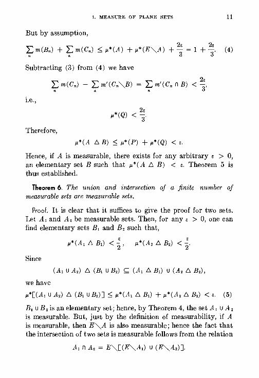
But by assumption,
2a 2e L m(Bn) + L m(Cn) s ~*(A) + ~*(E"'-A) +- = 1 + -. (4) n n 3 3
Subtracting (3) from (4) we have
i.e.,
Therefore,
2e L m'(Cn n B) < 3'
2a ~*(Q) < 3'
~*(A !:::. B) s ~*(P) + ~*(Q) < e.
Hence, if A is measurable, there exists for any arbitrary e > 0, an elementary set B such that ~*(A D. B) < e. Theorem 5 is thus established.
Theorem 6. The union and intersection of a finite number of measurable sets are measurable sets.
Proof. It is clear that it suffices to give the proof for two sets. Let A1 and A2 be measurable sets. Then, for any e > 0, one can find elementary sets B1 and B2 such that,
Since
we have
B1 u B 2 is an elementary set; hence, by Theorem 4, the set A 1 u A 2
is measurable. But, just by the definition of measurability, if A is measurable, then E"'-A is also measurable; hence the fact that the intersection of two sets is measurable follows from the relation
12 I. MEASURE THEORY
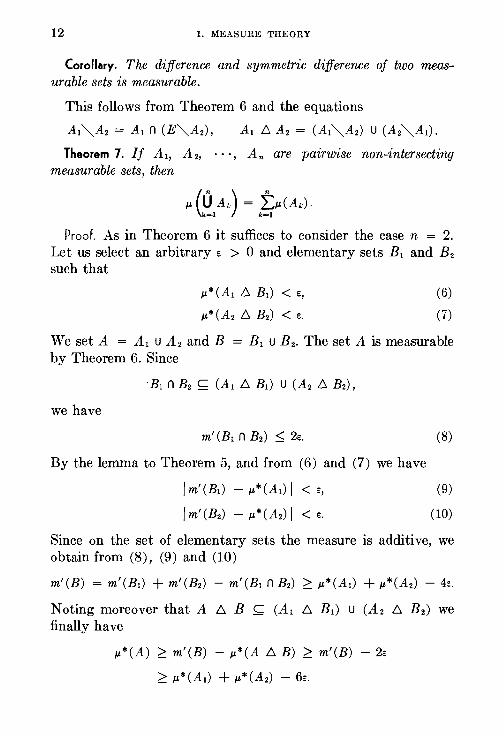
Corollary. The difference and symmetric difference of two measurable sets is measurable.
This follows from Theorem 6 and the equations
A1"'A2 = A1 n (E"'A2), A1 D. A2 = (A1"'A2) u (A2"'A1).
Theorem 7. If A1, A2, · · ·, An are pairwise non-intersecting measurable sets, then
Proof. As in Theorem 6 it suffices to consider the case n = 2. Let us select an arbitrary e > 0 and elementary sets B1 and B2 such that
~*(AI D. B1) < e,
~* (A2 D. B2) < e.
(6)
(7)
We set A = A1 u A2 and B = B1 u B2. The set A is measurable by Theorem 6. Since
·B1 n B2 ~ (A1!:::. B1) U (A2 D. B2),
we have
m' (B1 n B2) ::::;; 2e.
By the lemma to Theorem 5, and from (6) and (7) we have
/m'(BI)- ~*(AI)/< e,
/m'(B2) - ~*(A2) / <e.
(8)
(9)
(10)
Since on the set of elementary sets the measure is additive, we obtain from (8), (9) and (10)
m'(B) = m'(B1) + m'(B2) - m'(B1 n B2) ~ ~*(A1) + ~*(A2) - 4<.
Noting moreover that A !:::. B s:;;; (A1 !:::. B1) u (A2 !:::. B2) we finally have
~*(A) ~ m'(B) - ~*(A !:::. B) ~ m'(B) - 2e
~ ~*(AI) + ~*(A2) - 6e.
I. MEASURE OF PLANE SETS
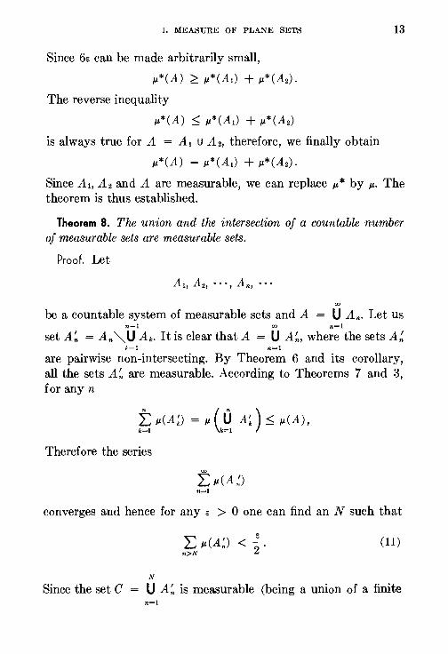
Since 6e can be made arbitrarily small,
~*(A) ~ ~*(AI) + ~*(A2). The reverse inequality
~*(A) ::::;; ~*(AI) + ~*(A2) is always true for A = A1 u A2, therefore, we finally obtain
~*(A) = ~*(AI) + ~*(A2).
13
Since A1, A2 and A are measurable, we can replace ~*by~· The theorem is thus established.
Theorem 8. The union and the intersection of a countable number of measurable sets are measurable sets.
Proof. Let
ro
be a countable system of measurable sets and A U An. Let US n-1 oo n=l
set A~ = An""' U Ak. It is clear that A = U A~, where the sets A~ k=l n=l
are pairwise non-intersecting. By Theorem 6 and its corollary, all the sets A~ are measurable. According to Theorems 7 and 3, for any n
Therefore the series
n=i
converges and hence for any e > 0 one can find an N such that
L ~(A~) < _2e • n>N
(11)
N
Since the set C U A~ is measurable (being a union of a finite n=l
14 I. MEASURE THEORY
number of measurable sets), we can find an elementary set B such that
e J.L*(C!:::. B) < "2. (12)
Since
A !:::. B ~ ( C !:::. B) u ( U A~) , n>N
(11) and (12) yield
J.L*(A !:::. B) < e.
Because of Theorem 5 this implies that the set A is measurable. Since the complement of a measurable set is itself measurable,
the statement of the theorem concerning intersections follows from the equality
Theorem 8 is a generalisation of Theorem 6. The following Theorem is a corresponding generalisation of Theorem 7.
Theorem 9. If {An) is a sequence of pairwise non-intersecting measurable sets, and A = U An, then
n
Proof. By Theorem 7, for any N,
J.L(Q1 An)= ~J.L(An) s J.L(A).
Taking the limit as N ---> oo, we have
(13) n=l
On the other hand, according to Theorem 3,
(14) n=l
Inequalities (13) and (14) yield the assertion of the Theorem.
I. MEASURE OF PLANE SETS 15
The property of measures established in Theorem 9 is called its countable additivity, or u-additivity. An immediate corollary of u-additivity is the following property of measures, called continuity.
Theorem 10. If A1 :;2 A2 ;:2 • • • is a sequence of measurable sets, contained in each other, and A = 0 An, then
~(A) = lim ~(An).
It suffices, obviously, to consider the case A = 5Zf, since the general case can be reduced to it by replacing An by An ""A. Then
A1 = (A1""A2) u CA2""Aa) u · · ·
and
Therefore
~(A1) f: ~(Ak""Ak+I), (15) k=i
and
(16) k=n
since the series (15) converges, its remainder term (16) tends to zero as n --> oo. Thus,
~(An) --> 0 for n--> oo,
which was to be shown.
Corollary. If A1 ~ A 2 ~ • • • is an increasing sequence of measurable sets, and
then
~(A) = lim ~(An).
16 I. MEASURE THEORY
For the proof it suffices to go over from the sets An to their complements and to use Theorem 10.
Thus we have generalised the concept of a measure from elementary sets to a wider class of sets, called measurable sets, which are closed with respect to the operations of countable unions and intersections. The measure constructed is u-additive on this class of sets.
Let us make a few final remarks.
1. The theorems we have derived allow us to obtain an idea of the set of all Lebesgue measurable sets.
Since every open set belonging to E can be represented as a union of a finite or countable number of open rectangles, i.e., measurable sets, Theorem 8 implies that all open sets are measurable. Closed sets are complements of open sets and consequently are also measurable. According to Theorem 8 also all those sets must be measurable which can be obtained from open or closed sets by a finite or countable number of operations of countable unions and intersections. One can show, however, that these sets do not exhaust the set of all Lebesgue measurable sets.
2. We have considered above only those plane sets which are subsets of the unit square E = { 0 ::::;; x, y ::::;; 1). It is not difficult to remove this restriction, e.g., by the following method. Representing the whole plane as a sum of squares E,m = {n ::::;; x ::::;; n + 1, m ::::;; y ::::;; m + 1) (m, n integers), we shall say that the plane set A is measurable if its intersection Anm = A n Enm with each of these squares is measurable, and if the series L: p.( Anm) converges. Here we assume by definition that n,m
p.(A) = L p.(Anm). n,m
All the properties of measures established above can obviously be carried over to this case.
3. In this section we have given the construction of Lebesgue measures for plane sets. Analogously Lebesgue measures may be constructed on a line, in a space of three dimensions or, in general, in a space of n dimensions. In each of these cases the measure is constructed by the same method: proceeding from a measure de-
I. MEASURE OF PLANE SETS 17
fined earlier for some system of simple sets (rectangles in the case of a plane, intervals (a, b), segments [a, b] and half-lines (a, b] and [a, b) in the case of a line, etc.) we first define a measure for finite unions of such sets, and then generalise it to a much wider class of sets-to sets which are Lebesgue measurable. The definition of measurability itself can be carried over word for word to sets in spaces of any dimension.
4. Introducing the concept of the Lebesgue measure we started from the usual definition of an area. The analogous construction for one dimension is based on the concept of length of an interval (segment, half-line). One can however introduce measure by a different and more general method.
Let F(t) be some non-decreasing function, continuous from the left, and defined on a line. We set
m(a, b) = F(b) - F(a + O),
m[a, b] = F(b + 0) - F(a),
m(a, b] = F(b + O) - F(a + 0),
m[a, b) = F(b) - F(a).
It is easy to see that the function of the interval m defined in this way is non-negative and additive. Applying to it considerations which are analogous to the ones used in this section, we can construct some measure J.LF( A). Here the set of sets, which are measurable with respect to the given measure, is closed with respect to the operations of countable unions and intersections, and the measure J.LF is u-additive. The class of sets, measurable with respect to J.LF, will, generally speaking, depend on the choice of the function F. However, for any choice of F, the open and closed sets, and therefore all their countable unions and intersections will obviously be measurable. Measures obtained from some function F are called Lebesgue-Stieltjes measures. In particular, to the function F( t) = t there corresponds the usual Lebesgue measure on a line.
If the measure J.LF is such that it is equal to zero for any set whose normal Lebesgue measure is zero, then the measure J.LF is called completely continuous. If the measure is wholly concen-
18 I. MEASURE THEORY
trated on a finite or countable set of points (this happens when the set of values of the function F(t) is finite or countable), then it is called discrete. The measure J.LF is called singular, if it is equal to zero for any one point set, and if there exists such a set M with Lebesgue measure zero, that the measure J.LF of its complement is equal to zero.
One can show that any measure J.LF can be represented as a sum of an absolutely continuous, a discrete and a singular measure.
Existence of Non-measurable Sets
It has been shown above that the class of Lebesgue measurable sets is quite wide. Naturally the question arises as to whether there exist any non-measurable sets at all. We shall show that this problem is solved affirmatively. It is easiest to construct non-measurable sets on a circle.
Consider a circle with circumference C of unit length and let a be some irrational number. Let us consider those points of the circumference C which can be transformed into each other by a rotation of the circle through an angle na ( n an integer) as belonging to our class. Each of these classes will obviously consist of a countable number of points. Let us now select from each of these classes one point. We shall show that the set obtained in this manner, let us call it <1>, is non-measurable. Let us call the set, obtained from <I> by a rotation through angle na, <I>n. It is easily seen that all the sets <I>n are pairwise nonintersecting, and that they add up to the whole circular arc C. If the set <I> were measurable, then the sets <I>n, congruent to it, would also be measurable. Since
C = 0 <I>n, <I>n n <I>m = 5Zf for n ,e m,
this would imply, on the strength of the u-additivity of measures that,
(17)
But congruent sets must have the same measure:
This shows that equation (17) is impossible, since the sum of the series on the right-hand side of equation (17) is equal to zero if J.L(<I>) = 0, and is infinite if J.L(<I>) > 0. Thus the set <I> (and hence also each <I>n) is non-measurable.
2. SYSTEMS OF SETS 19
2. Systems of Sets
Before proceeding to the general theory of sets we shall first give some information concerning systems of sets, which supplements the elements of set theory discussed in Chapter I of Volume I.
We shall call any set, the elements of which are again certain sets, a system of sets. As a rule we shall consider systems of sets, each of which is a subset of some fixed set X. We shall usually denote systems of sets by Gothic letters. Of basic interest to us will be systems of sets satisfying, with respect to the operations introduced in Chapter I, §1 of Volume I, certain definite conditions of closure.
Definition 1. A non-empty system of sets m is called a ring if it satisfies the conditions that' A E m and B E m implies that the sets A !:::. B and A n B belong to m.
For any A and B
A u B = (A !:::. B) !:::. (A n B), and
A"'-B = A !:::. (A n B);
he.nce A E m and B E m also imply that the sets A u B and A "'-B belong to m. Thus a ring of sets is a system which is invariant with respect to the operations of union and intersection, subtraction and the formation of a symmetric difference. Obviously the ring is also invariant with respect to the formation of any finite number of unions and intersections of the form
k=l
Any ring contains the empty set fZf, since always A "'-A = fZf. The system consisting of only the empty set is the smallest possible ring of sets.
A set E is called the unit of the system of sets 0, if it belongs to 0 and if, for any A E 0, the equation
An E =A holds.
20 I. MEASURE THEORY
Hence the unit of the system of sets ~ is simply the maximal set of this system, containing all other sets which belong to ~.
A ring of sets with a unit is called an algebra of sets.
Examples. 1) For any set A the system 9R (A) of all its subsets is an algebra of sets with the unit E = A.
2) For any non-empty set A the system { fZf, A) consisting of the set A and the empty set fZf, forms an algebra of sets with the unitE =A.
3) The system of all finite subsets of an arbitrary set A forms a ring of sets. This ring is then and only then an algebra if the set A itself is finite.
4) The system of all bounded subsets of the line forms a ring of sets which does not contain .a unit.
From the definition of a ring of sets there immediately follows
Theorem 1. The intersection m = 0 ma of any set of rings is also a ring.
Let us establish the following simple result which will however be important in the subsequent work.
Theorem 2. For any non-empty system of sets ~ there exists one and only one ring m ( ~), containing ~ and contained in an arbitrary ring m which contains ~.
Proof. It is easy to see that the ring m ( ~) is uniquely defined by the system ~. To prove its existence let us consider the union X = U A of all sets A contained in ~ and the ring 9R (X) of all
A•;o
subsets of the set X. Let ~be the set of all rings of sets contained in 9R (X) and containing ~. The intersection
of all these rings will obviously be the required ring m ( ~).
2. SYSTEMS OF SETS 21
Indeed, whatever the ffi* containing ~. the intersection ffi = ffi* n 9R (X) is a ring of ~ and, therefore,
~ s;;;; ll3 ~ m s;;;; m*, i.e., ll3 really satisfies the requirement of being minimal. ffi ( ~) is called the minimal ring over the system ®.
The actual construction of the ring ffi(~) for a given system~ is, generally speaking, fairly complicated. However, it becomes quite straightforward in the important special case when the system ~ is a "semiring".
Definition 2. A system of sets ~ is called a semiring if it contains the empty set, is closed with respect to the operation of intersection, and has the property that if A and A1 s;;;; A belong to ~.
n
then A can be represented in the form A = U Ak, where the Ak k=l
are pairwise non-intersecting sets of ~. the first of which is the given set A1.
In the following pages we shall call each system of non-intersecting sets A1, A2, · · ·, An, the union of which is the given set A, a finite decomposition of the set A.
Every ring of sets ffi is a semiring since if A and A 1 s;;;; A belong to m, then the decomposition
A = A1 u A2,
where
takes place. As an example of a semiring which is not a ring of sets we can
take the set of all intervals (a, b), segments [a, b] and half segments (a, b] and [a, b) on the.real axis.*
In order to find out how the ring of sets which is minimal over a given semiring is constructed, let us establish some properties of semirings of sets.
* Here, of course, the intervals include the" empty" interval (a, a) and the segments consisting of one point [a, a].

22 I. MEASURE THEORY
Lemma 1. Let the sets A1, A 2, · · ·, An, A belong to the semiring ~' and let the sets A; be pairwise non-intersecting and be subsets of the set A. Then, the sets A; ( i = 1, 2, · · ·, n) can be included as the first n members of the finite decomposition
s ~ n,
of the set A, where all the Ak E ~.
Proof. The proof will be given by induction. For n = 1 the statement of the lemma follows from the definition of a semiring. Let us assume that the result is true for n = m and let us consider m + 1 sets A1, A 2, • • ·, Am, Am+1 satisfying the conditions of the lemma. By the assumptions made,
A = A1 u A2 u · • · u Am u B1 u B2 u · · · u Bp,
where the sets Bq ( q = 1, 2, · · ·, p) belong to ~. Set
By the definition of a semiring, we have the decomposition
Bq = Bq1 u Bq2 u · · • u Bqr.,
where all the Bqi belong to ~. It is easy to see that
P rq A = A1 u • · · u Am u Am+1 u U U Bqi·
q-1 i-2
Thus the assertion of the lemma is proved for n = m + 1, and hence for all n.
Lemma 2. Whatever the finite system of sets A 1, A 2, • • ·, An belonging to the semiring may be, one can find in ~ a finite system of pairwise non-intersecting sets B 1, B 2, • • • , B 1 such that each A k can be represented as a union
of some of the sets B •.
Proof. For n = 1 the lemma is trivial since it suffices to set t = 1, B1 = A1. Assume that it is true for n = m and consider
2. SYSTEMS OF SETS 23
in~ some system of sets A1, A2, • • ·, Am+l· Let B1, B2, • · ·, B 1 be sets from ~' satisfying the conditions of the lemma with respect to A1, A2, ···,Am. Let us set
By Lemma 1, we have the decomposition t q
Am+l = U B.1 u U Bp', Bp' E ®, (1) s=l p=l
and by the definition of the semiring itself we have the decomposition
B. = B.1 u B.2 u • • • u B.1,, B,q E ~.
It is easy to see that
'· Ak = U U B,q, k = 1, 2, · · ·, m, 8€.~k q=l
and that the sets
B' p
are pairwise non-intersecting. Thus the sets B,q, B/ satisfy the conditions of the lemma with respect to A1, A 2, • • ·, Am, Am+l· The lemma is thus proved.
Theorem 3. If ~ is a semi ring, then m ( ~) coincides with the system 13 of the sets A, which admit of the finite decompositions
n
A= U Ak k=l
into the sets Ak E ~.
Proof. Let us show that the system 13 forms a ring. If A and B are two arbitrary sets in 13, the decompositions
m
B = U Bk, k=l
take place. Since ~ is a semiring, the sets
C;; =A, n B;
24 I. MEASURE THEORY
also belong to ~. By Lemma 1 we have the decompositions
A; = U C ;; u U D ;k, i k-1
•;
B; = U C;; u U E;k, . i k-1
(2)
where D;k, Eik E ~. From equation (2) it follows that the sets A n Band A!:::. B admit of the decompositions
A n B = U C;11 i.i
A !:::. B = U D;k u U E;k, i,k i.k
and therefore belong to ,8. Hence, 13 is indeed a ring; the fact that it is minimal among all the rings containing ~ is obvious.
In various problems, in particular in measure theory, one has to consider unions and intersections of not only finite, but aL<;o infinite numbers of sets. Therefore it is useful to introduce, in addition to the concept of a ring of sets, the following concepts.
Definition 3. A ring of sets is called au-ring, if with each sequence of sets A1, A 2, • • ·, An, • • · it also contains the union
S = U An•
Definition 4. A ring of sets is called a 8-ring, if in addition to each sequence of sets A1, A2, · • ·, An, · · • it also contains the intersection
D = 0 An. n
It is natural to call a u-ring with a unit a u-algebra, and a 8-ring with a unit a 8-algebra. However, it is easy to see that these two concepts coincide: each u-algebra is at the same time a 8-algebra, and each 8-algebra is a u-algebra. This follows from the duality relations
U An = E""O ( E""An), n n
(see Chapter 1, §1 of Volume 1). The 8-algebras, or what is the
2. SYSTEMS OF SETS 25
same thing, the u-algebras, are usually called Borel algebras, or simply B-algebras.
The simplest example of a B-algebra is the set of all subsets of some set A.
A theorem, analogous to Theorem 2 proved above for rings, holds for B-algebras.
Theorem 4. For any non-empty system of sets ® there exists a B-algebra 58 ( ®), containing ® and contained in any B-algebra which contains ®.
The proof follows exactly the same lines as does the proof of Theorem 2. The B-algebra 58 ( ®) is called the minimal B-algebra over the system ® or the Borel closure of the system ®.
So called Borel sets orB-sets play an important role in analysis. These sets can be defined as sets on the real axis belonging to the minimal B-algebra over the set of all segments [a, b ].
As a supplement to the information given in Chapter 1, §7 of Volume I, let us note the following facts which we shall need in Chapter II.
Let y = f( x) be a function defined on the set M with values from the set N. Let us denote the system of all maps f( A) of sets from the system 9R (we assume that 9R consists of subsets of the set M) by f( 9R) and the system of all subimages f- 1(A) of sets from 91 (we assume that 91 consists of subsets of the set N) by f- 1(91). The following statements are true:
1) If 91 is a ring, then f-1( 91) is a ring.
2) If 91 is an algebra, then r 1( 91) is an algebra.
3) If 91 is a B-algebra, then f-1( 91) is a B-algebra.
'4) m u-1 c 91)) = f-1c me 91)). s) 58 u-1 (91)) = f-1c 58(91) ).
Let m be some ring of sets. If in it we take the operation A !:::. B to be "addition" and A n B to be "multiplication", then m is a ring in the usual algebraic sense of the word. All its elements will satisfy the conditions
a+ a= 0, a2 =a.
26 I. MEASURE THEORY
Rings whose elements satisfy condition ( *) are called "Boolian" rings. Each Boolian ring can be realised as a ring of sets with the operations A !:::. Band A n B (Stone).
3. Measures on Semirings. Continuation of a Measure from a
Semiring to the Minimal Ring over it
In §1, when considering measure in the plane, we started from the measure of a rectangle (area) and then extended the concept of measure to a wider class of sets. The results as well as the methods given in §1 have a quite general character and can be generalized to measures defined on arbitrary sets without essential changes. The first step in constructing a measure on a plane consisted in generalizing the concept of measure from rectangles to elementary sets, i.e., to finite systems of pairwise non-intersecting rectangles.
In this section we shall consider the abstract analogue of this problem.
Definition 1. The set function p.( A) is called a measure if:
1) its domain of definition Sp. is a smniring of sets;
2) its values are real and non-negative;
3) it is additive, i.e., for any finite decomposition
A= U Ak
of the set A E S ~' into sets Ak E S ~'' the equation
p.(A) = LP.(Ak) holds.
Remark. From the decomposition 5Zf = 5Zf u 5Zf it follows that p.( 5Zf) = 2p.( 5Zf), i.e., p.( 5Zf) = 0.
The following two theorems about measures on smnirings will be frequently used in the subsequent pages.
Theorem 1. Let p. be a measure defined on some semiring S p.· If the sets A1, A2, ···,An, A belong to Sp., where the Ak are pairwise non-
3. MEASURES ON SEMIRINGS 27
intersecting and all belong to A, then
n
L~(Ak) ~~(A). k-1
Proof. Since S~' is a semiring there exists, according to Lemma 1, §2, the decomposition
. A = U Ak, s ~ n,
k=1
where the first n sets coincide with the given sets A1, A 2, • • ·, An. Since the measure of any set is non-negative,
n s
L:~(Ak) ~ L~(Ak) =~(A). k=1 k=1
Theorem 2. If A 1, A 2, • • ·, An, A belong to S p. and A s; U Ak, then k=1
" ~(A) ~ L ~(Ak). k=1
Proof. By Lemma 2, §2, one can find a system of pairwise nonintersecting sets B1, B2, · · ·, B 1 from Sp., such that each of the sets A 1, A 2, • • ·, A,., A can be represented as a union of some of the sets B.:
A= U B., k = 1, 2, · · ·, n. s€.lfo
Moreover, each index s E M0 also belongs to some member of M k· Therefore each term of the sum
L ~(B.) = ~(A) sE:..l/0
enters once, or at most a few times, into the double sum
n n
L L ~(B.) = L ~(Ak). k=1 ••Mk k=1
28 I. MEASURE THEORY
This yields n
~(A) s L~(Ak). k=l
In particular, for n = 1, we have the
Corollary. If A ~A', then ~(A) s ~(A'). Definition 2. The measure ~(A) is called the continuation of the
measure m(A) if Sm ~ S~' and if, for every A E Sm, the equality
~(A) = m(A)
holds.
The main aim of the present section is the proof of the following proposition.
Theorem 3. Every measure m( A) has one and only one continuation ~(A), having as its domain of definition the ring m (Sm).
Proof. For each set A E m (Sm) there exists a decomposition
(1)
(Theorem 3, §2). Let us assume by definition
n
~(A) = L m(Bk). (2) k=l
It is easy to see that the quantity ~(A), given by equation (2), does not depend on the selection of the decomposition (1). Indeed, let us consider the two decompositions
A = U B; = lJ C;, i=l i=l
Since all intersections B; n Cj belong to Sm, we have, because of the additivity of measures,
m n
L: m(B;) = L: L: m(B; n C;) L: m(C;), i=l i=l
4. CONTINUATIONS OF JORDAN MEASURES 29
which was to be proved. The fact that the function J.L( A), given by equation (2) is non-negative and additive is obvious. Hence the existence of a continuation J.L( A) of the measure m( A) is shown. To show its uniqueness let us note that, by definition of
n
continuation, if A = U Bk, where Bk are non-intersecting sets k=l
from Sm, then for any continuation J.L* of the measure m onto the ring ffi (Sm)
J.L*(A) = L J.L*(Bk) = L m(Bk) = J.L(A),
i.e., the measure J.L* coincides with the measure J.L defined by equation (2). The theorem is proved.
The connection between this theorem and the constructions of §1 will be completely clear if we note that the set of rectangles in the plane is a semiring, the area of these rectangles is a measure in the sense of Definition 1, and the elementary plane sets form a minimal ring over the semiring of the rectangles.
4. Continuations of Jordan Measures*
In the present section we shall consider the general form of that process which in the case of plane figures allows one to generalise from the definition of areas for a finite union of rectangles, with sides parallel to the axes of coordinates, to areas of all those figures for which areas are defined by elementary geometry or classical analysis. This extension was given with complete precision by the French mathematician Jordan around 1880. The basic idea of Jordan goes back, incidentally, to the mathematicians of ancient Greece and consists of approximating from the inside and from the outside the "measurable" set A by sets A' and A" to which a measure has already been prescribed, i.e., in such a way that the inclusions
A'~ A~ A"
are fulfilled.
• The concept of a Jordan measure has a definite historical and methodological interest but is not used in this exposition. The reader may omit this section if he wishes.
30 I. MEASURE THEORY
Since we can continue any measure onto a ring (Theorem 3, §3 ), it is natural to assume that the initial measure m be defined on a ring ffi = ffi (Sm). This assumption will be used during the whole of the present section.
DeAnition 1. We shall call a set A Jordan measurable if, for any e > 0, there exist in the ring ffi sets A' and A" which satisfy the conditions
A's;;;; A~ A",
Theorem 1. The system ffi* of Jordan measurable sets is a ring.
Indeed, let A E ffi *, B E= ffi *; then, for any e > 0, there exist A', A", B', B" E ffi such that
and
Hence
Since
we have
A' s;;;; A s;;;; A", B' ~ B s;;;; B",
A' u B' s;;;; A u B s;;;; A" u B", (1)
(2)
m[ (A" u B") "'-(A' u B')] :::; m[ (A'~A') u (B""'-B')]
:::; m(A'~A') + m(B""'-B') < ~ + ~ = e. (3)
Since
we have
e e :::; m(A""'-A') + m(B'~B') :::; 2 + 2 =e. (4)
4. CONTINUATIONS OF JORDAN MEASURES 31
Since e > 0 is arbitrary, and the sets A' u B', A" u B", A'""'B" and A"""'B' belong to ffi, (1), (2), (3) and (4) imply that A u B and A ""'B belong to ffi*.
Let 9R be a system of those sets A for which the set B :::2 A of ffi exists. For any A from 9R we set, by definition,
.U(A) = inf m(B), B~A
~(A) =supm(B). B.E.A
The functions .U( A) and ~(A) are called, respectively, the "outer" and the "inner" measure of the set A.
Obviously, always
~(A) ::; .a(A).
Theorem 2. The ring ffi* coincides with the system of those sets A E 9R for which ~(A) = .a( A).
Proof. If .a(A) -.e ~(A),
then
.U(A) - tt(A) = h > 0,
and for any A' and A" from ffi for which A' S::::: A S::::: A",
m(A') ::; tt(A), m(A") ~ .a(A),
m(A"""'A') = m(A") - m(A') ~ h > 0,
i.e., A cannot belong to ffi*. Conversely, if
~(A) = .a(A),
then, for any e > 0, there exist A' and A" from ffi for which
A's;;; A s;;; A",
e ~(A) - m(A') < 2,
e m(A") - .a(A) < 2,
m(A"""'A') = m(A") - m(A') < e,
32 I. MEASURE THEORY
i.e., A E ffi*.
The following theorems hold for sets from 'JR.
n
Theorem 3. If A s;;;; U Ak, then ,a(A) s L: ,a(Ak). k=l k=l
Proof. Let us select A/ such that
and let us form A' U A/. Then, k=l
m(A') S :t m(Ak') S :t ,a(Ak) + e, n
,a(A) s L ,a(Ak) + <, k=l k=l k=l
and since e is arbitrary, ,u(A) s L: ,a(A/). k=l
Theorem 4. If Ak s;;;; A (k = 1, 2, · · ·, n) and A; n Ai = fZf, then
~(A) ~ :t ~(Ak). k=l
Proof. Let us select Ak' s;;;; Ak such that
n
and let us form A' U Ak'· Then A/ n A/ 5Zf and k=l
n
m(A') = L: m(Ak') > L: ~(Ak) +e. k=l k
Since A' s;;;; A,
n
~(A) ~ m(A') ~ L ~(Ak) - e. k=l
4. CONTINUATIONS OF JORDAN MEASURES 33
Because e > 9 is arbitrary, n
~(A) ~ L~(Ak).
Let us now define the function J.L with the domain of definition
sp. = ffi*
as the common value of the inner and outer measures:
J.L(A) = ~(A) = JL(A).
Theorems 3 and 4, and the obvious fact that for A E ffi
JL(A) = ~(A) = m(A),
imply
Theorem 5. The function J.L( A) is a measure and a continuation of the measure m.
The construction given can be used for any measure m defined on a ring.
The system Sm 2 = ~of elementary sets in a plane is essentially connected with the coordinate system: the sets of the system ~ consist of rectangles with sides which are parallel to the coordinate axes. In going over to the Jordan measure
J<2l = j(m2)
this dependence on the choice of a coordinate system disappears: starting from an arbitrary system of coordinates jx1, x2} connected with the initial system { x1, x2} by the orthogonal transformation
X1 = COS a·X1 +sin a·X2 + a1,
X2 = -sin a·X1 +COS a·X2 + a2,
we obtain the same Jordan measure
J = j(m2) = j(m2)
(here m2 denotes the measure constructed with the help of rectangles with sides parallel to the axes x1, ~). This fact can be proved with the help of the following general theorem:
Theorem 6. In order that the Jordan continuations J.L1 = j(mt) and
J.l.2 = j(m2) of the measures m1 and m2 defined on the rings ffi1 and
34 I. MEASURE THEORY
ffi 2 coincide, it is necessary and sufficient that the following conditions be satisfied :
m1(A) = ~2(A) on ffi1,
m2(A) = ~1(A) on ffi2.
The necessity of the condition is obvious. Let us prove their sufficiency.
Let A E Sp.1
• Then there exist A', A" E Smp such that
A's;;;; A ~A", ") ') e m1(A - m1(A < 3'
and m1(A') ~ ~1(A) ~ m1(A").
Bytheconditionsofthetheorem, ~ 2 (A') = m1(A')and~2(A") m1(A").
From the definition of the measure ~2 it follows that there exist B' E Sm, and B" E 8m 2 for which,
A' 2 B' and
B" 2 A" and m2(B") - ~2(A") < ~·
Here B' ~A s;;;; B",
and, obviously,
m2(B") - m2(B') < e.
Since e > 0 is arbitrary, A E S ~'•' and from the relations
~1(B') = m2(B') s ~2(A) ~ m2(B") = ~1(B")
it follows that
~2(A) = ~1(A).
The theorem is proved. To establish that the Jordan measure in the plane is inde
pendent of the choice of the system of coordinates, one need only
5. COUNTABLE ADDITIVITY 35
convince oneself that a set which is obtained from an elementary set by a rotation through some angle a is Jordan measurable. It is suggested that the reader do this for himself.
If the initial measure is given, not on a ring, but on a semiring, then it is natural to consider as its Jordan continuation the measure
j(m) = j(r(m)),
obtained as a result of a continuation of m to the ring ffi (Sm) and a subsequent continuation.
5. Countable Additivity. General Problem of Continuation
of Measures
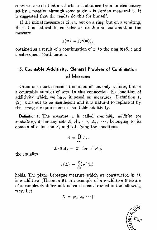
Often one must consider the union of not only a finite, but of a countable number of sets. In this connection the condition of additivity which we have imposed on measures (Definition 1, §2) turns out to be insufficient and it is natural to replace it by the stronger requirement of countable additivity.
Definition 1. The measure J.L is called countably additive (or u-additive), if, for any sets A, A1, ···,An, ···,belonging to its domain of definition Sp. and satisfying the conditions
A; n A; = 5Zf for i ,e j,
the equality
J.L(A) = f: J.L(An) n-1
holds. The plane Lebesgue measure which we constructed in §1 is u-additive (Theorem 9 ). An example of a u-additive measure of a completely different kind can be constructed in the following way. Let
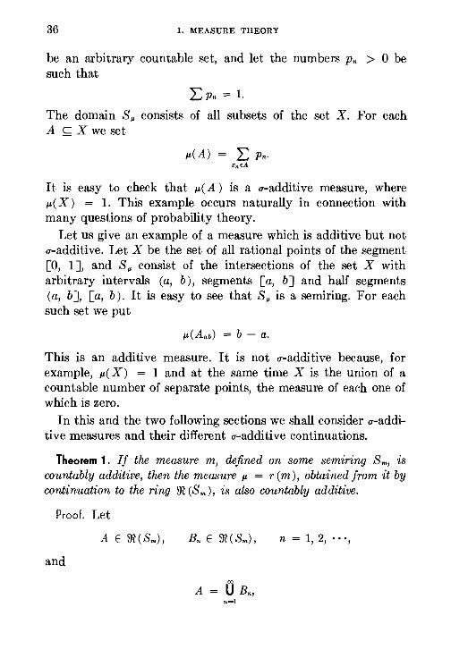
36 I. MEASURE THEORY
be an arbitrary countable set, and let the numbers Pn > 0 be such that
L Pn = 1.
The domain Sp. consists of all subsets of the set X. For each A s;;;; X we set
It is easy to check that ~(A ) is a u-additive measure, where ~(X) = 1. This example occurs naturally in connection with many questions of probability theory.
Let us give an example of a measure which is additive but not u-additive. Let X be the set of all rational points of the segment [0, 1 ], and S ~' consist of the intersections of the set X with arbitrary intervals (a, b), segments [a, b] and half segments (a, b ], [a, b). It is easy to see that S ~' is a semiring. For each such set we put
~(Aab) = b - a.
This is an additive measure. It is not u-additive because, for example, ~(X) = 1 and at the same time X is the union of a countable number of separate points, the measure of each one of which is zero.
In this and the two following sections we shall consider u-additive measures and their different u-additive continuations.
Theorem 1. If the measure m, defined on some semiring Sm, is countably additive, then the measure ~ = r ( m), obtained from it by continuation to the ring m (Sm), is also countably additive.
Proof. Let
n = 1, 2, · .. ,
and
n=l

5. COUNTABLE ADDITIVITY 37
where B, n Br Sm such that
5Zf for s ,e r. Then there exist sets A; and Bn; from
A = U A;,
where the sets on the right-hand sides of each of these equations are pairwise non-intersecting and the union over i and j is finite. (Theorem 3, §2).
Let Cnii = Bn; n A;. It is easy to see that the sets Cnii are pairwise non-intersecting, and hence,
A;= U U Cnii, n i
Therefore, and because of the additivity of the measure m on Sm, we have
m(A;) = L L m(Cn;;),
m(Bn;) = L m(Cnii),
and, by definition of the measure r( m) on m (Sm),
~(A) L m(A;),
(1)
(2)
(3)
(4)
Equations (1), (2), (3) and (4) imply ~(A) = L: ~(Bn). (The n
summations over i and j are finite, the series in n converge.) One could show that a Jordan continuation of a u-additive
measure is always u-additive; there is however no need to do this in this special case since it will follow from the theory of Lebesgue continuations which will be given in the next section.
Let us now show that, for the case of u-additive measures, Theorem 2 of §3 may be extended to countable coverings.
Theorem 2. If the measure ~ is u-additive, and the sets A, A1, A 2, • • ·, An, · · · belong to S ~'' then
n=l
38 J, MEASURE THEORY
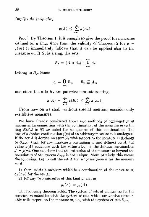
implies the inequality
~(A) ~ f: ~(An). n=l
Proof. By Theorem 1, it is enough to give the proof for measures defined on a ring, since from the validity of Theorem 2 for ~ = r( m) it immediately follows that it can be applied also to the measure m. If S ~' is a ring, the sets
n-1
Bn = (A nAn)"' U Ak k=l
belong to S p.· Since
n=l
and since the sets Bn are pairwise non-intersecting,
n=l n=l
From now on we shall, without special mention, consider only u-additive measures.
We have already considered above two methods of continuation of measures. In connection with the continuation of the measure m to the ring m(Sm) in §3 we noted the uniqueness of this continuation. The case of a Jordan continuationj(m) of an arbitrary measure m is analogous. If the set A is Jordan measurable with respect to the measure m (belongs to S;(m)), then, for any measure~ continuing m and defined on A, the value ~(A) coincides with the value J(A) of the Jordan continuation J = j(m). One can show that the extension of the measure m beyond the boundaries of the system S;(m) is not unique. More precisely this means the following. Let us call the set A the set of uniqueness for the measure m, if:
1) there exists a measure which is a continuation of the measure m, defined for the set A;
2) for any two measures of this kind ~~ and ~2
~,(A) = ~2(A).
The following theorem holds: The system of sets of uniqueness for the measure m coincides with the system of sets which are Jordan measurable with respect to the measure m, i.e., with the system of sets S;(m)·
6. LEBESGUE CONTINUATION OF MEASURE 39
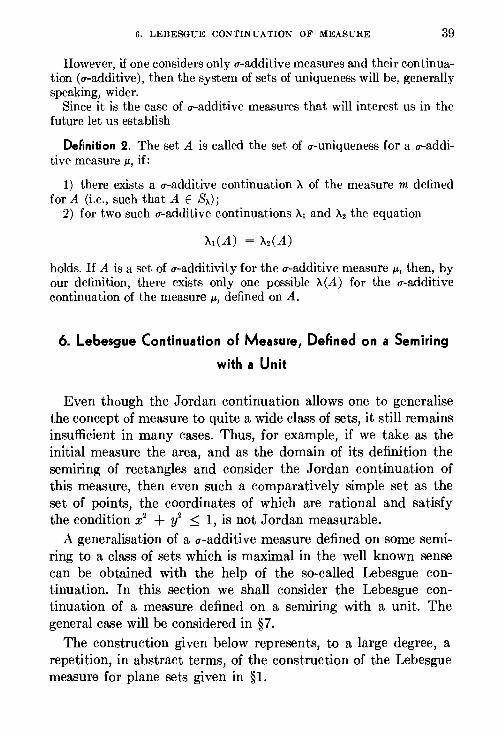
However, if one considers only u-additive measures and their continuation (u-additive), then the system of sets of uniqueness will be, generally speaking, wider.
Since it is the case of u-additive measures that will interest us in the future let us establish
DeAnition 2. The set A is called the set of u-uniqueness for a a--additive measure J.L, if:
1) there exists a u-additive continuation X of the measure m defined for A (i.e., such that A E Sx);
2) for two such u-additive continuations A1 and X2 the equation
holds. If A is a set of u-additivity for the u-additive measure J.L, then, by our definition, there exists only one possible X(A) for the u-additive continuation of the measure J.L, defined on A.
6. Lebesgue Continuation of Measure, DeAned on a Semiring
with a Unit
Even though the Jordan continuation allows one to generalise the concept of measure to quite a wide class of sets, it still remains insufficient in many cases. Thus, for example, if we take as the initial measure the area, and as the domain of its definition the seiniring of rectangles and consider the Jordan continuation of this measure, then even such a comparatively simple set as the set of points, the coordinates of which are rational and satisfy the condition x 2 + y2 s 1, is not Jordan measurable.
A generalisation of a a-additive measure defined on some seiniring to a class of sets which is maximal in the well known sense can be obtained with the help of the so-called Lebesgue continuation. In this section we shall consider the Lebesgue continuation of a measure defined on a seiniring with a unit. The general case will be considered in § 7.
The construction given below represents, to a large degree, a repetition, in abstract tenns, of the construction of the Lebesgue measure for plane sets given in §1.
40 I. MEASURE THEORY
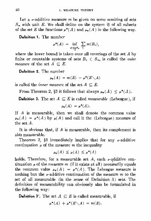
Let a u-additive measure m be given on some semiring of sets Sm with unit E. We shall define on the system ~ of all subsets of the set E the functions J.L *(A) and J.L* (A) in the following way.
Definition 1. The number
J.L*(A) = inf L m(Bn), A <:UBn n
n
where the lower bound is taken over all coverings of the set A by finite or countable systems of sets Bn E Sm, is called the outer measure of the set A s;;;; E.
Definition 2. The number
J.L*(A) = m(E) - J.L*(~A)
is called the inner measure of the set A ~ E.
From Theorem 2, §3 it follows that always J.L*(A) ::::;; J.L*(A).
Definition 3. The set A s;;;; E is called measurable (Lebesgue), if
~(A) = J.L*(A).
If A is measurable, then we shall denote the common value J.L*(A) = J.L*(A) by J.L(A) and call it the (Lebesgue) measure of the set A.
It is obvious that, if A is measurable, then its complement is alS'o measurable.
Theorem 2, §5 immediately implies that for any u-additive continuation J.L of the measure m the inequality
J.L*(A) ::::;; J.L(A) ::::;; J.L*(A)
holds. Therefore, for a measurable set A, each u-additive continuation J.L of the measure m (if it exists at all) nece~sarily equals the common value J.L* (A ) = J.L * (A). The Lebesgue measure is nothing but the u-additive continuation of the measure m to the set of all measurable (in the sense of Definition 3) sets. The definition of measurability can obviously also be formulated in the following way:
Definition 3'. The set A s;;;; E is called measurable, if
J.L*(A) + J.L*(E""'A) = m(E).
6. LEBESGUE CONTINUATION OF MEASURE 41
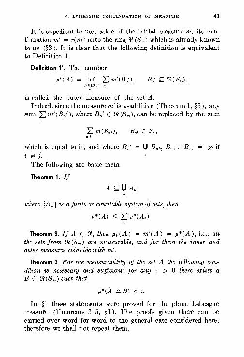
It is expedient to use, aside of the initial measure m, its continuation m' = r( m) onto the ring m (Sm) which is already known to us (§3 ). It is clear that the following definition is equivalent to Definition 1.
Definition 1 '. The number
~*(A) = inf L m' (En'), A£UBn' n
n
is called the outer measure of the set A. Indeed, since the measure m' is u-additive (Theorem 1, §5 ), any
sum L: m'(Bn'), where Bn' E m (Sm), can be replaced by the sum
n,k
which is equal to it, and where Bn' '/, ~ j.
The following are basic facts.
Theorem 1. If
A~ U An,
where {An) is a finite or countable system of sets, then
~*(A) s L ~*(An). "
.0 if
Theorem 2. If A E m, then ~*(A) = m'(A) = ~*(A), i.e., all the sets from m (Sm) are measurable, and for them the inner and outer measures coincide with m'.
Theorem 3. For the measurability of the set A the following condition is necessary and sufficient: for any z > 0 there exists a B E m (Sm) such that
~*(A D. B) < E.
In §1 these statements were proved for the plane Lebesgue measure (Theorems 3-5, §1 ). The proofs given there can be carried over word for word to the general case considered here, therefore we shall not repeat them.
42 I. MEASURE THEORY
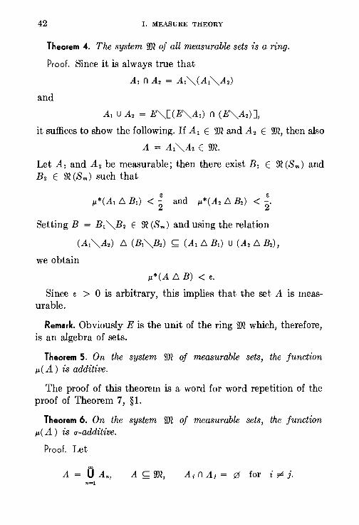
Theorem 4. The system 9R of all measurable sets is a ring.
Proof. Since it is always true that
A1 n A2 = A;"" (A1""A2)
and
A1 u A2 = E""[(~A1) n (~A2) ],
it suffices to show the following. If A1 E 9R and A2 E 9R, then also
A = A1""A2 E 9R.
Let A1 and A2 be measurable; then there exist B1 E m (Sm) and B2 E m (Sm) such that
e e ~*(A1 D. B1) < 2 and ~*(A2 D. B2) < 2"
Setting B = B1 ""B2 E m (Sm) and using the relation
(A1""A2) D. (B1""B2) s; (A1 D. B1) u (A2 D. B2),
we obtain
~*(A D. B) < e.
Since e > 0 is arbitrary, this implies that the set A is measurable.
Remark. Obviously E is the unit of the ring 9R which, therefore, is an algebra of sets.
Theorem 5. On the system 9R of measurable sets, the function ~c A) is additive.
The proof of this theorem is a word for word repetition of the proof of Theorem 7, §1.
Theorem 6. On the system 9R of measurable sets, the function ~(A ) is u-additive.
Proof. Let
A = U An, A s; 9R, A, n A; = 0 for i ~ j. n=l
6. LEBESGUE CONTINUATION OF MEASURE 43
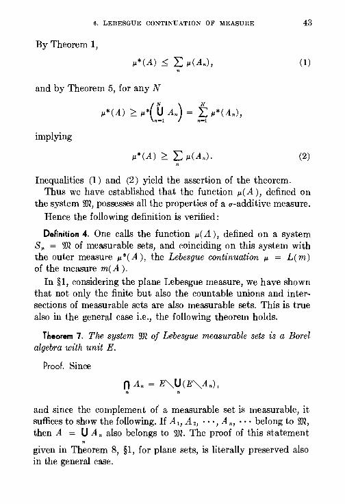
By Theorem 1,
(1)
and by Theorem 5, for any N
~*(A) ~ ~*C~l An) = !; ~*(An), implying
~*(A) ~ L ~(An). (2)
Inequalities (1) and (2) yield the assertion of the theorem. Thus we have established that the function ~(A), defined on
the system 9R, possesses all the properties of a u-additive measure. Hence the following definition is verified:
Definition 4. One calls the function ~(A ) , defined on a system Sp. = 9R of measurable sets, and coinciding on this system with the outer measure ~*(A ) , the Lebesgue continuation ~ = L( m) of the measure m( A ) .
In §1, considering the plane Lebesgue measure, we have shown that not only the finite but also the countable unions and intersections of measurable sets are also measurable sets. This is true also in the general case i.e., the following theorem holds.
Theorem 7. The system 9R of Lebesg·ue measurable sets is a Borel algebra with unit E.
Proof. Since
0 An = E"'U (E""An), n n
and since the complement of' a measurable set is measurable, it suffices to show the following. If A1, A 2, ···,An, · · · belong to 9R, then A = U An also belongs to 9)1. The proof of this statement
n
given in Theorem 8, §1, for plane sets, is literally preserved also in the general case.
44 I. MEASURE THEORY
Exactly as in the case of a plane Lebesgue measure its u-additivity implies its continuity, i.e., if J.L is a u-additive measure, defined on a B-algebra, A1 ::2 A 2 ::2 • • · ;;;;? An ::2 • • • is a decreasing chain of measurable sets and
then
and if A 1 s;;;; A 2 s;;;; measurable sets and
then
A = 0 An, n
J.L(A) = lim J.L(An),
s;;;; An c · · · is an increasing chain of
J.L(A) =lim J.L(An).
The proof given in §1 for a plane measure (Theorem 10) can be carried over to the general case.
1) From the results of §§5 and 6 it is easy to deduce that every set A which is Jordan measurable is Lebesgue measurable; moreover its Jordan and Lebesgue measures are equal. This immediately implies that the Jordan continuation of au-additive measure is u-additive.
2) Every set A which is Lebesgue measurable is a set of uniqueness for the initial measure m. Indeed, for any ~ > 0 there exists for A a B E m such that J.L*(A D. B) < ~. Whatever the extension X of the measure m may be,
X(B) = m' (B),
since the continuation Of the measure m to m = m(S.,) IS unique. Furthermore,
X(A D. B) s J.L*(A D. B) < e,
and therefore
IX(A) - m'(B) I <e. Thus we have, for two arbitrary continuations X1(A) and X2(A) of the measure m,
i. LEBESGUE CONTINUATION OF MEASURES 45
which, because of the arbitrariness of ~, implies
One can show that the system of Lebesgue measurable sets exhausts the whole system of sets of uniqueness for the initial measure m.
3) Let m be some u-additive measure with the domain of definition S and let 9R = L(S) be the domain of definition of its Lebesgue continuation. From Theorem 3 of this section it easily follows that whatever the semiring sl for which
we always have
L ( S1) = L ( S) .
7. Lebesgue Continuation of Measures
In the General Case
If the semiring Sm on which the initial measure m is defined does not have a unit, then the exposition of §6 must be slightly changed. Definition 1 of the outer measure is preserved, but the outer measure J.L* turns out to be defined only on the system S~'• of such sets A for which the coverings U Bn by sets from Sm with a finite sum n
L m(Bn)
exists. Definition 2 loses its meaning. The inner measure may be defined (in a slightly different way) also in the general case, but we shall not go into this. For the definition of measurability of sets it is expedient to take now the property of measurable sets implied by Theorem 3.
DeRnition 1. The set A is called measurable, if for any e > 0 there exists a set B E Sm such that J.L*(A D. B) < e.
Theorems 4, 5 and 6 and the final Definition 4 stay in force. In the proofs we used the assumption of the existence of a unit only in proving Theorem 4. To give the proof of Theorem 4 for the
46 I. MEASURE THEORY
general case we must show again that from A1 E M, A2 E M it follows that A1 u A2 E M. This proof is carried out exactly as for A 1 ""A 2 on the basis of the inclusion
In the case when Sm does not have a unit, Theorem 7, §6 IS
replaced by the following:
Theorem 1. For any initial measure m, the system of sets 9R =SL(m)
which are Lebesgue measurable is a a-ring. For measurable An the
set A = nQ1An is measurable if and only if the measures J.L CQ
1 An) are
bounded by some constant which does not depend on N.
The proof of this assertion is left to the reader.
Remark. In our exposition the measures are always finite, therefore the necessity of the last condition is obvious.
Theorem 1 implies the following
Corollary. The system 9RA of all sets B E 9R which are subsets of a fixed set A E 9R forms a Borel algebra.
For example, the system of all Lebesgue measurable (in the sense of the usual Lebesgue measure on the line) subsets of any segment [a, b] is a Borel algebra of sets.
In conclusion let us mention one more property of Lebesgue measures.
DeAnition 2. The measure J.L is called complete, if J.L(A) = 0 and A' ~A imply A' E Sp..
It is obvious that here J.L(A ') = 0. Without any difficulty one can show that the Lebesgue continuation of any measure is complete. This follows from the fact that for A' ~A and J.L(A) = 0 necessarily J.L*(A') = 0, and any set C for which J.L*(C) = 0 is measurable, since 0 E m and
J.L*(C D. 0) = J.L*(C) = 0.
7. LEBESGUE CONTINUATION OF MEASURES 47
Let us point out the connection between the process of Lebesgue continuation of measures and the process of completion of a metric space. For this let us note that m'(A D. B) can be taken as the distance between the elements A and B of the ring m(Sm). Then m(Sm) becomes a metric space (generally speaking not complete), a,nd its completion, by Theorem 3, §6, consists exactly of all the measurable sets. (Here, however, the sets A and B are indistinguishable, from the metric point of view, if ~(A D. B) = 0.)
CHAPTER II
MEASURABLE FUNCTIONS
8. Definition and Basic Properties of Measurable Functions
Let X and Y be two arbitrary sets, and assume that two systems of subsets 10 and 10', respectively, have been selected from them. The abstract function y = f(x), with the domain of definition X, taking on values from Y, is called (10, 10' )-measurable if from A E 10' it follows that j-1 (A) E 10.
For example, if we take as X and Y the real axis D 1 (i.e., consider real functions of a real variable), and as 10 and 10' take the system of all open (or all closed) subsets of Dt, then the stated definition of measurability reduces to the definition of continuity ( § 12 of Volume I). Taking for 10 and 10' the system of all Borel sets, we arrive at the so-called B-measurable (or Borel measurable) functions.
in what follows we shall be interested in the concept of measurability mainly from the point of view of the theory of integration. Of basic importance in this connection is the concept of ~-measurability of real functions, defined on some set X, where one takes for 10 the system of all ~-measurable subsets of the set X and for 10' the set of B-sets on the straight line. For simplicity, we shall assume that X is the unit of the domain of definition Sp. of the measure ~- Since, according to the results of §6, every u-additive measure can be continued to some Borel algebra, it is natural to assume from the beginning that S ~' is a B-algebra. Therefore we shall formulate the definition of measurability for real functions in the following way:
DeAnition 1 . The real function f( x), defined on the set X, IS
48
8. DEFINITION AND BASIC PROPERTIES 49
called ~-measurable if for any Borel set A of the real line
Let us denote the set of those x E X for which condition Q is satisfied by I x : Q ).
Theorem 1 . In order that the function f( x) be wmeasurable, it is necessary and sufficient that for any real C the set I x : f( x) < c) be !L-measurable (i.e., belongs to S~').
Proof. The necessity of the condition is clear, since the half line (- oo , c) is a Borel set. To prove the sufficiency let us first of all note that the Borel closure B (~) of the system ~ of all half lines (- oo , c) coincides with the system B 1 of all Borel sets of the real axis. By assumption, f- 1
( ~) s;;;; S p.· But then
and, since by assumption Sp. is a B-algebra, B(Sp.) theorem is thus proved.
Sp.. The
Theorem 2. The limit of a sequence of ~-measurable functions which converges for every x E X is ~-measurable.
Proof. Letfn(X)--> f(x), then
lx:f(x) < c} = u u n {x:fm(x) < c - k!}. (1) k n m>n
Indeed, if f( x) < c, then there exists a k, such that f( x) < c - 2jk; moreover, for this k one can find an n large enough so that for m ~ n the inequality
1 /m(x) < C - k
is satisfied, and this means that x will enter the right-hand side of (1 ).

50 II. MEASURABLE FUNCTIONS
Conversely, if x belongs to the right-hand side of (1 ), then there exists a k, such that, for all sufficiently large m,
butthenf(x) < c;i.e.,xenterstheleft-handsideofequation (1).
If the functions fn (x) are measurable, the sets
{x:fm(x) < c - H belong to Sp.. Since Sp. is a Borel algebra, the set
{x:f(x) < c)
also belongs to S ~'' by (1 ) , which proves that f( x) is measurable. For the further study of measurable functions it is convenient
to represent each of them as a limit of a sequence of so-called simple functions.
De~nition 2. The function f( x) is called simple if it is wmeasurable and takes on not more than a countable number of values.
It is clear that the concept of a simple function depends on the choice of the measure J.L·
The structure of simple functions is characterised by the following theorem :
Theorem 3. Thefunctionf(x), taking on not more than a countable number of values
is J.L-measurable if and only if all the sets
An = {x:f(x) = Yn}
are J.L-measurable.
Proof. The necessity of the condition is obvious, since every An is the inverse image of a set of one point { Yn), and every set of

8. DEFINITION AND BASIC PROPERTIES 51
one point is a Borel set. Sufficiency follows from the fact that by the conditions of the theorem the inverse image f- 1 (B) of any set B s;;;; D 1 is the union U An of not more than a countable
ynEB
number of measurable sets An, i.e., is measurable.
The further use of simple functions will be based on the following theorem.
Theorem 4. In order that the function f( x) be J.L-measurable it is necessary and sufficient that it be representable as a limit of a uniformly convergent sequence of simple functions.
Proof. The sufficiency is clear from Theorem 2. To show the necessity, let us consider an arbitrary measurable function f( x), and let us setfn(x) = mjn 1f mjn s f(x) < (m + 1)/n (herem are integers, and n are positive integers). It is clear that the functions fn(x) are simple; they converge uniformly to f(x) as n--> oo, since if(x) - fn(x) I s ljn.
Theorem 5. The sum of two wmeasurable functions ts J.L-measurable.
Proof. Let us first show this assertion for simple functions. If f( x) and g( x) are two simple functions taking on the values
and
respectively, then their sum h(x) = f(x) + g(x) can take on only the values h = f; + g;, where each of these values is taken on on the set
{x:h(x) = h} u ({x:f(x) = fd n {x:g(x) = g;}). (2) !;+o;=h
The number of possible values h is finite or countable and the corresponding sets {x : h(x) = h) are measurable, since the right-hand side of equation (2) is obviously a measurable set.

52 II. MEASURABLE FUNCTIONS
To prove the theorem for arbitrary measurable functions f( x)
and g(x), let us consider sequences of simple functions lfn(x)) and {gn(x)} which converge tof(x) and g(x), respectively. Then the simple functions f n ( x) + gn ( x) converge uniformly to the function f(x) + g(x), which, by Theorem 4, is measurable.
Theorem 6. A B-measurable function of a J.L-measurable function is J.L-measurable.
Proof. Let f( x) = cp[~( x) ], where <P is Borel measurable and ~ is J.L-measurable. If A s;;;; D 1 is an arbitrary J.L-measurable set, then its inverse image A' = cp- 1(A) is B-measurable, and the inverse image A" = ~- 1 (A') of the set A' is wmeasurable. Sincef-1(A) = A", the function f is measurable.
The theorem just proved is applicable, in particular, in the case of continuous functions <P (they are always B-measurable ).
Theorem 7. The product of J.L-measurable functions is wmeasurable.
Proof. Sincefg = t [(f + g) 2 - (f- g) 2], the assertion follows from Theorems 5 and 6, and the fact that cp(t) = t2 is a continuous function.
Exercise. Show that iff( x) is measurable and does not take on the value zero, then 1 If( x) is also measurable.
In studying measurable functions one can often neglect the values of a function on a set of measure zero. In connection with this let us introduce the following
Definition. Two functions f and g, defined on one and the same measurable set E, are called equivalent (denoted by f "' g), if
J.L{x:f(x) ~ g(x)) = 0.
One says that some property is satisfied almost everywhere onE, if it is satisfied at all points of E with the exception of points which form a set of measure zero. Thus we can say that two functions are equivalent if they coincide almost everywhere.
Theorem 8. If two functions f and g which are continuous on some segment E are equivalent, then they coincide.
8. DEFINITION AND BASIC PROPERTIES 53
Proof. Let us assume that, at some point Xo, f( Xo) ~ g( Xo), i.e., f( xo) - g( Xo) ~ 0. Since f - g is a continuous function, one can find a neighbourhood of the point xo, at all points of which the function f - g is different from zero. This neighbourhood has a positive measure; thus
,.L(x:f(x) ~ g(x)) > 0,
i.e., the continuous functions f and g cannot be equivalent if they take on different values at at least one point.
It is obvious that the equivalence of two arbitrary measurable functions (i.e., in general, discontinuous) does not at all imply their identity; for example, the function which is equal to unity at rational points and equal to zero at irrational points is equivalent to the function which is identically zero.
Theorem 9. The function f( x) which is defined on some measurable set E and is equivalent on this set to some measurable function g( x) is also measurable.
Indeed, from the definition of equivalence it follows that
{x:f(x) > a} and {x:g(x) > a}
can differ from each other only by a set of measure zero; hence if the second is measurable, so is the first.
The definition of a measurable function given above is quite formal. In 1913, N. N. Luzin proved the following theorem which shows that measurable functions are functions which, in a well known sense, can be approximated by continuous functions.
Luzin's Theorem. In order that the function f(x) be measurable on the segment [a, b] it is necessary and sufficient that for any ~ > 0 there exist a function cp(x) which is continuous on [a, b ], and such that
,.L(x:f(x) ~ cp(x)) S e.
In other words, a measurable function can be made continuous, if one excludes from consideration its values on a set of arbitrarily small measure. This property which Luzin called the C-property can be taken as a definition of a measurable function.
54 II. MEASURABLE FUNCTIONS
9. Sequences of Measurable Functions.
Dirferent Types of Convergence.
Theorems 5 and 7 of the preceding section show that arithmetic operations on measurable functions again lead to measurable functions. According to Theorem 2 of §8, the class of measurable functions, in contrast to the set of continuous functions, is also closed with respect to the operation of going to the limit. For measurable functions it is expedient to introduce, aside from the usual convergence at every point, several other definitions of convergence. These definitions of convergence, their basic properties and the connections between them will be investigated in the present section.
Definition 1. The sequence of functions fn(x), defined on some space with measure X, is said to converge almost everywhere to the function F(x), if
limfn(x) = F(x) (1)
for almost all x E X (i.e., the set of those points at which (1) does not hold has measure zero).
Example. The sequence of functions fn(x) = ( -x)n, defined on the segment [0, 1 ], converges as n--> oo to the function F( x) = 0 almost everywhere (precisely, everywhere with the exception of the point x = 1 ).
Theorem 2 of §8 admits of the following generalisation.
Theorem 1 . If the sequence of J.L-measurable functions f n ( x) converges to the function F(x) almost everywhere, then F(x) is also measurable.
Proof. Let A be that set on which
limfn(x) = F(x).
By the condition, J.L(E"'-A) = 0. The function F(x) is measurable on A by Theorem 2, §8. Since on a set of measure zero every function is obviously measurable, F( x) is measurable on E"'-A; therefore, it is also measurable on the set E.
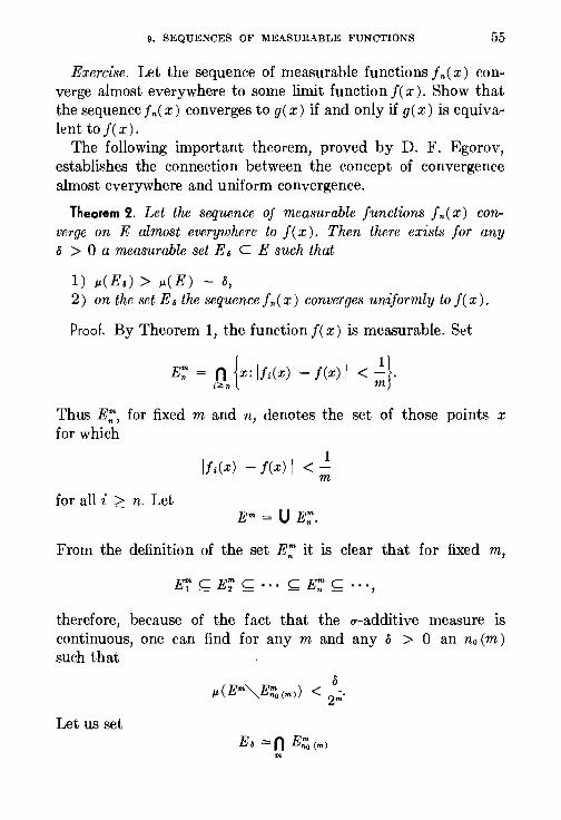
9. SEQUENCES OF MEASURABLE FUNCTIONS 55
Exercise. Let the sequence of measurable functions f n ( x) converge almost everywhere to some limit function f( x). Show that the sequence f n( x) converges to g( x) if and only if g( x) is equivalent to f(x).
The following important theorem, proved by D. F. Egorov, establishes the connection between the concept of convergence almost everywhere and uniform convergence.
Theorem 2. Let the sequence of measurable functions f n ( x) converge on E almost everywhere to f(x). Then there exists for any o > 0 a measurable set E a c E such that
1) J.L(Ea) > J.L(E) - o, 2) on the set Ea the sequencefn(x) converges uniformly to f(x).
Proof. By Theorem 1, the function f( x) is measurable. Set
E': = iOn {x: IJ;(x) - f(x) I < ~}·
Thus E;:, for fixed m and n, denotes the set of those points x for which
for all i ;::: n. Let
1 IJ;(x) - f(x) I < -
m
From the definition of the set E'; it is clear that for fixed m,
E'; ~ E'; ~ • • • ~ E';; ~ .. ·,
therefore, because of the fact that the u-additive measure is continuous, one can find for any m and any o > 0 an no (m) such that
Let us set Ea =n E::;,(m)
m
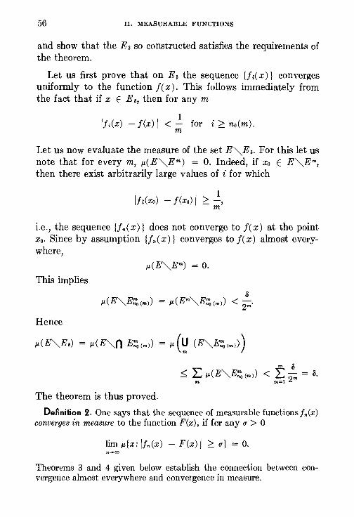
56 II. MEASURABLE FUNCTIONS
and show that the E 8 so constructed satisfies the requirements of the theorem.
Let us first prove that on E 8 the sequence {f;( x)) converges uniformly to the function f(x). This follows immediately from the fact that if x E Ea, then for any m
1 . lf;(x) - f(x) I < - for t ~ no(m).
m
Let us now evaluate the measure of the set E~E a. For this let us note that for every m, J.L(E~Em) = 0. Indeed, if x0 E E~Em, then there exist arbitrarily large values of i for which
1 IJ;(xo) - f(xo) I ~ -,
m
i.e., the sequence lfn(x)) does not converge to f(x) at the point xo. Since by assumption lfn(x)) converges to f(x) almost everywhere,
This implies
Hence
The theorem is thus proved.
De~nition 2. One says that the sequence of measurable functions fn(x) converges in measure to the function F(x), if for any u > 0
lim J.L{X: lfn(x) - F(x) I ~ u} = 0.
Theorems 3 and 4 given below establish the connection between convergence almost everywhere and convergence in measure.
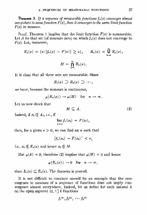
9. SEQUENCES OF MEASURABLE FUNCTIONS 57
Theorem 3. If a sequence of measurable functions fn(x) converges almost everywhere to some function F(x), then it converges to the same limit function F(x) in measure.
Proof. Theorem 1 implies that the limit function F(x) is measurable. Let A be that set (of measure zero) on which fn(x) does not converge to F(x). Let, moreover,
Rn(u)
ro
M = 0 Rn(u). n=l
It is clear that all these sets are measurable. Since
we have, because the measure is continuous,
J.L(Rn(u)) --> J.L(M) for n--> oo.
Let us now check that M~A. (2)
Indeed, if Xo EE A1, i.e., if
lim fn (xo) = F (xo),
then, for a given u > 0, we can find an n such that
lfn(Xo) - F(xo) I < u,,
i.e., Xo EE En(u) and hence Xo EE M.
But J.L(A) = 0, therefore (2) implies that J.L(M) = 0 and hence
J.L(Rn(u)) -->0 for n--> oo,
since En(u) s;;;; Rn(u). The theor~m is proved.
It is not difficult to convince oneself by an example that the convergence in measure of a sequence of functions does not imply convergence almost everywhere. Indeed, let us define for each natural k on the open segment (0, 1] k functions
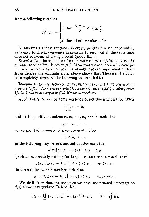
58 II. MEASURABLE FUNCTIONS
by the following method:
i i - 1 i
1 for -- < x <k - k'
[o for all other values of x.
Numbering all these functions in order, we obtain a sequence which, as is easy to check, converges in measure to zero, but at the same time does not converge at a single point (prove this!).
Exercise. Let the sequence of measurable functions fn(x) converge in measure to some limit functionf(x). Show that the sequence will converge in measure to the function g(x) if and only if g(x) is equivalent to f(x). Eve!l though the example given above shows that Theorem 3 cannot be completely reversed, the following theorem holds:
Theorem 4. Let the sequence of measurable functions fn(x) converge in measure to f(x). Then one can select from the sequence {fn(x)) a subsequence lfnk(x)) which converges to f(x) almost everywhere.
Proof. Let e1, e2, • • • be some sequence of positive numbers for which
lim en = 0,
and let the positive numbers 711, 712, • • ·, 1/n, • • • be such that
1/1 + 1/2 + ... converges. Let us construct a sequence of indices
n1 < n2 < · · · in the following way: n1 is a natural number such that
~{x: lfn,(x) - f(x) I ~ ed < 7]1
(such an n1 certainly exists); further, let n2 be a number such that
~{x: lfn,(x) - f(x) I ~ e2) < 1/2,
In general, let nk be a number such that
~{x: lfnk(x) - f(x) I ~ ek} < 1/k,
We shall show that the sequence we have constructed converges to f(x) almost everywhere. Indeed, let
R; = U {x: lfn&(x) - f(x) I ~ ek}, Q ro n R;.
k=i i=l
9. SEQUENCES OF MEASURABLE FUNCTIONS
Since R1 :J R2 :J Ra :J · · ·. :J Rn :J · · ·,
the continuity of the measure implies J.L(R;)--> J.L(Q).
59
On the other hand, it is clear that J.L(R;) < f: 7Jk, which yields J.L(R;) --> 0 fori--> oo. Since J.L(R;) --> 0, k=i
J.L(Q) = o. It remains to show that at all points of the set E~Q, the relation
fnk(x) --> f(x)
holds. Let Xo E E~Q. Then one can find an io such that Xo EE R;0 • This means that for all k ~ io
Xo EE {x:!fnk(x) -f(x)! ~ zk), i.e.,
Since, by assumption, Ek --> 0,
The theorem is proved.
CHAPTER Ill
THE LEBESGUE INTEGRAL
In the preceding chapter we investigated the basic properties of measurable functions, which are a quite wide generalisation of continuous functions. For measurable functions, the classical definition of an integral known from analysis and usually called the Riemann integral is generally not applicable. For example, the well known Dirichlet function which equals zero at irrational points is obviously measurable, but is not integrable in the sense of Riemann. Thus this concept of an integral turns out to be of little use with respect to measurable functions.
The reason for this is clear. Let us assume, for simplicity, that we are considering the functions on a segment. Introducing the concept of the Riemann integral, we split the segment on which the function f( x) is given into small segments, and taking in each of these parts an arbitrary point h, we form the sum
L:!Ch)dh k
Essentially, we replace here the value of the function f( x) at every point of the segment dXk = [xk, xk+!] by its value at some arbitrarily selected point ~k of this interval. However, it is only natural to do this if the values of the function f( x) at neighbouring points are close to each other, i.e., iff( x) is continuous or if the set of its points of discontinuity is "not too large".*
The basic idea of the Lebesgue integral consists of the fact that, as opposed to the Riemann integral, the points x are grouped not by their closeness on the x-axis, but by the closeness of the values of the functions at these points. This immediately gives rise to
• As is well known, a bounded function is integrable in the sense of Riemann if and only if the set of its points of discontinuity has measure zero.
60
10. LEBESGUE INTEGRAL FOR SIMPLE FUNCTIONS 61
the possibility of generalising the concept of the integral to a quite wide class of functions.
Moreover, the Lebesgue integral is defined in exactly the same way for functions which are defined in any spaces with measures, whereas the Riemann integral is first introduced for functions of one variable, and only then is it carried over with corresponding changes to the case of several variables.
Everywhere, where the contrary is not especially stated, we shall consider some u-additive measure ~(A) which is defined on a Borel algebra of sets with a unit X. All the sets A s;;;; X considered will be assumed to be u-measurable, and the functions f( x) to be defined for x E X and ~-measurable.
10. The Lebesgue lntegral·for Simple Functions
We shall first introduce the concept of a Lebesgue integral for functions which we called simple in the preceding section, i.e., for measurable functions which take on a finite or countable number of values.
Let f( x) be some simple function which takes on the values
Y1, Y2, • ··, Yn, • • ·, y; ~ Yi for t' ~ j.
It is natural to define the integral of the function f( x) over the set A by the equation
f f(x) d~ = L Yn~{x:x E A, f(x) = Yn}. (1) A n
Thus we arrive at the following definition.
De~nition. The simple function f( x) is called integrable (with respect to the measure ~) ove~ the set A if the sequence (1) converges absolutely. If f( x) is integrable, then the sum of the series (1) is called the integral off( x) over the set A.
In this definition we assume that all the Yn are different. One can, however, represent the value of the integral of a simple

62 III. LEBESGUE INTEGRAL
function as a sum of products of the form C•J.L( Bk) and not assume that all the ck are different. The following lemma allows us to do this:
Lemma. Let A = U Bk, B; n Bi = 0 for i ~ j, and assume that k
on each set B k the function f( x) takes on only one value c •. Then
(2)
moreover, the function f( x) is integrable over A if and only if the series (2) converges absolutely.
Proof. It is easy to see that every set
An = {x:x E A, f(x) = Yn}
is the union of those Bk for which ck = Yn· Therefore
L YnJ.L(An) = L Yn L J.L(Bk) L CkJ.L(Bk). ck=Yn k
Since the measure is non-negative,
L!Yn!J.L(An) = LlYn! L J.L(Bk) = L:!ck!J.L(Bk), n n ~~ k
i.e., the series L: YnJ.L (An) and L: CkJ.L (B.) both either converge n k
absolutely or diverge.
Let us establish some properties of the Lebesgue integral for simple functions:
A) i f(x) dJ.L + i g(x) dJ.L = i { f(x) + g(x)) dJ.L;
moreover, from the existence of the integrals on the left-hand side it follows that the integrals on the right-hand side exist.
To prove this let us assume that f( x) takes on the values f; on the sets F; c A, and g(x) the values g; on the sets G; s;;;; A, since
(3)
(4)
II, GENERAL DEFINITION AND BASIC PROPERTIES 63
Then, by the lemma,
J = JA { f(x) + g(x)) dJ.L = L: 'L:Cf; + Oi)J.L(F; n G;); (5) ' )
but J.L(F;) = L J.L(F; n G;),
i
J.L(G;) = L J.L(F; n G;).
Hence, from the absolute convergence of the series (3) and (4), there follows the absolute convergence of the series (5); here
J = Jl + J2.
B) For any constant k,
k i f(x) dJ.L = i {kf(x)) dJ.L;
moreover, the existence of the integral on the left-hand side implies the existence of the integral on the right. (This can be shown immediately.)
C) A simple function f( x) which is bounded on the set A is integrable over A; moreover, if if(x) I s MonA, then
(This can be shown immediately. )
11. General DeAnition and Basic Properties of the
Lebesgue Integral
Definition. We shall say that the function f( x) is integrable over the set A, if there exists a sequence of simple functions fn(X) which are integrable over A and converge uniformly to f( x). We shall denote the limit
(1)
64 III. LEBESGUE INTEGRAL
by i f(x) dp.
and call it the integral of the functionf(x) over the set A.
This definition is correct if the following conditions are satisfied:
1. The limit (1) for any uniformly convergent sequence of simple functions which are integrable over A exists.
2. This limit for a given functionf(x) does not depend on the choice of the sequence {fn(x) ).
3. For simple functions the definitions of integrability and integral are equivalent to those given in §10.
All these conditions are indeed satisfied. To prove the first it suffices to note that by properties A),
B) and C) for integrals of simple functions,
I
r
f fn(x) dp. - f fm(x) dp. S p.(A) sup lfn(x) - /m(x) 1. A A uA
To prove the second condition, we must consider the two sequences {fn(x)) and {fn*(x)), and use the fact that
S p.(A) {sup lfn(x) - f(x) I +sup lfn*(x) - f(x) I}· nA nA
Finally, to prove the third condition it suffices to consider the sequencefn(x) = f(x).
Let us establish the basic properties of the Lebesgue integral.
Theorem 1.
Proof. It follows immediately from the definition of the integral.
11. GENERAL DEFINITION AND BASIC PROPERTIES 65
Theorem 2. For any constant k,
k J f(x) dJ.L = J {kf(x)) dJ.L, A .1
where the existence of the integral on the left-hand side implies the existence of the integral on the right.
Proof. The proof is obtained from property B) by proceeding to the limit for an integral of simple functions.
Theorem 3.
~ f(x) dJ.L + ~ g(x) dJ.L = ~ { f(x) + g(x)) dJ.L,
where the existence of the integral on the left implies the existence of the integral on the right.
Proof. The proof is obtained from property A) by proceeding to the limit for an integral of simple functions.
Theorem 4. A function f( x) which is bounded on the set A is integrable over A.
Proof. The proof is obtained from property C) by proceeding to the limit for an integral of simple functions.
Theorem 5. Iff( x) ;:::_ 0, then
~f(x) dJ.L;::: 0
(assuming that the integral exists).
Proof. For simple functions this follows immediately from the definition; for the general case the proof is based on the possibility of approximating non-negative functions by non-negative simple functions (for example by the method, given in the proof of Theorem 4 of §9).
Corollary 1. Iff( x) ;::::_ g( x), then
~ f(x) dJ.L ;::::. ~ g(x) dJ.L.
66 III. LEBESGUE INTEGRAL
Corollary 2. If on A, m s f(x) s M, then
m~(A) s i f(x) d~ s M~(A).
Theorem 6. If
A = U An, A; n Al = 0 for i ~ j,
then
J f(x) d~ = L J f(x) d~; A n An
moreover, the existence of the integral on the left-hand side implies the existence of the integrals and the absolute convergence of the series on the right.
Proof. Let us first check the assertion of the theorem for a simple functionf(x), which takes on the values
Let
then
Bk = {x:x E A, f(x) = yk},
Bnk = {x:x E An, f(x) = yk};
Since, under the assumption of integrability of f(x) over A, the series L: yk~( Bk) converges absolutely, and the measure is non
k
negative, all the other series of the chain of equations (1 ) also converge absolutely.
In the case of an arbitrary function f( x), its integrability over A implies that for any e > 0 there exists a simple function g( x)
11. GENERAL DEFINITION AND BASIC PROPERTIES 67
which is integrable over A and satisfies the condition
lf(x) - g(x) I < z. (2)
For g(x),
J g(x) d/.1. = L: J g(x) dJ.L; A n An
(3)
moreover, g( x) is integrable over every set An and the series (3) converges absolutely. This last fact and the estimate (2) imply that f( x) is also integrable over every An, and
L f f(x) dJ.L - J g(x) dJ.L :::; L eJ.L(An) :::; eJ.L(A), n An An r1.
I ~ f(x) dJ.L - ~ g(x) dJ.L\ :::; eJ.L(A),
which together with (3) yields the absolute convergence of the
series L:/ f(x)dJ.L and the estimate n An
L J f(x) dJ.L - J f(x) dJ.L :::; 2e. n An A
Since e > 0 is arbitrary,
L J f(x) dJ.L = J f(x) dJ.L. n An A
Corollary. Iff( x) is integrable over A, then f( x) is also integrable over any A' s;;;; A.
Theorem 7. If the function cp( x) is integrable over A and I f( x) I :::; cp(x), thenf(x) is also integrfLble over A.
Proof. If f( x) and cp( x) are simple functions, then A can be represented as a union of a finite or countable number of sets, on each of which f( x) and cp( x) are constant:
f(x) = an,
68 III. LEBESGUE INTEGRAL
Since cp( x) is integrable, we have
L/ an/ ~(An) ~ L an~(An) = f cp(x) d~. n n A
Therefore f( x) is also integrable and
For the general case the theorem is proved by proceeding to the limit.
Theorem 8. The integrals
J1 = J f(x) d~, A
J2 = J /f(x) /d~ A
exist or do not exist simultaneously.
Proof. From the existence of the integral J 2 there follows the existence of the integral J1 by Theorem 7.
The converse follows, in the case of a simple function, from the definition of the integral, and in the general case it is proved by going to the limit and using the fact that always
/Ia I - I b/1 ~ I a - b /.
Theorem 9. (T chebichev Inequality) If cp( x) ~ 0 on A, then
~{x:x E A, cp(x) ~ c} s ! J cp(x) d~. C A
Proof. Setting
A' = {x:x E A, cp(x) ~ c),
we have
f cp(x) d~ = j cp(x) d~ + J cp(x) d~ ~ J cp(x) d~ ~ c~(A'). A AI A'-AI AI
12. LIMITING PROCESSES UNDER LEBESGUE INTEGRAL SIGN 69
Corollary. If ~ lf(x) Ia~ = 0,
then f( x) = 0 almost everywhere.
Indeed, by the Tchebichev inequality, we have
~{x:x E A, lf(x) I ~ ~} s n ~ lf(x) Ia~ = 0
for all n. Therefore
~{x:x E A, f(x) ~ 0) S f ~{x:x E A, lf(x) I ~ ~} = 0.
12. Limiting Processes Under the Lebesgue Integral Sign
The problem of proceeding to the limit under the integral sign, or, what is the same thing, of the possibility of term by term integration of a convergent series, is often encountered in various problems.
It was established in classical analysis that a sufficient condition for the possibility of such a limiting process is the uniform convergence of the corresponding series.
In this section we shall derive some theorems concerning limiting processes under the Lebesgue integral sign, which represent quite far reaching generalisations of the corresponding theorems of classical analysis.
Theorem 1. If the sequencefn(x) on A converges tof(x) and if for all n
lfn(_x) I S cp(x),
where cp( x) is integrable on A, then the limit function f( x) is integrable on A and
70 III. LEBESGUE INTEGRAL
Proof. From the conditions of the theorem it easily follows that [f(x) I ~ cp(x). Let
Ak = {x:k- 1 ~ cp(x) < k};
and also let
Bm = U Ak = {x:cp(x) ~ m}. k;:::m
By Theorem 6 of the preceding section
and the series ( *) converges absolutely.
Here
From the convergence of the series ( * ) there follows the existence of an m such that
. The inequality cp (x) < m holds on A ""Bm. By Egorov's theorem, A ""Bm can be represented in the form A ""Bm = C u D, where p.(D) < e/Sm and on the set C the sequence { fn} converges uniformly to f.
Let us select anN such that, for n > N, on the set C
[fn(x) - f(x) I < 5p.~C)' Then
12. LIMITING PROCESSES UNDER LEBESGUE INTEGRAL SIGN 71
Corollary. If lfn(X) I ~ M andfn(X) --'>f(x), then
i fn(x) dp.---'> i f(x) dp..
Remark. In as much as the values which the function takes on on the set of measure zero do not influence the value of the integral, it suffices to assume in Theorem 1 that {f n ( x) } converges to f( x) almost everywhere.
Theorem 2. Let, on the set A,
f1(x) ~ h(x) ~ • · · ~ fn(x) ~ · • ·,
where the functions fn(X) are integrable and their integrals are not greater than a certain constant :
i fn(X) dp. ~ K.
Then almost everywhere on A the limit
f(x) = limfn(x)
exists, the function f(x) is integrable on A, and
i fn(x) dp.---'> i f(x) dp..
(1)
On a set on which the limit (1 ) does not exist, the function f( x) can be given arbitrarily, for example assuming on this set f(x) = 0.
Proof. Let us assume f1C x) ~ 0, since the general case can be easily reduced to this by going over to the functions
fn(X) = fn(x) - !J(x) ·
Let us consider the set
n = {x:x E A,fn(x) ___, oo }.
It is easy to see that n = n u nn<rl, where r n
fln(r) = {x:x E A,fn(x) > r}.
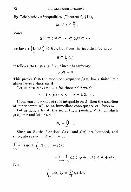
72 III. LEBESGUE INTEGRAL
By Tchebischev's inequalities (Theorem 9, §11 ), K
J.L(fln(r)) ~ - • T,
Since
we have J.L ( ~ n.<r>) ~ Kjr, but from the fact that for any r
it follows that J.L (n) ~ Kjr. Since r is arbitrary
J.L(n) = o.
This proves that the monotone sequence j.( x) has a finite liinit almost everywhere on A.
Let us now set cp( x) = r for those x for which
r - 1 ~ f(x) < r, T = 1, 2, • • •,
If one can show that cp(x) is integrable on A, then the assertion of our theorem will be an immediate consequence of Theorem 1.
Let us denote by Ar the set of those points x E A for which cp(x) = rand let us set
8
B. = U Ar. r=l
Since on· B. the functions j.(x) and f(x) are bounded, and since, always cp(x) ~ f(x) + 1,
J cp(x) dJ.L ~ J j(x) dJ.L + J.L(A) B 8 B 8
= ~~ i. j.(x) dJ.L + J.L(A) ~ K + J.L(A).
But
f cp(x) dJ.L = :t TJ.L(Ar). B 8 r=l
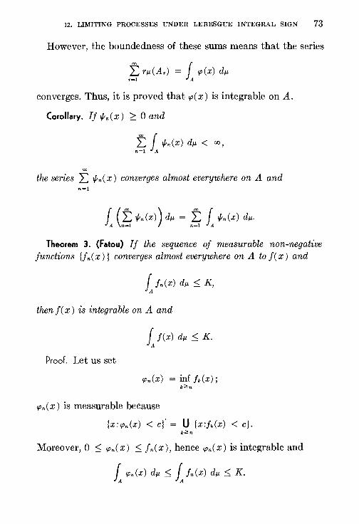
12. LIMITING PROCESSES UNDER LEBESGUE INTEGRAL SIGN 73
However, the boundedness of these sums means that the series
converges. Thus, it is proved that cp( x) is integrable on A.
Corollary. If if;n(X) ~ 0 and
f i if;,(x) dp. < oo,
ro
the series L if;n ( x) converges almost everywhere on A and n=l
Theorem 3. (Fatou) If the sequence of measurable non-negative functions lfn(x)} converges almost everywhere on A to f(x) and
then f( x) is integrable on A and
i f(x) dp. ~ K.
Proof. Let us set
<Pn(x) = inf fk(x); k:2:n
<Pn(X) is measurable because
{x:cpn(x) < c}' = U {x:fk(x) < c}. k;::.n
Moreover, 0 ~ <Pn(X) ~ fn(x), hence cpn(X) is integrable and
i cp.(x) dp. ~ i fn(x) dp. ~ K.
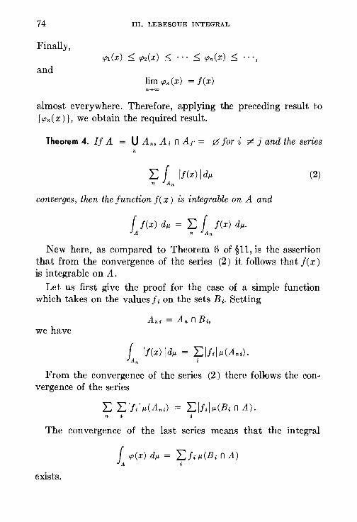
74 III. LEBESGUE INTEGRAL
Finally,
and lim 'Pn(x) = f(x)
almost everywhere. Therefore, applying the preceding result to {cpn(x) }, we obtain the required result.
Theorem 4. If A = U An, A; n Ar = [25 fori ~ j and the series
I: f IJCx) I all n An
(2)
converges, then the function f( x) is integrable on A and
New here, as compared to Theorem 6 of §11, is the assertion that from the convergence of the series (2) it follows that f(x) is integrable on A.
Let us first give the proof for the case of a simple function which takes on the values f; on the sets B;. Setting
An;= Ann B;, we have
From the convergence of the series (2) there follows the convergence of the series
L Ll!dll(An;) = L[J;[Jl(B; n A). n i i
The convergence of the last series means that the integral
exists.
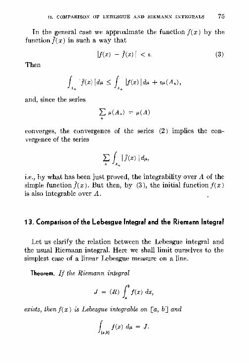
13. COMPARISON OF LEBESGUE AND RIEMANN INTEGRALS 75
In the general case we approximate the function f( x) by the function ](x) in such a way that
[J(x) - J(x) I < e. (3)
Then
and, since the series
converges, the convergence of the series (2) implies the convergence of the series
i.e., by what has been just proved, the integrability over A of the simple function]( x). But then, by (3 ), the initial function f( x)
is also integrable over A.
13. Comparison of the Lebesgue Integral and the Riemann Integral
Let us clarify the relation between the Lebesgue integral and the usual Riemann integral. Here we shall limit ourselves to the simplest case of a linear Lebesgue measure on a line.
Theorem. If the Riemann integral
J = (R) { f(x) dx, a
exists, thenj(x) is Lebesgue integrable on [a, b] and
J f(x) dJ.l. = J. [a,b]
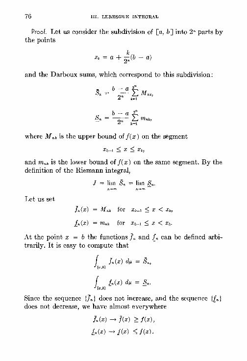
76 III. LEBESGUE INTEGRAL
Proof. Let us consider the subdivision of [a, b J into 2n parts by the points
k xk = a +
2Jb - a)
and the Darboux sums, which correspond to this subdivision:
where M nk is the upper bound off( x) on the segment
and mnk is the lower bound off( x) on the same segment. By the definition of the Riemann integral,
J = lim Sn = lim /in· n-+oo n-+oo
Let us set
At the point x = b the functions ]n and [n can be defined arbitrarily. It is easy to compute that
f ]n(X) dp. = Sn, [a,b]
f [n(X) dp. = /in• [a,b]
Since the sequence lln l does not increase, and the sequence {[n l does not decrease, we have almost everywhere
Jn(x) ~ J(x) ~ f(x),
i_n(x) ~ j(x) ~ f(x).
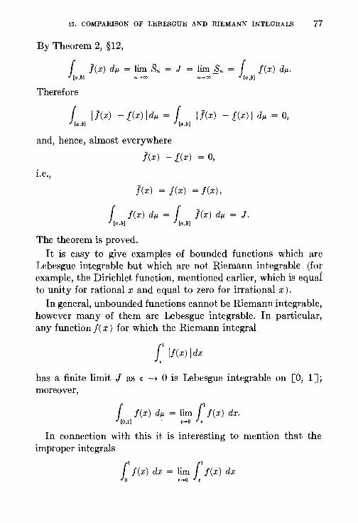
13. COMPARISON OF LEBESGUE AND RIEMANN INTEGRALS 77
By Theorem 2, §12,
f ](x) dJ.l. = lim Sn = J = lim §n = f [(x) dJJ.. [a,b] n-+oo n-+oo [a,b]
Therefore
f I ](x) - [(x) [dJJ. = J IJ(x) - .[(x)} dJ.l. = 0, ~~ ~~
and, hence, almost everywhere
](x) - [(x) = 0,
i.e.,
J(x) = j(x) = f(x),
J f(x) dJ.l. = J ](x) dJ.l. = J. [a,b] [a,b]
The theorem is proved. It is easy to give examples of bounded functions which are
Lebesgue integrable but which are not Riemann integrable (for example, the Dirichlet function, mentioned earlier, which is equal to unity for rational x and equal to zero for irrational x).
In general, unbounded functions cannot be Riemann integrable, however many of them are Lebesgue integrable. In particular, any function f( x) for which the Riemann integral
{ [f(x) [dx '
has a finite limit J as e ~ 0 is Lebesgue integrable on [0, 1]; moreover,
f f(x) dJ.l. = lim r f(x) dx. [0,1] • ,-+() '
In connection with this it is interesting to mention that the improper integrals
11
f(x) dx = lim r f(x) dx 0 £-<) f
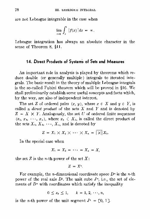
78 III. LEBESGUE INTEGRAL
are not Lebesgue integrable in the case when
lim { [f(x) [dx = oo. £-+0 f
Lebesgue integration has always an absolute character m the sense of Theorem 8, §11.
14. Direct Products of Systems of Sets and Measures
An important role in analysis is played by theorems which reduce double (or generally multiple) integrals to iterated integrals. The basic result in the theory of multiple Lebesgue integrals is the so-called Fubini theorem which will be proved in §16. We shall preliminarily establish some useful concepts and facts which, by the way, are also of independent interest.
The set Z of ordered pairs (x, y), where x E X and y E Y, is called a direct product of the sets X and Y and is denoted by Z = X X Y. Analogously, the set U of ordered finite sequences (x1, x2, · · ·, Xn), where xk E X k, is called the direct product of the sets X 1, X 2, • • ·, X n, and is denoted by
In the special case when
the set Z is the n-th power of the set X:
z = xn.
For example, then-dimensional coordinate space Dn is the n-th power of the real axis D 1• The unit cube Jn, i.e., the set of elements of Dn with coordinates which satisfy the inequality
k = 1, 2, · · ·, n,
is the n-th power of the unit segment J 1 = [0, 1].
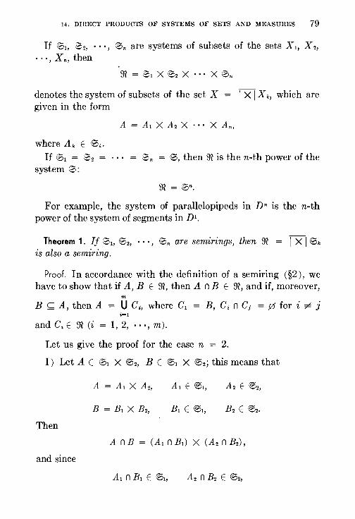
14. DIRECT PRODUCTS OF SYSTEMS OF SETS AND MEASURES 79
If 01, 0z, · · ·, 0n are systems of subsets of the sets X1, X z, · · ·, Xn, then
denotes the system of subsets of the set X = IX] X k, which are given in the form
where Ak E 10k.
If 01 = 0z system 0:
0n = 10, then ffi is the n-th power of the
For example, the system of parallelopipeds in Dn is the n-th power of the system of segments in D 1
•
Theorem 1. If 01, 0z, · · ·, 0n are semirings, then ffi is also a semiring.
Proof. In accordance with the definition of a semiring (§2), we have to show that if A, B E ffi, then A n B E ffi, and if, moreover,
m
B ~A, then A = U C;, where C1 = B, C; n C; = rz5 for i ~ j i=l
and C, E ffi (i = 1, 2, · · ·, m).
Let us give the proof for the case n = 2.
I) Let A E 01 X 10z, B E l01 X 10z; this means that
Then
and since
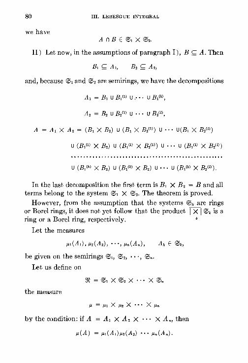
80 III. LEBESGUE INTEGRAL
we have A n B E l01 X l02.
II) Let now, in the assumptions of paragraph I), B ~ A. Then
and, because l01 and l02 are semirings, we have the decompositions
In the last decomposition the first term is B1 X B2 = Band all terms belong to the system l01 X l02. The theorem is proved. Howev~r, from the assumption that the systems 10k are rings
or Borel rings, it does not yet follow that the product fXI10k is a ring or a Borel ring, respectively. k
Let the measures
be given on the semirings l01, l02, · · ·, 10n. Let us define on
the measure
11- = 11-1 X 11-2 X · · · X P.n
by the condition: if A = A1 X A2 X · · · X An, then
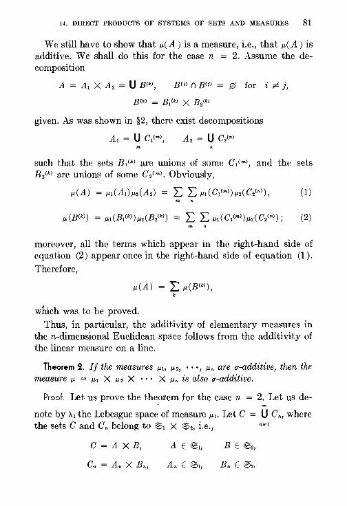
14. DIRECT PRODUCTS OF SYSTEMS OF SETS AND MEASURES 81
We still have to show that J.L(A) is a measure, i.e., that J.L(A) is additive. We shall do this for the case n = 2. Assume the decomposition
[25 for i ~ j,
given. As was shown in §2, there exist decompositions
such that the sets B1<k> are unions of some C1<m>, and the sets B2<k> are unions of some C2<m>. Obviously,
J.L(A) = J.Ll(AJ)J.L2(A2) = L L J.Ll(CJ(ml)J.L2(C2(nl), (1)
moreover, all the terms which appear in the right-hand side of equation (2) appear once in the right-hand side of equation (1 ).
Therefore,
which was to be proved. Thus, in particular, the additivity of elementary measures in
then-dimensional Euclidean space follows from the additivity of the linear measure on a line.
Theorem 2. If the measures J.Ll, J.L2, • • ·, J.Ln are u-additive, then the measure J.L = Ill X J.L2 X · · • X J.Ln is also u-additive.
Proof. Let us prove the theorem for the case n = 2. Let us de-• ro
note by A1 the Lebesgue space of measure Ill· Let C = U Cn, where the sets C and Cn belong to ~~ X ~2, i.e., n-=t
C =A X B,
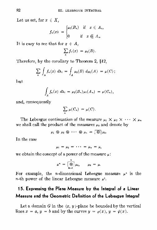
82 III. LEBESGUE INTEGRAL
Let us set, for x E X,
lJJ.2(Bn) if X E An, fn(x1 =
0 if X EE An.
It is easy to see that for x E A,
Lfn(X) =JJ.2(B).
Therefore, by the corollary to Theorem 2, §12,
L f fn(x) d\1 = f J.l.2(B) dJJ.!(A) = JJ.(C); n A A
but
and, consequently
The Lebesgue continuation of the measure /J.l X /J.2 X X J.l.n
we shall call the product of the measures /J.k and denote by
J.i.l ® J.1.2 ® · · • ® J.l.n = I ®I /J.k·
In the case
/J.l = /J.2 = ' ' ' = J.l.n = J.l.,
we obtain the concept of a power of the measure JJ.: n
J.l.n = I ®[JJ.k, /J.k = J.l.· k~l
For example, the n-dimensional Lebesgue measure J.l.n is the n-th power of the linear Lebesgue measure JJ. 1•
15. Expressing the Plane Measure by the Integral of a Linear
Measure and the Geometric Definition of the Lebesgue Integral
Let a domain G in the (x, y )-plane be bounded by the vertical lines x = a, y =band by the curves y = cp(x), y = if;(x).
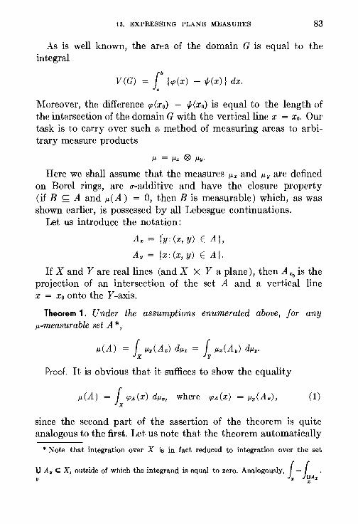
15. EXPRESSING PLANE MEASURES 83
As is well known, the area of the domain G is equal to the integral
V(G) = r {cp(x) - if;(x)} dx. a
Moreover, the difference cp(x0) - if;(xo) is equal to the length of the intersection of the domain G with the vertical line x = Xo. Our task is to carry over such a method of measuring areas to arbitrary measure products
Here we shall assume that the measures P.z and Jl.y are defined on Borel rings, are u-additive and have the closure property (if B ~ A and p.( A) = 0, then B is measurable) which, as was shown earlier, is possessed by all Lebesgue continuations.
Let us introduce the notation:
Ax = fy: (x, y) E A},
Ay = {x: (x, y) E A}.
If X and Yare real lines (and X X Y a plane), then Ax0
is the projection of an intersection of the set A and a vertical line x = Xo onto the Y -axis.
Theorem 1. Under the assumptions enumerated above, for any wmeasurable set A*,
p.(A) = L Jl.y(Ax) dp.x = ~ Jl.x(Ay) dp.y•
Proof. It is obvious that it suffices to show the equality
p.(A) = L <PA(x) dp.z, where 'PA(x) = p.y(Ax), (1)
since the second part of the assertion of the theorem is quite analogous to the first. Let us note that the theorem automatically
*Note that integration over X is in fact reduced to integration over the set
U A. c X, outside of which the integrand is equal to zero. Analogously, f = { . 'II 'II }~Ax
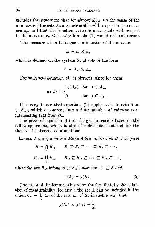
84 III. LEBESGUE INTEGRAL
includes the statement that for almost all x (in the sense of the Jl.x measure) the sets Ax are measurable with respect to the measure 11- y, and that the function cpA ( x) is measurable with respect to the measure 11-z· Otherwise formula (1 ) would not make sense.
The measure 11- is a Lebesgue continuation of the measure
which is defined on the system Sm pf sets of the form
For such sets equation (1 ) is obvious, since for them
It is easy to see that equation (1) applies also to sets from m (Sm), which decompose into a finite number of pairwise nonintersecting sets from Sm.
The proof of equation (1 ) for the general case is based on the following lemma, which is also of independent interest for the theory of Lebesgue continuations.
Lemma. For any p.-measurable set A there exists a set B of the form
Bnl ~ Bn2 ~ • • ' ~ Bnk ~ '' ',
where the sets Bnk belong to ffi (Sm); moreover, A ~ B and
p.(A) = p.(B). (2)
The proof of the lemma is based on the fact that, by the definition of measurability, for any n the set A can be included in the union C n = U dnr of the sets dnr of Sm in such a way that
1 p.(Cn) < p.(A) + -.
n
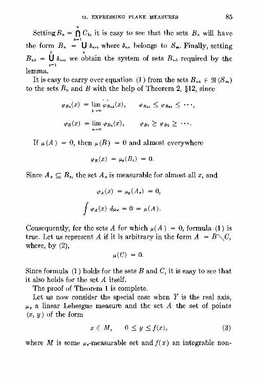
15. EXPRESSING PLANE MEASURES 85 n
SettingBn = n Ck, it is easy to see that the sets Bn will have k=l
the form Bn = U on., where on• belongs to Sm. Finally, setting k 8
Bnk = U on., we obtain the system of sets Bnk required by the s=l
lemma. It is easy to carry over equation (1 ) from the sets Bnk E ffi (S m)
to the sets Bn and B with the help of Theorem 2, §12, since
'PBn(x) = lim 'PBnk(x), 'P Bn! ~ 'P Bn2 ~ ' ' ' l k-ro
cp B1 ::::: cp B2 ::::: ' ' ' •
If 11- (A) = 0, then 11- (B) = 0 and almost everywhere
Since Ax ~ Bx, the set Ax is measurable for almost all x, and
<PA(x) = Jl.y(Ax) = 0,
J <PA(x) dp.x = 0 = p.(A).
Consequently, for the sets A for which p.( A) = 0, formula (1) is true. Let us represent A if it is arbitrary in the form A = B"" C, where, by (2),
p.(C) = 0.
Since formula (1) holds for the sets B and C, it is easy to see that it also holds for the set A itself.
The proof of Theorem 1 is complete. Let us now consider the special case when Y is the real axis,
Jl.y a linear Lebesgue measure and the set A the set of points (x, y) of the form
X EM, 0 ~ y ~f(x), (3)
where M is some 11-x-measurable set and f( x) an integrable non-
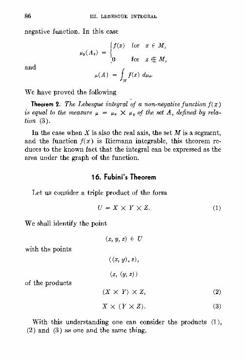
86 III. LEBESGUE INTEGRAL
negative function. In this case
and
jf(x) for x E M,
J.Ly(Ax) = O for x EE M,
J.L(A) = f f(x) dJ.Lx· .If
We have proved the following
Theorem 2. The Lebesgue integral of a non-negative function f( x) is equal to the measure J.L = J.Lx X J.Ly of the set A, defined by relation (3 ).
In the case when X is also the real axis, the set M is a segment, and the function f( x) is Riemann integrable, this theorem reduces to the known fact that the integral can be expressed as the area under the graph of the function.
16. Fubini's Theorem
Let us consider a triple product of the form
U =X X Y X Z.
We shall identify the point
with the points
of the products
(x, y, z) E U
((x,y),z),
(x, (y, z))
(X X Y) X Z,
X X (Y X Z).
(1)
(2)
(3)
With this understanding one can consider the products (1 ), (2 ) and (3 ) as one and the same thing.

16. FUBINI'S THEOREM 87
If the measures p.., 11-., Jl.z are given on X, Y, Z, then the measure
Jl.u = Jl.z @ Jl.y @ Jl.z
can be defined either as
or as Jl.u = Jl.x ® (p.y @ Jl.z) ·
The rigorous proof for the equivalence of these definitions is omitted here, although it is not difficult.
We shall give the application of these general constructions to the proof of the basic theorem of the theory of multiple integrals.
Fubini's Theorem. Let the measures Jl.x and Jl.y be defined on Borel rings, IT-additive and complete; let, moreover,
and let the function f( x, y) be integrable w1:th respect to the measure p. on the sets
Then*
J f(x, y) dp. = J (J f(x, y) dp..) dp.. = J (J f(x, y)dp..) dp. •. (4) A X A, Y Ay
Proof. The assertion of the theorem includes the existence of the inner integrals in parentheses for almost all values of the variable, with respect to which the integration in the parentheses is taken.
Let us first give the proof for the case f( x, y) > 0. For this purpose let us consider the triple product
U =X X Y X D\
where the third factor is the real axis, and the product of measures
where p.1 is a linear Lebesgue measure.
* See footnote on page 83.
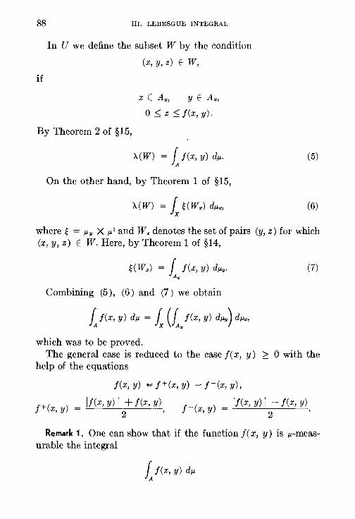
88
if
III. LEBESGUE INTEGRAL
In U we define the subset W by the condition
(x, y, z) E W,
0 ~ z ~ f(x, y).
By Theorem 2 of §15,
>-(W) = i f(x, y) dJJ..
On the other hand, by Theorem 1 of §15,
(5)
(6)
where~ = JJ. 11 X JJ. 1 and Wx denotes the set of pairs (y, z) for which (x, y, z) E W. Here, by Theorem 1 of §14,
(7)
Combining (5), (6) and (7) we obtain
which was to be proved. The general case is reduced to the case f(x, y) ;::: 0 with the
help of the equations
f(x,y) =j+(x,y) -j-(x,y),
! +( ) = lf(x, y) I + f(x, y) j-( ) = lf(x, y) I - f(x, y) x, y 2 ' x, y 2 .
Remark 1. One can show that if the function f( x, y) is JJ.-measurable the integral
i f(x, y) dJ.l.
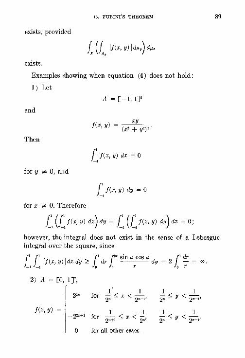
16. FUBINI'S THEOREM
exists, provided
exists.
Examples showing when equation (4) does not hold:
1) Let
A= [-1, 1]2
and
f(x, y) xy
Then
{ f(x, y) dx = 0 -1
for y ~ 0, and
r f(x, y) dy = 0 -1
for x ~ 0. Therefore
{1 (j_~ f(x, y) dx) dy = {
1 ({
1 f(x, y) dy) dx = 0;
89
however, the integral does not exist in the sense of a Lebesgue integral over the square, since
11 J1 [ 1 [211' sin cp cos cp [ 1 dr [f(x, y) [dx dy?: dr dcp = 2 - = oo. -1 -1 o o r o r
2) A = [0, lJ,
22n for ( 1
- <x <-2n - 2n-1' 1 1
- <y <-2n - 2n-1'
f(x, y) 1 1 1 1 -22n+1 for -<X<- -<y<-2n+l- 2n' 2n- 2n-1'
0 for all other cases.
90 III. LEBESGUE INTEGRAL
One can compute that
{ ({ f(x, y) dx) dy = 0, { ({ f(x, y) dy) dx = ~·
17. The Integral as a Set Function
Let us consider the integral F (A ) = J f( x )dx as a set function, ' A
assuming that S ~' is a Borel algebra with unit X and that
£f( x )dx exists. Then, as was shown earlier:
1. F(A) is defined on a Borel algebraS~'; 2. F( A) is real; 3. F( A) is additive, i.e., for every decomposition
A= U An
of the set A E S~' into the sets An E S~',
F(A) = L F(An);
4. F( A) IS absolutely continuous, i.e., J.L(A) F(A) = 0.
0 implies
Radon's Theorem. If the function F (A ) possesses the properties 1, 2, 3 and 4, then it may be represented in the form
F(A) = i j(x) dJ.L.
We shall show that the function f = dF /dJ.L can be uniquely determined up to values on a set of measure zero. Indeed, if for all A E S~',
17. THE INTEGRAL AS A SET FUNCTION 91
then for any n for the sets
An = {x:j2 - J1 > M we have
J.L(An) ~ n f Cf1 - !2) dJ.L = 0. An
Analogously, for
we have
J.L (Bn) = 0.
Since
Our assertion is proved.
CHAPTER IV
FUNCTIONS WHICH ARE SQUARE
INTEGRABLE
One of the most important spaces among the various linear normed spaces which are encountered in functional analysis is the Hilbert Space. Its name is due to the German mathematician D. Hilbert who introduced this space in connection with investigations in the theory of integral equations. It is a natural infinite analogue of the n-dimensional Euclidean space. We have already made acquaintance with one of the possible generalisations of Hilbert space in Chapter III of Volume I, it is the space Z2 whose elements are sequences of numbers
which satisfy the relation
n=l
The concept of the Lebesgue integral allows us to introduce another, in some cases more convenient, realisation of the same space-the space of square integrable functions. In this chapter we shall consider the definition and the basic properties of the space of square integrable functions and establish that it is isometric (with corresponding assumptions about the measure with respect to which the integration is performed) to the space z2.
In the next chapter we shall give an axiomatic definition of Hilbert space.
18. The L2 Space
Below we shall consider functions f( x), defined on some set R for which a measure JJ.(E) is given satisfying the condition
92
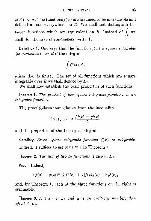
18. THE L2 SPACE 93
JJ.(R) < oo. The functionsf(x) are assumed to be measurable and defined almost everywhere on R. We shall not distinguish be-
tween functions which are equivalent on R. Instead of ~ we
shall, for the sake of conciseness, write J. Derinition 1. One says that the function f( x) is square integrable
(or summable) over R if the integral
exists (i.e., is finite). The set of all functions which are square integrable over R we shall denote by L2.
We shall now establish the basic properties of such functions.
Theorem 1. The product of two square integrable junctions is an integrable junction.
The proof follows immediately from the inequality
lf(x)g(x) I ~ f2(x) ~ g2(x)
and the properties of the Lebesgue integral.
Corollary. Every square integrable junction f( x) ts integrable.
Indeed, it suffices to set g( x) = 1 in Theorem 1.
Theorem 2. The sum of two L2 functions is also in L2.
Proof. Indeed,
(f(x) + g(x))2 ~ f 2 (x) + 2lf(x)g(x) I + g2(x),
and, by Theorem 1, each of the three functions on the right is summable.
Theorem 3. If f(x) E L 2 and a ts an arbitrary number, then af(x) E L2.
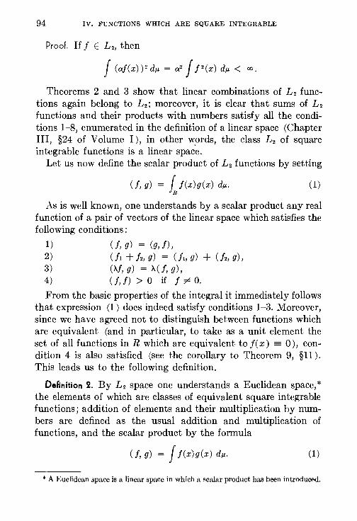
94 IV. FUNCTIONS WHICH ARE SQUARE INTEGRABLE
Proof. Iff E L2, then
J (af(x))2dp. = a 2 J j 2 (x) dp. < oo.
Theorems 2 and 3 show that linear combinations of L2 functions again belong to L2; moreover, it is clear that sums of L2 functions and their products with numbers satisfy all the conditions 1-8, enumerated in the definition of a linear space (Chapter III, §24 of Volume I), in other words, the class L2 of square integrable functions is a linear spac~.
Let us now define the scalar product of L2 functions by setting
(f, g) = i f(x)g(x) dp.. (1)
As is well known, one understands by a scalar product any real function of a pair of vectors of the linear space which satisfies the following conditions:
1) (f, g) = (g,f),
2) Ch +!2, g) = Ch g)+ Cf2, g), 3) (>..!,g) =>..(!,g), 4) ( j, f) > 0 if f -;;6- 0.
From the basic properties of the integral it immediately follows that expression (1) does indeed satisfy conditions 1-3. Moreover, since we have agreed not to distinguish between functions which are equivalent (and in particular, to take as a unit element the set of all functions in R which are equivalent to f( x) = 0), condition 4 is also satisfied (see the corollary to Theorem 9, §11 ). This leads us to the following definition.
DeAnition 2. By L2 space one understands a Euclidean space,* the elements of which are classes of equivalent square integrable functions; addition of elements and their multiplication by numbers are defined as the usual addition and multiplication of functions, and the scalar product by the formula
(!,g) = J f(x)g(x) dp.. (1)
* A Euclidean space is a linear space in which a scalar product has been introduced.
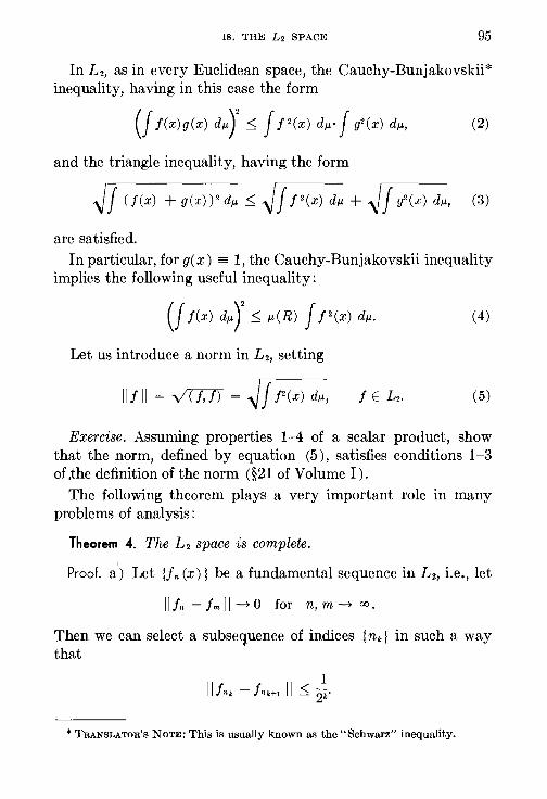
18. THE L2 SPACE 95
In L2, as in every Euclidean space, the Cauchy-Bunjakovskii* inequality, having in this case the form
(J f(x)g(x) dp.y ~ J f 2 (x) dw J g2(x) dp., (2)
and the triangle inequality, having the form
are satisfied. In particular, for g(x) = 1, the Cauchy-Bunjakovskii inequality
implies the following useful inequality:
(J f(x) dp. Y ~ p.(R) J f 2 (x) dp.. (4)
Let us introduce a norm in L2, setting
ll!ll = vrt:J) = ~~ f2(x) dp., (5)
Exercise. Assuming properties 1-4 of a scalar product, show that the norm, defined by equation (5), satisfies conditions 1-3 of,the definition of the norm (§21 of Volume 1).
The following theorem plays a very important role in many problems of analysis:
Theorem 4. The L 2 space is complete.
Proof. a') Let lfn (x)} be a fundamental sequence in L 2, i.e., let
llfn -fmii~O for n,m~ oo.
Then we can select a subsequence of indices { nk } in such a way that
*TRANSLATOR's NOTE: This is usually known as the "Schwarz" inequality.
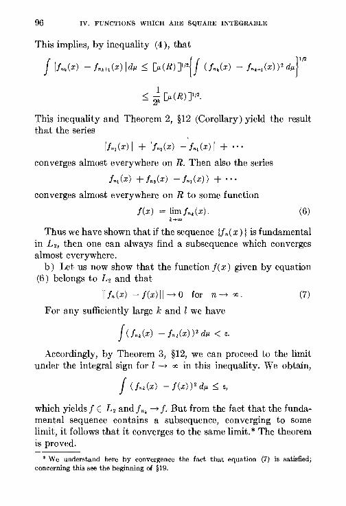
96 IV. FUNC'l'IONS WHICH ARE SQUARE INTEGRABLE
This implies, by inequality (4), that
J l!nk(x) - fnH1(x) [dll ~ [!l(R)]112{J Cfnk(x) - fnk+J(x)) 2 dllrf.!
~ ~ [ll ( R) ]112.
This inequality and Theorem 2, §12 (Corollary) yield the result that the series
converges almost everywhere on R. Then also the series
fn1 (x) + fn 2 (X) - fn1 (x)) + • • • converges almost everywhere on R to some function
f(x) = limfnk(x). (6)
Thus we have shown that if the sequence {fn( x)} is fundamental in L2, then one can always find a subsequence which converges almost everywhere.
b) Let us now show that the function f( x) given by equation (6) belongs to L2 and that
llfn(x) -f(x)JJ~o for n~ oo. (7)
For any sufficiently large k and l we have
f Cfnk(x) - fn 1(x) ) 2 d!l < e.
Accordingly, by Theorem 3, §12, we can proceed to the limit under the integral sign for l ~ oo in this inequality. We obtain,
J Cfnk(x) - f(x) )2 d!l ~ e,
which yields f E L2 and fnk ~f. But from the fact that the fundamental sequence contains a subsequence, converging to some limit, it follows that it converges to the same limit.* The theorem is proved.
* We understand here by convergence the fact that equation (7) is satisfied; concerning this see the beginning of §19.
!9. MEAN CONVERGENCE
19. Mean Convergence. Sets in L2 which are
Everywhere Complete.
97
Introducing a norm in L2 we have also introduced a certain kind of new convergence for the square integrable functions, namely:
(in~)
means that
lim J [j.(x) - f(x) ] 2 dJJ. = 0. n-ro
Such a convergence of functions is called convergence m the mean or, more exactly, convergence in the mean square.
Let us find the connection between the concept of convergence in the mean and uniform convergence, as well as the concept of convergence almost everywhere which we introduced in Chapter II.
Theorem 1. If the sequence lfn( x)} of functions in L2 converges uniformly tof(x), thenf(x) E L2 and {fn(x)} converges tof(x) in the mean.
Proof. Let e > 0. If n is sufficiently large, then
[fn(x) - f(x) I < e,
whence
This inequality immediately yields the assertion of the theorem. From Theorem 1 it follows that if one can approximate any
function f E L2 to an arbitrary degree of accuracy by functions fn E M ~ L2 in the sense of uniform convergence, then one can use them to approximate any function from L2 also in the sense of convergence in the mean.
Hence one can approximate any function f E L2 to any degree of accuracy by simple functions belonging to L2.
98 IV. FUNCTIONS WHICH ARE SQUARE INTEGRABLE
We shall show that any simple function f E L2, and therefore, also in general any function from L2, can be approximated as closely as desired by simple functions which take on only a finite number of values.
Let f( X) take on the values Yl, ••• ' y n, ... on the sets E l, En, · · ·. Since f2 is integrable, the series
L Yn2p.(En) = f J2(x) dp. n
converges. Let us select a number N in such a way that
and set for x E E;, i ~ N,
for x E E ;, i > N.
Then we have
i.e., the functions fN, which take on a finite number of values, approximate the function f as closely as required.
Let R be a metric space having a measure which satisfies the following condition (satisfied in all cases of practical interest) : all open and all closed sets in R are measurable and for any M ~R,
p.*(M) = inf p.(G), M_<;G
where the lower bound is taken over all open sets G containing M. Then the following theorem holds.
Theorem 2. The set of all continuous functions is complete in L2.
Proof. By what has been said above it suffices to show that every simple function which takes on a finite number of values is a limit, in the sense of mean convergence, of continuous functions. Furthermore, since every simple function which takes on a
19. MEAN CONVERGENCE 99
finite number of values is a linear combination of characteristic functions XM(x) of measurable sets, it suffices to give the proof for these latter ones. Let M be a measurable set in the metric space R. Then, from condition ( * ) it immediately follows that for any e > 0 one can find a closed set F M and an open set G M
for which
FM C M C GM and JJ.(G.lf) - JJ.(FM) < e.
Let us now define the function cp, ( x) by setting
k( ) _ p(x, R""G.~~) cp, x - p(x, R""GM) + p(x, F.lf)'
This function equals 0 for x E R""GM and equals 1 for x E FM. It is continuous since each of the functions p(x, F M) and p(x, R""GM) is continuous and since their sum is equal to zero. The function XM(x) - cp,(x) is not greater that unity on GM ""F and equals zero outside this set. Therefore
J (xM(x) - cp,(x) )2 dJJ. < e,
which yields the assertion of the theorem.
Theorem 3. If the sequence lfn( x)} converges to f( x) in the mean, then one can select from it a subsequence If nk( x) } which converges to f( x) almost everywhere.
Proof. If the sequence If n( x)} converges in the mean, then it is fundamental in L2; hence, repeating the arguments of part a) of the proof of Theorem 4, §18, we see that one can select from lfn( x)} a subsequence lfnk(x)} which converges almost everywhere to some function cp( x). Furthermore, the arguments of part b) of the same proof show that {fnk( x)} converges to cp( x) also in the mean, which yields cp( x) = f( x) almost everywhere.
It is not difficult to convince oneself by examples that the convergence in the mean of some sequence does not imply that this sequence itself converges almost everywhere. Indeed, the sequence of functions fnk constructed on page 57 obviously converges in the mean to the function f = 0 but still, as shown there, does not converge everywhere. We shall now show that convergence almost everywhere (and even everywhere)
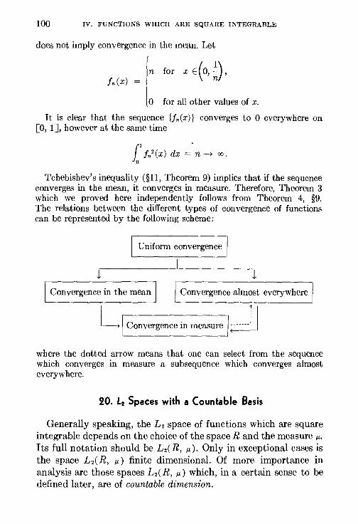
100 IV. FUNCTIONS WHICH ARE SQUARE INTEGRABLE
does not im:ply convergence in the mean. Let
1
( n for x E (o, ~) , fn(x) = n
0 for all other values of x.
It is clear that the sequence lfn(x)} converges to 0 everywhere on [0, 1], however at the same time
I ' f fn 2 (x) dx = n~ 00, 0
Tchebishev's inequality (§11, Theorem 9) implies that if the sequence converges in the mean, it converges in measure. Therefore, Theorem 3 which we proved here independently follows from Theorem 4, §9. The relations between the different types of convergence of functions can be represented by the following scheme:
Uniform convergence
I Convergence in the mean I Convergence almost everywhere
~~I Conve<gcnoc in mcaemc 1- ____ __; I
where the dotted arrow means that one can select from the sequence which converges in measure a subsequence which converges almost everywhere.
20. L2 Spaces with a Countable Basis
Generally speaking, the L2 space of functions which are square integrable depends on the choice of the spaceR and the measure p..
Its full notation should be L2( R, 11- ). Only in exceptional cases is the space L2( R, 11-) finite dimensional. Of more importance in analysis are those spaces L2( R, 11-) which, in a certain sense to be defined later, are of countable dimens1:on.
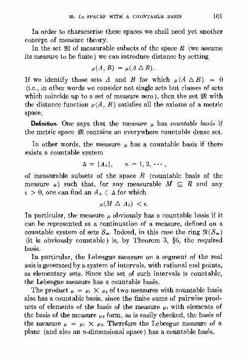
20. L2 SPACES WITH A COUNTABLE BASIS 101
In order to characterise these spaces we shall need yet another concept of measure theory.
In the set 9JC of measurable subsets of the spaceR (we assume its measure to be finite) we can introduce distance by setting
p(A, B) = J.L(A t::, B).
If we identify those sets A and B for which J.L (A 1:::, B) = 0 (i.e., in other words we consider not single sets but classes of sets which coincide up to a set of measure zero), then the set 9JC with the distance function p (A, B) satisfies all the axioms of a metric space.
De~nition. One says that the measure J.L has countable basis if the metric space 9JC contains an everywhere countable dense set.
In other words, the measure J.L has a countable basis if there exists a countable system
A= {An}, n = 1, 2, · · ·,
of measurable subsets of the space R (countable basis of the measure J.L) such that, for any measurable M ~ R and any E > 0, one can find an Ak E A for which
J.L(M 1:::, Ak) <E. In particular, the measure J.L obviously has a countable basis if it can be represented as a continuation of a measure, defined on a countable system of sets Sm. Indeed, in this case the ring fi(Sm)
(it is obviously countable) is, by Theorem 3, §6, the required basis.
In particular, the Lebesgue measure on a segment of the real axis is generated by a system of intervals, with rational end points, as elementary sets. Since the set of such intervals is countable, the Lebesgue measure has a countable basis.
The product J.L = Ill X J.L2 of two measures with countable basis also has a countable basis, since the finite sums of pairwise products of elements of the basis of the measure J.Ll with elements of the basis of the measure J.L2 form, as is easily checked, the basis of the measure J.L = Ill X J.L2· Therefore the Lebesgue measure of a plane (and also an n-dimensional space) has a countable basis.
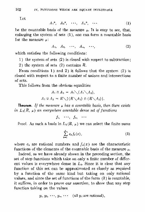
102 IV. FUNCTIONS WHICH ARE SQUARE INTEGRABLE
Let (1)
be the countable basis of the measure p.. It is easy to see, that, enlarging the system of sets (1 ) , one can form a countable basis for the measure 11-:
(2)
which satisfies the following conditions:
1 ) the system of sets (2) is closed with respect to subtraction; 2) the system of sets (2) contains R. From conditions 1 ) and 2) it follows that the system (2) is
closed with respect to a finite number of unions and intersections of sets.
This follows from the obvious equalities
A1 n A2 = A1""(A1""A2),
A1 u A2 = R""{ (R""A1) n (R""A2) }.
Theorem. If the measure 11- has a countable basis, then there exists in L 2C R, 11-) an everywhere countable dense set of functions
!J, •·•, fn,
Proof. As such a basis in L2 (R, 11-) we can select the finite sums
(3)
where ck are rational numbers and f k( x) are the characteristic functions of the elements of the countable basis of the measure p..
Indeed, as we have already shown in the preceding section, the set of step functions which take on only a finite number of different values is everywhere dense in L2. Since it is clear that any function of this set can be approximated as closely as required by a function of the same kind but taking on only rational values, and since the set of functions of the form (3) is countable, it suffices, in order to prove our assertion, to show that any step function taking on the values
y1, y2, · · ·, Yn, • • • (ally; are rational),

20. L2 SPACES WITH A COUNTABLE BASIS 103
on the sets
U E; = R, E; n Ei = [25 fori~j,
can be approximated as closely as desired in the sense of the L2
metric by a function of the form (3 ). By this remark, one can, without loss of generality, assume that our basis of the measure 11- satisfies conditions 1) and 2 ).
By the definition of a countable basis of the measure p., there exist, for any E > 0, sets A 1, A 2, ••• , An, . . • from our basis of measure p., such that p( E k, A k) < E, i.e.,
Let us set
and define
Ak' = Ak"" U A;, i<k
k = 1, 2, · · ·, n,
f*(x) 0 for x E R""U A/.
i=l
It is easy to see that for sufficiently small E the quantity
p.{x:j(x) ~ f*(x)}
is as small as required and, therefore, the integral
jCJ(x) -f*(x))2dp..::; (2max 1Ynl)2p.{x:f(x) ~f*(x)}
is arbitrarily small for sufficiently small E.
By virtue of our assumptlion concerning the basis of the measure p., the function f*( x) is a function of the form (3 ). The theorem is proved.
For the special case when R is a segment of the real line and p.
a Lebesgue measure, the countable basis in L2( R) can also be obtained by a more classical method: as such a basis we could
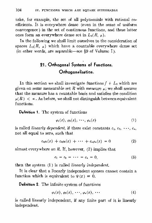
104 IV. FUNCTIONS WHICH ARE SQUARE INTEGRABLE
take, for example, the set of all polynomials with rational coefficients. It is everywhere dense (even in the sense of uniform convergence) in the set of continuous functions, and these latter ones form an everywhere dense set in L2(R, J.t).
In the following we shall limit ourselves to the consideration of spaces L2( R, J.t) which have a countable everywhere dense set (in other words, are separable----see §9 of Volume I).
21. Orthogonal Systems of Functions.
Orthogonalisation.
In this section we shall investigate functions f E L2 which are given on some measurable set R with measure J.t; we shall assume that the measure has a countable basis and satisfies the condition J.t( R) < oo. As before, we shall not distinguish between equivalent functions.
DeAnition 1. The system of functions
'Pi (X), 'P2 (X), " • , 'Pn (X) ( 1)
is called linearly dependent, if there exist constants ci, c2, • • ·, en, not all equal to zero, such that
Cicpi(x) + C2cp2(x) + • • • + Cncpn(x) = 0 (2)
almost everywhere on R. If, however, (2) implies that
Ci = C2 = • • • = Cn = 0, (3)
then the system (1 ) is called linearly independent.
It is clear that a linearly independent system cannot contain a function which is equivalent to 'lt (x) = 0.
DeAnition 2. The infinite system of functions
'Pi (X) , 'P2 (X) , " •, 'Pn (X), " • (4)
is called linearly independent, if any finite part of it is linearly independent.
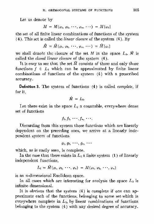
21, ORTHOGONAL SYSTEMS OF FUNCTIONS 105
Let us denote by
M = M ('PI, 'P2, ' ' ', <Pn, ' ' ') = M I cpk}
the set of all finite linear combinations of functions of the system ( 4). This set is called the linear closure of the system ( 4). By
M = M ('PI, <P2, " ', <Pn, • ") = M I cpk}
we shall denote the closure of the set M in the space L2. M is called the closed linear closure of the system (4 ).
It is easy to see that the set M consists of those and only those functions f E L2 which can be approximated by finite linear combinations of functions of the system (4) with a prescribed accuracy.
De~nition 3. The system of functions (4) is called complete, if for it,
!Jf = L2.
Let there exist in the space L2 a countable, everywhere dense set of functions
Discarding from this system those functions which are linearly dependent on the preceding ones, we arrive at a linearly independent system of functions
which, as is easily seen, is complete. In the case that there exists in L2 a finite system (1) of linearly
independent functions,
£2 = M(cpl, <P2, "·, <Pn) = M(cpl, <P2, "•, <Pn)
is an n-dimensional Euclidean space. In all cases which are interesting for analysis the space L2 is
infinite dimensional. It is obvious that the system (4) is complete if one can ap
proximate each of the functions, belonging to some set which is everywhere complete in L2, by linear combinations of functions belonging to the system ( 4 ) with any desired degree of accuracy.
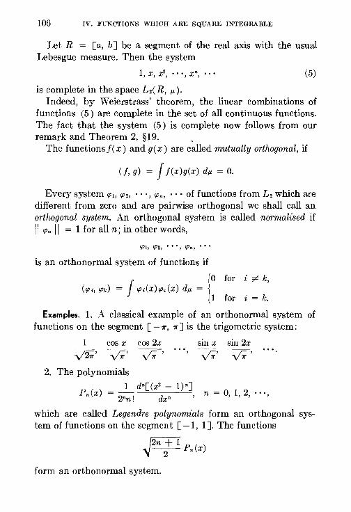
106 IV. FL"NCTIONS WHICH ARE SQUARE INTEGRABLE
Let R = [a, b] be a segment of the real axis with the usual Lebesgue measure. Then the system
(5)
is complete in the space L2( R, J.t). Indeed, by Weierstrass' theorem, the linear combinations of
functions (5) are complete in the set of all continuous functions. The fact that the system (5) is complete now follows from our remark and Theorem 2, §19. ,
The functions f( x) and g( x) are called mutually orthogonal, if
(f, g) = I f(x)g(x) d!J. = 0.
Every system cp1, cp2, • • ·, 'Pn, • • • of functions from L2 which are different from zero and are pairwise orthogonal we shall call an orthogonal system. An orthogonal system is called normalised if II 'Pn II = 1 for all n; in other words,
'PI, 'P21 ' ' ', 'Pn, ' ' '
is an orthonormal system of functions if
I (o for i -;;6- k,
(cpi, cpk) = cp;(x)cpk(x) d!J. = 11 l for i = k.
Examples. 1. A classical example of an orthonormal system of functions on the segment [ -1r, 1r] is the trigometric system:
1 cos x cos 2x sin x sin 2x
y27r' v;' y;' v;' v;' 2. The polynomials
1 dn[(x2 - 1)n] Pn(x) =
2-
1 d , nn. xn
n = 0, 1, 2, .. ·,
which are called Legendre polynomials form an orthogonal system of functions on the segment [ -1, 1]. The functions
~2n: 1 Pn(x)
form an orthonormal system.

21. ORTHOGONAL SYSTEMS OF FUNCTIONS 107
It is easy to see that an orthogonal system of functions is linearly independent. Indeed, multiplying the relation
Ci'Pl -'f- C2'P2 + ' ' ' + Cn'Pn = 0
by 'Pi and integrating, we obtain
ci(<Pi, cp;) = 0,
and since (cpi, cpi) > 0, we get ci = 0. Let us further note that, if in the space L2 there exists an every
where countable dense set f1, f2, · · ·, fn, · · •, then any orthonormal system of functions { 'Pa} is at most countable.
Indeed, let a ~ {3, then
II<Pa - <Pilll = 0. For each a let us select from our everywhere dense set an fa in such a way that
1 II<Pa -Jail< yl2"
It is clear that fa -;;6- ftl if a -;;6- {3, and, since the set of all the fa is countable, the set of the 'Pa themselves is also not more than countable.
In studying finite-dimensional spaces an important role is played by the concept of the orthogonal normalised basis, i.e., the orthogonal system of unit vectors, the linear closure of which coincides with the whole space. In the infinite case the analogue of such a basis is the complete orthonormal system of functions, i.e., a system
such that
1)
2)
(cpi, 'Pk) = oik,
M (cpi, 'P21'"' ', 'Pn, '• •) = £2.
Above we have given examples of complete orthonormal systems of functions on the segments [- 1r, 1r] and [ - 1, 1 ]. The existence of a complete orthonormal system of functions in any separable space L2 follows from the following theorem:
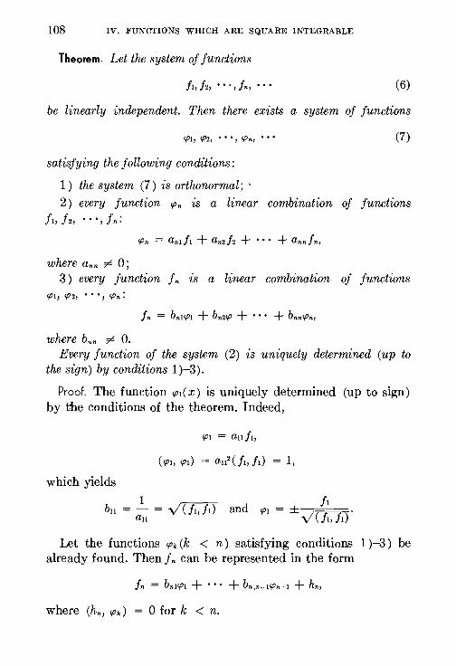
108 IV. FUNCTIONS WHICH ARE SQUARE INTEGRABLE
Theorem. Let the system of functions
(6)
be linearly independent. Then there exists a system of junctions
'PI, 'P2, • ' ', 'Pn, ' ' ' (7)
satisfying the following conditions:
1 ) the system (7 ) is orthonormal; · 2) every function 'Pn is a linear combination of functions
J1, J2, '' •, fn:
where ann -;;6- 0; 3 ) every junction f n is a linear combination of functions
'PI, 'P2, ' ' '' 'Pn:
where bnn -;;6- o. Every function of the system (2) is uniquely determined (up to
the sign) by conditions 1 )-3).
Proof. The function 'PI ( x) is uniquely detennined (up to sign) by the conditions of the theorem. Indeed,
which yields
1 bu =- = vC!J,!J)
au
Let the functions 'Pk (k < n) satisfying conditions 1 )-3) be already found. Then fn can be represented in the form
fn = bni'PI + ' '' + bn,n-I'Pn-1 + hn,
where (hn, 'Pk) = 0 for k < n.
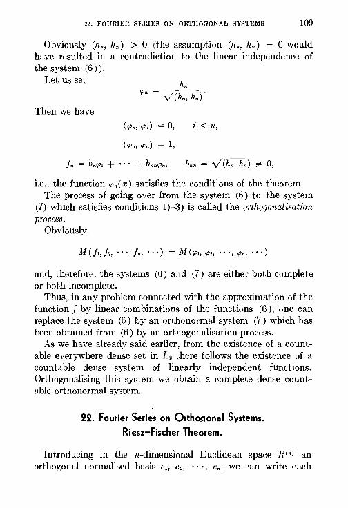
22. FOURIER SERIES ON ORTHOGONAL SYSTEMS 109
Obviously (hn, hn) > 0 (the assumption (hn, hn) = 0 would have resulted in a contradiction to the linear independence of the system (6 ) ) .
Let us set
Then we have
( 'Pn, cp;) = 0, i < n,
(cpn, 'Pn) = 1,
i.e., the function <Pn( x) satisfies the conditions of the theorem. The process of going over from the system (6) to the system
(7) which satisfies conditions 1 )-3) is called the orthogonalisation process.
Obviously,
and, therefore, the systems (6) and (7) are either both complete or both incomplete.
Thus, in any problem connected with the approximation of the function f by linear combinations of the functions (6 ), one can replace the system (6) by an orthonormal system (7) which has been obtained from (6) by an orthogonalisation process.
As we have already said earlier, from the existence of a countable everywhere dense set in L2 there follows the existence of a countable dense system of linearly independent functions. Orthogonalising this system we obtain a complete dense countable orthonormal system.
22. Fourier Series on Orthogonal Systems.
Riesz:-Fischer Theorem.
Introducing in the n-dimensional Euclidean space R<n> an orthogonal normalised basis e1, e2, • · ·, en, we can write each
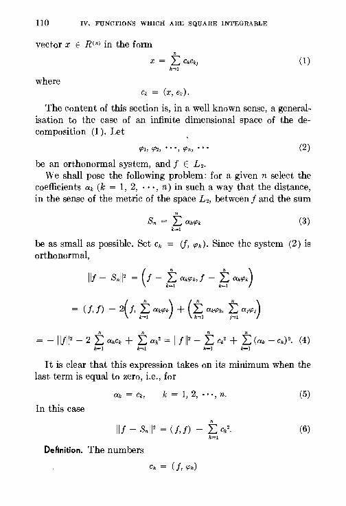
110 IV. FUNCTIONS WHICH ARE SQUARE INTEGRABLE
vector x E R<n> in the form
where
X = t Ckek1 k=i
Ck = (x, ek).
(1)
The content of this section is, in a well known sense, a generalisation to the case of an infinite dimensional space of the decomposition (1 ). Let
'PI, 'P2, ' ' ', 'Pn, ' ' ' (2)
be an orthonormal system, and f E L2. We shall pose the following problem: for a given n select the
coefficients ak ( k = 1, 2, · · · , n) in such a way that the distance, in the sense of the metric of the space L2, between f and the sum
(3)
be as small as possible. Set ck = (f, 'Pk). Since the system (2) is orthonormal,
IIJ- Snll2 = (J- J; CX.k'Pk, J- f CX.k'Pk)
= - IIJW- 2 t akck + t ak2 = 11!112- t Ck
2 + t (ak- ck) 2. (4) k=l k=l k=i k=l
It is clear that this expression takes on its minimum when the last term is equal to zero, i.e., for
k = 1, 2, .. ·, n. (5)
In this case
IIJ- SnW = (f,j) (6)
DeAnition. The numbers
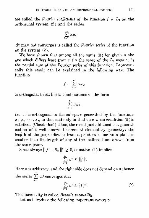
22. FOURIER SERIES ON ORTHOGONAL SYSTEMS 111
are called the Fourier coefficients of the function f E L2 on the orthogonal system (2 ) and the series
(it may not converge) is called the Fourier series of the function on the system (2 ) .
We have shown that among all the sums (3) for given n the one which differs least from f (in the sense of the L2 metric) is the partial sum of the Fourier series of this function. Geometrically this result can be explained in the following way. The function
n
! - I: Dlk'Pk k=l
is orthogonal to all linear combinations of the form
i.e., it is orthogonal to the subspace generated by the functions '/'1, <P2, • • ·, <Pn, in that and only in that case when condition (5) is satisfied. (Check this!) Thus, the result just obtained is a generalisation of a well known theorem of elementary geometry: the length of the perpendicular from a point to a line on a plane is smaller than the length of any of the inclined lines drawn from the same point.
Since always II!- Sn 11 2 ~ 0, equation (4) implies n
L Ck2 ~ 11!112
• k=i
Here n is arbitrary; and the right side does not depend on n; hence ro
the series I: ck2 converges and k=i
This inequality is called Bessel's inequality. Let us introduce the following important concept.
(7)

112 IV, FUNCTIONS WHICH ARE SQUARE INTEGRABLE
Definition. An orthonormal system (2) is called closed if for every function f E L2 the equation
(8)
holds, which one calls Parseval's equation.
One can see from ( 6) that the fact that the system (2) is closeci is equivalent to the fact tpat the partial sums of the Fourier series of each function f E L2 converge to fin the sense of the L 2 metric (i.e., in the mean).
The concept of closure of an orthonormal system is closely connected with the concept of completion of systems of functions introduced in §21.
Theorem 1. In L2 space every complete orthornomal system is closed, and conversely.
Proof. Let I <Pn( x)} be closed; then, whatever the function f E L2 may be, the sequence of partial sums of its Fourier series converges to it in the mean. This means that the linear combinations of elements of the system I<Pn(x)} are everywhere complete in L2, i.e., I 'Pn} is complete. Conversely, let I 'Pn} be complete, i.e., one can approximate any function f E L2 as closely as desired, in the sense of the L2 metric, by a linear combination
of elements I cpk} ; then the partial sum
n
L Ck'Pk k=l
of the Fourier series for f gives, generally speaking, an even closer approximation of the function f and, therefore, the series
converges to f in the mean, and Parseval's equality holds.
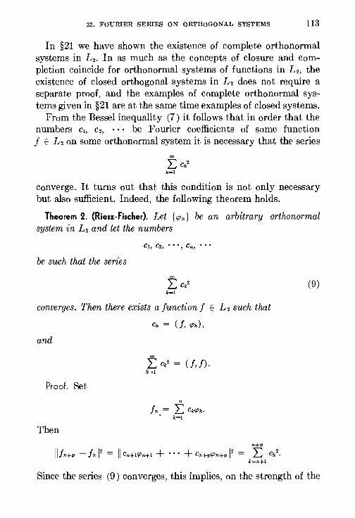
22. FOURIER SERIES ON ORTHOGONAL SYSTEMS 113
In §21 we have shown the existence of complete orthonormal systems in L2. In as much as the concepts of closure and completion coincide for orthonormal systems of functions in L2, the existence of closed orthogonal systems in L2 does not require a separate proof, and the examples of complete orthonormal systems given in §21 are at the same time examples of closed systems.
From the Bessel inequality (7) it follows that in order that the numbers c1, c2, • • • be Fourier coefficients of some function f E L2 on some orthonormal system it is necessary that the series
converge. It turns out that this condition is not only necessary but also sufficient. Indeed, the following theorem holds.
Theorem 2. (Riesz-fischer). Let { 'Pn} be an arbitrary orthonormal system in L2 and let the numbers
be such that the series
converges. Then there exists a function f E L 2 such that
Ck = (f, 'Pk),
and
f: Ck2 = (f, f). k~i
Proof. Set
Then n+p
llfn+p - fnll 2 = II Cn+i'Pn+l + ''' + Cn+p'Pn+pW = L Ck2
• k~n+l
(9)
Since the series (9) converges, this implies, on the strength of the
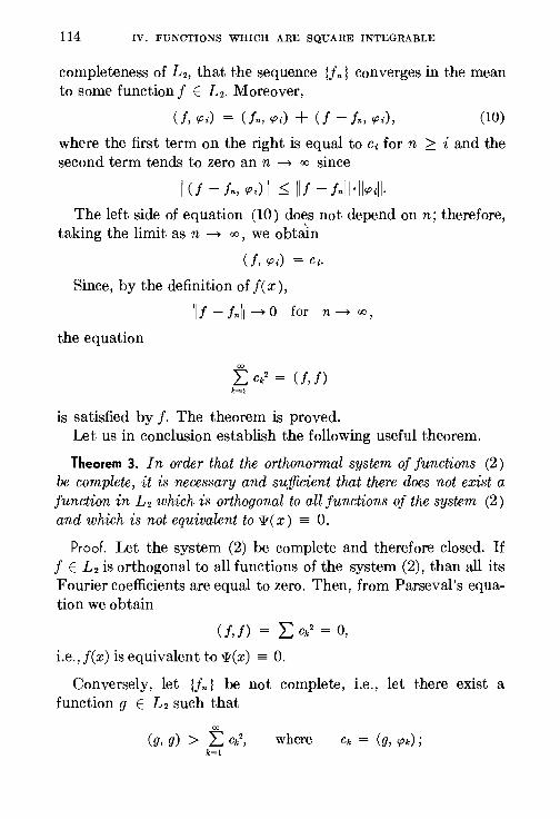
114 IV. FUNCTIONS WHICH ARE SQUARE INTEGRABLE
completeness of L2, that the sequence lfn} converges in the mean to some function f E L2. Moreover,
(f, cp;) = Cfn, 'Pi) + (f - fn, <Pi)' (10)
where the first term on the right is equal to c; for n ;::: i and the second term tends to zero an n ~ oo since
I CJ -in, <Pi) I ~ II! - !nll·II<Pill-The left side of equation (10) does not depend on n; therefore,
taking the limit as n ~ oo, we obtain
( j, cp;) = Ci•
Since, by the definition off( x),
II! -!nil ~ 0 for n ~ oo,
the equation
f: Ck2 = (f, f)
k=l
is satisfied by f. The theorem is proved. Let us in conclusion establish the following useful theorem.
Theorem 3. In order that the orthonormal system of functions (2) be complete, it is necessary and sufficient that there does not exist a junction in L2 which is orthogonal to all functions of the system (2) and which is not equivalent to 'lt( x) = 0.
Proof. Let the system (2) be complete and therefore closed. If f E L2 is orthogonal to all functions of the system (2), than all its Fourier coefficients are equal to zero. Then, from Parseval's equation we obtain
(f,f) = L Ck2 = 0,
i.e.,j(x) isequivalentto'lt(x) = 0.
Conversely, let lfn} be not complete, i.e., let there exist a function g E L2 such that
where
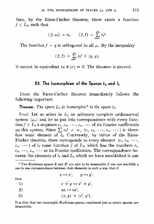
23. THE ISOMORPHISM OF SPACES L2 AND l2 115
then, by the Riesz-Fischer theorem, there exists a function f E L2, such that
( j, f) = f: ck2
• k-1
The function f - g is orthogonal to all cp;. By the inequality
(f, f) = f: ck2 < (g, g),
k-1
it cannot be equivalent to 'lt (x) = 0. The theorem is proved.
23. The Isomorphism of the Spaces L2 and 12
From the Riesz-Fischer theorem immediately follows the following important
Theorem. The space L2 is isomorphic* to the space l2.
Proof. Let us select in L2 an arbitrary complete orthonormal system { <Pn l and let us put into correspondence with every function f E L2 a sequence c1, c2, · • ·, Cn, • • • of its Fourier coefficients on this system. Since L Ck2 < oo, (c1, c2, • • ·, Cn, • • • ) is therefore some element of Z2. Conversely, by virtue of the RieszFischer theorem, there corresponds to every element (c1, c2, · · ·, Cn, ••• ) of z2 some function f of L2, which has the numbers c1, c2, · • ·, Cn, • • • as its Fourier coefficients. The correspondence between the elements of l2 and L2 which we have established is one
* Two Euclidean spaces R and R' are said to be isomorphic if one can establish a one to one correspondence between their elements in such a way that if
then
1)
2)
3)
x~x', y~y',
x +' y ~ x' + y',
ax~ ax',
(x, y) = (x', y').
It is clear that two isomorphic Euclidean spaces, considered just as metric spaces, are measurable.
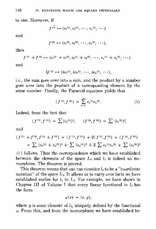
116 IV. FUNCTIONS WHICH ARE SQ"GARE INTEGRABLE
to one. Moreover, if
and
then
and
i.e., the sum goes over into a sum, and the product by a number goes over into the product of a corresponding element by the same number. Finally, the Parseval equation yields that
( J (I), J (2)) = f: Cn (i)Cn (2) •
Indeed, from the fact that
(JOJ,j(ll) = L(cn0l)2,
and
n=l
(f (2)' f (2))
(1)
(f (I) + j (2>, j (1) + j (2)) = (f (I)' j (1)) + 2 (f (I)' j (2)) + (f (2)' j (2))
= L (en(!) + Cn(2l)2 + L (cn°l)2 + 2 L Cn°lcn(2) + L (cn<2l)2
(1 ) follows. Thus the correspondence which we have established between the elements of the space L2 and Z2 is indeed an isomorphism. The theorem is proved.
This theorem means that one can consider Z2 to be a "coordinate notation" of the space L2. It allows us to carry over facts we have established earlier for Z2 to L2. For example, we have shown in Chapter III of Volume I that every linear functional in Z2 has the form
cp(x) = (x, y),
where y is some element of Z2, uniquely defined by the functional cp. From this, and from the isomorphism we have established be-
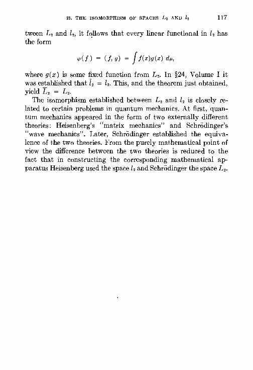
23. THE ISOMORPHISM OF SPACES L2 AND l2 117
tween L2 and Z2, it fqllows that every linear functional in Z2 has the form
cp(f) = (f, g) = J f(x)g(x) dJJ.,
where g(x) is some fixed function from L2. In §24, Volume I it was established that Z2 = l2. This, and the theorem just obtained, yield L2 = L2.
The isomorphism established between L2 and l2 is closely related to certain problems in quantum mechanics. At first, quantum mechanics appeared in the form of two externally different theories: Heisenberg's "matrix mechanics" and Schrodinger's "wave mechanics". Later, Schrodinger established the equivalence of the two theories. From the purely mathematical point of view the difference between the two theories is reduced to the fact that in constructing the corresponding mathematical apparatus Heisenberg used the space Z2 and Schrodinger the space L2.
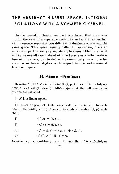
CHAPTER V
THE ABSTRACT HILBERT SPACE. INTEGRAL
EQUATIONS WITH A SYMMETRIC KERNEL.
In the preceding chapter we have established that the spaces L2 (in the case of a separable measure) and Z2 are isomorphic, i.e., in essence represent two different realisations of one and the same space. This space, usually called Hilbert space, plays an important part in analysis and its applications. Often it is useful not to tie oneself down ahead of time by one or another realisation of this space, but to define it axiomatically, as is done for example in linear algebra with respect to the n-dimensional Euclidean space.
24. Abstract Hilbert Space
De~nition 1. The set H of elements j, g, h, · · · of an arbitrary nature is called (abstract) Hilbert space, if the following conditipns are satisfied:
I. H is a linear space.
II. A scalar product of elements is defined in H, i.e., to each pair of elements f and g there corresponds a number (f, g) such that,
1)
2)
3)
4)
(f, g) = (g, f),
( aj, g) = a (f, g) ,
(h + h, g) = (fl, g) + (!2, g),
( j, f ) > 0 if f -;;6- 0.
In other words, conditions I and II mean that His a Euclidean 118

24. ABSTRACT HILBERT SPACE 119
space. The number II f II = v' (f, f) is called the norm of the element f.
III. The space H is complete in the sense of the p (f, g) = II f- g II metric.
IV. The space H is infinite-dimensional, i.e., for any natural n, one can find in H, n linearly independent vectors.
V. The space H is separable*, i.e., there exists in it a countable everywhere dense set.
It is easy to give examples of spaces which satisfy all the enumerated axioms. Such is the space Z2 which we considered in Chapter II of Volume I. Indeed, it is a Euclidean space, which is infinitely dimensional since, for example, its elements
e1 = ( 1, 0, 0, · • ·, 0, · · ·),
e2 = (0, 1, 0, · · ·, 0, • • ·),
e3 = (0, 0, 1, ... , 0, '"),
are linearly independent; the fact that it is complete and separable was proved in Chapter II, §9 and §13 of Volume I. The space L2 of functions which are square integrable with respect to some separable measure which is equivalent to Z2 also satisfies the same axioms.
The following statement holds: all Hilbert spaces are isomorphic. To prove this fact it obviously suffices to establish that every
Hilbert space is isomorphic to the coordinate space l2. This last assertion is proved in essence by the same considerations as the isomorphism of the spaces L2 and Z2, namely:
1) One can carry over to Hilbert space without any changes those definitions of orthogonality, closure and completeness which were introduced for the elements of the space L2 in §21.
2) Selecting in the Hilbert space H a countable everywhere dense set and applying to it 'the process of orthogonalisation described (for L2) in §21, we construct in H a complete orthonormal system of elements, i.e., the system
(1)
*Condition Vis often omitted, i.e., one considers nonseparable Hilbert spaces.
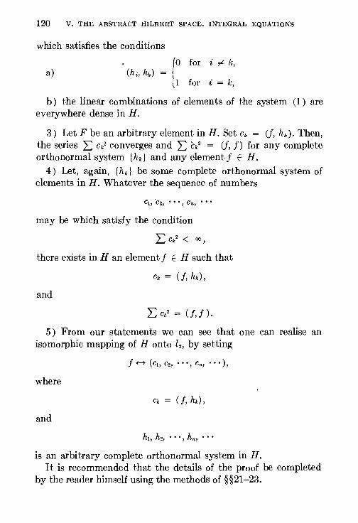
120 V. THE ABSTRACT HILBERT SPACE. INTEGRAL EQUATIONS
which satisfies the conditions
a) (o for i -;;6- k,
(hi, hk) = 11 l for i = k,
b) the linear combinations of elements of the system (1) are everywhere dense in H.
3) Let F be an arbitrary element in H. Set ck = (f, hk)· Then, the series I: ck2 converges and I: Ck2 = (f, f) for any complete orthonormal system {hd and any element f E H.
4) Let, again, { hk} be some complete orthonormal system of elements in H. Whatever the sequence of numbers
may be which satisfy the condition
there exists in H an element f E H such that
Ck = (f, hk),
and
5) From our statements we can see that one can realise an isomorphic mapping of H onto l2, by setting
where
and
is an arbitrary complete orthonormal system in H. It is recommended that the details of the proof be completed
by the reader himself using the methods of §§21-23.
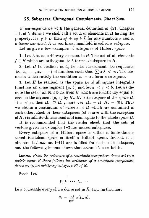
25. SUBSPACES. ORTHOGONAL COMPLEMENTS 121
25. Subspaces. Orthogonal Complements. Direct Sum.
In correspondence with the general definition of §21, Chapter III, of Volume I we shall call a set L of elements in H having the property: iff, g E L, then af + {3g E L for any numbers a and {3, a linear manifold. A closed linear manifold is called a subspace.
Let us give a few examples of subspaces of Hilbert space.
1. Let h be an arbitrary element in H. The set of all elements f E H which are orthogonal to h forms a subspace in H.
2. Let H be realised as l 2 , i.e., let its elements be sequences (xi, x2, · · ·, Xn, • • ·) of numbers such that L Xk 2 < oo. The elements which satisfy the condition xi = x2 form a subspace.
3. Let H be realised as the space L2 of all square integrable functions on some segment [a, b] and let a < c < b. Let us denote the set of all functions from H which are identically equal to zero on the segment [a, c] by He. He is a subspace of the space H. If Ci < c2, then He, ::J He,; moreover, Ha = H, Hb = (0). Thus we obtain a continuum of subsets of H which are contained in each other. Each of these subspaces (of course with the exception of Hb) is infinite-dimensional and isomorphic to the whole space H.
It is recommended that the reader check that the sets of vectors given in examples 1-3 are indeed subspaces.
Every subspace of a Hilbert space is either a finite-dimensional Euclidean space or itself a Hilbert space. Indeed, it is obvious that axioms I-III are fulfilled for each such subspace, and the following lemma shows that axiom IV also holds.
Lemma. From the existence of a countable everywhere dense set in a metric space R there follows the existence of a countable everywhere dense set in an arbitrary subspace R' of R.
Proof. Let
h, ~2, • • •, ~n, • • •
be a countable everywhere dense set in R. Let, furthermore,
an = inf p(~n, T/), ,•R'
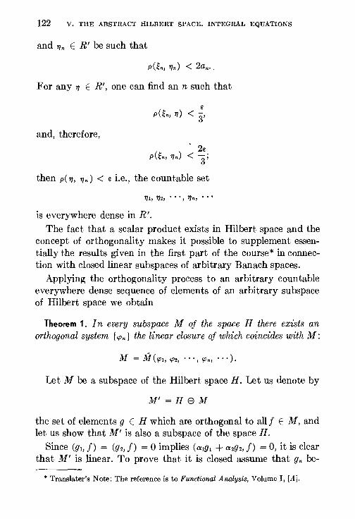
122 V. THE ABSTRACT HILBERT SPACE. INTEGRAL EQUATIONS
and T/n E R' be such that
For any 11 E R', one can find ann such that
and, therefore,
then p( 11, T/n) < E i.e., the countable set
T/1, T/2, ' ' ', T/n, ' ' '
is everywhere dense in R'. The fact that a scalar product exists in Hilbert space and the
concept of orthogonality makes it possible to supplement essentially the results given in the first part of the course* in connection with closed linear subspaces of arbitrary Banach spaces.
Applying the orthogonality process to an arbitrary countable everywhere dense sequence of elements of an arbitrary subspace of Hilbert space we obtain
Theorem 1. In every subspace M of the space H there exists an orthogonal system { <Pn } the linear closure of which coincides with M:
Let M be a subspace of the Hilbert space H. Let us denote by
M' = H 8 M
the set of elements g E H which are orthogonal to allf E M, and let us show that M' is also a subspace of the space H.
Since (g1, f) = (g2, f) = 0 implies (at[/! + a2g2, f) = 0, it is clear that M' is linear. To prove that it is closed assume that gn be-
* Translater's Note: The reference is to Functional Analysis, Volume I, [A].
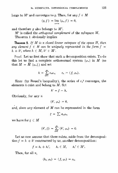
25. SUBSPACES. ORTHOGONAL COMPLEMENTS 123
longs toM' and converges to g. Then, for any f E M
(g, f) = lim (gn, f) = 0,
and therefore g also belongs to M'. M' is called the orthogonal complement of the subspace M. Theorem 1 obviously implies
Theorem 2. If M is a closed linear subspace of the space H, then any element f E H can be uniquely represented in the form f = h + h', where h E M, h' E M'.
Proof. Let us first show that such a decomposition exists. To do this let us find a complete orthonormal system { <Pn} in M (so that M = M {<Pn}) and set
h = f Cn'Pn, Cn = (f, <Pn) • n=l
Since (by Bessel's inequality), the series of Cn 2 converges, the elements h exist and belong toM. Set
h' = f- h.
Obviously, for any n
(h', <Pn) = 0, . and, since any element of M can be represented in the form
r = I: ancpn,
we have for t E M
(h', n = f (h', <Pn) = 0. n=l
Let us now assume that there exists, aside from the decomposition f = h + h' constructed· by us, another decomposition:
f =hi+ hi',
Then, for all n,
h/ EM'.
( J, <Pn) = Cn,
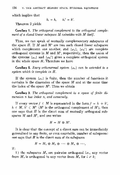
124 V. THE ABSTRACT HILBERT SPACE. INTEGRAL EQUATIONS
which implies that
Theorem 2 yields
Corollary 1. The orthogonal complement to the orthogonal complement of a closed linear subspace M coincides with M itself.
Thus, we can speak of mutually complementary subspaces of the space H. If M and M' are two such closed linear subspaces which complement one another, and {cpn}, {<Pm'} are complete orthogonal systems in M and M', respectively, then the union of the systems {cpn} and {cpm'} gives a complete orthogonal system in the whole space H. Therefore we have
Corollary 2. Every orthonormal system { 'Pn} can be extended to a system which is complete in H.
If the system {<Pn} is finite, then the number of functions it contains is the dimension of the space M and at the same time the index of the space M'. Thus we obtain
Corollary 3. The orthogonal complement to a space of finite dimension n has index n, and conversely.
If every vector f E M is represented in the form f = h + h', h E M, h' E M' (M' is the orthogonal complement of M), then one says that H is the direct sum of mutually orthogonal subspaces ]l,f and M', and one writes
H = M liB M'.
It is clear that the concept of a direct sum can be immediately generalised to any finite, or even countable, number of subspaces: one says that His the direct sum of its subspaces
H = M1 liB M2 liB • .. liB Mn liB .. ·,
if: 1) the subspaces M, are pairwise orthogonal i.e., any vector
from M. is orthogonal to any vector from Mk for i -;;6- k;
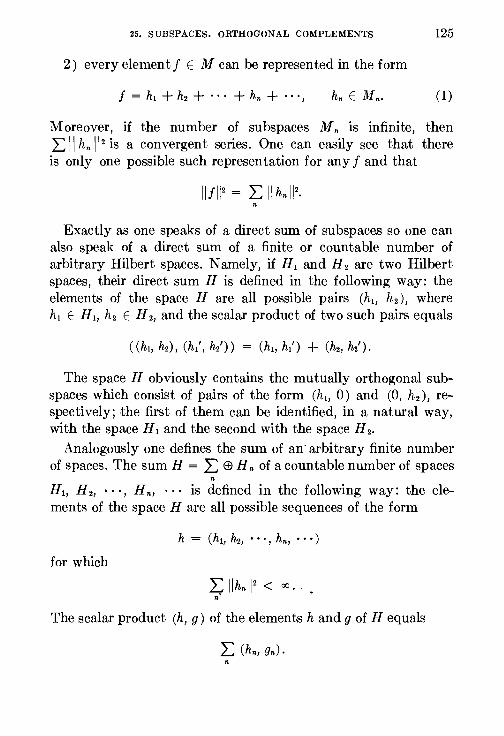
25, SUBSPACES. ORTHOGONAL COMPLEMENTS 125
2 ) every element f E M can be represented in the form
J = h1 + h2 + ' ' • + hn + • • •, (1)
Moreover, if the number of subspaces Mn is infinite, then I: II hn 11 2 is a convergent series. One can easily see that there is only one possible such representation for any f and that
11!112 = I: II hn 1!2• n
Exactly as one speaks of a direct sum of subspaces so one can also speak of a direct sum of a finite or countable number of arbitrary Hilbert spaces. Namely, if H1 and H 2 are two Hilbert spaces, their direct sum H is defined in the following way: the elements of the space H are all possible pairs (h1, h2), where h1 E H1, h2 E H 2, and the scalar product of two such pairs equals
The space H obviously contains the mutually orthogonal subspaces which consist of pairs of the form (h1, 0) and (0, h2 ), respectively; the first of them can be identified, in a natural way, with the space H1 and the second with the space H2.
Analogously one defines the sum of an· arbitrary finite number of spaces. The sum H = L liB H n of a countable number of spaces
n
H1, H 2, • • ·, H n, · · · is defined in the following way: the elementR of the space H are all possible sequences of the form
for which
The scalar product (h, g) of the elements h and g of H equals
n
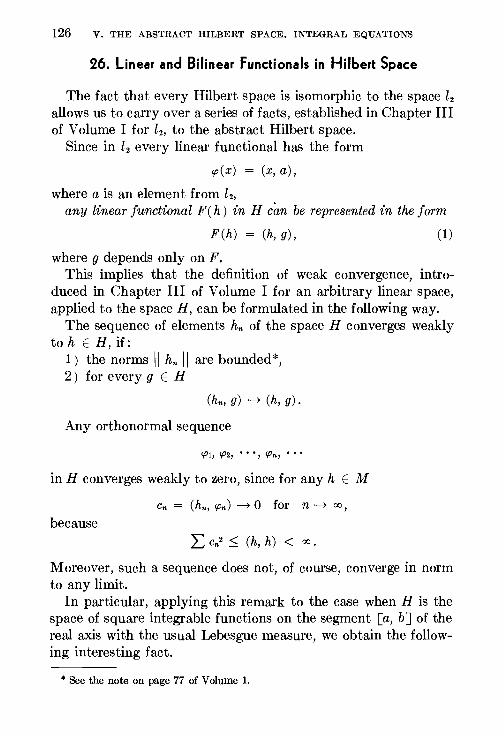
126 V. THE ABSTRACT HILBERT SPACE. INTEGRAL EQUATIONS
26. Linear and Bilinear Functionals in Hilbert Space
The fact that every Hilbert space is isomorphic to the space l2 allows us to carry over a series of facts, established in Chapter III of Volume I for l2, to the abstract Hilbert space.
Since in l2 every linear functional has the form
cp(x) = (x, a),
where a is an element from l2, any linear functional F (h) in H c(m be represented in the form
F(h) = (h,g), (1)
where g depends only on F. This implies that the definition of weak convergence, intro
duced in Chapter III of Volume I for an arbitrary linear space, applied to the space H, can be formulated in the following way.
The sequence of elements hn of the space H converges weakly to h E H, if:
1 ) the norms II hn II are bounded*, 2) for every g E H
(hn, g) ~ (h, g).
Any orthonormal sequence
'PI, 'P2 1 ' ' •, 'Pn, • • •
in H converges weakly to zero, since for any h E M
Cn = (hn, <Pn) ~ 0 for n ~ 00,
because L Cn2 .S (h, h) < 00.
Moreover, such a sequence does not, of course, converge in norm to any limit.
In particular, applying this remark to the case when H is the space of square integrable functions on the segment [a, b] of the real axis with the usual Lebesgue measure, we obtain the following interesting fact.
* See the note on page 77 of Volume 1.
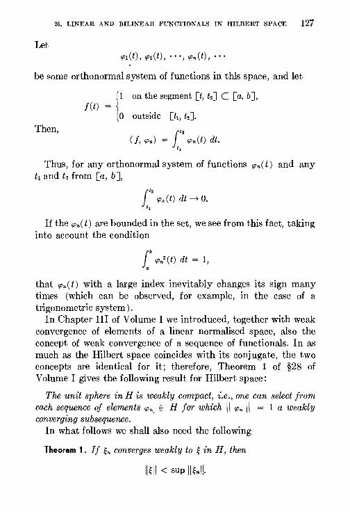
26. LINEAR AND BILINEAR FUNCTIONALS IN IULBERT SPACE 127
Let 'Pl(t), cp2(t), ... , <Pn(t), •••
be some orthonormal system of functions in this space, and let
Then, 1
1 on the segment [t, t2J C [a, b ], j(t) = 0
outside [t1, t2].
ft,
(f, <Pn) = 'Pn (t) dt. t,
Thus, for any orthonormal system of functions cpn( t) and any t1 and t2 from [a, b ],
ft,
cp.(t) at~o. t,
If the cpn(t) are bounded in the set, we see from this fact, taking into account the condition
t 'Pn2 (t) dt = 1, a
that <Pn(t) with a large index inevitably changes its sign many times (which can be observed, for example, in the case of a trigonometric system).
In Chapter III of Volume I we introduced, together with weak convergence of elements of a linear normalised space, also the concept of weak convergence of a sequence of functionals. In as much as the Hilbert space coincides with its conjugate, the two concepts are identical for it; therefore, Theorem 1 of §28 of Volume I gives the following result for Hilbert space:
The unit sphere in His weakly compact, i.e., one can select from each sequence of elements 'Pn, E H for which II 'Pn II = 1 a weakly converging subsequence.
In what follows we shall also need the following
Theorem 1. If ~n converges weakly to ~in H, then
11~11 < sup ll~nll.
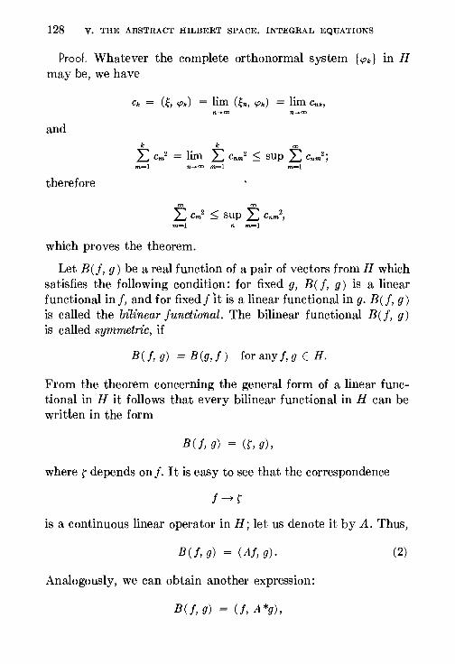
128 V. THE ABSTRACT HILBERT SPACE. INTEGRAL EQUATIONS
Proof. Whatever the complete orthonormal system { 'Pk} in H may be, we have
and k k ro
L Cm2 = lim L Cnm
2 ~ sup L Cnm2
; m=l n-+oo m=l m=l
therefore
t Cm2 ~ SUp t Cnm
21
m=l n m=l
which proves the theorem.
Let B(f, g) be a real function of a pair of vectors from H which satisfies the following condition: for fixed g, B(f, g) is a linear functional in f, and for fixed fit is a linear functional in g. B(f, g)
is called the bilinear functional. The bilinear functional B(f, g) is called symmetric, if
B(f, g) = B(g, f) for any j, g E H.
From the theorem concerning the general form of a linear functional in H it follows that every bilinear functional in H can be written in the form
BCJ, g) = cr, g),
where r depends on f. It is easy to see that the correspondence
is a continuous linear operator in H; let us denote it by A. Thus,
B(f, g) = (Aj, g). (2)
Analogously, we can obtain another expression:
B(f, g) = (f, A *g),
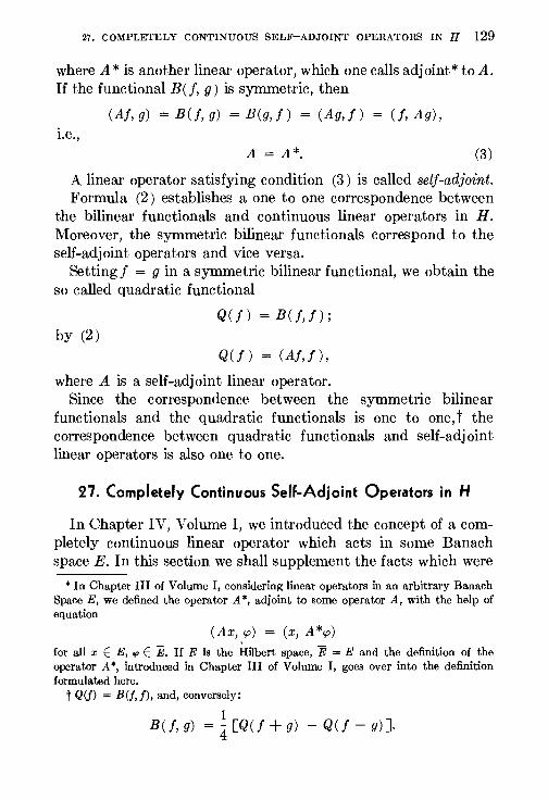
27. COMPLETELY CONTINUOUS SELF-ADJOINT OPERATORS IN H 129
where A* is another linear operator, which one calls adjoint* to A. If the functional B(f, g) is symmetric, then
(Aj, g) = B(f, g) = B(g, f) = (Ag, f) = (f, A g),
i.e., A= A*. (3)
A linear operator satisfying condition (3) is called self-adjoint. Formula (2) establishes a one to one correspondence between
the bilinear functionals and continuous linear operators in H. Moreover, the symmetric bilinear functionals correspond to the self-adjoint operators and vice versa.
Setting f = g in a symmetric bilinear functional, we obtain the so called quadratic functional
Q ( f) = B (f, f) ;
by (2) Q(j) = (Aj,f)'
where A is a self-adjoint linear operator. Since the correspondence between the symmetric bilinear
functionals and the quadratic functionals is one to one, t the correspondence between quadratic functionals and self-adjoint linear operators is also one to one.
27. Completely Continuous Self-Adjoint Operators in H
In Chapter IV, Volume I, we introduced the concept of a completely continuous linear operator which acts in some Banach space E. In this section we shall supplement the facts which were
• In Chapter III of Volume I, considering linear operators in an arbitrary Banach Space E, we defined the operator A*, adjoint to some operator A, with the help of equation
(Ax, cp) = (x, A *cp)
for all x E E, "' E E. If E is the Hilbert space, E = E and the definition of the operator A*, introduced in Chapter III of Volume I, goes over into the definition formulated here.
t Q(j) = B(f,f), and, conversely:
1 B(f, g) = 4 [Q(j +g) - Q(j- g)].
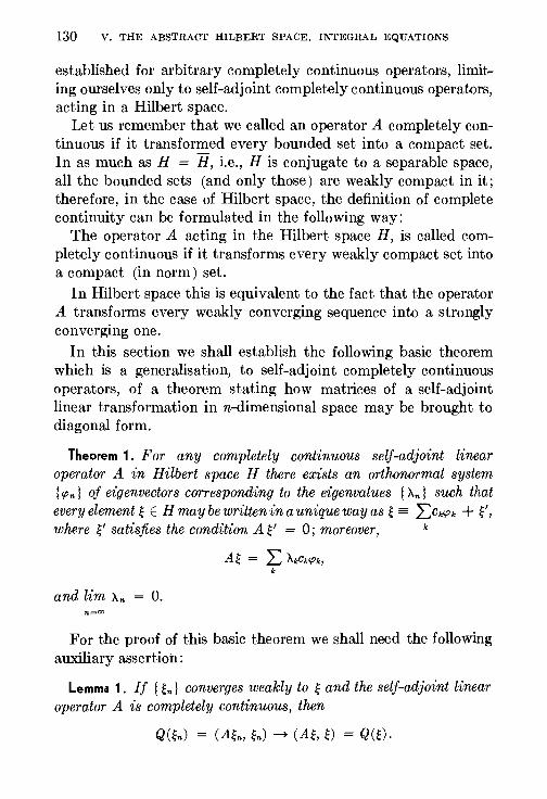
130 V. THE ABSTRACT HILBERT SPACE. INTEGRAL EQUATIONS
established for arbitrary completely continuous operators, limiting ourselves only to self-adjoint completely continuous operators, acting in a Hilbert space.
Let us remember that we called an operator A completely continuous if it transformed every bounded set into a compact set. In as much as H = H, i.e., His conjugate to a separable space, all the bounded sets (and only those) are weakly compact in it; therefore, in the case of Hilbert space, the definition of complete continuity can be formulated in the following way:
The operator A acting in the Hilbert space H, is called completely continuous if it transforms every weakly compact set into a compact (in norm) set.
In Hilbert space this is equivalent to the fact that the operator A transforms every weakly converging sequence into a strongly converging one.
In this section we shall establish the following basic theorem which is a generalisation, to self-adjoint completely continuous operators, of a theorem stating how matrices of a self-adjoint linear transformation in n-dimensional space may be brought to diagonal form.
Theorem 1. For any completely continuous self-adjoint linear operator A in Hilbert space H there exists an orthonormal system I <Pn} of eigenvectors corresponding to the eigenvalues I An} such that every element~ E Hmaybewritteninauniquewayas ~ = L:ck'Pk + e, where e satisfies the condition A e = 0; moreover, k
A~ = L AkCkCf!k, k
and lim An = 0.
For the proof of this basic theorem we shall need the following auxiliary assertion:
Lemma 1. If I ~n} converges weakly to ~ and the self-adjoint linear operator A is completely continuous, then
Q(~n) = (A~n, ~n) ~ (A~, 0 = QW •
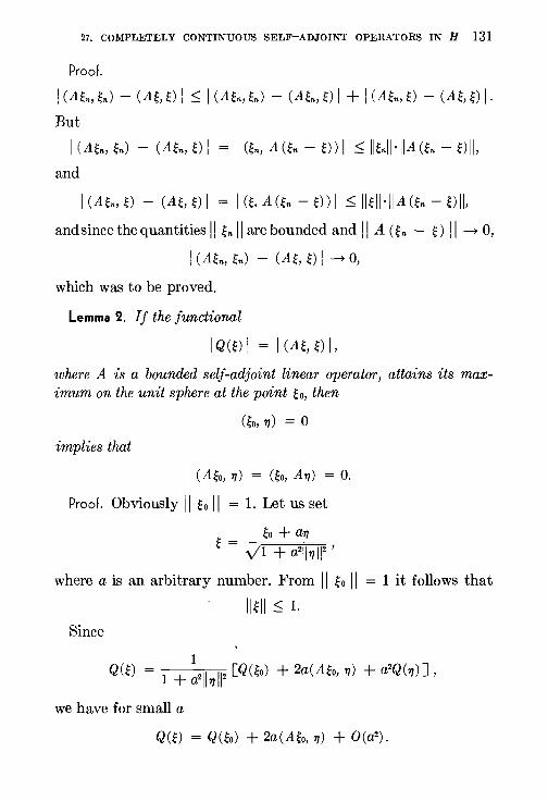
27. COMPLETELY CONTINUOUS SELF-ADJOINT OPERATORS IN H 131
Proof.
I (A~n, ~n) - (A~,~) I :::; I (A~n, ~n) - (A~n, ~)I + I (A~n, ~) - (A~, 0 1. But
I (A~n, ~n) - (A~n, 0 I = I an, A(~n- 0) I :::; ll~nii·IIAan- Oil, and
I (A~n, ~) -(A~,~) I = I(~, A(~n- ~))I :::; II~JI·JIA(~n- Oil, andsincethequantities II ~n II are bounded and II A (~n - ~)II ~ 0,
I (A~n, ~n) - (A~, 0 I ~ 0,
which was to be proved.
Lemma 2. If the functional
IQCO I = I CA~, 0 I, where A is a bounded self-adjoint linear operator, attains its maximum on the unit sphere at the point ~o, then
ao, T/) = 0
implies that
(A~o, 11) = ao, A11) = 0.
Proof. Obviously II ~o II = 1. Let us set
~o + a11 ~ = y1 + a2ll11J!2'
where a is an arbitrary number. From II ~o II = 1 it follows that
II ~II :::; L
Since
we have for small a
Q(O = Q(~o) + 2a(A~o, T/) + O(a2).
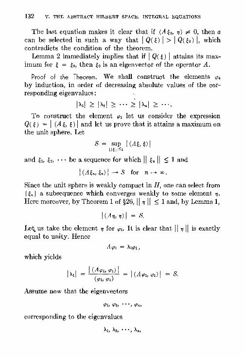
132 V. THE ABSTRACT HILBERT SPACE. INTEGRAL EQUATIONS
The last equation makes it clear that if (A~o, 11) ~ 0, then a can be selected in such a way that I Q( ~) I > I Q( ~o) I, which contradicts the condition of the theorem.
Lemma 2 immediately implies that if I Q( ~) I attains its maximum for ~ = ~o, then ~o is an eigenvector of the operator A.
Proof of the Theorem. We shall construct the elements 'Pk
by induction, in order of decreasing absolute values of the corresponding eigenvalues :
I Ad :2: I A2l :2: " " " :2: I An I :2: • " • •
To construct the element '/'1 let us consider the expression Q( ~) = I (A~' ~) I and let us prove that it attains a maximum on the unit sphere. Let
S = sup I (A~, 0 I 11~11 ~1
and h, b · · · be a sequence for which II ~n II ~ 1 and
I (A~n, ~n) I ~ s for n ~ 00.
Since the unit sphere is weakly compact in H, one can select from { ~n} a subsequence which converges weakly to some element 11·
Here moreover, by Theorem 1 of §26, II 11 II ~ 1 and, by Lemma 1,
ICAT/,1/)I=S.
Le\ us take the element 11 for '/'1· It is clear that II 11 II is exactly equal to unity. Hence
which yields
I A I = I (Acp1, '/'1) I = I (A ) I = s 1 ( ) '/'1, '/'1 .
'/'1, '/'1
Assume now that the eigenvectors
'/'1, '/'21 • • •, <Pn1
corresponding to the eigenvalues
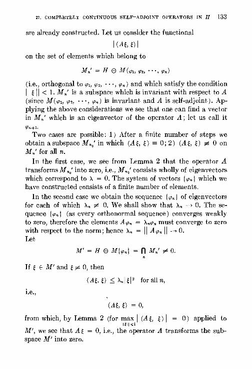
27. COMPLETELY CONTINUOUS SELF-ADJOINT OPERATORS IN H 133
are already constructed. Let us consider the functional
ICA~,~)I
on the set of elements which belong to
Mn' = H 8 M(cp1, '/'2, • • ·, <Pn)
(i.e., orthogonal to cp1, cp2, • • ·, <Pn) and which satisfy the condition )[ ~II< 1. Mn' is a subspace which is invariant with respect to A (since M(cpl, cp2, • • ·, <Pn) is invariant and A is self-adjoint). Applying the above considerations we see that one can find a vector in Mn' which is an eigenvector of the operator A; let us call it 'Pn+l·
Two cases are possible: 1) After a finite number of steps we obtain a subspace Mn.' in which (A~, 0 = 0; 2) (A~, 0 ~ 0 on M n' for all n.
In the first case, we see from Lemma 2 that the operator A transforms M n.' into zero, i.e., M n.' consists wholly of eigenvectors which correspond to A = 0. The system of vectors I <Pn} which we have constructed consists of a finite number of elements.
In the second case we obtain the sequence I <Pn} of eigenvectors for each of which An ~ 0. We shall show that An ~ 0. The sequence I<Pn} (as every orthonormal sequence) converges weakly to zero, therefore the elements Acpn = An<Pn must converge to zero with respect to the norm; hence An = II Acpn II ~ 0. Let
n
If ~ E M' and ~ ~ 0, then
(A~, 0 ~ An)I~W foralln,
I.e.,
(A~,~) = 0,
from which, by Lemma 2 (for max I (A~' ~) I = 0) applied to II Ell :s;l
M', we see that A~ = 0, i.e., the operator A transforms the subspace M' into zero.
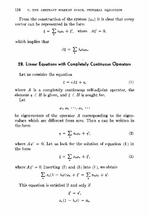
134 V. THE ABSTRACT HILBERT SPACE. INTEGRAL EQUATIONS
From the construction of the system { <Pn} it is clear that every vector can be represented in the form
~ = L Ck'/'k + e, where Ae = o, k
which implies that
28. Linear Equations with Completely Continuous Operators
Let us consider the equation
~ = cA~ + T/, (1)
where A is a completely continuous self-adjoint operator, the element 11 E His given, and ~ E His sought for.
Let
'/'1, '/'2, • • ', 'Pn1 • ' '
be eigenvectors of the operator A corresponding to the eigenvalues which are different from zero. Then 11 can be written in the form
(2)
where A11'
the form 0. Let us look for the solution of equation (1) in
~ = L Xn<Pn + ~1 , n
where A e = 0. Inserting (2) and (3) into (1 ) , we obtain
L Xn(1 - AnC)cpn + e = L an<Pn + T/1
•
n n
This equation is satisfied if and only if
(3)
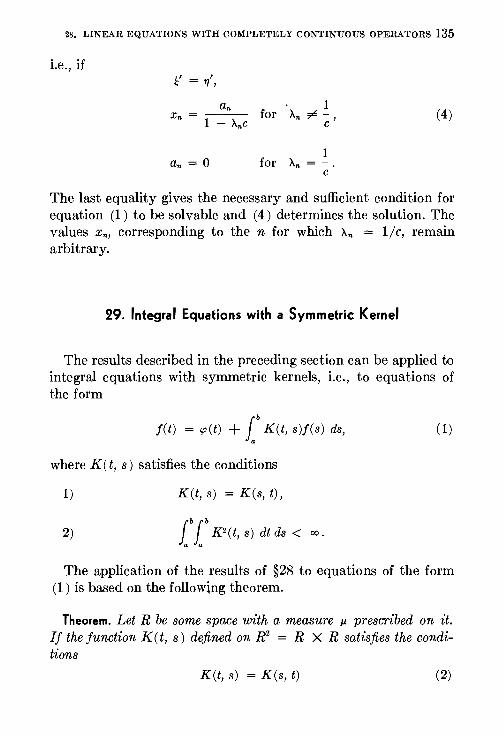
28. LINEAR EQUATIONS WITH COMPLETELY CONTINUOUS OPERATORS 135
i.e., if e = r,',
1 for An = -.
c
(4)
The last equality gives the necessary and sufficient condition for equation (1) to be solvable and (4) determines the solution. The values Xn, corresponding to the n for which An = 1/c, remain arbitrary.
29. Integral Equations with a Symmetric Kernel
The results described in the preceding section can be applied to integral equations with symmetric kernels, i.e., to equations of the form
j(t) = cp(t) + { K(t, s)j(s) ds, a
(1)
where K ( t, s) satisfies the conditions
1) K ( t, s) = K ( s, t) ,
2)
The application of the results of §28 to equations of the form (1) is based on the followlng theorem.
Theorem. Let R be some space with a measure J.L prescribed on it. If the function K ( t, s) defined on R2 = R X R satisfies the conditions
K(t, s) = K(s, t) (2)
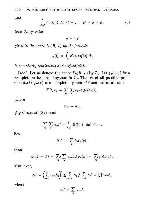
136 V. THE ABSTRACT HILBERT SPACE. INTEGRAL EQUATIONS
and
then the operator
g = Aj,
given in the space L2( R, p.) by the formula
g(t) = l K(t, s)f(s) ds,
is completely continuous and self-adJoint.
(3)
Proof. Let us denote the space L2( R, p.) by L2. Let { ~n( t) } be a complete orthonormal system in L2. The set of all possible products if;n(t) if;m(s) is a complete system of functions in R2
, and
K(t, s) = L L Umnif;n(t)if;m(s)'
where
(by virtue of (2) ) , and
Set
then
Moreover,
where
m n
Umn = Unm
n
n
am2 = I: amn2•
n
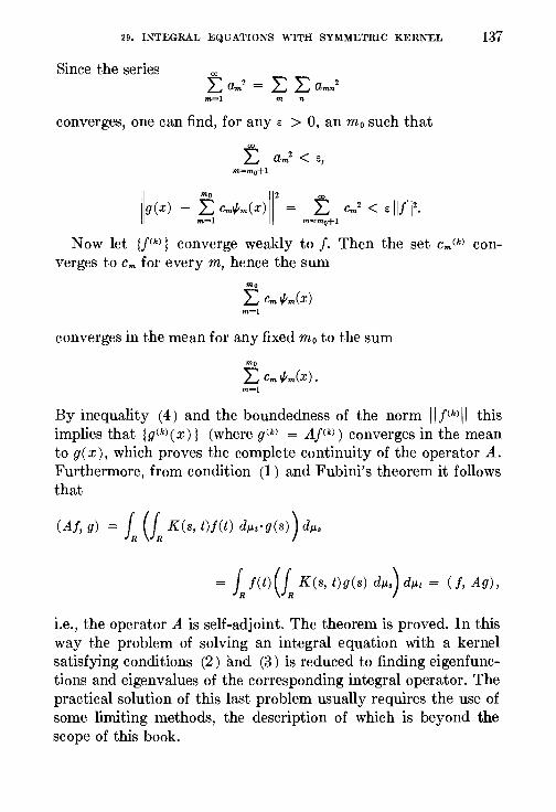
29. INTEGRAL EQUATIONS WITH SYMMETRIC KERNEL 137
Since the series f a,..2 = L L amn2 m=-1 m n
converges, one can find, for any e > 0, an mo such that
Now let lf<k> } converge weakly to f. Then the set Cm <k> converges to Cm for every m, hence the sum
converges in the mean for any fixed mo to the sum
mo
L Cmif;m(X). m=l
By inequality ( 4) and the boundedness of the norm II j<k> II this implies that {g<k>(x)} (where g<k> = Aj<k>) converges in the mean to g( x), which proves the complete continuity of the operator A. Furthermore, from condition (1) and Fubini's theorem it follows that
(Aj, g) = i (i K(s, t)j(t) dp.t•g(s)) dp..
= if(t)(i K(s, t)g(s) dp..)dP.t = (f, Ag),
i.e., the operator A is self-adjoint. The theorem is proved. In this way the problem of solving an integral equation with a kernel satisfying conditions (2) and (3) is reduced to finding eigenfunctions and eigenvalues of the corresponding integral operator. The practical solution of this last problem usually requires the use of some limiting methods, the description of which is beyond the scope of this book.
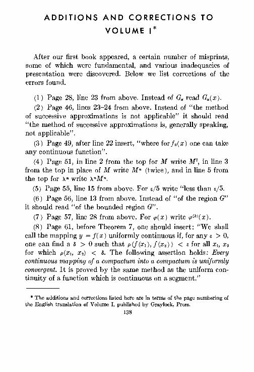
ADDITIONS AND CORRECTIONS TO
VOLUME I*
After our first book appeared, a certain number of misprints, some of which were fundamental, and various inadequacies of presentation were discovered. Below we list corrections of the errors found.
(1) Page 28, line 23 from above. Instead of G,. read Ga(x).
(2) Page 46, lines 23-24 from above. Instead of "the method of successive approximations is not applicable" it should read "the method of successive approximations is, generally speaking, not applicable".
(3) Page 49, after line 22 insert, "where for fo(x) one can take any continuous function".
(4) Page 51, in line 2 from the top for M write M2, in line 3
from the top in place of M write Mn (twice), and in line 5 from the top for >.n write >.nMn.
(5) Page 55, line 15 from above. For e/5 write "less than e/5. (6) Page 56, line 13 from above. Instead of "of the region G"
it should read "of the bounded region G". (7) Page 57, line 28 from above. For cp(x) write cp<k>(x).
(8) Page 61, before Theorem 7, one should insert: "We shall call the mapping y = f( x) uniformly continuous if, for any e > 0, one can find a o > 0 such that p (f (x1), f (x2)) < e for all x1, X2
for which p(x1, x2) < o. The following assertion holds: Every continuous mapping of a compactum into a compactum is uniformly convergent. It is proved by the same method as the uniform continuity of a function which is continuous on a segment."
* The additions and corrections listed here arc in terms of the page numbering of the English translation of Volume I, published by Graylock, Press.
138
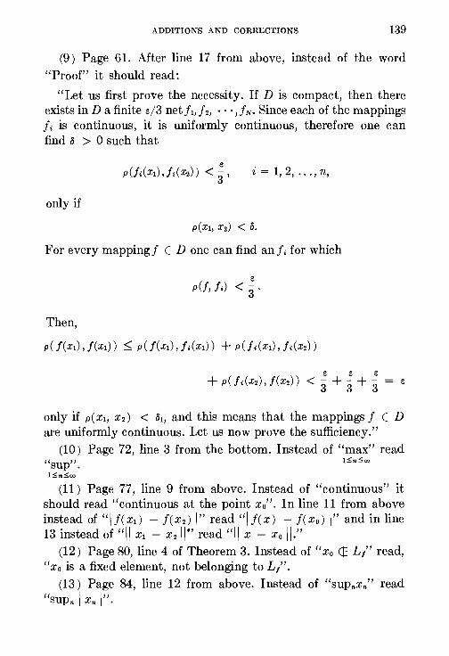
ADDITIONS AND CORRECTIONS 139
(9) Page 61. After line 17 from above, instead of the word "Proof" it should read:
"Let us first pro't'e the necessity. If D is compact, then there exists in D a finite e/3 netj1,j2, · · · ,fN· Since each of the mappings f; is continuous, it is uniformly continuous, therefore one can find o > 0 such that
i=1,2, ... ,n,
only if
p(x1, x2) < o.
For every mapping! E Done can find anf; for which
e p(f, j;) < 3.
Then,
only if p(x1, x2) < o1, and this means that the mappings f E D are uniformly continuous. Let us now prove the sufficiency."
(10) Page 72, line 3 from the bottom. Instead of "max" read "sup". l~n~oo
l::=;:n::=;:oo
(11) Page 77, line 9 from above. Instead of "continuous" it should read "continuous at the point xo". In line 11 from above instead of "IJCx1)- j(x2) I" read "lfCx) - f(xo) I" and in line 13 instead of "II x1 - x2ll" read "II x - Xo II."
(12) Page 80, line 4 of Theorem 3. Instead of "xo EEL/' read, "xo is a fixed element, not belonging to L/'.
(13) Page 84, line 12 from above. Instead of "supnxn" read "supn I Xn I".
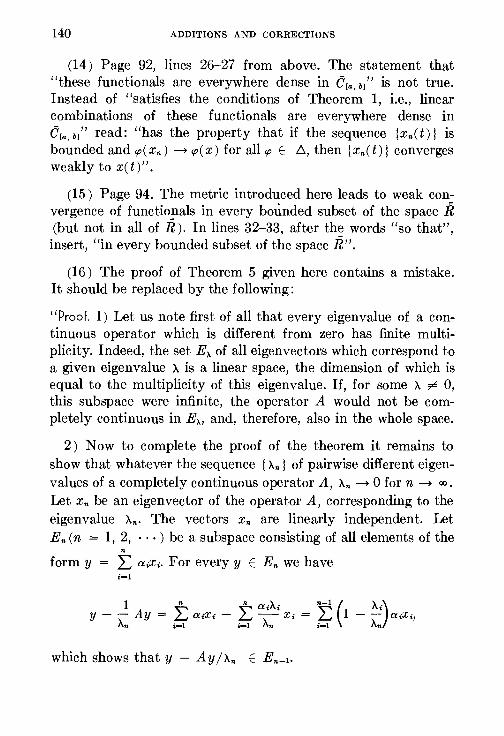
140 ADDITIONS AND CORRECTIONS
(14) Page 92, lines 26-27 from above. The statement that "these functionals are everywhere dense in C[a, b/' is not true. Instead of "satisfies the conditions of Theorem 1, i.e., linear combinations of these functionals are everywhere dense in C[a, bJ" read: "has the property that if the sequence lxn(t)} is bounded and cp( Xn) ~ cp( x) for all cp E 6, then I Xn( t)} converges weakly to x( t)".
(15) Page 94. The metric introduced here leads to weak convergence of functionals in every bounded subset of the space R (but not in all of R ). In lines 32-33, after the words "so that", insert, "in every bounded subset of the space R".
(16) The proof of Theorem 5 given here contains a mistake. It should be replaced by the following:
"Proof. 1) Let us note first of all that every eigenvalue of a continuous operator which is different from zero has finite multiplicity. Indeed, the set Ex of all eigenvectors which correspond to a given eigenvalue A is a linear space, the dimension of which is equal to the multiplicity of this eigenvalue. If, for some A ~ 0, this subspace were infinite, the operator A would not be completely continuous in Ex, and, therefore, also in the whole space.
2) Now to complete the proof of the theorem it remains to show that whatever the sequence I An} of pairwise different eigenvalues of a completely continuous operator A, An ~ 0 for n ~ oo.
Let Xn be an eigenvector of the operator A, corresponding to the eigenvalue An· The vectors Xn are linearly independent. Let En (n = 1, 2, · · ·) be a subspace consisting of all elements of the
n
form y = I: a;X,:. For every y E En we have i=l
which shows that y - Ay /An E En-1·
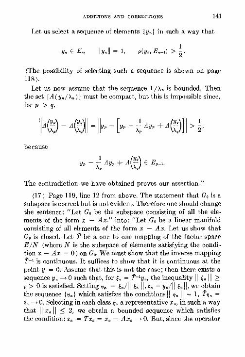
ADDITIONS AND CORRECTIONS 141
Let us select a sequence of elements { Yn} in such a way that
IIYnll = 1,
(The possibility of selecting such a sequence is shown on page 118).
Let us now assume that the sequence 1 I An is bounded. Then the set {A(Ynl>-n)} must be compact, but this is impossible since, for p > q,
because
The contradiction we have obtained proves our assertion."
(17) Page 119, line 12 from above. The statement that Go is a ~ubspace is correct but is not evident. Therefore one should change the sentence: "Let Go be the subspace consisting of all the elements of the form x - Ax." into: "Let Go be a linear manifold consisting of all elements of the form x - Ax. Let us show that Go is closed. Let T be a one to one mapping of the factor space E IN (where N is the subspace of elements satisfying the condition x- Ax = 0) on Go. We must show that the inverse mapping T-1 is continuous. It suffices to show that it is continuous at the point y = 0. Assume that this is not the case; then there exists a sequence Yn ~ 0 such that, for ~n = T-1yn, the inequality II ~n II ;:::: p > 0 is satisfied. Setting 11~> = ~nil I ~n II, Zn = Ynlll ~n II, we obtain the sequence {Tin} which satisfies the conditions II T/n II = 1, TT/n = Zn ~ 0. Selecting in each class Tin a representative Xn, in such a way that II Xn II ~ 2, we obtain a bounded sequence which satisfies the condition: Zn = Txn = Xn - Axn ~ 0. But, since the operator
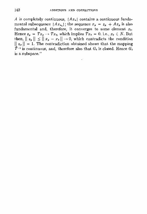
142 ADDITIONS AND CORRECTIONS
A is completely continuous, {Axn} contains a continuous fundamental subsequence { Axnk}; the sequence Xp = Zp + Axp is also fundamental and, therefore, it converges to some element xo. Hence Zp = TxP ~ Tx 0, which implies Txo = 0. i.e., x 0 E N. But then, II T/p II ~ II Xp - Xo II ~ 0, which contradicts the condition II T/p II = 1. The contradiction obtained shows that the mapping T-1 is continuous, and, therefore also that Go is closed. Hence Go is a subspace."
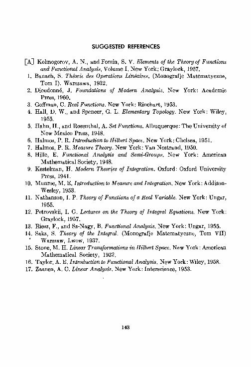
SUGGESTED REFERENCES
[A] Kolmogorov, A. N., and Fomin, S. V. Elements of the Theory of Functions and Functiorwl Arwlysis, Volume I. New York: Graylock, 1957.
1. Banach, S. Theorie des Operations Lineaires. (Monografje Matematyczne, Tom I). Warszawa, 1932.
2. Dieudonne, J. Foundations of Modern Arwlysis. New York: Academic Press, 1960.
3. Goffman, C. Real Functions. New York: Rinehart, 1953. 4. Hall, D. W., and Spencer, G. L. Elementary Topology. New York: Wiley,
1955. 5. Hahn, H., and Rosenthal, A. Set Functions. Albuquerque: The University of
New Mexico Press, 1948. 6. Halmos, P.R. Introduction to Hilbert Space. New York: Chelsea, 1951. 7. Halmos, P.R. Measure Theory. New York: Van Nostrand, 1950. 8. Hille, E. Functional Arwlysis and Semi-Groups. New York: American
Mathematical Society, 1948. 9. Kestelman, H. Modern Theorles of Integration. Oxford: Oxford University
Press, 1941. 10. Munroe, M. E. Introduction to Measure and Integration. New York: Addison
Wesley, 1953. 11. Nathanson, I. P. Theory of Functions of a Real Variable. New York: Ungar,
1955. 12. Petrovskii, I. G. Lectures on the Theory of Integral Equations. New York:
Graylock, 1957. 13. Riesz, F., and Sz-Nagy, B. Functiorwl Arwlysis. New York: Ungar, 1955. 14. Saks, S. Theory of the Integral. (Monografje Matematyczne, Tom VII)
' Warszaw, Lwow, 1937. 15. Stone, M. H. Lirmar Transformations in Hilbert Space. New York: American
Mathematical Society, 1932. 16. Taylor, A. E. Introduction to Functional Arwlysis. New York: Wiley, 1958. 17. Zaanen, A. C. Lirmar Analysis. New York: Interscience, 1953.
143

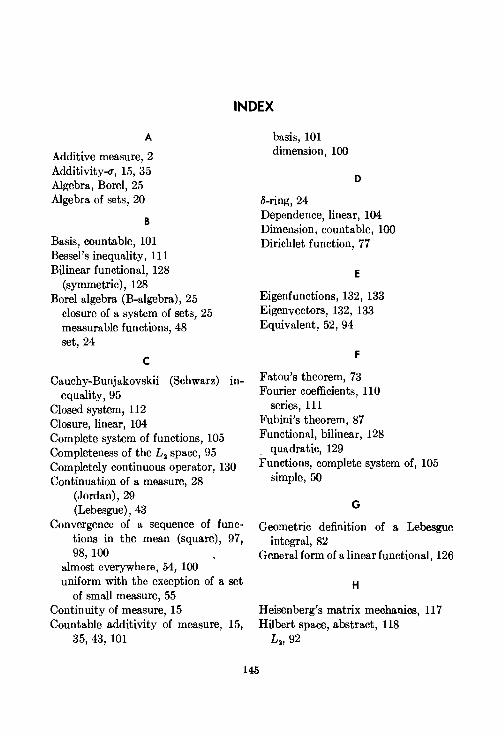
INDEX
A
Additive measure, 2 Additivity-a, 15, 35 Algebra, Borel, 25 Algebra of sets, 20
8
Basis, countable, 101 Bessel's inequality, 111 Bilinear functional, 128
(symmetric), 128 Borel algebra (B-algebra), 25
closure of a system of sets, 25 measurable functions, 48 set, 24
c Cauchy-Bunjakovskii (Schwarz) in-
equality, 95 Closed system, 112 Closure, linear, 104 Complete system of functions, 105 Completeness of the L2 space, 95 Completely continuous operator, 130 Continuation of a measure, 28
(Jordan), 29 (Lebesgue), 43
Convergence of a sequence of functions in the mean (square), 97, 98, 100
almost everywhere, 54, 100 uniform with the exception of a set
of small measure, 55 Continuity of measure, 15 Countable additivity of measure, 15,
35, 43, 101
basis, 101 dimension, 100
o-ring, 24
D
Dependence, linear, 104 Dimension, countable, 100 Dirichlet function, 77
E
Eigenfunctions, 132, 133 Eigenvectors, 132, 133 Equivalent, 52, 94
F
Fatou's theorem, 73 Fourier coefficients, 110
series, 111 Fubini's theorem, 87 Functional, bilinear, 128
quadratic, 129 Functions, complete system of, 105
simple, 50
G
Geometric definition of a. Lebesgue integral, 82
General form of a linear functional, 126
H
Heisenberg's matrix mechanics 117 Hilbert space, abstract, 118 '
L 2, 92
145
146 INDEX
Independence, linear, 104 Integrable, 61, 63 Integral, as a set function, 90
equation with symmetric kernel, 135 operator, 123
Inner measure, 6, 31, 40 Isomorphic spaces, 115 Isomorphism of L, and l, spaces, 115
L
Lebesgue integral, 63, 76, 106 measurable set, 7, 40, 45 non-measurable set, 18
Lebesgue-Stieltjes measure, 17 Limiting process under Lebesgue inte
gral sign, 69 Linear closure, 105
manifold, 121 self-adjoint operator, 129
Linearly independent system of func-tions, 104
closed system of functions, 112 complete system of functions, 105 normalised system of functions, 106 orthogonal system of functions,
106, 107 Luzin's theorem, 53
M
Manifold, linear, 121 Measurable function, 48, 49 Measure of a set, 26
absolutely convergent, 26 complete, 46 continuity of, 15 discrete, 18 inner, 6, 31, 40 Jordan, 30 Lebesgue, 7, 40 Lebesgue-Stieltjes, 17 singular, 17 with countable basis, 101
Minimal ring, 21 Mutually orthogonal, 106
N
Nonseparable Hilbert space, 119 Normalised system, 106
0
Orthogonal complement to subspace, '123
mutually, 106 Orthogonalisation of a system of
vectors (functions), 109 Orthonormal system, 106 Outer measure, 6, 31, 40
p
Parseval's equation, 112 Plane measure and linear measure, 82 Power, nth of a set, 78 Product of measures, 82
vector, 94
Q
Quadratic functional, 129
R
Radon's theorem, 90 Riemann integra.! (comparison), 75 Riesz-Fischer theorem, 113 Ring of sets, 19
its unit, 19 minimal, 21, 24
s
IT-additivity, 15, 35 er-ring, 19 Scalar product, 94 Schrodinger's wave mechanics, 117 Schwarz inequality, 95 Self-adjoint linear operator, 129 Semiring, 21
Set, algebra of, 20 B-closure, 25 function, 90 measurable, 40 of unique measure, 44
Simple functions, 50 Square integrable, 93 Subspace of Hilbert space, 121 Summable, 93
T
Tchebishev's inequality, 68
INDEX 147
u
Uniqueness, set of, 38 Unit of system of sets, 19, 39 Unit sphere, weak compactness, 127
v Vector product, 94
w Weak compactness of unit sphere, 127
Related Documents
![[Madan Lal Mehta] Random Matrices(BookFi-2](https://static.cupdf.com/doc/110x72/54520983b1af9f7a248b4c20/madan-lal-mehta-random-matricesbookfi-2.jpg)


![[Fomichenko L.G.] Speaking Clearly. Improving Voic(BookFi)](https://static.cupdf.com/doc/110x72/577c84731a28abe054b901d3/fomichenko-lg-speaking-clearly-improving-voicbookfi.jpg)

![[Rumi, Deepak Chopra, Fereydoun Kia] the Love Poem(BookFi)](https://static.cupdf.com/doc/110x72/577c78491a28abe0548f7192/rumi-deepak-chopra-fereydoun-kia-the-love-poembookfi.jpg)


![[Tarasenko F.P.] Prikladnoi sistemnuei analiz(BookFi)library.fa.ru/files/Tarasenko.pdf · Title [Tarasenko_F.P.]_Prikladnoi_sistemnuei_analiz(BookFi).djvu Author: Ermilova Created](https://static.cupdf.com/doc/110x72/5f5ba63e2f46196f607ab9b2/tarasenko-fp-prikladnoi-sistemnuei-analizbookfi-title-tarasenkofpprikladnoisistemnueianalizbookfidjvu.jpg)