A multiplicatively-weighted Voronoi diagram approach to logistics districting

Computers & Operations Research 33 (2006) 93–114

www.elsevier.com/locate/cor

A multiplicatively-weighted Voronoi diagram approach tologistics districting

Lauro C. Galvãoa, Antonio G.N. Novaesb,∗, J.E. Souza de Cursic, João C. Souzab

aCEFET-PR, Av. Sete de Setembro 3165, Curitiba, PR, 80230-901, BrazilbFederal University of Santa Catarina, Caixa Postal 476, Florianópolis, SC, 88010-970, Brazil

cINSA de Rouen, Av. de l’Université, 76801 Saint Etienne du Rouvray CEDEX, France

Available online 20 August 2004

Abstract

The objective of districting in logistics distribution problems is to find a near optimal partition of the servedregion into delivery zones or districts. This kind of problem has been treated in the literature with geometric-shaped districts and continuous approximations. Usually it is assumed an underlying road network equivalentto a Euclidean, rectangular, or ring-radial metric. In most real problems, however, the road network is a coarsecombination of metrics. In this context, it is unclear what is the optimal shape of the districts and how one shouldorientate them. A possibility is to treat the problem with a Voronoi diagram approach. Departing from a previouslydetermined ring-radial districting pattern and relaxing the initial district boundaries, we apply the multiplicatively-weighted Voronoi diagram formulation in order to smooth district contours. The computing process is iterated untilthe convergence is attained. The model has been applied to solve a parcel delivery problem in the city of São Paulo,Brazil, whose results are presented and discussed in the paper.� 2004 Elsevier Ltd. All rights reserved.

Keywords:Districting; Distribution; Voronoi diagram

1. Introduction

In districting problems, the aim is to partition a territory into smaller units, called districts or zones,subject to some side constraints[1]. Usually the constraints reflect a number of common sense criteria.One of them is equality, i.e., the number of elements in any district must lie within a predetermined

∗ Corresponding author. Tel.: + 55-48-331-7009; fax: 55-48-331-7075.E-mail address:[email protected](A.G.N. Novaes).

0305-0548/$ - see front matter� 2004 Elsevier Ltd. All rights reserved.doi:10.1016/j.cor.2004.07.001

http://www.elsevier.com/locate/cor

mailto:[email protected]

94 L.C. Galvão et al. / Computers & Operations Research 33 (2006) 93–114

range. In addition, the resulting districts must be contiguous and geographically compact[2]. There isno consensus, however, on which criteria are legitimate and on how these should be measured[3,1]. Aspointed out by Guo et al.[4], the criteria on what constitutes a meaningful districting procedure lie in thepurpose of the studies and rely on the district designer to define.

Districting problems are associated with a number of planning processes. For example, when dealingwith spatial/geographical information, it is often necessary to investigate a set or subset of spatial objectattributes in order to assess cluster presence. As a literature review suggests, there is a wide range ofdistricting applications. Political districting, in which one is interested in drawing of electoral districtboundaries[5,2] has received much attention in the literature. A review on political districting is encoun-tered in[3], and an up-to-date bibliography on the subject is reported in[1]. School districting[6] andpolice districting[7] are two other areas of research interest. In addition, the literature presents articleson the design of sales territory[8], as well as emergency, health-care, and logistics districting. Amongthe latter we mention the districting approach to the planning of salt spreading operations on roads[9],the balanced allocation of customers to distribution centers[10], and the design of multi-vehicle deliverytours[11–16].

Most of districting problems are solved with a discrete mathematical programming model. The arealunits are grouped into a number of districts such that some function is optimized, subject to additionalconstraints. This kind of problem has been proved to be NP-hard, meaning that the computational effortrequired for finding the optimal solution grows exponentially as the problem size increases. Continuousapproximations, on the other hand, are based on the spatial density and distribution of the demand ratherthan on precise information on every demand point. These continuous approximations allow simple,yet robust models that are useful when planning a new service or the expansion of an existing one[16–19]. A number of freight-distribution districting problems have been solved with this approach[11,12,14,16,20].

Assuming an underlying ring-radial network centered at the source (depot), Newell and Daganzo[12]pointed out that for regions in which the number of zones is relatively large, there should be some patternof concentric rings of districts around the source. A number of continuous models of freight distributionshow a ring-radial partition pattern[11,12,20,16]. The continuous ring-radial metric is, in fact, quiteartificial [13]. Most real road networks display a somewhat complex hierarchy of arterials, freeways, etc,together with a local grid geometry. Newell and Daganzo[13] analyzed possible districting schemes forsome other road patterns, showing that the resulting geometry for the zones may be quite different thanfor the dense ring-radial network previously studied in[12]. In the real world, most cities neither showa ring-radial road network pattern, nor a strictL1 (grid) or L2 (Euclidean) metric. In this context, it isunclear what is the optimal shape of the districts and how one should orientate them. A possibility is totreat the problem as a Voronoi diagram, as we do in this paper.

Departing from a geometrically-shaped districting pattern, such as a ring-radial partition, (see Novaeset al. [16]), one can smooth district contours with the aid of a Voronoi diagram[21–24]. The Voronoidiagram is a very simple diagram. Given a set of a finite number (two or more) of distinct points inthe Euclidean plane, one associates all locations on that space with the closest member(s) of the pointset with respect to the Euclidean distance[22]. We use in this paper a special case of Voronoi diagram,the multiplicatively-weighted (MW-) Voronoi diagram[21], combined with an iterative computationalprocedure to solve an urban freight distribution problem.

A problem similar to the one analyzed in this paper was treated differently by Langevin and Saint-Mleux [14]. They adopted an underlying continuous approximation model as we do in this paper. But

L.C. Galvão et al. / Computers & Operations Research 33 (2006) 93–114 95

instead of employing an automated districting process, they developed a decision support system thatenables the distribution manager to interactively design the districts by inspection. In our formulationone departs from a previous geometrically shaped optimal solution and the system automatically definesthe district contours with the aid of a Voronoi diagram.

The utilization of MW-Voronoi diagrams in logistics districting has some advantages. First, the fittingprocess leads to more equalized load factors among the districts, meaning the vehicles assigned to thezones will show more balanced utilization levels. This happens because the MW-Voronoi diagram hasmore degrees of freedom when searching for the district contours. Second, this approach opens the wayto incorporate physical barriers into the model[25]. This is an important property because it permits thehandling of problems with obstacles imposed by thoroughfares, highways, rivers, reservoirs, hills, etc.The extension of the model to incorporate obstacles will be the subject of another paper.

Of course, when one departs from the ring-radial solution as adopted in[11,12,15,16,20], some costpenalty will be imposed to the solution, albeit small in most cases. But, regarding the significant depar-tures from the theoretical modeling framework frequently observed when solving real-world problems(irregular road networks, varying traffic constraints, sub-optimal routing strategies, etc), the resulting costpenalty might be regarded, in most cases, as imbedded in the overall approximation error.

In order to verify possible cost penalties when adopting the MW-Voronoi diagram format, a series ofstatistical tests was performed, comparing alternate districting configurations with the ring-radial solu-tion (see Section 6.3). Although square and circular-shaped districts always presented average travelingdistances greater than the equivalent wedge-shaped ones, the same did not always occur to the MW-Voronoi-diagram zones. When the Voronoi zones are more elongated toward the depot and located fartherfrom it, as zone 74 inFig. 6, the average traveling distance per point tend to be smaller than the corre-sponding wedge-shaped configuration. On the other hand, districts located closer to the depot and notelongated toward it, as zone 23 inFig. 6, tend to show average traveling distances greater than the equiv-alent wedge-shaped zones. The differences are small, however, and the positive and negative variationstend to partially balance. For the case reported in this paper, the average traveling distance for the MW-Voronoi diagram configuration shown inFig. 6was only 0.26% greater than the original wedge-shapedconfiguration (see Section 6.3).

In Section 2 of the paper and in the Appendix we briefly indicate how we approximate continuousfunctions to spatial discrete variables such as the number of served points, the quantity of product tobe delivered, and the stopping times. Section 3 describes the preliminary ring-radial districting solution,obtained from[16], and used as a basis to apply MW-Voronoi diagram process, which is the mainobjective of this paper. In Section 4 we discuss, in general terms, the possible effects of the road networkcharacteristics on the shape and orientation of the districts. In Section 5, the Voronoi diagram fittingprocess is described and analyzed. Finally, Section 5.3 is dedicated to describe the computational aspectsof the problem and the results.

2. Continuous demand approximation

A number of transportation and logistics problems can be converted into problems involving continuousfunctions, with good practical results. Continuous demand approximation models are based on the spatialdensity and distribution of the demand rather than on precise information on every demand point. Thesecontinuous approximations allow simple, yet robust models that are useful when planning a new service


or the expansion of an existing one[17–19]. A number of freight-distribution districting problems havebeen solved with this approach[11,12,14,16,20].

Let Sbe a generic sub-region of the served regionR. Demand is expressed by three variables: (a) thenumber of points (customers) inS; (b) the total quantity of product to be delivered inS; (c) the totalstopping time spent inS. Assuming a Cartesian system of coordinates, letf (x, y) generically representone of those variables. We introduce a bi-dimensional cumulative function

F(S) =∫S

f (x, y)dx dy. (1)

Then, we approximate a continuous function toF(S) as to have suitable mathematical properties ofdifferentiability. In this work the approximation is attained with a bi-quadratic spline[26,27], combinedwith a finite element discretization[28,29]of regionR. Our choice is due to the fact that the optimizationprocedure employed in this paper implies repeated numerical evaluations of Eq. (1). Supplementaryelements are presented in the Appendix.

3. A preliminary ring-radial partitioning solution

3.1. Background

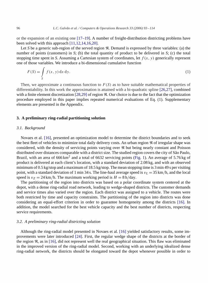
Novaes et al.[16], presented an optimization model to determine the district boundaries and to seekthe best fleet of vehicles to minimize total daily delivery costs. An urban regionR of irregular shape wasconsidered, with the density of servicing points varying overR but being nearly constant and Poissondistributed over distances comparable with a district size. The studied region covers the city of São Paulo,Brazil, with an area of 666 km2 and a total of 6632 servicing points (Fig. 1). An average of 5.76 kg ofproduct is delivered at each client’s location, with a standard deviation of 2.08 kg, and with an observedminimum of 0.5 kg/stop and a maximum of 18.5 kg/stop. The mean stopping time is 3 min 49 s per visitingpoint, with a standard deviation of 1 min 34 s. The line-haul average speed isvL =35 km/h, and the localspeed isvZ = 24 km/h. The maximum working period isH = 8 h/day.

The partitioning of the region into districts was based on a polar coordinate system centered at thedepot, with a dense ring-radial road network, leading to wedge-shaped districts. The customer demandsand service times also varied over the region. Each district was assigned to a vehicle. The routes wereboth restricted by time and capacity constraints. The partitioning of the region into districts was doneconsidering an equal-effort criterion in order to guarantee homogeneity among the districts[16]. Inaddition, the model searched for the best vehicle capacity and the best number of districts, respectingservice requirements.

3.2. A preliminary ring-radial districting solution

Although the ring-radial model presented in Novaes et al.[16] yielded satisfactory results, some im-provements were later introduced[24]. First, the regular wedge shape of the districts at the border ofthe regionR, as in[16], did not represent well the real geographical situation. This flaw was eliminatedin the improved version of the ring-radial model. Second, working with an underlying idealized densering-radial network, the districts should be elongated toward the depot whenever possible in order to


Fig. 1.

reduce the line-haul segments of the routes[12]. By inspection, the ill-shaped districts were changed intodistricts elongated toward the depot. Third, in order to keep district slenderness[15,16]within reasonablelimits, appropriate lower and upper restrictions were imposed.

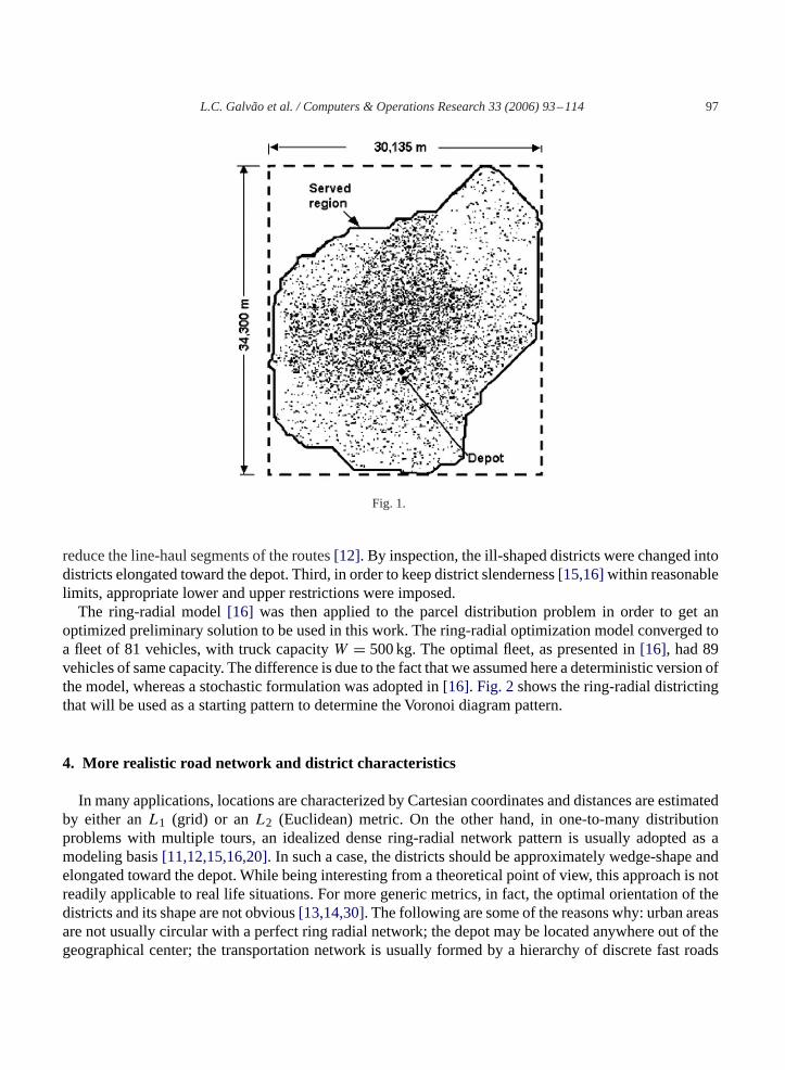
The ring-radial model[16] was then applied to the parcel distribution problem in order to get anoptimized preliminary solution to be used in this work. The ring-radial optimization model converged toa fleet of 81 vehicles, with truck capacityW = 500 kg. The optimal fleet, as presented in[16], had 89vehicles of same capacity. The difference is due to the fact that we assumed here a deterministic version ofthe model, whereas a stochastic formulation was adopted in[16]. Fig. 2shows the ring-radial districtingthat will be used as a starting pattern to determine the Voronoi diagram pattern.

4. More realistic road network and district characteristics

In many applications, locations are characterized by Cartesian coordinates and distances are estimatedby either anL1 (grid) or anL2 (Euclidean) metric. On the other hand, in one-to-many distributionproblems with multiple tours, an idealized dense ring-radial network pattern is usually adopted as amodeling basis[11,12,15,16,20]. In such a case, the districts should be approximately wedge-shape andelongated toward the depot. While being interesting from a theoretical point of view, this approach is notreadily applicable to real life situations. For more generic metrics, in fact, the optimal orientation of thedistricts and its shape are not obvious[13,14,30]. The following are some of the reasons why: urban areasare not usually circular with a perfect ring radial network; the depot may be located anywhere out of thegeographical center; the transportation network is usually formed by a hierarchy of discrete fast roads


Fig. 2.

(arterials, freeways), together with local streets showing irregular arrangements, etc. The theory may benevertheless be used as a guideline in the construction of the delivery districts to avoid gross sub optimalchoices[14].

Newell and Daganzo[13] analyzed some more realistic geometries of roads. First, they suggest that,for any geometry of roads, one should first construct a family of equi-travel-time contours from thesource (depot), via fastest routes. If there are fast roads irradiating from the source to the periphery, thezones having access from these fast roads should be elongated approximately along the ring directions.Obviously one must go out quite some distance from the origin before one can start packing zoneselongated in the ring direction. On the other hand, those districts having access from the secondaryradials should be elongated in the radial direction[13]. In some large cities, however, traffic congestionschange the flowing conditions on a day-to-day basis. As a consequence, truck drivers usually try differentpaths to and from the delivery zones according to traffic reports.

Other authors[31,32] have tried to approximate distances with modified norms. In particular, theweighted�p norm with axis rotation[31] combinesL1 (grid) andL2 (Euclidean) metrics into oneunique representation. The weighted�p norm can be applied when the road network has part of its linksapproximately parallel or orthogonal to a direction defined by an angle� with the Cartesian coordinateaxis. The weighted�p norm with axis rotation is defined as[31]

�p(i, j) = k[ ∣∣xi − xj

∣∣p + ∣∣yi − yj

∣∣p]1/p, (2)


wherek >0 is the route impedance,p >1, and{xq, yq} are the transformed coordinates of a generic pointq, given by

[xq yq] = [x0q y0

q ][

cos� − sin�sin� cos�

], (3)

where{x0q , y0

q} are the original coordinates ofq.In order to fit the weighted�p norm (2) to a region, one has to take a sufficient large number of locations

over the network and determine the shortest road distancedbetween each pair of points. Then, a computerprogram will vary�, p, andk in order to fit�p to the values ofd so as to optimize a global pre-selectedcriterion[31]. This fitting process was applied to three sub-regions of the city of Sao Paulo, Brazil, withareas of 0.7, 9.8 and 18.4 km2, respectively. Ap-value close to 2 implies that distances are essentiallyL2(Euclidean), multiplied by a route factor. Otherwise, whenp is close to 1, the result implies that distancesare better explained by aL1 (grid) metric. For the smallest sub-region, a valuep = 1.95 was obtained,meaning the road network metric is essentially Euclidean. The values ofp, for the two other sub-regions,were 1.22 and 1.29, respectively, meaning the underlying geometry is closer to the rectangular metric.The fitted angle�, on the other hand, varied significantly from 45◦17′ to 73◦34′, indicating that there isnot a predominant lattice direction that might justify the adoption of an uniqueL1 (rectangular) metric.Thus, for the case studied in this paper, we conclude there is not a predominant metric that could serveas the basis for the local network geometry.

The indefinition of the local network metric makes the ideal shape of the zones unclear. Furthermore,since the real transportation infrastructure presents a coarse network of fast roads with varying velocity ona day-to-day basis, the ideal orientation of the districts is also unclear[13]. In particular, a MW-Voronoidiagram partitioning scheme is a possible districting criterion. We will see in Sections 5.7 and 5.6 that,although the Voronoi diagram partitioning process will change the shape of the districts, also changingin a minor scale their orientation, the resulting total distribution cost is only marginally affected.

5. Voronoi diagram fitting to the logistics districting problem

5.1. Multiplicatively-weighted Voronoi diagrams

Voronoi diagrams have been extensively used in a variety of disciplines. The concept of an ordinarydiagram is quite simple: given a finite set of distinct, isolated points in a continuous space, we associateall locations in that space with the closest member of a set of points(P1,P2, . . . ,Pm) [21]. There aresituations where the Euclidean distance does not represent well the attracting process. For instance, theMW-Voronoi diagram inR2 is defined by connecting the set of points with a set of strictly positive weightsw = (w1, w2, . . . , wm). The MW-Voronoi polygon associated withPi is [21]

V (Pi) ={X ∈ R2

∣∣∣∣ 1

wi

‖X − Pi‖ �1

wj

∥∥X − Pj

∥∥ , j = i, j = 1, . . . , m

}, (4)

where‖•‖ is the Euclidean norm

‖P‖ =√

P 21 + P 2

2 ; P= (P1, P2). (5)


In the case with only two generator points, the locus of the pointsX satisfying (4) is the Apollonius circle[21], except ifw1 = w2, when the bisector becomes a straight line. In general, a MW-Voronoi region is anon-empty set and needs not be convex or connected. In particular, it may have holes.

The main reason for adopting aVoronoi-diagram approach to logistics districting, as we have done here,is the possibility of further employing some of its properties to get better approximations to real-worldproblems.

5.2. Vehicle cycle approximation

Here one is not interested in directly finding the best sequence of visiting points for each tour. Ap-proximate formulas are used to estimate the traveled distances, and the effort is concentrated in seeking anear optimal partition of the served region into districts. The expected distanceDZ traveled by a vehiclewithin a district of areaA andn visiting points can be approximated as[33,20,16]

DZ ≈ k0√

An. (6)

Expression (6) can be applied to most metrics and presupposes that the points are uniformly andindependently scattered over the area, that an optimum traveling salesman tour has been drawn to coverthen points in question, and the district is fairly compact and fairly convex[33]. The coefficientk0 canbe expanded into two multiplicative factors

k0 = k1k2. (7)

The value ofk1 depends solely on the adopted metric and routing strategy. For the classical travelingsalesman problem (TSP) andL2 metric, for instance, one hask1 = 0.765, which gives reasonable resultsfor n>15, holding quite well for different district shapes[33]. The factork2 is a corrective coefficient(route factor) reflecting the road network impedance. Its value depends on the local road network structureand traffic regulations. We adoptedk2 = 1.35 in our computations, as in[15].

The vehicle starts from the depot, goes to the assigned district, does the delivery, and comes back tothe depot when all visits are completed. This complete sequence makes up the vehicle cycle. Admittinga total ofm daily tours, the total cycle lengthLi of routei (i = 1,2, . . . , m) is the sum of the line-hauldistance (either way) and the local travel distance given by (6). The total cycle timeTi , on the other hand,is the sum of the line-haul time, the local travel and the total handling time. The latter is the integralF

(s)i

of the stopping times spent in delivering the cargo at the customer’s locations within the districti (seeSection 2). The expected value ofTi , for a generic touri, is

Ti = 2D(LH)i

vL

+ k0√

Ai ni

vZ

+ F(s)i , (8)

whereD(LH)i is the expected line-haul travel distance (one way) from the depot to the districti, vL is the

average line-haul speed, andvZ is the average local speed. IfH is the maximum daily working time, then

Ti � H for i = 1,2, . . . , m. (9)


Let F (q)i be the integral of the quantities of cargo delivered at the visiting points located in the district

i. Then, the total cargo carried by the vehicle serving districti, is

Qi = F(q)i . (10)

If W is the vehicle loading capacity , then

Qi �W for i = 1,2, . . . , m. (11)

5.3. Equalization of the distributing effort

One common objective of most districting problems is to attain a certain level of equality among thedistricts. The equality refers to some specific variables describing the districts, which can be generallytreated as a measure of the size of the zone or, as in the case analyzed in this paper, a measure of the effortexerted to perform the service.

The distribution service along routei may be constrained by working time or loading capacity, depend-ing on what restriction (9) or (11) is binding. Instead of introducing restrictions (9) and (11) directly intothe model, we introduced two load factors, the first taking into account time utilization and, the second,truck capacity utilization

�(T )i = Ti

H�1 and �(Q)

i = Qi

W�1, i = 1,2, . . . , m. (12)

For each district the system compares�(T )i and�(Q)

i , selecting the largest value to represent the districtload factor:

�i = max{�(T )i ,�(Q)

i }. (13)

At each stage of the iterative process, the system analyzes the vector�=(�1, . . . ,�m) and computes themaximum load factor max(�)=max{�1, . . . ,�m}, the minimum load factor min(�)=min{�1, . . . ,�m},the average load factora(�) and the mean quadratic deviations(�):

a(�) = 1

m

m∑i=1

�i , s(�) =(

1

m

m∑i=1

(�i − a(�))2

)1/2

. (14)

We observe that, on the one hand, the load factor has the same value for all the districts if and only ifs(�) is zero, and, on the other hand, that conditions (12) are satisfied if and only if max(�) is not greaterthan unity. So, the regionR is partitioned into perfectly homogeneous districts respecting the time andcapacity limitations when

s(�) = 0, max(�)�1. (15)

Although ideallys(�) = 0 and max(�) = 1, it is convenient to consider, in practice, a small toleranceε >0 furnished by the user. Thus, we consider that the regionR is partitioned into homogeneous districtswhens(�)�ε; 1 − ε� max(�)�1. These conditions are both satisfied when the partition verifies

1 − ε� min(�)� max(�)�1. (16)


Fig. 3.

Condition (16) is equivalent to 1− ε��i �1, i = 1, . . . , m. It will be used as a criterion for stoppingthe iterations defined in the sequel (Section 6). The value ofε used in the numerical computations isgiven in Section 5.5. In practice, the load factor frequently has an upper limit smaller than the unity dueto operational conditions not directly involved in the model. The requirement of an integer number ofvehicles, for instance, may lead to max(�)<1.

5.4. Fitting an initial Voronoi diagram

The centers of mass of the districts whose contours were previously obtained with the ring-radialmethodology (Section 3) are determined next. The center of mass is related here to the concentration ofdelivery points within the district, since the number of stops is the prevailing variable when consideringthis particular distribution problem. This is because neither the stop times, nor the delivered quantitiesvary substantially from point to point. It may occur otherwise in other applications, and the centers ofmass of the districts should be determined accordingly. The centers of mass of the districts are takenas the generator points of the Voronoi diagrams to be iteratively fitted, and remain fixed throughout theiterative process.

In order to start the Voronoi-diagram fitting process one must define a preliminary set of weights tobe assigned to the districts. One could choose, in fact, an arbitrary set of weights to start the iterativeprocess. For instance, if one makesw

(0)1 =w

(0)2 =· · ·=w

(0)m , with w

(0)i >0, the resulting tessellation will

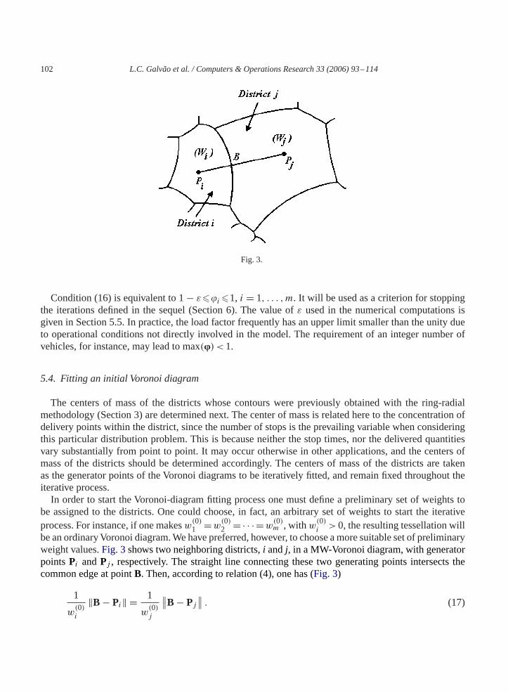
be an ordinary Voronoi diagram. We have preferred, however, to choose a more suitable set of preliminaryweight values.Fig. 3shows two neighboring districts,i andj, in a MW-Voronoi diagram, with generatorpointsPi andPj , respectively. The straight line connecting these two generating points intersects thecommon edge at pointB. Then, according to relation (4), one has (Fig. 3)

1

w(0)i

‖B− Pi‖ = 1

w(0)j

∥∥B− Pj

∥∥ . (17)


If we assimilate the districts to circles with equivalent areas, their radiiri andrj will be proportionalto the square roots of the areas. This suggests putting

‖B− Pi‖∥∥B− Pj

∥∥ �ri

rj�

√Ai√Aj

(18)

and, by combining Eqs. (17) and 18

w0i

w0j

�

√Ai√Aj

. (19)

Adopting a set of strictly positive weights respecting (19), the corresponding initial MW-Voronoidiagram is generated. Okabe et al.[21] point out that a MW-Voronoi region may not be connected,depending on the relative values of the weights. This situation may arise when the weights of adjacentdistricts are too discrepant. For the problem under analysis and the methodology proposed, such a situationmay arise if the continuous approximations of the density of servicing points, the quantities of deliveredcargo and the stopping times do not vary smoothly (large peaks or singularities). In this work, we have onlyconsidered situations where these quantities vary smoothly enough in order to avoid such irregularities.

5.5. The iterative fitting process

The objective is to get a MW-Voronoi diagram satisfying:

(a) the generator points are the centers of mass of the previously obtained wedge-shaped districts;(b) the criterion of homogeneous partition (15) is satisfied for a given value of the tolerance coefficient

ε >0.

Let us introduce a continuous function� : R → R such that

(i) �(x) = 1 if and only if 1− ��x�1,(ii ) �(x)>1 if and only if x <1 − �,

(iii ) �(x)<1 if and only if x >1,(iv) �min��(x)��max, 0< �min <1< �max. (20)

The values of�min and�max used in the calculations are given in Section 6.1.The iterative procedure works as follows:

• Step�=0: generation of the initial MW-Voronoi diagram and associated weightsw(0)=(w

(0)1 · · ·w(0)

m

)as described in Section 5.4.

• Step�>0: the weightsw(�−1) =(w

(�−1)1 . . . w

(�−1)m

)the load factors�(�−1) =

(�(�−1)

1 . . .�(�−1)m

)and their extrema�(�−1)

min nd�(�−1)max are known. If these last values satisfy condition (16), the iterations

stop: the MW-Voronoi diagram associated to the weightsw(�−1) gives a homogeneous partition.


If not, the weights are multiplied by the coefficients�(�) =(�(�)

1 . . . �(�)m

):

w(�)i = �(�)

i w(�−1)i , �(�)

i = �(�(�−1)

i

), i = 1, . . . , m. (21)

and we start the step� + 1.

5.6. Convergence of the MW-Voronoi diagram fitting process

We have the following result:Theorem. Assume that the sequence of weights

{w(�)

}��0 ⊂ Rm converges tow ∈ Rm, such that

w��>0 (i. e.,wi ��>0,i=1, . . . , m).Then, theclusterpointsof theprocesscorrespond tohomogeneouspartitions satisfying condition(16).

The inequalityw�� means that the iterative procedure does not generate empty Voronoi regions. Aviolation of this condition shows that the total number of vehiclesm is excessive and may be decreased.Proof of the theorem. Let us apply Eq. 21 recursively: we get

w(�)i =

�∏

j=1

�(j)i

w

(0)i . (22)

Thus

C(�)i =

�∏j=1

�(j)i = w

(�)i

w(0)i

−→�→∞

wi

w(0)i

>0. (23)

Consequently�(�) → � = (1, . . . ,1), i.e.,�(�)i −→

�→+∞ 1, for i = 1, . . . , m, since

�(�)i = C

(�)i /C

(�−1)i −→

�→∞wi/w

(0)i

wi/w(0)i

= 1. (24)

Moreover, the load factors are bounded independently of the partition: there is a constant�>0 such that0��(�)

min��(�)max��, for any��0 (� may be interpreted as the load factor if a single vehicle is considered

instead ofm vehicles). Thus, the sequence{�(�)

}��0 ⊂ Rm is bounded and the Bolzano–Weierstrass

theorem yields the existence of cluster points: for a subsequence,�(�) → �=(�1, . . . ,�m).The continuityof the function� shows that�i = �(�i). Since�i = 1, we have 1− ��i �1 and any cluster point verifies(16).

5.7. Effect on total distribution cost

Although the Voronoi-diagram partitioning process changes the shape of the districts, also changingtheir orientation in a minor scale, it can be shown that this particular smoothing technique does notseriously affect the resulting total distribution cost. The optimal cost per demand point consists of threecomponents: first, the per stop cost; second, the average local traveling cost, which depends on the distancetraveled in the zone; and third, the line-haul cost, which depends on the distance from the district to the


depot[11,12,16]. There are cases where some costs are better expressed as being proportional to traveltime, typically when the driver’s wage is the predominant element[12]. For such cases one can simplyconvert travel distance into travel time by applying the corresponding average speed.

Since the type of vehicle is not changed when running the preliminary wedge-shaped version andsubsequently the MW-Voronoi diagram model, and since demand characteristics remain unchanged, thetotal handling cost (delivering cargo at the customers’ places) does not change as well.

Next, in order to analyze the two other cost components, and following Newell and Daganzo[12],the line-haul distance and the local traveled distance are treated in a slightly different way. Although theactual line-haul travel to a district is usually measured to or from points of the zone with the shortest traveldistance from the depot, that is the near end of the zone, Newell and Daganzo[12,13]defined theline-haultravelas the distance from the source to the center of the district, so that the total line-haul distance in theregion would be independent of the orientation of the zones. Thus, the total line-haul distance is twice thesum of the Euclidean radial distances from the depot (corrected by a route factor) to all district centers.This is independent of any strategy for local delivery[13]. Since the district centers remain unchangedwhen running the preliminary ring-radial version and the MW-Voronoi diagram model, one concludesthat the total line-haul cost does not change as well.

The local travel distance, on its turn, is determined from (6), less the saving in line-haul distancebetween the end of the zone and its center[13]. First, expression (6) presupposes that the points areuniformly and independently scattered over the area and the district is fairly compact and convex. It canbe applied to most metrics, giving reasonable results forn>15, and holding quite well for different districtshapes[33,30,34]. These conditions are all observed in the present application. Therefore, two equivalentdistricts, one obtained with the ring-radial model and the other with the Voronoi diagram approach, bothwith the same areaA and equal number of servicing pointsn, will approximately show the same localtravel distance, except for the saving in line-haul distance between the end of the zone and its center.

Second, departing from (6), one can show that the average local traveled distance between successivedelivery points is proportional to�−1/2 [13]. Since, by hypothesis, the density of servicing points isnearly constant over distances comparable with a district size, and the total number of demand points inthe regionR is constant, one concludes that slight variations ofA andn between adjacent districts willnot appreciably change the total local distance for the entire region.

Third, the larger the region (that is the larger the number of zones), the larger is the line-haul distance ascompared with the local travel distance[13]. As pointed out by Newell and Daganzo[13], any fractionalerror in the local distance from its minimum, due to different savings in line-haul distance betweenthe end of the zone and its center, will contribute a much smaller fractional error in the total traveldistance (a negligible error for a sufficiently large region). Therefore, slight variations of the shape of thedistricts and on its orientation will not significantly affect the total local traveled distance for the entireregion. In addition, Newell and Daganzo[12] state that the total distribution cost is insensitive to thedesign parameters if they are chosen to be close to their optimal values, so one need not determine themvery accurately. Thus, given the level of accuracy obtained with continuous approximations, an eventualfractional error in the local distance from its minimum will not significantly affect the total distributioncost.

The conclusion is that the smoothing process with weighted Voronoi diagrams is sub-optimal, but theeffect on the total distribution cost tends to be small enough. Actually, diverse sub-optimal distributionstrategies are encountered in the literature[11–15,20,30]. The adoption of a near optimal strategy is oftenexplained by the need of getting more intuitive tours or by another simplifying objective.


6. Computational considerations

6.1. Numerical considerations about the choice of the function�

The choice of� has a wide numerical influence: for instance, if (�min, �max) corresponds to a too largeinterval, a large dispersion of the weights may be generated along the iterations and the resulting MW-Voronoi diagram may contain unconnected districts. In order to avoid such an undesirable disconnection,the choice of the function� must lead to small weight improvements at each stage of the computation.

We use in this work a particular choice of� which has shown to satisfy this condition: we set�(x) =�(�(x)), where� is the piecewise linear function such that

�(x) = �max(1 − �) − �min

(1 − �) − �min+ 1 − �max

(1 − �) − �minx if �min�x�1 − �,

�(x) = 1 if 1 − ��x�1,

�(x) = �min − �max

1 − �max+ 1 − �min

1 − �maxx if 1�x��max (25)

and� : R → R is the projection onto the interval (�min, �max), where 0< �min <1< �max are pre-definedconstants, and where� is given by

�(x) = �min if x��min,

�(x) = x if �min�x��max,

�(x) = �max if x��max. (26)

With this choice, we have�(�)i =�

(�(�−1)i

), �(�−1)

i =�(�(�−1)

i

), and�(�−1)

i will be truncated whenever

its value is greater than�maxor smaller than�min, what reduces the variation of the corresponding weightsduring the iterations. The truncation is only intended to furnish a better numerical behavior, having noother physical or operational meaning.

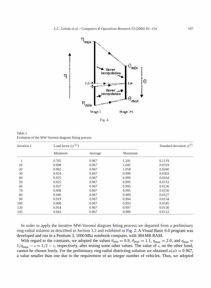
Since the values of�i are destined to lie in the interval 1− � ��i �1 at the end of the process, weadopted�min= (1/�max)− �. This choice can be explained with the help ofFig. 4. There is an indifferenceinterval 1− ��(�−1)

i �1 for which �(�)i is equal to the unit. Thus, in order to maintain a correcting

interval of size 1/�max for �(�−1)i �1 − �, we set�min = (1/�max) − � (seeFig. 4). Of course, one must

have��(1/�max) in order to get non-negative values for�(�−1)i . We take also�max= 2− �min in order to

distribute the possible values of�(�)i on the interval having center 1 (cf.Fig. 4).

6.2. Results

The described methodology was applied to the example analyzed in[16], extracted from a parceldelivery case in the city of São Paulo, Brazil. The metropolitan regionR served by the distributionservice has an area of 666 km2 and is inscribed in a rectangle of sides 30.135× 34.300 km (Fig. 1). Theregion was divided into elementary square cells of 35 m side. Other elementary cell dimensions wereanalyzed, varying from 35 m to about 200 m. Although the adoption of larger elementary cells will reducethe computation time, a raster structure with elementary cells of 35-meter side was a good compromisewhen confronting computation time and accuracy.


Fig. 4.

Table 1Evolution of the MW-Voronoi diagram fitting process

Iteration� Load factor (�(�)) Standard deviation�(�)

Minimum Average Maximum

1 0.765 0.967 1.241 0.111910 0.898 0.967 1.045 0.031920 0.902 0.967 1.058 0.024030 0.924 0.967 0.999 0.020340 0.925 0.967 0.999 0.016450 0.925 0.967 0.995 0.015360 0.937 0.967 0.995 0.013670 0.908 0.967 0.995 0.015680 0.940 0.967 0.989 0.012790 0.919 0.967 0.994 0.0134

100 0.908 0.967 0.993 0.0145120 0.934 0.967 0.997 0.0130145 0.943 0.967 0.989 0.0112

In order to apply the iterative MW-Voronoi diagram fitting process we departed from a preliminaryring-radial solution as described in Section 3.2 and exhibited inFig. 2. A Visual Basic 6.0 program wasdeveloped and run in a Pentium 3, 1000 Mhz notebook computer, with 384 MB RAM.

With regard to the constants, we adopted the values�min = 0.9, �max = 1.1, �max = 2.0, and�min =1/�max − � = 1/2 − �, respectively, after testing some other values. The value of�, on the other hand,cannot be chosen freely. For the preliminary ring-radial districting solution we obtaineda(�) = 0.967,a value smaller than one due to the requirement of an integer number of vehicles. Thus, we adopted


Fig. 5.

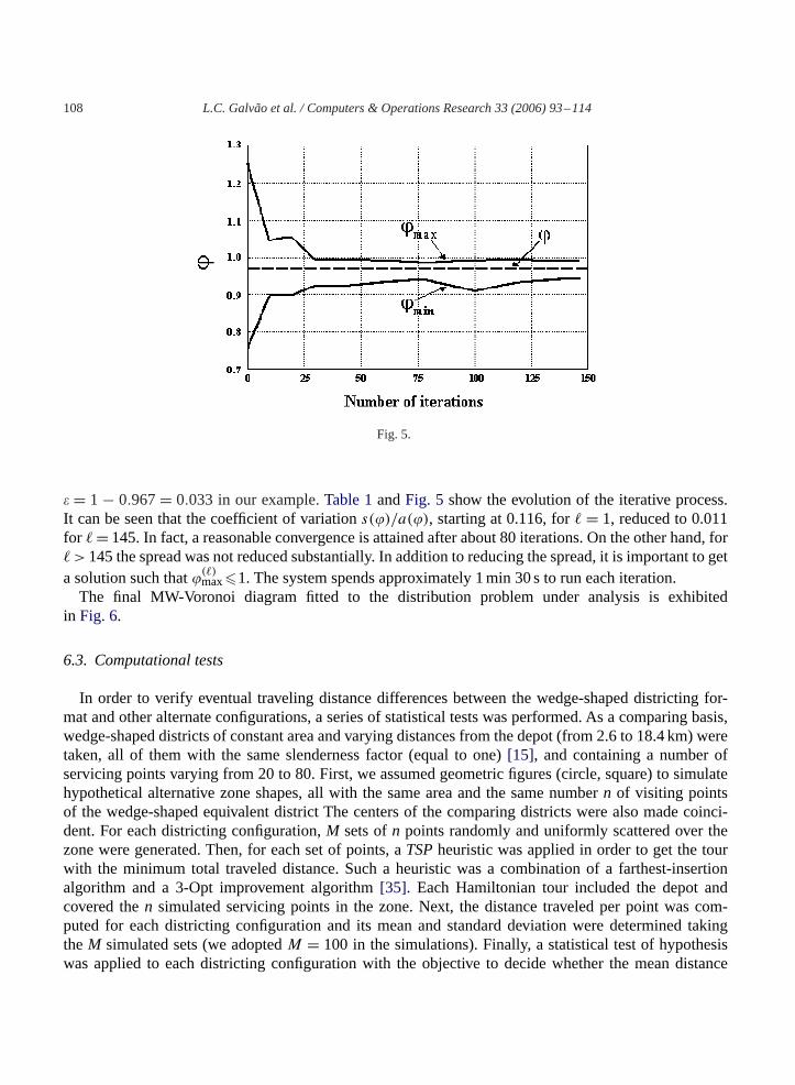
� = 1 − 0.967= 0.033 in our example.Table 1andFig. 5 show the evolution of the iterative process.It can be seen that the coefficient of variations(�)/a(�), starting at 0.116, for� = 1, reduced to 0.011for � = 145. In fact, a reasonable convergence is attained after about 80 iterations. On the other hand, for�>145 the spread was not reduced substantially. In addition to reducing the spread, it is important to geta solution such that�(�)

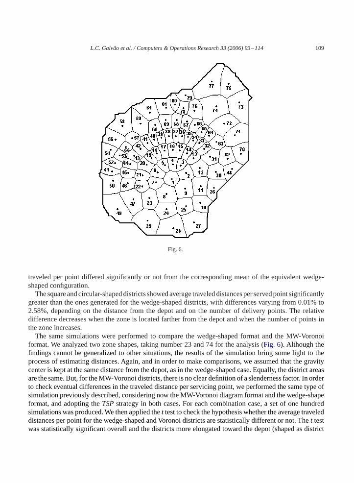
max�1. The system spends approximately 1 min 30 s to run each iteration.The final MW-Voronoi diagram fitted to the distribution problem under analysis is exhibited

in Fig. 6.

6.3. Computational tests

In order to verify eventual traveling distance differences between the wedge-shaped districting for-mat and other alternate configurations, a series of statistical tests was performed. As a comparing basis,wedge-shaped districts of constant area and varying distances from the depot (from 2.6 to 18.4 km) weretaken, all of them with the same slenderness factor (equal to one)[15], and containing a number ofservicing points varying from 20 to 80. First, we assumed geometric figures (circle, square) to simulatehypothetical alternative zone shapes, all with the same area and the same numbern of visiting pointsof the wedge-shaped equivalent district The centers of the comparing districts were also made coinci-dent. For each districting configuration,M sets ofn points randomly and uniformly scattered over thezone were generated. Then, for each set of points, aTSPheuristic was applied in order to get the tourwith the minimum total traveled distance. Such a heuristic was a combination of a farthest-insertionalgorithm and a 3-Opt improvement algorithm[35]. Each Hamiltonian tour included the depot andcovered then simulated servicing points in the zone. Next, the distance traveled per point was com-puted for each districting configuration and its mean and standard deviation were determined takingtheM simulated sets (we adoptedM = 100 in the simulations). Finally, a statistical test of hypothesiswas applied to each districting configuration with the objective to decide whether the mean distance


Fig. 6.

traveled per point differed significantly or not from the corresponding mean of the equivalent wedge-shaped configuration.

The square and circular-shaped districts showed average traveled distances per served point significantlygreater than the ones generated for the wedge-shaped districts, with differences varying from 0.01% to2.58%, depending on the distance from the depot and on the number of delivery points. The relativedifference decreases when the zone is located farther from the depot and when the number of points inthe zone increases.

The same simulations were performed to compare the wedge-shaped format and the MW-Voronoiformat. We analyzed two zone shapes, taking number 23 and 74 for the analysis (Fig. 6). Although thefindings cannot be generalized to other situations, the results of the simulation bring some light to theprocess of estimating distances. Again, and in order to make comparisons, we assumed that the gravitycenter is kept at the same distance from the depot, as in the wedge-shaped case. Equally, the district areasare the same. But, for the MW-Voronoi districts, there is no clear definition of a slenderness factor. In orderto check eventual differences in the traveled distance per servicing point, we performed the same type ofsimulation previously described, considering now the MW-Voronoi diagram format and the wedge-shapeformat, and adopting theTSPstrategy in both cases. For each combination case, a set of one hundredsimulations was produced. We then applied thet test to check the hypothesis whether the average traveleddistances per point for the wedge-shaped and Voronoi districts are statistically different or not. Thet testwas statistically significant overall and the districts more elongated toward the depot (shaped as district


no 74) showed average traveled distances per point smaller than the equivalent wedge-shaped districts.On the other hand, the less elongated districts (shaped as district no 23) presented opposite results,with average traveled distances per point greater than the equivalent wedge-shaped districts. Absolutedifferences varied from 0.6% to 3.1%, depending on the distance from the depot and on the number ofdelivery points.

In general, the more elongated is the district toward the depot, the shorter will be the link between thedepot and the first and the last points of theTSPtour within the zone. This introduces a double savingin the traveled distance. As a consequence, the average traveled distance tends to decrease as the zonebecomes more elongated toward the source. TakingVoronoi-diagram districts not too elongated toward thedepot, on the other hand, the trend is to obtain opposite results, i.e. the MW-Voronoi shaped districts mayyield average travel distances larger than the ones observable for the wedge-shaped district. In addition,when the distance of the district center from the depot increases, the average traveled distance per pointtends to comparatively decrease. This happens because any fractional error in the local distance from itsminimum, will contribute a much smaller fractional error in the total travel distance when the distancefrom the depot increases[12].

The average traveled distance per visited point was then computed for the whole served region, consid-ering the wedge-shaped format (Fig. 2) and the MW-Voronoi districting format (Fig. 6). The differencebetween both schemes was only 0.26%. Our findings have shown that, although the MW-Voronoi diagramdistricting approach introduces a penalty in the traveled distance or cost, the increment is small, providedthe districts are kept fairly convex and fairly compact, as stated in[33]. The varying shape, elongation,distance from the depot, and number of servicing points in the zones are balancing factors that make thefinal absolute difference relatively small.

7. Conclusions

We have presented a method to solve a logistics districting problem with the aid of a MW-Voronoidiagram fitting process. The method was applied to solve a parcel delivery problem in the city of SãoPaulo, Brazil, which was previously analyzed in[16]. The resulting district contours, as depicted inFig.6, are smoothed and closer to the configuration contours encountered in practical situations. The resultingrepartition of the region led to more balanced time/capacity utilization (load factors) across the districts.Considering the coarse underlying road-network approximation (Euclidean metric associated with a routefactor), and the fact that a small error in the parameters tend to give only a much smaller increase in thecost [12], we conclude that the MW-Voronoi diagram fitting process is a valid methodology to solvepractical distribution districting problems.

Apart from obtaining smoothed district partitions, the utilization of Voronoi diagrams opens the pos-sibility for further exploring some of its properties in order to get better approximations to real-worldproblems. In special, Voronoi diagrams allow for the introduction of physical obstacles into the model[21,25]. This kind of situation occurs frequently in urban distribution problems, with obstacles imposedby thoroughfares, highways, rivers, reservoirs, hills, etc. We are presently extending our research as toincorporate obstacles in the districting process. Furthermore, improvements in the numerical process mayalso be obtained by considering other expressions for the function�, or other weight forms, differentlyfrom Eq. 21.


Acknowledgements

This research was partially supported by the National Council for Scientific and Technological Devel-opment (CNPq), Brazil, projects 520474/96-1 and 500031/02-9.

Appendix A.

In this appendix, we describe the continuous approximation technique that was used in the paper.

7.1. Demand level representation

Let us consider a regionR containing a setSformed byn servicing points

S = {Si = (xi, yi), i = 1, . . . , n} ⊂ R. (A.1)

For each(x, y) ∈ R2 we define

S(x, y) = {Si ∈ S |xi �x and yi �y} . (A.2)

Let U be a quantity associated to the servicing points. For instance, when computing the number ofpoints

U(S) = 1 if S= (x, y) ∈ S, U(S) = 0 otherwise. (A.3)

We introduce a bi-dimensional cumulative functionF: R2 → R such that

F(x, y) =∑

Si∈S(x,y)

U(Si). (A.4)

Considering Eq. (A.3),U represents the number of servicing points having the coordinates limited bythe upper bounds(x, y):

F(x, y) = cardS(x, y). (A.5)

In the framework of statistical description of data, a cumulative functionFp is usually introducedand gives the relative frequency (probability) ofS(x, y). F is analogous toFp, except that it gives theabsolute number of servicing points and not a frequency or a probability.Fp andF are connected bythe simple relationF = nFp, and have analogous properties: namely, a densityf may be associated toF, analogous to the density of probabilityfp associated toFp. Since the setS is discrete, functionF isdiscontinuous andf is a sum of Dirac measures. In the sequel, we shall introduce a regular approximationF of the functionFhaving suitable mathematical properties of differentiability. Namely, the approximateddensityf associated to the approximationF , given by

f (x, y) = �2F (x, y)/�x �y, (A.6)

will be a continuous function. This procedure is analogous to the construction of regular approximationsFp andfp of Fp andfp, respectively. For a given subsetA ⊂ R, the value ofU associated toA is given


by the sum of the values ofU for the servicing points ofA:

U(A) =∑Si∈A

U(Si) =∫A

f (x, y)dx dy. (A.7)

We approximate

U(A) ≈ F (A) =∫A

f (x, y)dx dy. (A.8)

In the application analyzed in this paper, the variablef (x, y) may represent: (a) the existence of apoint at(x, y), (b) the quantity of product delivered at point (x, y), and (c) the stopping time to servicethat point.

Methods for the construction of the regular approximationsF and f may be found in the literature.In this work, we shall use an approximation by splines combined with a finite element discretization ofthe regionR. Our choice is guided by our final objective: the optimization procedures imply repeatedevaluations of the quantities defined by Eq. (A.8).

7.2. Spline approximation and finite element discretization

A convenient way to reduce the computational effort is the discretization of the regionR by using afinite element mesh: the nodal values off or F may be computed prior to the optimization and stored asa table of values. These values are used to evaluate Eq. (A.8) on each element. For instance, letE be afinite element havingp nodesN1, . . . ,Np. We notefi = f (Ni) andf = (f1, . . . , fp)

T. On the elementE, F is a function of the nodal values

F (x, y) =∑

i=1,...,k

ai(f )�i(x, y). (A.9)

Functions�i , i=1, . . . , k, are shape functions associated to the finite approximation and�=(�1, . . . , �k)T

is the local basis of approximation, anda= (a1, . . . , ak)T are the local coefficients of the approximation.

Both� anda vary withE. One has

F (E) =∑

i=1,...,k

iai(f ); i =∫A

�i(x, y)dx dy. (A.10)

Shape functions are chosen according to the desired regularity of the approximationf. For the standardfinite element approximation methods,a is a linear function off , i.e.,a=Mf , whereM is ak×p matrix.In this case,F (E) is a weighted sum of the values off at each node

F (E) = zTf , z=MT�, (A.11)

wherez=(z1, . . . , zp)T and�=(, . . . ,k)

T.As previously observed, all these values may be computedprior to the optimization procedure. They are used with the latter in order to compute the value ofF (A)


for an arbitraryA, by adding the contributions of the elements forming A (eventually a correction isintroduced for the elements lying only partially inA):

F (A) =∑

Ei∩A =

F (Ei). (A.12)

An useful situation adopted in this paper is to consider quadrilateral finite elements with four nodes(Q1 finite elements), which each elementE is a rectangleRABCD with verticesA = (xmin, ymin), B =(xmin, ymax), C = (xmax, ymax) andD = (xmax, ymin), the nodes being the vertices. For this case

F (E) = F (C) − F (B) − F (D) + F (A). (A.13)

Due to the simplicity of Eq. (A.13), the use ofQ1 finite elements saves computational time, and thus itis used in our calculations, but actually the method may be implemented with any kind of finite elementmesh, by using the appropriate weightszi and Eq. (A.9) in order to evaluateF(E). In this work we considerthat the expression (A.9) is evaluated by using linear functions onto each element, corresponding to thelocal basis

� = 〈1, x − xmax, y − ymax〉. (A.14)

This means an approximationF of F by a bi-quadratic spline, corresponding to the local basis� = 〈1,x − xmax, y − ymax, (x − xmax)(y − ymax), (x − xmax)

2, (y − ymax)2〉, according to Eq. (A.6).

References

[1] Bozkaya B, Erkut E, Laporte G. A tabu search heuristic and adaptive memory procedure for political districting. EuropeanJournal of Operational Research 2003;144:12–26.

[2] Mehrotra A, Johnson EL, Nemhauser GL. An optimization based heuristic for political districting. Management Science1998;44(8):1100–14.

[3] Williams Jr JC. Political redistricting: a review. Papers in Regional Science 1995;74:13–40.[4] Guo J, Trinidad G, Smith N. Mozart: a multi-objective zoning and aggregation tool. Proceedings of the Philippine

Computing Science Congress, 2001, p. 197–201.[5] Hojati M. Optimal political districting. Computers and Operations Research 1996;23(12):1147–61.[6] Schoepfle OB, Church RL. A new network representation of a “classic” school districting problem. Socio-Economic

Planning Science 1991;25(3):189–97.[7] D’Amico SJ, Wang SJ, Batta R, Rump CM. A simulated annealing approach to police district design. Computers and

Operations Research 2002;29(6):667–84.[8] Boots B, South R. Modeling retail trade areas using higher-order, multiplicatively weighted Voronoi diagrams. Journal of

Retailing 1997;73(4):519–36.[9] Muyldermans L, Cattrysse D, Van Oudheusden D, Lotan T. Districting for salt spreading operations. European Journal of

Operational Research 2002;3(139):521–32.[10] Zhou G, Min H, Gen M. The balanced allocation of customers to multiple distribution centers in the supply chain network:

a genetic algorithm approach. Computers and Industrial Engineering 2002;43:251–61.[11] Han AFW, Daganzo CF, Distributing nonstorable items without transshipments. Transportation Research Record, TRB,

Washington, DC 1996; (1061): 32–41.[12] Newell GF, Daganzo CF. Design of multiple-vehicle delivery tours—I a ring-radial network. Transportation Research B

1986;20B(5):345–63.[13] Newell GF, Daganzo CF. Design of multiple-vehicle delivery tours—II other metrics. Transportation Research B

1986;20B(5):365–76.


[14] LangevinA, Saint-MleuxY.A decision support system for physical distribution planning. Revue des Systémes de Décisions1992;1(2–3):273–86.

[15] Novaes AG, Graciolli OD. Designing multi-vehicle tours in a grid-cell format. European Journal of Operational Research1999;119:613–34.

[16] Novaes AG, Souza de Cursi JE, Graciolli OD. A continuous approach to the design of physical distribution systems.Computers and Operations Research 2000;27(9):877–93.

[17] Daganzo CF. Logistics systems analysis. Berlin: Springer; 1996.[18] LangevinA, Mbaraga P, Campbell JF. Continuous approximation models in freight distribution: an overview.Transportation

Research B 1996;30(3):163–88.[19] DasciA,VerterV.A continuous model for production-distribution system design. European Journal of Operational Research

2001;129:287–98.[20] Langevin A, Soumis F. Design of multiple-vehicle delivery tours satisfying time constraints. Transportation Research

1989;23B(2):123–38.[21] Okabe A, Boots B, Sugihara K. Spatial tessellations concepts and applications of Voronoi diagrams. Chichester: Wiley;

1995.[22] Okabe A, Suzuki A. Locational optimization problems solved through Voronoi diagrams. European Journal of Operational

Research 1997;98:445–56.[23] OkabeA, Boots B, Sugihara K. Nearest neighborhood operations with generalizedVoronoi diagrams: a review. International

Journal of Geographical Information System 1994;8(1):43–71.[24] Galvão LC. Dimensioning logistics distribution services with multiplicatively-weighted Voronoi diagrams (in Portuguese),

doctoral dissertation, Department of Industrial Engineering, Federal University of Santa Catarina, Florianópolis, SC, Brazil,2003.

[25] da Silva, ACL. Districting strategy in logistics problems using Voronoi diagrams with obstacles (in Portuguese), doctoraldissertation, Department of Industrial Engineering, Federal University of Santa, Catarina, Brazil, 2004.

[26] Boor C. A practical guide to splines. New York: Springer; 2001.[27] Spath H. Two dimensional spline interpolation algorithms. Wellesley, MA, USA: AK Peters Ltd.; 1995.[28] Zienkiewicz OC. The finite element method. London: McGraw-Hill; 1979.[29] Bathe K. Finite element procedures in engineering analysis. Englewood Cliffs, NJ, USA: Prentice-Hall; 1982.[30] Daganzo CF. The distance traveled to visitN points with a maximum ofC stops per vehicle: an analytic model and an

application. Transportation Science 1984;18:331–50.[31] Brimberg J, Love RF, Walker JH. The effect of axis rotation on distance estimation. European Journal of Operational

Research 1995;80:357–64.[32] Love RF, Morris JG, Wesolowsky GO. Facilities location: models and methods. New York: North-Holland; 1988.[33] Larson RC, Odoni AR. Urban operations research. Englewood Cliffs: Prentice-Hall; 1981.[34] Eilon S, Watson-Gandy CDT, Christofides N. Distribution management: mathematical modelling and practical analysis.

New York: Hafner; 1971.[35] Syslo MM, Deo N, Kowalik JS. Discrete optimization algorithms with Pascal programs. Englewood Cliffs: Prentice-Hall;

1983.

A multiplicatively-weighted Voronoi diagram approach to logistics districting

Documents