A multinomial logit approach to exchange rate policy classification with an application to growth q Justin M. Dubas a , Byung-Joo Lee b , Nelson C. Mark c, * a Texas Lutheran University, USA b University of Notre Dame, USA c University of Notre Dame and NBER, Economics & Economet, 442 Flanner, Notre Dame, IN 46556, USA JEL Classification: F3 F4 Keywords: Exchange rate regime de facto classification Growth abstract We model a country's de jure exchange rate policy as the choice from a multinomial logit response conditioned on the volatility of its bilateral exchange rate, the volatility of its international reserves, and the volatility of its effective exchange rate. The category with the highest predictive probability implied by the logit regressions serves as our de facto exchange rate policy. An empirical investigation into the relationship between the de facto classifications and GDP growth finds that growth is higher under stable currency-value policies. For non-industrialized countries, a more nuanced characterization of exchange rate policy finds that those who exhibit 'fear of floating' experience significantly higher growth. Ó 2010 Elsevier Ltd. All rights reserved. 1. Introduction Accurate, rigorous, and scientific classifications of exchange rate policy are an important ingre- dient for assessing the merits between fixed and floating exchange rates. Until relatively recently, empirical research employed the de jure classification, which largely reflects the self-reported policy submitted by a country's central bank to the International Monetary Fund. However, many observers q This paper was previously circulated under the title ``Effective Exchange Rate Classifications and Growth.'' We thank seminar participants at Notre Dame's Econ Brownbag workshop, the Kellogg Institute, and an NBER IFM program meeting for useful comments. * Corresponding author. E-mail address: [email protected] (N.C. Mark). Contents lists available at ScienceDirect Journal of International Money and Finance journal homepage: www.elsevier.com/locate/jimf 0261-5606/$ – see front matter Ó 2010 Elsevier Ltd. All rights reserved. doi:10.1016/j.jimonfin.2010.03.010 Journal of International Money and Finance 29 (2010) 1438–1462

Welcome message from author
This document is posted to help you gain knowledge. Please leave a comment to let me know what you think about it! Share it to your friends and learn new things together.
Transcript
Journal of International Money and Finance 29 (2010) 1438–1462
Contents lists available at ScienceDirect
Journal of International Moneyand Finance
journal homepage: www.elsevier .com/locate/ j imf
A multinomial logit approach to exchange rate policyclassification with an application to growthq
Justin M. Dubas a, Byung-Joo Lee b, Nelson C. Mark c,*
a Texas Lutheran University, USAbUniversity of Notre Dame, USAcUniversity of Notre Dame and NBER, Economics & Economet, 442 Flanner, Notre Dame, IN 46556, USA
JEL Classification:F3F4
Keywords:Exchange rate regimede facto classificationGrowth
q This paper was previously circulated under tseminar participants at Notre Dame's Econ Brownbuseful comments.* Corresponding author.
E-mail address: [email protected] (N.C. Mark).
0261-5606/$ – see front matter � 2010 Elsevier Ltdoi:10.1016/j.jimonfin.2010.03.010
a b s t r a c t
We model a country's de jure exchange rate policy as the choicefrom a multinomial logit response conditioned on the volatility ofits bilateral exchange rate, the volatility of its internationalreserves, and the volatility of its effective exchange rate. Thecategory with the highest predictive probability implied by thelogit regressions serves as our de facto exchange rate policy. Anempirical investigation into the relationship between the de factoclassifications and GDP growth finds that growth is higher understable currency-value policies. For non-industrialized countries,a more nuanced characterization of exchange rate policy finds thatthose who exhibit 'fear of floating' experience significantly highergrowth.
� 2010 Elsevier Ltd. All rights reserved.
1. Introduction
Accurate, rigorous, and scientific classifications of exchange rate policy are an important ingre-dient for assessing the merits between fixed and floating exchange rates. Until relatively recently,empirical research employed the de jure classification, which largely reflects the self-reported policysubmitted by a country's central bank to the International Monetary Fund. However, many observers
he title ``Effective Exchange Rate Classifications and Growth.'' We thankag workshop, the Kellogg Institute, and an NBER IFM program meeting for
d. All rights reserved.

J.M. Dubas et al. / Journal of International Money and Finance 29 (2010) 1438–1462 1439
have noted that the de facto currency management for some countries seemed at odds with their dejure management.1 As a result of such discrepancies, the de jure classification has been viewed asunsatisfactory for assessing the role of exchange rate stability in economic performance and hasmotivated researchers to propose de facto exchange rate classifications that are based on observedproperties of the foreign exchange market data. Influential contributions include the pioneeringwork of Reinhart and Rogoff (2004) (hereafter RR) and Levy-Yeyati and Sturzenegger (2003) (here-after LYS). RR argue that a natural classification of exchange rate policies should be based on thebehavior of the parallel market exchange rates on the grounds that they better reflect underlyingmarket and monetary conditions than do the country's official exchange rates whereas LYS advocatethe use of a k-means cluster algorithm to sort and assign countries to the various exchange ratepolicies.2
In this paper, we propose using a familiar econometric technique to obtain de facto classifications ofa nation's exchange rate policy. The procedure uses tools that are familiar to economists, producessensible results that are easily replicated, modified and updated. Specifically, we see three attractivefeatures in the approach. First, classifier judgment is required primarily in selecting the variables to beincluded in the exchange rate regime classificationmodel. Modifying and updating the classifications istherefore straightforward since one only needs to adjust the variables or update the data employed inestimation of the response problem. Second, the optimization criteria of our approach is familiar as it isbased on the likelihood principle and has well-known properties. Difficulties associated with 'incon-clusive' regimes often observed in RR and LYS methods are much less problematic. Third, it is feasiblewith our method to include a potentially large number of policy determinants.3
The idea that underlies our methodology goes like this. It must be the case that for many countries,the de jure exchange rate policy (regime) reported matches the de facto execution of that policy. Weassume that these de jure policies would seem to be thoughtful assessments of the degree of perceivedand economically relevant exchange rate stability experienced by that country. This is our motivationfor modeling the de jure classifications as the outcome of a multinomial logit response conditioned onmeasures of the volatility of the country's bilateral exchange rate against an anchor currency, thevolatility in the country's international reserves, and the volatility in the country's effective exchangerate. The unsystematic component–the error term in the model–captures unobservable factors thatcause some countries to deviate from the announced exchange rate policy. The classification that hasthe highest predictive probability implied by the model serves as the de facto policy. For ease ofreference, we refer to them as the LP (logit policy) classifications.
Two explanatory variables that we employ, the volatility of a bilateral nominal exchange rateagainst an anchor currency and the volatility of international reserves, follow directly from the liter-ature. This paper is the first to also use the volatility of the effective exchange rate. We give four reasons
1 Reference to potential inconsistencies between de jure and de facto regimes dates back at least to Frankel and Wei (1995While some de jure exchange rate fixers may appear to be de facto floaters due to frequent changes in their peg, others that arde jure floaters appear to be de facto fixers since they maintain very stable exchange rates – a phenomenon that Calvo anReinhart (2002) refer to as 'fear of floating.'
2 Assessing the role of a country's exchange rate regime in economic performance is an active area of research. The LYclassifications have been used by Juhn and Mauro (2002), who explore the long-run determinants of exchange rate regimeBordo and Flandreau (2001), who examine the link between financial depth and exchange rate regimes, Frankel et al. (2002who use it to examine the link between regime choice and local interest rate sensitivity, Edwards and Levy-Yeyati (2003) anBroda (2004), who analyze the impact of terms of trade on economic performance under different regimes. Both the LYS and Rregime classifications are used by Alesina and Wagner (2003) to find the politico-economic institutional qualities of countriewith different exchange rate regimes. RR is employed by Reinhart et al. (2003), who attempt to correlate the degree of exchangrate flexibility and degree and type of financial dollarization and Rogoff et al. (2004), who explore economic performance undealternative regimes.
3 Limiting the role of the classifier's judgment can be an advantage over RR's methodology: Because it is heavily dependenon their judgment, future research with their classifications may require RR to provide updates. The econometrics of ouapproach has some advantages over LYS's cluster analysis. LYS's method attempts to sort countries into exchange rate regimeby minimizing the unweighted average of within group sum of squared deviations from the group mean over each countrcharacteristic yielded 698 inconclusive country-year observations and is feasible only when the set of regime determinantssmall. Moreover, the optimality properties of their method are not well understood.
).ed
Ss,)dRser
trsyis
J.M. Dubas et al. / Journal of International Money and Finance 29 (2010) 1438–14621440
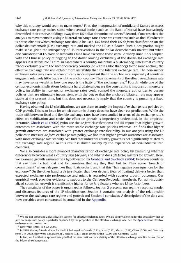
why this strategy would seem to make sense.4 First, the incorporation of multilateral factors to assessexchange rate policy makes sense when central banks (such as the Bank of Korea) have increasinglydiversified their reserve holdings away fromUS dollar denominated assets.5 Second, if one restricts theanalysis to movements in a single bilateral exchange rate, there are countries (such as the US) where itis not so obvious which exchange rate should be used. LYS based their US de facto classification on thedollar-deutschemark (DM) exchange rate and marked the US as a floater. Such a designation mightmake sense given the infrequency of US interventions in the dollar-deutschemark market, but whenone considers that US trade shares with China have exceeded those with Germany since 1995 coupledwith the Chinese policy of pegging to the dollar, looking exclusively at the dollar-DM exchange rateappears less defensible.6 Third, in cases where a country maintains a bilateral peg, unless that countrytrades exclusivelywith the anchor currency country (or within a bloc that pegs to the same anchor), theeffective exchange rate will exhibit more instability than the bilateral exchange rate. The non-anchorexchange rates may even be economically more important than the anchor rate, especially if countriesengage in relatively little tradewith the anchor country. Thusmovements of the effective exchange ratemay have some weight in how one reports the fixity of 'the exchange rate.'7 Fourth, while one of thecentral economic implications behind a hard bilateral peg are the constraints it imposes on monetarypolicy, instability in non-anchor exchange rates could compel the monetary authorities to pursuepolicies that are ultimately inconsistent with the peg so that the anchored bilateral rate may appearstable at the present time, but this does not necessarily imply that the country is pursuing a fixedexchange rate policy.
Having obtained the LP classifications, we use them to study the impact of exchange rate policies onGDP growth. This is an issue for which economic theory does not have clear-cut predictions. While thetrade-offs between fixed and flexible exchange rates have been studied in terms of the exchange rate'seffect on stabilization and trade, the effect on growth is imperfectly understood. In the empiricalliterature, Ghosh et al. (2002) (who use the de jure classifications) and RR report that higher growthoutcomes are associated with the more stable exchange rate policies whereas LYS finds that highergrowth outcomes are associated with greater exchange rate flexibility. In our analysis using the LPpolicies to measure de facto exchange rate policy, we find that higher growth outcomes are associatedwith more exchange rate stability. We find that industrial country growth is not significantly related tothe exchange rate regime so this result is driven mainly by the experience of non-industrializedcountries.
We also consider a more nuanced characterization of exchange rate policy by examining whetherdifferences betweenwhat a country says (de jure) and what it does (de facto)matters for growth. Here,we examine growth asymmetries hypothesized by Genberg and Swoboda (2004) between countriesthat say they fix but float and for countries that say they float but fix. They argue ``breach ofcommitment'' when a de jure fixer that floats de facto and that this ``has negative consequences for theeconomy.'' On the other hand, a de jure floater that fixes de facto (fear of floating) delivers better thanexpected exchange rate performance and might is rewarded with superior growth outcomes. Ourempirical work provides evidence to support to the Genberg-Swoboda hypothesis. For non-industri-alized countries, growth is significantly higher for de jure floaters who are LP de facto fixers.
The remainder of the paper is organized as follows. Section 2 presents our regime-response modeland discusses features of the LP classifications. Section 3 contains our analysis of the relationshipbetween the exchange rate regime and growth and Section 4 concludes. A description of the data andhow variables were constructed is contained in the Appendix.
4 We are not proposing a classification system for effective exchange rates. We are simply allowing for the possibility that dejure exchange rate policy is partially explained by the properties of the effective exchange rate. See the Appendix for effectiveexchange rate construction.
5 New York Times, Feb 22, 2005.6 In 1998, the top 5 trade shares for the U.S. belonged to Canada (0.21), Japan (0.12), Mexico (0.11), China (0.06), and Germany
(0.05). In 2002, they were Canada (0.21), Mexico (0.13), Japan (0.10), China (0.09), and Germany (0.05).7 In fact, we find that in approximately half of the observations the volatility of the effective exchange rate lies below that of
the bilateral exchange rate.
J.M. Dubas et al. / Journal of International Money and Finance 29 (2010) 1438–1462 1441
2. Classifying exchange rate policy
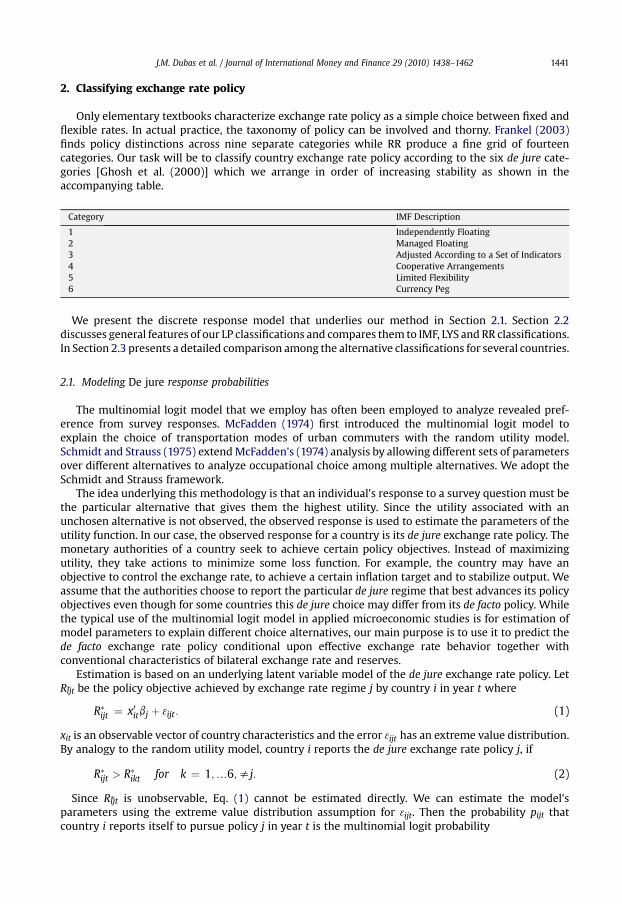
Only elementary textbooks characterize exchange rate policy as a simple choice between fixed andflexible rates. In actual practice, the taxonomy of policy can be involved and thorny. Frankel (2003)finds policy distinctions across nine separate categories while RR produce a fine grid of fourteencategories. Our task will be to classify country exchange rate policy according to the six de jure cate-gories [Ghosh et al. (2000)] which we arrange in order of increasing stability as shown in theaccompanying table.
Category IMF Description
1 Independently Floating2 Managed Floating3 Adjusted According to a Set of Indicators4 Cooperative Arrangements5 Limited Flexibility6 Currency Peg
We present the discrete response model that underlies our method in Section 2.1. Section 2.2discusses general features of our LP classifications and compares them to IMF, LYS and RR classifications.In Section 2.3 presents a detailed comparison among the alternative classifications for several countries.
2.1. Modeling De jure response probabilities
The multinomial logit model that we employ has often been employed to analyze revealed pref-erence from survey responses. McFadden (1974) first introduced the multinomial logit model toexplain the choice of transportation modes of urban commuters with the random utility model.Schmidt and Strauss (1975) extendMcFadden's (1974) analysis by allowing different sets of parametersover different alternatives to analyze occupational choice among multiple alternatives. We adopt theSchmidt and Strauss framework.
The idea underlying this methodology is that an individual's response to a survey question must bethe particular alternative that gives them the highest utility. Since the utility associated with anunchosen alternative is not observed, the observed response is used to estimate the parameters of theutility function. In our case, the observed response for a country is its de jure exchange rate policy. Themonetary authorities of a country seek to achieve certain policy objectives. Instead of maximizingutility, they take actions to minimize some loss function. For example, the country may have anobjective to control the exchange rate, to achieve a certain inflation target and to stabilize output. Weassume that the authorities choose to report the particular de jure regime that best advances its policyobjectives even though for some countries this de jure choice may differ from its de facto policy. Whilethe typical use of the multinomial logit model in applied microeconomic studies is for estimation ofmodel parameters to explain different choice alternatives, our main purpose is to use it to predict thede facto exchange rate policy conditional upon effective exchange rate behavior together withconventional characteristics of bilateral exchange rate and reserves.
Estimation is based on an underlying latent variable model of the de jure exchange rate policy. LetRijt* be the policy objective achieved by exchange rate regime j by country i in year t where
R�ijt ¼ x0itbj þ 3ijt : (1)
xit is an observable vector of country characteristics and the error 3ijt has an extreme value distribution.By analogy to the random utility model, country i reports the de jure exchange rate policy j, if
R�ijt > R�ikt for k ¼ 1;.6;sj: (2)
Since Rijt* is unobservable, Eq. (1) cannot be estimated directly. We can estimate the model'sparameters using the extreme value distribution assumption for 3ijt. Then the probability pijt thatcountry i reports itself to pursue policy j in year t is the multinomial logit probability

J.M. Dubas et al. / Journal of International Money and Finance 29 (2010) 1438–14621442
pijt ¼ exp x0itbjP � �; (3)
� �6K ¼1 exp x0itbk
where the coefficient vectorbjassociatedwithexchange rate regime j is estimatedwitha random-effectspanel regression.8 Country i declares de jure policy j because it is the choice that best achieves its policyobjective but not necessarily because it is the most accurate description of exchange rate behavior.
The regime categories in our multinomial logit specification are unordered. This has an importantadvantage over an ordered response model in our context because it allows for coefficient heteroge-neity across different policies. That is, for country i, we allow the impact of the characteristics on theresponse probability to differ across categories j ¼ 1,.6 whereas an ordered response model imposeshomogeneity restrictions on the coefficients across categories. We adopt the less restrictive approachsince our emphasis is on measurement as opposed to inference.
The country characteristics that we include in xit are
(i) the volatility of the effective exchange rate,(ii) the mean absolute change of the effective exchange rate,(iii) the volatility of the bilateral exchange rate relative to an anchor country,(iv) the mean absolute change of the bilateral exchange rate, and(v) the volatility of the country's international reserves.9
As with LYS and RR, we include reserve volatility because it is predicted to be directly related to the'fixity' in the exchange rate regime. The idea here is that high reserve volatility should be associatedwith frequent foreign exchange market intervention and active management. We also includemeasures of the volatility of the country's effective exchange rate which we constructed using tradeweights. Formany economies, the effective exchange ratemay convey relevant information concerningeconomic performance due to underlying exchange rate exposure that cannot be obtained froma single bilateral exchange rate.10
We then use the estimated model to predict the probability bpijt that a country with characteristicvector xit will pursue exchange rate policy j by assigning the country-year observation. We call thispredicted exchange rate regime the de facto regime. As there are a large number of coefficients toestimate and because the individual coefficient estimates do not have natural interpretations in thiscontext, we do not report them in the text but relegate them to the Appendix. The de facto exchangerate policy j for country i at time t is the policy with the highest predictive probability,
bpijt > bpijt for k ¼ 1;.6;sj (4)
We are also able to construct a continuous index of exchange rate policy using the predicted meanvalue
IDXit ¼X6k¼1
kbpikt : (5)
8 A normalization with respect to one of the regimes is required for identification. We use regime 5, which is the regime thatoccurs most frequently, for the normalization.
9 We use the same anchor countries as LYS to determine which bilateral exchange rate to use. We measure volatility as theannual sample standard deviation of the monthly percentage change in the respective variables. The mean absolute change foryear t is similarly computed from the annual average of monthly percentage changes. We note also that interest rate volatility isalso an important characteristic to determine exchange rate regimes. However, due to data availability, we lost a significantnumber of observations in estimation and we dropped the interest rate volatility from the estimation problem.10 Due to hyper-inflation countries, there are a non negligible number of outliers that we excluded by restricting the sample toobservations for the volatility of the nominal effective exchange rate to those less than 10% per annum. Doing so excluded theupper 4 percentile of observations. Similarly, we include only observations on the volatility of reserves that are less than 50%which excluded the upper 5 percentile of observations.

Table 1Logit exchange rate policy classifications.
LP LPB LPE
Frequency Percent Frequency Percent Frequency Percent
1 532 16.8 280 6.4 525 16.62 116 3.7 0 0 60 1.93 34 1.1 0 0 0 04 811 25.7 233 5.3 60 1.95 1602 50.7 3634 90.0 2445 77.46 64 2.0 234 5.3 70 2.2
Nobs 3159 3160 4381
Notes: LPB omits effective exchange rate volatility. LPE omits bilateral exchange rate volatility.
J.M. Dubas et al. / Journal of International Money and Finance 29 (2010) 1438–1462 1443
Since the de facto policy variable is discrete, this index can serve as a continuous proxy measure ofthe country's de facto exchange rate flexibility. We will use this index variable together with discreteexchange rate policy variable in the growth regressions in Section 3.
2.2. Properties of the LP classifications
Table 1 displays the distribution of the classifications generated by three alternative specifications ofthe country characteristics. Our preferred classification is listed under the LP heading and is generatedusing both measures of effective exchange rate dispersion (volatility and mean absolute deviation),the mean absolute change in the bilateral exchange rate and international reserve volatility.11
Including effective exchange rate volatility measures as a policy determinant is strongly supportedby the data as a likelihood ratio test for their exclusion yields a chi-square statistic of 165. With 10degrees of freedom, these 'zero-restrictions' are rejected at any reasonable level of significance.
It can be seen that most of the country-year observations are categorized as outcomes of relativelystable exchange rate policies falling in categories 4 (cooperative) and 5 (limited flexibility). Only 64observations are classified as hard fixers. The next largest classification is category 1 (independentlyfloating), which forms 17% of the observations.
What happens when only reserve volatility and bilateral exchange rate volatility are used? The clas-sification distribution obtained by dropping effective exchange rate volatility appears under the columnlabeled LPB (B for bilateral). Here, as with the de jure classifications, we see a substantial 'hollowing-out'of the intermediate ranges as we obtain no classifications in categories 2 or 3. This hollowing out issomewhat attenuated when the classifications are generated using only reserve and effective exchangerate volatility (labeled LPE). Here, we obtain nearly the same number of free-floaters, but many morefixers (categories 5 and 6). The point is that using only one measure of exchange rate volatility to theexclusion of the other results in a dearth of middle-range classifications. Because this seems to presenta distorted view of exchange rate policy, our preferred classification employs both measures.
Fig. 1 plots the evolution of the LP classifications along with the de jure, LYS, and RR classifications.12
Nearly all countries begin the sample as de jure fixers (categories 5 and 6). Then this proportiondeclines steadily over time. Increasingly, countries report themselves to pursue flexible exchange ratepolicies (categories 1 and 2).
The evolution of LP pure floaters is similar to that of de jure floaters. Very few country-yearobservations are classified as LP hard fixers. Most observations are placed in categories 1, 4, and 5 with
11 We originally performed estimation using all five variables but because bilateral exchange rate volatility and mean absolutechange measures are highly correlated (0.94) we dropped the volatility measure. Very similar results are obtained by keepingbilateral volatility and dropping the bilateral mean absolute change.12 Our LP classifications are not directly comparable to RR nor LYS since they do not provide a 6-way classification. For RR, wereversed and renumbered their 5-way classification broken down as 2) Freely falling, 3) Freely floating, 4) Managed floating, 5)Limited flexibility, 6) Peg. For LYS, we examine their 4-way classification broken down as 2) Flexible, 3) Dirty Float, 4) CrawlingPeg, and 5) Fixed. Both RR and LYS have a category for observations that are deemed 'inconclusive,' which we omitted indrawing the figures.

IMF (de jure) Logistic
0
0.1
0.2
0.3
0.4
0.5
0.6
0.7
0.8
0.9
1
1971 1974 1977 1980 1983 1986 1989 1992 1995 1998
1 2 3 4 5 6
0
0.1
0.2
0.3
0.4
0.5
0.6
0.7
0.8
0.9
1
1971 1975 1979 1983 1987 1991 1995 1999
1 2 3 4 5 6
LYS RR
0
0.1
0.2
0.3
0.4
0.5
0.6
0.7
0.8
0.9
1
1974 1977 1980 1983 1986 1989 1992 1995 1998
1 2 3 4
0
0.1
0.2
0.3
0.4
0.5
0.6
0.7
0.8
0.9
1
1971 1975 1979 1983 1987 1991 1995 1999
1 2 3 4 5
Fig. 1. Evolving distribution of alternative exchange rate policy classifications.
J.M. Dubas et al. / Journal of International Money and Finance 29 (2010) 1438–14621444
a relatively large proportion of category 5 policies (limited flexibility). There was a tendency to moveaway from fixing in the 1970s but the proportion of fixers has remained stable in the 1980s and 1990s.Interestingly, in comparing LP categories 5 and 6 to RR's category 5 and comparing LP categories 1 and2 to RR's categories 1 and 2, it can be seen that the LP classification exhibits a higher correspondence toRR's 'natural classification' than it does either to LYS or the de jure classifications. The distribution overtime of RR is relatively stable with many more intermediate policies than LP. One possible reason forthis stability is that RR employ a 5-year window for computing exchange rate variability whereas LPand LYS employed a one-year window. LYS consistently classifies the majority of observations into thefixed category. More than 70 percent of LYS observations were classified as fixers in 1974 andapproximately 55 percent were still fixers in 2000.
Table 2 shows the correlation matrix for the alternative classifications and the country character-istics that we used as determinants in producing the LP classification. Among alternative classifications,LP is most highly correlated with RR (0.53) and are least correlated with IMF de jure classifications(0.32). LP and RR (and LYS, barely) are negatively correlated with both measures of exchange ratevariability. Only de jure is not systematically related to volatility in the effective exchange rate.
LP is the classification that is most highly correlated with reserve volatility (although none areparticularly high), which indicates that more stablility in the exchange rate is associated with morereserve activity. 13 RR, on the other hand, is negatively correlated with reserve volatility which runscounter to the idea that reserves are used to stabilize the exchange rate.
13 Reserves can move around because the authorities are intervening in the foreign exchange market or for noninterventionactivities. We are unable to identify the underlying cause of these movements.
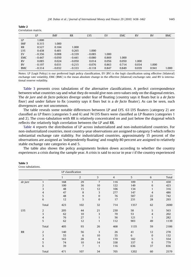
Table 2Correlation matrix.
LP IMF RR LYS EV EMC RV BV BMC
LP 1.000IMF 0.315 1.000RR 0.527 0.184 1.000LYS 0.438 0.401 0.265 1.000EV �0.356 0.008 �0.339 �0.085 1.000EMC �0.447 �0.050 �0.441 �0.080 0.869 1.000RV 0.085 0.024 �0.050 0.014 0.056 0.050 1.000BV �0.197 0.031 �0.215 �0.076 0.863 0.714 0.034 1.000BMC �0.314 �0.032 �0.333 �0.118 0.847 0.849 0.039 0.941 1.000
Notes: LP (Logit Policy) is our preferred logit policy classification, EV (BV) is the logit classification using effective (bilateral)exchange rate volatility, EMC (BMC) is the mean absolute change in the effective (bilateral) exchange rate, and RV is interna-tional reserve volatility.
J.M. Dubas et al. / Journal of International Money and Finance 29 (2010) 1438–1462 1445
Table 3 presents cross tabulations of the alternative classifications. A perfect correspondencebetweenwhat countries say andwhat they dowould give non-zero values only on the diagonal entries.The de jure and de facto policies diverge under fear of floating (country says it floats but is a de factofixer) and under failure to fix (country says it fixes but is a de facto floater). As can be seen, suchdivergences are not uncommon.
The table reveals some notable differences between LP and LYS. 63 LYS floaters (category 2) areclassified as LP fixers (categories 5 and 6) and 74 LYS fixers were classified as LP floaters (categories 1and 2). The cross-tabulation with RR is relatively concentrated on and just below the diagonal whichreflects the relatively high correlation between the LP and RR.
Table 4 reports the distribution of LP across industrialized and non-industrialized countries. Fornon-industrialized countries, most country-year observations are assigned to category 5 which reflectssubstantial exchange rate stability. For industrialized countries, approximately 15 percent of theobservations are assigned as 'independently floating' and roughly 80 percent are assigned to relativelystable exchange rate categories 4 and 5.
The table also shows the policy assignments broken down according to whether the countryexperiences a crisis during the sample year. A crisis is said to occur in year t if the country experienced
Table 3Cross tabulations.
LP classification
1 2 3 4 5 6 Total
de jure 1 168 29 7 116 109 1 4302 100 36 10 122 149 6 4233 48 15 12 106 134 1 3164 47 8 3 277 147 4 4865 48 9 0 76 587 22 7426 12 5 0 17 231 28 293
Total 423 102 32 714 1357 62 2690
LYS 2 205 44 21 230 58 5 5633 62 10 3 70 53 4 2024 76 27 1 56 121 1 2825 62 12 1 112 903 49 1139
Total 405 93 26 468 1135 59 2186
RR 2 140 56 3 26 41 12 2783 55 6 10 55 6 0 1324 163 28 6 170 182 5 5545 74 10 14 338 337 6 7796 39 7 1 116 636 37 836
Total 471 107 34 705 1202 60 2579

Table 4LP classifications across subgroups.
1 2 3 4 5 6 Total
Non-industrial (percent) 431 99 18 500 1361 63 2472(17) (4) (1) (20) (55) (3) 100
Industrial (percent) 101 17 16 311 241 1 687(15) (2) (2) (45) (35) (0) 100
Non-crisis (percent) 392 60 31 785 1561 52 2881(14) (2) (1) (27) (54) (2) 100
Crisis (percent) 140 56 3 26 41 12 278(50) (20) (1) (9) (15) (4) 100
J.M. Dubas et al. / Journal of International Money and Finance 29 (2010) 1438–14621446
a month-to-month change in its effective exchange rate exceeding 25 percent. Of 5760 country-yearobservations, therewere 434 crisis observations, 424 of which occurred in non-industrialized countriesand 10 for industrialized countries. Our methodology does not automatically assign crisis observationsto a free float since as can be seen, a relatively large share of crisis country-year observations continueto be grouped in categories 4 and above (28 percent).
2.3. Comparison of alternative de facto classifications for selected countries
In this section, we present several case studies of the alternative classifications.
Table 5Alternative classifications for selected emerging market economies.
Year Argentina Mexico Peru Korea
IMF LYS RR LP IMF LYS RR LP IMF LYS RR LP IMF LYS RR LP
1971 5 – 2 1 5 – 6 5 5 – – 5 5 – 4 11972 5 – 2 5 5 – 6 5 5 – – 5 5 – 4 51973 5 – 2 5 5 – 6 5 5 – – 5 5 – 4 51974 5 5 2 5 5 5 6 5 5 5 – 5 5 2 6 51975 5 3 2 1 5 5 6 5 5 2 – 5 5 4 6 51976 5 3 2 1 2 3 6 4 5 4 2 4 5 5 6 51977 5 2 2 1 2 2 6 5 3 4 2 1 5 5 6 51978 2 2 2 1 2 – 6 5 3 2 2 1 5 5 6 51979 3 2 5 1 2 – 6 5 2 2 2 2 5 5 6 51980 3 2 5 4 2 – 6 5 3 2 2 2 2 2 5 21981 3 3 2 1 2 4 5 4 3 2 2 2 2 4 5 51982 2 3 2 1 2 3 2 1 3 2 2 2 2 4 5 51983 2 4 2 2 2 4 2 2 1 4 2 2 2 5 5 41984 2 4 2 2 2 2 2 1 3 4 2 1 2 4 5 51985 2 3 6 1 2 4 2 1 5 4 2 1 2 3 5 51986 3 2 2 1 2 4 2 2 5 5 2 5 2 5 5 51987 2 4 2 1 2 4 2 1 5 4 2 1 2 5 5 51988 2 4 2 1 2 5 2 4 5 3 2 1 2 3 5 21989 2 – 2 1 2 3 5 4 5 3 2 2 2 5 5 51990 2 3 2 1 2 3 5 5 1 3 2 1 2 3 5 51991 6 3 6 2 2 5 5 5 1 4 2 1 2 5 5 51992 6 5 6 5 2 5 6 5 1 4 2 1 2 4 5 51993 6 5 6 1 2 5 6 5 1 2 2 1 2 4 5 51994 6 5 6 5 1 5 4 1 1 3 5 5 2 5 5 51995 6 5 6 5 1 3 2 2 1 2 5 1 2 3 5 41996 6 5 6 5 1 3 4 4 1 2 5 4 2 5 5 41997 6 5 6 5 1 2 4 1 1 4 5 5 1 4 5 11998 6 5 6 5 1 2 4 1 1 2 5 3 1 4 2 11999 6 5 6 5 1 2 4 1 1 2 6 4 1 5 3 12000 – 5 6 5 – 2 4 1 – – 6 5 – 5 3 42001 – – 6 5 – – 4 1 – – – 1 – – 3 42002 – – – 1 – – – 1 – – – – – – – 1
J.M. Dubas et al. / Journal of International Money and Finance 29 (2010) 1438–1462 1447
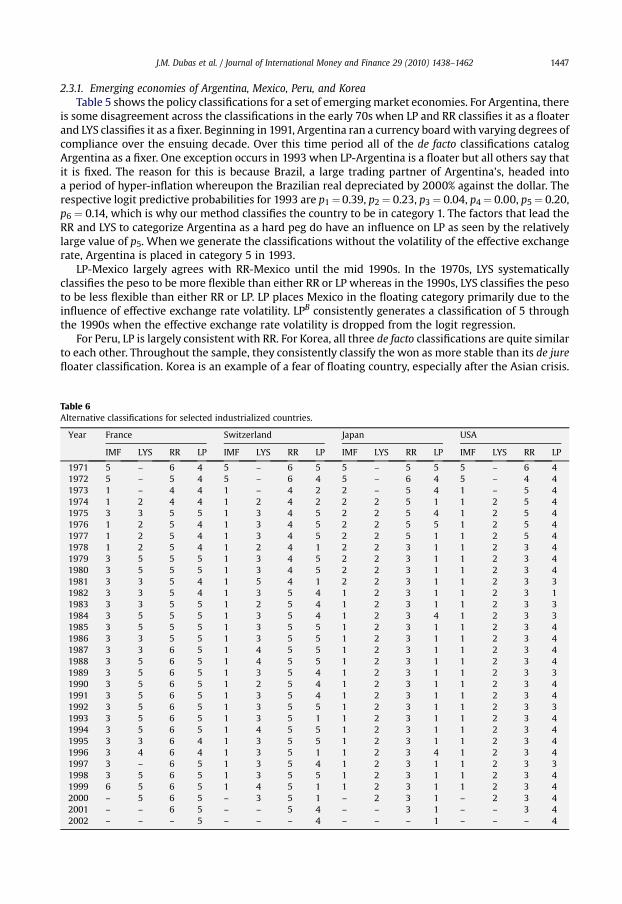
2.3.1. Emerging economies of Argentina, Mexico, Peru, and KoreaTable 5 shows the policy classifications for a set of emergingmarket economies. For Argentina, there
is some disagreement across the classifications in the early 70s when LP and RR classifies it as a floaterand LYS classifies it as a fixer. Beginning in 1991, Argentina ran a currency boardwith varying degrees ofcompliance over the ensuing decade. Over this time period all of the de facto classifications catalogArgentina as a fixer. One exception occurs in 1993 when LP-Argentina is a floater but all others say thatit is fixed. The reason for this is because Brazil, a large trading partner of Argentina's, headed intoa period of hyper-inflation whereupon the Brazilian real depreciated by 2000% against the dollar. Therespective logit predictive probabilities for 1993 are p1 ¼0.39, p2 ¼ 0.23, p3 ¼ 0.04, p4 ¼ 0.00, p5 ¼ 0.20,p6 ¼ 0.14, which is why our method classifies the country to be in category 1. The factors that lead theRR and LYS to categorize Argentina as a hard peg do have an influence on LP as seen by the relativelylarge value of p5. When we generate the classifications without the volatility of the effective exchangerate, Argentina is placed in category 5 in 1993.
LP-Mexico largely agrees with RR-Mexico until the mid 1990s. In the 1970s, LYS systematicallyclassifies the peso to be more flexible than either RR or LP whereas in the 1990s, LYS classifies the pesoto be less flexible than either RR or LP. LP places Mexico in the floating category primarily due to theinfluence of effective exchange rate volatility. LPB consistently generates a classification of 5 throughthe 1990s when the effective exchange rate volatility is dropped from the logit regression.
For Peru, LP is largely consistent with RR. For Korea, all three de facto classifications are quite similarto each other. Throughout the sample, they consistently classify the won as more stable than its de jurefloater classification. Korea is an example of a fear of floating country, especially after the Asian crisis.
Table 6Alternative classifications for selected industrialized countries.
Year France Switzerland Japan USA
IMF LYS RR LP IMF LYS RR LP IMF LYS RR LP IMF LYS RR LP
1971 5 – 6 4 5 – 6 5 5 – 5 5 5 – 6 41972 5 – 5 4 5 – 6 4 5 – 6 4 5 – 4 41973 1 – 4 4 1 – 4 2 2 – 5 4 1 – 5 41974 1 2 4 4 1 2 4 2 2 2 5 1 1 2 5 41975 3 3 5 5 1 3 4 5 2 2 5 4 1 2 5 41976 1 2 5 4 1 3 4 5 2 2 5 5 1 2 5 41977 1 2 5 4 1 3 4 5 2 2 5 1 1 2 5 41978 1 2 5 4 1 2 4 1 2 2 3 1 1 2 3 41979 3 5 5 5 1 3 4 5 2 2 3 1 1 2 3 41980 3 5 5 5 1 3 4 5 2 2 3 1 1 2 3 41981 3 3 5 4 1 5 4 1 2 2 3 1 1 2 3 31982 3 3 5 4 1 3 5 4 1 2 3 1 1 2 3 11983 3 3 5 5 1 2 5 4 1 2 3 1 1 2 3 31984 3 5 5 5 1 3 5 4 1 2 3 4 1 2 3 31985 3 5 5 5 1 3 5 5 1 2 3 1 1 2 3 41986 3 3 5 5 1 3 5 5 1 2 3 1 1 2 3 41987 3 3 6 5 1 4 5 5 1 2 3 1 1 2 3 41988 3 5 6 5 1 4 5 5 1 2 3 1 1 2 3 41989 3 5 6 5 1 3 5 4 1 2 3 1 1 2 3 31990 3 5 6 5 1 2 5 4 1 2 3 1 1 2 3 41991 3 5 6 5 1 3 5 4 1 2 3 1 1 2 3 41992 3 5 6 5 1 3 5 5 1 2 3 1 1 2 3 31993 3 5 6 5 1 3 5 1 1 2 3 1 1 2 3 41994 3 5 6 5 1 4 5 5 1 2 3 1 1 2 3 41995 3 3 6 4 1 3 5 5 1 2 3 1 1 2 3 41996 3 4 6 4 1 3 5 1 1 2 3 4 1 2 3 41997 3 – 6 5 1 3 5 4 1 2 3 1 1 2 3 31998 3 5 6 5 1 3 5 5 1 2 3 1 1 2 3 41999 6 5 6 5 1 4 5 1 1 2 3 1 1 2 3 42000 – 5 6 5 – 3 5 1 – 2 3 1 – 2 3 42001 – – 6 5 – – 5 4 – – 3 1 – – 3 42002 – – – 5 – – – 4 – – – 1 – – – 4

J.M. Dubas et al. / Journal of International Money and Finance 29 (2010) 1438–14621448
All of the de facto policies exhibit periods of volatility. The RR-Argentina jumps from 2 to 6 back to 2between 1984 and 1986. LYS-Peru jumps from 5 to 2 to 4 between 1974 and 1976 while LP-Peruswitches from 5 to 1 and back to 5 between 1992 and 1994. While LP tends to exhibit this sort ofvolatility when the estimated probabilities across classifications are relatively flat, the continuouspolicy index IDX is markedly less volatile and shows fewer extreme values.
2.3.2. High income and industrialized: US, France, Japan, and SwitzerlandThe results for these countries are shown in Table 6. LP-US places the dollar in an intermediate
regime and classifies it to be more stable than RR or LYS. The LP-France corresponds closely to RR byassessing the franc to be a relatively stable currency whereas LYS often classifies the franc to berelatively flexible. LP-Switzerland corresponds more closely to LYS than it does to RR which is sort ofunusual, and all of the de factomethods classify this country's exchange rate as more stable than its dejure classification. Notice that from 1973 onwards, Switzerland is a fear of floating country. LP-Japan islargely in agreement with RR and its de jure classification as a floater whereas LYS-Japan tends toclassify policy as being more stable.
De jure hard pegs classified as de facto fixes. Table 7 displays the classifications for Panama, Estoniaand St. Lucia. These are three countries for which a hard peg classification would seem to be incon-trovertible. These are Panama, which has dollarized, Estonia, which has a currency board, and St. Lucia,which has maintained a long-term stable peg. The three de facto methods generate similar results.
LP occasionally classifies Panama as a currency peg (category 6 in 1983 and 1984) but generally givesa classification of 5 on account of relatively low reserve volatility (which exceeds the cross-sectional
Table 7Alternative classifications for selected 'hard pegged' countries.
Year Panama Estonia St. Lucia
IMF LYS RR LP LPB IMF LYS RR LP LPB IMF LYS RR LP LPB
1971 5 – 6 5 5 – – – – – 6 – 6 – –
1972 5 – 6 5 5 – – – – – 6 – 6 – –
1973 6 – 6 5 5 – – – – – 6 – 6 – –
1974 6 5 6 5 5 – – – – – 6 5 6 – –
1975 6 5 6 5 5 – – – – – 6 5 6 – –
1976 6 5 6 5 6 – – – – – 6 5 6 – –
1977 6 5 6 5 6 – – – – – 6 5 6 – –
1978 6 5 6 5 5 – – – – – 6 5 6 – –
1979 6 5 6 5 5 – – – – – 6 5 6 – 51980 6 5 6 5 6 – – – – – 6 5 6 – 51981 6 5 6 5 5 – – – – – 6 5 6 5 51982 6 5 6 5 5 – – – – – 6 5 6 5 51983 6 5 6 6 6 – – – – – 6 5 6 5 51984 6 5 6 6 6 – – – – – 6 5 6 – 51985 6 5 6 5 5 – – – – – 6 5 6 5 51986 6 5 6 5 6 – – – – – 6 5 6 5 51987 6 5 6 5 5 – – – – – 6 5 6 5 51988 6 5 6 5 5 – – – – – 6 5 6 5 51989 6 5 6 5 5 – – – – – 6 5 6 5 51990 6 5 6 5 5 – – – – – 6 5 6 5 51991 6 5 6 5 5 – – 2 – – 6 5 6 5 51992 6 5 6 5 5 6 – 2 – 6 6 5 6 5 51993 6 5 6 5 5 6 5 6 – 5 6 5 6 5 51994 6 5 6 5 5 6 5 6 – 5 6 5 6 5 51995 6 5 6 5 5 6 5 6 5 5 6 5 6 5 51996 6 5 6 5 5 6 5 6 5 5 6 5 6 5 51997 6 5 6 5 5 6 5 6 5 5 6 5 6 5 51998 6 5 6 5 5 6 5 6 5 5 6 5 6 5 51999 6 5 6 5 5 6 5 6 4 5 6 5 6 5 52000 – 5 6 5 5 – 5 6 4 5 – 5 6 5 52001 – – 6 5 5 – – 6 4 5 – – 6 5 52002 – – – 5 5 – – – – – – – – 5 5

J.M. Dubas et al. / Journal of International Money and Finance 29 (2010) 1438–1462 1449
mean in only 15 of 32 years of the sample) and frommovements in the effective exchange rate. A similarstory holds for St. Lucia where there is zero bilateral nominal exchange rate volatility but also very lowreserve volatility. Estonia is placed in category 4 from1999 to 2001 on account of effective exchange ratemovements. Dropping effective exchange rate volatility results in a LPB classification of 5.
Euro zone countries from 1999 to 2002 (the end of our sample) also should be de jure hard pegs.Here, RR and LYS (when available) classify these observations as hard pegs. LP produces 9 classificationsbelow 5 and none in category 6. LPB produces 5 classifications below 5 on account of low reservevolatility and none in category 6. The main reason that LP and LPB classify euro zone countries to bemore flexible that RR or LYS is that LP views the Euro to be flexible against the dollar and not that thelocal currency is fixed to the Euro.
During the operation of the European Monetary System (1978–1997), we have 209 country-yearobservations. Of these, RR always gives a category equal to or more stabile than the de jure. LP givesa category that is equal to or more stable than de jure in 202 of 209 observations. LPB gives a categorythat is equal to or more stable than de jure in 208 of 209 observations.
De jure hard pegs not classified as de facto fixers. An examination of de facto policies that diverge fromde jure hard pegs reveals the following. Here, we restrict our observations to the 564 de jure hard pegcountry-year data points (category 6). Of these, LP places 64 observations in category 6. LPB gives 234classifications of 6. When accounting for the volatility in the effective exchange rate, the hard peg clas-sification is obtained infrequently. RR classifications are available for 532 cases (out of 564). 24 of these arecategory 5 or lower. LYS classifications are available for 539 cases.16 of these are in category 5 or lower. LPclassifications are available for 293 cases. 34 of these are in category 5 or lower. These 34 observations areshown inTable8. In each case, RRagreeswithde jure. LYS gives amoreflexible rating than de jure in6 casesand are also situations where LPB assigns more flexibility than LP (suggesting that these flexibility LYSratings are driven by a combination of high bilateral exchange rate volatility and low reserve volatility).
LPB classifications are available for 507 observations. Only 12 of these are in categories below 5 andthese observations are shown in Table 8 below the line. Here, it can be seen that RR is agrees with dejurewhile LYS classifies them to be more flexible than de jure. These are country-year observations thatare driven by high bilateral exchange rate volatility. Except for one instance, LP classifies the exchangerate policy as more stable than LPB.
De facto disagreements. Table 9 shows results for countries where some of the largest disagree-ments occur among the de facto classifications.
LP-Australia frequently agrees with de jure and these indicate more flexibility than LYS or RR. LYS-Australia doesn't vary at all. RR- and LP-Australia both are correlated with exchange rate volatility butRR does not comove with reserve volatility. For Bolivia, RR, LYS, and LP assign less flexibility to theBoliviano than de jure. From 1982 to 1985, LP is the most responsive to the rapid depreciation of theBoliviano. While LP-Bolivia is orthogonal to reserve volatility, RR- and LYS-Bolivia covary with reservevolatility in the wrong direction. LP-Brazil consistently indicates more flexibility than RR or LYS. In theearly 1980s the disagreements are generated by volatility in the bilateral exchange rate whereas in the1990s, differences are generated by volatility in the effective exchange rate. LYS-Brazil is largelyunresponsive to the volatility variables whereas RR and LP comove with exchange rate and reservevolatility in similar ways. Interestingly, LYS-Canada largely agrees with the flexible de jure assignmentwhereas LP and RR categorize it as being substantially more fixed than de jure (RR-Canada doesn't varyat all). There is not much variability in the bilateral Canadian–US dollar exchange rate. Neither is theremuch variability in Canada's effective exchange rate because of the large US share in Canadian trade.LP-Chile is freely flexible in most years after 1984, largely on account of effective exchange ratemovements. LYS-Chile is similarly relatively flexible. LYS- and RR-Columbia are correlated with reservevolatility with the wrong sign. The three de facto methods generally classify Greece to be more fixedthan de jure, but only LP-Greece is negatively correlated with effective exchange rate volatility. LYS-Thailand agrees closely with intermediate de jure classifications while RR and LP assign more fixity. Allof the de facto classifications for Thailand comove with the volatility measures in similar ways.
When the effective exchange rate has an important effect on the LP classification, it typically createsa rating of more flexibility than the LP B rating. Although LYS and LPB use the same determinants, LYSoften classifies countries (Chile, Columbia, Australia, Canada) as more flexible than LPB. Table 10 showsthe correlation between the LP determinants and the de facto assignments for these countries.
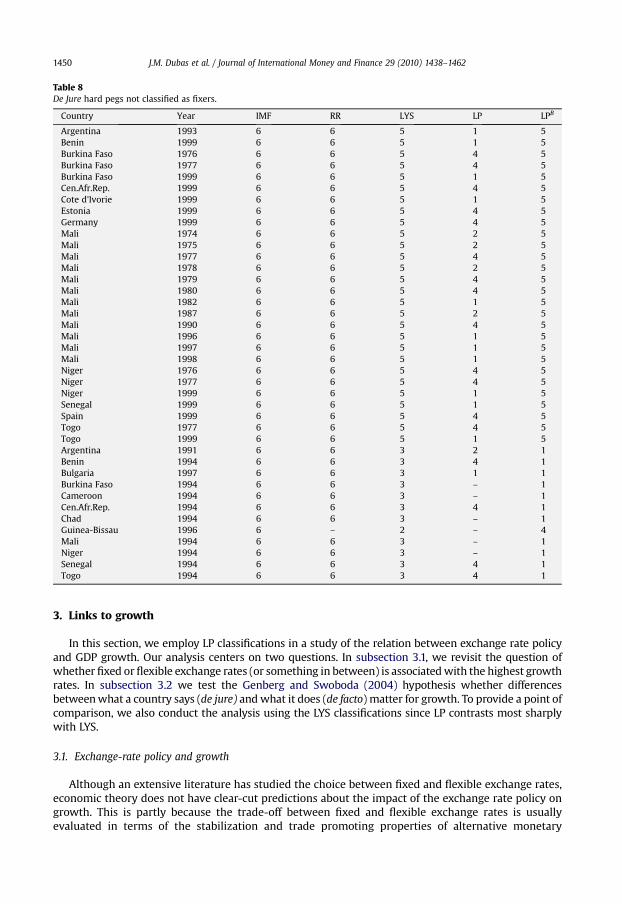
Table 8De Jure hard pegs not classified as fixers.
Country Year IMF RR LYS LP LPB
Argentina 1993 6 6 5 1 5Benin 1999 6 6 5 1 5Burkina Faso 1976 6 6 5 4 5Burkina Faso 1977 6 6 5 4 5Burkina Faso 1999 6 6 5 1 5Cen.Afr.Rep. 1999 6 6 5 4 5Cote d'Ivorie 1999 6 6 5 1 5Estonia 1999 6 6 5 4 5Germany 1999 6 6 5 4 5Mali 1974 6 6 5 2 5Mali 1975 6 6 5 2 5Mali 1977 6 6 5 4 5Mali 1978 6 6 5 2 5Mali 1979 6 6 5 4 5Mali 1980 6 6 5 4 5Mali 1982 6 6 5 1 5Mali 1987 6 6 5 2 5Mali 1990 6 6 5 4 5Mali 1996 6 6 5 1 5Mali 1997 6 6 5 1 5Mali 1998 6 6 5 1 5Niger 1976 6 6 5 4 5Niger 1977 6 6 5 4 5Niger 1999 6 6 5 1 5Senegal 1999 6 6 5 1 5Spain 1999 6 6 5 4 5Togo 1977 6 6 5 4 5Togo 1999 6 6 5 1 5Argentina 1991 6 6 3 2 1Benin 1994 6 6 3 4 1Bulgaria 1997 6 6 3 1 1Burkina Faso 1994 6 6 3 – 1Cameroon 1994 6 6 3 – 1Cen.Afr.Rep. 1994 6 6 3 4 1Chad 1994 6 6 3 – 1Guinea-Bissau 1996 6 – 2 – 4Mali 1994 6 6 3 – 1Niger 1994 6 6 3 – 1Senegal 1994 6 6 3 4 1Togo 1994 6 6 3 4 1
J.M. Dubas et al. / Journal of International Money and Finance 29 (2010) 1438–14621450
3. Links to growth
In this section, we employ LP classifications in a study of the relation between exchange rate policyand GDP growth. Our analysis centers on two questions. In subsection 3.1, we revisit the question ofwhether fixed orflexible exchange rates (or something in between) is associatedwith the highest growthrates. In subsection 3.2 we test the Genberg and Swoboda (2004) hypothesis whether differencesbetweenwhat a country says (de jure) andwhat it does (de facto) matter for growth. To provide a point ofcomparison, we also conduct the analysis using the LYS classifications since LP contrasts most sharplywith LYS.
3.1. Exchange-rate policy and growth
Although an extensive literature has studied the choice between fixed and flexible exchange rates,economic theory does not have clear-cut predictions about the impact of the exchange rate policy ongrowth. This is partly because the trade-off between fixed and flexible exchange rates is usuallyevaluated in terms of the stabilization and trade promoting properties of alternative monetary
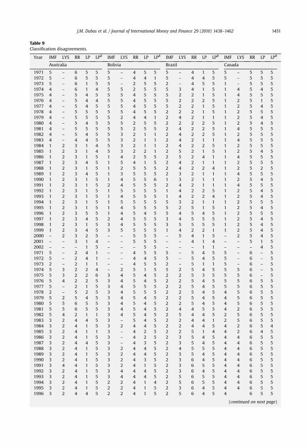
Table 9Classification disagreements.
Year IMF LYS RR LP LPB IMF LYS RR LP LPB IMF LYS RR LP LPB IMF LYS RR LP LPB
Australia Bolivia Brazil Canada
1971 5 – 6 5 5 5 – 4 5 5 5 – 4 1 5 5 – 5 5 51972 5 – 6 5 5 5 – 4 4 1 5 – 4 4 5 5 – 5 5 51973 5 – 6 1 5 5 – 2 5 5 2 – 4 5 5 1 – 5 5 51974 4 – 6 1 4 5 5 2 5 5 5 3 4 1 5 1 4 5 4 51975 4 – 5 4 5 5 5 4 5 5 5 2 2 1 5 1 4 5 5 51976 4 – 5 4 4 5 5 4 5 5 5 2 2 2 5 1 2 5 1 51977 4 – 5 4 5 5 5 4 5 5 5 2 2 1 5 1 2 5 4 51978 4 – 5 5 5 5 5 4 5 5 2 2 2 1 5 1 2 5 5 51979 4 – 5 5 5 5 2 4 4 1 2 4 2 1 1 1 2 5 4 51980 4 – 5 4 5 5 5 2 5 5 2 2 2 2 5 1 2 5 4 51981 4 – 5 5 5 5 5 2 5 5 2 4 2 2 5 1 4 5 5 51982 4 – 5 4 5 5 3 2 1 1 2 4 2 2 5 1 2 5 5 51983 4 – 4 4 5 5 3 2 1 1 2 4 2 1 1 1 4 5 5 51984 1 2 3 1 4 5 3 2 1 1 2 4 2 2 5 1 2 5 5 51985 1 2 3 1 4 5 3 2 2 1 2 5 2 1 5 1 2 5 4 51986 1 2 3 1 5 1 4 2 5 5 2 5 2 4 1 1 4 5 5 51987 1 2 3 4 5 1 5 4 1 5 2 4 2 1 1 1 2 5 5 51988 1 2 3 1 5 1 2 5 5 5 2 4 2 2 4 1 2 5 2 51989 1 2 3 4 5 1 3 5 5 5 2 3 2 1 1 1 4 5 5 51990 1 2 3 1 5 1 4 5 5 6 1 3 2 1 1 1 2 5 4 51991 1 2 3 1 5 2 4 5 5 5 2 4 2 1 1 1 4 5 5 51992 1 2 3 1 5 1 5 5 5 5 1 4 2 2 5 1 2 5 4 51993 1 2 3 1 5 1 4 5 5 5 1 4 2 2 4 1 2 5 4 51994 1 2 3 1 5 1 5 5 5 5 5 3 2 1 1 1 2 5 5 51995 1 2 3 1 5 1 4 5 5 5 5 2 5 1 5 1 2 5 4 51996 1 2 3 5 5 1 4 5 4 5 5 4 5 4 5 1 2 5 5 51997 1 2 3 4 5 2 4 5 5 5 3 4 5 5 5 1 2 5 4 51998 1 2 3 1 5 3 4 5 5 5 3 5 5 5 5 1 2 5 4 51999 1 2 3 4 5 3 5 5 5 5 1 4 2 2 1 1 2 5 4 52000 – 2 3 2 5 – – 5 5 5 – 5 4 1 5 – 2 5 4 52001 – – 3 1 4 – – 5 5 5 – – 4 1 4 – – 5 1 52002 – – – 1 5 – – – 5 5 – – – 1 1 – – – 4 51971 5 – 2 4 1 – – 4 5 5 5 – 5 4 5 5 – 6 – 51972 5 – 2 4 1 – – 4 4 5 5 – 5 4 5 5 – 6 – 51973 2 – 2 1 1 – – 4 5 5 2 – 5 1 1 5 – 6 – 51974 5 3 2 2 4 – 2 5 1 5 5 2 5 4 5 5 5 6 – 51975 5 3 2 2 6 3 4 5 4 5 2 2 5 3 5 5 5 6 – 51976 5 4 2 2 5 3 4 5 4 5 2 2 5 4 5 5 5 6 5 51977 5 – 2 1 5 3 4 5 5 5 2 2 5 4 5 5 5 6 5 51978 2 – 5 2 5 3 4 5 5 5 2 2 5 4 5 4 5 6 5 51979 5 2 5 4 5 3 4 5 4 5 2 2 5 4 5 4 5 6 5 51980 5 5 6 5 5 3 4 5 4 5 2 2 5 4 5 4 5 6 5 51981 5 5 6 5 5 3 4 5 4 5 2 4 4 5 5 4 2 6 5 51982 5 4 2 1 1 3 4 5 4 5 2 5 4 4 5 2 5 6 5 51983 3 2 4 4 5 3 – 5 4 5 2 2 4 4 1 2 5 6 5 51984 3 2 4 1 5 3 2 4 4 5 2 2 4 4 5 4 2 6 5 41985 3 2 4 1 1 3 – 4 2 5 2 2 5 1 4 4 2 6 4 51986 3 2 4 1 5 3 – 4 2 5 2 3 5 4 5 4 4 6 5 51987 3 2 4 4 5 3 – 4 3 5 2 3 5 4 5 4 4 6 5 51988 3 2 4 1 5 3 2 4 4 5 2 4 5 5 5 4 4 6 5 51989 3 2 4 1 5 3 2 4 4 5 2 3 5 4 5 4 4 6 5 51990 3 2 4 1 5 3 2 4 3 5 2 3 6 4 5 4 4 6 5 51991 3 4 4 1 5 3 2 4 1 5 2 3 6 5 5 4 4 6 5 51992 3 2 4 1 5 3 4 4 4 5 2 3 6 4 5 4 4 6 5 51993 3 2 4 1 5 3 4 4 4 5 2 5 6 5 5 4 4 6 5 51994 3 2 4 1 5 2 2 4 1 4 2 5 6 5 5 4 4 6 5 51995 3 2 4 1 5 2 2 4 1 5 2 3 6 4 5 4 4 6 5 51996 3 2 4 4 5 2 2 4 1 5 2 5 6 4 5 4 6 5 5
(continued on next page)
J.M. Dubas et al. / Journal of International Money and Finance 29 (2010) 1438–1462 1451

Table 9 (continued )
Year IMF LYS RR LP LPB IMF LYS RR LP LPB IMF LYS RR LP LPB IMF LYS RR LP LPB
Australia Bolivia Brazil Canada
1997 3 2 4 1 5 2 2 4 1 5 2 5 6 5 5 2 4 2 1 11998 3 2 4 4 5 3 2 4 1 4 3 5 6 1 5 1 4 4 1 11999 1 2 4 1 5 1 2 4 1 4 3 5 6 1 5 1 2 4 4 52000 – 2 4 1 4 – 2 4 1 5 – 5 6 1 4 – 2 4 3 52001 – – 4 1 4 – – 4 4 5 – – 6 5 5 – – 4 4 52002 – – – 1 4 – – – 1 4 – – – 5 5 – – – – 5
J.M. Dubas et al. / Journal of International Money and Finance 29 (2010) 1438–14621452
arrangements and the effect of smoothing cyclical fluctuations and trade creation on growth is not fullyunderstood. Frankel (2003) provides a framework for discussing these trade-offs. We briefly review themain points here.
3.1.1. To fix or to float?Frankel gives four reasons to fix. Beginning with the observation that stable exchange rates provide
a nominal anchor for monetary policy, a policy of fixing can impose the required discipline on themonetary authorities to keep inflation under control and serves as a commitment device to undo theinflationary bias discussed by Barro and Gordon (1983). Second, by reducing uncertainty, maintaining
Table 10Correlations for selected countries.
IMF LYS RR LP LPN
AustraliaEFFVOL �0.43 NA �0.44 �0.54 �0.53NEXRAVOL �0.26 NA �0.31 �0.50 �0.62RESVOL 0.19 NA 0.10 0.39 0.26
BoliviaEFFVOL 0.35 �0.46 �0.50 �0.72 �0.75NEXRAVOL 0.28 �0.35 �0.41 �0.53 �0.59RESVOL �0.10 �0.22 �0.16 0.00 0.02
BrazilEFFVOL �0.22 �0.12 �0.41 �0.42 �0.81NEXRAVOL �0.27 0.00 �0.40 �0.35 �0.86RESVOL �0.42 0.06 �0.25 �0.17 �0.39
CanadaEFFVOL �0.26 �0.56 NA �0.45 NANEXRAVOL �0.27 �0.64 NA �0.52 NARESVOL �0.29 �0.01 NA 0.21 NA
ChileEFFVOL 0.11 0.01 �0.56 0.03 �0.78NEXRAVOL 0.10 �0.01 �0.54 0.07 �0.75RESVOL 0.35 0.17 �0.54 0.03 �0.01
ColumbiaEFFVOL �0.69 �0.55 �0.36 �0.69 �0.81NEXRAVOL �0.76 �0.53 �0.32 �0.75 �0.84RESVOL 0.18 �0.26 �0.19 0.17 0.24
GreeceEFFVOL �0.14 0.32 0.20 �0.34 �0.31NEXRAVOL �0.45 0.13 �0.05 �0.07 �0.31RESVOL �0.18 0.28 0.37 0.26 0.26
ThailandEFFVOL �0.54 �0.23 �0.59 �0.69 �0.84NEXRAVOL �0.60 �0.37 �0.72 �0.87 �0.92RESVOL �0.25 �0.14 �0.04 �0.13 �0.27

J.M. Dubas et al. / Journal of International Money and Finance 29 (2010) 1438–1462 1453
stability in the currency's value can promote increased international trade and investment. Third,maintaining a fix precludes competitive depreciations which can have a destructive effect on trade.Fourth, the exchange rate will not be driven by speculative bubbles if it is fixed.
On the other hand, Frankel also discusses four reasons why countries may want to promoteexchange rate flexibility. First, it allows for an independent monetary policy giving policy makers a toolto offset adverse country shocks. Second, a flexible exchange rate provides an avenue for requiredrelative price adjustments to trade shocks. Third, because a floating rate regime breaks the connectionbetween international reserves and credit creation and allows the central bank to be a lender of lastresort and to retain seigniorage revenues. Fourth, the central bank would not be the target of a spec-ulative attack on its currency.
Given the trade-offs involved, it is perhaps not surprising that empirical results are mixed. However,the weight of the evidence points towards an association between high growth and more stableexchange rates. Indirect evidence is provided by Frankel and Romer (2002) who find that an increase intrade has a significant positive effect on per capita income, and Frankel and Rose (2002) who presentevidence that trade benefits when exchange rates are stabilized. The estimates from the latter paperimply thatmembership in a currency union can raise tradewith other unionmembers by a factor of 3.14
In research that directly examines the relation between exchange rate policies and growth, Ghosh et al.(2002) and RR find higher growth is associated with increased exchange rate stability. Ghosh et al.find that the highest growth rates are associated with intermediate policies, followed by fixers thenfloaters while RR report the growth rank-ordering to be limited flexibility, freely floating, managedfloat and peg.
LYS, on the other hand, find that the highest growth rates are associated with floaters, followed byfixers then intermediate policies. Their results are driven in largely by the experience of non-indus-trialized countries–the growth rate of non-industrialized LYS floaters is approximately 1.1 percenthigher than LYS intermediate and fixer countries. Also, Edwards (2001), who analyzes a much smallerset of countries, reports complementary fragmentary evidence that 'dollarized' countries have grownmore slowly than non-dollarized countries.
3.1.2. A coarse look at the dataWe follow the literature by collapsing our six-way LP exchange rate classification into a three
categories by combining categories 1–2 (floaters), 3–4 (intermediates), and 5–6 (fixers). Table 11displays mean GDP growths sorted by exchange rate policy. Note that categorizing by LYS and LP resultin very different growth rankings. The relative growth performance for the all-countries sample isevidently is driven by the non-industrialized countries as differences in growth rates by LP classifi-cation for industrialized countries are tiny. Mean growth rankings (best to worst) for the all countriesand non-industrialized countries sample sorted by LP are fixers, intermediates and floaters. By LYSclassifications, growth performance is ranked by floaters, fixers and intermediates.
3.1.3. Growth regressionsWe estimate panel data regressions of per capita growth on a standard set of growth determinants
and exchange rate policy dummies. The control variables are generally the same variables employed byLYS. Thus, our control variables include
(i) initial year per capita GDP (1971–1974 average),(ii) initial year population,(iii) population growth,(iv) the investment to GDP ratio,(v) secondary education attainment,(vi) a political indicator of civil liberties,(vii) trade openness,(viii) the change in the terms of trade,
14 Klein (2002) and Klein and Shambaugh (2004) find the effect on trade creation to be somewhat smaller.
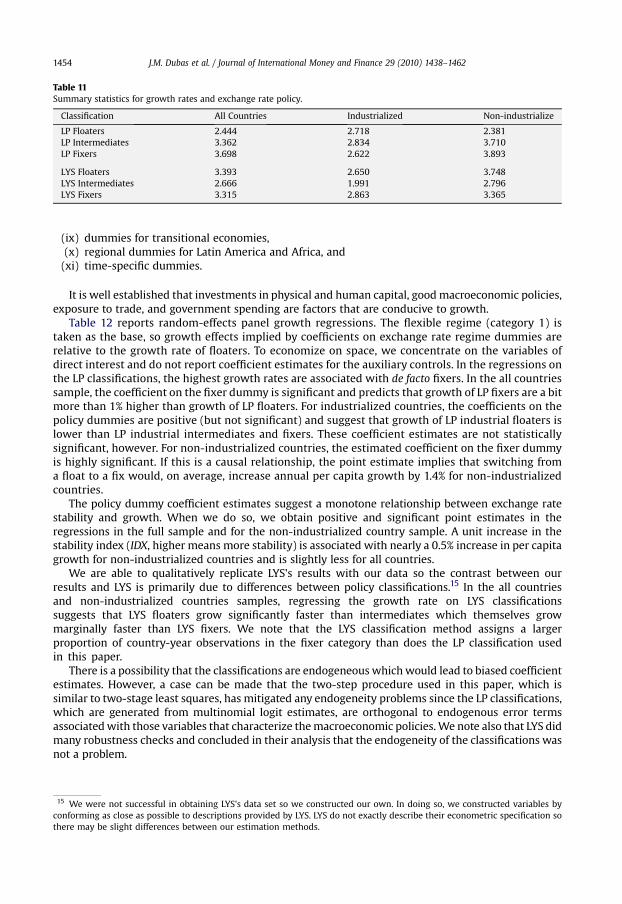
Table 11Summary statistics for growth rates and exchange rate policy.
Classification All Countries Industrialized Non-industrialize
LP Floaters 2.444 2.718 2.381LP Intermediates 3.362 2.834 3.710LP Fixers 3.698 2.622 3.893
LYS Floaters 3.393 2.650 3.748LYS Intermediates 2.666 1.991 2.796LYS Fixers 3.315 2.863 3.365
J.M. Dubas et al. / Journal of International Money and Finance 29 (2010) 1438–14621454
(ix) dummies for transitional economies,(x) regional dummies for Latin America and Africa, and(xi) time-specific dummies.
It is well established that investments in physical and human capital, goodmacroeconomic policies,exposure to trade, and government spending are factors that are conducive to growth.
Table 12 reports random-effects panel growth regressions. The flexible regime (category 1) istaken as the base, so growth effects implied by coefficients on exchange rate regime dummies arerelative to the growth rate of floaters. To economize on space, we concentrate on the variables ofdirect interest and do not report coefficient estimates for the auxiliary controls. In the regressions onthe LP classifications, the highest growth rates are associated with de facto fixers. In the all countriessample, the coefficient on the fixer dummy is significant and predicts that growth of LP fixers are a bitmore than 1% higher than growth of LP floaters. For industrialized countries, the coefficients on thepolicy dummies are positive (but not significant) and suggest that growth of LP industrial floaters islower than LP industrial intermediates and fixers. These coefficient estimates are not statisticallysignificant, however. For non-industrialized countries, the estimated coefficient on the fixer dummyis highly significant. If this is a causal relationship, the point estimate implies that switching froma float to a fix would, on average, increase annual per capita growth by 1.4% for non-industrializedcountries.
The policy dummy coefficient estimates suggest a monotone relationship between exchange ratestability and growth. When we do so, we obtain positive and significant point estimates in theregressions in the full sample and for the non-industrialized country sample. A unit increase in thestability index (IDX, higher means more stability) is associated with nearly a 0.5% increase in per capitagrowth for non-industrialized countries and is slightly less for all countries.
We are able to qualitatively replicate LYS's results with our data so the contrast between ourresults and LYS is primarily due to differences between policy classifications.15 In the all countriesand non-industrialized countries samples, regressing the growth rate on LYS classificationssuggests that LYS floaters grow significantly faster than intermediates which themselves growmarginally faster than LYS fixers. We note that the LYS classification method assigns a largerproportion of country-year observations in the fixer category than does the LP classification usedin this paper.
There is a possibility that the classifications are endogeneous which would lead to biased coefficientestimates. However, a case can be made that the two-step procedure used in this paper, which issimilar to two-stage least squares, has mitigated any endogeneity problems since the LP classifications,which are generated from multinomial logit estimates, are orthogonal to endogenous error termsassociatedwith those variables that characterize themacroeconomic policies.We note also that LYS didmany robustness checks and concluded in their analysis that the endogeneity of the classifications wasnot a problem.
15 We were not successful in obtaining LYS's data set so we constructed our own. In doing so, we constructed variables byconforming as close as possible to descriptions provided by LYS. LYS do not exactly describe their econometric specification sothere may be slight differences between our estimation methods.
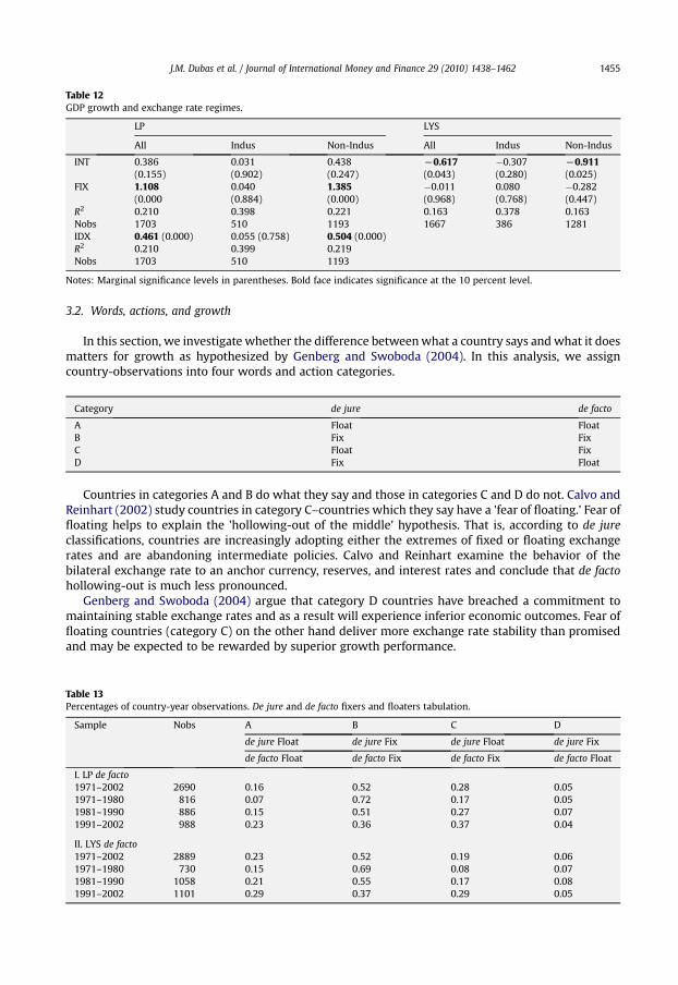
Table 12GDP growth and exchange rate regimes.
LP LYS
All Indus Non-Indus All Indus Non-Indus
INT 0.386 0.031 0.438 L0.617 �0.307 L0.911(0.155) (0.902) (0.247) (0.043) (0.280) (0.025)
FIX 1.108 0.040 1.385 �0.011 0.080 �0.282(0.000 (0.884) (0.000) (0.968) (0.768) (0.447)
R2 0.210 0.398 0.221 0.163 0.378 0.163Nobs 1703 510 1193 1667 386 1281IDX 0.461 (0.000) 0.055 (0.758) 0.504 (0.000)R2 0.210 0.399 0.219Nobs 1703 510 1193
Notes: Marginal significance levels in parentheses. Bold face indicates significance at the 10 percent level.
J.M. Dubas et al. / Journal of International Money and Finance 29 (2010) 1438–1462 1455
3.2. Words, actions, and growth
In this section, we investigate whether the difference betweenwhat a country says and what it doesmatters for growth as hypothesized by Genberg and Swoboda (2004). In this analysis, we assigncountry-observations into four words and action categories.
Category de jure de facto
A Float FloatB Fix FixC Float FixD Fix Float
Countries in categories A and B do what they say and those in categories C and D do not. Calvo andReinhart (2002) study countries in category C–countries which they say have a 'fear of floating.' Fear offloating helps to explain the 'hollowing-out of the middle' hypothesis. That is, according to de jureclassifications, countries are increasingly adopting either the extremes of fixed or floating exchangerates and are abandoning intermediate policies. Calvo and Reinhart examine the behavior of thebilateral exchange rate to an anchor currency, reserves, and interest rates and conclude that de factohollowing-out is much less pronounced.
Genberg and Swoboda (2004) argue that category D countries have breached a commitment tomaintaining stable exchange rates and as a result will experience inferior economic outcomes. Fear offloating countries (category C) on the other hand deliver more exchange rate stability than promisedand may be expected to be rewarded by superior growth performance.
Table 13Percentages of country-year observations. De jure and de facto fixers and floaters tabulation.
Sample Nobs A B C D
de jure Float de jure Fix de jure Float de jure Fix
de facto Float de facto Fix de facto Fix de facto Float
I. LP de facto1971–2002 2690 0.16 0.52 0.28 0.051971–1980 816 0.07 0.72 0.17 0.051981–1990 886 0.15 0.51 0.27 0.071991–2002 988 0.23 0.36 0.37 0.04
II. LYS de facto1971–2002 2889 0.23 0.52 0.19 0.061971–1980 730 0.15 0.69 0.08 0.071981–1990 1058 0.21 0.55 0.17 0.081991–2002 1101 0.29 0.37 0.29 0.05
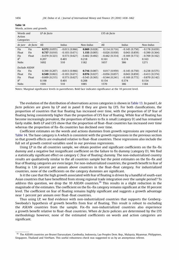
Table 14Words, actions and growth.
Words andActionCategories
LP de facto LYS de facto
de jure de facto All Indus Non-Indus All Indus Non-Indus
Fix Fix 0.572 (0.055) �0.013 (0.966) 0.869 (0.028) 0.114 (0.716) �0.145 (0.750) �0.178 (0.659)Float Fix 0.737 (0.010) �0.103 (0.671) 1.155 (0.005) �0.026 (0.930) 0.043 (0.859) �0.390 (0.364)Fix Float �0.479 (0.323) 0.573 (0.627) �0.402 (0.492) �0.442 (0.314) �0.169 (0.772) �0.769 (0.162)R2 0.207 0.401 0.218 0.161 0.374 0.163Nobs 1692 510 1182 1657 386 1271
Exclude ASEANFix Fix 0.390 (0.207) �0.013 (0.966) 0.716 (0.087) 0.017 (0.959) �0.145 (0.750) �0.238 (0.575)Float Fix 0.549 (0.063) �0.103 (0.671) 0.976 (0.027) �0.056 (0.857) 0.043 (0.859) �0.413 (0.374)Fix Float �0.609 (0.215) 0.573 (0.627) �0.545 (0.365) �0.544 (0.241) �0.169 (0.772) �0.870 (0.142)R2 0.198 0.401 0.208 0.154 0.374 0.154Nobs 1595 510 1085 1570 386 1184
Notes: Marginal significance levels in parentheses. Bold face indicates significance at the 10 percent level.
J.M. Dubas et al. / Journal of International Money and Finance 29 (2010) 1438–14621456
The evolution of the distribution of observations across categories is shown in Table 13. In panel I, defacto policies are given by LP and in panel II they are given by LYS. For both classifications, theproportion of countries that fear floating has increased over time, with the proportion of LP fear offloating being consistently higher than the proportion of LYS fear of floating. While fear of floating hasbecome increasingly prevalent, the proportion of failures to fix is small (category D) and has remainedfairly stable. Both LP and LYS show that the proportion of float–float countries has increased over timewhereas the proportion of fix–fix countries has declined over time.
Coefficient estimates on the words and actions dummies from growth regressions are reported inTable 14. The base category is Awhich is consistent with the growth regressions in the previous sectionso that growth effects are evaluated relative to float–float countries. These regressions also include thefull set of growth control variables used in our previous regressions.
Using LP in the all countries sample, we obtain positive and significant coefficients on the fix–fixdummy and a negative but insignificant coefficient on the failure to fix dummy (category D). We finda statistically significant effect on category C (fear of floating) dummy. The non-industrialized countryresults are qualitatively similar to the all countries sample but the point estimates on the fix–fix andfear of floating categories are even larger. For non-industrialized countries, the growth benefit to fear offloating is 1.16 percent per annum above countries in the float–float category. For industrializedcountries, none of the coefficients on the category dummies are significant.
Is it the case that the high growth associatedwith fear of floating is driven by a handful of south-eastAsian countries that have benefitted from strong regional trade integration over the sample period? Toaddress this question, we drop the 10 ASEAN countries.16 This results in a slight reduction in themagnitude of the estimates. The coefficient on the fix–fix category remains significant at the 10 percentlevel. The coefficient on fear of floating remains highly significant and suggests a growth advantagenear 1 percent per annum over float–float countries.
Thus using LP, we find evidence with non-industrialized countries that supports the Genberg-Swoboda's hypothesis of growth benefits from fear of floating. This result is robust to excludingthe ASEAN countries from the sample. Fix–fix non-industrialized countries also experiencea growth benefit relative to float–float countries. When de facto policies are determined by the LYSmethodology however, none of the estimated coefficients on words and action categories aresignificant.
16 The ASEAN countries are Brunei Darussalam, Cambodia, Indonesia, Lao Peoples Dem. Rep., Malaysia, Myanmar, Philippines,Singapore, Thailand and VietNam. This useful robustness check was suggested to us by an anonymous referee.
J.M. Dubas et al. / Journal of International Money and Finance 29 (2010) 1438–1462 1457
4. Conclusion
This paper has proposed an econometric approach to classifying exchange rate policy. The proce-dure has three attractive features: First, it is based on tools that are familiar to economists. Second, itcan be replicated, modified, and updated in a straightforward manner. Third, it produces sensibleresults. In producing the classifications, we employed information contained in the country's effectiveexchange rate. The use of the effective exchange rate in our analysis leads to an improvement inclassifying policies and underscores the value in taking a multilateral approach in forming a general-ized assessment of national policy towards exchange rate management.
Our investigation of the impact of exchange rate policies and growth found that the highest growthto be associated with de facto fixers. This is in line with much of the extant literature and is consistentwith research that has found trade benefits from currency blocs. Whether the growth advantages thatwe find are the result of maintaining a stable currency per se or from selection of countries that aremembers of trade and currency blocs is unanswered but is a problem for future research.
While the exchange rate regime adopted de facto appears to matter for growth, we also findevidence that a more nuanced representation of policy based on the fear of floating concept matters.Point estimates imply a rank-ordering of GDP growth from highest to lowest for categories: i) de jurefloaters–de facto fixers, ii) de jure fixers–de facto fixers, iii) de jure floaters–de facto floaters, and iv) dejure fixers–de facto floaters. Countriesmay have a good reason to display fear of floating since those thatdo experience significantly higher per capita growth.
Appendix
The Data
Our primary data source is the International Monetary Fund's International Financial Statisticsdatabase. Our data set includes 180 countries, each with a unique country code (1–180). Country code182 represents the world, country code 181 represents residuals, or countries not included in the 180.
Due to hyper-inflations and hyper-depreciations of local currencies for several countries, the realGDP data from source seemed unreliable. (For several countries, per capita real GDP in 1971 US dollarswas less than 1 cent per year.) Therefore, we decided to convert real per capita local currency GDP intoconstant 2000 US dollars, using the bilateral exchange rate to the USD in 2000. Then in the empiricalwork, we dropped observations for which this real per capita GDP was less than $3 (about 6 percent ofthe sample). The country-year observations that we excluded are: Congo, Dem. Rep: 1971–1998,Belarus: 1987–2000, Turkmenistan: 1987–2000, Tajikistan: 1985–2000, Ukraine: 1987–2000, Ghana:1971–2000, Sudan: 1971–2000, Equador: 1971–2000, Guinea-Bissau: 1971–2000, Surinam: 1971–2000, Bulgaria: 1980–2000, Afghanistan: 1971–1982.
Other notes: Fmr. Rep of Vietnam included as Vietnam in sample (cc 176), Fmr. Fed Rep of Germany(West Germany) included as Germany in sample (cc 66), Aruba, Netherlands Antilles defined togetheras Netherlands Antilles (cc 8) until 1987, separate thereafter, Fmr. Dem Yemen defined as Yemen insample (cc 177), East and West Pakistan defined as Pakistan in sample (cc 124)
A monthly data set extending from 1960.01 to 2002.12 was used to construct annual volatilitymeasures and other pieces of the annual data set. The monthly data set is comprised of the following.
Net Reserves: (in US$) (IFS line 1L.DZF) When this data was clearly reported on a quarterly basis (i.e., atleast 2 consecutive periods), the datawas interpolated to get monthly data points. A full list is availableupon request. Some data anomalies were discovered in the raw data. Negative reserves were observedfor several months for the Central African Republic, Chad, Gabon. Negative reserves in only one monthwere reported for Congo, Guinea-Bissau, and Ukraine. Except for the Ukraine, these are all Central FrancZone countries.
WE note that this is not the same definition of reserves as that reported by LYS. We attempted to re-create their reserve data. They describe it as the foreign assets less foreign liabilities and centralgovernment deposits (IFS: line 11, line 16c, line 16d). These data contained many anomaliesdLYS
J.M. Dubas et al. / Journal of International Money and Finance 29 (2010) 1438–14621458
reserves are negative for 30 percent of all observations and data are partially or entirely missing formany important countries (Australia, Belgium, Brazil, France, Greece, Japan, New Zealand, Norway,Switzerland, United Kingdom). The reserve measure we utilize has approximately 10,000 moreobservations than LYS.
Nominal exchange rate: 2 bilateral (US$) measures as in annual data.Nominal effective exchange rates: Using trade weights from Comtrade data set. Additionally, to givethese time series properties, they were smoothed using a 12 month moving average (5 lags, 6 leads,including observation).CPI: IFS (line 64..ZF) No monthly data available for USSR, Czechoslovakia. Russian monthly CPI dataderived from IFS data (CPI change over previous period, line 64XX..ZF), and inserted into database. InAustralia, Belize, New Zealand, Papua New Guinea, Vanuatu, the CPI is reported quarterly. Thesequarterly data were interpolated to obtain monthly measures using Q1 as month 3, Q2 as month 6,Q3as month 9, Q4 as month 12.Investment derived by using GDP (current Local currency units (LCU)) minus external balance on goodsand services minus final consumption expenditure [I ¼ GDP-NX-C] (all from World DevelopmentIndicators).Population, GDP, Exports, Imports, Terms of trade (Exports as a capacity to import), obtained fromWDI.Secondary education: WDI. Data is generally reported every 5 years in the data source which waslinearly interpolated to obtain annual observations.Civil liberties: Following LYS, these data were obtained from Freedom House country rankings.
Properties of effective and bilateral exchange rates
Past research has typically emphasized the properties of the bilateral exchange rate of an anchorcurrency in connection with policies classification [Calvo and Reinhart (2002), Reinhart and Rogoffet al. (2003), Levy-Yeyati and Sturzenegger (2003), Shambaugh (2004)]. The informal comparisonbetween effective and bilateral nominal exchange rates presented in this section shows that a verydifferent picture about both the level and the volatility of a country's currency value can emergedepending onwhether it is viewed through the lens of a bilateral or a multilateral exchange rate. Theirproperties are sufficiently different for us to conclude that the effective exchange rate containsinformation beyond that contained in the bilateral exchange rate that is relevant for a country inannouncing the de jure regime that describes how it manages its currency.
Anchor currencies for bilateral exchange rates are either the US dollar, the British pound, the Frenchfranc, or the German mark. For this, we follow the country assignment used in LYS. Because effectiveexchange rate series do not exist for most non-industrialized countries, these data are constructed byus.17We divide our discussion between an examination of the volatility of the alternative exchange ratemeasures and a comparison of their dynamics.
Volatility
We measure volatility as the annual sample standard deviation of monthly percentage changes inthe exchange rate. The effective and bilateral exchange rate will exhibit the same degree of stabilityonly if the country does all of its trade with the country to which it fixes or trades only with countries
17 We begin with aggregated trade data obtained from the United Nation's Comtrade database. These are imports and exportsaccording to SITC rev.1 commodity classification or SITC rev.2 data when SITC rev.1 was not available for a particular country/year. For each reporting country i ¼ 1, ., 180 and year (t ¼ 1971, ., 2002), set of weights are formed by taking trade betweencountry i and j as a fraction of country i's total trade for that year. These weights are used to construct the geometric average ofrespective bilateral nominal exchange rates and normalized such that their value in December 2000 is 100 to form the effectiveexchange rate. The NEER for country i at month m of year t is constructed as: NEERimt
¼ QNj¼1ðBNEijmt
Þwijt where NEERimtis the
nominal effective exchange rate for country i at month m of year t, BNEijmtis the nominal bilateral exchange rate between
country i and j at monthm of year t calculated as the relative rates per U.S. dollar, wijt is the trade weight between county i and jat year t, and N is total number of countries.
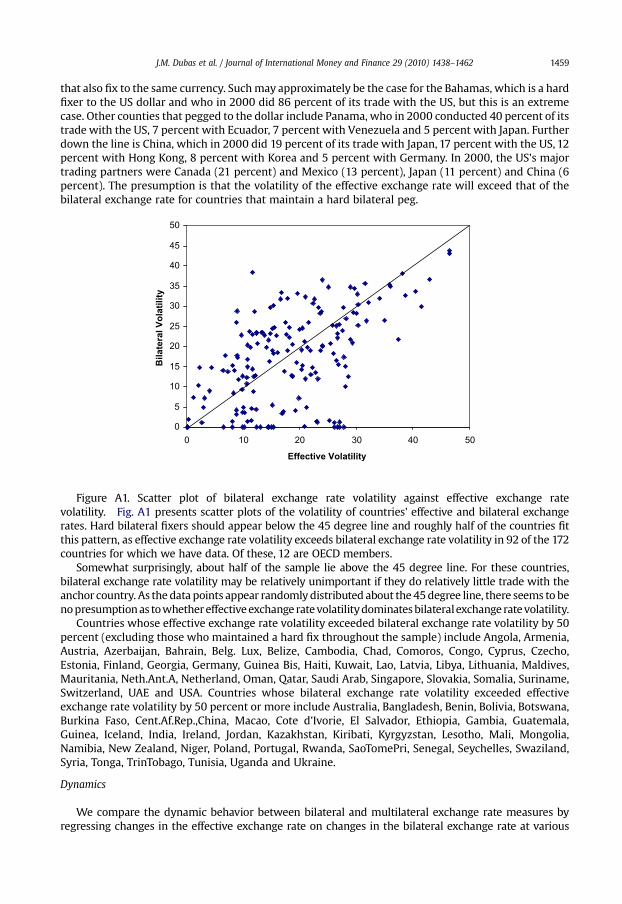
J.M. Dubas et al. / Journal of International Money and Finance 29 (2010) 1438–1462 1459
that also fix to the same currency. Suchmay approximately be the case for the Bahamas, which is a hardfixer to the US dollar and who in 2000 did 86 percent of its trade with the US, but this is an extremecase. Other counties that pegged to the dollar include Panama, who in 2000 conducted 40 percent of itstrade with the US, 7 percent with Ecuador, 7 percent with Venezuela and 5 percent with Japan. Furtherdown the line is China, which in 2000 did 19 percent of its trade with Japan, 17 percent with the US, 12percent with Hong Kong, 8 percent with Korea and 5 percent with Germany. In 2000, the US's majortrading partners were Canada (21 percent) and Mexico (13 percent), Japan (11 percent) and China (6percent). The presumption is that the volatility of the effective exchange rate will exceed that of thebilateral exchange rate for countries that maintain a hard bilateral peg.
0
5
10
15
20
25
30
35
40
45
50
0 10 20 30 40 50
Effective Volatility
Bilateral V
olatility
Figure A1. Scatter plot of bilateral exchange rate volatility against effective exchange ratevolatility. Fig. A1 presents scatter plots of the volatility of countries' effective and bilateral exchangerates. Hard bilateral fixers should appear below the 45 degree line and roughly half of the countries fitthis pattern, as effective exchange rate volatility exceeds bilateral exchange rate volatility in 92 of the 172countries for which we have data. Of these, 12 are OECD members.
Somewhat surprisingly, about half of the sample lie above the 45 degree line. For these countries,bilateral exchange rate volatility may be relatively unimportant if they do relatively little trade with theanchor country. As the data points appear randomlydistributed about the 45degree line, there seems tobenopresumptionas towhethereffectiveexchange ratevolatilitydominatesbilateralexchange ratevolatility.
Countries whose effective exchange rate volatility exceeded bilateral exchange rate volatility by 50percent (excluding those who maintained a hard fix throughout the sample) include Angola, Armenia,Austria, Azerbaijan, Bahrain, Belg. Lux, Belize, Cambodia, Chad, Comoros, Congo, Cyprus, Czecho,Estonia, Finland, Georgia, Germany, Guinea Bis, Haiti, Kuwait, Lao, Latvia, Libya, Lithuania, Maldives,Mauritania, Neth.Ant.A, Netherland, Oman, Qatar, Saudi Arab, Singapore, Slovakia, Somalia, Suriname,Switzerland, UAE and USA. Countries whose bilateral exchange rate volatility exceeded effectiveexchange rate volatility by 50 percent or more include Australia, Bangladesh, Benin, Bolivia, Botswana,Burkina Faso, Cent.Af.Rep.,China, Macao, Cote d'Ivorie, El Salvador, Ethiopia, Gambia, Guatemala,Guinea, Iceland, India, Ireland, Jordan, Kazakhstan, Kiribati, Kyrgyzstan, Lesotho, Mali, Mongolia,Namibia, New Zealand, Niger, Poland, Portugal, Rwanda, SaoTomePri, Senegal, Seychelles, Swaziland,Syria, Tonga, TrinTobago, Tunisia, Uganda and Ukraine.
Dynamics
We compare the dynamic behavior between bilateral and multilateral exchange rate measures byregressing changes in the effective exchange rate on changes in the bilateral exchange rate at various
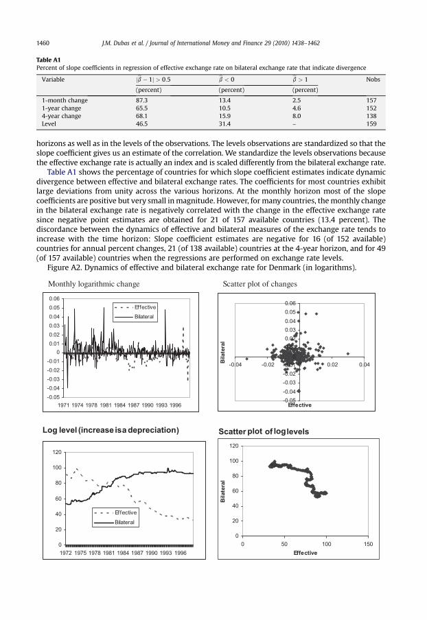
Table A1Percent of slope coefficients in regression of effective exchange rate on bilateral exchange rate that indicate divergence
Variable jbb � 1j > 0:5 bb < 0 bb > 1 Nobs
(percent) (percent) (percent)
1-month change 87.3 13.4 2.5 1571-year change 65.5 10.5 4.6 1524-year change 68.1 15.9 8.0 138Level 46.5 31.4 – 159
J.M. Dubas et al. / Journal of International Money and Finance 29 (2010) 1438–14621460
horizons as well as in the levels of the observations. The levels observations are standardized so that theslope coefficient gives us an estimate of the correlation. We standardize the levels observations becausethe effective exchange rate is actually an index and is scaled differently from the bilateral exchange rate.
Table A1 shows the percentage of countries for which slope coefficient estimates indicate dynamicdivergence between effective and bilateral exchange rates. The coefficients for most countries exhibitlarge deviations from unity across the various horizons. At the monthly horizon most of the slopecoefficients are positive but very small inmagnitude. However, for many countries, themonthly changein the bilateral exchange rate is negatively correlated with the change in the effective exchange ratesince negative point estimates are obtained for 21 of 157 available countries (13.4 percent). Thediscordance between the dynamics of effective and bilateral measures of the exchange rate tends toincrease with the time horizon: Slope coefficient estimates are negative for 16 (of 152 available)countries for annual percent changes, 21 (of 138 available) countries at the 4-year horizon, and for 49(of 157 available) countries when the regressions are performed on exchange rate levels.
Figure A2. Dynamics of effective and bilateral exchange rate for Denmark (in logarithms).
Monthly logarithmic change Scatter plot of changes
-0.05-0.04-0.03-0.02-0.010
0.010.020.030.040.050.06
1971 1974 1978 1981 1984 1987 1990 1993 1996
Effective
Bilateral
-0.05-0.04-0.03-0.02-0.010
0.010.020.030.040.050.06
-0.04 -0.02 0 0.02 0.04
Effective
Bilateral
Log level (increase isa depreciation) Scatter plot of loglevels
0
20
40
60
80
100
120
1972 1975 1978 1981 1984 1987 1990 1993 1996
Effective
Bilateral
0
20
40
60
80
100
120
0 50 100 150Effective
Bil
ateral

J.M. Dubas et al. / Journal of International Money and Finance 29 (2010) 1438–1462 1461
Looking only at the correlation between changes in the effective and bilateral exchange rates will insome cases obscure an underlying divergence in their trends, which is illustrated in the case ofDenmark. Fig. A2 shows plots of the monthly percent change, 4-year percent change and the levels ofeffective and bilateral exchange rates for Denmark. The reciprocal of nominal effective exchange ratesare plotted. Therefore, the decrease of NEER represents appreciation of effective rate. Both effectiverates and bilateral rate are normalized in the plot. While there has been an effective appreciation of thekrone over the sample period and a bilateral depreciation with respect to the deutschemark, first-differences in the two exchange rate measures are positively correlated.18 The effective and bilateralexchange rates for Canada and many European countries exhibit similar patterns (not shown).
The descriptive statistics that we report combine experiences across policies ranging from hyper-inflation to currency board hard fixes. What these very aggregative summary statistics on volatilitysuggest, however, is that a very different picture about exchange volatility exposure emerges whenviewed through the lens of effective rather than bilateral exchange rates.
Multinomial logit estimation results
Here, we report the multinomial logit estimation results that underlies the 'logit policy' classifi-cations. A normalizationwith respect to one of the regimes is required for identification.We use regime5 for this normalization since it is the regime that occurs most frequently.
Table A2Multinomial logit estimates for logit policy classifications.
Coef. s.e. t-ratio Coef. s.e. t-ratio
Regime 1 Regime 2EV1 �0.317 0.108 �2.94 EV1 �0.392 0.110 �3.57EV2 0.359 0.145 2.48 EV2 0.277 0.149 1.85BV2 1.700 0.106 16.08 BV2 1.781 0.106 16.82RV �0.056 0.009 �6.2 RV �0.039 0.008 �4.61Const �1.292 0.138 �9.34 Const �1.354 0.139 �9.72
Regime 3 Regime 4EV1 �0.546 0.130 �4.19 EV1 0.042 0.135 0.31EV2 0.003 0.172 0.02 EV2 �1.089 0.212 �5.1BV2 1.889 0.107 17.61 BV2 1.874 0.105 17.8RV �0.067 0.010 �6.42 RV �0.025 0.007 �3.34Const �0.840 0.150 �5.59 Const �0.420 0.137 �3.06
Regime 6EV1 �0.255 0.159 �1.61EV2 0.115 0.197 0.58BV2 0.0600 0.152 0.4RV 0.0212 0.007 3.11Const �1.091 0.159 �6.84
References
Alesina, A., Wagner, A., 2003. Choosing (and reneging on) Exchange Rate Regimes. NBER Working Paper 9809.Barro, R.J., Gordon, D.B., 1983. A positive theory of monetary policy in a natural rate model. Journal of Political Economy 91,
589–610.Bordo, M.D., Flandreau, M., 2001. Core, Periphery, Exchange Rate Regimes, and Globalization. NBER Working Paper 8584.Broda, C., 2004. Terms of trade and exchange rate regimes in developing countries. Journal of International Economics 63,
31–58.
18 Two trend-stationary series {xt} and {yt} can trend in opposite directions and have positively correlated changes if the timeswhen both series increase xt experiences large changes and yt experiences small changes and vice-versa when both seriesdecrease. Suppose that yt ¼ að1� rÞ þ ryt�1 þ 3t ; xt ¼ bð1� gÞ þ gxt�1 þ vt ; ð3t ; vtÞ0 wiid ð0;PÞ;P11 ¼ P
22 ¼ 1;P
12 > 0;0 < r;g < 1: Let a< 0 and b> 0 so that they trend in opposite directions. Denoting the deviation from the mean with a ' w ', itfollows that the covariance between changes in xt and yt is EðD~ytD~xtÞ ¼ ð1� grÞ�1S12ð2� g� rÞ > 0.

J.M. Dubas et al. / Journal of International Money and Finance 29 (2010) 1438–14621462
Calvo, G.A., Reinhart, C.M., 2002. Fear of floating. Quarterly Journal of Economics CXVII (117), 379–408.Edwards, S., 2001. Dollarization and Economic Performance: An Empirical Investigation. NBER working Paper 8274.Edwards, S., Levy-Yeyati, E., 2003. Flexible Exchange Rates as Shock Absorbers. NBER Working Paper 9867.Frankel, J.A., 2003. Experience of and Lessons from Exchange Rate Regimes in Emerging Economies. NBER Working Paper
10032.Frankel, J.A., Schmukler, S.L., Serven, L., 2002. Global Transmission of Interest Rates: Monetary Independence and Currency
Regime. NBER Working Paper 8828.Frankel, J.A., Romer, D., 2002. Does trade cause growth? American Economic Review 89, 379–399.Frankel, J.A., Rose, A., 2002. An estimate of the effect of common currencies on trade and income. Journal of International
Economics 117, 437–466.Frankel, J.A., Wei, S.J., 1995. Emerging currency blocs. In: Genberg, H. (Ed.), The International Monetary System: Its Institutions
and Its Future. Springer, Berlin, pp. 111–143.Genberg, H., Swoboda, A.K., 2004. Exchange-Rate Regimes: Does What Countries Say Matter? mimeo Graduate Institute of
International Studies, Geneva, Switzerland.Ghosh, A.A., Gulde, A., Ostry, J.D., Wolf, H., 2002. Exchange Rate Regimes: Choices and Consequences. MIT Press.Juhn, G.S., Mauro, P., 2002. Long-Run Determinants of Exchange Rate Regimes: A Simple Sensitivity Analysis. IMF Working
Paper 02/104.Klein, M.W., 2002. Dollarization and Trade. NBER Working Paper 8876.Klein, M.W., Shambaugh, J.C., 2004. Fixed Exchange Rates and Trade. NBER Working Paper 10696.Levy-Yeyati, E., Sturzenegger, F., 2003. To float or to fix: evidence on the impact of exchange rate regimes on growth. American
Economic Review 93, 1173–1193.McFadden, D., 1974. The measurement of urban travel demand. Journal of Public Economics 3, 303–328.Reinhart, C.M., Rogoff, K.S., 2004. The modern history of exchange rate arrangements: a reinterpretation. Quarterly Journal of
Economics.Reinhart, C.M., Rogoff, K.S., Savastano, M.A. 2003. Addicted to Dollars. NBER Working Paper 10015.Rogoff, K.S., Husain, A.M., Mody, A., Brooks, R.J., Oomes, N., 2003. Evolution and Performance of Exchange Rate Regimes. IMF
Working Paper 03/243.Schmidt, P., Strauss, R., 1975. The prediction of occupation using multinomial logit models. International Economic Review 16,
471–486.Shambaugh, J.C., 2004. The effect of fixed exchange rates on monetary policy. Quarterly Journal of Economics 119, 301–352.
Related Documents