A moving grid finite element method applied to - Mathematical Institute

Journal of Computational Physics 190 (2003) 478–500

www.elsevier.com/locate/jcp

A moving grid finite element method applied to amodel biological pattern generator q

Anotida Madzvamuse a,*, Andrew J. Wathen b, Philip K. Maini c

a Mathematics Department, 221 Parker Hall, Auburn University, AL 36849-3510, USAb Numerical Analysis Group, Oxford University Computing Laboratory, Wolfson Building, Parks Road, Oxford OX1 3QD, UK

c Centre for Mathematical Biology, Mathematical Institute, University of Oxford, 24–29 St. Giles’, Oxford OX1 3LB, UK

Received 2 September 2002; received in revised form 10 April 2003; accepted 26 May 2003

Abstract

Many problems in biology involve growth. In numerical simulations it can therefore be very convenient to employ a

moving computational grid on a continuously deforming domain. In this paper we present a novel application of the

moving grid finite element method to compute solutions of reaction–diffusion systems in two-dimensional continuously

deforming Euclidean domains. A numerical software package has been developed as a result of this research that is

capable of solving generalised Turing models for morphogenesis.

� 2003 Elsevier B.V. All rights reserved.

Keywords: Moving grid finite elements; Reaction–diffusion systems; Turing instability; Colour pattern formation; Butterfly wing;

Papilio dardanus

1. Introduction

Understanding how spatial pattern arises is a central but still unresolved issue in developmental biology.

It is clear that genes play a crucial role in embryology but the study of genetics alone can not explain how

the complex mechanical and chemical spatio-temporal signalling cues which determine cell fate are set upand regulated in the early embryo. These signals are a consequence of many nonlinear interactions and

mathematical modelling and numerical computation have an important role to play in understanding and

predicting the outcome of such complex interactions.

The application of mathematical modelling to problems in developmental biology has given rise to a

variety of models which account for spatio-temporal patterning phenomena. In the chemical prepattern

model approach it is hypothesised that a spatially homogeneous or uniform density of cells responds to

some spatially heterogeneous chemical pattern and differentiates according to some rules. Turing [49] in his

qThis work supported by EPSRC Life Sciences Initiative Grant GR/R03914.*Corresponding author. Fax: +1-334-844-6555.

E-mail address: [email protected] (A. Madzvamuse).

0021-9991/$ - see front matter � 2003 Elsevier B.V. All rights reserved.

doi:10.1016/S0021-9991(03)00294-8

mail to: [email protected]

A. Madzvamuse et al. / Journal of Computational Physics 190 (2003) 478–500 479

seminal paper concerning morphogenesis, suggested a novel concept of diffusion driven instability in re-

action–diffusion systems. Since then, the reaction–diffusion theory of pattern formation has been widely

applied to biology, ecology [42], semiconductor physics [6], material science [23], hydrodynamics [50], as-

trophysics [35], chemistry and economics. Typical examples of biological applications of reaction–diffusion

systems are: pattern formation in hydra [19], animal coat markings [32], butterfly wing pigmentation

patterns [34], skeletal patterning in limb development (see for review [27]) and shell pigmentation patterns

[28]. Detailed studies of these models have been carried out on spatial domains of one dimension and two

dimensions with simple geometries. In nearly all these cases, the domain was considered fixed in size,however recent experimental evidence shows that domain growth may play a crucial role in pattern

formation [22].

From the biologically realistic assumption that growth occurs via a continuous deformation of the

domain, we can solve the system numerically using the finite element method on a continuously deforming

domain [4]. The essential component underlying this method is the representation of the object function by

a piecewise linear continuous function on a finite element mesh in which the nodal positions vary with time.

The way in which these nodes are moved and how the solution evolves is derived in the weak form of the

model system. The nodal movement can either be provided by a separate definition or by a mechanism: wewill prescribe a specific definition for the motion of the domain and correspondingly define the motion of all

the nodes in the grid. This is the key difference to the moving finite element method invented by Miller [29].

Miller does not specify the motion of the nodes, instead the nodal movement is generated automatically by

minimising the residual of the differential equation. In his method mesh tangling may result whereas this

can be avoided with prescribed mesh motion (see [12,13] for more details on mesh tangling and other

problems). Although our work will be mainly on a two-dimensional moving grid, Sun W. [46], use the

moving mesh method to solve the one-dimensional Gierer–Meinhardt model.

In Section 2 we present the model equations considered in this paper. The moving grid finite elementtheory is described in Section 3. Here we derive the weak form of the partial differential equation and

describe the Galerkin finite element approximation on a continuously deforming grid. Numerical experi-

ments are presented in Section 4 on regular and irregular growing domains. Lastly in Section 5 we present

conclusions and discuss the implications of the novel application of the moving finite element method to

pattern formation and transition in biological problems. We also provide numerical software and docu-

mentation for the methods described in this paper which can be freely downloaded from http://web.com-

lab.ox.ac.uk/oucl/work/andy.wathen/software.html.

2. Model equations

The numerical experiments in this paper will be restricted to a generalised reaction–diffusion system of

two chemical species which can be written in terms of non-dimensional variables as

ou

ot¼ cfðuÞ þ P3ðuÞ þDr2u in XðtÞ; ð2:1Þ

with XðtÞ representing a time-dependent domain. Here we define

u ¼u

v

� �; f ¼

f ðu; vÞgðu; vÞ

� �; P3 ¼

p3ðu; vÞq3ðu; vÞ

� �; D ¼

Du 0

0 Dv

� �; x ¼ xðtÞ; yðtÞð Þ;

where u; v are the two chemical concentrations under investigation, f ; g; p3; q3 are reaction kinetics, and D is

the diffusion matrix (Du and Dv are constant diffusion parameters). In a number of important applications

the parameters c and d are the most important and this is why they are explicitly included in (2.1).

http://web.comlab.ox.ac.uk/oucl/work/andy.wathen/software.html


480 A. Madzvamuse et al. / Journal of Computational Physics 190 (2003) 478–500

Initial conditions are given by uðx; 0Þ ¼ u0ðxÞ where u0ðxÞ is a prescribed non-negative continuous

bounded function. Boundary conditions can be of Dirichlet type (u and/or v given on the boundary) or of

(homogeneous) Neumann type which describe zero-flux of u (or v) out of the boundary. Initial conditions

are defined as small random perturbations about the uniform homogeneous steady state, if it exists (i.e., a

state u ¼ constant, v ¼ constant satisfying the boundary conditions and equations (2.1)).

Below we consider three special cases where c 6¼ 0 and p3ðu; vÞ ¼ 0 ¼ q3ðu; vÞ. In each case we give a brief

description of each model and its physical interpretation.

2.1. Gierer–Meinhardt reaction kinetics

This is a phenomenological model suggested by Gierer and Meinhardt [19] whereby reaction kinetics are

chosen in such a way that one of the chemicals (termed activator) activates the production of the otherchemical (the inhibitor) which, in turn, inhibits the production of the activator. The non-dimensionalised

reaction–diffusion system is given by

ouot

¼ c a�

� buþ u2

vð1þ ku2Þ

�þr2u; ð2:2Þ

ovot

¼ c u2�

� v�þ dr2v; ð2:3Þ

where uðx; y; tÞ is the concentration of the activator, vðx; y; tÞ is the concentration of the inhibitor, t is time

and r2 ¼ ðo2=ox2Þ þ ðo2=oy2Þ is the two-dimensional Laplacian. a, b, d and c are all non-dimensionalisedpositive parameters and k is a measure of the saturation concentration (see for example [33]). The biological

interpretation of the reaction kinetics in (2.2) is that u is produced at a constant rate ca and is degraded

linearly at rate cb. The c½u2=vð1þ ku2Þ� term implies autocatalysis in u with saturation at high concentration

values of u, and inhibition of u through the production of v. In Eq. (2.3), v is activated (produced) by u and

degraded linearly.

2.2. Thomas reaction kinetics

This model is based on a specific substrate–inhibition reaction involving the substrates oxygen (vðx; y; tÞ)and uric acid (uðx; y; tÞ) which react in the presence of the enzyme uricase. The reaction kinetics, derived by

fitting the kinetics to experimental data [47], can be written in non-dimensional form as

ouot

¼ c að � u� hðu; vÞÞ þ r2u; ð2:4Þ

ovot

¼ c abð � av� hðu; vÞÞ þ dr2v ð2:5Þ

with hðu; vÞ ¼ quv=ð1þ uþ Ku2Þ. Here a; b; d; c; a; q and K are positive parameters. The term hðu; vÞindicates the rate at which u and v are used up, in particular hðu; vÞ exhibits what is known as substrate–

inhibition, that is, for small u, hðu; vÞ increases with u, while it decreases with large u.

2.3. Schnakenberg reaction kinetics

This is one of the simplest reaction–diffusion models. It is derived from a series of hypothetical tri-

molecular autocatalytic reactions proposed by Schnakenberg [41]. In non-dimensional form the system iswritten as


ouot

¼ cða� uþ u2vÞ þ r2u; ð2:6Þ

ovot

¼ cðb� u2vÞ þ dr2v; ð2:7Þ

where a, b, d and c are positive parameters. The biological interpretation follows as above, with the term u2vrepresenting nonlinear activation of u and nonlinear consumption for v.

2.4. Other reaction kinetics

If c ¼ 0, p3ðu; vÞ 6¼ 0 and q3ðu; vÞ 6¼ 0 then the reaction–diffusion system (2.1) becomes

ou

ot¼ P3ðuÞ þDr2u; ð2:8Þ

where

p3ðu; vÞ ¼ a0 þ a1uþ a2vþ a3u2 þ a4uvþ a5v2 þ a6u3 þ a7u2vþ a8uv2 þ a9v3;

q3ðu; vÞ ¼ b0 þ b1uþ b2vþ b3u2 þ b4uvþ b5v2 þ b6u3 þ b7u2vþ b8uv2 þ b9v3

are general bivariate cubic polynomials with ai and bi (i ¼ 0; . . . ; 9) being constant coefficients. Note that

the Schnakenberg reaction kinetics is a special case of (2.8). Another special case is the Gray and Scott

[17,18] model. More special cases can be found in the papers by Barrio et al. [7,8] and Arag�oon et al. [2,3].

2.5. Parameter values

The parameter values in the reaction terms are those that give a constant uniform steady state in the

absence of diffusion. In our investigations, these are taken from the literature [33]. However, the values of cand the diffusion coefficient d are determined from the conditions that give rise to Turing instability. Turing

instability or diffusion-driven instability occurs when a uniform steady state, linearly stable in the absenceof diffusion, goes unstable in the presence of diffusion. The process of determining these parameter values is

known as linear stability analysis (Appendix A). On regular two-dimensional shapes, standard linear sta-

bility analysis yields general solutions which are linear combinations of products of sine or cosine functions

with mode ðm; nÞ. These are the eigenfunctions of the Laplacian with homogeneous Neumann or Dirichlet

(at the uniform steady state) boundary conditions. Comparisons will be made between the numerically

computed inhomogeneous steady-state solutions and their corresponding eigenfuctions on regular

domains.

3. The moving grid finite element method

Let U be the finite element approximation to u defined as

Uðx; tÞ ¼XNþ1

i¼0

UiðtÞ/iðx; aðtÞÞ; ð3:1Þ

where x 2 Rm indicates the spatial coordinates and aðtÞ represents the grid in time, that is, the vector of

nodal positions at time t. This grid is given by aðtÞ ¼ ða0ðtÞ; a1ðtÞ; . . . ; aNþ1ðtÞÞT where aiðtÞ ¼ ðxiðtÞ; yiðtÞÞT is

the position vector of the ith node. Here, /iðx; aðtÞÞ is the piecewise linear hat function, which is defined to


be the unique piecewise linear and continuous function on the grid such that /iðaj; aðtÞÞ ¼ di;j. We calculate

the time derivative of the finite element approximation U as given by

oU

ot¼XNþ1

i¼0

o

otUiðtÞ/iðx; aðtÞÞð Þ: ð3:2Þ

Applying the product rule we have

oU

ot¼XNþ1

i¼0

dUi

dt/i

�þUi

o/i

ot

�: ð3:3Þ

Now applying the chain rule to the last term we obtain [20]

oU

ot¼XNþ1

i¼0

dUi

dt/i þ

XNþ1

i¼0

bTi _aaiðtÞ; ð3:4Þ

where bi ¼ oU=oai. Baines and Wathen [5] proved that bi ¼ oU=oai ¼ �/ioU=ox in multi-dimensions. In

particular bi ¼ �/iUx with _aiai ¼ _xixi in one dimension and bi ¼ �/iðUxUyÞ with _aiai ¼ _xixi; _yiyið ÞT in two dimen-sions. Therefore the time derivative of U is given by

oU

ot¼XNþ1

i¼0

½ _UUi � _xxiUx�/iðx; aðtÞÞ ð3:5Þ

in one dimension and in two dimensions by

oU

ot¼XNþ1

i¼0

½ _UUi � ð _xxiUx þ _yyiUyÞ�/iðx; aðtÞÞ: ð3:6Þ

It must be observed that Carlson and Miller [12,13] presented a simpler derivation for the time-derivative of

U for triangles (and tetrahedrons, etc.) by considering a natural barycentric parametrisation involving the

hat functions.

The effect of the growing domain is to add extra terms to the finite element formulation as illustrated in

the general case (3.4) and in particular for (3.5) and (3.6) in the one- and two-dimensional cases, respec-

tively. The key difference to the moving finite element method invented by Miller [30] is that we prescribe a

specific definition for the nodal movement _aai. We assume that nodal movement can be determined or

prescribed, for example, by growth rates derived from biological observations. This is the novelty of ournumerical method. As far as we know this is the first work to demonstrate a novel way of moving the grid

by use of a defined function which describes growth of the problem domain.

3.1. Spatial discretisation: finite element method

In order to discretise the model Eq. (2.1) in space, one has to divide the domain under consideration into

a series of non-overlapping sub-domains or elements. The problem is then approximated within each of

these elements, and the corresponding element contributions are summed to create a global system of

equations.

The discretisation of the geometry is carried out by using triangular elements with a piecewise linear

approximation to the solution. We impose the conditions that the elements must cover the entire domain

without leaving gaps (except perhaps at the boundary), that is, any pair of elements intersect along acomplete edge, at a vertex or not at all. If we cover a region XðtÞ with triangular elements, then each element


can be mapped onto a standard fixed regular triangle at time t. This simplifies the required integration over

each triangular element.

Let U be defined as in (3.1) such that the family of the functions /i are linearly independent. Although

we consider a finite-dimensional space in practice for the basis functions /i, we assume that as N tends to

infinity, convergence is possible since the limit space is dense in H 1ðXðtÞÞ. Over each triangular element,

ðeÞ say, U can be expressed as UðeÞðx; yÞ ¼ c1ðtÞ þ c2ðtÞxðtÞ þ c3ðtÞyðtÞ. We require that UðeÞðxi; yi; tÞ ¼ UðeÞi

ði ¼ 1; 2; 3Þ. Therefore

U1ðtÞ ¼ c1ðtÞ þ c2ðtÞx1ðtÞ þ c3ðtÞy1ðtÞ; ð3:7Þ

U2ðtÞ ¼ c1ðtÞ þ c2ðtÞx2ðtÞ þ c3ðtÞy2ðtÞ; ð3:8Þ

U3ðtÞ ¼ c1ðtÞ þ c2ðtÞx3ðtÞ þ c3ðtÞy3ðtÞ: ð3:9Þ

Solving this system of algebraic equations results in

c1ðtÞ ¼1

2A123ðtÞða1U1ðtÞ þ a2U2ðtÞ þ a3U3ðtÞÞ; ð3:10Þ

c2ðtÞ ¼1

2A123ðtÞðb1U1ðtÞ þ b2U2ðtÞ þ b3U3ðtÞÞ; ð3:11Þ

c3ðtÞ ¼1

2A123ðtÞðs1U1ðtÞ þ s2U2ðtÞ þ s3U3ðtÞÞ; ð3:12Þ

where A123ðtÞ is the area of the triangle and ai ¼ xjðtÞykðtÞ � xkðtÞyjðtÞ, bi ¼ yjðtÞ � ykðtÞ, and si ¼� xjðtÞ � xkðtÞ� �

where i; j; k ¼ 1; 2; 3. Substituting (3.10)–(3.12) into UðeÞ results in UðeÞðx; y; tÞ ¼P3

j¼1 UjðtÞ/jðxðtÞ; yðtÞÞ where

/1 ¼1

2A123ðtÞða1 þ b1xðtÞ þ s1yðtÞÞ; ð3:13Þ

/2 ¼1

2A123ðtÞða2 þ b2xðtÞ þ s2yðtÞÞ; ð3:14Þ

/3 ¼1

2A123ðtÞða3 þ b3xðtÞ þ s3yðtÞÞ: ð3:15Þ

Let each triangle be mapped onto a unit right-angled triangle by an affine transformation from global

Cartesian coordinates r ¼ ðxðtÞ; yðtÞÞ to local coordinates ðn; gÞ by linear hat functions defined by

r ¼ ðxðn; g; tÞ; yðn; g; tÞÞ ¼ ð1� n� gÞðx1ðtÞ; y1ðtÞÞ þ nðx2ðtÞ; y2ðtÞÞ þ gðx3ðtÞ; y3ðtÞÞ ð3:16Þ

or equivalently,

xðn; g; tÞ ¼ ð1� n� gÞx1ðtÞ þ nx2ðtÞ þ gx3ðtÞ; ð3:17Þ

yðn; g; tÞ ¼ ð1� n� gÞy1ðtÞ þ ny2ðtÞ þ gy3ðtÞ: ð3:18Þ

Here we define r1 ¼ ðx1; y1Þ, r2 ¼ ðx2; y2Þ and r3 ¼ ðx3; y3Þ. Substituting ai; bi; si, (3.17) and (3.18) into (3.13)–(3.15) results in


/1ðn; gÞ ¼ 1� n� g; /2ðn; gÞ ¼ n; /3ðn; gÞ ¼ g: ð3:19Þ

The set f/1;/2;/3g is called a local (or nodal) basis for the set of linear functions. Therefore over eachelement ðeÞ, U reduces to

UðeÞ xðn; g; tÞ; yðn; g; tÞ; tð Þ ¼ UðeÞ n; g; tð Þ ¼X3j¼1

UjðtÞ/jðn; gÞ: ð3:20Þ

Under (3.17) and (3.18) the global linear basis functions (3.13)–(3.15) have been transformed from theglobal ðx; yÞ coordinates over each triangle to local basis linear functions (3.19) in local ðn; gÞ coordinates.The Jacobian J, of this transformation is constant over each element. Straightforward calculation gives

UðeÞx ¼ 1

jJj y3ðtÞð�

� y1ðtÞÞ UðeÞ2

��U

ðeÞ1

�� y2ðtÞð � y1ðtÞÞ U

ðeÞ3

��U

ðeÞ1

��

¼ 1

jJj y2ðtÞð�

� y3ðtÞÞUðeÞ1 þ y3ðtÞð � y1ðtÞÞUðeÞ

2 þ y1ðtÞð � y2ðtÞÞUðeÞ3

�ð3:21Þ

and similarly

UðeÞy ¼ 1

jJj x3ðtÞð�

� x2ðtÞÞUðeÞ1 þ x1ðtÞð � x3ðtÞÞUðeÞ

2 þ x2ðtÞð � x1ðtÞÞUðeÞ3

�: ð3:22Þ

Although we have illustrated the finite element method with piecewise linear basis functions, quadraticor higher order forms that are more accurate could be used, though throughout we use linear basis

functions as these are sufficient for our studies.

3.2. The Galerkin method

A function uðxÞ ðx 2 R2Þ which is a solution to (2.1) that is C2 in XðtÞ, and is C0 or C1 on oXðtÞ (de-pending on whether the boundary conditions are Dirichlet or Neumann/Robin type) is called a classical

solution. Multiplying (2.1) by w 2 H 1ðXðtÞÞ we have the following problem.

Find u 2 H 1ðXðtÞÞ such that ðut;wÞ ¼ ðcf þ P3;wÞ þDðr2u;wÞ for all w 2 H 1ðXðtÞÞ, where

ðu;wÞ ¼Z Z

XðtÞuwdx;

Z ZXðtÞ

vwdx

!T

ð3:23Þ

is the L2-inner product. Here we defined the Hilbert spaces [1,11,21] by

L2ðXðtÞÞ ¼ w; w is defined onXðtÞ such that

ZXðtÞ

jwj2 dx(

< 1); ð3:24Þ

H 1ðXðtÞÞ ¼ w 2 L2ðXðtÞÞowoxi

2 L2ðXðtÞÞ; i

¼ 0; . . . ;N þ 1

: ð3:25Þ

Applying Green�s Theorem and assuming that homogeneous Neumann boundary conditions are used,

the weak form of the PDE system leads to the problem

Find u 2 V h such that ðut;wÞ ¼ ðcf þ P3;wÞ þDaðu;wÞ for all w 2 V h � H 1ðXðtÞÞ;


where aðu;wÞ ¼ �RXðtÞ ru:rwdx. We substitute u with the finite element approximation U. The Galerkin

form then satisfies

ðUt;W Þ ¼ ðcf þ P3;W Þ þDaðU;W Þ for all W 2 V h � H 1ðXðtÞÞ:

Since the Wi are coefficients of the test function, the Galerkin form also satisfies

ðUt;uiÞ ¼ ðcf þ P3;uiÞ þDaðU;uiÞ; ð3:26Þ

dUj

dtðuj;uiÞ � _xxjUx

�þ _yyjUy ;ui

�¼ cfð þ P3;uiÞ þDUjaðuj;uiÞ ð3:27Þ

for all i; j ¼ 1; . . . ;N þ 1. Ux and Uy are defined in relations (3.21) and (3.22), respectively. _xxj and _yyj areprescribed. Over each element, we assemble matrices mi;j; uxi;j; uyi;j; fi;j, p3i; j and ki;j, i; j ¼ 1; 2; 3 called

element matrices. All these element matrices are then assembled to give global matrices, leaving us with a

time-dependent ordinary differential equation problem of the form

M _UUþDKU ¼ ðcF þ P ÞðUÞ þ ðUX þ UY ÞU; ð3:28Þ

where M is the mass matrix, F and P result from the nonlinear terms (these depend on U), K is the global

stiffness matrix and UX and UY are the global matrices resulting from grid movement. If the domain is fixed

in time, UX and UY are zero matrices. Solving (3.28) gives us an approximation to the classical solution u.

3.3. Time-stepping

The discretisation of the time derivative and the linearisation of nonlinear terms are carried out si-

multaneously. The nonlinear terms can be written in matrix-vector-product form where the matrix depends

on either U or both U and V (for specific details, see [24]). This form makes it possible to linearise thenonlinear terms by use of the Picard iteration method [38]. For example, the term U 2, can be written as a

product of UmUmþ1 where Um is the known solution calculated from the previous time mDt. On a con-

tinuously moving grid this will be equivalent to calculating the successive solution Umþ1, where the previous

solution Um is evaluated on the new grid. The Picard iteration method is combined with the implicit

backward Euler finite difference scheme to yield a robust and stable scheme. To solve the set of linear

algebraic equations obtained, a preconditioned generalised minimum residual method is used. Precondi-

tioners such as ILU(0), ILUT, ILUTP, ILUK and MILU(0) can be used with the method [39,40]. In all our

simulations we employ ILU(0). The criterion for convergence to the inhomogeneous steady state and hencea stopping criterion isffiffiffiffiffiffiffiffiffiffiffiffiffiffiffiffiffiffiffiffiffiffiffiffiffiffiffiffiffiffiffiffiffiP

jUmþ1 �Umj2PjUmþ1j2

s6 � ð3:29Þ

with � typically of the order 10�6–10�9.

4. Transient solutions on regular and irregular growing domains

We investigate the role of domain growth on pattern selection and transition on regular and irregular

growing domains. The assumption is that the evolution of the solutions of the model equations takes place

on the same timescale as domain growth. In Section 3, we pointed out that domain growth is prescribed.


Biologically we assume that the nodal movement can be derived from experimental data. However, for

illustrative purposes, we prescribe specific growth functions that continuously deform the domain.

One of the simplest ways to do this is to assume that the boundary deforms uniformly. Although there is

no biological justification for this type of growth, Crampin et al. [15] studied and presented numerical

results on uniform and non-uniform domain growth in one dimension. Hence we consider that the nodal

movement can be written as a product of two functions, one that depends on the initial grid only and

another that depends on time only. We can therefore define xðtÞ ¼ XrðtÞ and yðtÞ ¼ YrðtÞ, to represent the

boundary grid movement where X and Y are the initial boundary grid coordinates of xð0Þ and yð0Þ, re-spectively, at time t ¼ 0. The velocity of grid movement is given by _xxðtÞ ¼ X _rrðtÞ and _yyðtÞ ¼ Y _rrðtÞ. The aboveis valid if the function rðtÞ satisfies the property rð0Þ ¼ 1 at time t ¼ 0. For illustrative purposes we will

choose an exponential function of the form rðtÞ ¼ ert, tP 0. One of the assumptions on domain growth is

that it is slow and for this we require that r be a small parameter. This form of domain growth has been

used previously in the study of robust pattern formation under domain growth [14,36,37]. In their studies ris assumed to be of the order 10�2–10�5. For the sake of comparison with their work where possible, we

assume that the parameter is of the same magnitude. Observe that the boundary continuously deforms. The

new positions of the internal grid coordinates need to be calculated: here, we apply a spring analogy [10] tocalculate the internal mesh movement. The spring analogy is a common technique for deforming a mesh,

and consists of replacing the mesh by fictitious springs. There are two types of springs, the vertex and the

segment spring analogies. The vertex spring is used mainly to refine a particular mesh, while the segment

spring is appropriate for deforming and moving a given mesh. This technique preserves the number of grid

coordinates and the mesh connectivity which enables smooth evolution. The initial mesh and the boundary

grid points are generated by a Delaunay mesh generator [31]. All the numerical simulations are carried out

on a typical mesh of approximately 4000 elements with approximately 2000 nodes.

In all our simulations the pattern transition on growing domains is independent of numerical parameterssuch as mesh size and time-step. By refining the mesh and time-step sizes, numerical solutions remain

qualitatively similar with only small quantitative changes occurring. Numerical simulations have been

carried out with different time-steps and different mesh sizes and the transition process was observed to be

qualitatively unchanged. Numerical convergence for our method can be shown in terms of mesh grid re-

finement and at least first order rate of convergence with respect to the number of mesh points has been

observed (see [24]).

In this paper, we plot the contour profiles of the inhomogeneous steady-state solutions only. This is

mainly for biological interpretation. In the biological context colour patterns are linked to cell differenti-ation. Assuming that coloration is determined by a constant threshold value in u (or v) concentration, us (orvs) say, such that cells in the region where uP us are black, while cells which experience a concentration

u < us are coloured white, these give rise to the shading illustrated in all the figures. The actual solution

surfaces (u or v) are as depicted in Fig. 1.

4.1. Transient solutions on regular domains: Schnakenberg kinetics

4.1.1. Stripe-to-stripe patterns

For illustrative purposes, we solve the Schnakenberg model equations with homogeneous Neumann

boundary conditions applied to both u and v. Let us first consider square and rectangular domains. The

simplest form of growth is when it occurs along one axis of the domain. This can be viewed as an extension

of one-dimensional domain growth where values of x or of y are fixed as constants. A typical example ofthis growth is shown in Figs. 2(a) and (b). We let the initial unit square grow exponentially along the x-axisuntil it reaches the final domain, taken here to be ½0; 6� � ½0; 1�. The numerically computed transient so-

lutions of the model equations on a growing unit square in this example consist of an elongating stripe.

From linear stability theory (Appendix A), the parameter values of c and d are selected such that the ð1; 0Þ

Fig. 1. The solution surfaces of u and v illustrating the type of shading used.


mode is isolated on a unit square. Linear stability theory predicts that ð0; 1Þ is always an excitable mode on

the domain ½0; L� � ½0; 1� for any length L. The corresponding eigenfunction of the Laplacian with homo-

geneous Neumann boundary conditions on this domain can be shown to be given by cospy. Hence the

stripe pattern produced from the transient solutions is consistent with predictions from linear stability

theory.

If, however we prescribe initial conditions which are biased towards the pattern generated by the ei-

genfunction cospx on a unit square, we obtain the numerical solution illustrated in Figs. 2(c)–(e). As the

unit square continues to grow exponentially along the x-axis, the transient solution changes orientation.The domain is grown until it reaches the size ½0; 8� � ½0; 1�. In both simulations, the numerical solution of

the model equations under this form of domain growth with these parameter values produces stripe

Fig. 2. The domain ½0; 1� � ½0; 1� is grown exponentially to reach the final domain ½0; 6� � ½0; 1�. The Schnakenberg model is solved with

parameter values a ¼ 1:0, b ¼ 0:9, c ¼ 29 and d ¼ 10. (a,b) A stripe is generated and simply elongates as the domain grows along the x-axis. (c)–(e) The unit square domain is grown exponentially to reach the final ½0; 8� � ½0; 1� domain. Initial conditions are chosen such

that a stripe parallel to the y-axis is produced. The orientation of the pattern changes completely as the domain grows, a stripe emerges

perpendicular to the y-axis, recapturing the orientation in (b).

Fig. 3. Numerically computed spatially inhomogeneous steady-state solution on a fixed domain ½0; 8� � ½0; 1� with random initial

conditions. This type of solution is not observed on a growing unit square as shown in Figs. 2(a)–(e).


patterns independent of initial conditions. This indicates that pattern selection under domain growth can be

insensitive to initial conditions when these are small amplitude perturbations about the uniform steady

state.

In order to highlight the crucial role of growth in pattern selection we illustrate in Fig. 3 the result of

solving the model equations on a fixed domain with homogeneous Neumann boundary conditions and a

random initial condition but with exactly the same parameter values as in Fig. 2. Instead of horizontal

stripes, vertical stripes are obtained. This solution is not computed nor observed under the domain growth

of Fig. 2, and quite possibly under no form of dynamic domain elongation. Thus it is apparent that domaingrowth enhances the robustness of pattern selection.

The concept of robustness of pattern selection and transition is still to be fully understood and con-

ceptualised. In this simple case, we can show by use of linear stability analysis how domain growth en-

hances the robustness of pattern formation. From linear stability theory, the parameter values are selected

such that the ð0; 1Þ (or equally ð1; 0Þ) mode is isolated on a unit square. That is the uniform steady state can

only go unstable to this unique (up to p=2 rotational symmetry of the domain) admissible mode which has a

positive growth rate. Once the parameter values are selected, these are fixed as the unit square deforms. If it

is deformed continuously along the x-axis, the ð0; 1Þ mode is always an admissible mode but it is not theonly admissible mode. Once the ð0; 1Þ mode has been selected and nonlinearly evolves, other growing

modes appear not to be relevant. However if the domain is fixed, as shown in Fig. 3, the growth rate of the

ð0; 1Þ mode is less than the growth rate of some other acceptable mode and it is therefore less likely to be

observed or computed. The spatially inhomogeneous solution obtained will crucially depend on the initial

conditions chosen. We remark that analytical linear stability theory becomes nontrivial and complicated for

mixed modes. Moreover, it cannot address the problem of nonlinear pattern selection, for which no

standard theory exists.

4.1.2. Stripe-to-spot patterns

Let us consider now a different form of growth from the essentially one-dimensional form described

previously. Suppose we let the unit square grow along the diagonal giving rise to successively larger squaredomains.

For illustrative purposes, we choose parameter values determined to isolate the ð1; 0Þ mode on a unit

square. The transient solution of the model equations with these parameter values on a growing unit square

are shown as the sequence of frames in Fig. 4. As the domain grows a stripe pattern transforms into a spot

pattern. This evolution process occurs through peak insertion, whereby a stripe evolves into a spot pattern.

Further domain growth shows peak splitting from a single spot to four spots. This result has been observed

before [14].

Hence we have observed in one simulation the insertion and splitting of peaks. As the evolution of fourspots continues they merge to form oblique stripes due to peak insertion. When the growing domain

reaches ½0; 3:5� � ½0; 3:5�, a circular pattern is observed. On further growth, the domain passes through

Fig. 4. Transient patterns generated by the Schnakenberg model as the unit square is grown along the diagonal line x ¼ y at constantspeed in the positive direction. The parameter values in the numerical computations are a ¼ 0:1, b ¼ 0:9, d ¼ 10 and c ¼ 10. Stripes

evolve to spots which in turn evolve into circular patterns as the domain grows. Further growth transforms these back into spots.

However, when domain growth is stopped, the spatially inhomogeneous steady-state solution computed to which the system converges

is that of stripes.


another transition point. Although the circular pattern is still more pronounced on the domain

½0; 3:6� � ½0; 3:6�, we observe peak insertion as the domain grows. This gives rise to the formation of spots asthe circular pattern breaks down. Spots are illustrated more clearly on the domains from ½0; 3:7� � ½0; 3:7�up to the domain ½0; 4:5� � ½0; 4:5�. When the domain reaches the final domain size, taken here to be

½0; 4:5� � ½0; 4:5�, the simulation converges to a spatially inhomogeneous steady state on this fixed domain.

Surprisingly, stripes are produced in favour of spots. It appears therefore that growth stabilises spots over

stripes. It certainly indicates that dynamic growth significantly affects patterning. However more detailed

and extensive numerical experiments are required to confirm this. Different random initial conditions have

been prescribed as small perturbations about the uniform steady state and we have observed qualitatively


similar sequences, hence we conclude that pattern transition under domain growth is insensitive locally to

initial data.

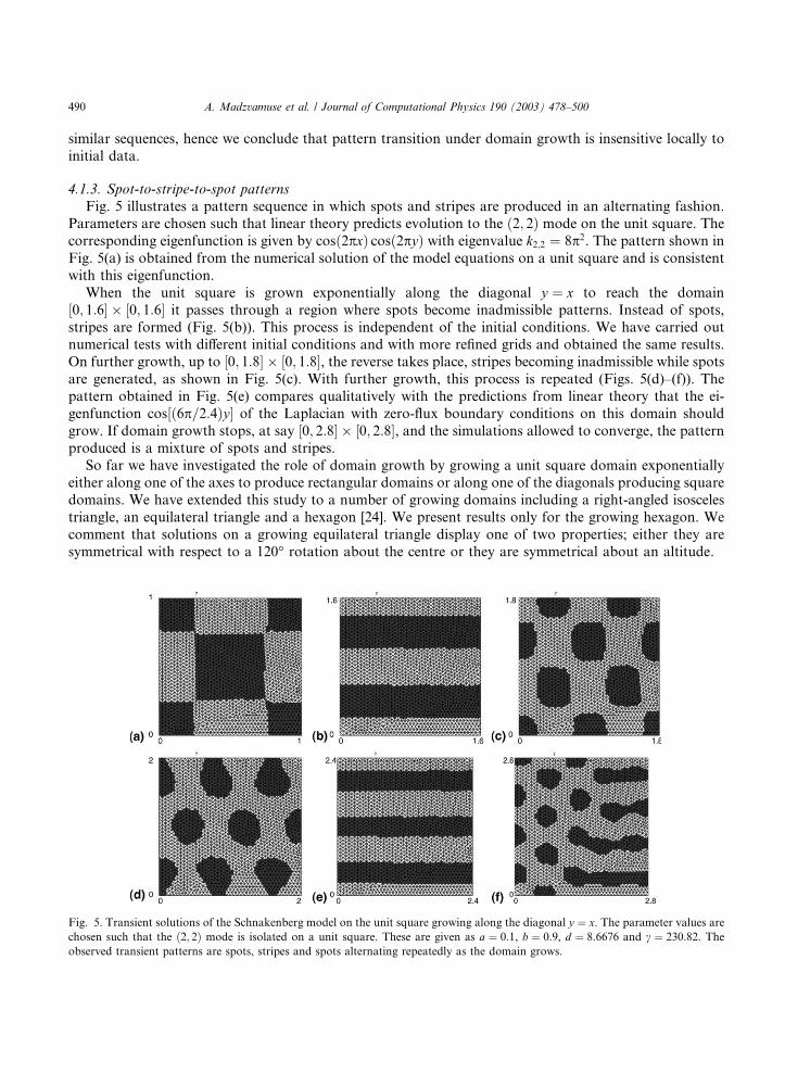
4.1.3. Spot-to-stripe-to-spot patterns

Fig. 5 illustrates a pattern sequence in which spots and stripes are produced in an alternating fashion.

Parameters are chosen such that linear theory predicts evolution to the ð2; 2Þ mode on the unit square. The

corresponding eigenfunction is given by cosð2pxÞ cosð2pyÞ with eigenvalue k2;2 ¼ 8p2. The pattern shown in

Fig. 5(a) is obtained from the numerical solution of the model equations on a unit square and is consistent

with this eigenfunction.

When the unit square is grown exponentially along the diagonal y ¼ x to reach the domain

½0; 1:6� � ½0; 1:6� it passes through a region where spots become inadmissible patterns. Instead of spots,

stripes are formed (Fig. 5(b)). This process is independent of the initial conditions. We have carried outnumerical tests with different initial conditions and with more refined grids and obtained the same results.

On further growth, up to ½0; 1:8� � ½0; 1:8�, the reverse takes place, stripes becoming inadmissible while spots

are generated, as shown in Fig. 5(c). With further growth, this process is repeated (Figs. 5(d)–(f)). The

pattern obtained in Fig. 5(e) compares qualitatively with the predictions from linear theory that the ei-

genfunction cos½ð6p=2:4Þy� of the Laplacian with zero-flux boundary conditions on this domain should

grow. If domain growth stops, at say ½0; 2:8� � ½0; 2:8�, and the simulations allowed to converge, the pattern

produced is a mixture of spots and stripes.

So far we have investigated the role of domain growth by growing a unit square domain exponentiallyeither along one of the axes to produce rectangular domains or along one of the diagonals producing square

domains. We have extended this study to a number of growing domains including a right-angled isosceles

triangle, an equilateral triangle and a hexagon [24]. We present results only for the growing hexagon. We

comment that solutions on a growing equilateral triangle display one of two properties; either they are

symmetrical with respect to a 120� rotation about the centre or they are symmetrical about an altitude.

Fig. 5. Transient solutions of the Schnakenberg model on the unit square growing along the diagonal y ¼ x. The parameter values are

chosen such that the ð2; 2Þ mode is isolated on a unit square. These are given as a ¼ 0:1, b ¼ 0:9, d ¼ 8:6676 and c ¼ 230:82. The

observed transient patterns are spots, stripes and spots alternating repeatedly as the domain grows.


4.1.4. Transient patterns on a hexagon

We investigate the role of domain growth on a hexagon of unit side given by the vertices (1, 0); (12;ffiffi3

p

2);

(� 12;ffiffi3

p

2); (�1; 0); (� 1

2;�

ffiffi3

p

2) and (1

2;�

ffiffi3

p

2). The hexagon is allowed to grow exponentially from its centre to

three times its original size. Fig. 6 shows the corresponding numerical solutions of the model system with

homogeneous Neumann boundary conditions. The parameter values are unchanged from those used on the

equilateral triangle.

Fig. 6. Typical numerically computed patterns on a growing hexagon for the Schnakenberg model with parameter values a ¼ 0:1,

b ¼ 0:9, d ¼ 10 and c ¼ 114. Stripe, spot and circular patterns are exhibited. Circular patterns become pronounced as the hexagon

grows in size. As the domain reaches its maximum size, the system evolves to an inhomogeneous steady-state solution consisting of

stripes and spots.

Fig. 7. (a) The 16-sided polygonal approximation to the butterfly wing of Papilio dardanus. (b) A typical sequence of the polygons

generated by the cubic spline interpolation at selected time intervals. The spring analogy is used to deform and move the mesh

generated in wing 1 given successive locations of the deforming boundary using cubic splines.



Initially we observe stripes (Fig. 6(a)) evolving to spots as the domain grows as shown in Fig. 6(b). These

spots further evolve to stripes (Figs. 6(c) and (d)). A mixed mode solution then gives rise to circular patterns

as illustrated in the sequence shown in Figs. 6(e)–(k). The circular patterns continue to evolve as the domain

deforms continuously until it reaches its final size. On this fixed domain the spatially inhomogeneous

steady-state pattern obtained is that of stripes and spots combined (Fig. 6(l)). The sequence illustrated is

independent of the initial conditions.

Although this sequence exhibits several features in common with our previous simulations above, a new

pattern is observed, namely circular patterns. The appearance of such patterns seems to be due to the natureof the geometry. The circular patterns appear as transient solutions when stripes and spots occur at almost

the same time but neither solution dominates due to domain growth. Such patterns have been observed in

zebrafish [37] and Pomacanthus [22]. This phenomenon could explain the emergence of circular patterns of

pigmentation on fish which takes place as the fish grows in size. A combination of spots and stripes are

observed when the zebrafish attains its maximum size, which compares qualitatively with the inhomoge-

neous steady-state pattern computed on the final fixed domain. When the domain reaches its final size the

numerical solution converges to a mixed pattern of stripes and spots (Fig. 6(l)). The evolution of the

transient solutions on the growing domain is insensitive to the initial conditions. Therefore under domaingrowth the model is robust as the patterns generated are independent of the initial conditions, when these

are small amplitude perturbations about the uniform steady state.

4.2. Transient solutions on irregular domains: Gierer–Meinhardt kinetics

The aim of this section is to illustrate the generality of our numerical technique in dealing with arbitrary

simply connected domains. This work was motivated by the study of growth colour patterns in the butterfly

wing Papilio dardanus. The biological background to the mathematical problem is well documented in the

papers by Sekimura et al. [43–45] and in the book by Nijhout [34]. Our aim here is not to compute patterns

typically observed in biological experiments but to illustrate the generality of our numerical method.

The problem here is, given a discrete sequence of the wing size and shape of the butterfly P. dardanus can

we predict and calculate the evolving patterning process? Typically the discrete sequence is given by thescans at the following time intervals, 12, 36, 48, 60, 72 and 96 h (Fig. 7 and Table 1). Interpolation between

Table 1

The boundary coordinates of the 16-sided polygonal domain of the six wings in Fig. 7a

Time (s) 0:432 � 105 1:296 � 105 1:728 � 105 2:16 � 105 2:59 � 105 3:456 � 105

ðxs1 ; ys1 Þ ð�0:43;�0:39Þ ð�1:02;�0:13Þ ð�1:04;�0:59Þ ð�1:3;�0:87Þ ð�1:52;�0:65Þ ð�1:96;�0:65Þðxs2 ; ys2 Þ ð�0:26;�0:65Þ ð�0:87;�0:5Þ ð�0:65;�1:02Þ ð�0:74;�1:52Þ ð�0:65;�1:65Þ ð�1:35;�1:3Þðxs3 ; ys3 Þ ð�0:13;�0:91Þ ð�0:2;�1:02Þ ð�0:22;�1:26Þ ð�0:22;�1:7Þ ð�0:22;�1:78Þ ð�0:74;�2:04Þðxs4 ; ys4 Þ ð0:09;�1:0Þ ð0:22;�1:09Þ ð0:22;�1:24Þ ð0:43;�1:61Þ ð0:65;�1:61Þ ð0:43;�2:04Þðxs5 ; ys5 Þ ð0:3;�0:96Þ ð0:43;�1:0Þ ð0:52;�1:04Þ ð1:09;�1:11Þ ð1:22;�1:22Þ ð1:96;�1:3Þðxs6 ; ys6 Þ ð0:5;�0:8Þ ð1:04;�0:48Þ ð0:74;�0:91Þ ð1:39;�0:74Þ ð1:87;�0:57Þ ð2:17;�0:87Þðxs7 ; ys7 Þ ð0:74;�0:65Þ ð1:2;�0:22Þ ð1:17;�0:37Þ ð1:52;�0:35Þ ð2:04;�0:22Þ ð2:72;�0:07Þðxs8 ; ys8 Þ ð0:78;�0:57Þ ð1:3; 0:11Þ ð1:35;�0:09Þ ð1:67; 0:09Þ ð2:13; 0:63Þ ð2:7; 0:87Þðxs9 ; ys9 Þ ð0:79;�0:43Þ ð1:26; 0:5Þ ð1:3; 0:46Þ ð1:57; 1:17Þ ð2:15; 1:04Þ ð2:78; 1:74Þðxs10 ; ys10 Þ ð0:8;�0:09Þ ð1:24; 0:83Þ ð1:37; 0:8Þ ð1:43; 1:39Þ ð2:22; 1:3Þ ð2:61; 2:04Þðxs11 ; ys11 Þ ð0:65; 0:2Þ ð1:1; 0:98Þ ð1:3; 0:96Þ ð1:22; 1:43Þ ð2:09; 1:43Þ ð2:37; 2:09Þðxs12 ; ys12 Þ ð0:43; 0:43Þ ð0:76; 1:0Þ ð0:74; 1:04Þ ð0:87; 1:39Þ ð1:30; 1:52Þ ð1:13; 1:7Þðxs13 ; ys13 Þ ð0:22; 0:61Þ ð�0:22; 1:0Þ ð0:09; 1:2Þ ð0:33; 1:52Þ ð0:4; 1:54Þ ð0:67; 1:83Þðxs14 ; ys14 Þ ð0:0; 0:65Þ ð�0:83; 0:8Þ ð�0:65; 1:0Þ ð�0:3; 1:52Þ ð�0:37; 1:61Þ ð�0:65; 1:74Þðxs15 ; ys15 Þ ð�0:13; 0:59Þ ð�0:87; 0:59Þ ð�0:96; 0:72Þ ð�0:87; 1:3Þ ð�1:13; 1:35Þ ð�1:22; 1:57Þðxs16 ; ys16 Þ ð�0:43; 0:26Þ ð�1:02; 0:35Þ ð�1:04; 0:43Þ ð�1:3; 0:87Þ ð�1:52; 0:87Þ ð�1:96; 1:52ÞaHere, sk represents the successive locations of the (x; yÞ end points on each segment of the polygon.


the positions of the boundary nodes of the boundary shape is achieved with cubic splines thus defining a

continuously deforming domain. Once the boundary position of the continuously deforming boundary is

located, the spring analogy is applied at each time step to define the internal mesh and hence to define the

motion on the internal nodes.

We solve the Gierer–Meinhardt reaction kinetics with homogeneous Neumann boundary conditions

for both u and v. We note that these are not realistic boundary conditions for the butterfly pattern [45].

Initial conditions are taken as random perturbations about a constant value. Figs. 8 and 9 show the

results of such computations. As the domain grows continuously transient patterns evolve from spots tocircular patterns. The scale changes in Figs. 8 and 9 are small compared to the rest of the previous figures.

Therefore we plot the figures on the same scale ½�2; 2:6� � ½�2; 2� and this is not shown in the illustrated

figures.

Fig. 8. Transient patterns of the solution u corresponding to the Gierer–Meinhardt reaction model with parameter values a ¼ 0:1,

b ¼ 1:0, K ¼ 0:5, d ¼ 70:8473 and c ¼ 619:45. Spot patterns continue to evolve with domain growth. The numerical simulations are

carried out on a typical mesh of 4730 elements with 2466 nodes.

Fig. 9. Fig. 8 continued. As the domain continuously deforms, a combination of stripes and spots is exhibited on the same

domain.


5. Conclusion and discussion

The novel application of the moving grid finite element method to reaction–diffusion systems on a

continuously deforming domain has opened new avenues in the study of pattern formation and transition

in Biology. In particular, we have developed a freely available software package that can be used not only

to investigate pattern formation, but also to predict pattern transition. All results reported in this paper are

produced with this package and it can be downloaded from: http://web.comlab.ox.ac.uk/oucl/work/an-

dy.wathen/software.html.This technique has been applied to the study of colour pattern formation of the butterfly wing

P. dardanus [25,26,45], and growth patterns in bivalve ligaments [25,26,48].




We have observed that stripes can evolve into stripes, spots into spots and sometimes stripes evolve into

spots which in turn involve into circular patterns. The emergence of such exotic patterns is due to domain

growth. Domain growth appears to enhance robustness in pattern selection and transition: lack of ro-

bustness has been one of the main criticisms of the Turing theory of pattern formation on fixed domains.

The generality of our numerical method allows us to carry out further investigative real studies into

pattern transition in biological problems. Currently we are investigating growth patterns of the butterfly

wing P. dardanus and of the zebrafish.

Acknowledgements

This work (AM) was supported by a grant from EPSRC Life Sciences Initiative (GR/R03914). PKM

was partly supported by a Royal Society Leverhulme Trust Senior Fellowship. We thank Professor Toshio

Sekimura (Chubu University, Japan) for bringing the problem of butterfly pigmentation patterning to our

attention and for providing the data used in Fig. 7.

Appendix A. Linear analysis

Standard linear stability analysis shows that diffusion-driven instability of a uniform steady state of the

systems (2.2)–(2.8) occurs if the following conditions hold (see, for example, the books by [16,33]:

fu þ gv < 0; ðA:1Þ

fugv � fvgu > 0; ðA:2Þ

dfu þ gv > 0; ðA:3Þ

ðdfu þ gvÞ2 � 4dðfugv � fvguÞ > 0; ðA:4Þ

where the partial derivatives are evaluated at the steady state. Inequalities (A.1)–(A.4) define a domain of

parameter space, known as the Turing space, wherein the uniform steady state is unstable to random small

perturbations.

Under these conditions, spatial disturbances with wavenumbers k 2 ðk�; kþÞ will initially grow, where

k2� ¼ cðdfu þ gvÞ �

ffiffiffiffiffiffiffiffiffiffiffiffiffiffiffiffiffiffiffiffiffiffiffiffiffiffiffiffiffiffiffiffiffiffiffiffiffiffiffiffiffiffiffiffiffiffiffiffiffiffiffiffiffiffiffiffiffiffiðdfu þ gvÞ2 � 4dðfugv � fvguÞ

q2d

: ðA:5Þ

In the case we are interested in, namely, the unit square with zero flux boundary conditions, a furtherrestriction on k is that it must take discrete values p

ffiffiffiffiffiffiffiffiffiffiffiffiffiffiffiffim2 þ n2

p, corresponding to the spatial mode

cosmpx cos npy denoted by ðm; nÞ.For diffusion-driven instability to occur we require that the Turing conditions (A.1)–(A.4) are satisfied

and if we wish to isolate a certain mode, say ðm; nÞ, then

k2max 6 k2� < k2m;n ¼ p2ðm2 þ n2Þ < k2þ 6 k2min; ðA:6Þ

where

k2max ¼ maxf8k2p;q : k2p;q < k2m;n for some p; qg; ðA:7Þ

Table 2

Values for d and c under which a particular mode is isolated on a unit square domain for the Gierer–Meinhardt, Thomas and

Schnakenberg models

Mode ðm; nÞ Gierer–Meinhardt Thomas Schnakenberg

d c d c d c

(1,0) 520.1573 67 427.0152 44 10 29

(1,1) 105.1573 168.8 39.0152 79 11.5776 70.6

(2,0) 84.1573 238.26 54.0152 122 10 114

(2,1) 77.6473 411.42 29.0152 170 9.1676 176.72

(2,2) 75.1573 483.43 30.9152 252 8.6676 230.82

(3,0) 70.8473 619.45 36.0152 269 8.6176 265.22

(3,1) 72.1573 756.23 27.5152 320 8.6676 329.20

(3,2) 73.1573 901.38 28.4152 402 8.8676 379.21

(3,3) 70.5573 1266.99 28.5152 553 8.6076 535.09

(4,0) 71.1573 1033.51 31.5152 473 8.6676 435.99

(4,1) 70.3573 1164.86 27.0252 506 8.5876 492.28

(4,2) 71.1573 1519.87 27.0252 596 8.7176 625.35

(4,3) 71.1573 1580.66 27.0252 745 8.6676 666.82

(4,4) 73.1473 2167 27.0252 953 8.6076 909.66


k2min ¼ minf8k2p;q : k2p;q > k2m;n for some p; qg: ðA:8Þ

We impose the lower k2max and upper k2min bounds on k2� and k2þ respectively so that k2m;n will be the only

eigenvalue with a positive real part. We wish to isolate a certain mode, that is, we want linear stability

analysis to predict that the uniform steady state goes unstable only to spatial perturbations cosmpx cos npywith a particular ðm; nÞ. Table 2 shows the parameter values d and c for some fixed parameter values:

1. Gierer–Meinhardt model: a ¼ 0:1, b ¼ 1:0, k ¼ 0:5;2. Thomas model: a ¼ 150, b ¼ 100, K ¼ 0:05, a ¼ 1:5 q ¼ 13;

3. Schnakenberg model: a ¼ 0:1 and b ¼ 0:9.

Appendix B. Cubic spline interpolation

The basic idea of a cubic spline interpolation is that given a tabulated function, xi ¼ xiðtiÞ; yi ¼ yiðtiÞ,i ¼ 1; . . . ; n, we determine the intermediate values of ðx; yÞ of the function say between frame 1 and 2, that is

at time 12 and 18 h, every 15 s. n is the number of frames. For illustrative purposes, let us consider the time

interval ti and tiþ1, i ¼ 1; . . . ; n� 1. The aim is to obtain an interpolation formula that is smooth in the firstderivative and continuous in the second derivative, both within an interval and at its boundaries. The

interpolation can be shown to be of the form

ðx; yÞ ¼ C0 ðxj; yjÞ þ C1 ðxjþ1; yjþ1Þ þ C2 ðx00j ; y00j Þ þ C3 ðx00jþ1; y00jþ1Þ ðB:1Þ

with j ¼ 1; . . . ; nbry, nbry is the number of boundary grid coordinates. 00 denotes the second derivative withrespect to time, and

C0 ¼tjþ1 � ttjþ1 � tj

; C1 ¼ 1� C0 ¼t � tj

tjþ1 � tj; C2 ¼

1

6ðC3

0 � C0Þðtjþ1 � tjÞ2; C3 ¼1

6ðC3

0 � C0Þðtjþ1 � tjÞ2:

Now, the assumption of continuity of the first derivative across the boundary between any two intervals,

gives rise to the system of equations


tj � tj�1

6ðx00j�1; y

00j�1Þ þ

tjþ1 � tj�1

3ðx00j ; y00j Þ þ

tjþ1 � tj6

ðx00jþ1; y00jþ1Þ

¼ ðxjþ1; yjþ1Þ � ðxj; yjÞtjþ1 � tj

� ðxj; yjÞ � ðxj�1; yj�1Þtj � tj�1

: ðB:2Þ

In our case uniqueness is guaranteed by setting both the second derivatives of ðx; yÞ at the end points equal

to zero, giving the so-called natural cubic spline. Eq. (B.2) is tridiagonal, which is a huge practical ad-

vantage. Therefore the system of equations are solved in OðNÞ operations by the tridiagonal algorithm.

Once the ðX;YÞ boundary coordinates are obtained through the cubic spline interpolation, we apply the

spring analogy to calculate and move the new interior coordinates from the old coordinates.

B.1. Mesh movement using the spring analogy

The spring analogy is a common technique of deforming a mesh [10]. It consists of replacing the mesh by

fictitious springs. There are two types of springs, the vertex and the segment spring analogies. The vertex

spring is used mainly to refine a particular mesh, while the segment spring is appropriate for deforming and

moving a given mesh. In both cases, the segments are considered as springs. The springs are linear and

Hooke�s law is applied to determine the displacements of the nodes. For the segment springs, the equi-

librium lengths of the springs are equal to the initial lengths of the segments. The force at each node i, say, isdetermined by

Fi ¼Xnij¼1

aijðdj � diÞ: ðB:3Þ

Here, di is the displacement of node i, ni is the total number of nodes surrounding node i. aij is the spring

stiffness which according to Batima [9], is given by aij ¼ 1=ffiffiffiffiffiffiffiffiffiffiffiffiffiffiffiffiffiffiffiffiffiffiffiffiffiffiffiffiffiffiffiffiffiffiffiffiffiffiffiffiffiffiðxi � xjÞ2 þ ðyi � yjÞ2

q. At static equilibrium, Fi

is zero, and applying Dirichlet boundary conditions, we obtain a system of linear algebraic equations whose

unknowns are new displacements. The nodal displacements are therefore calculated as xnewi ¼ xold

i þ dfinali .Observe that the system

Oi ¼Xnij¼1

aijðdj � diÞ ðB:4Þ

is symmetric and positive definite. The resultant matrix on the left-hand side for the unknown displace-

ments is an M-matrix. When a boundary is moved or deformed, the boundary nodal positions are strongly

imposed by Dirichlet boundary conditions. The system is solved by a preconditioned Conjugate Gradient

method where the preconditioner is determined by an incomplete Cholesky factorisation [39].

References

[1] R.A. Adams, Sobolev Spaces, Academic Press, New York, 1975.

[2] J.L. Arag�oon, C. Varea, R.A. Barrio, P.K. Maini, Spatial patterning in modified turing systems: application to pigmentation

patterns on Marine fish, Forma 13 (1998) 213–221.

[3] J.L. Arag�oon, M. Torres, D. Gil, R.A. Barrio, P.K. Maini, Turing patterns with pentagonal symmetry, Phys. Rev. E 65 (2002) 1–9.

[4] M.J. Baines, Moving finite elements, Monographs on Numerical Analysis, Clarendon Press, Oxford, 1994.

[5] M.J. Baines, A.J. Wathen, Moving finite element methods for evolutionary problems. I. Theory, J. Comp. Phys. 79 (1988) 245–

269.

[6] Y.I. Balkarei, A.V. Grigo€rrYants, Y.A. Rhzanov, M.I. Elinson, Regenerative oscillations, spatial-temporal single pulses and static

inhomogeneous structures in optically bistable semiconductors, Opt. Commun. 66 (1988) 161–166.


[7] R.A. Barrio, C. Varea, J.L. Arag�oon, P.K. Maini, A two-dimensional numerical study of spatial pattern formation in interacting

systems, Bull. Math. Biol. 61 (1999) 483–505.

[8] R.A. Barrio, P.K. Maini, J.L. Arag�oon, M. Torres, Size-dependent symmetry breaking in models for morphogenisis, Physica D

2920 (2002) 1–12.

[9] J.T. Batima, Unsteady Euler airfoil solutions using unstructured dynamic meshes, AIAA J. 28 (8) (1990) 1381–1388.

[10] J.F. Blom, Considerations of the spring analogy, Int. J. Numer. Meth. Fluids 12 (2000) 647–668.

[11] S.C. Brenner, L.R. Scott, The Mathematical Theory of Finite Element Methods, Springer, Berlin, 1994.

[12] N.N. Carlson, K. Miller, Design and application of a gradient-weighted moving finite element code I: in one dimension, SIAM J.

Sci. Comput. 19 (3) (1998) 728–765.

[13] N.N. Carlson, K. Miller, Design and application of a gradient-weighted moving finite element code II: in two dimensions, SIAM

J. Sci. Comput. 19 (3) (1998) 766–798.

[14] E.J. Crampin, Reaction–diffusion patterns on growing domains, D. Phil. Thesis, University of Oxford, 2000.

[15] E.J. Crampin, E.A. Gaffney, P.K. Maini, Reaction and diffusion on growing domains: scenarios for robust pattern formation,

Bull. Math. Biol. 61 (2002) 1093–1120.

[16] L. Edelstein-Keshet, Mathematical Models in Biology, Random House, New York, 1988.

[17] P. Gray, S.K. Scott, Autocatalytic reactions in the isothermal, continuous stirred tank reactor: isolas and other forms of

multistability, Chem. Eng. Sci. 38 (1) (1983) 29–43.

[18] P. Gray, S.K. Scott, Autocatalytic reactions in the isothermal, continuous stirred tank reactor: oscillations and the instabilities in

the system Aþ 2B ! 3B, B ! C, Chem. Eng. Sci. 39 (6) (1984) 1087–1097.

[19] A. Gierer, H. Meinhardt, A theory of biological pattern formation, Kybernetik 12 (1972) 30–39.

[20] P.K. Jimack, A.J. Wathen, Temporal derivatives in the finite element method on continuously deforming grids, SIAM J. Numer.

Anal. 28 (4) (1991) 990–1003.

[21] C. Johnson, Numerical Solution of Partial Differential Equations by the Finite Element Method, Cambridge University Press,

Cambridge, MA, 1987.

[22] S. Kondo, R. Asai, A reaction–diffusion wave on the skin of the marine angelfish Pomacanthus, Nature 376 (1995) 765–768.

[23] V.I. Krinsky, Self-organisation, Auto-Waves and Structures Far From Equilibrium, Springer, Berlin, 1984.

[24] A. Madzvamuse, A numerical approach to the study of spatial pattern formation, D. Phil. Thesis, University of Oxford, 2000.

[25] A. Madzvamuse, P.K. Maini, A.J. Wathen, T. Sekimura, A predictive model for color pattern formation in the butterfly wing of

Papilio dardanus, Hiroshima Math. J. 32 (2002) 325–336.

[26] A. Madzvamuse, R.D.K. Thomas, P.K. Maini, A.J. Wathen, A numerical approach to the study of spatial pattern formation in

the Ligaments of Arcoid Bivalves, Bull. Math. Biol. 64 (2002) 501–530.

[27] P.K. Maini, M. Solursh, Cellular mechanisms of pattern formation in the development of limb, Int. Rev. Cytol. 129 (1991) 91–133.

[28] H. Meinhardt, The Algorithmic Beauty of Sea Shells, Springer, Heidelberg, New York, 1995.

[29] K. Miller, R.N. Miller, Moving finite elements. Part I, SIAM J. Numer. Anal. 18 (1981) 1019–1032.

[30] K. Miller, Moving finite elements. Part II, SIAM J. Numer. Anal. 18 (1981) 1033–1057.

[31] J.D. M€uuller, P.L. Roe, H. Deconinck, A frontal approach for internal node generation for Delaunay triangulation, Int. J. Numer.

Methods Fluids 17 (3) (1993) 241–256.

[32] J.D. Murray, On pattern formation mechanisms for lepidopteran wing patterns and mammalian coat markings, Philos. Trans.

Roy. Soc. London B 295 (1981) 473–496.

[33] J.D. Murray, Mathematical Biology, Springer, Heidelberg, New York, 1993.

[34] H.F. Nijhout, A comprehensive model for colour pattern formation in butterflies, Proc. Roy. Soc. London B 239 (1990) 81–113.

[35] T. Nozakura, S. Ikeuchi, Formation of dissipative structures in galaxies, Astrophys. J. 279 (1984) 40–52.

[36] K.J. Painter, Chemotaxis as a mechanism for morhogenesis, D. Phil. Thesis, University of Oxford, 1997.

[37] K.J. Painter, P.K. Maini, H.G. Othmer, Stripe formation in juvenile Pomacanthus explained by a generalised Turing mechanism

with chemotaxis, Proc. Natl. Acad. Sci. USA 96 (1999) 5549–5554.

[38] T.N. Reddy, An Introduction to the Finite Element Method, McGraw-Hill, New York, 1984.

[39] Y. Saad, SPARSEKIT, a basic tool kit for sparse matrix computations, 1994, http://www-users.cs.umn.edu/ saad/.

[40] Y. Saad, Iterative Methods for Sparse Linear Systems, PWS Publishing, 1996.

[41] J. Schnakenberg, Simple chemical reaction systems with limit cycle behavior, J. Theoret. Biol. 81 (1979) 389–400.

[42] L.A. Segel, J.L. Jackson, Dissipative structure: an explanation and an ecological example, J. Theoret. Biol. 37 (1972) 545–

559.

[43] T. Sekimura, P.K. Maini, J.B. Nardi, M. Zhu, J.D. Murray, Pattern formation in lepidopteran wings, Comm. Theoret. Biol. 5 (2–

4) (1998) 69–87.

[44] T. Sekimura, M. Zhu, J. Cook, P.K. Maini, J.D. Murray, Pattern formation of scale cells in lepidoptera by differential origin-

dependent cell adhesion, Bull. Math. Biol. 61 (1999) 807–827.

[45] T. Sekimura, A. Madzvamuse, A.J. Wathen, P.K. Maini, A model for colour pattern formation in the butterfly wing of Papilio

dardanus, Proc. Roy. Soc. London B 267 (2000) 851–859.

http://www-users.cs.umn.edu/saad/


[46] W. Sun, T. Tang, J.M. Ward, J. Wei, Numerical challenges for resolving spike dynamics for two reaction–diffusion systems, Stud.

Appl. Math. III (2003) 41–84.

[47] D. Thomas, Artificial enzyme membrane, transport, memory and oscillatory phenomena, in: D. Thomas, J.-P. Kervenez (Eds.),

Analysis and Control of Immobilised Enzyme Systems, Springer, Berlin, Heidelberg, New York, 1975, pp. 115–150.

[48] R.D.K. Thomas, A. Madzvamuse, P.K. Maini, A.J. Wathen, Growth patterns of noetiid ligaments: implications of developmental

models for the origin of an evolutionary novelty among arcoid bivalves, in: E.M. Harper, J.D. Taylor, J.A. Crame (Eds.), The

Evolutionary Biology of the Bivalvia, vol. 177, Geological Society Special Publication, 2000, pp. 279–289.

[49] A.M. Turing, The chemical basis of morphogenesis, Philos. Trans. Roy. Soc. London B 237 (1952) 37–72.

[50] D.B. White, The planforms and onset of convection with a temperature dependent viscosity, J. Fluid Mech. 191 (1988) 247–286.

A moving grid finite element method applied to - Mathematical Institute

Documents