A Motion Planner for Maintaining Landmark Visibility with a Differential Drive Robot

A Motion Planner for Maintaining LandmarkVisibility with a Differential Drive Robot

Jean-Bernard Hayet1, Claudia Esteves2, and Rafael Murrieta-Cid1∗

1 Centro de Investigacion en Matematicas, CIMAT. Guanajuato, Mexico.2 Facultad de Matematicas de la Universidad de Guanajuato. Guanajuato, Mexico.{jbhayet, cesteves, murrieta}@cimat.mx

Summary. This work studies the interaction of the nonholonomic and visibil-ity constraints of a robot that has to maintain visibility of a static landmark.The robot is a differential drive system and has a sensor with limited field ofview. We determine the necessary and sufficient conditions for the existenceof a path for our system to be able to maintain landmark visibility in thepresence of obstacles. We present a complete motion planner that solves thisproblem based on a recursive subdivision of a path computed for a holonomicrobot with the same visibility constraints.

1 Introduction

Landmarks are of common use in robotics, either to localize the robot withrespect to them [19] or to navigate in all kinds of environments [14, 4], beingused as goals or sub-goals to reach or perceive during the motion. Landmarkscan be defined in several manners: From single, characteristic image pointswith useful properties [17], up to a 3D object associated with a semantic labeland having 3D position accuracy [7]. In all cases, this definition involves atsome degree properties of saliency and invariance to viewpoint changes.

To use landmarks in the context of mobile robotics, the first basic require-ment is to perceive them during the robot motion. It is to this end that ourcurrent research efforts are focused on. Although landmarks have been exten-sively used, this is to our knowledge the first attempt to show whether or nota path of a holonomic robot in the presence of obstacles that has to maintainvisibility of one landmark with a limited sensor can be transformed into a fea-sible path for a differential drive robot (DDR). We believe that our researchis very pertinent given that a lot of mobile robots are DDRs equipped withlimited field of view sensors (e.g., lasers or cameras).

∗ This research was partially funded by CONACyT project 56754-F1 andCONCYTEG project 07-02-K662-097.

2 Jean-Bernard Hayet, Claudia Esteves, and Rafael Murrieta-Cid

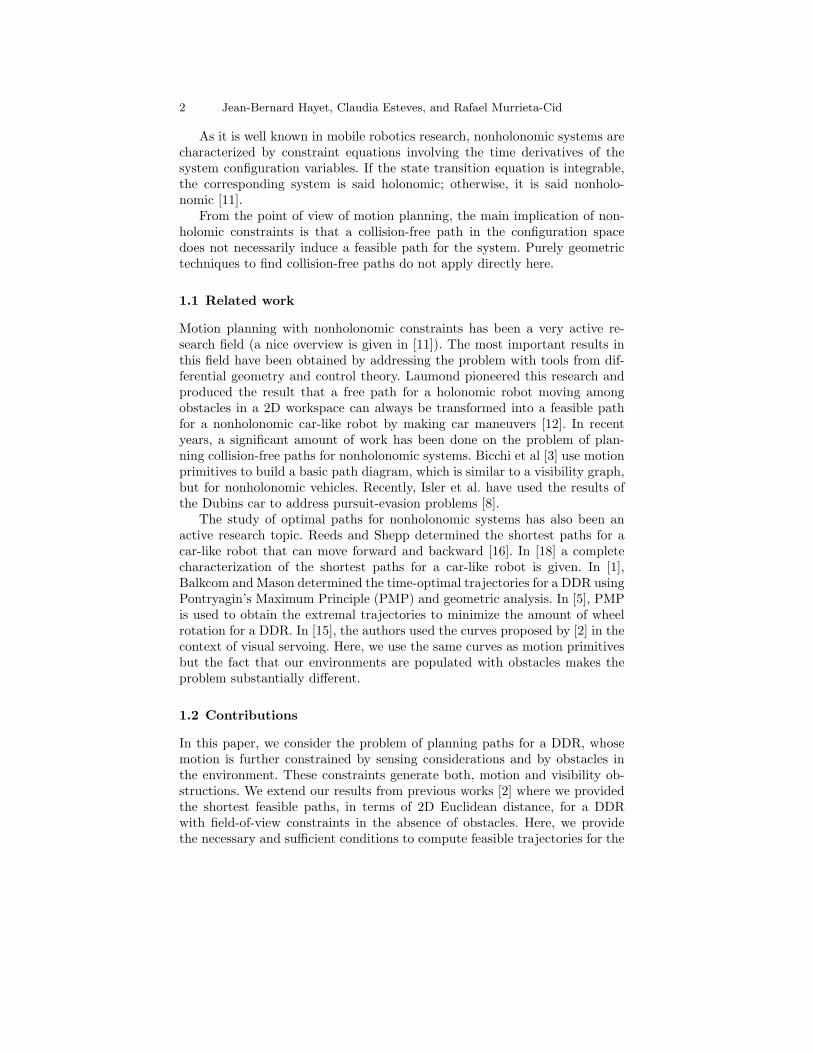
As it is well known in mobile robotics research, nonholonomic systems arecharacterized by constraint equations involving the time derivatives of thesystem configuration variables. If the state transition equation is integrable,the corresponding system is said holonomic; otherwise, it is said nonholo-nomic [11].

From the point of view of motion planning, the main implication of non-holomic constraints is that a collision-free path in the configuration spacedoes not necessarily induce a feasible path for the system. Purely geometrictechniques to find collision-free paths do not apply directly here.

1.1 Related work

Motion planning with nonholonomic constraints has been a very active re-search field (a nice overview is given in [11]). The most important results inthis field have been obtained by addressing the problem with tools from dif-ferential geometry and control theory. Laumond pioneered this research andproduced the result that a free path for a holonomic robot moving amongobstacles in a 2D workspace can always be transformed into a feasible pathfor a nonholonomic car-like robot by making car maneuvers [12]. In recentyears, a significant amount of work has been done on the problem of plan-ning collision-free paths for nonholonomic systems. Bicchi et al [3] use motionprimitives to build a basic path diagram, which is similar to a visibility graph,but for nonholonomic vehicles. Recently, Isler et al. have used the results ofthe Dubins car to address pursuit-evasion problems [8].

The study of optimal paths for nonholonomic systems has also been anactive research topic. Reeds and Shepp determined the shortest paths for acar-like robot that can move forward and backward [16]. In [18] a completecharacterization of the shortest paths for a car-like robot is given. In [1],Balkcom and Mason determined the time-optimal trajectories for a DDR usingPontryagin’s Maximum Principle (PMP) and geometric analysis. In [5], PMPis used to obtain the extremal trajectories to minimize the amount of wheelrotation for a DDR. In [15], the authors used the curves proposed by [2] in thecontext of visual servoing. Here, we use the same curves as motion primitivesbut the fact that our environments are populated with obstacles makes theproblem substantially different.

1.2 Contributions

In this paper, we consider the problem of planning paths for a DDR, whosemotion is further constrained by sensing considerations and by obstacles inthe environment. These constraints generate both, motion and visibility ob-structions. We extend our results from previous works [2] where we providedthe shortest feasible paths, in terms of 2D Euclidean distance, for a DDRwith field-of-view constraints in the absence of obstacles. Here, we providethe necessary and sufficient conditions to compute feasible trajectories for the

A Motion Planner for Maintaining Landmark Visibility 3

DDR with limited sensing capabilities to maintain landmark visibility in thepresence of obstacles. Our contributions in this work are:

1. We study the effect of limited range (min. and max.) over the optimalmotion primitives presented in [2] and show conditions such that theseoptimal primitives remain under both range and angular constraints.

2. We propose a complete planner to compute collision-free paths for a cir-cular holonomic robot maintaining landmark visibility among obstacles.

3. We provide the controls for the execution of the optimal motion primitives.4. We give the necessary and sufficient conditions for the feasibility of a path

for the DDR in the presence of obstacles and with visibility constraints,provided that a collision-free path generated for the holonomic systemwith the same visibility constraints exists.

5. We implement a complete motion planner for the DDR maintaining land-mark visibility, based on a recursive subdivision of the holonomic path.

2 Problem settings and approach overview

2.1 The differential drive robot

The DDR is described in Fig. 1(a). It is controlled through commands toits two wheels, i.e. through angular velocities wl and wr. Parameters for thiskind of robots are (1) the distance D from the axis center to each wheel and(2) the radius R of the wheels. Without loss of generality we suppose, in theremaining of this work, that these two quantities are unitary: D = R = 1.

We make the usual assignment of a body-attached x′y′ frame to the robot.The origin is at the midpoint between the two wheels, y′-axis parallel to theaxle, and the x′-axis pointing forward, parallel to the robot heading. The angleθ is the angle formed by the world x-axis and the robot x′-axis. The robotcan move forward and backward. The heading is defined as the direction inwhich the robot moves, so the heading angle with respect to the robot x-axisis zero (forward move) or π (backward move). The position of the robot w.r.tthe origin will be defined either in terms of Cartesian coordinates (x, y) or interms of polar coordinates (r, α) : r =

√x2 + y2, α = arctan y

x . Figure 1(a)sums up these conventions.

The robot is equipped with a pan-controllable sensor with limited field ofview (e.g., a camera), that can move w.r.t. the robot basis. We will supposethat this sensor is placed on the robot so that the optical center always liesdirectly above the origin of the robot’s local coordinate frame, i.e., the centerof rotation of the sensor is the same as the one of the robot. Its pan angle φis the angle from the robot x′-axis to its optical axis. The sensor is limited,both in angle and in range: φ ∈ [φ1, φ2] and the robot visibility region is madeby the points p such that the Euclidean distance d from p to the robot satisfydmin ≤ d ≤ dmax. We first assume that the robot moves in the free space(without physical obstacles), and then remove this assumption in Section 3.


θ

y′

dmax

dmin

D

ωr

ωl

rα

φ

x′Ox

y

(a)

SSL

L

LS

LSIO

P

(b)Fig. 1. (a) DDR with visibility constraints. The robot visibility region is depictedin yellow (filled region). (b) Spatial distribution of the nature of the shortest pathsfor a given point P , considering the range constraints dmin ≤ r ≤ dmax.

2.2 Optimal curves under visibility constraints for a DDR

Throughout all this article, we will make use of the results established byBhattacharya in [2], that exhibit the shortest paths for a DDR under visibil-ity constraints. These results are illustrated by Fig. 1(b). Given a point P anda landmark located at the origin O, the plane can be partitioned into threetypes of regions, according to the nature of the shortest paths. Blue regions(labeled with an “L” ) are made of points that can be connected to P throughline segments; in yellow regions (with the label “LS”), shortest paths are com-bination of a line segment and a logarithmic spiral; in green regions (labeledwith “SS”), shortest paths are combination of two logarithmic spirals. Thesespirals delimit the green and yellow regions and correspond to motions whenthe sensor angle φ is saturated at φ1 or φ2, whereas the inner blue and yellowregions are separated by arcs of circles tangent to the two aforementionedspirals. More details can be found in [2].

As a first step, we partly extend the latter results to the case of limitedrange, i.e. restricting the position of the robot to avoid the inner and outerred circular regions of Fig. 1(b).

Lemma 1. Assuming rP ≥ dmine2π

tan φ2−tan φ1 , the shortest paths for DDRsunder angular and range constraints starting at some point P = (rP , π

2 ) arethe same ones as for angular constraints only.

Proof. Note, first, that the radius r(t) is strictly monotonous (either increasingor decreasing) along all the shortest paths aiming at yellow and blue regionsof Fig. 1(b), labeled “S” and “LS”. Consider any shortest path s(t) : [0, 1] →SE(2) found under the angular constraint alone on these regions. If the initialand final configurations P and Q do satisfy the range constraints (e.g., dmin ≤rP ≤ rQ ≤ dmax), no point on s(t) can break the range constraint. Indeed,r(t) defines an homeomorphism from [0, 1] to [rP , rQ].


The situation becomes difficult when we consider the shortest paths formedby two spirals (green region on Fig. 1(b)), as in that case, the radius firstdecreases, then increases, i.e. the minimal radius may be below dmin. Thismay lead to a more complex distribution of shortest paths. However, we canrestrict P so that the minimum of r(t) on all possible arrival points remainsabove dmin. This minimum is at the intersection I (see Fig. 1(b)) of the twospirals, and rI can be easily calculated as rP e

−2πtan φ2−tan φ1 . It follows that

rP ≥ dmine2π

tan φ2−tan φ1

is a sufficient condition to ensure that the shortest paths are the same aswith the angular constraints only. ut

2.3 Approach overview

In [12] it has been shown that a free path for a holonomic robot movingamong obstacles in a 2D workspace can always be transformed into a free pathfor a nonholonomic car-like robot. Three necessary and sufficient conditionsguarantee the existence of the path for the car-like robot in the presence ofobstacles, provided that a path for a holonomic robot exist.

1. The nonholonomic robot must be Small Time Local Controllable (STLC).2. The existence of obstacles forces the use of some given metric in the plane

to measure the robot clearance. Hence, the topology induced by the robotmotion primitives metric and the one induced by the metric measuringthe distance between the obstacles and the robot must be equivalent.

3. There must be ε > 0 clearance between the robot and the obstacles.

Here, we follow the same methodology presented in [12], that we appliedto a DDR equipped with a sensor with a limited range and field of view.

As recorded in 2.2, the optimal motion primitives are of three types inour problem: straight-line segments, rotations in site without translation andspirals, i.e. curves for which the camera pan angle is saturated.

The remaining of this work is organized as follows: In Section 3 we presenta complete motion planner for a holonomic disk, which generates collision-free paths while maintaining landmark visibility. In Section 4 we show theadmissible controls to generate our motion primitives with our state transitionequation (system model) and we prove the STLC of our system. In Section5 we use our motion primitives to determine lower and upper bounds of thepaths metric and we show that the topology of the robot motion primitivesmetric and the metric used to measure the distance between the obstacles andthe robot are equivalent. Section 6 presents a motion planner for the DDRable to maintain landmark visibility and simulation results. Finally in Section7 we present the conclusion and future work.


3 Configuration space induced by visibility constraints

3.1 Configuration space without obstacles

As mentioned above, our robot must maintain visibility of a landmark. Byvisibility we mean that a clear line of sight, lying within the minimal andmaximal bounds of the sensor rotation angle and range, can join the landmarkand the sensor. The landmark is static and coincident with the origin O of thecoordinate system. The visibility constraints imposed by the landmark can bewritten as

θ = α− φ + (2k + 1)π, k ∈ Z, (1)φ1 ≤ φ ≤ φ2, (2)

dmin ≤ r ≤ dmax. (3)

From these equations, we can describe precisely the robot admissible con-figuration space Cadm. The robot can be seen as living in the special euclideangroup SE(2), as from Eq. 1, φ is not really a degree of freedom. Moreover,Eq. 1 adds a constraint on x, y and θ, that it can be rewritten

φ1 ≤ −θ + arctan(y

x) + (2k + 1)π ≤ φ2 for some k ∈ Z. (4)

This means that the visibility constraint both in range and angle can betranslated into virtual obstacles in SE(2). From Eq. 4, it is straightforwardto deduce the admissible configuration space, which is SE(2) minus theseobstacles. Fig. 2 gives a representation of the virtual obstacle (there is actuallyonly one obstacle) in SE(2) for φ2 = −φ1 = π

2 (a) and φ2 = −φ1 = π3 (b), as

the hollow volume in SE(2). It is worth noting that the free space resultingfrom this visibility obstacle is made of one single, helical-shaped componentof SE(2), the helical free component being smaller while the authorized panrange is smaller. We call Cφ

adm the admissible configuration space resultingfrom the angular constraints 2 and 3.

As far as the range constraints of the inequalities 3 are concerned, theyintroduce two other virtual cylindrical obstacles which reduce the admissibleconfiguration space into Cr

adm. Finally the combination of these constraintsgives rise to the admissible configuration space :

Cadm = Cφadm ∩ Cr

adm.

A simpler characterization can be made in the (x, y, φ) space, instead ofthe classical (x, y, θ). These two representations are equivalent, since φ andθ are related by Equation 1, and so are the constraints equations, but theadmissible configuration space, as depicted on Fig. 3(a), is easier to handle,as the constraints over φ (inequalities 2) do not depend on x or y. As a result,in that case, Cφ

adm is simply the space between the two planes φ = φ1 and


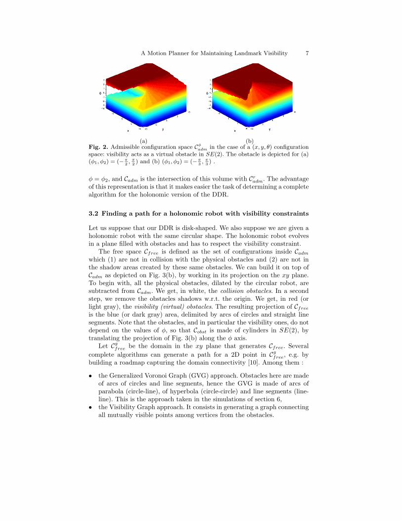
(a) (b)Fig. 2. Admissible configuration space Cφ

adm in the case of a (x, y, θ) configurationspace: visibility acts as a virtual obstacle in SE(2). The obstacle is depicted for (a)(φ1, φ2) = (−π

2, π

2) and (b) (φ1, φ2) = (−π

3, π

3) .

φ = φ2, and Cadm is the intersection of this volume with Cradm. The advantage

of this representation is that it makes easier the task of determining a completealgorithm for the holonomic version of the DDR.

3.2 Finding a path for a holonomic robot with visibility constraints

Let us suppose that our DDR is disk-shaped. We also suppose we are given aholonomic robot with the same circular shape. The holonomic robot evolvesin a plane filled with obstacles and has to respect the visibility constraint.

The free space Cfree is defined as the set of configurations inside Cadm

which (1) are not in collision with the physical obstacles and (2) are not inthe shadow areas created by these same obstacles. We can build it on top ofCadm as depicted on Fig. 3(b), by working in its projection on the xy plane.To begin with, all the physical obstacles, dilated by the circular robot, aresubtracted from Cadm. We get, in white, the collision obstacles. In a secondstep, we remove the obstacles shadows w.r.t. the origin. We get, in red (orlight gray), the visibility (virtual) obstacles. The resulting projection of Cfree

is the blue (or dark gray) area, delimited by arcs of circles and straight linesegments. Note that the obstacles, and in particular the visibility ones, do notdepend on the values of φ, so that Cobst is made of cylinders in SE(2), bytranslating the projection of Fig. 3(b) along the φ axis.

Let Cgfree be the domain in the xy plane that generates Cfree. Several

complete algorithms can generate a path for a 2D point in Cgfree, e.g. by

building a roadmap capturing the domain connectivity [10]. Among them :

• the Generalized Voronoi Graph (GVG) approach. Obstacles here are madeof arcs of circles and line segments, hence the GVG is made of arcs ofparabola (circle-line), of hyperbola (circle-circle) and line segments (line-line). This is the approach taken in the simulations of section 6,

• the Visibility Graph approach. It consists in generating a graph connectingall mutually visible points among vertices from the obstacles.


φ

φ

x

y

φ

1

2

(a) (b)

Fig. 3. (a) Cadm in the case of a (x, y, φ) configuration space. It is delimited by twohorizontal planes on φ and two vertical cylinders. (b) Construction of Cg

free with the(x, y, φ) representation for a circular robot reduced to a point in C (green): in the xyplane physical obstacles are dilated to define collision obstacles (in white) whereasshadows and visibility constraints define visibility obstacles (in red or light gray).

Any of these two approaches gives a complete algorithm for finding a pathfor a 2D point in Cg

free by connecting the desired start and end points to thegenerated graph [10]. By using this classical result, we can now state

Theorem 1. The problem of planning a path in Cfree ⊂ SE(2) for a holo-nomic, circular robot with visibility constraints on both range and angulardisplacement of its sensor is reductible to the problem of finding a path for asingle point in Cg

free ⊂ R2.

Proof. Let (xi, yi, θi)T and (xf , yf , θf )T be two free initial and final configura-tions in SE(2). By construction, the 2D points (xi, yi)T and (xf , yf )T belongto Cg

free. Now suppose that we can find a path sg connecting them in Cgfree,

sg : [0, 1] → Cgfree

sg(0) = (xi, yi)T , sg(1) = (xf , yf )T

sg(t) = (x(t), y(t))T .

Then, if φi and φf are the sensor angle relative to the robot (given byEq. 1) at initial and final configurations, let us define:

sθ : [0, 1] → SO(2)sθ(t) = arctan( y(t)

x(t) )− (1− t)φi − tφf + π.

The function sθ is continuous on [0, 1] since sg is also continuous and(x(t), y(t)) 6= (0, 0). Then we can define the following path in SE(2) :

s : [0, 1] → SE(2)s(t) = (x(t), y(t), sθ(t))T .

The path is continuous, it satisfies the initial and final constraints, and,by construction, as for all t ∈ [0, 1], (1 − t)φi + tφf ∈ [0, 2π), it also satisfiesthe visibility constraints at every point.


Conversely, if we are not able to find any free path in Cgfree, we cannot

have any free path in SE(2): if there were, its projection on R2 would also befree, which contradicts our initial assumption. As a consequence, an algorithmthat solves the planning problem in Cg

free also solves the problem in Cfree. ut

4 System controls and small time local controlability

We generate a state transition equation with two controls only. In this scheme,we suppose that the sensor is pointing to the landmark by adjusting its anglevalue according to equation 1, thus the sensor control is not considered inthis motion analysis. It must be determined, whether this system is STLCor not. Far enough from the visibility obstacles, the robot can move forwardand backward, hence it is a symmetric system. The construction of the statetransition equation is as follows.

First, we get the derivatives φ and α:

φ = α− θ and α =yx− xy

x2 + y2. (5)

The linear and angular velocities u1 and u2 can be expressed in functionof the wheels controls wl and wr, as:

u1 = wr + wl, u2 = wr − wl. (6)

Therefore, the state variables are:

θ = wr − wl, x = cos θ(wr + wl) and y = sin θ(wr + wl). (7)

A key observation is the following: φ is not a degree of freedom. It canbe expressed as a function of x, y and θ. Hence, the robot configuration istotally defined by (x, y, θ). φ and φ are adjusted so that the system maintainlandmark visibility.

The derivative φ can be expressed directly in function of the controls u1, u2

and the configuration variables (θ, x, y). This can be done by substituting in5, the values of α and θ from Equations 5 and 7,

φ =(y cos θ − x sin θ)u1

x2 + y2− u2. (8)

Therefore, the state transition equation takes the form: xy

θ

=

cos θ 0sin θ 0

0 1

(u1

u2

), (9)

which is exactly the same of the differential drive robot[1, 13].We underline that, the three only motion primitives are straight lines,

rotation in site and logarithmic spirals [2]. The vector field associated to the


straight line is −→X1 = (cos θ, sin θ, 0)T , the one associated to the rotation insite is simply −→X2 = (0, 0, 1)T .

Now let us express the vector field associated to the spirals. The equationsof these curves are [2]:

r = r0e(α0−α)/ tan φ, (10)

where (r0, α0) is one point of the spiral and φ remain constant along it.From the previous equation, and by using (1) the equation φ = α− θ + π and(2) the relation α = arctan y

x , we can easily derive the corresponding vectorfield, after some algebraic developments

−→X3 =

− x2+y2

y−x tan θ

− tan θ x2+y2

y−x tan θ

1

. (11)

This vector field is not defined for y = x tan θ, which corresponds to zoneswhere the robot has to follow a straight line. In fact, in that case −→X3 = −→

X1.A question that naturally arises is: What are the open-loop controls needed

for the robot to follow the logarithmic, saturating sensor pan angle? Thesecontrols can be derived from the following. When the robot moves drawingsector of logarithmic spirals, the camera pan angle is saturated and hencethe landmark is in the limit of the sensor field of view. Hence, the saturatedsensor pan angle, and more generally any trajectory maintaining the sensorpan angle constant, satisfy φ = 0.

Now, by using Eq.8, we obtain a relation between u1 and u2:

(y cos θ − x sin θ)u1 = (x2 + y2)u2,

which can be easily re-written in its polar form

u2 =1ru1 sin(α− θ). (12)

In terms of left and right wheels controls, we deduce from Eq.12, for r > 0,{wr = 1wl = r−sin(α−θ)

r+sin(α−θ) .

Again in terms of u1 and u2, and by setting u1 = 1,{u1 = 1u2 = sin(α−θ)

r .

Thus, make our system follow the optimal motion primitives, it is sufficientto consider three admissible pairs of controls (u1, u2) that allow to satisfy thevisibility constraint and lead the robot to trace these primitives: Straight lines,rotation in site and logarithmic spirals. These controls are respectively


(10

),

(01

)and

(1

sin(α−θ)r

). (13)

As shown above, the third control produces a logarithmic spiral, and cor-responds to a linear combination of the first two vector fields −→X1 and −→X2,

−→X3 = a1

−→X1 + a2

−→X2 where ai ∈ R. (14)

Hence, the state transition equation presented in 9 can be used to modelour system and trace our motion primitives, and therefore our system is STLCby using Chow theorem [11, 6, 13].

The Lie bracket operation computed over vector files −→X1 and −→

X2 is(sin θ,− cos θ, 0)T . It is immediate to see that this new vector field is lin-early independent from −→

X1 and −→X2. Hence, this system is small time locally

controllable everywhere in the open of the free space.Note that the first two controls are constant and therefore bounded, and

the third one is also bounded since we consider r > rmin > 0.

5 Analysis of the metric induced by shortest paths

The lengths along the shortest paths defined by Bhattacharya curves clearlyestablish a metric in Cg

free. Let us prove that this metric is locally equivalentto the Euclidean metric in R2. Let (xi, yi)T and (xf , yf )T be a pair of initialand final points in the free space. As recorded in 2.2 , there are just threekinds of shortest paths: a line segment (on which the length is obviouslyequal to the Euclidean distance in R2), a concatenation of line segment anda logarithmic spiral at saturated φ (Fig. 4, left) and a concatenation of twospirals at saturated φ (Fig. 4, right). Without loss of generality, we can analyzethe two cases depicted in Fig. 4, corresponding to zones II and V in [2].

Pf

Q

(LS) (SS)O

Pi

Pf

Q

O

Pi

Fig. 4. Shortest paths including logarithmic spirals: concatenation of a line segmentand a φ1 spiral (LS, left) , and concatenation of a φ1 and a φ2 spiral (SS, right).

First note that the length of an arc on a logarithmic spiral keeping constantφ, starting from a point P0 = (r0, α0) and reaching a point P1 = (r1, α1) is

lφ(P0, P1) =r0

cos φ|1− e

α0−α1tan φ |. (15)


Also note that since r ≥ rmin > 0, whenever P1 is close enough to P0,

lφ(P0, P1) ≤3r0

2| sinφ||α0 − α1| ≤

9r0

4| sinφ|| sin(α0 − α1)| ≤

9‖P0P1‖4| sinφ|

. (16)

Case of a line segment and a spiral (LS). In that case (Fig. 4, left), thedistance between P and Q is given by

dB(Pi, Pf ) = ‖PiQ‖+ lφ1(Q,Pf ).

Now note that by construction ‖QPf‖ ≤ ‖PiPf‖, so that if Pf is closeenough to Pi, by using the bound 16, we get

dB(Pi, Pf ) ≤ ‖PiQ‖+9

4| sinφ1|‖QPf‖ ≤ (1+

94| sinφ1|

)(‖PiQ‖+‖QPf‖).

Now a simple analysis of the geometry of points O, Pi, Pf and Q showthat ∠PiQPf > π +φ1 (with φ1 < 0) so that we derive ‖PiQ‖+ ‖QPf‖ ≤

1√cos φ1

‖PiPf‖. Combining this result with the equation above, we finallyhave a relation of local equivalence between distances,

‖PiPf‖ ≤ dB(Pi, Pf ) ≤ 1√cos φ1

(1 +9

4| sinφ1|)‖PiPf‖. (17)

Case of two spirals (RS). By using the Equation 15 twice on the two spirals(Fig. 4, right), and with t1 = tan φ1, t2 = tan φ2,

dB(Pi, Pf ) = lφ1(Pi, Q) + lφ2(Q,Pf )

= rPi

cos φ1(1− e

αPi−αQ

t1 ) +rPf

cos φ2(1− e

αPf−αQ

t2 ).

The intersection point Q between the spirals can be easily shown to be

αQ =t1t2

t1 − t2log

rPf

rPi

+t1

t1 − t2αPi

− t2t1 − t2

αPf,

which is plugged into the previous equation to give, after simplifications,

dB(Pi, Pf ) = a1rPi + a2rPf− (a1 + a2)e

αPi−αPf

t1−t2 rγPi

r1−γPf

, (18)

where al = 1cos φl

for l = 1, 2 and γ = −t1t2−t1

.

Now whenever Pf is sufficiently close to Pi, we have, by using Taylorexpansion around Pi, we get

dB(Pi, Pf ) ≈ K|yPi− yPf

|,

where K is some positive constant, K = a2 + (a1 + a2) t2+1t2−t1

. It is thenstraightforward to get, for some other positive constant K ′


‖PiPf‖ ≤ dB(Pi, Pf ) ≤ K ′‖PiPf‖. (19)

Note that in both cases involving spirals, the condition r ≥ rmin > 0 isimportant to get a neighborhood size that is independent of point Pi.

As a consequence, we can state that for any neighborhood of a point Pi inCg

free, there is a smaller neighborhood around Pi such that all the points inthis neighborhood can be attained from Pi by the shortest paths of the DDRunder visibility constraints. We can now state the following theorem:

Theorem 2. If a collision-free path for a holonomic robot that maintains vis-ibility of a landmark exists, then, a feasible collision-free path for a DDR withthe same visibility constraints also exists, provided that it moves only alongthe paths composed with the three motion primitives.

Proof. This theorem is proven given the three properties already shown: (1)The system is STLC, then it can locally maneuver in a neighborhood of theopen space. (2) Our motion primitives can be executed with a bounded con-trol and (3) The metric of the primitives induce the same topology and arelocally equivalent to the euclidean metric in R2, from this it follows that theholonomic paths can be always divided and replaced by paths composed ofthe three motion primitives. ut

6 Motion planner and simulations

Here, the results from the previous section are used to propose a completeplanner for a circular-shaped DDR navigating among obstacles and having tomaintain a landmark in sight, whereas its sensor is under range and angularconstraints. Inspired from the classical roadmap-based approach, we imple-mented a simple planning algorithm according to the following steps :

1. Build Cgobst = Cg

free by taking the union of the dilated obstacles with theshadows induced by the landmark visibility;

2. Build the GVG on Cgfree; as Cg

free is made of line segments and arcs ofcircle, the resulting Voronoi Diagram is made of line segments and arcs ofparabola or hyperbola; the graph edges weights are a combination of theedge lengths and of the minimal clearance along this edge, so as to find acompromise between shortest and clearest paths;

3. Given a starting and a goal configurations, compute a path s for theholonomic system associated to the robot by connecting these locationsto the GVG; if not possible, no non-holonomic path can be found as well;

4. Recursively try to connect the starting and ending points with the opti-mal primitives of section 2.2; whenever the sub-paths induced by theseprimitives are in collision, use as a sub-goal the point at middle-path in sand apply the recursive procedure to the two resulting pairs of points.


(a) (b) (c)

Fig. 5. (a) Shortest paths for a DDR under visibility constraints alone (angularand distance ranges, represented by the inner and outer circles). The robot shape,heading, and gaze are drawn here, and then omitted for the sake of readability. TheVoronoi-based path appears in red, the final computed path in blue. (b) Obstacles(red) and regions visible from the landmark(yellow). (c) Construction of Cg

free: di-lated obstacles (dashed red) are removed from the visible area and underlying GVG.

Figures 5 (b) and (c) illustrate the first two steps of the algorithm (up tothe construction of the GVG), whereas in (a), in the free space, an optimalmotion curve composed of two spirals and in-site rotations is shown. Figure 6(a) shows two examples of path planning among obstacles, all made of con-catenations of line segments, in-site rotations and logarithmic spirals. Finally,Figures 6 (b) and (c) illustrate the behavior of the algorithm in narrow pas-sages, where a large number of maneuvers may have to be done to connectthe starting and ending points.

(a) (b) (c)

Fig. 6. (a) Examples of a path computed by the recursive algorithm. (b) and (c)Behavior of the planner in narrow passages: as expected, a solution may imply aquantity of maneuvers to finally reach the goal. (c) is a zoomed view of (b).

Based on the metrics equivalence, we can ensure the convergence of therecursive algorithm, i.e., whenever a holonomic path exists, we obtain a pathfor the non-holonomic robot (DDR) after a finite number of iterations. Theadvantage of our planner is that it uses the synthesis of optimal curves to con-nect configurations, i.e., it outputs a globally optimal path when used withoutobstacles or when the globally optimal paths are not modified by the obstacles.


(a) (b)

(c) (d)

Fig. 7. Four examples of paths planned for the DDR among obstacles under thelandmark visibility constraint. Note in (c) that the free space has two connectedcomponents. Note also in both (c) and (d) a narrow passage the robot cannot gothrough, so that the final path is “long”, with a lot of maneuvers in (d).

This planner was implemented with the CGAL Voronoi diagram algo-rithm [9]. The computed path can be smoothed to avoid useless detours.

7 Conclusions and future work

In this work, we have proposed a complete motion planner to computecollision-free paths for a holonomic disk robot able to maintain landmarkvisibility in the presence of obstacles. We have shown that if a path exist forthe holonomic robot then a feasible (collision free and maintaining landmarkvisibility) path composed by our three motion primitives shall always exist forthe DDR. We have also provided the motion controls to execute these motionprimitives. Finally, we have implemented a motion planner for the DDR basedon a recursive sub-division of the holonomic path. In our planner the motionprimitives replace the sections of the holonomic path.

As future work, we would like to study the problem of determining a pathas sequence of sub-goals defined by several landmarks. In the scheme at leastone landmark should be visible at every element of the motion sequence.


References

1. D. J. Balkcom and M. T. Mason. Time optimal trajectories for bounded velocitydifferential drive vehicles. Int. J. of Robotics Research, 21(3):199–217, 2002.

2. S. Bhattacharya, R. Murrieta-Cid, and S. Hutchinson. Optimal paths forlandmark-based navigation by differential-drive vehicles with field-of-view con-straints. IEEE Trans. on Robotics, 23(1):47–59, 2007.

3. A. Bicchi, G. Casalino, and C. Santilli. Planning shortest bounded-curvaturepaths for a class of nonholonomic vehicles among obstacles. J. of IntelligentRobot Systems, 16(4):387–405, 1996.

4. A.J. Briggs, C. Detweiler, D. Scharstein, and A. Vandenberg-Rodes. Expectedshortest paths for landmark-based robot navigation. Int. J. of Robotics Research,8(12), 2004.

5. H. Chitsaz, S.M. LaValle, D.J. Balkcom, and M.T. Mazon. Minimum wheel-rotation paths for differential-drive robots. In IEEE Int. Conf. on Robotics andAutomation, pages 1616–1623, 2006.

6. H. Choset, K.M. Lynch, S. Hutchinson, G. Cantor, W. Burgard, L.E. Kavraki,and S. Thrun. Principles of Robot Motion: Theory, Algorithms, and Implemen-tations. MIT Press, Boston, 2005.

7. J. B. Hayet, F. Lerasle, and M. Devy. A visual landmark framework for mobilerobot navigation. Image and Vision Computing, 8(25):1341–1351, 2007.

8. V. Isler, D. Sun, and S. Sastry. Roadmap based pursuit-evasion and collisionavoidance. In Robot-Sci. Syst, pages 257–264, 2005.

9. M. I. Karavelas. A robust and efficient implementation for the segment voronoidiagram. In Proc. Int. Symp. on Voronoi diagrams in Science and Engineering(VD2004), pages 51–62, 2004.

10. J.-C. Latombe. Robot motion planning. Kluwer, 1991.11. J.-P. Laumond. Robot motion planning and control. Springer, 1998.12. J.-P. Laumond, P. E. Jacobs, M. Taıx, and R. M. Murray. A motion planner

for nonholonomic mobile robots. IEEE Trans. on Robotics and Automation,10(5):577–593, 1994.

13. S.M. LaValle. Planning Algorithms. Cambridge University Press, 2006.14. A. Lazanas and J.-C. Latombe. Landmark-based robot navigation. Algorith-

mica, 13:472–501, 1995.15. G. Lopez-Nicolas, S. Bhattacharya, J.J. Guerrero, C. Sagues, and S. Hutchinson.

Switched homography-based visual control of differential drive vehicles withfield-of-view constraints. In Proc. of the IEEE Int. Conference on Robotics andAutomation, pages 4238–4244, 2007.

16. J.A. Reeds and L.A. Shepp. Optimal paths for a car that goes both forwardsand backwards. Pacific J. of Mathematics, 145(2):367–393, 1990.

17. S. Se, D. Lowe, and J. Little. Vision-based global localization and mapping formobile robots. IEEE Trans. on Robotics, 21:364–375, 2005.

18. P. Soueres and J.-P. Laumond. Shortest paths synthesis for a car-like robot.IEEE Trans. on Automatic Control, 41(5):672–688, May 1996.

19. S. Thrun. Bayesian landmark learning for mobile robot localization. MachineLearning, 33(1), Oct 1998.

A Motion Planner for Maintaining Landmark Visibility with a Differential Drive Robot

Documents