A MonteCarlo simulation of theSudburyNeutrino Observatory ...

arX

iv:1

104.

2573

v1 [

phys

ics.

ins-

det]

13

Apr

201

1

A Monte Carlo simulation of the Sudbury Neutrino

Observatory proportional counters

B Beltran1, H Bichsel2, B Cai3, GA. Cox2,12, H Deng4,

J Detwiler5, J A Formaggio2,6, S Habib1, AL. Hallin1,

A Hime7, M Huang8,9, C Kraus3,9, HR. Leslie3,

JC. Loach10,5, R Martin3,5, S McGee2, ML Miller6,2,

B Monreal6,13, J Monroe6, N S Oblath2,6, S JM Peeters10,14,

AWP Poon5, G Prior5,15, K Rielage2,7, RGH Robertson2,

MWE Smith2,16, LC Stonehill2,7, N Tolich2, T Van

Wechel2, H Wan Chan Tseung10,2, J Wendland11,

J F Wilkerson2,17 and A Wright3,18

1 Department of Physics, University of Alberta, Edmonton, Alberta, T6G 2R3,Canada2 Center for Experimental Nuclear Physics and Astrophysics, and Departmentof Physics, University of Washington, Seattle, WA 98195, USA3 Department of Physics, Queen’s University, Kingston, Ontario K7L 3N6,Canada4 Department of Physics and Astronomy, University of Pennsylvania,Philadelphia, PA 19104-6396, USA5 Institute for Nuclear and Particle Astrophysics and Nuclear Science Division,Lawrence Berkeley National Laboratory, Berkeley, CA 94720, USA6 Laboratory for Nuclear Science, Massachusetts Institute of Technology,Cambridge, MA 02139, USA7 Los Alamos National Laboratory, Los Alamos, NM 87545, USA8 Department of Physics, University of Texas at Austin, Austin, TX 78712-0264,USA9 Department of Physics and Astronomy, Laurentian University, Sudbury,Ontario P3E 2C6, Canada10 Department of Physics, University of Oxford, Denys Wilkinson Building,Keble Road, Oxford OX1 3RH, UK11 Department of Physics and Astronomy, University of British Columbia,Vancouver, BC V6T 1Z1, Canada12 Current address: Karlsruhe Institute of Technology, D-76021 Karlsruhe,Germany13 Current address: Department of Physics, University of California at SantaBarbara, La Jolla, CA 93106, USA14 Current address: Department of Physics and Astronomy, University ofSussex, Brighton BN1 9QH, UK15 Current address: CERN, Geneva, Switzerland16 Current address: Department of Astronomy and Astrophysics, ThePennsylvania State University, University Park, PA 16802, USA17 Current address: Department of Physics, University of North Carolina,Chapel Hill, NC 27599, USA18 Current address: Physics Department, Princeton University, Princeton, NJ08544, USA

E-mail: [email protected]

Abstract.

http://arxiv.org/abs/1104.2573v1

Monte Carlo simulation of the SNO proportional counters 2

The third phase of the Sudbury Neutrino Observatory (SNO) experimentadded an array of 3He proportional counters to the detector. The purpose ofthis Neutral Current Detection (NCD) array was to observe neutrons resultingfrom neutral-current solar neutrino-deuteron interactions. We have developeda detailed simulation of the current pulses from the NCD array proportionalcounters, from the primary neutron capture on 3He through the NCD array signal-processing electronics. This NCD array Monte Carlo simulation was used to modelthe alpha-decay background in SNO’s third-phase 8B solar-neutrino measurement.

PACS numbers: 02.70.Uu, 13.15.+g, 25.55.-e, 34.50.Bw

Submitted to: New J. Phys.

1. The Sudbury Neutrino Observatory

The Sudbury Neutrino Observatory (SNO) was a heavy-water Cherenkov neutrinodetector [1] located in the INCO (now Vale) Creighton Mine near Sudbury, Ontario,Canada. The overburden of the experiment is 5890 meters-water-equivalent [2]. Thesolar neutrino target consisted of 1000 tonnes of heavy water (D2O) contained in a 12-m-diameter spherical acrylic vessel. An array of 9456 inward-looking photomultipliertubes (PMTs), supported by a stainless steel geodesic sphere, was used to detect theCherenkov light produced by the recoil electrons coming from neutrino interactions.The SNO experiment was operated from 1999 to 2006; the third of three phases of theexperiment took place between 2004 and 2006, accumulating 385.17 live days of data.

The SNO experiment was the first neutrino detector capable of detecting the total8B solar-neutrino flux above 2.22 MeV. SNO was designed to provide direct evidenceof solar neutrino flavor change by comparing the observed rates of three differentreactions [3]:

νx + e− → νx + e− (ES)νe + d → p+ p+ e− − 1.44 MeV (CC)νx + d → p+ n+ νx − 2.22 MeV (NC)

(1)

The elastic scattering (ES) of neutrinos and electrons is common to all waterCherenkov detectors. It is primarily sensitive to electron neutrinos and the directionof the scattered electron is strongly correlated with the direction of the incomingneutrino.

Electron neutrinos can interact with deuterons via a charged-current (CC)interaction. It takes place exclusively for electron neutrinos, and the energy of theoutgoing electron is understood as a function of the energy of the incoming neutrino.

The third reaction is the neutral-current (NC) breakup of a deuteron. It is equallysensitive to all neutrino flavors, and therefore provides a direct measurement of thetotal active flux of 8B solar neutrinos above an energy threshold of 2.22 MeV.

The SNO experiment consisted of three phases. During each phase a differentmethod was used to detect the neutron liberated in the NC reaction. In the firstphase, neutron capture by deuterons was detected by observing the single 6.13-MeVγ emitted. The results were reported in [4, 5, 6, 7].

For the second phase, 2 tonnes of salt (NaCl) were added to the heavy water.Neutron capture on 35Cl significantly increased the neutron detection efficiency


because of the larger neutron-capture cross-section and Q value (8.6 MeV). Theemitted γ cascade improved the statistical separation between the CC and NC events.Results from phase two were reported in [8, 9], and a combined analysis of the datafrom phases one and two was reported in [10].

In the third and final phase of SNO, an array of 3He proportional counters,known as the Neutral Current Detection (NCD) array, was installed in the D2O [11].A summary of the proportional-counter system will be given in the following section.The NCD array allowed SNO to measure the NC flux independent of the ES and CCfluxes. The results for the third phase are reported in [12].

2. The Neutral Current Detection Array

Based on the pp-chain neutrino fluxes predicted by the Standard Solar Model (SSM),neutrino cross sections in D2O and target properties, approximately 10 neutrons perday would be produced by NC interactions inside the SNO detector. To successfullymeasure this small signal, it was essential that the background rates were extremelysmall and well determined. Proportional counters are well-suited for low-backgroundmeasurements: the active detection medium is a gas, which can be highly purified.Therefore the primary sources of backgrounds are the materials that make up thebody of the counters, and contaminants produced cosmogenically or introduced fromexternal sources. The NCD array was designed to be an efficient, low-backgroundmethod of detecting free neutrons in the D2O [11].

Neutrons were captured on 3He via the following reaction:

3He + n → p + 3H+ 764 keV. (2)

The proton (p) carried 573 keV of kinetic energy and the triton (3H, or t elsewhere)carried 191 keV. The energetic ions created electron-ion pairs as they deposited energyin the gas. The electrons drifted towards the anode. In the high-electric-field regionnear the anode they initiated an avalanche of secondary ionization, multiplying theamount of charge collected on the anode by a factor of approximately 220.

The NCD array consisted of 40 strings of 5-cm-diameter cylindrical proportionalcounters. Each string was made of three or four electrically-continuous individualcounters placed end-to-end. The strings were between 9 and 11 m in length and weredistributed on a 1-m square grid in the D2O volume. Thirty-six strings were filledwith 3He and were sensitive to neutrons, while four strings were filled with 4He andacted as background control strings with no sensitivity to neutrons. The shape ofthe neutron-capture energy spectrum was primarily a result of the geometry of thecounters: the proton or triton could hit the wall before depositing all of its energy inthe gas. Figure 1 shows the energy spectrum obtained during calibration of the NCDarray with a neutron source. A more detailed description of the NCD array is givenin [11].

One of the primary methods for performing neutron calibrations of the NCD arraywas a 24Na source uniformly distributed in the D2O volume [15]. The 2.75-MeV γemitted from each 24Na decay could disintegrate a deuteron, releasing a free neutroninto the D2O. Two such calibrations were performed during SNO’s third phase.Another method for performing neutron calibrations was the use of an encapsulated241Am9Be source that could be moved to different positions within the detector.

During operation the copper anode wires were held at 1950 V relative to thecounter bodies. The gas consisted of an 85:15 mixture (by pressure) of 3He and CF4,


with a total gas pressure for each NCD counter of 2.50 ± 0.01 atm. 3He is a well-known target for detecting thermalized neutrons [13]. The thermal-neutron-capturecross-section (5333 b [14]) is seven orders of magnitude larger than that of deuterium.The CF4 component of the gas mixture acted as quenching gas and reduced the effectsof the proton or triton hitting the counter wall.

The NCD array signals were read out only from the tops of the strings since theywere submerged vertically in the D2O. The bottoms of the strings were open circuits toreflect the downward-going portion of current pulses. A 90-ns delay line at the bottomof the strings further separated the direct and reflected pulses to help in determiningthe location of the neutron capture along the axis of the NCD string.

Energy (MeV)0 0.1 0.2 0.3 0.4 0.5 0.6 0.7 0.8 0.9 1

Co

un

ts p

er 2

0 ke

V

0

2000

4000

6000

8000

10000

12000

Figure 1. NCD array neutron-capture spectrum from a uniformly-distributed24Na calibration. The neutron peak is clearly visible at 764 keV and correspondsto the deposition of the full kinetic energy of the proton and triton in the activevolume of the NCD counter. The 573-keV shoulder is due to events where thetriton energy is fully absorbed by the wall, though it is not visible due to the muchlarger shoulder that is a result of the space-charge effect discussed in section 3.4.The 191-keV shoulder is caused by total absorption of the proton energy in thewall.

The primary backgrounds to the neutron-capture signal were alpha particlesemitted by radioactive contaminants within and on the surfaces of the counter bodiesand internal parts. Therefore the necessity of maintaining low backgrounds placedcertain restrictions on the design and construction of the proportional counters [11].Low-background materials were used in all stages of construction, and they weremanufactured, treated, and stored carefully to avoid unwanted radon contaminationand cosmogenically-created backgrounds. The 232Th and 238U contaminations in theentire NCD array were measured to be less than the goals of 0.5 µg and 3.8 µg,respectively. Another major background component was Rn daughters deposited onsurfaces, in particular 210Po on the counter body walls and other surfaces. Despiteefforts to remove the contamination during NCD array construction, some surfacecontamination remained: the average 210Po alpha rate was about 2 alphas/m2-dayover the entire 63.52 m2 of the NCD array.


The NCD array electronics consisted of two independently-triggered readoutsystems: the “MUX” path that digitized the current pulses, and the “Shaper” paththat integrated the pulses to measure the total energy deposited [16]. The basicschematic for the electronics and data acquisition system is shown in figure 2.

The MUX system recorded the full current pulses from ionization events in thecounters with either of two digitizing oscilloscopes. It allowed the use of offlinepulse-shape discrimination between neutron-capture signal pulses, and alpha andinstrumental background pulses. The MUX path was limited to event rates of severalHz, which was sufficient for solar-neutrino data taking. In contrast, the Shaper pathmeasured only the total charge of the detected events using a shaping/peak-detectionnetwork. This system could acquire data at an event rate of several kHz, allowingthe measurement of high-rate calibrations, or a galactic supernova, should one haveoccurred, without being hampered by the system dead-time.

Figure 2. Schematic of the NCD array electronics and readout system.

An accurate simulation of the NCD array current pulses is essential for theunderstanding and elimination of backgrounds in the 8B solar-neutrino analysis; theavailable calibrations of the backgrounds were not sufficient to fully characterizethe backgrounds in the data. The following sections describe our simulation of thephysics processes and electronics response that contributed to the characteristics ofthe observed ionization pulses.

3. Simulation of Pulses in the NCD Array

The calculation of current waveforms from events in the NCD system consists of threeparts: (1) propagation of the ionizing particle and resulting electrons in the NCDcounter gas, (2) calculation of its induced current on the anode, and (3) evaluationof the effects of NCD array hardware on the pulse. In the next section we describe ageneral method for generating pulse shapes, and sections 3.2-3.6 describe the majorissues pertinent to steps (1) and (2). Section 4 describes the details of step (3).

3.1. Method

All ionization pulses, regardless of the ionizing particle, are calculated using the sameprocedure. First, the charged particle trajectory is determined, and divided into Nsmall segments of length l. Next, the energy deposited in the gas within each segment


is computed. The total current resulting from the whole track at time t is a sum ofindividual currents from all segments i, evaluated at time t:

Itrack(t) =

N∑

i=1

Ginpair,iIi(t− t0) (3)

where

npair,i =dE

dx

liW

(4)

is the number of ion pairs in segment i, and W is the mean energy required to producean electron-ion pair (see section 3.5). The energy loss, dE, for a given distance traveled,dx, is dE/dx. Stopping powers and the generation of trajectories for the differentionizing particles of interest are described in section 3.2. The gas gain applied to theelectrons from segment i is Gi; the value of Gi differs from one segment to anotherbecause of statistical and space charge effects (see section 3.4). The “start time” forthe current from the ith segment is t0, which is the difference between the drift times(described in section 3.3) of ionization electrons from the ith segment, and that ofthe segment closest to the wire. Ii(t − t0) is the induced current of a positive chargeqi = e · npair,i drifting towards the cathode. It is given by [17]:

Ii(t− t0) = − qi2ln(b/a)

1

t− t0 + τ(5)

where τ is the ion-drift time constant, which is related to the ion mobility. It ischaracteristic of the NCD counter gas, and was determined to be 5.50 ± 0.14 ns(Section 3.6). The NCD counter anode and cathode radii are a = 25 µm andb = 2.54 cm, respectively. Itrack is subsequently convolved with the hardware responseas described in section 4.

The contribution of avalanche electrons to Itrack is negligible, because the meanradius at which cascade begins is small (∼ 2a). All electrons in a typical avalancheshower are collected within ∼ 0.6 ns, during which time the ions are nearly motionless.The electrons and ions are in close proximity during the shower, so the inducedcharges at the wire are approximately equal and opposite. Therefore the net inducedcurrent during the electron collection time is small and can be neglected; the currentis essentially due to the positive ion drift.

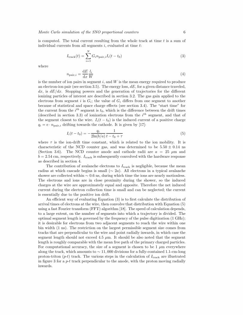
An efficient way of evaluating Equation (3) is to first calculate the distribution ofarrival times of electrons at the wire, then convolve that distribution with Equation (5)using a fast Fourier transform (FFT) algorithm [18]. The speed of calculation depends,to a large extent, on the number of segments into which a trajectory is divided. Theoptimal segment length is governed by the frequency of the pulse digitization (1 GHz);it is desirable for electrons from two adjacent segments to reach the wire within onebin width (1 ns). The restriction on the largest permissible segment size comes fromtracks that are perpendicular to the wire and point radially inwards, in which case thesegment length should not exceed 4.5 µm. It should be also noted that the segmentlength is roughly comparable with the mean free path of the primary charged particles.For computational accuracy, the size of a segment is chosen to be 1 µm everywherealong the track, which amounts to ∼ 11, 000 divisions for a fully-contained 1.1-cm-longproton-triton (p-t) track. The various steps in the calculation of Itrack are illustratedin figure 3 for a p-t track perpendicular to the anode, with the proton moving radiallyinwards.


Figure 3. Calculation of Itrack (3) for a p-t track perpendicular to the anode,with the proton moving radially inwards. The grey distribution shows the energydeposition per unit of length, dE/dx for the proton and triton tracks; the track-distance axis is on the top of the plot, with the origin being the start of protonand triton tracks. The proton travels to the left and the triton to the right. Thepeak in the proton energy deposition is the Bragg peak. The initial triton energyis already below its Bragg peak, so it has a continuously falling distribution. Theblack curve is the distribution of electron arrival times at the wire. This curveappears stretched relative to the energy deposition because of the shape of theelectron drift-time distribution and the difference in drift times for each end ofthe track. The noise on the first two curves is the result of rebinning the tracksegments. The blue short-dashed curve results from applying the gas gains Gi,including space-charge effects; the large noise fluctuations are due to avalanchestatistics. The red long-dashed pulse is Itrack. The effects of the ion drift areadded by convolving (5) with the previous curve; it effectively acts as a low-passfilter, smoothing out the high-frequency fluctuations and adding a long tail to thepulse. All curves are normalized to the same area.

The power of this numerical approach is that any pulse can be computed, giventhe location and number of ionization electrons in the event. Ignoring for the momentvariations in the particle trajectory, it is convenient to formulate pulses as a functionof four variables, in addition to t: Itrack(E, r, θ, φ), where E is the particle energy,r its starting radius, θ the track angle relative to the wire, and φ is an azimuthalangle relative to the radial vector (see figure 4). Figure 5 (top row) shows typicalItrack shapes from the three classes of physics events of interest: a neutron capturingat r = 1.29 cm, with the proton traveling outwards at θ = 67 and φ = 13 (firstcolumn), a 5 MeV alpha particle starting at r = 2.5 cm, with θ = 105 and φ = 14

(second column), and a 5 MeV electron starting at r = 2.5 cm and scattering thriceon the walls before being absorbed in the nickel. A small δ-ray resulting from a Mollerscatter can be seen at (x, y) = (−1.2, 1.5) cm. Track projections onto the radial planeare displayed in the bottom row.

3.2. Ionizing Particles in the NCD Counters


r

Triton

Anode

Alpha

Proton

Wall

Counter

θ

θ

(a)

r

5 cm

Counter

Wall

Anode

Alpha

Proton

Triton

φ

φ

(b)

Figure 4. Graphical definition of the angles θ and φ used to parameterize thealpha and p-t tracks. θ is with respect to the z axis, and r always lies in the x− yplane.

Figure 5. Representative pulses from the three classes of ionization events: (a)a neutron, (b) a 5 MeV alpha, and (c) a β particle. The particle trajectoriesviewed in the radial plane are shown in (d), (e), and (f), respectively. The trackcoordinates are given in the text.

3.2.1. Protons, Tritons and Alphas In the energy range of interest (0.2-8 MeV),the energy loss, dE/dx, for protons, tritons and alphas in the NCD counter gas areaccurately calculated by the software package TRIM [19].‡ The mean stopping ranges

‡ TRIM has been extensively verified against measurements of energy loss in He, C, F, and CF4,with agreement at the few-percent level.


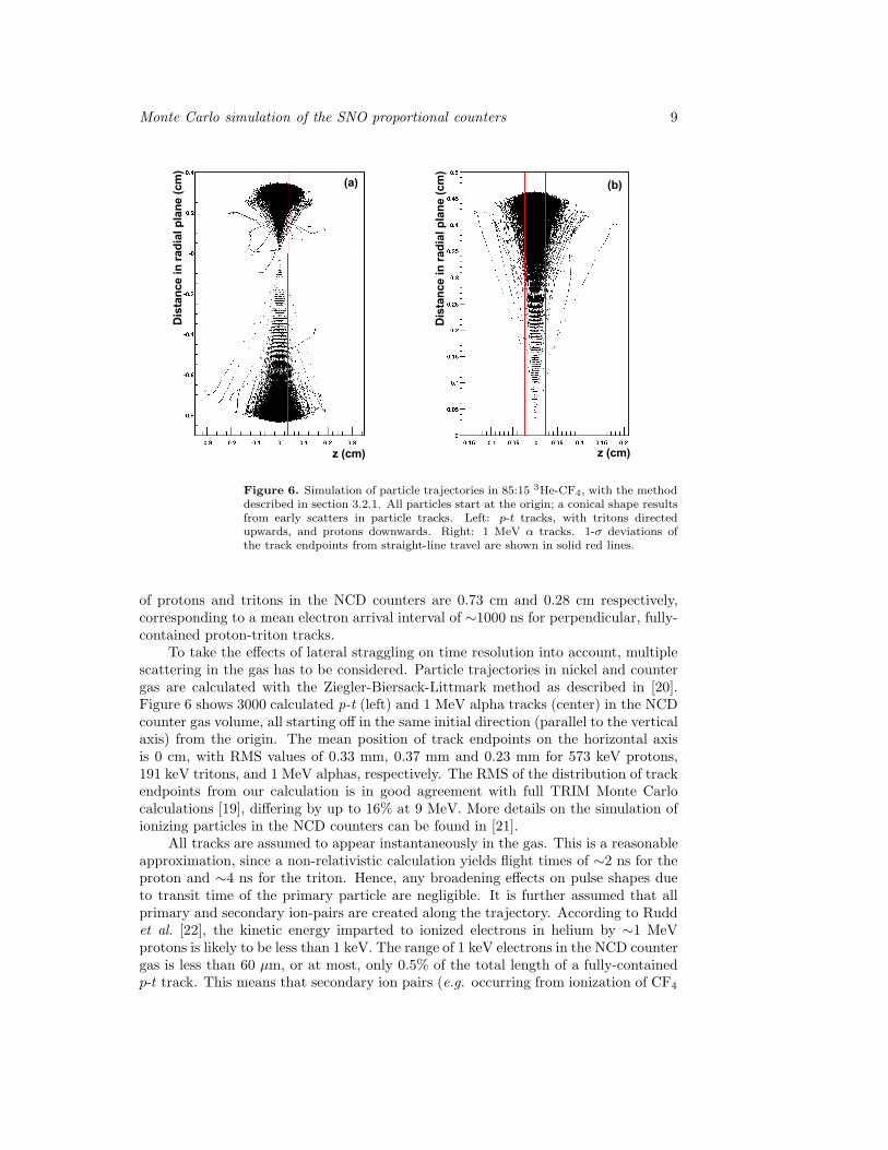
Figure 6. Simulation of particle trajectories in 85:15 3He-CF4, with the methoddescribed in section 3.2.1. All particles start at the origin; a conical shape resultsfrom early scatters in particle tracks. Left: p-t tracks, with tritons directedupwards, and protons downwards. Right: 1 MeV α tracks. 1-σ deviations ofthe track endpoints from straight-line travel are shown in solid red lines.

of protons and tritons in the NCD counters are 0.73 cm and 0.28 cm respectively,corresponding to a mean electron arrival interval of ∼1000 ns for perpendicular, fully-contained proton-triton tracks.

To take the effects of lateral straggling on time resolution into account, multiplescattering in the gas has to be considered. Particle trajectories in nickel and countergas are calculated with the Ziegler-Biersack-Littmark method as described in [20].Figure 6 shows 3000 calculated p-t (left) and 1 MeV alpha tracks (center) in the NCDcounter gas volume, all starting off in the same initial direction (parallel to the verticalaxis) from the origin. The mean position of track endpoints on the horizontal axisis 0 cm, with RMS values of 0.33 mm, 0.37 mm and 0.23 mm for 573 keV protons,191 keV tritons, and 1 MeV alphas, respectively. The RMS of the distribution of trackendpoints from our calculation is in good agreement with full TRIM Monte Carlocalculations [19], differing by up to 16% at 9 MeV. More details on the simulation ofionizing particles in the NCD counters can be found in [21].

All tracks are assumed to appear instantaneously in the gas. This is a reasonableapproximation, since a non-relativistic calculation yields flight times of ∼2 ns for theproton and ∼4 ns for the triton. Hence, any broadening effects on pulse shapes dueto transit time of the primary particle are negligible. It is further assumed that allprimary and secondary ion-pairs are created along the trajectory. According to Ruddet al. [22], the kinetic energy imparted to ionized electrons in helium by ∼1 MeVprotons is likely to be less than 1 keV. The range of 1 keV electrons in the NCD countergas is less than 60 µm, or at most, only 0.5% of the total length of a fully-containedp-t track. This means that secondary ion pairs (e.g. occurring from ionization of CF4


Figure 7. dE/dx (solid lines) and stopping ranges (dashed lines) of protons(red), tritons (blue), alphas (magenta) and electrons (black) in the NCD countergas volume.

by ionization electrons) are created close to the particle path. The effect on pulseshapes, apart from a minor smearing effect, is negligible.

3.2.2. β Particles The propagation of β particles and γs in NCD counter gas ishandled by the software package EGS4 [23]. The interactions of electrons with theNCD counter gas can be classified in three main categories: (1) inelastic collisions,including excitations and ionizations, (2) elastic interactions with electrons (i.e. Mollerscattering), and (3) Bremsstrahlung. The primary mode of energy loss is via inelasticcollisions with gas particles, which can be evaluated with the Bethe-Bloch formula.The resulting energy loss per unit length, dE/dx, and range are shown in figure 7, asa function of energy. A typical β track contains multiple elastic scatters on the nickelwalls. This widens and complicates the structure of Itrack. On account of the very lowstopping power, most β pulses are low-amplitude and do not trigger the proportionalcounter. The probability of a triggered event resulting from an electron possessingmore than 0.2 MeV of kinetic energy is < 0.1%. The estimated number of detected βevents above 0.2 MeV in SNO’s third phase resulting from U and Th impurities was∼1.3.

3.3. Electron Drift Times

A Monte Carlo-based low-energy electron transport simulation was developed toevaluate the mean drift times, td, of electrons in the NCD counter gas mixture asa function of initial radius. This simulation was used instead of other availablesimulations (such as GARFIELD [24]) because the latter were not well suited for


situations where the electric field varies rapidly (e.g. near the anode wire), or whereelastic scattering interactions are dominant over a wide energy range, such that theelectron takes a relatively long time to equilibrate with the gas.

The electron-transport simulation we developed showed good agreement withGARFIELD predictions in benchmarks using a constant electric field. We alsocompared with past measurements by Kopp et al [25]. Figure 8 shows the 1-σ(cyan/light shading) and 2-σ (green/dark shading) allowed regions for td in a 85:153He-CF4 mixture, conservatively assuming experimental uncertainties of ±10% at allelectric field values (no uncertainties are given in [25]).

Further verifications can be made by inspecting specific types of alpha pulses.These include 5.3-MeV 210Po alphas that deposit between 0.9-1.2 MeV in the gas.The maximum radial length of these events is, on average, 0.12 cm, corresponding toan observed pulse FWHM of ∼400 ns. This means that, if one allows for a broadeningof ∼100 ns by the electronic reflection, the time difference between drift times ofelectrons starting at 2.54 cm and 2.42 cm cannot exceed 300 ns. The dashed curve infigure 8 shows this requirement. A slightly more stringent constraint is obtained byexamining the widest alpha particle events, which originate from the anode (dottedline in figure 8). The drift times were increased by a scaling factor of 10±4% to matchthe calculations to observed pulse-width distributions. Taking all of the above intoaccount, the drift time curve for the NCD counter simulation, as a function of radius,is:

td = 121.3r+ 493.9r2 − 36.71r3 + 3.898r4 (6)

with td in ns and r in cm. The uncertainty on td(r) was conservatively assumed to be±10%, based on the agreement of the data and simulations shown in figure 8.

Electron diffusion results in a radius-dependent smearing on all pulses, anddominates the time resolution. A smearing factor σD is determined as a functionof r from the electron-drift simulation, and is applied in pulse calculations. σD and tdare found to be linearly related:

σD(td) = 0.0124td + 0.559 (7)

The differences between the drift curves and the electron diffusion for 3He gas and4He gas were found to be insignificant compared to the uncertainties in the model.

In the endcap regions of the NCD counters the electric field is not purelycylindrical (i.e. radial in the x − y plane and constant along the z axis). Electronswere not propagated in the non-cylindrical-field region, since we do not know howthe drift speeds or gas gain are affected. The line determining approximately wherethe field transitioned from cylindrical to non-cylindrical was determined with a roughcalculation of the fields in the endcap region. Electrons from particles in the non-cylindrical-field region were not propagated. We estimate that approximately 1% ofall neutron and alpha pulses were affected by the endcap region. The impact of thesepulses in the data analysis is discussed in section 5.2.

3.4. The Gas Gain

The mean NCD counter gas-gain (averaging over many events in a counter), G, as afunction of voltage, is well described by the Diethorn formula [26]:

lnG =V

ln(b/a)

ln 2

W

(

lnV

pa ln(b/a)− lnK

)

. (8)


radius (cm)

0 0.5 1 1.5 2 2.5

s)µ ( d

mea

n d

rift

tim

e t

0

0.5

1

1.5

2

2.5

3

3.5

This workGARFIELD

Po constraint210

Wire alpha constraint allowed regionσ1- allowed regionσ2-

radius (cm)

0 0.5 1 1.5 2 2.5

s)µ ( d

mea

n d

rift

tim

e t

0

0.5

1

1.5

2

2.5

3

3.585% He - 15% CF4

Figure 8. Mean electron drift time in the NCD counters as a function of radius.The cyan/light shaded region is the set of possible td(r), conservatively assumingexisting measurements [25] to have an uncertainty of ±10% (none were givenin [25]). The green/dark and cyan/light shaded regions combined represent a±20% (2-σ) uncertainty. Regions above the dotted curve are disfavoured by wireα pulses, which require td(r = 2.54cm) < 3451 ns (denoted by the dashed-dottedlines). The dashed curve is a weaker constraint from low-energy 210Po events,while the magenta solid curve is the actual function adopted in pulse simulations.GARFIELD calculations are the red diamond data points.

The Diethorn parameters are the average electric potential change between ionizationevents, W , and the cylindrical electric field,

E(r = rav) =V

ln(b/a)rav. (9)

E depends on the anode voltage, V , the NCD counter’s anode-wire and inner-wall radii,a and b respectively, and the mean avalanche radius, rav. All of these parameters weremeasured for the NCD counters and are listed in table 1.

However, the G can vary in several ways from the array average. These changescan affect the detected energies and pulse shapes. The gain on a particular string canbe different from the array average if, for example, V is slightly different on that string.Within a string, G can vary by counter because of subtle differences in the gas pressureor inner wall radius, b. The spread in gains between the counters was approximately3%. String and counter variations in the mean gas gain were measured with neutroncalibrations, and those variations were implemented in the NCD simulation.


Besides variations in G, during the formation of a current pulse Gi will differ fromG for each track segment, i. There are random statistical fluctuations in the size of anionization avalanche from a single electron. For a mean gas gain of approximately 220,the avalanche size varies exponentially [25]. These fluctuations are easily simulated byrandomly choosing the gas gain from an exponential distribution with mean G. Thiseffect results in a subtle smoothing of the pulse shape.

More significantly from the point of view of energy spectra and pulse shapes, underthe typical NCD array operating conditions (i.e. for anode voltage V = 1950 V) thecharge multiplication is sufficiently high for ion shielding to become non-negligible.The energy spectra and wide-angle (large θ) pulse shapes are substantially modifiedby this so-called “space-charge” effect.

A two-parameter model that accounts quantitatively for the space-charge effectwas implemented. Consider a cluster of ions of total charge, q, formed in an electroncascade close to the wire, located at a mean radius r. The charge induced by theseions on the anode modifies the local wire charge density.§ The change in gas gain, δG,resulting from a change in wire charge density, δλ(r), is derived from (8):

δG ∝ GlnGln(b/a)

2πǫ0V

(

1 +1

ln(rav/a)

)

δλ(r). (10)

δλ is obtained by dividing the induced charge by a characteristic shower width in thespatial dimension parallel to the anode wire, Ws, which, for simplicity, is assumed tobe a constant for all avalanches:

δλ(r) =q

Ws

ln(b/r)

ln(b/a). (11)

Electrons originating from a given segment, i, of a particle track are affected by thedensity changes brought about by ions formed in previous electron cascades, δλj . Eachof these ion clusters moves slowly towards the cathode while the primary electrons arebeing collected. In the presence of many ion clusters, the total change in the anodecharge density at time t, affecting the evolution of the electrons from the ith tracksegment, is therefore:

δλi =e

Ws

i−1∑

j=1

ln[b/rj(t)]

ln(b/a)Gjnpair,j +

e

Ws

ln(b/r)

ln(b/a)npair,i. (12)

npair,j is the number of ion pairs formed in the jth segment, and j loops over all theprevious ion clusters, which have moved to different radii rj(t) at time t. rj(t) issolved by integrating the relation

drjdt

= µE(rj) −→ rj(t)2 =

2µV t

ln(b/a)+ r2av, (13)

with E(rj) being the value of the electric field at rj , and µ the ion mobility.A charge segment cannot have a significant impact on the gain of another segment

if their avalanches are far apart in the z direction. For simplicity the shower widthis assumed to be a step function; an electron shower centered at a position z0 on thewire is only affected by segments collecting within the limits z0 −Ws < z < z0 +Ws.This approximation is crude, but efficient. For those which do overlap, the commondistance between cascades is calculated and the induced charge density weighted byan overlap factor ξ. As an example, a group of electrons arriving at the anode at

§ In the steady state, the anode wire has a global charge density that depends on the applied voltage.


z1 < z0, with z1 + Ws/2 > z0 − Ws/2 has an overlap factor of (Ws + z1 − z0)/Ws.Equation (12) then becomes:

δλi =e

Ws

i−1∑

j=1

ln[b/rj(t)]

ln(b/a)Gjnpair,jξj +

e

Ws

ln(b/r)

lnb/anpair,i. (14)

It is implicitly assumed that ions produced in avalanches induce an image charge ofuniform density along the wire.

The mean gas gain of the ith track segment is, therefore:

Gi = G− δGi. (15)

δGi is evaluated with (10), using (14) as an input.In this numerical model, the two parameters that need to be optimized are: [1] the

constant of proportionality in (10) (referred to as η in table 1), and [2] the avalanchewidth Ws. These two quantities share a strong inverse correlation. Their valuesare determined by tuning the 210Po peak position relative to the neutron peak, theposition of the bump in the 210Po spectrum caused by the space charge relative tothe 210Po peak, and the shape of the neutron spectrum. The parameters Ws and ηare needed to accurately reproduce both neutrons and 210Po alphas, which impliesthat at least one of the two parameters varies with energy. In this model all of theenergy dependence is given to Ws, while η is fixed. Further information about theelectron-drift and gas-gain simulation can be found in [21].

Other physics parameters, such as G, µi, W and rav, are constrainedindependently. They are listed in table 1. The following two sections describe themeasurements made to determine W (section 3.5) and µ (section 3.6).

Table 1. Space-charge model input values. For Ws, the energy E is in MeV, andthe uncertainties for both the gradient and offset are given.

Parameter Value Uncertainty

η 1.5 0.1Ws (µm) 154E + 782 31, 120

G 219 10µ (10−8 cm2/ns/V) 1.082 0.027W (eV) 34 5rav (µm) 58 10

3.5. The Gas Gain and the Average Energy per Ion Pair

Two parameters are primarily responsible for determining the integrated current, I,measured with a proportional counter in response to a given mean amount of energy,E, deposited in the gas: the average energy deposited per ion pair created, W , andthe gas gain, G. Integrating over many current pulses, the relationship between E,W , and G is [26]

W

G=

neE

I, (16)

where n is the rate of neutron captures and e is the electron charge. W is acharacteristic of the ion and the medium in which it is traveling. In this simulationwe have assumed that W is the same for protons, tritons, and alphas; and that W


is independent of energy. This is valid except at low energies, which will have littleeffect on the NCD pulses [27].

To our knowledge W has not been measured before for the gas mixture used inthe NCD counters, but the values for protons and alphas in a variety of other gasesare all fairly similar to each other [27]. To obtain a precise value of W for the SNOcounters, we have measured G/W both in the ion saturation region (low voltage), andat the operating voltage of the NCD counters.

We conducted this test with an undeployed NCD counter. Three radioactivesources were used simultaneously to provide a large neutron flux: 241AmBe, 252Cf, andPu-13C. They were set within approximately 30 cm of the NCD counter with blocksof polypropylene in between to act as a neutron moderator. A layer of aluminumfoil was wrapped around the counter as a Faraday cage to avoid currents inducedon the NCD counter by external electromagnetic fields. The foil was separated fromthe NCD counter body by a layer of plastic bubble wrap, and it was electricallyconnected to ground. The counter was first set up with standard SNO data acquisitionhardware to determine the event rate which, after being corrected for deadtimes, was(429.9± 1.1)Hz.

The second setup replaced the SNO data acquisition system with a picoammeterto read the DC current from the NCD counter. Instead of reading the current fromthe digital display on the picoammeter, which fluctuated rapidly due to statisticalvariations at the low current levels we were measuring, the analog output was fed intoa digital oscilloscope that averaged the reading over periods of a few seconds. It wasfound that the average value would stabilize reliably within that amount of time. Thehigh-voltage supply was connected to the anode wire, and its setting was controlledby the data acquisition system. The picoammeter read the current from the cathode(i.e. the nickel wall of the NCD counter).

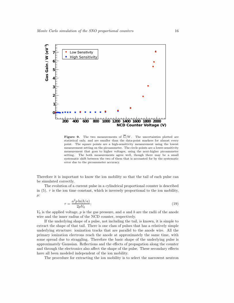
The results from these measurements are shown in figure 9. The lowestmeasurement setting on the picoammeter (range: 2 nA) was able to make a high-sensitivity measurement of the current up to 1500 V, which is shown with the squaresin figure 9. The next-higher current range (20 na) was used to make a lower-sensitivitymeasurement up to 2000 V (circles in figure 9). Due to differences in how the high-voltage supply was calibrated relative to the supplies used in the actual NCD arraysystem, the setting which corresponded to the voltage used for the NCD array was1943.9 V. The data point at this voltage determines G/W to be:

G/W = 6.36± 0.33(stat)± 0.03(syst)eV−1. (17)

Using the value of G = 219 as shown in table 1, W was found to be 34± 5 eV.The high-sensitivity measurements can be used as a comparison. A fit with

a zeroth order polynomial in the ion saturation region, between 200 and 800 V,determines G/W :

G/W = [2.93± 0.65(stat)± 0.84(syst)]× 10−2eV−1. (18)

Since G = 1 in the ion saturation region, we find W = 34.13± 12.4 eV. These resultsare in excellent agreement with each other, and the value of W = 34 ± 5 eV wasimplemented in the NCD array MC.

3.6. Ion Mobility

The small ion mobility, relative to that of the electrons, results in the long tail thatis characteristic of pulses from ionization in the NCD counters, as shown in figure 3.


Figure 9. The two measurements of G/W . The uncertainties plotted arestatistical only, and are smaller than the data-point markers for almost everypoint. The square points are a high-sensitivity measurement using the lowestmeasurement setting on the picoammeter. The circle points are a lower-sensitivitymeasurement that goes to higher voltages, using the next-higher picoammetersetting. The both measurements agree well, though there may be a smallsystematic shift between the two of them that is accounted for by the systematicerror due to the picoammeter accuracy.

Therefore it is important to know the ion mobility so that the tail of each pulse canbe simulated correctly.

The evolution of a current pulse in a cylindrical proportional counter is describedin (5). τ is the ion time constant, which is inversely proportional to the ion mobility,µ:

τ =a2p ln(b/a)

2µV0

; (19)

V0 is the applied voltage, p is the gas pressure, and a and b are the radii of the anodewire and the inner radius of the NCD counter, respectively.

If the underlying shape of a pulse, not including the tail, is known, it is simple toextract the shape of that tail. There is one class of pulses that has a relatively simpleunderlying structure: ionization tracks that are parallel to the anode wire. All theprimary ionization electrons reach the anode at approximately the same time, withsome spread due to straggling. Therefore the basic shape of the underlying pulse isapproximately Gaussian. Reflections and the effects of propagation along the counterand through the electronics also affect the shape of the pulse. These secondary effectshave all been modeled independent of the ion mobility.

The procedure for extracting the ion mobility is to select the narrowest neutron


pulses from a calibration data set and fit each pulse with a Gaussian convolved witha reflection and the electronics model. The free parameters in each fit are τ , the threeGaussian parameters (amplitude, mean and width), and the reflection time. A fitexample is shown in figure 10. The generic pulse model fits the peaks well enough toallow for a characterization of the ion tail.

Time (ns)

Pu

lse

Am

plitu

de

(a

rb. u

nit

s)

Figure 10. An example of a fit to extract the value of the ion-tail time constant.

A subset of the AmBe neutron calibration runs were analyzed in this study. Aninitial selection of pulses was made by restricting the ADC charge to be between 100and 150. The neutron peak (764 keV) typically falls between 120 and 130 ADC counts,so these are pulses where neither the proton nor the triton hit the wall. A secondselection cut was based on the width and height of each pulse. The sharpness of apulse can be approximately characterized by the ratio of the amplitude to the width.A cut of 0.5 × 10−4 < amplitude/width (V/ns) < 1 × 10−4 removed 99.36% of thepulses.

Figure 11 shows the results from all of the fits in the data set. The histogram hasa broad peak of successful fits, and a smaller peak at low τ of non-physics backgroundpulses (e.g. spikes from electrical discharges do not have an ion tail). Of the 393pulses fit, 337 (≈86%) are above τ = 2 ns. The main peak was fit to a Gaussianusing a log-likelihood minimization because of the small number of entries in many ofthe bins. The mean of the Gaussian fit is τ = 5.50 ± 0.14 ns (σ = 2.15 ± 0.12 ns).The uncertainty is the statistical uncertainty of the fit for τ (the effects of changingthe pulse-selection criteria were small compared to this uncertainty). This resultis expected to be correlated with the time constants of the electronics, which weremeasured ex situ (i.e. the RC constants discussed in section 4).

The time constant corresponds to a mean ion mobility of µ = (1.082± 0.027)×10−8 cm2 ns−1 V−1. This value of the ion mobility was implemented in the NCD


(ns)τ0 2 4 6 8 10 12 14

Co

un

ter

per

0.1

5 n

s

0

2

4

6

8

10

12

14

16

18

20

22

Figure 11. Fit results for the ion-tail time constant. The data set includes393 pulses. The low-τ peak is due to non-physics background pulses. By fittinga Gaussian to the main peak with a log-likelihood minimization the ion timeconstant is determined to be 5.50 ± 0.14 ns.

array MC, and the uncertainty was used to calculate its systematic effects.

4. Electronics and Data Acquisition Simulation

4.1. Pulse Propagation in the Counters

In the NCD array simulation, after a current pulse forms on an anode wire, itpropagates along the counter through the NCD cable to the preamplifier. Theamplified pulse is then transferred to the multiplexer system, at which point it issplit between the two data-acquisition paths. One path integrates the pulse with aShaper-ADC to determine the energy deposited in the counter. Its trigger is based onthe pulse integral. The second path is triggered by the pulse amplitude. The pulse islogarithmically amplified and digitized with a sampling rate of 1 GHz. Each recordedpulse is 15 µs long. The electronic and data acquisition components are describedin more detail in [11]. Each current pulse is simulated using a 17,000-element arraywith 1-ns bin widths; a 15,000-element subset of the array is eventually stored inthe standard SNO data structure for each pulse that causes a trigger. The extra2,000 array elements are used to ensure that the beginning and end of each pulseare treated as if the current from the NCD counter exists continuously beyond the15-µs-long pulse. The start of the recorded 15-µs pulse is determined by the triggerconditions, downstream of the pulse simulation. Figure 12 shows a simulated neutronpulse at various stages of the electronics simulation.


Time (ns)2000 2500 3000 3500 4000

Cu

rren

t (A

rb. U

nit

s)

0

2

4

6

8

10

12

14

16 No Electronics

Before Preamplifier

After Preamplifier

Before Logarithmic Amplifier

Final

Figure 12. A simulated neutron pulse (r = 1 cm, θ = 90, φ = 0) at differentstages of the electronics simulation to show the effects of the different components.The most significant changes to the pulse shape are due to propagation in the NCDcounters, and the logarithmic amplification (∆t in (23)). The shift of the start ofthe pulse is the time delay in the logarithmic amplifier. The preamplifier, on theother hand, has little effect on the pulse shape.

4.2. Electronics simulation

Propagation of the pulse along the NCD string is simulated with a Lossy TransmissionLine (LTL) model [28]. Figure 13 is a diagram of the LTL-model circuit. Half of thepulse is propagated down the NCD string, through the delay line, and back to thepoint of origin of the pulse. The delay line attenuation is also simulated as a LTL.Both halves of the pulse (reflected and direct) are subsequently transmitted up to thetop of the NCD string. The attenuation of the pulse due to transmission along theNCD string is dependent on the distance traveled, so pulses starting at different zpositions will look slightly different when they exit the string.

L R

GC

Figure 13. Circuit diagram for the Lossy Transmission Line model, showing theinductance (L), resistance (R), capacitance (C), and conductance (G).

The simulation parameters for the NCD counter wire and delay line come fromfitting the LTL model implemented with the SPICE simulation package [29] to ex situ

electronics calibration data. The best fit parameters are given in table 2. Skin effects inthe anode wire, the resistances for the counters, and the delay lines result in frequency-dependent values for the parameters of the LTL model. To take the frequency


dependence into account, the measured resistance (R, in Ω/cm) is fit between 0 and200 MHz with an empirical formula that illustrates the DC and frequency-dependentcontributions:

R(f) =A

exp[(f −B)/C] + 1+

D√f + E

exp[(B − f)/C] + 1, (20)

where the fit parameters, A, B, C, D, and E are given in table 2, and the frequencyis given in MHz.

A LTL model using parameters calculated analytically, assuming an infinitecylindrical geometry, gave somewhat different results. However, since the analyticalmodel did not include the effects of counter endcaps, junctions, and the frequency-dependent permeability of the nickel walls, the SPICE fit was deemed superior, andthose parameters were chosen for usage in the NCD array simulation.

Table 2. The parameters used in the Lossy Transmission Line model of theNCD counters and of the delay line. The resistance parameters are not allresistances because, as is shown in (20), parameters B and C determine thefrequency dependence of the different contributions.

Parameter Value

Counter

Inductance (10−8 H/cm) 1.33Capacitance (10−14 F/cm) 7.68Conductance (S/cm/MHz) 0.0

Delay Line

Inductance (10−7 H/cm) 9.91Capacitance (10−12 F/cm) 5.53Conductance (10−12 S/cm/MHz) 3.0

Counter and Delay Line

Resistance - A (Ω/cm) 0.1024Resistance - B (MHz) 13.4Resistance - C (MHz) 8.4

Resistance - D (10−2 Ω/cm/√MHz) 1.643

Resistance - E (10−2 Ω/cm ) 2.32

Propagation in the NCD cable is simulated with a low-pass filter with anRC ≈ 3 ns. There is a small reflection of 15% magnitude at the preamplifier inputdue to the slight impedance mismatch between the preamplifier input and the cable‖.The fraction of the pulse that reflects off the preamplifier input travels to the bottomof the cable, reflects off the top of the NCD string, and subsequently travels back upthe cable.

The preamplifier converts the current pulse to a voltage pulse, with a gainof 27500 V/A. The circuit elements of the preamp also affect the shape of thepulse. We simulate this with a low-pass filter (RC ≈ 22 ns) and a high-pass filter(RC = 58,000 ns). The RC constants were measured by fitting the model to ex-situ

injected pulses.

‖ The frequency-dependence of the reflection coefficient is not known, and it was assumed to beconstant. The 15% reflection coefficient was found to match the data well


The implementation of the low- and high-pass filters performs the calculation in asingle loop over the pulse array (∝ N , N = 17, 000 elements). Furthermore, in the casewhere the RC constant approaches the size of the bin width, the bins are subdividedto maintain the accuracy of the simulation. The low-pass filter is implemented asfollows:

V 0 =d

2τRC

V0

V i =

(

V i−1 +d

2τRC

Vi−1

)

ed/τRC +d

2τRC

Vi, i ∈ [1, N) (21)

where V and V are the pulse before and after passing through the filter, respectively. dis the bin width and τRC is the RC time constant. The high-pass filter implementationis similar:

V 0 =

(

1− d

2τRC

)

V0

V i =

[

V i−1 −(

1 +d

2τRC

)

Vi−1

]

ed/τRC +

(

1− d

2τRC

)

Vi (22)

The multiplexer branch of the electronics chain consists primarily of a ∼ 300-nsdelay cable, a logarithmic amplifier, and a digital oscilloscope. The frequency responseof the delay cable and the electronics between the preamplifier and the logarithmicamplifier are simulated with a low-pass filter (RC ≈ 13.5 ns). The analytic form ofthe logarithmic amplification is

Vlog(t) = a log10

(

1 +Vlin(t−∆t)

b

)

+ cchan + VPreTrig, (23)

where Vlog and Vlin are the logarithmic and linear voltages, respectively, and a, b,cchan, ∆t, and VPreTrig are constants determined by regular in situ calibrations duringdata taking. The circuit elements after the logarithmic amplification are simulatedwith the final low-pass filter (RC ≈ 16.7 ns). The RC constants for the two low-passfilters in the multiplexer simulation were determined by fitting the model to pulsesinjected into the components ex situ. The final element of the multiplexer branch ofthe simulation is the digital oscilloscope. The pulse array values are rounded off tothe nearest integer to replicate the digitization.

4.3. Noise simulation

There are a variety of electronic noise sources within the NCD system. Due to thedifficulty of identifying and measuring all of the individual contributions, noise isadded to the pulses after the rest of the simulation is complete. This situation alsorequires that noise is added to the multiplexer and shaper branches of the electronicsindependently. For the multiplexer branch, the frequency spectrum of the noise wasmeasured for each channel using the baseline portions of injected calibration pulses.This provides the mean value, µi, of the noise power spectrum at each frequency.Assuming that the real and imaginary components of the noise are independentGaussian-distributed random variables, then the standard deviation of the noise isrelated to the mean value by

µi = 2σ2i . (24)


To avoid passing the noise through the final low-pass filter in the linear domain, thefinal simulated pulses without noise are “de-logged” (by inverting (23)), convolvedwith the noise, and subsequently “re-logged.”

The Shaper branch of the electronics is simulated by a sliding-window integralof the preamplified pulse. This number is then converted to units of ADC countsby doing an inverse energy calibration. The constants used in the “uncalibration”are the same constants that are used to calibrate the data. Since the shapersimulation acts on electronic-noise-free pulses, noise is added to the shaper valuewith a Gaussian-distributed random number. The mean and standard deviation ofthe noise for each channel were determined by comparing the energy spectra fromin-situ neutron calibrations to the simulated electronic-noise-free energy spectra.The noise characteristics of each NCD string were determined independently. Thetypical RMS noise (in units of ADC values) is 2.0, with a variance of 0.7 (roughlyRMS = 0.012± 0.004 MeV) across the array.

4.4. Trigger simulation

Once all elements of each system are simulated for a given pulse, a trigger decision ismade in the simulation based on whether the MUX or Shaper thresholds are exceeded.The MUX and Shaper systems include independent triggers and the thresholds forboth are determined by in-situ calibrations. After a MUX trigger, the system isopen for further triggers for 15 µs, after which all MUX channels are dead for1 ms. The oscilloscope recording the pulse is dead for 0.9 s after it is recorded (theother oscilloscope is still live, provided it is not already reading out an event). Theoscilloscope used to read out an event is determined by which is not busy, or bytoggling between them if neither is busy. After a shaper trigger, the system is open tofurther triggers for 180 ns, after which all shaper channels are dead for 350 µs. Thesetimes are only simulated within each Monte Carlo event and not between events. Forinstance, a single Monte Carlo event can involve the spontaneous fission of a 252Cfnucleus during a calibration. Such a fission releases multiple neutrons and will resultin multiple multiplexer and shaper events. The dead-time will be then simulated, butit will not apply between multiple 252Cf events.

All NCD-system triggers are then integrated with the SNO photomultiplier(PMT) signals. The PMT trigger simulation time-orders an array of all PMT signals(i.e. each individual hit on a PMT) in a Monte Carlo event and scans through it todetermine if any of the trigger conditions are satisfied (the trigger window is 430 nslong). If that occurs, then a “global trigger” is created and the simulated data isrecorded. The NCD array signals (i.e. each pulse from the NCD system) are integratedwith the PMT trigger simulation by inserting each NCD signal into the time-orderedarray of PMT signals. As the simulation scans over the combined PMT+NCD signals,any individual NCD signal is sufficient to cause a global trigger.

4.5. Shaper-Only Simulation

Certain parts of the full NCD simulation described above are relatively slow due to thenumber of calculations that must be made. For instance, the space-charge simulationrequires a nested loop over the segments of an ionization track, performing calculationsof the effects on the gas gain ∼ N2 times, where N = 17, 000. The electronics anddata acquisition simulation also include several ∝ N and ∝ N

√N loops over the


pulse arrays. For efficiency purposes when full pulses or an accurate energy spectrumare not needed, we have implemented a fast alternative to the full simulation. Theionization track is simulated to determine the timing of the event and the energydeposited in the gas. That energy is converted directly to an approximate Shapermeasurement by smearing it with a Gaussian to roughly account for the missing physicsand electronics response. The principal component of the NCD-phase analysis [12] thattook advantage of the Shaper-only simulation was the determination of the neutron-detection efficiency. On the other hand, the simulation of the alpha energy spectrumfor the solar-neutrino analysis required the full pulse simulation.

5. Impact and Implementation of the NCD Array Simulation

5.1. Tuning

We tuned and validated the NCD array simulation by comparing simulated pulses tocalibration data using a number of pulse-shape variables:

(i) The physics model and detector response were tuned and validated by comparing24Na neutron calibration data with 24Na neutron simulation [15].

(ii) The string-to-string variation of the alpha contamination was tuned on data abovethe neutron-analysis energy window (above 1.0 MeV) and up to 7.0 MeV, wherea pure alpha sample resides.

(iii) The alpha simulation, including systematic uncertainties, was validated in theregion of interest for the NCD analysis by comparing it with calibration datafrom the alpha strings that were filled with 4He.

This procedure was designed to ensure that the simulation accurately reproduces thedata, without training on a data set that contains the NC neutron signal.

Comparing the simulation to neutron calibration data tests nearly all aspectsof the simulation physics model downstream of the primary energy loss by ions inthe NCD counter gas. We compared simulated and real 24Na calibration data usingthe distributions of a number of pulse-shape-analysis variables. These included shapevariables such as the pulse mean, width, skewness, kurtosis, amplitude, and integral;as well as timing variables, including various rise times (10%-to-50% and 10%-to-90%of the pulse amplitude), integral rise times, and full width at half maximum. Thesecomparisons were used to estimate parameter values and uncertainties for electron andion motion in the NCD counter gas, as well as for the space charge model. After tuning,the agreement between data and simulation in these variables is generally good, asshown in figure 14. Using neutron calibration data to test the level of agreement withsimulation is very valuable because it provides high statistics in the most relevantenergy region for the analysis. Although the first analysis of the data from the NCDarray [12] relied on energy and did not use pulse shape or timing variables, suchcomparisons build confidence that the simulation accurately models the developmentof signal pulses as a function of time, and that the physics is correctly modeled.

To compare data and Monte Carlo in regions of parameter space that containsignificant numbers of alphas, it was necessary to construct a “cocktail” of simulatedalpha pulses with the appropriate mixture of NCD cathode-surface polonium and bulkuranium and thorium alpha events. This step was necessary because the pulse shape,timing, and energy distributions of polonium and bulk alpha events are rather different,as shown in figure 15 and the right-hand plot of figure 18 respectively. Furthermore,


Amplitude

0 0.005 0.010.015 0.02 0.025 0.03 0.0350.04 0.045 0.05

Fra

ctio

n o

f E

ven

ts

0

0.02

0.04

0.06

0.08

0.1

0.12

0.14

Mean (ns)

0 200 400 600 800 1000 1200 1400 1600 1800 2000

Fra

ctio

n o

f E

ven

ts

0

0.02

0.04

0.06

0.08

0.1

10%-90% Rise Time (ns)

0 200 400 600 800 1000 1200 1400 1600 1800 2000

Fra

ctio

n o

f E

ven

ts

0

0.05

0.1

0.15

0.2

0.25

Full Width Half Maximum (ns)

0 500 1000 1500 2000 2500 3000

Fra

ctio

n o

f E

ven

ts

0

0.02

0.04

0.06

0.08

0.1

0.12

Figure 14. Comparison of pulse shape variables in 24Na neutron calibrationdata (black points) and the NCD array Monte Carlo (cyan curve) in the neutronenergy window, 0.4 to 1.2 MeV, with statistical errors only. From top left tobottom right: fraction of events as a function of pulse amplitude, time-axis meanof the pulse, 10%-90% rise time, and full width at half maximum. All distributionsare normalized to unit area.

the polonium-to-bulk ratio varies significantly from string to string, as does the totalnumber of alpha events. We estimated the fraction of polonium and bulk alpha eventson each string by fitting each string’s energy distribution in the region of 1.2 to 7.0 MeVwith simulated polonium and bulk alpha-energy probability distribution functions(PDFs). We chose to fit in energy for two reasons: (1) this variable provides excellentdiscrimination between surface polonium and bulk radioactivity, as can be seen in theright-hand plot of figure 18; (2) we found that energy is quite a robust variable againstchanges in Monte Carlo physics models. The latter point is not surprising since theenergy depends on the total charge deposited in the counter. Therefore to first orderit is independent of the details of the charge deposition process, unlike pulse-shapeand timing variables.

Before the energy-spectrum fit, we calibrated the Monte Carlo energy for eachstring such that the peak of the polonium energy distribution in Monte Carlo matchesthat in data. The size of the calibration constant (essentially an extra gain factor,applied as a multiplicative scale to the event energy) is typically 1-3%, and is differentfor each string. After the fit, we calculated an event weight, w(string, αtype), whichis a function of string number and alpha type (polonium, uranium, or thorium)


describing the best-fit fraction of alphas on each string due to each source.¶ Ingeneral, polonium comprised ∼60% of the alpha population, however there were ±20%(absolute) variations between strings. The weights for the best-fit alpha fractions, andthe data/MC energy scale correction, were applied on an event-by-event basis in theanalysis.

We validated the resulting cocktail alpha simulation by comparing with alpha datafrom the four 4He-filled strings, from 0.4 to 1.2 MeV, and from the thirty-six 3He-filledstrings, from 1.2 to 7 MeV. This comparison is shown in figure 15 for several pulse-shape-analysis variables of interest. The agreement between the Monte Carlo andalpha calibration data is generally good, and builds confidence that the simulationphysics model describes the alpha background well in the region of interest for thephase-three analysis.

5.2. Identification of Alpha Backgrounds

The fully-developed NCD array Monte Carlo improved our understanding of the alphabackground events in the data. The most common type of alpha event was due toa decaying nucleus in or on the nickel wall of a counter. There should also be someradioactive contamination from the anode wire, although the characteristics of thesepulses had not been well understood before the NCD Monte Carlo was developed.There should also be alpha decays occurring in the endcap regions of the counters.While an alpha travels in the gas in the endcap region, the electrons created as thealpha ionizes the gas do not reach the anode wire because of the silica feedthrough (see[11] for details of the construction of the NCD counters). Once the alpha reaches theregion where the ionization electrons can drift to the anode wire, the drifting electronsmay be affected by the locally-distorted electric field. The shapes of the endcap alphapulses were not well understood previously due to both of these effects. The NCDarray MC was used to characterize both types of minority alpha pulses.

The simulation of anode-wire-alpha pulses is a straightforward extension ofstandard “wall-alpha” pulses. The origin of the alpha particle was set on or in thecopper of the anode wire; the initial direction may be away from or into the wire(since alpha particles with enough energy can pass through the wire and still producea pulse). We simulated both bulk 238U and 232Th, and surface 210Po contaminationsfor the anode wires.

The simulation of endcap alpha pulses had the additional complication of trackingionization electrons in the region where ionization electrons may not reach the anodewire, or where the electric field distortions may affect the pulse shapes. Based ona rough calculation of the fields in the endcap regions we used a conical surface todescribe the boundary where electrons start to drift to the anode. Furthermore, wefound that the field distortions were relatively small and could be ignored for thepurpose of generally characterizing alpha pulses originating in the endcap regions.

Figure 16 shows the pulse-width vs. energy distribution for a variety of simulatedalpha-pulse types and neutrons. Besides the wall-alpha pulses there are also wire-alphapulses and endcap alpha pulses. An isolated population of wire-alpha events extends

¶ The bulk alpha events were assumed to be composed of equal parts uranium and thorium becausetheir energy spectra are very similar. We were unable to measure the ratio of uranium and thoriumon each string with sufficient accuracy because the normalizations of the independent uranium andthorium spectra were highly correlated in every energy fit. A single combined bulk spectrum wasused instead.


Amplitude

0.005 0.01 0.015 0.02 0.025 0.03 0.035

Fra

ctio

n o

f E

ven

ts

0

0.05

0.1

0.15

0.2

0.25 (a)

Mean (ns)

200 300 400 500 600 700 800 900 1000

Fra

ctio

n o

f E

ven

ts

0

0.1

0.2

0.3

0.4

0.5

0.6(b)

10%-90% Rise Time (ns)

0 100 200 300 400 500 600 700 800

Fra

ctio

n o

f E

ven

ts

0

0.1

0.2

0.3

0.4

0.5 (c)

Full Width Half Max. (ns)

0 200 400 600 800 1000 1200 1400

Fra

ctio

n o

f E

ven

ts

0

0.1

0.2

0.3

0.4

0.5

0.6

0.7

(d)

Figure 15. Comparison of pulse shape variables in 4He alpha calibration data(black points) and the NCD Monte Carlo alpha cocktail (grey curve), poloniumalphas (red dashed line), and bulk alphas (green dotted line) in the NCD analysisenergy window, 0.4 to 1.2 MeV. The data points are shown with statistical errors,alpha cocktail Monte Carlo is shown with statistical (hatched) and systematic(grey filled) errors. From top left to bottom right: fraction of events vs. pulseamplitude, time-axis mean of the pulse, 10%-90% rise time, and full width athalf maximum. The data and cocktail distributions are normalized to unit area,while the polonium- and bulk-alpha distributions are normalized to their fractionalcontribution to the alpha cocktail.

from the top of the 210Po-alpha peak, and some of the low-energy pulses are narrowerthan the wall alphas and neutrons. Many of the endcap alpha pulses overlap with thewall alphas, but some of the low-energy endcap alphas are also narrower than the wallalphas and neutrons. The pulse-width vs. energy distributions for simulated eventsin figure 16 can be compared to the distribution for the NCD array data in figure 17.There are clearly populations of events that match up with the wide wire-alpha pulsesand with the narrow endcap alpha pulses. Prior to the full development of the NCDarray MC these populations in the data were not understood. By simulating a varietyof alpha pulse types we were able to identify these unexplained pulses in the data.

5.3. Use in the Solar-Neutrino Signal Extraction

In the SNO Phase-3 analysis [12] the number of events as a function of energy inthe NCD array data were fit with neutron and alpha PDFs simultaneously with thePMT data. The best-fit number of neutrons is proportional to the detected 8B solar-


Figure 16. Pulse-width vs. energy distributions for simulated neutrons (grey)and alphas. The alpha populations include surface wall 210Po alphas (red), bulkwall 238U alphas (magenta), surface wire 210Po alphas (green), bulk wire 238Ualphas (blue), and bulk endcap 238U alphas (black, distributed with the bluepoints).

Energy (MeV)0 1 2 3 4 5 6 7

pu

lse

wid

th a

t 40

% o

f am

plit

ud

e (n

s)

0

0.5

1

1.5

2

2.5

3

3.5

4

4.5

5310×

Figure 17. Pulse-width vs. energy distributions for the NCD array data. Priorto studies with the NCD array MC the populations of extremely wide and narrowpulses were not well understood. By comparing with the simulated data infigure 16 they can be identified as wire-alpha pulses and possibly endcap alphapulses.


neutrino flux plus the deuteron photodisintigration background. The neutron PDFcomes from 24Na calibration data, while the alpha PDF is calculated with the NCDarray simulation described in this paper. Due to the lack of an adequate in-situ alphacalibration, we needed the simulation to produce a data set with sufficient statisticalaccuracy and the correct bulk-to-surface event ratio. We produced a data set withapproximately 10-times the number of alpha events expected in the data from theSNO’s third phase. The final step was to determine the energy-dependent systematicuncertainties for the alpha energy spectrum.

Table 3. Parameters used in the NCD array simulation and their associateduncertainties, listed in descending order of importance. The alpha cocktailfractions, the mean 238U & 232Th depths, and the instrumental background cutsvary from string to string.

Parameter Value Range

Mean Po Depth (µm) 0.1 ± 0.1Mean U & Th Depth Varies VariesInstrumental Background Cuts Varies VariesAvalanche Width Gradient 154 ± 31Avalanche Width Offset 782 ±120Electron Drift Curve (Scaling, %) 10 ± 4Ion Mobility (10−8 cm2 ns−1 V−1) 1.082 ± 0.027Alpha Cocktail Varies Varies

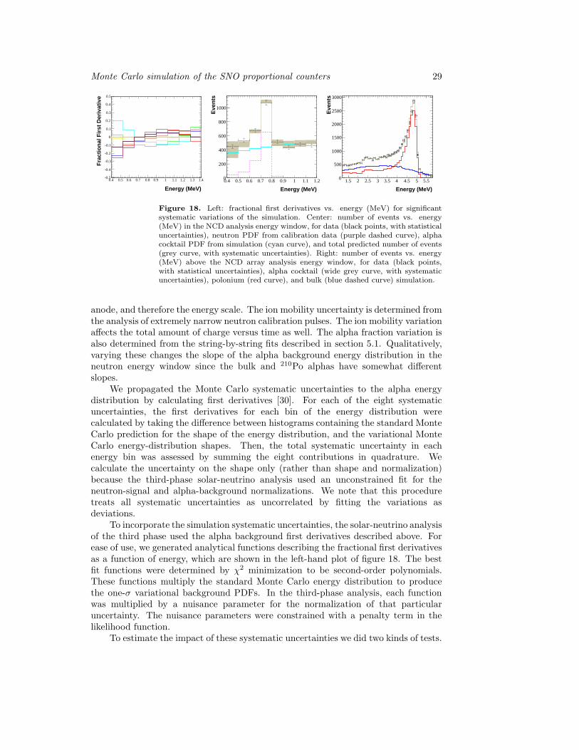
The systematic uncertainties we considered are listed in table 3; these reflectthe range of these parameters in the physics model of the NCD array. Systematicsare assessed by generating large sets of variational Monte Carlo data, each with onesimulation input parameter varied by one σ with respect to its default value, andwith similar statistics to the standard Monte Carlo data set. In the standard MonteCarlo data all parameters are fixed to their default values. No other parameters,including energy scale and polonium/bulk fractions, are different between the defaultand variational Monte Carlo sets. The size of the systematic-parameter variationsfor the NCD array Monte Carlo were estimated from ex-situ, off-line measurementsof the NCD array signal processing electronics response, and in-situ constraints fromthe NCD array data. In the latter case, we used orthogonal data sets to assess thevariations, either from calibration data, or from the data set above 1.2 MeV.

The 1-σ uncertainties for the selected systematic parameters were determinedin different ways. As described in section 5.1, the uncertainty on the alphacocktail fractions comes from the high-energy fits. The alpha-depth uncertaintiesare conservatively assumed to be the difference between the best-fit values for themean depths and completely uniform/surface distributions. Qualitatively, varyingthe alpha depth changes the slope of the energy distribution in the neutron windowbecause the width and the amplitude of the pulses depend on the origin of the alphaparticles. We fit the mean depths using alpha data above the neutron analysiswindow. The uncertainty on the electron drift curve scaling is estimated from theanalysis of the widest wire alphas, since this variation tends to change the averagepulse width. The uncertainties on the space-charge offset and gradient parameters,which are the coefficients of W∫ described in section 3.4, are determined by lookingat how the features of the alpha energy spectrum shift as each parameter is changed.Qualitatively, tuning these parameters changes the charge deposited versus time on the


Energy (MeV)

0.4 0.5 0.6 0.7 0.8 0.9 1 1.1 1.2 1.3 1.4

Fra

ctio

nal

Fir

st D

eriv

ativ

e

-0.5

-0.4

-0.3

-0.2

-0.1

0

0.1

0.2

0.3

0.4

0.5

Energy (MeV)

0.4 0.5 0.6 0.7 0.8 0.9 1 1.1 1.2

Eve

nts

0

200

400

600

800

1000

Energy (MeV)

1.5 2 2.5 3 3.5 4 4.5 5 5.5

Eve

nts

0

500

1000

1500

2000

2500

3000

Figure 18. Left: fractional first derivatives vs. energy (MeV) for significantsystematic variations of the simulation. Center: number of events vs. energy(MeV) in the NCD analysis energy window, for data (black points, with statisticaluncertainties), neutron PDF from calibration data (purple dashed curve), alphacocktail PDF from simulation (cyan curve), and total predicted number of events(grey curve, with systematic uncertainties). Right: number of events vs. energy(MeV) above the NCD array analysis energy window, for data (black points,with statistical uncertainties), alpha cocktail (wide grey curve, with systematicuncertainties), polonium (red curve), and bulk (blue dashed curve) simulation.

anode, and therefore the energy scale. The ion mobility uncertainty is determined fromthe analysis of extremely narrow neutron calibration pulses. The ion mobility variationaffects the total amount of charge versus time as well. The alpha fraction variation isalso determined from the string-by-string fits described in section 5.1. Qualitatively,varying these changes the slope of the alpha background energy distribution in theneutron energy window since the bulk and 210Po alphas have somewhat differentslopes.

We propagated the Monte Carlo systematic uncertainties to the alpha energydistribution by calculating first derivatives [30]. For each of the eight systematicuncertainties, the first derivatives for each bin of the energy distribution werecalculated by taking the difference between histograms containing the standard MonteCarlo prediction for the shape of the energy distribution, and the variational MonteCarlo energy-distribution shapes. Then, the total systematic uncertainty in eachenergy bin was assessed by summing the eight contributions in quadrature. Wecalculate the uncertainty on the shape only (rather than shape and normalization)because the third-phase solar-neutrino analysis used an unconstrained fit for theneutron-signal and alpha-background normalizations. We note that this proceduretreats all systematic uncertainties as uncorrelated by fitting the variations asdeviations.

To incorporate the simulation systematic uncertainties, the solar-neutrino analysisof the third phase used the alpha background first derivatives described above. Forease of use, we generated analytical functions describing the fractional first derivativesas a function of energy, which are shown in the left-hand plot of figure 18. The bestfit functions were determined by χ2 minimization to be second-order polynomials.These functions multiply the standard Monte Carlo energy distribution to producethe one-σ variational background PDFs. In the third-phase analysis, each functionwas multiplied by a nuisance parameter for the normalization of that particularuncertainty. The nuisance parameters were constrained with a penalty term in thelikelihood function.

To estimate the impact of these systematic uncertainties we did two kinds of tests.


First, we estimated the errors on the pulse shape and timing distributions to giveguidance on which variables are most robust against NCD array Monte Carlo physicsmodel uncertainties. We found that some variables were much more sensitive to certainsystematic variations than others. For example, the space-charge model parametersprimarily affect the rise-time distributions, while the alpha-depth variations have alarge effect on most variables. Second, we fit the energy spectrum of an unknownfraction of the data (to maintain blindness) to determine the number of neutronsbetween 0.4 to 1.2 MeV, using each of the variational Monte Carlo sets as the alpha-background PDF. The variation in the number of neutrons provided the most relevantestimate of the uncertainty, and possible bias, due to each systematic source. Ingeneral, these fits showed that the alpha depth variation systematic uncertainty hasthe largest impact, followed by the noise model, the electron drift time curve, and theion mobility variation. The total systematic uncertainty assessed in this way on thenumber of neutrons was approximately 4%.

The final simulated alpha energy spectrum in the analysis energy window is shownin the center plot of figure 18, with systematic uncertainties. This alpha spectrum wasused as the background PDF in the third-phase analysis, together with the neutronsignal PDF from 24Na neutron calibration data, to extract the best-fit total numberof neutron events.

5.4. Pulse Fitting

Another approach to separating neutron and alpha events is to fit individual pulseswith neutron and alpha template pulses. In particular, we can use the NCD arrayMonte Carlo to generate libraries of such templates for both the signal neutrons andalpha backgrounds.+ A library of simulated pulses consists a set of a single class ofpulses (either neutrons, wall alphas, or wire alphas), where the pulse shapes includedcover as many of the available pulse shapes as possible. The parameter space for theavailable pulse shapes consists of five variables: the radius, r, the two track angles, θand φ, the position along the NCD string, z, and the initial energy, E. A data pulseis fit by finding the best match in the library.

The three types of events, neutrons, wall alphas, and wire alphas, are cataloguedin separate libraries. The three libraries are generated by varying the parameterson the four-dimensional grids in their respective parameter spaces. For neutrons therelevant coordinates of the parameter space are r, θ, φ, and z. The initial energyis fixed at 574 keV and 191 keV for the proton and triton, respectively. For alphasthe relevant coordinates are E, θ, φ, and z, with the radius fixed at either the innerradius of the wall or the outer radius of the wire (the pulse shape for any alpha leavingthe wall with a given E, θ, φ, and z will be the same regardless of whether or not itstarted out deeper in the nickel or on the surface). Table 4 shows the grids used in thepulse-shape parameter spaces, and table 5 shows the numbers of pulses in the threelibraries. Further details about the creation of the pulse libraries can be found in [32].

When comparing a data pulse to a library of simulated pulses, the quality of eachfit is determined by a Pearson’s χ2 test. The library pulse that has the smallest χ2

+ It would be inefficient to generate the pulses as a fit is performed because of the time needed togenerate each pulse. Furthermore, most minimizing routines perform best when the fit function (i.e.the simulated pulse shape) changes smoothly as a function of its parameters (r, E, θ, φ, and z). Thisis not the case in the NCD array simulation when a change of any of those coordinates can cause atrack to hit the wall or wire and therefore change the pulse shape discontinuously.


Table 4. The number of grid points along each dimension in the relevantsimulation parameter space for the three libraries produced. The radius pointsare spaced uniformly in r.

r (cm) Ea (MeV) θ () φb () z (cm)

Range [0.1, 2.5] [0.2, 1.2] [0, 90] c [−535, 535]

Neutron 5 N/A 10 10 10Wall Alpha N/A 10+2d 10 5 10Wire Alpha N/A 10 10 5 10

a This energy is the initial energy of the alpha particle.b The number of φ points depends on θ to uniformly cover the spherical space.The maximum number of φ points is given in this table.c The specific φ range used depended on the geometry relevant for each library.d Two extra grid points are added in energy to account for high-energy ions thatreenter the NCD wall, depositing only some of their energy in the gas.

Table 5. The number of pulses generated and used for the neutron, wall-alpha,and wire-alpha libraries. The number of pulses generated is determined by theparameter-space grids given in table 4. Some pulses were removed because theirdeposited energies were either too high or too low. Pulses in the energy range0.2 < E < 1.2 MeV were kept.

Neutron Wall Alpha Wire Alpha

Generated 3350 4200 3500Used 3329 2974 2599

per degree of freedom (dof) when compared to the data pulse is the best fit to thedata.

The fit region for each pulse is determined by finding where the pulse amplitudedrops to a given fraction of the peak amplitude on the rising and falling edges.The tail of each neutron-capture and alpha pulse quickly becomes dominated by thecharacteristic ion-drift time constants, while the rising edge contains information aboutthe particle that produced the pulse. As a result, the left (rising) and right (falling)edges of the pulse are treated differently. The left edge of the fit region is the point atwhich the pulse crosses 10% of its peak value. 10% of the peak amplitude is typicallyabove the baseline noise, even for low pulses, and almost the entire rise of the pulseis included in the fit region. The right edge of the fit region is the point at which thepulse crosses 30% of its peak value. A larger percentage is chosen for the falling edgethan the rising edge to avoid most of the ion-drift tail, which is almost the same forevery pulse and would therefore make the χ2 parameter less effective in separatingpulse shapes.

The variance used in the χ2 calculation is also determined for each pulse. Thereare four sources of variance that can contribute to the difference between a MC librarypulse and a data pulse:

• Electronic noise: Various parts of the electronics contribute to the backgroundnoise on a pulse. The exact frequency spectrum of that noise depends on thebandwidths of downstream electronics components, but it can be approximatedby taking the RMS of the tail of a pulse about the mean value. In particular,bins 11,000 to 14,999 (from approximately 10.2 to 14.2 µs after the start of the


pulse) are used. This contribution to the variance is the largest of the four.

• Digitization: When the pulse is digitized some uncertainty is added to every binbecause each digitized value could represent a range of actual values. The non-voltage-dependent portion of the digitization variance is already accounted forby taking the RMS of the tail of the pulse. The voltage-dependent portion iscalculated separately.

• Library sparseness: Since the MC libraries are created on grids in the pulseparameter spaces before any fitting is performed, they represent a selection of theavailable pulse shapes. Differences between the best-fit MC library pulse and theactual track parameters of the pulse being fit will add to the variance.

• MC imperfections: Since the MC is not perfect, even if an MC pulse is createdwith the exact same track parameters as a real pulse there will still be differencesbetween the two pulses because the MC is not an exact model.

The digitization contribution to the variance depends on the size of a single stepin the digitizer, ∆:

σ2D =

∆2

12. (25)

This factor, known as “Sheppard’s Correction,” [31] is the correction that would needto be applied to determine the true width of a Gaussian peak in a spectrum thathas been binned. In other words, it is the variance of a uniform distribution, sincethe distribution is uniform within a bin. The logarithmic amplification of the NCDarraypulses makes ∆ voltage dependent. It is also dependent on the characteristics ofthe logarithmic amplifiers that go into the analytic description of the amplification,(23). A change of input voltage by ∆ results in a change of Vlog by 1 digitization unit:

Vlog(t) + 1 = a log10

(

1 +Vlin(t−∆t) + ∆

b

)

+ cchan + VPreTrig. (26)

Solving for ∆, and substituting into (25), the contribution to the variance due todigitization is:

σ2D =

1

12

(

Vlin(t−∆t) + b

a log10 e

)2

. (27)

Equation (27) can be expanded and separated into two voltage-dependent terms, anda voltage-independent term. The latter is a part of the variance that is calculatedby taking the RMS of the noise in the tail of each pulse. The voltage-dependentcomponent of the digitization variance turns out to be a relatively small contributionto the total variance. It is an order of magnitude smaller than the voltage-independentvariance (including the electronics and part of the digitization), for pulses with largeamplitudes (and therefore the largest digitization variance).

Unfortunately there is no well-defined method for quantifying the contributionsto the variance from the sparseness of the libraries or the imperfections in the MC. Westudied the increase in the mean reduced χ2 as a result of these two contributions byfitting simulated and real 24Na neutron pulses with the neutron library. The librarywas used to fit a simulated 24Na neutron data set; the excess χ2/dof above 1 wasa result of the variance contribution from the library sparseness. The library wasthen used to fit a real 24Na neutron data set, and the excess χ2/dof above the valuefrom fitting the simulated data was a result of the variance contribution from MC


imperfections. We found that their contributions were small and had no significantimpact on the ability to separate neutron and alpha pulses.

An energy term of the form (E − Efit)2/V [E] is also added to the χ2 statistic to

take into account the difference in energy between the library pulse and the pulse beingfit. The variance for the energy term is set by the alpha-library energy spacing, ∆Eα:V [E] ≡ (∆Eα/2)

2. For the libraries used, ∆Eα = 0.1MeV. This factor has a smalleffect on the total χ2 when the difference between the energies is small, particularlysince the number of bins in each pulse’s fit region is large.

We first fit simulated data with the pulse libraries. Figure 19 shows an exampleMonte Carlo neutron pulse fit with both the neutron library and the alpha library(the latter is a combination of the wall- and wire-alpha libraries), accompanied by therespective fit residuals. Figure 20 shows a fit of an alpha Monte Carlo pulse with theneutron and alpha libraries. The neutron pulse selected is fit well with the neutronlibrary (χ2/dof = 0.58, with approximately 1070 degrees of freedom) and fairly wellwith the alpha library (χ2/dof = 0.97). Qualitatively, it is clear that the fit with theneutron library better represents the overall structure of the pulse. Some neutronshave a more generic pulse shape and are fit reasonably well with both the neutron andalpha libraries. The alpha pulse, as is the case with most alpha pulses, fits well withboth libraries (χ2/dof = 0.267 for both fits).

Figure 19. An example of a Monte Carlo neutron pulse fit with the neutronlibrary (a), and the same pulse fit with the alpha library (b). The vertical bluelines indicate the fit region, in which the χ2 was calculated. The χ2 in (b) islarger than in (a), though this example serves to show how a neutron pulse (evenone that is not extremely narrow) can still be fit fairly well with the alpha library.Plots (c) and (d) are the respective fit residuals.

Fitting calibration neutrons and 4He alpha pulses with the simulated-pulselibraries is a strong test of the data-MC agreement. Figure 21 shows two examples:(a) a 24Na neutron pulse and (b) a 4He alpha pulse fit with the neutron and alphalibraries, respectively ((a) χ2/dof = 0.319; (b) χ2/dof = 1.091). In general, these fits


Figure 20. An example of a Monte Carlo alpha pulse fit with the neutronlibrary (a), and the same pulse fit with the alpha library (b). The vertical bluelines indicate the fit region, in which the χ2 was calculated. Alphas tend to be fitwell with both the neutron and alpha libraries, as is the case with this example.Plots (c) and (d) are the respective fit residuals.

work well.

Figure 21. (a) A pulse from the 24Na data set fit with the neutron library and(b) a pulse from the 4He strings fit with the alpha library. The blue lines indicatethe fit region, in which the χ2 was calculated. Plots (c) and (d) are the respectivefit residuals.


The fit results can be used to separate neutron and alpha events because low-energy alpha pulses (< 1 MeV) resemble neutron pulses, but a significant fraction ofthe neutron pulses look distinctly different than any alpha pulse. The comparison ofthe fit results, χ2

α versus χ2n, where χ2

α is the result of the fit with the alpha library,and χ2

n is the result of the fit with the neutron library, is an effective discriminatorof different pulse classes. Figure 22 shows the distributions of logχ2

α versus logχ2n for

calibration neutrons, 4He-string alphas, and the NCD-phase data set. The alphas aregrouped along the χ2

α = χ2n line, as are some of the neutrons. There is a large group

of neutron pulses that fit better with the neutron library than with the alpha library.The one-dimensional projection ∆ log(χ2) ≡ log(χ2

α)− log(χ2n) is more useful for

seeing the ability to select a sample of neutrons with almost no alpha background.This projection is shown in figure 23. The peak on the left is due to alpha and alpha-like neutron pulses. The wider distribution of neutrons on the right is the sample ofneutron pulses that are easily distinguished from alpha pulses. These neutron pulsescan be selected and analyzed with little background alpha contamination. This typeof pulse-shape analysis has the potential to increase the signal-to-noise ratio in theextraction of the number of neutrons detected in future analyses of SNO phase-threedata. The details of such an analysis are beyond the scope of this paper, but can befound in [32]. The simulation-based pulse-shape analysis is being considered for usein the final SNO three-phase analysis [33].

Figure 22. Comparison of the fit results for fitting neutrons and alphas withthe simulated neutron and alpha pulse libraries. The axes are logχ2

αversus

logχ2n. The neutrons are from 24Na calibrations, and the alphas are from the

4He strings. The full NCD-phase data set is also plotted. The 24Na calibrationdata are comprised of approximately 36-times the expected number of neutronsin the phase-three data, and the 4He alpha data are comprised of approximatelyhalf as many alphas expected in the NCD-phase data. There is a subset of theneutron pulses which can be selected with little contamination from alpha pulses.


/dof)2! log("

-0.4 -0.2 0 0.2 0.4 0.6 0.8 1 1.2 1.4

No

rmali

zed

Co

un

ts

-510

-410

-310

-210

-11024Na 2006

NCD Data

4He Alphas

Figure 23. The fit results from the previous figure projected along the∆ log(χ2) ≡ log(χ2

α) − log(χ2

n) axis. The wide distribution of neutron pulses

on the right can be selected with little alpha background. The histograms arenormalized to unit area.


6. Conclusions

We have developed a unique and detailed simulation of the current pulses from theNCD proportional counters. The simulation model includes energy loss by particlestraveling through the NCD counter gas, walls, endcaps, and wire, as well as energystraggling. In the gas, the simulation includes ion drift and electron diffusion. Nearthe anode wire, the simulation models avalanche multiplication and the effects of spacecharge. The signal processing chain model includes the full NCD array data-acquisitionelectronics response, and its associated frequency-dependent noise.

The simulation accurately models the current pulse shapes collectively andon a pulse-by-pulse basis, for both signal neutrons and background alphas. Firstprinciples calculations are used for the majority of the simulation physics. Somemodel parameters are measured with calibration data, and others are parameterizedto match neutron calibration and high-energy alpha data. The dominant systematicuncertainties on the simulation physics come from the alpha implantation depth inthe NCD counter walls, the electronics noise model, the electron drift time curve, andthe ion mobility variation.

The NCD arrayMonte Carlo simulation has been used to great effect in identifyingclasses of alpha backgrounds, in modeling the energy spectrum for the total alphabackground in the third-phase 8B solar-neutrino measurement [12], and in pulse fittingto help identify neutron and alpha pulses.


References

[1] SNO Collaboration 2000 Nucl. Instrum. Methods A 449 172[2] SNO Collaboration 2009 Phys. Rev. D 80 012001[3] Chen H 1985 Phys. Rev. Lett. 55 1534[4] SNO Collaboration 2001 Phys. Rev. Lett. 87 071301[5] SNO Collaboration 2002 Phys. Rev. Lett. 89 011301[6] SNO Collaboration 2002 Phys. Rev. Lett. 89 011302[7] SNO Collaboration 2007 Phys. Rev. C 75 045502[8] SNO Collaboration 2004 PPhys. Rev. Lett. 92 181301[9] SNO Collaboration 2005 Phys. Rev. C 72 055502

[10] SNO Collaboration 2010 Phys. Rev. C 81 055504[11] Amsbaugh J F et al 2007 Nucl. Instrum. Methods A 579 1054[12] SNO Collaboration 2008 Phys. Rev. Lett. 101 111301[13] Mills W R, Jr., Caldwell R L and Morgan I L 1962 Rev. Sci. Instrum. 33 866[14] Firestone R B 1996 Table of Isotopes vol 1 ed Shirley V S et al (New York: John Wiley & Sons,

Inc.) p 1[15] Boudjemline K et al 2010 Nucl. Instrum. Methods A 620 171[16] Cox G A et al 2004 IEEE Trans. Nucl. Sci. 51 2227[17] Wilkinson D H 1950 Ionization Chambers and Counters, (Cambridge, UK: Cambridge University

Press)[18] The FFTW software package, http://www.fftw.org[19] Ziegler J F 2006 TRansport of Ions in Matter, software package[20] Ziegler J F, Biersack J P, and Littmark U 1985 The Stopping and Range of Ions in Solids

(Oxford, UK: Pergamon Press)[21] Wan Chan Tseung H S 2008 Simulation of the Sudbury Neutrino Observatory Neutral Current

Detectors Ph.D. Dissertation (University of Oxford, Oxford, UK)[22] Rudd M E et al 1992 Rev. Mod. Phys 64 441[23] Nelson W R, Hirayama H, and Rogers D W O 1985 The EGS4 Code System, Report SLAC-265,

Stanford Linear Accelerator Center, Stanford, CA[24] Veenhof R Garfield - simulation of gaseous detectors, http://garfield.web.cern.ch/garfield,

software package[25] Kopp M K et al 1982 Nucl. Instrum. Methods A 201 395[26] Knoll G F 2000 Radiation Detection and Measurement, 3rd ed (Hoboken, NJ: John Wiley &

Sons)[27] Int. Comm. on Rad. Units and Meas. 1979 Average energy required to produce an ion pair, ICRU

Report 31[28] King R W P 1955 Transmission-line Theory (New York: McGraw-Hill Book Company, Inc.)[29] SPICE Electronics Design Software, http://www.spice-software.com/index.htm, software

package.[30] Whalley M R and Lyons L 2002 Proc. Conf. on Advanced Statistical Techniques in Part. Phys.

(Durham, UK)[31] Sheppard W F 1898 Proc. London Math. Soc. 29 353[32] Oblath N S 2009 A Measurement of Neutral-Current Neutrino Interactions at the Sudbury

Neutrino Observatory with an Array of 3He Proportional Counters Ph.D. Dissertation(University of Washington, Seattle, WA)

[33] Martin R, Oblath, N S and Tolich N 2010 Pulse-Shape Analysis for the Third Phase of the

Sudbury Neutrino Observatory XXIV International Conference on Neutrino Physics andAstrophysics, Athens, Greece

http://www.fftw.org

http://garfield.web.cern.ch/garfield

http://www.spice-software.com/index.htm

A MonteCarlo simulation of theSudburyNeutrino Observatory ...

Documents