A Monte Carlo Study of Pearson and Log-Linear Chi-Square ...

Loyola University Chicago Loyola University Chicago

Loyola eCommons Loyola eCommons

Dissertations Theses and Dissertations

1979

A Monte Carlo Study of Pearson and Log-Linear Chi-Square One A Monte Carlo Study of Pearson and Log-Linear Chi-Square One

Sample Tests with Small N Sample Tests with Small N

Adam James Miller Loyola University Chicago

Follow this and additional works at: https://ecommons.luc.edu/luc_diss

Part of the Education Commons

Recommended Citation Recommended Citation Miller, Adam James, "A Monte Carlo Study of Pearson and Log-Linear Chi-Square One Sample Tests with Small N" (1979). Dissertations. 1786. https://ecommons.luc.edu/luc_diss/1786

This Dissertation is brought to you for free and open access by the Theses and Dissertations at Loyola eCommons. It has been accepted for inclusion in Dissertations by an authorized administrator of Loyola eCommons. For more information, please contact [email protected].

This work is licensed under a Creative Commons Attribution-Noncommercial-No Derivative Works 3.0 License. Copyright © 1979 Adam James Miller

A MONTE CARLO STUDY OF PEARSON AND LOG-LINEAR

CHI-SQUARE ONE SAMPLE TESTS WITH SMALL N

by

Adam J. Miller II

A Dissertation Submitted to the Faculty of the Graduate School

of Loyola University of Chicago in Partial Fulfillment

of the Requirements for the Degree of <

D6ctor of Education

May

1979

ACKNm·JLEDGrflENTS

The author acknowledges with gratitude the moti­

vation, supervision, and constructive criticism provided

by the Director of the dissertation, Dr. Jack A. Kavanagh.

Dr. Samuel T. Mayo provided the historical, analytical,

and empirical critiques for the philosophical, educa­

tional, and psychological applications of the study. Dr.

Steven I. Miller is thanked for his concern with the socio­

behavioral, educational, and other practical applications

of the research.

The contributions of Miss Sheryl Tutaj, Chicago

Public Relations Officer of IBl":T, and the staff of the York­

town Heights, New York, Research Center are gratefully ac­

knowledged for their participation in program~ing the

generation of random variables from parent chi-square dis­

tributions.

Especial thanks are due Dr. Melvin Cohen and McGill

University for supplying the source deck and instructions

on "How to Use the McGill Random Number Package 'Super­

Duper'" that made this study possible within the time and

money constraints that prevailed.

ii

VITA

The author, Adam James Miller II, is the son of

Adam James l'v1iller, Sr. and Mabel (Hansen) IViiller. He

was born June 23, 1920, in Chicago, Illinois.

His elementary education was obtained in the pub­

lic schools of Chicago, Illinois. His secondary education

was obtained at St. John's r1iili tary Academy, Delafield,

Wisconsin, where he graduated in 1937.

In September, 1937, he entered M. I. T., and in

June, 1941, he received the degree of Bachelor of Science

with a major in Business and Engineering Administration.

While attending M. I. T., he also was a special student

at the Harvard Graduate School of Education during 1939.

From April, 1941, to February, 1944, he was Assis­

tant Plant Engineer and Assistant to the Superintendent

of Hull and Machinery Outfitting at North Carolina Ship­

building Company, a subsidiary of Newport News Shipbuild­

ing and Drydock Company. From February, 1944, to ft'iay,

1946, he served as an Engineering Officer in the United

States Navy Reserve. During this period, as a civilian,

he supervised the construction of the least expensive

Liberty Ship ever built. He also received a commendation

for delivering the least expensive pair of LSM ships at

any navy yard and converted this same type of ship to

iii

missile launchers in minimum time. The last year of

his naval service was spent as Personnel and Engineer­

ing Officer for a division of 990 people, having a

budget of $900,000,000.per annum.

In 1941, he purchased a partnership in a Tex­

aco distributorship, devoting part-time to that enter­

prise as well as devoting himself to other interests,

including employment as a Production Engineer at Chi­

cago Screw Company (1946 to 1948). After that, he

devoted full-time effort to the gasoline distributor­

ship, becoming senior partner and, therefore, president

of the succeeding corporation. From a nadir in 1948,

sales were increased to over $2,000,000 in 1954.

Desiring to return to academia and a teaching

career, the author enrolled as a student in Loyola Uni­

versity of Chicago's Graduate School of Business in

April, 1970. He received the M.B.A. degree with a

major in Quantitative Methods in June, 1971. From June,

1971, to date, he has been a student in Loyola Univer­

sity's Graduate School of Education. In addition, he

served as a Lecturer, Educational Foundations, Loyola

University, in the fall and spring semesters of 1977-

1978.

iv

Table

1.

2.

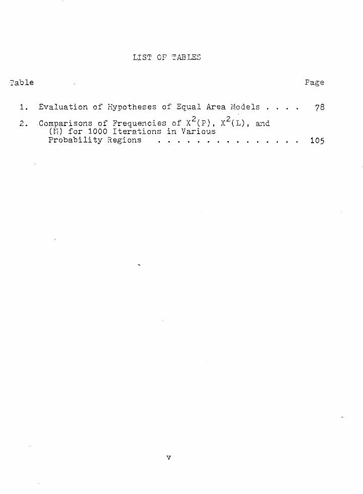
LIST OF TABLES

Evaluation of Hypotheses of Equal Area Models .

Comparisons of Frequencies of X2(P), x2(L), and (N) for 1000 Iterations in Various Probability Regions ......... .

v

Page

78

105

APPENDIX A

APPENDIX B

APPENDIX C

APPENDIX D

APPENDIX E

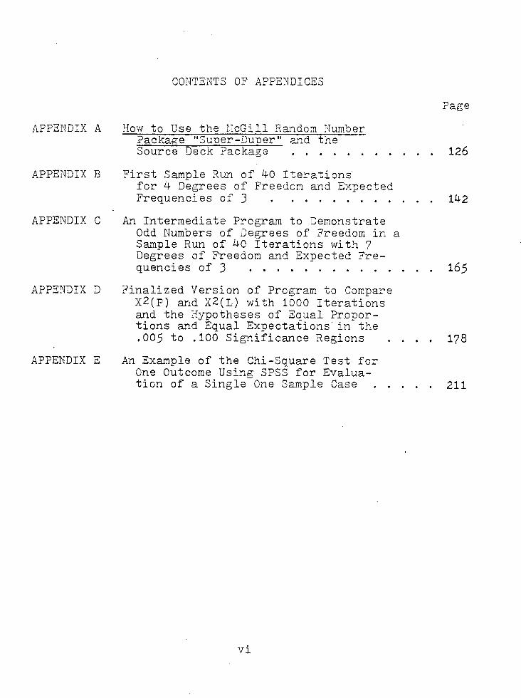
CONTENTS OF APPENDICES

Page

How to Use the f',IcGill Ra'1.dom ~'Tumber Package "Super-Duner" a'1.d the Source Deck Package . . . . . . . . . . . 126

First Sample R.un of 40 Iterations for 4 Degrees of Freedom and Expected Frequencies of J . . . . . . . .

An Intermediate Program to Demonstrate Odd Numbers of Degrees of Freedom in a Sample Run of 40 Iterations with 7 Degrees of Freedom and Expected Fre­quencies of J . . . . . . . . . . .

Finalized Version of Program to Compare X2(p) and X2(L) with 1000 Iterations and the Hypotheses of Equal Pr_opor­tions and Equal Expectations· in the .005 to .100 Significa'1.ce Regions

An Example of the Chi-Square Test for One Outcome Using SPSS for Evalua-tion of a Single One Sample Case . . . . .

vi

142

165

178

211

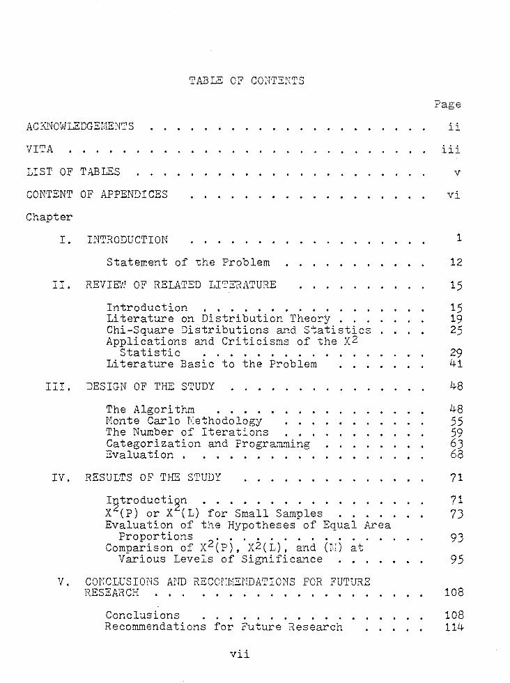
TABLE OF COl,fTE~TTS

Page

A C KN 01iJLEDG ErmNT S . . . . . . . . . . . . . ii

VITA iii

LIST OF TABLES v

CONTENT OF APPENDICES . . . . . . . . . . . . . . . . vi

Chapter

I. INTRODUCTION . . . . . . . . . . . . . . 1

Statement of the Problem . . . . . . . . . 12

II. REVIE'H OF RELATED LITERATURE 15

Introduction . . . . . . . . . . . . . 15 Literature on Distribution Theory . 19 Chi-Square Distributions and Statistics 25 Applications and Criticisms of the x2

Statistic . . . . . . . . . . . . . . . 29 Literature Basic to the Problem . . . 41

III. DESIGN OF THE STUDY

The Algorithm . . . . . . .. l'1ionte Carlo Uiethodology . . . The Number of Iterations . . Categorization and Progranming Evaluation • . . . • . .

IV. RESULTS OF THE STUDY

Introducti~n • . • . . . . . . • . . . . . X2(P) or X (L) for Small Samples ...... . Evaluation of the Hypotheses of Equal Area

Proportions . . . . . . . . . . . Comparison of x2(p), X2( L), and (r.I) at

Various Levels of Significance . . .

V. CONCLUSIOI'IS AND RECOr1MEl'rDATIONS FOR FUTURE RESEA.c'iCH

Conclusions . . . . . . . . . Recommendations for Future Research

vii

48

48 55 59 63 68

71

71 73

93

95

108

108 114

B IBLIOGrtAPHY

APPENDIX A

APPENDIX B

APPENDIX c

APPENDIX D

APPENDIX E

•

. . . . .

. . . . . . . . .

viii

. . . . . .

Page

117

126

142

165

178

211

CHAPTER I

INTRODUCTION

Until recently most of the literature of the social,

behavioral, educational, and philosophical sciences was ex-

pository, descriptive, or historical in nature, as described

in part by Stephen Issac and William B. Michael. 1 As these

authors imply, such approaches lack sophistication and com­

plexity of experimental design, statistical manipulation,

and analysis, which was not due to a paucity of excellent

books or courses of instruction available in the early

1900's, but rather to a defection from experimentation to

essay writing. Campbell and Stanley believed that disillu­

sioned rejection of the scientific method was based upon

over-optimistic expectations regarding the experimental

approach, difficulty of securing adequate data, and the re­

jection of favored hypotheses. 2 f1·1ost techniques could han­

dle only a few variables at a time. This lack of ability

1stephen Issac and William B. Michael, Handbook in Re­search and Evaluation (San Diego: Robert R. Knapp, 1971), pp. 17-23.

2Donald T. Campbell and Julian C. Stanley, Experimental and Quasi-Ex erimental Desi s for Research (Chicago: Rand McNally and Company, 19 3 , pp. 1- .

1

2

to account for extraneous and concomitant variables was the

gre,atest fault of the then available statistical procedures.

Obviously much of this disenchantment was also due to the

lack of the general reader's competency in the allied disci­

plines of tests and measurements, which was later verified 1 by S. T. Mayo. However, of equal importance were the nega-

tive attitudes of educators toward quantitative thinking.

As more and more behavioral scientists became fa-

miliar with the scientific method and the differences be-

tween descriptive and inferential statistics, the level of

research writing improved in quality. This rejuvenation

occurred in the 1930's with the influx of governmental fund­

ing due to renewed Army and Navy interest in psychological

and educational testing for decision making and personnel

selection and classification. 2 • J

Needless to say, so far as the physical sciences

were concerned, experimental designs and analyses were more

advanced in stature than those of the socio-behavioral sci-

ences. This disparity was evidenced by the test statistics

that were used to verify or re3ect the null hypotheses that

1samuel T. Mayo, Pre-Service Preparation of Teachers in Educational Measurement (United States Department of Health, Education, and Welfare, 1967), pp. 61-62 •

. 2Robert L. Ebel, Essentials of Educational Measurement (Englewood Cliffs, N. J.: Prentice-Hall, 1972), pp. J-27.

~J. Allen Wallis and Harry V. Roberts, Statistics: A New Approach (Glencoe, Ill.: The Free Press, 1965), pp. 19-20.

were proposed and investigated. An examination of the pub­

lications of this period would demonstrate that the work in

J

the physical sciences involved analysis of variance and co­

variance, factorial designs of various types, factor or dis-

criminant analysis, and various multivariate analyses. Un-

fortunately, educational and psychological audiences were

not yet ready to understand and interpret this kind of ad-

vanced research. Most research reports in such a vein were

concerned with differences between the means of the groups

or the measures of relationships of the groups studied. Of

course, present readers recognize these approaches as re­

ports utilizing the t-test statistic1 and the chi-square

test statistic2 for contingency or cross-break tabulation,

almost entirely with two categories.

As the review of related literature will demonstrate,

reader and researcher competency has advanced to the point

where the physical and the behavioral scientists are no

longer so divergent in knowledge of the components of re­

search design and analysis as they formerly were. In 19J8-

19J9, when Philip J. Rulon was first involved in promulgat-

1The "t" variable and test statistic are discussed in many basic statistic texts, such as T. H. Wonnacott and R. J. Wonnacott, Introductory Statistics (New York: John lrJiley and Sons, 1969). These authors give an historical perspec­tive to the statistic introduced by Gossett, writing under the pseudonym, "Student", later validated by R. A. Fisher.

2Karl Pearson, "Experimental Discussion of the Chi-square Test for Goodness of Fit," Biometrika, 19J2, 24, pp. J51-J81.

4

ing his formula for calculating split-half test reliability1

a grant was received from the World Book Company and the

Committee on Scientific Aids to Learning to research the

effectiveness of a series of phonographic recordings in

terms of knowledge, comprehension, motivation, and attitude

changes. Despite the fact that Rulon and his assistants

were all well versed in behavioral research techniques

and statistics, it was decided to report the results uti-

lizing multiple t-tests. The rationale was that the number

of consumers of the monographs would be greater than if

analysis of variance or factorial designs had been used. 2

The revival of interest in the scientific and

statistical approach and the concurrent increased recog-

nition of socio-behavioral science as a science was based

upon the evolution of the digital computer - the parent of

"the knowledge and information explosion". The first hint

that the logic and apparatus of the physical sciences could

be applied to the third force - behavioral sciences - was

the realization that electro-mechanical devices could be

applied to problems other than those of science and engi-

1Philip J. Rulon, "A Simplified Procedure for Deter­mining the Reliability of a Test by Split-halves," Harvard Educational Review, 1939, 9, pp. 99-103.

2Philip J. Rulon and others, "A Comparison of Phonographic Recordings with Printed Materials," Harvard Educational Re­view, 1943, 13, a series of 4.

neering. In 1937 Vannevar Bush designed a differential

analyzer at M. I. T. capable of negating the criticism that

educational and psychological research was based only upon

a small number of variables. The differential analyzer

could handle 27 variables. This fact opened a broad vista

to the speedy solution of technological and engineering

problems. It was only a matter of time that digital com­

puters would become refined and generally available to all

disciplines. This revitalized the socio-behavioral studies

whose potency had been previously restricted by the number

of variables that could be considered in that ultimate

mechanism - man.

5

Eventually, software packages for statistical in­

ference and hypothesis testing were developed to the degree

that the average student could conduct meaningful research

analyses of both simple and complex designs. ·Most of these

packages are concerned with parametric statistics that are

well understood and conceptualized. However, the assumptions

used in these techniques are often forgotten or ignored.

Fortunately, much research has been conducted that demon­

strates the degree to which these assumptions, such as inde­

pendence of the variables and the parametric form of the dis­

tribution, can be violated and still result in a robust pro­

cedure, especially when the sample size is large and the

central limit theorem applies.

Lindgren, for example, states:

Statistical problems involving normal distributions arise in many applications in which a population is adequately (if sometimes only approximately) repre­sented by a normal distribution. The mathematics involved in treating normal populations is especial­ly tractable and therefore highly developed and pro­cedures derived on the assumption of normality fre­quently turn out to be 'robust' - Their applicabil­ity is somewhat insensitive to moderate departures from normality.l

f<'Iany studies of various experimental designs have

been made by Raymond 0. Collier and Frank B. Baker to com­

pare the power of the F-test under permutation (random­

ization) versus the normal theory power evaluation. 2 Al­

though the designs considered were mainly randomized block

and repeated measures designs, the findings are applicable

to the simple one sample tests used in this study since the

F-test statistic is a ratio of two chi-squares. The essen-

tial findings were that the normal theory power evaluations

only slightly overestimated those arrived at by permutation.

6

Conversely, nonparametric statistics do not usually

make any assumptions except that the random variables be inde-

pendent, and with the recent revisions such as those made

1Bernard vJ. Lindgren, Statistical Theory, 1st ed. (New York: The MacMillan Co., 1960), p. 315.

2Raymond 0. Collier, Jr. and Frank B. Baker, "Some Monte Carlo Results on the Power of the F-test Under Per­mutation in the Simple Randomized Block Design," Bio­metrika, 1966, 53, pp. 199-203; "Analysis of Experimental Designs by Means of Randomization, a Univac 1103 Program," Behavioral Science, 1961, 6, p. 369; and others referenced later in this study.

•

to the SPSS, SPS, BIOMED, and other packages, behavioral

scientists can now compute a variety of nonparametric

statistics from One-sample Chi-square tests to Kruskal­

Wallis One-way Analysis of Variance. 1

Although nonparametric statistics are often con-

ceived as being "quick and dirty" second cousins to the

parametric analogues, they should be considered as very

useful tools of the practicing educator and the behav­

iorist, particularly when the investigator cannot make

his measurements on an interval or ratio scale. It was

previously noted that parametric.statistics also require

certain basic assumptions. The conditions which must be

satisfied to make a parametric test most powerful are at

least these:

1. The observations must be independent.

2. The observations must be drawn from normally

distributed populations.

J. The populations have have the same variance

(or a known ratio of variances).

4. The variables must have been measured in at

least an interval scale.

5. For the F-test of analysis of variance, the

means of these normal and homoscedastic populations must

have effects that are additive.

1Norman H. Nie and C. Hadlai Hull, et al, Statistical Package for the Social Sciences (New York: McGraw-Hill, Revision 7, 1977).

7

1,\fhen the assumptions are fewer an.d weaker for a

particular model, the conclusions that result can be gen-

eralized more, but the test of the null hypothesis is

weaker. Siegel resolves this question of test selection

by introducing the concept of power efficiency when the

sample size available is such that a test with the larger

sample is as powerful as another having a smaller sample

size. 1 For example, if N =JOin both cases, test A may

be more powerful than test B. However, test B may be more

powerful with N = JO than is test A with N = 20. In this

case, the experimenter does not have to choose between

broad generality and power if the sample size can be en-

8

larged for test A. This relationship is stated as follows:

The power efficiency of test B = (lOO)Na/Nb percent. Thus

the assumptions and scaling problems of parametric statistics

can be avoided if there is a sufficiently large sample.

This argument leads to a vital point in this study: What is

the minimal sample size that can be used for selected tests

involving the chi-square goodness of fit statistic?

Other vital points covered in this study are the

chi-square statistic itself and the chi-square probability

1Sidney Siegel, Non arametric Statistics for the Be­havioral Sciences (New York: McGraw-Hill, 195 ), pp. 1-J .

distribution. The following chapter on a review of the

literature will give some indication of the abundant use

of the chi-square test for contingency tables. However,

the primary concern is to compare the Pearsonian chi-

square test and the log-linear maximum likelihood chi­

square test. The use of the chi-square test is the least

complex of the nonparametric tests. The one sample case

will be the basis of the general discussion.

In order to obtain sufficient precision, a large

number of one sample cases must be used to establish any

9

of the premises made in this study. The Monte Carlo Method

of simulation of an empirical experiment will be used to

procure random sampling, as explained by J. l\1. Hammersley

and D. C. Handscomb, 1 Jack P . C. Kleijnen, 2 Y. A. Schreider, 3 4 and I. M. Sobol. In simulations of this type, researchers

most often generate their random variables from a uniform or

normal distribution. Donald E. Knuth states that random

numbers should not be generated with a method chosen at

1J. M. Hammersley and D. C. Handscomb, Monte Carlo Methods (Methuen and Company, 1964), pp. 1-42.

2Jack P. C. Kleijnen, Statistical Techni ues lation, Part I (New York: Marcel Dekker, Inc. , 1-48.

Simu­, pp.

JYu. A. Schreider, The Monte Carlo Method, trans. by G. J. Tee (Oxford: Pergamon Press, 1966), pp. 1-91.

4I. M. Sobol, The Wente Carlo I.'Iethod (Chicago: Uni­versity of Chicago Press, 19?4), pp. 7-JO.

10

random; some theory should be used as a basis for the gen­

erator.1 This research purports the use of the gamma dis­

tribution of order V/2, which is Pearson's chi-square dis­

tribution with V degrees of freedom. The rationale for

this selection is the concern with one case samples of

small size and where there is a great likelihood that such

samples would be skewed rather than normal or uniform in

distribution. Furthermore, use of random variables gen-

erated according to chi-square distributions of varying

degrees of freedom ana expected frequencies should substan­

tiate Siegel's claim that nonparametric techniques are dis­

tribution free. 2

Since the one sample case assumes nothing except

that the random variables are independent, the concept of

robustness - that is, the insensitivity of the violation

of assumptions for a statistical procedure - does not enter

into this study. As Siegel states:

The literature does not contain much information about the power function of the )(Z test. Inasmuch as this test is most commonly used when we do not have a clear alternative available, we are usually not in a position to compute the exact power of the test.

When nominal measurement is used or when the data con-

1Donald E. Knuth, The Art of Computer Programming, vol. 1: Fundamental Algorithms; vol. 2: Seminumerical Al­gorithms; 7 vols. (Reading: Addison-Wesley Company, 1968- 1973), 2:5.

2siegel, p. J.

11

sist of frequencies in inherently discrete cate­gories, then the notion of power-efficiency of the )(2 test is meaningless, for in such cases there is no parametric test that is suitable. If the data are such that a parametric test is available, then the )(2 test may be wasteful of information.

It should be noted that when df > 1, X 2 tests are insensitive to the effects of order, and thus when a hypothesis takes order into account, )(Z may not be the best test.1

The alternative to investigating the power func­

tion or the robustness of this test statistic is to analyze

the "goodness of fit" for the samples that are generated.

This rationale establishes the problem that will be re-

searched.

1siegel, p. 47.

STATEMENT OF THE PROBLEM

As the review of related literature will demonstrate,

prior research has made several comparisons of nonparametric

tests and parametric tests based on the uniform, normal,

exponential, and Poisson distributions. Therefore, the first

problem is to devise an algorithm for a distribution whose

use has been neglected, such as the chi-square distribu­

tion. The program should be capable of being easily under-

stood, efficient in terms of micro-seconds necessary to gen-

erate the random numbers, and capable of producing these

numbers with a high quantitative measure of randomness.

The output should be of such form that the two types of chi-

square statistics can be easily identified and sorted. The

probabilities of each type of statistic should also be

printed out concurrently with the cell frequencies that are

generated for each iteration. Furthermore, the program

should be comprehensive in nature, so that random numbers

of good quality can be generated for distributions other

than the chi-square if it is later found to be desirable to

make comparisons between distributions.

An article by Fienberg about model fitting and

goodness of fit tests was the impetus for this research

which compares Pearson's chi-square test statistic, hence­

forth indicated as x2(P), and· the log-linear likelihood

12

1.3

test, henceforth indicated as X2(L). 1 Fienberg•s article

points out that for small samples it is not clear whether

x2(P) or x2(L) is superior. The observations resulting from

research by other writers will be covered in the section en-

titled REVIEW OF RELATED LITERATURE.

For the purpose of this study, two variables will

be manipulated: (1) the number of categories from 4 to 8;

(2) the expected cell frequencies .3, 5, and 10. Such ac-

tion will result in one sample cases of sizes 12 to 80.

Upon the basis of these one sample cases that are gener­

ated, a comparison will be made first to decide the super­

iority of x2(P) or x2(L) for small sample sizes and, in

addition, secondarily will permit the following equal area

model hypotheses to be evaluated:

Ho = Pt = Pot

p2 = p02

Furthermore, an ancillary third investigation will

be to express x2(P) and x2(L) as a function of the expec­

ted cell frequencies, E(x), the degrees of freedom and CX

regions.

1stephen E. Fienberg, "The Analysis of Multidimensional Contingency Tables," Ecology, 1970, 51, pp. 419-4.3.3.

14

Since tests for goodness of fit are concerned with

the probabilities in the upper tail of the distribution,

this is the main criterion under which x2(P) and x2(L) will

be compared. Where cumulative multinomial probabilities

have been published for some of the small samples that will

be generated, this information will also be given in order

to make a more comprehensive decision about the errors in-

' volved in the approximations that are most commonly used.

Although the basic premise of this dissertation is

that the parent populations are skewed, comparisons result­

ing from Gaussian random number generations will be made

since great disparity is apparent for the same sample sizes,

degrees of freedom, and expected values used in the chi­

square distributions.

CHAPI'ER II

REVIEW OF RELATED LITERATURE

INTRODUCTION

In an important paper, Tukey posed many unsolved

problems in experimental statistics, particularly in the

area of client and consumer relationships with respect to

complexity, inference, and assumptions. 1 While advising

that the complexity of experimental statistics will clear­

ly increase, he stated that the methodology should be

tailored 1to the needs of the user. He writes:

'What should be done' is almost always more important than 'what can be done exactly'. Hence new develop­ments in experimental statistics are more likely to come in the form of approximate methods than in the form of exact ones.

This is of interest, since in this study various

one sample problems will be manipulated using Pearson's

approximation to the chi-square distribution, the maximum

likelihood ratio, and the exact multinomial probabilities.

Tukey goes on to state:

In every statistical area, we almost certainly need methods admitting one more nuisance parameter, methods of one higher level of robustness and de-parametrization, methods with both of these desiderata. Here we may turn

1John W. Tukey, "Unsolved Problems of Experimental Statistics," Journal of the American Statistical Asso­ciation, 1954, 49, pp. 707-731.

15

16

the carpet back to see the dirt - it is a large carpet trying to cover much dirt. We have a.reasonably wide variety of procedures for analyzing counted data which assume pure binomial variation - contingency tables, chi-square, and UJZ goodness of fit tests, Kolmogorov­Smirnov bounds on the population distribution and so on.

The crux of this study emphasizes some of Tukey's

problems and questions, such as: "Statistics must contin-

ually study the behavior of its techniques when their con-

ventional assumptions are not true." For example, many

techniques assume homogeneity of variance, utilize a nor-

mality assumption almost exclusively as a means of predict-

ing the stability of estimated variance, and discuss the ef­

ficiency of estimation assuming an underlying normal distri­

bution. What about those experiments that do not meet these

assumptions?

Tukey also presents some provocative questions that

are related to this current study:

What are we trying to do with goodness of fit tests? (Surely not to test whether the model fits exactly, since we know that no model fits exactly!}

Why isn't someone writing a book on one and two sample techniques?!

Tukey's questions are now easier to answer. At the

same time that Tukey was presenting his position, Cochran

was espousing on the x2 test of goodness of fit. 2 As a

search of the literature would demonstrate, this problem

1Tukey, p. 721. 21rJilliam G. Cochran, "The X2 Test of Goodness of Fit,"

Annals of Mathematical Statistics, 1952, 23, pp. 315-345.

17

has been investigated in almost all aspects from 1900 when

Pearson invented the test until the present. Formerly, the

users tended to be more restrictive in their selection ofcK

levels, subject to selecting rigid cut-off points for hypo-

thesis testing, overly conservative, and selective in the

choice of application or model fitting.

Since the 1950's, many standard texts have included

chapters on nonparametric statistics and one and two sample

techniques. Siegel's text is often utilized in this area,

as referenced in the first chapter of this paper. For the 1 student and user of statistical theory, there is Hays , as

well as Walsh. 2 For the more advanced, Lindgren3, Mood,

Graybill and Boes4 , and also Johnson and Kotz5 are suggest­

ed.

1William L. Hays, Statistics for the Social Sciences, 2d ed. (New York: Holt, Rinehart and Winston, Inc., 1973}.

2John E. Walsh, Handbook of Non arametric Statistics (Princeton, N. J.: D. Van Nostrand Co., Inc., 19 2 •

)Bernard W. Lindgren, Statistical Theory, 1st ed. (New York: The MacMillan Co., 1960).

4Alexander M. Mood, Franklin A. Graybill, and Duane C. Boes, Introduction to the Theor of Statistics, Jrd ed. (New York: McGraw-Hill, 197

5Norman L. Johnson and Samuel Kotz, Distributions in Statistics, 4 vols. (New York: John Wiley and Sons, 1970).

18

Many journal articles and dissertations have con­

cerned themselves with the x2 test, particularly with respect

to contingency tables, categorization, expected cell and

sample siz.e, substitutes for the Pearsonian x2 statistic,

model fitting, and the like. Therefore, because there is

an abundance of publications in this area and because they

pertain to and influence the use of the x2 statistic in the

one sample case, these articles will be reviewed in suc­

ceeding sections. Also, sections will be presented on the

chi-square and the multinomial distributions, recent work on

one sample cases, and the Monte Carlo experimental method-

ology.

LITERATURE ON DISTRIBUTION THEORY

The four-volume series by Johnson and Kotz on

Distributions in Statistics, referred to in the previous

section, seems destined to be an authoritative and de-

finitive work in the statistical field and can be expec­

ted to become a standard reference, just as the articles

of Cochran1 and those of Lewis and Burke2 on the chi-

-square test have become. Needless to say, the replies

to the Lewis and Burke criticisms by EdwardsJ, Pastore4 ,

and Peters5, and the recapitulation of these replies by

Lewis and Burke6 form a part of this body of knowledge

on the chi-square test methodology.

1William G. Cochran, "The x2 Test of Goodness of Fit," pp. J15-J45.

2Don Lewis and C. J. Burke, "The Use and Misuse of the Chi-square Test," Psychological Bulletin, 1949, 46, pp. 4JJ-489.

JA. L. Edwards, "On the Use and Misuse of the Chi­square Test -The Case of the 2 x 2 Contingency Table," Psychological Bulletin, 1950, 47, pp. J41-J46.

4N. Pastore, "Some Comments on 'The Use and Misuse of the Chi-square Test'," Psychological Bulletin, 1950, 47, pp. JJ8-J40.

5charles C~ Peters, "The Misuse of Chi-square - A Reply to Lewis and·Burke," Psychological Bulletin, 1950, 47, pp. JJ1-JJ7 • .

6Don Lewis and C. J. Burke, "Further Discussion of the Use and Misuse of the Chi-square Test," Psychological Bulletin, 1950, 47, pp. J47-J55.

19

20

Before proceeding to discuss current literature

about the one sample case, it would seem advantageous to

review statistical distributions and the chi-square appli­

cations that are discussed historically and to consider

the trends of current investigations. After publication,

Kotz and Johnson made a subjective historical appraisal of

over 2500 papers in the literature when they prepared their

series on "Distributions in Statistics". 1

They pointed out that originally distributions

arose in connection with real-life situations and that in

the latter part of the 19th century and early part of the

20th century, the studies were divided into two categories.

One subdivision was the determination of sampling distribu­

tions based on variables having established distributions.

The other was the study of systems of distributions with

reference to use in model fitting. While the first of these

has displayed prolonged interest that still continues in

more and more complexity, model fitting is presently at­

tracting revived interest. The works of Fienberg, Goodman,

and Haberman, which are reviewed later, evoked this present

investigation, the algorithm, and the Monte Carlo experiment.

1samuel Kotz and Norman L. Johnson, "Statistical Dis­tributions: A Survey of the Literature, Trends, and Pros­pects," American Statistician, 1973, 27, pp. 15-17.

21

Kotz and Johnson state that during the period from

1925 to 1939 a number of new distributions were derived as

variants of classical distributions and that this period

was followed by a decade of interest in establishment of

, tables, approximations, and frequency moment estimators.

From 1950 to 1959 there was a considerable interest in

"robustness". This area is still under investigation as

statisticians are displaying increased concern with multi-

variate analysis and maximum likelihood estimation. The

value of this study of the chi-square statistic is sup­

ported by the number of articles that Kotz and Johnson

have tabulated in the 1960-1969 period. In that period,

references to the gamma, exponential, and non-central x2

distributions even exceed those of the normal distribution.

A multidimensional study by McNamee that is of particular

pertinency to this study is reviewed later with respect to

sample size and to expected and observed cell size. 1

Quoting from an early journal article by Lancaster, 2

Johnson and Kotz place Pearson's x2 approximation in a his-

torical perspective that is often overlooked by all but

1Raymond Joseph McNamee, "Robustness of Homogeneity Tests in Parallelepiped Contingency Tables" (Ph.D. Disser­tation, Loyola University of Chicago, 1973), pp. 1-1)4.

2 2 H. 0. Lancaster, "Forerunners of the Pearson X ," Australian Journal of Statistics, 1966, 8, pp. 117-126.

applied mathematical statisticians. Briefly, Lancaster

states:

Manipulations leading to a chi-square distribution

22

or something much like it, have a history going back well before Karl Pearson's classic 1900 paper, in which the chi-square distribution was used to approxi­mate the null distribution of the chi-square statistic for goodness of fit.

Descriptions are given of a Bayesian derivation by Laplace of a gamma distribution for a precision para­meter in a very special case; of a somewhat similar manipulation by Bienayme (18J8) in a trinomial con­text; of Bienayme's asymptotic development (1852) of the gamma distribution for the sum of squared errors (not residuals) in the linear hypothesis context; of related work by Ellis (1844); and of Helmert•s well known derivations (1875-1876) of the chi-square dis­tributions for the (normed) sums of squared errors and residuals in the normal linear hypothesis case.

The gamma distribution derived by Laplace was the

posterior distribution of the precision constant (h=t cr-2)

that causes the area of the Gaussian probability function

to equal one, given the values of n independent normal

variables with zero mean and standard deviation ~ (assum-

ing a uniform prior distribution for h). The origin of

the Bayesian approach by Laplace was undoubtedly encouraged

by Thomas Bayes• essay, published posthumously in 176J. 1

Where Bayes excelled in logical penetration, using the

1sir Ronald A. Fisher, Statistical Methods for Research Workers (New York: Hafner Publishing Co., 1958), 1Jth ed., pp. 20-21 citing Thomas Bayes, "An Essay Toward Solving a Problem in the Doctrine of Chances," Philosophical Trans­actions, 176J, liii, pp. 370-418.

23

theory of probability as an instrument of inductive reason­

ing, Laplace was a master of the analytical technique. He

introduced the principle of inverse probability where the

deduction of inferences respecting populations resulted

from observations respecting samples. Fisher was adverse

to this technique. a

Similar work by Bienayme obtained the continuous X·

distribution as the limiting distribution of the discrete K z. -r

random variable?: (N..: -.np~) (nP...:) when (N 1 ..• Nk) have .4~1

a joint multinomial distribution with parameters n, p1 ,

p2 . . • , pk. This will be discussed later in a following

section as applied to this paper.

Laplace's work on the normal distribution was ex-

tended by Poisson, Bienayme, and Todhunter. Later, Sheppard

studied the theme advanced by Bienayme of the distribution

of a linear form in the class frequencies of a multinomial

distribution and considered possible tests of goodness of

fit for the multinomial distribution. As a test of good­

ness of fit, Sheppard proposed to work out the value of the

difference of the observed frequency from the expected fre­

quency for each cell of a contingency table and to see how

often it exceeded its probable error. The similarity of

this approach to that of Pearson is obvious, and he obtained

his solution based upon the variance-covariance matrix

rather than the matrix of a generalized contingency table

proposed by Sheppard. Many others, such as Bravais, Schols,

24

and Edgeworth, developed the study along the lines of the

joint multivariate normal distribution. 1 However, this

study is restricted to the approximations to the multinomial

distribution, and succeeding sections will be essentially

concerned with these relationships and problems.

1H. 0. Lancaster, The Chi-squared Distribution (New York: John Wiley & Sons, 1969), pp. 2-J.

CHI-SQUARE DISTRIBUTIONS AND STATISTICS

A simplified explanation of the chi-square dis-

tribution may make later discussions of the distribution

easier for the uninitiated reader to understand. Such ex-

planations are presented in many basic textbooks, and a

comprehensive presentation has been made by Glass and

Stanley. 1 In order to construct the distribution whose

mathematical curve was derived by Pearson in 1900, it is

necessary to assume a huge population of scores that are

essentially normally distributed with mean 0 and standard

deviation 1. One then selects n scores Xn at random and

calculates the standard score for each of them. The next

step is to square each z score and sum them as follows: a z 2 z

z1

+ z~ + • • • zn = )( . Having selected many thousands

of sets of Xn' one can then calculate the corre~ponding 2

)(0 and construct a frequency polygon of the values so ob-

tained. If this frequency polygon is smoothed after many a

thousand values of )(n have been recorded and if the scale

of the ordinate is adjusted so that the area under the

curve is 1, the graph of the chi-square distribution with

1Gene V. Glass and Julian C. Stanley, Statistical Methods in Education and Philosoghy (Englewood Cliffs, N. J.: Pren­tice-Hall, 1970), pp. 22 -2)2.

25

26

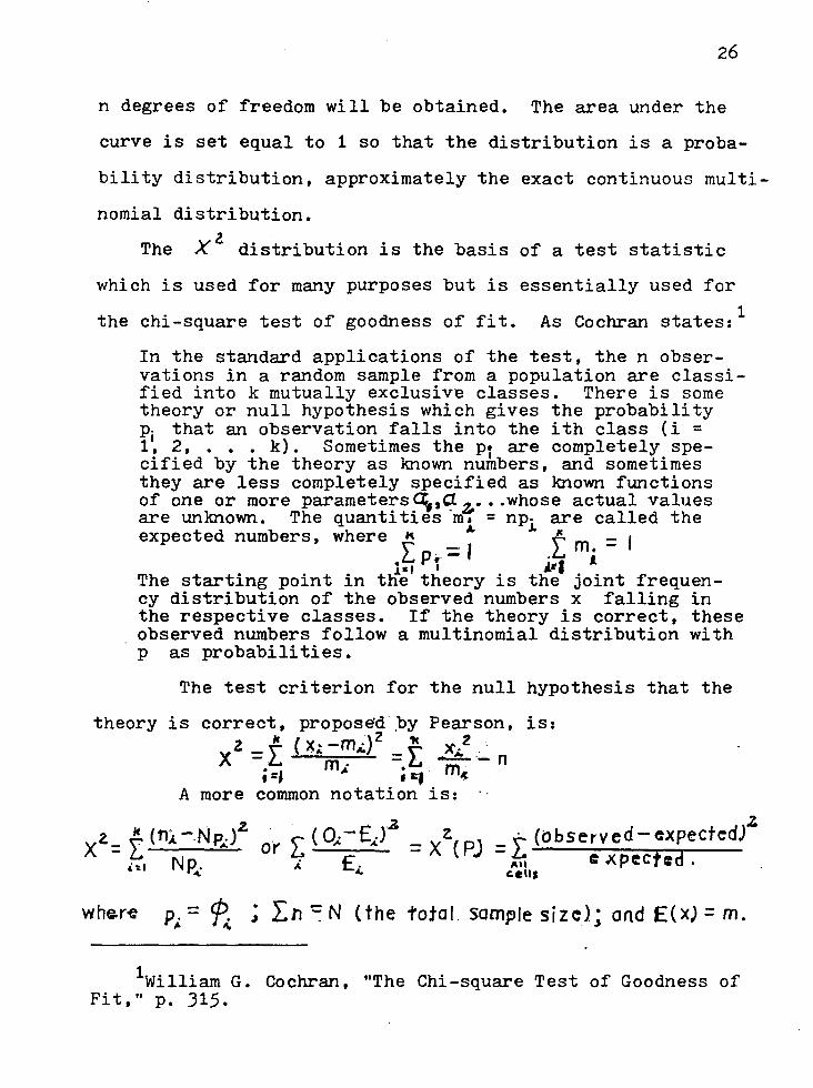
n degrees of freedom will be obtained. The area under the

curve is set equal to 1 so that the distribution is a proba­

bility distribution, approximately the exact continuous multi­

nomial distribution.

The )(2

distribution is the basis of a test statistic

which is used for many purposes but is essentially used for

the chi-square test of goodness of fit. As Cochran states: 1

In the standard applications of the test, the n obser­vations in a random sample from a population are classi­fied into k mutually exclusive classes. There is some theory or null hypothesis which gives the probability pi that an observation falls into the ith class (i = 1, 2, ••• k). Sometimes the P• are completely spe­cified by the theory as known nu~bers, and sometimes they are less completely specified as known functions of one or more parameters a,,a .z.· •. whose actual values are unknown. The quantities ·m. = np. are called the

II. J,. expected numbers, where ~< . =I [ m. = 1

Th t t . · t · tn1~ tPhr · thi~a · '. t f e s ar 1ng po1n 1n e eory 1s e J01n requen-cy distribution of the observed numbers x falling in the respective classes. If the theory is correct, these observed numbers follow a multinomial distribution with p as probabilities.

The test criterion for the null hypothesis that the

theory is correct, propose~·py Pearson, is:

X2 = t (X~ ;~.i) = E z ~· -n

i =J ,. ; ~ m~

A more common notation is:

whs.re P;. = ~ ; l:n -=: N (the total somple size); and E( x) = m.

1william G. Cochran, "The Chi -square Test of Goodness of Fit," p. 315.

27

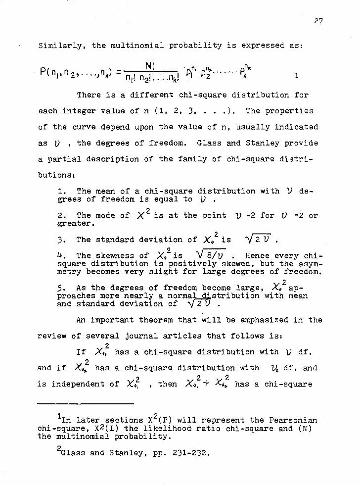
Similarly, the multinomial probability is expressed as:

P _ N! · n, n An"' ( n.l , n 2. ~ • · • • J n k) - n 1 n 1 n 1 P, Pi· · · · · · · k

I· 2· • · · · k· . l

There is a different chi-square distribution for

each integer value of n (1, 2, J, ... ). The properties

of the curve depend upon the value of n, usually indicated

as V , the degrees of freedom. Glass and Stanley provide

a partial description of the family of chi-square distri­

butions:

1. The mean of a chi-square distribution with V de­grees of freedom is equal to V •

2. The mode of X 2 is at the point V -2 for V =2 or greater.

J. The standard deviation of x_/· is Y2'V. 4. The skewness of X~2 is V 8/V • Hence every chi­square distribution is positively skewed, but the asym­metry becomes very slight for large degrees of freedom.

2. 5. As the degrees of freedom become large, X" ap-proaches more nearly a norma~stribution with mean and standard deviation of "V 2 V •

An important theorem that will be emphasized in the

review of several journal articles that follows is: 2

If X~, has a chi-square distribution with )) df. 2

and if x~,. has a chi-square distribution with v.t. df. and 2 2 X. 2 is independent of x~. , then X..;>, + ~~ has a chi-square

1In later sections x2(P) will represent the Pearsonian chi-square, X2(L) the likelihood ratio chi-square and (M) the multinomial probability.

2Glass and Stanley, pp. 231-2)2.

distribution with V1 + V.z. df. This theorem is used in model

fitting, partitioning, analysis of association, and other

methodologies.

28

The importance of the chi-square variate is parti­

cularly evident when one considers that the t, x2 , and F

distributions are all based on the normal distribution and

are interrelated as:

z2 t 2 - ---=-~

"~ - X}/v and F-.>- -

I

x} v

APPLICATIONS AND CRITICISMS OF

THE x2 STATISTIC

Most of the early relevant literature has to do

with the chi-square test and degrees of freedom, sample

size, the misuse of the test, and possible substitutes

for the statistic. As Cochran points out, the most com­

mon of all uses of the x2 test is for the 2 x 2 contin-

gency table, and a review of this r x c table is indica­

tive of the errors and conflicts that have prevailed for

many years. For example, in the 2 x 2 tables, Pearson

attributed 3 degrees of freedom to x2 , whereas it should

receive only 1, (r-1)(c-1). 1 Pearson made this correc-

tion at about the same time that Fisher was trying to

verify Pearson's work using the multinomial as an exact

test. 2 Dissonance of this type pervades the literature

on chi-square and depends upon the kind of tables being

considered, that is, whether one is considering a random

sample from only one population, or if two populations

are being compared, or if the two populations have fixed

marginal totals in repeated sampling. This complexity

increases as the dimensions of the contingency tables in-

1cochran, "X2 Test," p. 319, and Lancaster, "The x2 Distribution," pp. 170-178.

2Fisher, p. 96.

29

JO

crease, as demonstrated in the dissertation of R. J. McNamee

that has been previously mentioned.

The x2 test and distribution is used in many experi-

mental situations; however, the major applications are in

testing the goodness of fit, independence, and homogeneity.

Although this paper is concerned with a basic example of

goodness of fit, the one sample case, many of the problems

and concepts of the other applications are pertinent to this

research. The theoretical frequencies and the corresponding

sample size is a major consideration of most of the writers

already cited. Other concepts are the normal approximation

to the binomial, hypergeometric, and Poisson distribution,

maximum likelihood, minimum x2 , moments, and cumulants.

Lewis and Burke discuss at great length the rule

of thumb of having 5 or 10 as the expected cell frequencies.

They state: 1

Many users and would-be users of the chi-square test gain erroneous impressions from what they read about limitations on the size of theoretical frequencies. A textbook says that frequencies of less than 10 are to be avoided. This statement is often interpreted to mean not that 10 is a limiting value to be exceeded whenever possible, but that 10 is a value around which the various theoretical frequencies may fall; and if an occasional frequency happens to be as low as 4 or 5, that is all right because other frequencies will be larger than 10 and everything will average out in the end. A textbook that gives 5 as the suggested mini­mum tends to encourage the retention of impossibly small theoretical frequencies. And so does a text

1Lewis and Burke, "Use and fl!isuse of the x2 Test," pp. 486-487.

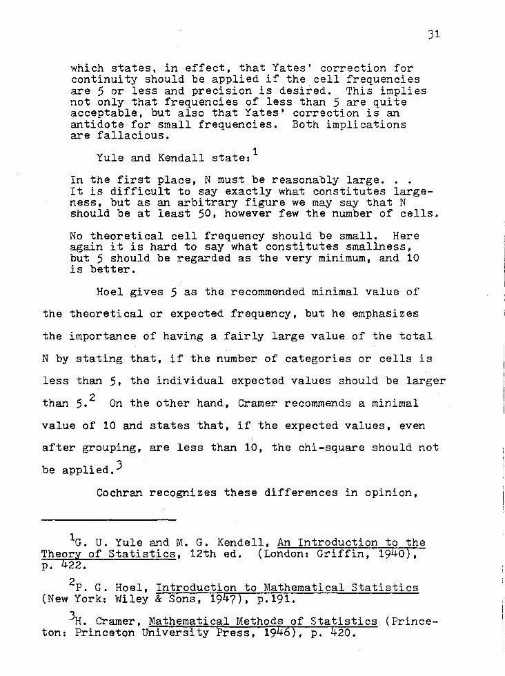
which states, in effect, that Yates' correction for continuity should be applied if the cell frequencies are 5 or less and precision is desired. This implies not only that frequencies of less than 5 are quite acceptable, but also that Yates' correction is an antidote for small frequencies. Both implications are fallacious.

1 Yule and Kendall state:

In the first place, N must be reasonably large ...

31

It is difficult to say exactly what constitutes large­ness, but as an arbitrary figure we may say that N should be at least 50, however few the number of cells.

No theoretical cell frequency should be small. Here again it is hard to say what constitutes smallness, but 5 should be regarded as the very minimum, and 10 is better.

Hoel gives 5 as the recommended minimal value of

the theoretical or expected frequency, but he emphasizes

the importance of having a fairly large value of the total

N by stating that, if the number of categories or cells is

less than 5, the individual expected values should be larger

than 5. 2 On the other hand, Cramer recommends a minimal

value of 10 and states that, if the expected values, even

after grouping, are less than 10, the chi-square should not

be applied.J

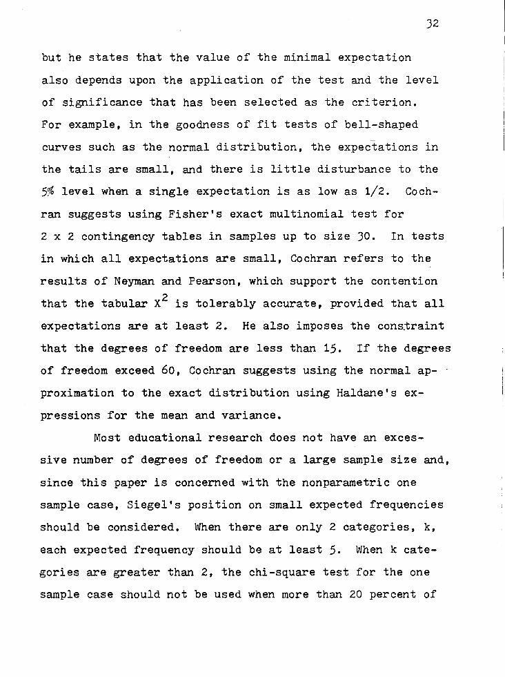
Cochran recognizes these differences in opinion,

1G. U. Yule and M. G. Kendell, An Introduction to the Theory of Statistics, 12th ed. (London: Griffin, 1940), p. 422.

2P. G. Hoel, Introduction to Mathematical Statistics (New York: Wiley & Sons, 194?), p.191.

JH. Cramer, Mathematical Methods of Statistics (Prince­ton: Princeton University Press, 1946), p. 420.

32

but he states that the value of the minimal expectation

also depends upon the application of the test and the level

of significance that has been selected as the criterion.

For example, in the goodness of fit tests of bell-shaped

curves such as the normal distribution, the expectations in

the tails are small, and there is little disturbance to the

5% level when a single expectation is as low as 1/2. Coch-

ran suggests using Fisher's exact multinomial test for

2 x 2 contingency tables in samples up to size JO. In tests

in which all expectations are small, Cochran refers to the

results of Neyman and Pearson, which support the contention

that the tabular x2 is tolerably accurate, provided that all

expectations are at least 2. He also imposes the cons~raint

that the degrees of freedom are less than 15. If the degrees

of freedom exceed 60, Cochran suggests using the normal ap­

proximation to the exact distribution using Haldane's ex-

pressions for the mean and variance.

Most educational research does not have an exces-

sive number of degrees of freedom or a large sample size and,

since this paper is concerned with the nonparametric one

sample case, Siegel's position on small expected frequencies

should be considered. When there are only 2 categories, k,

each expected frequency should be at least 5. When k cate­

gories are greater than 2, the chi-square test for the one

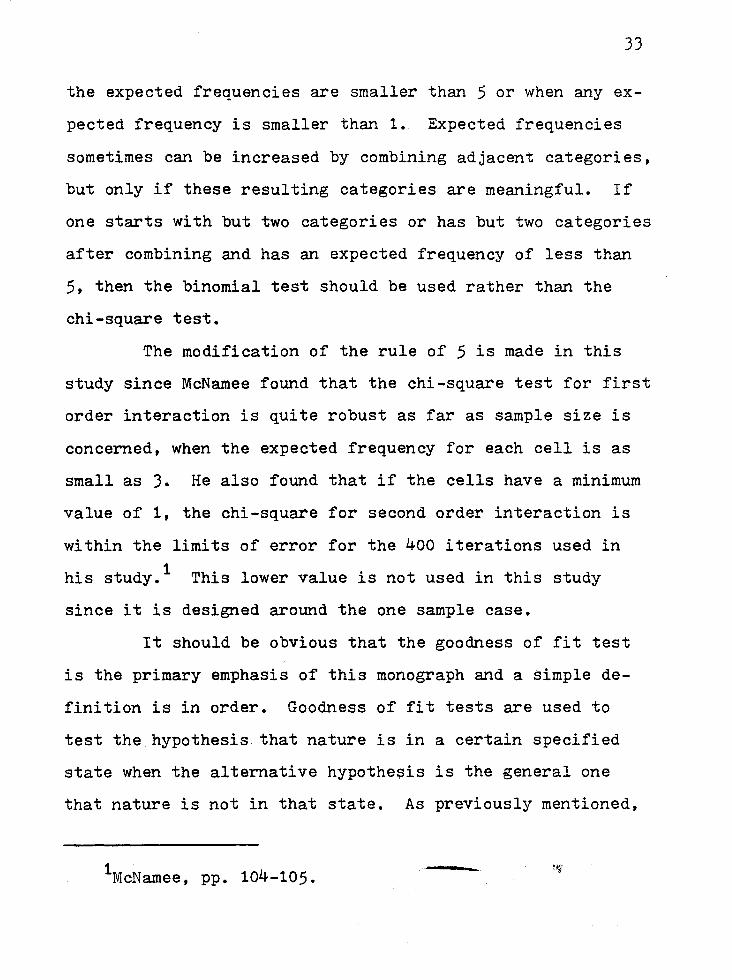
sample case should not be used when more than 20 percent of

JJ

the expected frequencies are smaller than 5 or when any ex­

pected frequency is smaller than 1. Expected frequencies

sometimes can be increased by combining adjacent categories,

but only if these resulting categories are meaningful. If

one starts with but two categories or has but two categories

after combining and has an expected frequency of less than

5, then the binomial test should be used rather than the

chi-square test.

The modification of the rule of 5 is made in this

study since McNamee found that the chi-square test for first

order interaction is quite robust as far as sample size is

concerned, when the expected frequency for each cell is as

small as J. He also found that if the cells have a minimum

value of 1, the chi-square for second order interaction is

within the limits of error for the 400 iterations used in

his study. 1 This lower value is not used in this study

since it is designed around the one sample case.

It should be obvious that the goodness of fit test

is the primary emphasis of this monograph and a simple de­

finition is in order. Goodness of fit tests are used to

test the hypothesis that nature is in a certain specified

state when the alternative hypothe$is is the general one

that nature is not in that state. As previously mentioned,

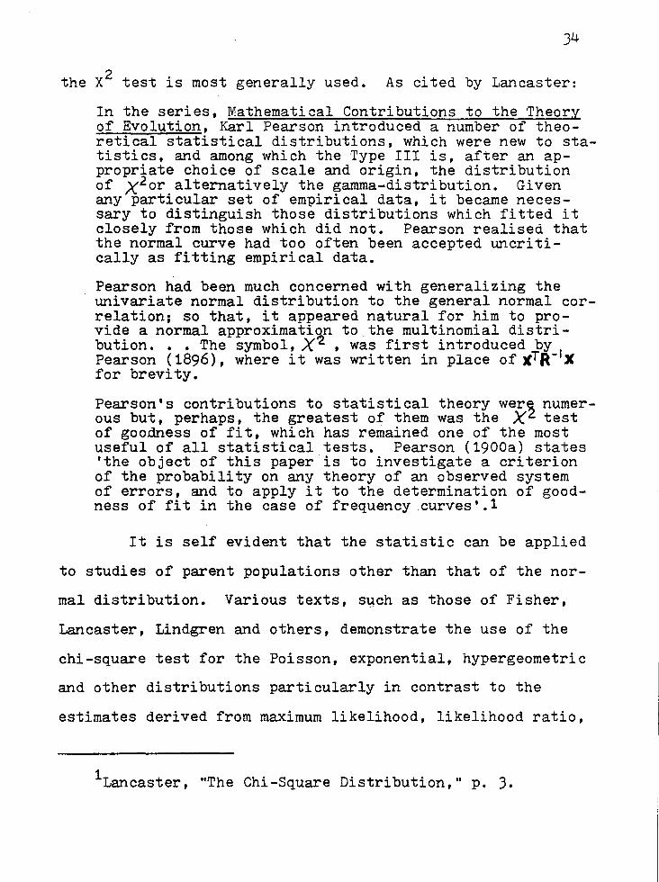
1McNamee, pp. 104-105.

34

the x2 test is most generally used. As cited by Lancaster:

In the series, Mathematical Contributions to the Theory of Evolution, Karl Pearson introduced a number of theo­retical statistical distributions, which were new to sta­tistics, and among which the Type III is, after an ap­propriate choice of scale and origin, the distribution of )(2or alternatively the gamma-distribution. Given any particular set of empirical data, it became neces­sary to distinguish those distributions which fitted it closely from those which did not. Pearson realised that the normal curve had too often been accepted uncriti­cally as fitting empirical data.

Pearson had been much concerned with generalizing the univariate normal distribution to the general normal cor­relation; so that, it appeared natural for him to pro­vide a normal approximation to the multinomial distri­bution ••• The symbol, )(~ , was first introduced by Pearson ( 1896), where it was written in place of xTR-I X for brevity.

Pearson's contributions to statistical theory wer~ numer­ous but, perhaps, the greatest of them was the X test of goodness of fit, which has remained one of the most useful of all statistical tests. Pearson (1900a) states 'the object of this paper is to investigate a criterion of the probability on any theory of an observed system of errors, and to apply it to the determination of good­ness of fit in the case of frequency curves•.l

It is self evident that the statistic can be applied

to studies of parent populations other than that of the nor-

mal distribution. Various texts, s~ch as those of Fisher,

Lancaster, Lindgren and others, demonstrate the use of the

chi-square test for the Poisson, exponential, hypergeometric

and other distributions particularly in contrast to the

estimates derived from maximum likelihood, likelihood ratio,

1Lancaster, "The Chi-Square Distribution," p. J.

35

moment and cumulant generation, and other tests.

The statistics that are derived from the sum of

the powers are based upon the concepts of moments and cum­

ulants. The first moment, m', is the arithmetic mean and

is usually written x, and it follows that the moments of

the higher powers o·f a random variable or of a distri bu­

tion are the expectations of the powers of the random

variable which has the given distribution. If X is a ran­

dom variable, the rth moment of X, usually denoted by ~; ,

"' [ , ] 1 is defined as flr = E X • It follows that the second

moment about the mean is the variance, the third moment is

a measure of the skewness, and the fourth moment is the

kurtosis.

The moments are properties resulting from a moment

generating function which is defined by letting X be a ran­

dom variable with density fx(•) • The expected value of

etx is defined as the generating function if the expected

value exists for every value of t in some interval -h< t< h;

h >o. The logarithm of the moment generating function is

defined as the cumulant function of X. The rth cumulant,

denoted by kr , is the coefficient of tr/ r! in the Taylor

1 Mood, p. 73.

J6

series expansion of the cumulant generating function. 1

This discussion of moments and cumulants is not absolutely

necessary to this current study except insofar as it may be

required in the explanation of the results and because of its

reference importance in the literature about the chi-square

distribution.

A formal presentation of the maximum likelihood

principle is beyond the scope of this paper, and is men­

tioned here briefly since it is involved in one of the sta­

tistics that is used in the calculations resulting from the

various sets of data that are generated according to selec­

ted Type III gamma distributions. Furthermore, the maximum

likelihood estimator method is the basis of rigorous proofs

used by mathematical statisticians since these estimators

meet the requirement that they are unbiased, consistent,

efficient, and sufficient. Fisher makes a point of distin-

guishing between probability and the mathematical quantity

that is appropriate for making statistical inferences among

different populations. Lindgren explains maximum likelihood

as follows:

Suppose first that the population of interest is dis­crete, so that it is meaningful to speak of the proba-bility that X=x, where X denotes a sample (X

1, ••• ,X 0 )

1 Mood, p. 80.

37

and x a possible realization(~, ..• ,xn ). This proba­bility that X=x depends on x, of course, but it also depends on the state of nature 9 which governs. As a function of 9 for given x, it is called the likelihood function:

L ( e ) = P" (X= x ) •

The principle of maximum likelihood requires first that a value 9=~ be found which furnishes the 'best explana­tion' of a given result that is observed. That is, hold­ing x fixed, we allow e to wander over the various pos­sible states of nature and select one, 9, which maxi­mizes the probability L(9) of obtaining the result ac­tually observed. Then, having found a state ~ that best explains the obsetved result x, we take the action that would be best if S really were the true state. This best action for a given state of nature is natu­rally determined by the loss function (or, equivalently, by the regret function) as that action which minimizes the loss (or regret).

Because the best explanation of a given x depends on that x, held fixed during the maximization of L(S), the minimizing 9 depends on x. It defines a function of the observations - a statistic. The rule of taking the action that minimizes l(9,a) is then a decision func­tion, an assignment of an action to each possible out­come of the sampling experiment.!

A goodness of fit test that evolves from the above

principle is that of the likelihood ratio test. For a one

sample case when the hypothesis is that nature is in a certain

specified state and the alternative hypothesis is that nature

is not in that state, the null hypothesis is:

Ho ; P 1 = 11j , • · · • and

where 1T1., •. • 7Tk are specified numbers on the interval [ 0, 1]

whose sum is 1 and k parameters p1

, ••• pk are restricted

by the condition that their sum equals 1.

1Lindgren, pp. 188-189.

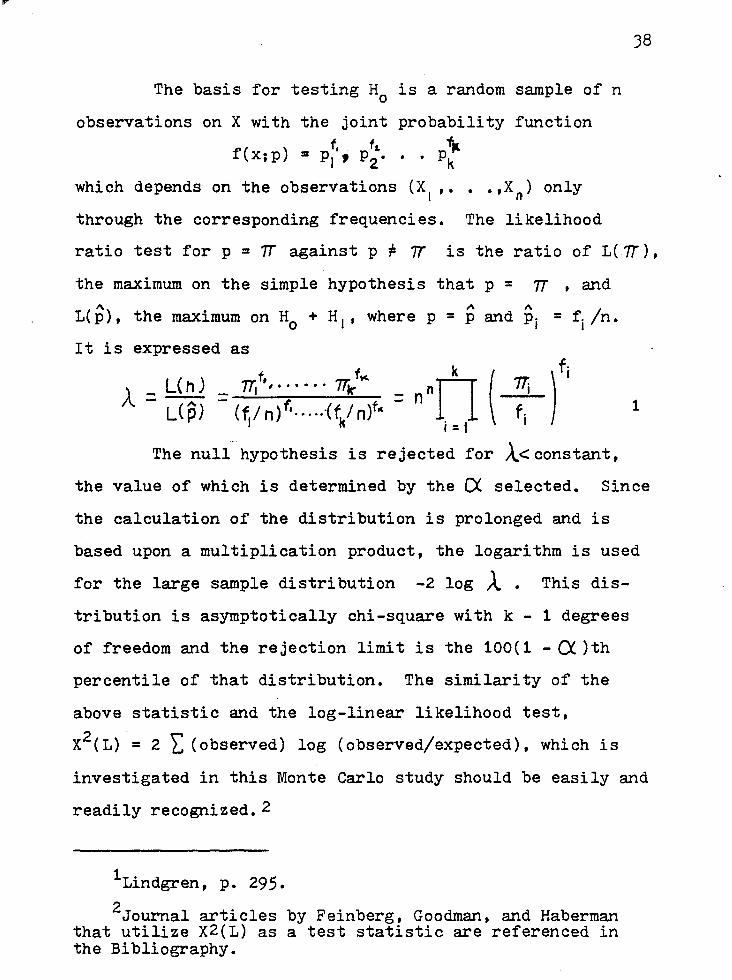
The basis for testing H0

observations on X with the joint

f( ) t, t~.

x; p :: PI ' p2.

is a random sample of n

probability function ftt

• • pk

38

which depends on the observations (X1

, ••• ,Xn) only

through the corresponding frequencies. The likelihood

ratio test for p :: 1T against p :/: Tr is the ratio of L( 1T),

the maximum on the simple hypothesis that p :: 7T , and

" 1\ " L(p), the maximum on H0

+ H1 , where p = p and pi = fi /n.

It is expressed as

L{ ) t ~ h n , · · · · · · 1r .... A - -- -~'~-=--~1'1-

- L(p) - (f,ln)f. ..... {f/n)t" = n"ri ( i i =I I

1

.. The null hypothesis is rejected for A< constant,

the value of which is determined by the CX selected. Since

the calculation of the distribution is prolonged and is

based upon a multiplication product, the logarithm is used

for the large sample distribution -2 log )l . This dis­

tribution is asymptotically chi-square with k - 1 degrees

of freedom and the rejection limit is the 100(1 -ex )th

percentile of that distribution. The similarity of the

above statistic and the log-linear likelihood test,

x2( L). = 2 'E (observed) log (observed/expected), which is

investigated in this Monte Carlo study should be easily and

readily recognized.2

1Lindgren, p. 295. 2Journal articles by Feinberg, Goodman, and Haberman

that utilize X2(L) as a test statistic are referenced in the Bibliography.

39

A brief presentation of tests that are competitive

alternatives to x2 is made because of their recur~ence in

the literature. The method of maximum likelihood consists

in multiplying the log of the number expected in each cate­

gory by the number observed, summing for all categories and

finding the value of 9 for which the sum is the positive

maximum solution of the differention of the resulting qua­

dratic equation. The method of minimum x2 is arrived at by

differentiating for the smallest positive solution resulting

from the comparison of observed with expected frequencies

and calculating the discrepancy, x2 , between them. 1

The W 2 test has been constructed and developed by

Cramer', von Mies, and Smirnov in order to avoid the group­

ing of continuous data that is necessary with x2 and still

resembles the x2 test in that the tests are not directed

against any specific alternative hypothesis. Neyman's

smooth test also postulates that the cumulative frequency

(assumed continuous) is known from the null hypothesis. If

the frequency functions which are continuous and depart in

a gradual and regular manner from the null hypothesis, the

variates will not follow a rectangular distribution in the

interval (0,1) whereas these variates would follow a rec­

tangular distribution when the deviations from the null

1Fisher, pp. 304-305, and Lancaster, pp. 136-139.

40

hypothesis are erratic or discontinuous. The x2 test is

not directed specifically at either class. 1 As it can be

noted, tests other than x2 often have certain restrictions

as to their application or information necessary to their

use. This factor coupled with the overwhelming familiarity

of users of statistical methods and the consuming audience

with the x2 results in application of this test statistic

for all but very specific problems.

1cochran, pp. 335-339.

LITERATURE BASIC TO THE PROBLEM

ERIC and Psychological Abstract searches reveal that

there has been a paucity of research regarding the chi­

square test for the one sample case, particularly for

samples randomly drawn from distributions that are not nor­

mal in form. However, it is obvious that many other chi­

square investigations are applicable to the problem that is

herein proposed.

Guenther has been actively involved in chi-square

tests for hypotheses concerning multinomial probabilities,

the power and sample size for such tests. 1 Three cases are

presented: (1) the hypothesis which specifies all the multi­

nomial probabilities, (2) the hypothesis of independence, and

(3) the hypothesis of homogeneity. He points out that if

these hypotheses are false, the statistic has approximately

a noncentral chi-square distribution with the same degrees

of freedom but also a noncentrali ty parameter A . Haynam,

Govindarajulu, and Leone have prepared tables of the non­

central chi-square distribution designed for easy solution

1T."lilliam C. Guenther, "Power and Sample Size for Approx­imate Chi-Square Tests," American Statistician, 1977, 31, pp. 83-85.

41

1 to these power problems.

42

The results of these works emphasize the large sample

size necessary for the tests to have appreciable power. An

article by Meng and Chapman further reports on the noncen­

trality parameter for r x c contingency tables. 2 Again, the

power of these tests was approximated on a large sample ba­

sis. The concept of noncentrality is introduced here only

insofar as it may be necessary to explain some of there-

sults of this study should the null hypothesis be rejected

for the small sample sizes that are used.

Categorization for this experiment has been explained

in the chapter on the statement of the problem and the means

by which the results from the random numbers generated by

the Monte Carlo study which is used and is explained in the

next chapter concerning the design. However, since questions

arise as to the effectiveness of using equal area or linear

score models, Kerlinger's rules of categorization are of

interest at this point. Categorization is another word for

partitioning, which is referred to in many articles that use

1G. E. Haynam, Z. Govindarajulu, and F. C. Leone, "Tables of the Cumulative Non-Central Chi-Square Distribu­tion," Selected Tables in Mathematical Statistics, Vol. 1, eds. H. 1. Harter and D. B. Owens, (Chicago: Markham Pub­lishing Co., 1970).

2Rosa C. Meng and Douglas G. Chapman, "The Power of Chi Square Tests for Contingency Tables," Journal of the Ameri­can Statistical Association, 1966, 61, pp. 965-975.

43

analysis of variance or multiple contingency tables as a

means of methodology.· Emphasizing that the first step in

any analysis is categorization, Kerlinger lists five rules

of categorization:

1. Categories are set up according to the research problem and purpose. 2. The categories are exhaustive. 3. The categories are mutually exclusive and inde­pendent. 4. Each category (variable) is derived from one class­ification principle. 5. Any categorization scheme must be on one level of discourse.1

Kittelson and Roscoe studied the power and robust­

ness of the chi-square and Kolmogorov statistics with both

the linear score scale and equal area models. 2 They

found that the traditional procedure for testing goodness

of fit to normal used a linear score scale model in which

the chi-square approximation of the multinomial cell limits

were defined by dividing a standard score scale into equal

parts. The criticism of this method is that the expected

frequencies in the tails of the distribution tend to be

very small with samples of reasonable size, such as n = 100

or less.

1Fred N. Kerlinger, Foundations of Behavioral Research, 2d ed. (New York: Holt, Rinehart & Winston, 1973), pp. 137-143.

2Howard M. Kittelson and John T. Roscoe, "An Empirical Comparison of Four Chi-Square and Kolmogorov Models for Test­ing Goodness of Fit to Normal" (paper presented to AERA, Chicago, 1972), pp. 1-8.

44

\Nhen the sample sizes are small, as in this experi-

ment, an alternative chi-square model has been suggested by

many authors. In these cases, the cell limits are defined

by dividing the area under the curve into equal parts - an

equal area model. Not only does this model overcome the

problem of small expected frequencies in the tails, it also

increases the power of the chi-square approximation by hav­

ing uniform expected frequencies in each division. Mann and

Wald investigated the power of the chi-square test with re­

gard to the distance of the observed and expected distribu­

tion and found that the optimum power for the goodness of

fit test for continuous distribution is achieved when the

expected frequencies are equal. 1 Williams elaborated on

their results together with useful numerical tabulations. 2

Watson suggested the equal area model for the chi­

square test of goodness of fit but also suggested· that the

number of cells should be at least ten.3 Kempthorne also

1H. B. Mann and A. Wald, "On the Choice of the Number of Class Intervals in the Application of the Chi Square Test," Annals of Mathematical Statistics, 1942, 13, pp. 306-317.

2c. A. Williams, Jr., "On the Choice of the Number and Width of Classes for the Chi Square Test of Goodness of Fit," Journal of the American Statistical Association, 1950, 45, pp. 77-86.

3G. s. Watson, "The Chi-Square Goodness of Fit Test for Normal Distributions," Biometrika, 1957, 44, pp. 336-348.

favored the equal area model, but his findings were based

in part upon a Monte Carlo study when the number of cells

(k) was set equal to the sample size (n). 1 An extensive

empirical study by Roscoe and Byars demonstrated an ac-

45

ceptable approximation with expectancies as small as one

when testing goodness of fit to uniform. 2 They found that

the approximation is not quite so good with uniform hypo-

theses, but did not examine goodness of fit to normal.

The main contribution was that the average expected fre­

quencies had to be increased for lower ex levels for uni-

form distributions and also for those distributions that

varied from the uniform; otherwise, the approximations

tended to be liberal.

Kittelson and Roscoe randomly generated ten thou­

sand uniformly distributed sets of samples for each combi­

nation of sample size and number of cells under study.

Sample sizes were 10, 20, 30, and 50. The cell sizes were

set equal to 6, 10, and 20 with the number of cells also

being set equal to 50 for samples of size 50. The null

1Kempthorne, "The Classical Problem of Inference -Goodness of Fit," Fifth Berkeley Symposium on Mathematical Statistics and Probability, 1967, 1, pp. 235-249.

2J. T. Roscoe and J. A. Byars, "An Investigation of the Restraints with Respect to Sample Size Commonly Im­posed on the Use of the Chi-Square Statistic," Journal of the American Statistical Association, 1971, 66, pp. 755-759.

46

hypothesis .was sampling from normal distribution and testing

against the normal distribution. The false hypothesis was

sampling from uniform distribution and testing from nor-

mality. The chi-square equal area models proved to be

superior to the chi-square linear score model and to both

of the Kolmogorov tests. The chi-square equal area model

was erratic with samples of size 10; however, an acceptable

approximation was achieved with all other sample sizes (n = 20, 30, and 50).

Whitney made several comparisons of various non­

parametric tests and parametric tests based on the normal

distribution and non-normal alternatives, rectangular,

double rectangular, triple rectangular, and Cauchy distri­

butions.1 With sample sizes of 5, 10, and 50, and an un­

derlying normal distribution, the normal approximation to

the binomial showed greater power than the "t" test, and

the "t" test was more powerful than the sign test. Under

the assumption of a rectangular distribution, the normal

test was considerably better than the sign test. With a

double rectangular distribution, the normal test has high

power while the sign test is of little value when there are

1D. R. Whitney, "A Comparison of the Power of Non­Parametric Tests and Tests Based on the Normal Distribu­tion Under Non-Normal Alternatives" (Ph.D. dissertation, Ohio State University, 1948).

47

only small increases in the mean but has greater power when

the increases are large.

1,11Jhen \JlJhi tney selected a triple rectangular distri-

bution with a density function that was highly peaked and

had a fair amount in the tails, the sign test had more power

than the normal or "t" tests. However, if the distribution

was flattened, the normal or "t" tests were more powerful.

With a Cauchy distribution, Whitney found the sign test

consistent, and the normal or "t" tests were inconsistent.

In his summary, Whitney states:

Alternatives in which the probability is heavily con­centrated about the mean or median favor the sign test over the normal test and the "t" test.l

This research is of a similar nature in that the

chi-square distribution is a violation of the normal assump­

tion that is often made. The chi-square test is a popular

nonparametric test statistic, and the methodology of con­

sidering the hypothesis for each quantile of the distribu-

tion is analogous to the Kolmogorov-Smirnov test statistic

with its step function and the consideration of violating

the upper and lower bounds of the selected function. De­

tails of the design of the experiment and additional review

of related literature are contained in the following chap-

ters.

1Whitney, p. 4.

CHAPTER III

DESIGN OF THE STUDY

THE ALGORITHM

The choice of an ·algorithm with which to generate

random variables from chi-square distributions using methods

to generate these variables that utilize proven techniques

and that are already known is pivotal to the study. After

review of two of the renowned volumes of Pearson and Hart­

ley1 and tables by Harter, 2 it was found and confirmed by

the IBM Research Division) that the algorithm established

by Knuth, cited below, had all the necessary attributes.

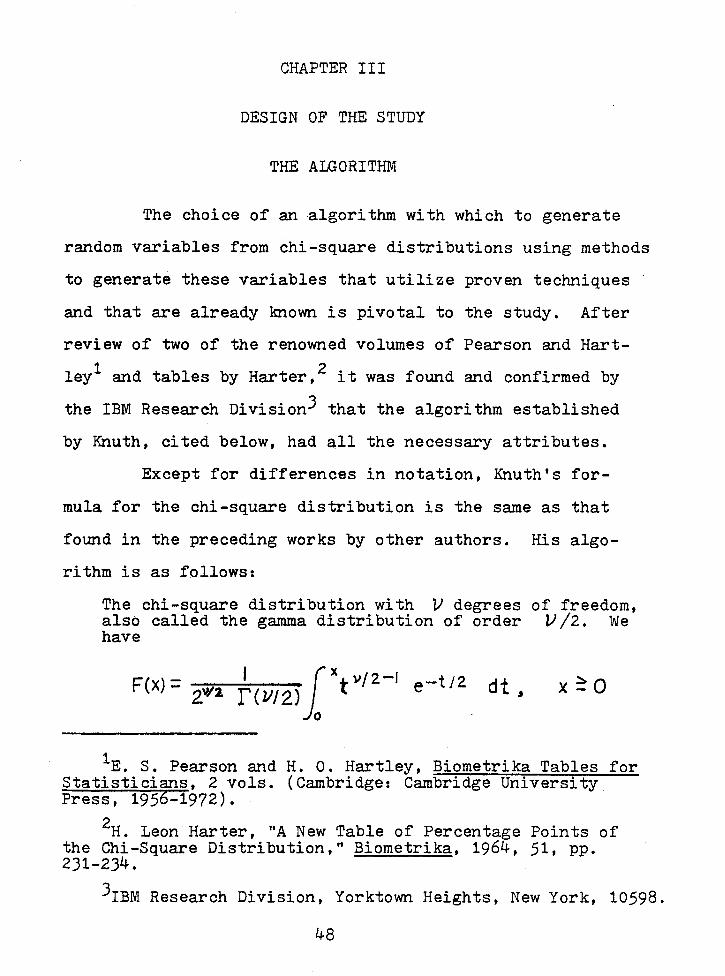
Except for differences in notation, Knuth's for­

mula for the chi-square distribution is the same as that

found in the preceding works by other authors. His algo­

rithm is as follows:

The chi-square distribution with V degrees of freedom, also called the gamma distribution of order V /2. We have

F(x)= I lxtvf2-l e-t/2 2"'2. r < vtz)

0 .

dt 1 x~O

1E. s. Pearson and H. o. Hartley, Biometrika Tables for Statisticians, 2 vols. (Cambridge: Cambridge University Press, 1956-1972).

2H. Leon Harter, "A New Table of Percentage Points of the Chi-Square Distribution," Biometrika, 1964, 51, pp. 231-234.

3IBM Research Division, Yorktown Heights, New York, 10598.

48

49

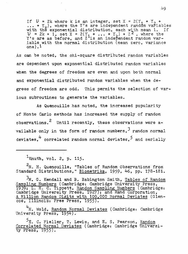
If U = 2k where k is an integer, set X = 2(Y + Y + ••• + Yk), where the y•·s are independent rand~m v~iables with the exponential distribution, each w~th mean 1. If 1J = 2k + 1, set X = 2(Y1 + ••• + Y,) + Z , where the Y's are as before, and Z is an inde~endent random var­iable with the normal distribution (mean zero, variance one) ,1

As can be noted, the chi-square distributed random variables

are dependent upon exponential distributed random variables

when the degrees of freedom are even and upon both normal

and exponential distributed random variables when the de­

grees of freedom are odd. This permits the selection of var-

ious subroutines to generate the variables.

As Quenouille has noted, the increased popularity

of Monte Carlo methods has increased the supply of random

observations. 2 Until recently, these observations were a­

vailable only in the form of random numbers,J random normal

deviates, 4 correlated random normal deviates,5 and serially

1 Knuth, vel. 2, p. 115. 2M. H. Quenouille, "Tables of Random Observations from

Standard Distributions," Biometrika, 1959, 46, pp. 178-181.

JM. G. Kendall and B. Babington Smith, Tables of Random Sampling Numbers (Cambridge: Cambridge University Press, 1939; L. H. C. Tippett, Random Sampling Numbers (Cambridge: Cambridge University Press, 1927); and Rand Corporation, A Million Random Di its with 100 000 Normal Deviates (Glen­coe, Illinois: Free Press, 1955 .

4H. Wold, Random Normal Deviates (Cambridge: Cambridge University Press, 1954),

5E. c. Fieller, T. Lewis, and E. S. Pearson, Random Correlated Normal Deviates (Cambridge: Cambridge Universi­ty Press, 1955).

50

correlated random number and normal deviates. 1 In order to

draw random observations from any distribution, it was neces-

sary to calculate the distribution function and the transfor­

mation of rectangularly distributed observations using this

function. Since these two steps could require considerable

calculations, Quenouille constructed tables that relate es-

timated values of non-normal observations to the correspond-

ing values obtained with the same observations transformed

to normality. One thousand random observations are pro­

vided from each distribution. Obviously, one thousand ran-

dom variables is an insufficient quantity for anything but

a pilot study, but Quenouille's work has been referenced

here for the researcher that might wish to write his own

program and to provide a mathematical background source.

The contents of the tables are:

xl - random normal deviates.

x2 - random rectangular deviates.

XJ - random deviates from a distribution whose log-

arithm was normally distributed.

x4 - random deviates from the exponential distri-

bution.

x5, x6, x7 - random deviates from an Edgeworth

1m. G. Kendall, "Tables of Autoregressive Series," Biometrika, 1949, 36, pp. 267-289.

51

Type A expansion with various k values.

x8 - random observations from the two-sided exponen­

tial distribution.

A_set of subroutines that are readily available and

undoubtedly come to mind first for use in the algorithm and 1 study are those of IBM- the "Scientific Subroutine Packages".

The subroutine RANDU could be used for uniformly distributed

random numbers and transformed to expo~entially distributed

numbers. The subroutine GAUSS computes normally distributed

random numbers with a given mean and standard deviation. To-

gether these operations would allow the use of the Knuth al­

gorithm for chi-square distributed random variables. How­

ever, the necessity of performing the transformations would

result in longer computer time and more lines of printout or

storage. Other subroutines from SSP that are of interest

but that can be circumvented are:

NDTR which computes y = P(x) = PROB. (X~ x) where X

is a random variable distributed normally with mean zero and

variance one.

NDTRI computes x = p-1(y) such that y = P(x) = PROB. (X-= x) where X is again a random variable distributed

1IBM, SSP ("Scientific Subroutine Packages"), Form H20-0205-J, rev. 2/14/69, pp. 68, 77, 78, 81, and 8).

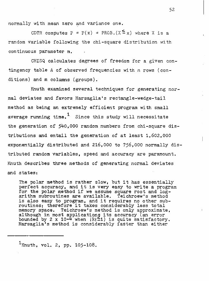
52

normally with mean zero and variance one.

CDTR computes P = P(x) = PROB.(X~x) where X is a

random variable following the chi-square distribution with

continuous parameter m.

CHISQ calculates degrees of freedom for a given con­

tingency table A of observed frequencies with n rows (con-

ditions) and m columns (groups).

Knuth examined several techniques for generating nor­

mal deviates and favors Marsaglia's rectangle-wedge-tail

method as being an extremely efficient program with small

. t' 1 average runn~ng ~me. Since this study will necessitate

the generation of 540,000 random numbers from chi-square dis­

tributions and entail the generation of at least 1,602,000

exponentially distributed and 216,000 to 756,000 normally dis-

tributed random variables, speed and accuracy are paramount.

Knuth describes three methods of generating normal deviates

and states:

The polar method is rather slow, but it has essentially perfect accuracy, and it is very easy to write a program for the polar method if we assume square root and log­arithm subroutines are available. Teichroew's method is also easy to program, and it requires no other sub­routines; therefore it takes considerably less total memory space. Teichroew's method is only approximate, although in most applications its accuracy (an error bounded by 2 x 10-4 when IR1~1) is quite satisfactory. Marsaglia's method is considerably faster than either

1 Knuth, vol. 2, pp. 105-108.

53

of the others, and like the polar method it gives essen­tially perfect accuracy. It requires square root, log­arithm, and exponential subroutines, and an auxiliary table of 100-400 constants, so its memory space require­ment is rather high; yet its speed more than compensates for this on a large computer. A program for Marsaglia's method is considerably more difficult to prepare, but a general-purpose subroutine based on Algorithm M will be a valuable part of any subroutine library.1

Just as in the case of the normal distribution,

there is an extremely fast rectangle-wedge-tail method a­

vailable for the exponential distribution based on a decom­

position of the frequency function.

Inasmuch as The McGill Random Number Package "Super­

Duper" fac.ili tated the design of this experiment to such

great extent, directions about ho~ to use the package, as

well as an off-line print-out of the source package, are in­

cluded in Appendix A. 2

The uniform number generator (which is either called

directly or else is built into the normal and exponential

generators) combines a multiplicative congruential generator

and a shift register generator. The congruential generator

uses the multiplier 69069, found after a search of millions

of multipliers to have nearly optimal lattice structure in

2, J, 4, and 5 dimensions - much better than any of the

1 Knuth, vol. 2, pp. 113-115. 2G. Marsaglia, K. Ananthanarayanan, and N. Paul, School

of Computer Science, McGill University, Montreal, Quebec, Canada, National Research Council of Canada (NRC-A7901).

54

highly touted but poorly justified multipliers used for the

past 20 years. But, even though the congruential generator

is as good as a congruential generator can be, it is still .

not good enough, and it has been combined with a shift reg-

ister generator on 32 bits (right shift 15, left shift 17).

The bit patterns produced by the two separate generators

are added as binary vectors - that is, exclusive or addition.

Combining the two generators produces a sequence with pe­

riod about 5 x 1018 •

Having established the accuracy and speed of the

methods of Marsaglia, et al, and having confirmed Ynuth's

evaluation of the randomness of th~ algorithm that will be

used in the generation of chi-square distributed random

variables, it is now fitting to discuss the Monte Carlo

methodology, the number of iterations, the calculations of

the category cut-off values, the computer program, and the

test statistics and their evaluation.

MONTE CARLO METHODOLOGY

The Monte Carlo method, often called the method of

statistical trials, is a method of solving problems of com­

putational mathematics by simulation of random quantities.

The methodology comprises that branch of mathematics which

is considered essentially experimental rather than analyt­

ical. The problems are of two types - probabilistic or

deterministic, depending upon whether or not they are con­

cerned with the behavior and outcome of random processes

or variables. 1 Kleijnen makes an interesting observation

about the use of analytical and numerical solutions:

An analytical solution uses properties known from that part of mathematics called 'analysis' which comprises differential and integral calculus. It gives a solu­tion in the form of a formula that holds for various possible values of the independent variables and para­meters. • •

A numerical solution substitutes numbers for the in­dependent variables and parameters of the model and manipulates these numbers. Many numerical techniques are iterative, i.e., each step in the solution gives a better solution using the results from previous steps ••• Two special numerical techniques are the Monte Carlo method and simulation.2

In the same vein, Hammersley states:

It should almost go without saying, if it were not so important to stress, that whenever in the Monte Carlo estimation of a multiple integral we are able to per-

1 Sobol, p. 1.

2Kleijnen, p. 5.

55

56

form part of the integration by analytical means, that part should be so performed. As in some kinds of garn-1 bling, it pays to make use of one's knowledge of form.

Electronic computers are to be credited with modern

day Monte Carlo methods, and, as Sobol points out, the

accepted birth date of the methodology is 1949, and the A-

merican mathematicians, Neyman and Ularn, are considered its

originators. 2 However, Schreider points out that histori-

cally the first example of a computation by a Monte Carlo

method is Buffon's celebrated problem of needle tossing,

which he described in 1777 in his treatise Essai d'Arith­

metigue Morale.3 This resulted in a method for computing

the quantity 1/?7. Where K is the number of times that the

dropped needles cross parallel lines on a ruled plane and

N is the number of times the needles are tossed, then ac­

cording to the Law of Large Numbers, K/N;::::, 1/ 1T.

The generation of random variables of various dis­

tribution can be obtained by transformation of independent

uniformly distributed variables as described in the preced­

ing section about the algorithm. Where Lis the number of

pairs of coordinates out of a possible N pairs, an estimate

of the computation of the probability pis based upon the

integral of the· area which can be represented by L/N~p =

~i(x) dx. The estimate of the error obviously depends on

1Hammersley and Handscomb, p. 74. 2 Sobol, p. 1.

3schreider, p. 4.

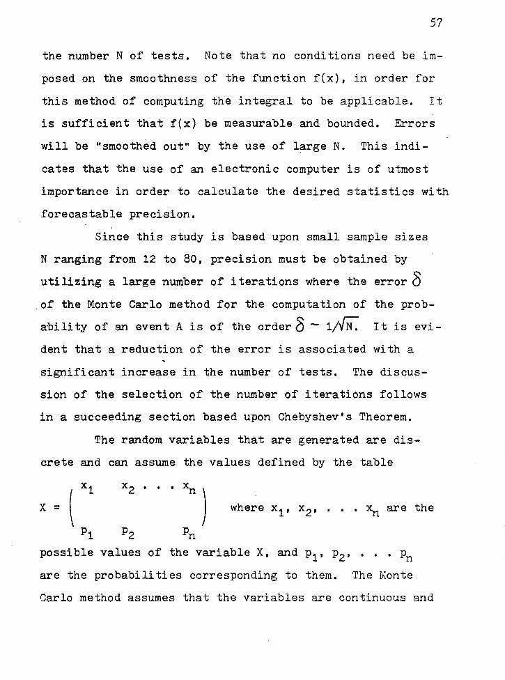
57

the number N of tests. Note that no conditions need be im-

posed on the smoothness of the function f(x), in order for

this method of computing the integral to be applicable. It

is sufficient that f(x) be measurable and bounded. Errors

will be "smoothed out" by the use of large N. This indi­

cates that the use of an electronic computer is of utmost

importance in order to calculate the desired statistics with

forecastable precision.

Since this study is based upon small sample sizes

N ranging from 12 to 80, precision must be obtained by

utilizing a large number of iterations where the error 0 of the Monte Carlo method for the computation of the prob­

ability of an event A is of the orderQ- 1/~ It is evi­

dent that a reduction of the error is associated with a

significant increase in the number of tests. The discus­

sion of the selection of the number of iterations follows

in a succeeding section based upon Chebyshev's Theorem.

The random variables that are generated are dis­

crete and can assume the values defined by the table

( x1 xz • • •

~) X = where x1 , x2 , . . • xn are the

Pt Pz Pn

possible values of the variable X, and pl' Pz' . . • Pn

are the probabilities corresponding to them. The IVIonte.

Carlo method assumes that the variables are continuous and

the probability that X lies in the arbitrary interval

(a', b') containe~ in [a, b] is equal to the integral

P(a' <:x< b') = l p(x) dx.

58

The conditions that prevail for both discrete and

continuous random variables are that the density p(x) is

non-negative and that the integral, or sum, of the density

over the whole interval is equal to 1. It should be noted

that, as the size of the intermediate intervals is reduced,

the discrete distribution approaches the continuous dis­

tribution as the limit. On the basis of a single trial

one cannot precisely predict the values that X and the cor-

' responding probability will assume. The more the trials

there are, that is, the larger the sample, the more precise

the prediction will be. '

Kleijnen and Knuth discuss the generation of ran-

dom variables for Monte Carlo studies at some great length.

Kleijnen concludes that there are no foolproof generators,

and at the present the best one seems to be the multipli­

cative generator. Since the major part of this experiment

is based upon numerical solutions and the corresponding

Monte Carlo method, Knuth's recommendation is followed, and

Marsaglia's multiplicative congruential generator with a

shift register generator has been adopted.

THE NUMBER OF ITERATIONS

The Monte Carlo methodology in this experiment is

used to approximate the probability distribution obtained

from calculating the Pearsonian and log-linear chi-square

statistics at the various quantiles represented by the cut-

off points of the various categories used in each sample set,

i.e., k = 4 to 8, and the theoretical distribution above the

ten percent level of significance. As previously stated,

the number of iterations t determines the precision of the

estimates.

The determination of the number of iterations N is

based upon a procedure used by Kavanagh1 and more recently

by McNamee. 2 Let ~2 (P) be the Pearsonian statistic and

x2(L) be the log-linear statistic calculated by the follow­

ing formulae:

x2(P) = L (observed - expected) 2/(expected) """ ....... x2(L) = 2 L (observed)log(observed/expected)

~' .... .,. McNamee's approach was that he was interested in the

90th percenti.le or less of the theoretical distribution and

1J. A. Kavanagh, "A Monte Carlo Study of the Polynomial Discriminant Method for Pattern Recognition" (Ph.D. Disser­tation, University of Minnesota, 1972), p. 26.

2McNamee, pp. 40-42.

59

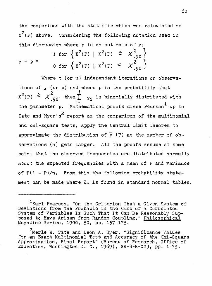
the comparison with the statistic which was calculated as

x2(P) above. Considering the following notation used in

this discussion where p is an estimate of y:

1 for { x2(P) I x2(P) .:::. x~9o} -y = p =

{ x2 (P) I x2(P) x~9o} 0 for <

Where t (or n) independent iterations or observa­

tions of y (or p) and where pis the probability that 2 ::> 2 t

60

X (P) - X. 90 , theni~ Yi is binomially distributed with

the parameter p. Mathematical proofs since Pearson1 up to

Tate and Hyer•s2 report on the comparison of the multinomial

and chi-square tests, apply The Central Limit Theorem to

approximate the distribution of y (P) as the number of ob­

servations (n) gets larger. All the proofs assume at some

point that the observed frequencies are distributed normally

about the expected frequencies with a mean of P and variance

of P(1 - P)/n. From this the following probability state-

ment can be made where z~ is found in standard normal tables.

1Karl Pearson, "On the Criterion That a Given System of Deviations from the Probable in the Case of a Correlated System of Variables Is Such That It Can Be Reasonably Sup­posed to Have Arisen from Random Coupling," Philosophical Magazine Series, 1900, 50, pp. 157-175.

2Merle W. Tate and Leon A. Hyer, "Significance Values for an Exact Multinomial Test and Accuracy of the Chi-Square Approximation, Final Report" (Bureau of Research, Office of Education, Washington D. C., 1969), BR-8-B-023, pp. 1-75.

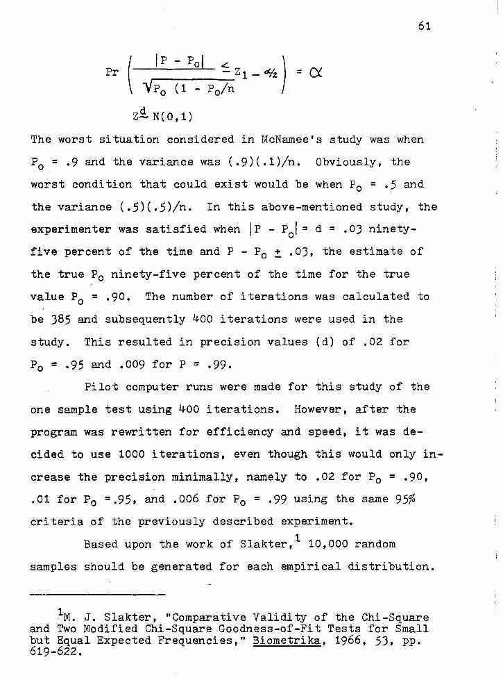
61

Pr - Z1- DCfz. = Cf. ( I P - Pal ~ )

VP0 ( 1 - P0 /n

z£. N( o, 1)

The worst situation considered in McNamee's study was when

P0 = .9 and the variance was (.9)(.1)/n. Obviously, the

worst condition that could exist would be when P0 = .5 and

the variance (.5)(.5)/n. In this above-mentioned study, the

experimenter was satisfied when jP - P0

1 = d = .03 ninety­

five percent of the time and P - P0 ! .03, the estimate of

the true P0 ninety-five percent of the time for the true

value P0 = .90. The number of iterations was calculated to

be 385 and subsequently 400 iterations were used in the

study. This resulted in precision values (d) of .02 for

P0 = .95 and .009 for P = .99.

Pilot computer runs were made for this study of the

one sample test using 400 iterations. However, after the

program was rewritten for efficiency and speed, it was de­

cided to use 1000 iterations, even though this would only in­

crease the precision minimally, namely to .02 for P0 = .90,

.01 for P0 =.95, and .006 for P0 = .99 using the same 95%

criteria of the previously described experiment.

Based upon the work of Slakter, 1 10,000 random

samples should be generated for each empirical distribution.

1M. J. Slakter, "Comparative Validity of the Chi-Square and Two Modified Chi-Square Goodness-of-Fit Tests for Small but Equal Expected Frequencies," Biometrika, 1966, 53, pp. 619-622.

62

Similar calculations for this experiment would have meant

ten times as many computations as were used and the genera­

tion of over 23,580,000 random variables. Tate and Hyer 1

used 65,536 sets of outcomes for the relatively simple multi­

nomial distribution, N·= 8, k = 4 and the qbequal. Their

total grant required in excess of 8,000,000 sets of out­

comes. It is self evident that there is insufficient time

or money to extend this study to a like scope.

1Tate and·Hyer, p. 5.

CATEGORIZATION AND PROGRAMMING

The arguments for the use of the equal area model for

the chi-square test of goodness of fit were discussed exten­

sively in the previous chapter, pages 42-46. The samples of

random variables that are generated in this study are cate­

gorized accordingly. The only difficulty that arises in

such categorization is the establishment of the chi-square

category cut-off_points for many of the various percentiles

that are not generally tabulated. Although interpolation

of values of X 2. is explained in BTS 1, 1 the procedures

suggested in BTS 22 are used since this volume includes

many tabulations calculated by Harter,3 which are more com­

prehensive than previous tabulations in that the tables are

entered with V and P, rather than Q; include additional en­

tries for P; and have eight significant figures for low

values of V and P rather than the usual six significant

figures.

Where 3-decimal accuracy is adequate, linear inter-

polation is usually sufficient and particularly where v < 30.

However, for greater accuracy, and in line with established

1Pearson and Hartley, BTS 1, pp. 13-16. 2Pearson and Hartley, BTS 2, pp. 140-142 and pp. 382-385.

)Harter, p. 234.

63

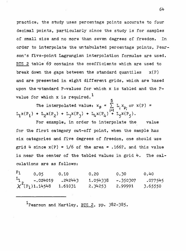
64

practice, the study uses percentage points accurate to four

decimal points, particularly since the study is for samples

of small size and no more than seven degrees of freedom. In

order to interpolate the untabulated percentage points, Pear-

son's five-point Lagrangian interpolation formulae are used.

BTS 2 table 69 contains the coefficients which are used to

break down the gaps between the standard quantiles x(P)

and are presented in eight different grids, which are based

upon the•standard P-values for which xis tabled and the P­

value for which xis required. 1 5

The interpolated value: xp = L i=l

L1x(P1) + L2x(P2 ) + L3x(P

3) + L4x(P4 ) +

For example, in order to interpolate the value

for the first category cut-off point, when the sample has

six categories and five degrees of freedom, one should use

grid 4 since x(P) = 1/6 of the area= .1667, and this value

is near the center of the tabled values in grid 4. The cal­

culations are as follows:

0.10 .242443

1.61031

0.20 1.054338 2.34253

0.30 -.350307 2.99991

1Pearson and Hartley, BTS 2, pp. 382-385.

0.40

.077545 3.65550

r

65

Summing the products Li )( 2{Pi), it is found that

X 2. ( .16 I 5) = 2. 0651897. Subtracting this from X 2(. 2015)

= 2.34253, dividing the difference by 400, multiplying this

quotient by 67, and adding the product to X 2( .16J 5) re-

. 2 sul t in the linear interpolation for X ( .166715) = 2. 112.

2 This was checked by calculated X (.17f5) and interpolat-

ing downward to .1667 with comparable results.

With the algorithm selected and with the categori-

zation process established, the succeeding steps in the de-

sign are to write an assembler-fortran program to generate 2 2 the random variables, calculate X (P) and X (L) for the var-

ious sample sets, and then refine the program for speed and

ease of evaluation. First, the fortran subroutine for cal­

culating the Pearsonian chi-square probabilities, x2(P), was

adapted from the SPSS package, and fortran statements for

the calculation of the log-linear chi-square probabilities,

x2(L), were appended to the random number generator that has

been previously discussed. Part of a sample run of 40 iter­

ations is given in Appendix B and demonstrates how lengthy

and time consuming the basic design could be, while also

showing how the algorithm is used for a chi-square distri­

bution with four degrees of freedom and expected frequencies

of three. Column one consists of the Y1 random numbers that

are generated from an exponential distribution, column two

consists of the Y2 variables, and column three is the de­

sired chi-square random variable which is twice the sum of

66

Y1 and Y2 • The cell frequencies are displayed along with

the Pearsonian and the log-linear chi-square values and the

apropos probabilities. It should be noted that this sample

of 40 iterations required 986 lines, evidence that the pro­

gram had to be condensed for 1000 iterations of the fifteen

sample sets that are studied.

Appendix C shows the output of an intermediate stage

in the evolution of the final program. This sample run is

for a chi-square distribution having seven degrees of free­

dom and expected cell frequencies of three. For the sake of

brevity, only the fortran statements and some of the output

is reproduced in this appendix, which displays how the pro­

gram branches to X = 2(Y1 + ••• Yk) for distributions hav­

ing an even number of degrees of freedom or branches to

X = 2(Y1 + Yk) + z2 for odd numbered degrees of freedom. As

before, the Pearsonian and log-linear chi-square values and

probabilities are printed. When the log-linear statistic is

indeterminate because of a zero cell frequency, this fact is

flagged by the printing of a series of asterisks.

Appendix D is an example of the final condensed ver­

sion of the program that was evolved and part of the output

when 1000 iterations were used for each sample set. It

should be noted that the intermediate calculations are not

printed and that the output is sorted according to the prob­

abilities of the Pearson test statistic. This procedure

facilitates the tabulation and comparison of x2(P) and

x2 (L).

67

Calculations by the use of an electronic hand cal­

culator were made of randomly selected sample sets at each

stage of the programming evolution to verify the accuracy of

the computer work. In addition, the nonparametric subroutine

of SPSS VII for one case samples was used for further proof

of the program. A -single example of this is shown in Appen­

dix E and demonstrates the value of the program that was de­

signed when many cases must be studied and speed and effi­

ciency are of utmost concern • •

EVALUATION

The primary hypothesis:

Ho : Pl = Pot

Pz = Paz

Pk = Pok

will be evaluated for x2(P) and x2(L) by tabulating the fre-

quencies that appear within the equal area proportions for

both test statistics when the number of categories were se­

lected a priori from 4 to 8 and the expected cell frequencies

were 3, 5, and 10.

For example, when K = 4, the hypothesized propor­

tions falling within each category are 25 percent. Using

1000 iterations, 250 sample sets should fall within each

category. However, when zero cell frequencies occur, x2(L)

is indeterminate, as can be recognized from the test statis­

tic: x2 (L) = 2 L(observed)log(observed/expected). ~~en

this occurs, the number of indeterminate iterations will

be noted on the tabulation and the percentages adjusted

accordingly. The percentage of error that occurs will also

be displayed for both test statistics. Since 10 percent is

68

69

usually the criteria of goodness of fit when a researcher

is "model fitting", as in ANOVA, ANOCOVA, etc., the null

hypothesis will be accepted if the experimental frequencies

are within this 10 percent limit. In order to identify the

effect of small sample size, the tabulations will be pre­

sented separately for each K category and the three expec­

ted frequencies, E(x) = J, 5, and 10.

For each N and K, where q' = 1/K, the chi-square

probabilities for x2 (P) and x2(L) will be tabled in the

.005-.009, .010-.050, and .051-.100 regions since these re-

gions are the ones most often used in making statistical in­

ferences in the one sample case. These tabulations will

also show the exact multinomial probabilities that are a-

vailable from the Tate and Hyer study previously noted. Ex­

cept for the special case of the binomial distribution,

there had previously been no tables of the multinomial. The

reason for this is that there are too many parameters in the

general case to permit construction of manageable tables,

and the expansion of the multinomial is long and laborious

for all but small N. However, in the case of the equal area

model being studied, the cf:> are equal, just as in the Tate

and Hyer 1 study, and the size of the tables and the labor

is greatly reduced. This is particularly true if the cal­

culations are made using logarithms and log factorials when

1Tate and Hyer, pp. 1-8 and pp. 25-75.

70

computing the multinomial probability of an outcome. Tate

and Hyer used a digital computer program that was written

by David 1. March1 for a CDC 6400 computer to further re­

duce the complexity of the procedures.

Since the Tate study of the multinomial distribution

was limited to N of JO or less and 1' of 1/7 or more, a com­

plete comparison of the multinomial probability of P(M) and

x2 (P) and x2 (L) is possible for only part of this study •

•

1David 1. March, Multin Program, 1968, Lehigh Univer­sity Computing Center, Bethlehem, Pa.

CHAPTER IV

RESULTS OF THE STUDY

INTRODUCTION

This chapter presents the results of the study

which were derived using Monte Carlo methodology to gener­

ate random numbers from gamma distributions of order V/2,

which are Pearson's chi-square distributions with V de­

grees of freedom. This decision was based on the desire

to verify Siegel's claim that nonparametric techniques are

distribution free, whereas researchers most often generate

their random variables from uniform or normal distribu­

tions·. By varying the degrees of freedom from 3 to 7, dis­

tributions of varying measures of skewness were generated.

Sample size was manipulated by using expected cell frequen­

cies of 10, 5, and 3.

As originally programmed, see Appendix B, this re­

search required 1,080,000 random numbers constructed from

1,602,000 exponentially and 756,000 normally distributed

random variables and necessitated 745,500 lines of computer

output and 3 hours 55 minutes 52.5 seconds of CPU time,

even though the efficient McGill Random Number Package

"Super-Duper" was used. The intermediate program, shown as

Appendix C, cut the CPU time but increased the lines of out-

71

72

put to over 4,000,000. The program that was finally evolved

required only 42,345 lines of output and 41 minutes 38.9

seconds of CPU time, a drastic reduction. A sample of this

program is displayed as Appendix D.

The efficiency of the Monte Carlo program made it

possible to examine various one sample cases with expected

values of 10, 5, and 3 in each cell. These numbers were

proposed in many articles reviewed in CHAPTER II and will

be discussed further in the following sections, particu­

larly those on the use of Fienberg's x2(L) and the equal

area models with categories of 4, 5, 6, 7 and 8, wherein

the total sample size is restricted, as noted in the STATE-

MENT OF THE PROBLEM.

The rationale for the use of ex regions rather

than point estimates is explained in the section on the

goodness of fit. The results obtained from the use of Pear­

son's chi-square, x2(P), the log-linear likelihood ratio,

x2(L), and the multinomial, (M), for these regions are re­

ported as a function of the expected cell frequencies, E(x),

and the number of categories, k. Generally, x2(P) is as

desirable a test statistic as the multinomial (M). How-

ever, the deviations that do exist have interesting impli­

cations which will be discussed in the pertinent sections.

X 2 ( P) OR X 2 ( L) FOR SrJIALL SAMPLES

Since so little research has been reported re-

garding the chi-square test for the one sample case, exam­

ples of the one sample case and the constraints imposed in

this study are reiterated to differentiate this experiment

from many other chi-square investigations. Siegel explains

the function of the chi-square one sample test as follows:

Frequently research is undertaken in which the re­searcher is interested in the number of subjects, ob­jects, or responses which fall in various categories. For example, a group of patients may be classified ac­cording to their preponderant type of Rorschach re­sponse, and the investigator may predict that certain types will be more frequent than others. Or children may be categorized according to their most frequent modes of play, to test the hypothesis that these modes will differ in frequency. Or persons may be categorized according to whether they are 'in favor of', 'indif­ferent to', or 'opposed to' some statement of opinion, to enable the researcher to test the hypothesis that these responses will differ in frequency.

The x2 test is suitable for analyzing data like these. The number of categories may be two or more. The tech­nique is of the goodness-of-fit type in that it may be used to test whether a significant difference exists between an observed number of objects or responses fall­ing in each category and an expected number based on the null hypothesis.

In order to be able to compare an observed with an ex­pected group of frequencies, we must of course be able to state what frequencies would be expected. The null hypothesis states the proportion of objects falling in each of the categories in the presumed population. That is, from the null hypothesis we may deduce what are the expected frequencies.l

1siegel, pp. 42-43

73

74

A key phrase is 'the presumed population'. Much of the lit-

erature that has been reviewed is based upon sampling from

uniform or normal populations although the seed for this re-

search was Fienberg's statement that, for small samples, it

is not clear whether x2 (P) or x2 (L) is the superior statis-

tic, and that study was based upon sampling from Poisson

distributions. 1

As Fienberg explained, the same maximum likelihood

estimates for the expected cell counts for log-linear mod­

els can be obtained under a variety of different sampling

procedures. The most simple such sampling procedure which

can be assumed is that one where the observed cell counts

have independent Poisson distributions with the expected

counts as their means. However, since this experiment is

concerned with small sample sizes and small expected cell

frequencies, the basic assumption was made to sample from

skewed chi-square distributions of various degrees of free­

dom.

In support of Cochran, 2 Siegel states that "The

chi-square test for the one sample case should not be used

when more than 20 percent of the expected frequencies are

smaller than 5 or when any expected frequency is smaller

than 1."3 McNamee showed that the chi-square test for

1Fienberg, pp. 421-425. 2cochran, "X2 Test," p. 319.

3siegel, p. 46.

75

first order interaction is quite robust with expected values

as small as 3. 1 This conclusion and the well-known rules of

5 or 10 decided what expected values would be covered in this

study.

The results of 1000 iterations for the 15 different

combinations of 5 categories and 3 expected frequencies are

displayed in Table 1 on the following pages, listed in as­

cending order of k categories with q'= 1/k and E(x) = 10, 5,

and 3. The theoretically expected frequency for each cate­

gory is 1000/k. The observed frequency for each equal pro­

portion is listed along with the percentage deviation from

the theoretical frequency,% e, for X2(P) and x2(L). The

frequencies of x2 (L) that are indeterminate, Indet, are

listed for the corresponding proportions. The frequencies

of chi-square probabilities generated from a normal distri­

bution and the deviation from the theoretical frequencies

are listed as f Gauss and % e. This latter sampling pro­

cedure will be discussed in the following section, EVALU-

ATION OF THE HYPOTHESIS OF EQUAL PROPORTIONS.

Since the .10 level is the usual ex level for good-

ness of fit tests, it has been selected as the criterion

for the comparison of the two test statistics, x2 (P) and

x2 ( 1) • For example, when K = 4, ¢= 1/4, E(x) = 10, and

N = 40, the deviations for the 4 categories are less than

1 McNamee, p. 104.

76

10 percent, as shown in Table 1, and x2(P) or x2(L) result

in similar decisions of inference or hypothesis testing for

the one sample case. Both statistics support the null hypo­

thesis that the samples came from chi-square populations.

Likewise, when K = 5, q) = 1/5, E(x) = 10, and N = 50, an

experimenter would be likely to use x2(P) or x2(L). Only

when K = 4 and E(x) = 5 and when K = 6 and E(x) = 10, does

x2(L) display a better fit to the sampled chi-square dis­

tributions than x2 (P), and this could be due to experiment-

wise error since 45 sample sets were generated.

The most obvious disadvantage to the use of x2(L)

for small samples is the increasing number of the statistic

that are more and more indeterminate as the number of cate-

gories are increased, and the expected frequencies are de­

creased. The pattern of the number of these indeterminate

test statistics also reflects the skewness and kurtosis of

the populations since the categories with the higher propor­

tions, i.e., the right-hand tail, have increasing frequencies

of indeterminate results.

The number of zero observations that are encountered

in the higher probabilities of the chi-square and the arith­

metic of the test statistic, x2(L) = 2 L (observed)log(ob­

served/expected), portends that many calculations would be

indeterminate since the logarithm of zero divided by anum­

ber is indeterminate. In the case of contingency tables,

this effect can be negated to a large degree by transposing

77

rows or columns, as in the study by McNamee. 1 A point not

emphasized is that such transposition changes the identifi-

cation of the corresponding interactions. Fienberg, Goodman,

Haberman and others utilizing transposition modify the models

to reflect the alteration or deletion of some interactions. 2

The rejection of x2(L) for use in one sample cases does not

detract from Fienberg's use in the analysis of multidimen­

sional contingency tables, since x2 (L) can be used in the se­

lection of suitable models, via an iterative technique of

partitioning.

Further reference to the use of x2 (P) and x2(L) is

made in a succeeding section in which the statistics are com­

pared to the exact multinomial in three ex regions from .005

to .100 with the implications for goodnes~ of fit.

1 McNamee, p. 66 2Fienberg, pp. 426-431.

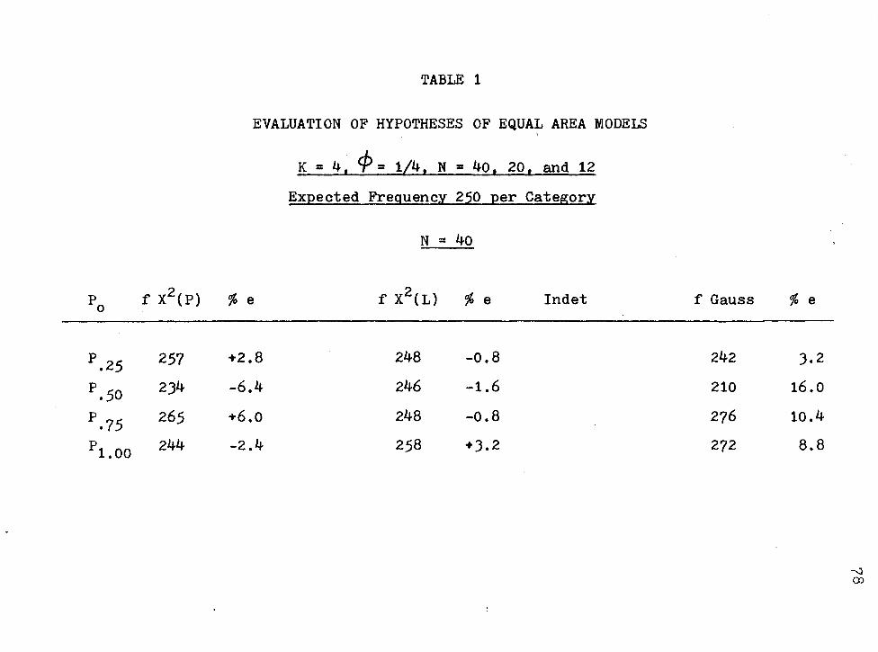
TABLE 1

EVALUATION OF HYPOTHESES OF EQUAL AREA MODELS \

K = 4 I cp = 1/4 I N = 40 I 20 1 and 12

Expected Freguency 250 per Category

N = 40

Po f x2 (P) % e f x2 (L) % e Indet

P.25 257 +2.8 248 -0.8

P.5o 234 -6.4 246 -1.6

P.75 265 +6.0 248 -0.8

Pl.OO 244 -2.4 258 +).2

f Gauss

242

210

276

272

% e

).2

16.0

10.4

8.8

-....} ())

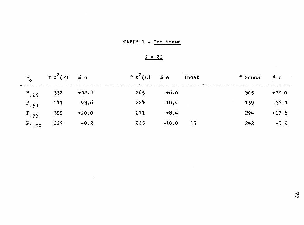
TABLE 1 - Continued

N = 20

Po f x2(P) % e f X2(L) % e

P.25 332 +32.8 265 +6.0

P.50 141 -43.6 224 -10.4

P.75 300 +20.0 271 +8.4

P1.00 227 -9.2 225 -10.0

Indet f Gauss

305

159

294

15 242

% e

+22.0

-36.4

+17.6

-3.2

---J \.()

...

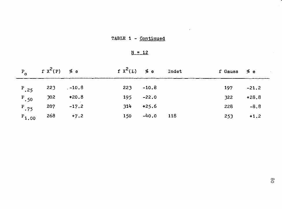
TABLE 1 - Continued

N = 12

Po r x2(P) % e f x2( L) % e

P.25 22.3 . -10.8 22.3 -10.8

P.50 .302 +20.8 195 -22.0

P.75 207 -17.2 .314 +25.6

P1.00 268 +7.2 150 -40.0

Indet f Gauss

197

.322

228

118 25.3

% e

-21.2

+28.8

-8.8

+1.2

())

0

"'""'!

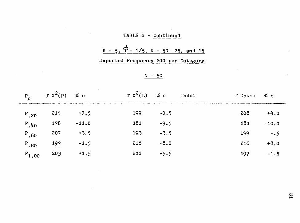
Po r x2(P) % e

P.20 215 +7.5

P.4o 178 -11.0

P.6o 207 +).5

P.8o 197 -1.5

P1.00 20) +1.5

TABLE 1 - Continued

K = 5, ~= 1/5, N = 50, 25, and 15

Expected Frequency 200 per Category

N = ,50

r x2(L) % e Indet

199 -0.5

181 -9.5

19) -).5

216 +8.0

211 +5.5

f Gauss

208

180

199

216

197

% e

+4.0

-10.0

-.5

+8.0

-1.5

co p

p f x2(P) % e 0

P.20 20? +).5

P.4o 116 -42.0

P.6o 262 +)1.0

P.8o 196 -2.0

P1.00 219 +9.5

TABLE 1 - Continued

N = 25

f x2(L) % e

184 -8.0

160 ·-20 .o

215 +?.5

204 +2.0

218 +9.0

Indet f Gauss

2)2

12?

244

190

19 207

% e

+16.0

-)6.5

+22.0

-5.0

+).5

(X) l\)

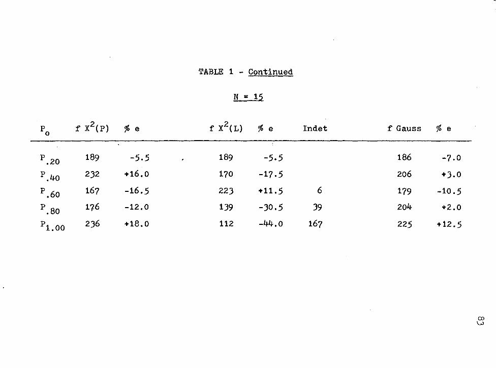
TABLE 1 - Continued

N = 15

p r x2(P) % e r x2(L) % e 0

P.20 189 -5.5 . 189 -5.5

P.4o 2.32 +16.0 170 -17.5

P.6o 167 -16.5 22.3 +11.5

P.80 176 -12.0 1.39 -.30.5

P1.00 2.36 +18.0 112 -44.0

Indet f Gauss

186

206

6 179

.39 204

167 225

% e

-7.0

+.3. 0

-10.5

+2.0

+12.5

()) \..;J

"lllll

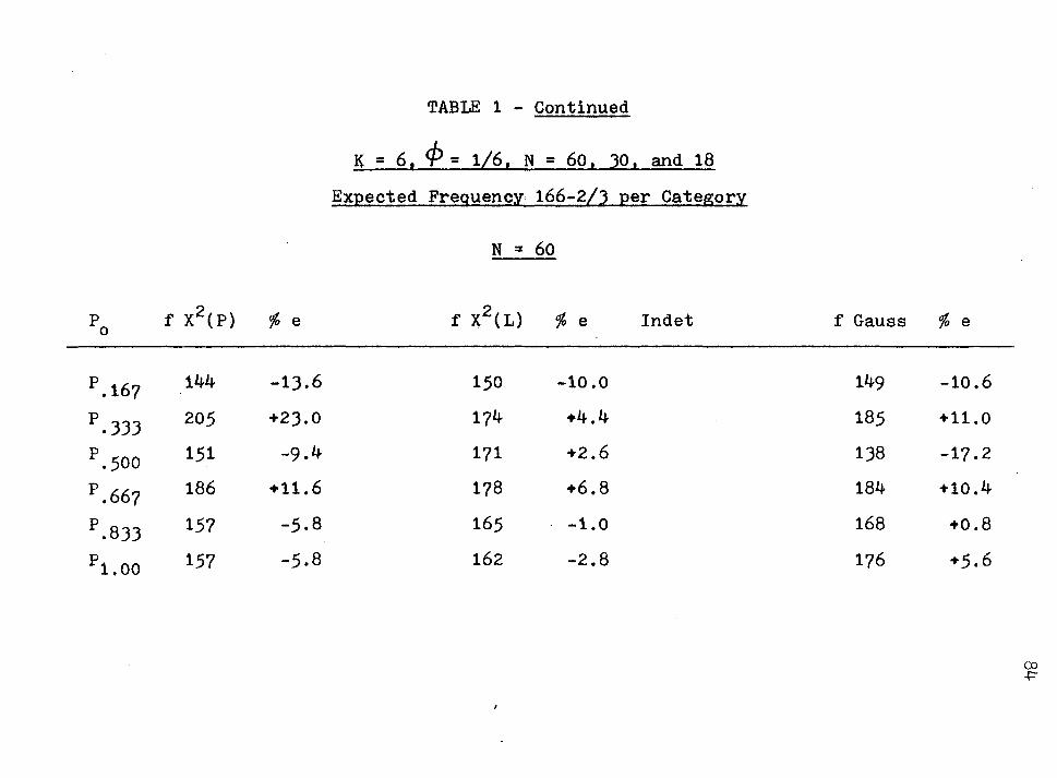
p r x2( P) % e 0

P.167 144 -13.6

P.333 205 +23.0

P.500 151 -9.4

P.667 186 +11.6

P.833 157 -5.8

P1.00 157 -5.8

TABLE 1 - Continued

I< = 6 1 cp = 1/6 1 N = 60 1 30 1 and 18

Expected Frequency, 166-2/J per Category

N = 60

r x2( L) % e Indet

150 -10.0

174 +4.4

171 +2.6

178 +6.8

165 -1.0

162 -2.8

f Gauss

149

185

138

184

168

176

% e

-10.6

+11.0

-17.2

+10.4

+0.8

+5.6

(Xl {:"

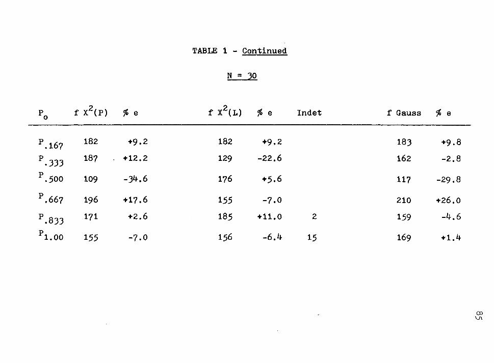
TABLE 1 - Continued

N = 30

Po f x2(P) % e f x2(L) % e

P.167 182 +9.2 182 +9.2

P.))J 187 +12.2 129 -22.6

P.500 109 -)4.6 176 +5.6

P.667 196 +17.6 155 -7.0

P.8)) 171 +2.6 185 +11.0

P1.00 155 -7.0 156 -6.4

Indet f ,Gauss

183

162

117

210

2 159

15 169

% e

+9.8

-2.8

-29.8

+26.0

-4.6

+1.4

(X)

\..rl

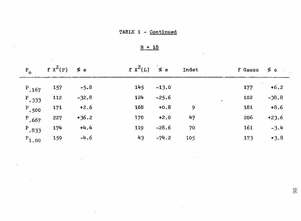
TABLE 1 - Continued

N = 18

Po r x2(P) % e r x2(L) % e

p~167 157 -5.8 145 -1.3.0

P.J.3.3 112 -.32.8 124 -25.6

P.500 171 +2.6 168 +0.8

P.667 227 +)6.2 170 +2.0

P.8.3.3 174 +4.4 119 -28.6

P1.00 159 -4.6 4.3 -74.2

Indet f Gauss

177

102

9 181

47 206

70 161

105 17.3

% e

+6.2

-.38.8

+8.6

+2).6

-.3.4

+ .3. 8

(X)

0'\

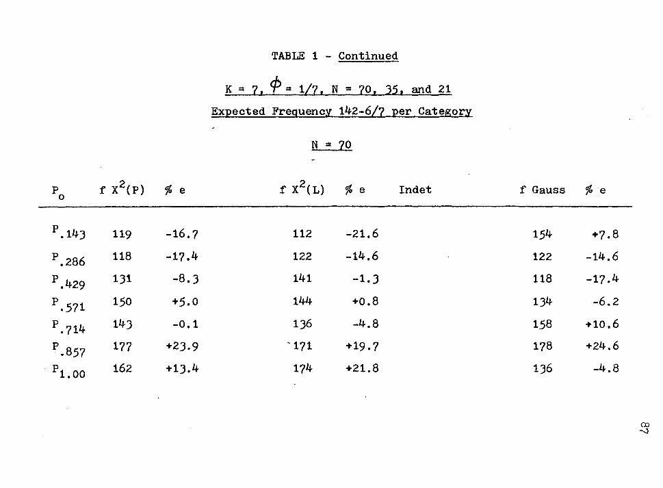
Po r x2(P) % e -

p .14) 119 -16.7

P.286 118 -17.4

P.429 1)1 -8.)

P.571 150 +5.0

P.714 14) -0.1

P.857 177 +2).9

P1.00 162 +1).4

TABLE 1 - Continued

K = 7, ¢> = 1/7, N = ?O, 35, and 21

Expected Frequency 142-6/7 per Category

N = 70

f x2(L) % e Indet

112 -21.6

122 -14.6

141 -1.3

144 +0.8

1)6 -4.8

'171 +19. 7

174 +21.8

f Gauss

154

122

118

1)4

158

178

1)6

% e

+?.8

-14.6

-17.4

-6.2

+10.6

+24.6

-4.8

(X) -...)

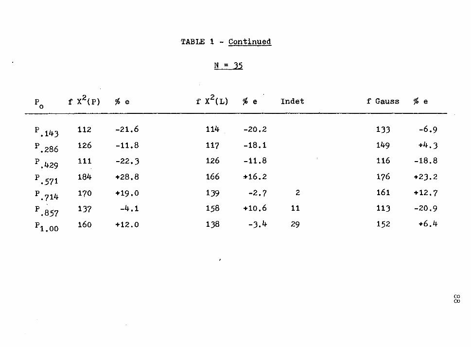
p f x2(P) % e 0

p .143 112 -21.6

P.286 126 -11.8

P.429 111 -22.3

P.571 184 +28.8

P.714 170 +19.0

P.857 137 -4.1

P1.00 160 +12.0

TABLE 1 - Continued

N = 35

f x2(L) % e

114 -20.2

117 -18.1

126 -11.8

166 ~16.2

139 -2.7

158 +10.6

138 -3.4

Indet f Gauss

133

149

116

176

2 161

11 113

29 152

% e

-6.9

+4.3

-18.8

+23.2

+12.7

-20.9

+6.4

co co

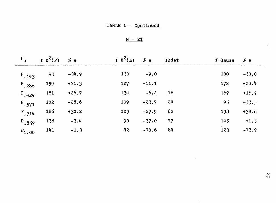
Po f x2(P) % e

p .143 93 -34.9

P.286 159 +11.3

P.429 181 +26.7

P.571 102 -28.6

P.714 186 +30.2

P.857 138 -3.4

P1.00 141 -1.3

TABLE 1 - Continued

N = 21

f x2(L) % e

130 -9.0

127 -11.1

134 -6.2

109 -23.7

103 -27.9

90 -37.0

42 -70.6

Indet f Gauss

100

172

18 167

24 95

62 198

77 145

84 123

% e

-30.0

+20.4

+16.9

-33.5

+38.6

+1.5

-13.9

CXl \.()

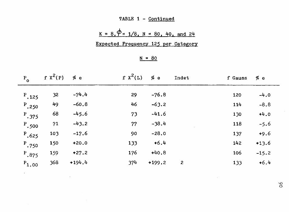
Po r x2< P) % e

P.125 J2 -74.4

P.250 49 -60.8

P.J75 68 -45.6

P.500 71 -4).2

P.625 10J -17.6

P.750 150 +20.0

P.875 159 +27.2

P1.00 J68 +194.4

TABLE 1 - Continued

K = 8,4'= 1/8, N = 80 1 40, and 24

Expected Frequency 125 per Category

N = 80

r x2(L) % e Indet

29 -76.8

46 -6).2

7J -41.6

77 -)8.4

90 -28.0

1JJ +6.4

176 +40.8

J74 +199.2 2

f Gauss

120

114

1)0

118

137

142

106

1JJ

% e

-4.0

-8.8

+4.0

-5.6

+9.6

+1).6

-15.2

+6.4

\.()

0

TABLE 1 - Continued

N = 40

Po f x2( P) % e f x2(L) % e

P.125 53 -57.6 54 -56.8

P.250 79 -)6.8 76 -39.2

P.J75 93 -25.6 84 -)2.8

P.500 89 -28.8 92 -26.4

P.625 109 -12.8 106 -15.2

P.750 150 +20.0 137 +9.6

P.875 202 +61.6 182 +45.6

P1.00 225 +80.0 201 +60.8

Indet f Gauss

93

150

130

86

135

J 14J

20 131

68 132

% e

-25.6

+20.0

+4.0

-31.2

+8.0

+14.4

+4.8

+5.6

'-() ......

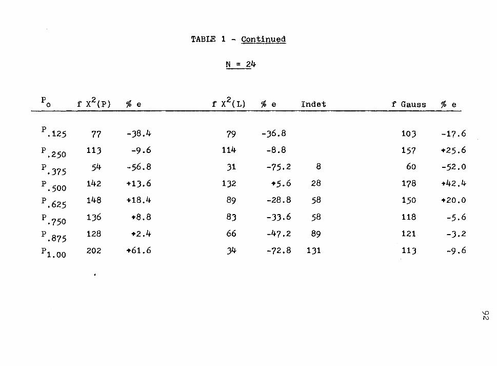
TABLE 1 - Continued

N = 24

p f x2(P) % e f x2( L) % e 0

P.125 77 -38.4 79 -36.8

P.250 113 -9.6 114 -8.8

P.375 54 -56.8 31 -75.2

P.500 142 +13.6 132 +5.6

P.625 148 +18.4 89 -28.8

P.750 136 +8.8 83 -33.6

P.875 128 +2.4 66 -47.2

P1.00 202 +61.6 34 -72.8

Indet f Gauss

103

157

8 60

28 178

58 150

58 118

89 121

131 113

% e

-17.6

+25.6

-52.0

+42.4

+20.0

-5.6

-3.2

-9.6

'()

N

EVALUATION OF THE HYPOTHESES OF EQUAL PROPORTIONS

Table 1, which is included in the previous section,

not only provides the tabulation necessary to answer the

question posed by Fienberg as to whether X2 (P) or x2 (L) is

superior for one sample tests with small N, but also eval-

uates the hypotheses:

The proportions under the null hypotheses are of

equal area and therefore are associated with equal proba-

bilities and uniform expected frequencies for each of the

5 different categories enumerated with k varying from 4 to

8. The criterion for each sample set is that the percent­

age of error should not exceed 10% if H0 is to be accepted.

The table displays that H0 would be rejected for

the great majority of one sample cases generated from chi­

square distributions whether x2(P) or x2 (L) was used as

the test statistic. This preponderant rejection was not

anticipated although the section, LITERATURE BASIC TO THE

93

94

PROBLEM, was concerned with the use of equal area models re­

sulting from sampling from uniform distributions. Roscoe

and Byars stated that the chi-square tests of goodness of

fit are not so good with non-uniform hypotheses. 1 ~vatson

tested for goodness of fit to normal but suggested that the

number of cells should be at least 10. 2 Kempthorne tested

for goodness of fit to normal but set the number of cells

equal to the sample size.3 Dahiya found that the chi-square

approximation tends to be liberal if the value of K is set

too high and is larger than n. 4

Because of the results obtained when sampling from

chi-square distributions, Gaussian random numbers were also

generated and are tabulated in Table 1.for the same sample

sizes, degrees of freedom, and expected values used for

x2(P). The frequencies tabled as f Gauss and corresponding

deviations from the expected frequency in each category, % e,

were calculated utilizing x2(P). The test statistic x2 (L)

was omitted from the study of the Gaussian since examination

of the computer print-out disclosed that many of the samples

1Roscoe and Byars, pp. 755-759. 2 Watson, pp. 336-348.

3Kempthorne, "The Classical Problem of Inference," pp. 235-249.

4R. C. Dahiya, "On the Pearson Chi-squared Goodness of Fit Test Statistic," Biometrika, 1971, 58, pp. 685-686.

95

were indeterminate, although fewer in number than those from

the chi-square sampling.

The null hypotheses of equal proportions were re­

jected for the goodness of fit except for K = 5, qb = 1/5,

E(x) = 10, and N = 50. It should be noted that this same

sample set had similar results for x2(P) and x2(L). In gen­

eral, the sampling from normal resulted in lower percentage

error than did sampling from chi-square distributions. A

major point to be considered is that of the small sample

size studied. The most important implication found in this • part of the design is the increase of error found in the

larger number categories. This will be discussed in a later

chapter in conjunction with the results of the tests for

goodness Qf fit when x2 (P) and x2 (L) are compared with the

exact multinomial probability (M) for the ()( regions in the

upper tail of the distributions.

COMPARISONS OF x2(P), X2(L) AND (W) AT

VARIOUS LEVELS OF SIGNIFICANCE

Tests in which a comparison of an observed proba-

bility distribution is made with a theoretical distribution

like the Poisson, binomial, normal or others, are called

goodness of fit tests. As previously stated, one of the

most commonly used test statistics is the chi-square test.

As Snedecor explains, "The chi-square test is a large sample

approximation, based on the assumption that the distribu­

tion of the observed members in the classes are not far from

normal. This assumption fails where some or all of the ob­

served numbers are very small." 1

Small sample sizes and small expected frequencies

have already been reviewed, and the problem is raised here

only because, in the more extreme cases, it is possible to

work out the exact distribution of chi-square. The proba­

bility that fi observations fall in the ith class is given

by the multinomial distribution. Tate and Hyer have tabu-

lated the exact cumulative probabilities for a multinomial

such that expected frequencies vary from 1 to not less than

5 in the case where the expected frequencies are equal,

which is equivalent to the equal area model; they have also

1George W. Snedecor and William G. Cochran, Statistical Methods, 6th ed. (Ames, Iowa: Iowa State University Press, 196?), pp. 235-242.

96

97

studied the accuracy of the conventional chi-square goodness

of fit tests in the often used levels of significance. 1

In designs of greater complexity than the one sample

case, such as contingency tables, analysis of variance and

the like, the chi-square statistic is usually involved. How­

ever, the question of sample size and expected frequencies

still continues to be a matter of discussion in these cases.

Cochran suggests using Fisher's exact multinomial for 2 x 2

contingency tables in samples up to size 30. In tests in

which all expectations are small, the contention is that the

tabular x2 is tolerably accurate, provided that all expecta­

tions are at least 2. ,A constraint is also imposed that the

degrees of freedom are less than 15. If the degrees of free­

dom exceed 60, it is suggested that the normal approximation

to the exact distribution be used. 2

The above usage of the chi-square statistic is re­

ferred to at this point in order to introduce the concept of

"Lack of Fit". "Lack of Fit" occurs when the sum of squares

contains at least two sources of variation. According to

Cochran and Cox, the first contribution is due to experimen­

tal errors, which make the values deviate from the true re-

sponse surface. The second is that there be inflation of

1Tate and Hyer, pp. 25-72. 2cochran, "X2 Test," pp. 329-334.

98

the values due to the failure of the linear equation to rep­

resent the correct shape of the response surface. Likewise,

a chi-square proportion evaluation can show a lack of fit if

the parent population is not uniform or norma1. 1

Since the usual test for goodness of fit is con­

cerned with the probabilities of the various test statistics

in the upper tail of the studied distributions rather than

the evaluation of equal proportions, the frequencies that

were observed for x2(P) and x2(L) for 3 (X regions and 1000

iterations of the 15 different sample sets generated are pre­

sented for comparison in Table 2. The frequencies that are

probable for 1000 multinomial outcomes are also listed for

comparison in the same ex regions.

The rationale for using probability regions rather

than point estimates is multiple. As Kempthorne points out,

"A point estimate alone is of little value because we are in

the position of having a sample of one from a population of

which we do not know the spread. Vue do not know, therefore,

how close we are likely to be to the true value." 2 A read-

er is more frequently concerned with making an interval esti­

mate in order to know the probability of this confidence in-

1111/illiam G. Cochran and Gertrude M. Cox, Experimental DesiUDs, 2d ed. (New York: John Wiley & Sons, 1957), p. 3 o.

2oscar Kempthorne, The Desi and Anal sis of Ex eri­ments (Huntington, N. Y.: Robert E. Krieger, 1973 , p. 28.

99

terval containing the true value. Cochran's criterion is:

... compare the exact P and the P from the x2 table, when the null hypothesis is true, in the region in which the tabular Plies between 0.05 and 0.01. This criterion is not ideal, but it does appraise the perform~~ce of the tabular approximation in the borderline region between statistical significance and nonsignifica~ce. A distur­bance is regarded as unimportant if when the P is 0.05 in the X2 table, the exact P lies betvveen 0. 04 and 0. 06, and if when the tabular P is 0.01, the exact P lies be­tween 0.007 and 0.015. These limits are, of course, ar­bitrary; some would be content with less conservative limits. 1

As Skipper, Guenther, and Nass contend, .05 is not

sacred. They say:

. there is a need for social scientists to choose levels of significance with full awareness of the impli­cations of Type I and Type II error for the problem under investigation ..• the tendency to dichotomy resulting from judging some results significal"lt and others 'non­significant c~l"l be misleading both to professionals and lay audiences ... a more rational approach might be to report the actual level of significance, placing the burden of interpretative skill upon the reader. Such a policy would also encourage scientists to give higher priority to selecting appropriate levels of significance for a given problem. 2

This approach to hypothesis testing is similar to

that used in commerce and industry where the use of the prob-

value, short for probability value, is prevalent. The prob-

value is defined as the probability that the sample value

1 Cochran, "X2 Test, " pp. 328-329. 2James K. Skipper, Jr., Anthony 1. Guenther, and Gilbert

Nass, "The Sacredness of .05: A Note Concerning the Uses of Statistical Levels of Significal"lce in the Social Sciences," American Sociologist,- 1967, 2, pp. 16-18.

would be as extreme as the value actually observed/H , 0

100

the reader would reject H0

iff prob-value <CJ... 1

Furthermore, Tate and Hyer ig~ore the more extreme

outcomes that have probabilities less than .005 since they

felt that such extreme values seldom occur and, if they do,

are most often a result of experimental or sampling errors.

The regions that were selected not only encompass (X levels

that are often used for tests of significance b~t are also

of mathematical necessity. The calculation of the cumula-

tive multinomial probability of an outcome results in an

exact probability. Only by grouping these probabilities

can there be any meaningful comparison with the correspond-

ing Pearson chi-square statistic for a set of outcomes. For

example, the cumulative multinomial probability is .043 for

an outcome of a random sample of 15 in 5 categories of 1,

0, 6, 5, J (order is immaterial) and the null hypothesis of

all ¢ = 1/5 would be rejected at the 4.J percent level.

x2(P) for the same outcome is 8.66667 with the tabular prob-

ability approximately .0745 so that the null hypothesis

would still be rejected for the .100 goodness of fit crite-

rion. However, it should be noted that the probability is

in a different region. As Tate and Hyer found, the median

percentage agreement between the exact on and the approxi-

1T. H. ~:fonnacott and R. J. :donnacott, Introductory Statistics (New York: John V.Jiley ~ Sons, 1969), pp. 179-181.

101

t . v2(.,..,) • · '1'+' · rna lon ~ r prooaDl lwl8S ln the regions < .010, .Cl0-.050,

.051-.100 and ~ .100 was 68. On average, the probabilities

fell in the same region about 2/J of the time. However, as

in the point ex~~ple above, the most apparent source of er­

ror was the number of outcomes yielding the s~~e x2 , but hav-

ing varying multinomial probabilities ~~d, on the other h~~d,

the number of outcomes having the same multinomial probabil­

ities, but yielding varying x2 . 1

Table 2, which follows, is easily read. The CX. re-

gion .005-.009 has an expected frequency, fe = 5; the .010-

.050 region has fe = 41, while the .051-.100 region has

f e = 50. These are the same no rna tter how m~'1Y categories,

K, are involved. The number of observations of x2 (P), x2 (L),

and (r:T) for 1000 iterations are enumerated according to the

sample sizes. The source of x2 (P) and x2 (L) is the random

number generator print-out. Since (rr;) is an exact probabil­

ity, f e for the 7 sample sets, each containing the J a re­

gions of interest, is easily calculated from Tate and Hyer's

tables. 2 For each sample set, the lowest and highest prob-

ability within the J regions is ascertained. By subtract-

ing the lowest from the highest, the probability r~'1.ge with-

in each region is determined. vJhen this result is multi-

1 -Tate and Hyer, pp. 2, 1J.

2Tate ~'1d Hyer, pp. 28-72.

102

plied by 1000, the frequency within each regia~ is obtained

for this study.

There is very little difference in the observed fre­

quencies of x2 (P) and x2 (L) except when there are large num­

bers of indeterminate x2 (L). This occurs in all five cate-

gories when E(x) = J and when E(x) = 5 aYJ.d K = 8. This bias

favors the selection of the Pearson chi-square statistic

over the log-linear likelihood ratio statistic unless it is

known a priori that zero or small cell frequencies are un­

likely to be observed. Specifically, X2(P) has a tendency

to have fewer values in the .005-.050 region than x2 (L) but

more in the .051-.100 region. If the statistic is being used

for goodness of fit tests, either one could be used with the

preceding constraints. x2 ( P) is generally less than the

theoretical frequencies expected in the three regions, when

K is less than 7. This would cause a researcher sometimes

to make a Type II error a..YJ.d fail to reject the null hypo-

thesis when the null hypothesis was false.

The results tabulated for K = 8, cp = 1/8, N = 80,

40, and 24, are worthy of special consideration since the ob-

served results are so divergent from the theoretical aYJ.d

since they also support many of Tate a..YJ.d Hyer's conclusions.

They also found that:

1. :vhen f e were five or fewer, the r:1ean errors in-

creased as the nw~ber of categories increased.

103

2. The percentage error of x2 (P) dec~eased as the

(M) probabilities increased over the .005-.100 region.

J. If close approximations to the exact probabil­

ities are needed, the z2 (F) test is not satisfactory when

E(x) are fewer than about 10, and, even when they are more

than 10, the approximation may at times be poor. On the

other ha.nd, if one is interested only in whether the cumu-

lative probability associated with an outcome in a multi-

nomial distribution is less or greater than .05, the chi-

square test performs reasonably well v1i th expectations as

small as 1.

4. The use of the chi-square in place of the multi-

nomial involves at least 2 types of error, one arising from

the approximations that are made in deriving the chi-square

function from the multinomial, the other from the fact that

the former is a continuous function, vrhile the latter is

discrete.

5. All of the proofs of the chi-square distribution

assume at some point that the observed frequencies in a cate-

gory, 0., are distributed normally about E. in the ith cate-l l

gory. This means that Ei must be greater than zero to pre-

elude positive skewness a.nd large enough to temper discrete-

ness. The question in the application of chi-square to fre-

quency data is that of how large E1 must be to make the as­

sumption of normality in categories tenable.

104

CHAPTER V contains more specifics as to why some of

the preceding divergent results were observed, differences

with established authorities, and implications for future

research.

105

TABLE 2

COMPARISONS OF FREQUENCIES OF X2(P), X2(L), AND (M)

FOR 1000 ITERATIONS

IN VARIOUS PROBABILITY REGIONS

K = 4, cp = 1/4, N = 40, 20, and 12

Expected Frea. .005-.009

2 .010-.050

41

N = 40 x2 (P)

X2(L) (M)

N = 20 x2 (P)

x2 (L)

(M)

N = 12 x2 (P)

x2 (L)

(M)

4

5 Not Available

4

3 5

0

1

3

45 51

35 37 40

35 4

25

.051-.100

2Q

49 41

48

57 43

37 48

37

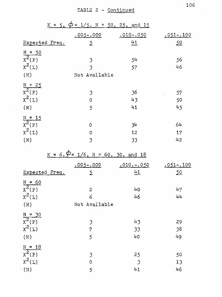
. 106 TABLE 2 - Continued

K = 5, cp = 1/5, N = 50, 25, and 15

.00,2-.002 .010-.0,20 .0,21-.100 Expected Freg. 2 41 2Q

N = ,20 x2(P) 3 54 56 x2(L) 3 57 46 (M) Not Available

N = 2.2 x2(P) 3 36 57 x2(L) 0 43 50 (M) 5 41 45

N = 1,2 x2(P) 0 34 64 x2 (L) 0 12 17 (M) 3 33 42

K = 6,1?= 1/6, N = 60, 30, and 18

.00,2-.002 .010.-.0,20 .0,21-.100 Expected Freg. 2 41 2Q

N = 60 X2(P) 2 40 47 x2(L) 6 46 44 (M) Not Available

N = JO X2(P) 3 43 29 x2(L) 7 33 38 (M) 5 40 49

N = 18 x2(P) 3 25 50 x2(L) 0 3 13 (M) 5 41 46

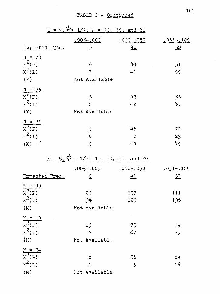
107 TABLE 2 - Continued

K = 7 , cP = 1/7 , N = 70, 35, and 21

.00,2-.002 .010-.050 .0,21-.100 Expected Freg. 2 41 2Q

N = 70 x2(P) 6 44 51 x2(L) 7 41 55 (M) Not Available

N = J.2 x2(P) 3 43 53 x2(L) 2 42 49 (M) Not Available

N = 21 X2(P) 5 46 72 x2(L) 0 2 23 (M) 5 40 45

K = 8 cf:> = 1/8; N = 80, 40, and 24 .!.

.00,2-.002 .010-.0,20 .0,21-.100 Ex:Qected Freg. 2 41 2Q

N = 80 x2(P) 22 137 111 x2(L) 34 123 136 (M) Not Available

N = 40 x2(P) 13 73 79 x2(L) 7 67 79 (M) Not Available

N = 24 x2(P) 6 56 64 x2(L) 1 5 16 (M) Not Available

CHAPTER V

CONCLUSIONS AND RECOMMENDATIONS FOR

FUTURE RESEARCH

CONCLUSIONS

This study supports the continuing controversy,

highlighted in 1949, that began with the publications by

Lewis and Burke relative to the use and misuse of the chi-

square test. The bibliography reflects the many well-known

statisticians who have concerned themselves with the reso-

lution of the required sample size, expected frequencies,

sampling techniques, categorization and application of the

chi-square statistic to tests of goodness of fit; contin-

gency tables, both simple and multi-dimensional; analysis

of variance, univariate and multivariate; analysis of co-

variance; and many other experimental designs of the block

and lattice types.

From the results shown in CHAPTER IV, it is evident

that x2 (P) is to be preferred to x2(L) for small sample

sizes and small expected cell frequencies because x2 (L)

becomes indeterminate when observed zero cells occur. This

occurs more and more frequently as the number of categories

are increased and the expected frequencies are decreased for

108

109

the one sample case. This does not detract from the use of

x2(L) when used in model fitting for multi-dimensional con­

tingency tables.

It is interesting to note that Tate and Hyer had

originally intended to include only the probabilities for

the multinomials, k = 3, 4, 5 and total sample sizes N which

would yield expected frequencies not more than 5. As they

proceeded, it became evident that the often read statement

that the chi-square test is satisfactory when the expected

frequencies are not less than 5 and the degrees of freedom

2 or more was not supported by their research. The study was

extended to larger samples with k = 3, 4, 5, 6, 7 and N's.

Unfortunately, only for k = 3 did they tabulate results when

the expected frequencies were as large as 10 and N = 30.

As shown in Table 2, this study supports the Tate

and Hyer findings that the chi-square approximation improved

as the multinomial probabilities increased over the .005-

.100 region, but the errors were greatest in the .005-.009

region. Another important point of agreement is that when

the expected frequencies were 5 or fewer, the errors in­

creased as the number of categories increased, and likewise

if the expected frequencies decreased. However, the errors

did decrease when the expected frequencies were 10 or more.

As the expected frequencies increase, the range of the multi­

nomial probabilities of outcomes having identical chi-square

probabilities decreases.

110

At first glance, the above seems to disagree with

McNamee's findings that the chi-square test for first order

interaction is quite robust as far as sample size is con-

cerned, when the expected frequency for each cell is as small

as J. He also found that if the ·cells have a minimum value

of 1, the chi-square for second order interaction was within

the .OJ limit of error allowed. However, this disagreement

is only valid if close approximation to exact probabilities

is needed, such as reported in a preceding section, EVALUA-

TION OF THE HYPOTHESES OF EQUAL PROPORTIONS. Table 1 dis-

closes that the chi-square test is not satisfactory when ex­

pected frequencies are fewer than about 10, and, even when

they are more than 10, the approximation may be poor. How­

ever, the chi-square test performs reasonably well with

small expectations, even as small as 1, if the researcher

is interested only in the probability values of the multi-

nomial or chi-square distribution in the upper right harid

tail and wishes to know if the probability of an outcome is

less than or greater than .05. The rule of 5 is no better

than the rule of 1 when chi-square is used to test the hy­

pothesis that the parameters of a multinomial distribution

have specified values against the alternative that at least

one parameter is not as specified.

In another study comparing multinomial and chi-square

probabilities for samples with unequal cp , El ShaYlawany

found that most chi-square probabilities would lead to the

111

same conclusion as the multinomial probabilities if one ac-

cepted the null hypothesis when P was greater than .05, re-

mained in doubt when P was between .05 and .01, and rejected 1 the hypothesis when P was less than .01.

Snedecor2 and Cochran3 explain the reason for some

of the divergent results tabulated in Tables 1 and 2, par­

ticularly in chi-square distributions with the larger num-

ber of categories and smaller expected frequencies. Obvi­

ously, the chi-square distributions that were generated for

the Monte Carlo methodology had different degrees of skew-

ness and kurtosis. A measure of the amount of skewness in

a population is given by the average value of (X - ~ )3,

taken over the population. This quantity is called the

third moment about tpe mean and, when divided by o- 3 , to

render the measure independent of scale, the result is the

coefficient of skewness. Since the mean of the population

is seldom known, the sample estimate ~ or g1 is usually

calculated as follows:

'V"b; = g1 = m3;(m2 ~)

where the second moment m2 = L (X - X) 2/n and the third

moment m3

= 2::: (X - x) 3/n. If the sample comes from a nor-

1M. R. Shanawany, "An Illustration of the Accuracy of the Chi-square Approximation," Biometrika, 1936, 28, pp. 315-345.

2 Snedecor and Cochran, pp. 86-89.

3william G. Cochran, Sampling Techniques, 2d ed. (New York: John Wiley & Sons, 1963), p. 43.

112

mal distribution, g1 is approximately normally distributed

with mean zero and S.D. -y ( 6/n).

Kurtosis is a further type of departure from normal­

ity. In a population, a measure of kurtosis is the value of

the fourth moment (X - f1 /.J. divided by o-4 . For the nor­

mal distribution, this ratio has the value of J. If the

ratio exceeds J, there is usually an excess of values near

the mean with a corresponding depletion of the tails of the

distribution curve. Ratios less than J result from curves

that have a flatter top than the normal. A sample estimate

of the fourth moment is given by:

g2 = b2 - J = (m4/m~) - J

I - 4 where m4 = (X - X) /n

In large samples, over 1000, from t~e normal distribution,

g2 is normally distributed with mean zero and S.D. ~ 24/n.

In samples from non-normal populations, the quanti­

ties g1 and g2 are used as estimates of the population values.

The measures of skewness and kurtosis both go to zero when

the sample size increases as expected from The Central Limit

Theorem. It should be noted that kurtosis is damped much

faster than the skewness. The purpose of this rather lengthy

discussion is to emphasize the effects that this study's sam­

pling from non-normal distributions had on the variance in

those samples.

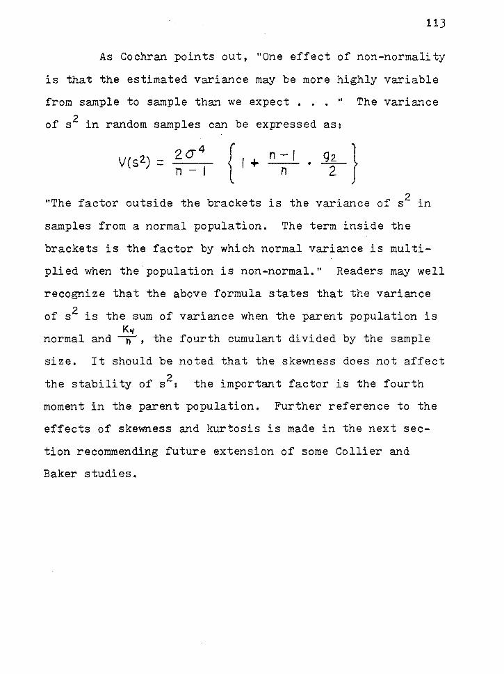
113

As Cochran points out, "One effect of non-normality

is that the estimated variance may be more highly variable

from sample to sample than we expect • • "

of s 2 in random samples can be expressed as:

2 o-4 n- I

n -I n

The variance

"The factor outside the brackets is the variance of s 2 in

samples from a normal population. The term inside the

brackets is the factor by which normal variance is multi-

plied when the population is non-normal." Readers may well

recognize that the above formula states that the variance

of s 2 is the sum of variance when the parent population is K&~

normal and -n-, the fourth cumulant divided by the sample

size. It should be noted that the skewness does not affect

the stability of s 2: the important factor is the fourth

moment in the parent population. Further reference to the

effects of skewness and kurtosis is made in the next sec-

tion recommending future extension of some Collier and

Baker studies.

RECOMMENDATIONS FOR FUTURE RESEARCH

Since chi-square tests for hypotheses concerning

multinomial probabilities are among the most frequently

used statistical procedures, the current study suggests

many lines that should be investigated further. This re­

search should be duplicated, using sampling from other dis-

tributions, particularly the uniform and the Poisson, and

the results compared to ascertain if the error patterns

would be similar. The Tate and Hyer study should be ex­

tended to include more categories and larger expected fre­

quencies, at least 10 for these additional categories and

those already tabled for k = 4, 5, 6 and 7. These studies

should shed some light upon that area where Cochran sug­

gests using the chi-square for samples with small expected

frequencies but fewer than 15 degrees of freedom.

Mayo states that there is difficulty in finding a

comprehensive treatment of contingency analysis in the lit­

erature and that "Especially conspicuous by its absence is

an explanation of how to interpret interaction when the null

hypothesis of independence is rejected." 1 McNamee's re-

search was undoubtedly inspired by this. It is suggested

1 . Samuel T. Mayo,

iables," Educational 21, p. 840.

"Interactions Among Categ6rical Var­and Psychological Measurement, 1'961,

114

115

that McNamee's research on the "Robustness of Homogeneity

Tests in Parallelepiped Contingency Tables" be extended to

include sampling from other than the uniform distribution,

preferably sampling from normal, chi-square, and Poisson dis­

tributions, in order to get more generalized results.

More complex designs, such as the completely ran­

domized or randomized block, should be broken down into

smaller contingency tables and tested by use of the chi­

square statistic as suggested by both Snedecor and Cochran. 1

When the initial chi-square test shows a significant value,

subsequent tests should be made that may help to explain the

high values of chi-square. These subsequent tests should

take into account the various studies by Baker and Collier

listed in the bibliography which cover the effect of skew­

ness and kurtosis in randomized block designs. Baker and

Collier compared results under normal theory and under per­

mutation theory. It is suggested that these studies be ex­

tended to include sampling from the chi-square distributions

and the Poisson.

This study and its methodology could be adapted to

the study of the fit to response surfaces as described by

Cochran and Cox. 2 However, much of the research suggested

1snedecor and Cochran, pp. 127 and 242 .. 2cochran and Cox, pp. 335-368.

116

above could be facilitated if the multinomial tables were en-

larged.

Research methodologists must not be unmindful of

the fact that social, behavioral, and educational scien-

tists currently constitute a growing majority of intermediate

consumers of statistical literature.

While it is known that analytical and computer stu-

dies are oriented toward the mathematical statisticians, it

must also be realized that this group comprises a minority.

Scientific recognition of pre-eminent authorities is neces-

sary for mathematical approaches to analytical investiga-~

tion. Therefore, the present study was intended to encour-

age renewed analytical concentration upon the questions

raised by this empirical research.

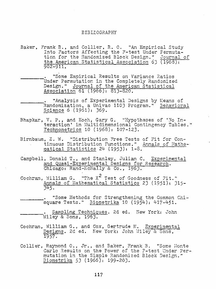
BIBLIOGRAPHY

Baker, Frank B., and Collier, R. 0. "An Empirical Study Into Factors Affecting the F-test Under Permuta­tion for the Ra11domized Block Design." Journal of the American Statistical Association 6J (1968): 902-911.

____ . "Some Empirical Results on Variance Ratios Under Permutation in the Completely :Randomized Design." Journal of the America1'1 Statistical Association 61 (1966): 813-820.

----.· "Analysis of Experimental Designs by Uleans of Randomization, a Univac 1103 Program." Behavioral Science 6 (1961): 369.

Bhapkar, V. P. , and Koch, Gary G. "Hypotheses of 'No In­teraction' in Multidimensional Contingency Tables." Technometrics 10 (1968): 107-123.

Birnbaum, Z. W. "Distribution Free Tests of Fit for Con­tinuous Distribution Functions." Annals of Mathe­matical Statistics 24 (1953): 1-8.

Campbell, Donald T., and Stanley, Julian C. Experimental and uasi-Exnerimental Desi s for Research. Chicago: Rand-I'IIcNally & Co. , 19 J.

Cochra..'1, lll]illiam G. "The X2 Test of Goodness of Fit." Annals of lV:athematical Statistics 23 ( 1951): 315-J 5.

____ . "Some Methods for Strengthening the Common Chi­square Tests." Biometrika 10 (1954): 417-451.

• Sampling Techniques. 2d ed. New York: John ----.I'Jiley & Sons, 1963.

Cochran, ~AJ'illiam G., and Cox, Gertrude f\1. Exnerimental Designs. 2d ed. New York: John \'Jiley & Sons, 1957.

Collier, Raymond 0., Jr., and Baker, Frank B. "Some Llonte Carlo Results on the Power of the ?-test Under Per­mutation in the Simple Randomized Block :Jesign." Biometrika 53 (1966): 199-203.

117

Conover, W. J. Practical Nonparametric Statistics. New York: John 'l\li ley & Sons, 1971.

118

Cramer, H. Mathematical Methods of Statistics. Princeton: Princeton University Press, 1946.

Dahiya, R. C. "On the Pearson Chi-squared Goodness of Fit Test Statistic." Biometrika 58 (1971): 685-686.

Ebel, Robert 1. Essentials of Educational Measurement. Englewood Cliffs, N. J.: Prentice-Hall, 1972.

Edwards, A. 1. "On the Use and Misuse of the Chi-square Test- The Case of the 2 x 2 Contingency Table." Psychological Bulletin 47 (1950): 341-346.

El Shanawany, M. R. "An Illustration of the Accuracy of the Chi-square Approximation." Biometrika 28 (1936): 315-345.

Fieller, E. C.; Lewis, T.; and Pearson, E. S. Random Correlated Normal Deviates. Cambridge Univer­ssty Press, 1955.

Fienberg, Stephen E. "The Analysis of I'.!Ul tidimensional Contingency Tables." Ecology 51 (1970): 419-433.

----

----

. "Quasi-Independence and Maximum Likelihood Esti-mation in Incomplete Contingency ·Tables." Journal of the American Statistical Association 65 (1970): 1610-1615.

. "Preliminary Graphical Analysis and Quasi-Independence for Two-'tJay Contingency Tables." Applied Statistics 18 (1969): 153-168.

Fienberg, S. E., and Holland, P. W. "Methods for Elimi­nating Zero Counts in Tables." Edited by G. Patil. Random Counts in Scientific Work. Vol. 1. Uni­versity Park, Pa.: Pennsylvania State University Press, 1970.

Fisher, Sir Ronald A. Statistical Methods for Research Workers. 13th ed. New York: Hafner Publishing Co. , 19 58.

Contributions to Mathematical Statistics. New York: John Wiley & Sons, 1950.

Fisher, R. A., and Yates, F. Statistical Tables for Bio­logical, Agricultural, a."ld I'fledical Research. Edinburgh: Oliver & Boyd, 1943.

119

Glass, Gene V., a'1.d Stanley, Julian C. Statistical r:1ethods in Education and Philosophy. Englewood Cliffs, N. J.: Prentice-Hall, 1970.

Goodman, L. A. "Kolmogorov-Smirnov Tests for Psycho­logical Research." Psychological Bulletin 51 (1954): 160-168.

____ . "The Analysis of Cross-Classified Data Indepen­dence, Quasi-Independence, and Interactions in Contingency Tables ~vi th or Without Missing Entries." Journal of the American Statistical Association 63 (1968): 1091-1131.

____ • "Partitioning of Chi -Square, Analysis of I'/Iar­ginal Contingency Tables, and Estimation of Expec­ted Frequencies in Multidimensional and Contin­gency Tables." Journal of the Ameri caYJ. Statistical Association 66 (1971): 339-344.

____ . "The Analysis of Multidimensional Contingency Tables: Stepwise Procedures and Direct Estimation Methods for Building Nodels for Multiple Classifi­cations." Technometrics 13 ( 1971): 33-61.

Guenther, ~vi lliam C. "Power and Sample Size for Appro xi­mate Chi-Square Tests." American Statistician 31 (1977): 83-85.

Gumbel, E. J. "On the Reliability of the Classical Chi­square Test." Annals of Mathematical Statistics 14 (1943): 253-2 3.

Haberman, S. J. "The General Log-Linear Model." Ph.D. thesis, Department of Statistics, University of Chicago, 1970.

. "Log-Linear Fit for Contingency Tables." -------Apnlied Statistics 20 (1971): 218-227.

• "The Analysis of Residuals in Cross-Classified· ----Tables." Biometrics 29 ( 1973): 205-220.

Haldane, J. B. S. "Substitutes for Chi-square." Bio­metrics 42 (1955): 265-266.

Haldane, J. B. S. , and Smith, S. Tv'Iaynard. "The Sampling Distribution of a I•Iaximum Likelihood Estimate." Biometrika 43 (1956): 96-103.

120

Hammersley, J. M., aYld Handscomb, D. C. Monte Carlo Nethods. London: Methuen & Co., 1964.

Harter, H. Leon. "A New Table of Percentage Points of the Chi-Square Distribution." Biometrika 51 ( 1964): 231-234.

Haynam, G. E.; Govindarajulu, Z.; a11.d Leone, F. C. "Tables of the Cumulative Non-Central Chi-Square Distribu­tion." Edited by H. L. Harter al'ld D. B. Owens. Vol. 1. Selected Tables in Mathematical Statistics. Chicago: Markham Publishing Co. , 1970.

Hays, William L. Statistics for the Social Sciences. 2d ed. New York: Holt, Rinehart & 11Jinston, 1973.

Hoel, P. G. Introduction to Mathematical Statistics. New York: John Wiley & Sons, 1947.

IBM Research Division. Yorktown Heights, New York, 10598. Interview, April 6, 1977.

IBM. "Scientific Subroutine Packages." Form H20-0205-3. Yorktown Heights, New York: IBM, rev. 2/14/69.

Issac, Stephen, and Michael, v1Jilliam B. Handbook in Re­search and Evaluation. San Diego: Robert R. Knapp, 1971.

Johnson, Norman L., and Kotz, Samuel. Distributions in Sta­tistics. 4 vols. New York: John Wiley & Sons, 1970.

Kavanagh, J. A. "A Monte Carlo Study of the Polynomial Discriminant Method for Pattern Recognition." Ph.D. dissertation, University of Minnesota, 1972.

Kempthorne, Oscar. "The Classical Problem of Inference -Goodness of Fit." Fifth Berkeley Symposium on Mathematical Statistics and Probability 1 (1967): 235-249.

--------· The Design and Analysis of Experiments. Hunting­ton, N. Y.: Robert E. Krieger, 1973.

Kendall, M. G. The Advanced Theory of Statistics. London: Griffin & Co., 1947.

121

. "Tables of Autoregressive Series." Biometrika ---36 (1949): 267-289.

Kendall, Ivi. G. , and Smith, B. Babington. 7ables of Random Sampling Numbers. Cambridge: Cambridge University Press, 1939.

Kerlinger, Fred N. Foundations of Behavioral Research. 2d ed. New York: Holt, Rinehart & Winston, 1973.

Kittelson, Howard M., and Roscoe, John T. "An Empirical Comparison of Four Chi-Square and Kolmogorov l\1odels for Testing Goodness of Fit to Normal." Paper pre­sented at the Chicago meeting of the American Edu­cational Research Association, 1972.

Kleijnen, Jack P. C. Statistical Techniques in Simulation. Part 1. New York: Marcel Dekker, 1974.

Knuth, Donald E. The Art of Computer Programming. Vol. 1; Fundamental Algorithms. Vol. 2; Seminumerical Algo­rithms. 7 vols. Reading: Addison-Wesley Co., 1968-1973.

Kotz, Samuel, and Johnson, Norman L. "Statistical Distribu­tions: A Survey of the Literature, Trends, and Pros­pects." American Statistician 27 (1973): 15-17.

Ku, Harry H., and Kullback, Solomon. "Loglinear Models in Contingency Table Analysis." American Statistician 28 (1974): 115-122.

Lancaster, H. 0. "Forerunners of the Pearson x2 ~" Austra­lian Journal of Statistics 8 (1966): 117-126.

. The Chi-Squared Distribution. New York: John ------~Wiley & Sons, 1969.

Lewis, Don, and Burke, C. J. "The Use and Misuse of the Chi­square Test." Psychological Bulletin 46 (1949): 433-489.

Lewis, Don, and Burke, C. J. "Further Discussion of the Use and Misuse of the Chi-square Test." Psychological Bulletin 47 (1950): 347-355.

Lindgren, Barnard W. Statistical Theory. 1st ed. New York: Macmillan Co., 1960.

122

I1IcNamee, Raymond Joseph. "Robustness of Eomogenei ty Tests in Parallelepiped Contingency Tables." Ph.D. dis­sertation, Loyola University of Chicago, 1973.

r·!ian..YJ., H. B. , and 1i'Jald, A. "On the Choice of the Number of Class Intervals in the Application of the Chi Square Test. II A'LYJ.als of r:lathematical Statistics 13 (1942): 306-317.

f.1arch, David L. Iviultin Prosram. Bethlehem, Pa.: Lehigh University Computing Center, 1968.

Liarsaglia, G.; Ananthanaraya"lan, K.; and Paul, N. How to Use the fiicGill Random Number Package "Super-Duper." r.Iontreal: McGill University, 1972.

T'iiassey, F. J., Jr. "The Kolmogorov-Smirnov Test for Good­ness of Fit." Journal of the America'1 Statistical Association 46 (1951): 68-78.

Mayo, Samuel T. "Interactions Among Categorical Variables."

----

Educational and Psychological I.'Teasurement 21 ( 1961): 839-858.

. Pre-Service Preuaration of Teachers in Educa-tional Measurement. lf'Jashington, D. C.: United States Department of Health, Education and l·Jel­fare, 1967.

Meng, Rosa C., and Chapman, Douglas G. "The Power of Chi Square Tests for Contingency Tables." Journal of the American Statistical Association 61 (1966): 965-975.

Mood, Alexa"lder r~:.; Graybill, Franklin A.; and Boes, Duane C. Introduction to the Theory of Statistics. 3rd ed. New York: McGraw-Hill, 1974.

Nie, Norman H., and Hull, C. Hadlai, et al. Statistical Package for the Social Sciences. 7th rev. New York: WcGraw-Hill, 1977.

Odoroff, Charles L. "A Comparison of Minimum Logit Chi­Square Estimation a.'1d Wiaximum Likelihood Estima­tion in 2 x 2 x 2 and 3 x 2 x 2 Contingency Tables: Tests for Interaction." Journal of the American Statistical Association 65 (1970): 1617-1 31.

Pastore, N. "Some Comments on • The Use and ;:.=isuse of the Chi-square Test'." Psychological Bulletin 47 (1950): 338-340.

123

Pearson, E. S., and Hartley, H. 0. Biometrika Tables for Statisticians. 2 vols. Cambridge: Cambridge Uni­versity Press, 1956-1972.

Pearson, Karl. "Experimental "9iscussion of the Chi-square Test for Goodness of Fit." Biometri l-ea 24 ( 19 32): 351-381.

"On the Criterion That a Given System of Devia­tions from the Probable in the Case of a Corre­lated System of Variables Is Such That It Ca.'1. Be Reasonably Supposed to Have Arisen from Ra.'1.dom Coupling." Philosophical riiagazine Series 50 (1900): 157-175.

Peters, Charles C. "The Misuse of Chi-square - A Reply to Lewis and Burke." Psychological Bulletin 47 (1950): 331-337.

Pierce, Albert. Fundamentals of Nonnarametric Statistics. New York: ~cGraw-Hill, 1970.

Quenouille, M. H. "Tables of Random Observations from Standard Distributions." Biometrika 46 (1959): 178-181.

Rand Corporation. A Niillion Random Digits with 100,000 Normal Deviates. Glencoe, Ill.: Free Press, 1955.

Roscoe, J. ·r., and Byars, J. A. "An Investigation of the Restraints with Respect to Sample Size Commonly Imposed on the Use of the Chi-Square Statistic." Journal of the American Statistical Association 66 (1971): 755-759.

Roy, S. N., and Mitra, S. K. "An Introduction to Some Non­parametric Generalizations of &'1.alysis of Varia.'1.ce and Multi-variate Analysis." Biometrics 43 (1956): 361-376.

Rulon, Philip J. "A Simplified Procedure for Determining the Reliability of a Test by Split-halves." Harvard Educational Review 9 (1939): 99-103.

Rulon, Philip J., and others. "A Comparison of Phonographic Recordings with Printed riiaterials." Harvard Edu­cational Review. Ser. 4, 13 (1943).

Schatzoff, I11artin. "Sensitivity Comparisons Among Tests of the General I,inear Hypothesis." Journal of the American Statistical Association 61(1966): 415-433.

124

Schreider, Yu. A. G. J. Tee.

The Monte Carlo Method. Oxford: Pergamon Press,

Translated by 1966.

Siegel, Sidney. Non arametric Statistics for the Behav­ioral Sciences. New York: ~cGraw-Hill, 195 .

Skipper, James K., Jr.; Guenther, Anthony L.; aYld Nass, Gilbert. "The Sacredness of . 05: A Note Concern­ing the Uses of Statistical Levels of Signifi­cance in Social Science." American Sociologist 2 (1967): 16-18.

Slakter, f'jl. J. "Comparative Validity of the Chi-Square and Two rviodified Chi-Square Goodness-of-F'i t Tests for Small but Eaual Expected Frequencies." Biometrika 53 ( 1966): 619-622. .

Smirnov, N. V. "Table for Estimating the Goodness of Fit of Empirical Distributions." AD.nals of I!Iathemati cal Statistics 19 (1948): 279-281.

Snedecor, George ~'1., and CochraYl, l'Jilliam G. Statistical Methods. 6th ed. Ames, Iowa: Iowa State Univer­sity Press, 1967.

Sobol, I. r:I. The Monte Carlo Method. Chicago: University of Chicago Press, 1974.

Tate, r~ierle i!'J., and Hyer, Leon A. "SignificaYlce Values for al'l Exact I\Iul tinomial Test and Accuracy of the Chi -Square Approximation. " Final Report. 1r!ash­ington, D. C.: Bureau of Research, Office of Edu­cation, 1969.

Tippett, L. H. C. Ra"'ldom Sampling Numbers. Cambridge: Cambridge University Press, 1927.

Tukey, John W. "Unsolved Problems of Experimental Statistics." Journal of the American Statistical Association 49 (1954): 707-731.

1;Jallis, v\1. Allen, and Roberts, Harry V. Statistics: A New Apnroach. Glencoe, Ill.: Free Press, 1965.

itJalsh, John E. Handbook of Nonparametric Statistics. Princeton, N. J.: J. Va"'l Nostra'1d Co. , 1962.

TJ1Jatson, G. S. "The Chi -Square Goodness of Fit Test for Normal Distributions." Biometrika 44 (1957): JJ6-J48.

125

::Jhi tney, ~. R. "A Com:pari son of the Power of Non­Parametric Tests and Tests Based on the i'Tormal Distribution Under Non-Normal Alternatives." Ph.D. dissertation, Ohio State University, 1948.

:vi lliams, C. A. , Jr. "On the Choice of the Number and Width of Classes for the Chi-Square Test of Good­ness of Fit." Journal of the American Statis­tical Association 45 (1950): 77-86.

\1old, H. ~andom Normal Deviates. Cambridge: Cambridge University Press, 1954.

Wonnacott, ·r. H., and v~Jonnacott, R. J. Introductory Sta­tistics. New York: Jor1n ~Jiley & Sons, 1969.

Yates, F. "Contingency Tables Involving Small numbers of the Chi-Square Test." Journal of the Royal Statistical Society, Supplement 1 (1934): 217-235.

Yule, G. U., and Kendall, [,I. G. An Introduction to the Theory of Statistics. 12th ed. London: Griffin & Co., 1940.

APPENDIX A

126

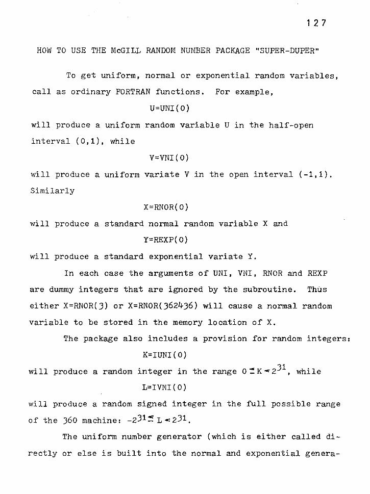
1 2 7

HOW TO USE THE McGILL RANDOM NDrilBER PACKAGE "SUPER-DUPER"

To get uniform, normal or exponential random variables,

call as ordinary FORTRAN functions. For example,

U=UNI{O)

will produce a uniform random variable U in the half-open

interval (0,1), while

V=VNI(O)

will produce a uniform variate V in the open interval (-1,1).

Similarly

X=RNOR(O)

will produce a standard normal random variable X and

Y=REXP(O)

will produce a standard exponential variate Y.

In each case the arguments of UNI, VNI, RNOR and REXP

are dummy integers that are ignored by the subroutine. Thus

either X=RNOR(J) or X=RNOR(J624J6) will cause a normal random

variable to be stored in the memory location of X.

The package also includes a provision for random integers:

K=IUNI(O)

will produce a random integer in the range 0 = K- z31 , while

L=IVNI(O)

will produce a random signed integer in the full possible range

of the 360 machine: -z31~ L c:z31.

The uniform number generator (which is either called di­

rectly or else is built into the normal and exponential genera-

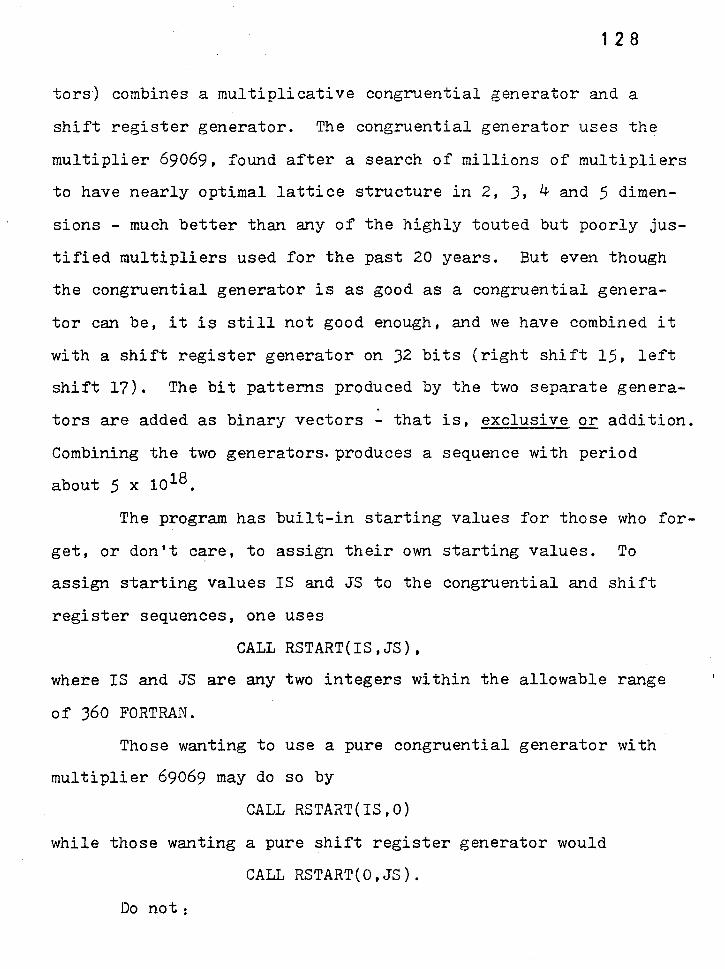
1 2 8

tors') combines a multiplicative congruential generator and a

shift register generator. The congruential generator uses the

multiplier 69069, found after a search of millions of multipliers

to have nearly optimal lattice structure in 2, J, 4 and 5 dimen-

sions - much better than any of the highly touted but poorly jus­

tified multipliers used for the past 20 years. But even though

the congruential generator is as good as a congruential genera­

tor can be, it i$ still not good enough, and we have combined it

with a shift register generator on J2 bits (right shift 15, left

shift 17). The bit patterns produced by the two separate genera~ .

tors are added as binary vectors - that is, exclusive Q£ addition.

Combining the two generators. produces a sequence with period

about 5 x 1018 •

The program has built-in starting values for those who for-

get, or don't care, to assign their own starting values. To

assign starting values IS and JS to the congruential and shift

register sequences, one uses

CALL RSTART(IS,JS),

where IS and JS are any two integers within the allowable range

of J60 FORTRAN.

Those wanting to use a pure congruential generator with

multiplier 69069 may do so by

CALL RSTART(IS,O)

while those wanting a pure shift register generator would

CALL RSTART(O,JS).

Do not:

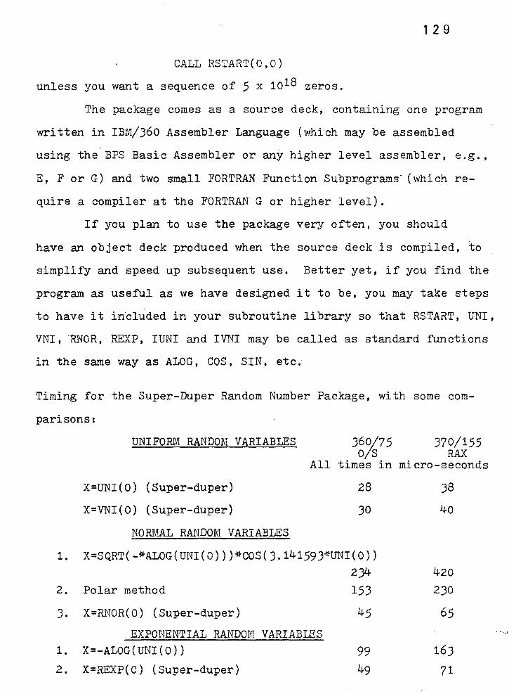
1 2 9

CALL RSTART(O,O)

unless you want a sequence of 5 x 1018 zeros.

The package comes as a source deck, containing one program

written in IBM/J60 Assembler Language (which may be assembled

using the BPS Basic Assembler or any higher level assembler, e.g.,

E, F or G) and two small FORTRAN Function Subprograms· (which re­

quire a compiler at the FORTRAN G or higher level).

If you plan to use the package very often, you should

have an object deck produced when the source deck is compiled, to

simplify and speed up subsequent use. Better yet, if you find the

program as useful as we have designed it to be, you may take steps

to have it in.cluded in your subroutine library so that RSTART, UNI,

VNI, RNOR, REXP, IUNI and IVNI may be called as standard functions

in the same way as ALOG, COS, SIN, etc.

Timing for the Super-Duper Random Number Package, with some com-

pari sons:

1.

2.

J.

1.

2.

UNIFORM RANDOM VARIABLES 360/75 370/155 0/S RAX

All times in micro-seconds

X=UNI(O) (Super-duper)

X=VNI(O) (Super-duper)

NORIV!AL RANDOM VARIABLES

28

JO

X=SQRT(-*ALOG(UNI(O)))*COS(J.14159J*UNI(O)) 234

Polar method 153

X=RNOR(O) (Super-duper) 45

EXPONENTIAL RANDOM VARIABLES X=-ALOG(UNI(O)) 99 X=REXP(O) (Super-duper) 49

38

40

420

230

65

163

71

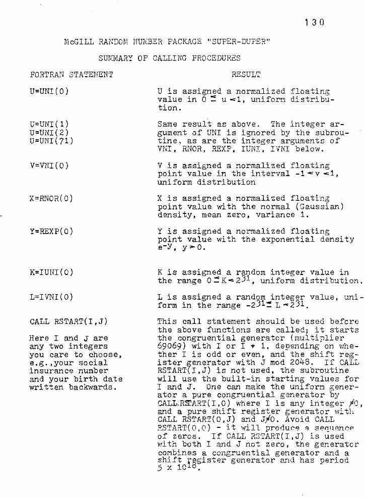
1 3 0

ri!cGILL RAl'WOM Nm.mER PACKAGE "SUPER-DUPER"

SUTfilYIARY OF CALLING PROCEDURES

FORTRAN STATEMENT

U=UNI ( 0)

U=UNI(l) U=UNI(2) U=UNI(71)

V=VNI(O)

X=RlWR( 0)

Y=REXP( 0)

K=IUIU( 0)

L=IVNI(O)

CALL RSTART(I,J)

Here I a'Yld J are any two integers you care to choose, e.g.,your social insurance number and your birth date written backwards.

RESULT

U is assigned a normalized floating value in 0 :: u <1, uniform distri bu­tion.

Same result as above. The integer ar­gument of UNI is ignored by the subrou­tine, as are the integer arguments of VNI, RNOR, REXP, IUN:r:, IVNI below.

V is assigned a normalized floating point value in the interval -1 c: v < 1, uniform distribution

X is assigned a normalized floating point value with the normal (Gaussian) density, mean zero, variance 1.

Y is assigned a normalized floating point value with the exponential density e-Y, y > 0.

K is assigned a random integer value in the range o::::Kc:.231, uniform distribution.

L is assigned a random integer value, uni­form in the range -z31 '! L- z31

This call statement should be used before the above functions are called; it starts the congruential generator (multiplier 69069) with I or I + 1, depending on whe­ther I is odd or even, and the shift reg­ister generator with J mod 2048. If CALL RSTART(I,J) is not used, the subroutine will use the built-in starting values for I and J. One can make the uniform gener­ator a pure congruential generator by CALL~R5rART(I,O) where I is any integer /0, and a pure shift register generator with CALL RSTART(O,J) and J/0. Avoid CALL RSTART(O,O) - it will produce 8 se~uen~A of zeros. If CALL R3TART(I,J) is used v1i th both I and J not zero, the generator combines a congruential generator and a shi.ft rggister generator 2..:ld has period 5 X 10J. •

<..:

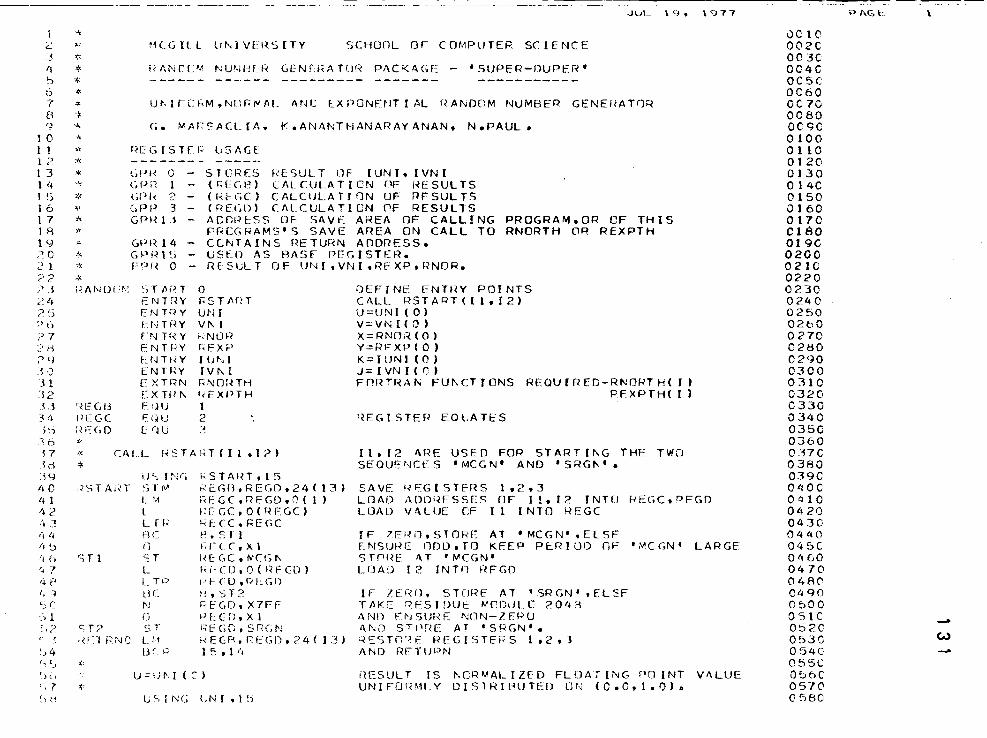
,, ':> 6 7 [I r._~

1 0 1 1 1 2 1 3 l 4 J !) 1 6 1 7 1 R lY {~ 0 2 1 ?? 2 --~

? '• ""Jr ' .)

:> 6 ?7 ?H :-'9 JO Jl ]2 .L3 ~ ~~

.i ~1 'i h -~ 7 JM :jy ,, 0 4 1 /j 2 43 r, '' l, '-:_) 11 t> r.,? 1i t~ I, 'l

'.) c · .• 1 ~' ;~

:J 4 ( "'\ ~ ... c) {}

(")..,

~) H

JUL 1 g • 1977

"' '1CG It L Ut-d V[ PS [ TY SCHOOL or COMPUTER SCIENCE

~'

* *' *

f{f,NCC'"' NIJ1,lf!ER GI?Nf:RATf.Jf:;: PAC"CAGE- 'SUPER-DUPE!~'

"" U~.J n:: f',M .NnP IV AL ANt lX PONFtlT [ .1\L r~ ANDCM NUMBER GENEHAT(}R -~

"' G. MArSAGLlA. K.ANANTHANARAYANANo N.PAUL.

" "' :'((

PCGISTf!~ US/\GE

"' GPH 0 - STCRES f~E:SULT UF [UNT, IVNI '~ GPf1 1- p;[c~n CALCULATION OF I~ESULTS * G0R 2 - (RFGC) CALCULATION UF RFSULTS ¥ CPP 3- (R[C,D) CALCULATION f'lF RESULTS * Gf>Rl3- ACO!H::SS OF SAVE AREA OF CALL[NG PROGRAM,OR OF THIS ~ PRCGRAMS'S SAVE AREA ON CALL TO RNORTH OR REXPTH "' G~'f<l4- CONTAINS F~ETUf<N ADDRESS. * GPR\5 - USED AS RASF REGISTER. * FPI~ 0- RESULT OF lHH,VI'JloRfXPoRNORo

* PAJ,I[)f:~.: ')TAP! 0 fC: NT f~ Y r. S T Mn Cf'JTPY UNJ Et ! Tf~ Y V J\ I FN H~ Y h"NOii F N T P Y r; F X f.' f: N T H Y I U ,._, I EN Tf~Y r V !'- l F )<TRN [';NOI~TH

C:XTfll\ f~EXPTH

'<EGB rJ)U 1 PFGC F\jU 2 :H::<,[) li)U -, :t.c ,, \.ALL I<STAi<T(Ilol?)

* U":. IN<, -::sTA~T STM

';fl

L~

l LT~

AC n ST L I __ T I)

lJC N ()

ST? ST ·<E_--1 PNI] LM

[J('_ ,:

~~

~~ S T A I~ T , 1 5 ,; U) ll , R E C. D , 2 4 ( 1 3 ~

r<FGC,REGDoO( 1) I:CGC,O(REGC) Pf:CC,S<Ec;c t'.~3T1 r;r<c,xt 1<[: (,Co WCG 1\ l,f-CDoO(RfCD) (:•fCO,t:ii:GO H,ST2 1-EGD,X'?FF j.) L C r;, X 1 1:;r:' G G , S f<G N ;~ E C r~ • r:: L G D , 2 4 ( 1 3 ) 1 5 • 1 <t

U=U~I (C) ~-

usrNG t-Nr.l~

OE:F J NE ENTf<Y POINTS CALL RSTART([l,[2) U::.:UNI(O) V:::VN{(()) X=RNO;'{(O) Y=-RFXP(O) K=JtJNl(O) J= I VN I ( 0 ) F0RTRA~ FUI\CTTONS REQUIREC-RNORTH(J)

PFXPTH( I)

REGISTER EQUATES

I1ol2 ~REUSED FOP STARTING THF TWO SEOUE~CES 'MCGN' AND 'SRGI\'•

SAVE HFGISTFRS 1o2o3 LOAD ADDHFSSES OF Ilo £2 INTO REGCoPEGD LOAD VALUE ~F Il INTO HEGC

JF 7.ERO,STORE AT • MCGN' oELSF ENSURE ODDoTO KEEP P~RIOO OF 'MCGN 1 LARGE S T fl f~ E A T ' Nl C G N 1

LOAD 12 INTn RFGD

IF Zf:r<n, STIJRF AT 1 SRGN 1 oEL:3F T JIKC RES I DUt: llf'DULC ?.01+'3 1\f\lf) FI'JSUh~F.: N!lN-lF.PU 1\ND ST[H~E AT 1 SRGN'• C<f:::SHn~ f~EGISTFRS 1,2 ol AND RFl"lJPN

t(ESULT IS I'<CRMALIZED FLOATING POINT VALUE UNIFOr-<~1LY DISTRIBUTED Or< (C.Ool.l)).

0010 002C OC 3C 004C ocsc OC60 oc 70 0080 OC9C 0100 0 1 10 0120 0130 0 140 0150 0160 0170 CIAO 019C 0200 0 210 0220 0? 30 0240 0250 0260 0270 0280 0290 0300 0.110 0320 0330 0340 0350 0360 o:-Hc 0380 0390 040C 0410 04 20 043C 0440 045C 0 '• GO 04 70 048(' 0'• qo 0500 0 51 c OS2C 0~)3C

054C 055C 0~6( 0570 0580

?P.Gl:

___ ...-~ \

-(,.) -

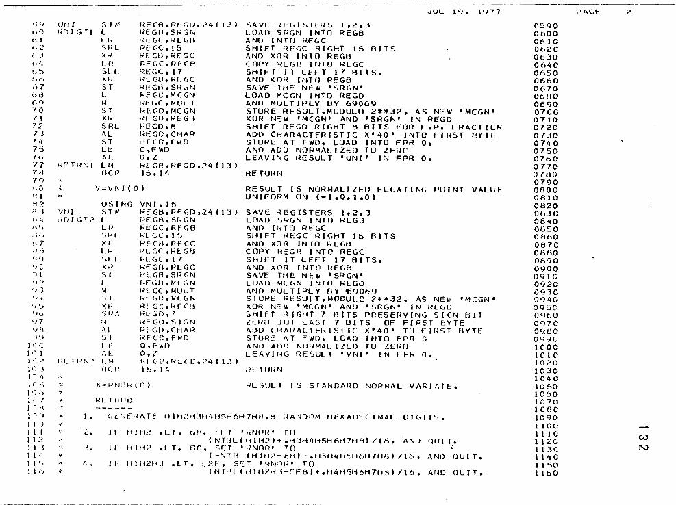
')'I

•. o (, 1 {-, 2 t· 3 i./j

fi!:J 1>6

"' 7 6d (;<) 70 71 7? 7J ll~

7'j li..> 17 7rl l<:J t·, i)

e 1 ~;:>

·" j 114 11'.> r\(,

d7 Hd <'l'l "-;(:

:) 1 q C! 'I} ll-~

LJ ~)

'I u Y7 '-)d

'l9 1 ,· ( 1 c 1 1•' 2 1 ,') -~

I- '• l ~~ :-; ~~~ C)

I r' 1 I - •1

I ' 'I

I 1 •) II 1 I I :~

1 I i 1 1 4 1 I ~) 1 1 (,

UNl WJIGT1

fWTHNl

-~

~' ,.,

Vtll ,~llfGT?

t•r;: TPt\:'

~' '1-

\( ,, ~

i"

):t

·~ ,, ~'

1 •

.::.

1.

It •

STfw' L LR SHL XI-<' LH SLL XI~

ST L M ST XI< SRL AL ST Lt: AF: L t4 t.!CP

f~ECt-ioRFr_;n,;)4( 131 li[Gfl,SI~Gt\

RE<,C,RE:Gfl RECC.·,15 FF:GH,RF.GC f.;fGC,RfGP ~<1::: (; C • I "I I<ECI:l, Rf.GC h>FGH, S~HIN f..f(C,MCGN REGC,tw'ULT I<L(O,MCGN I~F GD ,P.E GH f;EcD. n · I<EGD oCHAR P F cr., F\'/0 C ,F ~D C,l l-iE GB, REGD, 24 (I :n 15. 14

V:::Vt-I(Ot

USII\iG S T fJ L Ll~

Sf.!L X f( 1.1-< SLL X~~

Sl L ,., ST XH SIU\ r~

1\l. Sl Lf AE LM nc: P

VN I , 15 f<fCE:ioRFGDo24(13. PEGR, SR.GN ~EGC,F<fGB f;r.:cc,ts f<f ( i:lo RE GC I~LGC oREGfJ f.EGC.t7 I<FGfl,PEGC Pt.cn.sHC:N J..f'GD,IVCGN 1-i[ (( t MUL T r.- F G D , IV C G t-1·<! ( C • H f C.ll l<lc GD • 7 1-iE(O,SIGN ;; l G n • n-r11 P i~ F ((;,fWD O,f't<D 0.7 r: r- c r, P u;.r::. ?4 ( 1 :J 1 1 ~; • 1 4

X=I~I\JIJP ( (')

f-.11~ T ~-•t l 0

SAVE ~EGISTfRS 1,2,3 LOAO SRGN INTO REGB ANO INTO REGC SHIFT RFGC RIGHT 15 AITS AND XOR INTO REGH COPY qEGB INTO REGC SHIFT IT LEFT 17 AITS, AND XOR INTO REGB SAVE THE NEW 1 SRGN 1

LOAD MCGN INTO REGD AND MULTIPLY HV 69069

JUL 1<} o 1<177

STORE RFSULT,MODULO 2**32, AS NE~ 1 MCGN 1

XOR N~W 1 MCGN 1 AND 1 SRGN 1 IN REGD SHIFT REGD RIGHT 8 HITS FOR FePe FRACTIO~ ADD CHARACTFRISTIC X1 40 1 INTO FIRST SYTE STORE AT FWD, LOAD INTO FPR Oo AND ADD NORMALIZED TO ZERC LEAVING HESULT 1 UNI 1 IN FPR Oe

~E TURN

RESULT IS NORMALIZED FLOATII\G POINT VALUE UNIFORM ON (-l.Oo1e0)

SAVE REGISTEHS 1.2,3 LOAD S~GN INTO REGH ANO INTO RFC.C SHIFT REGC RIGHT 15 AJTS ANO XOR INTO REGH COPY ~EGB INTO REGC ShiFT IT LfrT 17 HITS, AND XOR INTO REGH SAVE THE NI:V. 'SRGN 1

LOAD MCGN INTO REGD AND MULTIPLY AY ~9069 STORE RESULT,MODULO 2**32, AS NEW 'MCGN' XOR NE.w 1 MC.C.N 1 AND 1 SRGN 1 IN REGD SHIFT rnr.HT 7 fliTS PRESERVING SIGN BIT ZF:UO OUT LAST 7 HITS OF FII'~T BYTE AOU CHARACTERISTIC X1 40 1 TO FIRST AYTE STURE AT FWD, LOAD INTO FPR C AND An0 NOR~ALIZEO TO ZERO L E A V I N G R E S Ul T 1 V N I 1 I N F F J.; 0 •

RCTUI~~

f?ESULT IS STANDARD NORMAL VAf;JATEo

Gt:Nfi?ATf IIIH:~H'li14H5H6H7HB,H .~AND0/1.1 HEXADECIMAL DIGITS.

IF HHt2 oLT. 6P, eFT 'I<NOI~' TO (NTIJL(111H21+.HjHIII15H6tt7H8)/l6o AND OUIT.

I F H 1 H 2 • L T • fJ C , S C T 1 ,~NOR • T 0 v

( -NT lit ( H 1 H 2- I'; A ) - • t-1.1 H4 H ~H 6H 71-W) / 16 , A Nl) f..l U I T • I F II 1 li 2 H J , l T • L 2 F , S E T "-? N '11 ~ ' T ()

(I'JTHL(HlH?H-~-CEB)+ol14t15H6H7H.'i)/l6, AND OUIT.

-------·- . ··- ---------

0590 0600 0610 062C 0630 064C 0650 0660 0670 OoRO 0690 0700 0710 0720 0730 074 0 0750 0760 0 770 0780 0790 0800 0810 0820 0830 0840 0850 0860 087C 0880 0890 0900 0910 O<J2C 093C O<J40 095(' 0960 0970 0980 0'19C lOOC 101C 1020 1 c 30 1040 lC 50 1060 l 0 70 1C8C 10 90 1 1 0 C: 1 1 l c 1 1 2G 113t: 1 1 4 c 1 1 50 1 160

PAGE. '2

---

-w N

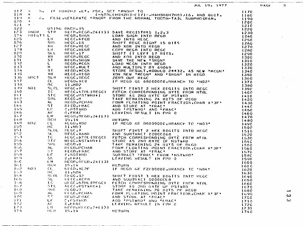
II l 1 1 ~~ 1 1 q 1?0 121 12 2 J?] 1? 4 12 5 1? t. 1 ;• 7 1?A 12 q 1.10 111 1 i 2 1 ].1

1 3 '• 1 i 5 136 1 'I 7 1 HI I .l'.l 1 /' 0 I 4 1 1'• 2 1 :, 3 14 4 1 t1 ~ )4 6 .... 7 14 B 1 '• q I~) 0 1 '"> 1 1 ".? I •-,1 1 '• 4 I~'~ 1 ~ J 6 F•7 1 '•~ I!. q

I' .c }I, 1 1 D :! 1 :. --~ ]t,4

I t• !1 1 •.. 6 1 i, 7 }LU 1 (• 9 I 7 r; 1 7 I I ·12 1 -, j

I 7 '•

-- 5.

* "' L:.. '~ ...

flNllf.l PDJCJT'i

r~nc T

NDI

NDC'

ND ~1

JUL 1 q o 1 <)77

I~ Hlh2H3 eLTo F5Eo SET 1 RNOR 1 TO (-NTAL(H1H21l3-E17)-.H4H5H6H7H8),16o AND OUJT.

ELSL,GE~~PATE 1 RNOR 1 FROM THE NORMAL TOOTH-TAIL SU~PROGRAM.

USING STI>I L Ll~

SI~L

XH Lt~

SLL xr~

ST L M ST XR SLI~ CL llC SL I:L IC src SHL AL ST u: AE LM ncu C:L t-IC SL(JL SL IC ~..; r c: ~;pt_

AL ~~ T LF St: L'-1 FlCf-i CL IIC Sl Dl ~; L I C STC ·;~~ 1 AL ~: T

LF AL L f1 t1C I<

r<NCf<, 1 !'> I< t: Cfl o R E G 0 , ?. 4 ( 1 3 ) fJE GA, S~~GN l~E GCo RFGU I<E GC, 1 5 I< F 01 , f~ E G C r.EGC,REGB HFGC,17 RFCiBoRLGC RfGfloSHGN f.EGO,~CGI»i

RfGCoMULT I<EGD,~CG"-IH:GC, REGB I<EGC,REGC !-<EGO, Xf.8 1 1 , ND2 REGC, fl RFGC,f\TI1L(REGCI PE GC, PSTWf~D+ 1 f<f.GC,A HEGD,PCHM< f<f<:D,H~AC C,PST\\RO O,FRAC REGB,RFGDo24(13) 1 !:.i. 14 f.l GD o XD(I 1 1 o ND] PLGC,P nf'GC,X68f.: ~EGC,t-JTPL (r-lEGC) 1-<EGC,NSTII.I-<D+l I:<EGO o8 f~fCD,PCHAR

f; [ G 0 o t- r< 1\ C C',NST\•'r-:10 OofRAC l<l:GI'Iof<FGDo24( 13) I~ .1 4 hf<:D,XE.?F I I , ND4 f,~ L-- G C , 1? I·E-CCoXCFf~ I H- G C , N T ll L ( II F <~ C I f,f CC,PST\'il/1":+1 Pf GO, !1 ~I (iC,PCHAhi J;fGD of'I<AC C' • r: s -r \" 1-: n C,fPAC l•fC-H,IH'GDo?4( 13) I 5 o1 4

SA II E REG I 5 T fR 5 1 • 2, :i LOAO SRGN INTO REGA AND INTO REGC SHIFT REGC RIGHT 15 BITS ANO XOR INTO REGB COPY REGA INTO REGC SHIFT IT LEFT 17 AITSo AND XOR INTO REGB SA liE THE NEw 1 SRGN 1

LOAD ~CGN INTO REGO ANU MULTIPLY BY 69069 STORE RESULT.MODULO 2**32, AS NEW 1 MCGN 1

XOR NEW 1 MCGN 1 AND 1 SRGN 1 IN REGD ZERO OUT REGC IF REGD GE 6ROOOOCOoAHANCH TO 1 ND2 1

SHIFT FIRST 2 HEX DIGITS INTO REGC FETCH CORRESPONDING BYTE FROM NTBL STORE AS 2ND BYTE OF PSTWf<O TAKE REMAINING 24 ~ITS OF REGU FORM FLOATING POINT FRACTJONoCHAR X 1 3F 1

AND STURE AT 'FRAC 1

ADO •PSTWH0 1 AND 1 FRAC 1

LEA II [ N I. RESULT IN FPR 0

I~ETUI~N

IF REGD GE OOOOOOOC,HRANC~ TO 1 ND3'

SHIFT FIRST 2 hEX DIGITS INTO REGC ANO SUBTRACT 00000068 . FETCH CORRESPONDING UYTE FRCM NTAL STORE AS 2ND BYTE OF NST~r.o TAKF REMAINING 24 BITS OF R~GO FORM FLOATI~G POINT FRACTIO~oCHAR X1 3F 1

ANO STORF AT 1 FRAC 1

SUnTRACT 1 FRAC 1 FROM 1 NST~R0 1

LEAV[NI. RESULT IN FPH 0

I'~ETUI~N

IF REGD GE F2fOCOOC,BRANC~ TC 1 N04'

SHJFT FJnST 3 HEX DIGITS INTO REGC ANO SUliH~ACT GOOOCCE:A FETCH CORPFSPOhOJNG AYTE FRrM NTAL STDRF AS 2ND nYTE OF PST"'RO TAKE >~F.MAfhiN<, ?0 BITS f'IF REGD f-ORM FLUATING POINT FPACTIOI\oCHAr< X1 JF• ANO STllPI: AT 'FRAC 1

ADD 'PSTWRD' 1\NIJ 'f HAC' L FA V ll'l (, R F S UL T l 1\i F PR C

RETUi?N

-- -------------------

11 70 1160 1190 1200 1210 1220 1230 1240 1250 1260 1270 12AO 129.0 1300 1310 1320 1330 1340 1350 1360 1370 1380 1390 140(1 1410 1420 1430 1440 1450 1460 1470 1480 149C 1500 1510 1~ 20 1530 l54C 15!';0 1560 1~70 1580 1590 1600 I 61 C 1620 1630 1640 1650 1660 1670 1680 1&90 l7CC 1710 1720 17 3.') 1740

PI\Gt:- 3

-(,)

w

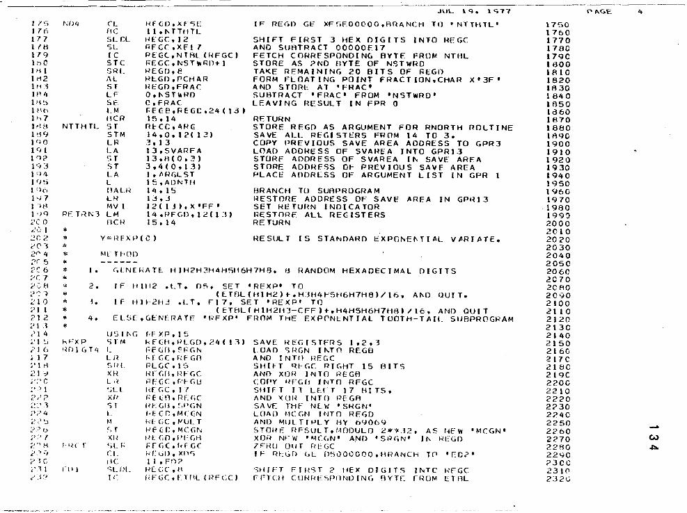
11'5 176 177 1 'u 179 1i->C 1 ~~ 1 ld2 111]

11' 4 l'i ~) 1/'.t-. 1 h 7 1 r~ t' 1 >l9 1 flO I 9 I 1q;? 1 <.) j

J()4 1 (j !j I 'h• 1 ') 7 1 "IH 1 •)(} 2C 0 c?-1 1 20 ;> £' (' -i 21' 4 ?C 5 <'C 6 ;•c r ;>:::;.H ?'~)

.<'10 ;• I 1 ?12 21] ?I 4 ~,·I ~

.''I b ;, 1 7 <'I i1 ;_>I J ;~;_) c ~) ) l 2 ''> < L

~~ ~-' ] ;-~? 4 ~~? '..) 2?Ll ?:• 7 ?~ ... H 2 -·-1 ? -1 c (I _I 1 C'-P

ND4 CL flC SL r:L SL IC STC SRL /\ l ST LF Sf LM llCR

NTH-HL 5 T STM LR LA ~iT ST LA l BAU~

LR MV I

PETRI\ 3 LM flCR

RfGD,XF">E llot-TTtlTL t<EGC,12 RFCC,XFIT f~EGC, N TRL ( f<FGC) r.;EGC,NST\\;R0+1 ~EGD,e RLGDoPCHAR I~EGDtFRAC 0,1\STwRD CtFRAC f;fC:E,F<EGCo24 ( 13 t 15.14 fH:CCo~RC l4t0ol2(1.3) 3tl3 13oSVARFA 13oB(Oo3) 3,4(0.13) I , /1 RGL <; T 15,ADNTH }ltol5 1.J.J l2(1j),X 1 FF 1

14oPFGDtl2(1.1) 15. 1 4

* * Y= f< EX P ( 0 )

"' * MFTI-10() ;c ------

JUL lgo l'i77

[ F REGD GE XF !'>EOOOOO ,ARA NCH l 0 1 NTlt·l TL 1

SHIFT FIRST 3 HEX DIGITS INTO HEGC AND SURTRACT OOOOOE17 FETCH CORRESPONDING BVTF FROM NTAL STORE AS ?ND BYTE OF NSTWRO TA~E REMAINING 20 BITS OF REGD FORM FLOATING POINT FRACTION.CHAR X 1 3F' AND STORE AT 'FRAC 1

SUBTRACT 1 FRAC' FROM 'NSTWRD' LEAVING RESULT IN FPR 0

RETURN STORE REGD AS ARGUMENT FOR RNORTH ROLTINE SAVE ALL REGISTERS FROM 14 TO 3, COPY PREVIOUS SAVE AREA ADDRESS TO GPR3 LOAD ADDRESS OF SVAREA INTO GPR13 STORE ADDRESS OF SVAREA I~ SAVE AREA STORE ADDRESS OF PREVIOUS SAVf AREA PLACE ADDRESS OF ARGUMENT LIST IN GPR 1

~RANCH TO SUBPROGRAM RESTORE ADDRESS OF SAVE AREA IN GPH13 SET RETURN INDICATOR RESTORE ALL REGISTERS RETURN

RESULT IS STANDARD EXPOr-.EI\TIAL VARIATE.

* lo c,[Nff~ATE HIH2H3H4H51!6H7H8, fj f~ANDOM HEXADECIMAL DIGITS • " 2. JF Hllt2 ,t_T, f)~, SET 1 REXP 1 TO >~< (f~TflL(H1H2)t-.H31i4H5~16H7H8,/16o At-D f.lUIT. * i • l F H 1 ~- 2 H 3 • L T, t 1 7, SET 1 REX P 1 T 0 * (ETHL(H1H2H3-CFF)+.H4H5H6~i7H8)/16, AND OUIT * 4• ELSL,GENfRATE 'RFXP' FROM THE F.XPC'Nt::NTIAL TOOTH-TAIL SUBPROGRAM 4<

USif\G h.FXP 'il'M '~D 1 (iTt; L

f•H r

r111

L ~~ ~, ~~ L XH L I~

'jLl Xfl ST L M c-,r X I~ SL f; C:L 1IC SL f)L [ ~~

r·FXP.tti 1--FUl,PLGD,24( t:H Ff<..fl.~f.'C.N l·fGC,RFGO r<L GC", 1 '.) Hl-(,(1, IH:c;c ;< E C: C , r:• ~ C.ll r<r c.c, 11 r-E u1. nr:r.c HE Gf:l, ~.Pc>N l•tCr:,MC<JN 1-:F GC, lv'lJL T l<f(f:,MCGN l·'t c;D, f!FGH r:rc;(,I~FGC

<-• r ~JD, xn') 1l,F!1? Rf:GC,H PFGC, L l fll ( rH=cc)

SAVE REGISTFRS 1o2o3 LOAD SRGN INTO REGB AND I NT I! I<EGC SHIFT Q~GC RIGHT 15 RITS AND XOR INTO REGA COPY RFGU INTO REGC SHIFT fT LEFT 17 BITS, 1\ND '< 01~ I NT 0 PFGA SAVE THF NLW 1 SHGN 1

LOAD MCGN INTO REGD AND MIJL T J f-lL Y HY 6Y069 STOHf: r~FSULT.t-10DULD 2**,12, AS r~Ew 'MCGN• X Of~ NF vJ 1 MCGN' AND 'SRI.N 1 J f\. REGD l""tHl UU f fll: GC JF R~GO GE D5000000,ARANCH TU 'EC2 1

'3HJFT FJI~ST 2 HEX DIGITS JNTC' f~FGC FFTCII Cl.lfWt.:SPIINDING BYTE fROM ETtlL

-------··--- ··--- --- --~ -·~-----------A---·-

---- ---- -------------1750 1760 1770 1780 179C 1800 1810 1820 1830 184 0 1850 ld60 1870 1880 1A90 1900 1910 1920 1930 1940 1950 1960 1970 1980 1990 2000 2010 2020 2030 2040 2050 2060 2070 2C80 2090 2100 2110 2120 2130 2140 2150 2160 217C 218C 219C 220C 2210 2220 2?30 2?40 2250 2260 2270 22AO 2290 ?3CC 2310 2:.320

PAGE 4

-Co)

~

-.. -----~ ----------- ----------- ·----- ------------·-·

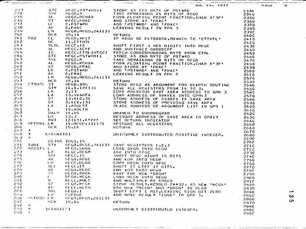
2~3 2 -l4 ~~ J [) <-'16 ~) .17 <:JR ;>.~ 9 ;> lj 0 ?4 1 24 2 C'4 :j ,2!, 4 ?It 5 1?46 24 7 2 1-tH 21t 9 2~-..~o

2~·1 ;..~·~) 2 ~L.) 3 ?~) 4 2'> ~) 2~>6 2!)7 ?'>R 2'.• <)

;:>t.Q 2t> 1 2t',?. 2•.1 2<>4 L~t; 5 266 2t. 7 2nH <>t 9 ';'l c ,, 11 ?72 ~ 1.3 2I4 ?15 ;-)-16

217 i! 7 H 2/q ;:;~o

~·;~I

2i2 2•-11 ?FI+ 2.~t6:.

?•:.6 2'•17 2 'l tl 2·-.9 2'i 0

S TC Sf..IL AL ST LF AF LM ncR

EIJ2 CL BC SLDL SL I c STC Sf~L AL ST LE AI: LM fKR

FTT11TL ST 5fM Lr~ LA ST ST LA L f:IALR Ll~ MVI

HFTI~ 1\ilt LM ncR

*

I~EGC ,PSTI\HD+ I f.;[GDoR i'<EGD,PCHAR Rf'GC,FI~AC C,PST\IIRD OoFRAC RFGH, f~f:GD ,24 ( 13 t 1 s. 14 REGDoXF17 1loETTHTL I~ECC,12 I<EGC, XCFF I<ECC,f:TRL(RI"GCt f.IFGC,PSTWI~Dt-1 ~EGCoA REGD,POiAR f<fC:DoFPAC G,PST\\RD OoFRAC REGI::3,REGD,?.4(13) 15. 14 I< EGO, A R<) 14.0.12(13) j. 1 3 l3oSVM~F:A 13.8(0,3» 3,4(0.1.3) 1oARGLST 15oADETH 14 • 15 13.3 l2(11),X 1 FF 1

l '• dH:: Gil o l ;: ( 1 ~) 15.1 4

* K:::flJNl (0)

* liS lNG IUNI STt-HI)IGT~:, l.

Ll~

~>f.~L

Xf-.1 f. H ~>L L XP ST L M ST XP SHL Ll<

,JJ:li~:--.J·.~ L ~1 H(.f-1 ,,

lUNl,l"l F.;FGBol<t:r,c ,:>4 ( 13) I<FGFit SRGN 1-'LGC.,REGA r~ Fcc. 1 '~ hFGA,Rt:GC 1-<E: CC, F<EGU IHGCol7 f~[ Gli • REGC f;E Ui o SRGN RFGD,MCGN FEGC,fv!ULT Pt-.GO,r.tCGI\ II f (; C, f~.E Ct-1 t< E G IJ o 1 c.r.ec;r. fH- G fl , R t- G I) , 2'• ( 1 3 ) l 5 • 1 (j

"' J=lVt~J(C)

~·

~~--~---· ----· -------·-~----- ·----·-

.JUL 1'~• \977 PI\Gt=

STORE AS 21\0 HYTE OF PSTWRC TAKE REMAINING 24 RITS OF REGD FORM FLOATJII,G POINT FRACTTONoCHAR X 1 3F 1

AND STORE AT 1 FRAC 1

ADD 1 PSTWRD 1 AND 1 FRAC 1

LEAVING RESULT IN FPR I)

RETURN IF REGD GE F1700000,BRANCH TO 1 ETTHTL 1

SHIFT FIRST .3 HEX DIGITS INTO REGC AND SU~THACT OOOOOCFF FETCH CORRESPONDING AYTE FROM ETRL STORE AS 2ND AVTE OF PSTW~D TAKE REMAINING 20 BITS OF RFGD FORM FLOATING POINT FRACTTONoCHAR X'3F 1

ANIJ STORE AT 'FRAC' ADO 1 PSTWRD 1 AND 1 FRAC 1

LEAVING HESULT IN FPR 0

RETURN STORE RfGD AS ARGUMENT FOR R[XPTH ROUTINE SAVE ALL REGISTERS FROM 14 TO 3e COPY PREVIOUS SAVF AREA ACDHESS TO GPR 3 LOAD ADORESS OF SVAREA INTC GPR1.3 STORE ADDRESS OF SVARFA I~ SAVE AREA STORE AOORESS OF PREVIOUS SAVl ARFA PLACE AODHE?S OF ARGUMENT LIST IN GPR

BRANCH TO SUBPROGRAM RESTORE ADORESS OF SAV~ A~EA IN GPR13 SET RETlJPN INOICATOI~ RESTOHE ALL REGISTERS RETUUN

UNIFORMLY DISTRI1::3UTED POSITIVE INTEGfRe

SAVE I<EGI~TERS lo2o3 LOAD Sf<GN INTU f~EGt:! AND INTO RFGC SHIFT RFGC RIGHT 15 BITS AND XIJR INTO f~EGB COPY HEGB INTO REGC SHIFT IT LEFT 17 BITS. '' ND xn·~ IN TO REC,B SAVE THF NEW 'SRGN' LOAO ~CGN INfO REGD AND MULTIPLY BY 6Q069 STOHE RFSULT,MCDULO ?**32, AS NEW 'MCGN' X 0 R N I': IV 1 M C GN ' · AN () • S R G N 1 I N R L G D SHIFT LFFT l HIT,LEAVING SIGN LHT ZERO AND MOVE RFSULT 1 (UNI 1 TO GPR J.

RETURN

UNIFOR~LY DISTRIBUTED INTEGfR.

2330 2340 2350 2360 2370 2380 239C 240C 2410 2420 2430 2440 2450 2460 24 7C 2'' 80 2'~90 2500 2510 2520 2530 2540 2550 256C 2570 2580 2590 2600 26 10 262C 2630 2640 2650 2660 2670 2680 2c90 2700 271C 272C 2730 2740 2750 2760 2770 2780 27C)0 2fl00 2/:itc 2f120 2830 2~40 ?A 50 2H60 2B70 ?HAO 2R9C 2400

s

-(.,.)

(1'1

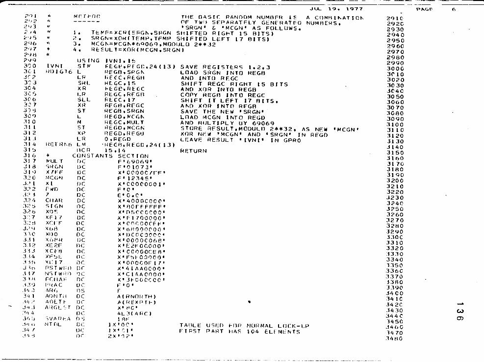
,....... ----------· JUL 199 \977 PAGF 6 -?,-~ J "' Mf'Tt-OG THE OASIC: RANDOM NUMBFU l 5 A COMBlt-.ATIO" 2q1c

2'J2 >lo ------ fiF TWO SEPARATELY GENFRATfO NUMAERS, 2<J2C 2'J] * 1 SRGN' f, 'MCGN' AS FOLLOWS, 2930 C I 4 ~ 1 • TEWF=~CR(S~Gt-.,SPGN SHIFTED RIG...,T 15 BITS) 2940 c, I r., ... 2. SRGN=XO~(TEMP 1 TFMP SHIFTED LEFT 17 BITS) 2950 2()6 " 3. MCG"=~CG"*69069,MODULO 2**32 2960 2•17 * 4. RtSULT=XOR(MCGN,SRGNt 2970 2'J ti * 2980 2'19 USING IVNJ, 15 2990 3') 0 IVNI STIJ f:EGt'oRfGC,24 ( 13) SAVE REGISH:R5 1.2.3 3000 3(· 1 I·Hl I Gl6 L REGBoSt-'G" LOAD St~GN INTO REGA 3(' 10 .Y? Lf.i l<f(C,REGfi AN() INTO REGC 3020 )':'J SRL HEGC.t5 StHFT REGC RIGHT 15 BITS 3030 304 XR ~E:GIJ,RtCC AND XOR INTO REGB 3C4C 3C ·~ LR Pt:GC,RtGB COPY REGO I "'TO REGC 3050 .JC• 6 SLL f<EGCol7 SHIFT IT LEFT 1 7 A ITS, 3060 =~·:~ 7 XI~ ~FGI3,REGC At-.0 X flll INTO REGB 3070 .::0·3 ST REGA,SRGN SAVE THE NEW • SRGN 1 30AO 3QC) L I< E G D , t.l C G" LOAD r-1CGN INTO REGO 3090 ]10 ~-1 REGC,MULT AND ~1tJLTIPLY BY 69069 3100 31 1 ST REGDoMCGI\i STOf~E RFSULToMODULO 2**32, AS NEW 1 MCGN 1 31 1 c 312 XP nEGo, ru:Gu XOR Nf'W 1 MCGN 1 AND 'SRGN' IN REGD 3120 J1 :1 Ll~ OoPEGD LEAVE RESULT 1 I VN I 1 IN GPRO 3130 31 4 HET 1~1\6 LM ·t~fGFJoRFGD,24( 13) 3140 31~ IK n 15. 14 RETURN 3150 316 * CONSTANTS SEClJON 3160 317 ~UL T DC F 1 69Q6q• 3170 .J1a SI~GN DC F 1 01073 1

3180 31 •) XfFF DC X1 CCOOC7FF 1 3190

1:~ 0 MCGN DC F' 12345 1 3200 ],> l X 1 DC x•ccocooo1• 3210 .J:' 2 FWO DC F 1 0' 3220 3;:> j l DC E•O.c• 3230 :v '• CHAR DC X1 4000COC0 1 3240 :12 ~ SIGN oc X 1 fl0fFFFFF 1 3250 3?.t> XI) C: oc x•nsrcoc-oo• 3260

3~7 XF17 DC X'F1700000' 3270 3:~ ti XC IF DC x•cnr:oocFF• 32tl0 .J,' <} )( t> tl DC X 1 6H')I)0000 1 3290 :no XI>O DC X1 DCOC:J00C' 1 3:10C .:UI Xtif<~ DC X1 0000C068' 3310 ]12 XE2F DC X1 E2FOC000 1 3320 3]3 XCf-8 DC X' CCOOOCE A 1 .'3330 334 Xt=SE llC x•F5f000C.O• 3340

:'i 1 ~' Xl: 1 7 or: X1 000GOF17• 1350 3 ~t) PSTw1:1l DC X'41AAOC00 1 .'336C 3i7 N''>fW•'i) ')( X1 Cli\AC000' 3.170 3 ~ ll I"CtlAf: oc x• 3FGC•OCCC 1 j.JAO

.L~'J f"i<AC oc: F 1 0' J:Jqo .:S '~ .,; 1\fH, OS f .Jit co 3 ·~ 1 ADN Ti i DC A ( f~Nn~~ TH) :14 l c .ill? ADlTt- DC /i ( I~ E X P rt· ) ..

34 2C -.J•l 3 1\;H~L ', T DC .x•t-~c• 3430 c..> .-.,, 4 DC AL:H Af<C) 3440 0) .}t, :J ;v/lfH~A f) 'j 1 tit= 1450 .i'l u NT fiL DC lX 1 0C'' T AllLE lJSEO HlP NUf~MAL LfJl.K-tP 3460 34 l DC lX'Cl' F I f<ST I' ART HAS 104 ELFMEI\ITS 14 70 .YI•l I)C: 2ll 1 0?' 31~BO

-------·----------- ·-------··--- -·-----~-------

....... --- ------ -----------· -·--·-·-- ------· --------

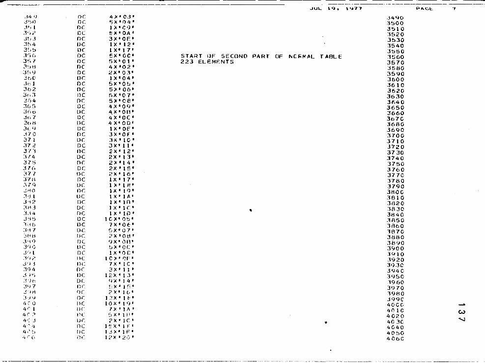
.JUL 19o 1977 P"-GE 7

.. 34 C) DC 4)CI03 1 3490 3')0 oc "5X 1 04 1 3500 -~·. 1 DC 1x•c9• 3510 3':>2 IX ~x•OA 1 3520 3!)3 DC 3x•or::• 3530 3'.->4 DC tx•12• 3540 3~-~~ DC lX 1 t7' 3550 :v; h DC ~x·cc• START UF SECOND PART OF 1\iCI'~AL TABLE 3560 3 ~-) ' DC 5x•ot• 223 ELEMF.NTS 3570 :'hU DC 4X 1 02 1 3580 :_j~,<) DC 2X 1 03' 3590 .3b0 DC lX 1 04 1 3600 3i: 1 DC 5x•os• 3610 362 DC 5)< 1 06 1 3620 ::;, ':l nc 5X 1 07 1 3630 3;)4 DC s><•oe• 3640 3G5 DC 4X 1 09 1 3650 .J<'>o DC 4,X 1 0fl 1 3660 31> 7 DC 4X 1 0C 1 367C 3t> ti DC 4X'OD 1 3680 .1( (j DC 1X 1 0E 1 3690 .HO DC 3X•Of 1 3700 37 l DC 3x•to• 3710 37 2 DC 3X 1 11 1 3720 37] nc 2X 1 l2 1 3730 ]74 DC 2X 1 13 1 3740 .37:) nc 2)( 1 14 1 3750 376 DC 2X 1 15 1 3760 377 DC 2X 1 16 1 3770 37/i DC IX'l7 1 3780 .. -i l q DC t)(•te• 3790 3~'<0 nc IX' tq• 380C J·.ll DC lX 1 lA 1 3810 3·i2 DC 1 X 1 lfl" 3820 :~HJ DC tx•tc• • 3830 :u4 DC tx•tD• 3840 J'l •j DC tcx•o5• 3850 -1d6 DC 1x•ot• ]fl60 :1•1 7 DC sx•o1• 1B7C ]IIH fJC: 2X 1 08 1 3880 3•1 <) DC 9X'01l' 38-:JO jq 1_) oc 5><•oc• 3900 3·-· l DC 1x•oc• 3910 ~~·J ;• [)( tcx•t;F• ]920 J' I J DC 7X 1 1C' 393C 394 DC 3X'11 1

39'• c 3j~ DC 12X 1 13 1 .Jqso =~ ') t' DC 9:0<'14' 1960 J<J 7 nc ~;x•t!'• 3970 .j' I H DC 2X'1i.o' 3980 J·l4 or: l::!X'lf- 1 399C ~~' 0 ()( 10X 1 19 1 40CC -4 (' 1 DC 7X 1 1A' I~ ('I 1 c (,.) 4 (' ;> !)( :, X' 1 IP 4020

"'-J ,,,: j DC ;;:>X I I c. .. 40 3C 4 ·' '• DC l~X'1f' 4040 ,._ , .... ~-, DC 13)<" lF' 4050 4 r· (; D<.~ 12X'2C 1 4060

--------- ·-----------------------------·--· ------------ -------- -· ---- ·-- ---- -------- -- -----------------------

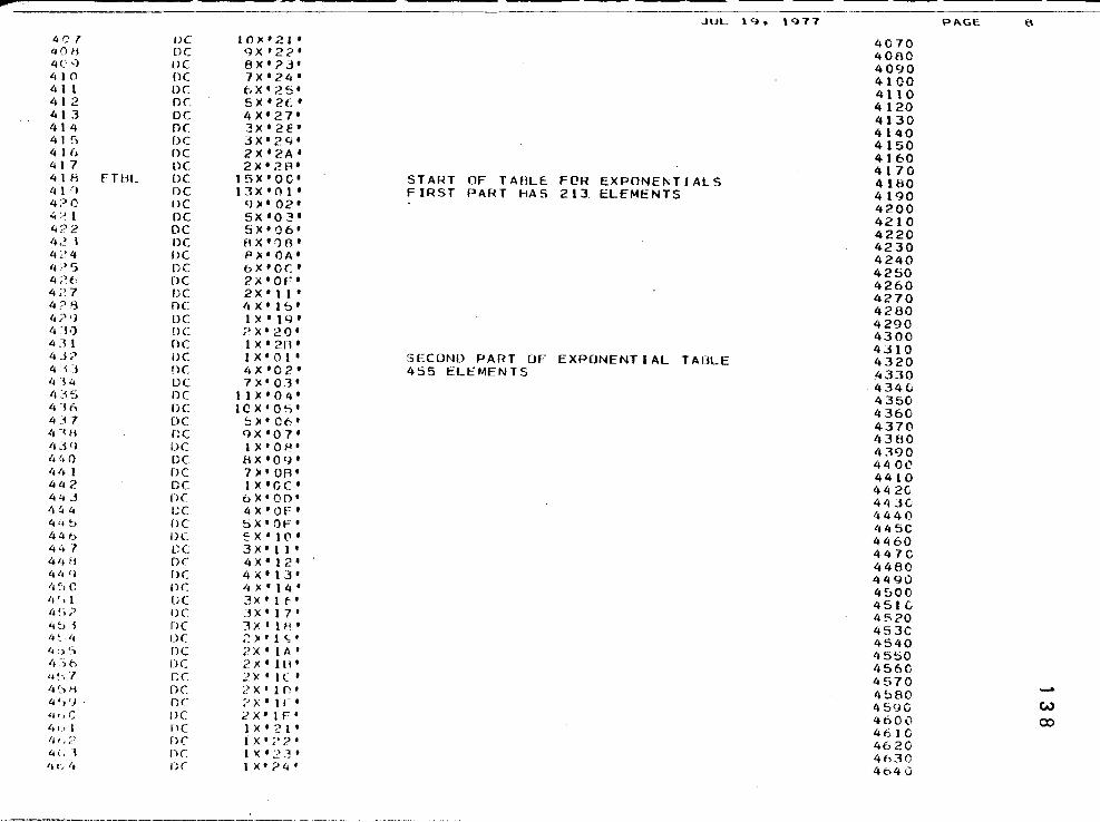
-----··--40 1 DC <~on DC 4C 'l DC 410 nc 4 1 1 DC: ~~I 2 DC: 41] DC , .. 4 DC 41 ::i DC 416 oc 41 7 DC 41B f"THL DC lj 1 q DC 4::>e DC 4;.:>1 DC 4?2 DC 4,! j DC ,, :• 4 DC 4 .> 5 DC 4?6 DC 4?7 DC 4?~ oc 4;:> ') DC 4 :l•) DC 4.11 nc 4..1? DC 4 -~] DC 4 ·s 4 DC ,, ~~ 5 DC 4 -lo DC 4J7 DC ~~ :l B r:c '13fl DC /j t, () DC ~~I~ 1 I>C 4ll 2 DC 4'1 j nc It 4 4 (;( 4 , .• tJ DC 44 fJ DC 4.:17 ec 4111! ()( 4lt q DC It~-, C nr. It r, I DC 4')? DC 4 t> ''I DC 4 :·. '~ IJC 41.) (::, DC ,,_--; h DC ,, ~- 1 r;c 4~~ H DC 4 1 >9 DC iJt J c DC ,,,, I i'C IJt1? f)(

4 (, \ nc ~~ L /~ I)(

10>< 1 21 1

9X 1 22 1

8X 1 ?3 1

7X 1 24 1

t>X'2o• 5X 1 2(; 1

4X 1 27 1

3X 1 2E' 3X 1 2Y 1

2X 1 2A 1

2X 1 2R 1

tsx•oc• 13X•Ol 1

C))C 1 02' 5X 1 0 3 1

ox•o6• fiX 1 00 1

P>c•OA 1

6X 1 0C 1

2X 1 0F 1

2X 1 ll' IIX 1 15 1

1X 1 }(.j 1

~~X I 2 0. tx•2n• tX 1 01' 4X 1 02 1

7X 1 03 1

llX 1 04 1

tcx·o~~ 5>c•C6 1

IJX'07 1

ax·o~· HX 1 09 1

7> 1 0A' 1x•cc• 6X'00 1

4X 1 0F' 5X 1 0F 1

!:X 1 10 1

3X 1 ll 1

4X'l2 1

4X 1 13 1

4>< 1 14' ::lX'lf- 1

3X 1 17' J X 1 1 ~~ 1

~><•ts• 2X'1A' 2.X 1 lll' 2X'1C 1

?x • 1 n • ? X I 1 ,- • 2X'1F 1

lX 1 21 1

1 X' ;•? 1

1'< 1 2.1' IX 1 ?4 1

JUL l<:Jo \977

START OF TARLE FOR EXPONE~TIALS FIRST PART HAS 213 ELEMENTS

SECOND PART OF EXPONENTIAL TABLE 455 ELEMENTS

--- --- ----------· 4070 4080 4090 4100 4110 4120 4130 4140 4150 4160 4170 4180 4190 4200 4210 4220 4230 4240 4250 4260 4270 4280 4290 4300 4310 4320 .4330

-434C 4350 4360 4370 11380 '•390 '~4 oc 4410 44 20 443C 4440 445C 4460 447C 4480 4490 4500 451C 4520 453C '~540 ~~ 5 !:>0 '•560 4570 4oAO 4590 4600 4hl0 4620 4630 4640

PAGE B

-w (X)

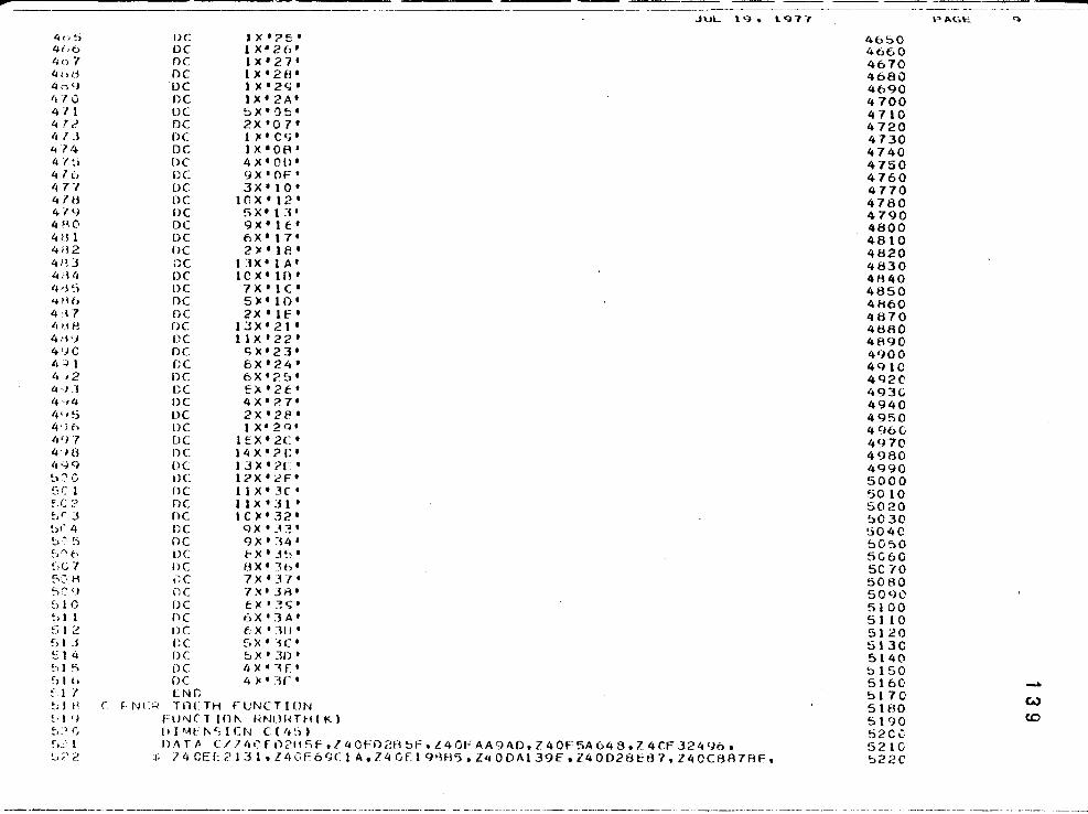
4o5 41 .. 6 4<', 7 4 t >lj

4n<J ,,-, 0 4 ll 47<' ,, 7 J 47-~

4/~i

416 ,,-, -, 47H 479 4 ~~0 41!1 4112 4n3 4.-ll• {.d ~~ qH6

4 -~ 7 '• tit! 4d'J 4'JC 4 ~ l '• 12 4•.1.] 4 ·ill /jlj 5 4'l6 ,,,,-, 4'18 ,,qq ~:c !.:,(' 1 f.C? t,r J !>~' ,,

~·: ~) ~-) !") t_,

~-,c 7 !:"""~·:= H !'>C<J ~'I 0 ~. I I ~_i I 2 !·,I j

t I '~ 51 ~~

~)I t> ! I 7 ~-I H (

! , I 'I t-J:) (j

~):~l 1 ! .. );:.) 2

DC DC DC oc DC DC DC DC DC DC: nc DC DC DC DC DC oc f>C oc DC DC IK DC DC DC oc r:c DC DC DC DC DC DC oc DC DC DC DC nc DC DC DC DC l>C DC DC nc I>C 1:c DC ()(

DC ENG

1X 1 ?!5 1

1 X 1 26 1

1X 1 27 1

IX 1 2fl' lX 1 2<; 1

lX 1 2A 1

5X 1 05° 2X 0 07 1

l)('CCJ' IX 1 0A 1

4x•on• 9X'OF 1

3x•to• lC'lX 1 l2 1

sx•t:~• 9X'1c' 6X 1 17 1

2>r'18' l3X 1 1A 1

acx•1n• ·tx•1c• s>c•1o• 2X 1 1E 1

13X 1 21 1

l1X 1 22 1

<;)(•23 1

8X 1 24' 6X 1 25 1

ex•2c• 4X 1 ?.7 1

2X'2P 1

1 x• 211• l~X'2C 1

l4X 1 21:• I 3 X 1 ?F 1

12X 1 2F 1

llX 1 3C 1

llX'31 1

10)('32 1

9X 1 J3 1

9X 1 ]4 1

f X 1 3~, 1

BX 1 3b 1

7X 1 J7 1

7X 1 3A 1

t )( I ~<_;I

6X'3A' fX 1 :11-l' ~;x•-sc•

o.x•Jn• '•><·~r· '•)<•:sr•

f-ND:J TI1CTH f"UNCTION FlJNCT 1111\ I~NIJIH~H K) I•I•.-Itt\SICN C('•~>)

JUL 1q • l977

DA T /1 C/ /4C f 112115f ,/40F02n 5F, L4 OF A.A9AD, Z 40F5A648, Z 4CF 32496, ~ 14CE~?l31ol4GF6gC1A,740fl9~A5,Z40DA139EoZ40028E87,Z40CBA7AF,

~·--------·-------·-- - ------·---·-·-------·-

----------

4650 4660 4670 4680 4b90 4700 4710 4720 4730 4740 4750 4760 4770 4780 4790 4800 4810 4820 4830 4840 4850 4f:l60 4870 4880 4890 4<)00 4910 492C '•93C 4940 4950 4960 4970 4980 4990 5000 5010 5020 5030 !jQ40 5050 5C60 5C 70 5080 50<;)0 5100 51 10 5120 5130 5140 t>150 5160 5170 5180 5190 52 CO 5210 522C

PAC.E. q

-w c:o

~2 _j

52,, f-, :<! ~) !_);> (,

~,,r,

~ ~~ H t~? <J ~)5 G ~) -, 1 b:12 f,~i .J

~' _i '• 535 ~.-16

~j7 1 ~i3B 4 b.3l) !.)'· 0 !:) (~ 1 6 5'•? ~14 j 7 !:)4'• "I ~~~ •:=; ~~~ 6 5·:. 7

, .. -~

54 i1 ~)I~ <)

~)~·C 5:,1 ~)':) 2 !.·'-,J ~~ )4 c :)~) s 5 1·\o ~)c, 7 f.J ~. tl !:)')'-)

~n. 0 fif, 1 ~If' 2 !"'f\ 3 !)t. '• ~.,(, 5 ~-)(' 0

~,f.-,

t)6 ti ~., ... ; ,, 7 f)

~' 7 1 <::. 7 2 ~) 71 !; 'll ~) I~)

~,-, 0

~ '7 t. 7 tl f•-, q ~.-1 c

- --- ---- ----JUL 1 <i • 1 <il77

$ Z 4 0 C 1 0 ? A f-- o Z 4 0 fl n F 11 0 D • Z 4 0 A C F 5 1 3 • Z 4 •) A ? F f.' 4 A o Z 4 0 9 A E 7 8 C • Z 4 0 '11 o 2 6 G t

5 Z4CH7~HAC,Z40705406oZ40734EODol4060C8F6oZ406lC22CoZ405A1Dl5o ~ Z40~?A7FFoZ404A32E7oZ4043AODOol403C28B9oZ40372~54oZ402FA03Do • l402AQCOEol40259Q7J,Z4020Q60EoZ401El45CoZ401910F7oZ40168F45o $ L4Cl40ClJ3ol4011BAE~,Z3FFOA2E4oZ3FC887BEoZ3FA06C98,Z1F785172o $ Z3F7B5172ol3F503&4CoZ3F50364CoZ3F50364C/

OATA ll/ZFHC3E4nC/oi2/ZFE79702E/ IF(t<,GToi1)G0 TO 3 S=Ur-.1(0) T=U,...I(C) U=AJNTC7.*(5+T)+37o*ABSCS-T)) X=UI\1 (0 )-UNf (0) HNORTH=.Ot:25*(X+SJGN(B,X)) IH:. T URI\ IF(KoGToi2JGO TO 5 RNO~T~=2e75*VNI(0) J=1f.*ABS(RNORT~J+l. J F { J- 1 4 ) (; o 6, 7 p;(J+J-l)*e1497466E-2 Gil TO R P=(PQ-J-J)*o698817E-3 IF (UN I ( 0 ) • G T • 7Q • 7AB4 6>~< ( E XP(- • 5>~<PNORTH •RNOR Tt-H

'f, -C(J)-P*{J-lfo*ARS(RNOfHH) ))) GOT04• ~f'TUHN V=Vt\1(0) IF(VoEO.C) GO TO 5 X=SGRT(7o5625-2o*ALOG(AilS(V))) JF(UNI(0)*X~GT.2.75)GO TO 5 RNOf:Th=SIGN(X,V) I<FTLI<N FNf> R~XP TOOTh FUNCTION f-LJNCT ICI\ r;EXPTH(K) Dlr...,ENSICN C(65) f>AT~ C/l40FOCOOO,Z40E10000,Z40040000,Z40C70000oZ40BROOOOo

$ Z4CAFCCCC.740A5000C,Z409AOOOO,Z40Q10000oZ40890000ol40800000o $ Z407A1000,Z4071000Col406A0000ol40640000,Z405EOOCC,Z4C58000Ct ~ 74~5300CCoZ404EOOCO,Z40490000,Z4044000C,Z40400000ol403COOOOo t Z4C1G0000,l40l50000oZ40320000o7402FOOOOoZ402COOOCol4029000C, J l4C27CCCC.l4G240000,740220000o740200000tZ401EOOOOo7401COOOO, $ l401AOCOO.Z4Cl~C000,740170000ol40160000oZ40l~OOOC,24013000C, t /4012JCC0,740ll000Col40100000oZ3FFOOOCO,Z3FEOOObO,Z3FOOOOOC, •f. 7 1 f C C 0 0 I' C , l 3 r IJ 0 0 0 I) 0 .1 W H 0 0 0 0 0 , Z 3 F A 0 0 0 0 0 t Z 3F q 0 0 ') 0 C , Z3 F 9 0 t'.l 0 0 0 , J, l .11 tiC C C 0 tl • 71F n 0 O') C 0, ll F 70 00 0 0 • l JF 700 0 0 0 o Z3Fo 00·) 0 0 o 73F 60 00 0 C , ·Ji 1 .! F 6 0 C 0 0 0 , l ::l F ~~ 0 C 0 0 C , Z ] F 50 0 0 0 •) , Z 3F 4 0 0 0 0 0 t Z 3F 4 0 0 () 0 0 , Z 3 F 4 0 0 0 0 0 / DAT~ ll/7fhtlfAA91/ J F ( 1<. • G T • I 1 ) GU TO 5 Ul=l.JN[(C) IF(Ul.GT •• 7gl7t;4<;) Gn fO 3 T:::J.-l.?JY'1n2>1<lJl I~ F X P T H =-A l CG ( T) J = l <) • "H F X F f Hi l • 1 f C U~ I ( C ) * { • C f> 0 I+* T + • 0 0 1 q ) o G T • T- C ( J ) ) GilT 0 1 f.FTL.HI\ HFXPTb=IG.?Ol5~*UI-15o20.1~2 J=lh.*hfXPlH+lo FX=CXF ( -fi[XPTH) I F C lJ N I ( 0 ) * ( , 0 l, (' '' '"F X + • 0 0 .l ') ) , G T • E X-C ( J ) ) G 0 T ( l 1

5230 5240 5250 5260 5270 5280 5290 5300 5310 5320 5330 o34C 5350 5360 5370 5380 5390 5400 5410 5420 5430 o440 54 tiC. o460 5470 5480 5490 5500 5510 5520 5530 55L~0 ~j!JbO

5560 5570 5580 5~lJC 5600 ~)6 10 5620 5630 5640 5650 566C 5670 5t>80 !:>690 5700 5710 5720 5730 5740 5750 5760 5770 5780 57qo ~BOO

p "'<:.\' \.()

-A

0

5'!! ~'.>-i? SR3 ';-,H '• ~:t\5

!'iM6

') Rt: TLRI\ lJl=UNl(C) IF( L.l eEO.CJGC TC 5 HEXPT~:4.-ALOG(Ul nE Tl.RI\ END

JUL 19 o 1977

5810 582C 5830 5840 5850 5860

P,._C.E \.\.

-A

~-----------------·-------·--------------·- ----------------

AP?mmrx B

142

1> 1~.4'J.J':1 .Jub *l~>.'JOo21 ,JUit 1>)~.•]0.4::\ .JOU ~>1~.'>1• iO ,.liJI.l 1>}!;).<;).4!:1 J(Jtl

't.*l~.~l.4'J ,1()11

711 7fl ffl Ill If! 171

H A S f'

-- HAlhfAt2 -- B~GIN~I~G lAtC - PAHT lJ lLUOUll HAltltAC~ ASM l50K HEQ, lLUOhll HA ~FAC2 fOHI 501< HEUt TLUOU}l H~ldtAC2 LKfU l50K HlUt lLUUO}l HAIHtAL2 00 150~ HEUt ·- HAlntAC~ -- ENU EAtLUllUNf 973

S Y S 'f E M L V G

• CLASS 1 _l50K USEDt

AOI< USFO, '16K USEOt 3HI\ USEOt

1-lNFS

381881~~ ~f: 8818818~ ~~H: OOIOOI~b ETt 00100101 CPUt 00100115 ETt 00100103 CPU,

!l:~n: lo55iit

C!6o09iit

8888 0000 0000

1~8~~~ CCOHP) CCOMP~

HA~PJolol4 JUH ~IAllSilLS -- b50 CAHUb kfAO -- 9db LINES PRlNTED 0 CARDS PUNCHED -- lobO MlNUTtS IELAPSEO TlMtl

-~

w

IIH•'ihf!>LO( Jllu 13ltJlt1tt21t'MilLlf< 1 t II M~GltVt.L;(},!ltCLAS~=ltfiM£:1 /I FXtC I<~MIJI Of< I tf'At-<~lell(tll"'

XXI'S~bftHH f'KIJC Ut.CI\:1 I xx~SM lxtC P0M=AS~GASMtP-kM='boLOtE~tRb•UMtfXtcU=3t~DEC~t

lttb~il SUh~TllllllON JCL- P~M=A~MAASMtPANM~'HtlOtEStHLt M~fXtCO~J,f - " .O.SYSl!ti OU (;:,~:MA1Hcl0.~1ACL IBtDISP=SHH AX litl USij::,YSi•"·ACLlbolll SP:SIIR AXSYSUl I ~U UNif~SYSI1AtSPACf=jl~OOtC4UOtSOl) XXSYSlol2. lJIJ lJN) =SYSOAtSPM:t: J500t 1400,50 I. ~x~YSU13 UU UNll:SYSUAtSPACt:(J~OOti400,~0ll

IISYSf'l<fl-11 IJil l.lUi'~lY XISYSPR!Nl UU SYSOUT:A X~<; Y SPUNCri IJII S Y SOli T :11 ~-. ~--- - . XXSYSLll~ liu.USN=~LOAOStToUNll=SYSUAoSPACt:l80t(200t~Ollt XX UlSP=IHGlltP~SSltOCb=IH~CfM=toLRECL=bOtbLKSIZE=801

IIAS~t,S\S!Ij llll " ltt23bl ALLOC, fUh NAIDtAC2 ASM lEf~J/1 2~1 ALLOCAltO TO SYSLIB Jtt?~71 l~O ALLOCATLO TO

f tti~/~ 1~7 ALLOCAltD TO tf<.'J7 1~5 AI.LfJC.ilft_i) 10

Itt2J7l 1~7 ALLOCATtU TO lt~~31l JC1 ALLOCATED TO Itt~J/t 1~5 ALLUrATtn TO Ilt~l7 3~1 ALLOC~TEO TO

SY~UTl SYSLil2 c;vsurJ SYSPUNCt1 SYSI..lt'i SYSIN

lltl42l - SlcP WA~ tXfLUltU- C~NU COUt OOnO It.Fclbl M4Hic}O,MACLlu Jttio~I VQL 5tH NO~~ LOlOOlo lt:fctbl <;yS}.~;AC.Llti . lt~~b~l VOL 5tH NOS~ SYSVOL. !Et?d5l ~~S17~~1.1003~50.RFOUOokA18FAC~·R000307~ Jll-2!:1~1 VlJL ~.tH ~lUS= Lfl3031, Jtt;H~l SYS7/~~f.TOOJJ~0.Rf00ooRAlAFAC~oH000307l IH'?tl':>l VOL ::.LH NUS= Ul3029. . ltt~U~l SYS712~7.T003350.Af00QokAl8fAC~•R0003072 ltt2M~l VOL 5tH. NOS= L&303lo ltt?n~I SYS71i21.10U3J50.RFUOOoHAlAFAC2ol0AOSET ltt2b~l VOL SLH NU~= L03029.

llt.!/Jl 'ilh' lt~~t'l I Sl4i-'T (7,~~-I.J':J't~

J06 17l

00000100 OOOO!l200 00000300 00000400

88888~88 00000700

88888~88-XOOOOlOOO

00001100

KEPT -I(£PT

DELETED OELETEO

UfLETf::O

-PASSED

J LIIIJ o);> I 1 I I tOil? I li 11Ufl21 1LII(t021 Jll1Uil? IL"JOcT lllll!(li:'l lLIJVOd JII•(IOJ I

H~1/td Slf_p 111:;iM I SlOP f7?.i'c7.l:.!:IO CPII S 1f I' 1-.~)11 I Lii~Il 2~1 4 i: l(l..f•S

OMlN 06,3'7SE~ MAIN ~~OK LCS UK

<;tFI' //1'-,M 1 UrH I 1~0 ?iJ tXL:PS Slt:l' /.U.~>I-1 1 UIHI ~~-, 0 EXL.PS ~ltf• IASI1 I ll''lll !!:>5 lV t:..<l.f'S SfU• IA~tt I UNl I 1:)7 i: [ALI-''i '>111· /AS~· I l•Nll JCl 0 EXLPS SHi• /ASH I IJiHT ~~~ )~ rxcPS r;rt~· IA~;M 1 ll"<lT Jt>l ~1'7 txu·~ SIU 1-.~~~ I ti(Cf'Sl Ul!,~, Ill; lAPE

AKtl.tfll L.-.t:t: t--IJt·•"ltHOPl•~-'AI'M='Ll~lr.on .. co• K).~I'St'Hlt~l' tJIJ ::.YSOtll::A 1\;~SYSPtiNLtl Uil Sf~}l)Uf::IJ )I,,SY 'iL lf~ IJLJ IJSH::t~,L;;AnSFT tld SP"' lh\lUtPASSl t J\ 1\ 1J l- b = lli t C t t:::. F t L fl t L L = o 1l • I • L r S 17 t =II ll )

/I~Oilf.',tSlr; vf• * H t .~.lid fiLl til,. r ()h l--Id l!t IIC2 ffJfH !H2:j/1 HJ4 i.LLilCI<lLll TO SYSf'ldNf lttcJfl JCl 1<1 t.rJC:,•lt.l) 10 ~.YSI'uNCt1 lth'Jii l~)'> ,,, LUC1dl1J TO sv::.LTN

ll ~ I ,, I. I - s l t t· , r'. s I U:.: .II! l~4 ALL tl('\1 tfj 11'• S Y ~,( 1'1

< I'.LLu Ill! - LU<W l.ll 11t. OIJIJ(J

01 IJR ~1'111 TP 01 00001200 0(1001300 0000}400

l\0000 suo 00001600

TOTAL 6001

-~

~

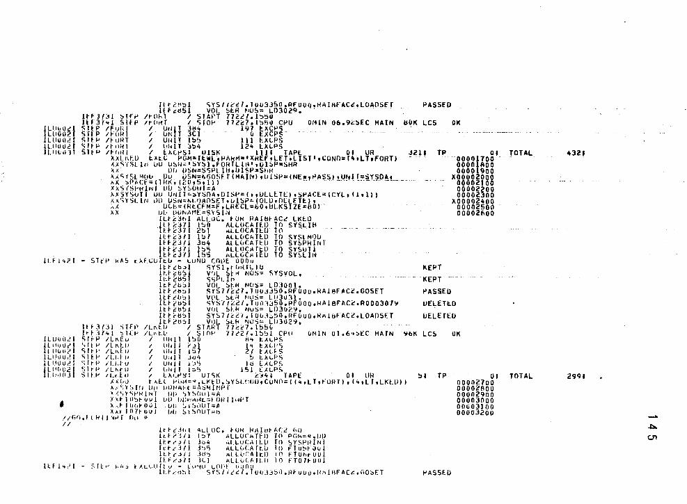
ltt?~~~ ~YS/Iii7.1003J50.PfOOQ•HAlR~AC~olOAOSfT lff~d51 VOL SER NO~= LD3029, .. . . .

HFJ(:::Sl ~lfl-' /tOhl I SlM'T 772cf.l';)':3U

PASSED

I LIJldl c l lll0021

ILliUil~I H.llll02J JLIIIJ 0] I

Hf31'+1 Slfl' ltC•tfT I SfOf' 71U7al~!;ll CI-'U SltP /fuRl I UNIT 3~4 197 I:.XCI-'5

OMlN 06.9~SEC MAIN b~K LCS OK STtP /tOW I UNIT 3Cl 0 EXCPS-SltP /tUMT I UNIT ~~~ lll EALPS ')lfP ltlltcl I l!l~lT ~~4 l2<t EXLPS SHP IHJtll I t.J\(1-'SI UISI\ llll TAPE 01 UR

XXI ~EU l~t~ PGM=ItWLti-'AhM••XREftLEToliST'tCONO=l4~LT~fORTJ AX~YSLlri UU usw~•SYSI,fONTLlri'•UlSP=SHR XX Of1 USN=SSPt llloiJlSP=Stof< ~f;!~~~r!r~ CT~~' ~~~~s~Y?fF I IMAJNI tUJSp;(NE~pt>A~~) !U~H t~~J.~D~L _ XxSiS~HlNI UU SY~OUT=A J\XSYSUTl UU UHIT~~Y~DAtOlSP=IttULLETEltSPACE=<CYLtlltlll ""':;YSL IN lHl USN=~LOAO~ETtUISP=-IOLUtOLLF.TI:.I, ~X ULb~IRI:.CFM:F,LRECL=&O,ULKSIZE=BOI. XX uu UU~AHE=S,SIH

ll:.t2Jhl ALLOC. tOH HA16tAC~ LKI:.O

f lt~Jll 1~0 AlLUCATtO TO SYSL{H ~·~371 2bl ~LLOCATEU TO llt~l/1 1~7 ALLOCATlU TO I•t2JJI Jb4 ALLOCATtU TO

l ~ttJ71 ~~~ ALLOCATtO TO t:t2JIJ 15'5 11LlGC1-1Tf:U TO

ILF I'll' I • 5TtP l'ii\S t..>.f.i,;LJTt.u - I.IJNtl (Ollf. llOOol ltf~b~l SYSl.t~~fLIU

SYSLMOIJ SY~PkiNf SYSUTl SY~LIN

ltt~USI V~L St~ NOS= SYSVOL. 1L:~2t151 ssPLlri lct2b51 VOL S~H NOS• L03001. ltt~o~l Sf57f2~7.TU03J~O.RFOOOoRAI8FAC~oGOSET ltfctl3t VOL ::.tr~ ,,,US= LIJ311]}, lltcUSI S~S71~~1.TU01J50.~FOOOoHAJ8FACc.R000307~ ltl-cb51 VoL su< Nus= LD3ll2~. lt~~b5l SYS71~21,10~Jj50,RFOUOaHA&ti~AC~.LOAOSET ltFct!Sl VUL St.h NUS= LU30!~.

Itt31JI STFP /L~tU I Sll\kl 77~£'7,}55U

~2H TP OJ 0000f700 -0000 ROO 00001900

X00002080 . -- .. 000021 0

KEPT - -KEPT

00002200 00002300

X00002400 00002500 00002f>OO

PASSEO

UEI,.ETED

UELETlO

I t t :i14 1 ':: I L P I Lo\ t l, 1 S I n ~ ·n t' 2 l , 1 55 1 C I' !I liMlN Ol.6~!>EC MAIN Slt!J ILKEu I tlf~ll 1~>0 fl<t LJ(I.f'S

~bK LC~ OK ILUOO.?I

tL•HJilc 1 I Ill! U! I

I Lilli u ,• I ll IIOtJ,>l

f L t q, u ,:>I 1.11·1031

•

ql ~ ILKUJ 1 told I t'.J} H l:xU~'i Sltl• /LrdtJ I lil•lf &57 21 fAll-S Sift" /Lt,I·IJ I lJ•ill Jo'• !:. l:.l\I.PS <;ftP /Lht·u I lJI'lil 1:.>') lb t.ALPS ShfJ ILI\tiJ I ld<ll 1!:>5 I'll tXLPS Sit!" 11.tT11 I tJ\1.1"~: UJ<;K :C:74; lAPt: 01 liR

J,.;c;v t>.H t'iii~=·•.Lt<t£l,:,Y~l.t10UtCUNI)::((<t,LTtfORTltl'+tlftLKlUII Ar'oYSlrr lJ11 lJI)~•AI•:t=i\!>~H!PI" ~ J,<;y<;f'H 1,_·1 ll[l ',Y~IiUl :oA 1 '~ lll:,t uu 1 lJll IIIJI'!I\r•lt.::;l Clfi lli<PT XA~IOt,fOUl lJ[; ~.~>lllJl;jl X;.l· IOlfOUJ lJIJ SY'>I)iJT=Il

//C;O,IlRII'W[ n,, * II

lt~c'Jid ALLOC, ~Uk 1<11l11~M.c (,() ltti':111 1::>7 >llLUCATfl} TO PGfvo:::<~.lJU lt:t-,-,:~{1 1D4 ~<LLuC.\flll fll ~YSPidNl Id,·:J/1 J~,,;; >ILL!;C:AfUJ In Flu:'>IOLol ll ~ ( .,, j .i th A I L l• r. A I t_ll ff' f T 0 t>t u u 1 l~f~.l/1 iCJ ALLutAILO 10 fT071UUl

r.~.~:.cu It. •J - (w~u Cfll•t v.1nv H. r <' <J ~ l S Y S I l e! c l • 1 0 fJ .l3 S 0 • II f u u 0 • I lid ll FACt.: • C. 0 ~F.: T

ltFl•~l - STt~ Wh~

!ll TP

t'ASSE.D

01 00002700 00002AOO 00002900 00003000 00lJ03]00 00003200

JOTAL 432t

TOTAL 299t

-.c::.. (Jl

0

~ 0 .::l

"" cu-1-W

VI ...1 u lAO ...1 -o ,. ~ ~ :0 4 .. ., z <( 1-X t.J

u ~I!? u ..,j -c: !oi ·.n . .,. "

_,...., .... ~ ou <U . <(

f"l ~ :» 0 :I)

;;: 0:: z .... J:: .... '£ . %:

"' 0 ::> 0

..,;..:. . .... ::l.W.-1'1 :::: <IQ;I'l

~ => ~ ,_ ·~ ..,

r.,; Vl "'"'IF> VI 0~ U' C\_~CL~.:.. -r.!:l :=t ..... -...J...>~~ J ...... .,_J.3'.-.

.nii'><><><><X=><"l 4".(t rt.n..n..u..t.Jr..oJ..;~ Cll.ll.l'l ·.J)-- .::::.,n .... _. ~ • •00,."\,1:\,~ t--:: .. z~,..., ~

. ,,_,..... ·" '\1

0 .... <\.1,"\1 ::;"\\N "\J:t:"JN ....;._r- \I...Ur-r-J:- ...... -:..n--~ .... .,Jt- ~..n....J.-·::::'(;4 Jt>'='::t~ :>ere -t~~><rC

tf"'V),.....-:4"·r...r-- iJlU"l J"'f .c f) l);..J _, ,_r")....,,..,,"f') .• _._,'

.1' Jlr.<4"1.:"J:'\I ~ ._ ___ :-:..:OJ:.;.J...J ru _ _._. __ ...;.:v.~.J~ ~ (J.. ZZ~ZZ<~•~•

Jrr..l :,:.,j.=~:l.=.~..&J..J..O:>

::>'::) <r.<;: ;,::.!)'-''-''' .l:.X ,..... ..... ...... 'l.~ ::J:C !..Lu.. C'::::>

!J,lJ': ~o::.:::::::::

~-·!).!):!I'.!'!):

..,..,

~ ~'-'-'''' .. "'lD

~r"'l~'l.:J.:..r..~ -"J,'f1 .;_....,;,.ww.,;..6.1.,.:._;...,.. ......... .U..L.r-~~-.-~ ~ ... --(,/j~rJi(/'HJ);Ji -............... ~-

"\J"\JNN":'\!f9"+

~.:;,~.;, ,:)..,:)

==::::::-::.:: -...J-.J-!-~ _ ..... ._. __ ~

1 4 6

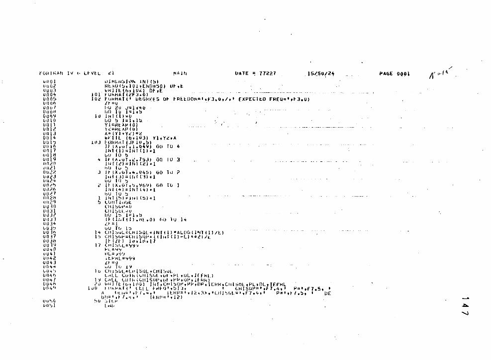
fUHI~~N IV b LfVtL ~~ l'i/.ltj UATj: ~- "/1C.?.7. 15~~0(2't

lJPOl li (j(i2 tJ u u:1 0004 000~ 01)1)11 I) 00 1 oooti (It) I] ':I ll<ll (J uo Ll OO)i' U013 0014 OOI'J Ulllh t11Jl7 llll 1 B 0019 011,'(1 lltlt'l oo~?. (JI);>J uu24 IJO!'':> U1l?.h UUt'7 !lll2H u029 (J u .i () 0031 (Jl)Ji' UI)J] ()()J4 (, 0 j~' UUlh UOH llOJh iJU19 uo-.o vU4l Ui142 0043 L•O '+"' ldh ., Ull4h (I(} 4 ' U04H ()(149

Uu':>u 0 I)~) 1

ul~lLI~!:>JllN !NT (5) A~AUI~tl0lt[N0=50) U~t~

tot ::~~~;~f~M~~b,oF.r ------- ------·· 10~ fG~MAll' UtGRFES 0~ tRllOOM=tofl,Otlt' EXPECTED FREU; 1 rt3oOI

Lr=u I•U ~u ,J=l tltO 110 l u I= l • ~

1 o 11~ r 1 11 "'o IJU !> I= lt 1 ~­Yl=KtXPIOI lL=HtAPIOl 1\=IYl+Yc')~>~ wF I It (bolUJ) Yl tV" oX

111J t lll<i~l\ I IJ~ lU,!::Il H IX.ulo1ob41J) Go TU 4 !NT ( ll ::JNl II) +1 bU 10 ~

'+ It-ll< •• uT .. .!.753l GO JU 3 )IJ I ( t) :: 1 N l ( 2) + 1 ,_,u r u ~

3 It IX.uTo4•045) GO ld ? ltjl (,j)::Lfjl ('3) +1 uu T iJ 'J

~ U IXollT.'J.':I6':1) GO TU INI l<t):)NT 141 +1 ,,u ru ~

l 11~ T I !'> I = 1 t-i I I 5 ) + 1 ~ UmT1tlllt

CIH~uP=I• Ltil ~llL"U IJU 1~ !=lo!l JH1r.TIII ·•~E.Ol c,o lu 14 Lt "1 GU TU l !l

14 CIH:O.tJL.;;;Lt11~QL+INTlll*ALOGilNTlll/t) 1 <:> ctll':>••~·::etiL::.qt•• c 1 ltd 11' -u G<>2ltt

Hllt-l lt!dtlol1 17 (H! SI.L='i'i'l

I"L"'-1'1 IlL" J'1'J lt.h1L='19'1 Lt :::\) ou Tv l'~

lu Ut!SUL=Ct1l!:illL+CHISuL L•li.L Llllld\..tilSI•l tlA of-l oUloifff<Ll

1'-J (I•LL LUII•iLIIlSIH'oiJf .~·PotWoHRk! <'ll ~Hi) rt IIJ• ltlOI ll·tfoCt•l::.lli-'oi'PollP,JU!I-<tCtd:;nLtPLoOl.olEFHL

luO lt'hl•'idl' ltt.L frlH.l'o!.>I:.lt t LHISCJf':t,f7.'"' t'::ot,fJ.S, ' A !Jto~'"'•l·l ... ,t ltHfl='dl:o'!:.,•LH!':li~L=••F7.'"' P::ot,tfo!>t I OE ll t I= ' 't I • '" ' I t:IHI:; ' I 1 i? I

'J(J iiLI--I.tHI

PAGt: 000! N"·'" /

~

""-l

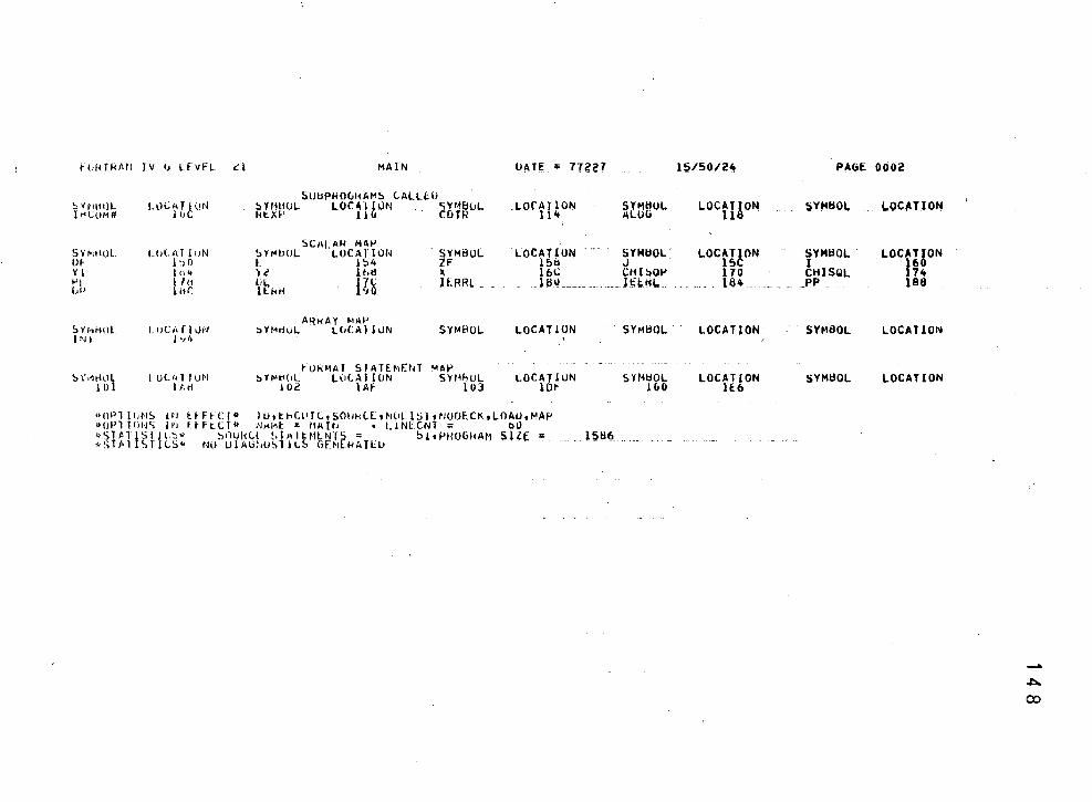
f~,fiTk/ltl JV I; LFVFL .::1 MAIN O,IITE "' 71?~7

5UbPHO~HA~S LAlltU ~YHtitJL Ll)C~Jt(tl\l ~ l'l1bOL. lr'COMII 1 IJ kt.Xf-'

LOC:41lON 1111

c; 6'~bliL. C Hl

.Lorn!o~ __ u~~(Jl.

5 Y ~IHI)l LOCAlltJN SCI\( AH M~t>

5YMbOL .L.llCA TION SYMBOL LOCATION -- SYMUOV Uf 1 ~) 0 l 1!:14 ZF l!>il J Yl lt.4 )~ lt.d l\ _ u~ _ __ __ .... ~2t~~ .. 1-'1 I f t1 li!.. H~ llRRL . (JP lhf. llkH

SYHI-Wl. I.<JC11 f ll.HJ Al'l~AY ~tAP

~YHduL LGCAllON SYMBOL LOCAT toN SY1'11:i0L I 'II I.._, it

tUHMAl SIATEME~T ~AP 5Yo~thll l UC!d TUN ~YMI:IOL L (I L\l I (JN S'n~h.OL LOCATION S'f'MijOL

I 01 1At1 102 lAf 103 lOt !GO

uoPlJ<,NS ill UFt"CJI> l.I.J tl: MClt J C, SOttklE.: t Mtl 1:; 1 , NOOtCK t LOAU, MAP ~>CJPllON'-i 11'1 Uft.Cl" i'l>\1~1:. : 11A lfJ • Li.NECNl :: oO <><;TIITiSTfl.~" ~-Sl/•1 Sl CS"

~nut~lt ~.flllt~ll.NT( = Nil UlAI;~,usltl..!:. GUt .I<ATEIJ

~l•PHOGHAM 5llE c ..... 1586

15/5012~

LocruoN

LOCATlON lS 170 164

LOCATION

LOCATION lf6

PAGE. 000~

SYt4BOl. I.OCATION

SYMPOL LOCATION I 160 CHISQL 174

_ .. __ PP _ 186

SYM60L LOCATION

SYMUOL LOCATION

-A

00

f OH T f< M! l V 1;> l b r!. t: 1 ~1AlN , IJATE = 11~?7 15/50/24

vool 0002 ooo3

\Jf)04 01)0'5 no 01'> ono7 (iO'l~ l/111]'1 (!()]()

UOll 001? \) 0 1 :1 110]4 00 I'> Ull]h 1Jill7 Ut) I h liOl'-

Oil<'fi lh•21 uvci' UJ?.J V024 vU2~ IJ ll?. (, 0027

C KN(Jti I 00111 ~ l>fjC 1 l ON fUNCfiON k~OKTHIKI

_i ..

I•

0

b

1

U!M~N5!0N C(451 . . . IJ~IA C/l40fO.:R~ft740f0?U~Ftl40FAA9AOtZ40FSAb4dtZ40F3249~i-

i t40ttclJltl40lhYC!Atl40ll~~H5tZ400All9EtZ40028f87,L40C687~Et i l40LlLiAbt740UbfUIJUt740ACt51JtZ40A2lE4AoZ40Y8E780tZ40Yl6l69e i t40til~btUtZ•07U54~btl40734lOU,Z406bCUF6tZ40hlC22CtZ405AJUl5t $ i*v5cb7tLtl404ijJ2L7tZ•043AD00tZ403C~d~9tZ403J2554,Z402FA030t t L402M'1CIJUoZ~0259~73tZ4020~bO~tZ401El45CtZ401910F7,z40lbdf45 1 \ L40l~OOY3tZ40llbbEOt73Ft0A?f4tZJfC881~EtZ3fA06C98,ZJf785172e 'Llt18Sl/ltZlF~03b•C•Z3F~OJb4Ctll~~Ul~4C/

UMlA ll/ltuCJ~40D/ti~/LFE7~102F/ It I K. (, I • I I I GO T ll 3 s;;ur~ll (!) f=UNl(lJ) n~A1Nl(I.*IS+TI+37.~AAbiS-lll X==UNllui-Ui'll 101 h"0ttlt·t:o.(Jt,;::t;,o (X+Sl~;>r~IJ:<•,<J I kLTU~N It 11\ol>f..!<:IGO ftJ tJ k•~llrd N=<' .lt~•VNI ( 0 I J;)b•*hh51HNORTH)+lo It IJ-l'tl 6•6t7 P=IJ+J-ll*•l4974t6L-2 (,0 rtt tl P=!b~-J-JI~.bqH611t•J 1t ltlt\lllll .t,f • J9o76b4b* (tXP (-.5•RNOiiTfl*t;NQRTI:I)

~ -l(J)-~*IJ-lbo*A~SikNOkTH)))) &0104 HtllJhtll v::vr.I 1 o 1 It !Vof-(,.(j) CoO IO ~ x~SQ~J(J.5~2~-2.aALUb(h~b(V))) ltiUI'<i!O)*A.I>To2o/t>lu0 fO 5 fmOHTh=~I vf·, ( x, V) t;t flJf<N LI'<U

5180 5190

~ns 5220 5230

~~~8 5260 5270 5288 529 5300 5310 5320 5330 5340 5350 5368 537 5380 5390 ~:yg 5420 5430

~~~8 5460 5470 ~41l0 ~490 5500 5510 sszg 553

PAGE 0001

--A

co

f0~TNAN I~ b LlVfL 0:1 HNOHTH IJA TE "' 77Z27 15/50/llt PAGE. OOOZ

SUhPHOGR~MS LALLED SYI1d01. LOLli I I UN SYMI:IUL.. LOCAllON . SYMBOL -· LOCA~~Oill ___ - _ ~l~¥1JL. ___ LOCA[AON. __ _. f~gsoL LOCAHON UIH IJ't Ill• J l!tl L\P

lQUIVALE~Ct ~~iA HAP lOCAl ION - ~·:- ---- S'rHliOI.- - SYMBOL LOCATION ~YI'itltll LOLATIUN S'rMt10L LO<.ATION SYMBOL LOCATION R~I(JtHh JJtl

SCALAR ~1AP ~-~~---". -~ ....... - .._. __

SYIIH\lL l.OLATluN StMt1(JL LOCA f !UN SYMUOL LOCATlON SnltiOL LOCATION SYMBOL LOCATION Jl J JC It! l<tO K l41t s 148 T l4C b bl)

"" 1!>4 .J l5tl p 1St v 60

A>H~~ Y MAf' SH1lJOL LUt!\1 I tiN SYMbOL LOCArlON SntBuL LOCAUON ______ SHilWL. _____ LOCATION. ___ SYMBOL LOCATION L !b'+

t>OPT lll~'S IN tt-f't.CT" ll.lti:.IJLOILtSOIIHC:I:.tNOL[SI fNODE.CI\tLOIIU,MAP ~>OPI fONS iN li-H.Clit 1'4iH1t ;;; NNI'\IHti t I IN C1'i = bO ' QSTI\ll~TICS* SUIJNLl STATIMt~lS; 27tPHOGRAM SlLE = 1368 t><:;fiiiiSliL'>" NU uJ,\(JI<O':.liCS ufrJERAH.IJ

-CJ1

0

fURT~IIN IV h LEvtL ~~ 1-11\lN ~'ATE :a '!7??7 . l~/50/?it

uonl uoo2 uoo3

uoo4 uno"> IJO (If, 00117 UO!Ifi uoo~ UUlll lJ Ol l UOI? tiel 13 01114 UOl"> Ulllt> liO I 7 uOlti U<ll'i UU20 (J !121 U!lt'i?

c

J

...,

H~~p lOOTH FUNCTION ~UNLllU~ Ht.PlHIKl O!Mf~~lUN Ll~~l . UAlA CtL~UFOUOOOoZ4UElUU00ol4D04U000tZ40C70~0~,z~ORHOUOOi

t L~u~fUOUUt/40ASOO~Ut740~kOOOOoZ4U~l00UOtZ4Ub~OOOOoZ40&00000t 1 L4U(h00UUtL•07lOUODt740bAOU00,74Ub4UOOOtZ40~EOOOOoZ~0560000t ' L•U~~UUOUtl404fOOOU,74049U000,74044UOUO,Z40400000,Z403C0080' i L4uJ~UOOUo74015UUOUoZ4Ul2000UoZ4U~fOOuUo2402COOOOoZ402~00 Ot • L4021U000ol4Ul400UiloZ402~UOOUo740200000oZ4UlEOOOOoZ40lCOOOOt \ L4UlAUOUUoL4UlVOOU0tZ4dl70~00o740lbOUUOtZ40j50000tl401JOOOOt 1> l41) 1 'o o o o' l4 o 11 o u o u, 74 o ~ o o o o o, l3FF o o !i o o, z 3~ to. o o o no, z Jf ll o o o o o, ~~ .. ~ ) LJftooouOoZJFrtooooOoZJFBoonoo,ZJfAOuboOoZ3f900000o23FYooooo, ) L~fbllOOU0olJfHOOOOOtl3t70UOOOoZ3f700UUOt73fbOOOOOoZ3fbUOOOOt i t3fbOOOOUtZJFSd0000oZJfSOOPDOoZ~f400DOOtZlt400000oZJf400UOO/

UATA ll/Z~b4fAA~l/ HIK,GT.l.liGO 10 !:> lll =Ut•l I(; J lf1UJ.GT .. J'H7049J Gu 10 3 T~l,-),~3~~62*Ul lit. ~Pl tl=-illUr"i ( T I J=lb,<>f.<E.APlH+l, H llJ~,J IU)<>I,0604*T+.0039J ,uJ,T-CtJl lbOIOJ kt.{IJkN Ht.~~1H=I~.~Ul~~*Ul•lS,2Dl!:>~ J"Jb,llt(f.Af'IH+l, tA=tAP(-htA~lH) . I~IUhliUl*I,UhO~*(A•tOUJ~l oGT,EX-CIJllbOTVl H~IUHN . U!=liN!(O) lt IUlotiJ,Ill C.O TO S kt.APin=•··ALUGIUll HL lliiul I:. I~ II

5540 5550

~~~8 5580 5590 5600 SblO 5620 5630 <;640 5650 5660 5670 5680 5690 5700 5710

~H8 5740 5750 <;760 5770 5780 5HO 5800 5810 5820 5830 5840 58~0 5860

PAGE 0001

-(.TI

fi.J!IHUIN TV b IX\IH. cl Ht-<PTH UA TE '" 712?1

~Ut!PHOGH.~<M~ LAU l:.ll ~YMiiOL lllC~flllN :,HJtJUL LUCAllON 5 Yt11HJL i..OCATION UNI 11, A LOu t.:ll fAP C't

~YNti(Jl lUUIIlliN SYr;HOL k~ >.PTH tfl

lUU IV II.Lt.r~r:t f.JA 1 A MIIP I..OC" flllN SYMHOL LOCATlON

~CALAI-! MAP ~YI-IHOl l OL ''I l<ll\l ~Y~ItlOL LOC.:A I I IJN SYMBOL LOCATION 11 t.C: t, I Q IH Ftt 1:.)1 10 1)

M~HAY M/.\1' ~ ~ M>Hll LIJLIIlJUN :lHJl>OL LOCATION SYMHOL. LOCATlvN L IIH

"iH'l I IW~; ill U' Ft.C fil l U, t:.t1C.:LJJ C, SOUf'lC.:b NOLl~ It ~UDECI<. 1 l.OAI.l 1 MAP <>OPTION'.; 11~ Etfi.CI* IJ ... Ml ::; Ht.X>-Tr1 t l.INE.CNl :o 60 n<;11111511LS•• SOilliCt Sllllt•II-.NlS = 2ctPHOGkAt1 SI/E • 1076 ~>Sl ••T lSllL~" h() I.JlAiii··OSilL::. i.ifHI::kAlEu

<>~l1lTI~llCS" 'JO IJIAb1WSTILS HilS SIH'

15/50124

SYMbOL LOCAl lON

SYMIJOL. LOCATION

SYMtjQL LOCATION T f8

::iYMBOL ·- .LOCATION ··-

PAGE OOOZ

SYMBOL LOCATION

SYMBOL I lOCATION

SYMBOL LOCAHON J

SYMBOL LOCATION

..... CJl

"'

..I V'l

<I _ .....

"'"' !"-C -4:1

wCCC ZN._ :>· zo~

>D·.LI .-.o :'\I .::I

CC'<I ..;­...... ,.z ..... u..:..u -.....:-.....~ ~ ..... :x:; ..._~

~ If)

tJ'; "" I :C tJ'; ::::;:,­~ .... :> -..r.::l '-:> .:.. .... :>-n

.n­J:.-< .:;.z..J --:> .::.>-0 .,;~..!

0 .LI .n .=;-......: -=t....J":) :s:::-=~ .?<::. _,._ _ _..

~ ..... > z .... .... ~ « I 'Z

.JJ ~ - " " "

1 5 3

~ =-It II

Q

1 54 It a: a: :r a: a: a: w w w -., .() N ..,

"' N 'XI :u ... . . . "' 0 0

I II Q

z z z w w w 0 Q Q

''-\

I '·--.. Q

M • "' -. (I)

' ..,

;\ M I N ..,

.. ... ' ' (I) c •

i . . 0 0 0

• II II 11. 11. C1.

., ... N • lO "' .() 0 ., G) • ,..,

N

D 11 " ..J ..J ..J I 0 0 ... \ ..... en (/) - I ... ·- ""' :r :r .., ~- ~ u :J <'

_,,

0 rr. :r u -· - ·-.

"i ""'· 0 .. ::0 0

.. '\ ~ t\ " II ... :X a: ! ... a: a:

• .. .... w w "\

" .:r C! ILJ

... ___ , , .. ~ . ,-:, ,.. -,....._

...._ ___

.----...

.-.

+

,... ~ r-

"' .., (0

0 ,, z ~ Q

.;t N .;t .c o'\l

0

" :I.

0 0 ::> "" " .. C1. 3 ,.,

7' ,.., :x;

Q

II z ~ .:l

.;t ~ ... "' ,'\1 . 0 II

::1.

:::> .::> 0 0

'\j

II .::.. .'!1 if)

0

c ,"')

II c.. I"! - - -'l'l"'--I\J.rt.l'11'\:i,...,,.::)x:~"\J,-\J.r.:: ... ...,'!l.I:.=-..,..·"\J4'"\.:=>"">....,.1":0~:J'o .... -x: ..... ,..... o.._~_."\J J>"'.J""'l./"J.,...._--:=- ':: n;~--:: "!" .1'-::::J<. ~--:-~ ...... :--:

-r-~ .6J:....'1,.._..tl4'-._'1-.Y -..:; .f'l~.\,;~-3' C"C 'l':.""'--~·D•"\10 T~->J:-.-,"\,;..._:\J c.::;: ~-\.:::::, n,.. ~"' ~-· .;-: . .,;,~ ~-....::.::.: r =:, T -:--::. .J .w..n~,:)...c;-.,-.::..J"-"~rl .c.::~ :..;;.!'tn~~'l.:t-=>-_,_._,._:OD "\J4"~.o c-~.-:t:\J.,-,:.,_, \.1.":'\-.r =-:; -~ r·J~ :o -1"""\J- = ..... J1.'!:)..x: .or-· ...... l"'i---.;, ~..;_. -,- ...... ~ c-=»-'..n -c~'1-·JJ ....,~..., -::>~ -:.l.O --:c"' c-:o ;;.:,..j ._.: :--- ~-,., r, .i"'l ~--- ·t .... '") 1 '1)-.0~ Jt.:'\J.J) ..... l) .:f" ....... ()" ~.., ·"" ~ '-..f" . .n.:r ""J ~.....,-=r,....,..c-JJ ..n..,.LJ.~ ~-'J !"... 0:'\J~ :t-:1' ~:.-, :t .-~-\ol .JJ ~ ..r~- •. !i"":-t •••••••••••••• •;'\S •••••••••••••• •-:I" •••••••• , .••• 0 •• :r ........... .

..J>-....,. -... .... ...., -\l~ _.., :J v.:t- ~-" .:;,;..-:::. ~.., ~-. \J ..... n c ...... ·""\J ,..., .... _n,...n_,. ~!""') ..... .n u~ --c \1., ~ -,:-.J.::; = >J- '-' ... J !;I-..; r

!I c:- .c..o---<-')?o~C:C -·3' ,.._,""'!:.: f"'"'':X:~...._ ~.-.-:r~.r.n....c·= .c:ncc r":.-~o ..c-e-·::---!'\:.:; 4' .,;.:;c Nr\.o ~t.,... C"\. :J" r .-·r'"'­z onv~~~~~:~an~-v-n"'l~-n-~~7-~~~-u~-~~-u-~~~~~~-~~~?~~c-P~=~~~~, _ •C--1'"-.r•.!'.C:C"":~.-'\,;~,f':"'"l.;:::;:. ::'!'":'~fY'!!"\.;--IT'"-C·:, .. ~-,...,..., !'\:~"\.JO-..:tf'-OC !":...,.=: ('7'- -i"" '"\.:.;._--C . .:..-.-::~ ... ~~~c~~~~~n~-~~=~- ~~=n~~~~-~-=n~~ ~~--~~~~~=•~~~~ ~~--~L•=~:­~ -n~~~-~--a"'l~=~~n=~=--n~-~~~~--••=~~-r~---g-~~=-~~=~~·~=~=~c A.: !I • • • • • • • • • • • • • • • • • • • • • • • • • • • • • • • • • • • • • • • • • • • • • • • • • • • • • • • • ~~-=-==~:o:"''~-==~ -cnoo~•~=-::>o-:c -~-====~•==~=-- -o===~=~-~-~~ ~ ~ .

:X:

-·~ c c~n--~··~=~~~~=:-~.c=~,~-N~~~·--c"'l~=•t, __ ~c~~-~rc~~~=~r~~~~~ c-~~·~~~~~~-~~N~-c~~~~~-~-~~~~-~~~r-~~=~~~~-~~~~-~;-~~c~-4~­

t.r. :..;...::c-!""'.,.... ~".['·~-fl ..... ~('\. ~ ..... lf. ,Z -:,._.- r,,.,t ?'-:, :(. 4' {\..,:; = :4 ~"'..,. .)....t.>'\.1:: ,'\,.C. ~J'I•~' ..£ ....-:!'9') ~ 1/"" . .:t;.- ~rr'J.,z- "- "::" :.::..1'.1"\:.- =-.-:.r ~~~•=~~~=~~-~~·~~~=-~c~-~~-z'-~~~~~-x~=~=~~~=-7x~~•n-e~c-~~:T ~~~N~~~~·~~n~-·~- N-~•--~~c~-~~~_.. .c~~~-~~~o=~~~c~ n~~=~===~~-::...J ............... ·- 11 ••••••••••••• •-J •••••••••••••• ·~ •••• G.$ •••••

~~=--ccco-ccc~occ~-~=o~c-c~-~~c-o __ o_cc-ccccc-oc-_c:ccc~-~'ce ~~ ~ ~ ~ ~~ ~ ~ ~

0. (Jitf•l)4 o,I'IJc!l !otd!:>b't O,JJYf-.7 !o'ltd (0 'tot'Ocf4

'-,, • -)1,3~~ ,J,<tfnJJ J.r;td'l5 0,3'>fl42 J. it>4.l'>l ( oc<tlbi'

Ct:l L tfif !l ] !::> t. 2 :; Ctlll:ii.IP"' ;,:,0000 t- .. o.;;64c'+ .lllN"' 0 ,lti~.'L _ lEPR;; 0 CHISQL!= lo 86~5 P!<!Oei!39J't OEN• Ool835 IERR• 0 },')Of..6f UoU'IIlt'O J,i;(J':;llt f\,;!4b4f> j,')tl4J7 J,of,l64 n,2P4l l.~lfu2 Coil /011!:1 l,0044fl hobhSlf> ].JJ'Id 1,i:'IJ4hl 11, FflldO f.'1t.t.k) 3.l~h70 O,UJJO Oo!:>!:J':I':I'i O,JO<;<ll u.'::>-f4u·r 1. "TtH>Otl 0.2?472 Co131l2 (l,fc:Joll 0,7'J"f14 o.56<'ol if:! • 11 '14 'J 0,':12196 loo4n.ih b,J3oo5 l.3fi5(10 0. 'J':l'i'l4 ... btll(l/

b-0 1 H?.h43 Oodti')Jl ..l. Jt.d4 7 O,tl712h Oot1ll4fl J,Jb';)J(! !o.b00'1 1,11 t:in4 l-toO't74t.

' <.

I) 0 j•J2]1) l.~J T'!l J.kbfJOl Ltl L ti'-IH} 1 t! I 2 ,j Ctil::i<.tP~

1),41)6]<1 O,I1Jit.4 t:_,';)'j';)'J(l 1.3333 P=O.b8071 IJE.Jii: o.Ottq'!l IEHH= U . CHISQL• 6,'t212. P"!'Oo830ll:l DEN• o,oo.n IERR• Q

O,:I(On7 u. 'lllll.h> .:.'>b.itJo I. tJ JIJ4(' Uo'tUI1b2 4.1 !:.'Jilb t .• t->?'i41 1., •• ,,,. }I),J<tbi'l: l.i2i?IA \). :I·J~.ll3 .J. ,.l:.Li't 2 u.~hi!Y 1. :~v•'<+4 <+olcf2f o. ll'l 77 7 }o4r.'ihi? ~.'JIIJh O,lJHI',(> o,47i'"'l l .. ~j04U J,?HJ.i9 1oUt"t1!:>5 lUo)l(t>f J,t:'4~111J t'• IB'df l..:.ut>l'J.l. li,-114?8 o.~..:·n7 1, ill4U'I II ,o':ltlHh u. c4~>bO !oll7Jj(; l,t>'l40'1 0 • \JbHtlll J.!:><'43':l 2-.e<J • «N_, ... ,,..., "O,$'t"r11.1;s, o.:,J0/3 lo'IJH!t, ::!,O!:>HYI:! n. J 1 1911 (J ... 4 ... ) /4 1.::.1:> .. 11

Ull. F 1-<F () J j j J j litl!;t.!P= u.o P=o.o Ui::N= OoO IERI:i'c' 0 CHISQL.: Q,O p .. o.o DEN• 0•0 . IERR• II (I,II'J)~'I (1,4_,-,.i2 Cot>b/t!J --= n,:,4il4'l l , d I"" 7 :j. 1 I 11• '• ll, (I /OM· u. J(•f'~ 1 (). , .... '-it)

l.':l>ii-'J2 II, '•·!4 !iO -'·'>litr.J ),t'o'-.1~4 (J old ll~b <!.nt<U1':1 I • UV·?O 1 • ,., ,, 1•1:11< b, '>ltdJ 0. H~Ciit~ .:' •. 10'1~1'1 b. 1t 0 1+h 1 1.41071-> l • :) ., 2::, ,, t •• libJV ;>. '>h4h2 u. 1 't 4,:.h ::,. <tlll J ., n.c~47'>h 1 • 1 ~ /4 (, t: • .i'>UU"> o.u'"io/4 l) • ., ,; ..... l !o'I<:'UHI u. !~'>?/ 1o4!:JOI·J( _j .t:. J ~41\ 11.TS~01 Uo{Jhuil ~. '.1ti'-l ti .J n.tl742 l • t!'tf''J4 c:. 'Jc.l;{ 1 l),pjj:>] vo..l'u''it< '· • .i~.:: .. l

Li:.l L Fl-'~0 1 ~ :> 1 j (..l·!l~UP= ~.3JJ3 t-'=0./45<'3 i.JJ:.flj;:; o.o'lco IEP.H:: U l:HlSQL"' !),8221 P=Oo781lb DEN= OoON2 lERH• u 1,':1ll'f'2 u,o,//4 -'t.l.')~~i:: 1.03901 (l •.:, I'' ,)(1 ..l. !f Jtj j ... __.. I • tl (, o?. 'J U o 4 4 I) J 1 ... t>li 1,.. t ~.!.lit?. t:'.t.~12 fl Jl.~.iUbtl U1 '1 • (''-II,#') t4 ll,4•oll01 1. ~)t•'>~l.)

U1 1.0~071 J. olJ~jiJ /H '+. t:: t>.ill <.; t) • (' ,, t> 1 ., v.cn I :Hl 1J. '<'< b I l IJ • i''->1 !'I L1 • t1 t·:I .. Hi j • til ,, I Cl 3. 1tli11'? j,tJJ,';~j U • "/I,Uf.t,

~ :::> 0 dj 5 6 • II II II a:: a:: a: a: a:: a: a: a: ""' ""' ""' w ... .... ....

t\1 - "' 0 ,_ .,. <II -.,. • .... "' 0· .... -. . . . 0 0 = Q

• • II II z z z z

""' ""' .... .... Q Q Q Q

- ,_ c:> 00 In ,_ ..., 0 In ,...

"' ..., ..., In • ,._ Ill .Q 0 . . . . 0 0 e 0

" II II II ' a. a. a. a.

..., "' ,_

"' CZI 0 CZI 0'< ,_ a- a- ,.... In • .c .

i In ..., -. '=>

II II II II ..J ..J ..J ..J 0 0 0 ~ VI VI VI VI - .... -J: J: J: J: u u u u

0 0 => 0

II II II II X ' a: X 'l: a: a: a: a: IJ.j

j ""' IJ.j w ... -

.Q ~ t' :\1 ... .... :1' a- Ill -Q -. . . ..

' 0 0 e c::

II II II 'I z z z. z ·.u IJ.j ""' .u c ·:::l c. .::l

I") (P) .c (\,

(\1 (P) .... 0 Ill .c .c ... ~ :::- ,._ , .. ,.._ ~ 0 ~ . . . 0 ·=> 0 ~

II II II II ~ a.. :.. ~

...., ..., ,.._ :') ..., ~ .c. ,.., ...,

"' ;; <") ..., .c ... . . "' .... lt' c

II II II II :.. a. ~

::J ;;, ::1 ~ J' Jl .n ./" - ~ ~ -

,._~~~-...,~-n>D-n~M.c-~=,~~~~,.._=•o~on.,.L-...,~c•ni=n~...,-=c~...,z;•:J'.••=-•~n-•~ -:1'-~~·~~·~=-•n"'l~~=•~....,....,u~-Nn=>~-..-.~~~ND-~z-c~~c~~~c•-nn~~=-•~~~~, ~o_..,.__ ~·...,----c~oo~~~..., o~z~D-~~:J'.~~~N~= ~~~~n=•~...,-~=-~~ ==·==•, ~~•=n~ ,.._~~~...,~nn-~...,~~,.._• ...,...,~~~~:1'~:1'M~~non n~:-c..,-~r~..,_..,~~ •na~...,.~ -n~n,._~ "'~0:1'~:1'~•-....,=,_-~n oo...,•~n~...,-l")nn...,•..., ~...,=--o•~•n~,...••= =~~....,•~-• •••• ·~ •••••••••••••• •.n ••••••••••••••• ..., ................ ., ••••••• ~••n~:J'. coa-~-~nn...,~oo~o ~•o...,n~-•o•~•~~n ~,~D...,~...,o~~==c•• ,n-,ra~

0

~~zoc~,._ f'PlMN•z-.c.~l")c~.c--~ ~~~~~N~~~,..~-M~~ ~c=N-~~~M~~~-~- =~-~r•~ o-~n~c~~=~~=~w~-n~c~~~~~~~cn~~r--~o~-~~-~P~--~~-~~·~~~e-~r•~~~ ~-=~~- ~~-~~c-~-a-~~~o ~~Q-=-=~~~~N-~~ -~r~-~~-~~~-~~~ :r:~:~~ .,.,_ .:;:-...::=:r -,-r::>:"")-t...;,:\J·:J"-..:::.=o-~-4'1-t :l'.''""-:0.'l\'\J:rl:"'v'l:'-:J'o:T'.O::J":.C; :::. ;.: . .r....:- \J...X:O."'\i-.r;J"'..._...,..,.;:- o . ..., ...... .3' t-"-.;:1:;:: ii --:::. '1; , __ --t_ ~--It'\.:.-.-=:: ~-:'\.:;r,-:J·:o ~ ,., . .,.,..,., !"l ':l.t: .. "":.::. .-- n c- ""J--t4' ~...., "0 .~ tJ.- ...... ::. -"""': '\J- .0"\.1~ :"...t-"\! ~~-~I.!-. . . . . . . . . . . . . . . . . . . . . . . . . . . . . . . . . . . . . . . . . . . . . . . . . . . . ..... . ::::.oc....,=>-=7 =-oo-o::::_:,~.::.-,":1~-t-'\J =~-~.::a::l-t-ooo-.,:,~"\J =-o::l-o---. .-.~;;,~~~ -·\J;=: ..... .:;,:':):::

N ·•

=~-~m~c~c-~orueMNN•~c•~=-~==~,.._-NZ•M=~~-a,_-c=r~~~~~~~N~~c••-,~~= -~~-~=~~N-~:~M~~~czz~c~=~-c~~ ..... ~~~=1-~~~~~~~~~=~o~~~-·~~=N~~~~ :.r (""C..:ti ~r ... ;:rr":. .r-,"3-'-..:;. ...,....._N,....._(W"', "'"hC.J".t'itl': -4'~X.-::J',.......CC :J-~~:.: .X::.- z.f,:: .:t' =:.-<';r\..:-\.--~ L ct"':c :tt'\.J-·'-!'\.,..:; ~­~··c-~~~=~~7C~~·~-...,--~~N~T~~~~·-~2·~c--~~---~~-~~~~.~~~~~~C~#-~ ~~~CN¢ ~~C~-=~C~N~-~~· ~~,..,...,=~-o·~~c-=~ -~=N..--=~-~--·~~ N=-~~L~

······~············•••...J•••············-..:·············••..J•••••·· -N~·X.-.c _o:'\.;1'\,;cee..-('\JC\.i-cc.-.f\lco _c---NoC\.o~-cc:.ccc _coc:\lc oc~c.:::o:: ('1";-N-.:co.:::c~:"""c ~ ~ ~ ~ u ~ ~

11 • .14414 Oor>2J?A l.~t.l:W 0 .;;>':'31 ?.1'.)':14? O,d371i Oof!O<j(J} 2. 1 tldl\

Ctl L FIIFU 0. J6'•f-. 1 0. 4•+01i3 o.u~~>">4 o ••• s•,st o.::>tJ793 0,?':1626 0, 744Al (',}]Jt.3 l,Ob&43 0,49~4? o. ~:lO 7!:--0 • tJ~i'iA7 2.~3'>411 1 o fl TH'>?. O,O}i:'ll

<.:F11 FP-C: fl 0 4iJ?'l UotlbiiO'I I. J'>••GII 0,0<!40.1 0,4'1!'>"3 ;>. 34':>(>"f o.,~r,4nh

Oot'f>'II1C, ll,(J<,t.4!:> ),4B!'lli? (1, 4? 7'11 2.11~1!>0 ll,01Yfl O,t~hO?I 1.':>~<1116

Ltlt Fr'F0 0; f H'J? I 0, (J•In?9. o.u-.<'t-.t G.h7306 I, 0~•·4 <l o.oiJ?H o •. , c'Pr' 1. '+:n~~ 2.11117/ 1. ,,,, d7 O.td S7ll 0,] lf'l•., 1 ,flO 'P1i' ),I:'IIHI l',l';!iiiH

LttL filrr.• ),':'JhH<-'2 II,<: I I r-, 0 ? .. ~' .;,i -~ 7 I. r't.-'• I I J,4j'•'i'i

•• ~117/':i o.~-,~?31 ~.~ ... -, .. 7 2. n::ll u4 ! ,<Jt>307 o.tJ109 u.~t:'Jc:7 u.<+'>hl7

? .\ J (l,!lJ't':I':'J c!.. •H)8.j6 0, tiU 14 '3 0oHi.l7.11l (),:,•.?10 0. h'1';)~,,. u.3JJ .. n 1.1~919 0.49Lib6 .:'. :J'•l:U'J o. '>u'i<''+ },/1/,>C:Y Co6ii}.l4 lo':>'14tJ!::> O,U{44.,

;~ ' r.. ll. tJ":>t.l ':ll u .44) tl7 u. 'J.'lt.J '1 l. j o,.')'l (l U.J.jl"H 1, t,~ .. :.lJ o.c~-."'" u. Jt!4 ~I) Uolli:'lC:ll ~. SIJ 4t.l· u .l•H J(l l, •tl:'iL~ (I. l I" 14 ().;: 14<14 },ll)'iJ/

4 !) i!. i). !JJ~'> ~ • 6tH., I'} 1 •. 1 1:, ' ~) ... C.:tlh=·ll 1 , l t• I H l: J •• j Jl c. 'i 0. <'ii''> .. (l.~'d4'j

1 • j "" :J (: C:.. H IH !IJ 11. I 1 \1111 u. I l'>:;h t' oct~ I~ II .... lfl)'J~~ n.rr.'I.J'•

.1 {' .: 0 ,(J 4 <:' 111• (1 • 'J {c) I ill U e ~~ f• () t) I)

l • ttl.i:J:' ·'. "* h ~·..J ~~

..i,}U't~U co'+3ll7 '· u l1C. ::>.1?.190 ll,;,!4!::>0J l.u'1.H4 U.4.t>45b ~.il 11.1

J 4 CI·H~UP= },HO'ilc s.olb3'; 0 .l'>':J'-i4 ,.~c!:>t-3 i!,lOIIOit l,'JbJS'>I c.i!:>t>~!:> ~.~C:lQb j,}Jt·~7 t>,t>tl55'+ c. 2 '1 <j'J I J,!:>'•4:ic o.cl-"t>!:> ':>.:t4bl'­o.l/Jl2

i! t t;H 1 ~C~P= 2.11144'+ l.Ou,11J2 t:.ll:lil~ i! • 'lObi;!;> 1.6~-1-ttl b. '+'1·,·1 J l.O.j'Jc'J .;.lu{t~"-.1 1. 7::> '1'1 (,';th()')h 1 • .-~042 I, Ub U4 u.ct>io'J <:',t'/UlH S.lJt-47

3 CdiSUf':o I. H'+~!·'

11, 4llo I t• c.nt,IJ ':1 • '11 ':1 l 'I :;. • ::.11 'I:;. I Jobb}Jit },IJO't]i::: 4. U!:>.I'J () li,J4o~J I, '>'11 ,,:, l.•.~:dbO (1, 'J'Ij£'0) o.:lt<coO

ll • :J (I t:6l V.'J~)it-~74

,.. 1> Lt1 r :,,,p;.: Joci'C:.jb .1 • • il~ :> 1 t4 tJ • ~~).:>I :l ~ .o ':J.) jt.;, '1 • n ~_;, t' l I

Oo6b67

t;,(lt>t>1

j,333.i

1t, 0 ilO u

1'=0,0'1462 DEN= O.ll~"-~-~~~R= U PHSOL= Q,l!796

P=O.ii454l DEN:; OoO~'!!l IfRH= 9 CHISQLa: ~.37H

f'=ll.4':1f>.3) DEN= o.l51'+ IERH= 0 CHISQL• 3.5906

f'=J .~'11'~') LJt_r-:; (l,}j:Jj IERH:; ll CHISQL= 3,452C!

P•0,046l8 DEN• O!l2JO

pao, 74QC)4 DEN• Oo0915

P•0,5J577 OEN= Ool49l

P=0.514tll DE.N= Ool53b

IERR• 0

IERR= U

IERR= U

IERR= II -(.11

'-l

c:t c:t ~

II • II 1 5 8 Q

II a: a: a: a: a: a: a: z 1&.1 1&.1 w w

oQ ,.. .n -c:t .. ""' "' ~ oQ ~ .., c:t -. . •

c:t c 0 0

It II II z z z

n z

Ill 1&.1 w 0 0 0

w 0

0 » ~ ,.. .. - ""' ,...

Cl) 0 "' "' ,., ,., ""' "" ,., ~ N .n

• . . 0 0 c 0 II u " Cl. Cl. Cl.

II Cl.

,.. N Ill "' Ill - • c 0 N "' "' ... ... QC J) . . N "' - .~

• II II II ..J ..J ..J a a 0

..J c

Ill Ill Ill Ill - - -:t: :t: :t: :r u u u u

0 0 0 ::>

II H II II a: z a: a: a: 0; "' w LU "' w -3" ;l\ :1' 1-,.., .0 ,.., :r:. q J:) .t1

0 . . . 0 0 0 0

It n II II z z z z Ill w <.! ..,; Q .::1 .::1 :..>

.. .. ,.., N N ""' .. 0 ~ ... ·~ <Jl .:. ::r :\1 :r:. "\J ~ . . :> 0 0 =-II II II· II

.J.. ~ ~ :l.

0 M 0 '"' ::> M -=- ~

0 M 0 ~ 0 .., = (T) . "'

,... ... ~

" ll " n :l. :J 3 ~ 5

'JI ;, J) I.~ ~ - ~ ~

~M~onnoo.n~~nof~-~n~•N~o~~~=~=-,...~-n-~n•-""~~::>~~~~~=o=~~~-o~~,...~L~­.:o:t'l:..:tl""?:"'l~:o..::J.-~..rJ•..; 'J.:\J..,.,....N·~ :t'~-"":>-~.r.~.n:--.u,r.J:).t-.l:.:G ::.fl('l"')""-'\l.C.fl~--..;-:...,_,_ e,.'Jl,._.._ ~- 4'..::. rr,~ .o ..J·O :.;~ -o-n-=~~~~ :o•-,~~ooo~-~M~.tl c~-~=-~~-~n--~- •~,~~~~=n~~~~~N ~~· ••c~on•~~~ ~~•NJ:l~~~~-Q~.t1N=> cou'=~c'G(T)ft(T)~~~ ~~-~=-=4c'""""~~~= ~~~ -~~-=QQJ:l~o ~-N~-£N•-..,~~•-= ~-oo~~~-~-~oc~- ~=o~o-n-~vo~-~~ ~~~ .......... •4' •••••••••••••• •:\: •••••••••••••• •./) ••••••••••••• ' •f' ••• ~=1-~~~J:lnN~ -"'=~n=-=•-"'=•oo -n(T)\JN~N~-D--eno =o••o~-nQ-oo..,_.., •~..,

~..,N<te~~=~~ --~~NN~~-~~NN~~ ~,-4-~-~,._~XM-~,.._ -~·N-c~~~~·=~~~ ~=~ "'\J..:I"-''"":l"""'O~-..,...,.":j\JIT)"'\.i:1 "1.::~"\:~o-...£--3"-:\J:J. n::...,..,:""': .. .J:.,_..J-o 1'..,.. 7'..0:"-.,:)...,:J" ...,.Ii- r~ ~ ':) c--~.T \J::. ~\.: --x~~~~=~• M-•c~-~~~--~~N~ N~=~~~~=••--•~~ ~---r~=-~~Y~~~~ r-% ~•=-N~-~=~ o~~-o~--~~-~L=~ -~~-,~~o-~~c•~- ~c~-~~nc-~-~-~~ ~o~ :-=-~=~~=~·.tlD'-~-c--n~~~-N-~~N~~L---~-~=--~-=-c-.p---~N~~nc-~~~ . . . . . . . . . . . . . . . . . . . . . . . . . . . . . . . . . . . . . . . . . ............. . =•=~=-=~~-~ ooo=~~=o=o-;-c: ==-=-=c~=~~~~-~ ~=~-===--==N-N: ~=-

- N ~

~zoo~~~NCeCN7N-r-~~-~OQN•cc--N~C~N~N~~~~-XC~M~r~z~~~~~CC~?C~N~ 1"\.·:t''= 0'-\(.-C('Pj..;t .:..&.,;-~(\...::;, 1'\.:J· '.,J"',C\,; Z. .L-.I, ~.J;O· .... "-....._'I:--~,."'"'Jt--.L-~. -.t'~C .s;.,._ .4.. "'lC\..." ~a--:: .t.-.C.C: ,.._ C:.:~ •'"l\.:­i\..-:-\. o-~~,....-~.;t ....:C\:o'.J'tf"") (-... •. r:.r"':-x..c!"-~('..0~-~"l:-r-..n ...... ,_·r.::; 3' ;-.--= -4 4';.J'1 "-:2.0:;'I'1f"'- .:~ r.r..,;;-('\, .c.~-=!"--::::: ...t =:. ·::::.r\."' ~­~~,._-o~~-~~~:cN~~~~~=~--•~c~N~·-~~TNcc-~-~-~c~-~~~--r-~~N~~~~-J 0...-...C C .!-:'\.1-<rJ'IO~ ""'J-- ... 't '3-"'J.ft-:;:'l'-::: --~ ~- •,-::l.~ .:O-tT":\.1 .,.:::;.-'\J ~ "\.1 .C.:.... :,...,., -Crt- t" D"r .'\J .C;.!"-,.C r~=~ !:~·~

•••t••••••.-t••·············.....:·············••.-:••·············~··· cc-oo-ooo-_c~~--occ-ocoeNc_o-~-=~=-co:c~-~-==-cc-~c~c~oo-----c ~ ~ ~ ~ ~ ~ v u

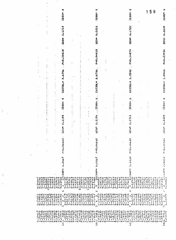
~ Q Q

1 5 9 0

... II II u cr cr cr a: a: a: cr cr lol lol lol 11.1 - ... co co ~ .. ISO - - (\1 '"' (\1 "'

,._ "' - -. . . .

c:o Q c:o 0

•· • " II z z z z lol lol ""' 11.1 0 0 0 0

CD <D .. ~ - - .... .., oD .0 <D a-~ • ~ M Q c:o "' . . . . Cl 0 0 0 If; II II II ll. ll. ll. ll.

4 oD "' .n Cl' Cl' Cl' .. ,._ .... Ill ..0

"' "' ,., a:l

• . . . 9 Cl ~ ....

"' • II' II .J .J .J .J (I (I (I c Ill Ill Ill Vl - - ... -X J: ::: ::: u u u u

0 ~ 0 0

II• "' If ll cr cr a:: .X a: :z: a: a: lol ""'

11.1 :.u ..... -~ ~ - ,. "" "" - ."J - ..... <:tl ~ .... • . . .

C! 0 0 0

g. "' II II <: :z: z: ..,. .....

""' .oJ .oJ

0 0 ::J .J

C\1 (\1 0 1' 4 .IJ . .., :\J -<f <41 ~ ~

-41 4 .. .? 0 0 'J . . . 0 0 CJ 0 II II II •I :1. :\1 .:.. .l.

.... .... .., ':J .c. .::) .., -" 4 .., ..,

~

"' .. ..., "' . .

-:> "' :\J

lt. "· II II Q. :l. Q. :!. a c 3 :" Ill "' .ll "~ .... -

-~-~~-..,~~o~o~~n-~-•n~~~.~~c=r=o~~o~-..,o~~..,-=~=c~N..,,~~-~=~-.~~=­.n,_.o t::N:..C ~.z;-~ ~,JlU,~,...o-ru.---..:.-'-,J\4","\J..OUC:'>-,~-("t')"'-."l,\J.IJ:.r. 4>~'-l,...._.;._) 7', ... , _ _,_a .. ~...t j>- ..r.::; ..,....,~ ·.;- _.l \.i .:O....,.=»,.._D-.Jl~~..C.!J T -\I . ...,.C.-. . ..,- .. flJ'I 'J\·..,.,""""'•'\tr :J\ ..n-.::~"~.J..::-:o--.J~.C..._./' __ \J f) ...,.,J"'O:>."._.t'1..C1 -.n ~= .:- .:0 ..;::!ll.'\J~~J'..IJ4';f\:\.I./F.., .._..C3t::;,..,.,..,,._J:3'o.'\tr-~4")~~ .C:J'lO~!J·~i)."\/.fl..0-"'-.\1.-,.ot -.:J..l;..:-G-,..-~..,..:..-.;;•,1.} =: """'Ot:J-4Q.t).:$>_.,iJJt'"::i.O rJ.:I'-.O:Tll~.'\a:J:J'I t)..._..,j-:t;~- .OJl..._..:t'.Ci"'rJ."\J.~;"\,j../";'Q·l":J't'- 4'- :::!'!..::·,'\!.!:':r.::Jr'.l'.J1r. O'"J -..'"'1

• • • • • • • • • • • •. -., • • • • • • • • • • • • • • •M • • • • • • • • • • • • • • e.;f' • • • • • • • • • • • • • • • ""' • on~-.JJ~-~~~Nn n-~~-,.,-~..,---~~r ~o~~~~..,n-o~-..,~~ o~r~•-~~c-~w-•~ c

-~~e~.cN,...oo~•- ~~M~~~~n~~ .... ~-~' ~~ ..... ~~~~,...~~~-~n ~-cc~c-?ec~c~-~ ~ ___ ,.... .,.~ _,.,_..o ... .., £ =' ~"\J 1"':1"-"JN"O,.,~!"'--·- "~"'.c-.-,~ n :·:>=> o D ..... '-......, ..... 3'"' ;o 'l'·'"1-t- ~.:: ""4' r.~ )\ \J·r; 1- 1" .-.; !"- "'1,..• o~~~~M~N=~~- ~~-~£~e~DE~~=..,~ ~··-~-~~~--~~~= ~:~~~:--:~~cc~- ~ _r..x;. ~ -1-~..n.;; ~ .::~·r--1\ .x--.f'! n..c .n-r --"\./:\.; ::>::n .. \J .;; ::~-...c.-or: 1'-~--'i -T \Jr . .t- \J..: ~ .'\J-::.-. ~ .. !'", '\,i:..-; '~·.._ .:--- "" ---•n~•n~ncn~~D-~~M-~~--..,=~-·---~~~~=-~~nr~=•~-~~~~n~r~~~~~~~n . . . . . . . . . . . . . . . . . . . . . . . . . . . . . . . . . . . . . . . . . . . ..... -........ . ~ooo~n=N=-~~ ==~ooooN-ooocoo ~===o-o-ooo~ooo c~=~==--~==;=-~

~ ..., N r

r--,t:J..:t~-4""3":X:M~C"'Cf\.J.-:J: ~t\.'::NMO"r-o...c:r~-l:!,.._.:!""""C-.;:-t,'\J..t: f', .,.~?'M..:J-:""'-OCI'\J!'':t'._:'-:""'--./'I.;T=o l". .l:i..:t~C -:-­-~-N~=·~=~~ru~·~~~·~NCO,._~-~~~-~~-~-G%~~=~~~~-~~L~-aJ·-~~~-c-~-~ rN~-~N~~n=•c~-~·~~~~~-n~~~r=~~-~~~oc~-·~c=-Nez7~~-~~~r~-=7c~-~~ ~~~-~~~~•-r~~=N-~-nc~:rc7•~c~,~~·~·~-r~~~x-~~-=~NNC~7z-~~r-~~n ~..__. __ :#'...,"-JC . ..,.'f't"'"'- 1'1--~C"""'!·J"I"\.:'.G-,_,·~:"'j..._;., ..:;-t'\.: ..... ~~~!1~"t.l:t..,"'..:..r~ --::-~c-_,..t- ..... ~---"\.!- .0.::

············-·············••....;••••···········~·············••.....i• :-ccc~ccco..-::C\.t__,-coc-o-c,...,c:.c.:-.-=:o~----'olo.;:ro-c-cN-e-•.,..~o_c_~~-..-::ccc.::.coo-c_-

~ ~ ~ ~ ~ ~ ~ ~

::0 ::0 ::0

0 • • • 1 6 0:: 0:: 0:: 0:: 0:: 0:: w w w -C\o N • N N • .... .... • - • . • co co • • u • II z z z .... w w 0 0 0

• .. • .... .... • CID CID • • • • .... • . • • 0 0 • • If If 11. 11. 11.

N N • C1< C1< • LJ'I LJ'I • M .., • . . • - - • ' • • II u

..J ..J ..J a a a Ill Ill Ill - - -:r :r :r u u u

co Q 0

II n II 0:: 0:: 3: a:. a:. .X w w w

' ~ 4'

' .... ..... :D i ,... I .... "' - 0 . .

0 0 e

II ~ II 2. z ·.u ·.u .u ::l ::l

0 Q ..... .., .... 0 ~

.,. 0 <T <T "" > . . 0 0 0 II II n 0.. .0.. 0..

.... .... .., ,.., .l) .., .., -<> .., .., -c -

II II II c.. a. :l. ;;, -;:, J Jl <Jl Jl _, _..

:\1'3'- => :l',;.-.-.:t ~~0 "\J.l::J :Ito"" I.·.., :0~-':"\1 ,.._~ ,:i.-fO•l' ..:1'--z:r- \JM.f'! .iJ ..0!) 1':::'"\JQ D ~ ..Qr"': = -.,.1":"\J-.:c ::0 ..,._..,c,:::, ..... l) ~-7' '!J ,....,:.() ..;i" .CNi.l) .Il3'- -:l-J<- .C._,.:.J.;J\ 3'-~ ~4' D<':l,-..:--...::r ~NMM"\\U..n."'\JJ'I!""'~·':l'C\.INr\i CO~ C =..;;J!..J....,~-"\.1 ::0 .:I" I"! ~'I,fYlX ·\J-: ...0 .:r-'¥'! :>J'\ D3"'"'\\r-- :=~D..,"'lC :t 4' J"'~ ~ ~ ~~ :~-.-.:.f"'.\J..O'\Jl)"C .Qo;..-,.-.;..., :1\JJ .n:'\.:--t""-:: -C"t;. -~ ·T- 1"-" .l' Ci .:::l"""! ....,..T '"\J X:...,....., .rs~ -:;:,u .Q.:) 4':'"'- .;:-·JJ~('I1'J1:'\J ~ .::..tl~·;\0-:a "'·""' "'lf.4" ~ :>4"."\J :::-.:Jr-.\.1 :\l..:r ~en n.:: 0':;) ..... \J ~ .::-r- 'r)~ .:r o ~ ~ .'1 .-. = !" ..... r"l .l)~==,~~~·...,~-~~ .D•-•~~Gn.D~..,oD-n Qn~~.D,._~~~C~<T..,~N ~n--c-n~~-~~~"N

• • • • • • • • • • • • • • "f> • • • • • • • • • • • • • • •N • • "' • • • • • • • • • • • •.;; • • • • • • • • • • • • • • • ~~D-o~-N~~~~~~ o..., __ ~...,<T,...-~~~on~ •~•~D-•n~G~-n-Q ~-~~o...,~~ • ..,~•~...,-

~-~M·<r•eC~,.._-~z --~X.C~c-,._~M:~oc N~N--r~f-7~0~NN CM~~-~=c~N~~~-~ cn~non<r~~~~~=~~D~~~~-Q-~~~·•~c~c=•c-~=-~~~cn~~=~~nn-n-=--nn~n~ ~~(\.Ot$"1:r;-=fY'I3r..::C~..r ""'"'- !'- "-M'.f""'1...,.1.CJ-'""' ,.C:"'-,.._C :0 ~ ...C :'\J.C..::l~\"1')."\,o .:;~~S..;t "- '::: :" ... ,_~ -~!\J~.f"C '""- r-----~-~~~·~~~~--r~CO n~~~~=~~~~~Q~DC -~-~~~-~~==~c~• ~--~~~~P=-~~-~­--~:;:):¥'),::a-~..-, .:t--.O..,.,~--r:-~-r."\J.:r.o.J;-... ~!\J~..J\-:;,.r1o ~-:t-·=.._""':.'1.:1'~"'-"~~-,...~ !l\..~~--'\J:'"IJ..fl...,""'": -"\J-:1--"'\j-- ~ . .. . . . . . . . . . . . . . . . . . . . . . . . . . . . . ............. . . ............. . o:~::::to-.:::.::>o:\J:::-o:)- ~ ..... ..::.,:,=-~--~==~o~o::t ~'\J ..... -.;:, . .::~o~,::,o:r.:...::."'.-·:.- "::>\....,~ ::>'\J.=:~""'!-0!'\:-':::o ~~

_, 4'

·l:~~.,C~N-,.....1:-I.C'=',.... ,;:;~CC :C:::::.I"",J"'CO'J:O .C~ ..... .J"'·..Ot"1C'~N..t'.JJJ'.O:..C~"'\!-CJ" C-t.,.. C..._~-3' 4' ,_.,c -=:"\:i"''4" 11\'\."f"""''C _,..~:~~~~Nc•~~·~z~·~cc.~~·~c~x~~~=~o~~=•~~~~~-N~~-c~~~~~=J::z~: ...... ..;;;:!\.: :J'"-.· C"i-,......:- :..o.;..:..~:r-.:: J"'.~~.,..:: ~-l:l,.._:""''r.c .r.~'l:.f"--~.1"\ .nc-,...,...c..r,.""":: :1"!"\.""'"'·r.a. .J" -4('\. .:tr--~~~f'1o=::!"'7 ~- ..:J'-..r D7~-•ru•-o~~~ro-~~~=~N•---~-~-~7~~~~~NN-r~~==z~c~-c~-~--~~~~-~=-­_,_"' ...... -'..C "\J-!:'J"j :=N.O 1- .--~ "\oJ' ..:::.n r-r:·nf't"'!;.\J_,_J"l_ "\,;.l"l--...C ..0-...,....nt"\.:e.'\,;""'":-.]' ,~.;..a-- L ·'f'·'J"< ""l'Z j"'"\.: _.- :':10:: .............. _; ............... _, .............. -~ .............. . ee-coc~-ccc-ec_eccc-oc~oooccNo_e~-o~oNNC~O--o-_~ocec-oecco--cc

~ ~ ~ ~ v u

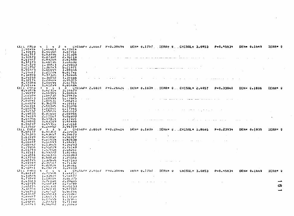
Ct.l L FRU~ .. 1 .. 2 .. LHl!>I.IP::o: i!.obbbT 1-'=0.38494 OEN= Ool1!:>( IERR=;:~ U CHISQLc Jo0853 P=Oo45634 DEN• Ool649 IERR• 0 1,•104'l4 lo'tt>'ttd b.(J'>Il<t 1 .:J•i41 5 Q,:"l4'+bf- J,tl/ft-.1 Oobl767 O,UJ~'Jb l.JJ.j20 0,3116'1'1 O,tl/Jt!O ~.3ol~d -- -··- ---·--0,4}<;'17 l),!l-lt.UH t..blb tl 0,311?3 0. 46}•-jf> l.hl:!tdtl 0.?.~,72'-l },HHlll Joi!.':iOtiJ I.c:J7q2 l.Jo'1<t1 !:>.21011 0.9lil?3 o.oo4~'> 1,1:14!>!>6 ? • 1 ')"1- ., t.tl?ll4 b,tH 1'+i: O,]I:I'H8 o.JtJ.:t, 1,5t:ou!J Oo<''>~l~O u. Jh0 1.J2 ~:~;11g ---··-· -··-o.J<'l74 J,c\14114 o. r~3f~t~ 1ollhlf'i4 J.ol7o~ ?. 11!444 0.412'7'1 b.b!:>4d4

Cttt. Fqf() l ,. ., l 3 CHl~UP= 2.0000 llo\Htli'h o.toi.'31 .. 3 .lllo l'J

f' = u • cb'H:Ut [Jt:N::a Ool8J'll IERR"' 0. CHISQL,• Zo4057 P•Oo33B40 DEN= Ool806 IERR= g 1, 'Ja4'l'l u.lfo<Ju<; 4,botl1J'+ I, t,u~ll'l j,O,.?JO !:>,cY47u 1 .t,ri2•· ':1 t • .:n<:>':I'J ~.itbll!> 2.H~I'\<Jl l,UlJ<tJl f. t>bi!.<•~ 1,htltl?9 o.Jt.l7A ... ulult o.~h314 t..h03d'> b. 3"'sJ4b o,or,0?9 l.O~'J~l C:.l7'i40 U,\6.,3? 1.'+"1?<:'~ J.~.;~}i.! 0,9'l0J3 0.014-+0 .:.oo'i4o o. 7'tii'lll (.',17167 ~.Ut:t199 0. 4 ~~'}'it> U,:>70u4 ,.ll'i,d 0,~110/iO O.•i.Hb9 0.4fJ'+'1b o.J62.H (),4'>)::,-> l.cJtbo 1. l c'~ll(' o • .; .. H~c 3.'74109

Cl:.t L Flll'll (' j j 5 r! et1l~L:P"' ~.oooo O,llol:H o.()JJt,o .:I,UY'.l!:>

~""'O.i:!o4c4 IJEN"' O.ltiJ'll IERH= U CHlSQL= 1.8645 P=Ool393it DEN~ Ool835 lERR"' 0

3,71)31'.3 (),4J~:J7 tlo3'ibl'i l.bJl44 0 o 4 '>0 '+II ~.!:itd11 0,})1.}04 0 .d 41!-t o.tlt.b3d 0,0(>407 {l,t>nf>'11 1.41>~01 2.0604?. u ,lJhut> 4o.J 1><:''13 0,(9'1'.>6 IJ, ':'>~<'I 4 2,70149 O,OI2'1'.i 1. !:JCE1 4t H .J,\JHi!.Ul 0 •. JI!) II 0. ~>';1;';>2 l.tH .. 66 1.4:$1114 O,IJtJJ/M J,lildbj O.J?-/'10 u.':>OllJO loC:''>~b(l O,H07~~ 1, J<:'O•t6 '+eciltU 0. 1J 1 o 4'1 r!. J<+"• 1 ., ~.tl13c 0. "., <l<l1 0 .liC:'O ;•4 1 o .H,I)(i<. o. ·~o~<--. 1 (1,/<J('J<J J. <:'II HtU

ttll f!-l~ij 4 . ... .. I Ct1i.St.i>o= (',66t>/ r. (I • I) 11}41) u. II<,.,~; l , 't ~<'I I

P=o.J~4'i4 llt:~l; o.l-t':Jf lfRI<= u LHISQLc: 3,0853 P;Oo'+5634 OEN• Ool649 lERR'" II

llo.]!li?l\ J,':IJ41.0 ... ~ .. ~71 CJ,n049 1 • 1 tl) 1 4 j.Ul..J,~~ 0,41,..fd 0, l C.l a fl c,J•Jou::, -0.·~111\S 0 • ut.•f-:jtJ ,:.~:,flw

0) J. t1f't'l ,, <', ::>i;.L,J tJ,u~1JJ :i,J,..·no lo'+i'J H '1, ':>//till -ft.~)b-1':--'J ~=. 'lt'•·,u? ~.ljv{Ub O,tll:\37 U,'t'>iiJ] t..!.JlJJ'td o, ti-<'•t' 7 I, b•> I_, 1 ~ollt'J'J 0,.:,•1'-t'l~ (J. J { ,. 1;~ 1. -1~ ~t~u (J. v >i? ''·' ,J , t?. I.~ I ·..j U,fli~O O.l+~i/'4~ II, ~<t.-'r . .-' t:.. v:, IJ .. 'J

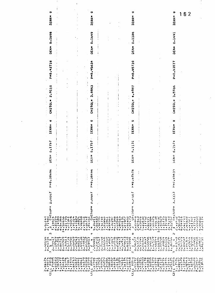
Ql 0 :> 0 1 6 2 " • n " IX IX IX IX IX IX IX IX IU IU IU IU .... - .... -(II a- .0 -CJ' • <II CJ'

"' "' • - - -• • . • 0 0 0 0

• H " H z z z z IU IU 1&.1 IU 0 0 0 0

:0 ... Cl ... - .., .., ,... .... .0 ... Ill N Ill Ill .., • • "' n . . 0 = 0 0 • • n II CL CL CL CL

Q .., ,... oC - :II a: Q - (II a- a-a- = • Ill . . . . N .., ... ..., II .. II II ..J ..J ..J ..J 0 0 0 C' tn tn tn fJ) - - .... -:1: :1: :1: :1: 1.> u u :..1

~ Q "" ::.

II • II II IX IX IX X IX c:. IX Q. IU ' w 1&1 1&1

,... ... - -? n n ..., ,... ... - _., - -. 0 0 e 0

II II II !I z .,. z. .oJ :.U ..u 'IJ :::. 0 0

... .. oC ... ~ ~ ... ""' <t ... oC ~ !X) <ll ... ~ ,..., ,.., D -t' . . 0 0 "' ~

II II K II ::. c. ... c.

..... ,... ..., "' ~ '"' ..... -<> -D ·' .., -D -D ,., . ;\1 "' ~

.., II II II II :l. 0.. ::. ~ ::;) 3 :! Jl Jl · • .f'l Jl ~ ~ - ~

=~=~n=~4n-.;;;~~~~-ru~=-..,~~~-~-~~n•~=..,~o..,o~~~•n=~~~~~~~~..,4~N---~~~ ~ :OU.""\.it\J.:ti::O .P:J't.: <-~NN.t\ -x::~..nu-."Q,"P\ ..- :/'.,~., .::- 3' 1: ,o.-f"")t.("·~:'\: J.; .:-.._...,.r,..."J".- ....,-, \J.-:: ::-.r;..;. ~ JJ.- :!'> "\.:.:...,-;- -~ _.,., -c­-~ ~~n"'lD-"l"'lN~=>~~-~ N•~-~=n~,..,nn-n?- =•n•-o,..,n~~n-~~n ~=~-Q~~n=N-,c ...... ;:)(\,tot 7.:.-~~'l--4-.D-..c .t' _."l.:l.O 'J"'l ..... ·-1" -:. ..... :o.c.~-.CJ~ ..:.~.n.., ...... \l:'\!.C""'l'\J~.o:::...r 'o.,l ..... ..;..:r '-'- _ .. _:-_'i=~ c._ -N~·..n.ttN~3":1'.7-.,~3't·:o...:. ;"'")..Q..n-'f'x:.\"'!l:"""l·...::.:>:X)JJ:.-.:t.n .\J.D'\J'\J....,~:l:I:.'J'.,:,..;t-_. ......... :\J t"..tl~~.t:J-1"~:-o:::o .. ,.,., ................. ~ ............... ...., ................ ~ .......... . DN ... ~~D•••~-nn"'l~N- nN~n--~~~~•n~=~ ~~~~-~n~-~---ry~ ~..,~~~~~~w~-

DD ~~-~~~~=~~-~~N- -o~~<=~~~=~-...,o• ~c~~~c~~7~x·~~~ =~~-r~~-~~­·---·~=-~-~~D•~~-~~~~~~~c~n•-~~~~-~1~,?~~~~~~-~--~nt~~~~~~~~--n ~~ ~~~~~~-r~~--xac =Lr•-~£~e-~a~-~ ~-~-z~-~~~-~-~- ~~~N~C~7~Z~ ;c_"'l .1-o.::>.:::::z.:;-~ .O..fi"::l~~-'l'J'l 7'fl j" -c ~.#'! ~"\J !."1'- ~::1' =-n ..c ..,.~....,~..,.,~..r ~ ... -:I''!"~-:: ....... },.:; '"":~- 7'- :1' ._,At..~!':-:- ...... ::; :t" L.Jl .................. o-'""l.n-.'\J"'\J c.:~,..,. J.:.t:."\J..n·..,_.l ...... ,o,...,~.,. ,.., "\J:'i ... '1..C =- - ... "1..,~1_.f"! .:::-.f'l n~ ..r o)-::. -,~ ..(J ~·.r.,:) 1'-.fi ~:::; 'J~ ·"J -:-r . ..,..c . . . ............. . ;= ~--o=-~~=N=-o~o ....

. . . . . . . . . . . . . . . . . . . . . . . . . . . . . . . ........... . ~~=~~~~~-~-===- ==~~==c-~~=~=;- =~~o--=~=-~

~ ~

~ .;~"Ctt";~M,._O'~I"'-"'Crw"',f'-.1--.,..:J'IoC:-#'-o.r."J' ..C~~X;J';c:..C 00:. :2..._..t\...oi~::CC!C'O"C.OJ"-...:: ..C-.:j-;,!",C -.:...._O'·'Y<"""'::""-OC ~ ... · 1'-.!: N-~~XM~-~.~~~~·~-~~~~~~~=-c-MN-~-~-~~-~~·r~~-c~-~~-~7~~·~~~-C~ .::-o::.cc.Jl'./":-4' ~-=3'-X!""-..C.:c...:c-•..,C\..:t.~"-::: ~ .:x. ~~t.Zo..:-~..c-·:..:r::;.-...:r:-a--~or-.,...o-f'\,;c .;r-~ r ...J"u-• .-..r.-,.... . .:;:7 I'\;~ •=~~=~Q~•~-z~c~=~~~-•~7r~~c-~~7•-=~~=~~~=D--c-=--r~-~4N~-~N~~~ X.._ ~O~N=~--4~=•-rN c~NaNNC~CNO~~~C ~~=n•c~c~~~Nr~~ -~·-N~~~~~-••...J•••••••••••••••-J•••••••••••••••~•••••••••••••••~••••••••••• No-==-•~c-occ~cecc_cc--=-o----N-c=-==-==-ru=~~=e=-c--=~-cco-c~-

~ ~ ~ ~ u ~ ~ u

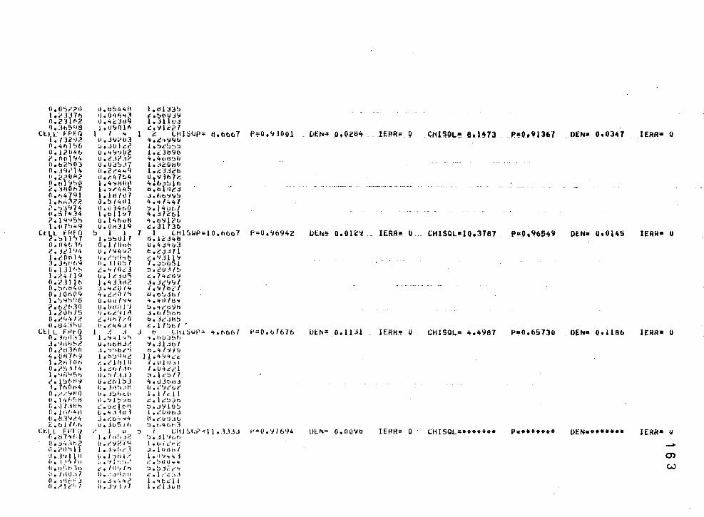
O,OSr'?tl I.;.on7t. O.;?Jlt-2 1t.:H.,b'rS

Ci:.LL' ~NQ I • 13'i'o.J2 0.4hl~b O.l?U4b r.noJ44 o.o2~03 0 •. :l'li'l4 "•C'20il2 Ootil'I':>O 2. :;sOt• 7 0.!'14791 },t;..;3?2 ·?. ~347 4 o.sr ... 34 ?.)'1'15':> l.o7'•49

Ct.LL FRf(l ? • ~II'> 7 0.04tdl) c.Jtl'~4 1.~0614 J.J'JI'/.9 U.\J}h':l 1.?.4114 o.CJII t; o. ':lr,o4 n O.JO<'>(l9 1.':>'1':>'18 ?.o2~>30 l.20kl5 0 • .- '• 4 7 ~ o.u~:;">o

Cl:.l L FRrQ 0. :ltJ i) 33 J.o.J,;B..,c o .?tnnn 4.UII7f>'} lo?.B1flh o.;>~H4 I , 'rll "0:,.., <' .l !;!6H~ l.7h0t>4 0 • r' ,• 'Ill<) t>. l'•h'>H 0 • olf .HI'> o.lf,t·4tl (). iJ :i'-1<'4 <:.bj/1.1-,

Ct.l l FFI ~~ t•.ti741d 11o::>4J~;2 I] t ;>I) 'I}}

''· J•;j Ill [I • 1 -~ f .. .., II

0 • II~-~ f) 1n (I. I riiJ i> 7 o.>•lnr.j 0 .II c'· ·r

l). tl544fl I) • ()1jf:>'+3 Oo'il::3d9 loll'JO)h

I t 4 (1 0 J':li:'IJ3 lioJUI<::i' 0, '+':I'JU2 Uo<'J?.1? u.OJ':>.17 0.2?.449

''•"'" 7!:>4 lo4')rHUtl I• '>r''• 4 b loi!HU7 o.:>t41ll o.v34~>0 l.ol b7 O.l46utl u.ur\319

!> I ). 1.~':>017 0,1/0t>ti u. /':14 '>2 (j. r'~J9i h (J • .l)l)~ 7 ~. ... 10<:3 lJ • I C. :IU'i 1.433!12 3.'+.:'01 .. 4 oleO I'; o.ovl':Jit u. (Jtjij l •j >J • ul: '4 I <i L.lih7,"'0 u.I44J~

1 ,: J I • '>" 1 ,, '"> Uo<>oHJ~ .i. "1,hl"~l I • t>'.>4'+ i:! ~:.clHIII J.t::r,(.i.-. u.:> t:uJ o.col~J (J • .li1~.1H l, • .J~hr.h tl. 'II ~·,6 c:.o~ltoH (J ... j]td J. t:t>'•-.4

.,u.3v5th " 1 lJ I , f rt ~~ J ;>

u. c':J?·r" 1. J·tf)~] li.l'l61? t. • I..J ! .... ),j

c • f II'> I h lJ, .-: ;;llo It I} • j 't 1~ '-4-? (). 3'J l '7

l,l:lD3~ io!>bUJ':I l.JlluJ c.'llc?T

l ~ LHJSUP~ 6o66b7 ... l•t':I41J i.~c::~-.~ i.c::.3b96 4o4otl':>!J I.J<::OtJII l.r.J.Ub u,'l'3t>7t: 4,td!..lo tloO 1 i)('j .:l.t>b\1':1~ 4,4/447 :..j4Ut.r· 4 • .:1126 4.o'>l2t> .:.31736

1 1 lHl5WP;lO.b6b7 li.li:"34b Uo4;,'+!J3 6,2JJ1l C.,YJil'-1 -I.J~i.ISI :>.2u3r:. c::.74£'0'i J.Jc'l'll I .':17b(.' f tJ.o!..Jt>l '+o41lfb'+ ~.'+ro':il'l J,LI~bl'l o.JrJH~ c.ll':Jr.t

J o Ull::ii>!P: 4obbbl '+,o(JJ~t. ':J,JJ.lbl n,41':JIIJ

1l.4':J .. ~i:: 7olllll..ll l.u4t('l ':l,l c::> 17 'I odJotu tJ. C:'J((Jt' 1 • I I r. I I c.. 1 C.':J '"' ':J.J':I!U~ I • c (HI td il, rvtl_,o ~.tl4oi:J

"> 7 CHJ~UP~llo1JJJ ~.j}~Jbh

l.o/c'I'C. J .l lldtl ( l,..IJ"'J'tit) ~~. ::- u u 't 't ~. ~ ,,i: ~~ .. C'. 1 (1 ~ :).i 1. 'ttC.: J 1 l.d Jl>i:l

f';:O,'JJOOl _ Df.:f\1~ .O.Q2t>'L _l.ERR;:_Q .. CHISQL-.a 8aU7J P~O,'Illl:!J

p;Q,'Jb942 !JlN." 0.01~'!! _ IER.R• Q ... CHISQL•l0o3787 p.,0.96549

P::O.o7676 UEN; Ooll·H IERka ~ CHJSQL= 4.4967 P=Oo65730

1'=0.';1'/6':14 Ul:.N"' O.OO'Ib IE~H= 0 - CHISQL=******* P==*******

.. !l~Na Oo0347

D~Na Qo0145

DEN., Ooll86

DEN=*******

IERR• Q

IERR• Q

IERR• II

!ERR• U -0)

w

::0 0

II II ~ ~ ~ ~ w w -• ::0

• -• N • ~

• . • Q

• • II z ·z w w 0 0

• ~

• • -o • ... • 0

• . • c n H

C1. C1.

• -o • CJ<

• ... • -o • . • Q

• II • ~ ~ 0 o·

"' en ... X X u u

0 0

II II ~ X a:. a:. UJ UJ

.... ~ ,., "' --.

0 0

II " z z ~ "" :I .::l

-c N ... -1:1 -'l -4" ,... ~ .Q :> . . ·:> 0

" II :l. .l..

.._ ,.._ ·~ l:' .: c .c. .c. . ~ ·;>

II II 0.. ~

':) ~ J' U'l ....

~,.._~.,~~~~n-~~~D•~:>CQ~,...~~ ..n .o.c:l' "~...; .""":\i~"' c-, .c ~..,. il"..::Ji"'"--~ .. =~ N,.._~~~• ~~"'~~n~~n~n~~~~ ~-c~~c •-~~~~a~arn~c~~ ~c~-,.._:. ,.._o~~-~-~~~--n~, ...... ':) .............. ·~ •~-,n~ ~~-~~N~-~-~~o-~

~-·~~n ,.._,.._,o~,..~•=nc~1•N ..... '"'l-:r-... -::\1:'91 n .c""""' :.;--.,.... .::1 ...... """'~.~ t--::." =~~~~:> =~==~n=r,.._=~•=-­n~a~r~ ~-c-~~n~~~o~~-~ cnr~=,...n•-~•~~-~··~-~·D~~ . . . . . . . ............. . ~-~=~~ o-=~~--=~oN-~~~

~ . ~~~~~•a,~.c.~~~=z~~~~z=~a -JL~~-~~~~~~~~~~M~~T~~~

-n--ru~z=~•J~-~=nn:~o~n~ -~:~rNN~•~n~-~-~~=~~~c-==~ •~•n-~ ~~~•-=,...~==-oocn ....... - ••••••••••••••• -J -cc-No~-=crocoo~c-ccc~-.... ...

u u

1 6 4

APPE'NDIX C

165

FUHTM~N !V b LlVfL il HlllN IIATE "' 77250 llt/1 0/43

oonl 0002 oooJ ono4 liOf•~ OQI)f> 01);)7 uonfl UOil~ li tl t I) 00 ll ou1r Oil!] OOH 11015 out~> 0017 UO It< 0014 oo:->tl uu;>l no2r 1)0,>3 u 0 .>4 l:t)?":> li02f> on;: r vn.?H Ut•29 u •.no 00 il uo l? v ll ~ J l•tU4

'"' i'• un~"' UIJ l I L U Jtl (If) j4 l•040 OG'+l UU4? 1.043-­(;044 OU'+~ 1ill4f> ll047 (H) 4 h Oil4lJ VO'>O \J\)1_:,) {J OL'Ji' on·, 'i dlh4 uiJ">S liO'll> lltl'> 7 u l' .,,,

Olt~~-N!:dUN lNllllll tbi~U(10) [I,TlHol< bl<

liU flt.AI.d~tl01 tEfji):::50) U~ oltbNU IU~ ::Uf+ • J wt-< I H_ Ill t lu.C I lll', f t I MNO I 1 I • 1::: lo I OF I

. I i =lUI' + l r.r.~tiF/i::•••1 Lt;;;(J lltMS==!Of+!)~f+ol A.:.S I l•flt b lli •W lt lllOUilld·•t'••lU.ll ASSIGN 1 fO U~ I)(J ~0 J=J •'•0 I.Jl) 1 () 1 "'1 t 11

1 u 1 i~ i I I I"' il [,() ') 1:ldffo1~ v==o UU >! 1\=:l '"~ y ll.~f'"flt.l\t' (l)j wtdli (totJ<J<,)YTtMP

~ Y=Y+'r IUW 104 fU1~1·11d (t tffo1Po:fol-bo'+)

!JU IU bl1• (oo f) 0 yo:yq

Gl• 'I o ~ ., L=HNLk(lJ)

"idH lt•tlll~ll lO!J ~lJke~dfi' L"''•Ftio4)

~o:·r·r•L".! ~ WI< 1f ~-II, tl U :q Y

103 ~UI<MAf(l t= 1 •F'U 0 4) :Ju-+ 1'\-'ltll•F lrtY.ul.!JHJ(t<ll bU TU 4 I•• I I K l :: I ~. l I ~ l + bll f(J I.; '

4 cur,TJ•·•••r I I• I I I 1 1 "'! r, I i I I l + 1

'' CiJu l I Nlit. CdJ:,ut'::.v Cr·oJ ~'''-"'" llU !~> l=ltll It I 1 r d il l • ••I • 0 I 1> 0 T 0 i <t 't "1 bU 1\.1 j :,

I" Clll:,•;L::.Ctll:;,()l.+l~lf(Jl"PlOull'•TIIl/tl I ~J Lll J ~I; i-' :: L 1 il ::. (J I• + (( Jr., ) II ) -l ) if "i' ) It'

H ltl l ~ '' oi •I o1 1 1/ Utl~t,L:''"''

i-'L=<;·., Ill.:;..,,,., { l.'( Hl ;:;:lJ··~tJ

It -'U i>U )U j-1

}h Ci11~l!l_.: . .~.,itJ.>•'!L+\:h!~:l·.;L •>•LL (t;IH\1 H<;.oL.thtl-') tl;l tlh'Hl)

l'l <>.U l.t.I;-:IL•il<;IIJ't<H oi'Pt•H·,JIJ.ii-<) ""'' IL (,;,I'·" l Lrtl '>•>r>,t'P ,I!:' • lti'P,(:rlj ~IJL•I'l. ,nt_, lt.RRI., ( INT ll It I;:Jo I I) .,:,I I I (,,, Ill!• l l,H ['>!,~·of' I-· old·, I tf,,,,Uil ~I,L ti-'L,Illt H.llHI_, Ill~! ( 1), 1::1, t J)

?:.1 ~. U1, ( j 1\JI"I

PAGE 0001

-0>

0>

fu~T~~N IV b LE~tl ~I l'tAIN LJA TE = 17 250 lit/10/43 tJO~q UOt>O u06l UOf,?

lJ(}l't3 00h4

Ullt>!:l

l;U 10 6U c,o El•ll t a 1:. t.

., l ,,p IUD fUHMATC 1 CHISQ~= 1 tf7oltt' P='tf7o5t I

f• lJLI'"'•H-..4t' JI:.Rflo:t,1J, 1 ~tiiSYL='tf7o4t 1 po:t,F7,~t 1 OEN"''tf6 ~.4,1 ll:.kK;Itllt' CI:.LL fHtAit}013) ~

lUI FU"MAfl~fJ.OtlOf7.4) 102 1-uf<~tld«' lltbHftS Of tHttUOtl": 1 tf3oOtltl EXPECIEU fHF.:w:ot,t-JoOtlt

I' ~>Odl<ltMH VAil!fS::•t10fdo4) -t:.NtJ

PAGE 0002

-0)

'.J

U~GHE~S OF FH~tUOM= 1. [APlCTED tHEw~ Jo tjl)IJf<IJAHV VALlJt-.::>: .i.lO'IU ... c:,~u <;.ttnu 6o3'+60 tloO'IcO 'lol)370 llo3390 VltM'~ Oo6"-H1 Vlf"''f'= }.7700 VHNP= I .t-433 l:::. -O.Oi'?l y; f.)b3'1 VTI:.i-11-'-" l • .JIJ/3 YTf11P= 1.0643 Vli'Ml-'" 0.76-+" l= 1.?;;>5"J

·V= 7.434/ Yl~H•'= O.i'')/3 'I'Ht-11'= O.J'Unl YT~H": \lob!:>~"' l: u.I3U4 y.- ~..~'J'•b )JfMP= Oo4(1bt> YHt·tfJ:::. (I • ..;Tt1'J Yffhf'" l.l6Jtl l= (} .O,t-':>'1 Y = <t. hI ~;., Yltril'"' O.'i!•~>t> 'I' Tf t·fJ; () • ,., l ':i V I L I II' ::; n • ~· i I I l= -l.'JHI Y =: do:~;> l'li Yltt1f'::; tlo':ililt':l Ylfi1r>'~ 0 •. 1t'Oto f I ( o·l P ~ .1 o I !> 2 i' I= u;tn:ll v~· , u .t.9,.,.,. Ylf•W" 1),44':>0 y 1 t I'II-I"' f) • (j I) .ll Y IF~•~>" o.•.o f3 I'= l .'ll'<c y; l).,PO .H> YlrNP"- n.I••:•'> Ylt:~:"'" o.··uu.J Y I~ ~'f'" I, ?!it,, I."' -tl • Ul' :1"> y: 4 • (HH)J

YlFr·lf'" O.l/1'~ v r t' ~"'"' o • 1 ~"- u '• Y It !••I'= 0 •. <11'>4 l= -I ,t<lltLi y: ':>.6tiH:l 'I' lf· ,., f': l • '' ~ n tt YIIH·,,_, ].~'Ul

YT~hf•.: O.l'fu~• L=: -o, Ot•"i I v~ r.J3<;e Ylft,p,;: O,;(d'J Y J t i~l ~l: 0 • '1 j I:, (,

Y II hf-'"' 0 • ~· '• I .1 l:. - l. t'~· l 'i y "- :. (If,'(/

¥ II- r .t' 1 • "lt. i y r ~ tw o. 1 · • _, (: v r • ,..,p u. 't 1'""' '

-0)

co

I.= -;l • 1:- (O'J y:o '+, 44t) I YH.M•;:: J,b-,t•C: ,.llr11'• I. 09ic'>' nH·•f-= o •. n,·~ l= -~;,31?1 'r = t>. ?.,''+ •; YHi·ol-'= lodf'tll Yl r~,l-'= 1 .o I r.t• Yf~l·!l-'= t),'Jlcj l= J,I;H':>ti y:: '1,113<.U 'rTtr·or'= 4.1!\t>tl YlfHI•= o.~clc r TH•,jJ::: 1 •. ,..,:n /"' 1.~>4lo y;; l4.449't l'HHI-'= 0, 1Hi'>t>

n ''''"'" o .1 ?'th )Tf,••t>= O.A.u-. L=- -l,h«l.: Y= !:>,:lh/-IH YHHP= O,O]t,c: YHI•I'= '<olOLlj "'~~.P= n.urd'+ c= o.~~.,y y:;; H, (Utili Y I U4 P = 0 • I J 0 .1 tl ) T F 1-. P = <• • 1 •• u c Ylhof'= 1.".>1•11 L= -u.ll~i3 Y= ..,,44cl ilf~•P= (J,H9•,~ \' ftr-.P= (J,]4U':i Yltt·ol'" ll,h?.!i!< i=- -u.">""~· '(• 4. (Jl'it> ¥ I t o·W: I • 4 4 f b YTI'I·if'"' 1. fil':i I Y II· ,.,p = o • "> 4 J f t.o. -O,"ibl'> p.. {,1.11 11 ilft-,p: tJ.??<+H Ylf~:f.'= O,t<L;Jt: Y It H'= 0, c 1 cu l= J,?lr'l y c:: ". 14 I r· Yi~Hf'.: O.llii 1J'+ YliHI-':: 0, !lt:!"J YHNf'= O,fltlll L = ·- 1 • 4 I~ I~ y;. .-..14~~~~ Y It r··p.::: l, •lil'> I '( I' II f· = (, • '; H I b Ylti:P;:: l.Oic'J L"'- u. ?'•t. 1•

Y = l 0 • II WI 't YH I·•P= 0 .h'1/ J y If ~· p" 0 • :w I) J ilf.r.;p.~ ? •. ;•,,::. l= -I.J'<I~ y:. y, I h;> I

-0)

<.0

•)

·,:,

CIIIS!J "' hof-'-<IJ( P:;O.~:d:>td llt.r.:::UolOH'; II:.HR:::U l.niSQL= bo'-.10'+4 P"'0e5bll0 llt:N=Uel05'i IEHP=O CELL fHEQ YHt-•f' o.b~J~ Yll~.p o.::4o3 Ylfr1P O.}H::,~ /. = - 1 • 3 fi()ll y::; 4ehf>lc YHI'•P= OoUOtH> YH~<•f'= 0.7'>'13 Ylli"'f'"' 0. I I •; I /.= -1.4til' Y= 4.U~Oh YltMP= O.'loJb Y l U·ll':: C1 • ..._, I t• ,1 YlH·•f': !loJ':>t,'• l= -1.3?1'>'1 Y= t>.3~i74 Y T ~ l·i ~, = I • <; ;1 t> I YTi:l·lf'= 0.09H~ YlfNf'::: lloC'4t>:> L= u .h(Jh-J y::: ". Sll7ll Y H 111' = 0 • .: I f '+ YlfNP= loci {ll Ylf,·W= J,(lf14!l /.= l.fot\ld y: 1.7"'""' YHMP"' l.lf't1( '11-:t·ll ... = o. nuu Ylft·f'= J.ISt>l r::: U .f,H'it< l= lu.~'iHT Y l f ~.p" 0 , :< 1 i1 G Y"l~"if': (lo

1>14l YHhl-'= o.r.~41 L"' },Uif'l y:.. J,<'•d <; YltHt'"· i),{•;ll Y TFtoP:; n. ':.•'>c<J Ylf f"of';: 0 o'12t:'lo '"' .-',:H1•J y::: IO,Olil.! Yl~ltP: J,j>l!J(J Yl~l1i'= 0,9',">S Y I H'-1-'= ll,ll,'o4 ,::.. -II • '!( •,j y: h,41of<• Y l r t·t I' " !1 • " II J Y 1 t' ~·P :o H • 1: I 1 4 Yltt•f': '•,J'->01 l = -1 •. n J·· '; :. 1 '} • "',~,? .•. YHH'"' o,·,'l/'1 ,.1.~ .. ·= ).'•li") YH i>il-'= 0.41>6'< t.=- -v. ··11" Y '-' ;, , 9fl ;.>I Y lt· •·;t.J.: 11o .1 7ro I 'f f ~ !11'--" 0, 'I i II') YHI'i'"' ).1.((); l.:.. -ll. (,'--;~!, y::: ,.., • "_!]IS I y;,.,,lp.;.. f.,.h?~) ...

z 6 It 4 3 3

-'.J 0

Y It rtf'= I • 4 4 f f 'IIHIP= 1.32~2 t= 0,76711 ~= J·~.37H'J YHNt'= 0.~61<' lHNI'= l,!:l!lc'•t Ylfm'= O,i1S1t1 l= -u ,lih!:l.1 'r= 4,'1'111! Y T f t>l' = 0 • l :hi o YIHtf'= o.:tft>l y 'If l·lt'"' j. '2 j u '+ Z= -1.321'\t. y; 'l,'t'itd YlfNf'.: 1.,'<t!:lo YHt~P= t',71b4 YHt'f'= 0.314J l= l.t'i"3c Y• J4,lH6t> \'Tii·tl'= (i,h':IU'i Ylt, .... ,,= o.t:4~.lu

YH i'tt'= 1 .t>'J4l l: O.dftOb y:: t •• 037ti Yft;1P:: O,!:JQ()( Ylf.r,,...= I o'.llilt• YI~Mt>= 0,3)~'.) £; -2. (•tt4(: 'I = 1 :1 • '14 ·r t> 'r li-MP.: I. '?bJ YfFn!'-' o.rlo'> YHIH'= O,fl·no L= -u,t.24b yo: :>.(lf-.Ht Ylthl'"' l),O.,'t()!:J Y 1 f •··1•'" I. til t•J Y r h~ ,, = o • u r o 1 l= J,4f'4'~ y,. '>.4'f7 .. 'I'Ht·•P= lo'•h..:J Y IF~,,,= 0. '• r• ~ tt YH~•I'= l,f't•·i!:l l::. ii, 1HHI p: I. c'':l.ll Ylt H': loB4t,c' Ylff'tl'= l,t>f\ll':l Y H111->= O.t•':l2tJ z,._ _,,,, ... 71 y: '-1.?~ .. ]'-7 Y I F 1·11' = I • ,, f 1111 YI~11P= lo'•'i<'4 Yll-.1~1'" ?.:•h<ttJ I."- ,, • 144 j Y= lloi'ft>ll Ylft·1i·~ Uoltltft, 'r I F t·lf' = I • I '• I •, YHt,P= O.O'>itl L= -o.<tfl'i.t y; ? • t·., <; ,, LI1L>•JP" '1 • .'iJ.d 1'-=0,/ f'J't() l!l.t·t~U,uA .. (, Y T t ,. t, ~ n • 1 !-J ~) J Y If r:''" l. t, ., l V

-'-J -

ifl<fi"-IJ Clll"lOl "~""*""" f'"•><>ttili>!ttt UtN"'""*""n ltHR=n ClLL fHEQ 2 5 j ~ 0 b 3

YHt-,p:: o.T'hll I= -u.l7J~> Y= 'l.le>2f Yl I ~rP:: 0, r I !4 Yl thP= ).i'~t'Y Ylf~IP= 0 •. /d.j£' /.'" -0,64)U y: 4.<JOOb Ylt~.p:: lo'.>lcU vltr~l'= o.njlf YHI":P= ), OJ':IU r= -o,65Tt> Y= 6.111011 'HM-'= ).ht>U.J Yf!IIP= 0.44(13 YIH•f'= 3.JJ2o 1.'" J,i'41H Y= 12,4,-'>11 YltM'= O,C.St>/ Y1H·1f';: O·'•t;d! Ylrhf':: loiJH(Il z:: -u,..,c,or; v= 4,0J4l rThu>:: o.cr.t>c YlFitP= o,;>h(') YTH·IP= o.c~lO L= o.~!7~4'+ y; },7':ol'J Yl~hf'.: J, ·J.'-t;~ YIFtW= J.IJr''J'l Y It"'~-'"' 1. 'j':i'i'l z: ol,l~4/ ·r= I?,H4hf' YH_hf': 2.C''IJJ YlFt'f'= o.;ri-/1 YTfi·JP'-' 3.t'4UJ [;; -l.'H?i' l* l<o,77"lY Ylt ~,p:: l:'oOIIIJc '(lf.tf>= 0.773t> t I£ •·tP:: 1 • r. 1 "" Zoo 11,1141 'J '(: H.li'JI i·TnoP= Cl.4 fl:'O Ylt~•P'= 't•141/ r r F:-tf-1= n. 2'J3J L~ 11,0131 y-.. '-~• 7Y~~ Yfh·1P= 2 ... 11'-:1<' Yll~tp; 1,111•(() '(It I If':: 2 • iu';/ L"' -ll.I:J'•'+ Y =- I 2 , f' >J1.1 r 1 f 1·11'.:: o. 4 r u o YHI~P= 11.~-\':J':l YT~f.ll'= 0.4-lt.!! L"' -u.1l'JJ '(; J. 4 :17 ( YffM'= G.t;f.4) Tl t- ~!Po: (). 1 11<>4 YlrHI':: 1•-'"•/J l= (). (! 1>9.i

-....... N

Y"' '+ 6S<:~•.• Yltl·l~· ~.tdc~ 'ill liP O,tl'•~J YHH• ? •'><+ 1i l= U,1'lf3r' 'I'"' lll,">'IO.:I YHMP= lecd~ Y H.l·h;= 0 •<+•16~ Y I~ f'>P:: 0 • ll I .:It> l"' -O,':>lll4 v= 3,t:.'f4 r YlfrH•:: :i. l .JJ·I Y ll vd·'= n. 2rd'i YHr••f>:: ?.1/b'l l= -u .I 110t. v= l?.Jfl••'• YlfM•: 0,07~,(' Yffl·\!'"' loll'.>'i~ YTfMP• 0.42~u f.:< -0,3461 Y= J,24JJ YTI ~lf'= 0.'-1?40 vTF~tP:: o.·i<.J~.~ Y lUI"= I .'JcJ'J L= -o.~7ot Y= b,S''''"> 'f'l~NP" J,7illl1 Ylf:~IP.:: \.Jh.u Ylf~IP"' J,)">ltl l= -o,?'/?h y: 'J,lll'ld YTft-;1':: 2. o .... ~, Y H 1-lfJ: 0, ':l'HHJ YTFMJ;;: (),•Jf,1( L= -o. 3? 1 ,, y; 7,-l:if!·J YlFi~P= r.l'>b/ ) If ~11-'= I. '>'1U~ Y H t<•l'= 0. r • .-. ll'+ '"' -J.{l{''jt> Y'"- <;,11?3! y I~ I'll'= i:'. 4 I I u Yl ~ ~•I'= 0. ntll;u YH~,p:: j,.l'.I'Jh I= -1. Ill·(,;, Y"' lO,Il7J Yll-.1·11-'::: (;,h'IUIJ Ylfo"'l'" },:C,•t('c tHI"ofJ:-: O.l'>Hil t "- 0 • I '74'1 'r = 't. ':J''P.'t l'Ht"•P= (J,()(:Jc: YTf,••!-'= ll.l'Jbf YlH•oP.: O,JJ (':.. i:_:;; -1 • i'r(Jto Y = 4 • ~>t~O{~ Lit I "'J'''" IIi .OOill' Y T f ~'""' I!. I ,_'!>3 l'T.-hl'.: [),<tlill r r l '''""' n.; 1 G" L= --u. ·>I "r' Y; ] • { Ol ~ -.,

p ••;. tj 114 .:> t~LI~..;tJ • U~t> ., I t:fdl:::u l.lll SfJL::<><>~'"*** ~"'"'""""* Ul:.i~""'"H'** llcHR=* CELL FHEQ It

b <'

5 0 3 5

-""'-~

w 5

Yl ~ ;.;p:; 0 oiJI•'+.J Ylfl"W" O • .:I'>Mb YHi>IP= ?,c!IJ!> t.• -o.:i494 y: <:.,34!1il YTE"MI'"' ilo'+h!c YHI11'.: 1.4,'11 YHrw= O,l1~J l• o,t-?Oc Y= ::,,t>l~i~ y II. l·if' = (l • iJ 1 ~ , Ylh•of'= l.-1:-''t~ illiW= 3, ]?~1 /.'"- -11.574~ Y= 10.454<' Ylt-MP= O,I'IJ~ YH~lf':; I.O,-,u! Yfl:.MP:; 0.0'110 £;;. -0,610.1 y:; 3. (13/'J ~lF~oP: O,l-~!:14 YTH•P= il • .J~1>-d l' I fi·IP= 0 .I '+tJ':i z~ 1,304v Y= ?.9?1~> ~ lt~oP:: J, 4 30~ YHNP=" 0,7dt>.:l rllMP= lot•H.il l• 11,.,; ·r II Y= ll.~?ltl YH~1P= 2,23U~> Y I i" ~IP = 0. t-Ic: f Ylft-11'"' 0,23~'1 1.• _,,,ll~?b y" b.(} .,,)0 Yh~•P; o,\lC''JtJ YH~•P= 2,14tJ!J i'HMP= (J.3hcJ L• !,"!flo':) y::. 9.'•44r' ·n ""'= (J. O'J.Jt• YltNP• l.b•lt::; Ylt:r;p;; ~1.34hh

z .. -o.3""" )':: 10,??0.' YHt<,fJ:. 3.blo':J i'l~r•P= n.?oJ/ Ylf.NP" 0,'.1]11 L= U, O:iO'> Y= 'J.'iO/~ YH.,p: 0,144/ Y II Nl• = 1 , c 0 I h fl!CHf':: o.r'?.iJ L= -O.'•'J?J y;: j. -, ... -·~· Y I r M P -~ I • ,·" J '+ Ylf~lfJ'-' ';·.'-·•/:• I II I'll·'= "· ('r',-_'j

'"" 1,2]1J y:;:, ~~.(_.')fIt.,

YJI-!,f•c: ?.\·)'-J:> Y li·t:i•= I •''~'.II

-......, ~

YHI·II'" O.I>LH> lo: -0, I "lOt· y; 8,7011 YTfMI-'= 0,00':10 Ylh•tf'= 0.;2? 1:1 Yltrc,po= 2.lkc4 L:: -o,B4Jf v= ~.n?~<u YIHtf': O,J.,~o 'r It l•jp: 0 • .,:; .. ., v 1 r t ,,>::: o • 4 4 ,w l= l,lb1!. y; ~.lll,j\1 YH.Ni-'= O.O'!b::l l'IH•P• u.Ot;l4 v H ,.,.... o. ,,s..,~ L_:;; u •. , .... ,: y; ),tol'·\1 Y 1 r''f'" o. !>I· 1" YII11P"' o,~,4t:l

v H "'"" ·o • , .. , "-' , .. -o,o7n~, y:o (;',t>';{',:, YHIIP"' C.74<ttl Ylf~,p:: r,,:l<j~' Yll.•••t'" O,IJlt• L" -0 .~.f·b I y; <'.{4)0 Y lt ~~~·"' I. o,.,,,. lll hf'" 0 o <t'I<J•I YfthP:: UoY'Iit't /:= -\,(iltf<4

Y= "•"'dh 'r I r .-!I'::. tJ, <: .lu f )'Jh~f'': (l,':itl~.:;'

) a '"' = o • u • ·. ,, ·, i::. ! • f.'"> l fl Y= '),l?.t I '~' r 1 ~'''" ;>. ~:>J~·, Ylf '·''"' 0 ,f,,l I j l II I •I':: I • fl I IJ '.:> l: 1),4074 v~ . LJ.?~)4n \'l~i··i'= (),1)}<1 Y i I t··,p:: 0, (I I <t::> YH:·.i'::. O,<t ~JJ L .- 11, ;, i4 ,) y;; l • ,; c ~: h \' T' ~:1•" i). ,, I (j t YTt·hP~ o •. ,.i~l-, ) It I·"'"' \. , ...... i.;;. U •? r) _'S I y" .l,ff1/ (. t 11 ~ ~; p:;:: 1 j • .J. ~) 'i tJ;.; (I • '-)~~~I' i Yl~·l·.,·= ·I~On-td Y J f 1·-t•.;; J • JL'7·• '( 1 i 1"1!·' = d I' .. '~~.~-' [-:. -·}.f'J! ()~)

'r': :~ " 1·J 4 (l .. l

'( r t I ;;J:;_ ,' • --~t}t)_}

Y I i . :! 1 :.. l ,.111 •'.t·

"( j ~ I 1 :-· ·_:- ·' • ,. t ·, l

L·l 1 .:;l1 • u?;-'U Ji.:hP=o L.;tlSOl ::iHti:roei*~t4) P=*u~~"..-*** LJt..N;.o..,-u.-o-tHt lfRR=~ ClLL fHlQ b 3 !;) 0 2 b

(. --....)

(}'I

)

L;;; 1 7','>n Y= tl 111~-J Y rf MP 0 • toh'ill 'r'lfhP O • .lll•d YlFtu-> O,IJ'>4~J l= -0,3113li y... <:.3t-.4J YH.t-•1'= J,4h'::>b 'r'llliP=: ?,!>047 'r'H.MP: 0,4"/-(<; z~ o. ?'>'I•! y::: iJ ,lJ!I 3'.1 YHIII'"' 2olc1<> Y1 F t·oP =: 1 , 4 c 21l Y I F I·W = II • 0 llJ I l= u.v~lt> Y= (,129::1 Y ft t-iP= il. tJtJUc Y1H1P" 0.;·74'-J Ylf MP= l •'=><2'-.l'i l= -o,<J1f14 y::: '::>. fl) 'J ~ YHr,p: fl,711'.1c 'r'Tft-IP= U.lJ.l'::> Y rr l-oP= rr.t:Lltd l= l,Ot'-4.l Y: I I .4f'7'J v Tt 1•''-' = 1 •• ns r Y J I , •. p: ft, t'> 7 .H lltf·'f'= 4.cht>'::> 1.= -o.:)r-4'..> Y= Jl:',tJt-.Sf Yll:;-.p=: l.lh/d Y H r·.l'"' n • r- l '3 J Y H IW= I. :n T J L= -o.lht./ y:: 1.4? 1tl:J YTH1P:: (1,?-~c'.J

Y Jf ,.,p" I • "J .b '1 !f-11': 0 •'-•'J.J't L• -ll.JI-111.1 'y::. it. f·44l+

YTt·l·lf': 1,·:1~>'.>':> YHI"•P= 1.07(•, Y H liP: ?. , ,, I 111 l = 0, to 'l 0 I Y= t I ,t->044 YHr1P:. floll•l! Ylf.m'"' u,:Jlt..l YliHPo:: O,!Jt..U L:: 1 ,lo ">I) 4 y; j,<'f'-11 YIJIH-'o: 4,Jflt' YHhP= j), )'I.J! ) If liP::: (l, ;: d4 :, L.: -o, ·/l;'lu y::: JO,I?O/ Yl~r.P= loilc'<•'' y Tt ,,,.: (),(lfl ,::, Yllr•P"- fl,(o4_jU L.= l•. i' 1 'fb v= t~.ro~H

--....J

"'

'rlfMP= 0,4·1~0 Yff:tw= 2.~'1cl<+ 'rHicPo: Oo!!I<UIJ l"- -o,7H41 Y= 1\, 1>~16 YlH1P= loit>Jo YH<·•f= },43'1:> Y If I·•P" 3, 4l.~b l= )o!'>9H Y= t_i, 110<+ l'Tt o·tP-= (I,H'JIJ YHr1P: nol·~~u 'HHP= 4.1<+1'+ l= 2,f'47(J y::o ~~.~2'>':> Ylfl11-'= O,IIOtlt 'r 1t Mf'-= (l,hf'-1'1 Yltt-.1 1= 0,7}11 1. = -o ,ll'•"l y,-, .. ,414'1 VlfMi>= O.J?~o 'rfH~I-'" l.t''>~r: YHr:P= O,OfJ'> L= -O,I'A4~ Y= 4,\l<tOo Ylt~lf'-: 3.1!7t.~ Y H. ~It'::: (I , '>" I J YTF.-IP= ? •. l'Jb!.> L= 0. H'(fd) Y= t•+.400n YTHoP= l.ollhl 'r If Nl-': I • 2 l '+ iJ Ylf'Hf':; Q,i:'l<t4 {-: J.t,l-<Ut> Y= II ,I? l'J 'tH I•P"' u •''tdu Y 1 r t-oP= o. 1 r,,h Ylf11P: O,h91t! l_: -c',tl.,4c' Y"- ll,:hi\U 'r I H·1P= }. ·i 'do Y H hi'-, 0 .l 1 tU )11-MP'-" lo't·)cJ L'-" -II. '+0.'.1 y:; !,374? Yl~I1P·~ 0.2 .. ~':1 Y H t'•P ~ 0. I 4 t J Y H f',fl= n. ':>'-IJo l= II. I O'll "(= t!,., Oti""~ CHI~>IW=il.-IHJ P=II,Hf.;,cl IJI.i;...:t:,cl-j'>ll Jti,H'-'i! LH{':,0L= '-lol>f/0 p=u,1'J2.H Llt:N=U,Obl4 lt.HR=O Ct:LL ~HE.Q J 3 2 Y 1 t tH1 : 0 o (I'Hl J Y J F ;w:: 0 .I t ?.<: y 111-\P :; l • "u u" 1= J,0'-11)/ Y"- :;. , 41-< 'i•t Yrt~ot-'= (l,I!.->/·J YHt-.1'::: u.:'.ll<' Y I I tif':: 0 • I I J 1 L= O,H}7h y = ' 'I"''' YTI r-p;' ti. I l,'h

J 3 li --....J ""'J

APPENDIX D

178

H A S P S Y ~ T E M L 0 G

$ 20.37.52 JOb 711 -- HAI~AUA~ -- HEGINNINO EXEL- PAHT 10- CLASS 4 0 2U.3Q.J2 JOb 711 ILUOOll HAI~AOA9 ASM 23•~ REUt 230K USEOt 0010110~ ETt 00100106 CPUt 9,94~, 0000 CCOMPI o2o.J9.S~ JOb 711 ILUUOll RAI~AOA9 FOHT 230K REUt AOK USED, 0010014~ ETt 00100107 CPU, 18,23~, 0000 CCOMP 020.40.20 JOb 711 lLUOull HAl~ADA9 LkEO 230~ REUt 96K USED, 0010012~ ETt 00100101 CPUt 6.29$t 0000 (CUMPI 0 20.53.16 JOb 711 JLUOUll RAI~AOA9 GO 230K REUt 4AK USEOt 0011215~ ETt 00102131 CPUt 19,73$, 0000 CCOMPI *20.54.23 JOb 711 ILUOO}l HA19AUA9 SOHT 23oK HEOf ~30K USEOt 00101106 ETt 0010010 CPUt 5,19$, 0000 CCOMPI $*20.54.2~ JOb f1 -- HA ~AUA9 -- ENO EXlCVTIONI 140 LI FS

HASP3olol4 Juij STATISTICS-- 671 CARDS HEAD -- lt4lb LINES PRINTED -- 0 CARDS PUNCHED -- l6ob4 MINUTES CELAPSEO TIMEI

~

"'-J c.o

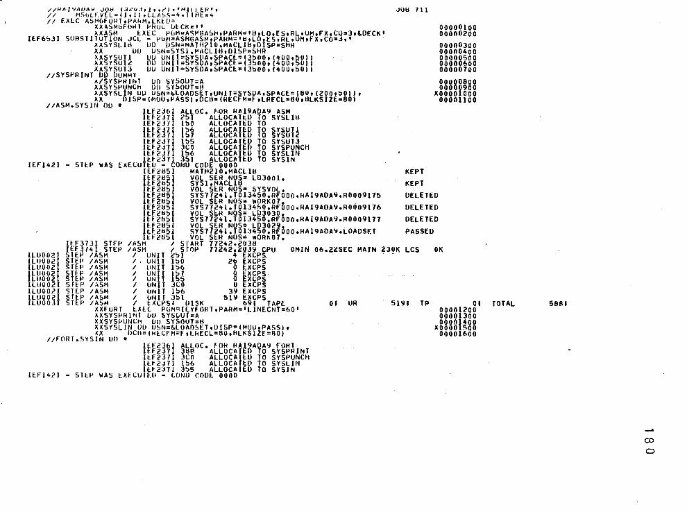
//RAJ<,~AlJAY JOI:J (3cVJolot2lt'MlLtfR't // ~15(}LLVEL=IJ.lloCLA~S=4d!ME='> II EXLC ASMGFURTtPAkM,LKlU=

KXASMGFUWl ~HOC ~tCK:II XXASM tXtC P~M~A~~GASMtPAAM=•H~lOtfStRLtUM 1 FXtC0:3t~OfCKI

llF6~31 SUHSTllUTION JCL- PuM=ASMGASMtPAHM='tielOetStRLeUMtfXtCO=J,t . KXSYSLld UD USN=MATH210,MACL1Ht01SP=SHH XX UO USN=SYSl.~ACL1Ht01SP=SHR XXSYSUTl UU UNfl=SYSUAtSPACl=l3~00el400t50)1 XXSYSUl~ VU UN l=SYSDAtSPACE=I3500tl400t5011 XXSYSUTJ UU UN11=SYSOAtSPACl=I3500tl400t5011

IISYSPRINT DO DUMMY A/SYSPHlNT UO SYSOUT:A XXSYSPUNCh DO SYSOUT=H XXSYSLIN UU USN=~LOADSETeUNIT=SYSOAtSPACE=IBOti200t~Oilt XX DISP=IMOUePASSitDCB=IRECFM=FtLRECL=80tBLKSlZE=80)

IIASM.SYSIN OU o llf23bl ALLOC. f~k HA19AOA~ ASM Itf£371 251 ALLOCATtO TO SYSLIB IH 2JIJ 150 ALLOCATt::o TO

l l~fJ71 ~~6 ALLOr.AfED fO SYSUTl lf~J7 57 ALLOCA lO 0 SYSUT2

ltf2J7l 155 ALLOCATED TO SYSUTJ IL~ljJJ 3CO ALLOCATED TO SYSPUNCH llf2J7l 156 ALLOCATLO TO SYSLIN ltf2J7I 351 ALLOCATED TO SYSIN

1Efl421 - STEP WAS EXE~UTtU - CONU CODE 0000 l£fc~51 MAT~210oMACLI~

l ~f2HSf VOL SER NOS: LD300lo E~lb~ SYSloMACLlH llF2H~l VOL SlR NOS= SYSVOL. ltf2H5f SYS7724l.T0134SO.RFOOOokAl9ADA9oR0009175

ftF2bS VOL SlR NOS= WORK07o Ef2b5l SYS772•l.TOl3450oRFOOOoHA19~0A~.R0009176 I£FlH~l VOL SlR NOS= L03030 0 ltf2H51 SYS7724l.TOl3450,RFOOOoRAl9ADA9oR0009177

l lf285{ VOL SER NOS= L03029 . . tf2H5l SYS7124loTOlJ450oRF~OOoHAl9ADA~•LOADSET

ltf2H51 VOL SER NOS= WOR~07 0

.JOI:I 111

00000100 00000200

00000300 00000400 00000500 00000600 00000700

00000800 00000900

X00001000 00001100

KEPT

KEPT

DELETED

DELETED

DELETED

PASSED

ILU0021 ILIJOO<?l ILU0021

IEF3731 STFP IASM I SfAHT 77242.203~ l£F314l STEP IASM I sroP 77242o20J9 CPU STEP IASM I UNIT 251 4 EXCPS.

OMIN 06.22SEC MAIN 23~K LCS OK

1Lll002f lll002

lll1U021 lLUOO?.I 1Lll002l ILU0031

STEP IASM I. UNIT 150 26 EXCPS SH.I' IASM I liNIT 156 0 EXCPS STEP IASM I UNIT l~' 0 EXCPS· STEP IASM I UN T 55 0 EX~PS srtP IASM I UNIT JCO 0 EXCPS STEP /ASM I UNIT 156 3~ EX~PS STEP IASM I UNIT 351 51~ EXCPS Slf:P IASM I I:J<~PSI IJISK 691 TAPE

XXFORT txtt PtiM=llYfORTtPARM='LlNECNT=601 XXSYSPRl~T UIJ SYSLUT=A XXSYSPUNCH OD SYSOUT:H XXSYSLIN UU USN=&LOAOSETtOlSP=IMOUtPASSit ~~ UCil=IHECFM=f•LkECL=60tHLKSlZE=IlOI

IIFORT.SYSIN UO o ltf2lbf ALLOCo FOH RA19AOA9 fOHl Itf2J7 38B ALLOCATED TO SYSPRINT ltf2371 JCO ALLOCATED TO SYSPUNCH llf2J71 156 ALLOCATED TO SYSLIN lt~2J7l 355 ALLOCATED TO SYSJN

ltfl421 - STEP WAS tXflUllO - LONU COOl 0000

Of UR 5191 TP 01 00001200 00001300 0000f400 xoooo 500 00001600

TOTAL 58AI

~

00

0

/ ll~~~~~ SY57l241.1U13450oRFUUOoHAl9ADAYoLOAOSfT PASSED ltf2~51 VOL S~H NUS= ~ORK07.

Jtfl731 SlfP /fOHT I START 77~42.203Y Hf3l4l STFP /fOHT I STOP 17~42.203'.1 CPII OMIN 07o72SEC MAIN t!OK LCS OK

lLU002l Sl~P /fORT I UNIT JUH 204 LX~PS 1LU0021 STEP /fURT I UNll JCO 0 EX~PS ILII0021 STI:.P /fORT I UN{ f l!>t> 117 EXCPS 1LU0021 STEP /FORT I UNIT J~S 130 lXCPS lLUOOJI STEP /~ORT I LXCPSI UISK 1171 TAPE Of UR 334J TP OJ TOTAL

XXLKEU EXLC PGM=li:.WLoPAHM=•XREftLEToLIST'•CON0=!4tLTtfORTl 00001700 XXSYSLIH ~U USN= 1 &YSl.FORTllA 1 oDISP=SHR 00001800 XX UU D~N=SSPLibtUISP=SHR 00001900 XXSYSLMOU UO USN=~GOSET!MAINltOISP=INEW,PASS)tUNIT=SYSDAt X00002000 XX SPAC£:(THKtl20t5olll 00002100 XXSYSPRINT UU SYSOUT=A 00002200 XXSYSUTl UU UNl1=5YS0At0lSP=I•oDELETEltSPACE=(CYL,(l•1ll 00002300 XXSYSLIN UD USN=~LOAOSEToOISP=!OLOtOELElElt) Xoogo2400 XX UCH=IRECFM:f,LRECL=60,~LKSIZ =&o 00 02500 XX 00 UUNAHE=SYSIN 00002600

Itf2Jbl ALLOC. FOR RAI9ADA9 LKEO llf237I 1~0 ALLOCATED TO SYSLIU ltf2J7l 2~1 ALLOCATED TO IEFZJ71 ~~~ ALLOCATED TO SYSLMOD llf2J71 3MA ALLOCATED TO SYSPRINT

fEF237l 1~7 ALLOCAJEO TO SYSUJl- 1 tf2J7I 1~6 ALLOCA ED TO SYSL N

IEF142I - STEP WAS EXElUTEO ~ CONU CODE 0000 llf2851 SYSlofORTLIB KEPT llfcU!>l VOL SEH NOS= SYSVOLo 1lf285l ~SPLlH KEPT llf2851 VOL SER NOS= L0300lo llF285l SYS77241.T013450.Rf000oRAI9ADA9oGOSET PASSED 1Et2U51 VOL SER NOS= ~ORK07 .. . _ llf2851 SYS77c4l.TOl3450.Rf~OOoRAl9ADA~oR0009l84 DELETED 1EF2851 VOL StR NOS: L03030o . 1EF28bl SYS77241.TOl3450,Rf000oRA19ADA~oLOADSET DELETED Ilf2Ubl VOL SEH NOS= ~ORK07.

IEF37JI STfP /LKlU I STANT 77242.2039 llf374l STEP /LKLU I STOP 7724?,2040 CPU OMlN Olo59SEC MAIN 9bK LCS OK

1LU0021 STEP ILKEU I UNIT )50 84 EXCPS· ILU0021 STEP /LKEU I UNIT 251 14 EXCPS 1LUU021 STEP /LKEU I UNIT 1!>6 27 EXCPS

fLIJ0021 STEP /LKEU I UNIT 3tlB 5 EXCPS LIIU021 SlfP /LKEIJ I UNIT 1!>1 18 E.XCPS

1LU002I STEP /LKEIJ I UNIT 1!>6 157 fXCPS . . . . _ lLUOOJI STEP /LKEU I EACPSI DISK JOOJ TAPE OJ UR 51 TP OJ TOTAL

XAGO EAfC PbM=O.LKEO.SYSLMODoCOND=II4tLTtfORTl,l4tLTtLKEOll 00002700 AXSYSIN UU UUNAHL=A&MJNPT 0000

22800

XXSYSPHJNl 00 SYSOUT=A ____ 0000 900 XXFT05FOU1 UU UONAME=fORTlNPT 00003000 X)(fJU6FOOl Ull SYSOUT:A 00003

3100

XXfT07FOOl Ull SYSnUT:B 0000 200 //(;0 FTOI:!~OUl 00 DSN=~f>TleUIHT=SYS0AtVOL=SEH=WORK05t 11 nfSP=INEWtPASS)t0Ch=ILRlCL=133tHECfM=fbtbLKSJZE=39901, II SPACf;(J~9Utl40tlll //GO.FORTINPT 00 ~

llf2J61 ALLOC, fOH HAl9AOA~ GO llfcJ7 l~h ALLUCAT D TO PG~;o.UU IEF2371 3HB ALLOCATED TO SY5PHINT 1Ef2371 3bh ALLOCATlD TO FTO~FOOl Ilf2J71 JEIC ALLOCATED fO FT06f00t IEtZJ7I lCO ALLOCATlD 0 FT07FOO

451J

3051

-co -

Ittc37I ?~0 ALLOCATtH TO FTOIHOOl H.f!42l - SHY wAS tXtLUTtU - CUNU COVE 0000

ltt2~~1 SYS7724l.TOl34SO.RfOOOoRAl9ADA~.GOSET ltf~U~l VOL 5tH NOS= WORK07. llt2U~l SYS7f24l.TOl3450oRFOOOoRA19A0A~oTl ltt2b~l VOL StR NOS= WORKO~o

/bu I STANT 77242.2040 ItF H Jl STEP II:.F3741 SlfP /1>0 I STOP 77242.20~3 Cl-'11 2HlN 33olOSEC MAIN

ILU002f STEP /GU Lll002 STEP /bU

ILU002I SllP /GO 1LU0021 ~TEP /GO

ILIJ002f Sfi:.P /00 LU002 S EP /GO

1LU003I ST~P /GO //52 EXEC SORTO

I liN IT 1 ~b 8 f.XCPS I UNIT .3~H tX(;PS I UNIT 3~6 3 tX~PS I UNIT ..idC 3 lXCPS I IJNll ..'1(,;0 0 tACPS I UN IT C: :.o 34 E.XtPS I lXCPSI UJSK 341 TAPE

XXSURT LXI:.(; PG~=SORTtREGlON=&OK XXSYSOliT lHl !>YSOUT:A XXSURTLIU Oil IJSNAME=SYSloSORTLlthDlSP=SHR

/tSORTW~Ol 00 DSN=f.,TI:.MPltUNIT=SYSOAtVOL=SER=WORK05t II UISP=INEWtOELETLitSPACt=ICYLtllll /ISORTWKOi UU OSN=,,TI:.MP2tUNll=SYS0AtVOL=SER=WORK05t II OISP=INI:.WtufLI:.TlltSPACE=ICYLtllll /ISORTWKOJ 00 OSN=~~TEMP3tUNIT=SYSOAtVOL=SER=WORK05t II OISP=CNEWtUELETEit!>I-'ACE=ICYLtllll /ISORTIN 00 DSN=f.li.lltlJISP= (OLDtllELt lEI //SORTOUT DO SY~OUT=AtUCU=HLK~IlE=l33 1/SYSJN Ill> It

II

llfl42l - STEP WAS

ltf23bl ALLOC. tOk kAI9ADA9 SORT Ilf2J71 3Hl ALLOCATED TO SYSOUT ll:.f2371 150 ALLOCATED TO SORTLIB 1Ef237t 250 ALLOCATED fO SDRfWKOl 1Ef237 250 ALLOCATlO 0 SOH WK02 1Ef2371 250 ALLOCATED TO SORTWKOJ

1Efc371 250 ALLOCATED TO SDRTIN Ef2371 362 ALLOCAfED fO SORJOUT

Itf2J71 J5Q ALLOCA EO 0 SYS N EXECUTI:.U - CONU CODE 0000

ll:.f?.U51 SYSloSORTll~

01 UR

S2

1Ef2ti51 VOL SER NOS= SYSVOL tf2d5 SYS7724l.TOl3450,RF6oo.RAl9AOA9oTEHPl

llf2U51 VOL SER NOS= WORK05. ltf2851 SYS7724l.TOl3450.Rf000oRAl9ADA9oTEMP2 llf2U5f VOL SER NOS= wORKOS. llfib5 SYS7f24l.TOl3450.RfUOOokA19ADA9,TEMP3 llf~~51 VOL SER NUS= WORKOS. ltf2b51 SYS7724l.TOl3450oRFOOOoRAl9ADA9oTl ltf2USI VOL SER NOS= WOPKOS.

PASSED

PASSED

4UK LCS OK

bl TP

KEPT

DELETED

DELETED

UELETE.O

DELETED

Of

oogooo1g 00 0002 00000030

Jff3731 STEP./50Hl I START 17242.2053 IEF3741 STEP /SORT I STOP 77242.2054 CPU OMIN 03o4~SEC MAIN 230K LCS OK

1LlJ0021 lll10021 IlltOo;U ILII0021 IUJ0021 llll002I IUJII021 ll1J002I ILIJUOJI

STEP /SUHl I UNIT JOI 10 lXCPS STEP /SORT I UNIT J50 0 EXCPS Sl~P t50RT I UNIT c50 24 EX~PS SllP /SORT I IJNIT 2~0 0 EXCPS STU> ISUfH I Ul'll T 2~0 0 EXCPS SftP /SORT I UNif 250 3b EXCPS Sill-' /SORI I UNI 362 ltOOO lXCPS STEP /SUHT I UNIT 35Q 2 EXCPS STE.P /SORT I EACP51 OISK bOI TAPt Of UR

1Ef2H5l SYS77~4l.T013450oRFOOO•RAl9ADA~oGOSET ltF~b5I VOL StR NOS= WORK07 0

ltOlcl TP Of - DELETED

TOTAL 40f

TOTAL lt0721

-(X)

N

u L<.< n ll c

(\J

!tl

1 8 3

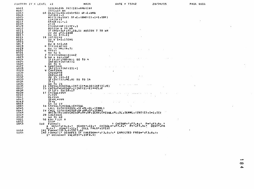
~URTUAN IV 6 LE~fL cl MAIN UATE = 77242 20/39/15

00()1 ooo<' 0003 000 1• 0005 OOOf) 001)7 oooA oon9 0010 0011 0012 0013 0014 0015 00 6 0017 0011! 0019 0020 0021 0022 0023 0024 002'=> 0026 00?.7 0028 0029 0030 0031 0032 0033 0034 0035 0036 0037 OO.HI 0039 0040 0041 004?. 0043 0044 0045 0046 0047 004fl 0049 00';)0 0051 005<! 00'53

U054 005'>

UlMtNSION 1NTI10lobNU(l0l lNll:.l>tH IJH

60 k~AU(~tlOltEND=50) Ufol:.obNU I uf =IJ~ + • 1 w H I TE ( 6 t 1 0 <' l OF • E.t HIND ( I l t 1::: 1 t I OF I I 1'-'Jllf + 1 KK=lJ~/2•••1 l~ =0 Jli:.MS•(Uf•ll*f+o1 IIS<;ltiN b Ill liR HIMOUilLJft2l.EQ.ll ASSIGN 1 TO bH uu 2o J=l dooo !JO 10 l=ltll

10 lNT<Il=O UU 'J l=lollEMS '1'=0 OU ll K=lti\K

ll Y=Y+Id:.XPIOl GU Tll llHolbo7l

6 Y=Y+Y GO TO 5

7 Y=Y+Y+HNOH<O)o*2 5 IJU 4 K=l, IIJF

H <Y.uT.HNU(I\)1 GO TO 4 IIH I K l "'1 NT I 10 + GO TO 9

4 CONTlNUI:. lNT(Jtl=INT(IJ)+l

9 CONTINUE CHISIJP=O CI11StJL=O uo 15 1"'1 d I IF<JNT(J).NE.OI GO TO H ZF = 1 GO TO 15 · .

14 CHISwL=CHISQL+INTlll*ALOG(lNTIII/EI 15 CHISIJP=LHISQP+CilNTill•E)•o2)1f

Jf(Lf l l!:so1Aol7 1·r CHISuL=999

PL=9<~ UL=-Y'J'J It.HHL=999 Zf=O uo To l'i

lH CHISIJL=CHISQL+CHIS~L tALL CUlHICHlSQLoDfoPLtDLtiERRLl

1~ CALL CUTHICHISQP,OftPPtDPtlERHI . . - -wH1Tt(8tlOOlCHISQP,PPoUPtl RRoCHISQLtPLoDLolERRLoCJNT<lltl•l•lll

20 CONTINUE GO TO oO

50 ENlJ FILE li SlOP

100 fORMAT( I CHISQP=tof7o4tl P•lof7o5t I A OtN=•oft>.4ol IEHR=Itllol CHISQL•••F7o4o' P=l•f7.~•' OEN='•f6 H,4o' lEHk•'•fl•' CELL FRtG'olOlJI -

101 tUkMAl 12F3,0o OF7.41 102 fORMAl(' UEGHFF.S OF fREEDOM=•oFJ.O,/ot EXPECTED FREQat,fJoOt/t

1' bOUNDAH'I' VALUES=•tlOFB.4)

PAGE. 0001

-co A

N 0 0 0

111 ... ' ~ ,., ' 0 (\J

z ... c I:

\j

<.:

"' "' -J

:.':>

>

;::: c tt ..... ~ 0 ...

1 8 5

~

....

.c •.!" 0 ~

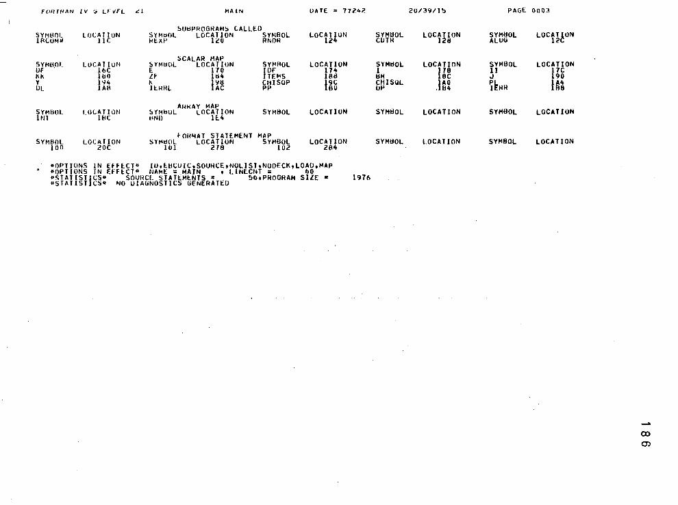
FORTRAN IV G LE~FL cl MAIN UATE = 77242

~UtiPHOGHAMS CALLED SYMI:lOL lOCATION SYMtHJL LOCATION SnlBOL LOCAT{ON I~CO~II llC l<t.XP teo RNOR 12

SCALAR MAP SYMH,OL LUCATIUN SYMtiOL LOCATION SYMHOL LOCATION Uf lt>C E 170 IOf lH KK ltlO lf }tl4 ITEMS lAd y l<J4 K 1'~8 CHISQP ~9C OL Al:l lt.HHL AC PP 80

AHKAY MAP SYMIHlL I.OCATION SYt~bOL LOCATION SYMI:IOL LOCATION lNl l~C tiN() lE.4

fOH~AT STATEMENT MAP SYMBOL LOCATION SYMtiOL LOCATION SYMBOL LOCATION

}00 20C 101 278 102 284

*OPTIONS IN EfFECT* IU,t.UCUICoSOUHCEtNOLISTtNOOECK,LOAU,MAP *OPTIONS IN EFFt.CT* NAME = MAIN t LlNE.CNT = 60 *STATISTICS* SOUHCl SIATtHt.NTS : 56tPROGRAM SIZE • 1976 *STATISTICS* NO UlAuNOSTICS GENERATED

20/39/l!l

SVMUOL CUTH

LOCATION 121!

SYMtiOL LOCATION 1 ps IJH 8C CIUSQL lAO IJP . B4

SYMtiOL LOCATION

SYMUOL LOCATION

PAGE 0003

SVMUOL AL06

LOCAT~ON 12

SYMBOL LOCATION II 17C J 190

nHR IU

SYMBOL LOCATION

SYMBOL LOCATION

-co m

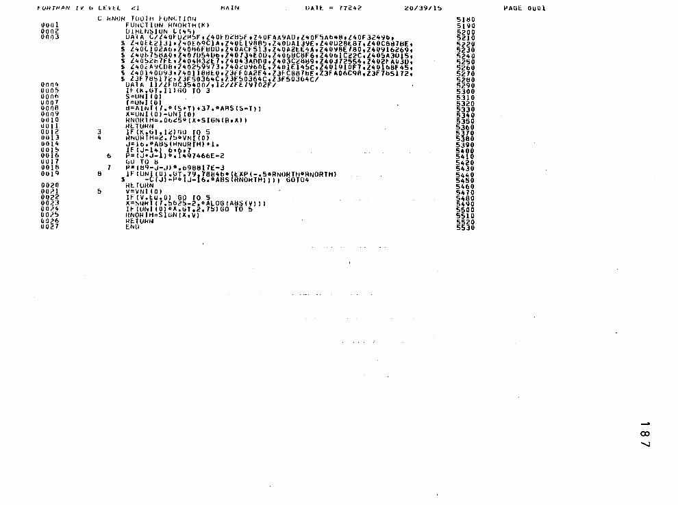
rU~TRAN IV b LEvtL ~l Ml\lN UATI:. = 77242 20/39/lS

0001 0002 0003

oo n'• ouo'> oonf> uoo7 uooe oon9 0010 0011 0012 0013 0014 0015 0016 UOI7 0018 0019

0020 oor.l 0022 00?.3 00?.4 00?.5 0026 0027

C HNOH TuOTtt fiJNCT JOt~ FUNCllON HNOHTHIKI UH-tlNSIUN L l4'i) UAlA C/L40tU~~~FtL40tO~HbFtZ40FAA9ADtZ40f5Ab48tl40F324Ybt

3 4

8

5

6

1

S z~oEt213ltl40£69ClAtl40~198B5tZ40UAl39Etl40U28l87,l40C6~7HEt $ L40Ll02AbtZ40~6fHUDtZ40ACf513tZ40A2tE4AtZ4098Ef60,Z4U916269t S L40b75tlAOtZ40fi>54UbtZ40734EOOtZ40otlC8f6tZ406lC22CtZ405A3015t S L4052h7FttZ404H3~t7t7404]AOOO,Z403C28H9tZ4UJ72554tl4U2tA03Dt S L40~A9CDb•Z402~9973t740~0Y60~,z40lEl45CtZ4019lOF7tZ401&8F45t S l40l40U93t/40ll8HEOtZ3FfOA2f4oZ3fC887bEtZ3FA06C98,Z3f7b5172t S LJf78517~tl3F50364CtllF50364C,Z3F50364C/

UAlA ll/lftiC35400/tl2/lFtf9702F/ It IK.6T,JliHO TO 3 S.:lJNIIOI T=UNI 101 d=AlNf((,o(S+TI+37,oARSIS-TII X=UNIIOI-UNIIOI HNOH1H=o0b~5~1X+SIGNIBtXII HtllJHN lfiK,GTol21HO TO 5 HNOHTH:2,7~~VNIIO) J=lbo*A~SIHNORTHI+lo 11' IJ-hl (n6t7 P=IJ+J-l)*ol~97466E-2 bU TO 1:1 P=I1:19-J-JI*.o96817E-J lfiUNIIUj•UT,79f781:14b*!EXPI•o5*RNOHTH*HNORTHI

i -CIJ -Po(J• 6o*ABS HNOHTH)III G0T04 HtTUilN V=VNIIOI IfiV.E.UoOI GO TO 5 X=SuHT(7,5b25-2o*ALOGIABSIVlll ll'llJNIIOioX,UTo2o751GO TO 5 I!NOIHH=SIGNIXtVI Ht TUHI~ t::NU

5Jtt0 5}90 5200 5210 5220 5230 5240 5250 5260 5270 5280 5290 5300 5310 5320 5330 5340 5350 5360 5370 5380 5390 5400 5410 5420 5430 54~0 5450 5460 5470 5480 5490 5500 5510 5520 5530

PAGE. 0001

-(X)

""-l

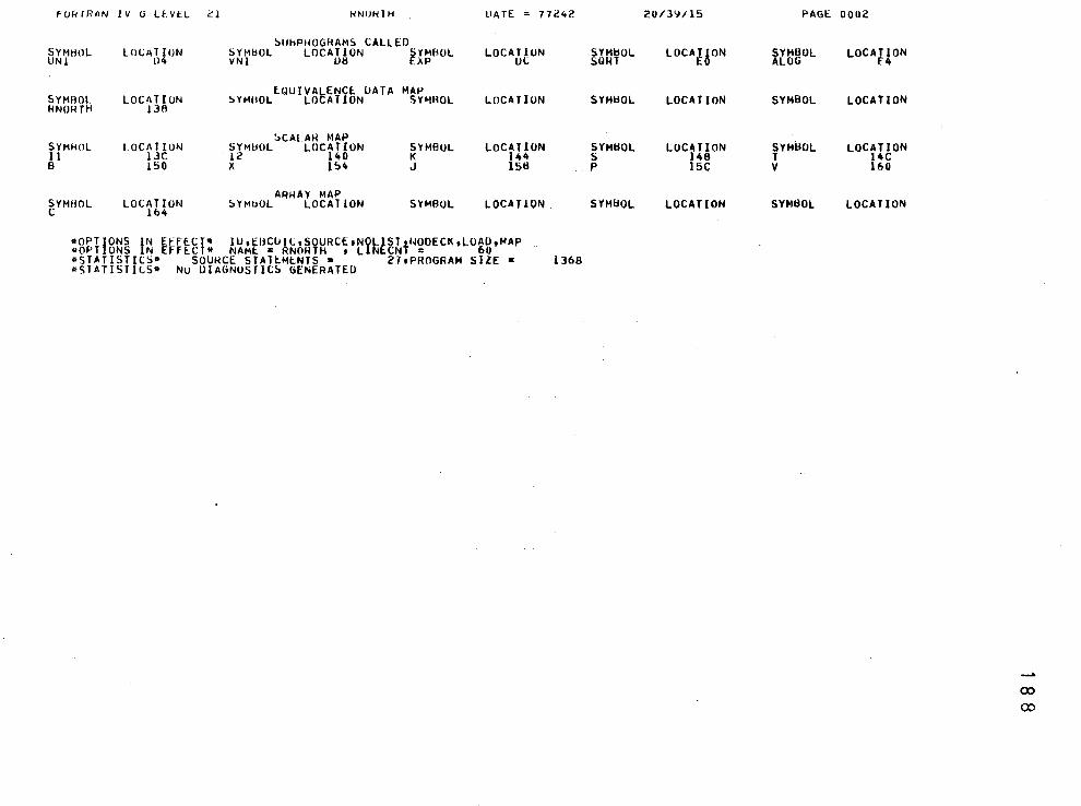
FUHfRAN IV G LEVEL 21 RNURTH OATE = 77242

~UhPHOGHAMS CALLED SYMtlOL LOCI\ liON SYMtlOL LOCATION ~YMHOL LOCATION UN! 04 VNI U!! J\P oc

lQUIVAEENCl DATA MAP LOCATION SYMBOL LOCI\TION SY~UOL LO ATION SYMHOL

HNOHTH 13A

SCAI AH ~lAP SYMHOL LOCATION SYMbOL LOCATION SYMBOL LOCATION 11 13C 12 140 K 144 B 150 X 154 J 158

A~HAY MAP SYMHOL LOCATION c lb4

SY~bOL LOCATION SYMBOL LOCATlOI\f

•OPTIONS IN EffECJ* IU,EHCU!CtSOURCEtNY~lST,NODECKtLOAD,MAP *OPT ONS N EfFlC * NAME : RNOHTH t L CN = 60 *STATISTICS* SOURCE STATlMENTS = 27tPROGRAM SIZE = 1368 *STATISTILS* No UlAGNOSTICS GENERATED

20/39/15

SYMbOL S<HH

LOCAHON

SYMtlOL LOCATION

SYMtiOL LOC~TION s 148 p 15C

SYHI;OL LOCATION

PAGE 0002

~YMBOL LOG LOCAJ!ON

SYMBOL LOCATION

SYMtiOL LOCATION T 14C v 160

SYMiiOL LOCATION

-(X)

00

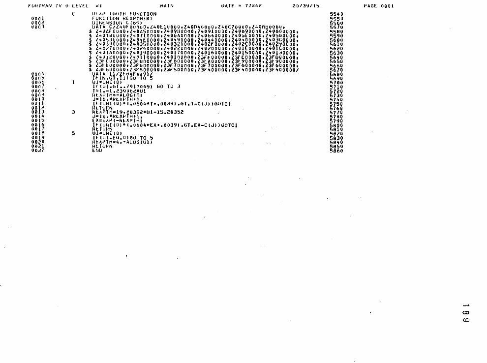
FURfHAN IV 6 LEVEL ~~ MAIN UATE 77242 20/3':1/15

0001 001)2 0003

0004 000~ OOOb ooo ., OOQii 000~ 0010 0011 0012 0013 0014 0015 0016 0017 0018 0019 0020 0021 002<'

c

3

5

HlXP lOUTH fUNCTION fUNCilUN N~XPTHI~l OHitNSIUN l 16'51 UATA l/l40tOU000tZ40ll0000tZ40040000tl40C700U0tZ•OR~OOOUt

$ L40Af0000tZ40ASOOOUt7409HUOOOtZ409lOOOOtZ40H90000tZ4UHOOOOOt $ l~01HUOOOtZ40TlOOOOtZ406AOOOOtZ40b40000tZ40~fOOOO,Z40~HOOOOt $ l~O~J0000tZ404E0000tZ4U490000tZ4U4400UOoZ40400000tZ403COOOOt S l40J~OOOOoZ40350000tZ40320000tZ402FOOUOol4U2COOOO,Z40290000t $ Z40r7000Ut740240000tl40220000tZ40200000tZ401E0000tZ401COOOOt ' L4UIA0000•740190000tZ40170000tZ4016UOOOtZ40l50000tZ4UlJOOOOt $ L4Ulc0000t74Pll0000t740lOUOOOtZ3ft00000tZ3flOOOOOtZ3fOOOUOOt $ lJtCOOOOUtl3F~OOOOUtZ3t~OOOOOtZ3tAOOOOOtZJt~OOOOOtZ3t~OOOOOt $ lJtHUOOOOtZJF~OOOOOtZ3F700000tZ3f700000tZ3F600000tZ3f600000t S lJfoOOUUOtZJf500000tZ3f~OOOOOtZ3f400000tZ3F400000tZJf400000/

OATA ll/ZFU4FA491/ IFIK.bTolliGU TO 5 Ul:UNIIO) H IUlobT •• "f9l70491 GO TO 3 T;l,-1,2J9~oc•u1 I~UI.PTH=-ALOG IT l J=lb ... RI:.XPTH+l, H IUI~l IOI*I.0604*T+,OOJ91,GT.T-CIJlluOTOI RL TURN RlXPTH=l9oc0352*Ul-l5,20352 J=l6o*HtXPTH+lo lX=lKI-'1-ki:.XPTHI IF IU~l101*1.~604*EX+.00391,GT.EX-CIJIIGOT01 HI:.TUHN Ul=UNliOI If IUloEU,OIGU TO 5 RlXPTH=4.-ALOGIUll Rt.TUHN E.tiO

5540 5550 5560 5510 5580 5590 56011 "i6l0 5620 5630 5640 5650 5660 5670 5680 5b90 5700 5710 5720 5730 5740 5750 5760 5770 5780 5790 5800 5810 5820 5830 5840 5850 5860

PAGE. 0001

00

co

FOHrRAN IV b LEVFL d HEIIPTH lUI TE = 77242

SlltiPAOGHAM~ tALLI-.D SYMllOL LiJC..~TION SH<1IHJL LOCATION S'YI1AOL LOCATION ~YMbOL UNl HC A LOb co EXP C4

SYMBOL lOCATION StMbOL HFXPTH U!

tQUIVAL~NCE UATA MAP LOCATION S'YMAOL LOCATION SY14t!OL

SYMHOL LOCATION SCALAR MAP

SYMUOL LOCATION SYMBOL LOCATION SYMI:IOL ll tC K ~0 Ul F4 T EX 100

MO!HAY MAP SYMHOl. LOCATION SYMbOL LOCATION SYMHOL LOCATION SYMt!OL c \04

*OPTIONS IN EFFECT* lUotbLUICoSOUACEtNOLISToNODECKoLOAOtMAP *OPTIONS IN E~FtCT* NAMt : HtKPTH t LlNECNT : bU osT•TISTIC~* SOUHLt STATEMENTS : 22tPROGRAM SIZE = *STATISTICS* NO UlA6NUSTJ<.:S bENERATEO

1076 '

*STATISTICS* NO UlAtiNOSTJ<.:S THIS SlEP

20/3~/l!)

LOCATION

LOCATION

LOCATION Fa

LOCATION

PAGE. 0002

SY1460L LOCATION

SY14t;OL LOCATION

SYMt;OL LOCATION ,J FC

SYMBOL LOCATION

co 0

,_ .u (/)

<( _,_ N< ... c .c;

wa:o Zt'\11-

~~0 ..0·.! ...... ,:, :\J~

OCI-< .-.­....... z ..:.....&J~ .... ,..,w u-..:x; y_::,n :!. VI v, <(

ll: :n Z:.:l>­;:,..,:,:) -...:r..JJ .... :::> ~ ... ~- .. , "'­:r-x

OZ..; -:::. ~--::::

""-5Z .<! VI ~ ...... <I:...J::> .-::::=. Z-<t

"' ;;. z '"' -' <(

I Z l) " "" ~ ... ~

~

1 9 1

1 9 2

0 a-'"' "" 0 ,._ ,.., 0

:1>

co (\j :1> 0

:c

.::> -c. .,. ..., ~

:::> ,._ <C (\j

Ln

:::> .n .n "' .,. e .,. . 0 ..... .

II .-: ::<: c • ::.on ..a.J-~ ..;u..; J::Z:::) ~·_;

:t:< ...... > c

C>-c.r....,a;: ....... "" l.u:...J~ J:.o.IZ ~.:;c..::. .o..J.li(O ::l..J.ll

••• ~0HI/NtHGt 5{3~-SHl,VlN l•MOU 4• CUNIHOL STATEMtNTS SOHT FltLil5::Ct:0,7,fltA•f>7,7,~ltAl

lGHPJ6I - H = ~1 IGHOJ7I - G: 1116

IGH038l - NMAX APHOX EUUAL 3000 GH0701 -tiLt Silt IS NUl SPECIFilU lGH04~l - fNU SONT PH . IGH049l - SKIP MlNbE PH 1GH0541 - HCO IN lOOOoUUT 1000 l6h052t - ENU OF SONTIMtRUt

OATt" 77.242 ......

-!'

-co w

CIHSQP= Cit I Sf~P= CH 1 sew= Cti!SIW= CHfS()P= CH SUP= CH1SQP= l:UlSUP= CHIS()P= CH SUP= CH1SQP= ChlSQP:; CIHStW= CH 1 sew= ClllSQP= CUISQP= CfllSQP= cu 1 sew= CHi SOP= CHI<;IH'= CHISQP= CH1StJI-'= CH1SQP= Ctil SQP= CUISQP= CH}SI)P= CUISQP= CUlSQP= CHISQP= Clll SeJP= CIH srw= CHlS!lP= CHfSQP= Cli SOP= CIIISQP= CHISQP= CIHSQP= tHISQP= CH1SQP= CH1StJP= CHlSQP= ClllS()P= CH!SQP= Cll1 StJP = CHISeJP= CH1SOP= CH1SQP= CHISQP= CHISQP= CHJSQP= CHlSiH'= CH1SIW= CH!SQP= CIIISQP= CHISQP= CHI SOP= CH1SQP= CH}SQP= ClflSQP= CHlSQP= CH1SOP= CHI!>QP=

1. coo o 1.H000 2.0000 2.ouoo 2. 00110 2.oouo z.oouo ?.oouo z.oooo 2.2ouo c.2ouo 2.2000 2.6000 2.6000 2.6000 2.6000 2.6000 2.6000 2.6000 2.6000 2.HOOO z.l:looo z.eooo 2.1:loJO 2.eooo 2.!:1000 2.1l000 J.oooo 3.oooo J.oooo :3.11000 J.OOIJO 3.2000 3.2000 3.2000 3.2000 3.2000 3.2000 3.2000 3.2000 3.4000 3.4000 3.4000 3.40~0 3.6000 3.6000 3.6000 3.6000 3.6000 J.f>OOO 3.sooo J.flOUO J.flOOO 3.H000 :i.E!ooo J.HOOO J.llooo J.auou J.Boou 3.8000 J.eoou J.HOOU

P=O.UU'JUl P=U.Uc'J~C' P=U.O'+U1f> P=0.04U1!> P=u.U'+Ulu P=U.U'tU b P=O.O'+Olb P=ll.O'+IJlb P=O.O't01o P=O.O::ii'U~ fJ=O.U~.?O~ P=O.O!:J.:O!:i P=O.Od0b2 P=O.OdiJbc P=O.Ot1062 P=O.Ot!U6~ P=O.Od1J62 P=O • OtHl62 P=O.Ot10b2 P=O.OtiObc P=0.0~7l3 P=0.0\17 J P=0.0\1713 P=o. 0':1113 P=0.0'>~7}3 P=O.U'l/7 3 P=O.O'll7l:i P=O.l1500 P=O.f1!:JOO P=O• l!:JOO P=O.l!SOO P=o.ll~oo P=0·~~4l0 P=o. 3<+ o P=O.IJ4l0 f'=O.lJ410 f'=0.134l0 P=O.lJ'+ 0 P=0.1J410 1'=0.13410 P=O•l~430 P=O. !:1430 r-::0,1!:1430 P=0.1!:1430 P=O.l/S<tll P=U.1/!:14tl P=U.l7!>'+tl P=0.17!:J4b P=0.1-f!:l41:l P=O.l7!::>41:1 P=0.1 'H50 1'=0.1'17!:.0 P=U.l\17~0 P=u.l'i7!>0 P=u.1'175u P=0.19"T!:>O P=O.l'i750 P=U.l'i7Su P=O .I 'i 150 P=O.l'175U P::O.l\17!:>0 P=O. 'i75U

UtN=O.Oc'JO 1Jt:.o~=U.04 70 uu~=o. osr:.J L•LH=O • 0553 UU'I=I).0~53 ~~~-11=0. 0553 ou~=o. 0553 IJI:.tl=O • 0553 UtN=0.0553 l>lN=0.0636 l>ll'-l=0.0636 l>~.N=O • 0636 IJEN=O.OHO IJEN=O.O"T90 IJI:.N=0.0790 UEN=0.0790 UtN=0.0790 Dt:N::0.0790 lJHI=0.0790 Uf.lt=O • 0790 UlN=O.Oti60 UlN=0.086(1 lJ£N=O.Otl60 llt.N=o. 01:160 lJEN=0.0860 Ot:N=o.o860 lllN=O.OR60 IJlN=O.O'J25 OHI=O • 0925 1Jt.N=o,o~25 lllN=0.0925 UtN=0,0925 OI:.N=0.09A4 lJI:.N=0,0\184 Ul:.r.=0.0984 LJtN=o.o~84 lllN=0.0984 UI:.N=0.091!4 LJt::N=0.0984 I.JEN=0.0984 IJtN=OoJ036 LJ~N,.O. 031> IJI:N=0.103b UEN=0.1036 Llf_N,.0.108f OI:.N=0.101:l l>E.N=O •l 081 UlN,.O. OtH Ot.tt=O.l081 Ut::N=O.IOtH U[i~=0.)}20 OE.N"'II•ll20 OI:.N,.O.ll20 l>lN=0.1120 UI:N=0.1120 IJf:N=O .1120 LJE.N=O.ll20 UI:.N=O.ll20 UI:.N=Ooll20 OEN=O.tl20 UI:N=O•tt20 UEN=O.t 20

II:.I<H-"0 1l~H;:O llHR=O 1l~<k=O

IE Flk=O lFIH=O

llRI<=O ll:.k!<=O

II:.Hk=O lHH=O

llPH=O ltHR=O lt:.RR::O llRR=O li:.RH=O llRH=O n~n~8 11:.RR=O ltHk=O

II:.RR=O lRH=O

l lRH=O E.RR=O

llHR=O llRH=O

l lRR=O ERR=O

l lRR=O E.RH=O

lERR=O lERR=O

IERR=O lRH=O

II:.RR=U lERR=O

l t;HR=O EJ.Ik=O

llRH=O IE.RR=O

IERR=O lRR=O

llRR=O llRR,.O

l lRR=O I:RH=O

llRR,.O llRR=O

l lRR=O tRR=O

IERR=O 11:.RH=O llRH=O lt:.RR=O lERk=O llRR=O llRH:O H.PR=O lEPR:O IERR=O

IE.RR=O t.RR=O

CHlSQL= 1.2Ut>l CHISQL= 1.8112 CH1S<JL= 1.'HAO CHISOL= 1.~760 CHISOL= 2.0115 C11IS!JL= 2.0283 CHISOL= 2.0bl6 CHIS!JL=- 2.0618 CHlSOL= 2ol024 CHIS!JL'" 2.1601 CH1SOL= 2o1763 CHISOL= 2.234? CUISQL= 2.6161> CHlSQL= 2.6334 CH1SOL= 2.6334 CHISOL= 2.6!:117 CHfSQL= 2ot>!:ll7 CH SOL= 2.6!:1 1 CUIS!JL= 2ob!:l17 CHISOL= 2.7884 CUfSOL= 2o6tll3 CH SOL= 2.61i 3 CHlSQL= 2.8337 CHISQL= 2.tl337 CHfSQL= 2.9887 CH SQL= 3o0222 CHISQL= 3,02?? CHISQL= 2.9039 CHfSQL'" 2.9600 CH SOL= 3.1708 CHISQL= 3.1708 CHIS<)L= 3.2'+48 CHf'iQL= 3o2l62 CH SOL= 3,2 62 CHJSQL:a 3.2162 CHISQL• 3.3071

~~nat~ ~:3H l CHISOL= 3.3711 CH1S!lL= 3.41 1 CHJS(JL= 3.3~49 CH SOL= 3.3!:)49 CHlS!lL= 3.Jb30 CH15GL= 3.5074 CHfSOL= 3 0 5370 CH SQL= 3.7535 CHJSQL= 3.7941 CUISOL= 3,1941 CHJSQt:: 3,1'141 CHISQ = 3.9185 CHISQL= 3.4869 CIU StiL = 3 • !:)499 CHfSOL= 3.!.i778 Ot SOL= 3. 7094 CHISOL= 3,7597 CHlSOL= 3.8060 C11fSQL= 3.8060 CH SQL= 3.8283 CHISOL= 3.8740 CHISQL" 3.9203 CHfSQL= 3.9762 CH SOL= 4.1006

P=0.0092l P=0.03045 P=0.0389~ P=0.0389!:) P=0.040AO P=0.04174 P=0.04JE-6 P=0.04366 P=0.04604 p:;0,04955 f':O.OS068 P=0.05425 P:0.08l93 f'=0.0832U P=0.0832tl P:0,08475 P=Oo08475 P=O.OA475 P=O.OB475 P:0,09613 P=0.08716 P=0.087 6 P=0.10006 P•0.10006 P=0·~~395 P=o. 706 P•Oo 1706 P=o. 06?6 P=Oof1}32 P=o. 3 23 P•0.13123 P=O.IJA53 P=o. 3569 P=O. 3569 .P=0.13569 Pa0,1447B P=O.l513l p .. o. 5 3 · P=0.15132 P=0,15551 P=O,I4965 P=Oo 4966 P=o. 5254 P=O, 6556 P=0 0 16fl7l P=O.l923 P .. 0.19684 P=0.19b84 p .. o.19684 . P:0.2108~ P=0.16339 P=O•f700il P•o. 7309 P=0.1874c P•0.19300 P=0.19817 f'•Oo19817 P•0.20067 P=Oo20583 p:aQ.21109 P=0,21748 F-':0.23188

UtN=0.0232 Ot.N=0.0475 UlN=0.0544 OlN:0.0544 OI:.N'l'0.0558 OEN=D.0565 UI:.N=0.057'i OEN=0.0579 oE.N=o.o596 PE.N=0,0619 OEN•0.0627 OlN"'0.0649 UI:.N=0.0796 DEN=0.0802 OEN=0,0802 Ot.N•0.0809 OEN•0,0809 Df.N;:0,0809 UE.N=0.0809 Ot.N:0.0856 OE.N=0.08f9 OEN=o.o8 9 OlN•O.u872 OE.N=0.0812 OE.N•0,0922 OI:N:a0.0932 OfN=0.0932 OE.N=0.0895 OE.N=0,0913

- OE.N=O • 0975 OI:.N=0.0975 OE.N=0.0996 Ot:,N=0,098B OEN=0.09A8 DI::N=0.09BB OEN=0,1012 OI:.N=8•1029 OE.N:a • 029 OEN:::0,1029 OlN:::0,103B OE.Na8•1025 - DEN• • 025 OlN=O.l031 OlN•Ool061 Ot.Nao,I067 DEN=o. 111 OlN=Oolll9 Ul:.N=0.1119 OE,N=O•lfl9 DEN=o. 40 OI:.N=0.1056 OEN=O.l070 DfN:::o.l076 OEN=O, 103 OlN=0.1Jl2 Ot.N=o.1 21 Ot.N=O•f121 ut::N:::o. 12s OlN=O•fl32 Ul:.N=O. 140 UlN=g•fl48 OEN= , 65

1ERR=O lERR=O lERR::o ll:.RR=O

IERR:O ERR=O

lERR:O lERH=O

II:.RR=O ERR=O

ltRR=O

IERR=O ERR•O ERR=O

IERR=O IERR=O n~~:g IERR•O IERR=O

IERR=g ERR=

IERR=O JERRaO

IERR•O ERR:O ERR•O ERR=O

IERR=O ERR=O

IERR=O IE.RR=O

IERR=O E.RR=O

IERR=O lERR=O

IERR=O ERR=O

lERR=O lERR=O

IERR•O ERR=O

1lRR=O IERR•O

IERR•O ERR•O

lERR=O IERH=O

IERR•g ERR•

IERR:O ERR•O ERR=O

IE.RR=O IERR=O IERR•O

IERR=O ERR=O

IERR:O

IERR=O ERR•g ERR=

CELL FREQ l2 9 11 10 8 10 11 9 CELL FREQ 10 9 12 11 12 8 10 8 CELL FREQ 9 11 8 0 13 8 10 11 CtLL fHEQ 11 ll 9 3 10 8 11 10 CELL FREQ 8 9 f1 ·a 11 9 12 ~2 CELL FREQ 10 9 0 10 3 10 7 1 CELL FREQ 11 10 7 ~ 12 9 12 0 CELL FREQ 12 9 9 10 12 7 11 10 CELL FREQ 10 8 11 11 11 7 10 12 CELL fREQ 8 10 8 0 2 9 3 0 CELL fREQ 11 13 11 -~ B 9 8 11 CELL FREQ 8 f1 12 10 11 8 8 12 CEtL fREQ 9 c 11 ·a f2 8 12 8 CE L fREQ 10 12 0 10 3 1 8 10 CELL fREQ 1~ 1 10 13 10 10 12 8 CELL FREQ 9 11 10 8 13 1 11 11 CELL fREQ 10 13 11 9 II 6 7 fl CELL fREQ 1 8 9 10 1 13 CELL FHEQ 9 1 13 1 10 8 11 CELL fREQ 10 10 10 lo 11 6 10 l CELL fREQ lo 11 8 ·9 f1 8 14 9 CELL fREQ 0 B 8 4 11 9 9 CELL fREQ 12 10 11 9 0 1 8 CELL FHEQ 8 3 12 10 10 1 11 9 CELL fREQ 6 11 fO 9 13 10 f1 10 CELL fREQ 12 9 1 11 2 6 0 9 CELL fHEQ 11 9 12 2 11 6 10 9 CELL FREQ 10 11 1 8 14 10 8 8 CELL fREQ ~3 9 9 1 13 0 9 10 CELL FREQ 3 9 10 10 2· 6 10 0 CELL FHEQ 10 6 12 10 10 9 10 13 CELL FHEQ 10 10 2 11 12 11 6 8 CELL FREQ f2 10 8 2 J3 9 9 1 CELL fREQ 2 2 9 3 0 8 9 7 CELL fHEQ 9 12 8 10 13 1 9 12 CELL fREQ 13 1 10 10 11 7 10 12 CELL fREQ 9 l3 11 12 9 6 10 lo CELL FREQ 11 2 9 0 10 9 6 3 CELL fHEQ 9 0 9 11 13 6 12 10 CELL FREQ 11 11 13 11 8 6 10 10 CELL FREQ 11 11 ll 1 14 9 9 8 CELL FREQ 8 9 14 1 1 9 11 CELL fREQ 10 8 13 9 9 1 11 3 CELL FREQ 11 1 9 13 10 1 12 11 CELL fREQ 12 9 14 11 9 7 10 8 CELL fREQ 9 13 2 0 12 6 9 9 CELL fREQ B 6 13 f1 12 11 9 10 CELL FREQ 10 9 2 J 11 8 6 11 CELL fREQ ~3 9 ll 1! 12 6 10 8 CELL fREQ 1 10 1 12 6 12 7 CELL FREQ 9 12 9 f5 8 9 9 CELL fHEQ 10 1 15 10 0 8 8 8 CELL FREQ 9 9 15 7 9 10 10 11 CELL fREQ 11 f1 12 8 14 8 8 8 CELL FREQ 10 4 11 8 f2 B 1 fO CELL FREQ 13 1 8 11 1 9 8 3 CELL FREQ ll 9 1 8 13 8 11 f3 CELL FREQ 9 14 11 1 7 1 0 CELL FHEQ 9 10 10 0 f4 6 9 12 CELL fRf.Q 6 13 9 9 0 9 II 13 CELL fREQ 10 9 10 f3 }2 6 8 12 CELL fREQ 7 12 2 _0 1 6 10 12

-co ~

CHISQP= LHlSUP= CHlS!lP= OtlSOP= CtHSoP= CHlSQI'= CHlSrW= cu J sc~P = CHI $(lP= CHJSQP= Cltl SCJP= CHI SOP= CHlSOP= l:IH SllP= CHI SOP= CHIS!1P= CHlSUP= CH Sill-'= CH1Srll-'= CHlS(JP: CIHSOP= Oil SO f.'= CH1SOP= cui sew= CHISilP= CHlSCW= ClllSllP= LHlSOP= CHISOf'= OtlSUP= Ct!lSUP= CHlSQP= CHlSt)P= Cttl Sill-'= CH[SQP= Ctt! SQP= CHfSOP= CH SUP= CIHSQP= CHJSQP= CHJSQP= CH1SQP= CHJSQP: CHI SOP= CHtSOP= CH scw= CHI SOP= CHI SUP= (;HI S(JI-'= CH SclP= CHlSQP= CHlSQP= CHISQP= Ctfl SclP= CtlJSQP= CHlS!lP= CHI SOP= Cti! sew= C~ll Sr)P= CtllSclP= CHJStW= tHlStlP=

4.0()(11) 4oOOOil 4.0000 4.11000 4.0000 4.0000 4.0000 4.0000 4.0000 4.0000 4.0000 ... oooo 4.0000 4.2000 4.<'000 4.2000 ... zooo '+.2000 '+.2001) 4.4000 '+.4000 4.4000 4.4000 4.4000 4.4000 4.4000 4.4000 4.4000 4.4000 4.4000 4.4000 4.4000 4.4000 4.6000 4.6000 4.t-uoo '•·6000 4.6000 4.6000 4.8000 4.8000 4.8000 4.8000 4.8000 4.8000 4.H000 ... nooo 4.8000 4.8000 4.1:1000 4.11000 4.111!00 4.HOOO 4.8000 4.Hooo 4.8000 4.8000 4.1'1000 4oHOUO s.oooo s.oooo s.oouo

P=U.ccUc? P=O.t!t!Ut!? P=O.t!t!U2c P=O.ct!Oc2 P=U.2cli22 P=O.ct!022 P=o.zcozz P=ll.220c2 P=0.22022 p=o.zcoz;,> P=O.i:!2022 P•O.c/.022 P=0.2202C. P=O.c'+3!:>2 P=0.24352 P=O.c4J!>c P::0.243~2 P=O.c'+J~c P=ll.24353 P=0.2b7cH P=0.2o12t! P=0.2f>72ti P=0.2f>7t!ti P=0.2bf2t! P=0.2bl2b P=o.cb7c& P=o.2ofcll p:o.2b728 p::o.zo·/28 I'=O.C::f>7t:!t! f'=0.2o72ti P=o.zorc:t~ P=0.26128 P=O.c'i136 P=O .c':ilJo P=0.2'11Jb P=0.2'11Jo P=O.C::'Il3b P=ll.2'1l3o P=0.3l!:>b4 P=0.3l!>64 P=O.Jl!:lo4 P=o.Jl!>ott P=0.3l!>f>4 P=0.31!:>b4 P=o.3l!:>t>4 P=O •. H 564 P=11.3l!>64 P=0.31!>64 P=U.J1!>64 P=0.31!>b4 P=O.Jl~o4 P=O.Jl!>b't P=U.Jl!>64 P::U.Jl!:>b4 P=O.Jl!>b'l P=O.Jl!:>b4 P=O.Jl!:>o!> P=U •. H !>6!> P=O • J'•UOtt P=0 • .34U04 P=O.J'+UU'l

IJtt•"'Oo]J5? LJtt.=Ooil52 UE.N=!lo1152 U~N=0.1152 Ut:.r~=o ·1152 UE.N=O.ti52 UE::N=Ooll52 lllN=0.1I52 UEN=O.ll52 UE.H=Oo1152 UEN=0.1152 U[N=0.1152 UI:.N=O•fl52 UtN=O. 77 UEN=Oo1177 Ut:.N=0.1177 UEN=O•ll77 OF.N=o. 77 Ul:.l~=ll.1177 UtN::0.1197 llEN=O•Il97 UEN=O • 97 UE.N=0•1197 UFN=O.tl97 IJlN=Ooll97 UtN=0.1J97 IJlN=O •1197 IJlN=Oo1l97 UlN=O•lf97 UlN=Ool 97 UEN=O•ll97 · UEJ4=0 •1 97 UUI=O•f197 UlN=O. 210 UU.1"0o1210 UI:.N=0.1210 Ul~I"'U•I210 UI:N=O. 2 0 Uf.N=0.1210 UlN=O.l21fl UlN=Ool2l8 Ut:N=O. 2 8 LJI:.I~=0.121tl UU4=0.1218 UI:::.N=O.f2f8 IJE.N=O. 2 fl UlN=IJ.1218 UlN=0.1218 lllN=o.J2fB u~:t~=o. 2 8 UlN:::O.I218 UI:.N=0.1218 Ut.N=Ool210 IJI:.N=O .1 c18 lli:.N=O.l2l8 UlN"'Ooi218 uu~:o.1218 UE.N=O.t2lk IJI:.N=O.t21tl UtN=O.J220 uu~=o .1220 U[N:0.1220

ltRR=O 1£1Hi'=O ltRH=O llRH=O li:.RH=O ll~H=O llPH=O llRH=O llRR=O IE.RH=O lE.R~=O llRH=O

l lf!H;8 lRR=

llRH=O llRk=O

l lHH=O f.RH::O

l lRR=O lRH=O

lf.RR=O lRk=O

J[RH=O llRR=O H.RR=O llRR=O lf.RH=O lf.RR=O IE::RH=O lf.RH=O

l lRR=O lRR=O ll~k=O llRR=Il ll~H=O llHR=O

l lRk=O lRH=O

IERH=O llRH=O

flRk=O f.Rt<=O

llRR=O llRH=O

l f.RH=O lR~=O

llRH'"O II:.RR=O

l i:.RH=O tRH=O

li:.Rk=O llRR=O

II:.RR=O lRH=O

If.RH=O llRR=O llRR::O lERH=O llRR=O llRH=O

II:.RR=O tRH=O

CHISQL= 3otHI59 CHISQL= 3.~1!81 CHJSQL= 3.'11:181 CHISOL= 4.0103 CHISOL= 4 0 0744 CHISI~L= 4o1125 CHfSOL= 4.1150 CH SUL= 4.1150 CHISOL"' 4. 430 CHISOL= 4 0 430 CHISOL= 4.1765 CH1StlL= 4o4b60 CHISOL"' lto41:142? CHISOL= 4.210 CHISOL= 4.2970 CHISOL= 4.2970 CHJSOL= 4.3433 CH SOL• 4.3'19? Clll SilL= 4 • 3992 CHlSOL= 4.2235 CHISilL= 4.3!:193 CHISOL'" 4o3'128 CHISUL• 4.4334 CHISOL= 4.4334 CHfSQLz: lt.49it9 CH SOL= 4.5254 CHISQL= 4.5660 CHIS<~L= 4.5660 CHISOL• 4o5660 CHJSQL= 4o649A CHISOL= 4e6498 CHISOL= 4o6'+98 CHISOL= 4.8789 CHJSOL= 4.:11:133 CHISQL= 4o5596 CHJSQL= 4obc36 CHfSO(= '+.7704 CH SQ = '+.1&62 CHISQL= 5.0609 CH1SQL= 4.3572 CHfSOL= 4.60i9 C~l SOL= 4o6'll 4 CHISOL• 4 0 69 4 CHISOL= 4.7320 CHfSQL= 4o71:123 CH SI~L = It • 8461 CHISilL= 4.8463 CHISOL"' 4.8463 CHISQL• 4.8463. CHJSQL: 4od463 CHlSOL= 4.'1021 CHJSOL= 4e9481t CHISI~l= 4.9484 CHJSQL= 4.9707 CHlSilL= lte9707 CHISOL= 5.1693 CHJSOL= !:I.Z278 CHJSOL• 4.lb0q CHISOL= 5.<!114 CHlSQL= 4.!:1295 CHJSQL= 4.8566 CHJSOL= 4.~430

P=0.2o'ne P=0.218A5 P=0.218A5 P=0.22142 P=0.22fl83 p::O.l3327 P=0.23355 t>=0.23355 P=0.23684 P=O.i!3684 P:o0.24076 1'=0.27519 f'=O • 27139 P=0.24478 P=0.25500 P=0.25500 P=0.26051 P=0.26718 P=0.26718 P:o0.24630 pco.Z624} P=0.2664 Pa0.2712 P=0.27127 P=0.27867 P•0.28235 p:ao.28725 P=0.28725 P:a0.28725 P=0.2973~ P:ao. Z91:J9 P•0,29739 P=0.32526 P=0.26527 P=0.28647 ..... 0.29421 p:=o.Jl2o4 P=0.3 396 Pao.34747 P::0.26216 P=0.29207 P=0.30243 f':0.30243 P=0.30736 ~;8:UU3 P•0.32129 p::O.J2129

~=s:Htn P::O.J2810 f->::0.33374 P=0.33374 f'::O.l3646 P=O.J3646 P=0.36069 p::o.36781 P=0.31088 P=Oo37312 f>::O.ZA2A4 P=O.J2254 P=0.33308

OtN=O.ll3'+ Lli:.N:::0.1150 UlN"'0•1f50 OlN::o, 53 OlN=O•ff62 UlN=O. 67 OlN=O•ff67 Ut.N=o. 67 UlN::0,117f UlN=o.ll7 DlN•0.1175 OlN•0.1202 OI:.N=Oof20J UlN:otJ. 179 OI:.N=O.f188 Of.N=o. 188

H~~:8:fU~ OEN•O. 197 OlN•O.ll80 OlN=O•fl9J UI:.N=u. 96 UI:.N=O. 199 OI:.N=O, 199 Ot,N•0.~204 OEN=O. 206 DEN•O, 208 OlN=o. 208 Ot.N•O,l208 Ot.N=o. 213 OlN•O.l213 OI:.N=o. 213

Bt~=&:u~g DlN=o,l208 OI::N"'O• 211 Of.N•O•l2f7 Ut.N=o. 2 8 OlN=Oo1220 UE.N=0.1l93

Bt~:8:~~l2 OlN•Oo 214 OI:.N•O. 216

Bt~:s:UU UEN=o.t219 Dt::N=0.1219 Ht~:s: l~U OE.N:oO.l220 OlN=0.1?.20 OI;.N=O,l220 U£N=o. 220 UI:.N=Ool2?.0 UlN=0.1219 IJI::N=Ool2f7 Ot.N=0.12 7 OlN=Oo1216 Ut:N=Oo1206 OI:.N=Ool219 OlN=0.1220

1ERR=O IERR=O

IERR:O I:.RR•O

IE.RR=O 1ERR=O

IERR=O ERR•O

IERR•O ERR=O

IERR=O IERR•O

IERR•O ERR::o

IERR=O IERR•O

u~~=s IERR•O IERR•O

IERR•O ERR=O

IERII•O JERR•O

II::RRo:O ERR•O

IERR::O ERR=O

IEPR•O I::RR=O

IERRo:O ERR=O

IERR=O 1ERR=O IERR=O IlRR::o

IERR•O ERR•O

IERR=O IERR=O

IERR•O E.RR=O

IERR=O IERR•O

IERR=O ERR=O ERR=O ERR:o:O lf~~:g IERR=O

IERR=O t::RR=O

II:.RR:O IERR=O IERR=O IERR=O JERR•O

IERR=O ERR=O

IERR=O ERR=O

CELL FREQ 13 lit 10 H ~ 1 10 9 CELL fREQ 13 12 IO 8 13 7 8 9 CELL FREQ 13 0 9 }2 f3 7 8 d CELL fREQ 10 1 ll 4 1 10 9 7 CELL fREQ 11 9 12 ~ 14 6 9 10 CELL FREQ 8 13 7 11 1 10 12 12 CELL FREQ 14 f1 6 11 11 10 8 9 CELL FREU 1 0 6 8 4 11 11 9 CELL FREQ 8 13 10 }1 13 6 fO 9 CELL fREQ 6 3 9 0 13 8 1 10· CELL FREQ 9 11 9 12 13 6 8 12 CELL FREO 13 0 9 1} 10 10 12 5 ~~tl r~~g ~~ 11 1 ~ 11 1x 1 ~~ ~ CELL FREQ 11 4 8 6 10 9 10 12 CELL FREQ 10 14 9 8 11 6 10 12

~~ll ~~~8 3 f1 fA 2 1~ 3 I~ fl C[LL FHEQ 8 0 l 8 11 6 12 ~ CELL fREQ 7 0 1 f1 1~ 8 8 10 ~~tl ~u~g ~~ 13 ~ ~ I J 1¥ ~ CELL fREO 12 11 14 11 lo 8 7 7 CELL fREQ 14 0 12 8 11 11 1 7 CELL FREQ 12 12 7 9 fl 7 12 8 CELL FREQ 0 8 12 9 3 6 J 9 CELL FHEQ 13 8 8 11 1J 6 0 11 CELL FREQ 10 11 6 8 13 8 11 3 CELL FREQ 11 8 13 8 lJ 6 10 11 CELL FREQ 12 9 2 7 3 10 11 6 CELL FREQ f3 6 12 ll 7 10 f2 9 CELL FREQ 3 10 7 2 11 6 2 9 CELL fREQ 12 11 6 ll 12 6 11 11 CELL FHEQ 9 9 d 7 9 2 5 CELL FREQ 10 7 9 ~ 13 7 11 14 CELL fREQ 1~ 9 11 ~ 13 6 9 9

~fll f~f8 tt ~~ 1¥ 9 ll 1~ ~~ 19 CELL FHEQ 6 J1 6 11 10 12 12 12 CELL FREQ 10 1o 9 9 7 9 16 10

~~t~ fH~8 1' 8 ' 1~ ll X 1 ~ 13 CELL FREQ 9 14 8 12 3 8 9 1

CELL FREQ 11 8 7 1:1 14 8 13 11 ~Ett fH~g IY 13 1 ~ 1 ~ 1I l 11 I~ CELL fREQ 6 9 14 11 9 8 J· 10 CELL fREQ 8 11 9 9 10 6 14 l CELL fRF.Q 1:1 11 10 13 14 6 9 9 CELL FREQ 9 8 3 11 9 6 14 10 CELL FREQ 14 10 10 8 12 6 8 12 CELL fRf.Q 8 9 13 12 13 11 8 6 CELL FREO 8 f3 8 13 11 6 9 12 CELL FREQ 12 0 11 11 4 6 7 9 CELL FREQ 6 11 12 14 11 10 7 9 CELL FREQ 12 9 10 10 14 5 9 11 CELL FREQ 6 10 fZ 13 II 11 11 6 CELL FREQ 8 11 0 9 6 15 10 CELL FREQ 11 9 8 12 13 5 10 12 CELL FHEQ 10· 8 10 8 16 8 11 9 CELL FREQ 11 9 12 9 10 7 7 l5 CELL fREQ 2 10 ~ 8 5 6 19 0

-co U'l

LHJS 1W CHlSilP CH l StlP Cttl SQf' CHI SOP CHlSQP CHI SllP CH1SQP CHISQP CH1 SllP CHISQP Cl~ I SQP CHISQP CHISQP CIHS!lP CHIS!lP CHISQP CHISIW CHISQP CHISQP CtlfS!lP CH SrJP CHISQP LHISQP CIHSQP CtllS'lP CHISQP CHI SOP Ctl f SIJI' CH SQP CHI SOP CH1SQP CtHSQP Clll SOP CHISQP CHISQfJ CttlSrW CH}SIW CHlSQP CHI SOP CHlSQP CHI SOP CH}SQP CHJSQP CHIS•H' CHlSQP CHI SOP CHlStW CIHSOP CH}SQP Ctll StlP Clll SQP CHI '>fJI' CH SIJP CHlS!lP CHlSQP ClilSQP CH Sr~P CHISflP CIHSQP CHlsnr CHlSflP

s.oooo s.oooo s.oooo !:l.oooo s.oooo !:l.oooo s.oooo s.oooo s.oooo !:l.oooo 5.oooo !:1.2000 5.2000 5.2000 !:1.2000 5.20011 5.2000 5.2000 5.2000 5.2000 5.2ooo 5.2000 ~.21100 5.2000 5.2000 5.4000 5.4000 5.4000 5.4000 5.4000 5.4000 !:1.4000 5.4000 .,.4000 5.4000 !:>.4000 !:>.4000 5.4000 5.4000 5.6000 5.1)000 s.6ouo 5.6000 5.6000 5.6000 5.6000 SobOOO s.&ooo 5.6000 5.6000 s.noou 5.6000 5.6000 !l.oooo 5.6000 s.Hooo s.Hooo 5.flCJOO s.noou s.aooo s.uooo !>.fiOOO

P=O.J4004 I-'=Oo341l04 P=O.J4004 P=O.J4U04 P=o •. H uo4 p:(I.J4004 P=u.34UU4 1'=0.34004 P=O.J4004 P=0.34UU4 1-'=0.34004 p::o.J644J P=O.Jo443 P=0.3blt4J P=O.Jo443 P=O.Jb44J P=O.Jb443 P=0.3b443 P=0.36443 P=O.Jb443 P=0.36443 P=0.3o44J P=o.36443 P=O.Jo443 p::o.3o<t43 P=O.JtHH3 P=O.Jil873 P=0.38~l3 P=O.JI1til3 P=0.3HH73 P=0.3i:IA7J P=O.Ji:ll:\73 P=0.311813 P=o. 38813 P=O.JI1f!73 P=Oo3!H!7J P=0.361:l73 f'=O.Jt181J P=0.311H73 P=0.4121l5 P=0.41~H!:> P=0.412ti!l P=0.41i::'H~ P=0.4121l5 P=0.4121.l!:> P=Uo'+1285 P=0.41265 P=o.4lctl~ P=0.412115 P=0.4121l5 P=llo 41 i::ti!.> 1-'=0.412115 P=Uo'+12115 f>=0.4121l!:> P=o.4lcH~ P=o.4J671 P=Oo4J671 P=0.4J&11 P=0.43o71 P=o • 4.jo II P=U.~Jb7l f'=0.4J671

IJU•=O.l220 UtN=0.1220 IJI:.N=O ol?.i?O 1JfN=0.)220 I.JtN=O.l220 lit.N=Oo12i?O lii:.N=Ool2?0 [Jf_N=O.l220 U~N=O.l220 Uf.N=O.l220 Ut:N=O.l220 liEN=O.l218 IJEN=Ool218 UHI=Ool218 UI:.N=O.l218 1Jft,=0.1218 UE.N=O.l218 IJEN=O.l218 U£1~=0.1218 li~N=0.1218 UI:.N=O•f2l8 UI:.N=o. 2 8 UI:.N=O.l218 UlN=O.l21A Ut:N=Ool218 UI:.N::0.)211 UtN=Ool211 UI:.N=O.l211 IJI:.N=0.121f IJI:.N=Oo121 Ul:N=11.1211 Uli~=0.1211 lli:.N=0.1211 llHl=O.J211 1Jf.N=O.l21f IJEN=0.121 UI:.N=O.l211 IJE.N=0.1211 lJEN=Ool211 IJI:.N=Ool200 UI:.N=0.1200 Ut.N=0.1200 1Jf:N::0.1200 UEN=O.J200 IJI:.N=O.l200 ut-.N::o. 200 UEN=O.l200 DI:.N=O.l200 DI:N=0.1200 IJI:N=0.1200 L'I:.N=0.1i?OO UEN=0.1200 UE:N=0.1200 Ut N=O .1200 Uli~=O .1200 uu.::o. 1186 U£1PO oll86 UH~=o o1 !16 UEN=0.)}86 (Jt:!>.=0.1)86 1Jf:N=0.1186 Uti~=0.)186

II:.Rk=O 11:.~~=0 IE~~=Il H.RR=O ltRk=O li:.FIH=O HR~=O II:.PH=O IERH=O H.RH=O II:FIH=O II:.RH=O IERH=O IE.RR=O llRP=O llRk=O 1lRR=0 It:Rk=O lt:RR=O lEPR=O l lRR=O

l:Rk=O llRR=O llflR=O IE.Rk=O

ERR=O IERk=O llRk=O H.RHo::O lt.Rk=O HRk=O 1ERH=O lERI-!=0 1ERR=O It:flk:O 11:.1-!R=O li:.RR=O lt:RR=O 1t:RH=O JE.RH=O IERR=O llRH::O llRH=O H.RH=O tE.RR=O

lRI-!=0 IERR::O H.RH=O lERH=O llPR=O IE.fHi=O 11:.RH=O IERko::O

I:.Rk=O 1ERH=O IlRH=O IERH=O

lRR=O IEHR=O IERR=O

I[RR=O t.l'lfl=O

CHISQL= 4.'lol?. CHlSflL= 5.1025 CHISQL= !;.l52R CHISf~L= 5.15211 CHJS<~L= 5.152fl CIHSQL= 5.1~91 CHlSflL:: ~.3920 CH1SQL= 5.3':120 CHlSflL= 5.4099 CHJSQL= 5.4383 CHJSQL= 5.5627 CHlSQL= 5.1266 CHISQL= 5.143'3 CHlSQL= So143'3 CHISOL= 5.21191 CHISQL= !:1.2891 CHlSOL= 5.3196 CH1St1L= 5.3937 CHISQL= 5.42}8 CH1SQl= 5.421R CHlSflL= 5.5':123 CHISQL= !J.bl02 ClilSflL'" 5.6~44 CHISQL= 5.7448 CHfSQL:a 6o1b40 CH SQL= 5.0029 CHlSCJL= 5.1552 CH1SQL= 5o3660 CHfSQL= So4559 CH SQL" 5o4~40 CHlSQL= 5.5175 CHISQLo:: 5.5200 CHISOL= 5.5535 CH1SQL= S.!HS8 CHfSQL= 5.7185 CH SQL= 5.1185 CHfSOLo: 5o8207 _ CH SQL= 5.8835 CHfSQL= 6.3461 CH SQL= 5o2032 CHISQL= 5.5663 CH1SQL= 5o5719 CHJSQL= 5.5877 CHISQL• 5.5877 CHfSQL• 5.6166 CH SOL= 5.6380 CHJSQL= 5.7020 CH1SQL= 5o 7020 CHfScK"' 5. ·ro2o CH SOL= 5.7707 CHlSflL= 5.9747 CHISQL• 6.0434 CHfSQL= 6.0434 CH SQL:: 6.1272 C~llSQLo:: 6.60?.2 CH1SQL= 5o3tl53 CHfSQL= 5.31l5"3 CH SOL= 5.4J55 CHJSQL= 5.6285 CHlSOL:: 5.7<t84 CHISfJL= 5.1{22 CHISflL= s.s 70

P=Oo335]0 P=0.35254 P=Oo35868 P=0.358!>8 P=0.35fl68 P=0.36412 P=0.38776 P=0.3877n f'=0.3A992 P=0.393~6 P=0.40837 P=0.35548 f-'=0.35752 P=0.35752 P=0.375?.7 P=0.37527 P=0.37898 f>o::0.38797 PaOo39137 P=0.39137 P:&•4f19!? P- .4 0"1 P=0.42415 P=0.43015 P=go41926 P= .34039 pao.35897 P:o0.38460 P=0.39550 P:o0.39BR9 pao.40293 P:o0.40322 p .. o.'+o727 P::o0.40994 f'"8•42703 P= .42703 pao.U916 P=O.It4659 P=0.50003 P•0.36482 P=0.408BO. P=0.40948 P=0.4f}37 P•0.4 37 P=0.4f484 P=o.4 741 P=0.42506 P=0.42506 P=Oo42506 .. P:0.43324 P=0.457?.9 P=0.4653l P=g.4653 p:a .47502 P=0.5?.856 P=0.3R695 P~0.3Bf,95 P=0.39302

'P=0.41627 P:a0.43058 P•g.43342 f'= .43872

Ut.N=Oo1?i?O Ot.N=0.1220 DE.N=O.l219 IJE.N=0.1219 l>t.N=0.12 9 Ot.N=0.12 8 UEN=0.1212 UI:.N:oO.l212 OlN=0.1211 l>I:.N=0.1209 I>E.N'"0o1203 OEN:a0.1219 OlN=0.12f9 UI:.No::0.12 9 OENa0.1216 Ot:N=0.1216 Ot:N::oO•f214 OI:.N:aO • 211 DEN=0.1210 Ot:Na0.1210 B~~:8:U8A LIENao .1194 l>t.N=O.J190 Of.N=O.Il51 OtN=O. 2('0 OI:.N=Oo 219 l>fN•0.1213 Bf~:s:l~gy DEN=O. 205 Ot.N=O. 205

. Ol.N::O.I203 l>EN=O. 202 Ot.N=O. 192 IJEN=o. 192 OEN=O.ll84 l>I:.N"O•l 78 OI;Na:O•f130 OE.N=O. 218 DEN•O.f202 OI:.N.,Oo 202 l>E.N•o.12o1 ot-:N=o. 20 OEN:O•fl99 l>t.N=O. 98 Ot:N=0.1}93 Ut:N=0.1 93 IJt:Nao.l\93 UI:.N=Oo A8 Ot.N=O.f170 DI::N=Oo 163 Ot:N=O•l 63 IJI:.No:o. 55 DEN=O.l097 Of.N=O.l212 Ef~:s:UU Df.N~~:0.119U OlN=0.1190 UEN=0.1f88 Ot:Nao.l 84

1ERR=O IERR=O

IERR=O ERR=O

IEFIR=O lRR::O

IERR=O ERR=O

IERR=O I:.RR•O

IERR=O ERRo:O

IERRaO ERR:oO

IERR:oO IERR•O

IERRKO ERR=O

IERR=O IERR=O IERR•O

ERR•O

IERR=O ERR=O

IERRs:O ERR=O

JERR=O lE.RR•O ~~~~:g IERR•O

ERR•O

IERR=o· ERRo:O

IERR=O 1ERR•O IERR=O IERR•O

IERR•O ERR=O

IERR•O IERR•O

IERRo:O ERR:oo

IERR:oO ERR=O

IERR:O IERR=O IERRo:O

ERR•O IERR=O IERR=O lERRo:O

ERR•O

IERR•O ERR:O

IERR=O ERR•O

JERRaO IERR•O

IERR=O ERR=O

CELL fREU 11 9 ll" o 15 9 8 ll CELI.fHEGl214 9 812 8 &11 CELL fHEQ 10 12 12 10 14 9 7 6 CELL fREQ 12 1 1U 14 12 9 10 6 CELL FREQ 9 10 }2 6 J4 7 J2 lO CELL fkEQ 9 12 3 6 3 7 1 9 CELL FREQ lO 5 8 12 14 10 10 11 CELL fREQ S 10 10 14 12 10 11 8 CELt fREQ 12 12 10 6 13 11 6 10 CEL fkEQ 11 3 10 9 11 5 13 8 CELL FREQ 10 13 11 f1 12 5 7 11 CELL fHEQ 9 9 14 0 4 9 6 9 CELL fREQ 10 11 9 15 9 6 12 8 CELL FHEQ 15 0 6 11 12 9 9 8 CELL fREQ 1 14 12 1 f2 7 11 1U CELL FREQ 7 7 1 12 4 11 10 12 CELL FREQ 1 lO 9 fO f3 6 11 14 CELL fREQ 8 2 11 4 1 6 1 11 CELL fREQ 1 13 JO f1 12 6 13 8 CELL FREQ 13 8 0 3 12 6 7 fl 8~~~ f~~g 1~ II IY 1~ I! ~ 13 ~ CELL fHEQ 8 8 12 11 12 5 11 13 CELL FREQ 13 12 10 11 12 5 10 1

~~~t fnra tA 13 lA o 1g 9 13 l~ CELL FREQ 8 11 9 l 13 J ~ 15 CELL FHEQ l5 8 6 12 11 8 1U 10 8~t~ ~~~3 l l& 11 11 ll l 1~ l CELL FREQ 13 9 I 1 12 7 13 12 CELL fREQ 9 13 1 9 11 7 4 & CELL FREQ 6 8 12 12 13 8 8 13 CELL fREQ 10 12 2 7 1 6 14 8 CELL fREQ 9 3 11 9 4 5 10 9 CELL fREQ 10 11 9 9 14 5 9 13 CELL fREQ 5 11 12 9 13 9 8 fl CELL fREQ 11 4 1 11 1 S 11 0 CELL fREQ 12 0 13 2 10 4 9 10 CELL fREQ 8 8 11 7 6 9 10 11 CELL FREQ 11 9 6 ~5 11 8 8 12 CELL fREQ 8 10 14 0 4 8 6 10 CELL FREQ 7 ~3 12 87 f4 7 8 fl CELL fREQ 8 8 4 1 13 2 ~~tt rn~s t~ t ~~ 19 18 9 J 11 CELL fHEQ 6 1 10 12 14 9 9 f3 CELL FREQ 6 9 12 0 14 7 9 3 CELL fHEQ 9 7 l4 ·9 f2 10 6 13 CELL fREQ 10 6 3 10 3 8 13 7 CELL fHEQ 11 12 9 12 14 8 5 9 CELL fREQ 8 8 12 1~ 13 5 13 10 8~tt f~fS l! 1 ~ ~~ 12 1~ 1g ~ ~~ CELL fREQ 12 1Z 0 12 8 4 10 2 CELL fHEQ 9 8 7 10 16 8 12 10 CELL fREQ 8 10 10 8 ~6 1 9 f2 CELL FREQ 9 9 9 9 4 8 1 S CELL fREQ 9 7 10 15 3 7 11 8 CELL FREQ 8 9 12 10 12 8 6 15 CELL FREQ 14 6 8 8 9 10 14 11 CELL fHEQ 9 11 6 12 11 9 7 5

-CD

C1)

CHJSQP= LH!SQP= CHISQP= CH!SOP= CH!SOP= CHISQP= CHJSQP= CHlSDP= CHfSAP= CH SUP= CHlSQP=

. CHlSQP= CHI SAP= CHJSOP= CHJSQP= CHJSQP= CHISQP= CH1SQP= CH1SOP= CH1SQP= CH1SQP= CHJSOP= CHJSQP• CHI SOP= CHJSQP• CHJSQP= CH1SOP= CHI SOP= CHI SOP• CH1SOP= CHI SOP• CH1SQP:: CHISQP= CH!SQP:: CHI SAP= CHJSQP= CHJSOP= CH SOP= CH1SQP= CHJSQP= CH1SOP= CHI SOP= CH!SOP= CH1SQP= CHISQP= CHISQP• CH1SOP= CH1SOP• CH1SOP= CH1SOP• CHf50P= CH SQP= CHI SOP• CHI SOP~ CH1SOP• CHI SOP• CHfSOP• tH soP= CHJSQP= CH!SQP= CHfSQP= CH SQP=

~). !i 0 (J 0 jollOOII ~.uoou s.~vOO !l.oooo 6.oooo 6.0000 o.ouoo t-.oooo o.oouo 6.0000 t..oouo o.oooo t>.oooo 6.0000 boOOOU 6.0000 6.0000 6.0000 6.0000 o.oooo 6.2000 6.2000 6.2000 6.2000 6.2000 t..2000 t>.zoou 6.2000 6.2000 6.2000 bo2000 6.2000 6.2000 6.4000 6.4000 6.4000 6.4000 6.4000 6.4000 6o4000 6.4000 6.41100 6.4000 6.4000 6.4000 6.4000 6.4000 6o4000 6.6000 6.6000 6.6000 ll.6000 bo6000 6.6000 6.6000 6.6000 t..6ooo 6.6000 6.6000 6.6000 6o6000

P=O.ttJo/J fJ:;u.4Jo/l p = 0 • 4 ·; (l 7 1 P=o.4Jt>71 P=O • 4Jt1"1 1 P=0.4t>oz:, P•U.46U2S P=0.4bU<!!:> P=0.460l'!l P•0.4bUl'!:> P=0.4t>fl2!> P•U 0 46112!> P=Oo4blJ25 P:0.46UC!S P=0.4oocs I'=0.4b025 P=0.4602b p:o.4o02!:> P=0.4t>025 P:0.4b02!:> P=0.4b02!:> P=0.4HJ40 P==0.4tl340 P=0.4ti.J40 P=0.4b340 I-'=0.4bJ40 P=0.4ti340 P=0.4!!340 P=0.4tl340 J.>:o.4ti340 P=Oo4d340 1-'=0.41:1340 P=0.4tiJ40 P=0.40340 P•O.S06)0 P=0.50610 P=0.50o11 P=Uoj061) P=o.~06ll P=0.50611 P=0.50611 Po:0.51Jb1l P=O.'>Ot>11 P=0.51Jo11 P=0.50t>l1 P•U.50bll P=0.5Ub11 P=0.5Vb11 1'=0 • ~Ot> 1.1 P=Oo5-'b32 P=0.52H32 P•0.5C:l:IJ2 P=O. Scl:i32 P=O.!:><!I:IJc P•O • 5t:'tl32 ~>=o.5cBJ<: P=0.5"1l32 P=O .52tlJ2 P=o.scBJ2 P=0.52ti32 P=O.!:>c!!32 P=0.52bJI.

ut u=o. 1 Jl:lh UtN'-'Ho))U6 lJUl"Voi)R6 Ol:N=O.) 186 Ut..N=O•lf!lb UtN=O. I 68 OI:U=Ooll6R IJI:N=O oll68 lJI:U=O.ll68 ULN=O. JbH UtN•IJ.))bll Ui:N=Ool)bR lJI:N=0.))68 IJI:N::-tloi16A UtN=-Oollbll OE:.i~=0.)}68 UHI"'Ilol)68 l>I:N=lloll60 lJ£tJ=Ool168 llli'I=O • 1168 UE.N•Oo1168 Utf\1=0.1147 lJEN=0•1147 llt..N=IIol147 UEflt=O•Jf47 UlN=O. 47 UfN=0•1147 llfN=Oo1147 lltN=Oo1147 lJtN=O.J 47 LII:N=Oo1 47 Uf.N=0.1147 lJI:.N=Ool147 IJEi~=Oo1147 UlN=0•1123 lJll~=0.1123 IJI:.N=Oo1j23 lJI:N=Oo1 23 (Jt..N==O •1123 Ut N==O •1 23 lJEN•Ooll23 llt..N=Oo1123 iJI:N=Oo1]23 1JfN=Ooll23 ut.N=o. 1 t23 iJUj:oQ o1123 Uli'I::Oo] 123 IJI:.N=O.]J23 lJtN=o·f123 UEN=o. 098 UI:N=O.I098 IJt.N==O .1 098 01:1~==o •1 o98 UI:.N=Oo 0':.18 III:.N==Oo10911 UEN=0.1098 iltN=Oof098 Ut..N=O. 098 lJI:N=0.1098 UI:N=0.109A lll:N•0.1098 !Ju,:o. 1 o9e

lt.rm o lUW 0 11:f/H 0 li:.J.IH 0

fi:.PH 0 t..RR 0

HRH 0 li:.HH U

II:.PH 0 I:.HH 0

li:Rt-1 0 li:.J.IJ.I 0

fi:.RR 0 [Pk I)

II:PH 0 li:.Pt-1 0 11:. PR 0 IEPR 0 li:.RH 0 II:.Pk 0 lf.RH 0 II:.RR u IE.PH 0 lEPH 0

l l:.fW 0 I:.RR 0

l i:.PR 0 ERR 0

IERA 0 li:.RH 0 lf.PR 0 IERH 0

IE.PFI 0 I:.RH 0

IE.PR 0 IERH 0

IE.RR 0 I:.Pf< 0

li:.Rf.: 0 JI:.RR 0

IERR 0 I:.PR 0

lt.RH 0 IEJ;H 0 ll:.llR 0 II:.RH 0 1tnR o IEPH 0

I[~~ 8 lERR 0 11:.Hk 0

IERH 0 i:.IH~ 0

II:IHI 0 IERR 0

fi:.Pk 0 I:.RH 0

1E.PR 0 11:.FH< 0

II:.RR 0 l:.kk 0

CHISAL= ~.~710 P=0.~5686 CHISQL= 6.1415 P=0.47668 CHISQL= &. 974 P=0.48310 CHISOL= o.~38J P=OoS?J;z CHISOL= ~.7b9l P=0,54669 CH SAL= 5o65A P=0,419A2 CHISAL= 5.9152 P=Oo45032 CHJSAL= s.~J~~ P=Oo452A3 CHfSOL= 5.93~~ P=0 0 452A3 CH SOL• 5o9b~~ P=Oo45622 CHISOL= 5.9656 P~0.45622 CHJSQL= 6o1250 P=Oo47477 CHISOL= 6.?.215 P=Oo485A6 CH1SOL= 6.2382 P=0.4A777 CHJSAL= 6.238? P=Oo48777 CHISOL= 6.2~95 P=0.48906 CHfSQL= 6.Jij21 P=O.S0410 CH SOL= 6.4146 P~o.S0774 CHJSQLc 6o4480 P=Oo51149 CHJSOL= 6o5502 P=Do52284 CHISQL= 6,9694 P=0,56793 CHJSQL= 5.8083 P=0.43770 CHISOL= 6.0109 P•Oo46153 CHJSQL= 6o0109 P=Oo46153 CHf50L= 6 ~J54 P=O 47596 CH SOL= 6! 714 P=o:48011 CHISOL= bo2217 P=0.485A9 CHJSQL= 6.4315 P=Oo50964 CHfSOL• 6,4385 P=Oo51043 CH SOL~ 6,5463 P=0.52241 CHJSOL= 6o~926 P=Oo52751 CHJSOL= 6.7170 P=0.54107 CHISOL= 7,089Q P=0.58042 CH SOL= 7.1515 P•0.58672 CHJSOL= 6o1635 P=Oo47921 CHJSQL= 6o4459 P=Oo5112S CHfSOL= 5o9J45 P=0,45259 CH SOL= 6.2139 P=Oo48499 CHISOL• 6.3773 P•Oo50356 CHISOL= 6.4220 P=o.soasa £HJSOL= 6.4740 P•Oo514l~8 CH SOL= 6,5984 P*Oo528 4 CHJSOL= 6,6206 P=0,5305a CHISOL= 6o66l2 P•0,53502 CHlSOL= 6,718?. P=Oo54121 CHlSOL= 6.7~70 P=O.S4968 CHISOL= 7.0260 P=Oo57382 CHlSOL= 7.Jl83 P=0.60349 CHfSOL= 7,4427 P•0,61572 CH SOL= 5.8649- P=0.44675. CHISOL= 6ol572 P•Oo47848 CHISOL= 6o V01 P=0.48233 CHfSOL• 6o33l8 P=Oo49842 CH SOL= 6.33 8 P=0.49842 CHJSOL= 6o4182 P=Do50814 CHJSOL= 6o4843 P=0.51553 CHfSOL= 6,5203 P=~o5l953 CH SQL= 6o5689 P•O.S2710 CHISOL= 6.7829 P•Oo54817 CHISOL= '6o1829 P•0.54817 CH1SQL= 6.7875 P•g.54866 CHlSAL= 6oB729 P= .55777

Ot.N=Oo1170 Ui:.N=O.l153 UlN=O.I147 DlN=O. 106 OI:.N=Oof075 IJt.N=O. 196 OE.N•0,1176 OI:.N=O.ll H OlN=O•lf74 OlN::O, 71 OlN=O.l17l DlN=Ooll55 Ot.N=O•fl44 DlN=Oo 43 OI:N=O.l 43 OI:N=Ooll41 OE.N=O•ff26 UEN==Oo 22 OtN=Oolf17 OI:N'"O•f 04 OI:.N=Uo 046 DEN=O. 185 OI:N=O.ll67 OI:.N=O.ll67 8~~:8:11~3 OI:.N=Ooll44 OI:.N=Oolll9

H~~:g: ~lA~ Llli~=O, 099 OE.N=Oo 082 LllN:oO,f028 DEN=o. 018 OE.N=Oo1151 OENo:O•tf18 Ot.N=g• 74 OEN= o 45 UEN•Oo1f26 OE.NaO,l 21 OEN:O,Il14 OE:N=O, 098 OI:.N=O.f095 UEN=Oo 090 UEN=s•t082 OEN= • 071 DEN=Ool037 OtN=0,0992 OE.N=O.y973 DE.N=Oo 178 OEN=Oof151 OE.N=Oo 148

B~~=&:ttn OE.N=Ooll21 OlN•0.1113 OlN•Oofl08 OEN•Oo 099 Ot.N•Do1073 lllN=0.1073 OE.N=g•l072 UEN= • 060

lEHR=O IE:RP=O lERR=O lE.RR=O

IERR=O I:.RR=O

IERR=O IERR=O IE~~:g JERRo:O JERRc:O

IERR=O ERR=O ERR=O

IERR=O IERR=O IERR=O IERRc:O lERR::O

IE.RH=O ERR•O

IERR•O lERR=O

IERR=s ERR=

IERR•O ERR•O

IERR=O ERR=O

IERR=O ERR:oO ERR=s ERR=

JERR•O IERR=O

u~~=s IERR=O

ERR=O lERR=O IERR•O lERR•O JERR=O IERR•O lERR=O

IERR•O ERR•O ERR=O ERR=O

IERR=O ERR=O

IERR=O ERR=O

IERR=O IERRo::O

IERR•O tRR"'O IER~=O IERR=O

IERR=O ERR"O

CELL fREQ ll 11 6 7 13 . 8 CELL fREO 13 9 11 11 14 5 CELL fREQ 12 12 8 10 11 5 CELL FHEQ 10 12 6 11 12 5

~t~t ~~~g 18 13 I~ ·~ I! ~ CELL FREQ 8 13 15 8 9 6 CELL fHEO 7 8 13 14 ll 8 CELL FREQ 8 8 ~3 1 10 7 CELL fREQ 6 15 0 10 9 1 CELL FREO 10 13 7 10 15 6 CELL FREQ 14 13 7 11 12 6 CELL fREQ 9 9 14 0 14 9 CELL fREO 11 10 5 0 2 9 CELL fHEQ 11 9 10 8 10 5 CELL FHEQ 7 12 7 12 14 6 CELL fHEQ 6 11 11 13 13 8 CELL fREQ 10 1 10 13 14 5 CELL fREQ 14 1 11 10 12 5 CELL FHEO 12 12 7 8 12 5 CEtl fREQ 12 11 13 8 f1 4 CE L FREO 8 7 8 12 1 8 CELL fREO 9 8 12 1 15 7 CELL FREQ 1 13 15 9 12 1 ~Ett ~~~g 1 ~ 1~ ~ t~ If 1 CELL FREQ 10 12 8 10 6 7 CE~L fAEQ 6 12 1 14 12 10

~Et~ f~f8 ~ .3 11 I~ .~ ~ CELL fREQ 13 9 3 11 13 5 CELL fREQ 11 8 13 1 13 5

~~~~ f~~g 18 ~~ ll t ~~ ~ CELL FREQ 6 8 11 9 1 8 CELL FHEQ 11 6 8 ' 14 9 CELL FREO 9 10 8 9 8 7 CELL FREO 1 6 11 10 10 6 CELL fREQ 8 a fO ·a 14 6 CELL FREO 6 9 1 8 15 7 CELL fREO 10 6 9 13 14 8 CELL FREQ 14 12 13 11 10 6 CELL FREQ 8 15 12 0 12 5 CELL FREO 11 5 11 0 5 a CELL FREQ . 8 f2 6 12 10 6 CELL FREO 10 4 5 10 9 7 CELL FREQ 6 10 11 12 f1 5 CELL FREQ 11 13 10 3 Z 4 CELL fREO 1 11 f1 f2 13 4 CELL FREO 11 8 1 0 9 9 CELL FREO 1 8 10 8 16 a CELL fREO 12 12 8 8 16 7 cELL FREo 1 Is 9 1 14 a CELL FREO 14 1 1 9 15 1 CELL FREO 9 0 8 10 15 8 CELL fREQ 15 1 10 12 13 7 CELL FREO 15 10 8 13 8 8 CELL FREO 9 8 11 6 15 7 CELL fREO 10 14 9 10 6 6 CELL FREO 11 10 10 9 14 6 CELL FFREQ 5 9 f3 10

8 15 8

CELL REO 9 14 3 5 9

9 13 9 8

14 8 12 12 1 g 1 ~ 10 fl 1 0 uu

9 10 8 9

10 5 8 15

15 12 11 11 12 6 1~ u 13 11 12 9 10 16

9 1J 9 8 9 7 6 1:1

15 12 7 12

1~ u 8 8

12 11 uu 16 11 1411

1* tt 12 4 12 2

7 13

~ ~ 8 12

14 12 3 12

13 1A 10 12

1 9 13 10

9 8 : 1~ 6 14 7 9

It u 4 11 6 14 9 11

13 9

-co ""'-]

CHJS(lP: CHJSrlP= CHIS<lP= Cfll Sflf'= CHIS!lP= CHISQP= CHlSrW= CHI Sr~P= CHfSrJP= CH SaP= Ctll SrJP= CHI '5•lP= tH f SrW= Cli SQP= CH)SQP= Cti I SOP= CHfSOP= CH SrJI-l= CHlSQfl:: CHJSrW= Ctt"!S<JP= CH15<JP= CHI SOP= CHISr)P:: CHJSQP= Cli S<W= CHJSOP= CHI S<H'= CHfSOP= CH SflP= CH 1 SOl''= CHI SOP= CHI SuP= CHJS<lP= Ctil SflP= CHI SOP= CHJSQfl= CHJSnP= CHIS<W= Cff 1 SQf'= Ctt l S!lP= LIH SrH>: CHlSrlP= Cfi)SrJI':: CHJSQP:: CHlStW"' CHlS<lP= CHJSQP= CH1Srl!'= CHJSrlP= CHJ~r}P:: CHJSQP:: LHJSrJP:: CHISQP= CHlSllP= CHJSCJP:: CH1Si)P:: Clll Sr)P = CHJS(lP:: CHJSQP= CHJS<lP= CHJSQP=

bo600U b.6000 6.6oOO 6.6000 6o!I000 6.Aooo 6.HOOU 6.11000 1'>.800il t>.eooo 6.8001) 6.81100 6. fltJO'J bof:!OOO 6.1lOOO boAOOIJ 6.8000 b.llllOO t..nono o.sooo boBOOO r.oooo 7.oouo 7.oooo 7.oooo 7.ouoo 1.oooo 7.oooo 7.0000 7.oooo ·r.oooo 7.oooo r.oooo 7.oooo 7.000ll 7.nooo 7.oouo 7.ouoo 7.oooo 7.?.ooo 1.2ooo 7.?ooo 7.2000 r.2ooo 7.2000 7.?000 7.2000 7.2000 -,.2000 7.l'ooo 7.2000 7.rooo 7.2oou .,.2000 7.200IJ 7.2000 7.?.000 7.2000 7.2uou 7.20(10 7.20011 7.2000

P=O. ~ci-:Uc ~·=o. ~ct:U2 P=O.~bd2 P=O .~dlJr P=O.!:>cl132 P=tl.';)!:>OUO P=O.!>~OOO P=0.5!:>0UO P=0.5!:>000 P=O.!:>!:>UOU 1-'=0.!:>::>000 P=o.::.~uoo P=O.!:>!JOOO P=O.S!>UOO P=O.!l!lUOO P=O.!:>':lOOO P=0.5!:>UOO P=o.s~ooo P::O.!:>':lUOO P=O.S!:>OOO P=O.!>!JOUO P=O.!lfllc P::O.S7ll2 P=O.S7112 P=o.s1llc P=Oo!:>1ll2 P=0.57112 P=0.571J2 P=0.5lff2 P=O.!>f 2 P=0.57l12 P=0.57112 P=0.57tl2 P=O.!:lf 12 1-'=0.!:>7112 P=0.5/llc P=O.':l7tl2 P=0.57 2 P=o.s711c P=O.!>~l64 P=o.SC,.161t I-'=O.SC,.J64 P=O.!:>':il64 P=0.5'1lbit P=o.s'il64 P=o.5..,164 1-'=0.!:>9164 P=o.59l64 P=O .!'>'1164 P=O.S':J1164 P=O.!>':Jil64 P=o.59l64 P=o.59164 P=0.5'>'164 f-=0.59164 P=ll .S'H64 P=0.5'Jl6<t P=0.59 64 1-'=0.5911>4 P=0.59l64 P=Uo5':Jilb4 P=o.5'!l64

uu;=o .1 u1111 Lit ~1=0 .1 OY8 ut r-.=o. 1 o9B IJI:.N=O.I09fl Ut.N=Ool09A Ut.N::O. 070 I.JEN=O.l070 IJI:.I<=O .1 0 70 ut.1~ .. o.1 oro IJ~.N=O • I 0 70 IJtN=O. 1 0 70 1Jt::N=0,1070 llt.N=o •{ o 10 Ut.N"O• U70 IJt.N=OolOIO UI:.N=rl .I 0 70 IJE::N=O.l070 IJE::N"Oo 070 ou~=o.1o1o UEN=0.1070 UtN=0.1070 IJI:.N=O.l04l Ut.N=O.I04l IJEN=O.IU41 UI:Jl=Ool04l UI.:N=O,l04 IJEI~=O.l041 IJlN=0.}04) OU-4=0.1041 Ot.N=O. 04 UHJ=O.l04l UtN=O.l04l IJHI=o •f 041 UE.N=O. 041 1Jt:N=0.1041 l)f:~I=O.J041 IJE.N=Oo104 lJtN=O.lOit OlN=O.lU41 Ot: N"'O • 1011 OEN=O.f011 OEN=O. 011 DF..N:o0.1011 OEN"'O.l01l UI:N=O.lOll OEN=O,)OlJ OI:.N=O.lOl lii:.N=0.10ll OEN=O.lOll LJE.N=O .1 011 UI:.N=O.lOll Of:.N::OolOll DI:U=O.}Oll ilf N= 0 • l 0 11 UI.:N=O.lOl DU~=O .1 011 UI:.N=O.IU11 Uffi:;:O.IOll UEN=O,}OlJ l!EN=O,JOll UI:.N=Ool011 IJt::N=O,lOil

li:.Rf<;:O H.RI<=O It: f?f~;: 0 H.HI<=O llRH=O li:.RH=O li:.PH=O H.RH=O H.riH=O lt::RI<=O IERH=O li:.HH=O llRR=O H.~~=O IEH~=O ll:RR=O

IE.RH=O I:.R~=O

lfRII=O IERH=O

l lRH=O l:.RH=O

li:.RH=O IERI<=O

IERII=O I:.Rf<=O

lEPR=O IERR=O

IE.RI<=O I:.Rk=O

llPI<=O li:.PR=O

II:.Rf<:::U ERII=O

IE.RR=O ll:RR=O li:.Rk=O II:PR=O ll:.RH=O lE.HH=O ll:RR=O IlRR=O IERR::O II:RR=O H.Rfi=O

IE.Rfi=O lRI'=O

IERf<::O IERR:;O ll:.RHa:O It::R~=o IERR=O ItRH=O lf:.RR=O II:.RR=O IERk=O ll:RH=O llRR=O ll:RR=O IERR=O ll:RH=O H.RR=O

OIISQL= 6o8851 CHlSQL= 6oY973 CHISQL= 7.43A9 CHJSQL= 7.41?3 CHISQL:: 1.6.248 CHISQL:: 6ol076 CHISQL:: 6.5963 CHISQL= 6o::.'i63 CtiiSQL= 6.6369 CH SQL= 6. 7"110 CHISr~L= 6o 7710 CHISQL= 6o17 0 CHfSQL= 6oli355 Cti SIJL: 6.9192 CHJSQL= 1.0102 CHlSOL= 7oit365 CHfSQL= 7o553B CH SQL:r 7.5~38 ClflSfll:: 7,.7007 CHISIJL:: 7.7007 CHISOL• 7.7007 CHISI)L= 6o6946 CHISQL= 6.tl412 CHISUL= 7.0510 CHfSOL= 1.06I7 CH SI~L= 7o10 3 CHISQL= 7.1013 CHJSQL= 7.1653 CHfSOL~ 7.1tl99 CH SOL- 7.2105 CHISOL= 7,2608 CHISQL= 7.2675 CHISQL= 7. 7191 CH SOL= 7o7JS9 CHJSQL= 7o8c1J CHlSQL• 7,t1213 Clii SQL = 1o 8953 CHISQLa: 7.9920 CIHSfll= 8.7162 CHISQL= 6.5306 CHISQL= 6.5306. CHISOL" 6.5586 CHISOL:o 6.8'i49 CHISOL= 6.8<.j49 CHISQL= 6.tJ949 CHISOL= 7.0193 C:HISQL= 7.0335 CHISQL= 7.0918 culSQL= 1 .on a CH SOL= 7o0918 CHISQL= 7o1940 CHISIK= 7.2179 CHISOL= 7.2443 CHJSI~L= 7 o3t180 CHISUL= 7.4343 CHJS()L= 7.51102 CHJSQL= 7.6024 CHISQL= ·r .8621 CtiJSQL= 8.0216 CHJSOL= 8.0216 CHJSQL= 8.1460 CHIS<lL= 8o1460

P=Oo559116 P=0.57084 1-'=0.61534 P=0.6185'J P=Oo63316 P=0.47216 P::0.5279l P=0.5279 P:0.5J236 P=O.S46R9 F-=0.54689 P=0,546R9 P:g.ss3H P- .Sf,266 P=0.57218 P=Oo61511 P=0.62642 P=0,6264l P=0.64028 P=Oo64028 P=0.640?8 P;:0.53864 P=0.55440 P=0.57641 P=0.~7811t P=O.S8159 P•0.58l59 P=0.58813 P=g.58859 P= .59270 P=O.S9776 1-'=0.59843 P=0.64199 P=0.64354 P=Oo6513tl P:a0.65l38 p:ago65809 P= .66670 P=Oo7?632 P=0,5?.067 P=0.52067 Pc0.52376 P=0.56009 PaOo560()9 P=0.56009 P=0.57313 P=O.S7460 P=0.5A062 P=0.58062 P•0,58062 P=O.S9103 p .. o.59345 P=O.S9611 P=0.6fO:H P=0.6 490 P=0,62129 P=g.63104 Pa 0 65509 P=0.66931 ., .. 0.66931 P=0.68010 1-'=0.68010

Dt.NaO.lOSI:I IJlN=O.l042 OlN=0,097J LlEN=o.g968 Ot.N=o. 943 l.ltN=0.1157 OtN=0.1098 DI:.N=O.l098 O~N:O•t893 OtN=o. 74 OlN=0.1074 OEN=0.1074 Of.N::o,l865 Ot.N•O. 53 OE.N=0.1040 OtN=0.0974 OtN"'0.0955 Dt.N=o.o9ss OE.N=0.0931 OE.N=0 0 0931 Of.N=0,0931 UI:.N=o.loas Dt:.N•O. 064 OlN=0.10Jtt Ot;N=0.~031 Ot.N=o. 026 Ot.Nao, 026 OEN=O 0 1·0 16 OEN*'O•f015 l.li:.N=o. oo9 Of.N=0,1001 OEN=0.1000 OEN=0.0928 UI:.N=0.0925 DlN=0.0911 OI:.N=0.0911 OEN•0.0899 OlN=Oo08A3 OEN=0,0764 OEN=O.ll07 OlN•O•ll07 Ot::N=o. 03 Ot:.N=O. 057 OE.N=O,J057 OE,N=O.l057 OEN=O. 038 OEN=Oo1036 Ot:.N=0.1027 Dt:N=0.1027 OEN=O.f027 Ot:N:o. 012 OEN=Oo1008 OfN:r0.1004 DtN=0.0981 Ot:.N=0,0974 Ot:.N=0.0963 Ot.N=0.0941 OEN=0.0905 OlN=0.0878 OlN•Oo0878 OE.N=Oo0858 Ot::N=0.0858

llRP=O JERH=O IEHR=O

IERH=O ERR=o ERR=O

lt::RH::() ERR=O

IERR=O ERR=O

IERR:O IERR=O

lt::RR=O ERR=O ERR=O

IERR=O

u~~=s IERR=O IERR•O

IERR=O ERR=O

IERR•O 'IERR=O

IERR=O ERR=O

IERR•O IERR:O

IERR=O ERR:rO

IERR=O IERR=O

IERR=O ERR•O

IERR=o

IERR::o ERR=O ERR=O ERR=O

IERR=O ERR=O ERR=O ERR•O ERR=O

IERR•O ERR=O

IERR=O JERR•O

IERR•O ERR=O

IERR=O IERR=O

I.ERR•O ERR=O ERR=O

IERR=O

IERR=O ERRo:O

IERR=O lERR=O

IERR=O ERR=O

CELL FREQ 6 12 14 10 13 11 6 8 CELL FREQ 13 7 11 12 14 5 9 9 CELL FREQ f4 11 8 10 fO 4 13 fO CELL FREQ 1 9 12 10 4 4 H 2 CELL FREQ 12 f2 7 10 f2 4 f3 10 CELL FREQ 9 0 10 8 7 7 1 8 CELL FREQ 7 9 f2 6 10 9 f1 16 CELL FREQ 12 9 0 16 9 6 1 7 CELL FREQ 8 f1 f1 6 16 7 to 11 CELL fREQ 8 5 0 1 9 6 3 2 CELL FREQ 6 9 12 8 15 7 13 0 CELL fREQ 12 15 1 9 1J 6 10 8 ~~r~ ~~~8 ~ 1 ~ IY 12 It 9 1~ 11 CELL FREQ 11 10 13 8 8 5 IS 10 CELL FREQ 6 13 12 lJ 12 5 10 9 ~~~~ ~~fB lA 18 fg

11 ll : II It CEtL fREQ 9 13 9 12 13 4 12 8 CELL FREQ 12 8 9 13 lJ 4 12 9 CELL fREQ 13 8 9 12 f2 4 9 13 CELL FREQ 8 13 10 8 6 9 10 6 CELL FREQ 8 8 8 15 11 10 6 14 CELL FREQ 12 11 8 1 14 6 8 14 CElt fREQ f5 ~4 9 9 9 9 5 10 CEL fHEQ 0 4 14 10 12 7 6 7 CEL FREQ 12 0 14 10 14 6 1 7 CELL FREQ 9 9 14 10 lit 6 12 6 ~~t~ ~~fa x 1r ~~ -~ ~~ ~ 11 ~~ CELL fREQ 13 0 1 9 15 5 10 11 CELL FREQ 12 6 8 6 14 13 12 9 CELL FREQ fO 9 fO 9 14 4 18 f4 CELL FREQ 2 15 0 11 8 4 0 CELL FREQ 10 3 10 9 lit 12 8 4 CELL FREQ 12 14 8 fO 13 4 9 10 CEL FR Q 8 2 4 8 14 CEL~ fHEQ lf 11 I! "9 ! 4 f2 7 CELL FREQ 11 9 13 10 13 3 1 1n CELL FREQ 10 11 8 7 17 8 8 11 ~E~~ fnf.g s 1

8 1l t~ IJ J ~ 1 ~ CELt FREQ 11 ~ 9 A 6 6 8 13 CELL FREQ 8 6 9 13 16 8 9 11 CELL fREQ 8 8 11 9 16 6 9 IJ CELL fREQ 12 11 8 9 6 7 6 · 1 CELL fREQ 7 7 13 9 5 9 1 3 CELL FREQ 10 11 6 8 15 9 14 7 CELL fREQ 8 14 fl 9 f5 1 0 6 CELL FREQ 8 9 0 7 5 6 1 14 CELL fRfQ 12 6 8 7 15 8 3 11 CELL fREQ 9 10 12 9 16 5 1:1 tt CELL FREQ fl 1 10 12 7 6 10 CELL FREQ 0 10 2 6 14 8 6 CELL fREQ 13 13 6 8 14 6 9 f1 CELL fREQ 14 14 7 9 12 9 5 0 ~~~~ f~f.g .~ 13 .~ I~ I~ ~ 1 ~ 1S CELL FHEQ 8 9 11 12 14 4 13 9 CELL fREQ 9 14 fl 8 11 4 12 9 CELL FREQ r 14 1 f2 f2 4 11 9 CELL fREQ 1 11 1 2 4 4 9 12

-CD

00

ltHSr)l'z= f.?ouu f-'=U.~':IIo4 PUi=O.lUll lt.flfl"'U CHISQL= 6.1460 P=O.b8010 Ut.N=0.08'i8 IERH=O CElL fHEQ 1 ~ 12 H 11 4 11 12 CH&S•>P= 7.400~ P=O.nllS~ ULN~u.OYHO I~H~=O CHlSOL= 7.3~9Q P=0.6ll54 UtN=0.09~0 IEHR:O CEll FH£Q 13 7 10 6 14 8 14 8 tHl~~~= /,4000 P=O,ollSS UlN=O.OQHO ll:PH=D CHISQL= To4446 P=0.615~0 UlN=0.097l IERR=O CELL FREQ 13 1 11 b 15 7 I2 9 CHlSQf'= f.4000 P=O.oll:>'-' IJ~.I•=Il.O'HIO lU~h=O Clt(SQL= 7.4446 P=0,61590 UtN=O.O'i72 lERR,.O CELL FHEQ 6 12 11 f 15 7 9 13 tft{S;>P= /,4000 f'=U.t>llS~; i!Ul=0.0980 l:RR=O Cll SCiL= • 43? =0.63490 lJfN=0,0940 'RR::O CEL f'R Q 3 12 9 !) 10 'i 5 CHIS•lP= l.4uO'' P=O.t>ll~'~' uu:=o.o980 ltRh=O cHio:;ut::o L~t>9t' ~=0.64f.t-2 IH:.N=0.092o ffRR=o CElt rwfa f3 ~ 9 7 4 51311 LtllSuP= 7o400U P=o.hll~~ UtN=0.0980 ll:RP=O CHISQL= 7.~779 P=0.65651 OEN=0.0902 l£RR=o CELL fREQ 6 5 10 10 14 14 10 ~1 CHJSUP= lohOUO P=O,b11~~ UEN=0.0980 llRR=O CHlSQL:: 8,0~63 Pa0,66972 UlN=0,087T IERR=O CEll fHEQ 13 1I 13 a 11 6 5 3 CHISUP= 7,400U P=O.blt~~ UtN=O.OY80 JERH=O CHfSQL= 6.118~ P=0.67772 OEN=0.0862 flRR=O CELL fREQ 15 8 9 10 I2 4 10 2 CHlSQI'= 7,4UUU P=O.b115~ UEh=0.0980 lRR=O CH SOL= ~.142 P=0.67977 UEN=Oo0~58 tRR=O CELL fREQ 8 1 14 9 0 4 4 0 CHlSQI'= 7,40UU P=~.hll55. UtN=Oo09HO ll:R~=O CHISUL= 8,340 P=0.696~1 Ut.N=0.0825 IERR=O CELL fREQ 1J 1l· 1 10 tJ 4 13 9 CtllS!~P= 7•'•00G P=O,hll55 LJU~=0.0980 llflR:::O CHIS!JLo: 9,0~116 P=0.75435 UI:N=0,0702 IERR=O CELl fREQ 11 9 13 10 12 3 9 13 CfllSQP= 7.4000 P=O,bll55 UEN=0.0980 ltRh=O CHISQL= Y.1~45 P=0.7SA~4 UlN=0.069J fERR=O CELL fREQ a 12 10 12 10 3 13 12 CHJSaP= 7.h000 P=U.bJ08~ UtN=0.0947 ltR~=O CHISQL:: 6.~130 P=Oo56201 UEN=Oo1054 ERR=O CELL fREQ 17 11 8 8 6 1 12 9 CHIS<lP= 7.b000 P=O.blU8i Ul:N=0.0947 ltPH=O CHISUL= 7.0b80 P=Oo57616 UlN=0,1031 IERR=O CELL fHEQ 10 8 17 11 8 6 11 9 CHlSaP= 7oh00U P=O.bJOB2 UtN=0,0947 llPR=O CHISQL= To4742 P=0,61878 OEN=Oo0968 lERR•O CELL fREQ 8 15 9 1 14 6 12 9 Ctil~Qr= 7.&00~ P=O,oJ~tlc UEN=0.0947 flRR=O CHfSQL= 1.4926 P=0.620~5 OEN=0.0965 fERR=O CELL FREQ 12 16 10 ~~ 11 b 7 7 CHl~lll'= lof>~tUG P=U.oJOiii! UI:.N=0.0947 I:.RR=O CH SCll= 7.4926 P•OoblOS5 OE.N=0.0965 ERR=O CELL fREI~ 6 1 7 16 10 11 12 LHJSQP= 7,&000 P=O.oJOtii! UlN~o.0~47 IERR=O CHISQL= 7,6201 P=Oo63272 UlN=0,0944 JERR=O CELL FREQ 12 1 7 4 14 1 1 12 CHlSQP= T.~ooo P=U.blU8~ U~N~0.0947 IERH=O CHISQL= 7ot>409 P=. Oo634fi8 OE..N=0.094f JERR=O CELL fREQ 11 9 11 8 ~6 5 8 12 ~HlSaP= 1.6000 P=U.bl0b2 UEN=0.0941 IEPR=O CHISQL= 7.6409 P=Oo63468 OtN=Oo094 JERR=O CELL fHEQ 11 12 8 fl 6 5 9 6 CHISQP= 1.6000 P=O.bJU02 UlN=0,0947 ltRk=O CHISQL= 7.«~~06 P=0.63559 OEN:0.0939 IERRzO CEll fHEQ 1 13 7 0 4 6 9 14 CttiSQP= 7.600~ P=U,bJOb2 UEN=0.0947 li:.PR=O CHISQL= 7.7527 P=0,64510 UEN=Oo0923 IERR=O CELl fREQ 13 7 7 6 12 6 13 14 ClilSQP= T.6000 P=U.bJOti2 UtN=0.0947 IlR~=O CHlSOL= 7,8o59 P=O.b5543 OEN=Oo0904 IERR=O CElL fREQ 8 15 10 ~ 13 7 12 10 C~1SQP~ 1obOOU P=O.bJ~ti2 UlN=Oo0947 fERR=O CHISOL= 7o9077 P=go65919 O[N=Oe0897 fERR=O CELL fREQ 7 14 13 6 10 6 l3 II tlllSQP= 7.600~ P=0.630b2 UtN=0.0947 E.R"=O CHlSQL= 7.9232 P= ,66059 OI:.N=0.0894 ERR=O CELL FREQ 9 5 8 11 2 7 4 4 ttH:;qP= 1.~->ooo P=U.bJUtl2 Utl~~u.0947 H.FH<=O CIHSQL= 8.0757 P:Oo6H04 OlN=0,0869 IERR•O CELL fREQ 12 7 10 1 14 5 13 12 CHISaP= 7.hUOU P=O.oJO!l? UtN=Oo0947 IEPR=O CHISOL= 6,3592 P=0,69801 OEN=Oo0822 IERR=O CEtL FHEQ 8 }2 8 11 11 4 11 15 lHISQP= 7,hOOO P=O,tl08c UEN=Oo0947 E.RR=O CHJSQL= 8o4095 P=0.70213 OtN=0.08I4 fERR=O CE L fREQ 10 0 11 7 15 4 lz 11 ClliSQP= 7,bUOU P=O.bJU!l2 UEN=0.0947 tRR=O CHISQL: 8o4949 P=0.70902 OlN=0.0800 £RR=O CELL fREQ 13 9 4 11 7 4 2 0 tHlSQP= 7,h000 P=O,bJUU2 UEN=Oo0947 ltRH=O CHISQL= 8,5649 P=0.71458 OtN=0.0786 IERR=O CELL fREQ 12 12 12 5 13 5 12 9 CHJSQP= 7.nOOO P=U.bJU82 UEN•O,O'i47 ltPN•O CHlSQL~ 9.2526 P=0,76498 OEN=Oo0678 IERR=O CELL fREQ 9 12 9 14 12 3 11 10 CHISQP= 1.eooo P=0.64944 UEN=o.ogls I£RR=o CHISCL= 7.2546 P=o.59714 oEN=0.1oo2 IERR=o CELt FREQ 17 o 1 11 11 1 7 10 lHISOP= l.uooo P=O.b4~44 UEN=0.09 5 llRH=O CHISQl= 7.~007 P=0,61162 OEN•0.0979 EPR•O CE fREQ 8 8 7 S 9 15 7 CHIS~P= 7,Houo P=o.6•944 UEN=O.OY15 lERk=O CHISQL= 7ob244 P=Oo63312 OE.N=0.0943 ERH=O CE~L fHEQ l 6 11 12 ~6 8 8 12 CtllSQP= 7.Houo P=O.o4~44 Ut~=0.0915 IERP=O CHISQL= 7o6969 P=0.63992 DlN=O.o932 IERR=O CELL FRfQ 8 14 6 1l 15 10 8 1 CHISQP= 1oHOUO P=O.b4944 UtN=0.09f5 llH~=O CHISQL: 7ob969 P=0,63992 DtN=0.0932 fERR=O CEL~ FREQ 8 f4 fS }2 }0 7 b 8 CHlS~P= f.HOUO P=0.64944 UtN=0,09 5 llRR=O CHISQL= 7o7053 P=0,64070 UlN=Oo0930 ERR=O CEL FREQ 9 0 0 J 6 6 6 10 CfllS~P= 7,HUUU P=O.b4944 UEN•0,0~15 IERR=O CHISQL= 7,9068 P=0.659I1 OlN=0.0897 IERR=O CELL FREQ 12 8 6 14 12 7 14 7 CHISQP= l.Huoo P=0.64944 LJtN=Oo0915 lERR=O CHlSQL= 7.9641 P=Oo66423 UEN::O,Q8A8 IERR=O CELL FREQ 5 14 1 15 11 10 9 9 CHlSQP= 7.uuoo P=o.t>•Y44 UtN=0.09f5 JERR=O CHfSGL= 8,3066 P=0.69366 OE.N=0.0831 I£RR•o CELL fREQ 9 5 13 ~ 13 11 14 6 CHISQP= /,HOOU P=O,o4944 lltN=0,09 5 ERH=O CH SQL= 8.3331 P=Oob95R6 OEN=Oe0827 lRR•O CELL FREQ lb 10 0 11 0 4 8 ClliS!lP= 7,fi()IJU P=O.b~944 UI:N=O.OCJlS IERR;O CIHSOL= 6.3624 P=0.69828 lllN•0.0822 ERR=O CELL FREQ 10 6 f2 8 14 5 12 B CHIS•lP= I.HUOU P=O,b4944 UEN=0,0915 11:Rk=O CHISQl= 8o5413 P=0.71271 OEN:0,0792 IERR=O CELL FREQ 8 12 1 8 15 4 12 10 CltlSQP= 7,Hoor P=O.h4~44 OLN~0.0915 IEPH=O CHISOL= 8.6098 P=Oo7181I OEN=0.0781 IERR=O CELL FREQ J 11 11 f1 IS 4 9 12 C!tlS!ll-'= T.HOOl' P=o,o•'l44 lttN=Oo0915 lt~R=O CHlSQl= 8o'ol060 P=O. 74053 Ot:N=0.0733 fERR=O CELL fHEQ 1 4 2 0 4 6 11 12 Cli&SQP= 7,Hoou P=Oob4Y44 UlN=O,O'ollS ltPR=O CH1SQL= 8o967~ P=Oo7450I OlN=Oo0723 ERR=O CELL fREQ 9 2 12 13 12 6 12 4 ClllSOP= 7.HOO~ P=0.64944 UlN=0.0915 1EAR:O CH1SOL= 9.4753 P=0.77969 OtN=0.0644 IERR=O CELL FREQ 10 8 11 2 12 3 0 14 LH!SQP= T.HOOD P=O.b4944 UE.N=u.o~l5 flRR=O ClllSAl= 9~4753 P=0.7J969 OEN=0.0644 ERR=O CELL FREQ tO 12 10 ll 14 3 8 11 CHISQP= 8.0000 P=O,bb74l UEN=O,OAH2 ERR=O CHISQL• 7.4504 P=Oo6 646 0£N=0,0971 ERH=O CELL fREQ 2 1 8 17 9 6 9 8 CHlS<lP= H,OOOU P=O,b674l OtN=O.OB82 ltPR=O CHISQL= 7,4910 P=0.62039 OtN=0,0965 lERR=O CELL fREQ 8 11 11 17 8 6 8 11 CIIIS!W= tt,OOOf• P=U,6b74l Uti'I=O,OBRi' lEHk=O CIHSOL= 7.5007 P=0,62133 OEN=0,0963 IERR=O CELL fREQ 17 0 10 9 9 6 12 7 CH!5~P::: o.oooo ~=~.66741 UtN=O.OH82 fERH=O CHISQL= 7,5341 P~g.&2454 OtN=0,0958 fERR=O CELL f~EQ 8 1 4 1 11 8 6 9 CHIS•lf'= u.ooou P=Oobbf4l UtN=O,Oil82 tRR=O CHlSl)L:: 7,6866 P= .63896 OEN=0.0933 ERR=O CELL FREQ 7 1 3 16 2 8 7 10 CltlSQP= B.oooo P=O.bb74l UtN=O.Oil82 1lRR=O CHISOL= 7.6874 P=0.63904 OEN=0,0933 lERR•O CEll fREQ 11 15 9 6 15 8 8 8 tH15<1P= 8.000~ P=O.ob14l UtN=0,0882 IE.RH=O CHISOL= 7o7088 P=0.64103 OlN=Oo0930 IERR=O CELL fREQ 7 13 8 8 IS 1 8 14 CHlSt!P= H,Ooou P=O.bbf4l UtN=O.Ob82 fE.Rk=O CHlSQl= 7.70A8 P=0.64103 UEN=0,0930 fERH=O CELL FREQ 14 13 8 8 15 1 7 8 tHlSOP= H.OOOO P=O,bb14 UEN=0.0882 ERk=O CHISOl= 7.7J78 P=0,64371 OtN=0.0925 ERR=O CELL fREQ 15 9 10 8 5 1 10 6 CHlSQP= 8.0000 P=0.6b74l UtN~D.08H2 ll:RR=O CHISUL= 1.1399 P=0.64391 OtN=0,09?5 lERR=O CEll FREQ 10 8 11 10 17 9 10 5 CH!SQP= u.ooou P=O,bb741 UtN=OoOH82 llRR=O CH1SQL= !l,OS22 P=0,67199 OI:.N=Oo0873 lERR=O CELL FREQ 6 11 6 8 14 9 15 11 tttl50P~ H,OoOO P=0,6b741 ULN=0,081i2 llRR=O CHlSQL= 8.0958 P=0.67578 OlN=0,0866 ERR=O CEL FREQ 4 S 9 12 8 8 9 5 CHlSoP= K.oooo P=0.6h741 UtN=o.ottH2 ltPR=O CHISOL= 8.114? P=0.&7737 UEN=o.oA&J IERR=O CElt FREQ f1 o . 7 11 16 a 12 s

-(0

(0

CHI ~rjr M.oooo f'=O.bll741 ut_,.=o .'l&B2 H:.~l< u C:HlSQL= llo2U47 po:Q.68511 Ctil~OI" fl.IJO(JU P=O.f>t>74l [I~ N=O • OtHI2 Jl:rm o CHJSOL= &.2047 P=0.68511 CH}SQP 8.00(10 P=O.bo741 IJ~ N==O. 011112 llRH 0 CHlSUL= 6o3575 P=0.69787 CHI SOP s.oooo P=U.6tJ/4l lJtN=O.OI<Il2 ltRH 0 CHISOL== 8o3143 P=Oo69925 CH 1 SrJP e.ooou 1'==0 .M>/41 e~N==O.Ot!ll?. flPH 0 CHJSilL= llo4UJ?. P==Oo70~f>~ Cttl Stll-' 1:1.0000 P=O.bb/41 tN=Oo0t182 lllR 0 CHJSOL= IJ.52<~3 P=0.71 7 CHI Sr)P H.oooo P==O.ub14l lJEN=O • OtHI2 II:RH U CHlSlJL= 8o5654 P=o. fl462 CH!SQP ll.oooo P=O.f.>t>/41 llt.N=O • OA!I2 llRH 0 CHISOL= 8.5654 P=0.1}4"'2 CHISQP s.oooo P=0.66741 IJI:N"0o0H82 Jt:HH 0 Ctifi(~l:= 6.9F9 P=O,l4!40 CHlSQP tl.nono I-'=0.6b74l UtN=O,Ot!ll? JI:IHI 0 CH sa " 9,1-44 P=0.75 AS CHlSQP fl.ooou P=O.b6741 l.JtN=0.0882 ll1Hl 0 CH1SQL= 9.6016 P=0.76770 CHlSrW h.oooo 1-'=0.bb/41 UI:N=O.nt\R2 li:Hil 0 CHJSflL= 9o64?.i' P=0.79022 CHISQP tl.oooo P=0.6o74l 1Jti•=O.Ob82 JlRH 0 CHISOL= 9ob~F P=O,l9196 CHISQP ll.i'ooo P=O.bt14fl IJI:N=0.0849 lRH 0 CHlSGL= 7.6· 0 P=o, 3432 CHlSrW 8.201!0 P=U.ob471 lli:N::O.Otl49 llRH 0 CHISOL= 7o7l34 P=0.64239 CH l SIJP 8,?ooo f>=0.6b471 lJI:N=o.o849 llRR 0 CHISflL= 7.7416 P=0.64407 CHI SIJP 8.2000 P=0,6U<t7l Ut::N:::Oo0~49 flRR 0 CHJSQt: 7.9402 P=o.,,zM CHI'lQP tt.2ooo P=0.6tl<t/ Ut:N=O,O!l49 lRH 0 Cli SO = 8.4152 P!O• 02 tHISUP u.2ooo P=O.t>h47l IJtt~=o. 01:!49 JlRH 0 CHJSQL= 8.4152 P-0.70259 CHlSOP 0.20()0 P=0.61i4ll 0!:1~=0.0849 JI::Rh 0 CHISOL= 8.bli33 P=0.72380 tHlSIJP 8.2000 P=O,bli4/l IJEN=0.0849 fERR 0 CttJSQL= 6.7155 e:&:a~n tlilSrW H.2ooo P=O,o1:141l LII:N=Oo01:!49 E.Ril () CHJSOL= 6.7 55 CHJS1Jf' H.?ooo P=O,bU47l UI:N=0.0849 IE.RH 0 CHISQL= 8,/':J77 P=0.72947 CH 1 SrJP 1:!.2000 P=O,ot147l OF.I~=o. 0849 II:RH 0 CHI'iQL= l:lo958A P=0.14437 l.HlS<lP e.2ooo f'=O 0 bli4 71 UI:N=0,0849 flRH 0 C~JSOL= 9,¥4~~ P=o.lso5o CHISrW 8.4000 P=U.7U13b u~_N=o.nF:Il6 lPR 0 C SOL=- 7 • 9 _ P::o. 4938 Ct<lSrlP 8.4000 I-'=0.701J5 UHI=O.OIH6 II:PH 0 CHISOL= 7.7993 P=0.64938 CHI SUP ~.40U0 P=0.7Ul3!:> {)I:N=0,0816 JlRR 0 CtilSQL= 7.9237 P=0,6M63 CltlSQP 6,4000 P=o.ro1Jo Ot:N=O.O!lt6 II: Rl-< 0 CHfSflL= 8.0167 P=Oef4~9 CHISriP 1::1.4000 P=O,lUlJ!:> lJEf•"'lloOI:I 6 I:RH 0 CH SQL: 6o2240 P=o. BE> 4 CttiSQP H.4000 P=U,7Ul3!> lJEN=O.OtH6 IEHil 0 CttlSQL= 8,4966 P=0.70916 CHI SllP U.40('0 P=0,70135 lJEN=IloOtH6 II:RR 0 CHJSOL= 6.5692 p:o. 71492 CHI SUP ll.4000 P=U.10l3!:> IJI:N=O,Oilf6 flRH 0 Ct1JSQL:: 3•6109 P:o•HB9 CHI Sill' d.4000 P=O.IOlJ!> OI:N=O,Oil 6 I:Ril 0 CH SflL= o6':J16 P-o. 5 CH 1 Srlf' 8.4000 f'=O. 70135 OI:N=D.Otll6 HRH 0 CHJSQL= 6.8c63 P=O. 7Jit63 tHlSQP tl.4000 P=0.70135 lJl1'1"'0.0816 IE.Rfl 0 · CHIS!~l= 6o8c63 P=0.~3463 CHlSQP 8.4000 P=O. 70p!:> Ut:N=O.O!ll6 ~PR 0 EHISQ~=·~.036~ ~"8• 499~ tH I SrlP 8.4000 P=0.7U 35 otN=o.oe 6 HH 0 H1SI) = ,O'iO :3 • 537 CHI SOP fl.4000 P=0.701l!:> UI:N=OoOIH6 1lRH 0 CHlSQL= 9.0905 P=0.75378 CHI SUP ll.400U P=0.7UlJ':i ut:r~=u.oai6 IERR 0 CHrQL= 9.0905 P=0.75378 CHlSIJP 6.40110 P=o. 10p5 OI:N=O.OI:Il6 ltRH 0 H SOL; 9, 98 ~:8:1~H~ lH!SQP 1:1.40(10 P=0.70 3'::> UE.N=O.OI:I 6 RIJ 0 8H S!JL: 9JJ4~ l.H 1 S!Jf' llo'+OOO P=U.IOlJ':i IJE.N=O.OI:Il6 JlRH 0 CH SQL• ·9.2b69 P=o. 6594 LI-HSOP !!.4000 P=U,1013!:> 1Jt:N=O.O!ll6 lEPil 0 CHlSOL= 9o3368 P=0.77063 CHISQP 1:1.4000 P::0.7U}J':i lJI:N=0,08lb flRR 0 ~H~SQI:" 9.939? ~=g.8o~9~ CH15tW 8.4000 1>=0.70 35 Ul:ti=0,0816 t:RR 0 H SIJ =lOo210S ... 82 0 CHI SrlP 8.4000 P=0.7013':> UlN=Oo0616 ltRR 0 CtHSQL=11.3707 P:o0,87675 CHlSaP fl,b()UO P=O • 71134 Ut:N=Oo07113 Jt:Ril 0 CHISQL= ·7.5528 P=0.62633 CH 1 sr)l' H.bOOO P=0.71/34 uu~=o. o 783 li:.PH 0 ClifSQL= 7.9356 P=8.,8no CIHSQP tl.60(J0 P=o. 71734 UEI~=0.0783 II::RR 0 CH SQL:: 8,4114 P= • 228 CHISrJP o.t-.ouo P=0.71.7.h lJtrl=O. 0 783 llRR 0 CHJSQL= 8,'+801 p:o.70784 Cli 1 S!W e.nooo P=O.l1134 UtN=0.07tl3 lEIH< 0 CHISOL= 8,4928 P=0.70RA5 CHlSQP b.t-.ouo P=u.7l73'+ lli:N=0.0783 fE.RH 0 CHJSQL= 8o4928 P=O.J0885 CHlSQP H.6000 P=0.1lf34 lJI:N=0.0783 I:RH 0 CHJSOL= 8o4'i68 p::o. 0917 llil S!H' tl.bOOO P=o.71134 lJEN"Oo0783 llHR 0 CttJSQL= 8.':>107 P=Oo710?8 CHISflP 11.6000 1-'=0.71134 Ut:N=0.0783 JI:RR 0 CHJSOL= 8.5949 P=O. 71694 Ctil SOP 8.6000 P=o.71734 lJI:N=0.0783 ll::~m o CHJSOL~ 8.6'::>73 _P=OoJ217~ CH(SQP H.bOOO P=o.71134 UEN=Oo0783 lRR 0 CH SQL= 8obb3~ P=O. 2?r CHI SOP tlo6000 f-'=0. 71134 lJfN=0.0783 H.RR 0 CHJSQL= 8.ijJ37 P=0.73~ 8 CHIS!lP 8.6000 1>=0.71734 UlN=0.0783 llRH 0 CHJSOL= 9o0979 P=0.75430 CHlS!lf' H. bOllO f'=0.1f'34 lJI:N=0.0783 fE.RH 0 CHISOL= 9o0979 ~=go75430 CH)SQP tl.6000 p:::o.7 134 lJ~.N=0.07B3 I:PR 0 CHJSQL= 9.3412 = .77092

Ut.N=0.084U llt.N=0.0846 lllN=0.0823 DI:.N=0.0820 lii:N=0.0815 UE.N:::0.0794 UlN=0.0788 Ut:.N=0.0788 OlN=0,073} ()lN=0.069 UI:N=0,0625 UlN=0.0619

Ol =o.o9 01:.~=0.061} OlN=0.092 UlN=0.0924 OE.N=o.g89§ OE.N=Uo 81 UI:.N=0,0813 OE.N=0.0769 H~N=0.0761t

EN=o.0764 Ot.N=0,0757 Ot.N=0.0725 Bt;N=g.o7u tN: ,09 OI:.N=Oo091S Ot.N=0.0894 BE.N=o.g8~9 lN=o. a 5 ot:.N=o.oaoo Dt.N=0,078d Ei~=o.ola1 =o.o 74 UEN=0.0146 Dt.N:0.0746 B~~:3:8JU Ot:.N=0,0704 UI:.N=0,0704 B~N=0.06KI N=0,06 OlN:0,0676 OEN=O • 0665 DlN=0.057~ OEN=o.053 DlN=Oo0394 OE.N=O.o9S5 OlN=0.0892 OEN=o.0814 OlN=0.0802 UtN=O.OAOO DtN=o.oeoo u N=o.oaoo Ot.N=o.o797 Of.N=0.0784 U~N=0.0773 o N•o.op2 OEN=OoO 45 OlN=0,0702 BEN=0.0702

tN=0,0664

l£RR=O CELL FHF.Q 7 11 10 lJ 12 6 b 15 IERR::O CELL fREo 12 11 6 13 15 6 7 10 IERR:Q CELL fREQ 11 1 11 f1 15 7 5 13 IERR=O CELL FHEQ 14 1 8 J 12 5 8 13 nRR=O C~~L fREQ 9 fS 13 ~0 12 5 I 0 6

RR=O C l FREQ 10 3 8 1 4 6 3 5 IERR"O CELL FREQ 9 10 15 0 14 4 9 9 IERR=O CE.Ll fREQ 10 9 9 15 14 4 10 9 fE.RR=O CE~l FREQ l2 14 7 8 l~ 4 11 ~~ ERR•O CE L FREQ 2 9 6 13 4 12 IERR=O CELL rHEQ 10 14 9 fl 10 3 9 2 lfRR=O CELL REQ 14 8 11 0 11 3 13 10

ERR::O C ~ FHEQ 7 7 JO 1 7 2 9 IERR=O C~Lt FREQ 10 10 II 8 IJ 3 l3 13 ERR=O CE l FHEQ 8 7 2 0 6 10 17 ERR"O CELL FHEQ 11 7 17 9 11 8 11 6

fERR•O C~l:l: FR~Q 17 ll 10 9 11 9 8 5 ERR=O C FR Q 9 0 5 S 7 8 13 JERR•O CEll FREQ 8 9 13 1~ 13 7 10 5 IERR=O CELL FHEQ 12 10 6 5 14 11 14 8 ERR=o cEtL FHEa f2 8 1~ to 16 4 10 9 RR:o CE l FREQ 2 16 1 0 4 8 10

IERR=O -CELL fREQ 13 ~3 13 9 13 5 8 6 IERR=O CELL FREQ 4 5 11 13 7 11 9 10 fERR=O C~Ll fREQ 4 14 9 13 1. ~ 9 13

ERR=O C ll FREQ 13 6 8 ·g 1 10 8 IERR=O CELL FHEQ 8 8 10 13 17 6 9 9 IERR=O CE L fREQ 2 8 0 11 7 6 7 9 IE~R=o c~tl: fH~o lA 1o o 6 f., 9 1J 9 R=O C L FR Q 3 16 9 12 6 JERR=O CELL FHEQ 5 7 2 11 16 9 12 8 IERR=O CELL FREQ 7 10 15 9 12 5 14 8 ~~RR=O CEL~ fREQ lj 9 ~~ ~ 14 6 6 14 RR:oO C L HEQ 10 . 6 11 5 6 IERR=O CELL FREO 8 15 11 6 12 5 13 10 IERR:O CELL FREQ 6 15 8 12 11 5 13 10

~~~~:8 EEI:t ~~~g I~ l~ & 1! i~ ~ 1A 1 ~ ERR=O CEL fREQ 8 9 8 12 11 13 IS

IERR=O CEll FREQ 8 9 13 8 15 4 12 11 fE~R=o c~tt fREo 2 ~ 14 I! 12 4 1 14 E Rao C REQ 1 1 5 2 5 9 0 IERR=O CE REQ 8 fl 13 10 7 4 14 13 IERR=O CELL FREQ 5 3 5 12 12 8 13 12 ~RR::O CELL FREQ ~~ 12 JO ll f5 3 10 8 RR=O CELL fREQ 2 2 2 3 9 7

IERR=O CELL FREQ 14 1} 11 11 11 2 10 10 IERR=O CELL FREQ 11 8 lU 18 8 10 8 IERR=o ~~[~ fHEQ 8 1~ 8 1 l1 lA 1 9 ERReO ·- FHEQ 7 11 6 5 715 IERR=O tELL fHEQ 7 12 12 1 12 6 8 16 IE.RR=O CELl fREQ 10 8 9 14 16 5 10 6 fERR=O C~t~ fR~O 8 9 16 10 ~4 5 8 10 ERR=O C R Q 9. 1 4 5 3 6 1 9 Jt:RR=O CE l fREQ 16 9 0 2 3 6 6 8 lERR=O CELL fHEQ 8 13 10 8 lo 5 8 12 IE.RR=O CEL[ fHEQ 8 8 15 11 l2 6 14 6

ERR•O ~EL FHEQ 9 2 3 ll 6 8 ~ 7 ERR•O Ell FREQ 10 1 5 b 6 10 IERR•O CELL FHEQ 9 9 16 10 12 4 8 12 fERR=O CEL~ ~R~Q 1~ 10 f6 Z 9 8 • 9 ERR•O CEL R Q 9 5 2 13 4 1 11

!'..)

0 0

(;HI SOP Ctll SUP CHI SllP CHlSilP CtH SQP CHlSIH' Ctt 1 SIJP CHlSrW CHl">!lP CHlSQP CH 1 SflP CHI SUP CH1SUP CHlSQP CtHSilP CHlSQP Ctt 1 SllP CH1SUP OtJSQP CHIStlP CHI SOP ot srw CHISrlP CHISilP CHfSOP CH SflP CHfSilP CH SrlP CH1SClP Ctll SQP CHfSQP CH SCJP CHISCJP CH1SOP CHlSQP CHI SOP CH1 SrlP CHI SrJP CH 1 Sr)P UIJSI'lP CHlsrw t.:H 1SrJP CHlSrW CHI SrJP Cll I S<lP CHlSIIP CH1SQP CHI SrJP OHSrJP CHlSQP Ui}SQP CHlSrJP CHI S•lP CHlSQP CHISQP CHi SOP CHlSQP CH1SilP CHISQP Ctll SrW CtH StJP Clt1SrlP

Hoi>UO') H.liOO<t Hot>OOit B.t!OOO H.aooo a.tlooo fi.Hooo tl.Hooo tJ.~ooo e.oouo tl.Aooo a. noo•t 11.1:1000 H.tlllOO e.uooo t!ollOOO B.fiOOO 8ot1000 B.fiOOO s.nooo ll.t\000 s.llooo ~.oooo '1.0000 'i.oooo 9.0000 9.00011 9.01)00 9.ooou ~.oooo 9.0000 9.0000 ':ioOOOO 9.0000 9.0000 9.oooo l.j.oooo 9.0000 9.oouu '1.2000 9.2000 9.2000 9.2ooo 9.2000 9.2000 ~.2000 9.2000 9.2000 9.2oOO 9.2000 9.?ouo '-1• cO(IO 'J.2ooo <J.?ooo 9.4000 9.4000 9.4000 9.400J 9.4000 9.4000 9.4000 9.4000

P=!l • f l I J4 ·P=!I./11]4 P=U. 71 7:i4 P=0.7J2bh P=O • 1 Jt!bli P=0.7J2ob P=U.7JI.fl6 P=ll.7Jt!ol.l P=Oo '(Jr.66 P=0.7Jcf>o P=o.7Jc66 P=o.tJ<:oo P=o. 7J2bf, P=O.I32ot> P=O.TJ2b6 P=O • 7321>6 P=O of J2bt) P=0.732b6 P=0.7J2f.h P=rJ. 73266 P=0.732h6 P=0.1J2bf> P=0.7'+7J4 f'=O. 1't 7Jit P=U.741J<t P=0.7'+734 P=0.71t7J4 P=0.741J4 P=u.7473<+ P=0.741J4 P=0.747J4 P=O • 74 734 P=O.HI34 P=0.747Jit P=O. H 734 1'=0.74734 P=O • 11+ 13'+ P=0./ 1+134 P=0.747J4' P=O.f6139 P=O.f6JJ'1 P=Oofb13'J P=0.1613'J P=0.7b13'7 P=0.7b1J'I P=0.7biJ'7 P=0.7b139 P=0.16139 P=0.7b139 P=o.761J9 P=Oo7b1J9 P=Oo /b13'1 1'=0.7b139 P=0.7b139 P=0.7f4BO P=0.7l'180 P=0.174BO P=O.fl4tl0 P=U.If41:l0 f'=0.774t!O P=0.7f<tt!U P=0.174UU

lH:.N"0oO/!l3 UI:.W•O • 0783 lil:t~=O.ll7A3 Ul:t~= 0 • 0 750 ut r~=o. 0750 Lli:.N=o.or~o UI:.N=0.0/50 Ut:N=o.o7~o OI:.N=Uo07!>0 ut.N=o.o 150 Ut:N=o.orso LJI::N=O • 0 750 lii:.N=0.0150 IJI:.I-.=0 • 0750 UI:.N=Oo07!l0 Ut::J~=:>.07'i0 OI:.N=O.Cif50 Lli:.N=0.0750 01:.1\1=0.07~0 uE.N=o.o·rso UI:.N=Oo0750 UI:.N=Oo0750 UI:.N=0.0118 tli:.N=o.o71B UI:.N=0.0718 lJI:.N=O o 0118 UEN=0.0718 UH~=O.O'Tlfl lll:.l\i=O .0718 OI:.N"'0o01l8 UEN=0.0718 UI:.N=0.0718 OI:.N=0.07lb UL.N=0.07 8 UE.N=0.07 8 UI:.N=0.0718 UI:.N=0.0718 IJI:.N=O • 0 716 IJtN=O • 0 718 OE.N=O.U686 UI:.N=0.0686 Ut.N=O • Ob86 Ut.N=O.Oo86 Ul:.t-1=0.0686 UtN=0.0686 Ut:N=O.Ob86 UEN=0.06tl6 UI:.N=0.0686 UEN=0.0686 UtN=0.068b U[N=Oo0b6f> UtN=O.OM16 OtN=O.Of:>tlb Ut.fii::O.OnH6 Ot:N=O.Ob55 U~.N-=0.0655 uu~=o.o6ss Utf\1=0.06'>5 (lfN=OoOb"i5 uu~=o.o6ss UE.tl=0.0655 UlN=CI.065<;

ltlm o IUHI 0 If Rl~ Q II:.RH 0 li:.RH 0 I ll~ll o l lPH 0

I:.RH 0 li:.RR 0 llflR 0 11:.Rh 0 II:.RI< 0 llRR 0 llHR 0 lt:IHI 0 11:1m o II:.RR 0

t:RH 0 lf.RR 0 II:RH 0. II:RR 0 llRR 0 llRR 0 li:.RR 0

l lRR 0 I:.RR 0

lt.RH 0 lt.RH 0

l t.RR 0 lRR 0

lERR 0 li:.Rk 0

II:.Ril 0 lRR 0 ERR 0

li:.RH 0 II:.RR 0 IERR 0 llRH 0 IE.RR 0

l lRR 0 lRH 0

IERk 0 II:.RR 0 ltPR 0 1E.RR 0

IE.RR 0 lRR 0

IE.RR 0 lRR 0

IERR 0 tRH 0

II:.RH o llRR 0 II:.RH 0 lt.RH 0 llRR 0 li:.PR 0 llRH 0 li:.PH 0 llRR II llRfl 0

CHI SClL Ctti<;OL CtHSilL CHISQL CHfSIK CH Sf)L CHI SilL CHI SllL CHIS1ll CHl SIJL CHI SI)L CH1SOL CHfSl~L CH Sill CHI SOL CHI SOL CHfSOL CH SOL CIHSQL CtiiSQL CHI SOL CHI SOL CHI SOL CHI SOL CHI SOL CHI SOL CHI SOL CH1SOL CHI SOL CHISQL CHI SOL CHI SOL CHfSQL CH SOL CHI SOL CHISQL CHI SOL CHI SOL CHfSOL CH SOL CHfSOL CH SOL CHJSQL CHI SOL ~UU8~ CHI SOL CHI SOL CHfSOL CH SOL CHJSQL CH SilL CHI SOL CH1SOL CHI S!)L CHI SOL CHI SOL CH1SOL CHI SfJL CH1SOL CHI SOL CHI SOL

9.31+1?. 9.4209

10.1227 7oBb74 8o21t2l 8.21?.1 ti.!J't53 8.992? 8o9'J22 9o0620 9o147l 'io2UB7 9.2087 9.l08'f 9.4395 9.5639 9.5oJ9 9.5639

l0oc294 10.'+070 1lo81H 1 • 8553

8o0037 8.4307 8.4130 8.4730 8.4730 8.5288 8.8315 9.1184 9.2 60 9.2 60 9.3755 9.'+'199 9.5713 9.!1245

10o0b04 lloiJ352 11.9352

Bolt!58 a. 71H 9.0599 9.1664 9.3411 9.3~24 9.3!:)90 9.6472 9.7059 9.7381 9.7716 9.8441 9.9463

10.1226 10.5502 8.4125 9.1449 9.1449 9. 121 9.2190 9.~034 9.5130 IJ.5192

P=:lo770q2 f'o:0.7f61/ P=o.a 8?.8 P=0.655S7 P=0.68827 p::0.69083 f'::0.1l30J P=o.74678 P=U.74678 p::o.rsl77 P:o0.75773 P=0.7619tl P=0.76l98 P=o.76 98 P::0.77737 P=0.78533 P:0.78533 P=0.78533 P=0.8?.406 P=Oo83334 P=Oo89318 P=O .B94<;8-Po:0.66774 P=0.703A5 P=0.70726 P=0.707?.6 P=0.70726 P=0.71172 P=0.73502 P=0.75573 P=0.76248 P=0.76248 f'::0.77l19 P=0.78 27 P=0.78.80 P=O.BOl26 P:O.t11482 P=O.!l9729 P=O.B9729 P=0.68351 P=0.72641 P=0.75162 P::0.75907 1'•0. 77092 P=s· 77166 P= .17210 P=0.79054 P=0.79414 P=O. '19609 P=0.79811 P"'8•80242 P= oB0836 P=0.81B27 p .. o.a40S2 Po:0,707i'3 P=0.75758 P=0.75758 p:o,75947 P=0.76269 P=0,78150 p::o.7B21l P=0.7825

Ot.N=O.Of,l)4 UlN=0.06Si:! OI:.N=0.05't9 UI:N=0.0904 LH:.N::o • 08~2 Ol:N:0,0837 Ul:N=U.079i:! Ut.N=0.071~ UtN=o.o719 lli:N=Oo0708 [JI:.N•0.0695 Ot.N=O.OliAS UI:.N=0.068S Ul:.N=0.0685 OI:.N"0.0649 OlN=0,0630 UI:.N=0.0630 Ul:N=0.0630 OfN:;0,0535 UE.N::0,0511 DlN=o.o347 Ut.N=0.034J lJlN=0,0881 UI:.N=0.0811

BI:.N=0,0804 t.N=0.0804

Of.N=0.081l4 OlN•0,0794 OE.N=O • 0145 Ot.N::0.06~9 OI:.N=0.0684 Dt.N=0.0684 UlN=0.0659 DI:.N=0.0640 DI:.N=0.0629 OI:.N=0.0592 lllN=Oo0558 LJI:N=0.0335 lli:.N=0.0335 OE.N=0.0851 Ut.N=o.o76tt UI:N=0.0708 OEN=Oo0692 Ut.N=0.0664 OI:.N=0,0663 Ut.N::Oo0662 DI:.N=0.0618 OlN=0.0609 DEN=0.0605 Ut.N::0,0600 Ot.N;0.05A9 UI:.N=o.o574 OI:.N=0,0549 DlN•0.0492 OI:.N=0.0804 OI:.N=0.0695 UI:.N=0.0695 Ut.N=0.06Ql Ot:N=0.0683 DE.N•0.0640 OlN=0.0638 UI:.N=0.0631

IERH=O IERR=O 1l:RR=O II:.IH-1=0

IERR=O t:RR::O

IERR=O ERR=O

IERR=O E.RR=O

li:.RR=O

IERR=O ERR=O ERH:O

IERR=O IERR=O II:.RRaO

ERR:oO IERR=O JERR=O

IERR•O ERR=O

I ERR~:O ERR=O lt~~:g IERR=O lERR:O

IERR=O ERR=O

IE:.RR=O ERR•O

IERR=O ERR=O ERR=O

IERR=O

IERR:o ERR=O

IERR=O ERR=O

IERR=O ERR•O ERR=O

IERR=O

IERR=O ERR=O

IERH:O IERR=O

IERR•O ERR•O

IERR=O ERR=O

IERR=O IERR•O IERR=O lt::RRcO IERR=O IERR=O IERI-I=O I ERR cO

IERR=O I:.RR=O

CELL fHEQ 12 9 11 1 1~ CELL FREQ 11 14 12 10 !! CELL FREQ 9 11 11 }4 14 Ct:LL FREQ 8 11 18 0 9 CELL fREQ 10 12 ~ 1 12 CELL FRI:.Q 7 8 17 10 3 CELL fREQ 5 9 8 12 17 CELL fREQ 7 8 15 11 14 CELL FREQ 8 l5 7 12 8 CELL fREQ 13 4 6 3 13 CELL fREO 5 6 8 14 15 CELL FREQ 13 8 b 5 15 CELL FFREQ 8 5 12 6 15 CELL REO 8 13 b 15 9 CELL fREQ 13 4 9 13 15 CEL~ fREQ 13 11 15 7 12 ~~tt ~~~g ll 13 ~ ll ~~ CELL FREQ 13 11 10 4 f3 CELL FREO 8 9 9 13 4

~Ett ~~~s .r ~~ 1• ~~ 1 ~ CELL fREQ 1 f8 ~ 11 1 CELL FREQ 7 0 9 7 16

~~~~ ~~~g ~ 1l 1? 13 ll CELL FREQ 1 9 9 6 17 CELL FREQ 1 8 6 12 17 CE~~ FREQ 6 1~ 8 6 11 cE FRF.o J3 1 8 I" ts CE fREQ 14 6 14 3 2 CELL fREQ 3 6 14 12 7 CELL ffREQ t3 6 9 ~1 ~5 CE L H£0 6 7 2 5 CEtL FREQ A 10 1 l 2 CELL FHEQ 13 13 11 5 14 CELL FREQ 6 11 8 12 13 CELL fHEQ 12 4 9 2 ll CELL fRfQ 10 0 14 12 12 CELL fREQ 9 7 9 2 18

~~~~ ~~f.8 13 ~ 1 ~ 1l t1 CELL fREQ 9 f4 8 5 6 CELL FREQ 7 0 15 13 14 ~~~~ r~~s ~ ~ 1~ 1~ ~~ CELL FREQ 9 9 12 9 16 CELL fREQ 13 14 10 7 11 CELL FFREO 9 16 7 10 13 CELL REQ 7 9 9 4 16 CELL fREQ 4 10 12 1~ 15 CELL fREO 13 1 2 8 5 CELL FREQ 12 4 ~~ 13 13 CELL fREQ ll 13 1 14 12 CELL FREQ 10 9 8 6 ll CELL fREQ 17 10 13 9 10 CELL FHEQ ~7 9 13 7 10 CELL FREQ 4 8 8 14 15 CELL fREQ 8 12 11 ·7 17 CELL fREQ 10 5 10 9 14 CELL FREO 8 12 6 7 l4 CELL fREQ 11 5 9 1 b

4 'i 13 4 7 14 3 9 9 6 9 9 7 1 17 9 10 6 8 10 11 8 12 5 5 lit 11 8 1 6

10 11 11 12 12 9 9 12 fl 5 2 2 10 8 8

4 10 8 ~ 1~ I 5 f2 12 3 2 2 z 12 3 2 1 8 9 8 7 7 15 9 9 7 17 7 8 9 8 13 f1 8 10 2 9 16 10 9 9 5 8 6 1 6 14 8 5 8 l3 ~ u ~ 5 11 8 4 14 12 2 0 10 2 9 11 1 10 8 8 6 16 8 13 6

10 11 7 5 8 8

J u u 4 13 8 5 14 6

1t U H 2 1~ ~ 7 10 1 4 10 5 8 9 18 5 9 1 5 10 9 6 7 8 5 9 11 6 16 10 6 12 IS 1 2 lJ

N

0

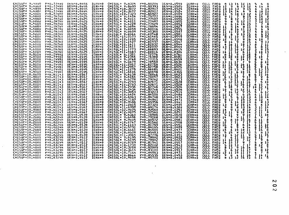
(.fi l S!JP '},'HJOO P o,/74dO lltN=O,On'iS lU?H 0 CHISUL= 9,1i37n 1"=0,80204 CHI SIJP 9,4ouo P O,Tf4tl0 l!EN=0,06'i5 li:.Rk 0 CHISQL= '1,8o"'9 P=0,6039J CH 1 SfH' 9,4000 p 0,714110 U~N=O,ObS'i li:.RH 0 CHISQL=10,3072 P=0,82Rp CHIS!JP 9,1t()01l p 0,7/4tl(J llf:N=O,OI'>'i'i JI:.Pk 0 CHISQL•10,3072 P=0,82R 1 CH1SQP 9,4000 p 0,7/41l(l lHcl'l= 0, 0655 fEPk & CHlSOL::10,7J23 P=0,84927 CHISQP 9,6000 p 0,7tl7b0 lit:.l'i=ll.fll>2!l I:.RH CHISOL= ':11,1404 P=0.75727 CHJSQP 9,6000 P O,ltHt>O l!fi'I=O,Ob2~ li:.RH 0 CHJSQL= 9,4011 P=0,17487 CHISQP 9,6000 P U0 /H7bO U~N=O.Ob25 I l:.f~l< o CHISQL= 9,40~1 P=O ,17487 CHI S1JP 9,~>ooo p 0,7tllb0 Uf.N=0,0625 IERH 0 CHISI~L= <,~,42 8 P=0,71629 CHI SclP 9ob000 P O,HHbiJ 1JlN=O.Ob2!> li:.RH 0 CHISQL= 9,!1b94 P=u,·ra694 CHI SUP ~.6000 p o. 711"160 l!ti'I=0.0625 li:.UR 0 CHISQL= 9.11059 P==O.B0016 CHI SOP 9.6000 P o,/M/60 LiH<::0,0625 11:.Rfl 0 CHISQL= 9,11609 P=0,80340 CHI SUP 'J,l'>OOO P 0,7tHoO Ui:.N=O,Ob25 p:Pk 0 CHfSQL= 9,6964 P=o.ay548 CftlSQP 9.1:>000 P 0.71H6U l!i:.N=o,oo25 I:Rk 0 CH SQL=10o0~7:\ P=o.8 4t-5 CHI SUP ':1,6000 I' o.7117t>O (JI:t-1=0.0625 JERk 0 CHISOL=l0ol205 P=0,81815 CHIS riP 'l,bOOU P o,7117bU UE.N=0.0625 llRH 0 CHISQL=10,1427 P=0.81937 CHfSflP 9,6000 p 0,7il7b0 lJlN=O,Ob25 fi:.RH 0 CHfSQL=lO•fbll P=0.620n CH Sill' 9,6000 P o.7tHoo Ut.t-~=Oo0b25 I:.RH 0 CH SQL= Oo b P=0,820 CHI Sr~P 9.6000 P o,78l6o Ut.N=0,0625 li:.Rk 0 CHI SQL = llo 117 3 P•0,86893 CHJSQP 9,6000 P O, liHbO Ol:ti=O,Ot>25 II:.Rk 0 CH1<;QL=llo4S83 P=o.8aou, CHfSQP 9,8000 p 0,7'1'Hil Ot::N=0,059S fERH 0 CHfSQLa 8o7351 P=0,72J76 CH SOP <~.11000 P 0,7'i<W Liti'I=O,OS95 t:RR 0 CH SOL= 9,2354 P=0,76 80 CHI S11P 9,8000 p 0,19981 lJI:.N=O,O!:i95 li:.RR 0 CHISQLo: 9.3748 P=0,17315 CHI SUP 9,~000 P o,799!l1 Ut:U=0,0595 llRR 0 CHISOL= 9o5b79 P=0.78559 CHISQP 9,Aooo P o, 7~9tH P,EN=0.0595 llRR 0 CHfSQL=ts•29St ~=g.82J58 CH SllP 9,Aooo P o.79~bl u~=o. os'is ERR 0 CH SQL= ,295 •• 82 58 CH1SnP <J.eooo P O, 19<Hll l!tN=0,0595 1EPR 0 CHISQL=llo1275 P:o0,86685 CHlSQP ':ll,f!OOO P 0,19'lH1 OtN=0,0595 II:.RR 0 CH1SQL=11,6•04 P=0,88698 CHlS!H' 10,0000 P u.BlJ'tJ UlN=0,0567 lERH 0 CHJSilL= 9o6p8 P•O,J884~ CH1S<W 10.0000 P o.ul 43 Lii:.N"'O.OS67 llRR U CH SQL= 9of> 54 P=o. sa5· CH15!JP 10,0000 P Uotlll43 lJEN=0.0!,67 II: PH 0 CHISt}L= 9,6178 1-'=0.79242 CHlSQP 10,0000 P (J,IH14] IJUI=O,OSb7 IERH 0 CHlSQL=10o2793 P•0,8?67l CHISOP 10,0000 p 0,111}'*3 lJI:.ti=0.0567 ftRR 0 CHfSQL=t0,2793 P=0,8~671 CH1S!W 10.000'1 P O,H1 43 Ut:N=0.0567 RH 0 CH SQL= Oo2931> P=0,8 74 CHIS<JP 10,0000 P O,t!1J43 lJEN=0,0567 lERR 0 CHlSQL=f0.2'736 P=0,82746 CHlStlP IU,OUOO P O,bl 43 UEN=0.0567 lfRH 0 CHISOL= 0,3853 P=0,83223 CHlSrlP 10.0000 P O,IHI43 Of.N=0,0567 lE.RR 0 .CHISQL=10o6424 P=0,84500 CHlSilP 10,0000 ... 0,81143 lJI:N=0,0567 ltRR 0 CH1SQL=10o6943 P:0.84748 CIHSOP 10,1)(}00 P o.IH143 Ull~=0,(1567 li:.HR 0 CHISilL=10o1182 P=Oo84861 CHJSrW 10,0000 p 0,81143 lJf_N::0,05b7 li:.RR 0 CHlSOL=l0,9!:>86 P•0.859'56 CHJS1~P 111,0000 P u.B1143 lJti'I=0.0!:)67 JERH 0 CHJSQL=llo2815 P=0,81320 uusnr 1o.uouo P Oo81143 l!I:N=O.O!:>b7 ~-RR 0 CH SQl=llo4'J9A p:;;Q,88l74 Clt1SQP 10,0000 p tl,ttll43 Utt-1=0.051'>7 II:.RR 0 CHISOL=t2,9075 P=0,92560 CHISQP IOoOOOO p tl,tl1143 LJI:.N=0,0567 lt..RR 0 CHlSQL= 2o9075 P=0,925b0 CHlSQP 10.~000 p 0,!12;>48 U~N=O.O!'i39 flHR 0 CHfSOL= 9,6360 P•0.78985 CH ~f}P 10.2000 P O,ti224b Uf.I'I=O, 0!;39 1:.1'!11 0 CH SQL= 'J,b496 P=0,79068 CIHS!W 10oc000 p tJ. ~2?4t< IJlN=O.tl!:)39 li:.RH 0 CHJSOL= 9,9005 P=0,80572 CH1SilP 10,2000 P o.tl224ts Oll'l=il.0539 lERH 0 CHISQL=10,0747 P==0,81562 CHlS!JP 10,?000 .., o,!lC:?4b UlN=0,0539 JERR 0 CHISOL=l0ol~03 ~=0.81J59 CH S!)P 10,?.tJIIO P Uoli224h lJf_N=0.0539 lRk 0 CHISI~L=lUo5 31 =0,84 65 CHlSQP 10,?UOO P u.u~?.411 UtN=0,0539 li:.RR 0 CH1SfJL=J0,6641 P=0,84604 Cli}SIW )ll,i:'OOO P o.Mc24& L>~N=o.o539 H.RR 0 CHISQL=10.tl!:>2A P=0,85483 Ctt 1 S!~P 10.2UUll P o.&22'•1:l UlN=O,O!l39 llRR 0 CHJS!lL=ll. 3965 P=0,87176 CHlSQP 10o40IJU p 0,1:132':111:1 llHI=O,!I!:)12 li:.RR 0 CH SOL= 9,6195 P=0,78882 CHISM' 10,4000 P o,aJc<Ju Ut:N=0,0':>12 li:P.R 0 CHISQl-= 9,6195 P=0,78Rfl2 CHIS!H' 10.4000 P O,t!J2<J8 llt:.t-1=0,0512 IERR 0 CftiSQL=lU,0"/09 P=0.8154l CHIS!IP 10.4000 p n,H32'il:l OtN=o.ostz II:.Rk 0 CH1SQ~=10o1730 P=0,82102 CHlSQP 0,4000 P O,HJt9k lJtr4=0. 05 2 li:HH 0 c~uso =10.32os P=0,82Rfl9 Clll<;r~P }0,'•000 P O,BJi911 OI:N=o.o512 llRk 0 CH1SOL=10o3bl't P=0,83100 CHlSliP 10,4000 P !l 0 11J2Yb Ul:.ll=0,051?. 1lRH 0 CHISI~L=10, 71t;6 P=ll,tl4853 CttlSilP 10,4000 ~ O,IJ32':1H UI:N=0,0512 lEAR 0 CHISOL=tO,Ii644 P=O,II5535 LHlSclP !U,4000 t-' O.IIJi~tl UH4=0,05 2 llRR 0 CIHSQL= o.9008 P=O,II5700

llt.N=0,059o lERR=O Ot:.N:::o,oses IERR=O Dt:.N=o.o524 JERR=O OE.N•0,0524 lERR=O l>f.N::0,0469 ffRR=O OI:.N=0,0696 RH=O IJI:.N=0,0655 fERR=O OI:.N=0,0655 ERR=O OI:.N=o,065~ ltRH=O OlN=o.o62 I RR=o DI:.N=0,0595 p::RR=O VI:.N=0,0587 ERR=O ot:.N:oo,o5a~ JER~•O OI:.N=0,05'i E::R zo [ltN=o.osc;o IERR=O OI:.N=0,0547 IERR•O UEN=0,0544 fERR=O OI:.N=0,054tt ERR::O UlN=O • Oltl5 IERR:O OEN=0,0384 lERR•O BI:.N=0.0761 flRR=O t.N=0,068 I:.RR=O OlN=0,0659 IERR•O l>lNc:0.0630 IERR•O gE.N•o.o~26 I£RR=O tN=o.o 26 RR•O OI:.N=0.042l f.RR=O OI:.N•0,0365 lERR=O B~N=0.06~3 {tRR=o N=o.o6 3 RRzO OlN•0,06l3 IERR::O OEN=0,0528 1ERRao l>EN=0.0528 URR=o DI:.N=o.o526 RR:o OtN=Oo0526 lERH=O UlN=0.0514 IERR=O OtN=0,0480 lERR=O OI:.N=0,0474 IERR=O OtN=0,047l IERR=O OlN•0,044 lt::RR•O DEN=0,0404 JER~=O OI:.N=0,03RO ERH::O utN=o.ozsl fERR=O Ot::N=Oo025 EPR=O Ot:..N•o.o62o fERR=O IJI:.N=Oo0618 ERR=O OEN=0.0581 IERR=O OI:.N=U,O'i56 IERR=O oe.N=o.o~u IERR=o OE::N•o.o ERR=O l>t.N=0,0477 IERR•O (Jt:N=0,0454 IERR=O OEN=0.039~ fERR=O IJI:.N=0,062 ERR=O DEN=0,0622 IERH=O DlN=OoOS57 lt::Rfh:O OE:..N=o.o~4~ fERR=O OE.N=o.o 2 ERR=O OlN=0,0517 IE.RR=O IJEN:u, 0471 1ERR=O OI:.N=0.0453 OI:.N=0,0448 IERR=O

ERR=O

CELL FREQ 8 13 14 1l 14 s b s CELL fHEQ 10 9 8 13 12 4 16 8 CELL fREQ tO 10 f3 ~ 14 6 4 14 CELL fHEQ 3 14 4 4 9 6 10 0 CE~L fREQ 14 5 10 13 12 4 F 1o CE L fHEQ 9 11 1 8 15 6 6 8 CELL fHEQ 9 8 12 7 17 5 10 12 CELL fREQ 9 8 5 12 17 7 12 10 CE~~ FREQ 9 6 14 14 ~5 7 7 8 CE FREQ 11 5 14 8 1 7 8 16 CEL~ fREQ 12 8 16 11 13 5 6 9 CEL fHEQ 11 11 10 8 7 4 8 11 C L FREQ 12 9 13 6 6 C~l~ FHEQ 8 1t 10 8 ~~ 4 9 5 CELL fREQ 12 9 13 9 16 4 10 7 CELL FHEQ 8 14 9 8 15 4 9 13

g~t~ f~~g 1~ 16 JA 1¥ I~ 2 ~ 11 CELL FREQ 7 ~ 10 12 12 3 9 CELL FHEQ 14 11 12 6 11 3 10 13

E~t~ ru~g 18 a 11 13 IK ~ 1~ ' CELL FHEQ 9 9 ~ 1~ 7 8 9 5 CELL FREQ 13 11 17 1 9 5 8 10

~~~~ ~~rs tt 1~ lg ~~ tA ~ ~ tl CELL FHEQ ~ 0 13 9 13 5 fl CELL fREQ 12 13 6 10 14 3 2 10 CE~~ ~R~Q 15 7 ~~ ' ' 6 10 16 CE -H Q 6 13 1 8 9 6 CELL fREQ 15 9 fl 6 16 0 9 6 CELL FREQ 6 12 J 12 16 7 5 10

~E~~ f~~g ~ lA 1 ~ 1 t~ 1~ l~ 1f CEL~ FREQ 1~ 9 10 12 11 4 17 CEL FREQ 14 12 9 15 5 b 12 CELL FREQ 12 13 5 6 ~5 6 11 12 CELL FREQ 13 5 6 13 3 6 10 14 CELL FREQ 8 1~ 1 15 13 8 12 4 CELL fREQ 9 14 13 13 6 8 13 CELL fHEQ 13 9 12 10 ~4 5 4 l3 CELL FREQ 9 8 8 3 4 3 11 4 CEL~ FREQ ~4 9 13 8 12 2 ff 11 CEL fREO 3 11 9 12 14 2 c~t~ fHEQ 5 1J 9 9 lo 1 11 17 C REO 14 9 ~~ 1 6 9 CELL FREQ 6 8 10 - 16 6 11 8 CELL FREQ 12 7 13 7 17 5 12 9 CE~~ fR~Q 16 ~ 6 14 6 IJ l~ CE R Q 8 4 4 8 2 CELL fREQ 14 4 10 10 11 7 6 8 CELL ~REO 5 15 9 12 13 5 8 13 CE~~ REO 1~ 4 12 ~~ 9 5 ~~ 11 CE REQ 6 1 18 9 CELL fHEO 11 18 10 7 12 7 9 6 CELL FREQ 14 10 17 9 1 5 8 10 EEL~ FREQ 5 13 13 I 11 ~ 12 8 EL FHEQ 8 1 9 16 4 8 7 CELL FREQ 5 6 12 11 17 9 8 12 CELL FREQ 12 11 10 1 17 4 7 8 Cl::ll ~REQ CELL HEQ ~ 13 1~ u it l It 1 ~

"' 0 N

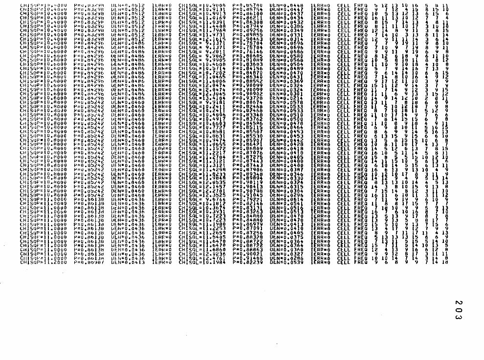
LHI Sllf' CHI Sill' CHlStW CHI SeW CHISrlP CHLS<W CHISQP CIHS<ll-, CHISQP UllS<W tHISrlP c~' 1 srw (;H 1 :)r)P CHIStW ltll SOP (.ttl SliP CHI SOP CHiSQP CH 1 sr1P Ctll'>oP CHJSIIP CHI SliP CHI SUP CIHSQP CttlS<lP CHlS•.lP Lti[S()P CHJSQP Ctll StiP UHStlP CIH SIJP CHI StlP CH1S()P CH 1 S·ClP CH[Si1P CtllS<lP CHI S!lf' Ctll SliP Clll SllP CHlSQP CHfSQP Ctl S<H' nusrw CHI SrlP Ctll Srlf' CH1Sr1P CHlStW CHISilP Ct!fSOP C:H SliP (;H l S•IP CHISQP CHI srw CtHSilP CtHSYP CH 1 Sill-' CHISQP Ct!ISIH' CiHSQP CHISQP CHISf)f' CH1S<lP

1 o •. ·.oou I0.40Ull 10.4000 10.4000

l0. 1t000 0.4000

10.4000 10.4000 10.4000 10. r>ooo 10.6000 IO.oooo 10.6000 }O.f>OOO lO.bOOO 10.6000

10.6000 o.Auou

1o.,,ooo 10.6000 10.6000 10obOU0 10.6000 10.ROOO lO.IlOOO 10.!!000 10.AOOU 10.ROOO 10.8000 10ollOOO 10.1l000 10.Il000 10.8000 10.HOOO 1o.nuoo 10.1lOOO 10.11000 1U.HOOO 10.13000 1o.uooo JO.IlOOO IO.HOOO 1U.H000 10.1J000 lOoflOtJO 10.Rooo 11.0000 u.oouo u.oooo u.oouo 11.0000 11.ooou n.oouo u.oouu 11.0000 11.0000 11.0000 11.oooo u.oooo 11.0000 11.0000 11.2000

p o.cUr''~f1 P o.tuc:•Je P o.tn~<:~li p il.td2':1b p o.tU1.91< P o.tJJ~9u P o.eJt><tu P O.bJI.'ltl P o.e3c98 P o.l!42'llb p 0.842':11> p ll.l1'+2'lb P O.tl'+2'l6 P o.tHc':lb P o.l!'+29t> P o.tl'+c'>'b P o.l:l42'ft> p !t.tl'+2'lh P o.U429b p 0.!14<'96 P o.ll429o P o.u429o P Ootl4c'lb P o.tl~c42 p 0.1!::.242 p 0.1!~242 p IJ 0 ti!JC'42 P o.!l~c42 P o.tl::.242 P u.ll~24i.' p 0 .tl~242 p 0.!!~242 P O.tl~i:''t2 p 0.!1~242 P o.l!~c42 p o.u::.~42 P o.tJ::.242 P u.tl~242 p 0.11~242 P u.8~242 P o.l!~2'+c P o.H~242 P O.H~i:'42 p 0.!!~242 P o.u~~42 P o.e~c42 p 0.8bl38 P 0.1Hll31! p 0.86138 P o.tJ6 31! P O.tlblJtl p 0 .l:lbl3tl p o.uol3ts P o.B6l3tJ P O.lli:>l:HI P o.Hol3& p o.uof31i P O.Hb JH P 0.6ol3H P (I.B613U P o.uo131'1 P llotlb'Jtl/

uu,"n.o!:l1c IJUl=O.O!Jl2 ut:N=o.n512 L.tt.N=O.O!J12 l.li:JI'"'0o0512 1Jtti=0.0512 UtN=Oo0!':112 UtN=0.0512 UE.N=0.0512 L.tt.N=0.0486 IJtN=O • 048(, IJtN=0.0486 Ut!~=Oo041:l6 UEN=Oo0'+!l6 IJI:.t~= 0. 0486 tJE:.r.=o.o486 IJEN=0.0486 UI::.N::Oo04B6 1Jf.N=0.0'+86 IJlN=IJ.O'+Bb Of_ N= 0 • 048b IJE.N=0.04Hii Ut:.N=0.0486 UlN=0.0460 UE.N=0.0460 IJf:.N=O • 0460 ULN=0.0460 UlN=Oo0460 L1E.N=O • 0460 IJtN=Oo0'+60 OlN=Oo0460 llt::N=0.0460 IJE.N=Oo0460 UlN=0.0460 llE:.tJ=o.o460 lJEII=0.0460 Dt:N=0.0460 Ut.N=0.0'+60 UFN=0.0460 IJI:.N=0.0460 OlN,.,0.0460 O£N=Oo0460 PE.N=Oo0'+60 OE.N=0.0460 Dt:N=0.0460 ut.r~=o. 0460 IJHI=Oo0436 OtN=0.0436 LJt:N=0.0436 llc.N=O • 0436 lJt:.N=0.0436 IJ[N=0.0436 Ot:N=0.0436 IJE.I•=0.0436 UEN=0.0'+36 Oli~=0.0'+36 llt'.tl=O • 04 "16 lJI:.N=0.0436 llf.N=0.0436 lH:N=u.0436 IJH•=Oo04]6 IJI:.N=O o 0'+13

lt.HH=O llRk=O It:lm=o li:.PR::O

l i:.Pk=U H<H=O

IU<H=O lE.RH=O I~PI<=O 11:.1<1•=0 1lRR=O llPR=O

l lRR=O I::.RR=O

IE.Rf<=O lf.RR=O

l l:.Ril=U I:.RR=O

ll:.RP=O 1lRR=O IlRR=O IE.RR=O llRR=O

II:.Rk=O E.PR=O lRH=O

lt: Rl\=0 lE.PfJ:O

IEPR=O tHH=O

IERH=O IE.PH=O

IE.RR=O I:::HR=O

llflH:;O IERH=O

l l:PH=O I:.HH=U

llRFI=O IEnR=O

IE.RH=g lPR= tRH=O

IE.RR=O IE.HR=O ll:.PR=O IERFI=O ltFIR=O

IE.RH=O tRk=O

IE.PH=O ~PR:O

IERR=O I:'.RH=O

li:.RP=O li:.FIH=O

l t:.Fik=O tPfl=O

lEPH=O llPf<=O

IE.RH=O tP.H:;O

CHfSOL=to.9UOA Cll SI)L= Oo9i31 CHISOL=10.9913 CIHSQL=ll.0169 CHISflL=tt•OJ91 CHlS!~L= o440A CH1SilL=11.1969 CHI SOL= llo 9731 CHJSOL=12o16l"i Cli S!K= 9.1J7\ CUISOL= 9ol371 CHISQL= 9.~011 CHfSGL= 9.906? CH SOL= 9.9905 CHISilL=l0o4bOO c•nsoL=10.!:iH4 CHISQL=t0.7202 CHl<;QL= la046S CH1SQL=llob006 CHJS<~L=l2o0474 CHJSGL=12oO<t74 CH1SQL=12.3045 CHISQL=l3.4l04 CHISOl= 9.9181 CHISQl=f0,241l CH S<~l= Oo24J CHISQL=10.4096 CH1SQl=10o4917 CtifSGL=f0o6603 CH SGJl= 0.7127 CHISGJL=10.8:0,81 CHISQL=l0o863l CHfSQL=lOo9474 CH SQL= lo06S5 CtHSOL=llol572 CHISQL=llo2217 CHISQl=tt·2J04 CH Sf)L:. • 3 21 CHISQL=1lo3121 CHISQL=llo429A

E~nat:H:S~H CH1SQL=l2.0!J35 CHISQL=12o1457 CHISQL=l2t270l CHISOL=l2oJ!:i25 CHISQL= 9o6144 CHJSQl=10ol812

~~nat=t8:3~H CHJSQl=lOo "1223 CH1SOL=10o1ic!23 CHfSQl=t1o1'180 CH SQL= 1.2253 CHISQL=11.2659 CHISilL=11.5405 CHf5fJL=tt•&470 CH SQL" o6470 CHJSQL=l1.6860 CHJSOL=l2o0236 CHfSQL=f2•4-161 CH SQL= o.l'i8

P=O.!l5700 P=0.857<;4 f>;:O.!l6100 P:0.86211 P=0,86308 P:;:O.!l7\)49 P=0.69256 P=0.69A55 p:g.90463 P= .75704 P:o.75704 P=Oo16146 p:0.80605 P=Oo8l089 P:0.83603 P=0.84156

. f>=Oo84A70 P=O.d6340 P=Oo8A5<;2 P=0.90099 p:0.90099 f-':;:0.90902 P=0,93728 p:o.ao674 P=0.82468 P:;0.82468 P=0.83348 P=0.837(>2 P=Oo845~6 Pao.asus P=0.85507 P=0.855JO P=Oo8590{ P=0.864?. P=Oo66809 P=0.87076 P=0,87275 p.::0.8744l P=0 0 87443 P=O,H7906

~~8:KU32 P=0.901l9 Pa0.904 3 P=Oo90798 P=0.91045 P=0.79221 P=0.82146 ~:8:3UU P=Oo84AAO P•0.848RO P=0,66979 P=0.87091 P=Oo872S6 P=0.8A3?8 P=Oo8R722 P=0.88722 P=0.88863 P=0.9002l P=0.91405 P=0.82239

OlN=Oo044B llt:.t~=0.0447 Dt.N=0.0437 UE.N,.0 0 0434 DE.N=0.0432 OtN:o.038& Dt:.N=0.0349 IJlN"'O • Ol31 OlN=0.0314 OEN:o.o696 Ot..N::0,0696 OlN=0.0686 UI:.N=o.osso OI:.N=o.o568 Of.N=Oo050it OE.1'4=0o04A9 DE.N=Oo0470 OE.N=0.0431 DlN=0.0369 Uf.N=0.0324 UEN=Oo0324 Ut.N=0.0301 DI:.N=0.0214 DtN=o.o578 OE.N=Oo0533 OEN=0.0533 OfN•0.05lO OlN=o.osoo Df.N=0,0478 DEN=0.0464 DEN::0.0453 Uf.N=0.0453 DlN=0.0442 UI:.N::o,0428 OlN=Oo04~8 OI:.N•0.04 0 DEN=O,OitOS Ot:.N=o.o4oo OEN•Oo0400 OEN=0.03!!7 Of.N=0.0346 OEN=Oo0330 OEN=0.03?.4 Ot.N=0.0315 OI:.N=Oo0304 0tN=0.0296 OlN=0,0614 Ut:.N=0.0541 Et~:8:8~U OI:.N=0.0410 DlN"'0o0470 OEN=0,0413 Uf.N=O,Oit 0 DE.N=0 0 0405 OI:.N=o.o375 DEN=Uo0364 OEN=0.0364 OEN=0.031'10 OEN=o.0327 UE.N= 8 • 8 ~86 Ot:.N= • 539

1lRH=O

IERR=O E.RR=O

lt::RR=O

IERR:O t:.RR=O

lE.RR:O 1ERR=O

IERR=O ERR=O

lERR::O IE~R=O

IERR=O EHR•O

lERR=O IERRo:O

IERR=O ERR:zO ERR=O

IERR•O IERR=O IERR=O

IERR=O ERR=O ERR=O I::RR=O

IERR=O ERR•O

RR=O ~RRao lfRR=O lERR=O

IERR=O ERR=O

IERR=O IERR=O

u~~=s IERR=O IERR•O u=n:s IERR=O IlRR=O IERR=O IERR"'O

IERR=O ERR•O

IERR=O ERR=O

IERR=O ERR=O

IERR=O ERR=O

IERR=O lERR=O u~~:s lERR=O lERR=O

IERR=O ERR so

CELL FRFQ ~ 12 ll lO 16 5 b 11 CELL fRfQ 9 1 12 4 15 8 15 10 CELL FHEQ 10 5 13 12 13 6 15 6 CELL fREQ 16 11 13 10 12 1 7 4 cELL FREQ 8 ls I fit lJ 4 a 1• CELL FREY H 1 I 0 1 3 1U 0 CELL fHEQ !2 14 8 ~ 11 3 8 15 CELL fREQ 7 14 10 3 13 8 11 14 CEll FREQ 12 9 11 11 14 3 6 14 CELl FREQ 7 7 9 9 11 9 8 0 CELL fHEQ 7 10 9 1 19 8 9 11 CELL FHEQ 9 9 11 9 19 6 9 8 CEtl fRfQ 8 12 6 l8 ~ 6 11 to CE L FHEQ 10 5 8 8 II 8 8 2 CElL FREQ 11 10 9 10 8 4 10 8 CELL FREQ 5 7 9 l~ 16 7 13 9 CElL fHEQ 9 6 14 fit 10 6 6 15 CELl FREQ 1 14 8 0 6 4 9 12 CEll fHEQ 9 17 12 11 10 3 9 9 CELl FREQ 15 11 12 9 14 3 1 9 CEtl fREQ tl I 14 9 12 3 9 15 CE l FREQ 1 6 9 3 3 15 2 CELl FREQ 14 14 12 10 2 8 11 CELL FREQ 13 1~ 1 a 18 6 8 9

E FREQ 1 0 12 18 1 9 8 gt:tt FREQ 1a lo 18 11 5 12 9

CELL FREQ 11 10 11 lit 9 1 6 6 CELL FREQ 1 8 14 15 15 6 7 8 CELL FFREQ 11 10 8 9 f8 4 9 11 CELL REQ 6 9 8 10 1 5 16 5 CELL fREQ 8 6 9 -g 14 5 16 13 CELL fREQ 6 13 15 ~ 15 6 6 10

~~tt ~~~2 l~ i.1f ~~ l~ 12 1~ 9 CELL fREQ 14 5 12 6 13 7 8 15 CELL FREQ 16 10 5 11 lit 5 8 11 ~~tt ~~~g ~~ y 1~ 1~ 1 ~ •g ~~ 1g CEll fREQ 6 lo 14 5 15 6 13 11 CELL fREQ 16 6 13 9 ll 10 4 9

~~tt ~~~g 12 ~~ 13 11 * g ~~ 1: CEll FREQ 8 13 13 10 14 4 5 13 CELL fHEQ 14 3 8 10 15 9 13 8 CEll FREQ 1 15 14 8 12 3 ll 10 CElL FREQ 16 11 6 10 11 3 12 CEll FREQ 7 11 9 19 9 6 10 9 CELL fREQ 11 B 8 17 15 7 7 1 CELL fRf.Q 18 10 9 9 5 9 13 CELL FREQ 1 7 6 10 16 8 7 0 CELL fREQ fl 5 f3 ·v 11 8 1 8 CEll FREQ 3 9 3 5 !l 8 17 7 CElL FREQ l5 5 10 9 13 7 15 6 CELL FREQ 3 4 1 9 12 1 9 9 CELl FREQ 8 9 1 11 17 11 4 13 CELL fREQ 5 13 13 13 15 6 6 9 Cl::lL fREQ 7 13 ll 5 l5 5 f4 10 CELL FREQ 15 1 5 4 10 3 5 CELL FREQ 12 4 13 9 16 6 12 8 CELL FREQ 9 9 12 8 17 3 11 11 CElL FRfQ 10 10 14 7 14 3 lit 8 CELL FREQ 9 6 8 9 9 7 4 18

"' 0 w

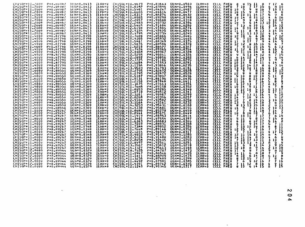
(;fll';flf'=JI.?OOO CH!StlP=ll.2UOO CtilS!lP=ll.20UO CHlSQP=ll.?.OUO CHJStH'=ll.20UU CHJSQP=ll.?.UOil CtilSOP=ll.?.OOO CHISrW:::JJ.cOUIJ CHISUP=llo21l00 CHlS<lP=I I .21100 CIHSIH'=ll.?OOU CHJSQP=tl.2000 CHJSQP=ll.4001i CltJSrH'=ll.4000 CH1SUP=1l.40UO UUSfiP=1lo4000 CIHSQP=l t o4000 CHISQP=l .4000 LHlSr.!P=11.4000 CH1SQP=1lo't000 CHfS•H'=J l•'•OOO CH <;r)P:::J .4000 CH1S<JP=ll.4000 CHJSQP=11.4000 CH1SilP=lf•4UOO ClfJSQP=i .6000 C:HISflP=llo6(lOO CHlSi~I>=Jl.6000 CHJSQP=ll.6000 CHISOP=ll.6000 CHISQP=Jl.6000 CHJS<lP=llof>OOO CHISQP=11.6000 CtilSllP=ll.nOOO CIHSrJP=llof>UOO CHlSilP=Jl.f>OOO CHlS!H'=ll•6000 CHlSIJP=l .t:-000 CHIS<H'=11.600U CHJSQP=llohUOO ClllS<JP:tJ.llOOO CHJSQP=tl.HOOO CHlStH'=ll.AUOO CtHSUP= 1l.t1000 CHIS<H'=Jl.HOOO CHIS•lP=Jl.HOOO tHISQP=ll.HOOO CIHSQP=llol:\000 (.HJSQP=ll.liOOO CHlSOP=ll.I:IOOO U!lSflP=lloAOOU CHJSQP=11.1100U LIHSrH':::- 11oHOOU CH1SQP:::Jl.H000 CH1S<H'=11oH000 CHISrW=l2.oooo CH1SrlP=12.oooo CHlSoP:J<>.oooo tt1l S<lP= 12 • 0 0 0 0 CHisrJP=J2.oooo CHJSrlP=l2. 0000 CHJSQP=l2.0000

P=O.UO'ol/:1' P=O.Ub~Hl P=O.btJ'iU7 P=U.ilb':lbl P=U.tlb':lbf P=U.tio'ilif P=O.IJo'JIIif P=O.Iio<ib.f f'=O.dt>':lt\7 P=U.tlo':IH/ P=O.Hb':ltl/ P=U.tlb':lb7 f.'=O.H/7'JU P=Uolif7':/U l'=o.H 17'10 f.'=0.0/7'10 P=O .IH 7'JU I'=Ootl77<JO P=O • 817<JO P=O.Iif7<JO f.'=0.~77<JO f.':Ooi:I77':1U P=O.I:I77':1U P=0.8F190 f.'::::O • 8 7.('10 P=0.8t15~0 P=O • 8tt!>!>O P=OoUtl!:>!:>ll P=O .1Hi!:>50 P=O • !Hl!>!:>lt f.'=0.81:1b!:>O P=0.8tl!>~O P=O.dt!!:>!>O P=0.8b!:>!:>O P=0.8t!!:>!:>O P:O.i:IU!:>!:>O P:O.Iltl!l5U P=U.tlt1!:>50 P=O.tlti!:>!:>O fl::::O.Hb550 P=Oot1':12bl P=o.8':1<?t>7 P:O.Il':lcl:l7 P=O • fl':llt:>T P=0.8'1267 P=o.a'>'cl:l7 P=O.t!9267 P=0.8':1261 P=O.t1':1267 P=O • tl'Jlb 7 P=O.d':l267 P=O.tl':/21:!7 P=U.Ii'J2b7 P=O.I:I':I.?b7 P=O.I:l'J2b7 P=O.H':I':/44 P=Ool:l'l944 P=ll.B'1<,144 1>=0.11'7944 P=Ool:l':1944 P=O.tJ':I944 P=O.tl':1':144

1!!-t·t;:;0.0413 lllll=ll.04l3 IJI.N=II.04}3 UUl=Uo0413 lll N=0.0413 U~ll='Oo0413 IJlN=0.0413 UlN=0.0413 lJI:.N=Oo0413 UU<=0.0413 IJ[N:n.Ottl3 U~I~==0.0413 Ut.u=o.o:wo lJI:.N=Oo03'JO UtN:O.OJ':IO ut:.N;:o.o39D Llltl==O • 0390 ut.t~=o. 0390 lJt:.N:0.03':10 lJt.N=Oo0390 Ut:N:O.OJ90 lJI:N=0.0390 lJHt=0.03':10 UtN=0.0390 lJHI=O. 0390 IJI:N=O.OJ69 lJt.N=O • 0 3t>9 1Jt.N:0.0369 1Jt-.N=0.0369 UtN=O.OJ69 IJI:.N=0.0369 Ulll=O.OJ6<J lJUl=O • 0369 U(N=0.0369 IJEN=0.0369 UI:.N==0.0369 lli:.N=0.0369 IJI:.N=0.0369 IJEN=0.0369 Ot.N==0.0369 UE.N=0.0348 Ol:.l't=O • 0348 llt.N=o. o ::148 OUI=0.0348 OEN"'0o0341l I.JI:.N=0.0348 LJF.Il=O. 0348 UlN=0.0348 Ut:.N=Oo0348 LJt:N=o. o:-t48 0tN=0.0348 I.Ji:N=O.OJ48 IJI:.N"'Ilo0348 IJI:.N=0.0348 Ut.N=0.0348 UI:.N"'0o032<J lJI:.N=O.OJ29 UI:.N=OoO.l£'9 IJI:.N"'0•0329 Ui:.N=0.0329 I.Jf-.N=O.OJ29 IJI:.N:.0.0329

(I:.R~=U 11:.k~=O ll:.llk=O lt.PJi=O IU<k=O lUHl=U li:.Rt<=O llRil"'O H.RH:O llRH=O li:.RJ<:O 11:.111-1=0 ll!<H=O li:.RH=O li:.RH=O li:.PH=O

l lRR=O t:.RH=O

li:.I<R=O H.RH=O

II:RR=O lPH=O

IE.Rk=O li:RH=O

IEIW=O t:.RR=O

IERH=O lt::Rk=J

II:RR=O E.Rk"'O

IERt-<=0 lf.IHt:oO lERH=O lf.Rk"'O II:.RA=CI li:.RR=O lERH=O li:.RH=O li:.RH=O lERR"'O

l f.RH=O I:RH=O

llPk=O lEPH=O

li:.RR=O I:PH=O

II:.RH=O li:.RR=O li:.RH=O li:.Rf!=O llRR=O 11:RR=O

II:.RR=O lRH=O

li:.RH=O li:.RH=O li:.RH=O lERH=O IERH=-0 li:RR=O li:.RH=O ii:Pk=O

CHlSflL=lU.'+b7Q CHI'lf~L=lO.SlA? CHISOL=l0.5'10l CHISOL=10.6665 CHJSQL:1l.0312 CHISQL=ll.t1065 CHIS<JL=l2.2057 CH1SOL=12.2483 CH1Slll=1;!o5465 CHISOL=12.6190 Clil SOL= 12. 9J35 CHISIJL=12.1J795 CHfSOL"'lO.fb20 Cll SllL=10.':1J05 CHISilL=ll.!>461 CltlSilL=11.5b76 CHISQL=1t·6210 CHISIJL:1 .1'+2i> CHl SfJL=l2o 0068 CH1Sill=12.0295 CHISQL=f2.2892 CHlSf.lL= 2.J725 CHISilL=l2.~c84 CHISUL=lJ.l15il CHfSQL=f3,9503 CH SIJL= 0.27<,~5 CHI Sfll=l 0 • 2795 CHJS(JL=l0.5l87 CHISQL=ll.0131 CH1Sill=l1.2150 CHISOL=11.Jo75 CHISnL=ll. -,biiA CHISQL=11.8053 CHISQL=11o87l 0 CHJSQL=12.3261 CHISQL=12.8268 CIHSilL=12. 1:H60 CHISUL"l3.1564 Clfl Sf.ll = 14 • 3253 CHISQL;14.4J30 CHfSQL=J0.6U80 CH SOL= 0.8944 CHISOL•11.1919 CIH SilL= 11.3401 CHISQL=ll.6363 CHISilL"'11.704Q CH1SilL"'ll•73AA CHISIJL= .7t>413 CHfSQL=l2.1216 CH SOL= 2.4802 CHISilL=J2,5024 CHISUL=12.8458 CHJsQL=l2.tl997 CHISQL= 3.3567 CH 1 SOL= 14 .JJ27 CHJSilL=10.7025 CHlSQL"'1l•0947 CH SQL= 1 .ltlll CHISClL=11o3236 CH1SOL=11o4492 CHJSQL=11.9391 CH SQL=12.1240

1-'=0.63643 P=O.ti38Q4 P=0.64247 P=O.tl4616 p:o.tln274 P=O.tl9290 P=0.90600 P=0.9073l p;0.9f604 p:::o.9 sns P=0.92625 P•0.~273t, P=0.85066 P=O.HSR32 P=0.8R349 f'"'0o8R504 P=0,886?7 P=0.89065 P=0.89967 P=0.90041 P=0.90856 P=0.91104 P=0.91553 P=0.93066 P=0.94793 P=o.B2672 P=0.82672 P=0.83897 P=0.86195 P=O.II7049 P:::O.II76i>3 ..... 0.1!91511 P=0.8Q285 p .. o.tt9512 P=0.90967 P=0.92356 P=0.92582 P=o.93161 P=0,95431. P=0.95601 P=0,85279 P=0.85671 p .. o.ll6953 p:;0.87554 P=0.88683 P=0.88931 P=0.89052 P=0.89144 P=0.90337 P=0.91417 P=0.91480 p .. o.924o!J P=o.92541 P::0.93612 P"'0.95443 P=0.84787 P=0.86546 P=0.8fl909 p .. o.874A9 1-'=0.117981 P=0.89742 P:0.90345

UI:.N=o.uso3 UlN=0.0496 Ut::N=o.o487 UI:.N=O • 04 77 UI:.N=0.0432 Ut:.N=0.0348 UlN=0.0310 UI:.N:0.030b OI:.N=o,0280 ot::N=o.o271t 1Jt.N;0.0249 UI:N:o.0245 UI:.N=0,046~ UI:.N=0.0445 UlN=0.0375 DEN=0.0370

B~~:R:8~~z UI:.N=0.0328 OI:.N=0.0326 UI:.N"'0•0302 Lti:.N"'O • 0295 UlN=0,0281 OI:.N=0.0235

8EN"'0.0181 tN=o.o528

UlN=0.0528 OlN•0.0496 DlN:0.0435 UI:N=o.o411 Ut.N=o.0394 OEN"'o.oJ52 OI:.N=0.034H OlN=0.0341 UEN=0,0299 UEN=0.0257 Uf.N=0.0250 UI:.N=o.o232 IJI:.N=O.Ol60 Of.N=0.0155 U~N=0.0459

· OE.N=O • 0449 UI:.N=0.0414 OI:.NcO,Q397 DI:.N=o.o365 UI:.N=0.0358 OtN=0.0355 UI:.N=0.0352 OI:.N•O • 0 317 Ut:.N:o.o285 DI:.N:0.0283 OI:.N•0.0255 lJI:.N=0.0251 Ut:.N=o.o218 OE.N•0.0160 UtN=o.o47J OI:.N=0.0425 Ot.N=0.0415 DlN=0.0399 Ut:.N:0.031!5 UEN=0.0335

7 Ut.N:o.OJl

IERR=O II:.RR=O IERR=O IEPR=o li:.RR=O llRR=O li::RR=O lERRrO

IERR=O ERH=O

IERR=O IERR=O

IERR=O ERR=O

IERR=O IERR=O

IERR•O ERR~:o

IERR=O lERR=O

I""RR=O ~RR;O

IERR=O IERR=O

IERR=O ERR=O

IERR=O IERR=O

IERR=O ERR=O

IERHcO IERRaO

IERR=O ERR=O

IERR=O lERR=O IERR:O IERR=O IERP=O IERR•O

u~~=s lEHR=O IERR=O IERR=O IERR=O

IERR=O ERR=O

IERR=O ERR•O

lERR=O IERR=O JERRo:O JERR=O 1ERA=O IERR=O

II:.RR=O ERR=O

IERR=O lERR=O

IERR=O ERR=O

CfLL FHEQ 6 8 15 11 8 CELL fRfQ 1 10 1 17 15 CELL fREQ 10 5 9 II 18 CELL fHEQ 10 15 9 8 17 CELL fREQ 8 10 11 14 17 CELL FREQ lU 14 8 10 12 CELL fREQ 17 9 ~ 6 12 CELL fHEQ 10 9 5 14 13 CELL fREQ 7 13 It 10 f1 CELL fREQ 14 8 10 10 5 CELL FHEQ 11 11 8 6 13 CELL FHEQ 9 fl 13 13 12 CELL fREQ 12 0 6 6 f8 Cf.LL fHEO 9 7 10 6 6 CELL fHEQ 11 9 17 1 9 CELL fHEQ 12 12 II 16 14

8~t~ ~~~g li ~~ 1! ~~ ~~ CELL fREQ 9 11 14 16 8 CELL fHEQ 9 S 13 14 12

~~~~ ~~~g 1s ll 1 ~ tl ~~ CELL fHEQ 10 14 5 4 11 CELL fREQ 10 12 14 13 8 ~~~~ ~~~g 1~ 13 1¥ 1A ~~ CELL fHEQ 12 9 9 8 10 CELL fREQ 9 10 8 10 19 CELL ffREQ 1f 10 8 13 111 CELL REQ 1 16 9 7 16 CE.L FREQ 6 12 13 7 7 CEL~ FHF.Q 10 14 9 11 7 CELL ffHEQ 8 f2 10 5 tO CELL REQ 8 3 1 6 2 CELL fHEQ 13. 1 13 11 1o CELL fREQ 14 7 10 9 16 CELL ~HEQ 12 1 a 15 1s CELL fREQ 13 9 10 4 0 CELL FREQ 6 13 13 15 10 CELL fREQ 14 9 1 11 14

~~tt f~~g 1~ ' t3 lA 19 CELL fHEQ 1 10 11 1 11 CELl FHEQ 5 f1 9 8 17 CELL fREQ 6 0 6 12 17 CELL fREQ 6 f1 9 14 17 CELL fREQ 7 8 12 10 10 CELL fRfQ 12 15 5 ·7 16 CELL fREQ 7 1 13 9 f1 CELL fREQ 12 11 16 10 4 CELL FHEQ 14 f1 14 8 15 CELL FREQ 1 0 17 13 11 CELL fHEQ 15 13 13 It 13 CELL fREQ 13 6 9 11 4 CELL FHEQ 12 10 8 9 1o CELL FREQ 11 6 6 7 19 CELL FREQ 14 l1 6 8 l8 CELL FREQ 8 0 6 14 8 CELl fREQ 8 12 15 1 17 CELL fREQ 1 6 9 12 16 CELL FREQ 7 11 12 8 f6 CELL FREQ 8 0 b 14 5

1 11 b 6 8 10 7 10 13 5 8 u 5 9 6 4 6 16 3 10 12

10 15 4 3 16 12 7 3 13 3 14 14 4 14 4 9 1 12 6 10 b 4 14 9 5 6 7 5 6 13 6 16 5 4 12 6 5 , 15 9 4 14 3 9 9 4 14 8 6 3 14 g l g 1~ 6 1 19 5 11 8 5 8 7 5 8 8 6 12 7 4 1 8 5 13 l7 4 7 I 4 b 0 3 9 12 3 l(l 10 3 b 15 2 lj 11 2 10 13

l u l 7 6 15 7 15 8

~ 1~ ~~8 • 8 I 7 1 4 17 6 4 4 6 tl 3 10 9 8 5 9 3 9 15 2 13 10 9 tl 12 7 1 9 6 10 8 7 8 6 1 7 16

~ 1 ~~

N

0 ~

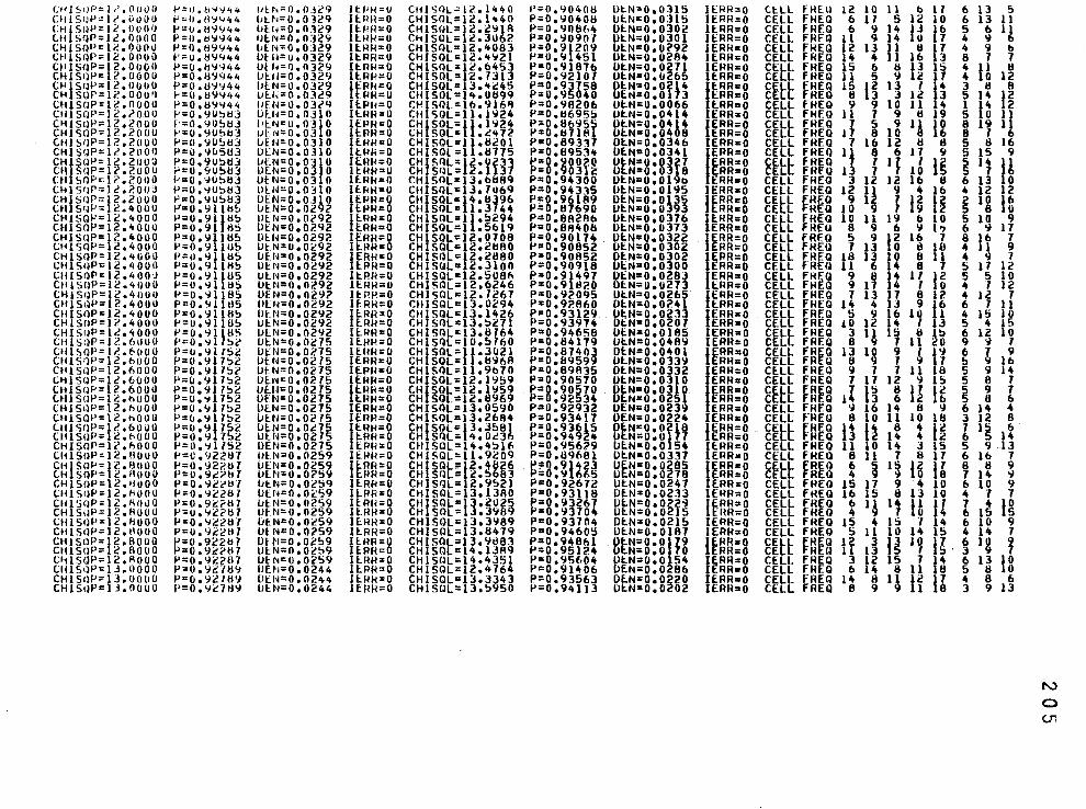
CHJSrJP lr',OOOO I-'=!J,b'-;'144 IH. ~.=o. OJ29 lt::l•fl:O CHI51lL=l2,1440 f'=0,9040tl Ut.N=0,0315 CHISrJf' ll'.ouoo f'=O,B'i'-144 IJt:.~•=O, 0 329 li:.HR=O CHIS<R=l<!,l440 P:;;0,9040B IJI:.N"0,0315 CHIStH' J£',0000 P=l!,ll':I'J44 IJH<=0.0329 flRR=O CHlSfJL=lc,clllR P=0,90B64 OI:.N=0,030c (.HlSijP 12,0(100 P=ll,tjll':/44 UI:.N=0,0329 I:.HRo:O CI11SOL:::l2.3062 P=0,\1090/ Ot.N=0,0301 Oil Sfll' \c. OOllll P=ll,1;3'i944 lli:.N=0,0329 li:.RH=O CH1SQL=12,4083 p:0,91209 OtN=o.o292 CHlSflP 12.0000 P=u ,I:I'JY44 U~ll=u.0329 li:.RR:::O CHISQL:::lco'+'l21 P=O,'H45l Ut.N:::o,o28'+ ClllSUP 12.0000 P=O,H':I944 u~ r•=!l,0329 It.RH=O CH1SOL=F'•b453 P=0,9187b Ot.N=0,0271 CHlSflP 1i',OOOO P=O,I:l':IY44 lJI:.Il=O, 0329 llR!J=O OHSQL= 2.7313 P=0,92107 OI:.N=0,0265 Cl-lfS<W 12,0000 P=O.tl':l944 lJlN=0.0329 fp~H=O CHISUL=13,4~45 P 01 0,9~~58 BI;.N=0.02}4 CH SQI' 12,000'1 1-=11.1:!9'144 uE:."=0.0329 FIR=O CHISOL=1 ... Utsqq P=0,9 40 f.N=o.o1 3 cursuP 1c.oooo P=O,I:l9'144 UFN=Oo032~ IE:.Pti=O CtHSQL=16,9l68 p:;0,98206 Ul:.tl=0.0066 CtHSQI' 12.2000 1-'=0,'JO~t!:$ IJf.I~=O, OJ l 0 llRR=O CHISOL=lle1<J24 P=O,I$6955 UE:.N=0.0414 Ct11SilP 12,2000 ~·=0,90!:JIH l1E:.N=U.03l0 llRH=O CHf5(3L=fl•ln4 p:;Q,8695i UtN=0,04A4 CHJ<;QP 12,2000 P=O, 'JU!>Ij] IJ!-N=0,03 0 li:.PR=O CH SOL= ot!'+72 P=O,IH18 0 N=0,04 8 ttllSIJP 12,21100 1-'=0,':IO!JI:lJ IJEN=0,0310 IE:.RR=O CHISOL=11,820l P=0,893l7 Ot.N=0,0346 CHISQP 12.2000 P=0,'11!5tl3 lJI.:N=0,0310 lt.RR=O CHISOL=ll,8175 P=O,t19534 OE.N=0,034l CHfSIJP 12,2110:1 P=0,9U:>tl.) IJLN=o,oiHo llRil=O CHISQL=l~·HH P=go900fQ Bt~:s:UU CH StJP 1t',?.uou i-'=0,90!:11:!3 U[N=o.o o 11:.RH=U CHJSlJL= 2. . P= ,903 :!! CHbQP 12,2000 P=O l,iO:>tiJ UEN=0,0310 lf-RH=O CHISOL=13o61i8q P=0,94300 OI:.N=o.o19o CH1SfJP 12.?.0IJJ P=O.~O~t13 ou~=o.o::no IE:.RH=O CtHSQL=13,7o69 P=0,94335 Ot.N=0,019S CHISCJP 12,2000 t'=O,YO!:JI:!3 UEN=O,OJ~O fE.PR=O CtU SQL:l4 • tl~96 Po:0,96189 OlN=o.o~35 CH1SrJP )2.4000 F=0.9l1bb LJ~N=o.o2 t' l~H=O CUlSQL= 1.3 44 P=O,B7690 olN=o.o 93 Cl-l!SQP 12.4000 1-'=0,9111:1!:> lltN=O,Oi:'92 lE:.P~=O CHISQL=lt•!:>294 P=0,8828b OlN=0,0376 CHlSQP 12,4000 P=O,':Illlb UtN=Oo0292 llRH=O CHISOL=l ,5&19 P=0.88408 OlN=0,0373 CHI SUP 12.4000 P=O.Ylltl!:> 01:.1~=0. 0292 IERR=O CHISO~=l2o0708 P=0,9011't OlN=0,0322 (;HlSQP 12,4000 P=0,9llU5 Ut.N=Oo0£92 II:.RR=O CHJSQ r=}2eli:J80 1>=0,90852 OI:.N=0.0302 CHISflP 12,4000 P=0,91ltJ5 IJE.N=O, 0292 IERH=O CHISQL"'l2,ct180 P=0,90852 OlN=0,0302 CHlSt~P 1<!,4000 P=O,Y1it1!:> U~N=O,Oc92 II:.~R=O CHIStiL= 2,3100 P=0,90918 UI:.N=0.0300 CUI SOP 12.400'J P=O.<Jll1:!5 Ut:.N::0,0292 llP.R=O CHISOL~<12.508fl P•0,91497 DEN=o,028J CIHSUP 12.4000 P=0,9l1t1!:> Ut:.N=0,0292 H.RH::O CHISQL=12,6c46 P=0,91820 UI:.N=o.o27J CHiS<JP 12,40011 P=0,91185 UEN"0o0292 H RP.=O CHI<;QL=12.7267 P=o,9zoqs UI:.N=0.0265 CH15(~P 12,4000 P=O.~l1tl5 ou~=o. 0292 lf.RH=O CHISQL=13,0294 P=0,92860 OE:.N=0,024l CH)SOP 12.4000 P=O,'Jl1ti!J llUl=O, 0292 II:.RH=O CHISQL=l3.1426 P=0,93129 OI:.N=0.0233 CH!SUP }2,4000 P=0,91 Ul!:> Ut:.N=0.0292 llRH=O CHJSQL=llo5211 P=0,93974 OI:.N=0,0207 CHIS<JP 1i!.4000 P=0,9l~tl!i UHlo:0,0292 IlRR=O CHlSOL=l3o6J64 P=0,94658 OI:.N=O,Ol85 CH)S(~P I ?.,6llUO P==0,91 5i:' Ut.N=O,OiUS H.HP.=O CHISQL=10e5 60 P=0,84179 UI:.N=0,0489 Clll !>!JP I?..t-ooo P=o.9lT52 UEN=0,0275 lt:HR=O CHI SOL= llo 3021 P=0,87403. OlN=0,0401 CIHSr}P 12,t>U00 P=0.917!>2 Ut:N=O,Oc75 IE.RR=O CH1SQL=lt•b'I6A P=0,89599 OlNz0,0339 Cti1SIJP 12,fl000 P=O,'il752 Ut.N=0,0275 IE.PR=O CHl!;QL=1 ,9b70 P=0,89A35 OlN=0,0332 CH15<JP 12,6000 P=0,9l7!>2 Ut:N=0,0215 lEHR=O CHJSQL"'12.1959 P=0,90570 Ut.N=0,0310 CtllSQf' 12,6000 P=0,911!:12 IJHI=0,0275 flRk=O CHUQ~=12.1'J59 P=g.9o~7o BtN=o.o3 y UllSQP 12,fl000 P=o.~l752 OFN=Oo0275 lRR=O CH Q.=12,B969 P= ,92 34 t.N=0,02 CHISt~P 12,h000 P=o ,'Jl152 OEN=0,0275 IERR=O CHISQL=13o0590 P=0,92932 UEN=0.0239 CHlSQf' 12,b000 P=!J,~l7!>2 IJEN=O,Oc75 lEIHl=O CHJ!'QL=13o2684 P=0,93417 OEN=Oo0224 CtHSUP 1?..6000 P=0,9l752 IJ~.N=O, Ocl5 II:.RH=O CHISQL•p·J58A P=0,936~5 o~N"'o.ontJ CttlS<JP 12,1->000 P=o,'l ·r!:lc UHI=Oo02 5 I:.RR=O CH SOL= '+o0c3 f':;0,949 .. u N=o.o 1 CHISQP l?,f->000 P=o.~l7S2 OEN"'0o0275 ERH=O CHJSQL=l4,4S16 P=0,956?9 OEN=0,0154 CIHSQP }2,!lOU0 P=O,'J221H IJt.N=O, 0259 IE.HH=O CHISOL=11,920q P=O,I39681 OI:.N=0.0337 cttpQP F·~:~ooo P=ll,'J22t17 lJEN=0.0259 fERR=O CHUQ~=t2.~HJ~6 ~·0,91423 o~N=o.o~8S Cti saP 2.nooo P=o.9c?t17 UU1"'0o0759 E.RR=O CH IJ = 2,56 3 =0,9 665 u N=o.o 78 CHlSQP 12.11000 P=O.'l2t:'tH 1Jt.N=0.0259 II:.RH=O CHISQL=l2e952l P=0.92672 Ut.N=0,0247 (;ttlSIJP 12,11000 P=O,Ycc117 IJE.N=0,0£:59 llRFl=O CHISOL=l3.1380 P=0,9311B Of.N=0,0233 CttlSQP 12.HOu0 P=0,91.?tl7 IJI:.N=0,0259 HPil=O CtUSQL=u•21J2~ ~=g.93267 otN=o.o~r~ CHlStlP 12oH000 P=o, 'ici?IH U~.N=O, 0259 H.RR=O CHlSOL= . ,3'18 = ,93704 o N=o.o s CHISilP 12,H000 P=O,Y22t17 1Jt.N=0,0259 lf:.RH=O CHISQL=lJ,3989 P=0.93704 OI:.N=0,0215 CHlStlP l2otlOU0 P=o. 92ciH lJlN"0.0?59 II:.RH=O CHISQL=1J,8479 P=0,94605 Ot.N=O,Ol87 CHISUP 12.8000 P=o,92cl:!7 UEN=0,02S9 H:.~R=O CHISOL=t3·~~83. P=0,94,6l B~N=o.op9 CtHSOP 12,6000 P=0,92?tl7 UtN=Oo02S9 lt.PR=O CH SOL= 4,1JA9 P=0,95 24 N=o.o o tHlSIJP 12ofi000 P=0,92?87 lJtN=0.02S9 li:.HH=O CHISQL=14.4351 P=0,95604 OI:.N=o.o 54 CIHS•W 13.0000 P=o. 'ic-fi:!Y UHl=0,0244 llRR=O CHISQL=l2o4764 P=0,91406 OEN=0,0286 CHISOP 1J.oouo P=o.9271:!'J Uti~=0.0244 li:.RH=O CHISOL=l3o3~4J P=0.93563 DE.N=0,0~20 CHISUP JJ,OOOO 1'=0,9~71i'J UI:.N=0,0244 H.HH=O CH1SQL=l3o5 50 P=0,94113 lJI:.N=o.o 02

lE.HH=O IERR:O IE.RR=O IERR=O JERH=O lE.RH=O IERR=O H.RR=O fERR=O

RR=O IERR=O IERR:O fERR=O

ERR=O IERR=O IEPR=O IERR=O RR•O ERR•O

1ERR=O fERR=O ERR::O fE.RR=O

ERR=O IERR:O IERR=O fEPR=O

ERR=O fERR=O

ERR=O IERR=O lERRcO fERH=O

ERR•O IERR=O lERR=O fERR=O

ERH=O IERR=O JERR=O IE~n:g IE.RR=O IERR=O fERR=O

ERR=O fERR=O

ERR=O URR=O RR=O IERR:o lERR=O fERR:oO

ERR=O IERR::O IERR=O IE.RR~~:O

ERR=O IERR=O IERR=O IERR=O IERR=O

CELL fHEQ 12 10 ll b 11 6 13 5 CELL fHEQ 6 11 5 12 10 6 13 11 CELL FREQ 6 9 14 ~J 16 5 6 11 CELL fREQ 11 9 14 0 17 4 9 6 CELL fHEQ 12 13 11 B 17 4 9 b CELL FREQ 14 4 11 16 13 8 1 1 CELL fREQ 15 6 B 13 15 4 p tl CELL fREQ 11 5 9 12 17 4 0 12 CEL~ fHEQ 15 12 13 I l4 3 8 8 CEL fREQ 8 3 3 12 3 5 14 12 CELl fHEQ 9 9 10 11 14 1 14 2 CELL fHEQ 11 7 9 8 19 5 10 ll CEL~ fHEQ J 5 9 11 10 8 19 1 CEL fHEQ 1 8 10 6 8 1 CELL fHEQ 7 16 12 8 8 5 8 16 CELL fREQ 11 8 6 17 9 5 15 9

~~~~ ~~f8 tl J lJ ~~ l§ ~ 1~ u CELL fHEQ J 12 12 16 tl 6 13 10 CELL FHEQ 12 11 9 4 1& 4 12 12 CE~~ f'~EO 9 1~ ~ u u § 13 it CE REO 10 CELL fHEQ 10 11 19 6 10 5 10 9 CELL fHEQ 8 9 6 'J 1" 6 9 11 CEL~ ~REQ !) 9 12 16 7 8 lb 1 CEL HEQ 7 13 0 I! 18 4 1 9 CELL fREQ 18 13 10 8 11 4 9 7 CELL fREQ 11 6 14 8 1 5 11 12 CELL ~REQ 9 8 14 11 12 5 5 10 CELL HEQ 9 17 14 1 10 4 1 12 CELl fREQ 7 13 17 8 12 4 12 1 CELL fREQ 14 4 1J 9 ~6 6 1 ll CEL~ fREQ 5 9 f6 10 1 4 15 I 0 CEL fREQ 10 12 4 I lJ 5 4 15 CELt fREQ 3 1~ 15 8 1!:> 6 12 10 CEL. fHEQ 8 1 11 20 9 'I 1 CEL~ fR~Q 13 10 9 ~ l~ 6 ~ 1~ CEL FR Q 8 9 1 1 5 CELL fREQ 9 7 1 11 18 5 9 14 CELL fREQ 1 11 12 9 15 5 8 1 CE~~ ~R~Q I 15 8 ~~ fl ~ 9 l CE R .Q 1 J 6 . b 8 CELL fHEQ 9 16 14 8 9 6 lit 4 CELL fREQ 8 0 11 10 18 3 12 8 CE~~ ~~EQ lit ~~ 8 It f2 7 1~ 6 CE .HEQ J 14 4 2 6 lit CELL FREQ 11 10 14 3 15 5 9 13 CELL FHEQ 8 11 7 8 17 6 1b 1

~~H ~~~8 6 a 1 ~ ~~ u 9 1~ 9 4 9

CELl FHEQ 15 17 9 It 10 6 10 9 CELL fREQ 16 15 8 13 10 4 1 1 CEL~ fREQ b I~ ., l1 I! 7 It 10 CEL fHEQ 4 0 6 15 5 CELL fREQ 15 4 15 1 14 6 10 9 CELL fHEQ 5 11 10 1• 15 4 14 7 CEt~ ~R~Q lf J ~~ 19 ~7 6 13 Y CE R _Q 1 13 !;; · 3 CELL FREQ 3 1Z 15 1 1• 6 13 tO CELL fHEQ 6 14 8 11 1B 5 8 0 CELL fREQ 14 8 16 12 l7 4 8 6 CELL fREQ 8 9 1 8 3 9 13

f'V

0 C.TI

Cti I Sllf.' CHI Sill' CHI SoP cu 1 sew t:HlS!lP CHI sew CtHSrW CHlSQP CHlSoP CHI SeW CHI S<~P Ctll SIH' Ctli $1JP li-HSCH' CHI SOP CHIS<JP CHI!>oP CHI SClP CHlSQP t:HlSOP OIIStlP CHI sew CHlSoP CHI SoP Ctt I StlP C.IHSrlP CH15oP CHlS•W CHISM' CHJSQP CHJSC)P Ot!SQP ot i sew Ctl SIJP CHI SC~P Clf 1 SCJP CHI SOP CHIS(~P CHlSOP CHI SOP Ct-tl SCJP t:t!J srw CHI SoP CHI SUP ClflSUP CHISQP ctt 1 srJP t:HISOP CHlSQP CH}$1JP (;HlSrH' CHI SUP CHISQP CHI Sllf.J LHlSOP CHI SOP CHISQP CH 1 o.;c~r CH1S•1P CHI SrJP CH!SQP CH}Silf.J

IJ.uooo JJ.nooo 1J.oooo lJ.uooo

l J.oooo 3.oouo

13.0000 l3.2ooo 13.2000 13.<'000 13.2000 13.2000 l3.;>ooo 13.2000 13.2000 1J.C:'000 13.2000 13.?.000 IJ.?.OOU 13.~000 13.2000 13.2000 13.2000 l3.2ouo 13.4000 13.4000 1-3.4000 13.4000

13.40(!0 3.4000

13.4000 13.n000 13.6ooo 13.61100 13.6000 13.6000 13.6000 13.6000 l.i.6000 13.6000 13.6000 JJ.nooo IJ.Aooo 13.HOU0 13.Aooo 13.13000 JJ.nouo IJ.sooo l3.Aooo 13.8000 )4.0000 14.0000 l4o00U0 1<+.0000 14.0000 14.0000 14.0000 l4.oooo 14.0000 14.0000 14.2000 14.<'000

P=o.Yc7U'i P=u.Yc/b'i P=OaY2/UY p,.u.<Jc7UY P::O.'Ji lH'J P=O.<Ji/ll'J P=O.~c/U'i P=0,9J2b?. t>=o.~.~coc I-'=0.9Ji'b<' P=u.9Jct><' P=o.<JJcoc P=o.9Jcoc P=O,<JJc62 P=o.93ct>c P=O.'iJ2bi: P=o.9Jcoi:' P=O,'JJcb2 P=O • .JJ26<: P=0,932t>2 P=O.'JJ2t>2 P=0.9Jc6c P=0,9J262 P=O.'JJ2tJ2 I-'=0.9J70b P=O,YJ70h P=0.9J70t> P=O,'JJ10b P=O.'JJ70b fl=O.YJ/06 I-'=0,9JIOt> 1-'=0.'J'+l<'J P=0.9'+f23 P=U,'H <'3 P=0.941<'J P=0.94123 P=O,•H123 P=O.Y'+l2J P=O.'H1c3 P=0.9'+12J P=Oa'J412J P=Oa91f~14 P=O.'J'+514 p:l),94~14 P=0.9'+!>14 P=0,94~l4 P=0.94~l4 P=0.94!:>14 P=0.94~14 1'=0.94!:>14 P=O • 'J41Hl2 fl=0.941:11lc P=O.'J41Hl2 f.J=U.~4twc P=O.Y4tl82 P=O.Y4bl:l2 P=0.941it12 P=O .LJ41Hl2 P=0,941:Hl2 P=0,941ltl2 P=O,IJ!l22b P=O.Y~2i:b

IJtN"0.0?.44 lit.N" n. 0244 Llf.N::0.0244 LJt N=O • 0244 Ut.tl=0.0244 UtN=tl.0244 1Jt.N=0.0244 UE.!-1=0.0229 uu~=o. 0229 UU-!=0,0229 IJH>~=O • 0<'29 ut ~~=o. 0229 UE.N=0,0229 ou~=o. 0229 Ut.N=O • 0229 UEN=0,0229 [lf.N=0.0229 Lli:N'"0•0<'29 IJtN=Oa0229 Uti~=0.0229 UtN=0.0229 UI:.N=0,0229 UE r~=o. 0229 Ul:.iii=0.0229 unr=o. 0215 UI:.N=0.0215 l.lt.N=0.0215 uu~=o. o215 IJEN=0.02f5 Uf.N=0.02 5 1Jf.N=0.0215 Ut::.N=0.0202 Lt:N=0.0202 liHr=o. 0202 UI:.N=0,0202 uu-~=o,or.oz IJE:.N=0.0202 UtN=0.0£02 U[N=0.0202 Ut.N=0.0202 IJI:N=0.0202 Ul:N=0.0190 llE.N=O. 0190 I.Jf-.N=0.0190 Ut.N=O.Of90 IJt:N=o.o 90 llt::.N=0,0190 UE.N=O.Ol90 UI:.N=O.Ol90 Ut::.N=O.O <JO UHt=O,Ol78 Uf.N=OaOl (6 UE.N=o.olra ut:w=o.o 18 Ut:N=O.Ol78 1Jl:N=O.Ol78 Ut:N=O.Ot7H ll~N=OaO 78 Ut:N=O,OI78 UH~=Oa0178 Ut::.N=O.Ol67 IJUI=O.O b1

IUW=O ll:R~=O H:.RH=O H.RH=O lt.PH=O HRH=O lt.RH=O IE.PH=O

fi:.RH=O t.RH=Il

lt.PH=O 1 t:.RH = 0 ii:.RP=O li:.RH=u 11:.RR=O lt.RI<=O

l t:.pf<::O l:.RR=O

1l:PH=O li:.RR:::O

II:::RR=O I:.R!-1=0

li:::P!-1=0 li:::PR=O ll:Ril=O lt::HH=O lt:.RR-=0 IERA=O

II:.RA=O tPH=O E.RA=O

lt:.RR=O

l t:.RR=O tPH=O

ll:.PH=O ll:RR=O 1lRH=O lt.FIR=O llRR=O IERR=O

IERR=O lRk=O

ltRR"O

IERP=O I:.RR=O

ll:.RR=O 11:.RR=O llRR=O ll:PH=O 11:.RH=O lt:.RH=O lfRR=O

l t:.PR=O I:.PR=O

H.PR:O JE.RR::U

l lRH=O tRR=O

II:.RR=O li:.Rfi=U

lum=o E.IW=O

CH15QL=13.<JJ}<; CIHSUL=•13a93IS CH1SUL=l3a9:l75 CHISQL=14a!>500 Ct1J SOt= t 4 • 5!;; H CtilSU = 4.~131 CH1SlJL=1 f oHJ17 CH1SOL=12 •. l348 CH1SC~L=12,5it2S CHISIJL=1c,!>721 CIIISOL=lc.9559 CH1SI.ll=l3.2202 CHJSQL=l3,3C06 CH 1 S<JL. = 1 J • 5 714 CHJSQL=13.5b49 CHJSQL=lJ. 7691 CHJSQL=flo6176 CHIS<~L"' 3.8d57 CHI Sf~L= 13. tHJ57 CH1SOL=13.~043 CHfSOL=l3,9480 CH SCJL=l4.1542 CHISOL=1.4.6496 CH 1 SQL= 1'+ • 7560 CHfSflL=f~o3'1170 CH Sl.lL= 2.8497 CH1SOL=l3o32R3 CHJSQL=13.4S24 ~~n21::a~:~nr CHISQL=18.2':13FI CH1SQL=12. 1172 CHISQI:=t3.0454. CH S!~ = 3,1301 CH1SQL=llo2545 CIHSQL=llo4646 CHlSQL=t3oSb6R CH SQL= 3.1010 CH1SClLa13.757S CHISOL=I4.3590 f:HfSC"lL=f4,8560 CH SOL= 3,0085 CHJSOL=13a6296 CH1SUL=13a.l513 CHISOL=t3,791I CHJSUL= 3,9S64 CH1S<~L=14.3206 CH1SQL=14.5531 CHfStlL=l4o9~04 CH SOL=l5o7t:83 CH!SOL=l2a191A CHISQL=13ol067 CHfSOL=t]

3.1571 CH SQL= .3440

CHISt1l=13.4!;;48 CHISQL.::JJ.8534 CHfSQL=t4.3027 CH SQL= 4.3568 CH1SllL=I'+.828J CHISQL=17.1:1654 CHfSUL=t2.4145 Cll SOL= 2.9U17

P=0.9475'll P=0,94759 P=Oa94806 P=0.95778 ~>=go957AO P= .962R8 P::0,987?5 P=0.90993 P=0,9J59~ P=0,9 67!:i I-'=0.~26Al P=0.93308 p:::0,93533 p;0.94065 p;Q,94092 P=O. 9445& P=Oa94548 P=0.94675 P=0,94675 P:::0,94709 P=0,947A9 P-"0.95149 P=0.959?4 p:::0.96074 P=0.911J6 P=0.924 It P=0.935~0 P=Oa938,8 P=0.96253 P=0.96504 P=0,989?9 P=0,92069 P~8·92899 P- .93100 P=Oo933AS P=0.93843 P=0,94055 P=Oo9432K P=0.94433 P=0.95485 P==Oo962f1 p.:Q.928 0 P=0.94182 P=0.944tll P=O,'H498 P=0.94804 P=0,95424 p::Q,95783 P=ga963R8 P= .972?8 P•0,905'58 P=0,93045 ~:8:~H~l P=Oo'll3823 P=0,94615 P:;go9'5395 P- ,95481 P=0.96174 p;Q.9874l P=0.912?7 P=0,\}2546

OI:.N=0,0162 lJI:,N=O.OfA2 OtN=O,O flO OI::.N=O.Ol49 Ut.N=0•8l49 ot.N=o. 32 Ut:.N=0.0048 UE.N=0.0298 UtN=Oo0280 IJE.N=0.0278 IJEN=0.0247 Ut:N=Oa02?8 Ut.N=0,0221 OlN=0,0204 UI:.N=0,0203 Ol:.N=O,Ol91 Dt:.N=0,8f89 Ot:.N=O, 85 UtN=g,of85 UI:.N= ,o 83 UEN=Oo0f81 OEN=OoO 69 DEN=0.0144 OI:.N=0.0139 OE.N=0,0293 Ot:N=0.025S OlN=Oo0220 OlN•0.0212 BE~:8:81~~ OEN=O.OOitl OE.N=0.0266

Bf;N=g.oz~to t.N= o0234 OEN=0,0225 Ot.Na0,0211 OE.N•O.Oi04 OI:.N=o.o 96 Ot.N=o.o 92 Ut.N=0.0158 OEN=O.Ol34 OEN=0.0243 Ot.N=0.0200 OEN=O,Ol93 Ut:.N=Oo0f90 Dt.N=o.o eo Ol:.N=Oa0160 DlN=0.0149 OI:.N=Oe0f29 Ot.N=-o.o oo OlN=0.0311 Ol:.N=0,0236 B[~:&:&~n OI:.N=0.0212 OlN 2 0a0186 Oi:,N=O.Ol61 ut:.N=o.o sa Of.N=0.0136 lllN=0.0047 OlN=0.029f Ot:.N=o.o25

ltRH=O JERR=O lERR=O lERR=O

IERR=O E.RR=O ERR=O

JERR=O

IERRzO t.RR=O

JERR:O IERR=O

IERR=O E.RR=O

IERR,.O JERR=O

IERR=O ERR=O

IERR=O ERH=O

IERR=O ERR=O

JERR=O IERR=O

IERR=O ERR=o

IERR=-0 JERR=o

I E~~:g ERRzO IERRzO

IERR=O ERR=O

IERR=O Il'RR=O

IERHzO t:.FIR=o ERR=O

JERR=O

lt;RR=O ERR=O

IERR=O

IERR=O ERR:o ERH=O ERR=O

IERR=O ERR=O ERR=O

IERR=O JERR=O U~H:8 IERR=O IERR=O

n~~=s JERR=O IERR=O

IERR=O ERR=O

CELL fRfQ 9 3 1' 17 9 7 <J 12 CELL fHEQ 14 9 12 9 17 3 1 9 CELL fREQ 5 12 It 12 16 7 14 10 CELL FHEQ 15 6 12 11 1!> 3 7 11 CELL FREQ 10 4 )5 14 13 4 6 12 CELL FHEQ 5 10 4 3 4 8 12 It CELL FREQ 13 9 11 15 8 1 0 3 CELL FHEQ 12 10 b ~ 19 8 5 11 CELL FREQ 8 8 fl 8 l' 7 16 5 CELL fHEQ 8 7 4 18 2 5 7 9 CELL fHEQ 10 8 7 17 12 5 6 15 CELL FREQ 6 11 9 1 15 4 12 8 CELL FREQ tl 1 5 16 lb 5 10 10 CELL FAEQ 11 18 4 8 5 12 9 CELL fREQ 12 1 11 14 17 6 4 9 CELL fREQ 5 S 14 13 12 6 16 9 CELL fHEQ 8 9 10 16 13 3 11 8 CELL FREQ 12 9 3 5 17 8 12 It CELL FREQ 12 13 12 9 17 5 8 4 CELL FHEQ 11 11 6 b 11 It 16 15 CEtL fHEQ 15 ~ 11 5 12 4 16 8 CE L fREQ 7 14 8 3 7 9 0 12 CELL fHEQ It 14 9 15 9 4 14 11 CELL fREQ lit 1 }5 6 14 3 11 0 CELL fREQ 9 7 0 13 ~~ 5 7 10 CELL fREQ It 11 12 ~ 9 7 9 9 CELL fHEQ 10 14 9 6 18 4 9 10 CELL fHEQ 14 6 12 8 17 6 5 12 ~itt r~Ea ~~ 1 ~ ~~ ~~ ~~ ~ ~ 1Y CELL FREQ 10 12 8 14 13 1 14 H CELL FREQ 12 8 5 9 19 6 12 9

Eftt ~~f.8 1~ ~ l8 ~~ fg J l 1 ~ CELL fHEQ 13 8 8 5 17 8 b 5 CELL fREQ 9 ll 14 1 18 1 10 ' Eftt ~~fa 1l 6 1 ~ e 1g ~ ~~ l CELL FHEQ 8 9 2 17 15 6 4 9 CELL fREQ 12 17 10 4 12 5 13 7 CELL fREQ 8 6 f2 16 11 3 9 f5 CELL FREQ 9 5 2 7 9 6 11 1 CELL fREQ 7 5 11 7 17 6 1S 12 CELL FREQ t4 18 10 6 11 4 9 8 CELL FREQ 2 11 8 5 f6 6 6 16 CEll FREQ 9 J 10 12 9 9 9 9 CELL FREQ 10 10 8 8 18 3 14 9 CELL FHEQ 8 12 5 16 15 4 8 12 CELt fREQ 14 0 4 15 14 6 ~2 5 CEL FREQ 9 0 8 11 18 2 2 10 CELL FREQ 9 6 10 1 20 7 9 12 CELL FREQ 8 10 19 11 8 5 l3 b E~tt ~~~s 1 ~ ~a ~ 3 ta 8 ¥ 1I CELL FREQ 12 1 9 ~ 19 4 8 12 CELL fREQ 16 13 7 10 16 6 5 7

~~tt fHE8 1~ 11 1¥ 11 13 ~ 1 1 ~ CELL FREQ 10 13 6 9 18 3 10 11 CELL fREQ 13 12 11 13 14 2 4 11 Eftt f~~a 12 1¥ g J iS 1t ~ 1 ~

('...)

0 0)

OllSOP CHI SOP CHi SrlP CHI SIH' CHIS<H' CHI <;rJP CHJSQP CH]StlP CHfSIJf' CH SUP CHIS'lP CHJSQP Cli t SrlP CH St!P CtUSQP CHI SUI' CHfSilP CH S!lP Ctt I SUP CHISQI' CH 1 SrlP CHI SUP CtiiSCJP CtUSQP CtHSQP l:HlSOP CHIStH' CHlSIW Oil SUP CHlSclP CHJSQP Clll Sr)P ClllScW Cf"IIS!lf' CHISrW CH1SQP CH1SrW CH1SrlP w 1 sew Ctll SQP CHlSilP CHI SrlP CHISrH-· l:HJSQP CIIISQP I.:HiS!lf' Ct!lSQP CHJSrH' CHIS'IP CHI S•H' tHISrW CHIStlP CH1SOP CHI SUP CH1SQP CHlSQP CHISQP CHI srH' CHISilP CHISrW CHI SUP CHI Stlf'

f4,20UIJ l<t,?OOO 14,2000 1<t,i'OOO }4,2000 14.2000 14.4()00 14,4000 14.4000 14.4000 14,4000 14.4000

14,4000 4.6ooo

14,6000 14.6000

14,6000 4,6000

)4,6000 }4,!:1000 }4,8000 }4,1l000 14,tJOOO }4,8000 14.fi000 J4,Rooo }5,0000 l!:l.oooo 1::i.oooo 1'=>.0000 1!:i,oouo 15,0000 15,0000 1!:>.2000 J':>,?ooo 1~.?000 15.2000 )5,2000 15.?oou 15.2000 1':>.2000 1~.2000 15.2000 15.4000 15.4000 15.4(1110 )5,4000 )5,4000 1~.4000 1':>,4000 1::i.4000 )5,4(1(10 15.4000 15,6000 1'>,6000 1':>.1>000 J!:i,6ooo )5,6000 1 'j,HOUO J':>,!:IIJUO 1!>,8000 1h,OUOO

1-'=U, 'J::;,2%1:> P=o,<J':>t:'cb P=u.'J::>cct> P=o,<J!:ic2o P=O,<J::>22t> P=O,<J5t:'~t> P=O,<J554<J P=O,'J5':>4'i P=O,<J554') P=o,<J5':i49 P=o,<J!:>54~ 1-'=0.~!:1':>49 1'=0,':1!:>':>4~ P=o.<:~:,d!:->2 P=O,<J!:>H!:>i: P=O,<J5ti52 1-'=0,9!:>11~2 1'=0,':1!:>11!:>2 P=o,9:,b':>2 P=O.<Jt>l35 P=0.96135 P=O,<JolJ5 P=U,<Jb135 P=O,<Jt>13!:l P=O,<Jo1J!:l P=O, ':lb l:~!:l P=O,':Ib400 P=O,Yb400 P=O,<Jb4UO P=O,')b'+UO P=0,9b'+OO P=0,9b'+OO l'=ll,9t>400 P=U,<Jon4!l P=O,<Jbt>41; I'=O.~f.Jfl'+b P=U,<Jbt>4H P=U.<Jbb41l P=U,':Ioh411 P=O,<J6t>41l P=0,9bt>4tl P=0,9t>b4tJ P=0,9bh4tl P:O • 1H>IJ8U P=0,9bU110 P=U,<JbllHO P=U,9btJil0 P=U,9btiUO P=O,':IbbtiO P=O,'ibtlbO P=O,<JbllHO P=lJ,<JbHHO P=O, <Jo!H1U P=0,\1/0Y/ P=0.97097 P=O.<JIOY7 P=U.9/U91 P=ll,970':17 1'=0,97.:'99 P=O,<Jic'~9 P=0,')1~<J9 P=O,<J74lit!

lJLI~=O,Ol67 Lll-.. 1'4 = ll • 0 16 '1 llU<=ri,0167 1Jt.N"O,Ol67 l!tl•=o.ot67 uu~=o.o 67 l!l:tl= 0. 0 56 IJUJ"O • 0156 I•!:N=O,Ot56 IJtN-=o.o 56 utr~=o.o !:Ito U!:N=0.01'>6 Ul:.No:O,Of56 vt:N=o.o 46 !JEN=0.0146 I.J~N=o.Ol4b UlN"O•Of46 UtN=o.o 46 Ut:N=O.Ol46 UE.N=0,0137 OEN=O.OI37 Ut::l•=o.o 37 ut:N=o.o 37 lli:N=O,Ol37 lJI:!-1=0.0137 UtN=O,Ol37 IJI:IJ=O.Of28 OEN=o.o 2~ UEN"0.0128 IJEU=o.012R Ut:N=0,0128 IJEN=o.o~28 Ut:N=o.o 2fl 1Jfl4=0.0 20 otN=o.o 20 Ul:.ti=O • 0120 Ot:N=0,0120 UE.."'=0o0l20 lJlN=0,0120 lii:.N=O,Ol20 Ulo\I=O•Of20 ut:N=o.o 2o DFN=0.0120 Ut .. ll=fi,011?. U!:N=O.OJ12 ut:N=o.o 12 1Jt:N=o,Oll2 ou~=o.o112 Ul:il=U.0112 IJEri=0.0112 ulN=Oe0112 Ut:N=0,0112 UEI'l=0.0112 IJH•=O • 0 I 05 lii:N=U.0105 l!t:N=0.0105 ut:.N=o.olos Dt••=O.o 0~ U!:N=r)o0098 Ut:N=0.0098 otN=o.on98 llt.N=0,009)

lt.RH 0 H:..RH 0 li:..RR 0 llP.t{ 0

II:.RR 0 ERR 0

1t.RR 0 ltPR 0

ti:.RH 0 t.P.R U

I!:P.R U IUHl 0 li:RH 0 li:R~ 0 lti!H 0 llPR 0

I!:RH 0 I:..RH U

llRH 0 li:RH 0 1E.RH 0 IEPR 0 lt:RH 0 H.RR 0 llRR 0 IE.RR 0 llRH 0 II:.PI! 0 ll:.f-11-1 0 l!:RR 0 H.RR 0 lERR 0

II:.RR 0 I:RR 0

II:Ril 0 II:RR 0

IERR 0 I:RH 0

li:.RR 0 1lRR 0 II:RR 0 II:RH Q llRR 0 li:.RR 0 li:RH 0 li:.RH 0 llRH 0 IE..Rfl 0

II:RH 0 I:RH 0

It.. RH 0 li:.RH 0 H.Fm 0 li:RH 0 lf.PR 0 li:.RH 0 URH 0 li:.PH 0 H.RR 0 It.PH 0 lt.HH 0 ltRR 0

CtHSQL:lJ,20?5 CHISQL=lJ.t>489 Cti SQL=l4o0425 CHlSOL=14.~082 CHISQL=l5o0410 CHI<;UL=1!),ti£SQ CHISOL=l2. ·1012 CHISQL=1J.ti'J47 CtifSQL=f4o3548 CH SOL= 4,J!J48 CH1S<~L=16,0235 CHIS<~L==lbe1942 CHfSOL=f9,2645 CH SOL= 2.6'171 CH1SQL=13o9019 CHISQL=l4.4232 CHf SOL= IS ,tJ786 CH SOL= ~.5290 CHlS!~L=l9,b478 CH1SQL"'l3o2364 CHISQL=l3,3\H3 C:HlS<K=l4.6274 CHISQL=15,1569 CHISQL=15o926ll CHISOL"'15,9J6A CH1SOL"'l6o5343 CHISUL=12.424l CHIS!~L=13.5476 CH1SQL=14,6J78 CHISOL=1!:lo4JOb CHJSQL=I5,Sc61 CH1SQL=l6.1236 CHJSQL=19o4!J7a CHlSOL=12eb741 CHJSQL=l3,3~68 C:HISQL=13o9465 CHISQL=t4,0442 CHlSQL= 4.2383 C:HlSOL=l5.2695 CHISQL=l5e6402 CH1SQL=16e3057 CHl SC~L•l6, 6795 CHISQL=******* CH1SOL=l3.912? CHISQL=14ol!396 CH1SQL=14o8846 CHISOL•15e3167 CHJSQL=16e01l0 CHISQL=fbo13SO CHISOL= 7.St09 CHISOL=l7.9449 CHISOL=l8e0974 CHISQL=18efl96 CH!Sf~L=Jl+• 227 CHISOL=14.66SA CHJSQL=15.6542 CHISQL=15.8049 CIHSQL=16.74?.2 CHISQL=tlt,7340 CHISQL= 7.Sti59 CtUSQL=l8olJ59 CHI<;QL=15.7089

P=0,9326I P=0,94?i? 1'=0.94957 P:0,962R1 P=0.96452 1-'=0.973?4 1'=0,92027 1>=0.94691 P:8•95478 P- ,9547tl P=0.97510 P=0,97bf>O P=0,99260 i>=0,919t>2 P=0.94705 P=0.95585 P=0,97375 P=0.9H32 P=0,99362 P=0,93345 P=0.93687 P=0,95892 1'=0,96598 P=0,97420 P=O o 97430 Pao,979~1t j)=0.91255 P=0.94016 P=0,95907 P=0,96914 P=0,97018 P=0,97599 P=0,99313 P=0,91956 P=0.93677 P=0,94786 P=0,94960 P=0,95290 P=0,96730 P=0,97139 P:o:0,97753 P=0,98042 P=••***** P•0,94723 P=0,96189 P=0.96249 P=0,96785 P=0.97552 P=o.97609 P=0,9A562 P=0,98778 P=0.98846 P=0,98856 P=0,95096 P=0,95947 1>=0,97153 P=0,9730it P=0,980A6 f>:0.96044 P==0,98602 f>=0,98863 P=0,97209

, Ot::N=o.ol?.9 ot.N=o.o 99 Ot.N=o.o 75 Ot.N=o.o 32 Of.N=o,o 2ll OE.N=o.o 97 O!:N=o.o267 Ot.N=o.OI84 B~~:8:81~; OI:.N=0.0091 Ot.N=o.ooas OlN•0.0028 OtN=o.o26<~ OlN=O,Ol84 OI:N=Oo0155 Bt.N==o.gg9s

lN=u. 26 Ot.N=0.0025 l.lt.N=U.0226 DEN=0.02lb OlN=O,Of45 Ot.Nso.o 22 Of.N=o.o094 OfN=0,0093 OlN=0.0076 OlN:0,0290 Dt.N=o.o205 OlN=OoOl45 OI::N=0.011l Ot.N=0.0107 OEN=o,oOA8 OE.N:0,0026 Ut.N•O.Oi?69 OI:N=0,0216 Ot.N=o.o181 OEN=O,Of75 Ut.N=o,o 65 OE.N=O.OJ17 OE.N=o.o 03 Uf.N=Oo0082 Dt;.N=o.o072 OlN=•••*** Ot::N=o.ol83 Ot::N=Oo0f35 Ut.N=o.o 33 OlN•O.Oll5 Ot.N=o,0089

BI;.N=0.0087 t.N=o.oos~t

OI:N=0.0046 OI:.N=0.0044 OE.N=0.0043 Ot:.N=U.Ol71 Ut.N=o.014J OI:.N=0,0103 OI:.N=0.0098 OE.N:O • 0071 Ut.N=0.0140 OI:N=0,0052 OI:.N=0.0043 OlN=0,0101

IERR:O

IERR:O ERR:O

IERR:o:O

IERH=O ERR=O

IERR:O IERR=O

~~~":8 IERR=O IERR=O

I ERR~:O ERR=O IERRaO IERR=O IU~:g IERR=O IERR•O

IERR=O ERR•O

IERRo:O ERR=O

IERR•O IERR•O IERR•O IERR•O

IERR=O ERR=O

IERR=O IERR=o

IERR=O ERR:O ERR=O

IERR:O

IE.RR=O ERR:O

IERR•O lERR=O

IERR=O ERR=O ERR=*

lf.RR:O

IERR=O ERR•O

lERR=O IERR•O u~~:g IERR=O IERR=O IERR=O H.RR=O IERR=O IERR=O IERR•O JERR:O

IERR=O ERR=O

lERRo:O lE.RR:O

CELL fREQ 8 1 13 1 19 5 9 12 CELL FHEQ ~ 1 12 17 ~6 5 7 7 CELL FREQ 15 9 5 6 1 6 ll 9 CELL FHEQ 13 12 9 13 17 4 5 1 CELL FREu 11 8 ls J I' 11 8 1 CELL FHEQ 6 14 2 12 6 3 11 6 CELL FREQ 12 8 6 6 20 10 8 10 CELL fREQ 13 10 10 1 19 4 1 10 CELL fREQ 8 17 11 4 9 6 ~6 9 CELl FREQ 11 6 8 9 17 • 6 9 CELL fREQ 14 15 lU ~ 15 3 5 10 CELL FREQ 7 5 15 13 11 3 15 11 CELL FREQ 12 1• fl 8

7 1 I f2 15

CELL fREQ 1 1 3 20 7 0 9 CELL FREQ 9 14 19 9 9 4 9 1 CELL FHEQ 9 15 6 15 16 5 1 7 g~~~ ~H~s .I •A 1~ t~ ~~ ~ ~~ ~a CELL fHEQ 13 6 9 11 15 l 12 13 CELL FREQ 5 8 12 1 9 8 11 20 CELL fREQ 8 5 f1 6 }1 9 10 20 CEtL fHEQ 18 8 4 1 2 5 5 11 CE L fREQ 11 14 5 15 16 5 8 6 CELL fREQ 3 7 11 16 16 6 10 11 CELL FREQ 1 6 10 10 f3 3 f1 J• CELL fREQ 13 6 • 14 J 4 l 5 CELL FREQ 8 10 9 6 21 8 8 10 CELL FREQ 7 1 15 9 10 6 7 19 CELL fHEQ 19 11 8 8 12 4 12 6 CELL FREQ 0 6 ~ 11 9 3 1 11 CELL FREQ 17 1 11 9 12 5 15 4 CELL fREQ 3 5 ll 10 !1 9 18 13 CELL FFREQ 17 10 7 f1 I 1 13 10 CELL HEQ 9 9 10 0 6 8 7 CELL fREQ 8 1 20 13 1 8 6 11 CELL fREQ 5 19 9 9 15 7 9 1 CELL fREQ 7 14 12 6 19 6 7 9 CELL FREQ 8 8 1 lb 8 5 7 11 CELL FREQ 10 9 5 5 18 4 10 9 CELL fREQ 8 15 7 1U 10 3 18 ~ CELL fREQ 10. 5 9 12 f8 3 ll 10 CELt fREQ 9 8 11 0 9 2 0 11 CEL fHEQ 9 8 15 0 13 0 3 2 CElL fREQ 6 12 6 11 20 6 10 9 CELL FREQ 1 8 9 6 18 4 10 8 CELL fHEQ 9 10 8 U 19 4 14 b CELL fREQ 5 10 f4 1 16 6 16 6 CELL fREQ 9 10 1 1 16 3 7 11 CELL fREQ 9 3 f1 I' 16 9 6 9 ClLl FHEQ 6 10 3 0 8 2 11 10 CELL FREQ 9 6 14 11 16 2 14 8 CELL FREQ 13 12 10 6 16 2 1 14 CELL FREQ 8 14 8 14 15 2 6 13 CELL fREQ 10 8 6 9 20 5 IJ 9 CELL fREQ 9 fit 12 7 }9 6 5 8 CELL FREQ 9 0 9 8 9 3 14 8 CELL FHEQ 15 6 8 5 15 5 fO 16 CELL fHEQ 3 f3 8 f4 12 7 1 6 CELL FHEQ 8 2 11 0 20 B 4 7 CELL fREQ 8 14 12 8 9 2 18 9 CELL FREQ 11 16 8 11 16 6 2 10 C!:LL FREQ 10 9 3 0 20 7 10 11

N

0 -.....J

CH!S<)P=In,ouou Cti!SOP=lb,OOOU CHlS•lP=lh.OOOO CH!Sc~l-'=lo,OOUO CH t SilP·= 16. nooo CHIStJP=lo,OOOO CHlSrH'=Jh,?OllO CHISUP=It>o.?OUO CHISQP:::It-..4000 CH 1 SrW= I h, 4 o 0 0 CIH SflP:: 1 b •'•000 CHISIJP=lt>.4000 CHISOP=lb,4000 CHJ<;rJP=1b,4UUU CHISilP:::l6.4000 CHlS!lP=lb,400U CHI Self'= lt> • 4 0 0 0 CH1S•H'==1o.4000 ClilSQP=1b,40UO CHIS•JP=lbo400U C1ifSrJP=Ih.6000 CH StlP=lb.600U CtHSoP=l6o6000 CHISQP=l6.8000 CH1SilP=l6oli000 CH 1 SQP= It• .lio 0 0 CHISQP=lf>.tiOOO CltlSQP=l6,uooo CHISIJP=I t>.Oouo t:HISCJP=lb.IIOOU CHlSQP=16,fl000 CtHSclP=H•.BOOU CHISOP=t6•8000 CIHSQP:: 6.H000 CHISQP=17oOU00 CtHStlP=l7.oooo CHISCJP=l f oOOUO CHJSrlf>=17 .2000 CHIS!)P=l f .2000 CHIS<JP::J7,.?nOO CtlJSQP=II.cOOO CH1SQP=If.4UU0 CHI~QP=17,4000 CHISQP=17.6000 CHJSIJP=1 f,b()OO CHI S•W= 17,6000 CfllS<JP=17 ,6000 CH1SCJP=l7,11000 CIHS!lP=1·7.b000 CHlS<JP=l7 ,nOOO ClllSnP=lf,bOOO CHISQP=IlotiOilO cH 1 sew= IIi. o o o o CH1SfW=li:I.0000 CtHSUP=IIl,OOOO CHJS<JP=lHoOOOO Ct!fSCW=lti,OOOO tH S(}P=JH,OOOII CH{S(JP::1H,OOOU CH 1 SI}P:: 111, 2!11) 0 tH1SrJP::JH,2000 CHlSOP=I8,2000

P=0,'11'+11h P::O,'If'HH< P=O,'II4HH f>::O,'I14tlH P=o.'l14t!P. 1-'=0,':1 I41Hl 1-'=0,9/(>b:, t>=u.'l7oo':> P=O.'IltiJO P=0.91t130 P=O ,'HilJO 1-'=0.97830 P=O. 'I ltdO P=O,Y7830 P::O,Y/830 P=0,9ldJO P=O.'l7i!30 1-'=0.'17830 I-'=Oo'J7B30 P=0.911lJU P=0,979!i3 P=O • 'H':It13 p;::u,OJ79tiJ P=O.~bl~1 P=0.9ti127 I'=O.'illl27 1'=0.98127 P=O.'iU!21 P=O.'Jtll27 1-'=0,'iti 27 P=O.'Jtllc~ P=0,9t!l27 P;::O.'Jb127 1-'=0.<JtHc'T I-'=O.'Jt12b0 P=0,91lc60 P=o,9tl2t.o P=O • •:Hl365 P=O.YtUilS P=O.':I83b!:> P=O.'JU38~ P=O.Yil5U1 P=O.'il:l501 1-'=0.Ytlt>O':I P=Oo'JtlbU':I P=O.'JtlbU'i P=0.91loO'J P=U.'illbO'J P=u. •:moo9 P=O.'itlbO':II P=U,9tl60':1 1-'=0.'Jtl/09 P=O,YbliOJ I-'=0.9bi103 P=U.'JB.,03 P=0,9tllolll3 P=0.9tlll03 P=0.9tltiO.J P=O,'Illll03 P=U.9tlH'JO f-'::0 0 \11Hl90 1-'=0o'IHH':IO

Ut.i<=u.oo91 UtN::o,oo91 uH•=o. no91 1JtN"o.oo91 uot::o,no9l L!tt~=o.no9 llt.N==O • 0(185 ut:.N::o,ootls lJtN"OoOI)HO llt:.N=o.noao IJf.N=O, 0 otiO uu~=o.no!!O IJfN=O.ootiO u~u=o.ooao UUl=O.oo80 ut:.N=o.notiO lJE.N=o.onAo ULN"o.oouo UI:.N=n.ooBO IJI:.N=o.onso LJE."l=o.oo74 IJI:.N=o.oo74 IJI:.N=n.on74 IJHt=o.ooo9 utN::o.ont>9 IJLN=o.oo69 OI:.N;::o.oo69 IH:.N=o.nn69 UI:.N=o.oo69 IJUI=O.oo69 UI:.N=O.oob9 UlN=o.on69 lli:.N=0.0069 OI:N::o.no69 ul:.f.l=n.oo64 ui:.N=o.oo&4 unt=o.oo64 UtN=O.OI)60 UHI=O.oo&O ut:.i~=o.no6o lJE.N=o.oo60 UE.N=o.oo56 ut:.r~=o.oo56 U~.N=Il, 0052 Ut.N=u.oo52 Llt.N=o.on52 ut:.N=o.oo!:i2 UI:.N=o.no52 UEN=o.oo52 Ul:.f1"0o0052 UUl=OoO(l52 Ut.N"'O, nn48 UlN:o.no45 ut:.N=o.on45 Ut:.N=Oo0045 UE.N;::O,on45 ut.N=o.oo45 UtN=O,OIJ45 UE.r-;=o.oo45 lilN=o.oo'+2 UI:N;::o.no4?. Ut:.N=-0.0042

It HR=O ll~H=O IE.RH=IJ li:.RH"'U H.RH=U li:PH=O JI:.RH=O lt:.F<H=O II:.RH=O II:.RR=U li:.Rh=O IHH<=O li::RR=O lt:.RR=O lt.RR:O li:.RH=O IERR=O 11:.RH=0 lf.RR=ll ll:.llH=O

l t:.Rfl=O l:.pfi::O

IERFI=O JERR=O

IERR=O t.RH=O

lt.PH=O ltRU=O

fi:.RR::O I:.RR=O

li:.RH=O lt:.PR=O

II:.Rk=O I:.RH=O

li:.RR=O llRH=O lt:.RH=O II:.RR=O lE.RR=O ILRR=O llRR=O II:.RR=O II:.RH=O IERH"O II:.Rk=O H.PH=O IE.RH=O IERR=O

I E.PI~=O I:.RH=O IE.PR=O lE.RR=O li:.RR=O li:.RH=O llRk=O II:.RR=O li::Rk=O lE.RH=O H.RR=O II:.RR=O 1ERR=O lE.RH=O

CIU SI~L CHI SC~L CHI<;flL CHISUL CHI SOL CtilSIK OHSOL CHISUL CHISflL CHI SOL CHI SOL CHI SOL CHISQL CHI<;OL Clii S(JL CHI srK CHI SOL CHIS!JL C~ll SOL CHlSQL CHI SOL CHI SOL CHI SOL CHIS!K CHfSOL CH SOL CHI SOL CHI SOL CHI SOL Ct-IJSI~L CHI SOL CHI SOL CHfSOL CH SOL CHISQL CHISQL CHI SOL CHISl.IL CHfSOL CH SOL

.CH1snt CH SQ CHISQL CtiiSQL CHI SOL CHlS<JL CHJSOL CH SOL CHfSOL CH SOL CHJSOL CHI SOL CH1S<Jt CHI SO CHI SOL CHI SOL CHfSUL CH SOL CHI SOL CHI SOL CH1SOL CHI SOL

16.3054 H.l715 18.3041 11io3'+64

18.9243 ~.116?

14.4no 15.5356

1 5.3~34 5ob705

tb.J!:l41 6.6040

16.7365 1·1.0!:>66 17.1070 17.2357 18.3803 1':1.3926 20.5134 20,641A

l5.6c03 6.6196

18.9916 15.4014 l~:gg~: 15.5564 l5.820h

l 7.190l 7.513

11.&954 17,8351

19,1167 9.2021

16.2856 17.7627 21.4398 15.1~30 16.7126 11!.2039 113o!'l37l 14o'JT6 19.01i34 15.!)354 16. 1'134 1t>.4904 16.1454 17.0700

l7.'t58h 7.5279

18.'+166 18.1137

17.9960 9.1J69

19.'+335 19.5~12

l9.b313 9.9730

20.5941 16.1350 17.4486 19.0725

1-'=0.97753 f':0,9A3tiH P=0.98933 P=0,98950 f-'=0.991517 P=0,992 1 P=0 0 95591 f'=0.970?9 P;0,96827 P=0.97367 P=0.97793 P=0.979A6 P=0,980A2 (>::0.98296 Pa0.98328 p .. o.9a4o6 pao.989h3 P=0,99296 P=0.99S44 P=0,99566 P=0.97118 ..... 0.97998 P=0.99l79 P=0.968A2 P=U.9705l ,..=0,9705 P"'0,97051 P=0.97319 P•0,98379 p .. o,98563 P=0,98651i P=0,98726 P=0,99217 P=0,99242 P•0.97737 P=0.98691 P=0.99683 P=0.96591 P=0.9A065 P=0,98892 P:o0,99023 P=0.96369 P=0.99210 P=0,970?8 p .. o.97642 P=0.97905 P=0.98089 P=0.98305 P=0.9B533 P=0,98571 P=o. 98977 P=0 0 98A53 P=0,98801 P=0.992?3 P=0.99307 p .. o.99348 P=0.99358 P=0.99437 P=0,995"i8 P=0.97609 ,..=0.985?8 P=O .• 99204

ut.N=o.ool:l2 Ot.N=0.0061 Ot.N=0.0040 Ut.N=0,0040 OI:.N=0.0032 I.JI:.N"'0o0030 OI:.N:O.Ol55 UlN=0.0107 UI:.N=o • 0 ll't OI:.N:;:0,0096 OI:.N=O,OOI\1 LH::Nc0.0074 DI:.N=0.0071 Lli:.N=0.0063 OI:.N"0.00h2 Lli:.N=0.0059 Ot:.N=0.0039 OlN,.0.0027 OI:.N=o.oolu DE.N=o.oo 7 ot.N .. o.o104 Ot.Nao.o074 OlN=0,0031 OI;N=O.OI12 ut.N=o,o 06 ot:.N=o.o 06 OI:.N=O,Ol06 OlN=0,0097 Ot.N=o.go6o OI:.N=O. 054 ot:.N=o.ooso OE.N=0,0048 OI:.N=0,0030 OI:.N=U.0029 UlN:oO.OOI:l3 OlN==0.0049 OEN•0.0013 OI:.N=o.o122 OEN=0.0071 OI:.N=0.0042

. OlN=o, 0031 OEN•0,0129 OI:.N=0.0030 DE.N=0,0107 Of.N=0.0086 UI:.N=0.0077 OlN=0,0071 UE.N=0.0063 ut:.N=o.oos5 OI:.N=0,0053 UEN=0,0039 Ut.N=0,0043 OE.N=0.0045 UEN=0.0030 OlN==0.0027 OEN"0o0025 OI:.N=0.0025

2 OI:.N=0.002 Ot.N•0.0017 Ot:.N=0.0087 ot:.N=o.ooss UI:.N=0.0030

JERR=O IE.RR=O IERR=O IERR:O

IERR=O ERH=O

IERR=O IE.RR=O

IE.RR=O ERR:r:O ERR=O

IERR=O JERR=O Jt::RR=O IERR=O JERRzO IERR•O IERH=O JERR=O JERR=O

l f;RRo:O t::PR=O

li:.RR=O IERR=O

IERR=O ERR=O

JERR=O IERR=O

IERRo:O t:RR=O

lERR=O lERRa:O

l lRR=O ERR=O

IERR=O llRR=O

IERR=O ERR=O

I E~R•O . ERR•O

IERR-=0 ERR•O

IERR=O IERR=O IERR=o IER~=O IERR=O IER~=O

IERR=O ERR=O

lERR=O IERR=O

IERR=O ERR=O

IERR=O IERR=O

IERR=O ERR=O

IERR=O lERR=O IERR:O IERR=O

CELL fHEQ 7 4 12 9 16 CELL fHEO tl 4 1~ 15 lb CELL FREO 6 2 14 0 5 CELL fREQ 9 6 13 11 17 CEtL FFREQ 11 12 6 J f5 CE L HEO 2 2 14 5 1 CELL fREQ 8 10 6 6 cO CELL fHEQ 16 11 5 18 10 CELL FHEQ 6 19 13 7 f4 CELL fREQ 16 5 11 10 8 CELL fREQ 10 17 8 10 17 CELL FREQ 17 9 8 5 16 CELL fREQ 8 12 f2 1 f2 CELL FREQ 3 3 0 5 9 CELL fREQ 4 9 12 9 17 CELL fREQ 15 9 8 6 17 CELL FREQ 13 4 9 lS f2 CELL FREQ 11 12 1 6 4 CELL ff_REQ 12 11 12 10 ld CELL REa 8 9 1~ 17 J CELL FREQ fl 10 10 8 20 CELL FHEQ It 4 4 9 18 tELL fREQ 6 2 16 11 16 CELL FREQ 5 12 7 9 20 ~~tt r~~g 11 1g $ 1t ~a CELL FREQ 9 10 13 6 20 CELL FREQ 6 4 11 9 20 ~Ett ~~f.8 ~~ ~ I~ 1A ~~ C~LL FREQ 18 8 10 10 15 CELL fREQ 12 9 8 16 17

~~~~ tH~8 1~ 18 ~ 1 ~ l~ CELt fREQ 17 6 8 17 13 CELL FREQ 13 6 16 9 17

~~~t ~H~S 1A 13 ll 1 ~ ~~ CELL FREQ 9 13 1~ 1 1~ CELL FREQ 13 8 14 d 18 CELL FREQ 11 8 9 9 19 CELL fREQ 1 9 13 7 21 CELL FFREQ 5 fl 11 15 15 CELL REQ 6 2 8 9 21 CELL FHEQ 5 1 6 8 20 CELL fREQ 13 7 10 12 8 CELL FREQ 5 12 6 15 f9 CELL fREQ 10 5 1~ 6 9 CELL FREQ 8 5 f2 fl 19 CELL FHEQ 9 5 8 2 6 CELL FREO 6 15 18 9 11 CELL fREQ 5 8 18 6 15 CELL ffREQ 5 6 }4 11 f9 CELL REO 12 19 3 4 0 CELL fHEQ 8 2 8 14 19 CELL FREQ 5 3 8 14 15

~~t~ ~~~g ·~ ta ,r ·~ ~~ CELL FREQ 12 5 f5 10 17 CELL FREQ 9 13 0 9 21 CELL fREQ 5 17 11 7 18 CELL FREQ 13 . 9 10 10 20

5 17 10 7 9 4 1 1 9 2 8 14 2 6 15 ., 14 5 7 9 14 6 8 6 6 9 6 5 8 7 5 9 4 4 13 8 3 19 7

10 10 10 9 16 4 3 8 14 3 16 8 2 3 5 1 9 1 1 8 10 4 6 9 6 9 6 1 12 10 6 8 3 5 20 0 6 6 5 6 11 5 8 9 13

~ d ~~ 3 5 II 3 10 5

~ H U 7 !) 1 3 9 1

~ d 1~ 4 6 8 3 5 11 2 l't 8 6 7 10 4 4 15 5 11 8 ~ H 1~ 6 7 fO 5 8 3

~ •a J 3 12 6 4 12 12

~ u ~ 1 11 11 6 16 13

~ u 1~ 2 12 7 5 7 6 ~ 12 ~

I'V

0 00

CH!~flf'=Jtl.?UOU P=tloYbli'JO llt.N-o.on42 lt.RI<=O CHJSQL=l9o'Jbf>A C.HJ'j1W=IA.2Uul! P=O.'idt1JO UtN=OoOo14? H.PH=O CHlSilL=22.1t>9l CHlSQP=lb.400il P=O.'IIl'Jfl 1Jt.N=o.on34 IUJH:::O CHJSQL=17o3~46 CHJSrW"lfl.40llU fJ::U,'Ib'-~71 UtN::o.ooJq lt.RH=O CHISQL=1Ke2'J70 CIH StH'= I u •'+000 P=Uo'Jii97l IJHI=0.0039 flRH=O ~Hf'5QL"f8•1iJ9~ CIHSQP= H.4000 P=U.'Jb'71 LJI:.I\I=OoOOJ9 lRH=O H SOL= 8.990 CH1':JIJP=1H.40U0 P=U.':Ib'J71 Ut:.N=OoOrJ3Q IE.RH=O CHJSQL=19.Jl53 CH1StJP=111.4000 P=U.'>b91l UHI=O.on39 ltRI<=O CHISQL:21.9453 Cfl1SQP=lH.f\OOO P=O.Y'>i046 IJE:.N=O,Of\36 ltRH=O CfflSUL=17o9439 CtlJSrJP=l11,bUOil P=o.Y~Il4b ut:r~=o.onJ6 li:.RH:O CHJSQL=2Je242<; CltiSrJP=lH.f>OOO 1-'=0.'>i'>iU,.I:> litl~=o .oo3b li:.Pk=O CHJSQL"'******* CHIStW=lll.BOUU tJ:(l,'J<il1b t.~tN=o. o o34 llJH~=O CHISQL=19o2079 CHISt1P=l'ioOOO() t>=u.Y'Jlt!l VEN=o.ooJl f!:.PR=O CHfSQL=19o024'5 CHISQP=l'J.OOOO P=U,':I':flt!1 D~ N=n. oo.J t.Hh=O CH SQL=2J.0992 CHISUP=l'~o2000 P=0.9'>'c'42 ut.N=o.oo29 li:.PH=O CHISQL=18o7317 CHISt1P=l9.2000 P=0.9'>'~4t.' IIHI=0.0029 IERR=O CHJSQL=20o2362 Ctl I SUP= 1 Y • 2 U U G P=0.9':f242 utN=o.oo?.9 llHfi=O CHfSQL=24o44'53 CII1SQP=l':lo4U00 P=0.9'ic':IH LJt:.N=o.no27 IE.PI<=O CH SQL=I.lo4185 CH1S!W=1'>'.h000 P=Uo'J':f350 lJEI"l=li.0025 11:.r~R==O CHISQL=18o2!::142 t~IIS•JP=l'>.6000 P=0.9'JJ!:>ll LJf.t<::o. oo2s IERH=O CHJ<;OL=18.4235 UH SOP= 1 'J. b 0 0 0 P=O • ':l'l:iSO ll~ N=o.oo2s lt.Hf<=O CtH SQL=20 o 4494 CHISQP=1':f,6000 P=O.':I'JJ!:>O Ut:N=o.oo25 li:.PH=Il CHlStJL=20obOl9 CU1SfJP=l9.H000 P=0.9'JJ'>t! IJ£1~ .. o.oo23 li:.RH;::O CH1SOL=18.~496 CttlSQP=14.fi000 P=0,9'>':1~tl ut:N=o.oo23 lE.RR=O CHJSQL=20o4dl4 CH}'i<lP=?.o.oooo P=0.9Y'443 UlN=o.oo22 rfH~=O CHlSOt=2l•~03? CH SfJP=2U.OOIJO p:u.9'}4'+J IJE:.N=o.oo~z tRR=O CHlSQ "'f • '>II! tH 1 SoJP =?.(I •?. 0 0 U P=ll.9'>''+1:l5 !Jt.N=o.oo u lRR;Q CHIS•K= 9.6576 CHISC<P=?.U.~OOO 1-'=U • ':I'J4tl!::l LJf.N=o. ou?.o E:RR=O CHISOL=22oll2~ CfllStW=2U.2000 P=U.<J'J,.H5 l)f.tl=Oo0020 ftRH=O CHfSQL"'~io1590 CHlS1W=20.?000 P=ll.'J~<+Ii!:> LJt.N=o.oo2o RH=O CH SOL= o8820 CHISQP=20.4000 P=Oo9'>523 UE.N=o.ool9 IERR=O CHISQL=19o6151 CHlSQP=20,4000 P=Oo99523 UE.N::o.ool9 lf.RH=O CHJSOL=21.0953 CHISCJP=20,400U P=0.9'>'523 Ut.t-.=o.ool9 ltRR=O CHfSOt:=n•l!>5j t:I-USQP=20ob000 P=0.9~55'7 o~.N=o.on 1 I RR=O CH SQ = .934 LHJS<JP=2l.OOOU P=O.'l1Yt>2J LJE.N=o.nolS llRH=O CHISQL=22.025'5 CH1SQP=21.2000 f-'=0.9'>161)1 !Jt.N=o. oo14 IEHR=O CHISOL=19.0902 CtUSrlP=21.2000 P=U.9'>'o5l D£:N=o.oo14 It.RP=O CHJSOL=2~o5078 CHlSCJP=21.oOOO P=0.99102 LJ~.N"'o.oo\2 lt:.RH=O CHISQL=1 ,SJS6 CtiJSilP=2lo600U P=Oo9~7Uc UEN=o.oo 2 lf.RH=O CIHSOL=I7.6f51 CH!SiH'=?l,llOOO P=O.':I'>72~ UI:.N"'o.noll IE.RR=O CHISQL=l8.9 79 CHJSQP::;?.1.t!000 P=0.9'J725 lllN=o.oolA IE.RR=O CHfSQL=2f·~73A CH!SIJP=??.OOOO P=Uo4'H46 UE.N=o.oo HRft=O CH SQL=2 • 451 CHISrH'=?f'.OOOO t'=O,':I'}74b LJI:.i~=o.on o lf:RR=O CHISQI.=21.8~7l CHI S fJ 1-' =? 2 • 0 u u 0 1-'=0 • 'I'J 14b llf:N"O.oolo li:.RI<=O CHISQL=24ol409 CH!S<JP::?.2.200U P=0.'>976~ Ot:.N=o.no09 IlHR=O CHJSQL=2to61l9 CHI Sri!'=?? • 20 Oil P=O,':I'I/b5 UtN=O.OQ09 IE pf<:::O CHISOL=2 .89 2 Ctil StW=?2. 4 0 0 0 I-'=U.'J'J7H3 out=o.on09 ltRH=O CH1SCJL=20.1632 CtllSQP=?2,bOU0 P=0,'19HOO Ut.N=O. 0008 ltPH"'O CHISilL=23.0"101 CHI St1P=i't'.llUUO F=U.'J'>itl1~ liEN=o.oo07 flkR=O CtlfSOL=pelt>79 CHI Srlf-'=?.2. flOOO P=U,':I'JHl!:i IJt.N=o.no07 lRH=O Ci SOL= 3,2444 CH!Sfl~-'"'?f'.qooo P=O,'J'JU15 ut:.N=o.on07 IE.PH=O CHISQL=2J.t>469 CHI SfJP=;>2 .lliJOIJ P=O. ~9tH 5 IJf.N:o.oo07 li:.RI<=O CHISQL=26o513Q CH1 SiW=2 J. 2000 P=O.'J':ftl4J UtN=Oo0006 fE1lll=O CHf SQt=21.74 U CH1S•JP=?.J.4UU0 P=0.9~b!:i':> ut:N=o.ono6 E.Pfi=O CH SQ =20.68 CH15tlP=?3.4000 1-'=0. '.l'>lli5'i UE.N=o.oo06 ltRR=O CHISQL=24.8502 CHlS<"W=2J.H000 1-'=0.'>':ftllo ll~N=o.on05 n~u=o CHISQL=22o5651 CH1SOP=l'4.UUOU P=O • 'I'>IHlo LJE.N=O.(IoOS flRR=O CHISDL=2?..020f> CH}Sf)P=?4.40110 P=O.'I'><,oUJ Lit N"'O .nn04 UH!=O CHISQL=24.212R tti 1 SIJP=2'>. 4 u u 0 P==O.~'>''>Jb [lt.l~= 0. 0 0 0 3 1Ulll=O CHISOL=c3.9L'57 CH1SUP=?h.UOUO f>=O • '1'J<:<!:i0 IJ~ N=O • 01102 1 um=o CHlSQL=23o0129 CHISQP=?.hoUIIOO P=O.'".I':I'.150 IJt.N=o.oo02 lt:.PR=O CHJSQL==29.51)73 LH 1 StJ~· =2~> • 4 0 0 0 P=0.9Yt,o~f llt.N=o.nnoz lf:.RH=O CHISOL=cbo2211

P=0.9Q436 . UtN=0.0022 P=0.9Q762 OtN=0 0 0009 P=Oo98475 OtN=0.0057 P=0.9A930 OlN=0,0041 P=go99l29 "BEN=0,003f P= .99 78 lN=0.003 P=0.99274 OlN=0.0028 P=0.9Q740 UE.N=0.0010 P=0.987I7 Uf:.N=0.0046 P=Oo998 5 UE.N=0,0006 P=******* OEN=****** P=0.99244 U!:.N=0.0029 P=0.99ll\9 UlN=0 0 0031 P=0,99637 Ut::N=0.001 P=0.99093 UE.N=0.003!:i P:0,99492 OlN=0.0020 P=0.9990!:i Of:.N=0.0004 P"0o99680 Of:.N=0.0013 P=0,98913 !Jf:.N=0.0041 P=0.989AO Ot.N=0.0039 P=0.99532 Uf:.N=0,0018 P=0.99559 Ot:N=0.0017 P=Oo99lfl5 O!:.N=0.0032 P=0.99538 O!:.N::O,OOl8 P=0.99~i5 DtN"8•oop P=Oo99 4 Of:.N= .oo 1 P=Oo9936, Ot.N"'0o0025 P=Oo9975 UE.N=OoOOlO P=0.9976A BEN=U,0009 P=0.998fl tN=o.ooo5 P=0.99354 OlN=o.og25 P=0.99b37 DtN:o.o 14 P=Oo99666 Ut.N=o.oo13 p;Q,98773 UEN=o.oo 6 P=0.99749 O!:.N=Q,OOlO P::0,9Q209 UEN=0.0030 P=Oo9969~ ut.N=o.ool2 P::0,9857 OEN=o.0053 p;:o.98722 UtN"'0 0 004a P=0.99155 lllN=0.0032 P=0.9Ql7c o~N .. o.osr P=Oo99 3y Ot.N=o.o 1 P=0.9973 OtN=o.oo 1 P=0,99892 UI:.N=0.0004 ~=0.99704 B~N=o.ogtz =0.99735 N=o.o 1 P=0.99477 OtN=0,0020 P=0.99834 lJlN=0.0007 P;:Oo~9~~~ BE~=g.oo29 P-O. 9 E. = .0006 P=Oo99869 OEN=o.ooos P=Oo99960 OlN=0.0002 P=0.997r~ gtN=o.goB p;:0.995 4 tN=o. o P=0,99919 UE.N=Uo0003 P=0,99797 OE.N:o.oooa f':0,997~8 ElN=O. 00 lO P=0.998 a lN=0,0004 P=0.998A3 OEN=o.ooos P=0.99830 lJI:.N=o.ooo7 ~=go99989 ~~N=o.oooo = .99954 N=0.0002

IERH=O IERR=O JERR=O JERR=o lpm=o RR~~:o

ERR=O IERR::O IEPR=O fERR=o ERR=*

IERR=O fERR=O

ERR=O lERR=O IERR=O fERR•g ERR= lE.RR=O JERR~~:O fERR=O

ERR=O IERR=O I[RR=O IERR=O E:RR=O

ERR=O IERR=O fERR:rO

ERR=O IERR=O IERR=O ~~RR=O RR=O JERR=O IERR=O IERR=o lRR=O

ERR=O JERR=-0 ltRR=O RR=O

ERR=O ERR=O

fERR=O ERH=O

IERR=O JERR:O ftRR=O "RR=O IE:RR=O lERR=O fERR=O

ERR=O JERR=O lERR=O IERR=O t.RR=O

ERR•O IERRco flRR=O

f::RR=O

CELL fREQ 11 5 5 12 15 3 12 17 CELL fREQ 1 9 12 1 ~6 1 9 9 CELL ~HEQ 5 10 9 6 0 5 11 14 CELL fREQ t> 7 3 10 13 10 11 20 CEtL ~RES I ~~ 6 5 18 4 13 14 CE L RE 1 19 4 13 6 4 11 CELL fHEQ 3 f5 6 6 17 8 10 15 CELL fREQ 12 3 10 8 19 1 9 8 CELL fREU 6 16 6 10 1~ 4 9 10 CELL fREQ 6 12 1 9 15 1 ~5 ~5 CELL FREQ 6 1 10 11 10 0 2 4 CELL FHEQ 3 18 9 6 a 13 1 6 CEt~ FR~Q 19 15 lJ 7 8 7 8 l CE fH Q 11 5 2 10 18 2 6 CELL fREQ 9 12 11 6 20 4 5 13 CELL FHEQ 18 1 14 14 12 3 5 1 CELL FREQ f1 13 ~ 10 14 4 1~ 10 CELL fREQ 1 ~1 1 !:i 3 2 1 7 CELL fREQ 9 3 5 10 21 8 4 10 CELL fREO 6 0 11 5 20 5 1S 8 CEtt fHEQ 8 9 9 ~4 20 7 2 1~ CE fREQ I 10 It 2 20 2 7 CELL FREQ 1 3 12 21 7 1 8 CELL FREQ 8 18 14 ·4 15 4 6 11 CELt fRF.Q 18 8 ~~ 7 {7 2 7 10 CEL fREQ 3 9 16 1 6 4 f2 ClL fHEQ 12 6 1 5 20 4 a 4 CELL fREQ 8 3 13 11 19 3 10 13 CEtt fREu 1!:i ~4 9 16 14 t 4 4 CE FRF.Q 8 4 19 6 2 10 1 0 CELL FREQ 9 9 3 8 16 7 20 8 CELL FREQ 9 15 8 10 20 2 7 9 CEtt fREQ 7 12 14 9 20 2 I 9 CE FR£Q 1 7 1 l! l2 5 1 6 CELL FREO 5 9 14 19 3 12 5 CELL fREQ 6 6 ll 8 15 5 21 8 CE~L fREQ ~ 13 1 6 21 10 8 2 CE L fREQ 6 7 8 23 7 8 12 CELL fREQ 10 1¥ 7 7 23 8 10 ~ CELL fREO 6 a a 22 5 10 14 CEtL fREQ 8 14 8 3 20 4 13 10 CE t fREQ ~ 8 8 15 20 3 8 13 CEL fREQ 9 17 8 b 19 3 12 6 CELL fREQ 15 13 10 9 19 4 8 2 CE.tt FHEQ 5 9 8 13 l1 3 13 8 CE fREQ 11 5 1~ 6 21 3 3 10 CELL fH~Q 10 13 22 7 b 11 CELL FREQ 13 5 6 1 19 3 16 It c~tt FR~Q 6 1 9 12 23 5 8 C fR Q 8 20 15 11 3 4 12 CELL fREQ 12 2 12 10 21 5 1 1 CELL fREQ S 18 10 9 17 1 12 8 ~E~t FREQ 5 10 6 20 lf 6 5 1~ E FREQ 8 1 9 5 2 7 17 CELL fREQ 15 6 5 1b 17 3 5 13 CELL fREQ 10 9 1 13 22 5 11 J C~CL fREQ 6 8 5 1 2J 5 16 12 C t FREQ 11 8 8 9 t 3 4 20 CEL fREQ 9 14 5 6 5 5 21 5 CELL fHEQ 9 14 1 4 23 5 8 10 CEL~ fREQ ~~ lA 9 20 lb ~ 8 4 CE.L fREQ 14 8 22 6 6

"'-> 0 co

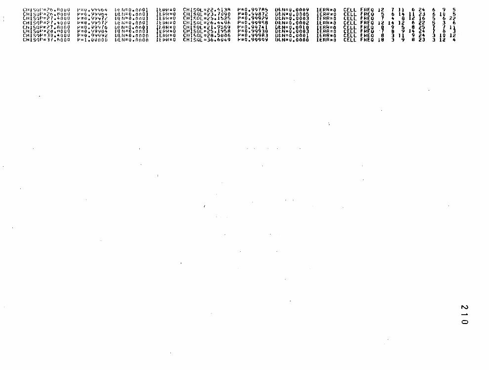
CtllS(Jf'=?t-.BOUO I' U • '14':ib4 t•tr~::o.oool IUm o CHISOL=22·'•1JR f'=0.997A!) l.li:.N=0.0009 lERA 0 CELL f"HF:Q 12 7 11 f> 21t 6 9 5 CHlSt)P=?.hol:lOOLl P o.~44b'l IJUl=O.ooOl lUll~ 0 CHISI~L"c3. 7090 P:o0.9CJ872 LJI:.N=o.ooos IERH 0 CELL fREQ 5 6 14 u 2J 6 10 5 C.HlS!lP=? 7.4000 P o.9'i"J7t: LJtN=o.oouJ lt.Rk 0 CHI~OL=c!:>.l!:>25 P=0.99929 lli:.N=O.OOOJ IERR 0 CELL f"HEQ 7 It 6 . 16 5 6 n CH1Sf1P=?7.400u I' tJ.9<J97C' liti•=O.OOOI li:.RI< 0 CHlSQL=t>&.449f> P=0.999'16 DI:.N=0.0002 IERH 0 CELL fREQ 12 14 12 6 22 5 3 6 u•prJP=?7 .Anoo I" 0.99476 IJ~.N=O.nool flRH 0 CHISOL=?.~·9559 P=0.99~41 ~I:.N"g.oo13 fiRR 0 E~~~ ~~~8 9 ~ ~ ,2 ~~ l ' 1 ~ t:fi $(JI-'=21:1oH000 ., o.<J99tl4 llEN=O.ooO trm o CH1SQL=2 .1958 P=O.'N 30 t.N= .ooo RA 0 CHJSQP::]0.4000 p 0.99492 IJtN=o.nooo llRH 0 Clll~QL=28.51:106 P=Oo999A3 lli:.N=O.OOOl II:.RR 0 CELL fREQ 6 3 Jl 9 24 3 10 12 CHJSQP=JI.f>OOO P I.ooooo IJLN=o.oooo lt PH 0 CHISOL=36o6049 P=0.9999'll OLN=o.oooo IERR 0 CELL fHEQ 18 3 9 8 23 3 12 4

N -0

APPEJ.'TDIX E

211

II t..: ~ ... ...

o .... c 0 coo Q ... _.N t"')

ooc 0 coo c: QOQ Q CCC 0 OCO C:

.. c: -II ~ ..... ¢

c

" :::;, ·~

o o c coc:u:::u~occ 0 Q c ocooccoc ._ IS' ..:; ,._CX:Cl'c:>-NI"l._ o e o oc::;:~~ ................. _. o c c cocoooc:e 0 0 0 COCO:tOQO c -= o co.ooecoo o o c cocceoeo

-1'1

c u

:::;, 0...• 1-0 ~~~ o:c nc. ..J>­

.JJ.JJ JlZ

-• -c:ru 'I..J -­z:r:- •. ,..

:r .I: :n II ll. :n -0

:n

z :;, 0 t.: u

" .[\ .,_ II J) :/1 II J) ~ 'J')·:;t- .... .D <Q. 0 11-.i--<l -1 Z 4' 0..'-'•Z-J u - "".J ·f)-~=--,.. .. u:c::c:::.-•-x<

=:3 zo=.::...; •'-'':l If .II "J4"'/)•>--__,,, _! -:\!!I~W>-~.._ JJ .'\: ..:;>JI:l,.-4-.Jiff) > a-~~'..J')...Jtt--a

...a n~~=-~~d---- _ --·-=z~~z--rz~ ~ ~~z~·-~J=~~~~n ~~ ~~=~>~0...~·~-~~> ~J~ CZ-~%·~~..J•C-~~z Ull~ ~-n•c=·~~..Jo--~-- ~~--~ ·~:-:~•·<~•·z=~ ==­-·~,r~~~z~~~-c~ -c~

- ~z~~-~r~O...Z~>UN~C~IIX ~ ~~-~~-~>~~%-~~WHU~~II ..J ~n~n~-n>nu•-r=~~~L..J

Z>f~lcn~~~~uc~~=c<~ = ~~~n~:-"n•>~~=~~zz~ --n~n~--zuu~~.~zn:~z

~~~~~~§;~~;~~~~~=~~ -~~--~- = .... ~--~- -

"".#It"~ ~ - - J --- .... ~.:l:.:l~lf ~ •=•=•=•«•~~~==~~=

~~~ ~ z ---- J-~-..J~~-------~ z~c~:J~~~J ~~;=~~~~~ ~=~~-,~,~, ~=~=~~~~n - ~ ~ ~~-~~-4"

;- ~~!~~~~ ~~;~~~~~tq ~~l ~------- --------~ C~J ~~~-~-~- -4~---~~ . ~-'<~=c=c::c::c=K~<~cx~~= "<c•-~-~-~-c-~<A~CACX

"" :"i...: -: .r.. 'f' _,. - f' .r ~

,.:_;:

" -:.. ."- -~

=- ..: = :: J.' :.rJ ·r './"'. J) <,{)

"- c "L.f

'' :- ..., . ' '" ..,

' ' ' ' r. f'; r. r. '' ;;; - .:l .J ... :.... -· ... .. ... " ~ - -

"' ~ ....................

,Il:::J':=J:>O"::l -.o-::-o-:;).:» ......;.'..-.. .... ..~... ......... "J...-'"V.r.-!':

~..a.J~::tOO-' -:;.t-t-~1-._1-

V'.-L.I.. ..... :.a.. .....

..... a. w :1!

0 ~ .... .... ... 1-11.1 loJ ..... ..1 ..1 0... .... LrJ IJJ 0 c ,.;

,. ~ ·~ "" :E 0 <1. - z 0 ~ 0 u a: VI

n :E I: ~ ..., -, .... "' c a- ~ :..; - _J

~ "' <: l: :::;

" 0 .::> 0 ~ 3

• .::;:1 .;:::, ·~ • -i..C!u..cf'­c:c::N::.:...-:c::c

)<; Q

J)

u ..J

" >J ~

\1

z <1. ~

u .... fJ \1 .., :

z ~

0 • "=> ·=- _-.J::.. :L. ~CC~=== =~...-:...-:...-:M>:- ~~VV~ifV ..., ______ -c:-~:-c•= ~:~~~~

..J < ,.... e ...

~

~

~· ·...; n '\J .J'I

0

z :<: ::

<t ~....J.tl....J .. "'l...J!:_i..,., i'"~_J J_J...) ..,;; ••. ...,.::-

~~---~- ,.; ~ ~ .n co~~K<~~-~~ -~~~~~~ .:: lf·_.l Jl f1!1 .;~II ;-,f'.J..:...U~ .... L . ...J~ .:-~'!1'1 4------ -~=·n~~~~-­zc~C4cc=~~~=-~n~··-~~o~M

..;...;....;t..;.;,.;._;o •Z •2.. •::: •2-'f:.J" f""': -·"': ~~~~~0~04 ~ ~ z ~~~ c..l~~..l..l..lc-~..,~~z-z~~ ~J~-'-'~-' n~~~~~n~~-cc~4c~~~JI-~-~~~--

..::.tr:. .- '../": - c-~~-~~--~-J ~C~>O~C~~~~ ~-~~-~- ~>~>~>~><C ....J.rt ~., n.n-e .r.::::: c::~_.-....,~•"z ,_..,:."'!-.r .:.--- :., ..... ...,

~ ~nn~z~

- .... ~---- . ..)-------~- ,,'\.. ..... -.~-"": \j•• ,, ..:-r------ .. 1~.r.r.-r.J.-J~:~: ...,., __ ~~~~~~n•~~=~=~~: -------Z~ \..i.\,;:'\.:"",.:"\,. .... ~ ~ ... ~ ... ·...: \,.:-..,. · .. "-... ·-------.._·;~. ~~-4~~~~~~~~~~~~ Z~~ZZ~<~« ~~~~~u-~~~-~~~~~ =~=~~~~~~ _._.,. ..... _____ .~ ...... ---~-

:: """ .... J ~~''''''':L ~ ,.. ,,

!'

:..l. ... _ ...... ... ... -- -_. _ _, _ _..._ __

--..: .:..:.= ."" :;_, -, .t ~, .... ' .......... ' ., ; . ...:::

,---:..,...~.:...l...:l.. :..~.:.."'"':....., .... ..~....!,. . .;....L. _..._ __ ._...._

_...._r------~.- .... --·J".v.v-.:..-::.r-.r .r--

'\J'"\...""\..'\..,"\.;.'\.."1 = = ::;~::::::J.·;. ......_._ ........ ~.....:.~ -------

2 1 2

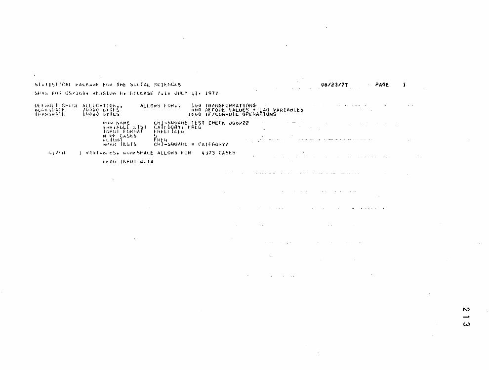
~J,,fJ<,TTC:III t'Al.~.,.,;r Ha~ Th!:. ~vill\l :"CH_t,ClS

SP<>:, fOil OS/Jt,(Jo 1/lHSl.!o'< ~., htli:A5t: l.i.t JIJLY 11• 1977

Ut. f 1\lil.l ')f-'ICC:t Wvl<r, '>f' AC~ I fi ll!•tSI' liC l

hI Vt 1·1

11LLL·C•• r 101''•. tur1uO "' Tf!:. llllluO t!Y ItS

ALL.O~·S t UHo • Juo fR~NSFOHMATlON.

kolr~ N"·f"t. VHh)/•Lill Ll!:.J I rwu I f CJt<~oA T N 1.'~ Lh~LS "t Horll .~,...,..'< n_sr~

4UO RFCOOL. VALUES + LAG V'HlAdL!:.S &bUO IF/CUMPUII: OPt:kATIONS

C.Hi-~OU~kt ltST CH!:.C~ JUd?2? C.Alt.GOHY t tRtC. IHrll Il:.tt• !J f Ht ~~ C:HJ-~IIUAI<t. :.: CAJf(;OkY/

V ,\,J( I,. t1i. t.!,, wur1t ';,I-' 1\Lf. IlL LOwS tOR

ld:AI1 Jl',f-UI IJ;,TA

4J73 CAStS

OIS/23177 PAGE

N __.

w

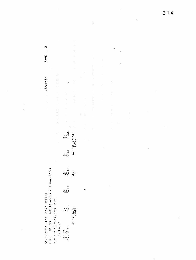
N

,_ ,_ ' . .., :\1

' 'X) 0

.\I '\;

" ..:: ~ , .: '..)

..... ;;;. ~

./1

.... cr c,

_,

;;;;. ..J

--' ..., ~

' ~ :

II

<t :::. z

<t ..., ..)

..J ~ o:".;:

-··

..; ~

_.,

" -J ~

-/1 I

:::. >-;,.,

-

"' <'..)

2 1 4

c 0 ....

u .!lCII> ...

<Ul u .... .-<:J' .... . .... ., -.

c ~ ~ .. . v;

~<t(fl

::> 0

...,cr.ro ~~

"' = . . . '\.10 .. ,

:;,

= --~""'.!' ::.:::. ~D

-:' . ..;;:,

.1'1 I

:...)

.=;

-....--.:z·...: --=..J... <..~:: ~

.:-- <

215

APPROVAl SHEET

The dissertation submitted by Adam J. Hiller II has been read and approved by the following committee:

Dr. Jack A. Kavanagh, :Jirector Associate Professor, Foundations, Loyola

:Dr. Samuel T. I.Tayo Professor, Foundations, Loyola

Dr. Steven I. Miller Associate Professor, Foundations, Loyola

The final copies have been examined by the director of the dis­sertation and the signature which appears below verifies the fact that &"ly necessary changes have been incorporated aDd that the dissertation is now given final approval by the Committee with reference to content and form.

The dissertation is therefore accepted in partial fulfillment of the requirements for the degree of uoctor of Education.

A orJ.'J3 J1'7?