A Monetary Business Cycle Model for India Shesadri Banerjee y Parantap Basu z Chetan Ghate x Pawan Gopalakrishnan { Sargam Gupta k September 11, 2017 Abstract This paper builds a New Keynesian monetary business cycle model with specic features of the Indian economy to understand why the aggregate demand channel of monetary transmission is weak. Our model allows us to identify the propagation mechanism and quantify the variance decomposition of a variety of real shocks (TFP, investment specic technological change, and scal policy) and nominal shocks (liq- uidity shocks, interest rate shocks) on the economy. In a specic environment, we show that scal dominance (in the form of a statutory liquidity ratio and adminis- tered interest rates) does not weaken monetary transmission. This is contrary to the consensus view in policy discussions in Indian monetary policy. We also show that a larger borrowing-lending spread, more aggressive ination and output targeting by the Central Bank weakens the transmission from the policy rate to output. Keywords : Monetary Business Cycles, Fiscal Dominance, Monetary Tranmission, Ination Targetting, Indian Macroeconomics JEL Codes :[JEL Codes here] We are grateful to PPRU (Policy Planning Research Unit) for nancial assitance related to this project. The views and opinions expressed in this article are those of the authors and no condential information accessed by Chetan Ghate during the monetary policy deliberations in the Monetary Policy Committee (MPC) meetings has been used in this article. y Madras Institute of Development Studies, Chennai 600020, India. Tel: 91-44-2441-2589. Fax: 91-44- 2491-0872. E-mail: [email protected]. z Durham University Business School, Durham University, Mill Hill Lane, DH1 3LB, Durham, UK. India. Tel: +44 191 334 6360. Fax: +44 191 334 6341. E-mail: [email protected]. x Corresponding Author: Economics and Planning Unit, Indian Statistical Institute, New Delhi 110016, India. Tel: 91-11-4149-3938. Fax: 91-11-4149-3981. E-mail: [email protected]. { Reserve Bank of India, Mumbai 400001, India. Tel: 91-22-2260-2206. E-mail: pawangopalakrish- [email protected]. k Economics and Planning Unit, Indian Statistical Institute, New Delhi 110016, India. Tel: 91-11-4149- 3942. Fax: 91-11-4149-3981. E-mail: [email protected]. 1

Welcome message from author
This document is posted to help you gain knowledge. Please leave a comment to let me know what you think about it! Share it to your friends and learn new things together.
Transcript
A Monetary Business Cycle Model for India�
Shesadri Banerjeey Parantap Basuz Chetan Ghatex
Pawan Gopalakrishnan{ Sargam Guptak
September 11, 2017
Abstract
This paper builds a New Keynesian monetary business cycle model with speci�c
features of the Indian economy to understand why the aggregate demand channel
of monetary transmission is weak. Our model allows us to identify the propagation
mechanism and quantify the variance decomposition of a variety of real shocks (TFP,
investment speci�c technological change, and �scal policy) and nominal shocks (liq-
uidity shocks, interest rate shocks) on the economy. In a speci�c environment, we
show that �scal dominance (in the form of a statutory liquidity ratio and adminis-
tered interest rates) does not weaken monetary transmission. This is contrary to the
consensus view in policy discussions in Indian monetary policy. We also show that a
larger borrowing-lending spread, more aggressive in�ation and output targeting by the
Central Bank weakens the transmission from the policy rate to output.
Keywords : Monetary Business Cycles, Fiscal Dominance, Monetary Tranmission,
In�ation Targetting, Indian Macroeconomics
JEL Codes :[JEL Codes here]
�We are grateful to PPRU (Policy Planning Research Unit) for �nancial assitance related to this project.The views and opinions expressed in this article are those of the authors and no con�dential informationaccessed by Chetan Ghate during the monetary policy deliberations in the Monetary Policy Committee(MPC) meetings has been used in this article.
yMadras Institute of Development Studies, Chennai �600020, India. Tel: 91-44-2441-2589. Fax: 91-44-2491-0872. E-mail: [email protected].
zDurham University Business School, Durham University, Mill Hill Lane, DH1 3LB, Durham, UK. India.Tel: +44 191 334 6360. Fax: +44 191 334 6341. E-mail: [email protected].
xCorresponding Author: Economics and Planning Unit, Indian Statistical Institute, New Delhi �110016,India. Tel: 91-11-4149-3938. Fax: 91-11-4149-3981. E-mail: [email protected].
{Reserve Bank of India, Mumbai � 400001, India. Tel: 91-22-2260-2206. E-mail: [email protected].
kEconomics and Planning Unit, Indian Statistical Institute, New Delhi �110016, India. Tel: 91-11-4149-3942. Fax: 91-11-4149-3981. E-mail: [email protected].
1
1 Introduction
With the formal adoption of in�ation targeting by the Reserve Bank of India, monetary
policy in India has undergone a major overhaul. With clearly de�ned objectives, operating
procedures, and a nominal anchor, the transmission mechanism of monetary policy has
become more transparent. India is now a �exible in�ation targeter, where a newly convened
monetary policy committee (as of September 2016) is tasked to maintain a medium term
CPI-headline in�ation at 4%, within a �oor of 2% and a ceiling of 6%.
Despite major changes in monetary policy however, monetary transmission has found to
be partial and asymmetric as well as slow (Das (2015); Mishra, Montiel and Sengupta (2016);
and Mohanty and Rishab (2016)). The lack of complete pass-through to bank lending and
deposit rates has also been a bugbear in recent monetary policy statements. These reports
routinely mention that the pass through of past policy rate cuts by the banking system should
be a pre-requisite for further rate cuts. Decomposing monetary transmission through the
bank lending channel in two steps - from policy rates to bank lending rates - and then from
lending rates to aggregate demand, Mishra, Montiel and Sengupta (2016) �nd that not only is
pass through from policy rate to banking lending rates incomplete, but there is little empirical
support for any e¤ect of monetary policy shocks on aggregate demand.1 Consistent with this,
the "Report of the Expert Committee to Strengthen the Monetary Policy Framework (2014)2,
also known as the Urjit Patel Committee Report, highlights several structural factors that
hinder monetary transmission in India, i.e., the role of �scal dominance in the form of SLR3,
small savings schemes (or administered interest rates), and the presence of a large informal
sector to name a few. The Urjit Patel Committee Report (2014) also notes that "... the
conduct of liquidity management (is) often mutually inconsistent and con�icting. Often,
increases in policy rate have been followed up with discretionary measures to ease liquidity
conditions (page 36)". Shocks to autonomous drivers of liquidity, such as currency demand,
bank reserves (required plus excess), government deposits with the Reserve Bank of India,
and net foreign market operations, complicate the alignment of the policy repo rate - the
short term signalling rate - with the overnight weighted average call rate (WACR) under the
liquidity adjustment facility.4
1Both Mishra, Montiel and Sengupta (2016) and Mohanty and Rishab (2016) provide excellent surveysof monetary transmission in India and emerging market developing economies (EMDEs) respectively.
2https://rbi.org.in/scripts/BS_PressReleaseDisplay.aspx?prid=304463The SLR, or the statutory liqudity ratio, provides a captive market for government securities and helps
to arti�cially suppress the cost of borrowing for the Government, dampening the transmission of interestrate changes across the term structure. See the Urjit Patel Commitee Report (2014).
4Since 2001, the Reserve Bank of India has conducted monetary policy through a corridor system calledthe LAF (liquidity adjustment facility). The LAF essentially allows banks to undertake collateralizedlending and borrowing to meet short term asset-liability mismatches. The Repo rate is the rate at which
2
This paper develops a New Keynesian monetary business cycle model of the Indian econ-
omy to understand why the aggregate demand channel of monetary transmission is weak.
As in Mishra, Montiel and Sengupta (2016), we de�ne the aggregate demand channel in two
steps: from policy rates to bank lending rates �and then from lending rates to GDP (includ-
ing its components, consumption and investment) and in�ation. We think that the aggregate
demand channel is important because consumption and investment constitute roughly 87%
of Indian GDP.
Our goal is two-fold. First, while there are a large number of empirical papers and policy
reports that study the strength of monetary transmission channels in the Indian context,
there are very few studies of monetary transmission in India using a DSGE model.5 Our
paper �lls this gap. Second, motivated by the role of �scal dominance in hindering monetary
transmission, our model embeds �scal dominance in monetary policy making in India by
incorporating two key features endemic to the Indian �nancial sector (i) SLR requirements
by banks, and (ii) administered interest rate setting by the government. Allowing for such
frictions in the banking sector helps us understand the role of banking intermediation in the
transmission of monetary impulses.
Our calibrated baseline model yields several results. First, we identify the propagation
mechanism of autonomous liquidity shocks, or autonomous base money shocks, to the rest
of the economy. We show that an expansionary base money shock stimulates consumption,
investment, hours worked, capital accumulation, and opens up a positive output gap on
impact. An increase in base money is also in�ationary. The rise in in�ation and the output
gap leads to a rise in the policy rate via the Taylor rule, which is equal to the short term
interest rate on government bonds. On the other hand, a fall in the government bond rate
also has similar expansionary e¤ects on the economy.
Second, our baseline model shows that about half of the �uctuation (variance) in output
are explained by TFP shocks and one third is explained by �scal shocks. Monetary policy in
terms of interest rate shocks and base money shocks explain a negligible fraction of output
variation exemplifying the weak transmission channel of monetary policy.
Third, our sensitivity experiments with respect to structural and policy parameters indi-
cate that household�s preference for commercial bank deposits vs postal deposits (or deposits
with administered interest rates), the statutory liquidity ratio, and administered interest
rates have negligible e¤ects on the monetary transmission channel measured by the forecast
banks borrow money from the RBI by selling short term government securities to the RBI, and then "re-purchasing" them back. A reverse repo operation takes place when the RBI borrows money from banks bylending securities. See Mishra, Montiel and Sengupta (2016, pages 73-74).
5See Levine et al. (2012) for an early attempt. Banerjee and Basu (2017) develop a small open DSGEmodel for India but do not study the monetary transmission mechanism.
3
error variance of output due to autonomous monetary shocks or the money-output correla-
tion. While this result is speci�c to the way we have modelled the banking sector�s problem,
this observation itself can be treated in the context of policy discussion on monetary trans-
mission. In this speci�c environment, neither administered interest rate nor �scal dominance
(in the form of SLR) cause weak monetary transmission in the economy as it is widely be-
lieved. On the other hand, a larger borrowing-lending spread and less aggressive in�ation
and output targeting makes the monetary policy transmission resulting from a policy rate
shock weaker and the e¤ect of autonomous shocks to monetary base stronger.
Fourth, our sensitivity analysis suggests that a higher long term interest rate on gov-
ernment bond weakens monetary transmission and raises the importance of �scal spending
shocks. This happens because a higher long term policy rate necessitates higher taxes to
retire outstanding public debt. This highlights �scal dominance in our model.
The paper is organized as follows. In the next section, we lay out our model. Section 3
is devoted to a quantitative analysis of the model. Section 4 concludes.
2 The Model
2.1 Environment
Our core model is a monetary RBC model with sticky prices. On the household and produc-
tion side, the model economy is similar to Gerali et al. (2010) but with important di¤erences.
The economy is populated by households and entrepreneurs, each group having unit mass.
Households consume, work, and accumulate savings in risk-free bank deposits as well as
postal deposits with a �xed government set interest rate.6 We assume that households own
the banks. On the production side, wholesale entrepreneurs produce homogenous interme-
diate goods using capital, bought from capital goods producers, loans obtained from banks,
and hired labor from households. As in Gerali et al (2010), capital goods producers are
introduced to derive a market price for capital. A monopolistically competitive retail sector
buys intermediate goods from wholesale entrepreneurs, and produces a single �nal good.
Retail prices are sticky and indexed to steady state in�ation: This allows monetary policy
to have real e¤ects. Retailers also face a quadratic price adjustment cost a la Rotemberg.
Unlike Gerali et al (2010), banks in the current set-up are assumed to be perfectly
competitive.7 Banks maximize cash �ows in every period, o¤er savings deposits to households
and loans to wholesale entrepreneurs, subject to the constraints that a �xed fraction of
6In Gerali et al. (2010), there are no administered postal accounts.7Market power in the banking industry in Gerali et al. (2010) is modelled using a Dixit-Stiglitz framework
for retail and credit deposit markets.
4
deposits in every period are set aside for (i) a statutory liquidity requirement (SLR) and (ii)
reserve requirements. We allow for the stochastic withdrawal of deposits in each period as
in Chang et al. (2014). At date t; if the withdrawal, exceeds bank reserve (cash in vault),
banks fall back on the Central Bank for emergency loans at a penalty rate mandated by the
central bank: The presence of SLR requirements and administered interest rates capture the
essence of �scal dominance in the Indian economy.
We assume that the central bank is a �exible in�ation targeter, as in India. There is
no currency in the model, and so the supply of reserves equals the monetary base. The
central bank lets the monetary base, or the supply of reserves increase by a simple rule
that is perturbed in every period by base-money shocks, or autonomous liquidity shocks. In
addition to these shocks, the economy is also hit in every period by total factor productivity
shocks, �scal policy shocks, investment speci�c technology (IST) shocks, and interest rate
shocks. To deal with the in�ationary consequences of autonomous liquidity shocks, the
central bank has one instrument at its disposal: the short term interest rate on government
bonds, which we interpret as the policy rate, and which is governed by a conventional Taylor
rule. The economy is hit periodically with autonomous liquidity, or base money shocks,
which are in�ationary, and therefore warrant a monetary policy response using the Taylor
rule.
On the �scal side, the government spends stochastically and issues public debt held by
banks to cover the di¤erence between government spending and lump sum taxes. Adminis-
tered postal deposits, which attract a government set interest rate in the Indian economy,
are directly assumed to augment government revenues in every period.
We calibrate the model and provide a baseline parameterization that can replicate the
regularities of the Indian business cycles broadly. Then, we focus on impulse response prop-
erties and variance decomposition results to highlight and explain the role of shocks and
frictions on monetary transmission.
2.2 Households optimization
The economy is populated by in�nitely lived households of unit mass. The representative
household maximizes expected utility
maxCt;Ht;Dt+1;D
pt+1
E0
1Xt=0
�t[U(Ct)� �(Ht) + V (Dt=Pt; Dat =Pt)] (1)
which depends on hours worked, Ht; consumption of the �nal good, Ct; and saving in the
form of risk-free bank and postal deposits, Dt; and Dat respectively. Household choices must
5
obey the following budget constraint (in nominal terms)
Pt (Ct + Tt) +Dt +Dat � WtHt + (1 + i
Dt )Dt�1 + (1 + i
a)Dat�1 +�
kt +�
rt (2)
The left hand side of equation (2) represents the �ow of expenses which includes current
consumption (where Pt is the aggregate price index and Tt > 0 denote lump-sum transfers),
nominal bank deposits, Dt and postal deposits, Dat : Resources consist of wage earnings,
WtHt; where Wt is the wage rate, payments on deposits made in the previous period, t� 1;where iDt > 0 is the rate on one-period deposits (or savings contracts) in the banking system,
and ia > 0 is the �xed government administered interest rate on postal deposits made by
households. �kt and �rt denote nominal pro�ts rebated back from the capital goods sector,
and the retail goods sector, to households respectively.8
Using Dt=Pt = dt and Dat =Pt = dat , and substituting out for U
0(Ct) = �tPt; we can
re-write the household�s optimality conditions as:
Dt : U0(Ct) = V
01(dt; d
at ) + �U
0(Ct+1)(1 + iDt+1)(Pt=Pt+1); (3)
Dpt : U
0(Ct) = V02(dt; d
at ) + �U
0(Ct+1)(1 + ia)(Pt=Pt+1) (4)
�0(Ht) = (Wt=Pt)U0(Ct): (5)
Equation (3) is the standard Euler equation for deposits. Equation (4) is the Euler
equation for postal deposits which attract the administered interest rate, ia:Equation (5) is
the standard intra-temporal optimality equation for labor supply.
2.3 Capital good producing �rms
Our description of the capital goods producing �rms is standard. Perfectly competitive
�rms buy last period�s undepreciated capital, (1 � �k)Kt�1; at price Qt from wholesale-
entrepreneurs (who own the �rms) and It units of the �nal good from retailers at price Pt:
The transformation of the �nal good into new capital is subject to adjustment costs; St:9
Capital goods producing �rms maximize
8Please refer to Appendix A for all derivations.9 We assume that
S
�ItIt�1
�= (�=2)
�ItIt�1
� 1�2:
6
maxItEt
1Xj=0
t;t+jPt+j
�Qt+jIt+j �
�1 + S
�It+jIt+j�1
��It+j
�(6)
s.t. Kt = (1� �k)Kt�1 + Zx;tIt (7)
where t;t+j is the stochastic discount factor and Zx;t is an investment speci�c technology
(IST) shock that follows an AR(1) process.
The �rst order condition is
@ (:)
@It= t;tPtQt�t;tPt
�1 + S
�ItIt�1
���t;tPtS 0
�ItIt�1
�ItIt�1
+t;t+1Pt+1S0�It+1It
��It+1It
�2= 0:
(8)
which yields the capital good pricing equation,
Qt = 1 + S
�ItIt�1
�+ S 0
�ItIt�1
�ItIt�1
� �EtU 0 (Ct+1)
U 0 (Ct)
"S 0�It+1It
��It+1It
�2#: (9)
2.4 Wholesale good producing �rms
Wholesale, or intermediate goods �rms are run by risk neutral entrepreneurs who produce
intermediate goods for the �nal good producing retailers in a perfectly competitive envi-
ronment. The entrepreneurs hire labor from households and purchase new capital from the
capital good producing �rms. They borrow an amount Lt > 0 of loans from the bank in
order to meet the value of new capital, QtKt; where Kt is the capital stock. We assume that
all capital spending is debt �nanced. Used capital at date t+ 1 is sold at the resale market
at the price Qt+1: The balance sheet condition of the wholesale �rms is:
QtKt =
�LtPt
�: (10)
In the steady state Qt = 1 which means lt = LtPt= Kt; i.e., all capital is intermediated. The
production function for a representative wholesale goods producer is given by
Y Wt = �atK�t�1H
1��t
with 0 < � < 1: �at denotes stochastic total factor productivity, and follows an AR(1)
process. The (real) wage rate, Wt; is given by
7
Wt=Pt = (PWt =Pt)MPHt = (1� �)
(PWt =Pt)YWt
Ht(11)
This allows us to obtain the rate of rate of return from capital,1 + rkt+1; as
1 + rkt+1 =(PWt+1=Pt+1)Y
Wt+1 � (Wt+1=Pt+1)Ht+1 + (1� �k)KtQt+1
QtKt
=(PWt+1=Pt+1)
�YWt+1Kt
�� (1� �) (P
Wt+1=Pt+1)Y
Wt+1
Ht+1
�Ht+1Kt
�+ (1� �k)Qt+1
Qt
=(PWt+1=Pt+1)MPKt+1 + (1� �k)Qt+1
Qt
The optimality condition for a �rms�demand for capital is given by the following arbitrage
condition,
1 + rkt+1 =�1 + iLt+1
� PtPt+1
: (12)
This yields,
(1 + iLt+1) =PWt+1MPKt+1 + (1� �k)Pt+1Qt+1
PtQt
1 + iLt+1 =
��Pwt+1Pt+1
�MPKt+1
Qt+1+ 1� �k
� �Pt+1Qt+1PtQt
�: (13)
2.5 Final good retail �rms
Retailers buy intermediate goods at price PWt and package them into �nal goods and operate
in a monopolistically competitive environment as in Bernanke, Gertler, and Gilchrist (1999).
They convert the ith variety of the intermediate good, yWt (i) ; into yt (i) one-to-one and
di¤erentiate the goods at zero cost. Each retailer sells his unique variety of �nal product
after applying a markup over the wholesale price, and factoring in the market demand
condition which is characterized by price elasticities�"Y�: Retailer�s prices are sticky and
indexed to past and steady state in�ation as in Gerali et al. (2010): If retailers want to
change their price over and above what indexation allows, they have to bear a quadratic
adjustment cost given by �p:
Retailers choose fPt+j (i)g1j=0 to the maximize present value of their expected pro�t.
maxPt(i)
Et
1Xj=0
t;t+j��rt+jjt
(14)
subject to the demand constraint, yt+jjt (i) =�Pt+j(i)
Pt+j
��"Yyt+j; where the pro�t function of
8
the ith retailer is given by,
�rt (i) = Pt (i) yt (i)� PWt (i) yWt (i)��p2
"�Pt+j (i)
Pt+j�1 (i)� (1 + �t�1)�p(1 +
��)1��p
�2Ptyt
#(15)
�p > 0, 0 < �p < 1; and
yt =
�Z 1
0
yt (i)"Y �1"Y di
� "Y
"Y �1
; "Y > 1:
Note that �p is an indexation parameter. This price adjustment cost speci�cation is borrowed
from Gerali et al (2010). The �rst order condition after imposing a symmetric equilibrium
is standard:
1� "Y + "Y ( PtPWt
)�1 � �pn1 + �t � (1 + �t�1)�p(1 +
��)1��p
o: (16)
In the steady state, when �t+1 = �t = �; this implies that the steady state mark-up is,
P
PW=
"Y
"Y � 1 : (17)
2.6 Banks
The representative bank maximizes cash �ows by o¤ering savings contracts (deposits) and
borrowing contracts (loans) Banks are also mandated to keep reserves with the central bank.
In India, and many other emerging market economies (EMEs), they are also constrained to
buy government debt from deposit in�ows as mandated by a statutory liquidity ratio (SLR)
In every period, following Chang et al. (2014), we assume that banks face a stochastic
withdrawal of deposits at the end of each period, t. At date t; if the withdrawal (say ]Wt�1)
exceeds bank reserve (cash in vault), banks fall back on the Central Bank for emergency loans
at a penalty rate ip mandated by the Central Bank (CB): Banks pay back the emergency
borrowing to the CB at the end of the period. This withdrawal uncertainty necessitates a
demand for excess reserve by the banks.10
10A practical application of the stochastic withdrawl is as follows. Suppose the withdrawal of deposits isexpected at the end of the period. Suppose the bank anticipates that it will fall short of reserve by x rupeesat the end of the day. charges a y percent penalty rate. Thus the bank�s expected penalty is x(1+ y) rupeeswhich includes the principal and interest that the bank has to pay at the end of the period or the start ofthe next period. Taking this into consideration, the bank chooses its reserve holding optimally at the startof date t. Thus a higher expected penalty will make the bank hold more cash reserve.
9
De�ne iLt to be the interest rate on loans, Lt�1, iR to be the interest rate on reserves,MR
t ;
mandated by the central bank, and fWt is the stochastic withdrawal. Since government bond
and short term deposits are perfect substitutes, iDt = iGt = i
st (say). Dt denotes deposits. We
assume that bank has a SLR equal to �s 2 [0; 1]:The bank�s cash �ow at date t can be rewritten as:
CF bt = (1 + iLt )Lt�1 + (1 + i
R)MRt�1 + �s(1 + i
Gt )Dt�1| {z }
SLR on last period�s deposits
� (1 + iDt )Dt�1| {z }Cost of Funds of Last period�s Deposits
(18)
� (1 + ip)Emax(]Wt�1 �MRt�1; 0) + Dt|{z}
Current Deposits
� �sDt| {z }SLR this period
� Lt �MRt
The �rst two terms on the right hand side correspond to the interest earned in time t on
loans disbursed in time t � 1, and interest on reserves in the previous period, MRt�1: Since
the bank is forced to hold government debt as a constant fraction, �s; of incoming deposits,
�s(1+ iGt )Dt�1, denotes the interest earnings on SLR debt holdings by banks As described
above, banks also face a penalty, at a constant penal rate, ip > 0; for stochastic withdrawals
over and above their bank reserves. The penalty amount is (1 + ip)Emax(]Wt�1 �MRt�1; 0).
We assume that banks o¤er a deposit rate, iDt ; which is a mark-down of the interest rate that
it receives on government bonds, iGt . In other words, 1 + iDt = �(1 + i
Gt ) where 0 < � < 1.
We do not model the mark-down, �, but calibrate it. Rewrite the cash �ow in equation (18)
as
CF bt = (1 + iLt )Lt�1 + (1 + i
R)MRt�1 � (� � �s)(1 + iGt )Dt�1 (19)
� (1 + ip)Emax(]Wt�1 �MRt�1; 0)
+ (1� �s)Dt � Lt �MRt :
The representative bank maximizes discounted cash �ows in two stages. It �rst solves for its
optimal demand for reserves, MRt : Next, it chooses the loan amount, Lt. Speci�cally, banks
maximize
MaxMRt ;;Lt
Et
1Xs=0
t;t+sCFbt+s
10
subject to the statutory reserve requirement:
MRt = �rDt (20)
where t;t+s =�sU 0(ct+s)U 0(ct)
: PtPt+s
is the in�ation adjusted stochastic discount factor.
The Euler equation is given by11
Ett;t+1
"(1 + iR) + (1 + ip)
Z Dt
MRt
f(fWt)dfWt
#+ �t = 1 (21)
The �rst term in the square bracket in equation (21) is the bank�s interest income from
reserves. The second term is the expected saving of penalty because of holding more reserves
�t is the Lagrange multiplier associated with the reserve constraint (20). The Kuhn Tucker
condition states thatMRt
Dt
= �r if �t > 0
Assume that the reserve requirement is not binding, which implies that �t = 0:Assuming a
rectangular distribution for fWt over [0; Dt]12, (21) reduces to:
MRt : 1 = Ett;t+1
�(1 + iR) + (1 + ip)(1� M
Rt
Dt
)
�: (22)
We solve MRt
Dtas follows:
MRt
Dt
= 1� 1� (1 + iR)Ett;t+1
(1 + ip)Ett;t+1(23)
which is the same as writing
xtdt= 1� 1� (1 + i
R)Ett;t+1(1 + ip)Ett;t+1
(24)
where xt = MRt =Pt and dt = Dt=Pt. It is straightforward to verify that given the discount
factor, t;t+1; a higher iR or ip means a higher MRt as expected.
Once the bank�s reserve demand problem is solved, we next turn to the holding of loans.
Note that the bank solves a recursive problem of choosing Lt given Lt�1 which were chosen
in the previous period. This is a dynamic allocation problem. The �rst order condition with
11See Technical Appendix A.12 Since fWt follows a rectangular distribution, over [0; Dt]Z Dt
MRt
f(fWt)dfWt =Dt �MR
t
Dt= 1� M
Rt
Dt:
11

respect to Lt is given by,
t;t(�1) + Ett;t+1(1 + iLt+1) = 0:
This gives the loan Euler equation:
Lt : 1 = Ett;t+1(1 + iLt+1) (25)
Substituting out for Ett;t+1 in equation (25) and putting it into equation (23), we see the
following connection between the loan market premium and the reserve demand of bank:
xtdt= 1 +
1 + iR
1 + ip
241� Et1+iLt+11+iR
1� covt(t;t+1; (iLt+1 � iR))
35 (26)
The negative of the covariance term in the denominator picks up the risk premium associated
with the risky loan of banks relative to the risk-free interest rate on reserves. If the bank
loan is not risky, this covariance term is zero in which case a higher loan rate discourages the
holding of bank reserves. However, if the loan is a bad hedge which makes the absolute value
of the covariance bigger, it will encourage banks to hold more reserves which is reminiscent
of the �nancial crisis.13
2.7 Monetary Policy
The Central Bank follows a simple money supply rule. It lets the monetary base (MBt ), or
the supply of reserves, MRt (since currency is zero), increase by the following rule:
MBt =M
Bt�1
1 +��
=
MBt�1=M
Bt�2
1 +��
!��exp(��t ) (27)
13One may wonder whether there is any borrowing-lending spread because banks are not monopolistic.Curiously a steady state borrowing-lending spread still emerges in this model because deposit appears in theutility function and provides a liquidity service (convenience yield) to the household. Bank deposit providessome transaction utility to the household. Thus the household wishes that the banks do not loan out alltheir deposits and make them illiquid. This convenience yields (alternatively a liquidity premium) gives riseto a credit rationing which gives rise to a positive borrowing-lending spread in the steady state. To see itcombine (3) and (25) to get the following steady state borrowing-lending spread.
iL � iD = (1 + �)
�
V0
1 (d; dp)
U 0(c)> 0
This conveience yield is akin to forward-spot spread in �nance.
12
where �� is the policy smoothing coe¢ cient and ��t is the money supply shock, which follows
an AR (1) process. We view a shock to the monetary base as an autonomous liquidity shock.
Money market equilibrium implies that
MRt =M
Bt for all t:
Such a money supply process imposes restriction on the short run growth rate of real reserve
and in�ation as follows:
(1 + �t)(xt=xt�1)
1 + �=
�(1 + �t�1)(xt�1=xt�2)
1 + �
���exp(��t ) (28)
Since real reserves are proportional to deposits as shown in the bank�s reserve demand
function, this also imposes imposes restriction on the dynamics of deposits, interest rate on
loans and consumption.
2.8 Interest rate policy
The short term interest rate on government bonds (iGt ) can be broadly interpreted as a policy
rate. We give it an in�ation targeting Taylor rule as follows:
(1 + iGt )
(1 +�iG)
=
0@(1 + iGt�1)(1 +
�iG)
1A�iG ��
1 + �t�11 + �
�'� �YtY
�'y�(1��iG)exp(�Gt ) (29)
The parameters �p > 0 , and �y > 0 are the in�ation, and output gap sensitivity parameters
in the Taylor Rule. Yt denotes GDP, and therefore YtYdenotes the output gap. �iG is the
interest rate smoothing term and �Gt is the policy rate shock.
We shall see later in the quantitative analysis section that the strength of monetary
transmission of a money base shock is signi�cantly in�uenced by the parameters of the
Taylor rule.
2.9 Fiscal Policy
The government budget constraint (in nominal terms) is given by,
PtGt+�1 + iGt
�Bt�1+(1+i
R)MRt�1+(1+i
a)Dat�1 = PtTt+Bt+M
Rt +D
at+(1+i
p)Emax(fWt�MRt ; 0)
(30)
where Gt corresponds to real government purchases, Bt and denotes the stock of public debt.
The left hand side of equation (30) denotes total expenditures by the government (nominal
13
government purchases + interest payments on public debt + interest rates on reserves +
interest payments on administered postal deposits).14 The right hand side of equation (30)
denotes the total resources available to the government (nominal lump sum taxes + new debt
+ new reserves + administered deposits + interest payments from withdrawal penalties).
Government spending (or government purchases) evolves stochastically according to:
Gt ��G = �G
�Gt�1 �
�G
�+ �Gt :
�Gt denotes the shock to government spending, and follows an AR(1) process.
2.10 Steady State
In this section, we solve for the steady state values of the endogenous variables. Equation
(13) in the steady state is given by,
1 + iL =
��PW
P
�MPK
Q+ 1� �K
�(1 + �)
as Pt+1Pt
= 1 + �t. Further, from equation (9) and (17) in the steady state, Q = 1 and
PW = "Y �1"YP , respectively. Also, in the steady state, Y W = K�H1�� which implies that
MPK = �YW
K. The above equation thus reduces to,
1 + iL =
��"Y � 1"Y
���Y W
K
�+ 1� �K
�(1 + �) (31)
Recalling that in the steady state, the stochastic discount factor is given by �1+�; substituting
this into the steady version of equation (25) yields, 1+ iL = (1+�)�. From this expression, we
can solve for the steady state capital-labor ratio, K=H, which is given by
K
H=
(�
�"Y � 1"Y
�"1
1�� (1� �K)
#) 11��
(32)
which we call � hereafter.
The national income identity is given by,
C + �KK +G = K�H1�� (33)
14We think of the government as a combined �scal-monetary entity.
14
Assume the following functional forms: � (Ht) = Ht, U (Ct) = ln (Ct) and V (dt; dat ) =
� ln dt + (1� �) ln dat . Thus in steady state, �0 (H) = 1, U 0 (C) = 1=C; V 01 (:; :) =�dand
V 02 (:; :) =(1��)da: Substituting for these values into equation (5) ; in the steady state, we get
C = W=P
Next note from (11) and (17), W=P = (1� �)�"Y �1"Y
� �KH
��: Therefore,
C = (1� �)�"Y � 1"Y
�(�)� : (34)
Now, substituting V 01 (:; :) =�din equation (3), we get,
1
C= V
0
1 (:; :) + �1
C
�1 + iD
�(1 + �)
The above can be re-written as,
1 + iD=1 + � � �C
d(1 + �)
�(35)
Similarly substituting V 02 (:; :) =(1��)da: in equation (4) ;we get,
1 + ia =1 + � � (1� �) C
da(1 + �)
�(36)
Since KH= �; equation (33) above thus reduces to,
C +G =���(1��) � �K
�K (37)
Recall, from equation (30) the government budget constraint is given by,
PtGt+�1 + iG
�Bt�1+(1+i
R)MRt�1+(1+i
a)Dat�1 = PtTt+Bt+M
Rt +D
at+(1+i
p)Emax(fWt�MRt ; 0)
Dividing throughout by Pt and noting thatPt+1Pt= 1 + �t; we get
Gt+�1 + iGt
� bt�11 + �t
+(1+iRt )xt�11 + �t
+(1+ia)dat�11 + �t
= Tt+bt+xt+dat+(1+i
pt )dtEmax(
fWt
Dt
�MRt
Dt
; 0)
where xt =MRt =Pt, dt =
DtPt; and bt = Bt=Pt:
In the steady state, the above equation becomes
15
Gt+�1 + iGt
� b
1 + �+(1+iRt )
x
1 + �+(1+ia)
da
1 + �= T+b+x+da+(1+ipt )dEmax(
fWt
Dt
�MRt
Dt
; 0);
or,
G(1 + �) +�iG � �
�b+ (iR � �)x+ (ia � �)da = T + (1 + ip)dEmax(
fWt
Dt
� MRt
Dt
; 0)
Dividing through the above expression by d; yields,
G(1 + �)
d+�iG � �
��s + (i
R � �)xd+ (ia � �)d
a
d= T + (1 + ip)Emax(
fWt
Dt
� MRt
Dt
; 0) (38)
since B=D = �s (which implies b=d = �s) Also,xd =MR=PD=P
:
We can substitute out for da
din the above equation (38) from equation (35) and (36)
nothing that.
d�1 + � � �
�1 + iD
��= �C(1 + �)
da [1 + � � � (1 + ia)] = (1� �)C(1 + �)
or,d
da=
�
1� �
�1 + � � � (1 + ia)1 + � � � (1 + iD)
�; (39)
andx
d= 1�
1� (1 + iR) �1+�
(1 + ip) �1+�
:
Finally, let us solve for Emax(fWt
Dt� MR
t
Dt; 0) in the steady state: Assume fWt
Dt= Zt; and since
Dt is given, Zt follows an uniform distribution as fWt but between [0; 1]: Thus,
Emax(Zt �MRt
Dt
; 0) =
Z 1
MRt =Dt
�Zt �
MRt
Dt
�h (Zt) dZt
16
Since h (Zt) = 1;
Emax(Zt �MRt
Dt
; 0) =
Z 1
MRt =Dt
�Zt �
MRt
Dt
�dZt
=Z2t2
����1MRt =Dt
� MRt
Dt
Ztj1MRt =Dt
=
0B@1��MRt
Dt
�22
1CA� MRt
Dt
�1� M
Rt
Dt
�
=1
2+1
2
�MRt
Dt
�2� M
Rt
Dt
= 0:5
�1� M
R
D
�2(40)
where MR
Dis given by (23) evaluated at the steady state.
Continuing from the above government constraint (38) we get
G(1 + �)
d+�iG � �
��s+(i
R��)xd+(ia��)d
a
d= T+(1+ip)0:5
1�
(1�
1� (1 + iR) �1+�
(1 + ip) �1+�
)!2(41)
From the above equation, we can solve for steady state lump-sum taxes, T: In Technical
Appendix B, we summarize the steady state equations in recursive form.
3 Quantitative Analysis
The objective of our quantitative analyses is to understand the monetary transmission mech-
anism for the baseline model. Monetary transmission implies how a monetary policy impacts
the aggregate economy. As mentioned in the introduction, we de�ne that the aggregate de-
mand channel operates in the model economy via two layers: from policy rates to bank
lending rates, and then, from lending rates to GDP (including its components of consump-
tion and investment) and in�ation. For this purpose, we focus on the standard instruments
of monetary policy for an in�ation targeting central bank (i) money base and (ii) short term
interest rate (which is the government bond rate in our model). We examine the magnitude
of transmission of the shocks from policy instruments to policy targets, primarily, using the
results of a variance decomposition of key macroeconomic variables of the model economy.
Parallel to this, we also consider the magnitude of cross correlations between the policy in-
struments and policy targets as the indicators of pass through of the policy shocks. To this
17
end, �rst, we specify the parameterization of the baseline model and then, validate the same
with data by moment matching exercise.
We calibrate the model based on Indian macroeconomic data and evidence from the
DSGE literature based on the Indian economy. After baseline con�guration and validation
with data, we explain the impulse response properties of the model followed by the variance
decomposition results. Next, we present the variance decomposition results of counterfactual
experiments which document the role of di¤erent structural and policy factors in determining
the strength of monetary transmission. Finally, we present the results of our experiments on
di¤erent degrees of �scal dominance driven by di¤erent steady state policy rates which have
some implications for weakening the monetary transmission channel.
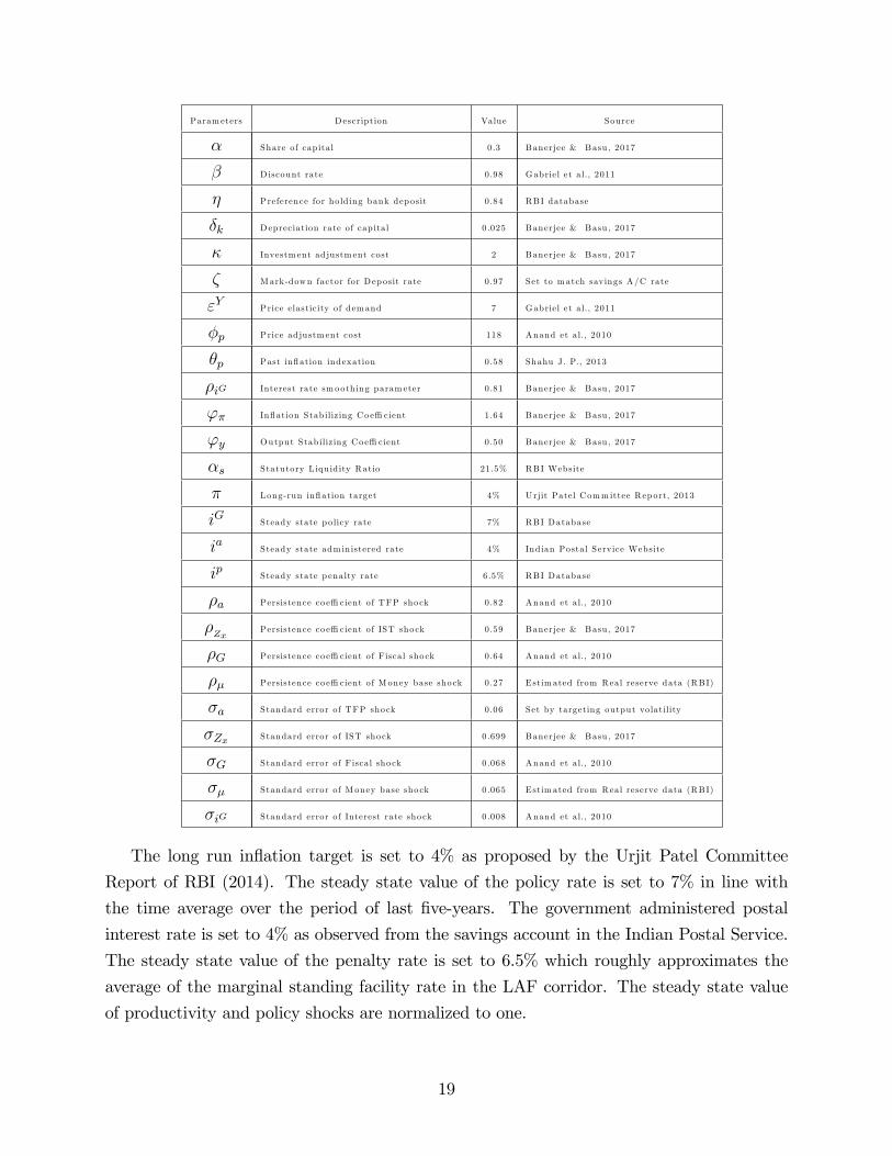
3.1 Baseline Parameterization
Following the DSGE literature on India and using Indian data on the macroeconomic vari-
ables, we calibrate the parameters of our model. Baseline parameterization of the model
is presented in Table 1. The share of capital in production process is set as 0.3 (Banerjee
and Basu, 2017). The discount factor is taken as 0.98 (Gabriel et al., 2012). Household�s
preference for holding bank deposits is calibrated based on the share of commercial bank
deposits to total deposits which is approximately 84%. Depreciation of physical capital is
chosen as 2.5% on a quarterly basis. Investment adjustment cost parameter is set to 2 from
Banerjee and Basu (2017). The mark down factor for the deposit interest rate is taken as
0.97 in order to match the savings account deposit rate at the steady state of 3.8%. Price
adjustment cost parameter is taken as 118 from Anand et al. (2010) and indexation of past
in�ation is set to 58% following Sahu (2013). Policy parameters for the Taylor rule stabilizer
are chosen from Banerjee and Basu (2017), where interest rate smoothing coe¢ cient is 0.81,
in�ation stabilizing coe¢ cient is 1.64, and output gap stabilizing coe¢ cient is 0.50. In India,
the statutory liquidity requirement of the commercial banks is 21.5%, and the value of �s is
set accordingly.
Table 1: Baseline Parameterization
18
Param eters Description Value Source
� Share of cap ita l 0 .3 Banerjee & Basu , 2017
� Discount rate 0.98 Gabriel et a l., 2011
� Preference for hold ing bank deposit 0 .84 RBI database
�k Depreciation rate of cap ita l 0 .025 Banerjee & Basu , 2017
� Investm ent adjustm ent cost 2 Banerjee & Basu , 2017
� Mark-down factor for Deposit rate 0.97 Set to match savings A/C rate
"Y Price elastic ity of demand 7 Gabriel et a l., 2011
�p Price adjustm ent cost 118 Anand et al., 2010
�p Past in�ation indexation 0.58 Shahu J. P., 2013
�iG Interest rate smooth ing param eter 0.81 Banerjee & Basu , 2017
'� In�ation Stab iliz ing Coe¢ cient 1.64 Banerjee & Basu , 2017
'y Output Stab iliz ing Coe¢ cient 0.50 Banerjee & Basu , 2017
�s Statutory L iqu id ity Ratio 21.5% RBI Website
� Long-run in�ation target 4% Urjit Patel Comm ittee Report, 2013
iG Steady state p olicy rate 7% RBI Database
ia Steady state adm in istered rate 4% Indian Postal Serv ice Website
ip Steady state p enalty rate 6.5% RBI Database
�a Persistence co e¢ cient of TFP shock 0.82 Anand et al., 2010
�Zx
Persistence co e¢ cient of IST shock 0.59 Banerjee & Basu , 2017
�G Persistence co e¢ cient of F isca l sho ck 0.64 Anand et al., 2010
�� Persistence co e¢ cient of M oney base sho ck 0.27 Estim ated from Real reserve data (RBI)
�a Standard error of TFP shock 0.06 Set by targeting output volatility
�Zx Standard error of IST sho ck 0.699 Banerjee & Basu , 2017
�G Standard error of F isca l sho ck 0.068 Anand et al., 2010
�� Standard error of M oney base sho ck 0.065 Estim ated from Real reserve data (RBI)
�iG Standard error of Interest rate sho ck 0.008 Anand et al., 2010
The long run in�ation target is set to 4% as proposed by the Urjit Patel Committee
Report of RBI (2014). The steady state value of the policy rate is set to 7% in line with
the time average over the period of last �ve-years. The government administered postal
interest rate is set to 4% as observed from the savings account in the Indian Postal Service.
The steady state value of the penalty rate is set to 6.5% which roughly approximates the
average of the marginal standing facility rate in the LAF corridor. The steady state value
of productivity and policy shocks are normalized to one.
19
First order persistence and standard error of the TFP (0.82 and 0.06 respectively) and
�scal policy (0.64 and 0.068 respectively) shocks are in line with Anand et al. (2010). For
the IST shock, the estimates for AR (1) coe¢ cient and standard error are 0.59 and 0.699
respectively (Banerjee and Basu, 2017). In case of the autonomous shock to money base,
we simply estimate an AR (1) process with the data on growth rate of real reserve. The
persistence coe¢ cient is found to be 0.27 while the standard error takes value of 0.065.
Finally, the standard error of the policy rate shock is set to 0.008 following Anand et al.
(2010).
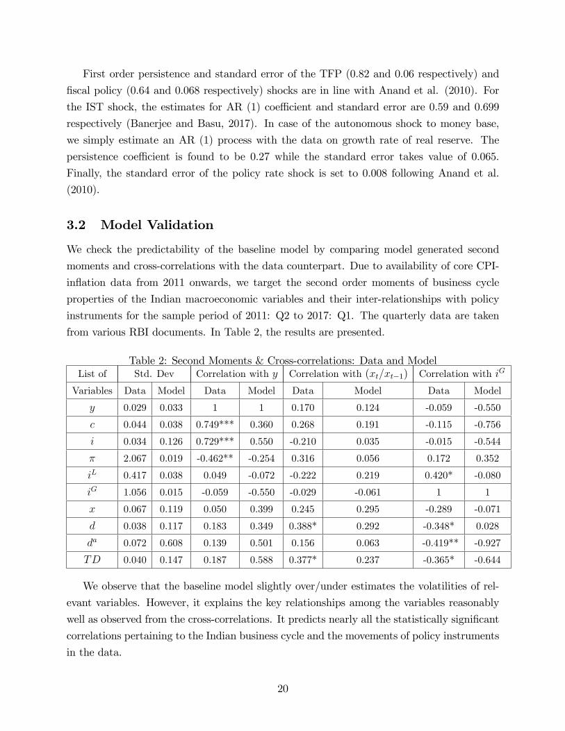
3.2 Model Validation
We check the predictability of the baseline model by comparing model generated second
moments and cross-correlations with the data counterpart. Due to availability of core CPI-
in�ation data from 2011 onwards, we target the second order moments of business cycle
properties of the Indian macroeconomic variables and their inter-relationships with policy
instruments for the sample period of 2011: Q2 to 2017: Q1. The quarterly data are taken
from various RBI documents. In Table 2, the results are presented.
Table 2: Second Moments & Cross-correlations: Data and ModelList of Std. Dev Correlation with y Correlation with (xt=xt�1) Correlation with iG
Variables Data Model Data Model Data Model Data Model
y 0.029 0.033 1 1 0.170 0.124 -0.059 -0.550
c 0.044 0.038 0.749*** 0.360 0.268 0.191 -0.115 -0.756
i 0.034 0.126 0.729*** 0.550 -0.210 0.035 -0.015 -0.544
� 2.067 0.019 -0.462** -0.254 0.316 0.056 0.172 0.352
iL 0.417 0.038 0.049 -0.072 -0.222 0.219 0.420* -0.080
iG 1.056 0.015 -0.059 -0.550 -0.029 -0.061 1 1
x 0.067 0.119 0.050 0.399 0.245 0.295 -0.289 -0.071
d 0.038 0.117 0.183 0.349 0.388* 0.292 -0.348* 0.028
da 0.072 0.608 0.139 0.501 0.156 0.063 -0.419** -0.927
TD 0.040 0.147 0.187 0.588 0.377* 0.237 -0.365* -0.644
We observe that the baseline model slightly over/under estimates the volatilities of rel-
evant variables. However, it explains the key relationships among the variables reasonably
well as observed from the cross-correlations. It predicts nearly all the statistically signi�cant
correlations pertaining to the Indian business cycle and the movements of policy instruments
in the data.
20
3.3 Impulse Response Analysis of Monetary Transmission Mech-
anism
Following the reliability check of the baseline model with data, we study the propagation
mechanism of the shocks to monetary policy instrument given that the Taylor-type stabilizer
is in place. As mentioned earlier, there are two types of policy shocks in action. First, the
shocks to base money growth which are akin to autonomous liquidity shocks and may be
beyond the control of the central bank. Second, the shocks to short-term policy interest rate
by the central bank as a conscious e¤ort to impact the real and/or �nancial target variables
according to their policy objectives. What is the propagation mechanism of such shocks to
base money and policy interest rate in the model? We investigate that using the properties
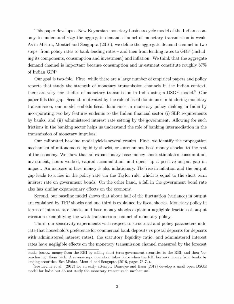
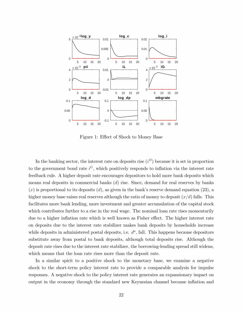
of impulse response plots given in Figure 1 and 2.
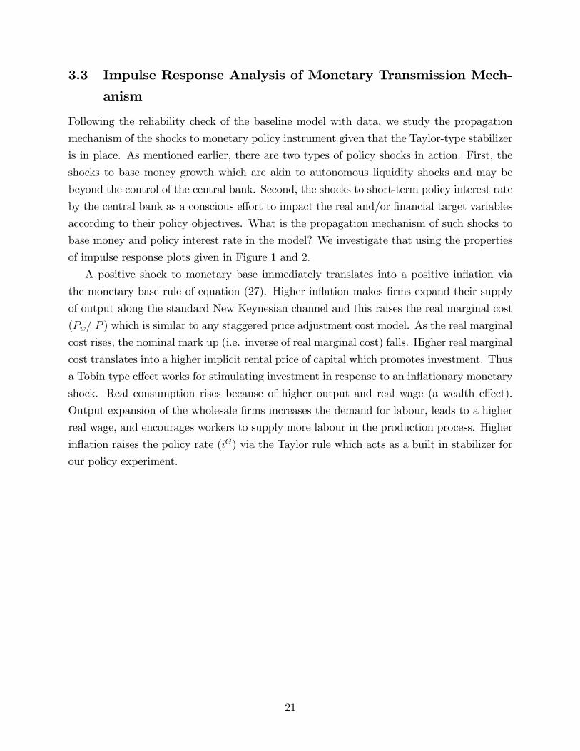
A positive shock to monetary base immediately translates into a positive in�ation via
the monetary base rule of equation (27). Higher in�ation makes �rms expand their supply
of output along the standard New Keynesian channel and this raises the real marginal cost
(Pw= P ) which is similar to any staggered price adjustment cost model. As the real marginal
cost rises, the nominal mark up (i.e. inverse of real marginal cost) falls. Higher real marginal
cost translates into a higher implicit rental price of capital which promotes investment. Thus
a Tobin type e¤ect works for stimulating investment in response to an in�ationary monetary
shock. Real consumption rises because of higher output and real wage (a wealth e¤ect).
Output expansion of the wholesale �rms increases the demand for labour, leads to a higher
real wage, and encourages workers to supply more labour in the production process. Higher
in�ation raises the policy rate (iG) via the Taylor rule which acts as a built in stabilizer for
our policy experiment.
21
5 10 15 20
10 3
0
5log_y
5 10 15 200
0.005
0.01log_c
5 10 15 200
0.01
0.02log_i
5 10 15 20
10 3
0
2
4pii
5 10 15 200.01
0
0.01iL
5 10 15 20
10 3
0
2
4iG
5 10 15 200
0.05
0.1log_d
5 10 15 200.1
0
0.1log_dp
5 10 15 200
0.05
0.1mbgrate
Figure 1: E¤ect of Shock to Money Base
In the banking sector, the interest rate on deposits rise (iD) because it is set in proportion
to the government bond rate iG, which positively responds to in�ation via the interest rate
feedback rule. A higher deposit rate encourages depositors to hold more bank deposits which
means real deposits in commercial banks (d) rise. Since, demand for real reserves by banks
(x) is proportional to its deposits (d), as given in the bank�s reserve demand equation (23), a
higher money base raises real reserves although the ratio of money to deposit (x=d) falls. This
facilitates more bank lending, more investment and greater accumulation of the capital stock
which contributes further to a rise in the real wage. The nominal loan rate rises momentarily
due to a higher in�ation rate which is well known as Fisher e¤ect. The higher interest rate
on deposits due to the interest rate stabilizer makes bank deposits by households increase
while deposits in administered postal deposits, i.e. da, fall. This happens because depositors
substitute away from postal to bank deposits, although total deposits rise. Although the
deposit rate rises due to the interest rate stabilizer, the borrowing-lending spread still widens,
which means that the loan rate rises more than the deposit rate.
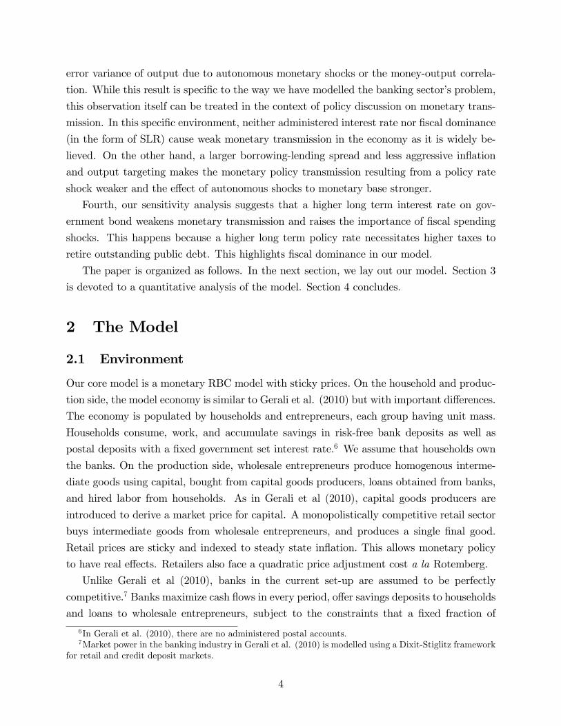
In a similar spirit to a positive shock to the monetary base, we examine a negative
shock to the short-term policy interest rate to provide a comparable analysis for impulse
responses. A negative shock to the policy interest rate generates an expansionary impact on
output in the economy through the standard new Keynesian channel because in�ation and
22
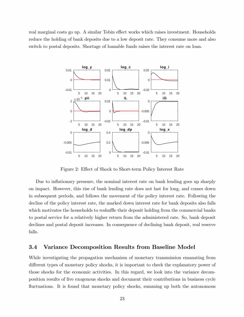
real marginal costs go up. A similar Tobin e¤ect works which raises investment. Households
reduce the holding of bank deposits due to a low deposit rate. They consume more and also
switch to postal deposits. Shortage of loanable funds raises the interest rate on loan.
5 10 15 200.01
0
0.01log_y
5 10 15 200
0.01
0.02log_c
5 10 15 200.02
0
0.02log_i
5 10 15 20
10 3
2
0
2pii
5 10 15 200.02
0
0.02iL
5 10 15 200.01
0.005
0iG
5 10 15 200.01
0.005
0log_d
5 10 15 200
0.2
0.4log_dp
5 10 15 200.01
0.005
0log_x
Figure 2: E¤ect of Shock to Short-term Policy Interest Rate
Due to in�ationary pressure, the nominal interest rate on bank lending goes up sharply
on impact. However, this rise of bank lending rate does not last for long, and comes down
in subsequent periods, and follows the movement of the policy interest rate. Following the
decline of the policy interest rate, the marked down interest rate for bank deposits also falls
which motivates the households to reshu e their deposit holding from the commercial banks
to postal service for a relatively higher return from the administered rate. So, bank deposit
declines and postal deposit increases. In consequence of declining bank deposit, real reserve
falls.
3.4 Variance Decomposition Results from Baseline Model
While investigating the propagation mechanism of monetary transmission emanating from
di¤erent types of monetary policy shocks, it is important to check the explanatory power of
those shocks for the economic activities. In this regard, we look into the variance decom-
position results of �ve exogenous shocks and document their contributions in business cycle
�uctuations. It is found that monetary policy shocks, summing up both the autonomous
23
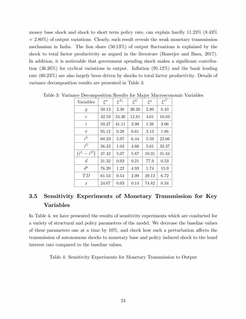
money base shock and shock to short term policy rate, can explain hardly 11.23% (8.43%
+ 2.80%) of output variations. Clearly, such result reveals the weak monetary transmission
mechanism in India. The lion share (50.13%) of output �uctuations is explained by the
shock to total factor productivity as argued in the literature (Banerjee and Basu, 2017).
In addition, it is noticeable that government spending shock makes a signi�cant contribu-
tion (36.26%) for cyclical variations in output. In�ation (95.12%) and the bank lending
rate (60.23%) are also largely been driven by shocks to total factor productivity. Details of
variance decomposition results are presented in Table 3.
Table 3: Variance Decomposition Results for Major Macroeconomic VariablesVariables �a �Zx �G �� �i
G
y 50.13 2.38 36.26 2.80 8.43
c 42.19 24.36 12.81 4.61 16.03
i 50.27 41.11 3.99 1.56 3.06
� 95.12 0.28 0.61 2.13 1.86
iL 60.23 5.07 6.44 5.59 22.66
iG 56.33 1.03 4.66 5.61 32.37�iL � iD
�47.42 5.07 5.87 10.31 31.34
d 21.32 0.03 0.21 77.9 0.53
da 76.20 1.22 4.93 1.74 15.9
TD 61.53 0.54 2.09 29.12 6.72
x 24.67 0.03 0.14 74.82 0.34
3.5 Sensitivity Experiments of Monetary Transmission for Key
Variables
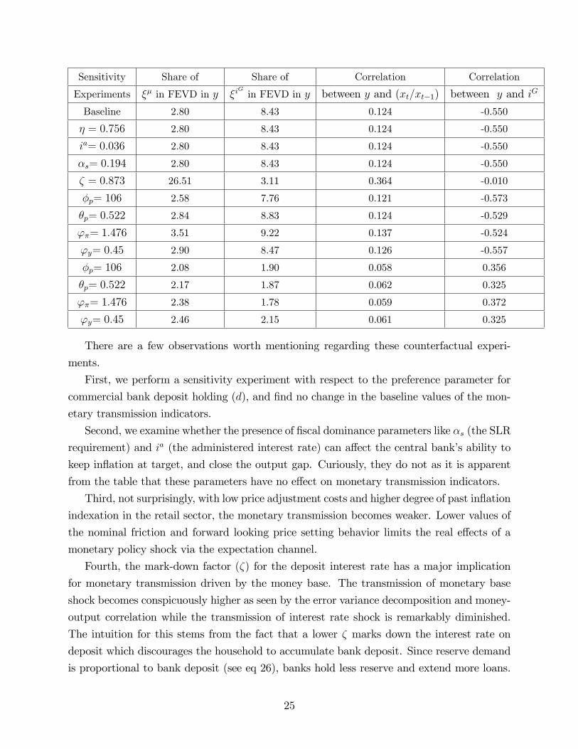
In Table 4, we have presented the results of sensitivity experiments which are conducted for
a variety of structural and policy parameters of the model. We decrease the baseline values
of these parameters one at a time by 10%, and check how such a perturbation a¤ects the
transmission of autonomous shocks to monetary base and policy induced shock to the bond
interest rate compared to the baseline values.
Table 4: Sensitivity Experiments for Monetary Transmission to Output
24
Sensitivity Share of Share of Correlation Correlation
Experiments �� in FEVD in y �iGin FEVD in y between y and (xt=xt�1) between y and iG
Baseline 2.80 8.43 0.124 -0.550
� = 0:756 2.80 8.43 0.124 -0.550
ia= 0:036 2.80 8.43 0.124 -0.550
�s= 0:194 2.80 8.43 0.124 -0.550
� = 0:873 26.51 3.11 0.364 -0.010
�p= 106 2.58 7.76 0.121 -0.573
�p= 0:522 2.84 8.83 0.124 -0.529
'�= 1:476 3.51 9.22 0.137 -0.524
'y= 0:45 2.90 8.47 0.126 -0.557
�p= 106 2.08 1.90 0.058 0.356
�p= 0:522 2.17 1.87 0.062 0.325
'�= 1:476 2.38 1.78 0.059 0.372
'y= 0:45 2.46 2.15 0.061 0.325
There are a few observations worth mentioning regarding these counterfactual experi-
ments.
First, we perform a sensitivity experiment with respect to the preference parameter for
commercial bank deposit holding (d), and �nd no change in the baseline values of the mon-
etary transmission indicators.
Second, we examine whether the presence of �scal dominance parameters like �s (the SLR
requirement) and ia (the administered interest rate) can a¤ect the central bank�s ability to
keep in�ation at target, and close the output gap. Curiously, they do not as it is apparent
from the table that these parameters have no e¤ect on monetary transmission indicators.
Third, not surprisingly, with low price adjustment costs and higher degree of past in�ation
indexation in the retail sector, the monetary transmission becomes weaker. Lower values of
the nominal friction and forward looking price setting behavior limits the real e¤ects of a
monetary policy shock via the expectation channel.
Fourth, the mark-down factor (�) for the deposit interest rate has a major implication
for monetary transmission driven by the money base. The transmission of monetary base
shock becomes conspicuously higher as seen by the error variance decomposition and money-
output correlation while the transmission of interest rate shock is remarkably diminished.
The intuition for this stems from the fact that a lower � marks down the interest rate on
deposit which discourages the household to accumulate bank deposit. Since reserve demand
is proportional to bank deposit (see eq 26), banks hold less reserve and extend more loans.
25
Thus the propagation of a shock to monetary base becomes stronger through the bank
lending channel because banks hold less reserve. On the other hand, since a lower � widens
the spread between borrowing and lending rates (iLt � iDt ), the pass through from a policy
rate shock to the bank lending rate (iLt ) becomes weaker which explains why the policy rate
accounts for less variation of output and also low correlation with output.
Finally, not surprisingly, less aggressive in�ation targeting (lower '�) and less output
stabilization (lower 'y) raises the pass through of monetary base shock to output, in�ation
and the nominal loan rate.
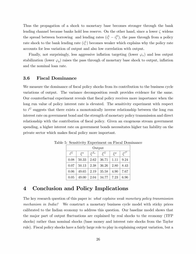
3.6 Fiscal Dominance
We measure the dominance of �scal policy shocks from its contribution to the business cycle
variations of output. The variance decomposition result provides evidence for the same.
Our counterfactual experiment reveals that �scal policy receives more importance when the
long run value of policy interest rate is elevated. The sensitivity experiment with respect
to iG suggests that there exists a monotonically inverse relationship between the long run
interest rate on government bond and the strength of monetary policy transmission and direct
relationship with the contribution of �scal policy. Given an exogenous stream government
spending, a higher interest rate on government bonds necessitates higher tax liability on the
private sector which makes �scal policy more important.
Table 5: Sensitivity Experiment on Fiscal DominanceOutput
iG �a �Zx �G �� �iG
0.08 50.33 2.62 36.71 1.11 9.24
0.07 50.13 2.38 36.26 2.80 8.43
0.06 49.65 2.19 35.58 4.90 7.67
0.05 49.00 2.04 34.77 7.23 6.96
4 Conclusion and Policy Implications
The key research question of this paper is: what explains weak monetary policy transmission
mechanism in India? We construct a monetary business cycle model with sticky prices
calibrated to the Indian economy to address this question. Our baseline model shows that
the major part of output �uctuations are explained by real shocks to the economy (TFP
shocks) rather than nominal shocks (base money and interest rate shocks from the Taylor
rule). Fiscal policy shocks have a fairly large role to play in explaining output variation, but a
26
lesser role in other macroeconomic aggregates. IST shocks have a negligible role in explaining
output �uctuations in the economy. Our estimated baseline model is also consistent with
empirical studies in the Indian context that show that while transmission to bank lending
rates is incomplete, it is still stronger than policy rate transmission to GDP, and in�ation.
Our paper also addresses a long standing hypotheses in the policy discussion on the
impediments to monetary transmission . A prominent hypothesis is that the existence of a
postal banking sector could undermine the role of monetary policy. A second hypothesis is
�scal dominance or �nancial repression. Since banks are asked to hold a fraction of deposits
as government bonds, it could weaken the e¢ cacy of monetary policy. Our estimated baseline
model does not lend support to either of these two hypotheses. The impulse response and
variance decompositions of monetary policy shock are robustly invariant to changes in the
administered postal rate, allocation of deposits between these two savings institutions, and
to changes in the statutory liquidity ratio.
The lesson is that we need to understand the instruments of monetary control better,
as well as the nature of real-monetary interactions, before we make any serious predictions
about monetary transmission. For future work, we plan to add an informal sector to the
model to understand how the presence of this a¤ects monetary transmission.
27
References
[1] Anand, Rahul, Peiris Shanaka, and Magnus Saxegaard. 2010. An Estimated Model with
Macro�nancial Linkages for India. IMF Working Paper, WP/10/21.
[2] Bernanke, Ben S., Gertler, Mark, and Simon Gilchrist. 1999. The Financial Accelerator
in a Quantitative Business Cycle Framework." In Handbook of Macroeconomics, (Eds.)
John Taylor and Michael Woodford, pp. 1341-93, Amsterdam: North Holland.
[3] Chang, Su-Hsin, Contessi, Silvio, and Johanna Francis. 2014. Understanding the accu-
mulation of bank and thrift reserves during the U.S. �nancial crisis. Journal of Economic
Dynamics and Control, Volume 43, pages 78-106.
[4] Cooley, Thomas and Gary Hansen. 1995. Money and the Business Cycle. In Frontiers
of Business Cycle Research, (Ed.) Thomas Cooley, pp. 175-216, Princeton University
Press: Princeton, New Jersey.
[5] Das, Sonali. 2015. Monetary Policy in India: Transmission to Bank Interest Rates. IMF
Working Papers 15/129, International Monetary Fund.
[6] Gerali, Andrea, Neri, Stefano, Sessa, Luca, and Frederico Signoretti. 2010. Credit and
Banking in a DSGE Model of the Euro Area. Journal of Money, Credit and Banking,
Volume, 42 (6), pages 107-141.
[7] Gabriel, Vasco, Levine, Paul, Pearlman, Joseph, and Bo Yang. 2012. An Estimated
DSGE Model of the Indian Economy. In The Oxford Handbook of the Indian Economy,
(Ed.) Chetan Ghate, pp. 835-890, Oxford University Press: New York.
[8] Mishra, Prachi, Montiel, Peter, and Rajeswari Sengupta. 2016 Monetary Transmission
in Developing Countries: Evidence from India In Monetary Policy in India: A Modern
Macroeconomic Approach (Eds.) Chetan Ghate and Ken Kletzer, pages 59-110, Springer
Verlag: New Delhi.
[9] Mohanty, Madhusudhan, and Kumar Rishabh. 2016. Financial Intermediation and Mon-
etary Policy Transmission in EMEs: What has Changed since the 2008 Crisis ?. In
Monetary Policy in India: A Modern Macroeconomic Approach (Eds.) Chetan Ghate
and Ken Kletzer, pages 111-150, Springer Verlag: New Delhi.
[10] Sahu, Jagadish Prasad. 2013. In�ation Dynamics in India. A Hybrid New Keynesian
Approach. Economics Bulletin, Volume 33 (4), pp. 2634-2647
28

[11] Urjit Patel Committee Report. 2014.
29
5 Technical Appendix A
� The Lagrangian for the household problem is given by,
Lt = Et
1Xt=0
�t[U(Ct)� �(Ht) + V (Dt=Pt; Dat =Pt)� (42)
�t(PtCt + PtTt +Dt +Dat �WtHt �
�1 + iDt
�Dt�1 � (1 + ia)Da
t�1 � �kt � �rt � �bt)]
The household�s optimal choices are given by
@Lt@Ct
= U 0(Ct)� �tPt = 0
@Lt@Ht
= �0(Ht)� �tWt = 0
@Lt@Dt
=V1(Dt=Pt; D
at =Pt)
Pt� �t + ��t+1
�1 + iDt+1
�= 0
@Lt@Da
t
=V2(Dt=Pt; D
at =Pt)
Pt� �t + ��t+1 (1 + ia) = 0:
� To obtain equation (9), set t;t = 1 in (8), and solve for Qt,
0 = PtQt � Pt�1 + S
�ItIt�1
��� PtS 0
�ItIt�1
�ItIt�1
+ t;t+1Pt+1S0�It+1It
��It+1It
�2PtQt = Pt
�1 + S
�ItIt�1
��+ PtS
0�ItIt�1
�ItIt�1
� t;t+1Pt+1S 0�It+1It
��It+1It
�2Qt =
�1 + S
�ItIt�1
��+ S 0
�ItIt�1
�ItIt�1
� t;t+1Pt+1PtS 0�It+1It
��It+1It
�2Note that t;t+1 = �Et [U 0 (Ct+1) =U 0 (Ct)] [Pt=Pt+1]. Substituting this, we get equation
(9)
� To derive equation (23), the Lagrangian is given by
Et
1Xs=0
t;t+s
8>>>><>>>>:
264 (1 + iLt )Lt�1 + (1 + i
R)MRt�1 � (� � �s)(1 + iGt )Dt�1
�(1 + ip)Emax(]Wt�1 �MRt�1; 0)
+(1� �s)Dt � Lt �MRt
375+�t
�MRt � �rDt
�
9>>>>=>>>>;30
which is equivalent to
Et
1Xs=0
t;t+s
8>>>><>>>>:
2664(1 + iLt )Lt�1 + (1 + i
R)MRt�1 � (� � �s)(1 + iGt )Dt�1
�(1 + ip)R Dt�1MRt�1
h]Wt�1 �MR
t�1
if(]Wt�1)dWt�1
+(1� �s)Dt � Lt �MRt
3775+�t
�MRt � �rDt
�
9>>>>=>>>>; :
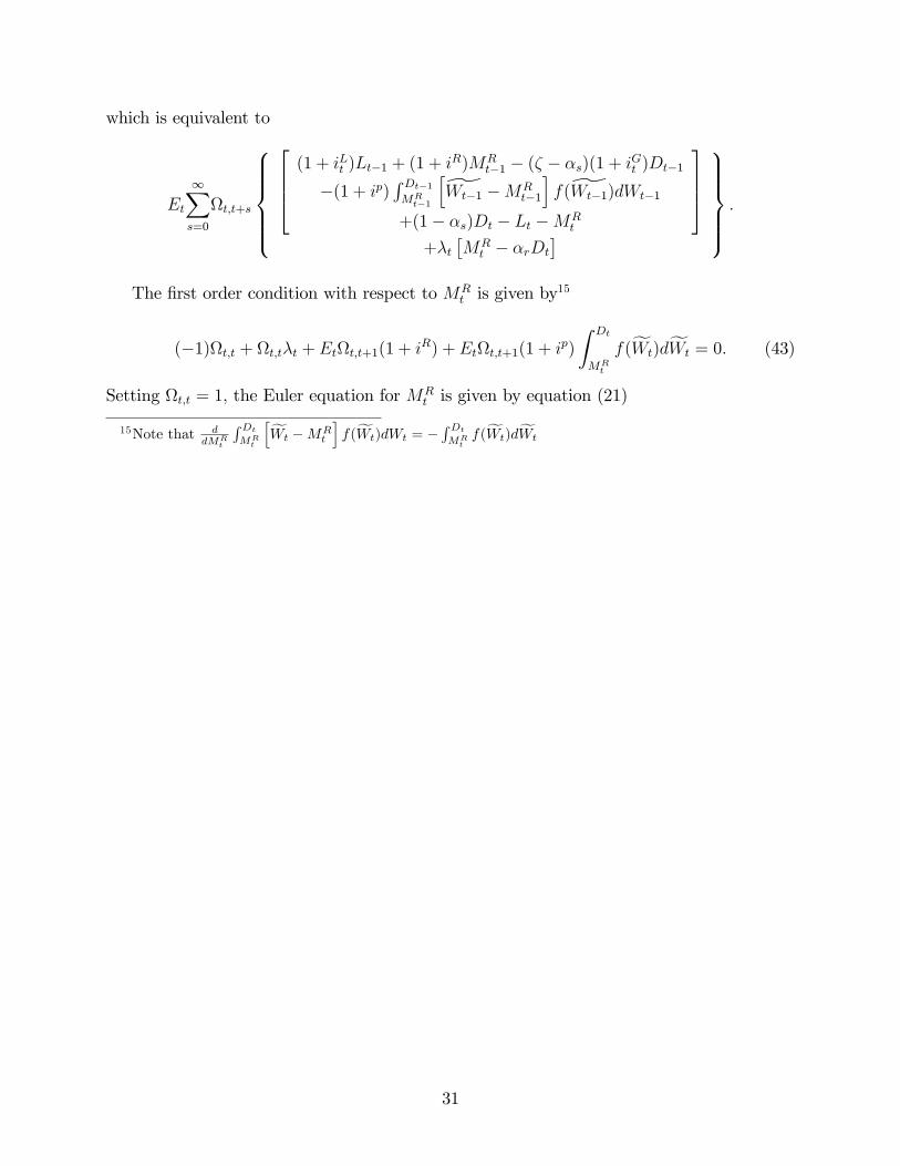
The �rst order condition with respect to MRt is given by
15
(�1)t;t + t;t�t + Ett;t+1(1 + iR) + Ett;t+1(1 + ip)Z Dt
MRt
f(fWt)dfWt = 0: (43)
Setting t;t = 1; the Euler equation for MRt is given by equation (21)
15Note that ddMR
t
RDt
MRt
hfWt �MRt
if(fWt)dWt = �
RDt
MRtf(fWt)dfWt
31
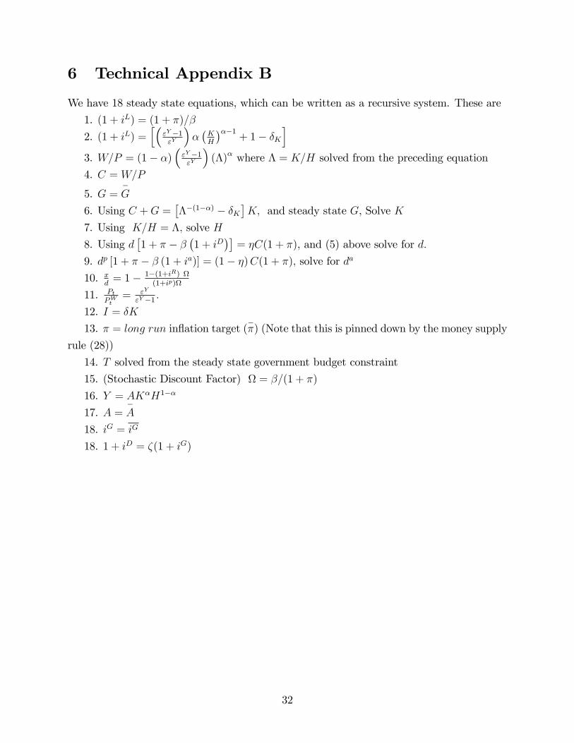
6 Technical Appendix B
We have 18 steady state equations, which can be written as a recursive system. These are
1. (1 + iL) = (1 + �)=�
2. (1 + iL) =h�
"Y �1"Y
���KH
���1+ 1� �K
i3. W=P = (1� �)
�"Y �1"Y
�(�)� where � = K=H solved from the preceding equation
4. C = W=P
5. G =�G
6. Using C +G =���(1��) � �K
�K; and steady state G, Solve K
7. Using K=H = �; solve H
8. Using d�1 + � � �
�1 + iD
��= �C(1 + �), and (5) above solve for d:
9. dp [1 + � � � (1 + ia)] = (1� �)C(1 + �); solve for da
10. xd= 1� 1�(1+iR)
(1+ip)
11. PtPWt
= "Y
"Y �1 :
12. I = �K
13. � = long run in�ation target (��) (Note that this is pinned down by the money supply
rule (28))
14. T solved from the steady state government budget constraint
15. (Stochastic Discount Factor) = �=(1 + �)
16. Y = AK�H1��
17. A =�A
18. iG = iG
18. 1 + iD = �(1 + iG)
32
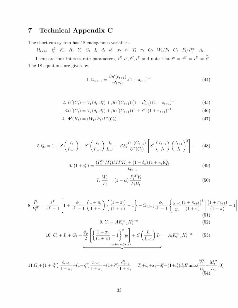
7 Technical Appendix C
The short run system has 18 endogenous variables:
t;t+1 iLt Kt Ht Yt Ct It dt dpt xt ipt Tt �t Qt Wt=Pt Gt Pt=Pwt At :
There are four interest rate parameters, iR; ia; iG; iD;and note that ia = iG = iD =�is:
The 18 equations are given by.
1: t;t+1 =�u0(ct+1)
u0(ct):(1 + �t+1)
�1 (44)
2. U 0(Ct) = V0
1 (dt; dat ) + �U
0(Ct+1)�1 + iDt+1
�(1 + �t+1)
�1 (45)
3:U 0(Ct) = V0
2 (dt; dat ) + �U
0(Ct+1) (1 + ia) (1 + �t+1)
�1 (46)
4. �0(Ht) = (Wt=Pt)U0(Ct): (47)
5:Qt = 1 + S
�ItIt�1
�+ S 0
�ItIt�1
�ItIt�1
� �EtU 0 (Ct+1)
U 0 (Ct)
"S 0�It+1It
��It+1It
�2#: (48)
6: (1 + iLt ) =(PWt =Pt)MPKt + (1� �k) (1 + �t)Qt
Qt�1(49)
7:Wt
Pt= (1� �) P
Wt YtPtHt
(50)
8:PtPWt
="Y
"Y � 1
"1 +
�p"Y � 1
�1 + �t1 + �
��(1 + �t)
(1 + �)� 1�� t;t+1
�p"Y � 1
(yt+1yt
(1 + �t+1)2
(1 + �)
�(1 + �t+1)
(1 + �)� 1�)#�1
(51)
9: Yt = AK�t�1H
1��t (52)
10: Ct + It +Gt +�p2
"�1 + �t(1 + �)
� 1�2yt
#+ S
�ItIt�1
�It
price adj cos t| {z }= AtK
�t�1H
1��t (53)
11:Gt+�1 + iGt
� bt�11 + �t
+(1+iRt )xt�11 + �t
+(1+ia)dat�11 + �t
= Tt+bt+xt+dat+(1+i
pt )dtEmax(
fWt
Dt
�MRt
Dt
; 0)
(54)
33
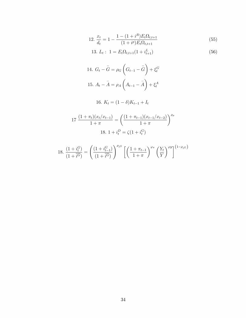
12:xtdt= 1� 1� (1 + i
R)Ett;t+1(1 + ip)Ett;t+1
(55)
13: Lt : 1 = Ett;t+1(1 + iLt+1) (56)
14. Gt ��G = �G
�Gt�1 �
�G
�+ �Gt
15: At ��A = �A
�At�1 �
�A
�+ �At
16: Kt = (1� �)Kt�1 + It
17(1 + �t)(xt=xt�1)
1 + �=
�(1 + �t�1)(xt�1=xt�2)
1 + �
���18: 1 + iDt = �(1 + i
Gt )
18:(1 + iGt )
(1 + iG)=
(1 + iGt�1)
(1 + iG)
!�iG ��
1 + �t�11 + �
�'� �YtY
�'y�(1��iG)
34
Related Documents