A MODIFIED METHOD FOR BAYESIAN …eprints.usm.my/32266/1/ALMUTAIRI_ANED_OMAR.pdfA MODIFIED METHOD FOR BAYESIAN PREDICTION OF FUTURE ORDER STATISTICS FROM GENERALIZED POWER FUNCTION

A MODIFIED METHOD FOR BAYESIAN

PREDICTION OF FUTURE ORDER STATISTICS

FROM GENERALIZED POWER FUNCTION

ALMUTAIRI ANED OMAR

UNIVERSITI SAINS MALAYSIA

2015

A MODIFIED METHOD FOR BAYESIAN PREDICTION OF FUTURE

ORDER STATISTICS FROM GENERALIZED POWER FUNCTION

By

ALMUTAIRI ANED OMAR

Thesis Submitted in Fulfillment of the Requirements for the Degree of Doctor

of Philosophy

April 2015

i

ii

ACKNOWLEDGEMENTS

I would like to take this opportunity to express my deep gratitude to those who have

contributed throughout the duration of my research work. First and foremost, I would

like to extend my gratitude to my supervisor, Professor Dr. Low Heng Chin, for her

guidance, invaluable advice and continuous concern throughout this thesis. Sincere

thanks to the Dean of the School of Mathematical Sciences and the staff in Universiti

Sains Malaysia especially the staff in the School of Mathematical Sciences for their

assistance and cooperation. Finally, I would like to thank all my family members, my

colleagues and friends for their support and sharing. Last but not least, my sincere

thanks and appreciation to my father, my mother and my sister for their

encouragement, understanding and support throughout the period spent in

completing this thesis.

iii

TABLE OF CONTENTS

Page

ACKNOWLEDGEMENTS ii

TABLE OF CONTENTS iii

LIST OF TABLES ix

LIST OF FIGURES x

LIST OF SYMBOLS

LIST OF ABBREVIATIONS

xi

xv

LIST OF PUBLICATIONS xvi

ABSTRAK xvii

ABSTRACT

xix

CHAPTER

1 INTRODUCTION

1.1 Background of the study 1

1.1.1 Future sample and present sample 1

1.1.2 Order statistics 4

1.1.3 Aging 5

1.1.4 Bayesian statistic 8

1.1.4.1 Prior distributions 11

1.1.4.2 Posterior distributions 13

1.1.4.3 The Bayes risk function 14

1.1.5 Bayesian prediction 16

1.1.5.1 Types of Bayesian prediction. . .

. . . . . problems

16

iv

1.1.5.2 Bayesian prediction intervals 17

1.2 Problem identification and the importance of the

study

18

1.3 Objectives of the study 19

1.4 Organization of thesis 19

2 LITERATURE REVIEW

2.1 Introduction 21

2.2 Pearson’s System 21

2.2.1 Different forms of the probability density

. . function for the generalized power

…. function distribution

23

2.3 Bayesian prediction intervals of future order

statistics

28

2.4

2.5

2.6

2.7

2.8

Predictive distribution of a single future response

Bayesian estimation of parameters for some life

distributions

Bayesian estimation by squared-error loss

function

Monte Carlo simulation study

Summary

33

38

39

40

43

v

3 A MODIFIED METHOD FOR BAYESIAN PREDICTION OF

FUTURE ORDER STATISTICS FROM GENERALIZED

POWER FUNCTION

3.1 Introduction 45

3.2 A modified method for Bayesian prediction 45

3.2.1 Bayesian prediction interval for the ℎ order

. . . statistic: two samples case

45

3.2.1.1 Posterior distribution for informative

. prior: two samples case

46

3.2.1.2 Posterior distribution for non-

. . . . . . . . informative prior: two samples case

48

3.2.1.3 Predictive density function for the

. . . ℎ order statistic: two samples case

49

3.2.1.4 Bayesian prediction bound of k 53

3.2.1.5 Special cases for Bayesian prediction

. . . . . . interval of �

55

3.2.2 Bayesian prediction . interval . . for. . . the

. + ℎ order statistic: one sample case

59

3.2.2.1 Predictive . . density . . function of

. + : one sample case

60

3.2.2.2 Bayesian prediction bound of + 63

3.2.2.3 Special cases for Bayesian

. . . . . . . . . prediction interval +

65

vi

3.2.3 Bayesian prediction interval for the ℎ order

. statistic: multi samples case

67

3.2.3.1 Posterior distribution for

. . . . . . . informative prior function: multi

. . . samples case

68

3.2.3.2 Posterior distribution for non-.

. . . . . . informative prior function: multi

. . . samples case

68

3.2.3.3 Predictive density function for the

. . . . ℎorder statistic: multi samples case

69

3.2.3.4 Bayesian prediction bound of S 71

3.2.3.5 Special cases for Bayesian prediction

. . . . . interval of S

73

3.3 Summary 76

4 BAYESIAN ESTIMATION OF PARAMETERS FROM

GENERALIZED POWER FUNCTION DISTRIBUTION

4.1 Introduction 77

4.2 Bayesian estimate for shape parameter 77

4.2.1 Case of non-informative prior distribution and

. . . . squared error loss function

78

4.2.2 Case of informative prior distribution and

. . . . . . squared error loss function

80

4.3

Bayesian estimate for scale parameter 81

vii

4.4

4.3.1 Case of non-informative prior distribution

. . and squared error loss function

Summary

81

83

5 NUMERICAL ANALYSIS

5.1... Introduction 85

5.2 …

Numerical examples on Bayesian prediction intervals

for the ℎorder statistic: two samples case

85

5.3 .

5.4 .

Numerical examples on Bayesian prediction intervals

for.the + ℎ order statistic (one sample case) and

.. ℎorder statistic (multi samples case)

Numerical examples on Bayesian estimate

90

95

6 CONCLUSION

6.1 ... Introduction 104

6.2 …

6.3 …

Summary

Contributions

104

105

6.4 … Future Research 107

REFERENCES 108

viii

APPENDICES

APPENDIX A

APPENDIX B

A FORTRAN program for Bayesian prediction

interval of.one, two and multi samples

A FORTRAN program for Bayesian estimation of

shape, scale and location parameters

113

119

ix

LIST OF TABLES

Page

2 Survival times (weeks) of 20 carcinoma patients medical diagnosis 1.1

22 Phases of the Pearson’s system 2.1

41 Means and MSEs (in parentheses) of the estimates of St for

different values of & � = .5

2.2

42

87

Means and MSEs (in parentheses) of the estimates of St for

different values of and � =

Observations from a present sample

2.3

5.1

88 95% Bayesian prediction intervals: two samples 5.2

89 99% Bayesian prediction intervals: two samples 5.3

91 95% Bayesian prediction intervals: one sample 5.4

91 99% Bayesian prediction intervals: one sample 5.5

93

94

95% Bayesian prediction intervals: multi samples

99% Bayesian prediction intervals: multi samples

5.6

5.7

98

Bayesian estimator � for shape parameter by use of

non-informative prior

5.8

100

Bayesian estimator � for shape parameter � by use of

informative prior

5.9

103 Bayesian estimate for scale paramete 5.10

x

LIST OF FIGURES

Page

7 Curve of the failure rate function 1.1

24 Probability density functions for the standard generalized

power function distribution with a known scale

parameter =

2.1

27 Probability density functions for the generalized power

function distribution of Equation (2.4)

2.2

27 Reliability functions for the generalized power function

distribution of Equation (2.10)

2.3

27 Failure rate functions for the generalized power function 2.4

distribution of Equation (2.12)

xi

LIST OF SYMBOLS

location parameter of standard generalized power function

scale parameter of standard generalized power function

, parameters of informative prior function

decision function

Bayes estimator

∗ Bayesian decision function

�| mean of the posterior distribution for �

| mean posterior function for

informative experiment

future experiment

probability density function

cumulative distribution function

, ℎ parameters of informative prior function

Group � action space

Group � parameter space

Group � space of

Group decision space

xii

�| posterior distribution for informative prior function

�| posterior distribution for non-informative prior function

�| posterior distribution of informative prior function for multi sample

�| posterior distribution of non-informative prior function for multi

sample

�| posterior distribution for non- informative prior function

�| posterior distribution for informative prior function

ℎ failure rate function

ℎ � prior density function

sufficient statistic for � and multi samples prediction

� complete sufficient statistic for � and the complete sample

� lower limit for Bayesian prediction interval

� likelihood function

�, squared error loss function

size of future sample

� shape parameter of standard generalized power function

� �| predictive density function of �

� + | predictive density function of +

xiii

� | predictive density function of

�, risk function

Bayesian risk

Reliability distribution function

survival function of pareto distribution

∗ Bayesian estimator of

complete sufficient statistic for � and one-two sample prediction

upper limit for Bayesian prediction interval

sufficient statistic for � and one-two sample prediction

� ℎ order statistic from the future sample for two samples

prediction

ℎ order statistic from the future sample for one sample prediction

the first order statistic

� the order statistic

� the order statistic � , + interval of failure rate function

� future response from two-parameter exponential distribution

+ + ℎ order statistic of future sample for one sample prediction

xiv

− confidence prediction coefficient

� location parameter of two-parameter exponential distribution

� scale parameter of two-parameter exponential distribution

complete sufficient statistic for � and multi samples prediction

sufficient statistic for � and the complete sample

Bayesian estimator of

� Bayesian estimator of � for non-informative prior function

� Bayesian estimator of � for informative prior function

Bayesian estimator of

xv

LIST OF ABBREVIATIONS

� cumulative density function

CFR constant failure rate

DFR decreasing failure rate

IFR increasing failure rate

LINEX linear exponential loss function

MMAE minimum mean absolute error

MMSE minimum mean squared error

PD highest predictive density

� probability density function

xvi

LIST OF PUBLICATIONS

1. Al Mutairi Aned O. and Heng Chin Low, Bayesian Estimate for Shape

Parameter from Generalized Power Function Distribution, Journal of

Mathematical Theory and Modeling. (2012), Vol.2, No.12, ISSN 2224-5804

(Paper) ISSN 2225-0522 (Online).

2. Al Mutairi Aned O. and Heng Chin Low, Bayesian Estimates of Parameters

for Life Distributions based on Different Loss Functions, Advances in Applied

Mathematical Analysis Journal. (2013), Vol. 8 Number 1, ISSN 0973-5313

p.11-17.

3. Al Mutairi Aned O. and Heng Chin Low, Concepts in Order Statistics and

Bayesian Estimation, Journal of Mathematical Theory and Modeling. (2013),

Vol.3, No.4, ISSN 2224-5804 (Paper) ISSN 2225-0522 (Online).

xvii

SATU KAEDAH DIUBAHSUAI UNTUK RAMALAN BAYESIAN BAGI

STATISTIK TERTIB MASA DEPAN DARIPADA FUNGSI KUASA

TERITLAK

ABSTRAK

Statistik Bayesian adalah kaedah statistik yang digunakan secara meluas dalam

pelbagai bidang seperti perubatan, sains sosial dan ekonomi. Ramalan Bayesian

adalah salah satu kaedah statistik Bayesian. Ia bekerja dengan pelbagai kaedah.

Kajian ini turut membincangkan tiga kaedah ramalan Bayesian. Terdapat satu

sampel, dua sampel dan sampel pelbagai ramalan. Tiga kaedah bertindak balas

terhadap motivasi praktikal yang memerlukan data sampel kurang, dalam

kebanyakan kajian statistik digunakan. Oleh itu, sampel yang akan datang adalah

istilah yang penting dalam tesis ini. Pendekatan Bayesian menggunakan ramalan

untuk statistik tertib masa depan berdasarkan data tertib yang diperhatikan dan fungsi

ketumpatan ramalan memberi selang ramalan Bayesian untuk statistik tertib masa

depan. Taburan fungsi kuasa teritlak piawai adalah dasar untuk tiga kaedah dengan

menggunakan teori Bayes untuk mencapai had rendah dan had atas yang sempit bagi

selang ramalan Bayesian 95% dan selang ramalan Bayesian 99%. Selang yang

dicadangkan menyumbang dalam peningkatan ketepatan untuk nilai ramalan.

Prestasi tiga kaedah dinilai oleh had rendah dan had atas dari sampel yang

diperhatikan dan untuk statistik tertib dari sampel masa depan. Dua jenis fungsi

priori digunakan dalam ramalan Bayesian: prior bermaklumat dan prior bukan

bermaklumat. Analisis berangka menunjukkan had rendah dan had atas bagi selang

xviii

ramalan Bayesian 95% dan selang ramalan Bayesian 99% untuk tiga kaedah, dan set

data dihasilkan daripada taburan fungsi kuasa teritlak piawai.

Anggaran Bayesian digunakan untuk parameter bentuk, parameter skala dan

parameter lokasi. Penganggar Bayesian dicadangkan sebagai min taburan posterior

berdasarkan fungsi prior bermaklumat atau fungsi prior bukan bermaklumat. Kedua-

dua fungsi prior menggunakan rumus bagi taburan posterior dari teori Bayes untuk

menggabungkan fungsi kebolehjadian dan fungsi prior. Penganggar Bayesian yang

dicadangkan ialah min taburan posterior berdasarkan taburan fungsi kuasa teritlak

piawai dan fungsi kehilangan ralat kuasa dua. Selain teknik ini, kriteria Bayesian

digunakan. Prestasi penganggar bentuk, skala dan lokasi dinilai oleh beberapa jenis

taburan prior dan digunakan dalam masa yang sama dengan ramalan Bayesian, yang

jika dibandingkan, mengesahkan kewajaran dan kelebihan dari beberapa jenis

taburan prior untuk anggaran atau ramalan menggunakan kaedah Bayesian. Analisis

berangka menunjukkan penganggar yang dicadangkan oleh set data yang dihasilkan

daripada taburan fungsi kuasa teritlak piawai.

xix

A MODIFIED METHOD FOR BAYESIAN PREDICTION OF FUTURE

ORDER STATISTICS FROM GENERALIZED POWER FUNCTION

ABSTRACT

Bayesian statistics is a statistical method that is widely used in many fields, including

medicine, social and applied sciences. These fields occasionally have little or limited

information about their populations. Therefore, using new techniques that require

fewer samples while providing the same quality as the case of available samples is

necessary. Bayesian prediction is a commonly used tool in Bayesian statistics. This

study modifies three Bayesian prediction methods: one-, two- and multi-sample

predictions. Bayesian prediction modified method does not require the many

samples. Therefore, a future sample is a significant term in this thesis. Our Bayesian

prediction modified method used a prediction for the future order statistics based on

the observed ordered data, and predictive densities provided the Bayesian prediction

intervals for the future order statistics. The standard generalized power function

distribution serves as the basis for the three modified methods by applying Bayes'

theory to achieve close lower and upper limits for the 95% and 99% Bayesian

prediction intervals. The proposed intervals contributed to increasing the precision

for the predictive value. The performance of the three modified methods is evaluated

using the lower and upper limits from the observed sample and for the order statistic

from the future sample. Two types of prior functions are used in Bayesian prediction:

informative and non-informative priors, both of which use Bayes' theory. The

numerical analysis illustrates lower and upper limits for the 95% and 99% Bayesian

xx

prediction intervals for the three modified methods, and the data set generated from

the standard generalized power function distribution. Bayesian estimation is used to

determine the shape, scale and location parameters. Bayesian estimators are

suggested as the mean of the posterior distribution based on an informative or non-

informative prior function. Both prior functions use a formula for the posterior

distribution from Bayes theory to combine the likelihood function and prior function.

The proposed Bayesian estimator is the mean of the posterior distribution based on

the standard generalized power function distribution and a squared error loss

function. In addition to this technique, a Bayesian criterion is used. The performance

of the shape, scale and location estimators are evaluated with some types of prior

distributions and used simultaneously with the Bayesian prediction, which, when

compared, confirms the suitability and advantage of some types of prior distributions

for estimation or prediction using the Bayesian method. The numerical analysis

illustrates the proposed estimators derived from the data set generated from the

standard generalized power function distribution.

1

CHAPTER 1

INTRODUCTION

1.1 Background of the study

The Reliability distribution function analysis is used for estimation and

prediction. It was formulated during the early research in the science of insurance,

life schedules and mortality. Modern analysis of the reliability distribution

began approximately 50 years ago in engineering applications. The incentives to

study this probability function increased in World War II when studying the failure

rates of war machines led to a marked improvement in them. After World War II, the

progress made in increasing the lifetimes of war machines was used for machines in

civil applications. Researchers initially focused on the parametric approach for

random variables that follow a known distribution, such as the normal, exponential,

Weibull or gamma distributions; thereafter, they focused on the prediction and

testing of hypotheses for parameters of these distributions. When interest of the

prediction and testing of hypotheses in medical and biological research increased, so

did interest in using a non-parametric approach. Both non-parametric and parametric

approaches concerning positive random variables are used in estimation and

prediction.

1.1.1 Future sample and present sample

Statistical inference from a Bayesian perspective usually requires less sample data to

achieve the same quality of inference compared with sampling theory-based

2

methods. In many cases, this is the practical motivation for using a future sample.

Aitchison and Dunsmore (1975) presented a medical example to explain the concept

of future sample.

Example 1.1

Table 1.1. Survival times (weeks) of 20 carcinoma patients medical diagnosis

25 45 238 194 16 23 30 16 22 123

51 412 45 162 14 72 5 35 30 91

The data in Table 1.1 are the survival times (weeks) of 20 patients suffering from

a certain type of carcinoma and receiving treatment of preoperative radiotherapy

followed by radical surgery. On the basis of this information, what can appropriately

be said about the future of a new patient with this type of carcinoma and assigned to

this form of treatment? Clearly any rational statement would regard 100 weeks

survival as much more plausible than 500 weeks survival, but how should such views

be summarized and quantified? What is a reasonable assessment of the probability

that the patient will survive 100 weeks?

In this example the informative experiment consists of recording the survival times

of the 20 patients already treated. The future experiment consists of treating a new

patient similarly and recording his survival time. If no change in the treatment has

been made since conducting , then and consist of 20 replicates and a single

replicate of the same basic trial (record the survival time of a treated patient),

respectively and are independent.

Attempts to quantify medical prognoses are of vital importance when similar

information on an alternative treatment, for example, radical surgery followed by

3

postoperative radiotherapy, is available and a choice has to be made between

treatments for a particular patient.

In life testing, it is possible to predict age of survival of observations or age of

survival for all systems because we have the sample space, random variables and

distribution functions. But sometimes the information of the experiment is not

complete. Therefore, there is a necessity to use new methods that provide some new

information, especially when the sample is not found.

Bayesian prediction can treat the problem of absent sample (future sample) by using

the present sample and can assume some assumptions which relate between random

variable from present sample and random variable � from future sample as an

interval which is given as follows: (� < � < ) = − , .

where � is the lower prediction bound and is the upper prediction bound

from the present sample. � , is a − % Bayesian prediction interval for a future random

variable � if − is called the confidence prediction coefficient (Alamm et al.,

2007). However, Gianola and Fernando (1986) presented the concept of − α % Bayesian confidence interval from Bayesian prediction interval which

plays an essential role in the posterior function if we have the following:

� ∈ | = ∫ �| �, .

4

where is a region of the space of parameter �. Fixing the probability in Equation

(1.2) at say − α , for a given , it is possible to obtain an interval for � such that

its probability content is − α .

When we choose a specific distribution, we can obtain estimates of parameters or

Bayesian prediction intervals. Kamps (1995) and Kamps and Gather (1997)

introduced the concept of generalized order statistics as a unified approach to various

ordered random variable models, such as last order statistics, sequential order

statistics, and last observed values. After that emerged the concept of censoring

schemes. Many authors have used censored order statistics in their works (Burkschat

et al., 2006, Howlader and Hossain, 2002). In addition, Soliman (2000) used the

order statistics censoring with Rayleigh distribution and presented its estimators.

Then the researchers started thinking about future order statistics as Fernandez

(2000a) and Alamm et al. (2007).

1.1.2 Order statistics

Order statistics have a major role in statistical inference, especially in laboratory

methods. If � = � , � , … , � is a random sample selected from a population, then

the probability density function is and its cumulative distribution function

is . If we arrange these observations in increasing order, we obtain the

following: � < � < ⋯ < � < ⋯ < � .

where � is the smallest observation and is called the first order statistic, � is the largest observation and is called the ℎ order statistic,

and � is the ℎ order observation and is called the ℎ order statistic.

5

Thus, � , � , … , � are the order statistics and they yield the probability density

function for the order statistics as follows:

= !− ! − ! [ ] − [ − ] − .

If = , the probability density function for the (smallest) first observation is = [ − ] − .

However, if = , the probability density function for the largest observation is = [ ] − .

(Hogg and Craig, 2013).

1.1.3 Aging

The concept of aging is a basic concept in statistics, especially in reliability, and it

has many applications in engineering, physics, and biology. Aging has three types:

i. Positive aging with time, where the unit age reduces with the progress of

time. Over time, this type of aging may lead to the erosion of industrial units,

which requires plans for maintenance or replacement. In addition, the passage

of time may result in living organisms, including humans reaching old age,

and this possibility requires the development of plans for remediation.

ii. Fixed aging, which is not affected by time. An example of fixed aging is

electronic industrial units that follow the exponential model of a failure rate

that is fixed in time.

iii. Negative aging with time, which leads to the improvement of an industrial

unit after the beginning of the operation of new units. In that case, the proper

units will remain and defective units will fail at the beginning of their

industrial operation. As for the biological side, children who are healthy at

6

birth live and become stronger over time, whereas unhealthy children die

after birth (Hendi and Sultan, 2004).

Some basic functions that accompany aging are defined as follows:

Definition 1.1

If � is a positive random variable, the reliability distribution function after age � is defined as follows: = = − = � > .

Definition 1.2

If � is a positive random variable, then the cumulative distribution is defined

as: = � .

Definition 1.3

If � is a positive random variable, the probability density function is defined as

= .

(Hogg and Craig, 2013).

Definition 1.4

If � is a positive random variable, the failure rate function ℎ � during the

interval , + is defined as:

ℎ � = → < � < + |� > = , � > .

The failure rate function, ℎ � , has three important cases in all applications (whether

engineering or biological) through the following Equation:

7

ℎ � = � − + − � − � � � , �, , , > , , � > .

The previous Equation (1.11) takes a -shaped curve with the �-axis of time as

follows:

Figure 1.1. Curve of the failure rate function

From Figure 1.1, the curve of the failure rate function is described in ℎ � by

Equation (1.11).

i. The first part, DFR, of the -shaped curve indicates that the failure rate

function, ℎ � , is decreasing with time �. This process is symbolized by the

Decreasing Failure Rate (DFR), as the value of the failure rate function, ℎ � , is high at the beginning of the operation of industrial units because of

the presence of manufacturing defects in raw materials, machines, workers,

DFR CFR IFR

Y

ℎ �

8

the quality of production, or in terms of biology (including human) because

of the presence of birth defects after birth.

ii. The second part, CFR, of the -shaped curve of the failure rate function, ℎ � , is a constant function over time � and is equal to a fixed amount ,

which is not affected by time and is symbolized by the Constant Failure Rate

(CFR) and explained practically by uncontrolled reasons. Uncontrolled

reasons include accidents representing sudden high-voltage power in the

electricity source that is due to a default in the main power station; such

accidents result in the destruction of houses or infant mortality, which can

occur when infants drink poisonous substances that are intended for cleaning

or chase a ball into a street in front of a speeding car.

iii. The third part, IFR, of the -shaped curve shows that the failure rate

function, ℎ � , is increasing over time �, which is symbolized by the

Increasing Failure Rate (IFR). Indeed, the value of the failure rate function, ℎ � , is small at the beginning with respect to time �, and then, this function

increases over time. This phenomenon is explained practically for reasons of

aging, antiquity, and corrosion of industrial machines or in terms of

biological (including human) factors for reasons of aging (Hendi and Sultan,

2004).

1.1.4 Bayesian statistic

In some statistical applications, it is preferred to use statistical inferences from the

perspective of decision science through the study of loss associated with the

sequence of possible decisions, e.g., patterns of decision of a buyer, investor, or

institution.

9

The formulation of decision-making using a probabilistic model requires a

mathematical structure in a general form. Bayesian statistical inferences and the

corresponding mathematical structure are formulated as follows:

a) Group represents action space where contains every method

possible � .

b) Group Θ represents parameter space where Θ contains every level possible � ∈ Θ.

c) Group is a partial group from real numbers set representing space of �

for every value � = to ensure ∈ ; thus, has probability density

function related to the distribution family { , � ; � ∈ Θ}.

d) Group represents the decision space and contains every possible decision � . (Hendi and Sultan, 2004)

The decision maker, when choosing the action , should note some connotations

from the population that provide him with information on the unknown parameter �.

Furthermore, the decision maker studies the random variable �, where � = and is a real value from , as well as the probability density function of the random

variable �, namely, , � , which provides him with some guidance on the

parameter � that will assist him in the selection of the action . Decision theory

focuses on the properties and methods that demonstrate how to make such a choice.

The parameter �, where � ∈ Θ, is found in nature without any intervention from the

decision maker and without any knowledge of its value having been estimated by the

decision maker with the action ∈ . A loss arises from this estimation, and the

10

loss’s function is denoted by the symbol �, . It is appropriate for the decision

maker to choose the random variable, �, which has a density function , � , to

provide him with some information about the nature of � ∈ Θ. The selection of the

decision function represents the plan followed by the decision maker in

determining this nature.

The Bayesian estimate and tests of hypotheses are only special cases of issues of

public decisions. In the Bayesian estimate, we set = Θ (in some cases, it is the real

number set or an interval from it). The required step is to select the appropriate value

for the parameter �.

(Hendi and Sultan, 2004)

Definition 1.5

The linear loss function �, is defined as follows (Berger, 1985):

�, = { � − , � − − � , � − < , .

where , are constants, is any possible action, and � is a parameter.

The loss function depends on the nature of the problem under study. The values of , are selected for positive real numbers set (the selection is conducted to reflect

an overhead cost or a lower cost). If = = , the linear loss function

becomes �, = |� − |. In this case, is defined as the absolute error loss

function.

The squared error loss function is defined, which logically represents the loss and is

frequently used in other researches (Berger, 1985).

11

Definition 1.6

The squared error loss function can be defined as follows: �, = � − � .

where is any possible action and � is a parameter.

Although most of the deduction operations of the Bayes estimators are performed by

using the squared error loss function, the estimators themselves can be derived by

what is known as the linear exponential loss function (LINEX) (Berger, 1985).

Definition 1.7

The LINEX loss function is defined as follows: ∆ = [ ∆ − ∆ − ], ≠ .

where ∆= �� − , � is the estimator of � and is a constant.

The positive value of is used when overestimation is more serious than under

estimation, whereas the negative value of is used in the reverse situation.

(Soliman, 2000)

1.1.4.1 Prior distributions

The prior distribution function ℎ � is used to explain the information about the

parameter � before taking the sample � = � , � , … , � from a population that has a

distribution , � . The prior distribution function ℎ � is classified into two types:

i. The non-informative prior distribution function: This function occasionally

represents vague information, which means cases where the prior information

about the parameter � is relatively scant (or very limited), Therefore, we may

use the quasi-density prior in the form:

12

ℎ � ∝ � , � > , > .

If = , we obtain a non-informative prior function

ℎ � ∝ � , � > .

Also, if = , we obtain the asymptotically invariant prior

ℎ � ∝ � , � > .

(Soliman, 2000, and Yang and Berger, 1998)

ii. The informative prior distribution function: This function is used when the

information about � is not vague, and this function is occasionally called the

conjugate prior when the prior information ℎ � is comparable with the

probability function , � for the population taken from the sample � = � , � , … , � . For example:

a) The Bernoulli distribution �, is comparable with the beta prior

distribution.

ℎ � = , � − − � − , , > , � ∈ [ , ] .

b) In the case of a Poisson distribution � and a standard generalized

power function the gamma prior distribution is proportional.

ℎ � = � � − − � , < � .

c) In the case of a normal distribution � , � , with unknown mean

and known variance � this is to be proportional to a prior distribution

of the following normal distribution family:

ℎ � = �√ � −� �−� , � ∈ , −∞ < < ∞, � > .

(Lee, 2012)

13

1.1.4.2 Posterior distributions

First, consider a case that has continuous values and is related to some of the

previous cases.

If �, � has a joint probability density function , � , we can define the joint

density function from standard probability theory as follows: �, = |� � . �, = �| .

where � and represent the marginal density functions of � and ,

respectively. From Equations (1.21) and (1.22), �| = |� � / .

Note that:

= ∫ , � �

= ∫ |� � � .

In Bayesian terminology, � is known as the prior density of �, which reflects the

relative uncertainty about the possible values of � before the data vector � is

realized. The density |� is the likelihood function which represents the

contribution of to knowledge about �. If we consider �| as a posterior density

function and ℎ � as a prior density function, we can write the posterior density

function as follows:

�| = |� ℎ �|� ℎ � � .

(Gianola and Fernando, 1986).

14

1.1.4.3 The Bayes risk function

At first glance, it appears that no problem results in the choice of the ideal decision;

instead, we choose the decision function that enables us to obtain the minimum

loss regardless of the real value of the parameter level of �. Unfortunately, choosing

the ideal decision is impossible without knowing the real value of the parameter level

of �, but if the real value of the level of � is known, there is no problem. To

demonstrate this fact, we will discuss parameter estimation using � with an error loss

function �, that takes the quadratic form �, = � − . Suppose that � = , = is the chosen estimation, and the real value of the parameter is �.

Then, we suffer from error loss that equals �, = � − . If � = � , then = � is necessary for an ideal decision, but if � = � , then we must have = � . However, because we do not know the value of �, we cannot choose

to obtain the minimum error loss; thus, mathematicians have disregarded this

problem.

The available way to measure the quality of the decision function comes from

searching how to improve the average of the error loss function �, using the

risk function �, , whose domain is Θ × and whose range is the real numbers

set . The risk function is defined as follows:

A. In the case of a continuous random variable �,

�, = ∫ (�, ) , � .

B. In the case of a discrete random variable �,

�, = ∑ (�, ) , �∈ .

15

where , � is the probability density function and is the space of the random

variable �.

Previous cases means the risk function �, represents the expected error loss for

the probability density function , � for the decision maker when he chooses a

real level for � and a decision . If we symbolize the expected error loss by the risk

function, then it can be written in the given form as follows: �, = � (�, ) .

The risk function �, expresses the expected error loss from making the decision

provided we know the parameter � , and if we assume that �, is the

distribution function of �, we know . Thus, we can calculate the expectation value

for the posterior distribution �| , and the Bayesian risk can be defined for

the decision as follows:

A. In the case that � has continuous values:

= ∫ �, �| � .

B. In the case that � has discrete values:

= ∑ �, �| .Θ∈�

It is natural to seek the decision function that provides the minimum value around

all error loss averages. For example, we may choose ∗ to demonstrate the following

rule:

∗ = ∈�( ) .

The function ∗, if applicable, is called the Bayesian decision function, and is

the Bayesian risk of the decision function . When given a decision problem, there is

16

no single Bayesian decision function, and furthermore, the obtained answer depends

on the choice of the posterior distribution function �| if is a Bayesian

decision function. The function � is called the Bayes estimator, and is

called Bayes estimate (Berger, 1985).

1.1.5 Bayesian prediction

In statistics, attention is often focused on confidence intervals, or prediction

intervals. In the issues of life testing, either the age of survival for the units involved

in the test or the age of survival for the system as a whole can be predicted.

Moreover, in conventional statistics or Bayesian statistics, the issue of prediction has

specific formulas for the distributions of tests of life. Prediction has contributed to

the development of statistics. In particular, Bayesian statistical prediction has been

useful for its association with Bayesian estimation. For example, future sample,

minimum or maximum values, the arithmetic mean, or the range of the future sample

can be predicted by the present sample.

1.1.5.1 Types of Bayesian prediction problems

1. One-sample Bayesian prediction

Suppose that � < ⋯ < � , where is the number of units that first failed in a

random sample that has size . Because the failure intervals are identical in

distribution with a random variable � that has the probability density

function |� , we can predict the intervals of failure in the test for some or all of

the remaining order statistics − to find the ages of survival � + < ⋯ < � .

2. Two-sample Bayesian prediction

17

Suppose that � = � , � , … , � are random variables in a sample that has size and

probability density function |� . Furthermore, suppose that = , , … ,

is an independent random sample that has size and has future units of the same

distribution. Then, the prediction order statistics will depend on the known sample � = � , � , … , � .

3. Multi-sample Bayesian prediction

Suppose that we have an independent sequence , , … , � of random samples and

the probability density function is |� . The multi-sample prediction can be

obtained from the order statistics of a future sample based on previous samples.

1.1.5.2 Bayesian prediction intervals

The Bayesian prediction interval for the order statistic of the future sample = , , … , using the known sample � = � , � , … , � can be determined

using other methods than the Bayesian methods. Suppose that , � is a probability

density function of a random sample with a size of units and has a random variable �, where � = � , � , … � and = , , … , is another random sample of

size that represents the future units of the same distribution and that |� is the

probability density function of the Bayesian prediction for the order statistic ,

where . Then, the function has the following form:

| = ∫ |� �| �, .

where �| is the posterior density function of the parameter � given �.

18

The lower � and upper Bayesian prediction limits for the order statistic can be calculated by using the survival function [� < < | ]. This

function can be defined as follows: [� < < | ] = .

First, we find a solution for Equation (1.33) for the lower limit � :

[ > � | ] = + .

Second, we find a solution to Equation (1.33) for the upper limit :

[ > | ] = − .

Both − % of the lower limit and the upper limit of the Bayesian prediction

interval can be obtained by solving Equation (1.33), where = − and the values

of are = . and . (Alamm et al., 2007).

1.2 Problem identification and the importance of the study

In life testing, it is typically postulated that there are units identical and

independent under testing in a specific experiment and that the respective times of

failure for these units are recorded. In this case, the continuation in this experiment

until the failure of all units would not be practical, particularly if the sample was

large or units are expensive. Thus, it is best to stop the experiment after obtaining

partial information, and this fact distinguishes the field of survival analysis from

other fields in statistics, which uses censoring.

It was found that using partial information yields precise estimations that are as

accurate as the complete sample of the random variable. But sometimes the

information and the partial information of the experiment do not exist. Therefore,

19

there is a necessity to use a new method that provides some new information,

especially when the sample is not found. We call this type of sample, future sample.

1.3 Objectives of the study

Main objective

1. To develop a method for Bayesian prediction of future order statistics from

generalized power function distribution for one sample, two samples and multi

samples.

Sub-objectives

i. To obtain the posterior distribution function for generalized power function

distribution.

ii. To obtain Bayesian estimates for shape parameter, location parameter and scale

parameter from generalized power function distribution.

iii. To compare between lower and upper limits of 95% Bayesian prediction

intervals, and lower and upper limits of 99% Bayesian prediction intervals for

future order statistics from generalized power function distribution.

1.4 Organization of thesis

This thesis contains six chapters. Chapter 2 gives an overview of the literature in the

field of Bayesian prediction and Bayesian estimation. A new construction for

Bayesian prediction based on the observed ordered data from the predictive densities

is provided in Chapter 3. This is used to determine Bayesian prediction intervals for

future order statistics for one-sample, two-samples and multi-samples from

generalized power function by informative prior distribution and non-informative

20

prior distribution. Chapter 4 discusses the proposed Bayesian estimators for shape

parameter, scale parameter and location parameter by using squared error loss

function in the case of informative prior distribution and non-informative prior

distribution. A numerical comparison between the Bayesian prediction confidence

intervals on 95% and 99% is also performed and it is presented in Chapter 5. Chapter

6 gives the summary and conclusions of the study.

21

CHAPTER 2

LITERATURE REVIEW

2.1 Introduction

In this Chapter, the Pearson’s system is first introduced. The derivation of the

generalized power function distribution from one of its phases is then explained.

Different forms of the probability density function for the generalized power function

distribution are considered.

Furthermore, this chapter provides an overview of important works on Bayesian

prediction intervals in the context of several distributions, multiple prior distributions

and additional confidence intervals. In particular, Bayesian prediction intervals by

one-sample, two-samples and multi-samples in two cases using an informative prior

distribution and non- informative prior distribution are discussed.

Finally, an overview on the Bayesian estimation by different loss functions is

provided for some parameters and functions, as well as how to obtain good

estimators in place of original parameters.

2.2 Pearson’s system

The Pearson’s system is one in which the random variable is continuous, and

all of the elements of its probability density function satisfy the differential equation ⁄ = − + ⁄ + + . The shape of the differential equation

depends on the values of the parameters , , and . If = = , the

22

differential equation becomes log ⁄ = − + ⁄ , hence = e�p [− + ] , where is a constant chosen so that =∞−∞

(Johnson et al., 1994).

The Pearson’s system contains 12 phases known as density functions of the well

known distributions. Table 2.1 shows the Pearson phases for the well known

distributions.

Table 2.1. Phases of the Pearson’s system

Distribution name Pearson phase Density function

Beta I 21 )1()1(

mmxx

II mx )1( 2

Gamma III )exp( xx

m

IV )tanexp()1( 12xx

m

Inverse Gamma V )exp( 1 xxm

Inverse Beta (F) VI 12 )1(mm

xx

T

VII mx

)1( 2

VIII m

x )1(

IX mx)1(

Exponential X )exp( x

Pareto

XI mx

XII m

x

x

)1(

)1(

(Source: Johnson et al., 1994).

The most important items in Table 2.1 are Pearson phases I and II, which take the

form of Beta distributions. The family of Beta distributions consists of all the

distributions that have the probability density function given as:

= , − − − −− + − , , , > , > , > .

A Beta distribution is denoted by the symbol , .

23

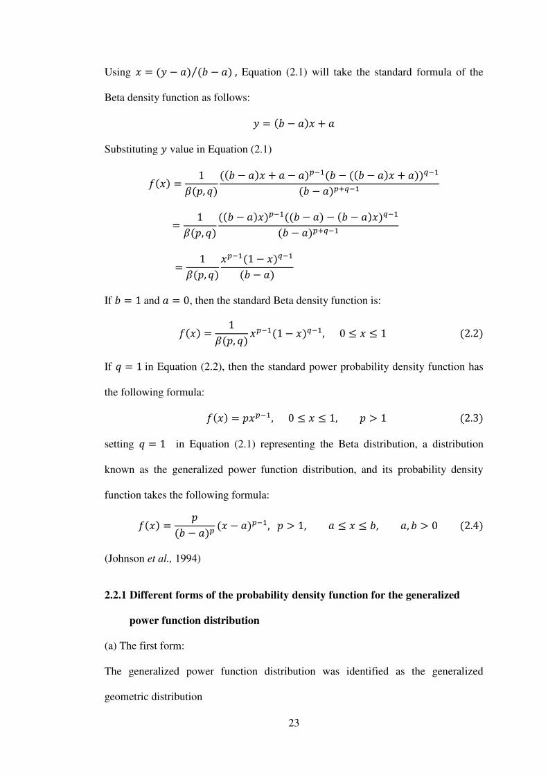
Using = − − ,⁄ Equation (2.1) will take the standard formula of the

Beta density function as follows: = − +

Substituting value in Equation (2.1)

= , − + − − − − + −− + −

= , − − − − − −− + − = , − − −−

If = and = , then the standard Beta density function is:

= , − − − , .

If = in Equation (2.2), then the standard power probability density function has

the following formula: = − , , > .

setting = in Equation (2.1) representing the Beta distribution, a distribution

known as the generalized power function distribution, and its probability density

function takes the following formula: = − − − , > , , , > .

(Johnson et al., 1994)

2.2.1 Different forms of the probability density function for the generalized . . . .

. power function distribution

(a) The first form:

The generalized power function distribution was identified as the generalized

geometric distribution

24

= � ( − �� + ) − , , � − � � + − � .

where and are defined as:

= + √ + , = √ + , . (Sultan et al., 2002)

By setting � = , � = in Equation (2.5), the probability density function for the

standard generalized power function distribution is obtained. This form was

discussed in Sultan et al. (2002). = + − , − − , > , , .

Figure 2.1 illustrates the probability density function for the standard generalized

power function with a known scale parameter = for several values of the shape

parameter and location parameter of standard generalized power function.

Figure 2.1. Probability density functions for the standard generalized power . . . . . .

. function distribution with a known scale parameter = .

(b) The second form:

The second form is seen in Equation (2.4), which expresses the generalized power

function distribution. It can be proven that this Equation is equivalent to Equation

00.10.20.30.40.50.60.70.80.9

11.1

0 0.1 0.2 0.3 0.4 0.5 0.6

f(y)

y

a=0.1,p=0.1

a=0.5,p=0.2

a=0.3,p=0.9