Journal of Engineering Science and Technology Vol. 10, No. 8 (2015) 1035 - 1053 © School of Engineering, Taylor’s University 1035 A MODIFIED DECOMPOSITION METHOD FOR SOLVING NONLINEAR PROBLEM OF FLOW IN CONVERGING- DIVERGING CHANNEL MOHAMED KEZZAR 1 , MOHAMED RAFIK SARI 1, 2, *, RACHID ADJABI 2 , AMMAR HAIAHEM 2 1 Mechanical Engineering Department, University of Skikda, El Hadaiek Road, B.O. 26, 21000 Skikda, Algeria 2 Laboratory of Industrial Mechanics, University Badji Mokhtar of Annaba, B. O. 12, 23000 Annaba, Algeria *Corresponding Author: [email protected] Abstract In this research, an efficient technique of computation considered as a modified decomposition method was proposed and then successfully applied for solving the nonlinear problem of the two dimensional flow of an incompressible viscous fluid between nonparallel plane walls. In fact this method gives the nonlinear term Nu and the solution of the studied problem as a power series. The proposed iterative procedure gives on the one hand a computationally efficient formulation with an acceleration of convergence rate and on the other hand finds the solution without any discretization, linearization or restrictive assumptions. The comparison of our results with those of numerical treatment and other earlier works shows clearly the higher accuracy and efficiency of the used Modified Decomposition Method. Keywords: Inclined walls, Jeffery-Hamel flow, Nonlinear problem, Velocity profiles, Skin friction, Modified Decomposition Method (MDM). 1. Introduction The radial two dimensional flow of an incompressible viscous fluid between two inclined plane walls separated by an angle 2α driven by a line source or sink known as Jeffery-Hamel flow, is one of the few exact solutions of the Navier-Stokes equations. The nonlinear governing equation of this flow has been discovered by Jeffery [1] and independently by Hamel [2]. Since then, several contributions have been conducted in order to solve the nonlinear problem of Jeffery-Hamel flow. Indeed, Rosenhead [3] gives on the one hand the solution in terms of elliptic function

Welcome message from author
This document is posted to help you gain knowledge. Please leave a comment to let me know what you think about it! Share it to your friends and learn new things together.
Transcript

Journal of Engineering Science and Technology Vol. 10, No. 8 (2015) 1035 - 1053 © School of Engineering, Taylor’s University
1035
A MODIFIED DECOMPOSITION METHOD FOR SOLVING NONLINEAR PROBLEM OF FLOW IN CONVERGING-
DIVERGING CHANNEL
MOHAMED KEZZAR1, MOHAMED RAFIK SARI
1, 2,*,
RACHID ADJABI2, AMMAR HAIAHEM
2
1Mechanical Engineering Department, University of Skikda, El Hadaiek Road, B.O. 26,
21000 Skikda, Algeria 2Laboratory of Industrial Mechanics, University Badji Mokhtar of Annaba, B. O. 12,
23000 Annaba, Algeria
*Corresponding Author: [email protected]
Abstract
In this research, an efficient technique of computation considered as a modified decomposition method was proposed and then successfully applied for solving
the nonlinear problem of the two dimensional flow of an incompressible
viscous fluid between nonparallel plane walls. In fact this method gives the
nonlinear term Nu and the solution of the studied problem as a power series.
The proposed iterative procedure gives on the one hand a computationally
efficient formulation with an acceleration of convergence rate and on the other hand finds the solution without any discretization, linearization or restrictive
assumptions. The comparison of our results with those of numerical treatment
and other earlier works shows clearly the higher accuracy and efficiency of the
used Modified Decomposition Method.
Keywords: Inclined walls, Jeffery-Hamel flow, Nonlinear problem, Velocity profiles, Skin friction, Modified Decomposition Method (MDM).
1. Introduction
The radial two dimensional flow of an incompressible viscous fluid between two
inclined plane walls separated by an angle 2α driven by a line source or sink known
as Jeffery-Hamel flow, is one of the few exact solutions of the Navier-Stokes
equations. The nonlinear governing equation of this flow has been discovered by
Jeffery [1] and independently by Hamel [2]. Since then, several contributions have
been conducted in order to solve the nonlinear problem of Jeffery-Hamel flow.
Indeed, Rosenhead [3] gives on the one hand the solution in terms of elliptic function

1036 M. Kezzar et al.
Journal of Engineering Science and Technology August 2015, Vol. 10(8)
Nomenclatures
An Adomian polynomials
a Constant of divergent channel
b Constant of divergent channel
c Constant of convergent channel
cf Skin friction coefficient
d Derivative operator
F Non-dimensional velocity or general nonlinear operator
F′ First derivative of velocity
F′′ Second derivative of velocity
f Velocity
fmax Velocity at the centerline of channel
g Function
Lu Linear operator
L-1
Inverse or integral operator
n Number of iteration
Nu Nonlinear operator
P Fluid pressure, N/m2
r Radial coordinate, m
Re Reynolds number
Rec Critical Reynolds number
Ru Remainder of linear operator
u Function or velocity
Vmax Maximal velocity, m/s
Vr Radial velocity, m/s
Vz Axial velocity, m/s
Vθ Azimuthal velocity, m/s
x Cartesian coordinate, m
z Axial coordinate, m
Greek Symbols
η Non-dimensional angle
θ Angular coordinate, deg.
α Channel half-angle, deg.
αc Critical channel half-angle, deg. ϕ Constant ρ Density, kg/m3
ν Kinematic viscosity, m2/s
∂ Derivative operator
∞ Condition at infinity
Abbreviations
ADM Adomian decomposition method
HPM Homotopy perturbation method
MDM Modified decomposition method
and discuss on the other hand the various mathematically possible types of this
flow. The exact solution of thermal distributions of the Jeffery-Hamel flow has
been given by Millsaps and pohlhausen [4]. In this contribution, temperature

A Modified Decomposition Method for Solving Nonlinear Problem of . . . . 1037
Journal of Engineering Science and Technology August 2015, Vol. 10(8)
distributions due only to dissipation have been calculated numerically in
converging-diverging channels. Fraenkel [5] investigated the laminar flow in
symmetrical channels with slightly curved walls. In this study the resulting
velocity profiles of the flow were obtained as a power series. The nonlinear
problem of the Jeffery-Hamel flow in converging-diverging channels has been
also well discussed in many textbooks [6-8].
The two dimensional stability of Jeffery-Hamel flow has been extensively
studied by many authors. Uribe et al. [9] used the Galerkin method to study linear
and temporal stability of some flows for small widths of the channel. Sobey et al.
[10] in their study suggested that the radial flows (convergent or divergent) are
unstable. Banks et al. [11] treated the temporal and spatial stability of Jeffery-
Hamel flow. Critical values of Reynolds numbers for Jeffery-Hamel flow have
been computed by Hamadiche et al. [12]. Makinde et al. [13] also studied the
temporal stability of the Jeffery-Hamel flow in convergent-divergent channels
under the effect of an external magnetic field. The principal eigenvalues for some
family of Jeffery-Hamel flows in diverging channels have been calculated by
CARMI [14]. The linear temporal three dimensional stability of incompressible
viscous flow in a rotating divergent channel is studied by Al Farkh et al. [15].
Eagles [16] for his part, investigated the linear stability of Jeffery-Hamel flows by
solving numerically the relevant Orr-Sommerfeld problem.
In recent years several methods were developed in order to solve analytically the
nonlinear initial or boundary value problem, such as the homotopy method [17-20],
the variational iteration method [21-23] and the Adomian decomposition method
[24-26]. These methods have been successfully applied for solving mathematical
and physical problems. Indeed, many authors [27-31] have used these new
approximate analytical methods to study the nonlinear problem of Jeffery-Hamel
flow. Motsa et al. for their part [32] undertook a study on the nonlinear problem of
magnetohydrodynamic Jeffery-Hamel flow by using a novel hybrid spectral
homotopy analysis technique. The Adomian decomposition method has been also
successfully used [33, 34] in the solution of Blasius equation and the two
dimensional laminar boundary layer of Falkner-Skan for wedge.
In the present research, the solution of two dimensional flow of an
incompressible viscous fluid between nonparallel plane walls is presented. The
resulting third order differential equation is solved analytically by a modified
decomposition method and the obtained results are compared to the numerical
results. The principal aim of this study is on the one hand to find approximate
analytical solutions of Jeffery-Hamel flow in convergent-divergent channels and
on the other hand to investigate the accuracy and efficiency of the adopted
Modified Decomposition Method.
2. Governing Equations
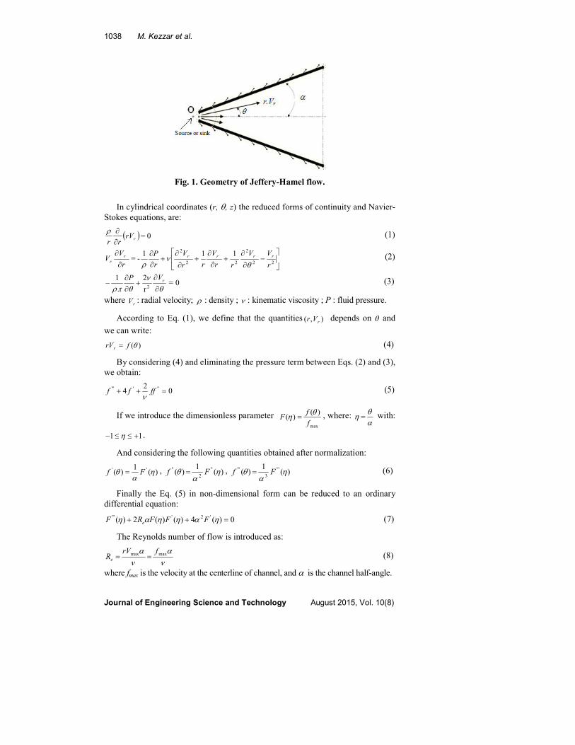
In this research the flow of an incompressible viscous fluid between nonparallel
plane walls has been studied. The geometrical configuration of the Jeffery-Hamel
flow is given in Fig. 1. Indeed, the considered flow is uniform along the z-
direction and we assume purely radial motion, i.e.: for velocity components we
can write: )0);,(( === zr VVrVV θθ
1038 M. Kezzar et al.
Journal of Engineering Science and Technology August 2015, Vol. 10(8)
Fig. 1. Geometry of Jeffery-Hamel flow.
In cylindrical coordinates (r, θ, z) the reduced forms of continuity and Navier-
Stokes equations, are:
( ) 0=rrVrr ∂
∂ρ (1)
−
∂
∂+
∂
∂+
∂
∂+
∂∂
∂
∂22
2
22
2111
-=r
VV
rr
V
rr
V
r
P
r
VV rrrrr
r θν
ρ (2)
0=r
2
.r
12 θν
θρ ∂
∂+
∂∂
− rVP (3)
where rV : radial velocity; ρ : density ; ν : kinematic viscosity ; P : fluid pressure.
According to Eq. (1), we define that the quantities ),( rVr depends on θ and
we can write:
)(θfrVr = (4)
By considering (4) and eliminating the pressure term between Eqs. (2) and (3),
we obtain:
02
4 '''''' =++ ffffν
(5)
If we introduce the dimensionless parameter max
)()(
f
fF
θη = , where:
αθ
η = with:
11 +≤≤− η .
And considering the following quantities obtained after normalization:
)(1
)( '' ηα
θ Ff = , )(1
)( ''
2
'' ηα
θ Ff = , )(1
)( '''
3
''' ηα
θ Ff = (6)
Finally the Eq. (5) in non-dimensional form can be reduced to an ordinary
differential equation:
0)(4)()(2)('2'''' =++ ηαηηαη FFFRF e
(7)
The Reynolds number of flow is introduced as:
να
να maxmax frV
Re == (8)
where fmax is the velocity at the centerline of channel, and α is the channel half-angle.

A Modified Decomposition Method for Solving Nonlinear Problem of . . . . 1039
Journal of Engineering Science and Technology August 2015, Vol. 10(8)
The boundary conditions of the Jeffery-Hamel flow in terms of )(ηF are
expressed as follows:
at the centerline of channel 0)(,1)( ' == ηη FF (9)
at the body of channel 0)( =±ηF (10)
3. Modified Decomposition Method Formulation
Consider the differential equation:
)(tgNuRuLu =++ (11)
where: N is a nonlinear operator, L is the highest ordered derivative and R
represents the remainder of linear operator L.
By considering1−L as an n-fold integration for an nth order of L, the principles
of method consists on applying the operator 1−L to the expression (11). Indeed,
we obtain:
NuLRuLgLLuL 1111 −−−− −−= (12)
The solution of Eq. (12) is given by:
NuLRuLgLu 111 −−− −−+= ϕ (13)
where ϕ is determined from the boundary or initial conditions.
Normally for the standard Adomian decomposition method, the solution u can
be determined as an infinite series with the components given by:
nn uu ∞=∑= 0
(14)
And the nonlinear term Nu is given as following:
),.......,,( 100 nnn uuuANu ∞=∑= (15)
where sAn ' is called Adomian polynomials and has been introduced by George
Adomian [24] by the recursive formula:
( )[ ] nnuNd
d
nuuuA i
i
in
n
nn ,.......,2,1,0,1
),.......,,(
0
010 =
∑
Ι=
=
∞=
• λ
λλ
(16)
By substituting the given series (14), (15) into both sides of (13), we obtain
the following expressions:
nnnnnn ALuRLgLu ∞=
−∞=
−−∞= ∑−∑−+=∑ 0
1
0
11
0 ϕ (17)
According to Eq. (17), the recursive expression which defines the ADM
components nu is given as:
)(, 1
1
1
0 nnn ARuLugLu +−=+= −+
−ϕ (18)
For the adopted modified decomposition method, based on the idea of power
series method, we assume that the solution � and the nonlinear term Nu can be
decomposed respectively as:
n
nn xuu ∞=∑= 0
(19) n
nnn xuuuAu ),.......,,( 100
∞=∑= (20)

1040 M. Kezzar et al.
Journal of Engineering Science and Technology August 2015, Vol. 10(8)
When Adomian polynomials nA are known, the components of the solution u,
for the adopted Modified Decomposition Method are expressed as follows:
n
nnn xARuLugLu )(, 1
1
1
0 +−=+= −+
−ϕ (21)
Finally after some iteration, the solution of the studied equation can be given
as a power series as follows:
n
n xuxuxuxuuu ++++++= ........3
3
2
210 (22)
4. Application of MDM to the Jeffery-Hamel Problem
Considering the Eq. (11), Eq. (7) can be written as:
'2' 42 FFFRLF e αα −−= (23)
where the differential operator L is given by: 3
3
dn
dL = .
The inverse of operator L is expressed by 1−L and can be represented as:
∫ ∫ ∫ •=−η η η
ηηη0 0 0
1 )( dddL (24)
The application of Eq. (24) on Eq. (23) and considering the boundary
conditions (9) and (10), we obtain:
)(2
)0()0()0()(1
2'''
NuLFFFF−+++=
ηηη (25)
where: '2' 42 FFFRNu e αα −−= (26)
The values of )0(),0( 'FF and )0(''F depend on boundary conditions for
convergent-divergent channels. In order to distinguish between convergent and
divergent channels, the boundary conditions are taken with different manner [29].
Indeed, on the one hand for divergent channel, we assume that the body of
channel is given by 0=η and by considering a symmetric condition in the center
of channel; the solution is studied between 0)0( =F at the body of channel and
1)1( =F at the centerline of channel. On the other hand, for convergent channels,
the center of channel is given by 0=η and consequently the solution varies from
0)1( =F at the body of channel to 1)0( =F at the centerline of channel.
4.1. Convergent channel:
For convergent channel the boundary conditions are expressed as follows:
at the centerline of channel 0)0(,1)0( ' == FF (27)
at the body of channel 0)1( =F (28)

A Modified Decomposition Method for Solving Nonlinear Problem of . . . . 1041
Journal of Engineering Science and Technology August 2015, Vol. 10(8)
In this case, the solution of our problems is studied between 0)1( =F at the
body of channel and 1)0( =F at the centerline of channel. By applying the
boundary conditions (27), (28) and considering cF =)0('' , we obtain:
)()( 1
00 NuLFFF nn
−∞= +=∑=η (29)
where:
21
2
0
ηcF += (30)
According to the modified decomposition method, Adomian polynomials and
solutions terms will be computed as follows:
322
0 42 αηηααη ee RcccRA −−−= (31)
62424
1120
1
6
1
12
1αηηααη ee RcccRF −−−= (32)
82246336223
4424324222
1
40
1
15
8
15
4
3
2
3
2
6
1
ηαηαηα
ηαηαηα
eee
ee
RcRcRc
cRcRcA
+++
+++= (33)
12224103310223
8428328222
2
52800
1
1350
1
2700
1
504
1
504
1
2016
1
ηαηαηα
ηαηαηα
eee
ee
RcRcRc
cRcRcF
+++
+++= (34)
1433613336
124251233511425
11335105410424
1033495494249334
86385384238333
2
17600
1
4800
1
39600
91
79200
91
120
1
240
1
37800
337
37800
337
151200
337
12
1
12
1
48
1
126
1
84
1
168
1
1008
1
ηαηα
ηαηαηα
ηαηαηα
ηαηαηαηα
ηαηαηαηα
ee
eee
eee
eeee
eee
RcRc
RcRcRc
RcRcRc
RcRcRcRc
cRcRcRcA
−−
−−−
−−−
−−−−
−−−−=
(35)
1933618336
1742517335
16425163351554
15424153341454
14424143341363
13531342313333
3
102326400
1
23500800
1
161568000
91
323136000
91
403200
1
806400
1
103194000
337
103194000
337
412776000
337
26208
1
26208
1
104832
1
216216
1
144144
1
288288
1
1729728
1
ηαηα
ηαηα
ηαηαηα
ηαηαηα
ηαηαηα
ηαηαηα
ee
ee
eee
eee
ee
eee
RcRc
RcRc
RcRcRc
RcRcRc
RcRcc
RcRcRcF
−−
−−
−−−
−−−
−−−
−−−=
(36)
1042 M. Kezzar et al.
Journal of Engineering Science and Technology August 2015, Vol. 10(8)
Finally, the solution for convergent channel is given by the modified
decomposition method as a power series as following:
n
nFFFFFF ηηηηη +++++= ........)( 3
3
2
210 (37)
The value of constant c is obtained by solving Eq. (37) using Eq. (28).
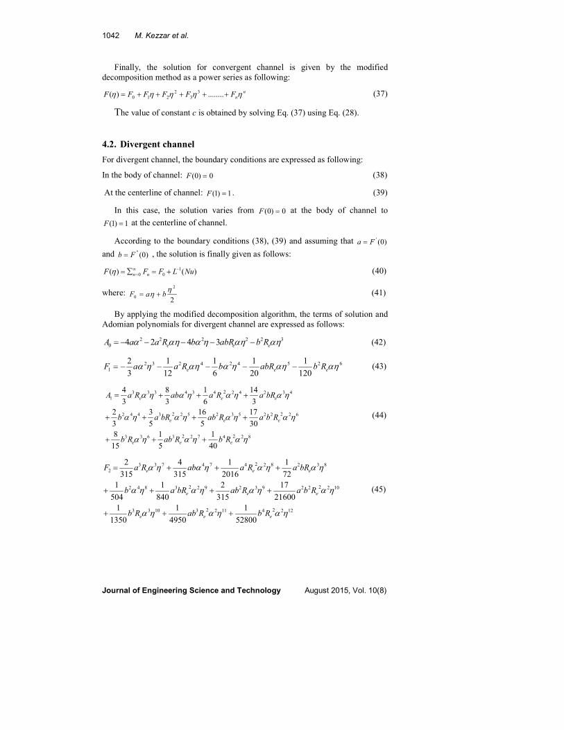
4.2. Divergent channel
For divergent channel, the boundary conditions are expressed as following:
In the body of channel: 0)0( =F (38)
At the centerline of channel: 1)1( =F . (39)
In this case, the solution varies from 0)0( =F at the body of channel to
1)1( =F at the centerline of channel.
According to the boundary conditions (38), (39) and assuming that )0('Fa =
and )0(''Fb = , the solution is finally given as follows:
)()( 1
00 NuLFFF nn
−∞= +=∑=η (40)
where: 2
2
0
ηη baF += (41)
By applying the modified decomposition algorithm, the terms of solution and
Adomian polynomials for divergent channel are expressed as follows:
322222
0 3424 αηαηηααηα eee RbabRbRaaA −−−−−= (42)
625424232
1120
1
20
1
6
1
12
1
3
2αηαηηααηηα eee RbabRbRaaF −−−−−= (43)
82247223633
622225325223442
432422434333
1
40
1
5
1
15
8
30
17
5
16
5
3
3
2
3
14
6
1
3
8
3
4
ηαηαηα
ηαηαηαηα
ηαηαηαηα
eee
eee
eee
RbRabRb
RbaRabbRab
bRaRaabRaA
+++
++++
+++=
(44)
12224112231033
1022229329223842
832822474733
2
52800
1
4950
1
1350
1
21600
17
315
2
840
1
504
1
72
1
2016
1
315
4
315
2
ηαηαηα
ηαηαηαηα
ηαηαηαηα
eee
eee
eee
RbRabRb
RbaRabbRab
bRaRaabRaF
+++
++++
+++=
(45)
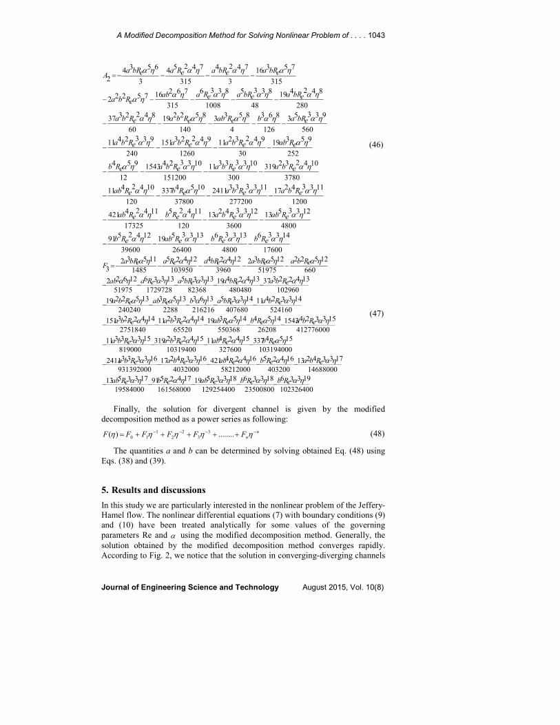
A Modified Decomposition Method for Solving Nonlinear Problem of . . . . 1043
Journal of Engineering Science and Technology August 2015, Vol. 10(8)
17600
14336
4800
13336
26400
1333519
39600
1242591
4800
1233513
3600
12334213
120
11425
17325
11424421
1200
11334217
277200
1133332411
37800
1054337
120
1042411
3780
104232319
300
10333311
151200
1033241543
12
954
252
95319
30
9423211
1260
94223151
240
9332411
560
93353
126
863
4
8533
140
852219
60
8422337
280
842419
48
8335
1008
8336
315
7621675222
315
75316
3
7424
315
74254
3
65342
ηαηαηαηα
ηαηαηαηα
ηαηαηαηα
ηαηαηαηα
ηαηαηαηα
ηαηαηαηαηα
ηαηαηαηαηα
ηαηαηαηα
eRbeRbeRabeRb
eRabeRbaeRbeRab
eRbaeRbaeRbeRab
eRbaeRbaeRbaeRb
eRabeRbaeRbaeRba
ebRabeRabeRbaeRba
ebRaebRaeRaabeRba
ebRaebRaeRaebRaA
−−−−
−−−−
−−−−
−−−−
−−−−
−−−−−
−−−−−
−−−−=
(46)
102326400
19336
23500800
18336
129254400
1833519
161568000
1742591
19584000
1733513
14688000
17334213
403200
16425
58212000
16424421
4032000
16334217
931392000
1633332411
103194000
1554337
327600
1542411
10319400
154232319
819000
15333311
412776000
1533241543
26208
1454
550368
145319
65520
14423211
2751840
144223151
524160
14332411
407680
14335
216216
1363
2288
1353
240240
1352219
102960
13422337
480480
1342419
82368
13335
1729728
13336
51975
12622
660
12522
51975
12532
3960
12424
103950
12425
1485
115323
ηαηαηαηαηα
ηαηαηαηαηα
ηαηαηαηα
ηαηαηαηαηα
ηαηαηαηαηα
ηαηαηαηαηα
ηαηαηαηαηα
eRbeRbeRabeRbeRab
eRbaeRbeRabeRbaeRba
eRbeRabeRbaeRba
eRbaeRbeRabeRbaeRba
eRbaebRabeRabeRba
eRbaebRaebRaeRaab
eRbaebRaebRaeRaebRaF
−−−−−
−−−−−
−−−−
−−−−−
−−−−−
−−−−−
−−−−−=
(47)
Finally, the solution for divergent channel is given by the modified
decomposition method as a power series as following:
n
nFFFFFF −−−− +++++= ηηηηη ........)( 3
3
2
2
1
10 (48)
The quantities a and b can be determined by solving obtained Eq. (48) using
Eqs. (38) and (39).
5. Results and discussions
In this study we are particularly interested in the nonlinear problem of the Jeffery-
Hamel flow. The nonlinear differential equations (7) with boundary conditions (9)
and (10) have been treated analytically for some values of the governing
parameters Re and α using the modified decomposition method. Generally, the
solution obtained by the modified decomposition method converges rapidly.
According to Fig. 2, we notice that the solution in converging-diverging channels

1044 M. Kezzar et al.
Journal of Engineering Science and Technology August 2015, Vol. 10(8)
for small Reynolds number (Re= 100) converges quickly to the numerical
solution. Indeed, analytical solution converges at the first iteration in convergent
flow and in the third iteration for divergent flow. As it is clear in Fig. 3 when
Reynolds number becomes higher (Re= 216), the obtained solution by modified
decomposition method converges after 3 iterations for convergent channel and
after 5 iterations for divergent channel.
a) Convergent Channel b) Divergent Channel
Fig. 2. Velocity profiles by MDM after iteration for Re=100, αααα=5°°°°.
a) Convergent Channel b) Divergent Channel
Fig. 3. Velocity profiles by MDM after iteration for Re=216, αααα=5°°°°.
In order to test the accuracy, applicability and efficiency of this new Modified
Decomposition Method, a comparison with the numerical results obtained by
fourth order Runge Kutta method is performed. We notice that the comparison
shows an excellent agreement between analytical and numerical data for
convergent and divergent channels, as presented in Tables 1 and 2. In these tables,
the error is introduced as:
')()( NumMDM FFError ηη −=
A Modified Decomposition Method for Solving Nonlinear Problem of . . . . 1045
Journal of Engineering Science and Technology August 2015, Vol. 10(8)
As it is shown in Tables 3 and 4 in comparison with the standard Adomian
method and the Homotopy perturbation method for diverging channel, we notice
that the MDM technique has a high precision than ADM and HPM. Clearly,
results show that the MDM solution converges quickly after five iteration of
computation. It is also noted that both analytical and numerical results are in
excellent agreement.
Ta
ble
1.
Co
mp
aris
on
betw
een
th
e N
um
eri
cal
an
d M
DM
res
ult
s
for v
elo
cit
y d
istr
ibu
tio
n i
n c
on
verg
ing c
ha
nn
el
wh
en:
αα αα=
3°° °°.
Ta
ble
2 t
he c
om
paris
on
bet
ween
th
e N
um
eric
al
an
d M
DM
resu
lts
for v
elo
cit
y i
n d
iver
gin
g c
ha
nn
el
wh
en
: αα αα
=3°° °°.
ηη ηη
Re=
10
0
Re=
150
Re=
300
R
e=4
00
Nu
mer
ical
MD
M
Error
Nu
meri
cal
MD
M
Err
or
Nu
meri
cal
MD
M
Erro
r
Nu
mer
ica
l M
DM
E
rro
r
0
1.0
000
0
1.0
0000
0.0
00000
1.0
0000
0
1.0
000
00
0.0
0000
0
1.0
0000
0
1.0
00000
0.0
000
00
1.0
000
00
1.0
0000
0
0.0
00000
0.2
0
.979311
0.9
7931
1
0.0
00000
0.9
8496
8
0.9
849
68
0.0
0000
0
0.9
9384
1
0.9
93840
0.0
000
01
0.9
964
15
0.9
9641
3
0.0
00002
0.4
0
.908482
0.9
0848
2
0.0
00000
0.9
3010
0
0.9
301
00
0.0
0000
0
0.9
6685
0
0.9
66846
0.0
000
04
0.9
788
03
0.9
7879
0
0.0
00013
0.6
0
.759108
0.7
5910
8
0.0
00000
0.8
0124
9
0.8
012
49
0.0
0000
0
0.8
8261
3
0.8
82600
0.0
000
13
0.9
140
56
0.9
1400
3
0.0
00053
0.8
0
.479108
0.4
7926
9
0.0
00161
0.5
2753
8
0.5
275
38
0.0
0000
0
0.6
3677
1
0.6
36739
0.0
000
32
0.6
886
27
0.6
8847
5
0.0
00152
1
0.0
00000
0.0
0000
0
0.0
00000
0.0
0000
0
0.0
000
00
0.0
0000
0
0.0
0000
0
0.0
00000
0.0
000
00
0.0
000
00
0.0
0000
0
0.0
00000
ηη ηη
Re=
10
0
Re=
15
0
Re=
30
0
Re=
40
0
Nu
mer
ica
l M
DM
E
rro
r
Nu
meri
ca
l M
DM
E
rro
r
Nu
meri
ca
l M
DM
E
rro
r N
um
eric
al
MD
M
Err
or
0
0.0
00
00
0
0.0
00
00
0
0.0
000
00
0
.00
00
00
0
.00
00
00
0
.00
00
00
0.0
00
00
0
0.0
00
00
0
0.0
000
00
0
.00
00
00
0.0
000
00
0.0
00
00
0
0.2
0
.21
30
26
0.2
13
01
9
0.0
000
07
0
.13
66
11
0
.13
65
87
0
.00
00
24
-0.0
57
25
3
-0.0
57
280
0
.00
00
27
-0
.14
50
84
-0.1
45
119
0
.00
00
35
0.4
0
.46
66
47
0.4
66
63
5
0.0
000
12
0
.36
59
96
0
.36
59
54
0
.00
00
40
0.0
81
61
2
0.0
81
55
8
0.0
000
54
-0
.05
95
31
-0.0
59
607
0
.00
00
76
0.6
0
.72
44
35
0.7
24
42
4
0.0
000
11
0
.64
96
19
0
.64
95
75
0
.00
00
56
0.4
06
02
2
0.4
05
95
0
0.0
000
72
0
.26
29
16
0.2
627
99
0.0
00
11
7
0.8
0
.92
39
55
0.9
23
94
9
0.0
000
06
0
.89
86
68
0
.89
86
42
0
.00
00
26
0.8
05
20
9
0.8
05
15
7
0.0
000
52
0
.74
02
70
0.7
401
69
0.0
00
10
1
1
1.0
00
00
0
1.0
000
0
0.0
000
00
1
.00
00
00
1
.00
00
00
0
.00
00
00
1.0
00
00
0
1.0
00
00
0
0.0
000
00
1
.00
00
00
1.0
000
00
0.0
00
00
0
1046 M. Kezzar et al.
Journal of Engineering Science and Technology August 2015, Vol. 10(8)
Table 3 Comparison of the MDM results
against the numerical and ADM for F(ηηηη) when αααα=5°°°°, Re=50.
HPM
[30] Numerical
MDM
(Present study)
ADM
(Present study)
F(η) F(η) F(η) F(η) F(η) F(η) F(η)
η
3rd
order
5th
order
3rd
order
5th
order
9th
order
0 1 1 1 1 1 1 1
0.25 0.894960 0.894242 0.894342 0.894238 0.880756 0.891679 0.891602
0.50 0.627220 0.626948 0.627103 0.626942 0.604680 0.621332 0.619762
0.75 0.302001 0.301990 0.302102 0.301986 0.285037 0.296600 0.294271
1 0 0 0 0 0 0 0
Table 4 Comparison of the MDM results
against the numerical and ADM for F′′′′′′′′(ηηηη) when αααα=5°°°°, Re=50.
HPM [30] Numerical MDM (Present study) ADM (Present study)
η F''(η) F''(η) F''(η) F''(η) F''(η) F''(η) F''(η)
3rd order 5th order 3rd order 5th order 9th order
0 -3.539214 -3.539416 -3.530365 -3.539803 -4.637850 -3.712261 -3.63750
0.25 -2.661930 -2.662084 -2.663422 -2.662031 -2.513760 -2.665958 -2.69556
0.50 -0.879711 -0.879794 -0.881423 -0.879736 -0.643805 -0.824410 -0.812129
0.75 0.447331 0.447244 0.446170 0.447281 0.630888 0.530321 0.580548
1 0.854544 0.854369 0.853594 0.854395 1.011719 0.959673 1.0395
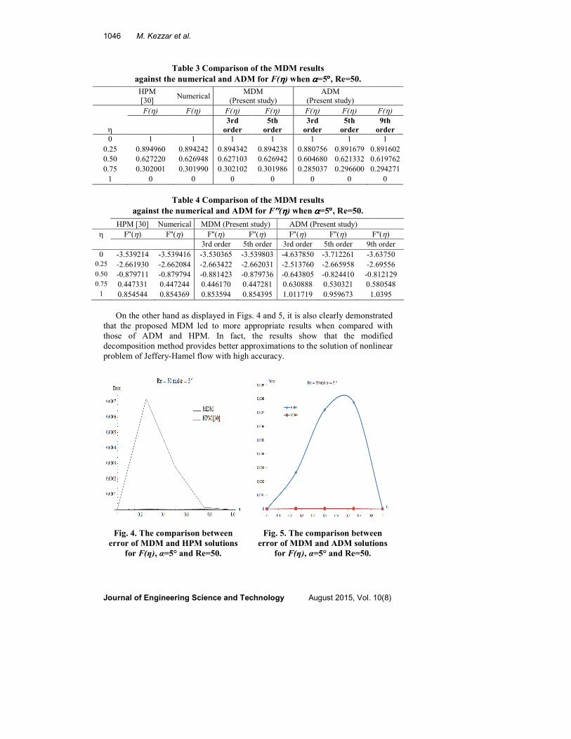
On the other hand as displayed in Figs. 4 and 5, it is also clearly demonstrated
that the proposed MDM led to more appropriate results when compared with
those of ADM and HPM. In fact, the results show that the modified
decomposition method provides better approximations to the solution of nonlinear
problem of Jeffery-Hamel flow with high accuracy.
Fig. 4. The comparison between
error of MDM and HPM solutions
for F(η), α=5° and Re=50.
Fig. 5. The comparison between
error of MDM and ADM solutions
for F(η), α=5° and Re=50.

A Modified Decomposition Method for Solving Nonlinear Problem of . . . . 1047
Journal of Engineering Science and Technology August 2015, Vol. 10(8)
With intention to show the importance of the studied flow, the numerical and
analytical values are plotted in Figs. 6-15. Indeed, these figures show the velocity
profiles in convergent-divergent channels.
Figure 6 shows the velocity profiles in channel of half angle, α = 7° and fixed
Reynolds number (Re= 126) for purely convergent flow. As it clear, the
dimensionless velocity decreased from 1 at 0=η to values 0 at 1±=η . The
effect of Reynolds number on velocity profiles for convergent flow is depicted in
Fig. 7. Indeed, increasing Reynolds number leads on the one hand to a flatter
profile at the centre of channel with high gradients near the walls and on the other
hand to decreased thickness of the boundary layer. We notice also that the
velocity profiles are symmetric against 0=η and the symmetric convergent flow
is possible for opening angle 2α not exceed π . It is also clear for convergent
channels that the backflow is excluded.
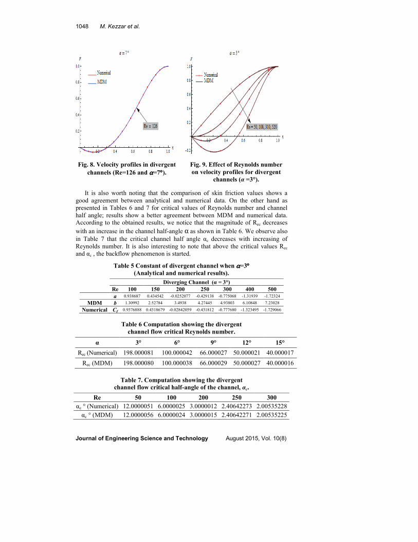
The variation of velocity profiles in divergent channels for a fixed Reynolds
number (Re= 126) when α = 7° is investigated in Fig. 8. Obtained results show
that the velocity increased from 0 at 0=η to 1 at 1±=η . The effect of
Reynolds number on divergent flow (Fig. 9) is to concentrate the volume flux at
the centre of channels with smaller gradients near the walls and consequently
the thickness of boundary layer increase. For purely divergent channels,
symmetric flow is not possible for an opening angle 2α , unless for Reynolds
numbers not exceed a critical value. Above this critical Reynolds number, we
observe clearly that the separation and backflow are started (see Fig. 10 and
Table 5). In fact, the negative values of skin friction indicate on the beginning
of the backflow phenomenon.
In Table 5 are listed the values of )0(),0( ''' FF and cf. Indeed, )0('F and )0(''F
are investigated analytically by the modified decomposition method, but fc is
evaluated numerically by fourth order Runge Kutta method.
Fig. 6. Velocity profiles in convergent
channels (Re=126 and αααα=7°°°°).
Fig. 7. Effect of Reynolds number on
velocity profiles for convergent
channels (αααα=3°°°°).
1048 M. Kezzar et al.
Journal of Engineering Science and Technology August 2015, Vol. 10(8)
Fig. 8. Velocity profiles in divergent
channels (Re=126 and αααα=7°°°°).
Fig. 9. Effect of Reynolds number
on velocity profiles for divergent
channels (α =3°).
It is also worth noting that the comparison of skin friction values shows a
good agreement between analytical and numerical data. On the other hand as
presented in Tables 6 and 7 for critical values of Reynolds number and channel
half angle; results show a better agreement between MDM and numerical data.
According to the obtained results, we notice that the magnitude of Rec decreases
with an increase in the channel half-angle α as shown in Table 6. We observe also
in Table 7 that the critical channel half angle αc decreases with increasing of
Reynolds number. It is also interesting to note that above the critical values Rec
and αc , the backflow phenomenon is started.
Table 5 Constant of divergent channel when αααα=3°°°°
(Analytical and numerical results).
Table 6 Computation showing the divergent
channel flow critical Reynolds number.
α 3° 6° 9° 12° 15°
Rec (Numerical) 198.000081 100.000042 66.000027 50.000021 40.000017
Rec (MDM) 198.000080 100.000038 66.000029 50.000027 40.000016
Table 7. Computation showing the divergent
channel flow critical half-angle of the channel, αc.
Re 50 100 200 250 300
αc ° (Numerical) 12.0000051 6.0000025 3.0000012 2.40642273 2.00535228
αc ° (MDM) 12.0000056 6.0000024 3.0000015 2.40642271 2.00535225
Diverging Channel (α = 3°)
Re 100 150 200 250 300 400 500
a 0.938687 0.434542 -0.0252077 -0.429138 -0.775068 -1.31939 -1.72324
MDM b 1.30992 2.52784 3.4938 4.27445 4.93803 6.10848 7.23028
Numerical Cf 0.9376888 0.4318679 -0.02842059 -0.431812 -0.777680 -1.323495 -1.729066
A Modified Decomposition Method for Solving Nonlinear Problem of . . . . 1049
Journal of Engineering Science and Technology August 2015, Vol. 10(8)
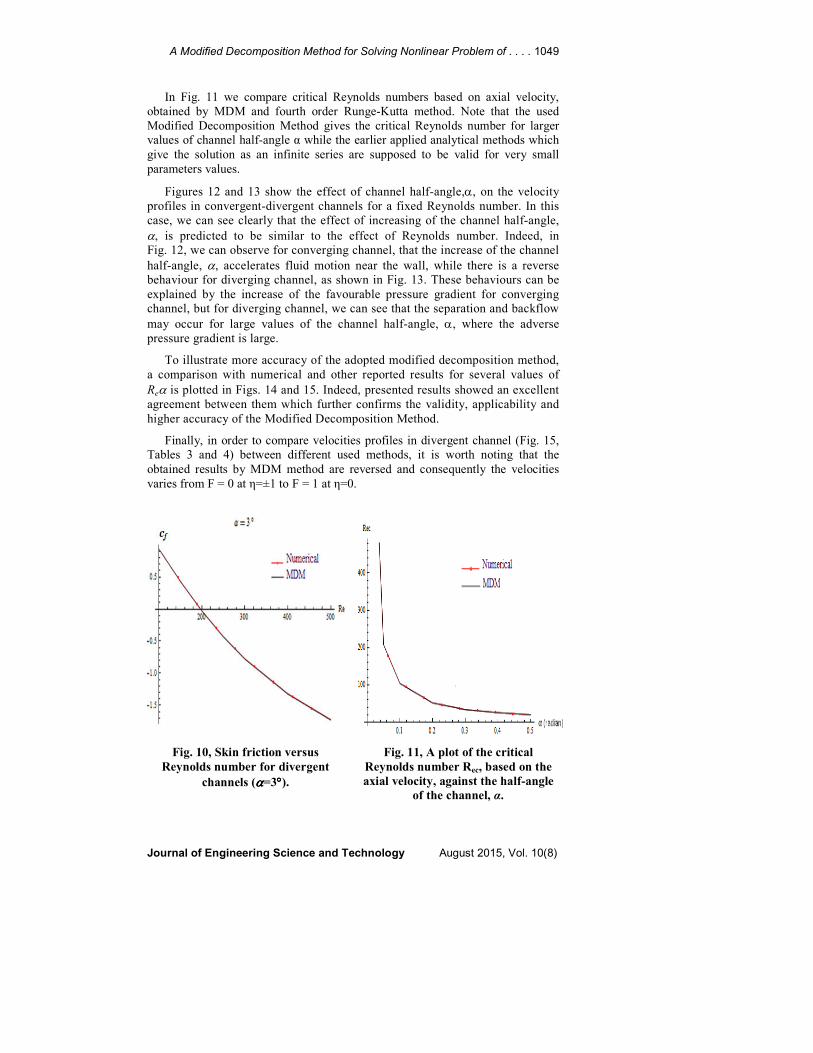
In Fig. 11 we compare critical Reynolds numbers based on axial velocity,
obtained by MDM and fourth order Runge-Kutta method. Note that the used
Modified Decomposition Method gives the critical Reynolds number for larger
values of channel half-angle α while the earlier applied analytical methods which
give the solution as an infinite series are supposed to be valid for very small
parameters values.
Figures 12 and 13 show the effect of channel half-angle,α, on the velocity
profiles in convergent-divergent channels for a fixed Reynolds number. In this
case, we can see clearly that the effect of increasing of the channel half-angle,
α, is predicted to be similar to the effect of Reynolds number. Indeed, in
Fig. 12, we can observe for converging channel, that the increase of the channel
half-angle, α, accelerates fluid motion near the wall, while there is a reverse
behaviour for diverging channel, as shown in Fig. 13. These behaviours can be
explained by the increase of the favourable pressure gradient for converging
channel, but for diverging channel, we can see that the separation and backflow
may occur for large values of the channel half-angle, α, where the adverse
pressure gradient is large.
To illustrate more accuracy of the adopted modified decomposition method,
a comparison with numerical and other reported results for several values of
Reα is plotted in Figs. 14 and 15. Indeed, presented results showed an excellent
agreement between them which further confirms the validity, applicability and
higher accuracy of the Modified Decomposition Method.
Finally, in order to compare velocities profiles in divergent channel (Fig. 15,
Tables 3 and 4) between different used methods, it is worth noting that the
obtained results by MDM method are reversed and consequently the velocities
varies from F = 0 at η=±1 to F = 1 at η=0.
Fig. 10, Skin friction versus
Reynolds number for divergent
channels (αααα=3°°°°).
Fig. 11, A plot of the critical
Reynolds number Rec, based on the
axial velocity, against the half-angle
of the channel, α.

1050 M. Kezzar et al.
Journal of Engineering Science and Technology August 2015, Vol. 10(8)
Fig. 12. Effect of channel half-angle
αααα on velocity profiles for convergent
channels (Re=50).
Fig. 13. Effect of channel half-angle
αααα on velocity profiles for divergent
channels (Re=50).
Fig. 14. Comparison between
different results for convergent
channels-velocity profiles versus Reαααα.
Fig. 15. Comparison between
different results for divergent
channels-velocity profiles versus Reαααα.
6. Conclusion
In this paper the nonlinear problem of an incompressible viscous flow between
nonparallel plane walls known as Jeffery-Hamel flow is investigated analytically
and numerically. Indeed, the third order nonlinear differential equation which
governs the Jeffery-Hamel flow has been solved analytically by using a Modified
Decomposition Method and numerically via fourth order Runge Kutta method.
The principal aim of this study is to obtain an approximation of the analytical
solution of the considered problem.
The principal conclusions, which we can draw from this study, are:
• Increasing Reynolds number of convergent flow leads to a flatter profile at the
center of channels and consequently the thickness of boundary layer decrease.
A Modified Decomposition Method for Solving Nonlinear Problem of . . . . 1051
Journal of Engineering Science and Technology August 2015, Vol. 10(8)
• For divergent flow, the effect of increasing Reynolds number is to
concentrate the volume flux at the center of channels. In this case, the
thickness of boundary layer increases with increasing Reynolds number.
• The increase of the channel half-angle, α, leads to an increase of velocity in
convergent channel, while there is a reverse behaviour in velocity profiles for
divergent channel.
• For divergent channel, the separation and backflow may occur for higher
values of the channel half-angle, α, when the adverse pressure gradient is large.
• Obtained results for dimensionless velocity profiles show an excellent
agreement between MDM and numerical solution.
• In comparison with the standard Adomian method, we notice that MDM has a
high precision than ADM.
• Modified Decomposition Method gives the solution of the studied problem
for larger values of channel half angle α while the earlier applied analytical
methods which give the solution as an infinite series are supposed to be valid
only for small parameters values.
• The adopted Modified Decomposition Method gives a computationally efficient
formulation with an acceleration of convergence rate. Indeed, this method is
accurate, efficient and highly recommended to solve nonlinear physical problems
because it gives the solution as a fast rapidly convergent power series.
References
1. Jeffery, G.B. (1915). The two dimensional steady motion of a viscous fluid.
Philosophical Magazine Series 6, 29(172), 455-465.
2. Hamel, G. (1916). Spiralformige bewegungen zaher flussigkeiten.
Jahresbericht Der Deutshen Mathematics Vereiniguug, 25, 34-60.
3. Rosenhead, L. (1940). The steady two-dimensional radial flow of viscous
fluid between two inclined plane walls. Proceeding of Royal Society London,
A 175, 436-467.
4. Millsaps, K.; and Pohlhausen, K. (1953). Thermal distributions in Jeffery-
Hamel flows between non-parallel plane walls. Journal of Aeronautical
Sciences, 20(3), 187-196.
5. Fraenkel, L.E. (1962). Laminar flow in symmetrical channels with slightly
curved walls. I. On the Jeffery-Hamel solutions for flow between plane walls.
Proceeding of Royal Society London, A267, 119-138.
6. Schlichting, H.; and Gersten, K. (2000). Boundary layer theory. Berlin. (8th
Revised Ed.), Springer.
7. Batchelor, G.K. (1967). An introduction to fluid dynamics. Cambridge,
Cambridge University Press.
8. White, F.M. (1974). Viscous fluid flow. McGraw Hill.
9. Uribe, J.F.; Diaz Herrera, E.; Bravo, A.; and Perlata Fabi, R. (1997). On the
stability of Jeffery-Hamel flow. Physics of Fluids, 9(9), 2798-2800.
10. Sobey, I.J.; and Drazin, P.G. (1986). Bifurcation of two dimensional channel
flows. Journal of Fluid Mechanics, 171, 263-287.

1052 M. Kezzar et al.
Journal of Engineering Science and Technology August 2015, Vol. 10(8)
11. Banks, W.H.H.; Drazin, P.G.; and Zaturska, M.B. (1988). On perturbations
of Jeffery-Hamel flow. Journal of Fluid Mechanics, 186, 559-581.
12. Hamadiche, M.; Scott, J.; and Jeandel, D. (1994). Temporal stability of
Jeffery-Hamel flow. Journal of Fluid Mechanics, 268, 71-88.
13. Makinde, O.D.; and Mhone, P.Y. (2007). Temporal stability of small
disturbances in MHD Jeffery-Hamel flows. Computers and Mathematics with
Applications, 53(1), 128-136.
14. Carmi, S. (1970). A note on the nonlinear stability of Jeffery Hamel flows.
Quarterly Journal of Mechanics and Applied Mathematics, 23(3), 405-411.
15. Al Farkh, M.; and Hamadiche, M. (1998). Three-dimensional linear temporal
stability of rotating channel flow. Comptes Rendus de l'Académie des Sciences
- Series IIB - Mechanics-Physics-Chemistry-Astronomy, 326(1), 13-20.
16. Eagles, P.M. (1966). The stability of a family of Jeffery-Hamel solutions for
divergent channel flow. Journal of Fluid Mechanics, 24(1), 191-207.
17. Liao, S.J. (2003). Beyond perturbation: introduction to homotopy analysis
method. Boca Raton: Chapman and Hall/CRC Press.
18. Liao, S.J.; and Cheung, K.F. (2003). Homotopy analysis of nonlinear
progressive waves in deep water. Journal of Engineering Mathematics, 45(2),
105-116.
19. Liao, S.J. (1992). On the proposed homotopy analysis technique for
nonlinear problems and its applications. Ph.D. Dissertation, Shanghai Jio
Tong University.
20. He, J.-H. (2003). Homotopy perturbation method: A new nonlinear analytical
technique. Applied Mathematics and Computation, 135(1), 73-79.
21. He, J.-H.; and Wu, X.-H. (2007). Variational iteration method: new
development and applications. Computers and Mathematics with
Applications, 54(7-8), 881-894.
22. He, J.-H. (2007). Variational iteration method-Some recent results and new
interpretations. Journal of Computational and Applied Mathematics, 207(1),
3-17.
23. Tatari, M.; and Dehghan, M. (2007). On the convergence of He's variational
iteration method. Journal of Computational and Applied Mathematics,
207(1), 121-128.
24. Adomian, G. (1994). Solving frontier problems of physics: the decomposition
method. Dodrecht. Kluwer Academic Publishers.
25. Abbaoui, K.; and Cherruault, Y. (1994). Convergence of Adomian’s method
applied to nonlinear equations. Mathematical and Computer Modelling,
20(9), 69-73.
26. Wazwaz, A. (2000). A new algorithm for calculating Adomian polynomials for
nonlinear operators. Applied Mathematics and Computation, 111(1), 33-51.
27. Domairry, G.; Mohsenzadeh, A.; and Famouri, M. (2009). The application of
homotopy analysis method to solve nonlinear differential equation governing
Jeffery-Hamel flow. Communications in Nonlinear Science and Numerical
Simulation, 14(1), 85-95.

A Modified Decomposition Method for Solving Nonlinear Problem of . . . . 1053
Journal of Engineering Science and Technology August 2015, Vol. 10(8)
28. Joneidi, A.A.; Domairry, G.; and Babaelahi, M. (2010). Three analytical
methods applied to Jeffery-Hamel flow. Communications in Nonlinear
Science and Numerical Simulation, 15(11), 3423-3434.
29. Esmaili, Q.; Ramiar, A.; Alizadeh, E.; and Ganji, D.D. (2008). An
approximation of the analytical solution of the Jeffery-Hamel flow by
decomposition method. Physics Letters A, 372(19), 3434-3439.
30. Ganji, Z.Z.; Ganji, D.D.; and Esmaeilpour, M. (2009). Study on nonlinear
Jeffery-Hamel flow by He’s semi-analytical methods and comparison with
numerical results. Computers and Mathematics with Applications, 58(11-12),
2107-2116.
31. Esmaielpour, M.; and Ganji, D.D. (2010). Solution of the Jeffery Hamel flow
problem by optimal homotopy asymptotic method. Computers and
Mathematics with Applications, 59(11), 3405-3411.
32. Motsa, S.S.; Sibanda, P.; Awad, F.G.; and Shateyi, S. (2010). A new spectral-
homotopy analysis method for the MHD Jeffery-Hamel problem. Computers
and Fluids, 39 (7), 1219-1225.
33. Abassbandy, S. (2007). A numerical solution of Blasius equation by
Adomian’s decomposition method and comparison with homotopy
perturbation method. Chaos, Solitons and Fractals, 31(1), 257-260.
34. Alizadeh, E.; Farhadi, M.; Sedighi, K.; Ebrahimi-Kebria, H.R.; and
Chafourian, A. (2009). Solution of the Falkner-Skan equation for wedge by
Adomian decomposition method. Communications in Nonlinear Science and
Numerical Simulation, 14(3), 724-733.
Related Documents