A Model to Evaluate Vehicle Emission Incentive Policies in ... · Y Yearly total expenditure (in ¥ 100,000) 37.57 (0.275) Own-home Homeowners fraction of households 0.655 (0.006)

A Model to Evaluate Vehicle Emission Incentive Policies in Japan

Don Fullerton Li Gan

Miwa Hattori

Department of EconomicsUniversity of Texas, Austin

IntroductionMarket based incentives:• Tax per unit of emissions works best (theory)• But emissions are not observable and measurable –

especially for mobile sources.

Transportation and emissions in Japan• 20.9 percent of CO2 emissions• Becoming more important as a polluter• More cars, larger cars, and more kilometers

Tax per unit of emissions can induce drivers to• Buy a newer, cleaner car• Buy a smaller car with better fuel efficiency• Fix their broken pollution control equipment• Buy cleaner gasoline• Drive less• Drive less aggressively• Avoid cold start-ups

Use of incentives• Lets each different driver find the cheapest way to abate

Mandates inefficient, so, other use of incentives?

• What are the vehicle characteristics to target?• How would consumers react?• How much reduction in emissions for each policy?• What is the marginal cost of abatement?• What is the optimal combination of tax and subsidy rates?

To answer, we need a household behavioral model of vehicle purchases (discrete choices) and vehicle kilometers driven (continuous choice).

Our contributions

• We extend the Dubin-McFadden model to estimate simultaneously the discrete choice of vehicle bundle and continuous choice of kilometers.

• We estimate the model using Japan’s prefecture-level data.

• Based on estimated model, we simulate the effect of various policies on household choices of vehicle bundles and kilometers driven, as well as environment outcomes.

• We calculate the marginal cost of abatement from incrementing each policy (instead of MCA from each technology).

Six Improvements Since Last Report on Japan Model (October)

• Three times as much data (2000-2002)• Revised estimation, fixed perverse result• Add simulation of a carbon tax• Calculate effects on carbon for each policy• For each policy, iterate to find “Equivalent

Variation” (cost to each household)• Plot the “Marginal Cost of Abatement”

Model

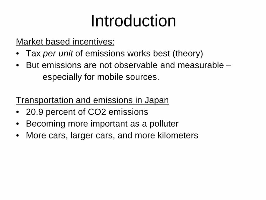
• Derived from Dubin-McFadden (1984)– Discrete choice (gas versus electricity)– Continuous choice (usage hours)

• Differences– Use three years of aggregate (average) data for 47

prefectures in Japan– Simultaneous estimation of the discrete choice (vehicles)

and continuous demand (distance).

Households• K types of vehicles including “no-car” option.• Direct utility

u(VKTI, ci)

iiii

g kycVKTKPL

pδ−=+

• Budget constraint

(1)

VKT= vehicle kilometers traveledKPL= fuel efficiency (kilometers per liter)pg = price of gasolinepi =pg /KPL price per kilometer in vehicle type ic = consumption goodd ki = annual capital cost of vehicle type i

• Indirect utility of choice i:

V( y-? ki, pi )

Parametric VKT demand, with log-linear specification:

ηγρβαα ++−++= ')()ln( 10 xkypVKT iiii (2) where ? is agent-specific unobserved characteristic. Rewrite as:

ηγρβαα ++−++= ∑∑ ')()ln( 10 xdkydpVKTj

ijjj

ijjji (3)

where dij = 1 if i=j; otherwise zero. The random error is correlated with dij. The conditional expectation E(?|bundle i) is not zero.

Taking expectation of (3), and add an additional iid random error, we have:

ij

jjj

jjji xSkySpVKT νγρβαα ++−++= ∑∑ ')()ln( **10 (4)

where S*

j is the predicted probability that jth bundle is chosen. Based on Roy’s identity, we can derive the indirect utility function:

( )( ) )exp(

1'exp

11

10 ii

iiii pxkyßaV α

αηγρ

β−−−−−−=

(5)

We use indirect utility to obtain probabilities of choosing each bundle.

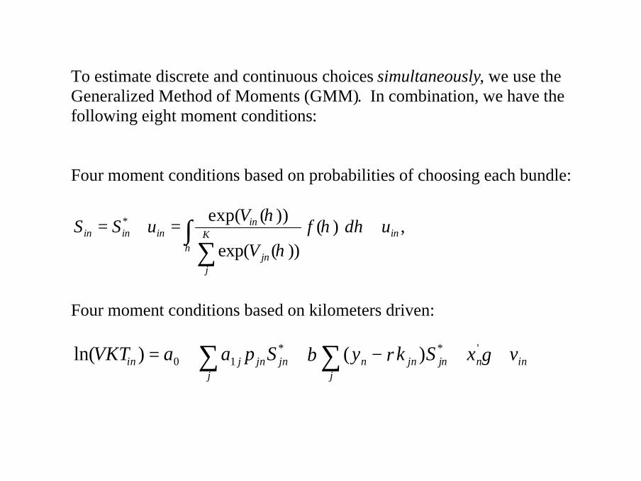
To estimate discrete and continuous choices simultaneously, we use the Generalized Method of Moments (GMM). In combination, we have the following eight moment conditions: Four moment conditions based on probabilities of choosing each bundle:

,)())(exp(

))(exp(*inK

jjn

inininin udf

V

VuSS +=+= ∫

∑ηη

η

η

η

Four moment conditions based on kilometers driven:

innj

jnjnnj

jnjnjin vxSkySpaaVKT ++−++= ∑∑ γρβ '**10 )()ln(

Data• Treat 47 Japanese prefectures as units of observation.• Vehicle bundles by size and vintage: {rn, ro, sn, so}

Sources

• Family Income and Expenditures Survey (2000-2002)• The 2000-2002 Population Census• Japan Automobile Dealers Association Automobile Statistics Data

Books (2000-2002)• The California Air Resources Board (1997, 2000)

– Fuel efficiency of vehicles (MPG) à obtain KPL– Estimates for “local” Emissions per mile (EPM) à obtain EPK– Estimates for Carbon-dioxide per mile (CPM) à obtain CPK

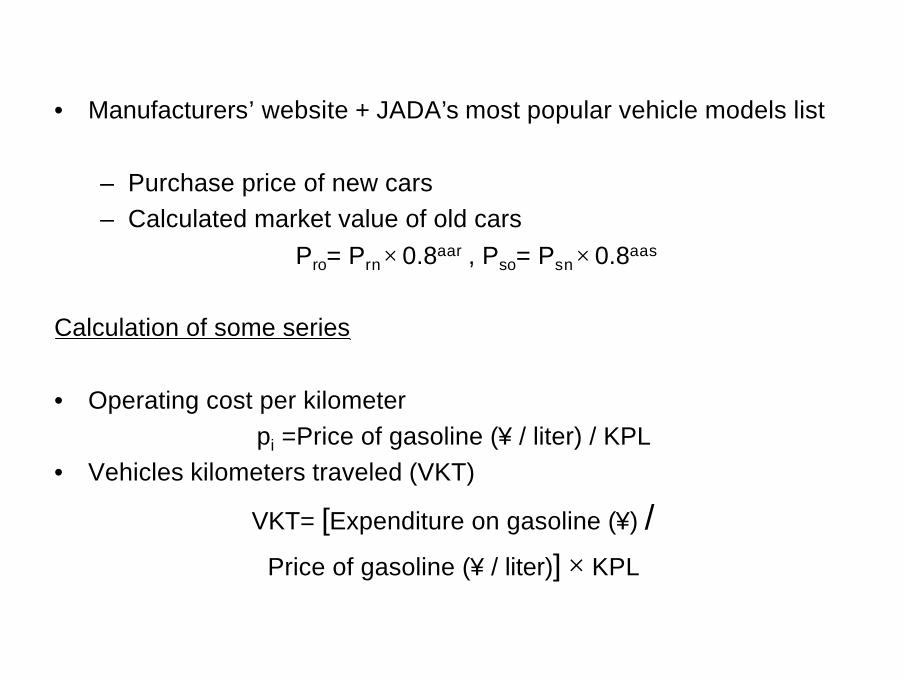
• Manufacturers’ website + JADA’s most popular vehicle models list

– Purchase price of new cars– Calculated market value of old cars

Pro= Prn × 0.8aar , Pso= Psn × 0.8aas

Calculation of some series

• Operating cost per kilometerpi =Price of gasoline (¥ / liter) / KPL

• Vehicles kilometers traveled (VKT)

VKT= [Expenditure on gasoline (¥) /Price of gasoline (¥ / liter)] × KPL

Table 1: Definitions and Summary Statistics

1,001,335(87,586)

Number of households in prefectureN

101.09 (0.267)Gasoline price (in ¥ per liter)Gasoline price

0.5139 (0.013)Yearly expenditure on gasoline (in ¥ 100,000)Gas Expenditure

37.57 (0.275)Yearly total expenditure (in ¥ 100,000)Y

0.655 (0.006)Homeowners fraction of householdsOwn-home

52.6 (0.133)Average age of the head of a householdAge

0.346 (0.005)Dual-income fraction of householdsTwo-earn

1.419 (0.012)Number of income earners per householdEarner

0.147 (0.001)Fraction of population less than 15 years oldChild

0.504 (0.016)Fraction residing in densely inhabited districts Metro

0.231 (0.005)Fraction of residents with higher educationEducationb

2.797 (0.018)Average number of people in a householdFamsize

Mean ValueVariable DefinitionVariable Name

Table 2: Estimation of Fuel Efficiency and Emission Rate

690.1440.00914(0.0027)

5.672(0.0357)

ln(CPM)Small-size cars

480.0006-0.0006(0.0122)

6.008(0.0413)

ln(CPM)Regular-size cars

Carbon Dioxide (CO2) Emission Rates

1380.4650.1176(0.0108)

-0.8850(0.1300)

ln(EPM)Small-size cars

960.6090.1480(0.0122)

-1.2067(0.1259)

ln(EPM)Regular-size cars

Emission Rates

1380.217-0.0128(0.0021)

3.382(0.0250)

ln(MPG)Small-size cars

960.083-0.0083(0.0029)

3.093(0.0293)

ln(MPG)Regular-size cars

Fuel Efficiency

Number of observations

R2AgeConstantDependent Variable

Table 3: Summary Statistics of the Choice-specific Variables

(0.022)(0.022)(0.029)(0.029)

9.748.648.1911.2610.88Gasoline cost (pi in ¥/km)

12.5643.43614.4627.70824.649Market value (ki in ¥100,000)

219.54191.64182.30251.79252.43CO2 emission rate (CPKi)

0.3640.5490.2880.4020.216Emission rate (EPKi)

10.58011.70312.3488.9759.294Fuel efficiency (KPLi)

(0.003)(0.002)(0.001)(0.000)

0.19650.4530.0810.2100.042Proportion choosing bundle i

MeanssosnrornChoices

EstimationInterpretation of our results:

• Higher price of gasoline, drive less.• Higher income (total expenditure), drive more.• More expensive vehicle, drive less.• For the same size car, a change in gas price per

kilometer has more influence on VKT in a new car than in an old car.

Table 4: Simultaneous Estimation of Discrete Choice and

Continuous Demand

[.000]33.348.765Constant for continuous choice (α0)

[.000] 5.8302.831Constant for choice four (α0so)

[.000] 11.435.455Constant for choice three (α0sn)

[.000] 14.116.920Constant for choice two (α0ro)

[.000]11.045.178Constant for choice one (α0rn)

[.000]-49.61-0.064Gas cost per kilometer of choice four (α1so)

[.000]-37.78-0.291Gas cost per kilometer of choice three (α1sn)

[.000]-65.78-0.211Gas cost per kilometer of choice two (α1ro)

[.000]-42.62-1.032Gas cost per kilometer of choice one (α1rn)

[.002]-3.034-0.0062Net income (β)

P-valuet-statisticParameterVariables

Table 4 (continued)

[.142]-1.470-0.034Dummy for Shikoku

[.000]3.7370.083Dummy for Chugoku

[.000]-4.567-0.110Dummy for Kinki

[.235]1.1870.030Dummy for Chubu

[.073]1.7950.050Dummy for Hokuriku

[.178]-1.348-0.031Dummy for Kanto

[.188]1.3180.028Dummy for Tohoku

[.000]6.7611.404Own-home

[.000]-4.504-0.014Age

[.000]3.742-1.005Two-earn

[.000]2.5790.130Earner

[.000]4.3433.383Child

[.000]-3.716-0.274Metro

[.000]-3.299-0.716Education

[.112]-1.587-0.102Famsize

Table 5: Estimated Own-Price and Cross-Price Elasticities of Each Choice with respect to gas cost (pi)

-2.7132.2492.2492.249pso

0.061-0.6940.0610.061psn

0.2190.219-0.8250.219pro

6.087E-66.087E-66.087E-6-1.389E-4prn

sosnrornChoicesPrices

Table 6: Estimated Own-Price and Cross-Price Elasticities of Each Choice with respect to capital cost (ki) and total expenditure (y)

-0.9091.038-0.766-0.876-0.717Total

expenditure (y)

0.0202-0.02430.02020.02020.0202kso

0.00110.0011-0.01270.00110.0011ksn

3.54E-43.54E-43.54E-4-0.00133.54E-4kro

0.00130.00130.00130.0013-0.0301krn

0(no car)

sosnrornChoicesCapital cost

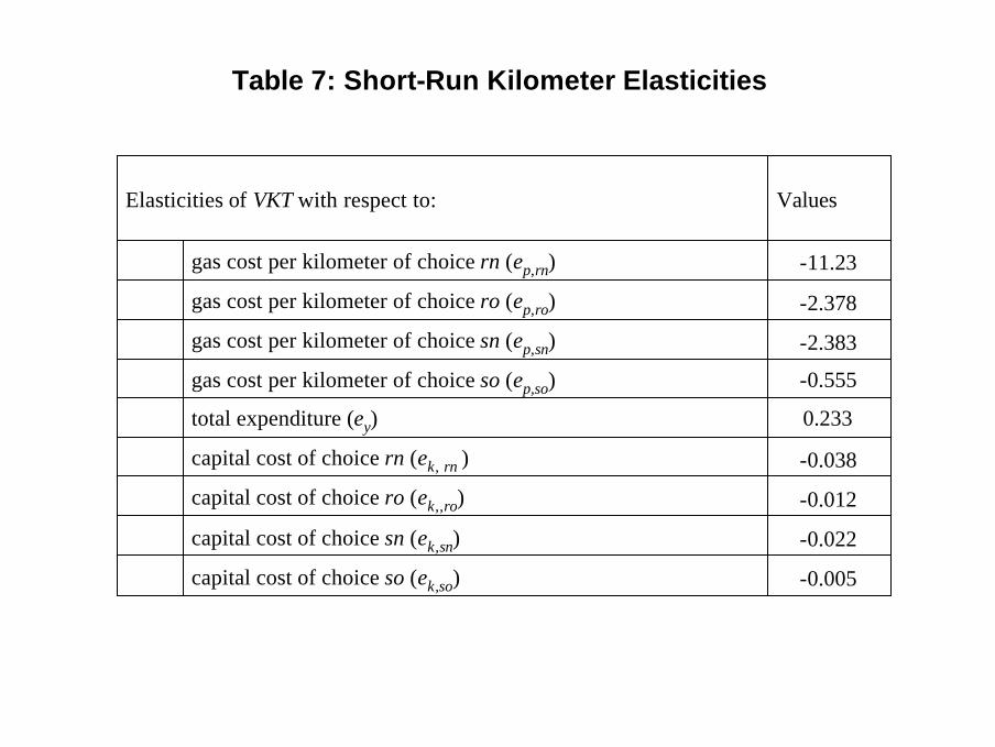
Table 7: Short-Run Kilometer Elasticities

-0.005capital cost of choice so (ek,so)

-0.022capital cost of choice sn (ek,sn)

-0.012capital cost of choice ro (ek,,ro)

-0.038capital cost of choice rn (ek, rn )

0.233total expenditure (ey)

-0.555gas cost per kilometer of choice so (ep,so)

-2.383gas cost per kilometer of choice sn (ep,sn)

-2.378gas cost per kilometer of choice ro (ep,ro)

-11.23gas cost per kilometer of choice rn (ep,rn)

ValuesElasticities of VKT with respect to:

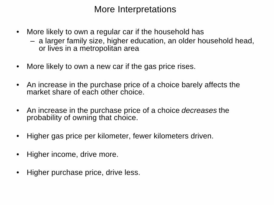
More Interpretations

• More likely to own a regular car if the household has– a larger family size, higher education, an older household head,

or lives in a metropolitan area

• More likely to own a new car if the gas price rises.

• An increase in the purchase price of a choice barely affects themarket share of each other choice.

• An increase in the purchase price of a choice decreases the probability of owning that choice.

• Higher gas price per kilometer, fewer kilometers driven.

• Higher income, drive more.

• Higher purchase price, drive less.

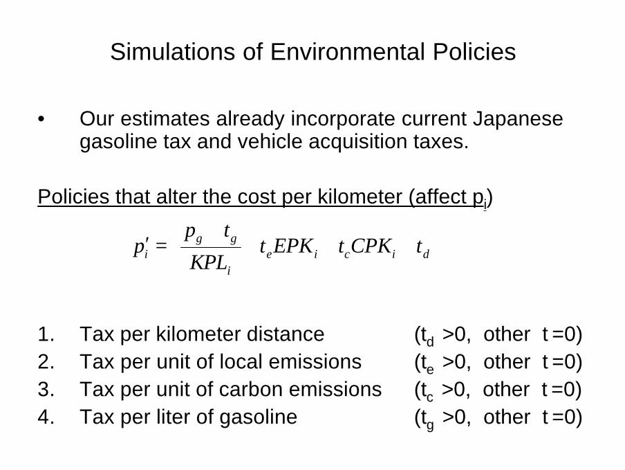
Simulations of Environmental Policies

• Our estimates already incorporate current Japanese gasoline tax and vehicle acquisition taxes.

Policies that alter the cost per kilometer (affect pi)

1. Tax per kilometer distance (td >0, other t =0)2. Tax per unit of local emissions (te >0, other t =0)3. Tax per unit of carbon emissions (tc >0, other t =0)4. Tax per liter of gasoline (tg >0, other t =0)

+++

+=′ dicie

i

ggi tCPKtEPKt

KPL

tpp

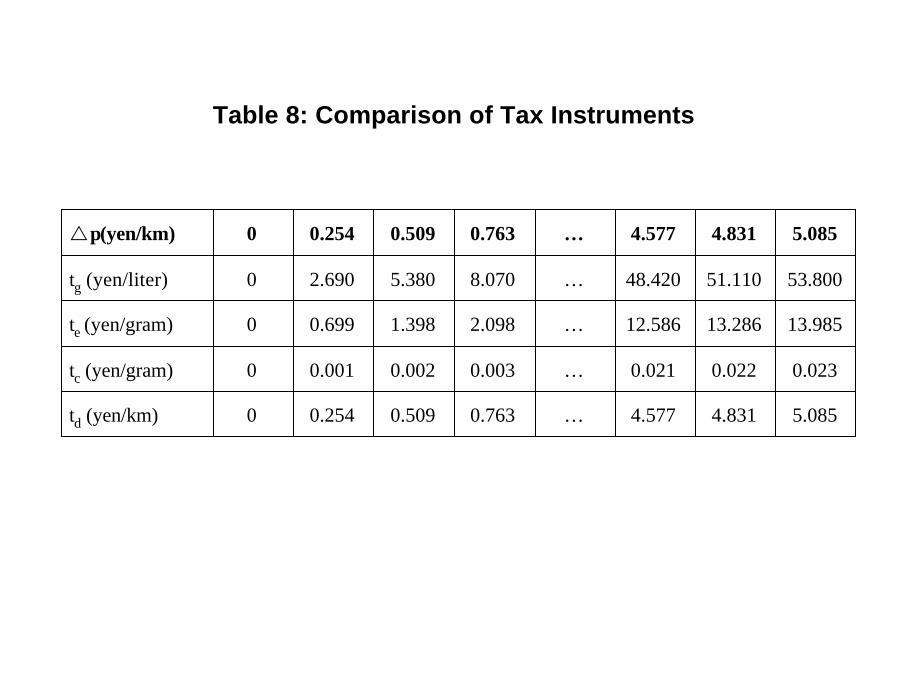
Table 8: Comparison of Tax Instruments

5.0854.8314.577…0.7630.5090.2540td (yen/km)

0.0230.0220.021…0.0030.0020.0010tc (yen/gram)

13.98513.28612.586…2.0981.3980.6990te (yen/gram)

53.80051.11048.420…8.0705.3802.6900tg (yen/liter)

5.0854.8314.577…0.7630.5090.2540rp(yen/km)

Figure 1: Effects of Four Policies on Vehicle-Kilometers Traveled (VKT)

-70

-60

-50

-40

-30

-20

-10

0

0.254

0.763

1.271

1.780

2.288

2.797

3.305

3.814

4.322

4.831

?p (yen/km)

% ?

in

VK

T

td

te

tc

tg

Figure 2: Effects of Four Policies on Local Emissions

-70

-60

-50

-40

-30

-20

-10

0

0.254

0.763

1.271

1.780

2.288

2.797

3.305

3.814

4.322

4.831

?p (yen/km)

% ?

in

Loca

l Em

issi

ons

td

te

tc

tg

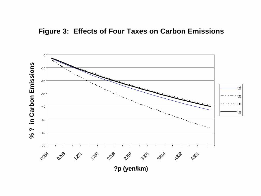
Figure 3: Effects of Four Taxes on Carbon Emissions

-70

-60

-50

-40

-30

-20

-10

0

0.254

0.763

1.271

1.780

2.288

2.797

3.305

3.814

4.322

4.831

?p (yen/km)

% ?

in

Car

bo

n E

mis

sio

ns

td

te

tc

tg

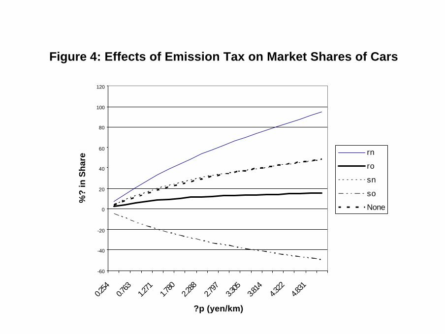
Figure 4: Effects of Emission Tax on Market Shares of Cars

-60

-40

-20

0

20

40

60

80

100

120

0.254

0.763

1.271

1.780

2.288

2.797

3.305

3.814

4.322

4.831

?p (yen/km)

%?

in S

har

e rn

ro

sn

so

None

Figure 5: Effects of Carbon Tax on Market Shares of Cars

-60

-40

-20

0

20

40

60

80

0.254

0.763

1.271

1.780

2.288

2.797

3.305

3.814

4.322

4.831

?p (yen/km)

%?

in S

har

e

rn

ro

sn

so

None

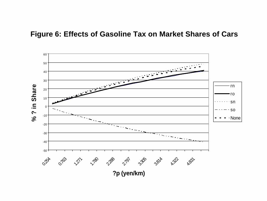
Figure 6: Effects of Gasoline Tax on Market Shares of Cars

-50

-40

-30

-20

-10

0

10

20

30

40

50

60

0.254

0.763

1.271

1.780

2.288

2.797

3.305

3.814

4.322

4.831

?p (yen/km)

% ?

in S

har

e rn

ro

sn

so

None

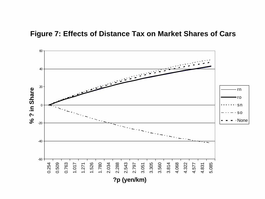
Figure 7: Effects of Distance Tax on Market Shares of Cars

-60

-40

-20

0

20

40

600.

254

0.50

9

0.76

3

1.01

7

1.27

1

1.52

6

1.78

0

2.03

4

2.28

8

2.54

3

2.79

7

3.05

1

3.30

5

3.56

0

3.81

4

4.06

8

4.32

2

4.57

7

4.83

1

5.08

5

?p (yen/km)

% ?

in S

har

e rn

ro

sn

so

None

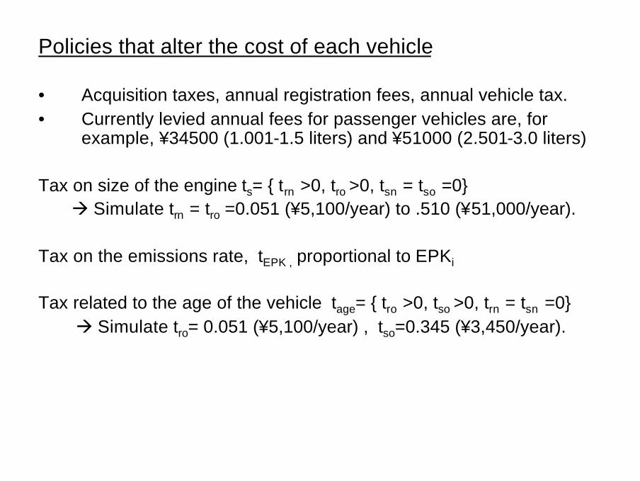
Policies that alter the cost of each vehicle

• Acquisition taxes, annual registration fees, annual vehicle tax.• Currently levied annual fees for passenger vehicles are, for

example, ¥34500 (1.001-1.5 liters) and ¥51000 (2.501-3.0 liters)

Tax on size of the engine ts= { trn >0, tro >0, tsn = tso =0}à Simulate trn = tro =0.051 (¥5,100/year) to .510 (¥51,000/year).

Tax on the emissions rate, tEPK , proportional to EPKi

Tax related to the age of the vehicle tage= { tro >0, tso >0, trn = tsn =0}à Simulate tro= 0.051 (¥5,100/year) , tso=0.345 (¥3,450/year).

Figure 8: Effects of Annual Size Tax on VKT, Carbon (CO2), and Local Emissions (LE)

-0.005

-0.005

-0.004

-0.004

-0.003

-0.003

-0.002

-0.002

-0.001

-0.001

0.000

0.051 0.102 0.153 0.204 0.255 0.306 0.357 0.408 0.459 0.510

0.051 0.102 0.153 0.204 0.255 0.306 0.357 0.408 0.459 0.510

Size Tax (Yen/year)

Per

cent C

han

ge

VKT

LE

CO2

trn

tro

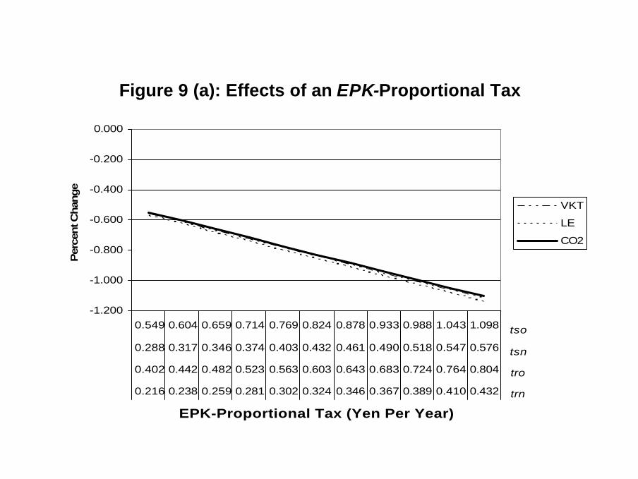
Figure 9 (a): Effects of an EPK-Proportional Tax

-1.200

-1.000

-0.800

-0.600

-0.400

-0.200

0.000

0.549 0.604 0.659 0.714 0.769 0.824 0.878 0.933 0.988 1.043 1.098

0.288 0.317 0.346 0.374 0.403 0.432 0.461 0.490 0.518 0.547 0.576

0.402 0.442 0.482 0.523 0.563 0.603 0.643 0.683 0.724 0.764 0.804

0.216 0.238 0.259 0.281 0.302 0.324 0.346 0.367 0.389 0.410 0.432

EPK-Proportional Tax (Yen Per Year)

Per

cent C

han

ge

VKT

LE

CO2

trn

tro

tsn

tso

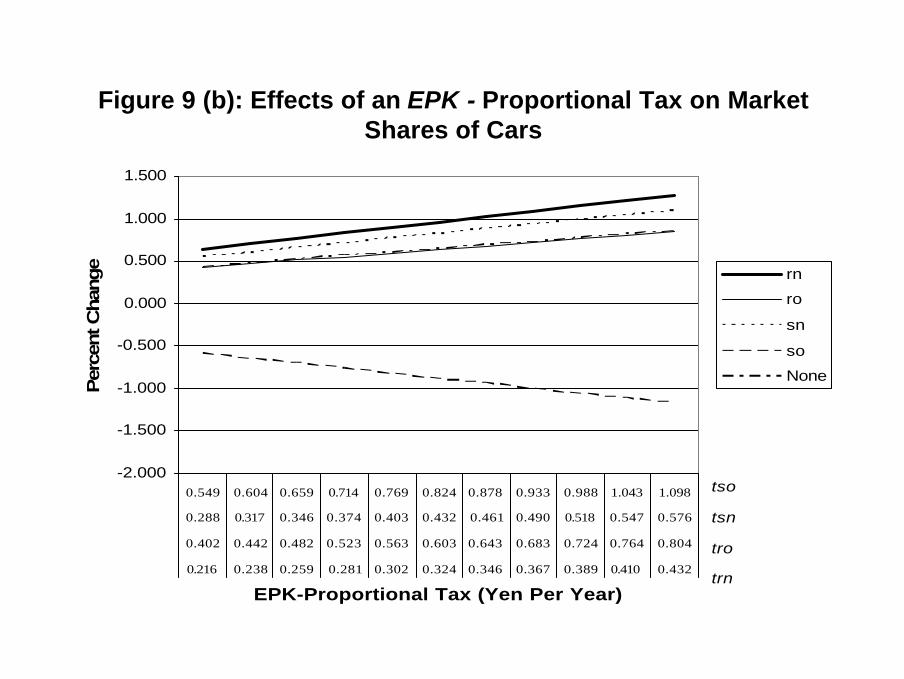
Figure 9 (b): Effects of an EPK - Proportional Tax on Market Shares of Cars

-2.000

-1.500

-1.000

-0.500

0.000

0.500

1.000

1.500

0.549 0.604 0.659 0.714 0.769 0.824 0.878 0.933 0.988 1.043 1.098

0.288 0.317 0.346 0.374 0.403 0.432 0.461 0.490 0.518 0.547 0.576

0.402 0.442 0.482 0.523 0.563 0.603 0.643 0.683 0.724 0.764 0.804

0.216 0.238 0.259 0.281 0.302 0.324 0.346 0.367 0.389 0.410 0.432

EPK-Proportional Tax (Yen Per Year)

Per

cent C

han

ge

rn

ro

sn

so

None

trn

tro

tsn

tso

Figure 10 (a): Effects of a Tax on Old Cars

-0.400

-0.350

-0.300

-0.250

-0.200

-0.150

-0.100

-0.050

0.000

0.000 0.035 0.069 0.104 0.138 0.173 0.207 0.242 0.276 0.311 0.345

0 0 0 0 0 0 0 0 0 0 0

0.000 0.051 0.102 0.153 0.204 0.255 0.306 0.357 0.408 0.459 0.510

0 0 0 0 0 0 0 0 0 0 0

AgeTax (Yen Per Year)

Per

cen

t C

han

ge

VKT

LE

CO2

tsn

tso

trn

tro

Figure 10(b): Effects of a Tax on Old Cars on Market Shares of Cars

-0.500

-0.400

-0.300

-0.200

-0.100

0.000

0.100

0.200

0.300

0.400

0.500

0.600

0.000 0.035 0.069 0.104 0.138 0.173 0.207 0.242 0.276 0.311 0.345

0 0 0 0 0 0 0 0 0 0 0

0.000 0.051 0.102 0.153 0.204 0.255 0.306 0.357 0.408 0.459 0.510

0 0 0 0 0 0 0 0 0 0 0

Age Tax (Yen Per Year)

Per

cent

Cha

nge

rn

ro

sn

so

None

trn

tro

tsn

tso

Figure 11: Marginal Cost of Abatement (MCA) for Local Emissions (HC, SO2, NOx)

0

5000

10000

15000

20000

25000

30000

0 50 100 150 200 250 300 350

Grams (Per Household Per Year)

MCA (Y

en P

er G

ram

)

Tg

Td

Te

Tc

Tage on car

Tem on car

Figure 12: Marginal Cost of Abatement (MCA) for Carbon Emissions (CO2)

0

20

40

60

80

100

120

0 50000 100000

Grams (Per Household Per Year)

MCA (Y

en P

er G

ram

)

Tg

Td

Te

Tc

Tage on car

Tem on car

Conclusions

• Developed a model of consumer behavior in Japan for – Discrete choice of vehicle bundle– Continuous choice of distance driven

• Unique use of prefectural data from Japan.• Simultaneous estimation of the model using GMM.• Logical effects of household income, car costs, and per-kilometer

costs on the household probability of each vehicle choice and on the choice of distance traveled.

• Policy alternatives induce different amounts of driving distancereductions and emission abatement.

Future Research

• Multiple policy instruments simultaneously.

– Welfare-maximizing rate for each instrument in use.– Prediction of costs, emissions, optimal tax rates.

• Analysis of distributional results of alternative policies

– Prediction of impact on low-income households– Calculation of all household EV and change in Gini.