A Model of Sliding-Scale Regulation1 - Ross School of …webuser.bus.umich.edu/tplyon/PDF/Published Papers/Lyon...Journal of Regulatory Economics; 9:227–247 (1996) ©1996 Kluwer

Journal of Regulatory Economics; 9:227–247 (1996)©1996 Kluwer Academic Publishers

A Model of Sliding-Scale Regulation1

THOMAS P. LYONUniversity of Chicago and Indiana University

School of Business, Bloomington, IN 47405

AbstractPrice caps, while widely touted, are less commonly implemented. Most incentive schemes involve profitsharing and are, thus, variants of sliding-scale regulation. I show that, relative to price caps, some degreeof profit sharing always increases expected welfare. Numerical simulations show that welfare may beenhanced by large amounts of profit sharing and by granting the firm a greater share of gains than oflosses. Simulations also suggest profit sharing is most beneficial when the firm’s initial cost is high andcost-reducing innovations are difficult to achieve but offer the potential for substantial savings.

1. Introduction

For years economists have complained about the woefully poor incentives created bytraditional rate-of-return regulation. Over the last decade, however, the institutional inno-vation of “price-cap regulation” has emerged, offering greatly enhanced incentives forefficient production and pricing.2 Nevertheless, many if not most of the “incentive regula-tion” plans implemented in recent years do not simply cap prices. Typically they also includelimits—-sometimes called “zones of reasonableness” or “deadbands”—-on how much thefirm can gain or lose before triggering profit-sharing with customers.3 Such regulatory

1 This paper has benefitted from the comments of Mark Bagnoli, Jim Burgess, Michael Crew, SteveHackett, Paul Kleindorfer, Michael Riordan, Ted Stefos, Ingo Vogelsang, Dennis Weisman, twoanonymous referees, and workshop participants at the First Annual Northeastern Health EconomicsConference, the Fourth Annual Health Economics Conference, GTE, Indiana University, the RutgersAdvanced Workshop in Regulation and Public Utility Economics, and the 20th TelecommunicationsPolicy Research Conference. Financial support from the Management Science Group of the Departmentof Veterans Affairs and from Indiana University is gratefully acknowledged.

2 Prominent examples in the United States include “price cap” regulation of AT&T by the FederalCommunications Commission (FCC) and fixed reimbursement payments for given diagnostic-relatedgroups under Medicare. A review of the extensive British experience with price caps is given byArmstrong, Cowan, and Vickers (1994).

3 The FCC’s original price-cap plan for the interstate access charges levied by the local exchange carriers(LECs), enacted in 1991, offered LECs a choice between two different earnings-sharing plans. After thefirst three years of this plan, the FCC revised the schemes and added a third plan that involves no sharing.For more details, see Sappington and Weisman (forthcoming). Over half the states in the United Stateshave adopted earnings sharing schemes, as discussed in detail by Greenstein, McMaster, and Spiller

schemes are known as ”sliding scale" (SS) plans. The recent enthusiasm for SS regulationhas been something of a mystery to economists, since it does not appear to reflect a newtheoretical case for its incentive effects. In fact, Braeutigam and Panzar (1993, 197) see SSregulation as “a classic case in which practice is far out ahead of theory” and note that (p.195) “[i]n view of the widespread and continuing implementation of [sliding-scale] plans,especially at the state level, a modern analysis of their effects on firm behavior and economicefficiency is long overdue.” This paper attempts such an analysis.

The model presented here provides a strong efficiency rationale for SS regulation. Theanalysis revolves around the interplay between the firm’s incentives for cost-reducinginnovation, the transaction costs of rate review, and the deadweight losses caused when pricesand costs are not properly aligned. A comparative institutional approach is taken, using amodeling framework that encompasses rate-of-return regulation, price caps, and sliding scaleregulation.4 SS regulation is seen as a flexible combination of the other two alternatives, withprofit-sharing used to balance the competing goals of providing incentives for cost reductionand of allowing price to track cost. The “deadband” reflects the high transaction costsassociated with rate reviews and allows these costs to be avoided when the benefits of priceadjustment are small. The results indicate that SS regulation, if properly designed, alwaysoffers greater welfare than pure price caps, which do not allow for price to adjust to cost expost. The optimal sharing rule often involves substantial refunds of profits to consumers andmay allow the firm to retain a greater share of gains than losses. The additional welfarebenefits of profit-sharing over pure price caps are greatest when the firm has high costs andwhen cost-reducing innovations are difficult to achieve but offer the potential for substantialsavings.

The remainder of the paper is organized as follows. Section 2 briefly surveys theliterature. Section 3 presents the basic model. Section 4 analyzes the benchmark cases ofcost-plus, rate-of-return, and price-cap regulation. Section 5 characterizes when sliding-scale regulation is welfare-enhancing relative to rate-of-return regulation and to price caps.Section 6 presents simulation results that extend the analytical results of section 5. Conclu-sions are offered in section 7.

2. Literature Review

The literature on profit-sharing is quite small.5 Greenstein, McMaster, and Spiller (1995)

228 THOMAS P. LYON

(1995). The prospective payment system (PPS) used by the Veterans’ Administration is designed so that ahospital cannot gain or lose more than 3% of its previous period’s budget. See Stefos, Lavallee, andHolden (1992, 5-6), for details. The California Public Utilities Commission (CPUC) has regulatedtransportation rates for some natural gas customers using what it calls a Negotiated Revenue StabilityAccount (NRSA) that “banded the effect that current incentive mechanisms could have on utilities’returns to a 300 basis point difference from the authorized level.’’ See California Public UtilitiesCommission (1990, 19-20). Indiana has recently enacted a scheme for PSI Energy that gives the companyall earnings below 10.6%, consumers all earnings beyond 12.3%, and uses a graduated sharing schedulebetween these two levels. See Indiana Utility Regulatory Commission (1990, 13).

4 Using a related framework, Cabral and Riordan (1989) and Clemenz (1991) study investment in costreduction under rate-of-return regulation and under price caps. Neither paper considers cost- orprofit-sharing, however, and their characterizations of rate-of-return and price-cap regulation differsignificantly from those used here, as discussed in footnote 10 below.

5 There is, of course, an extensive literature on optimal regulation under conditions of adverse selection,

study empirically how state regulators’ profit-sharing plans affect investment by localtelephone exchange companies. They find that price-cap plans offer stronger incentives forinvestment than do profit-sharing plans. Similarly, Majumdar (1995) measures the technicalefficiency of local exchange companies, finding that price caps induce greater efficiencygains than do profit-sharing plans. Since these studies ignore questions of allocativeefficiency, however, they cannot offer a welfare assessment of the respective plans.

There is also a theoretical literature that addresses the welfare effects of profit-sharingschemes. Sappington and Sibley (1992) find that small amounts of profit-sharing mayimprove welfare relative to some forms of price-cap regulation when investment is observ-able; this result becomes ambiguous, however, when investment is unobservable. Weisman(1993), in a multiproduct setting, shows that various distortions which result when commoncosts are allocated across products can be avoided by the use of price caps, but not by theuse of profit-sharing regulation. Gasmi, Ivaldi, and Laffont (1994) use numerical simula-tions to analyze profit-sharing for a monopolistic firm in an adverse selection setting withunobservable investment. They find that a deadband and profit-sharing are substitutes: eithera deadband is used and all earnings outside it are rebated to consumers, or there is nodeadband and profit sharing is employed. This dichotomy between regulatory plans bearslittle resemblance to the schemes used in practice, however, where deadbands and profitsharing appear to be complements rather than substitutes. Lyon (1995) shows that thecombination of a deadband plus profit-sharing can induce the efficient choice between aconventional technology and an innovative technology whose costs are lower in expectedvalue but higher in variance. Lyon and Huang (forthcoming) study incentives for theadoption of new technology when a firm under profit-sharing regulation competes with anunregulated firm. They find that, depending on the relative cost of innovation versusimitation, the industrywide rate of innovation may either speed up or slow down when theregulated firm is allowed to keep a larger share of profits.

This paper differs from the theoretical papers discussed above in several ways. UnlikeSappington and Sibley (1992), I focus on unobservable cost-reducing investment that hasnon- deterministic effects and on linear pricing schemes. I also use simulation analysis toinvestigate degrees of profit-sharing that depart significantly from price caps. UnlikeWeisman (1993), I study a single-product firm in order to focus on the case where costs areuncertain and profits are returned to customers via price reductions rather than lump-sumtransfers. Unlike Gasmi, Ivaldi, and Laffont (1994), the model presented here is fundamen-tally one of moral hazard, or hidden action, rather than hidden information.6 Both types ofmodel capture important aspects of reality, and the choice between them reflects beliefs aboutthe relative importance of effort provision versus information revelation, as well as their

A MODEL OF SLIDING-SCALE REGULATION 229

much of which emphasizes the sharing of costs between the regulator and the firm. For a thoroughtreatment, see Laffont and Tirole (1993). Schmalensee (1989) analyzes a model in which price is a linearfunction of cost and provides a variety of interesting simulation results.

6 In the latter family of models, the principal typically distorts pricing behavior in subtle ways in order tominimize the informational rents earned by the agent possessing private information. Moral hazardmodels, on the other hand, usually trade off incentives for greater effort—generated by giving the agent agreater claim to residual surplus—against the cost such claimancy imposes on the risk-averse agent whenoutcomes are stochastic. My model differs from the typical moral hazard setup in that the firm isrisk-neutral and allocative efficiency substitutes for risk-aversion as the brake on the use of high-poweredincentives.

ability to explain and predict behavior. One appealing aspect of my simple model is that itprovides a clear explanation for the complementary use of deadbands and profit sharing,which Gasmi et al. (1994) do not. This paper also differs from Gasmi et al. (1994) in that itreturns excess earnings to consumers via price reductions (as is typically done in practice)rather than lump-sum transfers, and it does not impose ex post limited liability, so both thesharing of gains and of losses is allowed. The basic structure in the present paper is similarto that in Lyon (1995), but the earlier paper focuses on a positive analysis of the regulatedfirm’s choice between discrete technological alternatives, while the current paper takes abroader view of social welfare that trades off productive and allocative efficiency. Finally,this paper differs from Lyon and Huang (forthcoming) in its focus on optimal profit-sharingrules for a regulated monopolist.

3. The Basic Model

In this section, I present a stylized model of firm behavior under regulation. The firm caninvest in innovative efforts to reduce costs, the success of which cannot be predictedperfectly. Examples of such investments might include research and development, changesin the way the firm is organized, or the adoption of new production techniques. Regulatorsare assumed to be unable to observe the firm’s effort directly.

The regulatory process as modeled here is motivated by an underlying process of interestgroup politics. As is well known, under Supreme Court decisions such as Munn v. Illinois,states can regulate profits in industries “affected with a public interest;” similarly, firms areentitled, under Federal Power Commission v. Hope Natural Gas, to seek rate increases whenprofits are low. As emphasized by Joskow (1974) and Peltzman (1976), however, interestgroups wishing to affect the political process must incur the transaction costs of acquiringinformation and organizing for action; thus, interest group pressure for rate review tends toemerge only when economic conditions diverge significantly from those at the last review.

More formally, consider a risk-neutral single-product firm with constant marginal andaverage production cost c. Its initial cost is c0, but this can be reduced, albeit with someuncertainty, depending on the amount e the firm expends on cost-reduction activities. Thereis thus a probability density function f(c e) with cumulative F(c e) that relates cost toeffort. I assume F(0,e) = 0, F(c0 e) = 1, and that cost-reducing effort is subject to decreas-

ing returns, i.e., Fe(c e) ≥ 0 ≥ Fee(c e). Both the regulator and the firm have access tohistorical data on prices and sales, but while the firm chooses e, the regulator cannot observeit. Let ψ(e) represent the firm’s disutility of effort, with ψ′(e) > 0 and ψ′′(e) > 0.

I follow Banks (1992) in assuming that the firm’s costs and earnings are observable butcan only be verified for rate-making purposes by holding a formal rate review, which entailssocial costs of ∆.7 At any point in time, the price from the most recent rate review, p0, remainsin effect unless a new rate review is held.

The basic price adjustment mechanism in this model is quite simple. An initial price p0

is set less than or equal to the most recent observation of average (and marginal) cost, c0.

Given p0, the firm’s earnings gross of cost-reduction expenses are R(c) ≡ [p0 − c]q(p0), and

230 THOMAS P. LYON

7 The costs of the firm, consumer groups, and regulatory staff are all included in ∆.

net of cost-reduction expenses are R(c) − ψ(e). The price remains unchanged as long asearnings remain within the “deadband,” i.e., between a lower bound L and an upper boundU. These upper and lower bounds are shaped by the cost to interest groups (the firm andconsumers, respectively,) of mobilizing to participate in the regulatory process. IfR(c) ∉ [L,U], then any gross earnings outside the deadband are shared between ratepayers

and shareholders, with αL the firm’s share of gross earnings below the deadband and αU thefirm’s share of gross earnings above the deadband. Thus, allowed profits are

π(c e) =

L + αL[R(c) − L] − ψ(e)R(c) − ψ(e)U + αU[R(c) − U] − ψ(e)

if R(c) < L

if R(c) ∉ [L,U]

if R(c) > U.

(1)

I assume the regulator is unable to make use of lump-sum transfers and can only adjustprofits by changing the output price p.8 Thus, when R(c) > U, the regulator sets a new price

p so that the new revenue requirement is 5 (c) = U + αU[R(c) − U] = αUR(c) + (1 − αU)U.

The price, pU, that achieves this objective is found by setting (pU − c)q(pU) =αU(p0 − c)q(p0) + (1 − αU)U. A similar procedure applies for R(c) < L. It is not possible ingeneral to obtain a closed-form solution to this pricing problem, although a solution can befound for specific demand functions.

The above structure captures as special cases several familiar regulatory schemes:

• Cost-plus (CP) regulation: L = U = 0, αU = αL = 0. Price, ex post, is always set equalto observed marginal cost.

• “Pure” price-cap (PC) regulation: αU = αL = 1. Price is set at an initial level p0 ≤ c0

and remains unchanged regardless of observed marginal cost.

• Rate-of-return regulation (RORR): 0 = L < U, αU = αL = 0.9 An initial price p0 = c0 isset and remains in place unless earnings are too high or too low. If earnings are toohigh, the firm reduces prices to avoid consumer outrage; if earnings are too low, thefirm petitions for rate review and has price reset so as to just cover costs.10

In addition, the pricing rule described above allows for the more flexible structures beingimplemented in the industries mentioned above. Throughout the paper, I assume no “drastic”

innovations are possible, i.e., even if cost is zero, the monopoly price pM(0) is at least p0.11

A MODEL OF SLIDING-SCALE REGULATION 231

8 Schmalensee (1989) discusses this point at length.9 See Braeutigam and Quirk (1984) for further discussion of this model of rate-of-return regulation.10 There is some disagreement in the literature as to how rate-of-return regulation and price-cap regulation

should be characterized. Schmalensee (1989) uses the static characterizations of cost-plus regulation andprice-cap regulation given above; he does not explicitly model rate-of-return regulation. Cabral andRiordan (1989) and Clemenz (1991) model rate-of-return regulation as holding rate reviews at fixedintervals and price caps as allowing the firm to petition for a rate increase if and when it so chooses. Pint(1992), on the other hand, portrays RORR as giving the firm the right to initiate rate review, while underPC regulation reviews are held at fixed intervals. The empirical work of Joskow (1974) and Fitzpatrick(1987) supports the notion that traditional rate-of-return regulation gives the firm considerable power tomanipulate the timing of rate reviews and, thus, comports with the modeling of Pint and of the presentpaper.

Define cU = p0 − U ⁄ q(p0) and cL = p0 − L ⁄ q(p0) as the cost levels at which the firm’searnings hit the upper and lower bounds on profits respectively. Then the relationshipbetween price and cost for the three benchmark cases is as shown in figure 1.

The firm’s expected profits can be written as

π__

(e) = ∫ 0

cU

[(1 − αU)U + αU(p0 − c)q(p0)]dF(c e) + ∫ c

U

cL

(p0 − c)q(p0)dF(c e)

+ ∫ c

L

c0[(1 − αL)L + αL(p0 − c)q(p0)]dF(c e) − ψ(e). (2)

Totally differentiating the firm’s first-order condition with respect to effort, it is easy to

show that de ⁄ dL ≤ 0, de ⁄ dU ≥ 0, de ⁄ dαL ≥ 0, and de ⁄ dαU ≥ 0. The intuition for the signson these terms is straightforward: the firm increases its cost-reducing effort when it appro-priates a greater share of the benefits of effort. This greater appropriation occurs if the upper(lower) bound on earnings is raised (lowered) or if the firm receives a larger share of anyearnings beyond U or L.

Since price is a function of cost, expected consumer surplus is S_ = ∫

0

c0S(p(c))dF(c e) or,

more explicitly,

S_ = ∫

0

cU

S(pU)dF(c e) + S(p0)[F(cL,e) − F(cU,e)] + ∫ c

L

c0

S(pL)dF(c e). (3)

Figure 1. Pricing for Three Benchmark Cases

232 THOMAS P. LYON

11 As the term is used in the literature, a “drastic” innovation is one which so lowers the cost of productionthat the monopoly price, based on the new cost, is below the original cost. If a firm in a competitiveindustry developed a drastic innovation, it would thus drive all its rivals out of business.

Total surplus (which I will refer to as “welfare”) is W__

= S_ + π

__ and will be the focus of

much of the analysis to follow. Many normative models of regulation give profits astrictly smaller weight in regulatory objectives than consumer surplus. In a moralhazard model such as the one presented here, however, the weight placed on profits isrelatively unimportant, since welfare maximization drives the firm to its reservationlevel, here assumed to be zero expected profits. Thus, only Proposition 4 of the paperwould be affected if profits were weighted less than consumer surplus; these changesare discussed explicitly after the proposition is presented.

Differentiating expected consumer surplus with respect to αU yields

dS_

dαU = ∂S_

∂αU + ∂S_

∂e

de

dαU . (4)

The first term (the “allocative effect”) is always negative, since it requires priceincreases to consumers. The second additive term (the “incentive effect”) is positive.

As mentioned above, de ⁄ dαU ≥ 0. Integrating (3) by parts and partially differentiatingwith respect to e yields

∂S_

∂e = ∫

0

cU

q(pU) dpU

dc Fe(c e)dc + ∫

cL

c0q(pL) dpL

dc Fe(c e)dc.

It can be shown that dpU ⁄ dc > 0 and that if L ≤ 0 then dpL ⁄ dc > 0. Thus, if L ≤ 0, then

∂S_

⁄ ∂e > 0, and the incentive effect of αU on consumer surplus is positive. Similar

expressions can be derived for αL.

4. Benchmark Cases

I next examine the performance of the three benchmark regulatory systems outlinedabove.

4.1. Cost-Plus RegulationPure cost-plus (CP) regulation has αL = αU = 0 and L = U = 0, so that p = c ex post.

Because the firm’s cost-reducing effort is unobservable, these costs are never recovered inrates and π

__(e) = − ψ(e). The firm has no incentive to reduce its costs and e∗ = 0. As a result,

price does not fall, expected profits are zero, and consumer surplus is governed entirely bythe initial regulated price, e.g., S

_(e∗) = S(p0). This form of regulation has received much

public condemnation, but it is essentially a caricature. Authors such as Joskow andSchmalensee (1986) have discussed at length why traditional rate-of-regulation differs froma simple cost-plus format.

4.2. Rate-of-Return RegulationTraditional rate-of-return regulation (RORR) is characterized by p0 = c0, 0 = L < U, and

αL = αU = 0. Then (2) becomes

A MODEL OF SLIDING-SCALE REGULATION 233

π__

(e) = ∫ 0

cU

UdF(c e)dc + ∫ c

U

c0(p0 − c)q(p0)dF(c e) − ψ(e). (6)

Integrating by parts and differentiating with respect to effort, the firm’s first-order conditionbecomes

dπ__

de = q(p0)∫

cU

c0

Fe(c e)dc − ψ′(e) = 0. (7)

The presence of the “deadband” means that RORR induces a positive level of effort and,thereby, generates lower expected costs than cost-plus regulation. Furthermore, both thefirm and consumers are better off than under CP regulation. The deadband allows the firmto keep some of the benefits of cost reduction, while consumers benefit because prices willbe reduced for sufficiently large cost reductions.12 These benefits are even greater when thetransaction costs of rate review are recognized: the deadband economizes on the transactioncosts of rate review when costs have changed little since the last rate review.

4.3. Price CapsPure price-cap (PC) regulation has αL = αU = 1, so p = p0 ex post regardless of cost.

(Because I assume pM(0) > p0, downward price flexibility makes no difference.) Thus,

equation (2) reduces to π__

(e) = ∫ (p00

c0 − c)q(p0)dF(c e) − ψ(e), and, after integrating by

parts, the firm’s first-order condition is

dπ__

de = q(p0) ∫

0

c0Fe(c e)dc − ψ′(e) = 0.

(8)

Obviously, S_

(e∗) = S(p0). Thus, under pure price caps, consumers do exactly as well as theydo under cost-plus regulation if the same initial price p0 is used in both regimes. The firm,however, makes greater profits under price caps. The regulator can thus set the initial pricecap lower than c0 and capture for consumers some of the benefits of cost reduction. This isdemonstrated in Lemmas 1 and 2 below.

Lemma 1. Under pure price cap regulation, (a) there exists a price p_ below which expectedprofit is negative. (b) For p0 > p_, de ⁄ dp < 0.

Proof: See Appendix. Q.E.D.

Lemma 1 shows that lowering the initial price induces greater effort as long as the priceis above p_.13 Lemma 2 characterizes the social-welfare maximizing price under pure

234 THOMAS P. LYON

12 Note that the deadband plays a role similar, but not identical, to that of regulatory lag in dynamic modelsof regulation. The time period between rate reviews is driven by two components. First, because of thetransaction costs of triggering a rate review, such a review will not be triggered until economic conditionsdepart significantly from those at the last review. Second, once review is triggered, there is a “processinglag” that reflects the time delays inherent in legal adjudication. The present paper reflects only the first ofthese aspects of regulatory lag.

price-cap regulation.

Lemma 2. Under pure price-cap regulation, if expected profits are kept non-negative,welfare is maximized at p0 = p_.

Proof: Let W__

∗(p0) and π__

∗(p0) be expected welfare and expected profits respectively at thefirm’s optimal level of effort. It is straightforward to show that

dW__

∗(p0)dp0

= q′(p0)π__

∗(p0)q(p0)

. (9)

For any price cap that leaves π__

∗(p0) ≥ 0, welfare is decreasing in price. Welfare is

thus maximized at p0 = p_. Q.E.D.

It follows immediately that since p_ < c0, price caps can be designed so as to Pareto-dominatecost-plus regulation.14 The effort level and expected cost induced by PC are compared tothose under RORR and CP regulation in Proposition 1.

Proposition 1. The firm’s effort under price-cap regulation is greater than that underrate-of-return regulation, which is greater than that under pure cost-plus regulation.The firm’s expected cost under price-cap regulation is less than that under rate-of-return regulation, which is less than that under pure cost-plus regulation.

Proof: See the Appendix. Q.E.D.

Proposition 1 is quite consistent with intuition. Price caps are designed to maximize effortby inducing the firm to act as a price taker. Cost-plus regulation induces no effort, since thefirm cannot recover its cost of effort. Finally, RORR involves rigid prices in the short run,is cost-plus in the long run, and thus is intermediate between cost-plus and price capregulation.15 Not surprisingly, then, the firm’s choice of effort under RORR is between thatunder cost-plus and price caps.16

While it is possible to rank the above schemes in terms of the effort they induce, welfarecomparisons are ambiguous. Under RORR, (3) can be integrated by parts to yield

S_ = S(p0) + ∫

0

cU

q(pU) dpU

dc F(c e)dc. (10)

Because dpU ⁄ dc > 0, RORR generates greater consumer surplus than does pure PC regula-tion, assuming the same initial price p0 = c0. RORR offers consumers two benefits: first, itadjusts price closer to marginal cost when profits rise “too” high, and second, because

A MODEL OF SLIDING-SCALE REGULATION 235

13 The results of Lemma 1 are similar to those of Cabral and Riordan (1989) in their Propositions 3.1 and3.2, but Lemma 1 applies for all p0, not just p0 = c0.

14 Because welfare-maximization requires expected profits be set to zero, the weight on profits in the welfarefunction has no impact on Lemma 2.

15 Joskow and Schmalensee (1986) discuss this point extensively.16 Despite our different modeling of RORR and PC regulation, this result parallels Proposition 4.1 of Cabral

and Riordan (1989).

p0 = c0, there is no possibility of costs above c0, so a sharing rule never forces consumers tobear responsibility for negative profit outcomes.17 However, if the price-cap scheme beginswith an initial price p0 < c0—and this is clearly the intent of price-cap regulation—thecomparison is in general ambiguous.18

5. Sliding-Scale Regulation

This section examines the performance of sliding-scale regulation relative to RORR and toprice caps. It is assumed throughout that L ≤ 0 and U ≥ 0. A complete characterization isnot possible using analytical techniques, but marginal shifts away from RORR or PC andtoward SS are examined in Propositions 2 and 3. Proposition 4 shows that profit-sharing,implemented via lump-sum transfers, never produces greater total surplus than price caps.In addition, Proposition 5 provides sufficient conditions for a deadband to be a welfare-im-proving part of SS regulation.

Proposition 2 addresses the question of whether profit-sharing improves upon rate-of-re-turn regulation.

Proposition 2. Relative to rate-of-return regulation, a small increase in αU increases welfarefor small enough U; for large U the welfare effects of profit-sharing are ambiguousin general.

Proof: See the Appendix. Q.E.D.

Proposition 2 shows that profit-sharing is welfare- increasing for small enough U. Thisis easy to understand because as U becomes small, RORR approaches cost-plus regulation,which provides no incentive for effort. In this situation, the allocative distortions caused by

setting αU > 0 are swamped by the beneficial incentive effects.19 The next propositionaddresses the shift from PC to SS.

Proposition 3. Relative to pure price-cap regulation, welfare can always be increased

through a small decrease in αL and a small decrease in αU, which jointly leaveexpected profits unchanged.

Proof: See the Appendix. Q.E.D.

Proposition 3 establishes conditions under which profit-sharing enhances welfare relative

236 THOMAS P. LYON

17 In practice, price-cap regulation allows for price reduction if the firm’s costs are so low that the monopolyprice is below p0. (This of course will never happen if drastic innovations are impossible.) As long as theupper bound U on profits is below the monopoly profit level, consumers will experience price reductionsin more states of the world under RORR than under price caps.

18 This ambiguity, which parallels the results of Schmalensee (1989), reflects the idea that a price capsacrifices price flexibility to achieve stronger incentives. My model thus differs sharply from that ofClemenz (1991), who concludes that PCs can always be designed so as to produce higher welfare thanRORR. The main reason is that Clemenz’s “price caps” have upward price flexibility. See footnote 10for further discussion of our respective assumptions.

19 For U close to zero, this result holds regardless of the weighting of profits in the welfare function. Anincrease in αU always increases profits. Furthermore, as U goes to zero, any increase in incentives mustbenefit consumers as well, since otherwise they have no hope of a price reduction.

to pure price caps.20 The basic notion is simple: when αU = αL = 1, sharing produces afirst-order allocative gain, but only a second-order loss in the form of weakened incentives.21

It is also worth pointing out that welfare is not increased by adding profit-sharing to aprice-cap scheme if profits are returned to customers as a lump sum. This is shown inProposition 4.

Proposition 4. Relative to pure price cap regulation, profit-sharing with benefits distributedto consumers through lump-sum transfers reduces welfare.

Proof: Consider pure PC regulation with some initial price p0. While lump-sum transfersex post have no impact on total welfare, any transfer of profits away from the firmreduces its cost-reducing effort, raising expected costs and reducing expectedwelfare. Welfare losses are exacerbated if price must be increased to keep expectedprofits non-negative. Q.E.D.

Proposition 4 provides a rationale for why profit-sharing schemes commonly refundshared earnings to customers via price reductions rather than lump-sum transfers. Note,however, that it need not hold if profits receive little weight in the welfare function, since ifprofit is unimportant, pure transfers from the firm to consumers raise welfare. Similarly,transfers to particular favored groups of customers might be desired by regulators. Suchregulatory preferences may explain the provisions in some state regulations that requireshared earnings to be invested in network modernization for specific customer groups.22

Finally, I return to the question of the welfare effects of a deadband. In section 4, it waseasy to see that the deadband embedded in RORR improves upon pure cost-plus regulation,since it both enhances the firm’s incentive to exert effort and economizes on regulatory costsin situations where costs have changed little since the last rate review. Proposition 5examines the welfare effects of a deadband in the more general case where profit-sharing isallowed. Let ∆ be the transaction costs of a rate review; this would include, for example, theorganizational costs of consumers, the fees of lawyers and consultants, and the opportunitycost of allocating some of the firm’s employees to rate case preparation. Total welfare isnow

W__

= S_ + π

__ − ∆[1 − F(cL e) + F(cU e)]. (11)

Proposition 5. A deadband, i.e., a pair of parameters L and U with L ≤ 0 ≤ U, where at leastone of the inequalities is strict, enhances welfare if the demand curve is downward-sloping and the transaction costs of rate review are large enough.

Proof: See the Appendix. Q.E.D.

Proposition 5 shows that the allocative distortions created by a deadband must be balancedagainst the enhanced incentives and the reduced transaction costs the deadband provides.

A MODEL OF SLIDING-SCALE REGULATION 237

20 Because the proposition requires expected profit to remain unchanged, it is clearly not affected by theweight of profits in the welfare function.

21 Proposition 3 is similar to Findings 6 and 7 in Sappington and Sibley (1992), though those authors do notallow for a deadband and they require αL = αU. In both models, however, the key is that profit-sharingimproves allocative efficiency.

22 See Greenstein et al. for details on the various plans.

As long as the demand curve is downward-sloping, allocative distortions are bounded, so adeadband enhances welfare if ∆ is large enough. Even if ∆ = 0, a deadband might enhancewelfare if the resulting allocative distortions are smaller than the incentive effects; this mighthappen, for example, if c0 is small enough that the allocative effects of loss-sharing areminor.23

To summarize the key results of this section, profit-sharing cannot necessarily improveupon rate-of-return regulation, but it can always offer an improvement over pure price caps,assuming profit-sharing is implemented via price changes. Furthermore, a deadband is awelfare-enhancing component of SS regulation if the transaction costs of rate review arelarge enough. These results are limited, however, since they only address marginal changesin the amount of profit-sharing. To obtain further insight into the effects of large changesin the extent of profit-sharing, the following section presents the results of a numericalsimulation analysis.

6. Simulation

This section reports results of a numerical simulation of the foregoing model of sliding-scaleregulation. Its purpose is two-fold: 1) To examine whether sharing rules that are significantly

different from αL = αU = 1 can improve welfare relative to pure price caps, and 2) To studythe relationship between changes in exogenous parameters and changes in the welfare-maxi-mizing values of the choice variables.

The simulation uses a linear demand function q = 10 − p, with ψ(e) = e2, and considers arange of initial cost levels from c0 = 1 to c0 = 9.24 The probability distribution on costs is

F(c e) = 1 − 1 −

cc0

de

,

with corresponding density function

f(c e) = dec0

1 −

cc0

de − 1

and likelihood ratiofe(c e)f(c e)

= 1de

+ ln 1 −

cc0

.

This density function generates an expected value of cost

c_(e) =

c0

de + 1 .

Thus, d is a measure of the efficiency of the cost-reduction technology. The cumulative

238 THOMAS P. LYON

23 Note that the proposition continues to hold if profit receives a low weight in the welfare function, sincethe deadband retains its important role in reducing transaction costs.

24 The costs of rate review are not included in the simulation, so a deadband is not examined.

distribution is shown in figure 2 for several alternative effort levels.25 It has the appealingproperties that, if the firm exerts no effort then cost is c0 with certainty, and that expectedcosts decline monotonically with effort.

Price Cap RegulationThe optimal pure price cap p_ is shown in figure 3 for various levels of initial average cost

Figure 2. Probability Distribution on Costs for Alternative Effort Levels

Figure 3. Optimal Price Caps for Various Cost-Reduction Efficiencies

A MODEL OF SLIDING-SCALE REGULATION 239

25 Note that the distribution satisfies both the monotone likelihood ratio property and the convexity of thedistribution function condition discussed in Rogerson (1985). These two conditions are commonly usedin agency models.

c0 and efficiency of cost reduction d. While the cap increases with c0, dp_ ⁄ dc0 is well below

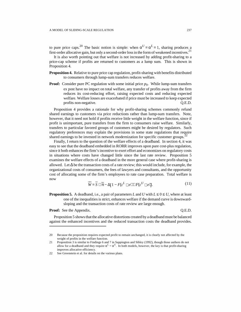
1 for all cases examined. In addition, the slope dp_ ⁄ dc0 diminishes as the cost-reductiontechnology becomes more efficient, i.e., as d increases. The corresponding levels of totalwelfare are shown in figure 4. As one would expect, welfare increases with the efficiencyof the cost-reduction technology. An efficient technology also helps offset the welfare-re-ducing effect of a high initial cost.

Sliding-Scale Regulation A major purpose of the simulation is to study the characteristics of welfare-maximizing

profit-sharing rules. The approach taken here was to first solve for the optimal pure pricecap and then, holding the price cap fixed, solve for the welfare-maximizing sharing levels.26

It should be noted from the outset that monotonic relationships between the level of profitsharing and exogenous parameters such as c0 and d cannot be expected. Milgrom andShannon (1994) provide necessary and sufficient conditions for such monotone comparativestatics to emerge, and these conditions are not met in my model of sliding-scale regulation.27

Figure 4. Welfare under Optimal Price Caps

240 THOMAS P. LYON

26 This procedure was adopted primarily to reduce the computational burden of the simulations. Preliminarytests indicated the optimal price level was very insensitive to the presence of profit sharing. Gasmi et al.(1994) also found that the introduction of profit sharing typically has little impact on the optimal pricelevel.

27 The two conditions are: 1) the objective function is supermodular in the choice variables, and 2) theobjective function has increasing differences in the choice variables and the exogenous parameters. Forsmooth functions in 5N, these conditions simplify to restrictions on the cross-partial derivatives of theobjective function. In my model, both conditions fail because ∂2W/∂αU∂p0 and ∂2W/∂αU∂c0 areambiguous in sign.

The firm’s share of gains and losses under welfare-maximizing SS regulation is shownin figures 5 and 6 for various levels of c0 and d. Several observations are worthy of note.

First, in all cases examined, the firm’s share of gains, αU, is greater than its share of losses,

αL; hence, the profit function is convex in observed cost. This convexity may help inducethe firm to undertake the risks of investing in cost reduction. Second, loosely speaking, the

Figure 5. Welfare-Maximizing Sharing Rules (d = 1, L = U = 0)

Figure 6. Welfare-Maximizing Sharing Rules (c0 = 5, L = U = 0)

A MODEL OF SLIDING-SCALE REGULATION 241

welfare-maximizing values of αL and αU decline with increases in c0, though the decline iscertainly not monotonic. With higher initial cost, there is a wider range of possible ex postcost levels, and hence price flexibility is more important. Third, loosely speaking, the

welfare-maximizing values of αL and αU rise with increases in d, though again the declineis not monotonic. A more efficient cost-reduction technology reduces the chance that a highcost realization will occur and makes price flexibility less important.28

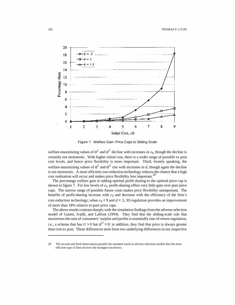
The percentage welfare gain in adding optimal profit sharing to the optimal price cap isshown in figure 7. For low levels of c0, profit-sharing offers very little gain over pure pricecaps. The narrow range of possible future costs makes price flexibility unimportant. Thebenefits of profit-sharing increase with c0 and decrease with the efficiency of the firm’s

cost-reduction technology; when c0 = 9 and d = .5, SS regulation provides an improvementof more than 18% relative to pure price caps.

The above results contrast sharply with the simulation findings from the adverse selectionmodel of Gasmi, Ivaldi, and Laffont (1994). They find that the sliding-scale rule thatmaximizes the sum of consumers’ surplus and profits is essentially rate-of-return regulation,

i.e., a scheme that has U > 0 but αU = 0; in addition, they find that price is always greaterthan cost ex post. These differences stem from two underlying differences in our respective

Figure 7. Welfare Gain: Price Caps to Sliding Scale

242 THOMAS P. LYON

28 The second and third observations parallel the standard result in adverse selection models that the mostefficient type of firm receives the strongest incentives.

models. First, Gasmi et al. redistribute shared profits to consumers via a lump-sum transferrather than a change in price, so profit-sharing has no allocative efficiency effects. Second,they impose ex post limited liability for even the least efficient firm, so loss-sharing is nevera possibility.

It is interesting to compare the qualitative nature of the simulated sharing rules with thesharing plans put into practice. Greenstein et al. (1995) summarize several recent surveysof state incentive regulation plans for telecommunications, many of which include profitsharing. The general pattern they report shows firms’ share of profits tends to fall as thelevel of profits rises; many schemes return all profits above a certain level to ratepayers. Thispattern runs counter to the welfare-maximizing policy identified by the simulation. Presum-ably the political pressures on regulators make it difficult to allow firms to keep a large shareof profits when profits are high.

A final case study is provided by the profit-sharing plan used by Medicare for psychiatrichospitals. Under the so-called TEFRA29 system implemented in 1982, if hospitals reducedtheir costs below a target level, they could keep 50% of gains up to a maximum of 5% of thetarget. If costs were above the target, however, the hospital had to cover 100% of the excess.

Thus, αU = .5 < αL = 1.0, a plan that runs counter to the above findings for optimal sliding-scale regulation. Interestingly, TEFRA was modified for 1992 implementation to incorpo-rate loss-sharing provisions symmetric with those for gain-sharing. While the simulationresults above suggest that loss-sharing probably should have been even more extensive thangain-sharing, the change represents a big step in the direction of efficiency.30

7. Conclusions

This paper has presented a formal model of sliding-scale regulation and its benefits relativeto rate-of-return regulation and price-cap regulation. While profit-sharing does not necessar-ily offer an improvement over rate-of-return regulation, some degree of profit- and loss-shar-ing outside a deadband improves social welfare relative to pure price-cap regulation.Simulation results show that a significant departure from pure price caps—that is, sharing asubstantial portion of profits with ratepayers—may be welfare-enhancing. Furthermore, itmay be desirable from a welfare perspective to allow the firm to retain a greater share ofgains than of losses, though political pressures may militate against such a policy. Simulationalso suggests that the additional welfare benefits of profit-sharing over pure price caps aregreatest when the firm’s initial cost is high and cost-reducing innovations are difficult toachieve.

While the results of this paper are fairly simple and intuitive, they were obtained undersome restrictive assumptions. I assumed a single-product firm in a static setting, with noexogenous shocks to costs or demand. In addition, the regulator was assumed to know thefirm’s underlying production technology, i.e., there was no adverse selection problem.Finally, I made no attempt to distinguish between capital costs and operating costs; sincemost sliding-scale schemes use the firm’s rate-of-return on capital, this distinction may be

A MODEL OF SLIDING-SCALE REGULATION 243

29 This system was created as part of the Tax Equity and Fiscal Responsibility Act of 1982, hence theacronym.

30 For a discussion and critique of the initial TEFRA rules, see Cromwell, Ellis, Harrow and McGuire (1991).

important. A full understanding of sliding-scale regulation will only be achieved byintegrating these considerations into the analysis.

Appendix

Proof of Lemma 1: (a) As noted above, under pure price caps, expected profits are

π__

(e,p0) = ∫ 0

c0(p0 − c)q(p0)dF(c e) − ψ(e). Then, by the envelope theorem,

dπ__

(e∗,p0)dp0

= ∫ 0

c0[q(p0) + (p0 − c)q′(p0)]dF(c e).

By assumption, no drastic cost reduction is possible, and pM(0) > p0. Thus, revenue

is increasing in p0, so q(p0) + p0q′(p0) > 0. Since − cq′(p0) > 0, expected profits are

increasing in p0. It is clear that if p0 > c0 then π__ > 0 and if p0 = 0 then π

__ < 0. Since

π__ is continuous in p0, there exists some p_ > 0 such that π

__(e∗,p_) = 0 and

π__

(e∗,p) < 0 for all p < p_.

(b) Totally differentiating (8) and rearranging terms yields

dedp0

=

− q′(p0) ∫ 0

c0Fe(c e)dc

q(p0)∫ 0

c0Fee(c e)dc − ψ′′(e)

< 0.

(12)

Q.E.D.

Proof of Proposition 1: Suppose the same initial price p0 holds under all regimes. Let

eRORR solve (7), and ePC solve (8). Note that (7) and (8) are identical except thatthe integral in (8) has a smaller lower limit of integration. Thus, the price-cap firm’s

expected profits at eRORR are increasing in e. Because Fee(c e) < 0,

ePC > eRORR. This is true a fortiori if the initial price under price caps is less than

that under RORR. It is apparent from (7) that eRORR > 0, but under cost-plus

regulation effort is eCP = 0. Thus eRORR > eCP. Expected costs are always decreas-ing in effort because Fe(c e) ≥ 0. Q.E.D.

Proof of Proposition 2: Under RORR,

dW__

dαUαU

= 0

= ∫ 0

cU

(pU − c)q′(pU)

[(p0 − c)q(p0) − U]

q(pU) + (pU − c)q′(pU)dF(c e)dc

+ ∂W

__

∂e

∂e

∂αUαU

= 0

.(13)

244 THOMAS P. LYON

Note that the integral term (the allocative effect ∂W__

⁄ ∂αU) is negative, while thesecond additive term (the incentive effect) is positive. Thus, in general the sign

of (13) is ambiguous. However, if U = 0, then pU = c, and the integral term is

exactly zero; welfare increases with αU. Since (13) is continuous in U, profit-sharing is welfare-increasing for small positive values of U as well. Q.E.D.

Proof of Proposition 3: Under pure price-cap regulation, ∂pL ⁄ ∂c = ∂pU ⁄ ∂c = 0, and∂S_

⁄ ∂e = 0. Straightforward calculations yield

dW__

dαLαL

= 1

= ∫ cL

c0(p0 − c)q(p0) − L

1 −

q(p0)q(p0) + (p0 − c)q′(p0)

dF(c e)dc < 0.

(14)

By the definition of cL, (p0 − c)q(p0) − L < 0 for c > cL; thus, the first term in

brackets within the integral is negative. Further, if L ≤ 0, then c > cL impliesp0 < c; thus, the second bracketed term within the integral is positive. The integral

as a whole is negative, so a small decrease in αL increases welfare.

Similarly,

dW__

dαUαU

= 1

= ∫ 0

cU

∂π∂pU +

∂S

∂pU ∂pU

∂αUdF(c e)

= ∫ 0

cU

(p

U − c)q′(pU) [(p0 − c)q(p0) − U]

q(pU) + (pU − c)q′(pU) dF(c e)dc < 0.

(15)

Since cU defines the cost level below which earnings exceed U, pU − c > 0 for all

c < cU. Thus, the first multiplicative term within the integral is positive. Demand

is downward-sloping, so the second term is negative. Since p0 < pM(0) by assump-tion, the denominator of the last term—which is equal to the marginal change inrevenue with an increase in price—is positive. Finally, (p0 − c)q(p0) − U > 0, andthe numerator of the last term is negative. Thus, the integral as a whole is negative,

and a small decrease in αU increases welfare. Since αL < 1, profits remain non-negative. Q.E.D.

Proof of Proposition 5: Differentiating welfare with respect to U yields

dW__

dUU = 0

= ∂W__

∂U +

∂W__

∂e

∂e

∂U + ∆

f(cU e)

∂cU

∂U + Fe(c

U e) ∂e

∂U

. (16)

The first additive term is negative, representing the loss of allocative efficiencycreated when a deadband makes price unresponsive to cost. The second additiveterm is positive due to the enhanced incentive for cost reduction provided by thedeadband. The third additive term is positive because a larger deadband generatesfewer costly rate reviews. Thus, if the first term is bounded, there exists some ∆

A MODEL OF SLIDING-SCALE REGULATION 245

large enough to make a deadband desirable. Suppressing the dependence of pU onc, straightforward calculation shows that

∂W__

∂U

U = 0

= (1 − αU) ∫ 0

p0 (pU − c)q′(pU)q(pU) + (pU − c)q′(pU)

dF(c e)dc

< maxc

(pU − c)q′(pU)

q(pU) + (pU − c)q′(pU).

(17)

The denominator of this last expression is positive, since pU is less than themonopoly price. Since q′(p) is finite, the numerator is bounded. Hence the size ofthe allocative effect is bounded, and there exists some ∆ large enough thatdW__

⁄ dU > 0 at U = 0. A similar argument can be made for L < 0. Q.E.D.

References

Armstrong, Mark, Simon Cowan, and John Vickers. 1994. Regulatory Reform: Economic Analysisand British Experience. Cambridge, MA: The MIT Press.

Banks, Jeffrey S. 1992. “Monopoly Pricing and Regulatory Oversight,” Journal of Economics andManagement Strategy 1: 203-233.

Braeutigam, Ronald R., and John C. Panzar. 1993. “Effects of the Change from Rate-of-Regulation toPrice-Cap Regulation.” American Economic Review 83: 191-198.

Braeutigam, Ronald R., and James P. Quirk. 1984. “Demand Uncertainty and the Regulated Firm.”International Economic Review 25: 45-60.

Cabral, Luis M. B., and Michael H. Riordan. 1989. “Incentives for Cost Reduction under Price CapRegulation,” Journal of Regulatory Economics 1: 93-102.

Clemenz, Gerhard. “Optimal Price Cap Regulation.” 1991. Journal of Industrial Economics 39:391-408.

California Public Utilities Commission. 1990. “Order Instituting Rulemaking on the Commission’sown motion to change the structure of gas utilities’ procurement practices and to propose refine-ments to the regulatory framework for gas utilities,” R.90-02-008.

Cromwell, Jerry, Randall P. Ellis, Brooke Harrow, and Thomas P. McGuire. 1991. “A ModifiedTEFRA System for Medicare Discharges from Psychiatric Facilities.” Mimeo, Boston University.

Fitzpatrick, Mary. 1987. “A Test of Passive Regulation using an Endogenous Switching Regression.”Discussion Paper EAG 87-5, U.S. Department of Justice, Antitrust Division, Economic AnalysisGroup.

Gasmi, F., M. Ivaldi, and J.J. Laffont. 1994. “Rent Extraction and Incentives for Efficiency in RecentRegulatory Proposals.” Journal of Regulatory Economics 6: 151-176.

Greenstein, Shane, Susan McMaster, and Pablo T. Spiller. 1995. “The Effect of Incentive Regulationon Infrastructure Modernization: Local Exchange Companies’ Deployment of Digital Technol-ogy.” Journal of Economics and Management Strategy 4: 187-236.

Indiana Utility Regulatory Commission. 1990. Petition of Public Service Company of Indiana, Inc.,for the Approval of Permanent Rates.... Cause No. 37414-S2.

Joskow, Paul. 1974. “Inflation and Environmental Concern: Structural Change in the Process of PublicUtility Regulation.” Journal of Law and Economics 17: 291-327.

Joskow, Paul, and Richard Schmalensee. 1986. “Incentive Regulation for Electric Utilities.” YaleJournal on Regulation 4:1-50.

Kahn, Alfred E. 1989. The Economics of Regulation. Cambridge, MA: The MIT Press.Laffont, Jean-Jacques, and Jean Tirole. 1993. A Theory of Incentives in Procurement and Regulation.

246 THOMAS P. LYON

Cambridge, MA: The MIT Press.Lyon, Thomas P. 1995. “Regulatory Hindsight Review and Innovation by Electric Utilities.” Journal

of Regulatory Economics 7: 233-254.Lyon, Thomas P., and Haizhou Huang. Forthcoming. “Innovation and Imitation in an Asymmetrically-

Regulated Industry.” International Journal of Industrial Organization.Majumdar, Sumit K. 1995. “Regulation and Productive Efficiency: Evidence from the U.S. Telecom-

munications Industry.” Working Paper 9504-14, School of Business Administration, University ofMichigan.

Milgrom, Paul, and Chris Shannon. 1994. “Monotone Comparative Statics.” Econometrica 62:157-180.

Peltzman, Sam. 1976. “Toward a More General Theory of Regulation.” Journal of Law and Economics19: 211-248.

Pint, Ellen M. 1992. “Price-Cap versus Rate-of- Return Regulation in a Stochastic-Cost Model.” TheRAND Journal of Economics 23: 564-578.

Rogerson, William P. 1985. “The First-Order Approach to Principal-Agent Problems.” Econometrica53: 1357-1367.

Sappington, David E. M., and David S. Sibley. 1992. “Strategic Nonlinear Pricing under Price-CapRegulation.” The RAND Journal of Economics 23: 1-19.

Sappington, David E.M., and Dennis L. Weisman. Forthcoming. Designing Incentive Regulation forthe Telecommunications Industry, Cambridge, MA: The MIT Press.

Schmalensee, Richard. 1989. “Good Regulatory Regimes.” The RAND Journal of Economics 20:417-436.

Stefos, Theodore, Nicole Lavallee, and Frank Holden. 1992. “Fairness in Prospective Payment: AClustering Approach.” Health Services Research 27: 239-261.

Weisman, Dennis L. 1993. “Superior Regulatory Regimes in Theory and Practice.” Journal ofRegulatory Economics 5: 355-366.

A MODEL OF SLIDING-SCALE REGULATION 247