A Model of Mental Budgeting: Consumer Theory and ...

A Model of Mental Budgeting: Consumer Theory and Inaccurate

Choice

Rafael Nunes Teixeira∗

July 8, 2016

Abstract: Commonly, Economic Theory assumes that money is fungible. However, evidence from Behavioral Economics

(Thaler (1999), Shapiro and Hastings (2013)) indicates this assumption may fail in many behaviors. One possible explanation

for this failure is the use of Mental Budgets, which indicates that people classify their money into expenditure categories. In

this work, it is developed a theoretical model that captures the idea of Mental Budgeting and discuss the consequences of such

assumption for the Consumer Theory. In addition, we highlight some behavioral observations of such agent. This creates new

interpretations for some anomalies such as the Preference Reversal.

Key words: Consumer Theory, Mental Budgeting, Mental Accounting

1 Introduction and Background:

One of the most important topics for Behavioral Economics is Mental Accounting. As Thaler (1999) described:

“Mental accounting is the set of cognitive operations used by individuals and households to organize, evaluate, and keep track

of financial activities.” (Thaler (1999), p.183). These cognitive operations are observed through many different behaviors

which often shows that people do not treat money as a fungible asset. That is, people behave as if money is not mutually

interchangeable to every and any situation.

One theoretical development of Mental Accounting is the idea of Mental Budgeting. This idea points that people classify

their money into expenditure accounts and then buy respecting the restrictions imposed by each of these account. Thaler (1999)

argued that: “Both the sources and uses of funds are labeled in real as well as in mental accounting systems. Expenditures are

grouped into categories (housing, food, etc.) and spending is sometimes constrained by implicit or explicit budgets.” (Thaler

(1999), p.183).

Mental Budgeting was first proposed by Thaler (1985) and later Heath and Soll (1996)s empirical analysis enhanced the

idea. Hearth and Soll selected a group of MBA students who displayed predetermined weekly or monthly budgets for food,

entertainment and clothes. Then, they simulated different situations and analyzed the hypothetical choices made by these

subjects. The analysis showed that gaining or losing objects and amounts of money that are associated with one category∗Mestre em Economia pela Unb. Cotato: [email protected]

1

(e.g. entertainment) led to great consumption’s changes for objects within the same category (e.g. entertainment), but it did

not lead to consumption’s changes for products within others categories (e.g. clothes). The Traditional Economical theory

usually explains this choice pattern using Income Effects or Satiation Effects (decreasing marginal utility). However, the study

indicates that these choices observed by Heath and Soll (1996) contradict these explanations 1 and, in this sense, they strongly

support the idea that consumers use multiple budgets.

The empirical research analyzing this sort of behavior grew during the last decade and created more evidences suggesting

people might use Mental Budgeting. Antonides, de Groot and van Raaij (2011) found that the Dutch population widely

uses Mental Budgeting in their day-life decisions and investigated which personal characteristics could be related to its use.

Fennema and Perkins (2008) described how proper training could diminish some uses of Mental Budgeting. Shapiro and

Hastings (2013) analyzed real consumption of gasoline and their results “consistently reject the null hypothesis that households

treat gas money as fungible with other income”(Shapiro and Hastings (2013), p.1449). Shapiro and Hastings perceived that

increases on the gasoline’s price systematically led the individuals to decrease the “quality” of the gas that they consume.

They compared these changes caused by price variations with changes caused by income variations and concluded that the

data could not be explained by Income Effects. Moreover, their results indicate that a model adapting Mental Budgeting

displays the best possible fit for their data.

Although there are several empirical studies supporting the idea that people behave as if they are using the process de-

scribed by Mental Budgeting, theoretical models incorporating this idea are almost absent in the literature. Some studies

tried to incorporate Mental Budgeting but often focusing on other aspects of people’s choices (e.g. preference). For example,

Thaler (1985) proposes a model with Transaction Utility and multiple budgets, but the author does not describe many theoret-

ical consequences 2of assuming multiple budgets. In a similar way, David Just (2013) presents a model with multiple budgets

and reference based utility, but also focuses on the utility and does not discuss many consequences of classifying money into

categories.

We develop a theoretical model that captures the general idea described in Mental Budgeting and thoroughly investigates

its consequences in the Consumer Theory. By developing a formal model for Mental Budgeting, we are able to understand the

theoretical and the empirical implications that can be used to verify whether Mental Budgeting is appropriate. Besides that, a

formal model can lead to new intuitions about the behavior of people who perceive money as non-fungible.

The proposed model differs from the traditional consumer problem by how the agent formulates his budget constraint.

Also, it describes the idea of Mental Budgeting in a very similar way to what is presented in Thaler (1985) and Just (2013), but

it differs from those papers because of its careful formalization and due to the fact that it maintains the traditional preferences

(i.e. Transitive, Complete and “Independent from the Context”). Usually, most of the anomalies described in Behavioral1Hearth and Soll(1996) gave the following example to show how these violations may occur:

Event 1: You spent 50$ on a ticket sport (entertainment category):(Question 1) Would you purchase a $25 theater ticker later in the week? “No.”Event 2: You are given the ticket above (entertainment category):(Question 2)Would you purchase a $25 theater ticker later in the week? “Yes.”Event 3: You hear of a flu epidemic on the news. You spend $50 for an inoculation.(Question 3)Would you purchase a $25 theater ticker later in the week? “Yes.”The pattern found in the questions 1 and 2 could be explained by Income Effects, but reduces the impact of Satiation Effects. The pattern in questions 1

and 3 could be explained by Satiation Effects, but reduces the impact of Income Effects. Several questions similar to these ones were ask and the patternfound was alike the answers described above. For more information, Hearth and Soll(1996).

2Thaler (1985) describes many practical consequences of assuming multiple budgets.

2

Economics are associated with an inconsistency in the preference ordering. Since we assume the standard preferences, we

are able to observe the implications solely resulting from Mental Budgeting. This is a new way to proceed and it creates a

new interpretation for some described anomalies (e.g. Preference Reversal). In order to identify the anomalies associated with

this new interpretation, the term Inaccurate Choice will be defined in Section 5. As we will point, this distinction between

an inconsistency caused by the preference ordering and an inconsistency caused by the perception of the constraints can be

fundamental for better experimental designs.

The next section describes the model’s general setup. The third section describes the agent with Mental Budgeting in the

Consumer Theory. In the fourth section, we show the general consequences of considering this kind of agent in the Consumer

Theory. The fifth section analyzes behaviors associated with this agent and defines the idea of Inaccurate Choice by contrasting

it with a Preference Reversal. In the sixth section, we discuss further modifications for the proposed setup. In the last section,

there is a general conclusion.

2 Setup for Mental Budgeting:

Consider the a Consumption Set X = Rn+, a vector x ∈X represents a consumption bundle and xi is the i− coordinate

of the vector x. The consumer has a preference relation %⊆ X ×X . We will consider through the text the following axioms

over %:

A1-Complete: For all x and y ∈ X , either x % y or y % x.

A2-Transitive: For any x,y and z ∈ X , if x % y and y % x =⇒ x % z.

A3-Continuous: For any sequence {(xn,yn)}∞n=1 with xn % yn for all n, x = limn→∞xn and y = limn→∞yn =⇒ x % y.

When necessary, the following axioms will be used:

A4-Locally Non-Satiable: For every x ∈ X and every ε > 0, there is y ∈ X such that ||y−x||< ε and y ≻ x.

A5-Strongly Monotone: For every x,y ∈X , if xi > yi∀i =⇒ x ≻ y

Assuming A1, A2 and A3, the preference relation, %, can be represented by a continuous utility function U : X → R

(Debreu (1954) ).

In the traditional model, given a price, p ∈ Rn++, and a wealth, w ∈ R+, a Budget Set, B(p,w) = {x|x ∈ X ,∑n

i=1 xi pi≤w},

is defined to describe the consumer’s budget constraint. Differently, an agent with Mental Budgeting has to classify the money

into categories and each category has to be identified by which objects it has. We define that the agent has an Expenditure

Categorization identifying the Expenditure Category for each object and an Allocation Rule identifying the Mental Allo-

3

cations that represent the quantities of money for each category.

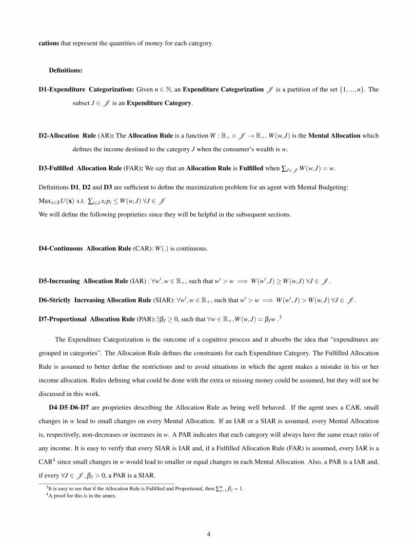
Definitions:

D1-Expenditure Categorization: Given n ∈ N, an Expenditure Categorization J is a partition of the set {1, ...,n}. The

subset J ∈ J is an Expenditure Category.

D2-Allocation Rule (AR): The Allocation Rule is a function W : R+×J → R+. W (w,J) is the Mental Allocation which

defines the income destined to the category J when the consumer’s wealth is w.

D3-Fulfilled Allocation Rule (FAR): We say that an Allocation Rule is Fulfilled when ∑J∈J W (w,J) = w.

Definitions D1, D2 and D3 are sufficient to define the maximization problem for an agent with Mental Budgeting:

Maxx∈XU(x) s.t. ∑i∈J xi pi ≤W (w,J) ∀J ∈ J

We will define the following proprieties since they will be helpful in the subsequent sections.

D4-Continuous Allocation Rule (CAR): W (.) is continuous.

D5-Increasing Allocation Rule (IAR) : ∀w′,w ∈ R+, such that w′ > w =⇒ W (w′,J)≥W (w,J) ∀J ∈ J .

D6-Strictly Increasing Allocation Rule (SIAR): ∀w′,w ∈ R+, such that w′ > w =⇒ W (w′,J)>W (w,J) ∀J ∈ J .

D7-Proportional Allocation Rule (PAR):∃βJ ≥ 0, such that ∀w ∈ R+,W (w,J) = βJw .3

The Expenditure Categorization is the outcome of a cognitive process and it absorbs the idea that “expenditures are

grouped in categories”. The Allocation Rule defines the constraints for each Expenditure Category. The Fulfilled Allocation

Rule is assumed to better define the restrictions and to avoid situations in which the agent makes a mistake in his or her

income allocation. Rules defining what could be done with the extra or missing money could be assumed, but they will not be

discussed in this work.

D4-D5-D6-D7 are proprieties describing the Allocation Rule as being well behaved. If the agent uses a CAR, small

changes in w lead to small changes on every Mental Allocation. If an IAR or a SIAR is assumed, every Mental Allocation

is, respectively, non-decreases or increases in w. A PAR indicates that each category will always have the same exact ratio of

any income. It is easy to verify that every SIAR is IAR and, if a Fulfilled Allocation Rule (FAR) is assumed, every IAR is a

CAR4 since small changes in w would lead to smaller or equal changes in each Mental Allocation. Also, a PAR is a IAR and,

if every ∀J ∈ J ,βJ > 0, a PAR is a SIAR.

3It is easy to see that if the Allocation Rule is Fulfilled and Proportional, then ∑mj=1 β j = 1.

4A proof for this is in the annex.

4

Putting the Expenditure Categorization in a behavioral perspective, if an object is not classified into any category, it would

be possible to observe this “no category” as a classification by itself5, being possible to represent this as a set for the partition.

To assume that the Expenditure Categorization is unambiguous, i.e. each object has one and only one category, might be

a strong presumption for an ex-ante moment. For example, studies of similarity (e.g. Tversky and Gati (1978) ) show that

an object might have many different classifications in a psychological perspective, and Cheema and Soman (2006) describe

ambiguities and changes on what could be seen as the object’s Expenditure Category. However, at the moment of the decision,

an object that is observed in more than one Expenditure Category would lead to indirect trade-offs between every object in

these categories, which might lead to these categories being behaviorally treated as one.

The Allocation Rule described here is useful to model behaviors that do not treat money as completely fungible. Although

there are many empirical evidences showing that people have different budgets for different expenditures, there is no evidence

indicating that the Allocation Rule is only related to the wealth, or that it can be defined by well behaved functions. Moreover,

there are many evidences showing (e.g., Milkman and Beshears (2009), Levav and McGraw (2009) ) that different sources

of money and frames might lead to different uses of the money. This implies that it is possible to have different values for

a Mental Allocation parting from the same wealth. Some of these situations are discussed in the sixth section, but it is not

incorporated in this work.

Even though there are other possible ways to describe an Allocation Rule and the Expenditure Categorization, the simple

assumptions described here and in the next section are enough to have a well defined Consumer’s Problem and to represent

a model similar to those in Thaler (1985) and Just (2013). Also, this framework describes the general idea of the Mental

Budgeting process and, by doing this, it identifies which could be adapted to incorporate other behaviors. This is also discussed

in the sixth section.

3 Mental Budgeting In the Consumer Theory: The Mental Budget Maximizer

(MBM)

The agent discussed in this work is named Mental Budget Maximizer (MBM). The MBM is an agent who has a

Continuous Utility Function, U : X → R, an Expenditure Categorization, J , and a Fulfilled Allocation Rule, W (.).

Therefore, given an MBM, a price vector,p ∈Rn++, and a wealth,w ∈ Rn

+, the Categorized Budget Set is the defined by:

CB(p,w) = {x|x ∈ X ,∑i∈Jxi pi≤W (w,J)∀J ∈ J }

An MBM consumer’s problem is:

Maxx∈XU(x) s.t. ∑i∈J

xi pi ≤W (w,J)∀J ∈ J (1)

Since J is a partition of X , the goods and services the individual consume, each i ∈ {1, ...,n} is part of a single Expen-

5At least, all unclassified objects treated equally (in an expenditure comparative situation) would form a category by themselves.

5

diture Category and there is no ambiguities on the restrictions. Thus, the Categorized Budget Set defines a Compact Set and,

since U(.) is a continuous function, there is always a solution for this problem.

Assuming the necessary and sufficient conditions to use the Lagrange Method:

L (x,λ ,µ) =U(x)−∑J∈J λJ(∑i∈J

xi pi −W (w,J)+n

∑i=1

µixi

The first order conditions are:

δL (x,λ ,µ)/δxi = δU(x)/δxi −λJ pi +µi; ∀i ∈ J

If (x∗,λ ∗) is the solution of the Lagrangian such that x∗a,x∗b,λJ > 0 are coordinates of x∗ and λ ∗, and a,b ∈ J:

δU(x∗)/δx∗a = λJ pa and δU(x∗)/δx∗b = λJ pb

δU(x∗)/δx∗a/δU(x∗)/δx∗b = pb/pa , ∀a and b ∈ J

Observe the Example 1 below that illustrates an MBM:

Example 1 - (Ana’s Problem)

Ana has the utility function U(.) = x0.8y0.2 + z+ 12 t, in which x represents food, y drinking, z nightclub and t theater. Ana

categorizes two types of expenditures, eating F = {x,y} and entertainment E = {z, t}. Her total wealth is w = 50, her Alloca-

tion Rule is such that she allocates 20$ for entertainment and 30$ for eating. The price are px = 2, py = 1, pz = 1,pt = 0.6.

The utility maximization problem for Ana is:

Maxx,y,z,t∈R+x0.8y0.2 + z+ 12 t

s.t 2x+ y ≤ 30

z+0.6t ≤ 20

The optimal choice of Ana is x∗ = 12,y∗ = 6,z∗ = 20, t∗ = 0.

This categorization reduces Ana’s utility level. If Ana had just one budget, her utility would be 50. In this situation Ana’s

utility level is almost 30. However, she is choosing her optimal bundle. That is, an agent with Mental Budgeting perceives a

different set of feasible bundles (CB instead of B) but, given this set of feasible bundles, the agent chooses the best option.

One should notice that Ana would spend all her money going to the nightclub if money were treated in the regular

way. In the MBM’s situation, the objects are not competing for the same resource, leading her to consume other goods too.

This example illustrates an important hypothetical aspect of Mental Budgeting (Thaler (1990), Shefrin and Thaler (1992)

6

): “Self-Control”6. The Expenditure Categorization and the Allocation Rule create a self commitment with some kinds of

consumption7. This is one behavior associated with this setup. Before exploring other behaviors related to it, we shall

investigate its theoretical consequences.

4 Consequences on the Consumer Theory:

How does the traditional Consumer Theory change if we allow an MBM agent? In this section we will define the

Demand Correspondence, Indirect Utility and Expenditure Minimization Problem for an MBM and we will discuss in which

circumstances it is possible to preserve some proprieties obtained for the traditional consumer in each of those problems.

The proofs of the results are in the annex.

4.1 Implications on the Demand Correspondence

The (Walrasian) Demand Correspondence, D : Rn++ ×Rn

+ ⇒ Rn+, D(p,w) ⇒ x , is the rule that characterizes the

optimal consumption vectors for each price vector, p ∈Rn++, and wealth, w ∈ R+. Since the Weierstrass Theorem guarantees

the existence of a maximum for MBM’s consumer problem, see Equation 1, the Demand Correspondence, D(p,w), is always

well defined.

In the usual consumer problem, if we assume that U(.) is continuous and representing a Locally Non-Satiable Preference,

the Demand Correspondence satisfies the properties bellow. After each property, we discuss under which conditions they are

still valid for the MBM’s Demand Correspondence:

1. Homogeneity of degree zero in (p,w). The Demand Correspondence of an MBM with a PAR satisfies this property.

2. Walras’s Law: p×x = w ∀D(p,w). The Demand Correspondence of an MBM with a Strongly Monotone Preference8

satisfies this property.

3. If % is convex (such that U(.) is quasi-concave) then D(p,w) is a convex set. If %is strictly convex (such that U(.) is

strictly quasi-concave) then D(p,w) consists of a single element. The convexity and uniqueness of D(p,w) under these

conditions are still valid for the MBM’s Demand Correspondence.

A PAR is a strong assumption for the Allocation Rule but it is required for maintain the homogeneity of degree zero of

the Demand Correspondence. Further discussion about this takes place in the section 4.2.

Given any Fulfilled Allocation Rule, Walras’s Law is satisfied if a Strongly Monotone Preference8 is assumed. If Walras’s

Law is not satisfied, the Allocation Rule is giving too much money for the Mental Allocation of an Expenditure Category in

which its objects has a Satiation Interval, i.e. an increase of consumption in this category will not improve the utility, but there

6At the same time, the setup may lead to strange behaviors once it can allocate all her money to one single object that might be the “opposite of self-control”.

7Similar to a person who has Petit Gateau as his favorite food but chooses to eat a steak in a restaurant because it is lunch and Petit Gateau is not afood lunch. An agent that behaves like this might not have money allocated for dessert. Other possibility is that he is choosing between different categories(Furtado, Nascimento and Riella (2015) ).

8It is possible to weaken this assumption. For example, assuming that for each J ∈ J there is an object i that for any x ∈ X the increase of any i wouldlead to an increase of the utility. Other possibility is a preference that is “locally non-satiable” in each category.

7

is still money left to be used in objects of this category. See Example 2 below:

Example 2 - (Walras’s Law)

Suppose an agent that consumes only two goods, x and y, and with the utility function: U = Min{x,y}. The prices of x and

y are px = py = 1. The Expenditure Categorization of the agent divides X = {x,y} into J = {x} and K = {y}. The Allocation

Rule is such that W (w,J) = w ∀w ∈ [0,1) , W (w,J) = 1 ∀w ≥ 1 and W (w,K) = 0 ∀w ∈ [0,1) , W (w,K) = w−1 ∀w ≥ 1.

If w = 0.5, W (w,J) = 0.5 and w(w,K) = 0. Thus, the optimal bundles are any from [0,0] to [0.5,0].

In the example, the Allocation Rule is just giving money to be spend in x, but to consume it does not lead to an increase in

the utility. Thus, it is not necessarily optimal to completely spend the money.

It is possible to redefine the Allocation Rules in order to describe an end for this extra money. For example, this extra

money could be described as a different source for savings. Another possibility is reallocating the extra money for particular

categories, similar to what could happen to windfalls. Experimental evidence (e.g. Milkman and Beshears (2009) ) describe

that windfalls have high propensity to be spent in particular classes of objects (i.e. “frivolous” spending).

4.2 Implications on the Indirect Utility Function

The Indirect Utility Function describes the maximum utility level that can be reached given a price vector, p ∈Rn++,

and a wealth, w ∈ R+. For the MBM, v : Rn+×R+ ⇒ R is defined by:

v(p,w) : Maxx∈XU(x) s.t. ∑i∈J

xi pi ≤W (w,J)∀J ∈ J (2)

In the usual consumer problem, if we assume that U(.) is continuous and representing a Locally Non-Satiable Preference,

the Indirect Utility Function satisfies the properties bellow. After each property, we discuss under which conditions they are

still valid for the MBM’s Indirect Utility:

1. Homogeneous of degree zero in (p,w). The Indirect Utility of an MBM with a PAR satisfies this property.

2. Continuous on (p,w). The Indirect Utility of an MBM with a CAR satisfies this property.

3. Strictly increasing in w. Indirect Utility of two different MBMs would satisfy this property: an MBM with a Locally

Non-Satiable Preference and a SIAR or an MBM with Strongly Monotone Preference and an IAR.

4. Decreasing in p. No extra requirements necessary.

5. Quasiconvex in (p,w). The Indirect Utility of an MBM does not necessarily satisfy this property even if a PAR is

assumed.

8

The non-homogeneity of degree zero of the Indirect Utility of an MBM that does not have a PAR leads to interesting

implications. The MBM’s utility can even rise when p and w change by the same proportion (in some situations, even if w

increases less than p). This can be related to Money Illusion (see Shafir, Diamond, Tversky (1997) for an interesting dis-

cussion of this topic). This illusion describes the tendency of agents to prefer a situation where there is a wage increase (in

this setup, wealth) accompanied by an even bigger increase in the price level, instead of a situation without any change, e.g.

v(1.07w,1.1p)> v(w,p). See Example 3 below:

Example 3 - (Homogeneity of Degree zero)

Suppose an agent that consumes only two goods, x and y, and with the utility function U = x+2y. The prices of x and y

are px = py = 1. The agent’s Expenditure Categorization divides X into J = {x} and K = {y}. The Allocation Rule is such

that W (w,J) = w ∀w ∈ [0,1), W (w,J) = 1 ∀w ≥ 1 and W (w,K) = 0 ∀w ∈ [0,1) , W (w,K) = w−1 ∀w ≥ 1.

If w = 1. Any λ ≤ 1 will describe v(λp,λw) = v(p,w). Any λ > 1 will describe v(λ p,λw)> v(p,w).

An Allocation Rule might start assigning more money for categories of which the consumption of its objects leads to a

smaller utility increase if compared to the consumption of price equivalent objects within others categories. With the increase

of wealth, the Allocation Rule might assign money to these other categories, making an increase of income and the price

level to be desirable. These situations may exemplify the Money Illusion as illustrated in the Example 3: Comparing similar

quantities9, y is preferred to x. A wealth increase leads to bigger proportional allocation for y, and even if a bigger price

increase happens, the utility level can rise.

The continuity of v(p,w) for an MBM that uses a CAR shows that little is required to obtain a well-behaved Indirect

Utility. However, a CAR does not guarantee that the Indirect Utility is increasing in w. See Example 4 below:

Example 4 - (Strictly Increasing in w)

Suppose an agent that consumes only two goods, x and y, and with the utility function: U = x0.99y0.1 . The prices of x and

y are px = py = 1. The Expenditure Categorization divides X into J = {x} and K = {y}. The Allocation Rule is such that

W (w,J) = w/2 ∀w ∈ [0,2) , W (w,J) = 2/w ∀w ≥ 2 and W (w,K) = w/2 ∀w ∈ [0,2) , W (w,K) = (w− (2/w) ∀w ≥ 2.

In this example, the Allocation Rule is such that an increase of w, when w > 2, will lead to an increase of consumption for

y but a decrease for x. Since the marginal utility of x is higher than the marginal utility of y, this change leads to a decrease of

the utility level. Moreover, the optimal bundle when w = 2 is not feasible for any w = 2, so the biggest utility level reached is

when w = 2, i.e. v(p,2)> v(p,w) ∀w = 2.

Even when the MBM uses an IAR, the Indirect Utility might have Satiation Intervals. That is, intervals in which changes

9The prices are the same.

9

on w or p do not imply in changes in the utility. In Example 2, for any 0 ≤ w ≤ 1 the maximum utility level is 0. Only when

w > 1, there is an increase of utility.

The third property describes the situations in which v(p,w) is strictly increasing in w and it shows in which situations the

MBM will not have a Satiation Interval. However, one should notice that the Walras’s Law is not necessarily satisfied if it is

assumed a Locally Non-Satiable Preference and a SIAR.

The fifth property shows that the Indirect Utility is not necessarily quasiconvex for any Allocation Rule described in

section 2. This demonstrates that in many cases the pattern of choice associated with an MBM agent does not follow the

same regularities of an agent who does not use Mental Budgeting. In this sense, this pattern can not be represented by an

adapted preference that is still transitive, complete, continuous and price independent. The Allocation Rule changes the set of

feasible bundles for each different price and wealth and defines a pattern of choice that is directly dependent on these factors.

However, in a situation outside the market (directly comparing bundles, without the use of prices and wealth), the MBM agent

would have a well defined preference. e.g. See Exemple 4: With prices px = 0.5, py = 0.5 and wealth w = 2, the agent would

consume (2,2). By changing the prices to p′x = 1 and p

′y = 1, and wealth to w

′= 4, the agent would consume (1,3). But, if it

is asked separately which of these two bundles the agent would prefer, the agent would strictly prefer (1,3) instead of (2,2).

Hence, with different prices and wealth, different choices are observed.

4.3 Implications on the Expenditure Minimization Problem

The MBM’s Expenditure Minimization Problem finds the minimal amount of money that is necessary to buy a bundle

which reaches a predetermined utility level and still satisfies the restrictions imposed by the Allocation Rule. The function

usually is defined by e : Rn++ ×U → Rn

+ where U ⊆ R is the set defined by the utility levels bigger than U(0) that U(.)

can reach, i.e. U := {u|u = U(x)∀x ∈ Rn+,U ≥ U(0)}. For the MBM, we need to address issues that do not appear in the

traditional Expenditure Minimization.

First, w is not necessarily equal to ∑ni=1 pixi since the Walras’s Law is not always satisfied. Observe the following example:

Example 5 - (Walras’s Law and Utility Upper Bound)

Suppose an agent that consumes only two goods, x and y, and with the utility function: U = x− y. The prices of x and

y are px = py = 1. The Expenditure Categorization divides X into J = {x} and K = {y}. The Allocation Rule is such that

W (w,J) = w/2 ∀w ∈ [0,2), W (w,J) = 1 ∀w ≥ 2 and W (w,K) = w/2 ∀w ∈ [0,1), W (w,K) = w−1 ∀w ≥ 2.

We want to define the Expenditure Minimization Problem in such a way that it would describe the example above as

e(p,1) = 2, but ∑ni=1 pixi = 1. For this instance, we assume that the agent might allocate resources in the form of d ∈ R+. d

is used to illustrate the amount of money the agent will not spend due to an err in the allocation (as described in the second

propriety of section 4.1). In this sense, d incorporates the difference between w and ∑ni=1 pixi. See the Equation 3 below for

a better understanding.

10

Additionally, there are utility levels that the agent can never reach due to their mental restrictions. In Example 5, the

utility level which this agent can reach is limited to 1, hence e(p,u) will not have a solution for any u > 1. Hence, we define

the Expenditure Minimization Problem in the region where it always has a solution to avoid this type of situation. So, given a

price vector p∗ ∈ Rn++, define u := Sup{v(p∗,w)∀w ∈ R+} where v(p∗,w) is the MBM’s Indirect Utility. We will change U

into U ′(p∗) := {u ∈ R|U(0)≤ u < u}. Thus, the MBM’s Expenditure Minimization will be defined as, e : Rn++×U ′ → R+:

e(p,u) : Minx∈X ,d∈R+d +n

∑i=1

pixi s.t U(x)≥ u (3)

∑i∈J

xi pi ≤W (d +n

∑i=1

pixi,J)∀J ∈ J

In the usual consumer problem, if we assume that U(.) is continuous and representing a Locally Non-Satiable Preference,

the Expenditure Minimization satisfies the properties bellow. After each property, we discuss under which conditions they are

still valid for the MBM’s Expenditure Minimization

1. Zero when u takes on the lowest level of utility, No extra requirements necessary.

2. Homogeneous of degree 1 in p. The Expenditure Minimization of an MBM with a PAR satisfies this property.

3. Continuous on (p,u). The Expenditure Minimization of two different MBMs would satisfy this property: an MBM

with a Locally Non-Satiable Preference and a SIAR or an MBM with Strongly Monotone Preference and an IAR.

4. For all p∈Rn++, strictly increasing in u. The Expenditure Minimization of an MBM with a CAR satisfies this property.

5. Increasing in p. The Expenditure Minimization of an MBM with an IAR satisfies this property.

6. Concave in p. The Expenditure Minimization of an MBM does not necessarily satisfy this property even if a PAR is

assumed.

There are not many comments to be made about proprieties one, two, five and six. We will highlight the relation between

the proprieties three and four and the Indirect Utility.

The continuity of the Expenditure Function is reached once assumed a Strongly Monotone Preference and an IAR or a Lo-

cally Non-Satiable Preference and a SIAR. These requirements are different from those necessary for reaching the continuity

of the Indirect Utility. See Example 2, the Allocation Rule is Increasing and e(p,0) = 0 but e(p,ε)> 1∀ε > 0. The Indirect

Utility is continuous but the Expenditure Minimization Problem of the same agent is not.

The Expenditure Minimization is strictly increasing in u once a CAR is assumed. One should notice that the assumptions

required by the Indirect Utility (proprieties two and three) and those required by the Expenditure Minimization Problem

(proprieties three and four) are symmetric. This is important to the dual relation between the Expenditure Minimization and

the Indirect Utility.

11

4.4 Duality

Usually if a consumer has a continuous and strictly increasing utility function then, given p ∈ Rn++,w ∈ R++and

u ∈ U , the following duality relation is valid: v(p,e(p,u)) = u and e(p,v(p,w)) = w. Under what conditions are these

relations satisfied in the MBMs Setup?

Assuming a CAR does not ensure that the MBM’s Indirect Utility Function is strictly increasing in w.Hence, it is possible

to have multiple values of wealth, wn, reaching the same utility level, v(p,w1) = v(p,w2) = u and w1 = w2. In these situations,

the Expenditure Minimization’s value would be the minimum between these different values of wealth, i.e. given a u, define

W := {wn ∈ R+|v(p,wn) = u} and we will have e(p,u) = min{W}. Hence, e(p,v(p,w)) is not necessarily w. Yet, we proved10

that a CAR guarantees that e(p,u) is strictly increasing in u and if (x∗,d∗) is the minimal argument of e(p,u), then U(x∗) = u.

This is enough to prove that v(p,e(p,u)) = u.

Only when the agent uses an IAR or SIAR and has, respectively, a Strongly Monotone or a Locally Non Satiable Pref-

erences, v(p,w) is strictly increasing in w. As we described in the Second Section, every SIAR is an IAR, and every IAR is

a CAR. So, when the Indirect Utility is strictly increasing in w, the Expenditure Minimization of the same agent is strictly

increasing in u.

Proposition: Let v(p,w) and e(p,u) be the Indirect Utility and Expenditure Minimization Function for some MBM with

Strongly Monotone Preference, an IAR and a continuous utility function. Then ∀p ∈Rn++,w ∈ R+ and u ∈ U ′, we have:

1)e(p,v(p,w)) = w,

2)v(p,e(p,u)) = u.

Proof:

(1) Fix (p,w). By definition e(p,v(p,w)) ≤ w. Suppose that e(p,u) < w where u = v(p,w). Since e(.) is continuous,

there is an ε > 0 such that e(p,u+ ε) < w. Define wε = e(p,u+ ε) and by definition v(p,wε) ≤ u+ ε . Since v(.) is strictly

increasing in w this is a contradiction: v(p,w) = u > v(p,wε) = u+ ε > u. Thus, e(p,v(p,w)) = w.

(2) Fix (p,u). By definition v(p,e(p,u))≥ u. Suppose that v(p,w)> u where e(p,u) =w. Since v(.) is continuous, there is

an ε > 0 such that v(p,w−ε)> u. Define uε = v(p,w−ε) and by definition e(p,ue)≤ w−ε . Since e(.) is strictly increasing

in u this is a contradiction: e(p,ue)> e(p,u) and e(p,uε)≤ w− ε < w = e(p,u). Thus, v(p,e(p,u)) = u.

5 MBM’s Behaviors

We already showed that an MBM agent might suffer from Money Illusion, have self-control problems and have a

“observed preference ordering” that is directly dependent from the prices and wealth. In this section we will discuss and define

the idea of Inaccurate Choices and argue how this concept might help in experimental procedures.

10Annex of the Section 4.3.

12

5.1 Preference Reversals and Inaccurate Choices

According to Kahenman and Ritov (1994): “A preference reversal is said to exist when two strategically equivalent

methods for probing the preference between objects yield conflicting results” (Kahneman and Ritov(1994) p.25).

Preference reversals are often associated with any violation to the normative axioms defining the preference. Lichtenstein

and Slovic (1971) and Grether and Plott (1979) were the first ones analyzing such behaviors. In these studies, by observing

experimental choices, they systematically found inconsistencies comparing the choices between pairs of lotteries with similar

expected value and these lotteries respective willingness to pay (WTP)11.These lottery pairs were composed by one with high

winning chance and other with a lower chance but bigger prize. They found that most of the subjects reported a bigger WTP

for the lottery with the lower probability, but chose the lottery with higher probability.

In economic theory, if option A is priced higher than option B,it is expected that A is preferable to B. that is, ifWT P(A)>

WT P(B) then it is expected A ≻ B. is, if W T P(A) > W T P(B) then it is expected A B. In the Preference Reversal showed by

Lichtenstein and Slovic (1971), the subjects reported WT P(B)>WT P(A), but strictly preferred A to B, A ≻ B. As Kahneman

and Ritov wrote, this pattern of choice is usually related to possible inconsistencies in the preference. In this sense, theoretical

models were developed trying to incorporate this kind of behavior by adapting the preference’s setup. For example, Graham

and Sugden (1982) suggested capturing this behavior considering non transitive preferences. Tversky, Sattath, Slovic (1988)

suggested using context dependent preferences.

In a different approach, Tversky, Slovic and Kahneman (1990) used an experiment setup to explain Preference Reversals

(for lotteries) using a notion of Overpricing for the lottery of higher risk. We have interpreted the overpricing of long shots as

an effect of scale compatibility: because the prices and the payoffs are expressed in the same units, payoffs are weighted more

heavily in pricing than in choice (Tversky, Slovic and Kahenman (1990), p. 214).

This explanation relies on difficulties to evaluate the objects in different contexts. One evaluation occurs in choice terms,

another in monetary terms. A model with Mental Budgeting, which incorporates an incomparability aspect for money, can

lead to situations that could be described as a Preference Reversals in a way similar to the idea described by Tversky, Slovic

and Kahneman (1990). Since each category of objects is compared on different notions of money, it is possible that in pref-

erence terms A ≻ B, but in monetary terms WT P(B) >WT P(A). Yet, differently from a Preference Reversal, this pattern of

choice for an MBM agent is not associated with his preference between objects, but with the fact that the MBM thinks money

in a non-fungible way. Observe Anas Example again:

Example 1 - (Ana’s Problem):

Maxx,y,z,t∈R+x0.8y0.2 + z+ 12 t

s.t 2x+ y ≤ 30

z+0.6t ≤ 20

Ana’s optimal choice is x∗ = 12,y∗ = 6,z∗ = 20, t∗ = 0, with:

11The Willingness to pay of an Object is defined as the amount of money that makes the agent indifferent between this money and the object.

13

δU(x∗)/δx = 0.8(60.2)/120.2 = 0.6964 , px = 2

δU(x∗)/δ z = 1, pz = 1

Ana would be in a better situation by trading all her units of x and y for more units of z. However, Ana is willing to pay

2$12 for an extra marginal unity of x but only 1$13 for an extra marginal unity of z, even though the marginal utility of z is

bigger than the marginal utility of x. This happens due to the fact that each amount of money is withdrawn from a different

account which are not directly comparable. Therefore, one observes 1$ ∼ a and x ∼ 2$, however, these monetary values are

not perceived as comparable.

The described behavior might be seen as a Preference Reversal, however there is no change on the preference between

objects. It is the fact that money is not being treated as fungible that leads to this situation. This pattern of choices is what we

define as an Inaccurate Choice, a situation with the same behavioral consequence as the Preference Reversal but caused by

the use of multiple budgets.

The MBM does not perceive money as fungible14, but the agent still chooses optimally. That is, the agent knows what

he or she wants but, due to the agent’s perception of money, it is defined a different set of feasible bundles. The division

of money into categories creates a different monetary comparison for each category and these monetary comparisons are

not necessarily the same described by the preference ordering. Thus, Inaccurate Choice is occurring due to the difference

between the monetary comparison and the preference ordering. i.e. In the presence of an Inaccurate Choice, the preference

is well determined, A ≻ B, but the multiplicity of the budgets constraints leads to different monetary comparison, WT P(B)>

WT P(A).

The Inaccurate Choice’s existence leads to important experimental implications. Many experiments observe the WTP

as a preference’s reflex and this might not be true for an agent who does not treat money as fungible. In this sense, the

experimental setup must control if the choices changes happen due to a change on the constraints perception or due to a

change on the preference ordering. For example, objects that are classified by the agent into different categories cannot have

their WTP directly compared.

5.2 Experimental Observations and Inaccurate Choices

How to identify a category?

Usually, in an experimental procedure, the category of an object is given by a predetermined categorization or by identify-

ing it with a self-reported perception for category or similarity between objects (Heath and Soll (1996), Cheema and Soman

(2006)). These methods can lead to interesting intuitions, but the object’s expenditure category is not necessarily equal to the

categorization’s outcome observed in these perspectives. Is it possible to identify the Expenditure Categorization by observing

a behavior?

If a consumed object within a category has its utility related to a consumed object within another category, a price change

12This values are per unity.13The agent would be willing to pay up to 1.2$ per unity.14There are evidences that also time is not treated as fungible as well (Rajagopal (2009)).

14

for any consumed object within any of these categories would lead to consumption changes in both categories. In the same

situation, a wealth change that alters the amount of money allocated for a category that has an object which has its utility

related to an object in another category would lead to consumption changes in both categories. In this sense, it is not easy

to differentiate the categories of each object by a simple analysis of wealth and price changes. However, as Heath and Soll

(1996) and Hastings and Shapiro (2014) have done, it is possible to obtain important observations by inspecting the income

and substitution effects for these changes.

An Inaccurate Choice is the more transparent way to detect the expenditure category for different objects. Two objects

must be compared in different monetary perspectives for an Inaccurate Choice to occurs and, hence, each object has to be in a

different category. At the same time, an Inaccurate Choice would never happen for two objects in the same category. So, for

an MBM, given objects A,B in X , if quantity of A, xA, is preferable to a quantity of B, xB, so xA ≻ xB and this person is willing

to pay more for xB than for xA, WT P(xA)<WT P(xB), A and B must be in different Categories.

It is possible to simulate an Inaccurate Choice in order to identify if two objects have the same category. For doing so,

compare quantities of A and B, xA and xB, and identify a quantity which they are indifferent, xA ∼ xB. If A and B are both

in the same category, it is expected that WT P(xA) ∼= WT P(xB). If WT P(xA) = WT P(xB), the objects are being evaluated in

different monetary perspectives and have different categories. For example, if a person has a category for expenditures with

food and another for expenditures with transportation, an experimental procedure might compare grams of sirloin with liters

of gas. A person can be indifferent between 20 liters of gas and 500 grams of sirloin, but this same person might be willing to

pay more for the 20 liters of gas. This procedure can be done for any object consumed to identify the category of any object.

As discussed in the second section, there are evidences that the category of objects might be context dependent. It is possi-

ble to observe these changes by simulating an Inaccurate Choices in different contexts and noticing within which category the

objects is classified. This might be fundamental to completely differentiate an Inaccurate Choice and a Preference Reversal.

For the change in the Willingness to Pay be considered part of an Inaccurate Choice, the preference can not alter with the

context of the choice. This means that in different contexts the quantities observed as indifferent have to maintain the same,

i.e. if there is a indifference between xA and xB in one context, we cannot find an indifference between xA and xB with xA = xB

in another context. Nevertheless, the realization of these procedures would give us more information about the Categorization

Process and help in the development of a better theory.

How to identify a Allocation Rule?

Given a Expenditure Categorization, the Allocation Rule can be identified by analyzing the amount of money spent in

each category for different values of wealth. In this sense, given a p ∈Rn++, we have ∑i∈J xi pi ≤W (w,J)∀J ∈ J , one should

change the wealth, w, and calculate the different Mental Allocations for each category, W (w,J) ∀J ∈ J . However, the fact

that the Walras’s Law might not be satisfied creates some difficulties in this procedure. Without the Walras’s Law, ∃J ∈ J

such that ∑i∈J xi pi <W (w,J) and ∑ni=1 xi pi < w, i.e. there is an amount of money in some categories that would not be spend.

15

In these situations, a price change would be necessary to properly identify the Mental Allocations15. A price increase for a

consumed object in the category associated with the extra money, as described in section 4.1, would lead to an increase in the

amount of money spent in this category without changing the spending in the others categories.

As discussed in the second section, there are evidences showing that different sources of wealth might lead to different

Mental Allocations. Besides that, the model proposed here identifies an Allocation Rule that is independent from the prices.

This procedure might elucidate these features and it gives a better understanding of the Allocation Rule.

6 Further Modifications in Modeling the MBM

The model here presented is a simple and formal configuration to capture the Mental Budgeting’s idea. By being

simple, it ignores some experimental evidence. By being formal, it gives a setup and a way to think about the necessary

modifications.

As experimental evidence show, the Expenditure Categorization might be context dependent (Cheema and Soman (2006)).

For example, changing the set of the available objects (Tversky and Gati (1978)) or creating situations in which there is an

emphasis in some aspects of the choice (Cheema and Soman (2006)) might change the object’s Expenditure Categorization.

Further research is needed in order to better understand the Expenditure Categorization process. A model that endogenizes the

Categorization Process might describe behaviors like “penny-a-day”(Gourville (1998)) as the following situation exemplifies:

”John starts his day in a local coffee place with a caffe latte grande and a newspaper. Together, he spends on coffee and

newspaper slightly over $3 a day. He then takes public transportation to get to work. One day Mary joins John for the morning

coffee, and he tells her that he dislikes public transportation, but that he cant afford to buy a car. Mary says that she has just

bought a small car, financed at $99 a month. John sighs and says that he knows that such financing is possible, but that he

cant even afford to spend an extra $99 a month. Mary replies that if he were to give up on the caffe latte and newspaper

each morning, he could buy the car. John decides to buy the car and give up on the morning treat.”(Gilboa,Postlewaite and

Shmeidler (2009) p.2) In this example, John might have a well defined preference between Cars and Breakfasts and he was

not perceiving that these objects were competing for the same resources. By being given a “new perspective”, he is able to

compare these objects in a resource perspective. This kind of behavior could be caused by a change in the object’s category.

Experiments about Mental Accounting, including Kahneman and Tversky (1981), describe that losing an object or losing

an equivalent amount of money lead to different behaviors. In both situations the total wealth are the same and the model

described would have to observe the same behavior in both situations. Other experimental evidences show that different

sources of money might lead to different behaviors (e.g., Milkman and Beshears (2009), Levav and McGrew (2009)). The

model ignores the source of the income as a variable defining the Mental Allocations. In this sense, the Allocation Rule might

be changed to consider this variables.

All phenomena described in this section are framing effects and related to a rupture of the invariance assumption, i.e.

“different representations of the same choice problem should yield the same preference” (Kahenman and Tversky (1986),

p.S253). That is, all the situations described here have the same set of objects, but peculiarities of the context lead to different

15Since it is possible that there are several categories which have money allocated that is not spent.

16

outcomes. In the same way that frame effects are being incorporated in the utility function, frame effects could be incorporated

in the (budget) constraints. The realization of the procedures described in Section 5.3 would give many insights about the

features described in this section and would help improve the theory.

7 Conclusion

The research about Mental Accounting started trying to answer a question “How do people think about money?”

(Thaler (2015) ). In the traditional Consumer Theory found in any Microeconomics’s textbook, money and preferences are

represented in different ways. Preferences are represented by the Utility Function and Axioms of Revealed Choice, while

money is represented by the Budget Constraint. Furthermore, the usual consumer has preferences that are independent from

the price vector. Experimental evidences (as described in Thaler (1999) ) might suggest that taking part of a deal might lead to

an “utility increase” and the way that the price is observed might change the object’s “utility”. However, the representation of

“how people think about money” in the Consumer Theory takes place mostly on the representation of the monetary constraint.

In this sense and using the evidence related to Mental Budgeting (Thaler (1999), Just (2013), Heath and Soll (1996) ), we

describe here a model that incorporates ideas associated with the notion that money is classified and not treated as fungible.

The proposed model leads to interesting observations on the Consumer Theory described in Sections 3 and 4. Homo-

geneity, continuity and other usual proprieties found in the consumer’s analyzes are only preserved if the way that money

is categorized follows some regularities. These observations may be used to test further implications and to construct better

theories, as discussed in Section 5. Also, the fact that the quasi-convexity of the Indirect Utility16 is not necessarily preserved

even if a PAR is assumed indicates that the MBM agent’s pattern of choice cannot be totally incorporated by a modified utility

function respecting the regular axioms (transitivity,completeness, continuity and price independent).

Furthermore, by analyzing the consequences of multiple budgets, in Section 5, it is described that some unusual observed

behaviors might be explained by the consumer’s incapacity to observe his budget constraint in a “holistic” way. We described

the concept of Inaccurate Choice to illustrate a decision similar to a Preference Reversal but that is caused by the perception

of the budget constraints, not due to an inconsistency on the preference ordering between objects.

The usual focus of behavioral economics is on the preferences formulation, leaving the the constraints’s perception aside.

If Mental Budgeting occurs as experimental evidences indicate (Thaler (1999), Heath and Soll (1996), Hastings and Shapiro

(2013) ), the experimental procedures must control the possibility that behavioral changes might happen due to the con-

straints’s perception, and be not directly related with the perference’s formulation. For example, the willingness to pay of

objects in different categories might not represent the preference ordering between these objects.

The model presented here tries to help on the understanding of the perception of the constraints. A better understanding

of this can be critical to the development of more accurate Economic Theory.

16Similar observation could be made by the concavity of the Expenditure Minimization.

17

Annex

Section 3’s Proofs:

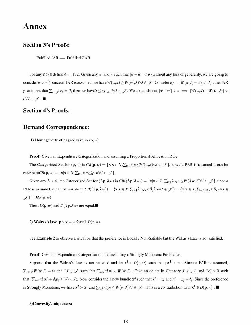
Fulfilled IAR =⇒ Fulfilled CAR

For any ε > 0 define δ := ε/2. Given any w′ and w such that |w−w′|< δ (without any loss of generality, we are going to

consider w>w′), since an IAR is assumed, we have W (w,J)≥W (w′,J)∀J ∈J . Consider eJ := |W (w,J)−W (w′,J)|, the FAR

guarantees that ∑J∈J eJ = δ , then we have0 ≤ eJ ≤ δ∀J ∈ J . We conclude that |w−w′|< δ =⇒ |W (w,J)−W (w′,J)|<

ε∀J ∈ J . �

Section 4’s Proofs:

Demand Correspondence:

1) Homogeneity of degree zero in (p,w)

Proof: Given an Expenditure Categorization and assuming a Proportional Allocation Rule,

The Categorized Set for (p,w) is CB(p,w) = {x|x ∈ X ,∑i∈Jxi pi≤W (w,J)∀J ∈ J }, since a PAR is assumed it can be

rewrite toCB(p,w) = {x|x ∈ X ,∑i∈Jxi pi≤β jw∀J ∈ J }.

Given any λ > 0, the Categorized Set for (λp,λw) is CB((λp,λw)) = {x|x ∈ X ,∑i∈Jλxi pi≤W (λw,J)∀J ∈ J } since a

PAR is assumed, it can be rewrite to CB((λp,λw)) = {x|x ∈ X ,∑i∈Jλxi pi≤β jλw∀J ∈ J } = {x|x ∈ X ,∑i∈Jxi pi≤β jw∀J ∈

J }= MB(p,w)

Thus, D(p,w) and D(λp,λw) are equal.�

2) Walras’s law: p×x = w for all D(p,w).

See Example 2 to observe a situation that the preference is Locally Non-Satiable but the Walras’s Law is not satisfied.

Proof: Given an Expenditure Categorization and assuming a Strongly Monotone Preference,

Suppose that the Walras’s Law is not satisfied and let x1 ∈ D(p,w) such that px1 < w. Since a FAR is assumed,

∑J∈J W (w,J) = w and ∃J ∈ J such that ∑i∈J x1i pi < W (w,J). Take an object in Category J, i ∈ J, and ∃δi > 0 such

that (∑i∈J x1i pi)+δi pi ≤W (w,J). Now consider the a new bundle x2 such that x2

i = x1i and x2

i = x1i +δi. Since the preference

is Strongly Monotone, we have x2 ≻ x1 and ∑i∈J x2i pi ≤W (w,J)∀J ∈ J . This is a contradiction with x1 ∈ D(p,w) . �

3)Convexity\uniqueness:

18

Proof:Given an Expenditure Categorization,

1)Get any x1 and x2 elements of D(p,w). Define x3 = αx1 +(1−α)x2 for any α ∈ [0,1]. U(x1) =U(x2) and px1 ≤ w,

px2 ≤w. We have ∑i∈J xni pi ≤W (w,J)∀J ∈J for n= {1,2}. Multiplying both sides by α to find α ∑i∈J xn

i pi ≤αW (w,J)∀J ∈

J , then α ∑i∈J x1i pi +(1−α)∑i∈J x2

i pi = ∑i∈J x3i pi≤ αW (w,J)+ (1−α)W (w,J) = W (w,J)∀J ∈ J . As U(.) is quasicon-

cave, U(x3)≥U(x1) =U(x2), since U(x1) is max of D(p,w) and x3 is affordable, we conclude that x3 is element of D(p,w).

2) Suppose by contradiction that D(p,w) does not consists in a single element and there are x1and x2 are elements of

D(p,w). Define x3 = αx1 +(1−α)x2, using a similar argument as above it is possible to show that ∑i∈J x3i pi ≤W (w,J)∀J ∈

J . As U(.) is strictly quasiconcave, U(x3)>U(x1) =U(x2), This would be contradiction with x1and x2 being maximums.

�

Indirect Utility Function:

1. Homogeneous of degree zero in (p,w)

Proof: Given an Expenditure Categorization and assuming a Proportional Allocation Rule:

The Indirect Utility of an MBM, given(p,w) is:

Maxx∈XU(x) s.t. ∑i∈J xi pi ≤ bJw∀J ∈ J

Consider λ > 0 and the Indirect Utility given (λp,λw):

Maxx∈XU(x) s.t. ∑i∈J xiλ pi ≤ bJλw∀J ∈ J

Which are the same problem. �

2. Continuous on p,w

Since U(x) is continuous, if Categorized Budget Set is defined by a continuous correspondence of compact values, the

Maximum Theorem would imply that v(p,w) is continuous on (p,w). We are going to prove that this is true for an MBM

using a CAR.

Proof: Given an Expenditure Categorization and assuming that a Continuous Allocation Rule, CB(p,w)= {x|x∈X ,∑i∈Jxi pi≤W (w,J)∀J ∈

J }, we will use wJ :=W (w,J) in order to simplify the notation.

To prove the correspondence’s upper hemicontinuity: Suppose (pm,wm)→ (p,w) and xm such that xm ∈CB(pm,wm)∀m.

Define p∗i := in f{pmi : m = 1, ...} and w∗

j := sup{W (wm,J)∀m}∀J ∈ J . p∗i ∈ R++∀i ∈ {1, ...,n} and w∗J ∈ R+ for each ∀J ∈

J . Define p∗as the vector of p∗i s and w∗as the vector of w∗Js. ∀m, CB(pm,wm)⊆CB∗(p∗,w∗) = {x|x ∈ X ,∑i∈Jxi p∗i ≤w∗

J∀J ∈

J }. CB∗ is a compact set, then there is a subsequence (xmk) of (xm) which xmk → x ∈CB(p∗,w∗). Since ∀k, ∑i∈J pmki xmk

i ≤

W (wmk ,J)∀J ∈ J when pmk → p, wmk → w and xmk → x, we have ∑i∈J pixi ≤W (w,J)∀J ∈ J . This concludes that CM is

19

defined by an upper hemicontinuous correspondence on (p,w).

To prove the correspondence’s lower hemicontinuity: Given (p,w) and a set I open which CB(p,w)∩ I = /0. Get x ∈

CB(p,w)∩ I, since I is open ∃λ ∈ (0,1) such that λx ∈ I. We have p.(λx) < w, moreover ∑i∈J λxi pi < wJ∀J ∈ J . Since

a CAR is assumed, ∀e > 0, there is a δ j such that |w−w′| < δ j =⇒ |W (w,J)−W (w′,J)| < e. Thus, ∃δ > 0 such that

for all (p, w) ∈ B((p, l),δ ), p(λx) < w and ∑i∈J λxi pi < W (w,J)∀J ∈ J . This concludes that CB is defined by a lower

hemicontinuous correspondence on (p,w).

We conclude that CB is defined by a continuous correspondence of compact values on (p,w) and, by the maximum theo-

rem, v(p,w) is continuous on (p,w).�

3. Strictly increasing in w

Proof 1 : Given an Expenditure Categorization and assuming an Increasing Allocation Rule and a Strongly Monotone

preference,

The Increasing Allocation Rule implies that if w′ > w then ∃J ∈ J such that W (w′,J) > W (w,J) and W (w′,K) ≥

W (w,K)∀K = J ∈ J .

Consider x∗ as the argmax of v(p,w). Given w′> w, ∃x′

such that x′i = x∗i ∀i ∈ K = J ∈ J , x∗

′i > x∗i ∀i ∈ J and such that

∑i∈Jx′i pi≤W (w,J)∀J ∈ J . The preference is Strongly Monotone, thus x′ ≻ x and it is affordable in v(p,w′). We conclude

that v(p,w′)≥U(x′)>U(x) = v(p,w) and the Indirect Utility is Strictly Increasing in w. �

Proof 2:Given an Expenditure Categorization and assuming a Strictly Increasing Allocation Rule and a Locally Non-

Satiable preference,

The Strictly Increasing Allocation rule implies that if w′ > w then W (w′,J)>W (w,J)∀J ∈ J .

Consider x∗ as the argmax of v(p,w). Given w′ > w and we have ∑i∈Jx∗i pi < W (w′,J)∀J ∈ J , then ∃δ such that

∀x∈B(x,δ ) and ∑i∈Xj xi pi ≤W (w′,J)∀X j ∈ J. The preference is Locally Non-Satiable, so ∃x′ ∈B(x,δ ) such that U(x′)>U(x)

and is affordable in v(p,w′). We conclude that the Indirect Utility is Strictly Increasing in w. �

4. Decreasing in p

Proof:Given an Expenditure Categorization,

Consider any p0 ≥ p1 and define x∗ as the argmax of v(p0,w).

We have ∑i∈J p1xi

x∗i ≤ ∑i∈J p0xi

x∗i ≤ W (w,J)∀J ∈ J . This implies that x∗ is feasible when the prices are p1. Thus,

v(p1,w)≥U(x) = v(p0,w).�

5. Quasiconvex in (p,w).

20

Example: Given an Expenditure Categorization, and assuming a Proportional Allocation Rule,

For any p1,p2 ∈ Rn++ and w1,w2 ∈ R+ we could define

CB1(p1,w1) = {x|∑i∈J p1i xi ≤W (w1,J)∀J ∈ J } and

CB2(p2,w2) = {x|∑i∈J p2i xi ≤W (w2,J)∀J ∈ J }

and define (p0,w0) = (αp1 +(1−α)p2,αw1 +(1−α)w2) for any α ∈ [0,1].

CB0(p,w) = {x|∑i∈J p0i xi ≤W (w0,J)∀J ∈ J }

Usually, to prove the quasiconvexity, we would need to show that if x ∈CB(p0,w0) =⇒ x ∈CB1or x ∈CB2

However, consider the following example:

X = {x,y} categorized into J = {x} and K = {y}. A PAR defines that βJ = βK = 0.5. Consider w1 = 40, w2 = 20 and

p := (px, py) such that p1 = (2,4) and p2 = (4,1) . Define w0 for α = 0.5.

So we have:

In v(p1,w1), we have x ≤ 10 and y < 5,

In v(p2,w2), we have x ≤ 2.5 and y ≤ 10,

In v(p0,w0), we have x ≤ 5 and y ≤ 6.

Consider the bundle x = 5 and y = 6. This bundle is feasible for v(p0,w0), but it is not feasible in v(p1,w1) since y > 5,

and not feasible in v(p2,w2) since x > 2.5. It is possible to construct a continuous utility function that gives a bigger utility

for this bundle in comparison with any feasible bundles in v(p0,w0) and v(p1,w1). So the Indirect Utility is not necessarily

quasiconvex in (p,w) even if a PAR is assumed.

Expenditure Minimization

Claim: If U(.) is a continuous and (x∗,d∗) is the argmin of e(p,u) of an MBM using a CAR, then U(x∗) = u.

Proof: Given an expenditure Categorization,

Suppose not, given p and u ∈ U ′(p), we have U(x∗)> u, where (x∗,d∗) is the argmin of e(p,u) = w.

Case 1- u =U(0): Since p ≫ 0 and x∗ ∈Rn+ = 0 and x∗ = 0. Thus, it is impossible to have a different bundle spending less

money.

Case 2 - u >U(0): Since U(.) is continuous ∃λ < 1 such that U(λx∗)> u and ∑i∈J λx∗i pi <W (w,J)∀J ∈ J . The MBM

uses a CAR, thus ∃δ > 0 such that ∑i∈J λx∗i pi <W (w−δ ,J)∀J ∈ J . We have U(λx∗)> u and a (λx∗,d∗) which respects

the restrictions created by an Allocation Rule with wealth w−δ < w. This is a contradiction with (x∗,d∗) being the argmin. �

1.Zero when u takes on the lowest level of utility

Proof: Given an expenditure Categorization,

The lowest level of utility in U ′ is U(0) by definition. Since p ≫ 0, for any x = 0 ∈ Rn+ we have ∑n

i=1 pixi + d > 0 =

∑ni=1 pi0. �

21

2. Homogeneous of degree 1 in p

Proof: Given an Expenditure Categorization and assuming a Proportional Allocation Rule,

We have to prove that if w = e(p,u), we have λw = e(λ p,u).

Assuming a PAR, e(p,u) is equal to:

Minx∈X : ∑ni=1 pixi +d s.t.

U(x)≥ u

αd ≥ 0

∑i∈J pixi ≤ βi(∑ni=1 pixi +d)∀J ∈ J

Define (x∗,d∗) as the argmax of e(p,u) and we have w = ∑ni=1 pix∗i +d∗

Consider now, e(λ p,u), we have:

Minx∈X ∑ni=1 λ pixi +d s.t.

U(x)≥ u

αd ≥ 0

∑i∈J λ pixi ≤ βi(∑ni=1 λ pixi +d)∀J ∈ J

Perceive that if we consider d = λd, we will still have the same problem. So, consider (x∗,d∗) as the argmax and

e(λ p,u) = ∑ni=1 λ pix∗i +λd∗ = λw

3.Continuous on (p,u)

Example 2 shows that the MBM’s EMP with an IAR and a Locally Non-Satiable Preference is not necessarily continuous.

Proof: Given an expenditure Categorization, assuming a Strongly Monotone Preference and an Increasing Allocation

Rule,

We proved in this section that if x∗ is part of the argmin of e(p,u) and a CAR is assumed thenU(x∗) = u;

First, we will prove that since the preference is Strongly Monotone and the Allocation Rule increasing, we can consider

d = 0.

Suppose that this is not true and we have (x∗,d∗) being the argmin of e(p,u) but with d > 0, i.e. w−∑ni=1 pix∗i > 0. Then

∃J ∈J such that ∑i∈J pix∗i <W (∑ni=1 pix∗i +d,J) but since the preference is Strongly Increasing we could improve the utility

by increasing the consumption of any good in this category and decreasing d. Thus ∃x′and d

′such that x′ ≥ x and d′ < d which

U(x′) > u. Since the utility is continuous ∃λ < 1 such that U(λx′) > u. Given that we are assuming an IAR, ∃δ > 0 such

that ∑i∈J λ pix′i ≤W (w−δ ,J)∀J ∈J , and w−δ <w=∑n

i=1 pix∗i +d∗. This is a contradiction with (x∗,d∗) being the argmin.

Now, since ∑ni=1 pixi is a continuous function, we have to determine a continuous correspondence of compact values using

22

U(x)≥ u and ∑i∈J xi pi ≤W (∑i∈J pixi,J)∀J ∈ J to use the Maximum Theorem and show that EMP is continuous on (p,u).

To define a compact set we will do the following: Given a p ≫ 0, u ∈ U ′(p), such that U ′(p) := {u ∈ R|U(0)≤ u < u},

we are going to define a w′ such that X (u, p,w′) := {x ∈ Rn+ : U(x) > u,∑i∈J xi pi ≤W (∑n

i=1 pixi,J) ≤W (w′,J)∀J ∈ J } =

{x ∈ Rn+ : U(x)> u}∪{x ∈ Rn

+ : ∑ i∈Jxi pi ≤W (∑ni=1 pixi,J)≤W (w′,J)∀J ∈J }, since the allocation rule is increasing it will

be possible to define this w′ and X which is a compact set.

To prove the upper hemicontinuity of the correspondence: Suppose a pm → p, since U ′ is continuous in p, ∃um ∈

U (pm)∀m such that when pm → p, um → u ∈ U ′(p) . Define u∗ := Min{um : m = 1, ...}, p∗i := Min{p∗i : m = 1, ...}, u :=

Max{um : m = 1, ...}. U ′ is defined in a way such that there is always a wm such that v(pm,wm) = um, define w′ := max{wm :

m = 1, ...}. Now consider (pm,um,w′)→ (p,u,w′), and (xm) such that xm ∈ X (pm,um,w′). Perceive that X (xm,um,w′) ⊆

X (x∗, p∗,w′), and X (x∗, p∗,w′) is compact. Thus, there is (xmk) of (xm) which xmk → x ∈ X (x∗, p∗,w′) and when pm → p,

um → u, xm → x, U(x)≥ u, ∑i∈J xi pi ≤W (w,J)∀J ∈ J and x ∈ Rn+. Thus X is upper hemicontinuos on (p,u).

To prove the lower hemicontinuity of the correspondence: Take X (p,u,w′) and a open set I such that I∩X (p,u,w′) = /0.

Since the preference is Strongly Monotone, ∃x ∈ I ∩X (p,u,w′), such that U(x) > u. Since I is open and U continuous

∃λ < 1 λx ∈ I, and, U(λx) > u. Then, ∃δ1 > 0 ∀u ∈ B(u,δ1), U(λx) > u. Moreover,∑i∈J λxi pi < W (∑ni=1 pixi,J)∀J ∈ J .

An IAR is supposed, then ∃δ2 > 0 such that ∀p ∈B(p,δ2), ∑i∈J λxi pi ≤ W (∑i∈J xi pi,J)∀J ∈ J . Define δ := min{δ1,δ2}

for all (p, u) ∈ B((p,u),δ ), X(p, u,w′) implies ∑i∈J λxi pi ≤ W (∑i∈J pixi,J)∀J ∈ J and U(λx) > u and x ∈ Rn+. Then

I ∩X(p, u,w′) = /0 and X is lower hemicontinuous on (p,u).

X is defined by a continuous correspondence of compact values on (p,u) and, by the Maximum Theorem, e(p,u) is

continuous on (p,u). �

4.For all p ≫ 0, strictly increasing in u

Proof: Given an expenditure Categorization and assuming a Continuous Allocation Rule:

Define w1 = e(p,u1) and (x1,d1) as its argmin. Given a u2 > u1, suppose by contradiction that e(p,u2) = w2 ≤ w1 such

that we have (x2,d2) as its argmin and U(x2)>U(x1). Since the utility is continuous, ∃λ < 1, such that U(λx2)>U(x1) and

∑i∈J piλx2i < W (w2,J) ≤ W (w1,J)∀J ∈ J . Given a CAR, ∃δ > 0 such that ∑i∈J piλx2

i ≤ W (w2 − δ ,J) = W (∑ni=1 pix2

i −

δ +d2,J)<W (w1,J)∀J ∈ J and (λx2,d2) satisfies all requirements of e(p,u1) with less spend. This is a contradiction with

(x1,d1) being optimal. �

5. Increasing in p

Proof: Given an expenditure Categorization and assuming an Increasing Allocation Rule:

Given p1 ≥ p2 and u ∈ U ′(p1)∩U ′(p2). Define (xn,dn) := argmin{e(pn,u)} for n = 1,2. Suppose by contradiction

that e(p1,u) < e(p2,u). Since an IAR is assumed, we have ∑i∈J x1i p2 ≤ ∑i∈J x1

i p1 ≤W (∑ni=1 x1

i p1 +d1,J) ≤W (∑ni=1 x2

i p2 +

23

d2,J)∀J ∈ J . Thus, ∑i∈J x1i p2 ≤W (∑n

i=1 x2i p2 +d2,J)∀J ∈ J , define d′ = ∑n

i=1 x2i p2 +d2 −∑n

i=1 x1i p2. (x1,d′) satisfies all

restrictions of e(p2,u) spending less money, which is a contradiction.�

6. Concave in p

Example: Given an Expenditure Categorization and assuming a Proportional Allocation Rule:

Fix an utility level u ∈ U ′(p1)∩

U ′(p2). Let p0 = αp1 +(1−αp2) for α ∈ [0,1]. Given n = 0,1,2, define xn as the

optimal bundle for the EMP given u and when the prices are pn, and wn = e(pn, u).

Usually we would prove that α(∑i∈J x0i p1

i )+ (1−α)(∑i∈J x0i p2

i ) ≮ αW (e(p1, u),J)+ (1−α)W (e(p2, u),J)∀J ∈ J so

e(p0, u)≥ αe(p1, u)+(1−α)e(p2, u), i.e. w0 ≥ αw1 +(1−α)w2, which implies that e(p,u) is concave in p.

However, observe the following example:

Consider a U(x,y) such that:

U(x,y) = x+ y if 0 ≤ x ≤ 5 and 0 ≤ y ≤ 6

U(x,y) = 5+ y+0,0000000001(x−5) if x ≥ 5 and 0 ≤ y ≤ 6

U(x,y) = 6+ x+0.00000000001(y−6) if 0 ≤ x ≤ 5 and y ≥ 6

U(x,y) = 11+0,0000000001(x+ y−11) if x ≥ 5 and y ≥ 6

This is a continuous function representing Strongly Monotone Preference.

Consider an MBM using a PAR such that wx = wy = 0.5w.

Given u = 7 and a p1 defining px = 2 and py = 5, we will have e(p1, u) = 20 with x1 = 5 and y1 = 2.

Given u = 7 and a p2 defining px = 7 and py = 0.5, we will have e(p2, u)w 14 with x2 w 1 and y2 w 6

Consider α = 0.25 such that p0 defines px = 6.5 and py = 0.875. We will have e(p0, u)w 13 x w 1 y w 6.

Perceive that e(p0, u)< e(p2, u)< e(p1, u) so e(p3, u)<αe(p2, u)+(1−α)e(p1, u) so the EMP is not necessarily concave

if an PAR is assumed.

References

[1] Antonides, Gerrit, I. Manon de Groot, and W. Fred van Raaij. "Mental budgeting and the management of household

finance." Journal of Economic Psychology 32.4 (2011): 546-555.

[2] Cheema, Amar, and Dilip Soman. "Malleable mental accounting: The effect of flexibility on the justification of attractive

spending and consumption decisions." Journal of Consumer Psychology 16.1 (2006): 33-44.

[3] Debreu, Gerard. "Representation of a preference ordering by a numerical function." Decision processes 3 (1954): 159-

165.

[4] Fennema, M. G., and Jon D. Perkins. "Mental budgeting versus marginal decision making: Training, experience and

justification effects on decisions involving sunk costs." Journal of Behavioral Decision Making 21.3 (2008): 225.

24

[5] Gilboa, Itzhak, Andrew Postlewaite, and David Schmeidler. The complexity of the consumer problem and mental ac-

counting. Pinhas Sapir Center for Development, Tel Aviv University, 2009.

[6] Gourville, John T. "Pennies-a-day: The effect of temporal reframing on transaction evaluation." Journal of Consumer

Research 24.4 (1998): 395-403.

[7] Grether, David M., and Charles R. Plott. "Economic theory of choice and the preference reversal phenomenon." The

American Economic Review (1979): 623-638.

[8] Hastings, Justine S., and Jesse M. Shapiro. "Fungibility and Consumer Choice: Evidence from Commodity Price

Shocks*." The Quarterly Journal of Economics 128.4 (2013): 1449-1498.

[9] Heath, Chip, and Jack B. Soll. "Mental budgeting and consumer decisions." Journal of Consumer Research (1996):

40-52.

[10] Just, David R. Introduction to behavioral economics. Wiley Global Education, 2013.

[11] Kahneman, Daniel, and Ilana Ritov. "Determinants of stated willingness to pay for public goods: A study in the headline

method." Journal of Risk and Uncertainty 9.1 (1994): 5-37.

[12] Levav, Jonathan, and A. Peter McGraw. "Emotional accounting: How feelings about money influence consumer choice."

Journal of Marketing Research 46.1 (2009): 66-80.

[13] Lichtenstein, Sarah, and Paul Slovic. "Reversals of preference between bids and choices in gambling decisions." Journal

of experimental psychology 89.1 (1971): 46.

[14] Loomes, Graham, and Robert Sugden. "Regret theory: An alternative theory of rational choice under uncertainty." The

economic journal (1982): 805-824.

[15] Milkman, Katherine L., and John Beshears. "Mental accounting and small windfalls: Evidence from an online grocer."

Journal of Economic Behavior & Organization 71.2 (2009): 384-394.

[16] Shafir, Eldar, Peter Diamond, and Amos Tversky. "Money illusion." The Quarterly Journal of Economics (1997): 341-

374.

[17] Shefrin, Hersh M., and Richard H. Thaler. "An economic theory of self-control.", Journal of Political Economy

39,(1981): 392-406.

[18] Thaler, Richard. "Mental accounting and consumer choice." Marketing science 4.3 (1985): 199-214.

[19] Thaler, Richard H. "Mental accounting matters." Journal of Behavioral decision making 12.3 (1999): 183-206.

[20] Thaler, Richard H. Misbehaving: The Making of Behavioral Economics. WW Norton & Company, 2015.

[21] Tversky, Amos, and Itamar Gati. "Studies of similarity." Cognition and categorization 1.1978 (1978): 79-98.

25

[22] Tversky, Amos, Shmuel Sattath, and Paul Slovic. "Contingent weighting in judgment and choice." Psychological review

95.3 (1988): 371.

[23] Tversky, Amos, Paul Slovic, and Daniel Kahneman. "The causes of preference reversal." The American Economic

Review (1990): 204-217.

[24] Tversky, Amos, and Daniel Kahneman. "The framing of decisions and the psychology of choice." Science 211.4481

(1981): 453-458.

26