A Model-Free Methodology for the Optimization of Batch ...folk.ntnu.no/skoge/prost/proceedings/adchem09/cd/abstract/201.pdf · A Model-Free Methodology for the Optimization of Batch

A Model-Free Methodology for the Optimization of Batch Processes: Design of Dynamic Experiments

Christos Georgakis*

�

*Department of Chemical and Biological Engineering and Systems Research Institute Tufts University, Medford MA 02155, USA

(Tel: +1-617-627-2573; e-mail: [email protected]).

Abstract: The new methodology presented provides a way to optimize the operation of a variety of batch processes (chemical, pharmaceutical, food processing, etc.) especially when at least one time-varying operating decision function needs to be selected. This methodology calculates the optimal operation without the use of an a priori model that describes in some accuracy the internal process characteristics. The approach generalizes the classical and widely used Design of Experiments (DoE), which is limited in its consideration of decision variables that are constant with time. The new approach, called the Design of Dynamic Experiments (DoDE), systematically designs experiments that explore a considerable number of dynamic signatures in the time variation of the unknown decision function(s). Constrained optimization of the interpolated response surface model, calculated from the performance of the experiments, leads to the selection of the optimal operating conditions. Two examples demonstrate the powerful utility of the method. The first examines a simple reversible reaction in a batch reactor, where the time-dependant reactor temperature is the decision function. The second example examines the optimization of a penicillin fermentation process, where the feeding profile of the substrate is the decision variable. In both cases, a finite number of experiments (4 or 16, respectively) lead to the very quick and efficient optimization of the process.

Keywords: Batch Optimization, Design of Experiments, Batch Reactors, Fermentation, Penicillin Production, Batch Modeling.

�

1. INTRODUCTION

Batch processes are often related to small production rates resulting in processes that are not understood enough to enable the development of an accurate mathematical model describing their inner workings. To accommodate such a lack of detailed understanding, our research group introduced the concept of Tendency Modelling (Fotopoulos, Georgakis, & Stenger, 1996, 1998) which has been applied to several processes with significant success. See for example (Cabassud et al., 2005; Martinez, 2005). On the other hand, François et al. (François, Srinivasan, & Bonvin, 2005) have also introduced a methodology in which the feedback control concept is used to evolve from an initial batch operation to operations that are incrementally better and, after several cycles, arrive at an optimum operation. In the case that a model is available, several model-based optimization techniques can be utilized (Biegler, 2007). We will refer to this model-based approach as the Classical Approach.

2. THE CLASSICAL MODEL-BASED APPROACH

The classical approach in optimizing a batch process assumes we have a first-principles model describing our fundamental understanding of the process. Assuming that all important idiosyncrasies of the process are known to make the model quite comprehensive and accurate, one needs only to account

for the model’s parameters whose values are not well known. Based on the number of unknown parameters, a set of experiments is designed using the classical Design of Experiments (DoE) approach (Box & Draper, 2007; Montgomery, 2005), or any other systematic or not so systematic approach. Once the experimental data are collected, the model parameters can be calculated using a parameter estimation method and related algorithms (van den Bos, 2007). Such a model will often have the form of a set of nonlinear ordinary differential equations (ODEs), as in eq. 1.

0

min max

( , , , ), ( ) ( ); with (0)=

and ( )

d t tdt

t

� �

� �

x f x p u y g x x x

u u u (1)

Here, x and y represent the states and output variables of the system, respectively; p the parameters of the model fitted to the experiments; and u(t) the decision variable with which we wish to maximize (or minimize) the system’s performance index J. The performance index is assumed to be only a function of the final values of the state variable at the end of the batch at t=tB:

*

( )max ( ( ))Bt

J J t�u

x (2)

With such a model at hand, one can calculate the optimum value of the decision variable u(t) that will yield the optimum value J* of the performance index J. There are

several ways such a calculation can be performed, but here we will follow the method strongly advocated by Professor Biegler’s group (Biegler, 2007; Kameswaran & Biegler, 2006, 2008). In such an approach, the interval (0, tB) is divided into a number of finite elements and inside each element, the method of orthogonal collocations (Biegler, 1984) is used to convert the set of ODEs into a set of algebraic equations. Then, an optimization algorithm, such as sequential quadratic programming, calculates the optimum.

In summary, the Classical Model-based Optimization (CMO) approach involves the following steps: i) Postulation of model, ii) Experiments, iii) Parameter Estimation, and iv) Optimization.

3. THE NEW APPROACH: DESIGN OF DYNAMIC EXPERIMENTS

3.1. The Main Idea

To facilitate the discussion that follows, let us define a dimensionless time � equal to t/tB. The decision variable u(�) is considered to be a member of the Hilbert space L2(0,1) of square-integrable vector functions. Let us denote with {�i(�); i = 1, 2, 3, …} a convenient set of basis-functions in that space. The unknown function u(�) can be written as follows.

� �0 0

1 1

max min max min0

( ) ( ) ( )

( ) / 2, ( ) / 2

N

i i i ii i

i idiag u u

� � � � �

� �

� �� � � � �� � � �

� � � �

� �u u �U a u �U a

u u u �U

� (3)

The summation is truncated to a finite number of N terms and the unknowns are the expansion coefficients ai. If we now expand the performance index J(x(�=1)) in terms of the ai constants, of the u(�) function can be written as:

01 1

1

( )

...

N N N

i i ij i ji j i i

N N N

ijk i j kk j j i i

J u b b a b a a

b a a a

� � �

� � �

� � �

� �

� ��

��� (4)

This will be called the Response Surface Model (RSM). For simplicity’s sake, we have assumed in eq. (4) that there is only one decision function u(�) and that each of the ai constants is a scalar rather than a vector. The main model parameters are now the constants bi, bij, bijk etc., relating the performance index J and the different choices of the decision variable u(�). In the rare case that the knowledge-based process model is known a priori, the constants b can be explicitly calculated. Once the b constants are known, an optimization can be performed to calculate the optimal values of the parameters ai (i=1, 2…n) that describe the estimate of the unknown optimal profile u*(�). Of interest here is the circumstance in which no model for the batch process is available a priori. In such a case, the novel approach introduced by the present paper consists of the following five steps:

a. Select a functional basis �i(�) to parameterize the input function u(�).

b. Design a set of time-varied experiments characterized by a properly selected set of constants ai.

c. Perform the experiments. d. Estimate the values of the b parameters in the RSM

(eq. 4), using the values of J that correspond to each of the performed experiments.

e. Calculate the values of ai that optimize J. Perform the optimal experiment and compare the results with the response surface model predictions.

The proposed approach is called Model-Free for two reasons. First, the RSM is a rather simple easy-to-develop interpolative model that contains no fundamental information about the process. Second, the process can be still substantially optimized my simply choosing the best of the initial dynamic experiments.

3.2. The Algorithmic Steps

We provide here some additional details of the four steps described before.

1. Define a dimensionless variable w(�), referred as coded variable, that varies between -1 and +1 and which characterizes the time dependent process variable, or dynamic factor. For example, if the dynamic factor is the reactor temperature and it is allowed to vary between Tmax and Tmin, then the coded variable w(�) is defined by:

max min max min( ) [2 ( ) ( )] / ( )w T T T T T� �� � � � (5)

In the case that we have more than one decision variable u(�), we define the coded variable by

� �10( ) ( )� ��� �w �U u u (6)

2. Select an appropriate functional basis {�i(�)| i=1, 2,…} defined in the interval [0, 1]. These functions must be a linearly independent set that is complete and thus can serve as a functional basis. This functional basis could be either an orthogonal or a non-orthogonal one. The selection of this basis should be influenced by the expected character of the problem’s solution in order to reduce the number of needed expansion terms and thus the number of experiments.

3. The unknown value of the dynamic factors u(�) that maximizes a certain performance index of the process J(u) is denoted by, u*(�):

( )( *) max ( )J J

��

uu u (7)

The unknown vector function u*(�) is expanded in terms of a linear combination of the basis functions �i(�), given in eq. (3).

4. Substitute the optimization with respect to u(�) with an optimization with respect to the constants ai. For each component function uq(�) of u(t), the corresponding constants aq

i are called the sub-factors that characterize the unknown dynamic factor uq(�). The infinitely dimensional search for the optimal function u*(�) is then substituted by a finite dimensional search of the pNconstants a, where p is the dimensionality of u(�).

5. Design experiments motivated by the classical Design of Experiments (DoE) methodology for the selection of the appropriate values of the sub-factors aq

i. Each set of values of the sub-factors correspond to a specific time-dependent function uj(�) or wj(�). However, one needs to take into account certain constraints that uj(�) or wj(�) will have to satisfy.

6. Develop an appropriate interpolating response surface model relating J to the values of the aq

i in the form of eq. (4). The unknown parameters of the model are the coefficients bj, bij, bijk etc. and a linear regression algorithm can be used for their estimation. An analysis of variance (ANOVA) is performed to reveal which of the terms are the most significant based on the accuracy of the experimental measurements.

7. Calculate the optimal values of the aq*i coefficients that

optimize J. This is a constrained optimization task since each of the coefficients ai is constrained by an upper and lower value (usually -1�ai�+1). The optimal values of the aj determine the optimal function u(�).

The methodology described above substitutes the unknown function u(�) by its coefficients ai. By selecting the appropriate values of the ai, one designs dynamic experiments with several choices of the input function u(�). Each of the experiments results in a value of the performance index J. The set of such values enables the calculation of the response surface model (RSM) of equation (4), which is used to optimize the process with respect to the decision variable(s) u(�). The proposed methodology generalizes the classical design of experiments (DoE) (Montgomery, 2005) methodology with respect to dynamically varying processes. For this reason, the term Design of Dynamic Experiments (DoDE) was coined to describe it (Georgakis, 2008).

4. DESIGN OF THE DYNAMIC EXPERIMENTS

Here we present some example designs of the DoDE experiments. We select the (shifted) Legendre polynomial as the basis in the Hilbert space L2(0,1). The first three Legendre polynomials are

1 0 2 12

3 2

( ) ( ) 1, ( ) ( ) 1 2 ,

( ) ( ) 1 6 6 , ...

P P

P

� � � � � � �

� � � � �

� � � � �

� � � � (8)

We will use these orthogonal polynomials to define the dynamic experiments in all the examples discussed here.

4.1. Simple Example of the DoDE Design Approach

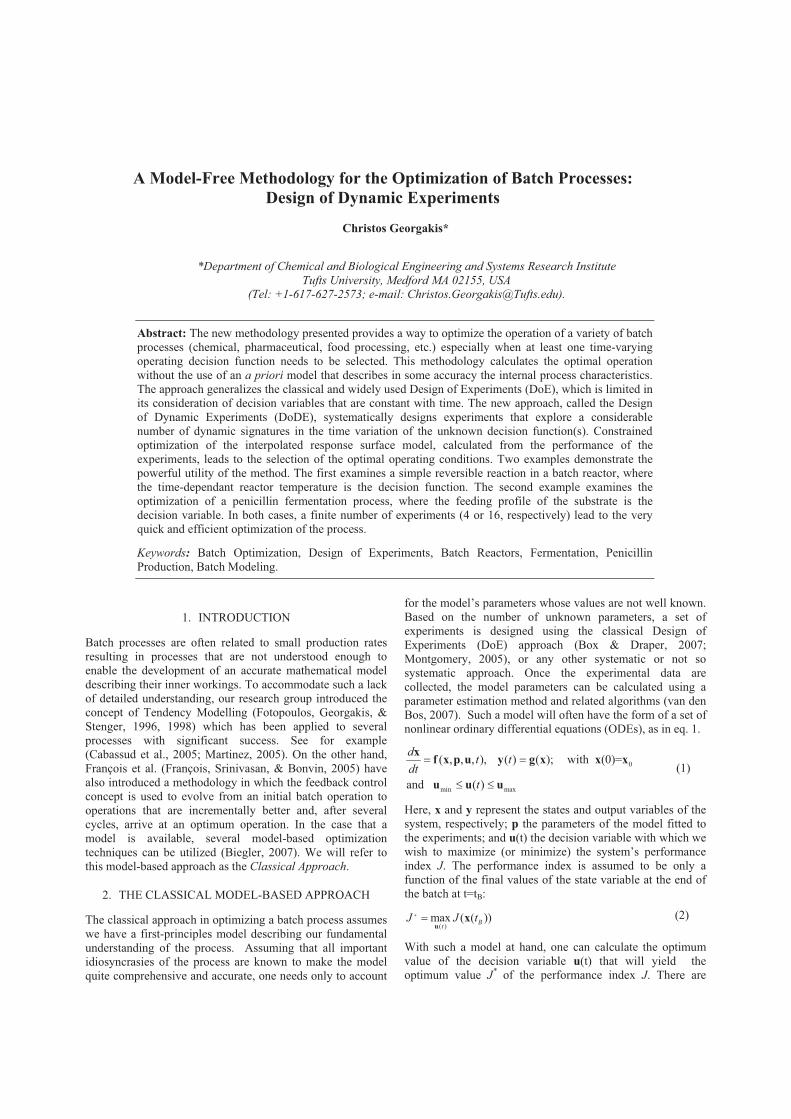
The simplest set of DoDE experiments is obtained by selecting the smallest value of N in eq. (3), equal to two. This implies that the dynamic profile of u(�), or the coded variable w(�), is a linear combination of the first two Legendre polynomials P0(�) and P1(�). This limits our consideration among constant or linear time dependencies. In deciding the values of the a1 and a2 sub-factors we can follow the classical DoE approach. If we do level-2 experiments for each sub-factor, we will design the following 22=4 experiments:

1

2

1 1 1 1, , ,

1 1 1 1aa

� � � � � � � � � � �� � � � � � � �� � � �� � � � � � � �� � � �

� (9)�

Translating, for example, the second experiment to the corresponding dynamic coded variable w(�) we have

0 1( ) ( ) ( ) 2w P P� � � �� � � . We realize that this profile does not meet its constraints 1 ( ) 1w �� � � � . This is easily remedied by imposing the following constraints on the a1 and a2 constants: 1 21 1a a� � � � � and 1 21 1a a� � � � � reducing the values of a1 and a2, without changing their relative magnitude so the that the constraints on w(�) are met. This leads to the following design of experiments

1

2

0.5 0.5 0.5 0.5, , ,

0.5 0.5 0.5 0.5aa

� � � � � � � � � � �� � � � � � � �� � � �� � � � � � � �� � � �

(10)

In this case, the four time-variations in w(�) are shown in Figure 1.

Figure 1: The 22=4 DoDE experiments

4.2. Other DoDE Examples

For N=3, we are considering the first three Legendre polynomials, and if we consider only low and high values, we need to perform 23= 8 experiments. Here we are considering quadratic dependence on time along with the constant and linear sub-factors considered before. If we add cubic dependence by letting N=4 we need 24= 16 experiments and the use of the next Legendre polynomial:

3 23 ( ) 20 30 12 1P � � � �� � � � � . For N=5 we involve the first

five shifted Legendre polynomials. This includes the four polynomials mentioned above along with the fifth one:

4 3 24 ( ) 70 -140 90 - 20 1P � � � � �� � � . Here we need 25= 32

experiments. In the case we design level-3 full factorial experiments we need 32= 9 experiments for N=2, and 33= 27 experiments for N=3.

We should note that the way the dynamic experiments are designed involves two steps that are similar to the ones presented in section 4.1 for the simplest of the DoDE designs. In the first step, the sub-factors related to the values of the coefficients ai are treated as independent from each other and are assigned initial values of (-1 , +1) in the level 2 designs and values (-1, 0, +1) in the lever 3 designs. In the second

0 0. 0. 0. 0. 0. 0. 0. 0. 0. 1-1

-0.8

-0.6

-0.4

-0.2

0

0.

0.

0.

0.

1

Dimensionless Time = Time / Batch

Cod

ed v

aria

ble

The 4 Experiments of the 2^2 DoDE design

Table 1: Details of the Batch Reactor Optimization using the DoDE Methodology

Dyn

amic

Su

b-fa

ctor

s Le

vels

Cas

e N

umbe

r an

d N

umbe

r of

Ex

perim

ents

Bes

t C

onve

rsio

n fr

om In

itial

2n o

r 3n E

xper

imen

ts

Best Profile from the Initial 2n or 3n Experiments:

T(�)=308+15u(�) oK with u(�)=a1P0+a2P1+a3P3+…

RSM

-Opt

imum

C

onve

rsio

n of

A

Defining Parameters of the Calculated

RSM-Optimum Profile w(�)

Level 2 FULL Factorial Designs

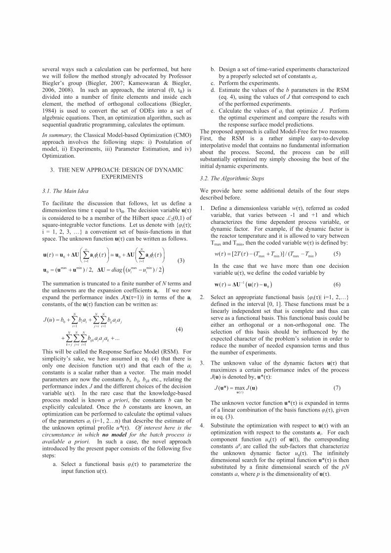
1 2 DA1:21= 2 62.32% a1 = -1 62.23% a1 = -1 2 2 DA2 : 22= 4 73.46% (a1, a2) = (-0.5, 0.5) 76.57% (a1, a2) = (0, 1) 3 2 DA3: 23= 8 74.61% (a1, a2, a3) = (-0.3, 0.3, -0.3) 77.77% (a1, a2, a3) = (0, 1, 0) 4 2 DA4: 24=16 74.82% (a1, a2, a3, a4) = (-0.3, 0.3, -0.3, 0.3) 78.10% (a1, a2, a3, a4) = (0, 1, 0,- 0.04) 5 2 DA5: 25=32 74.43% (a1, a2, a3, a4, a5) = (-0.3, 0.3, -0.3, 0.3, .3) 78.43% (a1, a2, a3, a4, a5) = (0, 0.9, 0,- 0.08, -0.2)

Level 3 FULL Factorial Designs

1 3 DA6 31= 3 73.91% a1 = 0 73.92% a1 = -0.03 2 3 DA7 32= 9 77.35% (a1, a2) = (0, 1) 77.57% (a1, a2) = (0.1, 0.9) 3 3 DA8 33=27 77.35% (a1, a2, a3) = (0, 1, 0) 77.66% (a1, a2, a3) = (0.05, 0.9, 0.06)

step, all of the ai values related to a single experiment are scaled up or, in most cases, down by a common factor, so that the coded dynamic variable w(�) attains values that are inside the [-1, +1] interval. Making the maximum (or minimum) of each profile touch the maximum (or minimum) values of w(�) also ensures that the set of DoDE experiments covers all areas on the [-1, +1] x [0, 1] rectangle.

5. BATCH REACTOR WITH REVERSIBLE REACTION

Here we consider the optimization of the operation of a batch reactor in which a reversible reaction between reactant A and product B takes place with the following characteristics:

1

21 A 2 B

1 10 1 2 20 2

7 1310 20 1 2

; k C -k C

k exp( / ) [1/hr]; k exp( / ) [1/hr]

k =1.32x10 ; k =5.24x10 ; 10,000; 20,000

k

kA B r with

k E RT k E RT

E E

��� ����

� � � �

� �

We select the activation energy of the reverse reaction to be larger than that for the forward reaction. This leads to the expectation that the optimum temperature profile is a decreasing one (Rippin, 1983). One needs to note here, that for the development of the fundamental model above, we need to assume that the first order kinetic rate is correct. We then perform at least 4 experiments to estimate the values of k10, k20, E1, and E2.

With such a model at hand, one can optimize the reactor temperature profile to maximize the conversion of reactant A. This is achieved by converting the ODEs into algebraic equations via Radau collocation on finite elements (Biegler, 2007). The reactor temperature is constrained between 20 0C and 50 0C and the optimization is achieved by use of the IPOPT algorithm (Wächter & Biegler, 2006).

The optimum profile calculated is constant at the upper temperature constraint for almost 0.4 hrs and then decreases to the minimum constraint at the end of the batch. We select here to fix the batch time to 2.5 hrs and the maximum conversion of the reactant A is calculated to be 77.68%. In

Table 1, the results of the different DoDE experiments are presented. They involve up to 5 dynamic sub-factors and include level-2 (low-high) and level-3 (low-medium-high) experiments. In the fourth column the best conversion value of the initial runs is given. In the second to last column, the expected best batch performance, as calculated by the optimization of the response surface model (RSM), is given. In the last column the characteristics of this RSM-optimal profile is given in terms of the coded variable:

1 0 2 1( ) ( ) ( ) ...w a P a P� � �� � � The temperature profile can then be calculated by eq. 5. We observe that in the case denoted as DA2 in Table 1 only four experiments described in Figure 1 yield an RSM-optimum with a conversion of 76.57% which is just 1.43% away from the true optimum of 77.68%. We also observe that a larger number of experiments, such as those of cases DA4, DA5, DA7 and DA8, predict a higher conversion, even closer to the true optimum. However, as the number of experiments performed increases, the changes in the predicted optimum conversion becomes smaller and smaller per additional experiment, implying that the true optimum has been reached.

6. PENICILLIN FERMENTATION

Here we simulate the penicillin fermentation model of Bajpai and Reuss (Bajpai & Reuss, 1980) which has been the center of attention in several model-based optimizations (Riascos & Pinto, 2004). The model used to simulate the experiment consists of the equations in the Appendix. To focus on the main idea of calculating the optimum time-varying profile, we fix the batch time to tb=130 hrs and the growth phase of the biomass to tf=30 hrs. Here we want to demonstrate the application of the DoDE approach to this challenging optimization problem to demonstrate its power in optimizing complex processes. For this reason, we are not designing experiments that vary the tf and tb values, since they are not time-varying decision variables or factors.

We choose to design 16 experiments with 4=22 variations for the substrate flow in growth phase 0�t�tf (or 0����; �=tf/tb)

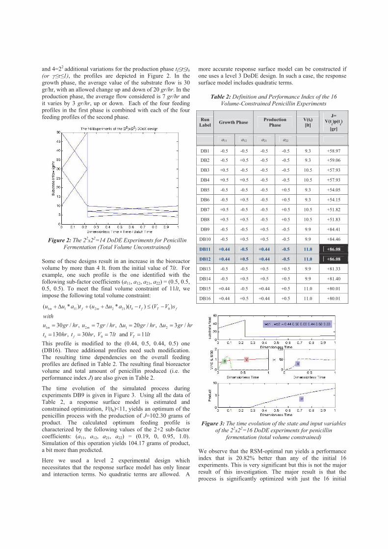
and 4=22 additional variations for the production phase tf�t�tb (or ����1), the profiles are depicted in Figure 2. In the growth phase, the average value of the substrate flow is 30 gr/hr, with an allowed change up and down of 20 gr/hr. In the production phase, the average flow considered is 7 gr/hr and it varies by 3 gr/hr, up or down. Each of the four feeding profiles in the first phase is combined with each of the four feeding profiles of the second phase.

Figure 2: The 22x22=14 DoDE Experiments for Penicillin

Fermentation (Total Volume Unconstrained)

Some of these designs result in an increase in the bioreactor volume by more than 4 lt. from the initial value of 7lt. For example, one such profile is the one identified with the following sub-factor coefficients (a11, a12, a21, a22) = (0.5, 0.5, 0.5, 0.5). To meet the final volume constraint of 11lt, we impose the following total volume constraint:

1 1 11 2 2 21 0

1 2 1 2

0

( * ) ( * )( ) ( )

30 / , 7 / , 20 / , 3 /

130 , 30 , 7 and 11

m f m b f T f

m m

b f T

u u a t u u a t t V V swithu gr hr u gr hr u gr hr u gr hrt hr t hr V lt V lt

� � � � � � � �

� � � � � �� � � �

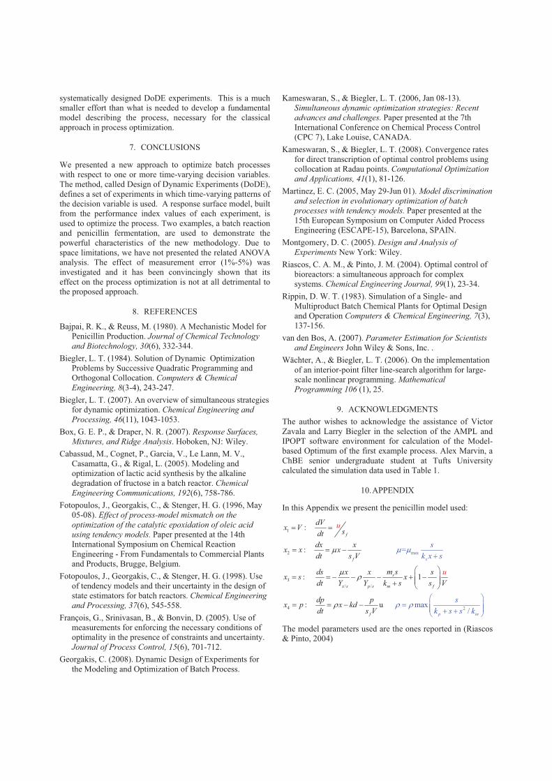
This profile is modified to the (0.44, 0.5, 0.44, 0.5) one (DB16). Three additional profiles need such modification. The resulting time dependencies on the overall feeding profiles are defined in Table 2. The resulting final bioreactor volume and total amount of penicillin produced (i.e. the performance index J) are also given in Table 2.

The time evolution of the simulated process during experiments DB9 is given in Figure 3. Using all the data of Table 2, a response surface model is estimated and constrained optimization, V(tb)<11, yields an optimum of the penicillin process with the production of J=102.30 grams of product. The calculated optimum feeding profile is characterized by the following values of the 2+2 sub-factor coefficients: (a11, a12, a21, a22) = (0.19, 0, 0.95, 1.0). Simulation of this operation yields 104.17 grams of product, a bit more than predicted.

Here we used a level 2 experimental design which necessitates that the response surface model has only linear and interaction terms. No quadratic terms are allowed. A

more accurate response surface model can be constructed if one uses a level 3 DoDE design. In such a case, the response surface model includes quadratic terms.

Table 2: Definition and Performance Index of the 16 Volume-Constrained Penicillin Experiments

Run Label Growth Phase Production

Phase V(tf) [lt]

J= V(t

f)p(t

f)

[gr]

a11 a12 a21 a22

DB1 -0.5 -0.5 -0.5 -0.5 9.3 +58.97

DB2 -0.5 +0.5 -0.5 -0.5 9.3 +59.06

DB3 +0.5 -0.5 -0.5 -0.5 10.5 +57.93

DB4 +0.5 +0.5 -0.5 -0.5 10.5 +57.93

DB5 -0.5 -0.5 -0.5 +0.5 9.3 +54.05

DB6 -0.5 +0.5 -0.5 +0.5 9.3 +54.15

DB7 +0.5 -0.5 -0.5 +0.5 10.5 +51.82

DB8 +0.5 +0.5 -0.5 +0.5 10.5 +51.83

DB9 -0.5 -0.5 +0.5 -0.5 9.9 +84.41

DB10 -0.5 +0.5 +0.5 -0.5 9.9 +84.46

DB11 +0.44 -0.5 +0.44 -0.5 11.0 +86.08

DB12 +0.44 +0.5 +0.44 -0.5 11.0 +86.08

DB13 -0.5 -0.5 +0.5 +0.5 9.9 +81.33

DB14 -0.5 +0.5 +0.5 +0.5 9.9 +81.40

DB15 +0.44 -0.5 +0.44 +0.5 11.0 +80.01

DB16 +0.44 +0.5 +0.44 +0.5 11.0 +80.01

Figure 3: The time evolution of the state and input variables

of the 22x22=16 DoDE experiments for penicillin fermentation (total volume constrained)

We observe that the RSM-optimal run yields a performance index that is 20.82% better than any of the initial 16 experiments. This is very significant but this is not the major result of this investigation. The major result is that the process is significantly optimized with just the 16 initial

systematically designed DoDE experiments. This is a much smaller effort than what is needed to develop a fundamental model describing the process, necessary for the classical approach in process optimization.

7. CONCLUSIONS

We presented a new approach to optimize batch processes with respect to one or more time-varying decision variables. The method, called Design of Dynamic Experiments (DoDE), defines a set of experiments in which time-varying patterns of the decision variable is used. A response surface model, built from the performance index values of each experiment, is used to optimize the process. Two examples, a batch reaction and penicillin fermentation, are used to demonstrate the powerful characteristics of the new methodology. Due to space limitations, we have not presented the related ANOVA analysis. The effect of measurement error (1%-5%) was investigated and it has been convincingly shown that its effect on the process optimization is not at all detrimental to the proposed approach.

8. REFERENCES

Bajpai, R. K., & Reuss, M. (1980). A Mechanistic Model for Penicillin Production. Journal of Chemical Technology and Biotechnology, 30(6), 332-344.

Biegler, L. T. (1984). Solution of Dynamic Optimization Problems by Successive Quadratic Programming and Orthogonal Collocation. Computers & Chemical Engineering, 8(3-4), 243-247.

Biegler, L. T. (2007). An overview of simultaneous strategies for dynamic optimization. Chemical Engineering and Processing, 46(11), 1043-1053.

Box, G. E. P., & Draper, N. R. (2007). Response Surfaces, Mixtures, and Ridge Analysis. Hoboken, NJ: Wiley.

Cabassud, M., Cognet, P., Garcia, V., Le Lann, M. V., Casamatta, G., & Rigal, L. (2005). Modeling and optimization of lactic acid synthesis by the alkaline degradation of fructose in a batch reactor. Chemical Engineering Communications, 192(6), 758-786.

Fotopoulos, J., Georgakis, C., & Stenger, H. G. (1996, May 05-08). Effect of process-model mismatch on the optimization of the catalytic epoxidation of oleic acid using tendency models. Paper presented at the 14th International Symposium on Chemical Reaction Engineering - From Fundamentals to Commercial Plants and Products, Brugge, Belgium.

Fotopoulos, J., Georgakis, C., & Stenger, H. G. (1998). Use of tendency models and their uncertainty in the design of state estimators for batch reactors. Chemical Engineering and Processing, 37(6), 545-558.

François, G., Srinivasan, B., & Bonvin, D. (2005). Use of measurements for enforcing the necessary conditions of optimality in the presence of constraints and uncertainty. Journal of Process Control, 15(6), 701-712.

Georgakis, C. (2008). Dynamic Design of Experiments for the Modeling and Optimization of Batch Process.

Kameswaran, S., & Biegler, L. T. (2006, Jan 08-13). Simultaneous dynamic optimization strategies: Recent advances and challenges. Paper presented at the 7th International Conference on Chemical Process Control (CPC 7), Lake Louise, CANADA.

Kameswaran, S., & Biegler, L. T. (2008). Convergence rates for direct transcription of optimal control problems using collocation at Radau points. Computational Optimization and Applications, 41(1), 81-126.

Martinez, E. C. (2005, May 29-Jun 01). Model discrimination and selection in evolutionary optimization of batch processes with tendency models. Paper presented at the 15th European Symposium on Computer Aided Process Engineering (ESCAPE-15), Barcelona, SPAIN.

Montgomery, D. C. (2005). Design and Analysis of Experiments New York: Wiley.

Riascos, C. A. M., & Pinto, J. M. (2004). Optimal control of bioreactors: a simultaneous approach for complex systems. Chemical Engineering Journal, 99(1), 23-34.

Rippin, D. W. T. (1983). Simulation of a Single- and Multiproduct Batch Chemical Plants for Optimal Design and Operation Computers & Chemical Engineering, 7(3), 137-156.

van den Bos, A. (2007). Parameter Estimation for Scientists and Engineers John Wiley & Sons, Inc. .

Wächter, A., & Biegler, L. T. (2006). On the implementation of an interior-point filter line-search algorithm for large-scale nonlinear programming. Mathematical Programming 106 (1), 25.

9. ACKNOWLEDGMENTS The author wishes to acknowledge the assistance of Victor Zavala and Larry Biegler in the selection of the AMPL and IPOPT software environment for calculation of the Model-based Optimum of the first example process. Alex Marvin, a ChBE senior undergraduate student at Tufts University calculated the simulation data used in Table 1.

10.APPENDIX

In this Appendix we present the penicillin model used:

max

1

2

3/ /

4 2

:

:

:

=

max/

1

: u

x

p

f

f

s

x s p s m

if n

f

dVx V sdtdx xx x xdt s V

m sds x x sx

s

s xdt Y Y k s s V

dp px p x kddt s

k x s

sk s s k

u

u

V

�

� �

� �

� � �

� �

� � �

�� � � � � � � � �� � �

�

�

�� � �� ��

��

� �

The model parameters used are the ones reported in (Riascos & Pinto, 2004)