A mixed model QTL analysis for sugarcane multiple-harvest-location trial data

ORIGINAL PAPER

A mixed model QTL analysis for sugarcanemultiple-harvest-location trial data

M. M. Pastina • M. Malosetti • R. Gazaffi • M. Mollinari •

G. R. A. Margarido • K. M. Oliveira • L. R. Pinto •

A. P. Souza • F. A. van Eeuwijk • A. A. F. Garcia

Received: 19 November 2010 / Accepted: 28 October 2011 / Published online: 13 December 2011

� The Author(s) 2011. This article is published with open access at Springerlink.com

Abstract Sugarcane-breeding programs take at least

12 years to develop new commercial cultivars. Molecular

markers offer a possibility to study the genetic architecture

of quantitative traits in sugarcane, and they may be used in

marker-assisted selection to speed up artificial selection.

Although the performance of sugarcane progenies in

breeding programs are commonly evaluated across a range

of locations and harvest years, many of the QTL detection

methods ignore two- and three-way interactions between

QTL, harvest, and location. In this work, a strategy for

QTL detection in multi-harvest-location trial data, based on

interval mapping and mixed models, is proposed and

applied to map QTL effects on a segregating progeny from

a biparental cross of pre-commercial Brazilian cultivars,

evaluated at two locations and three consecutive harvest

years for cane yield (tonnes per hectare), sugar yield

(tonnes per hectare), fiber percent, and sucrose content. In

the mixed model, we have included appropriate (co)vari-

ance structures for modeling heterogeneity and correlation

of genetic effects and non-genetic residual effects. Forty-

six QTLs were found: 13 QTLs for cane yield, 14 for sugar

yield, 11 for fiber percent, and 8 for sucrose content. In

addition, QTL by harvest, QTL by location, and QTL by

harvest by location interaction effects were significant for

all evaluated traits (30 QTLs showed some interaction, and

16 none). Our results contribute to a better understanding

of the genetic architecture of complex traits related to

biomass production and sucrose content in sugarcane.

Keywords Polyploids � Outcrossing species � Integrated

linkage map � QTL 9 E

Introduction

Sugarcane (Saccharum spp.) is a clonally propagated out-

crossing polyploid crop of great importance in tropical

agriculture as a source of sugar and bioethanol. Modern

commercial sugarcane cultivars are derived from inter-

specific crosses between Saccharum officinarum (basic

chromosome number: x = 10; 2n = 8x = 80) and its wild

relative S. spontaneum (x = 8; 5x B 2n B 16x), followed

by few cycles of intercrossing and selection. Due to the

intercrossings, these modern cultivars have chromosome

Electronic supplementary material The online version of thisarticle (doi:10.1007/s00122-011-1748-8) contains supplementarymaterial, which is available to authorized users.

Communicated by A. Charcosset.

M. M. Pastina � R. Gazaffi � M. Mollinari �G. R. A. Margarido � A. A. F. Garcia (&)

Departamento de Genetica, Escola Superior de Agricultura Luiz

de Queiroz (ESALQ), Universidade de Sao Paulo (USP), CP 83,

13400-970 Piracicaba, SP, Brazil

e-mail: [email protected]

M. Malosetti � F. A. van Eeuwijk

Biometris, Wageningen University, P.O. Box 100, 6700 AC

Wageningen, The Netherlands

K. M. Oliveira

Centro de Tecnologia Canavieira (CTC), CP 162, 13400-970

Piracicaba-SP, Brazil

L. R. Pinto

Centro Avancado da Pesquisa Tecnologica do Agronegocio de

Cana, IAC/Apta, CP 206, 14001-970 Ribeirao Preto, SP, Brazil

A. P. Souza

Centro de Biologia Molecular e Engenharia Genetica (CBMEG),

Departamento de Genetica e Evolucao, Universidade Estadual de

Campinas (UNICAMP), Cidade Universitaria Zeferino Vaz, CP

6010, 13083-875 Campinas, SP, Brazil

123

Theor Appl Genet (2012) 124:835–849

DOI 10.1007/s00122-011-1748-8

number in somatic cells (2n) ranging from 100 to 130

(D’Hont et al. 1998; Irvine 1999; Grivet and Arruda 2001;

D’Hont 2005; Piperidis et al. 2010).

Quantitative trait loci (QTL) mapping is a useful tool to

dissect and to understand the genetic architecture of complex

traits. However, two main complicating factors make QTL

mapping more challenging in sugarcane than other species.

(1) Ploidy level: the polyploidy and aneuploidy nature of

sugarcane cultivars cause a complex pattern of chromosomal

segregation in meiosis (Heinz and Tew 1987); (2) Outbred

parents: since sugarcane inbred lines are not available,

linkage map construction and QTL mapping rely on segre-

gating progenies derived from biparental cross of highly

heterozygous outbred parents. These two factors combined

enable the appearance of different allele dosages (copy

number variation) in each locus (marker or QTL), therefore,

a mixture of segregating patterns can be observed in the

segregating progenies (Ripol et al. 1999; Wu et al. 2002a, b;

Lin et al. 2003). Moreover, due to the usage of outbred

parents, linkage phases between markers are unknown.

The estimation of genetic linkage maps in sugarcane

started after the development of single-dose markers

(SDMs) (Wu et al. 1992). In a biparental cross, an SDM has

either a single copy of an allele in one parent only or a single

copy of the same allele in both parents, thus segregating in

1:1 (presence : absence) or 3:1 (presence:absence) ratio,

respectively. The double pseudo-testcross strategy uses

SDMs segregating in 1:1 ratio for each parent separately to

build two independent genetic maps (one for each parent)

for any cross between heterozygous parents with bivalent

pairing in meiosis (Grattapaglia and Sederoff 1994; Por-

ceddu et al. 2002; Shepherd et al. 2003; Carlier et al. 2004;

Chen et al. 2008; Cavalcanti and Wilkinson 2007). In spite

of the relative success of the double pseudo-testcross

strategy in sugarcane (for example, Al-janabi et al. 1993;

Ming et al. 1998; Hoarau et al. 2001; McIntyre et al.

2005a), an integrated map combining SDMs segregating in

1:1 and 3:1 ratio (Garcia et al. 2006; Oliveira et al. 2007)

permits better genome saturation and characterization of the

polymorphic variation in the biparental cross, therefore,

being a more realistic framework for QTL mapping.

Although many statistical methods have been specifi-

cally developed to map QTLs in outcrossing species (Knott

and Haley 1992; Haley et al. 1994; Schafer-Pregl et al.

1996; Knott et al. 1997; Sillanpaa and Arjas 1999; Lin et al.

2003; Wu et al. 2007; Hu and Xu 2009), the general double

pseudo-testcross method has been widely used to study

QTL in sugarcane through single marker analysis (SM),

interval mapping (IM) and composite interval mapping

(CIM) (Sills et al. 1995; Daugrois et al. 1996; Ming et al.

2001; 2002a, b; Hoarau et al. 2002; Jordan et al. 2004; da

Silva and Bressiani 2005; McIntyre et al. 2005a, b, 2006;

Reffay et al. 2005; Aitken et al. 2006, 2008; Raboin et al.

2006; Al-Janabi et al. 2007; Piperidis et al. 2008; Pinto

et al. 2010; Pastina et al. 2010). In this approach, statistical

analyses are carried out with the well-established backcross

model using softwares developed for inbred-based popula-

tions. However, for the reasons stated previously, an inte-

grated-map-based model might be a better choice for

outcrossing species, such as sugarcane.

In addition to its genetic complexity, sugarcane is a

perennial crop, in which individuals are usually harvested in

multiple years. Thus, traits are often repeatedly measured

not only across different locations but also along successive

years (harvests), adding a time dimension to the phenotypic

data. Quantitative-trait-based sugarcane varietal selection is

commonly based on information from a series of field trials,

considering different harvests and locations, here called

multi-harvest-location trials (MHLT). QTL studies in sug-

arcane usually are carried out for each harvest-location trial

separately, ignoring QTL-by-harvest (QTL 9 H), QTL-

by-location (QTL 9 L) and QTL-by-harvest-by-location

(QTL 9 H 9 L) interactions (Hoarau et al. 2002; Jordan

et al. 2004; McIntyre et al. 2005b; Reffay et al. 2005; Pinto

et al. 2010; Pastina et al. 2010). The use of statistical

models that allow the identification of stable QTL across

different environments (an environment is any combination

of location and harvest) can provide powerful and useful

information for breeding purposes, such as breeding values

in marker-assisted selection (MAS).

Mixed models have been successfully employed to study

genotype-by-environment (G 9 E) interaction (Denis et al.

1997; Piepho 1997; Cullis et al. 1998; Chapman 2008;

Smith et al. 2001, 2007; van Eeuwijk et al. 2007), as well as

QTL-by-environment (QTL 9 E) interaction (Piepho 2000,

2005; Verbyla et al. 2003; Malosetti et al. 2004, 2008; van

Eeuwijk et al. 2005; Boer et al. 2007; Mathews et al. 2008).

They provide great flexibility to represent the complex

variance-covariance structures that follow from the patterns

of genetic correlations between harvests and locations. In

this article, we propose a mixed model QTL mapping

strategy for sugarcane, paying special attention to model

dependencies (correlations) between harvests and locations,

which allows us to find stable QTLs that can be distin-

guished from environment-sensitive QTLs.

Materials and methods

Plant material

Phenotypic and molecular data were collected in a segre-

gating population of 100 individuals derived from a cross

between two pre-commercial Brazilian cultivars, SP80-180

(B3337 9 polycross) and SP80-4966 (SP71-1406 9 poly-

cross). SP80-180 was the female parent and had lower

836 Theor Appl Genet (2012) 124:835–849

123

sucrose content and high stalk production, whereas SP80-

4966 (male parent) had higher sucrose and lower stalk

production. Both parents and population were developed at

the Experimental Station of the Centro de Tecnologia

Canavieira (CTC), Camamu county, State of Bahia, Brazil.

Molecular data

Restriction fragment length polymorphism (RFLP), RFLP

and simple sequence repeat (SSR) markers derived from

expressed sequence tag (EST-RFLP and EST-SSR) were

used to genotype parents and progeny. All these markers

had already been generated and coded, as detailed in

Garcia et al. (2006) and Oliveira et al. (2007). Each seg-

regating allele was scored as a dominant marker, based on

its presence or absence in the progeny. Only SDMs were

considered. The observed segregation pattern of each

marker was tested against its expected ratio using chi-

square tests (v2): 1:1 if it is a SDM present in only one

parent or 3:1 if it is a SDM present in both parents. All loci

with strong deviations from expected proportions were

discarded after Bonferroni correction.

Phenotypic data

The mapping population was planted in 2003 at two

locations (Piracicaba and Jau, both in the State of Sao

Paulo, Brazil), and evaluated in the first, second and third

harvest years for cane yield (tonnes of cane per hectare,

TCH), sugar yield (tonnes of sugar per hectare, TSH), fiber

percent and sucrose content (Pol). In each location, the

experimental design consisted of an augmented random-

ized complete block design with two replicates. However,

genotypes were not fully randomized within blocks, instead

they were randomly split into three groups with 36, 38, and

26 individuals each. Then, individuals were randomized

within each group, but groups were not randomized within

blocks. In the experiments, each group of individuals was

augmented by four checks (commercial cultivars SP80-

1842, SP81-3250, SP80-1816 and RB72454). Both parents

were also included in one of the groups, but not considered

in the statistical analysis.

Linkage map

Based on a multipoint approach (Wu et al. 2002a, b), map

construction was carried out using the OneMap package

(Margarido et al. 2007). For this purpose, 741 molecular

markers were used, including 459 loci displaying an 1:1

segregation ratio (100 RFLP, 27 EST-RFLP, 332 EST-

SSR) and 282 loci segregating in a 3:1 ratio (88 RFLP, 10

EST-RFLP, 184 EST-SSR). Following the notation in Wu

et al. (2002a), markers segregating for the parent SP80-180

(P1) were denoted by D1, corresponding to the configura-

tion ‘ao 9 oo’, in which the a allele is dominant over the

o (null) allele. Informative loci for the parent SP80-4966

(P2) were denoted by D2, with the configuration ‘oo 9 ao’,

and markers segregating for both parents were denoted by

C, with configuration ‘ao 9 ao’. Markers were assigned to

linkage groups (LGs) based on two point analysis, con-

sidering a minimum LOD threshold of 6. LGs with a

maximum of five loci were ordered through the comparison

of all possible orders, in a procedure analogous to the

compare command in the MAPMAKER/EXP software

(Lander et al. 1987). For LGs with more than 5 markers,

the order algorithm started with the five most informative

markers, which were ordered through the comparison of all

possible orders, and then the other markers were sequen-

tially placed on the LG at the position with largest likeli-

hood, in a similar way to that performed by the try

command in the MAPMAKER/EXP software. Afterward,

the ripple command was applied to verify if local inver-

sions had occurred. Map distances were expressed in cen-

tiMorgans (cM) based on the Kosambi function (Kosambi

1944). LGs were assembled into putative homology groups

(HGs) when at least two loci (from the same or different

marker type: RFLP, EST-RFLP or EST-SSR) were shared

(Jannoo et al. 2004; Okada et al. 2010).

Genetic predictors

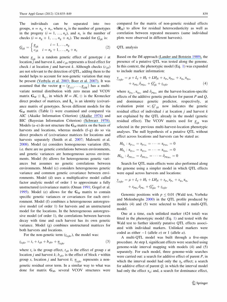
For notation purposes, in a similar way to that proposed by

Lin et al. (2003), consider a full-sib progeny obtained from

a cross between two outbred diploid parents, denoted as

P and Q (Fig. 1). The illustration in Fig. 1 could be seen as

a general case when compared with loci configuration

observed in sugarcane, where only SDMs were considered.

The genotypes of two adjacent markers m and m ? 1 can

be represented by Pm{1,2}, Qm

{1,2}, Pm?1{1,2} and Qm?1

{1,2}, in which

{1, 2} indicates the allelic possibilities for each locus.

However, since we are using dominant markers, we

let allele 2 in parents P and Q representing possibly a series

of alleles in polyploid species. Allele 2 could be thought as

‘‘all but allele 1’’. Suppose that there is a QTL between

these two markers, with alleles P1 and P2 for parent P, Q1

and Q2 for parent Q. Thus, QTL segregation in the progeny

will fit into four genotypic classes (P1Q1, P1Q2, P2Q1 and

P2Q2), with an 1:1:1:1 ratio. Therefore, it is possible to

define three orthogonal contrasts involving these four

genotypic classes (Lin et al. 2003; Gazaffi 2009):

ap ¼ P1Q1 þ P1Q2 � P2Q1 � P2Q2

aq ¼ P1Q1 � P1Q2 þ P2Q1 � P2Q2

dpq ¼ P1Q1 � P1Q2 � P2Q1 þ P2Q2

Theor Appl Genet (2012) 124:835–849 837

123

The first and second contrasts relate to additive QTL

effects in parents P and Q respectively, while the third

refers to dominance effect (intra-locus interaction) between

the additive effects in each parent. Genetic predictors were

constructed for a discrete grid of evaluation points

(w) along the genome (w = 1, …, W). These genetic pre-

dictors were used as explanatory variables in the mixed

models. For individual i and evaluation point w, the genetic

predictors are:

xpiw ¼ pðP1Q1jMiÞ þ pðP1Q2jMiÞ� pðP2Q1jMiÞ � pðP2Q2jMiÞ

xqiw ¼ pðP1Q1jMiÞ � pðP1Q2jMiÞþ pðP2Q1jMiÞ � pðP2Q2jMiÞ

xpqiw ¼ pðP1Q1jMiÞ � pðP1Q2jMiÞ� pðP2Q1jMiÞ þ pðP2Q2jMiÞ

where xpiw; xqiw and xpqiw are the expected values of ap, aq

and dpq respectively, conditional on all marker information

Mi in a particular LG (Haley and Knott 1992; Martınez

andCurnow 1992; Lynch and Walsh 1998). The condi-

tional multipoint probabilities pðP1Q1jMiÞ; pðP1Q2jMiÞ;pðP2Q1jMiÞ and pðP2Q2jMiÞ were calculated via hidden

Markov chain model (OneMap package, Margarido et al.

2007) for all marker positions and discrete grid of evalu-

ation points with step size of 1 cM along the genome.

Due to the lack of information of SDMs (i.e. only 1:1

and 3:1 segregation patterns could be obtained), some

genetic predictors could be linear combinations of others at

some genomic positions, therefore, the matrix of genetic

predictors could be singular. Since collinearity could cause

serious problems with estimation and interpretation of

parameters, its presence was investigated by examining the

singular values and the condition number of the matrix of

genetic predictors at all genomic positions. Only informa-

tive contrasts (without collinearity) were then considered.

For example, LGs with only marker type D1 have enough

information solely for the estimation of one contrast for the

additive effect in parent P. The same principle was applied

to all LGs and genomic positions.

Multi-harvest-location phenotypic analysis

Prior to QTL detection, the identification of an appropriate

mixed model for the phenotypic data was done by com-

paring different structures of variance-covariance (VCOV)

matrix for the genetic effects (Table 1). For mathematical

description of the model, a notation similar to that pre-

sented by Eckermann et al. (2001), Verbyla et al. (2003)

and Boer et al. (2007) was used. The statistical model, in

which the underlining indicates a random variable, is:

yisjkr¼ lþ Lj þ Hk þ LHjk þ Gijk þ eisjkr ð1Þ

yisjkr

is the phenotype of the rth replicate (r = 1, 2) of

the ith individual (i ¼ 1; 2; . . .; n) of group s (s = 1, 2, 3)

in location j (j = 1, J = 2) and harvest k

(k = 1, 2, K = 3); l is the overall mean; Lj is the location

effect; Hk is the harvest effect; LHjk is the location by

harvest interaction effect; Gijk is the effect of individual i at

location j and harvest k; and eisjkr is a non-genetic effect.

Fig. 1 Graphical representation of a biparental cross between

outbred parents P and Q. Pm{1,2}, Qm

{1,2}, Pm?1{1,2} and Qm?1

{1,2} are the

marker alleles for loci m and m ? 1; P1, P2, Q1 and Q2 are the QTL

alleles

Table 1 Examined models for the genetic (co)variance matrix (GM)

GM matrix Model nPARa Description

GM = GM 9 ML-H (a) ID 1 Identical genetic variation

(b) DIAG M Heterogeneous genetic variation

(c) CSHet M ? 1 Compound symmetry with heterogeneous genetic variation

(d) FA1 2M First-order factor analytic model

(e) US MðMþ1Þ2

Unstructured model

GM = GJ 9 JL � GK 9 K

H (f) US � AR1HetJðJþ1Þþ2ðKþ1Þ

2� 1 Unstructured and first-order autoregressive models for locations and harvests,

respectively

(g) US � US JðJþ1ÞþKðKþ1Þ2

� 1 Unstructured models for locations and harvests

Models (a–e) use the factorial combination of locations and harvests as different environments. Models (f–g) use the direct product of

(co)variance matrices for locations and harvestsa The number of parameters for the models (f–g) follows from the sum of the parameters for the component matrices minus the number of

identification constraints. M = JK, where J is the number of locations and K is the number of harvests.

838 Theor Appl Genet (2012) 124:835–849

123

The individuals can be separated into two

groups, n = ng ? nc, where ng is the number of genotypes

in the progeny (i = 1, …, ng), and nc is the number of

checks (i = ng ? 1, …, ng ? nc). The model for Gijk is:

Gijk ¼g

ijki ¼ 1; . . .; ng

cijk i ¼ ng þ 1; . . .; ng þ nc

�ð2Þ

where gijk

is a random genetic effect of genotype i at

location j and harvest k, and cijk represents a fixed effect for

check i at location j and harvest k. Although checks (cijk)

are not relevant to the detection of QTL, adding them to the

model helps to account for non-genetic variation that may

be present (Verbyla et al. 2003; Boer et al. 2007). It was

assumed that the vector g ¼ ðg111; . . .; g

IJKÞ has a multi-

variate normal distribution with zero mean and VCOV

matrix GM � Ing; in which M = JK, � is the Kronecker

direct product of matrices, and Ingis an identity (co)vari-

ance matrix of genotypes. Seven different models for the

GM matrix (Table 1) were examined and compared via

AIC (Akaike Information Criterion) (Akaike 1974) and

BIC (Bayesian Information Criterion) (Schwarz 1978).

Models (a–e) do not structure the GM matrix on the basis of

harvests and locations, whereas models (f–g) do so via

direct products of (co)variance matrices for locations and

harvests separately (Smith et al. 2007; Malosetti et al.

2008). Model (a) considers homogeneous variation (ID),

i.e. there are no genetic correlations between environments,

and genetic variances are homogeneous across environ-

ments. Model (b) allows for heterogeneous genetic vari-

ances but assumes no genetic correlations between

environments. Model (c) considers heterogeneous genetic

variance and common genetic covariance between envi-

ronments. Model (d) uses a multiplicative model called

factor analytic model of order 1 to approximate a fully

unstructured (co)variance matrix (Oman 1991; Gogel et al.

1995). Model (e) allows for the GM matrix to contain

specific genetic variances or covariances for each envi-

ronment. Model (f) combines a heterogeneous autoregres-

sive model (of order 1) for harvests and an unstructured

model for the locations. In the heterogeneous autoregres-

sive model (of order 1), the correlations between harvests

decay with time and each harvest has its own genetic

variance. Model (g) combines unstructured matrices for

both harvests and locations.

For the non-genetic term (eisjkr), the model was:

eisjkr ¼ ts þ tsjk þ bsjkr þ gisjkr

ð3Þ

where ts is the group effect, tsjk is the effect of group s at

location j and harvest k; bsjkr is the effect of block r within

group s, location j and harvest k; gisjkr

represents a non-

genetic residual error term. In a similar way to what was

done for matrix GM, several VCOV structures were

compared for the matrix of non-genetic residual effects

(RM) to allow for residual heterocedasticity as well as

correlation between repeated measures (same individual

plots were observed in different harvests).

QTL analysis

Based on the IM approach (Lander and Botstein 1989), the

presence of a putative QTL was tested along the genome.

In this context, the phenotypic model (Eq. 1) was expanded

to include marker information:

yisjkr¼ lþ Lj þ Hk þ LHjk þ xpiw

apjkwþ xqiw

aqjkw

þ xpqiwdpqjkw

þ G�ijk þ eisjkr ð4Þ

where apjkw; aqjkw

and dpqjkware the harvest-location-specific

effects of the additive genetic predictor for parent P and Q,

and dominance genetic predictor, respectively, at

evaluation point w; G�ijk now indicates the genetic

residual effect of individual i at location j and harvest k

not explained by the QTL already in the model (genetic

residual effect). The VCOV matrix used for gijk

was

selected in the previous multi-harvest-location phenotypic

analyses. The null hypothesis of a putative QTL without

effect across locations and harvests can be stated as:

H0p: ap11w

¼ ap12w¼ � � � ¼ apJKw

¼ 0

H0q: aq11w

¼ aq12w¼ � � � ¼ aqJKw

¼ 0

H0pq: dpq11w

¼ dpq12w¼ � � � ¼ dpqJKw

¼ 0

Search for QTL main effects were also performed along

the genome using a simpler model in which QTL effects

were equal across harvests and locations:

yisjkr¼ lþ Lj þ Hk þ LHjk þ xpiw

apwþ xqiw

aqw

þ xpqiwdpqwþ G�ijkr þ eisjkr

Genomic positions with p B 0.01 (Wald test, Verbeke

and Molenberghs 2000) in the QTL profile produced by

models (4) and (5) were selected to build a multi-QTL

model.

One at a time, each unlinked marker (424 total) was

fitted in the phenotypic model (Eq. 1) and tested with the

Wald test to further identify putative QTL effects associ-

ated with individual markers. Unlinked markers were

coded as either -1 (allele o) or 1 (allele a).

A multi-QTL model was built through a five-steps

procedure. At step I, significant effects were searched using

genome-wide interval mapping with models (4) and (5)

separately. For each model, three genome-wide searches

were carried out: a search for additive effect of parent P, in

which the interval model had only the ap effect; a search

for additive effect of parent Q, in which the interval model

had only the effect aq; and, a search for dominance effect,

Theor Appl Genet (2012) 124:835–849 839

123

in which the interval model had all three effects, but only

the dpq was tested. At step II, unlinked markers were tested

for association with putative QTL via single marker (SM)

analyses. At step III, genomic positions (from step I) and

unlinked markers (from step II) with significant effects

were put together in a multi-QTL model. Subsequently, the

statistical significance of each effect in this multi-QTL

model was assessed via the Wald test. Non-significant QTL

effects, with p-value greater than 0.05 were excluded from

the model. At step IV, each remaining effect in the multi-

QTL model was tested for QTL-effect 9 E: first a test was

performed on QTL-effect 9 Harvest 9 Location (six

degrees of freedom), and when this interaction was not

significant, we tested the significances of both QTL-

effect 9 Location (one degree of freedom) and QTL-

effect 9 Harvest (two degrees of freedom). A last step

consisted of estimating parameters in the final multi-QTL

model. Throughout all steps, if a dominance effect was

found to be significant, its respective additive effects from

both parents were also added to the model even if they

were not marginally significant. All the statistical analysis

involving mixed models were performed in Genstat 12th

edition (Payne et al. 2009) using Residual Maximum

Likelihood (REML).

To show the advantages of the mixed-model approach,

its results were compared with those from the IM analyses

of each harvest-location combination (the R/qtl software

was used for the IM analyses, Broman et al. 2003). As the

majority of published QTL studies of sugarcane (Pastina

et al. 2010) used the IM strategy without considering

integrated linkage maps (markers D1, D2 and C combined),

we then disregarded in our R/qtl analyses all LGs in which

markers D1, D2 and C were linked.

Results

Linkage map

From a total of 741 molecular markers, 317 (42.8%) were

mapped to 96 LGs with a total map length of 2468.14 cM

and average distance between markers (marker density) of

7.5 cM. Forty-two LGs (43.7%) had only two linked

markers; 27 had 3 markers; 9 had 4; 9 had 5; and, 6 had 6

markers. The three largest LGs had 10, 11 and 13 markers.

Markers were mostly clustered along the LGs, while other

parts of the genome were sparsely covered. In the linkage

map, 11.8% of the adjacent markers showed gaps larger

than 20 cM. While 91 LGs were assembled into 11 putative

HGs, the remaining five did not contain enough loci in

common with any HG to allow them to be assigned with a

certain degree of confidence. The number of LGs

assembled in each HG ranged from 2 to 23 (Online Sup-

plementary Material).

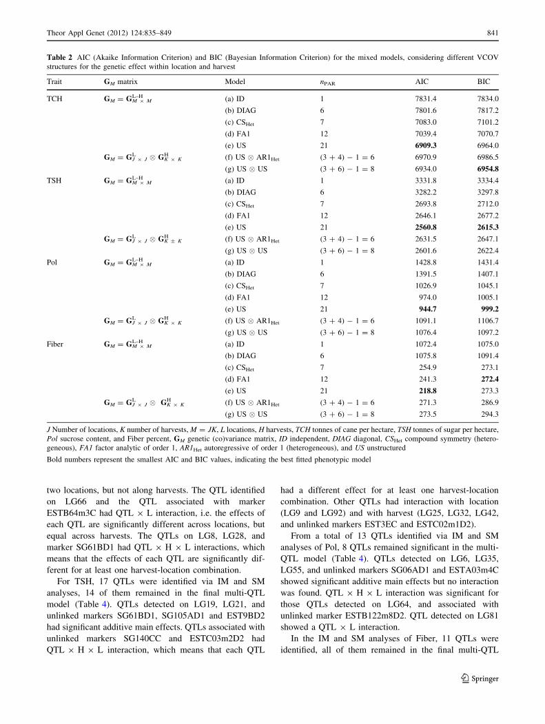
Multi-harvest-location phenotypic analysis

While the selected VCOV models for the G matrix based

on AIC and BIC criteria (Table 2) coincided for TSH (both

criteria selected model e) and so for Pol (both criteria

selected model e), different VCOVs were selected for the

G matrix for TCH (models e and g) as well as for Fiber

(models e and d). However, the differences of AIC values

from first and second best models were greater than the

respective BIC differences for both TCH and Fiber.

Therefore, we decided to use VCOVs selected via AIC

criterion, which in this study led to model (e) for all traits.

Although model (e) requires estimation of a larger number

of parameters, it had the smallest AIC throughout traits.

For the non-genetic residual effects, the model combining

an unstructured matrix RHK�K for harvests and a diagonal

matrix RLJ�J for locations had the smallest AIC when

compared with simpler models, such as the model assum-

ing heterogeneity of non-genetic residual variances and

absence of correlation between harvest-location combina-

tions (DIAG). The selected RM matrix was included in the

final phenotypic model, taking into account the existence

of non-genetic residual correlations and heterogeneity of

non-genetic residual variances across harvests and

locations.

QTL analysis

The search for QTL via IM (see step I in QTL analysis of

‘‘Materials and methods’’) led to the identification of 29

putative QTLs, 9 for TCH, 9 for TSH, 5 for Pol, and 6 for

Fiber (Fig. 2). Each QTL was located on a different LG.

Twenty-six marker-QTL associations were found in the

SM analyses (see step II in QTL analysis ‘‘Materials and

methods’’): five for TCH, eight for TSH, eight for Pol, and

five for Fiber (Online Supplementary Material). Genomic

positions and single markers significantly associated with

putative QTL in the IM and SM analyses were included in

the multi-QTL model for the estimation of QTL main

effects and QTL harvest-location-specific effects.

IM and SM analyses identified 14 QTLs for TCH, 13 of

which after been included in a multi-QTL model and been

tested (see steps III and IV of QTL analysis ‘‘Materials and

methods’’) remained in the final multi-QTL model

(Table 3). The QTLs identified on LG9 and LG19 had

significant additive main effect. QTLs detected on LG25,

LG32, LG72, LG92, and unlinked markers EST3EC and

ESTC81m3C had significant QTL 9 H interaction, indi-

cating that these QTLs showed the same behavior along the

840 Theor Appl Genet (2012) 124:835–849

123

two locations, but not along harvests. The QTL identified

on LG66 and the QTL associated with marker

ESTB64m3C had QTL 9 L interaction, i.e. the effects of

each QTL are significantly different across locations, but

equal across harvests. The QTLs on LG8, LG28, and

marker SG61BD1 had QTL 9 H 9 L interactions, which

means that the effects of each QTL are significantly dif-

ferent for at least one harvest-location combination.

For TSH, 17 QTLs were identified via IM and SM

analyses, 14 of them remained in the final multi-QTL

model (Table 4). QTLs detected on LG19, LG21, and

unlinked markers SG61BD1, SG105AD1 and EST9BD2

had significant additive main effects. QTLs associated with

unlinked markers SG140CC and ESTC03m2D2 had

QTL 9 H 9 L interaction, which means that each QTL

had a different effect for at least one harvest-location

combination. Other QTLs had interaction with location

(LG9 and LG92) and with harvest (LG25, LG32, LG42,

and unlinked markers EST3EC and ESTC02m1D2).

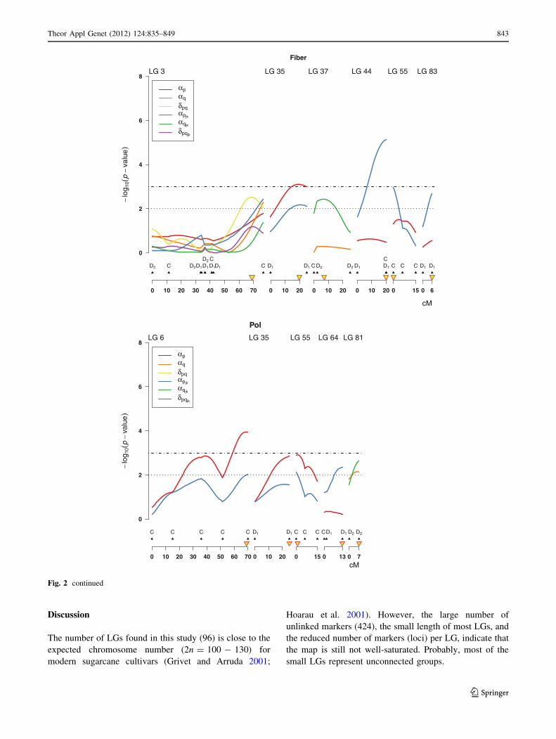
From a total of 13 QTLs identified via IM and SM

analyses of Pol, 8 QTLs remained significant in the multi-

QTL model (Table 4). QTLs detected on LG6, LG35,

LG55, and unlinked markers SG06AD1 and ESTA03m4C

showed significant additive main effects but no interaction

was found. QTL 9 H 9 L interaction was significant for

those QTLs detected on LG64, and associated with

unlinked marker ESTB122m8D2. QTL detected on LG81

showed a QTL 9 L interaction.

In the IM and SM analyses of Fiber, 11 QTLs were

identified, all of them remained in the final multi-QTL

Table 2 AIC (Akaike Information Criterion) and BIC (Bayesian Information Criterion) for the mixed models, considering different VCOV

structures for the genetic effect within location and harvest

Trait GM matrix Model nPAR AIC BIC

TCH GM = GM 9 ML–H (a) ID 1 7831.4 7834.0

(b) DIAG 6 7801.6 7817.2

(c) CSHet 7 7083.0 7101.2

(d) FA1 12 7039.4 7070.7

(e) US 21 6909.3 6964.0

GM = GJ 9 JL � GK 9 K

H (f) US � AR1Het (3 ? 4) - 1 = 6 6970.9 6986.5

(g) US � US (3 ? 6) - 1 = 8 6934.0 6954.8

TSH GM = GM 9 ML–H (a) ID 1 3331.8 3334.4

(b) DIAG 6 3282.2 3297.8

(c) CSHet 7 2693.8 2712.0

(d) FA1 12 2646.1 2677.2

(e) US 21 2560.8 2615.3

GM = GJ 9 JL � GK ± K

H (f) US � AR1Het (3 ? 4) - 1 = 6 2631.5 2647.1

(g) US � US (3 ? 6) - 1 = 8 2601.6 2622.4

Pol GM = GM 9 ML–H (a) ID 1 1428.8 1431.4

(b) DIAG 6 1391.5 1407.1

(c) CSHet 7 1026.9 1045.1

(d) FA1 12 974.0 1005.1

(e) US 21 944.7 999.2

GM = GJ 9 JL � GK 9 K

H (f) US � AR1Het (3 ? 4) - 1 = 6 1091.1 1106.7

(g) US � US (3 ? 6) - 1 = 8 1076.4 1097.2

Fiber GM = GM 9 ML–H (a) ID 1 1072.4 1075.0

(b) DIAG 6 1075.8 1091.4

(c) CSHet 7 254.9 273.1

(d) FA1 12 241.3 272.4

(e) US 21 218.8 273.3

GM = GJ 9 JL � GK 9 K

H (f) US � AR1Het (3 ? 4) - 1 = 6 271.3 286.9

(g) US � US (3 ? 6) - 1 = 8 273.5 294.3

J Number of locations, K number of harvests, M = JK, L locations, H harvests, TCH tonnes of cane per hectare, TSH tonnes of sugar per hectare,

Pol sucrose content, and Fiber percent, GM genetic (co)variance matrix, ID independent, DIAG diagonal, CSHet compound symmetry (hetero-

geneous), FA1 factor analytic of order 1, AR1Het autoregressive of order 1 (heterogeneous), and US unstructured

Bold numbers represent the smallest AIC and BIC values, indicating the best fitted phenotypic model

Theor Appl Genet (2012) 124:835–849 841

123

model (Table 4). A QTL with dominance effect was

identified on LG3. QTLs detected on LG35, and unlinked

markers SG25BC and ESTC110m2C showed significant

main effects but no interaction was found. QTL 9 L

interaction was detected for unlinked marker SG99DC,

which means that each QTL had different effects across

locations, but not across harvests. Other QTLs identified on

LG37, LG44, LG55, LG83, and unlinked markers

ESTA32m1C and ESTB153m1D2 showed QTL 9 H 9 L

interaction.

0

2

4

6

8

TCH−

log 1

0(p

−va

lue)

0 10 20 30 40 50 60

LG 8

0 10 20 30 40 50 60

LG 9

0 10 20 30 40

LG 19

0 10 20 30

LG 25

0 10 20

LG 28

0 10 20

LG 32

0 13

LG 66

0 10

LG 72

0

LG 92

cM

4

D2 D2 D2 D2 D2 D1 D1 D1 D1 D1 D1 D2 D2 D2 D2C D2 C D1 C C C C D2 C C D2 D2 C C D1 D1 D2D2

αpαq

δpqαpjk

αqjk

δpqjk

0

2

4

6

8

TSH

−lo

g 10(

p−

valu

e)

0 10 20 30 40 50 60

LG 8

0 10 20 30 40

LG 19

0 10 20 30 40

LG 21

0 10 20 30

LG 25

0 10 20

LG 32

0 10 20

LG 42

0 17

LG 50

0 13

LG 66

0

LG 92

cM

4

D2 D2 D2 D2 D2 D2 D2 D2 D2C D2 D1 D1 D1 C D1 C D2 C C D2 D2 D1 D1 CC C C C D2D2

αpαq

δpqαpjk

αqjk

δpqjk

Fig. 2 Interval mapping search of putative QTL (red- and yellow-

inverted triangles) associated with cane yield (tonnes of cane per

hectare, TCH), sugar yield (tonnes of sugar per hectare, TSH), fiber

content, and sucrose content (Pol) using a mixed model with

unstructured GM matrix (model e; Table 2). Two different situations

were considered: (1) using only main effects, model 5 (ap and aq:

additive effects on parents P and Q, respectively; and dpq:

dominance); (2) using genetic effects specifically for each harvest-

location combination, through model 4 (apjk; aqjk

and dpqjk). Not all

effects were estimated for all genomic positions due to lack of

information conveyed by SDMs (see ‘‘Materials and methods’’);

black triangles marker positions, dot-dashed line -log10(0.001) and

dotted line -log10(0.01). Marker types D1 and D2 segregate for parent

P and Q, respectively, while marker C segregates for both parents

842 Theor Appl Genet (2012) 124:835–849

123

Discussion

The number of LGs found in this study (96) is close to the

expected chromosome number (2n = 100 - 130) for

modern sugarcane cultivars (Grivet and Arruda 2001;

Hoarau et al. 2001). However, the large number of

unlinked markers (424), the small length of most LGs, and

the reduced number of markers (loci) per LG, indicate that

the map is still not well-saturated. Probably, most of the

small LGs represent unconnected groups.

0

2

4

6

8

−lo

g 10(

p−

valu

e)

0 10 20 30 40 50 60 70

LG 3

0 10 20

LG 35

0 10 20

LG 37

0 10 20

LG 44

0 15

LG 55

0 6

LG 83

cM

D2 C CD2 C D2D1D1 D1D1 C D1 D1 C D2 D2 D1 D1 C C C D1 D1

αpαq

δpqαpjk

αqjk

δpqjk

0

2

4

6

8

Pol

−lo

g 10(

p−

valu

e)

0 10 20 30 40 50 60 70

LG 6

0 10 20

LG 35

0 15

LG 55

0 13

LG 64

0 7

LG 81

cM

C C C C C D1 D1 C C C CD1 D1 D2 D2

αpαq

δpqαpjk

αqjk

δpqjk

Fiber

Fig. 2 continued

Theor Appl Genet (2012) 124:835–849 843

123

On one hand, usually only SDMs are used for linkage

map estimation (Ming et al. 1998), thus gaps in sugarcane

maps are commonly expected due to the exclusion of

multiple dose markers, such as, duplex of monoparental

origin, triplex or higher multiplex markers. Therefore,

linkage maps based solely on SDMs are not optimal for

QTL mapping and lower statistical power is possibly

expected. On the other hand, we estimated an integrated

map via multipoint likelihood (OneMap, Margarido et al.

2007). Our integrated map had higher likelihood than other

single-dose-based maps estimated from our population

(Garcia et al. 2006; Oliveira et al. 2007). Since multipoint

likelihood can put together in the same LG markers with

3:1 and 1:1 segregation patterns, the resulting integrated

map is more saturated and conveys higher representation of

the biparental genetic polymorphism than its counter part

double pseudo-testcross maps, hence, higher statistical

power is expected in the QTL analysis. Moreover, the use

of an integrated map allowed us to estimate additive effects

in each parent (ap and aq) and dominance effect (dpq),

which to the best of our knowledge is being proposed for

the first time to map QTL in sugarcane.

In spite of the interspecific origin of modern commercial

sugarcane cultivars with genome composition of about

70–80% of Saccharum officinarum, 10–20% of S. sponta-

neum and 5–17% of recombinant chromosomes (D’Hont

et al. 1996; Grivet and Arruda 2001; Jannoo et al. 2004;

D’Hont 2005; Piperidis et al. 2010), and the high level of

polyploidy and aneuploidy, the number of putative HGs

identified (11) are in close agreement with the expected

number for sugarcane, as the basic number of chromo-

somes (x) of the genus Saccharum can range from x = 8 to

x = 10 (D’Hont et al. 1998; Irvine 1999; Grivet and Arr-

uda 2001; Piperidis et al. 2010).

Despite varietal selection of sugarcane based on quan-

titative traits is usually done with measurements taken from

series of field trials in multiple locations and multiple

harvests, fitting alternative VCOV structures for modeling

genetic effect across locations and harvests is seldom

pursued (Smith et al. 2007). Mixed models were used in

this study due to their flexibility to model VCOV structures

that appears when repeated measures are taken across

locations and harvests. In the mixed model analyses,

genotypes in the progeny were assumed to be random

because the main interest is in the genetic variation of

genotypes in the progeny rather than the genotypes them-

selves. The effects of location (L) and harvest (H) were

taken as fixed. Models that exploit the direct product of

(co)variance matrices (models f–g) have fewer parameters,

and therefore, we would expect them to show smaller AIC

values. However, the unstructured VCOV matrix (model

e), modeling specific genetic variances or covariances for

each environment, showed smaller AIC values throughout

all traits, despite its larger number of parameters. Although

it is well-documented in the literature that AIC tends to

select models with more parameters as compared with BIC,

the choice of unstructured VCOV model shows some

evidence for the presence of heterogeneity of variances and

covariances across different harvest-location combinations

(Table 5).

Table 3 QTL effects estimated with the multi-QTL mixed model and the average standard error of all pairwise differences ( �sedif )

Trait LG (effect) Markers Position Location–harvest ( �sedif )

(cM) 1–1 1–2 1–3 2–1 2–2 2–3

TCH 8 (aqjk) EST2DD2/SG04AD1 0.0 1.61 0.68 0.83 -2.32 -0.11 0.82 (1.26)

9 (ap) ESTB27m2D1/ESTC123m4D1 42.0 3.81 3.81 3.81 3.81 3.81 3.81 (1.26)a

19 (aq) ESTB157m4D2/ESTB157m1D2 13.0 4.20 4.20 4.20 4.20 4.20 4.20 (1.26)a

25 (aqk) EST1CC/ESTC47m3D1 3.0 -1.82 -4.10 -5.86 -1.82 -4.10 -5.86 (1.20)

28 (apjk) SG11FC/ESTA15m3C 13.0 2.50 -0.20 2.58 0.86 0.82 -1.06 (2.03)

32 (aqk) ESTA63m3D2/ESTA48m2D2 22.0 -2.14 -2.98 -1.78 -2.14 -2.98 -1.78 (0.69)

66 (apj) ESTA68m1C/ESTC129m5C 12.7 -7.40 -7.40 -7.40 -1.62 -1.62 -1.62 (1.57)

72 (apk) ESTA54m3D1/ESTB94m6D1 3.0 1.42 4.11 3.94 1.42 4.11 3.94 (0.72)

92 (aqk) ESTB65m1D2/ESTC44m1D2 4.0 1.85 1.67 0.16 1.85 1.67 0.16 (0.69)

NL (apjk) SG61BD1 4.97 3.53 2.72 2.32 3.43 3.33 (1.25)

NL (apk) EST3EC 1.81 0.88 -0.71 1.81 0.88 -0.71 (0.86)

NL (apj) ESTB64m3C 7.02 7.02 7.02 1.36 1.36 1.36 (1.63)

NL (apk) ESTC81m3C 1.86 5.11 5.84 1.86 5.11 5.84 (0.84)

NL Not-linked markers, TCH tonnes of cane per hectare, ap and aq are additive main effects on parents P and Q, respectively, while dpq is

dominance; apjk; aqjk

and dpqjkare the harvest-location-specific effects

a Standard error

844 Theor Appl Genet (2012) 124:835–849

123

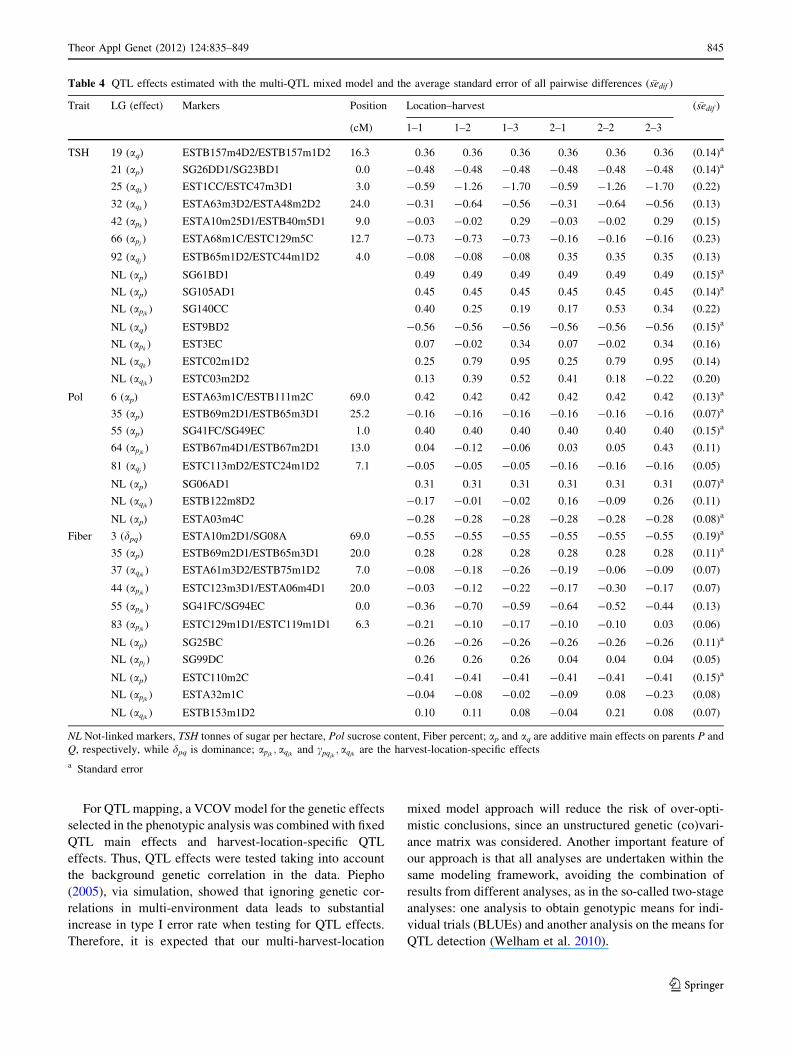
For QTL mapping, a VCOV model for the genetic effects

selected in the phenotypic analysis was combined with fixed

QTL main effects and harvest-location-specific QTL

effects. Thus, QTL effects were tested taking into account

the background genetic correlation in the data. Piepho

(2005), via simulation, showed that ignoring genetic cor-

relations in multi-environment data leads to substantial

increase in type I error rate when testing for QTL effects.

Therefore, it is expected that our multi-harvest-location

mixed model approach will reduce the risk of over-opti-

mistic conclusions, since an unstructured genetic (co)vari-

ance matrix was considered. Another important feature of

our approach is that all analyses are undertaken within the

same modeling framework, avoiding the combination of

results from different analyses, as in the so-called two-stage

analyses: one analysis to obtain genotypic means for indi-

vidual trials (BLUEs) and another analysis on the means for

QTL detection (Welham et al. 2010).

Table 4 QTL effects estimated with the multi-QTL mixed model and the average standard error of all pairwise differences ( �sedif )

Trait LG (effect) Markers Position Location–harvest ( �sedif )

(cM) 1–1 1–2 1–3 2–1 2–2 2–3

TSH 19 (aq) ESTB157m4D2/ESTB157m1D2 16.3 0.36 0.36 0.36 0.36 0.36 0.36 (0.14)a

21 (ap) SG26DD1/SG23BD1 0.0 -0.48 -0.48 -0.48 -0.48 -0.48 -0.48 (0.14)a

25 (aqk) EST1CC/ESTC47m3D1 3.0 -0.59 -1.26 -1.70 -0.59 -1.26 -1.70 (0.22)

32 (aqk) ESTA63m3D2/ESTA48m2D2 24.0 -0.31 -0.64 -0.56 -0.31 -0.64 -0.56 (0.13)

42 (apk) ESTA10m25D1/ESTB40m5D1 9.0 -0.03 -0.02 0.29 -0.03 -0.02 0.29 (0.15)

66 (apj) ESTA68m1C/ESTC129m5C 12.7 -0.73 -0.73 -0.73 -0.16 -0.16 -0.16 (0.23)

92 (aqj) ESTB65m1D2/ESTC44m1D2 4.0 -0.08 -0.08 -0.08 0.35 0.35 0.35 (0.13)

NL (ap) SG61BD1 0.49 0.49 0.49 0.49 0.49 0.49 (0.15)a

NL (ap) SG105AD1 0.45 0.45 0.45 0.45 0.45 0.45 (0.14)a

NL (apjk) SG140CC 0.40 0.25 0.19 0.17 0.53 0.34 (0.22)

NL (aq) EST9BD2 -0.56 -0.56 -0.56 -0.56 -0.56 -0.56 (0.15)a

NL (apk) EST3EC 0.07 -0.02 0.34 0.07 -0.02 0.34 (0.16)

NL (aqk) ESTC02m1D2 0.25 0.79 0.95 0.25 0.79 0.95 (0.14)

NL (aqjk) ESTC03m2D2 0.13 0.39 0.52 0.41 0.18 -0.22 (0.20)

Pol 6 (ap) ESTA63m1C/ESTB111m2C 69.0 0.42 0.42 0.42 0.42 0.42 0.42 (0.13)a

35 (ap) ESTB69m2D1/ESTB65m3D1 25.2 -0.16 -0.16 -0.16 -0.16 -0.16 -0.16 (0.07)a

55 (ap) SG41FC/SG49EC 1.0 0.40 0.40 0.40 0.40 0.40 0.40 (0.15)a

64 (apjk) ESTB67m4D1/ESTB67m2D1 13.0 0.04 -0.12 -0.06 0.03 0.05 0.43 (0.11)

81 (aqj) ESTC113mD2/ESTC24m1D2 7.1 -0.05 -0.05 -0.05 -0.16 -0.16 -0.16 (0.05)

NL (ap) SG06AD1 0.31 0.31 0.31 0.31 0.31 0.31 (0.07)a

NL (aqjk) ESTB122m8D2 -0.17 -0.01 -0.02 0.16 -0.09 0.26 (0.11)

NL (ap) ESTA03m4C -0.28 -0.28 -0.28 -0.28 -0.28 -0.28 (0.08)a

Fiber 3 (dpq) ESTA10m2D1/SG08A 69.0 -0.55 -0.55 -0.55 -0.55 -0.55 -0.55 (0.19)a

35 (ap) ESTB69m2D1/ESTB65m3D1 20.0 0.28 0.28 0.28 0.28 0.28 0.28 (0.11)a

37 (aqjk) ESTA61m3D2/ESTB75m1D2 7.0 -0.08 -0.18 -0.26 -0.19 -0.06 -0.09 (0.07)

44 (apjk) ESTC123m3D1/ESTA06m4D1 20.0 -0.03 -0.12 -0.22 -0.17 -0.30 -0.17 (0.07)

55 (apjk) SG41FC/SG94EC 0.0 -0.36 -0.70 -0.59 -0.64 -0.52 -0.44 (0.13)

83 (apjk) ESTC129m1D1/ESTC119m1D1 6.3 -0.21 -0.10 -0.17 -0.10 -0.10 0.03 (0.06)

NL (ap) SG25BC -0.26 -0.26 -0.26 -0.26 -0.26 -0.26 (0.11)a

NL (apj) SG99DC 0.26 0.26 0.26 0.04 0.04 0.04 (0.05)

NL (ap) ESTC110m2C -0.41 -0.41 -0.41 -0.41 -0.41 -0.41 (0.15)a

NL (apjk) ESTA32m1C -0.04 -0.08 -0.02 -0.09 0.08 -0.23 (0.08)

NL (aqjk) ESTB153m1D2 0.10 0.11 0.08 -0.04 0.21 0.08 (0.07)

NL Not-linked markers, TSH tonnes of sugar per hectare, Pol sucrose content, Fiber percent; ap and aq are additive main effects on parents P and

Q, respectively, while dpq is dominance; apjk; aqjk

and cpqjk; aqjk

are the harvest-location-specific effects

a Standard error

Theor Appl Genet (2012) 124:835–849 845

123

Amongst all traits, many QTLs (65%) showed signifi-

cant interaction: QTL 9 H (24%), QTL 9 L (13%),

QTL 9 H 9 L (28%) interaction; and 17 QTLs (35%) had

stable effect across harvests and locations. The number of

detected interactions was greater for QTL 9 H than for

QTL 9 L, possibly because genotype by harvest (G 9 H)

interaction accounted for great part of the genotype by

environment interaction for each trait, and, moreover, there

was no significant genotype by location (G 9 L) interac-

tion for Pol and Fiber.

On one hand, QTL whose effects are not statistically

different across harvests and locations are important for

studies that seek to identify major genes controlling agro-

nomic traits, as the expression of these genes would not be

expected to change drastically across harvest-location

combinations. For example: QTLs identified on LG9 and

LG19 (TCH), LG19, LG21, unlinked markers SG61BD1,

SG105AD1 and EST9BD2 (TSH), LG6, LG35, LG55,

unlinked markers SG06AD1 and ESTA03m4C (Pol), LG3,

LG35, unlinked markers SG25BC and ESTC110m2C

(Fiber). It is worth mentioning that 62.5% of QTLs identi-

fied for Pol were stable across all harvest-location combi-

nations, corroborating the speculated fact raised by many

breeders that Pol has reached the plateau of adaptability and

stability. On the other hand, QTLs with stable effects across

harvests within locations (likewise, stable effects across

locations within harvests) are also important to identify

genes with similar expression across harvests (likewise,

across locations). For instance: QTLs located on LG66 and

unlinked marker ESTB64m3C (TCH), LG66 and LG92

(TSH), LG81 (Pol), and unlinked marker SG99DC (Fiber).

Not only QTL effect stability is important to applications,

but also its sign and magnitude, as for example in MAS. To

exemplify, QTLs on LG8 and LG28 of TCH changed signs

across some harvest-location combinations, and QTL on

LG25 had negative effect with increasing magnitude across

harvests, which is particularly interesting in sugarcane,

since yield decreases across harvests.

Assignment of LGs to HGs may help us to infer whether

QTLs mapped at distinct LGs, but in genomic regions that

share at least a common locus, are the same or not. For

example, while QTLs detected on LG8 and LG50 (TSH)

were assigned to HGIV, they were positioned far apart at

4.7 cM and 17.1 cM from their common locus ESTA47,

respectively. Therefore, we cannot infer that these genomic

regions share the same QTL. Likewise, although QTLs

detected on LG25 and LG28 (TCH), LG3 and LG35

(Fiber) belong to HGI and HGV, respectively, they are far

apart from their common locus ESTA15 (TCH), ESTB65

and ESTB69 (Fiber), hence, they represent different QTLs.

It is important to notice that the linkage map estimated in

this study is not well-saturated. Adding more markers to

the data may change the number, length and marker

ordering of LGs, therefore, possibly conveying more

information about whether QTLs mapped on LGs belong-

ing to an HG are the same or not.

Some QTLs of different traits were identified in com-

mon linkage groups or associated with common markers.

For example, both TCH and TSH had one QTL mapped on

each of the following LGs and unlinked markers: LG19,

LG25, LG32, LG66 and LG92, and markers SG61BD1,

EST3EC and ESTC03m2D2. As all the common QTLs

were close by, it is possible that they are pleiotropic QTLs.

It was expected that these traits would have some QTLs in

common, since they are strongly correlated. Both Pol and

Fiber had a QTL on LG35, possibly they are just one

pleiotropic QTL. In breeding programs, special attention

should be given to these two QTLs when simultaneous

improvement is aimed for Pol and Fiber, since the QTLs

had opposite signs on these traits. Moreover, the negative

correlation between Pol and Fiber is interesting to the

modern trend of industrial production of second-generation

(cellulosic) ethanol, which seeks for sugarcane varieties

specialized in biomass production with higher fiber

content.

We aimed to compare our multi-harvest-location mod-

eling strategy (mixed model) with other strategies of

modeling QTL 9 H 9 L interaction in sugarcane, but no

other study of this nature has been pursued, to the best of

our knowledge (Pastina et al. 2010). However, some

attempts to study QTL 9 H 9 L interaction have been

made via SM analyses of each harvest or harvest-location

combination (when available) separately, for each parent

through the pseudo-testcross strategy. Stability of QTLs

across environments were inferred based on their effect

sizes (Hoarau et al. 2002; Jordan et al. 2004; McIntyre

et al. 2005a, b; Reffay et al. 2005; Aitken et al. 2006,

2008; Al-Janabi et al. 2007; Piperidis et al. 2008). Never-

theless, none of these studies could be compared to ours

due to differences in the data. Therefore, IM was carried

out through R/qtl for each trait and harvest-location com-

bination separately (univariate QTL analyses, Online

Supplementary Material) to be compared with our mixed-

Table 5 Estimated genetic (co)variance matrix GM for TCH, using

model (e) for the multi-harvest-location phenotypic analysis

Location–

harvest

1–1 1–2 1–3 2–1 2–2 2–3

1–1 302.64 0.95 0.92 0.86 0.88 0.81

1–2 386.64 543.35 1.00 0.80 0.93 0.81

1–3 389.33 576.19 588.04 0.81 0.93 0.91

2–1 200.32 249.32 262.79 178.24 0.95 0.82

2–2 269.25 380.72 397.41 224.55 310.18 1.00

2–3 241.79 352.72 378.03 187.94 303.17 292.40

Genetic correlations are shown above the diagonal

846 Theor Appl Genet (2012) 124:835–849

123

model approach. Through this separate analyses it was

possible to identify only one putative QTL for TCH and

two for Pol. For TCH, the QTL was positioned on LG32,

which had a significant effect for harvests 1 and 2 in

location 1. For location 2 there were some evidences of

QTLs on LG32 with different effects across harvests,

however, the LOD values were smaller than the threshold

considered (LOD = 3). These QTL may correspond to the

QTL identified in the same LG using mixed model, which

showed unstable effect across harvests. For Pol, two dif-

ferent QTLs were identified, one on LG6 and other on

LG55, which were also identified in the mixed model

analysis. The QTLs identified on LG6 and LG55 had sig-

nificant effects for harvest 2 in location 1 and harvest 2 in

location 2, respectively, which do not agree with the mixed

model analysis, since stable effects were found across all

harvest-location combinations. Overall, while separate

analyses found only three QTLs, the mixed model analyses

found forty-six, clearly showing the overwhelming

advantage of the mixed model approach.

QTL mapping in sugarcane still presents several diffi-

culties, such as the use of only SDMs, low saturated

linkage maps, small sample size (ng), the occurrence of

collinearity between the additive genetic predictors esti-

mated for parents (as a consequence of the lack of infor-

mation conveyed by SDMs). The latter difficulty restricted

the estimation of dominance genetic predictor for only a

limited number of linkage groups (LG2, LG3, LG14,

LG18, LG37 and LG41). Thus, the fact that only one QTL

with dominance effect was found for Fiber is not neces-

sarily related to the genetic basis of this trait, but due to the

fact that we simply often could not estimate and test for it.

We are also aware that the small sample size used

(ng = 100) has reduced statistical power, but the focus of

our work was on the illustration of how to use a mixed-

model framework that takes into account heterogeneity of

genetic and non-genetic residual variances and covari-

ances. Despite these limitations, the present study provides

many contributions, such as, the identification of a con-

siderable number of QTLs for the evaluated traits, with

information about effect sizes, positions, stability of QTLs,

and presence of QTL 9 H, QTL 9 L, and QTL 9 H 9 L

interactions. Therefore, unveiling the genetic architecture

of sugarcane production and sucrose content, which are

complex traits. In addition, the statistical models used here

can be used in future QTL studies involving multiplex

markers in addition to SDMs.

Acknowledgments The authors want to thank the anonymous

reviewers for their suggestions, and Luciano da Costa e Silva to

carefully read and give suggestions for the final English version. This

research was supported by Conselho Nacional de Desenvolvimento

Cientıfico e Tecnologico (CNPq, grant 140680/2005-5 and

201409/2008-9) and Fundacao de Amparo a Pesquisa do Estado de

Sao Paulo (FAPESP, grant 2008/52197-4 and 2010/00083-5), both

from Brazil. It was also part of the researches of the Instituto Nacional

de Ciencia e Tecnologia do Bioetanol (granted by CNPq,

574002/2008-1, and FAPESP, 2008/57908-6) and of the PhD Thesis

of M.M. Pastina, presented at Escola Superior de Agricultura ‘‘Luiz

de Queiroz’’, Universidade de Sao Paulo. M.M. Pastina was working

under the supervision of F.A. van Eeuwijk at Biometris Department,

Plant Sciences Group, Wageningen University, from February/2009

to September/2009. A.A.F. Garcia and A.P. Souza are recipients of

research fellowship from CNPq.

Open Access This article is distributed under the terms of the

Creative Commons Attribution Noncommercial License which per-

mits any noncommercial use, distribution, and reproduction in any

medium, provided the original author(s) and source are credited.

References

Aitken KS, Jackson PA, McIntyre CL (2006) Quantitative trait loci

identified for sugar related traits in a sugarcane (Saccharum spp.)

cultivar x Saccharum officinarum population. Theor Appl Genet

112:1306–1317

Aitken KS, Hermann S, Karno K, Bonnett GD, McIntyre LC, Jackson

PA (2008) Genetic control of yield related stalk traits in

sugarcane. Theor Appl Genet 117:1191–1203

Akaike H (1974) A new look at the statistical model identification.

IEEE Trans Automat Contr AC 19:716–723

Al-janabi SM, Honeycutt RJ, Mcclelland M, Sobral BWS (1993) A

genetic linkage map of Saccharum spontaneum L. ’SES 208’.

Genetics 134:1249–1260

Al-Janabi SM, Parmessur Y, Kross H, Dhayan S, Saumtally S,

Ramdoyal K, Autrey LJC, Dookun-Saumtally A (2007) Identi-

fication of a major quantitative trait locus (QTL) for yellow spot

(Mycovellosiella koepkei) disease resistance in sugarcane. Mol

Breed 19:1–14

Boer MP, Wright D, Feng L, Podlich DW, Luo L, Cooper M, van

Eeuwijk FA (2007) A mixed-model quantitative trait loci (QTL)

analysis for multiple-environment trial data using environmental

covariables for QTL-by-environment interactions, with an

example in maize. Genetics 177:1801–1813

Broman KW, Wu H, Sen S, Churchill GA (2003) R/qtl: QTL mapping

in experimental crosses. Bioinformatics 19:889–890

Carlier JD, Reis A, Duval MF, Coppens D’Eeckenbrugge G, Leitao

JM (2004) Genetic maps of RAPD, AFLP and ISSR markers in

Ananas bracteatus and A. comosus using the pseudo-testcross

strategy. Plant Breed 123:186–192

Cavalcanti JJV, Wilkinson MJ (2007) The first genetic maps of

cashew (Anacardium occidentale L.). Euphytica 157:131–143

Chapman SC (2008) Use of crop models to understand genotype by

environment interactions for drought in real-world and simulated

plant breeding trials. Euphytica 161:195–208

Chen C, Bowman KD, Choi YA, Dang PM, Rao MN, Huang S,

Soneji JR, McCollum TG, Gmitter FG (2008) EST-SSR genetic

maps for Citrus sinensis and Poncirus trifoliata. Tree Genetics

Genomes 4:1–10

Cullis B, Gogel B, Verbyla A, Thompson R (1998) Spatial analysis of

multi-environment early generation variety trials. Biometrics

54(1):1–18

Daugrois JH, Grivet L, Roques D, Hoarau JY, Lombard H,

Glaszmann JC, D’Hont A (1996) A putative major gene for

rust resistance linked with a RFLP marker in sugarcane cultivar

’R570’. Theor Appl Genet 92:1059–1064

Theor Appl Genet (2012) 124:835–849 847

123

da Silva JA, Bressiani JA (2005) Sucrose synthase molecular marker

associated with sugar content in elite sugarcane progeny. Genet

Mol Biol 28(2):294–298

Denis JB, Piepho HP, van Eeuwijk FA (1997) Modelling expectation

and variance for genotype by environment data. Heredity

79:162–171

D’Hont A (2005) Unravelling the genome structure of polyploids

using FISH and GISH; examples in sugarcane and banana.

Cytogenet Genome Res 109:27–33

D’Hont A, Grivet L, Feldman P, Rao S, Berding N, Glaszmann JC

(1996) Characterisation of the double genome structure of

modern sugarcane cultivares (Saccharum spp.) by molecular

cytogenetics. Mol Gen Genet 250:405–413

D’Hont A, Ison D, Alix K, Roux C, Glaszmann JC (1998)

Determination of basic chromosome numbers in the genus

Saccharum by physical mapping of ribosomal RNA genes.

Genome 41:221–225

Eckermann PJ, Verbyla AP, Cullis BR, Thompson R (2001) The

abalysis of quantitative traits in wheat mapping populations.

Aust J Agric Res 52:1195–1206

Garcia AAF, Kido EA, Meza AN, Silva JAGD, Souza AP, Pinto LR,

Pastina MM, Leite CS, da Silva JAG, Ulian EC, Figueira A,

Souza HMB (2006) Development of an integrated genetic map

of a sugarcane (Saccharum spp.) commercial cross, based on a

maximum-likelihood approach for estimation of linkage and

linkage phases. Theor Appl Genet 112:298–314

Gazaffi R (2009) Desenvolvimento de modelo genetico estatıstico

para mapeamento de QTLs em progenie de irmaos completos,

com aplicacao em cana-de-acucar. PhD Thesis, Escola Superior

de Agricultura Luiz de Queiroz, Universidade de Sao Paulo,

Brazil

Gogel BJ, Cullis BR, Verbyla AP (1995) REML estimation of

multiplicative effects in multi-environment variety trials. Bio-

metrics 51(2):744–749

Grattapaglia D, Sederoff R (1994) Genetic linkage maps of Eucalyp-

tus grandis and Eucalyptus urophylla using a pseudo-testcross:

mapping strategy and RAPD markers. Genetics 137:1121–1137

Grivet L, Arruda P (2001) Sugarcane genomics: depicting the

complex genome of an important tropical crop. Curr Opin Plant

Biol 5:122–127

Haley CS, Knott SA (1992) A simple regression method for mapping

quantitative trait loci in line crosses using flanking markers.

Heredity 69:315–324

Haley CS, Knott SA, Elsen JM (1994) Mapping quantitative trait loci

in crosses between outbred lines using least squares. Genetics

136:1195–1207

Heinz DJ, Tew TL (1987) Hybridization procedures. In: Heinz DJ

(eds) Sugarcane Improvement through Breeding, Elsevier,

Amsterdam, pp 313–342

Hoarau JY, Offmann B, D’Hont A, Risterucci AM, Roques D,

Glaszmann JC, Grivet L (2001) Genetic dissection of a modern

sugarcane cultivar (Saccharum spp.). I. Genome mapping with

AFLP markers. Theor Appl Genet 103:84–97

Hoarau JY, Grivet L, Offmann B, Raboin LM, Diorflar JP, Payet J,

Hellmann M, D’Hont A, Glaszmann JC (2002) Genetic dissec-

tion of a modern sugarcane cultivar (Saccharum spp.). II.

Detection of QTLs for yield components. Theor Appl Genet

105:1027–1037

Hu Z, Xu S (2009) Proc qtl—a sas procedure for mapping quantitative

trait loci. Int J Plant Genomics. doi:10.1155/2009/141234

Irvine JE (1999) Saccharum species as horticultural classes. Theor

Appl Genet 98:186–194

Jannoo N, Grivet L, David J, D’Hont A, Glaszmann JC (2004)

Differential chromosome pairing affinities at meiosis in poly-

ploid sugarcane revealed by molecular markers. Heredity

93:460–467

Jordan DR, Casu RE, Besse P, Carroll BC, Berding N, McIntyre CL

(2004) Markers associated with stalk number and suckering in

sugarcane colocate with tillering and rhizomatousness QTLs in

sorghum. Genome 47:988–993

Knott SA, Haley CS (1992) Maximum likelihood mapping of

quantitative trait loci using full-sib families. Genetics

132:1211–1222

Knott SA, Neale DB, Sewell MM, Haley CS (1997) Multiple marker

mapping of quantitative trait loci in an outbred pedigree of

loblolly pine. Theor Appl Genet 94:810–820

Kosambi DD (1944) The estimation of map distances from recom-

bination values. Annu Eugene 12:172–175

Lander E, Botstein D (1989) Mapping Mendelian factors underlying

quantitative traits using RFLP linkage maps. Genetics

121:185–199

Lander E, Green P, Abrahamson J, Barlow A, Daley M, Lincoln S,Newburg L (1987) MAPMAKER: an interactive computer

package for constructing primary genetic linkage maps of

experimental and natural populations. Genomics 1:174–181

Lin M, Lou X, Chang M, Wu R (2003) A general statistical

framework for mapping quantitative trait loci in nonmodel

systems: issue for characterizing linkage phases. Genetics

165:901–913

Lynch M, Walsh B (1998) Genetics and analysis of quantitative traits.

Sinauer Associates, Sunderland

Malosetti M, Voltas J, Romagosa I, Ullrich SE, van Eeuwijk FA (2004)

Mixed models including environmental covariables for studying

QTL by environment interaction. Euphytica 137:139–145

Malosetti M, Ribaut JM, Vargas M, Crossa J, van Eeuwijk FA (2008)

A multi-trait multi-environment QTL mixed model with an

application to drought and nitrogen stress trials in maize (Zeamays L.). Euphytica 161:241–257

Margarido GRA, Souza AP, Garcia AAF (2007) OneMap: software

for genetic mapping in outcrossing species. Hereditas 144:78–79

Martınez O, Curnow RN (1992) Estimating the locations and the sizes

of the effects of quantitative trait loci using flanking markers.

Theor Appl Genet 85:480–488

Mathews KL, Malosetti M, Chapman S, McIntyre L, Reynolds M,

Shorter R, van Eeuwijk F (2008) Multi-environment QTL mixed

models for drought stress adaptation in wheat. Theor Appl Genet

117:1077–1091

McIntyre C, Jackson M, Cordeiro G, Amouyal O, Hermann S, Aitken

K, Eliott F, Henry R, Casu R, Bonnett G (2006) The

identification and characterisation of alleles of sucrose phosphate

synthase gene family III in sugarcane. Mol Breed 18:39–50

McIntyre CL, Whan VA, Croft B, Magarey R, Smith GR (2005)

Identification and validation of molecular markers associated

with Pachymetra root rot and brown rust resistance in sugarcane

using map- and association-based approaches. Mol Breed

16:151–161

McIntyre CL, Casu RE, Drenth J, Knight D, Whan VA, Croft BJ,

Jordan DR, Manners JM (2005) Resistance gene analogues in

sugarcane and sorghum and their association with quantitative

trait loci for rust resistance. Genome 48:391–400

Ming R, Liu SC, Lin YR, da Silva J, Wilson W, Braga D, van Deynze

A, Wenslaff TF, Wu KK, Moore PH, Burnquist W, Sorrells ME,

Irvine JE, Paterson AH (1998) Detailed alignment of saccharum

and sorghum chromosomes: comparative organization of closely

related diploid and polyploid genomes. Genetics 150:1663–1682

Ming R, Liu SC, Moore PH, Irvine JE, Paterson AH (2001) QTL

analysis in a complex autopolyploid: genetic control of sugar

content in sugarcane. Genome Res 11:2075–2084

Ming R, Wang W, Draye X, Moore H, Irvine E, Paterson H (2002)

Molecular dissection of complex traits in autopolyploids:

mapping QTLs affecting sugar yield and related traits in

sugarcane. Theor Appl Genet 105:332–345

848 Theor Appl Genet (2012) 124:835–849

123

Ming R, Del Monte TA, Hernandez E, Moore PH, Irvine JE, Paterson

AH (2002) Comparative analysis of QTLs affecting plant height

and flowering among closely-related diploid and polyploid

genomes. Genome 45:794–803

Okada M, Lanzatella C, Saha MC, Bouton J, Wu R, Tobias CM

(2010) Complete switchgrass genetic maps reveal subgenome

collinearity, preferential pairing and multilocus interactions.

Genetics 185:745–760

Oliveira KM, Pinto LR, Marconi TG, Margarido GRA, Pastina MM,

Teixeira LHM, Figueira AV, Ulian EC, Garcia AAF, Souza AP

(2007) Functional integrated genetic linkage map based on EST-

markers for a sugarcane (Saccharum spp.) commercial cross.

Mol Breed 20:189–208

Oman SD (1991) Multiplicative effects in mixed model analysis of

variance. Biometrika 78(4):729–739

Pastina MM, Pinto LR, Oliveira KM, Souza AP, Garcia AAF (2010)

Molecular mapping of complex traits. In: Henry R, Kole C (eds)

Genetics, genomics and breeding of sugarcane, Science Pub-

lishers, Enfield, pp 117–148

Payne RW, Murray DA, Harding SA, Baird DB, Soutar DM (2009)

GenStat for Windows (12th Edition) Introduction. VSN Inter-

national, Hemel Hempstead

Piepho HP (1997) Analyzing genotype-environment data by mixed

models with multiplicative terms. Biometrics 53(2):761–766

Piepho HP (2000) A mixed-model approach to mapping quantitative

trait loci in barley on the basis of multiple environment data.

Genetics 156:2043–2050

Piepho HP (2005) Statistical tests for QTL and QTL-by-environment

effects in segregating populations derived from line crosses.

Theor Appl Genet 110:561–566

Pinto LR, Garcia AAF, Pastina MM, Teixeira LHM, Bressiani JA,

Ulian EC, Bidoia MAP, Souza AP (2010) Analysis of genomic

and functional RFLP derived markers associated with sucrose

content, fiber and yield QTLs in a sugarcane (Saccharum spp.)

commercial cross. Euphytica 172:313–327

Piperidis N, Jackson PA, D’Hont A, Besse P, Hoarau JY, Courtois B,

Aitken KS, McIntyre CL (2008) Comparative genetics in

sugarcane enables structured map enhancement and validation

of marker-trait associations. Mol Breed 21:233–247

Piperidis N, Piperidis G, D’Hont A (2010) Molecular cytogenetics. In:

Henry R, Kole C (eds) Genetics, genomics and breeding of

sugarcane, Science Publishers, Enfield, pp 9–18

Porceddu A, Albertini E, Barcaccia G, Falistocco E, Falcinelli M

(2002) Linkage mapping in apomictic and sexual Kentucky

bluegrass (Poa pratensis L.) genotypes using a two way pseudo-

testcross strategy based on AFLP and SAMPL markers. Theor

Appl Genet 104:273–280

Raboin LM, Oliveira KM, Raboin LM, Lecunff L, Telismart H,

Roques D, Butterfield M, Hoarau JY, D’Hont A (2006) Genetic

mapping in sugarcane, a high polyploid, using bi-parental

progeny: identification of a gene controlling stalk colour and a

new rust resistance gene. Theor Appl Genet 112:1382–1391

Reffay N, Jackson PA, Aitken KS, Hoarau JY, D’Hont A, Besse P,

McIntyre CL (2005) Characterisation of genome regions

incorporated from an important wild relative into Australian

sugarcane. Mol Breed 15:367–381

Ripol MI, Churchill GA, da Silva JAG, Sorrells M (1999) Statistical

aspects of genetic mapping in autopolyploids. Gene 235:31–41

Schafer-Pregl R, Salamini F, Gebhardt C (1996) Models for mapping

quantitative trait loci (QTL) in progeny of non-inbred parents

and their behaviour in presence of distorted segregation rations.

Genet Res 67:43–54

Schwarz G (1978) Estimating the dimension of a model. Ann Stat

6:461–464

Shepherd M, Cross M, Dieters MJ, Henry R (2003) Genetic maps for

Pinus elliottii var hondurensis using AFLP and microsatellite

markers. Theor Appl Genet 106:1409–1419

Sillanpaa M, Arjas E (1999) Bayesian mapping of multiple quanti-

tative trait loci from incomplete outbred offspring data. Genetics

151:1605–1619

Sills GR, Bridges W, Al-Janabi SM, Sobral BWS (1995) Genetic

analysis of agronomic traits in a cross between sugarcane

(Saccharum officinarum L.) and its presumed progenitor (S.robustum Brandes & Jesw. ex Grassl). Mol Breed 1:355–363

Smith A, Cullis B, Thompson R (2001) Analyzing variety by

environment data using multiplicative mixed models and

adjustments for spatial field trend. Biometrics 57(4):1138–1147

Smith AB, Stringer JK, Wei X, Cullis BR (2007) Varietal selection

for perennial crops where data relate to multiple harvests from a

series of field trials. Euphytica 157:253–266

Verbeke G, Molenberghs G (2000) Linear mixed models for

longitudinal data. Spinger, New York

van Eeuwijk FA, Malosetti M, Yin X, Struik PC, Stam P (2005)

Statistical models for genotype by environment data: from

conventional ANOVA models to eco-physiological QTL models.

Aust J Agric Res 56:883–894

van Eeuwijk FA, Malosetti M, Boer MP (2007) Modelling the genetic

basis of response curves underlying genotype 9 environment

interaction. In: Spiertz JHJ, Struik PC, van Laar HH (ed) Scale

and complexity in plant systems research: gene–plant–crop

relations. Springer, Dordrecht, pp 115–126

Verbyla A, Eckerman PJ, Thompson R, Cullis B (2003) The analysis

of quantitative trait loci in multi-environment trials using a

multiplicative mixed model. Aust J Agric Res 54:1395–1408

Welham S, Gogel B, Smith A, Thompson R, Cullis B (2010) A

comparison of analysis methods for late-stage variety evaluation

trials. Aust N Z J Stats 52:125–149

Wu K, Burnquist W, Sorrels M, Tew T, Moore P, Tanksley S (1992)

The detection and estimation of linkage in polyploids using

single-dose restriction fragments. Theor Appl Genet 83:294–300

Wu R, Ma CX, Painter I, Zeng ZB (2002) Simultaneous maximum

likelihood estimation of linkage and linkage phases in outcross-

ing species. Theor Popul Biol 61:349–363

Wu R, Ma CX, Wu SS, Zeng ZB (2002) Linkage mapping of sex-

specific differences. Genet Res 79:85–96

Wu R, Ma CX, Casella G (2007) Statistical genetics of quantitative

traits: linkage, maps, and QTL. Springer, New York

Theor Appl Genet (2012) 124:835–849 849

123