Rend. Lincei Mat. Appl. 9 (2008) 25-57 A METRIC ON SHAPE SPACE WITH EXPLICIT GEODESICS LAURENT YOUNES, PETER W. MICHOR, JAYANT SHAH, DAVID MUMFORD Abstract. This paper studies a specific metric on plane curves that has the property of being isometric to classical manifold (sphere, complex projective, Stiefel, Grassmann) modulo change of parametrization, each of these classical manifolds being associated to specific qualifications of the space of curves (closed-open, modulo rotation etc. . . ) Using these isometries, we are able to explicitely describe the geodesics, first in the parametric case, then by modding out the paremetrization and considering horizontal vectors. We also compute the sectional curvature for these spaces, and show, in particular, that the space of closed curves modulo rotation and change of parameter has positive curvature. Experimental results that explicitly compute minimizing geodesics between two closed curves are finally provided Introduction The definition and study of spaces of plane shapes has recently met a large amount of interest [2, 5, 7, 10, 18, 15], and has important applications, in object recognition, for the analysis of shape databases or in medical imaging. The the- oretical background involves the construction of infinite dimensional manifolds of shapes [7, 15]. The Riemannian framework, in particular, is appealing, because it provides shape spaces with a rich structure which is also useful for applications. A general discussion of several classes of metrics that can be introduced for this purpose can be found in [11]. The present paper focuses on a particular Riemannian metric that has very specific properties. This metric, which will be described in the next section, can be seen as a limit case of one of the classes studied in [11], and would receive the label H 1,∞ in the nomenclature introduced therein. One of its surprising properties is that it can be characterized as a image of a Grassmann manifold by a suitably Date : April 24, 2012. 1991 Mathematics Subject Classification. Primary 58B20, 58D15, 58E40. Key words and phrases. Shape space, diffeomorphism group, Riemannian metric, Stiefel manifold. All authors were supported by NSF-Focused Research Group: The geometry, mechanics, and statistics of the infinite dimensional shape manifolds. PWM was also supported by FWF Project P 17108. 1

Welcome message from author
This document is posted to help you gain knowledge. Please leave a comment to let me know what you think about it! Share it to your friends and learn new things together.
Transcript

Rend. Lincei Mat. Appl. 9 (2008) 25-57
A METRIC ON SHAPE SPACE WITH EXPLICIT GEODESICS
LAURENT YOUNES, PETER W. MICHOR, JAYANT SHAH, DAVID MUMFORD
Abstract. This paper studies a specific metric on plane curves that has the
property of being isometric to classical manifold (sphere, complex projective,
Stiefel, Grassmann) modulo change of parametrization, each of these classicalmanifolds being associated to specific qualifications of the space of curves
(closed-open, modulo rotation etc. . . ) Using these isometries, we are able
to explicitely describe the geodesics, first in the parametric case, then bymodding out the paremetrization and considering horizontal vectors. We
also compute the sectional curvature for these spaces, and show, in particular,that the space of closed curves modulo rotation and change of parameter has
positive curvature. Experimental results that explicitly compute minimizing
geodesics between two closed curves are finally provided
Introduction
The definition and study of spaces of plane shapes has recently met a largeamount of interest [2, 5, 7, 10, 18, 15], and has important applications, in objectrecognition, for the analysis of shape databases or in medical imaging. The the-oretical background involves the construction of infinite dimensional manifolds ofshapes [7, 15]. The Riemannian framework, in particular, is appealing, because itprovides shape spaces with a rich structure which is also useful for applications.A general discussion of several classes of metrics that can be introduced for thispurpose can be found in [11].
The present paper focuses on a particular Riemannian metric that has veryspecific properties. This metric, which will be described in the next section, canbe seen as a limit case of one of the classes studied in [11], and would receive thelabel H1,∞ in the nomenclature introduced therein. One of its surprising propertiesis that it can be characterized as a image of a Grassmann manifold by a suitably
Date: April 24, 2012.1991 Mathematics Subject Classification. Primary 58B20, 58D15, 58E40.Key words and phrases. Shape space, diffeomorphism group, Riemannian metric, Stiefel
manifold.All authors were supported by NSF-Focused Research Group: The geometry, mechanics, and
statistics of the infinite dimensional shape manifolds. PWM was also supported by FWF ProjectP 17108.
1
2 LAURENT YOUNES, PETER W. MICHOR, JAYANT SHAH, DAVID MUMFORD
chosen Riemannian submersion. A consequence of this is the possibility to deriveexplicit geodesics in this shape space.
A precursor of the H1,∞ metric has been introduced in [18, 19] and studied inthe context of open plane curves. It has also recently been used in [12]. Becausethe metric is placed on curves modulo changes of parametrization, the computationof geodesics naturally provides an elastic matching algorithm.
The paper is organized as follows. We first provide the definitions and notationthat we will use for spaces of curves, the H1,∞ metric and the classical manifoldsthat will be shown to be isometric to it. We then study some local properties of theobtained manifold, discussing in particular its geodesics and sectional curvature.We finally provide experimental results for the numerical computation of geodesicsand the solution of the related elastic matching problem.
1. Spaces of Curves
Throughout this paper, we will assume our plane curves are curves in the com-plex plane C. Then real inner products and 2 × 2 determinants of real 2-vectorsare given by 〈x, y〉 = Re(xy) and det(x, y) = Im(xy).
We first recall the notations for various spaces of plane curves which we willneed, some of which were introduced in the previous paper [11]. For all questionsabout infinite dimensional analysis and differential geometry we refer to [9]. By
Immop = Imm([0, 2π],C)
we denote the space of C∞-immersions c : [0, 2π] → C. Here ‘op’ stands for opencurve. Bi,op is the quotient of Immop by the group Diff+([0, 2π]) of C∞ increasingdiffeomorphisms of [0, 2π]. Next
Immev(S1,C), Immod(S1,C)
are the spaces of C∞-immersions c : S1 → C of even, respectively odd rotationdegree. Here, S1 is the unit circle in C, which will be identified in this paper toR/(2πZ). Then Bi,ev and Bi,od are the quotients of Immev, respectively Immod
by the group Diff+(S1) of C∞ orientation preserving diffeomorphisms of S1. Forexample, Bi,od contains the simple closed plane curves, since they have index +1 or−1 (depending on how they are oriented). These are the main focus of this study.To save us from enumerating special cases, we will often consider open curves asdefined on S1 but with a possible discontinuity at 0. We will also consider thequotients of these spaces by the group of translations, by the group of translationsand rotations and the group of translations, rotations and scalings.
Using the notation of [11], we can introduce the basic metric studied in thispaper on these three spaces of immersions, but modulo translations, as follows.Identify Tc(Imm /transl) with the set of vector fields h : S1 → C along c modulo

A METRIC ON SHAPE SPACE WITH EXPLICIT GEODESICS 3
constant vector fields. Then we consider the limiting case of the scale invariantmetric of Sobolev order 1 from [11], 4.8:
(1) Gc(h, h) = Gimm,scal,1,∞c (h, h) =
1
`(c)
∫S1
|Dsh|2.ds
where, as in [11], ds = |cθ| dθ is arclength measure, Ds = Ds,c = |cθ|−1∂θ is thederivative with respect to arc length, and `(c) is the length of c. We also recall forlater use the notation v = cθ/|cθ| for the unit tangent vector, and, as multiplicationby i is rotation by 90 degrees, n = i.v for the unit normal. Note that this metricis invariant with respect to reparametrizations of the curve c, hence it inducesa metric which we also call G on the quotient spaces Bi,op, Bi,ev and Bi,od alsomodulo translations.
The geodesic equation in all these metrics is a simple limiting case of thoseworked out in [11]. Suppose c(θ, t) is a geodesic. Then:
ctt = D−1s
(〈Dsct, v〉Dsct − 1
2 |Dsct|2v〉)− 〈〈Dsct, v〉〉.ct −
1
2〈|Dsct|2〉.D−2
s (κ.n)
Here the bar indicates the average of the quantity over the curve c, i.e. 〈F 〉 =1`
∫Fds. Unfortunately, this case was not worked out in [11], hence we give the
details of its derivation in Appendix I. The local existence and uniqueness of solu-tions to this equations can be proved easily, essentially because of the regularizinginfluence of the term D−1
s . This will also follow from the explicit representationof these geodesics to be given below, but because of its more general applicability,we give a direct proof in Appendix I.
It is convenient to introduce the momentum u = −D2s(ct) associated to a geo-
desic. Using the momentum, the geodesic equation is easily rewritten in the morecompact form:
ut = −〈u,Dsct〉v −(〈Dsct, v〉 − 〈〈Dsct, v〉〉
)u− 1
2
(|Dsct|2 + 〈|Dsct|2〉
)κ(c).n.
By the theory of Riemannian submersions, geodesics on the quotient spaces Biare nothing more than horizontal geodesics in Imm, that is geodesics which areperpendicular at one hence all points to the orbit of the group of reparametriza-tions. As is shown in [11], horizontality is equivalent to the condition u = a.n forsome scalar function a(θ, t). Substituting u = a.n and taking the n-component ofthe last equation, we find that horizontal geodesics are given by:
at = −a(〈Dsct, v〉 − 〈〈Dsct, v〉〉
)+κ(c)
2
(|Dsct|2 + 〈|Dsct|2〉
).
There are several conserved momenta along each geodesic t 7→ c(θ, t) of thismetric (see [11], 4.8): The ‘reparametrization’ momentum is
−1
`(c)〈cθ, D2
s,cct〉|cθ|

4 LAURENT YOUNES, PETER W. MICHOR, JAYANT SHAH, DAVID MUMFORD
which vanishes along all horizontal geodesics. The translation momentum vanishesbecause the metric does not feel translation (constant vector fields along c). Theangular momentum is
−1
`(c)
∫S1
〈i.c,D2s,cct〉 ds =
1
`(c)
∫S1
κ〈v, ct〉 ds.
Since the metric invariant under scalings, we also have the scaling momentum
−1
`(c)
∫S1
〈c,D2s,cct〉 ds = ∂t log `(t).
So we may equivalently consider either the quotient space Imm /translations orconsider the section of the translation action {c ∈ Imm : c(0) = 0}. In thesame way, we may either pass modulo scalings or consider the section by fixing`(c) = 1, since the scaling momentum vanishes here. Finally, in some cases, we willpass modulo rotations. We could consider the section where angular momentumvanishes: but this latter is not especially simple.
2. The Basic Mapping for Parametrized Curves
2.1. The basic mapping. We introduce the three function spaces:
Vop = Vector space of all C∞ mappings f : [0, 2π]→ RVev = Vector space of all C∞ mappings f : S1 → R such that f(θ + 2π) ≡ f(θ)
Vod = Vector space of all C∞ mappings f : S1 → R such that f(θ + 2π) ≡ −f(θ)
All three spaces have the weak inner product:
‖f‖2 =
∫ 2π
0
f(x)2dx.
Given e, f from any of these spaces, the basic map is:
Φ : (e, f) 7−→ c(θ) = (1/2)
∫ θ
0
(e(x) + if(x))2dx.
The map c so defined carries [0, 2π] or S1 to C. It need not be an immersion,however, because e and f might vanish simultaneously. Define
Z(e, f) = {θ : e(θ) = f(θ) = 0}.
Then we get three maps:
{(e, f) ∈ V × V : Z(e, f) = ∅} −→ Immx, for V = Vop, Vev, Vod.
Looking separately at the three cases, define first the sphere S(V 2op) to be the
set of (e, f) ∈ V 2op such that ‖e‖2 + ‖f‖2 = 2. S0(V 2
op) is defined as the subsetwhere Z(e, f) = ∅. Then the magic of the map Φ is shown by the following keyfact [18]:

A METRIC ON SHAPE SPACE WITH EXPLICIT GEODESICS 5
2.2. Theorem. Φ defines a map:
Φ : S0(V 2op) −→ {c ∈ Immop : `(c) = 1, c(0) = 0} ∼= Immop
/(transl,scalings)
which is an isometric 2-fold covering, using the natural metric on S and the metricGimm,scal,1,∞ on Immop.
Proof. The mapping Φ is surjective: Given c ∈ Immop with c(0) = 0 and `(c) = 1,
we write c′(u) = r(u)eiα(u). Then we may choose e(u) =√
2r(u) cos α(u)2 and
f(u) =√
2r(u) sin α(u)2 . Since 1 = `(c) =
∫ 2π
0|c′(u)| du =
∫ 2π
0r(u) du we see that
‖e‖2 + ‖f‖2 =∫ 2π
02r(u)(cos2(α(u)
2 ) + sin2(α(u)2 )) du = 2. The only choice here is
the sign of the square root, i.e. Φ(−e,−f) = Φ(e, f), thus Φ is 2:1.
To see that Φ is an isometry, let Φ(e, f) = c = x+ iy and δc = δx+ iδy. Thenthe differential DΦ(e, f) is given by
(2) DΦ(e, f) : (δe, δf) 7→ δc(θ) =
∫ θ
(δe+ iδf)(e+ if)dθ.
We have ds = (1/2)|e+ if |2dθ. This implies first that `(c) = (‖e‖2 + ‖f‖2)/2 = 1as required. Then:
Ds(δc) =2(e+ if)(δe+ iδf)
|e+ if |2
Gc(δc, δc) =1
2
∫ 2π
0
|Ds(δc)|2 ds =
∫ 2π
0
|δe+ iδf |2dθ = ‖(δe, δf)‖2.
The dictionary between pairs (e, f) and immersions c connects many propertiesof each with those of the other. Curvature κ works out especially nicely. We listhere some of the connections:
ds
dθ= |cθ| = 1
2 (e2 + f2)
v = Ds(c) =(e+ if)2
e2 + f2
and if Wθ(e, f) = efθ − feθ is the Wronskian, then:
vθ =
((e+ if)2
e2 + f2
)θ
= 2Wθ(e, f)
e2 + f2iv, hence
κ = 2Wθ(e, f)
(e2 + f2)2for the curvature of c.
6 LAURENT YOUNES, PETER W. MICHOR, JAYANT SHAH, DAVID MUMFORD
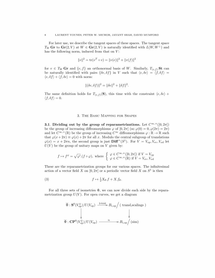
2.3. Geodesics leaving the space of immersions. Since geodesics on a sphereare always given by great circles, this theorem gives us the first case of explicitgeodesics on spaces of curves in the metric of this paper. However, note thatgreat circles in the open part S0 are susceptible to crossing the ‘bad’ part S−S0
somewhere. This occurs if and only if there exists θ such that (e + if)(θ) and(δe + iδf(θ)) have identical complex arguments modulo π. So we find that ourmetric on Imm is incomplete.
We can form a commutative diagram:
Φ : S0(V 2op)
2-fold //� _
��
Immop
/( transl,scalings )
� _
��
Φ : S(Vop) // C∞([0, 2π],C)/
(transl,scalings)
where we have denoted the extended Φ by Φ. For rather technical reasons Φ isnot surjective: there are pathological non-negative C∞ functions which have noC∞ square root, see [8], e.g. But what this diagram does do is give some space ofmaps to hold the extended geodesics. The example:
e(x, s) + if(x, s) = (x+ is)/√C, where
− π ≤ x ≤ π,−1 ≤ s ≤ 1 and C = 2a3/3 + 2as2
and c(x, s) = (x3/3− s2x+ isx2)/C − is/2 (suitably translated)
is shown in figure 1. This is a geodesic in which all curves are immersions fors 6= 0, but cx(x, 0) has a double zero at x = π.
2.4. The basic mapping in the periodic case. Next, consider the periodiccases. Here we need the Stiefel manifolds:
St(2, V ) = {orthonormal pairs (e, f) ∈ V × V }, V = Vev or Vod
and St0(2, V ) the subset defined by the constraint Z(e, f) = ∅. For later use, itis also convenient to note that St(2, V ) = {A ∈ L(C, V ) : AT .A = IdC} whereL(C, V ) is the space of linear maps from C to V and 〈A>v, w〉C = 〈v,Aw〉V . For(e, f) ∈ S0(V 2
op), when is c = Φ(e, f) periodic? If and only if we have:
c′ = 12 (e+ if)2 is periodic, so that e, f ∈ Vev or Vod;(A)
0 =
∫ 2π
0
c′(u) du =1
2
∫ 2π
0
(e2 − f2) du+ i
∫ 2π
0
ef du.(B)
Condition (B) says that ‖e‖2 = ‖f‖2 = 1 (since the sum is 2) and 〈e, f〉 =0, so that (e, f) ∈ St0(2, Vev) or (e, f) ∈ St0(2, Vod). Recall that the index nof an immersed curve c is defined by considering log(c′). The log must satisfylog(c′(θ + 2π)) ≡ log(c′(θ)) + 2πn for some n and this is the index. So this index

A METRIC ON SHAPE SPACE WITH EXPLICIT GEODESICS 7
Figure 1. The generic way in which a family of open immersions crosses
the hypersurface where Z 6= ∅. The parametrized straight line in the middle
of the family has velocity with a double zero at the black dot, hence is notan immersion. See text.
is even or odd depending on whether the square root of c′ is periodic or anti-periodic, that whether (e, f) ∈ Vev or ∈ Vod. So if Φ is restricted to St0(2, Vev) orSt0(2, Vod) (and is still denoted Φ), it provides isometric 2-fold coverings
Φ : St0(2, Vev) −→ {c ∈ Immev(S1,C) : c(0) = 0, `(c) = 1}Φ : St0(2, Vod) −→ {c ∈ Immod(S1,C) : c(0) = 0, `(c) = 1}
All three of these maps Φ can be modified so as to divide out by rotations. Themapping (e, f) 7→ eiϕ(e + if) produces a rotation of the immersed curve Φ(e, f)through an angle 2ϕ. The complex projective space CP(V 2
op) is S(V 2op) divided by
the action of rotations, and we denote by CP0(V 2op) the subset gotten by dividing
S0(V 2op) by rotations. The group generated by translations, rotations and scalings
will be called the group of similitudes, abreviated as ‘sim’. Then we get the variant:
Φ : CP0(V 2op) −→ Immop /(sim).
Similarly, let Gr(2, V ) be the Grassmannian of unoriented 2-dimensional sub-spaces of V and let Gr0(2, V ) be the subset of those W with Z(W ) = ∅ for V = Vev
or = Vod. Then we have maps:
Φ : Gr0(2, Vev) −→ Immev /(sim)
Φ : Gr0(2, Vod) −→ Immod /(sim)
8 LAURENT YOUNES, PETER W. MICHOR, JAYANT SHAH, DAVID MUMFORD
For later use, we describe the tangent spaces of these spaces. The tangent spaceTW Gr to Gr(2, V ) at W ∈ Gr(2, V ) is naturally identified with L(W,W⊥) andhas the following norm, induced from that on V :
‖v‖2 = tr(vT ◦ v) = ‖v(e)‖2 + ‖v(f)‖2
for v ∈ TW Gr and {e, f} an orthonormal basis of W . Similarly, T(e,f) St canbe naturally identified with pairs {δe, δf} in V such that 〈e, δe〉 = 〈f, δf〉 =〈e, δf〉+ 〈f, δe〉 = 0 with norm:
‖(δe, δf)‖2 = ‖δe‖2 + ‖δf‖2.
The same definition holds for T(e,f)(S), this time with the constraint 〈e, δe〉 +〈f, δf〉 = 0.
3. The Basic Mapping for Shapes
3.1. Dividing out by the group of reparametrizations. Let C∞,+([0, 2π])be the group of increasing diffeomorphisms ϕ of [0, 2π] (so ϕ(0) = 0, ϕ(2π) = 2π)and let C∞,+(R) be the group of increasing C∞ diffeomorphisms ϕ : R→ R suchthat ϕ(x+ 2π) ≡ ϕ(x) + 2π for all x. Modulo the central subgroup of translationsϕ(x) = x + 2πn, the second group is just Diff+(S1). For V = Vop, Vev, Vod letU(V ) be the group of unitary maps on V given by:
f 7→ fϕ =√ϕ′.(f ◦ ϕ), where
{ϕ ∈ C∞,+([0, 2π]) if V = Vop
ϕ ∈ C∞,+(R) if V = Vev, Vod
These are the reparametrization groups for our various spaces. The infinitesimalaction of a vector field X on [0, 2π] or a periodic vector field X on S1 is then
(3) f 7→ 12Xθ.f +X.fθ.
For all three sets of isometries Φ, we can now divide each side by the repara-metrization group U(V ). For open curves, we get a diagram
Φ : S0(V 2op)/U(Vop)
2-fold //
��
Bi,op
/( transl,scalings )
��
Φ : CP0(V 2op)/U(Vop)
≈ // Bi,op
/(sim)

A METRIC ON SHAPE SPACE WITH EXPLICIT GEODESICS 9
and a similar one for closed curves of even and odd index where V = Vev, Vod andB = Bi,ev, Bi,od:
Φ : St0(2, V )/U(V )2-fold //
��
B/
(transl,scalings)
��
Φ : Gr0(2, V )/U(V )≈ // B
/(sim)
Here we have divided by isometries on both the left and right: by U(V ) orU(V )×S1 on the left (where S1 rotates the basis {e, f}) and by reparametrizationsand rotations on the right. Thus Φ is again an isometry if we make both quotientsinto Riemannian submersions. This means we must identify the tangent spacesto the quotients with the horizontal subspaces of the tangent spaces in the largerspace, i.e. those perpendicular to the orbits of the isometric group actions. ForSt, this means:
3.2. Proposition. The tangent vector {δe, δf} to St satisfies:
〈δe, e〉 = 〈δf, f〉 = 0, 〈δe, f〉+ 〈δf, e〉 = 0.
It is horizontal for the rotation action if and only if:
both δe, δf are perpendicular to both e, f.
It is horizontal for the reparametrization group if:
Wθ(e, δe) +Wθ(f, δf) = 0
where Wθ(a, b) = a.bθ − b.aθ is the Wronskian with respect to the parameter θ.
Proof. Consider the action of rotations, which is one-dimensional, with orbitsβ 7→ eiβ(e + if); the direction at (e, f) is chosen as (−f, e). So (δe, δf) beinghorizontal at (e, f) for this action means that −〈f, δe〉+ 〈e, δf〉 = 0. This provesthe first assertion.
For the action of U(V ), one has to note that horizontal vectors must satisfy
〈 12Xθ.e+X.eθ, δe〉+ 〈 12Xθ.f +X.fθ, δf〉 = 0
for any periodic vector field X on R, which yields the horizontality condition afterintegration by parts of the terms in Xθ. �
Horizontality on the shape space side means (see [11]):
3.3. Proposition. h ∈ Tc Imm(S1,C) is horizontal for the action of Diff(S1) ifand only if D2
s(h) is normal to the curve, i.e. 〈v,D2s(h)〉 = 0.
3.4. Proposition. For any smooth path c in Imm(S1,R2) there exists a smoothpath ϕ in Diff(S1) with ϕ(0, . ) = IdS1 depending smoothly on c such that the pathe given by e(t, θ) = c(t, ϕ(t, θ)) is horizontal: 〈D2
s(et), eθ〉 = 0.

10 LAURENT YOUNES, PETER W. MICHOR, JAYANT SHAH, DAVID MUMFORD
This is a variant of [11, 4.6].
Proof. Writing Dc instead of Ds we note that Dc◦ϕ(f ◦ϕ) = (fθ◦ϕ)ϕθ|cθ◦ϕ|.|ϕθ| = (Dc(f))◦
ϕ for ϕ ∈ Diff+(S1). So we have Ln,c◦ϕ(f ◦ ϕ) = (Ln,cf) ◦ ϕ.
Let us write e = c◦ϕ for e(t, θ) = c(t, ϕ(t, θ)), etc. We look for ϕ as the integralcurve of a time dependent vector field ξ(t, θ) on S1, given by ϕt = ξ ◦ϕ. We wantthe following expression to vanish:
〈D2c◦ϕ(∂t(c ◦ ϕ)), ∂θ(c ◦ ϕ)〉 = 〈D2
c◦ϕ(ct ◦ ϕ+ (cθ ◦ ϕ)ϕt), (cθ ◦ ϕ)ϕθ〉= 〈D2
c (ct) ◦ ϕ+D2c (cθ.ξ) ◦ ϕ, cθ ◦ ϕ〉ϕθ
=((〈D2
c (ct), cθ〉+ 〈D2c (ξ.cθ), cθ〉) ◦ ϕ
)ϕθ.
Using the time dependent vector field ξ = − 1|cθ|D
−2c (〈D2
c (ct), v〉) and its flow ϕ
achieves this. �
3.5. Bigger spaces. As we will see below, we can describe geodesics in the ‘clas-sical’ spaces S,CP,St,Gr quite explicitly. By the above isometries, this givesus the geodesics in the various spaces Imm, Bi. BUT, as we mentioned above forthe space S, geodesics in the ‘good’ parts S0,CP0,St0,Gr0 do not stay there,but they cross the ‘bad’ part where Z(e, f) 6= ∅. Now the basic mapping is stilldefined on the full sphere, projective space, Stiefel manifold or Grassmannian, giv-ing us some smooth mappings of [0, 2π] or S1 to C, possibly modulo translations,rotations and/or scalings.
But when we divide by U(Vop), a major problem arises. The orbits of U(Vop)acting on C∞([0, 2π],C) are not closed, hence the topological quotient of the spaceC∞([0, 2π],C) by U(Vop) is not Hausdorff. This is shown by the following con-struction:
(1) Start with a C∞ non-decreasing map ψ from [0, 2π] to itself such thatψ(θ) ≡ π for θ in some interval I.
(2) Let ψn(θ) = (1− 1/n).ψ(θ) + θ/n. The sequence {ψn} of diffeomorphismsof [0, 2π] converges to ψ.
(3) Then for any c ∈ Immop, the maps c ◦ ψn are all in the orbit of c. Butthey converge to c ◦ ψ which is constant on the whole interval I, hence isnot in the orbit.
Thus, if we want some Hausdorff space of curves which a) have singularities morecomplex than those of immersed curves and b) can hold the extensions of geodesicsin some space Bi which come from the map Φ, we must divide C∞([0, 2π],C) bysome equivalence relation larger than the group action by U(V ). The simplestseems to be: first define a monotone relation R ⊂ [0, 2π]× [0, 2π] to be any closedsubset such that p1(R) = p2(R) = [0, 2π] (p1 and p2 being the projections on theaxes) and for every pair of points (s1, t1) ∈ R and (s2, t2) ∈ R, either s1 ≤ s2 and

A METRIC ON SHAPE SPACE WITH EXPLICIT GEODESICS 11
t1 ≤ t2 or vice versa. Then f, g : [0, 2π] → C are Frechet equivalent if there is amonotone relation R such that f(s) = g(t),∀(s, t) ∈ R.
This is a good equivalence relation because if {fn}, {gn} : [0, 2π] → C are twosequences and limn fn = f, limn gn = g and fn, gn are Frechet equivalent for alln, then f, g are Frechet equivalent. The essential point is that the set of non-empty closed subsets of a compact metric space X is compact in the Hausdorfftopology (see [1]). Thus if {Rn} are the monotone relations instantiating theequivalence of fn and gn, a subsequence {Rnk} Hausdorff converges to some R ⊂[0, 2π]× [0, 2π] and it is immediate that R is a monotone relation making f and gFrechet equivalent.
Define
Bbig,op = C∞([0, 2π],C)/Frechet equivalence, translations, scalings.
Then we have a commutative diagram:
Φ : S0(V 2op) //� _
��
Bi,op
/(transl,scalings )
� _
��Φ : S(V 2
op) // Bbig,op
Thus the whole of a geodesic which enters the ‘bad’ part of S(Vop) creates a pathin Bbig,op. Of course, the same construction works for closed curves also. We willsee several examples in the next section.
4. Construction of Geodesics
4.1. Great circles in Spheres. The space S(V 2) being the sphere of radius√
2on V 2, its geodesics are the great circles. Thus, the geodesic distance between(e0, f0) and (e1, f1) is given by
√2D with
D = arccos((⟨e0 , e1
⟩+⟨f0 , f1
⟩)/2)
and the geodesic is given by
e(t) =sin((1− t)D)
sinDe0 +
sin(tD)
sinDe1
f(t) =sin((1− t)D)
sinDf0 +
sin(tD)
sinDf1
The corresponding geodesic on Immop modulo translation and scaling is the time-indexed family of curves t 7→ c(u, t) with
∂c/∂u = 12 (e(t) + if(t))2 = (e(t)2 − f(t)2)/2 + ie(t)f(t)

12 LAURENT YOUNES, PETER W. MICHOR, JAYANT SHAH, DAVID MUMFORD
The following notation will be used throughout this section:
c0(u) = c(u, 0), c1(u) = c(u, 1)
∂c0/∂u = r0(u)eiα0(u), ∂c1/∂u = r1(u)eiα
1(u)
so that ej =√
2rj cos αj
2 and f j =√
2rj sin αj
2 for j = 0, 1. Thus the distance Dis
Dop(c0, c1) = arccos
∫ 2π
0
√r0r1 cos
α1 − α0
2du.
The metric on Immop modulo rotations is
Dop, rot(c0, c1) = inf
αarccos
∫ 2π
0
√r0r1 cos
α1 − α0 − α2
du
= arccos supα
∫ 2π
0
√r0r1
(cos
α1 − α0
2cos
α
2+ sin
α1 − α0
2sin
α
2
)du
= arccos
((∫ 2π
0
√r0r1 cos
α1 − α0
2du)2
+(∫ 2π
0
√r0r1 sin
α1 − α0
2du)2)1/2
The distance on Bi,op is the infimum of this expression over all changes ofcoordinate for c0. Assuming that c0 and c1 are originally parametrized with 1/2πtimes arc-length so that r0 ≡ 1/2π, r1 ≡ 1/2π, this is
(4) Dop, diff(c0, c1) = arccos supφ
1
2π
∫ 2π
0
√φθ cos
α1 ◦ φ− α0
2dθ
and modulo rotations
Dop, diff, rot(c0, c1) = arccos sup
φ
(( 1
2π
∫ 2π
0
√φθ cos
α1 ◦ φ− α0
2dθ)2
+( 1
2π
∫ 2π
0
√φθ sin
α1 ◦ φ− α0
2dθ)2)1/2
.
The supremum in both expressions is taken over all increasing bijections φ ∈C∞([0, 2π], [0, 2π]).
To shorten these formulae, we will use the following notation. Define:
C−(φ) =1
2π
∫ 2π
0
√φθ cos
α1 ◦ φ− α0
2dθ
S−(φ) =1
2π
∫ 2π
0
√φθ sin
α1 ◦ φ− α0
2dθ
Then we have:
Dop, diff = infφ
arccos(C−(φ)) and
Dop, diff, rot = infφ
arccos(√
(C−(φ))2 + (S−(φ))2).

A METRIC ON SHAPE SPACE WITH EXPLICIT GEODESICS 13
4.2. Problems with the existence of geodesics. These expressions give veryexplicit descriptions of distance and geodesics. We have already noted, however,that, even if both (e0, f0) and (e1, f1) belong to S0, the same property is notguaranteed at each point of the geodesic. e(α, t) = f(α, t) = 0 happens for some twhenever (e0(α), f0(α)) and (e1(α), f1(α)) are collinear with opposite orientations.This is not likely to happen for geodesics joining nearby points. When it doeshappen, it is usually a stable phenomenon: for example, if the geodesic crossesS−S0 transversally, as illustrated in figure 1, then this happens for all nearbygeodesics too. Note that this means that the geodesic spray on Immop is not
surjective. In fact, any geodesic on Immop comes from a great circle on S0 and if
it crosses S−S0, it leaves Immop.
When we pass to the quotient by reparametrizations, another question arises:does the inf over reparametrizations exist? or equivalently is there is a horizontalgeodesic joining any two open curves? In fact, there need not be any such geodesiceven if you allow it to cross S−S0. In general, to obtain a geodesic minimizingdistance between 2 open curves, the curves themselves must be given parametriza-tions with zero velocity somewhere, i.e. they may need to be lifted to points inS−S0.
This is best illustrated by the special case in which c1 is the line segment from0 to 1, namely e1 + if1 = 1/
√π, α1 ≡ 0. The curve c0 can be arbitrary. Then the
reparametrization φ which minimizes distance is the one which maximizes:∫ 2π
0
√φθ cos
α0
2dθ.
This variational problem is easy to solve: the optimal φ is given by:
φ(u) = 2π
∫ u
0
max
(cos
α0
2, 0
)2/∫ 2π
0
max
(cos
α0
2, 0
)2
.
Note that φ is not in general a diffeomorphism: it is constant on intervals wherecos(α0/2) ≤ 0. Its graph is a monotone relation in the sense of section 3.5. In fact,it’s easy to see that monotone relations enjoy a certain compactness, so that theinf over reparametrizations is always achieved by a monotone relation. Assumingα0 is represented by a continuous function for which −2π < α0(u) < 2π, the resultis that the places on the curve c0 where |α0(u)| > π get squashed to points on theline segment. The result is that this limit geodesic is not actually a path in thespace B of smooth curves. Figure 2 illustrates this effect.
The general problem of maximizing the functional
U(φ) =1
2π
∫ 2π
0
√φθ cos
α1 ◦ φ− α0
2dθ

14 LAURENT YOUNES, PETER W. MICHOR, JAYANT SHAH, DAVID MUMFORD
with respect to increasing functions φ has been addressed in [17]. Existence ofsolutions can be shown in the class of monotone relations, or, equivalently func-tions φ that take the form φ(s) = µ([0, s)) for some positive measure µ on [0, 2π]with total mass less or equal to 2π (φθ being replaced by the Radon-Nykodimderivative of µ in the definition of U). The optimal φ is a diffeomorphism as soonas cos((α1(u)− α0(v))/2) > 0 whenever |u− v| is smaller than a constant (whichdepends on α0 and α1). More details can be found in [17].
It is easy to show that maximizing U is equivalent to maximizing
U+(φ) =1
2π
∫ 2π
0
√φθ max
(cos
α1 ◦ φ− α0
2, 0
)dθ
because one can always modify φ on intervals on which cos((α1 ◦ φ − α0)/2) < 0to ensure that φθdθ = 0. In [18], it is proposed to maximize
U(φ) =1
2π
∫ 2π
0
√φθ
∣∣∣∣cosα1 ◦ φ− α0
2
∣∣∣∣ dθ.This corresponds to replacing the lift e(u) + if(u) by σ(u).(e(u) + if(u)) whereσ(u) = ± for all u, but this is beyond the scope of this paper.
100−fold blow−up in middle
Figure 2. This is a geodesic of open curves running from the curve withthe kink at the top left to the straight line on the bottom right. A blow upof the next to last curve is shown to reveal that the kink never goes away – it
merely shrinks. Thus this geodesic is not continuous in the C1-topology onBop. The straight line is parametrized so that it stops for a whole interval of
time when it hits the middle point and thus it is C1-continuous in Immop.

A METRIC ON SHAPE SPACE WITH EXPLICIT GEODESICS 15
4.3. Neretin geodesics on Gr(2, V ). The integrated path-length distance andexplicit geodesics can be found in any Grassmannian using Jordan Angles [13]as follows: If W0,W1 ⊂ V are two 2-dimensional subspaces the singular valuedecomposition of the orthogonal projection p of W0 to W1 gives orthonormal bases{e0, f0} of W0 and {e1, f1} of W1 such that p(e0) = λe.e
1, p(f0) = λff1, e0 ⊥ f1
and f0 ⊥ e1, where 0 ≤ λf , λe ≤ 1. Write λe = cos(ψe), λf = cos(ψf ) then ψe, ψfare the Jordan angles, 0 ≤ ψe, ψf ≤ π/2. The global metric is given by:
d(W 0,W 1) =√ψ2e + ψ2
f
and the geodesic by:
(5) W (t) =
e(t) =
sin((1− t).ψe)e0 + sin(tψe)e1
sinψe,
f(t) =sin((1− t).ψf )f0 + sin(tψf )f1
sinψf
.
We apply this now in order to compute the distance between the curves inthe two spaces Immev /(sim) and Immod /(sim), as well as in the unparametrized
quotients Bi,ev/(sim) and Bi,od/(sim). We write as above ∂θc0 = r0(θ)eiα
0(θ) and
∂θc1 = r1(θ)eiα
1(θ). We put
e0 =√
2r0 cos α0
2 f0 =√
2r0 sin α0
2 ,
e1 =√
2r1 cos α1
2 f1 =√
2r1 sin α1
2
thus lifting these curves to 2-planes in the Grassmannian. The 2× 2 matrix of theorthogonal projection from the space {e0, f0} to {e1, f1} in these bases is:
M(c0, c1) =
∫S1 2√r0.r1. cos α
0
2 cos α1
2 dθ∫S1 2√r0.r1. cos α
0
2 sin α1
2 dθ∫S1 2√r0.r1. sin α0
2 cos α1
2 dθ∫S1 2√r0.r1. sin α0
2 sin α1
2 dθ
It will be convenient to use the notations:
C± :=
∫S1
√r0.r1 cos α
0±α1
2 dθ = 12
(M(c0, c1)11)∓M(c0, c1)22
)S± :=
∫S1
√r0.r1 sin α0±α1
2 dθ = 12
(M(c0, c1)21 ±M(c0, c1)12
)We have to diagonalize this matrix by rotating the curve c0 by a constant angle
β0, i.e., the basis {e0, f0} by the angle β0/2; and similarly the curve c1 by aconstant angle β1. So we have to replace α0 by α0−β0 and α1 by α1−β1 in sucha way that
0 =
∫S1
√r0.r1 sin
((α0 − β0)± (α1 − β1)
2
)dθ (for both signs)(6)
= S±. cos β0±β1
2 − C±. sin β0±β1
2

16 LAURENT YOUNES, PETER W. MICHOR, JAYANT SHAH, DAVID MUMFORD
Thusβ0 ± β1 = 2 arctan (S±/C±) .
In the newly aligned bases, the diagonal elements of M(c0, c1) will be the cosinesof the Jordan angles. But even without preliminary diagonalization, the followinglemma gives you a formula for them:
Lemma. If M =
(a bc d
)and C± = 1
2 (a∓ d), S± = 12 (c± b), then the singular
values of M are: √C2− + S2
− ±√C2
+ + S2+.
The proof is straightforward. This gives the formula
Dod,rot(c0, c1)2 = arccos2
(√S2
+ + C2+ +
√S2− + C2
−
)(7)
+ arccos2(√
S2− + C2
− −√S2
+ + C2+
).
This is the distance in the space Immod(S1,C)/(transl, rot., scalings).
4.4. Horizontal Neretin distances. If we want the distance in the quotientspace Bi,od/(transl, rot., scalings) by the group Diff(S1) we have to take the infi-mum of (7) over all reparametrizations. To simplify the formulas that follow, wecan assume that the initial curves c0, c1 are parametrized by arc length so thatr0 ≡ r1 ≡ 1/2π. Then consider a reparametrization φ ∈ Diff(S1) of one of the twocurves, say c0 ◦ φ:
(8) Dsim,diff(c0, c1)2 = infφ
(arccos2(λe(c
0 ◦ φ, c1)) + arccos2(λf (c0 ◦ φ, c1)))
where now
λe(c0 ◦ φ, c1) =
√S2−(φ) + C2
−(φ) +√S2
+(φ) + C2+(φ)
λf (c0 ◦ φ, c1) =√S2−(φ) + C2
−(φ)−√S2
+(φ) + C2+(φ)
S±(φ) :=1
2π
∫S1
√φθ sin (α0◦φ)±α1
2 dθ,
C±(φ) :=1
2π
∫S1
√φθ cos (α0◦φ)±α1
2 dθ.
To describe the inf, we can use the fact that geodesics on the space of curvesare the horizontal geodesics in the space of immersions. Consider the geodesict 7→ {e(t), f(t)} in Gr(2, V ) described in (5), for
e0 =√
φθπ cos (α0◦φ)−β0
2 e1 = 1√π
cos α1−β1
2 ,
f0 =√
φθπ sin (α0◦φ)−β0
2 f1 = 1√π
sin α1−β1
2 ,

A METRIC ON SHAPE SPACE WITH EXPLICIT GEODESICS 17
where the rotations β0 and β1 must be computed from c0 ◦ φ and c1. Note that
e0θ =
φθθ
2√πφθ
cos (α0◦φ)−β0
2 − 12√πφ
3/2θ .(α0
θ ◦ φ). sin (α0◦φ)−β0
2 ;
e1θ = −1
2√π.α1θ. sin
α1−β1
2
f0θ =
φθθ
2√πφθ
sin (α0◦φ)−β0
2 + 12√πφ
3/2θ .(α0
θ ◦ φ). cos (α0◦φ)−β0
2 ;
f1θ = 1
2√π.α1θ. cos α
1−β1
2
If the Jordan angles are ψe and ψf , then the tangent vector to the geodesic t 7→W (t) at t = 0 is described by
et(0) = ∂t|0e =ψe
sinψe.(e1 − cosψe.e
0), ft(0) = ∂t|0f =
ψfsinψf
.(f1 − cosψf .f
0)
By 3.2 the geodesic is perpendicular to all Diff(S1)-orbits if and only if the sumof Wronskians vanishes:
0 = Wθ(e0, et(0)) +Wθ(f
0, ft(0)) =
= e0 ψesinψe
(e1θ − cosψee
0θ
)− e0
θ
ψesinψe
(e1 − cosψee
0)
+ f0 ψfsinψf
(f1θ − cosψff
0θ
)− f0
θ
ψfsinψf
(f1 − cosψff
0)
=ψe
sinψeWθ(e
0, e1) +ψf
sinψfWθ(f
0, f1)
= − 1√φθ
{φθθ
( ψesinψe
cos (α0◦φ)−β0
2 cos α1−β1
2 +ψf
sinψfsin (α0◦φ)−β0
2 sin α1−β1
2
)− φθα1
θ
( ψesinψe
cos (α0◦φ)−β0
2 sin α1−β1
2 − ψfsinψf
sin (α0◦φ)−β0
2 cos α1−β1
2
)+ φ2
θ(α0θ ◦ φ)
( ψesinψe
sin (α0◦φ)−β0
2 cos α1−β1
2 − ψfsinψf
cos (α0◦φ)−β0
2 sin α1−β1
2
)}This is an ordinary differential equation for φ which is coupled to the (integral)equations for calculating the β’s as functions of φ. If it is non-singular (i.e., thecoefficient function of φθθ does not vanish for any θ) then there is a solution φ,at least locally. But the non-existence of the inf described for open curves abovewill also affect closed curves and global solutions may actually not exist. However,for closed curves that do not double back on themselves too much, as we will see,geodesics do seem to usually exist.
4.5. An Example. Geodesics in the sphere are great circles, which go all theway around the sphere and are always closed geodesics. In the case of the Grass-mannian, using the Jordan angle basis, the geodesic can be continued indefinitelyusing formula 5 above. In fact, it will be a closed geodesic if the Jordan angles
18 LAURENT YOUNES, PETER W. MICHOR, JAYANT SHAH, DAVID MUMFORD
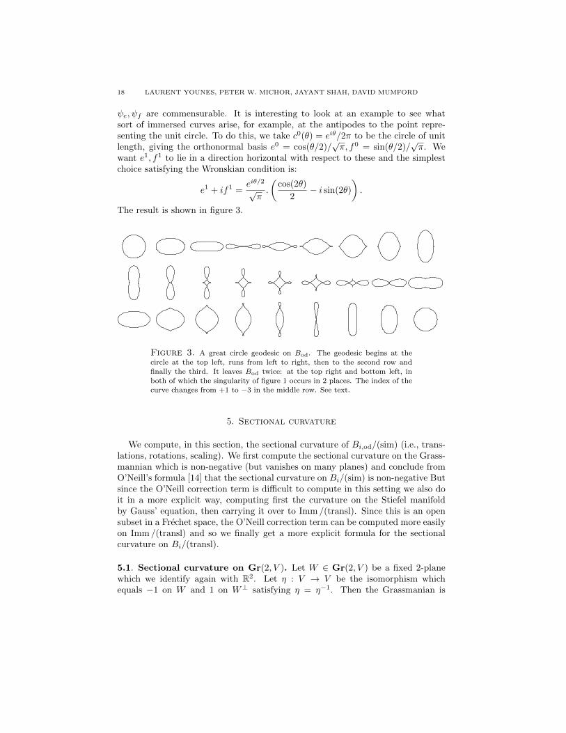
ψe, ψf are commensurable. It is interesting to look at an example to see whatsort of immersed curves arise, for example, at the antipodes to the point repre-senting the unit circle. To do this, we take c0(θ) = eiθ/2π to be the circle of unitlength, giving the orthonormal basis e0 = cos(θ/2)/
√π, f0 = sin(θ/2)/
√π. We
want e1, f1 to lie in a direction horizontal with respect to these and the simplestchoice satisfying the Wronskian condition is:
e1 + if1 =eiθ/2√π.
(cos(2θ)
2− i sin(2θ)
).
The result is shown in figure 3.
Figure 3. A great circle geodesic on Bod. The geodesic begins at thecircle at the top left, runs from left to right, then to the second row and
finally the third. It leaves Bod twice: at the top right and bottom left, in
both of which the singularity of figure 1 occurs in 2 places. The index of thecurve changes from +1 to −3 in the middle row. See text.
5. Sectional curvature
We compute, in this section, the sectional curvature of Bi,od/(sim) (i.e., trans-lations, rotations, scaling). We first compute the sectional curvature on the Grass-mannian which is non-negative (but vanishes on many planes) and conclude fromO’Neill’s formula [14] that the sectional curvature on Bi/(sim) is non-negative Butsince the O’Neill correction term is difficult to compute in this setting we also doit in a more explicit way, computing first the curvature on the Stiefel manifoldby Gauss’ equation, then carrying it over to Imm /(transl). Since this is an opensubset in a Frechet space, the O’Neill correction term can be computed more easilyon Imm /(transl) and so we finally get a more explicit formula for the sectionalcurvature on Bi/(transl).
5.1. Sectional curvature on Gr(2, V ). Let W ∈ Gr(2, V ) be a fixed 2-planewhich we identify again with R2. Let η : V → V be the isomorphism whichequals −1 on W and 1 on W⊥ satisfying η = η−1. Then the Grassmanian is
A METRIC ON SHAPE SPACE WITH EXPLICIT GEODESICS 19
the symmetric space O(V )/(O(W ) × O(W⊥)) with the involutive automorphismσ : O(V )→ O(V ) given by σ(U) = η.Uη. For the Lie algebra in the V = W⊕W⊥-decomposition we have(
−1 00 1
)(x −yTy U
)(−1 00 1
)=
(x yT
y U
)Here x ∈ L(W,W ), y ∈ L(W,W⊥). The fixed point group is O(V )σ = O(W ) ×O(W⊥). The reductive decomposition g = k + p is given by{(
x −yTy U
)}=
{(x 00 U
), x ∈ so(2)
}+
{(0 −yTy 0
), y ∈ L(W,W⊥)
}Let π : O(V ) → O(V )/(O(W )× O(W⊥)) = Gr(2, V ) be the quotient projection.Then Teπ : p → To Gr is an isomorphism, and the O(V )-invariant Riemannianmetric on Gr(2, V ) is given by
GGro (Teπ.Y1, Teπ.Y2) = − 1
2 tr(Y1Y2) = − 12 tr
(0 −yT1y1 0
)(0 −yT2y2 0
)= − 1
2 tr
(−yT1 y2 0
0 −y1yT2
)= 1
2 trW (yT1 y2) + 12 trW⊥(y1y
T2 )
= trW (yT1 y2) = 〈y1(e1), y2(e1)〉W⊥ + 〈y1(e2), y2(e2)〉W⊥
for Y1, Y2 ∈ p, where e1, e2 is an orthonormal base of W . By the general theory ofsymmetric spaces [6], the curvature is given by
RGro (Teπ.Y1, Teπ.Y2)Teπ.Y1 = Teπ.[[Y1, Y2], Y1][(
0 −yT1y1 0
),
(0 −yT2y2 0
)]=
(−yT1 y2 + yT2 y1
0 −y1yT2 + y2y
T1
)[[(
0 −yT1y1 0
),
(0 −yT2y2 0
)],
(0 −yT1y1 0
)]=
=
[(−yT1 y2 + yT2 y1 0
0 −y1yT2 + y2y
T1
),
(0 −yT1y1 0
)]=
(0 2yT1 y2y
T1 − yT2 y1y
T1 − yT1 y1y
T2
−2y1yT2 y1 + y2y
T1 y1 + y1y
T1 y2 0
)For the sectional curvature we have (where we assume that Y1, Y2 is orthonormal):
kGr(2,V )span(Y1,Y2) = −B(Y2, [[Y1, Y2], Y1]) = trW (yT2 y2y
T1 y1 + yT2 y1y
T1 y2 − 2yT2 y1y
T2 y1)
= 12 trW
((yT2 y1 − yT1 y2)T (yT2 y1 − yT1 y2)
)+ 1
2 trW⊥((y2y
T1 − y1y
T2 )T (y2y
T1 − y1y
T2 ))
= 12‖y
T2 y1 − yT1 y2‖2L2(W,W ) + 1
2‖y2yT1 − y1y
T2 ‖2L2(W⊥,W⊥) ≥ 0.
where L2 stands for the space of Hilbert-Schmidt operators. Note that there aremany orthonormal pairs Y1, Y2 on which sectional curvature vanishes and that its

20 LAURENT YOUNES, PETER W. MICHOR, JAYANT SHAH, DAVID MUMFORD
maximum value 2 is attained when yi are isometries and y2 = Jy1 where J isrotation through angle π/2 in the image plane of y1.
5.2. Sectional curvature on Imm/(sim). The curvature formula can be rewrit-ten by ‘lowering the indices’ which will make it much easier to express it in termsof the immersion c. Fix an orthonormal basis e, f of W and let δek = yk(e), δfk =yk(f). For x, y ∈ W⊥, we use the notation x ∧ y = x ⊗ y − y ⊗ x ∈ W⊥ ⊗W⊥.Then:
kGr(2,V )span(Y1,Y2) = (〈δe1, δf2〉 − 〈δe2, δf1〉)2 + 1
2‖δe1 ∧ δe2 + δf1 ∧ δf2‖2.
To check this, note that yT2 y1 − yT1 y2 is given by a skew-symmetric 2 × 2 matrixwhose off diagonal entry is just 〈δe1, δf2〉 − 〈δe2, δf1〉 and this identifies the firstterms in the two formulas for k. On the other hand, y2y
T1 is given by a matrix of
rank 2 on the infinite dimensional space W⊥. In view of W⊥⊗W⊥ ⊂ L(W⊥,W⊥)it is the 2-tensor δe1⊗ δe2 + δf1⊗ δf2. Skew-symmetrizing, we identify the secondterms in the two expressions for k.
Going over to the immersion c, the tangent vector δek + iδfk to Gr becomesthe tangent vector hk = δc =
∫(δek + iδfk)(e + if)dθ to Imm/(sim). To express
the first term in the curvature, we have:
Proposition. 〈δe1, δf2〉 − 〈δe2, δf1〉 =∫C
det(Dsh1, Dsh2)ds.
Proof.
Ds(hk) =(e+ if).(δek + iδfk)
e2 + f2
hence
det(Dsh1, Dsh2) = Im(Dsh1, Dsh2) =Im ((δe1 − iδf1)(δe2 + iδf2))
e2 + f2
hence ∫C
det(Dsh1, Dsh2)ds =
∫S1
(δe1δf2 − δe2δf1)dθ.
�
The second term is not quite so compact: because it is a norm on W⊥ ⊗W⊥,it requires double integrals over C ×C, not just a simple integral over C. We usethe notation as above c(θ) = r(θ)eiα(θ). Then we have:
Proposition.
‖δe1 ∧ δe2 + δf1 ∧ δf2‖2 = term1 + term2
term1 =
∫∫C×C
1 + cos(α(x)− α(y))
2·(〈Dsh1(x), Dsh2(y)〉−〈Dsh2(x), Dsh1(y)〉
)2
ds(x)ds(y)

A METRIC ON SHAPE SPACE WITH EXPLICIT GEODESICS 21
term2 =
∫∫C×C
1− cos(α(x)− α(y))
2·(
det(Dsh1(x), Dsh2(y))−det(Dsh2(x), Dsh1(y))
)2
ds(x)ds(y)
Proof. Using r and α, we have:√re−iα/2Dshk = δek + iδfk, hence:√
r(x)r(y)ei(α(x)−α(y)
2 Dsh1(x)Dsh2(y) = δe1(x)δe2(y) + δf1(x)δf2(y) + i(· · · )
Skew-symmetrizing in the 2 vectors h1, h2, we get:√r(x)r(y)Re
{ei(α(x)−α(y))
2
(Dsh1(x)Dsh2(y)−Dsh2(x)Dsh1(y)
)}=
δe1(x)δe2(y)− δe2(x)δe1(y) + δf1(x)δf2(y)− δf2(x)δf1(y).
Squaring and integrating over S1 × S1, the right hand becomes ‖δe1 ∧ δe2 + δf1 ∧δf2‖2. On the left, first write Re(ei(α(x)−α(y))/2(· · · )) as the sum of cos((α(x) −α(y))/2)Re(· · · ) and − sin((α(x) − α(y))/2)Im(· · · ). Then when we square andintegrate, the cross term drops out because it is odd when x, y are reversed. �
We therefore obtain the expression of the curvature in Imm/(sim):
kImm /(sim)span(h1,h2) =
(∫C
det(Dsh1, Dsh2)ds)2
+
+
∫∫C×C
1 + cos(α(x)− α(y))
2·(〈Dsh1(x), Dsh2(y)〉−〈Dsh2(x), Dsh1(y)〉
)2
ds(x)ds(y)+(9)
+
∫∫C×C
1− cos(α(x)− α(y))
2·(
det(Dsh1(x), Dsh2(y))−det(Dsh2(x), Dsh1(y))
)2
ds(x)ds(y)
A major consequence of the calculation for the curvature on the Grassmannianis:
5.3. Theorem. The sectional curvature on Bi/(sim) is ≥ 0.
Proof. We apply O’Neill’s formula [14] to the Riemannian submersion
π : Gr0 → Gr0 /U(V ) ∼= Bi/Diff+(S1)
kGr0/U(V )π(W ) (X,Y ) = kGr0
W (Xhor, Y hor) + 34‖[X
hor, Y hor]ver|W ‖2 ≥ 0
where Xhor is a horizontal vector field projecting to a vector field X at π(W );similarly for Y . The horizontal and vertical projections exist and are pseudodifferential operators, see 5.6. �

22 LAURENT YOUNES, PETER W. MICHOR, JAYANT SHAH, DAVID MUMFORD
5.4. Sectional curvature on St(2, V ). The Stiefel manifold is not a symmetricspace (as the Grassmannian); it is a homogeneous Riemannian manifold. This canbe used to compute its sectional curvature. But the following procedure is simpler:
For (e, f) ∈ V 2 we consider the functions
Q1(e, f) =1
2‖e‖2, Q2(e, f) =
1
2‖f‖2 and Q3(e, f) =
1√2〈e , f〉.
Then St(2, V ) is the codimension 3 submanifold of V 2 defined by the equationsQ1 = Q2 = 1/2, Q3 = 0.
The metric on St(2, V ) is induced by the metric on V 2. If ξ1 = (δe1, δf1)and ξ2 = (δe2, δf2) are tangent vectors at a point in V 2, we have 〈ξ1 , ξ2〉 =〈δe1 , δe2〉 + 〈δf1 , δf2〉. For a function ϕ on V 2 its gradient gradϕ of ϕ (if itexists) is given by 〈gradϕ(v), ξ〉 = dϕ(v)(ξ) = Dv,ξϕ. The following are thegradients of Qi:
gradQ1 = (e, 0), gradQ2 = (0, f), gradQ3 =1√2
(f, e),
and these form an orthonormal basis of the normal bundle Nor(St) of St(2, V ).Let ξ1, ξ2 be two normal unit vectors tangent to St(2, V ) at a point (e, f). SinceV 2 is flat the sectional curvature of St(2, V ) is given by the Gauss formula [4]:
kSt(2,V )span(ξ1,ξ2) = 〈S(ξ1, ξ1), S(ξ2, ξ2)〉 − 〈S(ξ1, ξ2), S(ξ1, ξ2)〉
where S denotes the second fundamental form of St(2, V ) in V 2. Moreover, whena manifold is given as the zeros of functions Fk in a flat ambient space whosegradients are orthonormal, the second fundamental form is given by:
S(X,Y ) =∑k
HFk(X,Y ) · gradFk
where H is the Hessian of second derivatives. Given ξ1, ξ2 ∈ T(e,f) St with ξi =(δei, δfi), we have:
HQ1(ξ1, ξ2) = 〈δe1, δe2〉, HQ2(ξ1, ξ2) = 〈δf1, δf2〉,HQ3(ξ1, ξ2) = 1√
2
(〈δe1, δf2〉+ 〈δe2, δf1〉
)so that
S(ξ1, ξ2) = −〈δe1, δe2〉 gradQ1 − 〈δf1, δf2〉 gradQ2
− 1√2
(〈δf1, δe2〉+ 〈δe1, δf2〉
)gradQ3.
Finally, the sectional curvature of St(2, V ) for a normal pair of unit vectors ξ, ηin Tf St(2, V ) is given by:
kSt(2,V )span(ξ1,ξ2) = ‖δe1‖2‖δe2‖2 + ‖δf1‖2‖δf2‖2 + 2〈δe1, δf1〉〈δe2, δf2〉
− 〈δe1, δe2〉2 − 〈δf1, δf2〉2 − 12 (〈δe1, δf2〉+ 〈δf1, δe2〉)2

A METRIC ON SHAPE SPACE WITH EXPLICIT GEODESICS 23
= 12‖δe1 ⊗ δe2 − δe2 ⊗ δe1 + δf1 ⊗ δf2 − δf2 ⊗ δf1‖2(10)
− 12 (〈δe1, δf2〉 − 〈δe2, δf1〉)2
Comparing this with the curvature for the Grasmannian, we see that the O’Neillfactor in this case is 3
2 (〈δe1, δf2〉 + 〈δf1, δe2〉)2. Moreover, we can write for thecurvature of the isometric Imm/(transl, scal)
kImm/(transl,scal)span(h1,h2) = − 1
2
(∫C
det(Dsh1, Dsh2)ds
)2
+
+ 12
∫∫C×C
1 + cos(α(x)− α(y))
2·(〈Dsh1(x), Dsh2(y)〉−−〈Dsh2(x), Dsh1(y)〉
)2
ds(x)ds(y)+(11)
+ 12
∫∫C×C
1− cos(α(x)− α(y))
2·(
det(Dsh1(x), Dsh2(y))−−det(Dsh2(x), Dsh1(y))
)2
ds(x)ds(y)
5.5. Sectional curvature on the unscaled Stiefel manifold. Using the basicmapping Φ, the manifold Imm /(transl) can be identified with the unscaled Stiefelmanifold which we view as the following submanifold of V 2. We do not introducea systematic notation for it.
(12) M = {(e, f) ∈ V 2 \ {(0, 0)}, ‖e‖2 = ‖f‖2 and 〈e , f〉 = 0}
equipped with the metric
‖(δe, δf)‖2(e,f) = 2‖δe‖2 + ‖δf‖2
‖e‖2 + ‖f‖2.
Consider the diffeomorphism Ψ : R+ × St(2, V )→M defined by
Ψ(`, (e, f)) = (√`.e,√`.f) =: (e, f).
For ξ(δe, δf) ∈ T(e,f) St we have
T(`,e,f)Ψ.(λ, ξ) =( λ
2√`e+√`.δe,
λ
2√`f +√`.δf
)=: (δe, δf)
Thus, Ψ is an isometry if R+ × St(2, V ) is equipped with the metric
‖(λ, ξ)‖2`,(e,f) =λ2
2`2+ ‖δe‖2 + ‖δf‖2
so that M is isometric to the Riemannian product of R+ and St(2, V ), taking
‖λ‖` = |λ|/(√
2.`) for the metric on R+. This implies that the curvature tensoron M is the sum of the tensors on R+ (which vanishes) and St(2, V ). Thus, ifξi = T(`,f)π.(λ, ξi), i = 1, 2 with (ξ1, ξ1) orthonormal,
kMspan(ξ1,ξ2) =−〈RM (ξ1, ξ2)ξ1, ξ2〉‖ξ1‖2‖ξ2‖2 − 〈ξ1, ξ2〉2
=−〈RSt(ξ1, ξ2)ξ1, ξ2〉‖ξ1‖2‖ξ2‖2 − 〈ξ1, ξ2〉2
24 LAURENT YOUNES, PETER W. MICHOR, JAYANT SHAH, DAVID MUMFORD
=kStspan(ξ1,ξ2)
‖ξ1‖2‖ξ2‖2 − 〈ξ1, ξ2〉2
Note that we have the relations:
δe =λ
2√`e+√`.δe(13)
δf =λ
2√`f +√`.δf
(14)
5.6. O’Neill’s formula. For Riemannian submersions, O’Neill formula [14] statesthat the sectional curvature, in the plane generated by two horizontal vectors, isgiven by the curvature computed on the space “above” plus a positive correctionterm given by (3/4) times the squared norm of the vertical projection of the Liebracket of any horizontal extensions of the two vectors. We now proceed to thecomputation of this correction for the submersion from Imm /(sim) to Bi/(sim).
Because of the simplicity of local charts there, it will be easier to start fromImm /(transl). Let c ∈ Imm with
∫S1 c ds = 0. We first compute the vertical
projection of a vector h ∈ Tc Imm /(transl) for the submersion Imm /(transl) →Bi/(sim). Vectors in the vertical space at c take the form
h = bv + iαc+ βc,
each generator corresponding (in this order) to the action of diffeomorphisms,rotation and scaling (b is a function and α, β are constants). Denoting h> the
vertical projection of h, and using the fact that Gc(h, h) = Gc(h>, h) for any
vertical h, we easily obtain the fact that
h> = bv + iαc+ βc,
with
L>b+ ακ = v · Lh,〈bκ〉+ α = 〈Dsh · n〉,
β = 〈Dsh · v〉,where we have used the following notation: Lh = −D2
sh, L>b = −D2sb+ κ2b and,
as before
〈F 〉 =1
`
∫Fds.
From this, we obtain the fact that b must satisfy
(15) L>b− 〈bκ〉κ = v · Lh− 〈Dsh · n〉κ.The operator L> is of order two, unbounded, selfadjoint, and positive on {f ∈L2(S1, ds) :
∫fds = 0} thus it is invertible on {f ∈ C∞(S1,R) :
∫f ds = 0} by
an index argument as given in lemma [11, 4.5]. The operator L> in the left-hand
A METRIC ON SHAPE SPACE WITH EXPLICIT GEODESICS 25
side of (15) is also invertible under the condition that c is not a circle, with aninverse given by
(16) (L>)−1ψ = (L>)−1ψ +〈(L>)−1ψκ〉
1− 〈κ(L>)−1κ〉(L>)−1κ.
This is well defined unless κ ≡ constant. Indeed, letting f = (L>)−1κ, we have
−fD2sf + κ2f2 = κf which implies 〈κf〉 ≥ 〈κ2f2〉. By Schwartz inequality we
have 〈κf〉 ≤ (〈κ2f2〉)1/2 which ensures 〈κf〉 ≤ 1. Equality requires 〈fD2sf〉 = 0 or
f = constant, which in turn implies that κ = constant and that c is a circle. Wenote for future use that (L>)−1κ = (L>)−1κ.
We hereafter assume that c has length 1, is parametrized with its arc-lengthdivided by 2π, and that it is different from the unit circle (which is a singularpoint in Bi/(sim)). We can therefore write
(17) h> =
((L>)−1ψ(h)v − i
⟨κ(L>)−1ψ(h)
⟩c
)+ i〈Dsh · v〉c+ 〈Dsh · n〉c
with ψ(h) = v · Lh− 〈Dsh · n〉κ.
The right-hand term in (17) is the sum of three orthogonal terms, the last twoforming the vertical projection for the submersion Imm /(transl) → Imm /(sim).Applying O’Neill’s formula two times to this submersion and to Imm /(sim) →Bi/(sim), we see that the correcting term for the sectional curvature on Bi/(sim)relative to the curvature on Imm /(sim), in the direction of the horizontal vectorsh1 and h2 is
ρ(h1, h2)c =3
4
∥∥∥∥(L>)−1ψ([h1, h2]c)v − i⟨κ(L>)−1ψ([h1, h2]c)
⟩c
∥∥∥∥2
,
h1, h2 being horizontal extensions of h1 and h2. From the identity
‖bv − i〈κb〉c‖2c =
∫|b′v + κbn− 〈κb〉n|2ds
=
∫(bLb+ κ2b2n− 〈κb〉κb)ds
=
∫b(LT b)ds
we can write
ρ(h1, h2)c =3
4
∫ψ([h1, h2]c)(L
>)−1ψ([h1, h2]c)ds.
We now proceed to the computation of the Lie bracket:
5.7. Proposition. ψ([h⊥1 , h⊥2 ]c) = Ws(Dsh1 · n,Dsh2 · n) − 〈det(Dsh1, Dsh2)〉κ
where Ws(h, k) = hDsk − kDsh is the Wronskian with respect to the arc-lengthparameter.
26 LAURENT YOUNES, PETER W. MICHOR, JAYANT SHAH, DAVID MUMFORD
Proof. We take h1, h2 ∈ {f ∈ C∞(S1,R2) :∫f ds = 0} which are horizontal at
c, consider them as constant vector fields on Imm /(transl) and take, as horizontalextensions, their horizontal projections γ 7→ h⊥1 (γ), h⊥2 (γ). Then we compute theLie bracket evaluated at γ:
[h⊥1 , h⊥2 ]∣∣∣γ
= Dc,h2h⊥1 (γ)−Dc,h1
h⊥2 (γ)
= −Dc,h2h>1 (γ) +Dc,h1
h>2 (γ)
since h>i + h⊥i = hi is constant, for i = 1, 2. We have
h>1 (γ) =
((L>γ )−1ψγ(h1)vγ − i
⟨κγ(L>γ )−1ψγ
⟩γγ
)+ i
⟨Dsγh1 · nγ
⟩γγ +
⟨Dsγh1 · vγ
⟩γγ
with ψγ(h1) = vγ · Lγh1 −⟨Dsγh1 · vγ
⟩γκγ . We have added subscripts γ to
quantities that depend on the curve, with Dsγ holding for the derivative withrespect to the γ arc-length (we still use no subscript for γ = c). Note that⟨Dsγh1 · nγ
⟩γ
= `γ〈Dsh1 · nγ〉 and⟨Dsγh1 · vγ
⟩γ
= `γ〈Dsh1 · vγ〉 which is a
first simplification. Also, since we assume that h1 is horizontal at c, we have〈Dsh1 · n〉 = 〈Dsh1 · v〉 = 0 and v · Lh1 = 0, which imply ψ(h1) = 0.
We therefore have (to simplify, we temporarily use the notation f ′ = Dsf)
Dc,h2h>1 =
((L>)−1Dc,h2
ψγ(h1)v − i⟨κ(L>)−1Dc,h2
ψγ(h1)⟩c
)(18)
+ i〈h′1 ·Dc,h2nγ〉c+ 〈h′1 ·Dc,h2
vγ〉c.
Since we have Dc,h2vγ = (h′2 · n)n and Dc,h2nγ = −(h′2 · n)v we immediatelyobtain the expression of the last two terms in (18), which are
(19) −i〈(h′1 · v)(h′2 · n)〉c+ 〈(h′1 · n)(h′2 · n)〉c.
We now focus on the variation of φγ . We need to compute
Dc,h2ψγ(h1) = Dc,h2
(vγ · Lγh1)− 〈(h′1 · v)(h′2 · n)〉κ.
If h is a constant vector field, we have
Dsγh = h′‖γ′‖−1
and
Lγh = −(h′‖γ′‖−1)′‖γ′‖−1.
This implies
Dc,h2Lγh1 = −h′′1Dc,h2
‖γ′‖−1 − (h′1Dc,h2‖Dsγ‖−1)′
= 2h′′1(h′2 · v) + h′1(h′2 · v)′.
A METRIC ON SHAPE SPACE WITH EXPLICIT GEODESICS 27
Therefore
Dc,h2(Lγh1 · vγ) = (h′1 · v)(h′2 · v)′ − (h′′1 · n)(h′2 · n).
Using
h′′1 = ((h′1 · v)v + (h′1 · n)n)′
= ((h′1 · v)′ − κ(h′1 · n))v + ((h′1 · n)′ + κ(h′1 · v))n
and the fact that h′′1 · v = h′′2 · v = 0, we can write
Dc,h2(Lγh1 · vγ) = −(h′2 · n)(h′1 · n)′
which yields
Dc,h2ψγ(h1) = −(h′2 · n)(h′1 · n)′ − 〈(h′1 · v)(h′2 · n)〉κ.
By symmetry
Dc,h2ψγ(h1)−Dc,h1
ψγ(h2) = Ws(h′1 · n, h′2 · n)− 〈det(h′1, h
′2)〉κ,
where Ws(ϕ1, ϕ2) = ϕ1ϕ′2 − ϕ′1ϕ2.
Combining this with (19), we get
[h⊥1 , h⊥2 ]c = (L>)−1(Ws(h
′1 · n, h′2 · n)− 〈det(h′1, h
′2)〉κ)v
− i⟨κ(L>)−1(Ws(h′1 · n, h′2 · n)− 〈det(h′1, h
′2)〉κ)
⟩c− i〈det(h′1, h
′2)〉c
so that
ψ([h⊥1 , h⊥2 ]c) = Ws(h
′1 · n, k′2 · n)− 〈det(h′1, h
′2)〉κ.
(We have used the fact that ψ(bv + iαc) = L>b.) �
We therefore obtain the formula
(20) ρ(h1, h2)c =3
4
∫ (Ws(Dsh1 · n,Dsh2 · n)− 〈det(Dsh1, Dsh2)〉κ
)·
· (L>)−1(Ws(Dsh1 · n,Dsh2 · n)− 〈det(Dsh1, Dsh2)〉κ
)ds
with (L>)−1 given by (16). Finally, assuming that h1 and h2 are orthogonal,
kBi/(sim)span(h1,h2) = k
Imm/(sim)span(h1,h2) + ρ(h1, h2)c
where kImm/(sim)span(h1,h2) is given in (9).
A similar (and simpler) computation provides the correcting term for the spaceBi/(transl, scale). In this case, the rotation part of the vertical space disappears,and the two remaining components (parametrization and scale) are orthogonal.The result is
(21) ρ(h1, h2)c =3
4
∫Ws(Dsh1 · n,Dsh2 · n)(L>)−1Ws(Dsh1 · n,Dsh2 · n)ds.

28 LAURENT YOUNES, PETER W. MICHOR, JAYANT SHAH, DAVID MUMFORD
5.8. An upper bound for kBi/(sim)span(h1,h2). Here we derive an explicit upper bound
for kBi/(sim)span(h1,h2) at a fixed curve c ∈ Bi/(sim) and a fixed tangent vector h2. This
will show that geodesics (such as the one in the h1 direction) have at least asmall interval before they meet another geodesic. The size of this interval can becontrolled, as we will see, by an upper bound that involves the supremum normof the first two derivatives of h1.
We assume that c has length 2π. Since Imm /(sim) is isometric to Gr(2, V ),its sectional curvature is not larger than 2 as already remarked. We estimate the
terms in ρ(h1, h2)c = 34
⟨ψ(h1, h2)(L>)−1ψ(h1, h2)
⟩where ψ(h1, h2) = Ws(Dsh1 ·
n,Dsh2 · n) − 〈det(Dsh1, Dsh2)〉κ. For a fixed h2, ψ(h1, h2) is function of h1 be-longing to H−1(c). We estimate ‖ψ(h1, h2)‖c,−1 and then ρ(h1, h2)c by estimatingthe norm of the operator (L>)−1 which maps H−1(c)to H1(c).
If f ∈ H0(c), ‖f‖c,−1 ≤ ‖f‖c,0 and ‖f ′‖c,−1 ≤ ‖f‖c,0. Therefore,
‖Ws(Dsh1 ·n,Dsh2 ·n)‖−1 = ‖(Dsh1 ·n)Ds(Dsh2 ·n)−Ds(Dsh1 ·n)(Dsh2 ·n)‖−1
≤ (‖Dsh2 · n‖c,∞ + ‖Ds(Dsh2 · n)‖c,∞) ‖Dsh1 · n‖c,0.
Since h1 has norm 1, ‖Dsh1 · n‖c,0 and ‖Dsh1 · v‖c,0 are ≤√
2π.
〈det(Dsh1, Dsh2)〉 ≤ 〈|Dsh1 · n| · |Dsh2 · v|〉+ 〈|Dsh1 · v| · |Dsh2 · n|〉
≤ 1
2π(‖Dsh1 · n‖c,0 · ‖Dsh2 · v‖c,0 + ‖Dsh1 · v‖c,0 · ‖Dsh2 · n‖c,0) ≤ 2.
This results in
‖ψ(h1, h2)‖c,−1 ≤√
2π
(‖Dsh2 · n‖c,∞ + ‖Ds(Dsh2 · n)‖c,∞ + 2
√〈κ2〉
).
Now ⟨ψ(L>)−1ψ
⟩= 〈ψ(L>)−1ψ〉+
〈ψ(L>)−1κ〉2
1− 〈κ(L>)−1κ〉≤ 〈ψ(L>)−1ψ〉
1− 〈κ(L>)−1κ〉
since 〈ψ(L>)−1κ〉2≤ 〈ψ(L>)−1ψ〉 · 〈κ(L>)−1κ〉.
5.9. Proposition. If ψεH−1(c) then
〈ψ(L>)−1ψ〉 ≤ 1
2π
(1 + 3‖1− κ2‖c,∞
)‖ψ‖2c,−1.
Proof. Let Lo = −D2s + 1. Let L>f = Lofo = ψ. Then, f, foεH
1(c) and‖fo‖c,1 = ‖ψ‖c,−1. Let g = f−fo so that L>g = (1−κ2)fo. The eigenvalues of L>
are positive and bounded from below by 1/2, see [3]. Therefore, ‖g‖2c,0 ≤ 2(g, L>g)
where (g, L>g) =∫gL>gds. We also have ‖g′‖2c,0 ≤ (g, L>g) Hence,
‖g‖2c,1 ≤ 3(g, L>g) ≤ 3
∫(1− κ2)gfods ≤ 3‖1− κ2‖c,∞‖g‖c,1‖fo‖c,1.

A METRIC ON SHAPE SPACE WITH EXPLICIT GEODESICS 29
Therefore, ‖g‖c,1 ≤ 3‖1− κ2‖c,∞‖ψ‖c,1 and ‖f‖c,1 ≤(1 + 3‖1− κ2‖c,∞
)‖ψ‖c,−1.
Finally,
〈ψ(L>)−1ψ〉 ≤ 1
2π‖ψ‖c,−1 · ‖(L>)−1ψ‖c,1 ≤
1
2π
(1 + 3‖1− κ2‖c,∞
)‖ψ‖2c,−1 �
Putting all the estimates together we get, for orthonormal h1, h2 as always,
0 ≤ kBi/(sim)span(h1,h2) ≤
≤ 2 +
3(1 + 3‖1− κ2‖c,∞
)(‖Dsh2 · n‖c,∞ + ‖(Dsh2 · n)′‖c,∞ + 2
√〈κ2〉
)2
4(
1− 〈κ(L>)−1κ〉)
(22)
6. Numerical procedure and experiments
The distance Dop,dif given in 4.1 can be computed in a very short time bydynamic programming, using a slightly modified procedure from the one describedin [16]. Here is a sketch of how it works.
Let F (α0, α1) = max(0, cos((α0 − α1)/2)), and assume that the curves arediscretized over intervals [θi(k), θi(k+1)), k = 0, ni−1, i = 0, 1, so that the angleshave constant values, αi(k) on these intervals. The problem is then equivalent tomaximizing ∑
k,l
Fkl
∫ min(θ0(k+1),φ−1(θ1(l+1)))
max(θ0(k),φ−1(θ1(l)))
√φθ dθ
with Fkl = F (α0(k), α1(l)). Because the integral of√φθ is maximal for linear φ,
we must in fact maximize
∑k,l
Fkl
√(max(θ0(k), θ1(l)))−min(θ0(k + 1), θ1(l + 1)))
)+
√(max
(θ0(k), θ1(l)))−min(θ0(k + 1), θ1(l + 1)))
)+
with the notation θ0(k) = φ(θ0(k)) and θ1(l) = φ−1(θ1(l)). The method nowessentially implements a coupled linear programming procedure over the values ofθ0 and θ1. See [18, 16] for more details. This procedure is very fast, and one stillobtains an efficient procedure by combining it with an exhaustive search for anoptimal rotation.

30 LAURENT YOUNES, PETER W. MICHOR, JAYANT SHAH, DAVID MUMFORD
For closed curves, we can furthermore optimize the result with respect to theoffset φ(0) ∈ S1, for the diffeomorphism. Doing so provides the value of
D′op,diff,rot(c0, c1) = inf
φarccos
√(C−(φ))2 + (S−(φ))2.
where the notation D′ is here to remember that the minimization is over φ ∈C∞,+(S1) and not C∞,+([0, 2π]).
This combination of the almost instantaneous dynamic programming methodand of an exhaustive search over two parameters provides a feasible elastic match-ing method for closed curves. But this does not provide the geodesic distanceover Bi/ (sim), since we worked with great circles instead of the Neretin geodesics.There are two consequences for this: first, the obtained distance is only a lowerbound of the distance on Bi/ (sim), and second, since the closedness constraint isnot included, the curves generally become open during the evolution (as shown inthe experiments).
However, the optimal diffeomorphism which has been obtained by this approachcan be used to reparametrize the curve c0, and we can compute the geodesicbetween c0 ◦ φ∗ and c1 in Imm/(sim) using Neretin geodesics, which forms, thistime, an evolution of closed curves. Its geodesic length now obviously provides anupper-bound for the geodesic distance on Bi/ (sim). The numerical results thatare presented in figures 4 to 8 compare the great circles and Neretin geodesicsobtained using this method. Quite surprisingly, the differences between the lowerand upper bounds in these examples are quite small.
Figure 4. Curve evolution with and without the closednessconstraint. Lower and upper bounds for the geodesic distance:0.443 and 0.444
A METRIC ON SHAPE SPACE WITH EXPLICIT GEODESICS 31
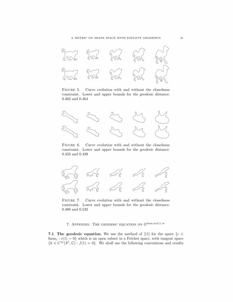
Figure 5. Curve evolution with and without the closednessconstraint. Lower and upper bounds for the geodesic distance:0.462 and 0.464
Figure 6. Curve evolution with and without the closednessconstraint. Lower and upper bounds for the geodesic distance:0.433 and 0.439
Figure 7. Curve evolution with and without the closednessconstraint. Lower and upper bounds for the geodesic distance:0.498 and 0.532
7. Appendix: The geodesic equation on Gimm,scal,1,∞
7.1. The geodesic equation. We use the method of [11] for the space {c ∈Immc : c(1) = 0} which is an open subset in a Frechet space, with tangent space{h ∈ C∞(S1,C) : f(1) = 0}. We shall use the following conventions and results
32 LAURENT YOUNES, PETER W. MICHOR, JAYANT SHAH, DAVID MUMFORD
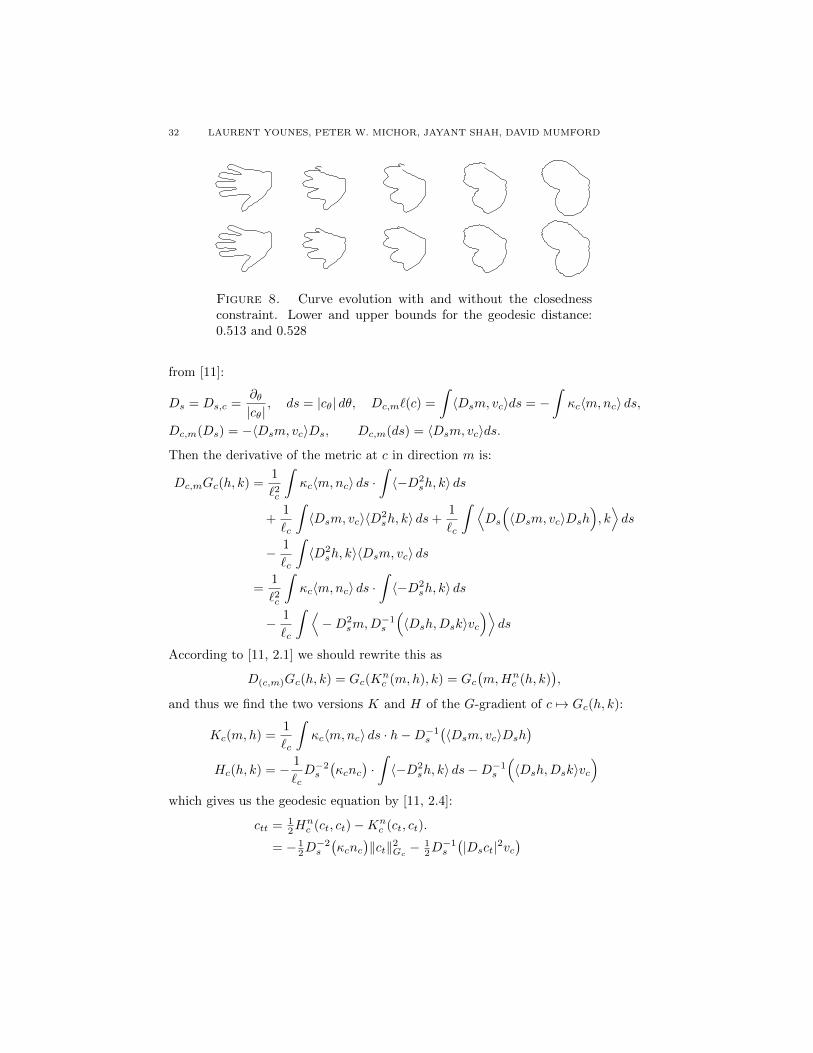
Figure 8. Curve evolution with and without the closednessconstraint. Lower and upper bounds for the geodesic distance:0.513 and 0.528
from [11]:
Ds = Ds,c =∂θ|cθ|
, ds = |cθ| dθ, Dc,m`(c) =
∫〈Dsm, vc〉ds = −
∫κc〈m,nc〉 ds,
Dc,m(Ds) = −〈Dsm, vc〉Ds, Dc,m(ds) = 〈Dsm, vc〉ds.
Then the derivative of the metric at c in direction m is:
Dc,mGc(h, k) =1
`2c
∫κc〈m,nc〉 ds ·
∫〈−D2
sh, k〉 ds
+1
`c
∫〈Dsm, vc〉〈D2
sh, k〉 ds+1
`c
∫ ⟨Ds
(〈Dsm, vc〉Dsh
), k⟩ds
− 1
`c
∫〈D2
sh, k〉〈Dsm, vc〉 ds
=1
`2c
∫κc〈m,nc〉 ds ·
∫〈−D2
sh, k〉 ds
− 1
`c
∫ ⟨−D2
sm,D−1s
(〈Dsh,Dsk〉vc
)⟩ds
According to [11, 2.1] we should rewrite this as
D(c,m)Gc(h, k) = Gc(Knc (m,h), k) = Gc
(m,Hn
c (h, k)),
and thus we find the two versions K and H of the G-gradient of c 7→ Gc(h, k):
Kc(m,h) =1
`c
∫κc〈m,nc〉 ds · h−D−1
s
(〈Dsm, vc〉Dsh
)Hc(h, k) = − 1
`cD−2s
(κcnc
)·∫〈−D2
sh, k〉 ds−D−1s
(〈Dsh,Dsk〉vc
)which gives us the geodesic equation by [11, 2.4]:
ctt = 12H
nc (ct, ct)−Kn
c (ct, ct).
= − 12D−2s
(κcnc
)‖ct‖2Gc −
12D−1s
(|Dsct|2vc
)

A METRIC ON SHAPE SPACE WITH EXPLICIT GEODESICS 33
− 1
`c
∫κc〈ct, nc〉 ds · ct −D−1
s
(〈Dsct, vc〉Dsct
)(23)
7.2. Theorem. For each k ≥ 3/2 the geodesic equation derived in 7.1 has uniquelocal solutions in the Sobolev space of Hk-immersions. The solutions depend C∞
on t and on the initial conditions c(0, . ) and ct(0, . ). The domain of existence(in t) is uniform in k and thus this also holds in Imm∗ := {c ∈ Imm(S1,R2) :c(1) = 0}.
Proof. The proof is very similar to the one of [11, 4.3]. We denote by ∗ any space ofbased loops (c(1) = 0). We consider the geodesic equation as the flow equation of asmooth (C∞) vector field on the H2-open set Uk×Hk
∗ (S1,R2) in the Sobolev spaceHk∗ (S1,R2)×Hk
∗ (S1,R2) where Uk = {c ∈ Hk∗ : |cθ| > 0} ⊂ Hk is H2-open. To see
that this works we will use the following facts: By the Sobolev inequality we havea bounded linear embedding Hk
∗ (S1,R2) ⊂ Cm∗ (S1,R2) if k > m+ 12 . The Sobolev
space Hk∗ (S1,R) is a Banach algebra under pointwise multiplication if k > 1
2 . For
any fixed smooth mapping f the mapping u 7→ f ◦u is smooth Hk∗ → Hk if k > 0.
We writeDs,c := Ds just for the remainder of this proof to stress the dependence onc. The mapping (c, u) 7→ −D2
s,cu is smooth U ×Hk∗ → Hk−2n and is a bibounded
linear isomorphism Hk∗ → Hk−2n
∗ for fixed c. This can be seen as follows (comparewith [11, 4.5]): It is true if c is parametrized by arclength (look at it in the spaceof Fourier coefficients). The index is invariant under continuous deformations ofelliptic operators of fixed degree, so the index of −D2
s is zero in general. But −D2s
is self-adjoint positive, so it is injective with vanishing index, thus surjective. Bythe open mapping theorem it is then bibounded. Moreover (c, w) 7→ (−D2
s)−1(w)
is smooth Uk×Hk−2n∗ → Hk
∗ (by the inverse function theorem on Banach spaces).The mapping (c, f) 7→ Dsf = 1
|cθ|∂θf is smooth Hk∗ × Hm
∗ ⊃ U × Hm∗ → Hm−1
for k ≥ m, and is linear in f . We have v = Ds,cc and n = iDs,cc. The mappingc 7→ κ(c) is smooth on the H2-open set {c : |cθ| > 0} ⊂ Hk
∗ into Hk−2∗ . Keeping
all this in mind we now write the geodesic equation (23) as follows:
ct = u =: X1(c, u)
ut = −D−2s,c
(12‖u|t=0‖2G.κc.nc + 1
2Ds,c(|Ds,cu|2.vc) +Ds,c(〈Ds,cu, vc〉.Ds,cu))
−( 1
`c
∫〈u,D2
s,cc〉 ds)∣∣∣t=0· u
=: X2(c, u)
Here we used that along any geodesic the norm ‖ct‖G and the scaling momentum− 1`c
∫〈ct, D2
s,cc〉 ds = ∂t log `(c) are both constant in t. Now a term by term
investigation shows that the expression in the brackets is smooth Uk×Hk → Hk−2
since k − 2 > 12 . The operator −D−2
s,c then takes it smoothly back to Hk. So the

34 LAURENT YOUNES, PETER W. MICHOR, JAYANT SHAH, DAVID MUMFORD
vector field X = (X1, X2) is smooth on Uk ×Hk. Thus the flow Flk exists on Hk
and is smooth in t and the initial conditions for fixed k.
Now we consider smooth initial conditions c0 = c(0, . ) and u0 = ct(0, . ) =
u(0, . ) in C∞(S1,R2). Suppose the trajectory Flkt (c0, u0) of X through theseintial conditions in Hk maximally exists for t ∈ (−ak, bk), and the trajectory
Flk+1t (c0, u0) in Hk+1 maximally exists for t ∈ (−ak+1, bk+1) with bk+1 < bk. By
uniqueness we have Flk+1t (c0, u0) = Flkt (c0, u0) for t ∈ (−ak+1,bk+1). We now
apply ∂θ to the equation ut = X2(c, u) = −D−2s,c ( . . . ), note that the commutator
[∂θ,−D−2s,c ] is a pseudo differential operator of order −2 again, and write w = ∂θu.
We obtain wt = ∂θut = −D−2s,c∂θ( . . . ) + [∂θ,−D−2
s,c ]( . . . ) + const.w. In the term
∂θ( . . . ) we consider now only the terms ∂3θu and rename them ∂2
θw. Then we get
an equation wt(t, θ) = X2(t, w(t, θ)) which is inhomogeneous bounded linear inw ∈ Hk with coefficients bounded linear operators on Hk which are C∞ functionsof c, u ∈ Hk. These we already know on the intervall (−ak, bk). This equationtherefore has a solution w(t, . ) for all t for which the coefficients exists, thus forall t ∈ (ak, bk). The limit limt↗bk+1
w(t, . ) exists in Hk and by continuity it
equals ∂θu in Hk at t = bk+1. Thus the Hk+1-flow was not maximal and can becontinued. So (−ak+1, bk+1) = (ak, bk). We can iterate this and conclude that theflow of X exists in
⋂m≥kH
m = C∞. �
References
[1] P. Alexandroff, H Hopf. Topologie. I. Springer-Verlag, Berlin-New York, 1974
[2] R. Basri, L. Costa, D. Geiger, and D. Jacobs, Determining the similarity of deformable
shapes, in IEEE Workshop on Physics based Modeling in Computer Vision, 1995, pp. 135–143.
[3] R.D. Benguriaand, M. Loss, Connection between the Lieb-Thirring conjecture for Schro-
dinger operators and an isoperimetric problem for ovals in the plane’, Contemporary Math.362 (2004), pp.53-61.
[4] M. P. Do Carmo, Riemannian Geometry Mathematical Theory and Applications, Birk-hauser, 1992.
[5] U. Grenander and D. M. Keenan, On the shape of plane images, Siam J. Appl. Math.,53 (1991), pp. 1072–1094.
[6] S. Helgason, Differential Geometry, Lie Groups and Symmetric Spaces, Graduate Studies
in Mathematics, Vol. 34, American Mathematical Society 1978 (revised version 2001).
[7] E. Klassen, A. Srivastava, W. Mio, and S. Joshi, Analysis of planar shapes using geodesicpaths on shape spaces, IEEE Trans. PAMI, (2002).
[8] A. Kriegl, M. Losik, P.W. Michor, Choosing roots of polynomials smoothly, II, Israel J.Math. 139 (2004), 183-188.
[9] A. Kriegl, P.W. Michor, The Convenient Setting of Global Analysis, Mathematical Sur-
veys and Monographs, Vol. 53, American Mathematical Society 1997.
[10] H. Krim and A. Yezzi, eds., Statistics and Analysis of Shapes, Birkhauser, 2006.[11] P. Michor and D. Mumford, An overview of the riemannian metrics on spaces of
curves using the hamiltonian approach, Applied and Computational Harmonic Analysis,doi:10.1016/j.acha.2006.07.004.

A METRIC ON SHAPE SPACE WITH EXPLICIT GEODESICS 35
[12] W. Mio, A. Srivastava, and S. Joshi, On the shape of plane elastic curves, tech. report,
Florida State University, 1995.
[13] Y. A. Neretin, On jordan angles and the triangle inequality in grassmann manifold, Ge-ometriae Dedicata, 86 (2001).
[14] B. O’Neill, The fundamental equations of a submersion, Michigan Math. J., (1966),
pp. 459–469.[15] E. Sharon and D. Mumford, 2d-shape analysis using conformal mapping, in Proceedings
IEEE Conference on Computer Vision and Pattern Recognition, 2004.
[16] A. Trouve and L. Younes, Diffeomorphic matching in 1d: designing and minimizingmatching functionals, in Proceedings of ECCV 2000, D. Vernon, ed., 2000.
[17] A. Trouve and L. Younes, On a class of optimal matching problems in 1 dimension, Siam
J. Control Opt., vol. 39, number 4, pp 1112-1135, 2001.[18] L. Younes, Computable elastic distances between shapes, SIAM J. Appl. Math, 58 (1998),
pp. 565–586.[19] L. Younes, Optimal matching between shapes via elastic deformations, Image and Vision
Computing, (1999).
Laurent Younes: Johns Hopkins University, Baltimore, MD 21218
E-mail address: [email protected]
Peter W. Michor: Fakultat fur Mathematik, Universitat Wien, Nordbergstrasse
15, A-1090 Wien, Austria; and: Erwin Schrodinger Institut fur Mathematische Physik,
Boltzmanngasse 9, A-1090 Wien, Austria
E-mail address: [email protected]
Jayant M. Shah: Northeastern University Department of Mathematics 360 Hunt-ington Avenue, Boston, MA 02115, USA
E-mail address: [email protected]
David Mumford: Division of Applied Mathematics, Brown University, Box F, Prov-
idence, RI 02912, USA
E-mail address: David [email protected]
Related Documents