A methodology to estimate renewal time scales in estuaries: the Tagus Estuary case

Frank Braunschweig Æ Flavio Martins

Paulo Chambel Æ Ramiro Neves

A methodology to estimate renewal time scales in estuaries:the Tagus Estuary case

Received: 4 November 2002 /Accepted: 2 June 2003� Springer-Verlag 2003

Abstract High-resolution hydrodynamic models are acommon tool to simulate water dynamics in estuaries.Results from these models are, however, difficult tointerpret without the aid of additional parametersto integrate the information. In this paper a methodologyto understand the transport patterns in the Tagus Estu-ary is proposed. It is based on the computation of tworenewal time scales: residence time and integrated waterfraction. This last parameter is used to build a depen-dency matrix that gives the integrated influence of eachregion of the estuary at a selected point. The parametersare computed using a Lagrangian transport model cou-pled to the hydrodynamic model. Results show thatTagus Estuary has two different types of regions: thecentral part of the estuary, with low renewal efficiency,and three regions with higher renewal efficiency. Renewalmechanisms are, however, different for each region asshown by the dependency matrix. Comparison of re-newal time scales with results from a water-quality modelrevealed that residence time is not a limiting parameterfor primary production in the Tagus Estuary.

Keywords Residence times Æ Renewal time scales ÆEstuary modeling Æ Tagus Estuary Æ Mohid model ÆHydrodynamic model Æ Lagrangian model

1 Introduction

Transit times, residence times and other renewal timescales have long been used as classification parametersfor estuaries and other semi-enclosed water bodies (Dyer1973; Bolin and Rodhe 1973; Zimmerman 1976; Take-oka 1984). The common objective of these parameters isto quantify the time that water remains inside an estu-ary. These time scales can be used as indicators to assessthe transport of substances inside an estuary. In thisway, general conclusions can be drawn regardingpollution dispersal, sediment transport or ecologicalprocesses in an estuary. From the ecological point ofview, for example, estuaries with a short transit time willexport nutrients from upstream sources more rapidlythan estuaries with longer transit times. On the otherhand, the domain average residence time – average res-idence time of water parcels inside the estuary – deter-mines if microalgae can stay long enough to generate abloom. In fact, estuaries with residence times shorterthan the doubling time of algae cells will inhibit for-mation of algae blooms (Kierstead and Slobodkin 1953;Lucas et al. 1999; EPA 2001). As a consequence, estu-aries with short residence time are expected to havemuch lower algae blooms than estuaries with longerresidence times. Renewal time scales also characterizethe exchanges between the water column and the sedi-ment: deposition of particulate matter and associatedadsorbed species depends on the particles’ settlingvelocity, water depth and particle residence time. This isparticularly important for the fine fractions with lowersinking velocities.

The different renewal time scales can thus be used togenerally characterize an estuary, to compare differentestuaries in respect to the transport processes, or

Ocean Dynamics (2003) 53: 137–145DOI 10.1007/s10236-003-0040-0

Responsible Editor: Hans Burchard

F. Braunschweig (&)Instituto Superior Tecnico,Sala 363, Nucleo Central,Taguspark, 2780-920, Oeiras, Portugale-mail: [email protected]

F. MartinsCIMA-EST/UAlg., Campus da Penha,8000-117 Faro, Portugale-mail: [email protected]

P. ChambelInstituto Superior Tecnico, Sala 363, Nucleo Central,Taguspark, 2780-920, Oeiras, Portugale-mail: [email protected]

R. NevesInstituto Superior Tecnico, Sala 361,Nucleo Central, Taguspark, 2780-920, Oeiras, Portugale-mail: [email protected]

to aggregate field data in easy-to-use parameters.Numerical models produce large amounts of informa-tion that must be processed and classified to becomeamenable to interpretation. Renewal time scales with ahigh spatial and temporal resolution can be used toaggregate and summarize information produced bynumerical models. The main questions are: which are thebest renewal time scales to characterize each process,and how to compute them? A large number of differentmethods have been proposed, ranging from simpleintegral estuary-wide formulas to more complex meth-odologies (Geyer 1997; Miller and McPherson 1991;Hagy et al. 2000). These methods attempt to account foradvection and mixing inside the estuary using indirectmeasurements such as freshwater flows and/or tracerconcentrations. They are usually applied to the wholeestuary or to a few areas of it. These methods are usefulto classify an estuary in a general way or to compile fielddata, giving a picture of the estuary’s transport. Sincethey possess a very low spatial and temporal resolutionand they lack an accurate description of the dynamics ofthe water masses, they cannot be used for detailedconsiderations.

In another type of approach, several methods wereproposed, using high-resolution hydrodynamic models,to simulate explicitly the transport processes. The con-cept of water age is one of these methods (Delhez et al.1999; Hirst 2000; Beckers et al. 2001). Deleersnijderet al. (2001) show that this concept can be generallyapplied to a constituent with any age characteristic (likeradioactive tracers, for example). In the case of the wateritself, the tracer age concentration is unitary. The water-age calculation reduces in that case to a standardadvection diffusion equation that can be solved with aEulerian or Lagrangian formulation. The Eulerian for-mulation can produce a high-resolution picture of thewater-age distribution over the entire domain. Fromthese results, global and local renewal time scales can becomputed. One advantage of the Eulerian approach isthat the same equations and numerical methods are usedboth for the hydrodynamic model and to transportwater constituents. With this approach it is, however,difficult to label water masses and relate their positionsin any instant of time with their release points. That taskis easily accomplished in Lagrangian models becauseparticles can carry information about their origin. Sev-eral authors have used Lagrangian implementations ofthe age concept (Tartinville et al. 1997; Oliveira andBaptista 1997), but usually the memory characteristic ofthe Lagrangian tracers is not explored. One problem ofthe Lagrangian approach is that the renewal time scalesare difficult to define in an unequivocal way. Residencetime of a region, for example, is usually calculated as thetime elapsed until all the water of that region (corre-sponding to all the tracers released at instant zero) isreplaced by new water. This criterion can lead to veryhigh residence times. For practical applications, theresidence is considered complete when a small amountof residual water is still in the region. The residual water

is usually defined in a subjective way as a certain fractionof the original water mass. Tartinville et al. (1997) showthat this problem can be overcome considering that thewater mass evolution in the region follows the expo-nential law:

mðtÞ ¼ mð0Þ expð�t=sÞ : ð1ÞThe residence time can thus be determined by adjustingan exponential regression to the model results anddefining s as the residence time. It must be noted thatthis assumption is valid only if the region is of a diffusivetype, in the sense defined by Deleersnijder et al. (1998).If the flux of tracer entering the region is constant overtime, the tracer mass will behave as Eq. (1) when theoutgoing flux is proportional to the mass of tracer inthe region. If the advective processes are important, theoutgoing flux is related to the ingoing flux by a delaytime. For the regions considered here the input flux isnot constant in time, since the output from one region isthe input to the adjacent ones. All regions have alsosome advective nature in the sense described above.Inspecting the tracer evolution in time it can, however,be seen that it decreases following approximately anexponential law, allowing the use of Eq. (1).

In this paper the characteristic time s is used toquantify residence times in the Tagus Estuary. An inte-grated renewal time scale, the integrated water fraction,is also used to understand the history of renewal in eachregion. Results were obtained using the MOHID prim-itive equation hydrodynamic model (Martins et al.2001), coupled to its Lagrangian transport module.Since the Lagrangian tracers can carry explicitly theinformation of its origin, this property is used to build adependency matrix that helps to understand the fate ofwater masses inside the estuary. Residence times andwater history are then interpreted together. As statedabove, renewal time scales can be an important indicatorof water quality and largely affect biological processes.The renewal parameters are compared with these eco-logical results to assess the importance of transport inthe biological processes of the Tagus Estuary.

2 Renewal time scales

In this study two different physical parameters aredefined: the residence time and the integrated waterfraction. These parameters are applied separately todifferent regions of the estuary. For this purpose, theestuary was divided into ten boxes where the high res-olution model results are integrated. It must be notedthat these boxes are used only for monitoring purposesand no box model was applied. Each box covers a givenarea and is composed of several cells of the underlyinggrid. The boxes are used in two functionalities: (1) torelease Lagrangian tracers and (2) to examine theLagrangian tracers which pass through them. A differentset of boxes can be used for each of these functions but,in order to simplify the result analysis in this paper, the

138

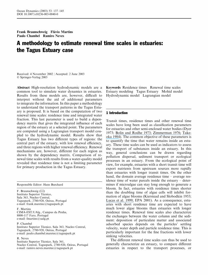
same set of boxes was used for the two purposes. Theboxes were placed in such a way as to fulfill the wholeestuary. Figure 1 shows their configuration. The numberand location of the boxes was based on prior knowledgeof physical and biological characteristics of the estuary.Boxes 3, 4 and 8 are placed over tidal flats, boxes 1, 2, 5,6 and 7 are located in the main channel, box 9 covers theSorraia channel and box 10 is located in the coastal re-gion, near the mouth, in the region of influence of theestuary plume.

Using the monitoring boxes, together with thememory property of the Lagrangian tracers, it is possibleto answer several important questions related to thewater-renewal process inside the estuary: (1) In whichareas are the water masses initially released in box i lo-cated? (2) From which areas did the water masses thatoccupy box i come at a certain instant? (3) What are themass fluxes between areas? In the next sectionsthe water-renewal parameters applied to these boxes arepresented.

2.1 Residence time

The first renewal time scale analyzed is the box’s averageresidence time. This parameter is defined as the timeneeded until the water volume initially in a given regionis replaced by new water. This can be applied to theestuary as a whole or to a single box.

Using the Lagrangian approach, this parameter canbe computed releasing an amount of tracers with avolume equal to the entire water body. The water frac-tion inside box i in each instant of time, with origin frombox j ( fi,j) is calculated as:

fi;jðtÞ ¼Vi;jðtÞVi;ið0Þ

; ð2Þ

where Vi,j(t) is the volume of tracers emitted in box j,present inside box i at time t and Vi,i(0) represents thewater volume in box i at the beginning of the simulation.For the especial case i ¼ j the average residence time fora given box can be computed. When Vii(t) reaches zero,all the box’s water is renewed and the box’s averageresidence time is found. In some regions a residualfraction of particles tends to stay inside the box for along time. Consequently, Vii(t) approaches zero veryslowly. This definition of residence time would then leadto excessively high values. An expedite way of solvingthis problem is to use a limiting residual fraction belowwhich the box is considered completely renewed. This,however, brings some subjectivity in the choice of theresidual fraction. In this article an alternative approachwas chosen using the method proposed by Tartinvilleet al. (1997). In this method results are adjusted toEq. (1) using an exponential regression. The residencetime is obtained as the value of s in that equation,without the need of any subjective parameter.

The application of the residence-time parameter todifferent boxes instead of using it for the whole estuaryincreases the spatial resolution of the analysis, but doesnot account for the interaction between boxes over time.The next parameter, integrated water fractions, can givethat information.

2.2 Integrated water fraction

The integrated water fraction, F, is obtained byintegrating the water fraction defined by Eq. (2) andnormalizing it by time:

Fi;jðT Þ ¼1

T

ZT

0

Vi;jðtÞVi;ið0Þ

dt : ð3Þ

Fig. 1 Division of the estuaryinto boxes

139

The parameter Fi,j measures the integrated influencefrom box j over box i during the time T. For the specialcase i ¼ j this parameter is related to the residence time.In this case, if the water inside the estuary were notrenewed at all, F would be equal to 1. As the water isrenewed inside a box, the contribution of the initialwater for the total volume of the box decreases and Ftends to 0. The time required until F ¼ 0 is thus anotherunequivocal way of computing the box’s residence time.The basic difference between these two methods ofcomputing residence times is that F keeps track of therenewal history of the box. The first method described inthis section was, however, preferred, since it produces avalue with an easier physical interpretation. On the otherhand, considering i „ j, F is a good parameter for rela-tive comparisons between boxes. In this case, the valueof F gives the integrated influence of box j over box i.Comparing the relative contribution of all boxes over i, aclear picture of water dynamics over time can beobtained. In this article the integrated water fractions Fwere used to build a matrix of dependencies betweenboxes.

3 Numerical model

3.1 General considerations

The numerical model used in the present study is theMOHID water-modelling system. It uses a full 3-Dformulation with hydrostatic and the Boussinesqapproximations (Miranda et al. 2000; Martins et al.2001). For the turbulent closure, the general ocean tur-bulence model, GOTM is used (Burchard et al. 1999). Inthis work the model is used with only one layer,behaving as a 2-D depth-integrated model. This is jus-tified by the estuary shallowness. Previous runs have

shown that 3-D effects are present only close to themouth and during high flow periods. Two transportmodels are coupled to this hydrodynamic module usingEulerian and Lagrangian formulations, respectively. Azero dimensional water-quality model is coupled to thetwo transport models. Interactions between the surfaceand the water column (e.g. heat fluxes, wind stress) arehandled by the surface module and the interactionbetween the bottom and the water column (e.g. oxygensinks, bottom friction) by the bottom module. Riverdischarges are imposed explicitly.

3.2 Model implementation

For the present study a horizontal grid of the ArakawaC type, with variable spacing between 1500 and 300 m,was used. The grid covers an area of 90 by 76 km.Figure 2 shows a zoom of the refined grid for the estuaryzone.

The Tagus Estuary is a meso-tidal estuary, withspring and neap tide amplitudes of 1.5 and 0.6 m,respectively. The Tagus River modal average monthlyflow is rather constant from March to December withan average value of 330 m3 s)1. From January toMarch higher values are recorded. The wind blowspredominantly from south and southwest during win-ter, rotating progressively to northwest and northduring spring and maintaining this direction duringsummer.

The hydrodynamic model was forced, imposing tidegauge elevations at the open boundary and using themean river discharges of the Tagus River (330 m3 s)1).The influence of wind over the renewal process was alsostudied. Two scenarios were used, one with no windforcing and other with a constant south wind of10 m s)1. The differences between the results were,

Fig. 2 Tagus Estuary bathyme-try and grid. Grid lines for therefined grid are shown

140

however, small, as shown in Fig. 5. For this reason onlythe results with no wind are analyzed. In the verticaldirection, only one layer was used to reduce computa-tional effort. Thus, 2-D depth-integrated results areobtained.

4 Results

4.1 General considerations

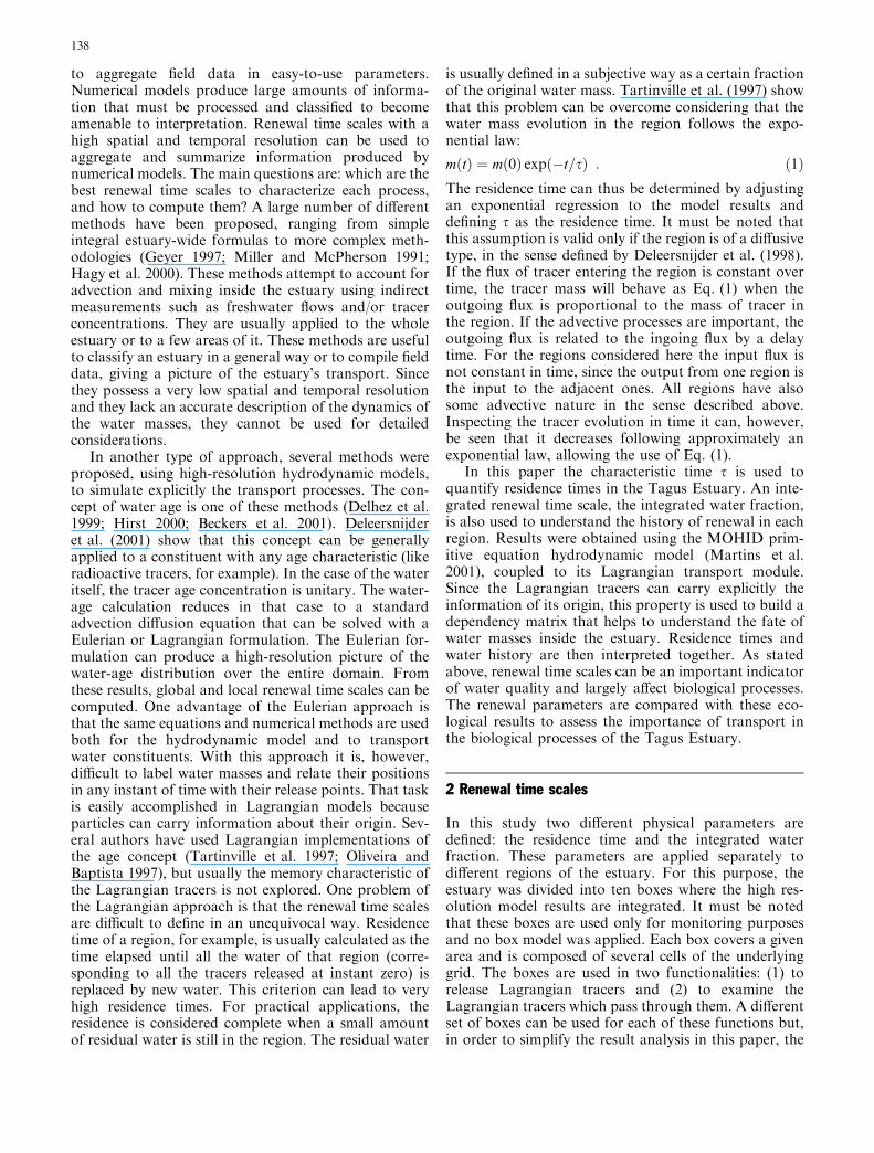
For the Tagus Estuary, 30 days’ runs were used tocompute the renewal time scales. The evolution of thewater volume inside the estuary during this period canbe observed in Fig. 3. An important fact is that the tidalprism, during neap tide, is about 25% of the mean watervolume and, during spring tide, about 40%.

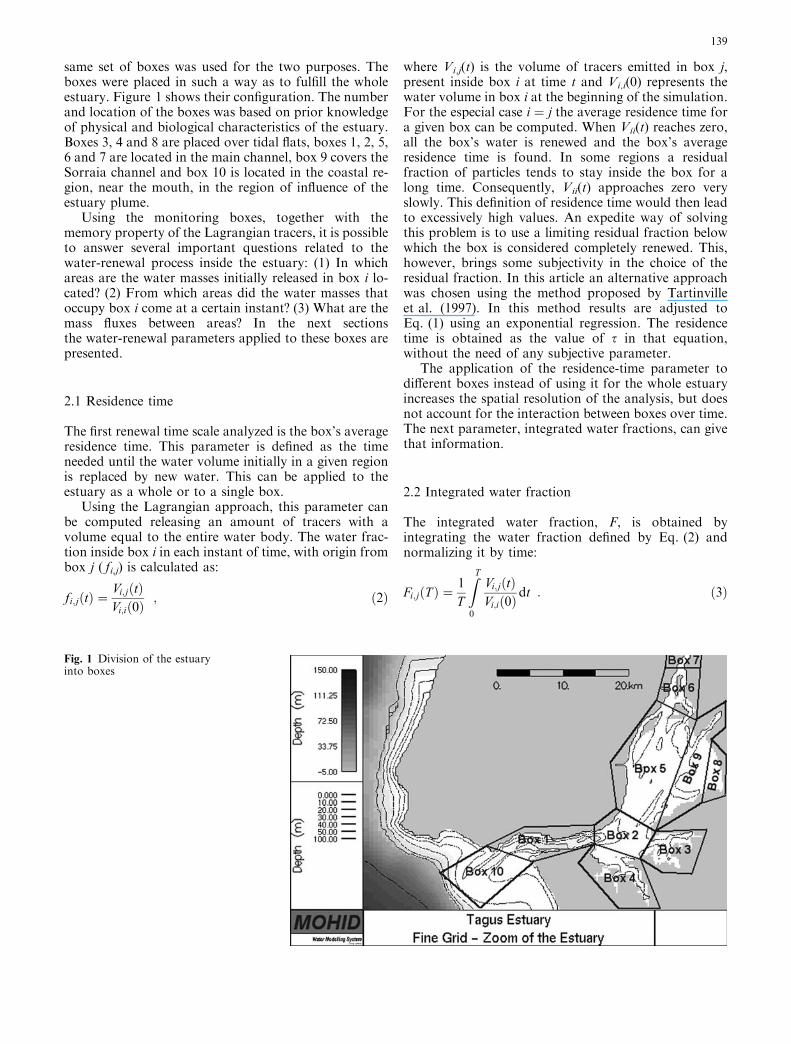
Taking into consideration the tidal prism, one canexpect a quick renewal of the water inside the estuary(considering the water from the open sea as freshwater),but some of the water which is flushed out of the estuaryduring ebb is ‘‘flushed in’’ again during flood, increasingthe residence time. The residual circulation at the TagusEstuary mouth helps to understand the water dynamicsof that region. Figure 4 shows the residual water flux(residual velocity multiplied by depth) at the mouth.Eddies observed in Fig. 4 show clearly that water flu-shed out through the main channel is transported backto the estuary, along the shores.

4.2 Residence times

In the present study all simulations started at high tideand in a transient period from neap tide to spring tide.The water fraction is first used to calculate the residencetime of the estuary as a whole. Figure 5 shows theevolution of the water fraction for the whole Tagus

Estuary for two scenarios: (1) no wind imposed and (2) aconstant south wind with 10 m s)1. This figure shows aslight difference between the two scenarios. The globalresidence times are, however, very similar: around25 days. From the analysis of the boxes it was concludedthat the tracers initially located near to the estuarymouth are removed more quickly from the estuary inscenario (2), but tracers initially located in the upperpart of the estuary stay inside the estuary for longertimes. Since the differences are only slight, only the no-wind scenario is used hereafter.

The residence times were then computed for each boxrepresented in Fig. 1. In the present paper two differentboxes (6 and 8) are used to explain the methodology.These two boxes have distinct natures: box 6 is locatedin the upper part of the estuary, characterized by rela-tively deep channels, where the freshwater influence inthe renewal process is high. Box 8 is located in a shallowarea away from the main channel. The renewal param-eters must be able to identify these differences. Figure 6shows the evolution of the water fraction f(t) for boxes 6and 8. In box 6 the water fraction decreases to almost

Fig. 3 Volume variation inside the Tagus Estuary during thesimulated period

Fig. 4 Residual water flux ofthe Tagus Estuary mouth

141

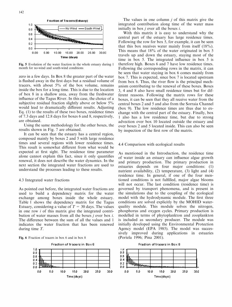
zero in a few days. In Box 8 the greater part of the wateris flushed away in the first days but a residual volume oftracers, with about 5% of the box volume, remainsinside the box for a long time. This is due to the locationof box 8 in a shallow area, away from the freshwaterinfluence of the Tagus River. In this case, the choice of asubjective residual fraction slightly above or below 5%would lead to dramatically different results. AdjustingEq. (1) to the results of these two boxes, residence timesof 7.3 days and 12.8 days for boxes 6 and 8, respectively,are obtained.

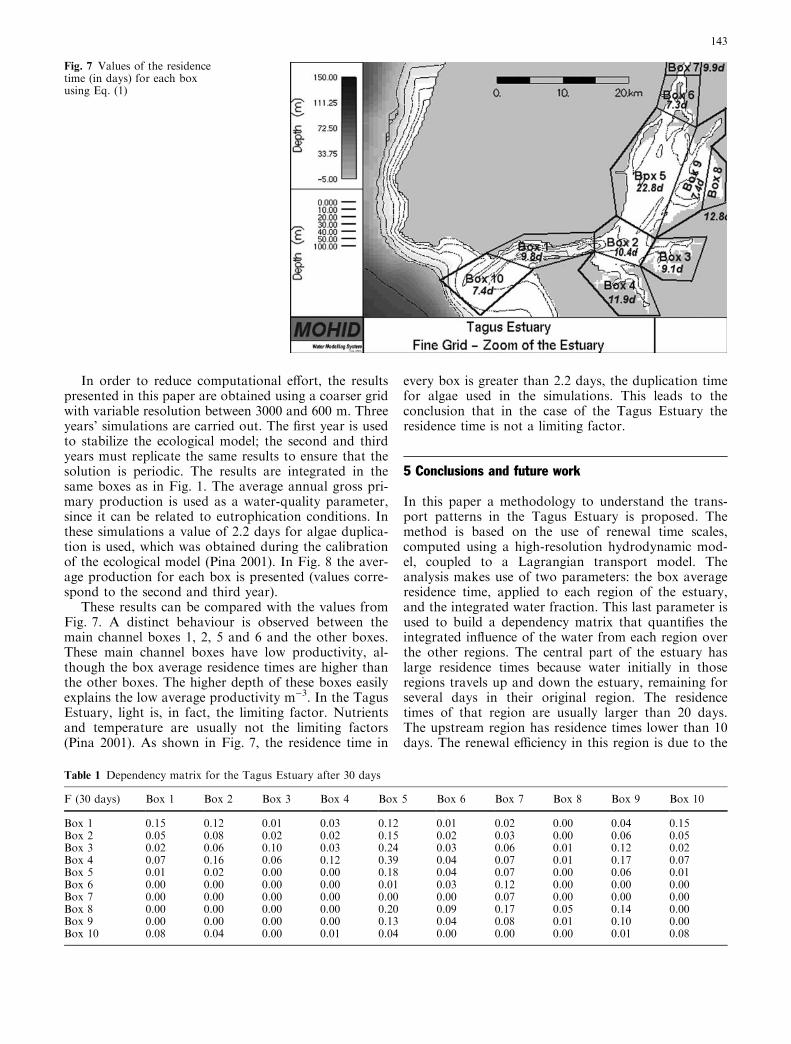
Using the same methodology for the other boxes, theresults shown in Fig. 7 are obtained.

It can be seen that the estuary has a central region,composed mainly by boxes 2 and 5 with large residencetimes and several regions with lower residence times.This result is somewhat different from what would beexpected at first sight. The residence time parameteralone cannot explain this fact, since it only quantifiesrenewal, it does not describe the water dynamics. In thenext section the integrated water fractions are used tounderstand the processes leading to these results.

4.3 Integrated water fractions

As pointed out before, the integrated water fractions areused to build a dependency matrix for the waterexchange among boxes inside the whole estuary.Table 1 shows the dependency matrix for the TagusEstuary, considering a value of T = 30 days. The valuesin one row i of this matrix give the integrated contri-bution of water masses from all the boxes j over box i.The difference between the sum of all the values and 1indicates the water fraction that has been renewedduring time T.

The values in one column j of this matrix give theintegrated contribution along time of the water massinitially in box j over all the boxes i.

With this matrix it is easy to understand why thecentral part of the estuary has large residence times.Following the row for box 5, for example, it can be seenthat this box receives water mainly from itself (18%).This means that 18% of the water originated in box 5travels up and down the estuary, staying most of thetime in box 5. The integrated influence in box 5 istherefore high. Boxes 6 and 7 have low residence times.Following the corresponding rows in the matrix, it canbe seen that water staying in box 6 comes mainly frombox 7. This is expected, since box 7 is located upstreamfrom box 6. Thus, the river flow is the principal mech-anism contributing to the renewal of these boxes. Boxes3, 4 and 8 also have small residence times but for dif-ferent reasons. Following the matrix rows for theseboxes, it can be seen that they all receive water from thecentral boxes 2 and 5 and also from the Sorraia Channel(box 9). The low residence times are thus due to ex-change with the central part of the estuary. Finally, box1 also has a low residence time, but due to strongadvection over box 10 located outside the estuary andover boxes 2 and 5 located inside. This can also be seenby inspection of the first row of the matrix.

4.4 Comparison with ecological results

As mentioned in the Introduction, the residence timeof water inside an estuary can influence algae growthand primary production. The primary production inestuaries depends on four major conditions: (1)nutrient availability, (2) temperature, (3) light and (4)residence time. In general, if one of the four men-tioned conditions is not fulfilled, major algae bloomswill not occur. The last condition (residence time) isgoverned by transport phenomena, and is present inthe simulations due to the coupling of the ecologicalmodel with the hydrodynamic module. The first threeconditions are solved explicitly by the MOHID water-quality module. This module solves the nitrogen,phosphorus and oxygen cycles. Primary production ismodelled in terms of phytoplankton and zooplanktonis included as secondary producer. The module wasinitially developed using the Environmental ProtectionAgency model (EPA 1985). The model was succes-sively improved during applications in estuaries(Portela 1996; Pina 2001).

Fig. 5 Evolution of the water fraction in the whole estuary during 1month for no-wind and south-wind conditions

Fig. 6 Fraction of tracers in box 6 and in box 8

142

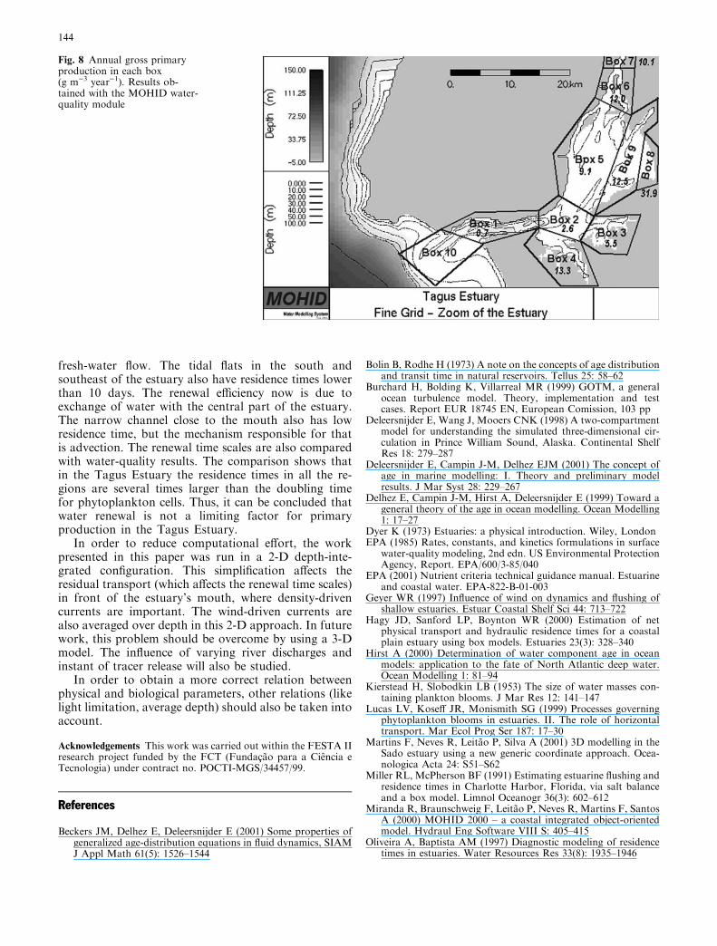
In order to reduce computational effort, the resultspresented in this paper are obtained using a coarser gridwith variable resolution between 3000 and 600 m. Threeyears’ simulations are carried out. The first year is usedto stabilize the ecological model; the second and thirdyears must replicate the same results to ensure that thesolution is periodic. The results are integrated in thesame boxes as in Fig. 1. The average annual gross pri-mary production is used as a water-quality parameter,since it can be related to eutrophication conditions. Inthese simulations a value of 2.2 days for algae duplica-tion is used, which was obtained during the calibrationof the ecological model (Pina 2001). In Fig. 8 the aver-age production for each box is presented (values corre-spond to the second and third year).

These results can be compared with the values fromFig. 7. A distinct behaviour is observed between themain channel boxes 1, 2, 5 and 6 and the other boxes.These main channel boxes have low productivity, al-though the box average residence times are higher thanthe other boxes. The higher depth of these boxes easilyexplains the low average productivity m)3. In the TagusEstuary, light is, in fact, the limiting factor. Nutrientsand temperature are usually not the limiting factors(Pina 2001). As shown in Fig. 7, the residence time in

every box is greater than 2.2 days, the duplication timefor algae used in the simulations. This leads to theconclusion that in the case of the Tagus Estuary theresidence time is not a limiting factor.

5 Conclusions and future work

In this paper a methodology to understand the trans-port patterns in the Tagus Estuary is proposed. Themethod is based on the use of renewal time scales,computed using a high-resolution hydrodynamic mod-el, coupled to a Lagrangian transport model. Theanalysis makes use of two parameters: the box averageresidence time, applied to each region of the estuary,and the integrated water fraction. This last parameter isused to build a dependency matrix that quantifies theintegrated influence of the water from each region overthe other regions. The central part of the estuary haslarge residence times because water initially in thoseregions travels up and down the estuary, remaining forseveral days in their original region. The residencetimes of that region are usually larger than 20 days.The upstream region has residence times lower than 10days. The renewal efficiency in this region is due to the

Table 1 Dependency matrix for the Tagus Estuary after 30 days

F (30 days) Box 1 Box 2 Box 3 Box 4 Box 5 Box 6 Box 7 Box 8 Box 9 Box 10

Box 1 0.15 0.12 0.01 0.03 0.12 0.01 0.02 0.00 0.04 0.15Box 2 0.05 0.08 0.02 0.02 0.15 0.02 0.03 0.00 0.06 0.05Box 3 0.02 0.06 0.10 0.03 0.24 0.03 0.06 0.01 0.12 0.02Box 4 0.07 0.16 0.06 0.12 0.39 0.04 0.07 0.01 0.17 0.07Box 5 0.01 0.02 0.00 0.00 0.18 0.04 0.07 0.00 0.06 0.01Box 6 0.00 0.00 0.00 0.00 0.01 0.03 0.12 0.00 0.00 0.00Box 7 0.00 0.00 0.00 0.00 0.00 0.00 0.07 0.00 0.00 0.00Box 8 0.00 0.00 0.00 0.00 0.20 0.09 0.17 0.05 0.14 0.00Box 9 0.00 0.00 0.00 0.00 0.13 0.04 0.08 0.01 0.10 0.00Box 10 0.08 0.04 0.00 0.01 0.04 0.00 0.00 0.00 0.01 0.08

Fig. 7 Values of the residencetime (in days) for each boxusing Eq. (1)

143

fresh-water flow. The tidal flats in the south andsoutheast of the estuary also have residence times lowerthan 10 days. The renewal efficiency now is due toexchange of water with the central part of the estuary.The narrow channel close to the mouth also has lowresidence time, but the mechanism responsible for thatis advection. The renewal time scales are also comparedwith water-quality results. The comparison shows thatin the Tagus Estuary the residence times in all the re-gions are several times larger than the doubling timefor phytoplankton cells. Thus, it can be concluded thatwater renewal is not a limiting factor for primaryproduction in the Tagus Estuary.

In order to reduce computational effort, the workpresented in this paper was run in a 2-D depth-inte-grated configuration. This simplification affects theresidual transport (which affects the renewal time scales)in front of the estuary’s mouth, where density-drivencurrents are important. The wind-driven currents arealso averaged over depth in this 2-D approach. In futurework, this problem should be overcome by using a 3-Dmodel. The influence of varying river discharges andinstant of tracer release will also be studied.

In order to obtain a more correct relation betweenphysical and biological parameters, other relations (likelight limitation, average depth) should also be taken intoaccount.

Acknowledgements This work was carried out within the FESTA IIresearch project funded by the FCT (Fundacao para a Ciencia eTecnologia) under contract no. POCTI-MGS/34457/99.

References

Beckers JM, Delhez E, Deleersnijder E (2001) Some properties ofgeneralized age-distribution equations in fluid dynamics, SIAMJ Appl Math 61(5): 1526–1544

Bolin B, Rodhe H (1973) A note on the concepts of age distributionand transit time in natural reservoirs. Tellus 25: 58–62

Burchard H, Bolding K, Villarreal MR (1999) GOTM, a generalocean turbulence model. Theory, implementation and testcases. Report EUR 18745 EN, European Comission, 103 pp

Deleersnijder E, Wang J, Mooers CNK (1998) A two-compartmentmodel for understanding the simulated three-dimensional cir-culation in Prince William Sound, Alaska. Continental ShelfRes 18: 279–287

Deleersnijder E, Campin J-M, Delhez EJM (2001) The concept ofage in marine modelling: I. Theory and preliminary modelresults. J Mar Syst 28: 229–267

Delhez E, Campin J-M, Hirst A, Deleersnijder E (1999) Toward ageneral theory of the age in ocean modelling. Ocean Modelling1: 17–27

Dyer K (1973) Estuaries: a physical introduction. Wiley, LondonEPA (1985) Rates, constants, and kinetics formulations in surface

water-quality modeling, 2nd edn. US Environmental ProtectionAgency, Report. EPA/600/3-85/040

EPA (2001) Nutrient criteria technical guidance manual. Estuarineand coastal water. EPA-822-B-01-003

Geyer WR (1997) Influence of wind on dynamics and flushing ofshallow estuaries. Estuar Coastal Shelf Sci 44: 713–722

Hagy JD, Sanford LP, Boynton WR (2000) Estimation of netphysical transport and hydraulic residence times for a coastalplain estuary using box models. Estuaries 23(3): 328–340

Hirst A (2000) Determination of water component age in oceanmodels: application to the fate of North Atlantic deep water.Ocean Modelling 1: 81–94

Kierstead H, Slobodkin LB (1953) The size of water masses con-taining plankton blooms. J Mar Res 12: 141–147

Lucas LV, Koseff JR, Monismith SG (1999) Processes governingphytoplankton blooms in estuaries. II. The role of horizontaltransport. Mar Ecol Prog Ser 187: 17–30

Martins F, Neves R, Leitao P, Silva A (2001) 3D modelling in theSado estuary using a new generic coordinate approach. Ocea-nologica Acta 24: S51–S62

Miller RL, McPherson BF (1991) Estimating estuarine flushing andresidence times in Charlotte Harbor, Florida, via salt balanceand a box model. Limnol Oceanogr 36(3): 602–612

Miranda R, Braunschweig F, Leitao P, Neves R, Martins F, SantosA (2000) MOHID 2000 – a coastal integrated object-orientedmodel. Hydraul Eng Software VIII S: 405–415

Oliveira A, Baptista AM (1997) Diagnostic modeling of residencetimes in estuaries. Water Resources Res 33(8): 1935–1946

Fig. 8 Annual gross primaryproduction in each box(g m)3 year)1). Results ob-tained with the MOHID water-quality module

144

Pina PMN (2001) An integrated approach to study the TagusEstuary water quality. Masters Thesis, Technical University ofLisbon

Portela L (1996) Modelacao matematica de processos hid-rodinamicos e de qualidade da agua no Estuario do Tejo (InPortuguese). Ph. D. Thesis, Technical University of Lisbon.

Takeoka H (1984) Fundamental concepts of exchange and trans-port time scales in a coastal sea. Continental Shelf Res 3: 311–326

Tartinville B, Deleersnijder E, Rancher J (1997) The water resi-dence time in the Mururoa atoll lagoon: sensitivity analysis of athree-dimensional model. Coral Reefs 16: 193–203

Zimmerman JTF (1976) Mixing and flushing of tidal embaymentsin the western Dutch Wadden Sea, part I. Distribution ofsalinity and calculation of mixing time scales. Netherlands J SeaRes 10(2): 149–191

145