A METHODOLOGY FOR SELECTING OPTIMAL COMPONENTS FOR SOLAR …

Solar Energy. Vol. 17. pp. 245-254. Pergamon Press 1975. Prinled in Orea! Britain

A METHODOLOGY FOR SELECTING OPTIMAL COMPONENTS FOR SOLAR THERMAL ENERGY

SYSTEMS: APPLICATION TO POWER GENERATION*

WILLIAM S. D UFF Solar Energy Applications Laboratory and Department of Mechanical Engineering, Colorado State Universi ty ,

St. Collins, CO 80521. U.S.A.

(Received 8 July 1974: in revised form 23 April 1975)

Abstract-A methodology is presented for determ ining the minimum-cost design for a solar thermal energy system. This approach builds up the minimum-cost system by add ing one subsystem at a time until the de ired system has been ynthesized. At each tep in the optimization procedure the intermediate system could be appl ied to an appropriate end use to find the mi nimum-cost design for that sy tern . For example, a min imum-cost solar furnace could be designed.

Thi systems optimization approach has two principal advantages over approaches that have traditionall y been u ed for solar thermal energy ystem . First, a vastly greater number of design can be con idered , and second , simplification of cost and performance models is not required. Co t and performance models may be in any form including tables or equations that must be solved implicitly.

An example of the systems optimization of the concentrator and absorber-heat exchanger subsystems is included, and the application of this approach to power generation is discussed.

INTRODUCTION

This paper presents a methodology for finding minimum-cost designs for solar thermal energy systems. This is a synthesis rather than an analysis approach , and it is an alternative to traditional engineering approaches used in the determination of optimum ystem designs. In this synthesis approach a system is built up in stages and at each stage a minimum cost design is determined for a large number of different specified performance . At each subsequent stage the system comes closer to being completed, and when the procedure is fini shed , the minimum cost system ha been determined. This ap-proach has been successfully used to analyze many other kinds of complex interrelated system , and it is believed that th is is the first time it has been applied to solar thermal energy system s.

One trad itional approach is to model the entire system in a simplified manner. This enables the experimentor to optim ize the system by direct search or by graphical means since there are now only a few design parameters. Since most design parameters are fixed, only a few of the multitude of possibilities can be examined. In fixing most of the des ign variables, only an extremely small fraction of the possible designs are examined and the system 's optimum is likely to be missed. Alternatively more design variables could be included. However, this red uces or negates the usefulness of direct search.

Two problems arise when direct search is used to find an optimum in a system with many design variable . First , direct search becomes extremely ineffective if there are more than two or three design variables, Wilde [I]. This is

*This paper was presented at the International Solar Energy Society's U.S. Sect ion Meeting held in Fort Collins, Colorado (Aug. 1974).

245

characterized by Bellman [2) as the curse of dimensional-ity. Second, di.reel search may not find an optimum when there are two or more design variable even if the response surface i . unimodal, Wilde [I]. Palmquist and Beckman [3) have demonstrated that there are multiple optima in rad iative-conducti ve systems. This makes the situation even wor e for direct search since "such systems have not been studied with any success ," Wilde[!]. Optimization using imulation is necessarily limited by these considerations.

Selcuk and Ward [4] in a recent article empl oyed mathematic models of cost and performance to analyze the collection of solar energy and its conversion to electricity. The optimization was by direct search. This approach , though simplified cost model s were used, recognized the need to view the co t per unit of output as the primary criterion for optimization. This more complex problem, however, required a performance analysis that omitted many potentiall y important design variables, such as concentrator rim angle. Thus, only a limited number of systems design variations could be examined.

Another approach that has been widely used in optim izing solar power generation systems i to fi x several point designs and then perturb design variables un til a systems optimum is converged upon. The non-linear programming based techniques that are used permit more design variables to be considered than in direct search, but these techniques are still drawn to local optima (see Palmquist and Beckman [3] for examples of this happen-ing in radiative-conductive sy terns.) Since multiple optima undoubtably exist in solar thermal energy systems, there is no assurance that a global optimum has been reached.

The dynamic programming based methodology, Bellman [2), described in this paper synthe izes or build

246 WILLIAM S. D UFF

up the solar thermal energy system in stages. At each stage you need consider only a few of the many design variables. Thus at each stage optimum systems are easily found.

A set of optimum concentrators indexed by properties of concentrated radiation they produce is found in the first stage. In the second stage , the absorber-heat exchanger is added to the concentrator, now characterized concisely by properties of concentrated radiation. A set of optimum collectors indexed by the propenies of thermal power that they generate can then be found. These min imum-cost collectors can be th~n used to find field designs that provide thermal power with specified properties at minimum cost. This minimum-cost thermal power can then be applied to an end use such as electric power generation.

The prime requisite for using this approach is being able to find a concise parametric representation that conveys all of the performance information about the subsystems thus far put together. This permits a minimum cost to be associated with different values of the parameters so that optimization may be performed when the next subsystem is added. If this can not be done an optimum system can not be guaranteed.

As this procedure progresses , the set of minimum-cost subsystems that has been built up can be used at any intermediate stage. For instance, if we only went as far as the concentrator, we could appl y the analysis to finding minimum cost solar furnaces.

There are two major advantages to this approach. First, a vastly greater number of designs can be considered. This will be demonstrated below. Second, simplified performance and cost models are not required as is the case in some of the traditional approaches. Nonlinearities, discontinuities and eq uations that must be solved implicitly can be included and wi ll fit in with the methodology quite easily. The primary consideration involved in performance and cost modeling is that of keeping computation times short.

MINIMUM COST OF CONCENTRATED RADIATIO

The first subsystem to be examined is the concentrator: The concentrator is optimized parametrically by specify-ing the target shape, the type of focusing and two parameters E and g. These characteristics are sufficient to describe the propertie: of concentrated radiation supplied to the next subsystem. Minimum costs are then computed for fixed values of the parameters , the parameter values changed and the process repeated. Expressions (1) below indicate the functional dependence of these two perfor-mance parameters on the concentrator design variables .

E= E(p,." A,, )* ( I)

g = g(Oma" <r<1>, aA, A,,, concentrator type)!

• E = p.," A,, for two ax is tracking concentrators. tThis li st would also include the heliostat size in the power

tower concept.

These functional relations constitute the constraints in the optimization. That is, the values of E and g are fixed and designs are varied to find a minimum cost design.

Expressions for E and g have been derived in Duff and Lameiro [5] for point focusing concentrators having spherical or pancake targets and for line focusing concentrators having round or flat targets. In the case of point focusing devices , the distribution of radiation is exponential with parameter g. For line focusing devices the distribution is normal with mean zero and standard deviation g. The normal distribution form agrees with the conjecture and experimental results in Lof and Duffie [6] and the exponential form has been derived using two different approaches [5 , 7] and has been verified experimentally [8].

The development is general in the sense that any sort of point or line focusing device can be examined and the corresponding E and g generated. For exam ple , Fresnel lenses, Fresnel reflectors, paraboloids , parabolic troughs, cylindrical Fresnel lenses, multiple fl ats and the heliostat array-power tower concept can be treated .

The target design variable in point focusing is the area of the pancake or cavity opening or the cross sectional area of the sphere. In line focusing it is the width of the cav ity or diameter of the tube. Thus, the amount of radiation available to a target can be computed by IoE and the amount of radiation actually intercepted can then be determined by specifying g, the target shape and its size.

The optimization procedure for multiple mounted , quasi-paraboloid concentrators was implemented on a computer as shown in Fig. l. As this procedure is carried out, a minimum cost of achieving performance of a concentrator characterized by various E and g combina-tions is determined. To find a minimum cost design for each concentrator type, 15 x 3 x 16 or 720 different designs were considered for each E and g combination.

3.; -- . 7 ·32 34

E/9000, --- E/500 8

45°, --- • 115° 15

0 ·75, 0 ·85, 0 90 3

0 ffi 16

Fig. I.

•

A methodology for selecting optimal components for solar thermal energy systems 247

This procedure is repeated for 34 x 8 or 272 different E, g pairs. Thus there are 272 different parametric minimum cost concentrators determined . At this point in the analysis we could design a solar furnace by specifying a target shape and then looking at different E, g combina-tions and their associated minimum costs to find the cheapest design achieving the desired results.

Jn the figure it is shown that lei the minimum cost for a given E, g pair, is updated each time a new design is found that is superior to the previous designs examined. Though not shown in the diagram , the minimum cost design that yielded the E, g combination is also saved for future reference. Thus, when an E, g pair is determined to be optimum for a particular application, such as a IO MW solar thermal electric power plant, the concentrator design that resulted in this minimum cost E, g pair can be retrieved .

MINIMUM COST OF THERMAL POWER FROM A COLLECTOR

The next subsystem to be added as we build up the minimum-cost solar thermal energy system is the absorber-heat exchanger. With this addition the concen-trator becomes a solar collector. The collector is optimized parametrically by specifying insolation level and 3 parameters of collector thermal power output; the mass flow rate through the absorber-heat exchanger 1il and the absorber-heat exchanger inlet and outlet tempera-tures , T;" and T out · These 3 parameters are required to adequately describe the properties of thermal power supplied to subsequent subsystems. Minimum cost collector designs are then found for fixed values of the three parameters, the parameter values changed and the process repeated .

The performance parameters, T;", T ou t and m, are functionally dependent on the collector design parameters and are functionally interdependent as well. Again, these functional relationships are the constraints in the optimization.

In the concentrator optimization the properties of concentrated radiation were expressed in two parameters , E and g, and a minimum cost of concentrated radiation was found for each E and g combination. Only these variables and the target shape need be considered as the concentrator part of the collector optimization , since they account for all the information required about the concentrator, including cost.

The collector performance expression of this character-ization of the concentrator is shown in eqn (2)*.

Q,, = F'[IoEmG(g, a)- ULAL(T,,, -T. )] (2)

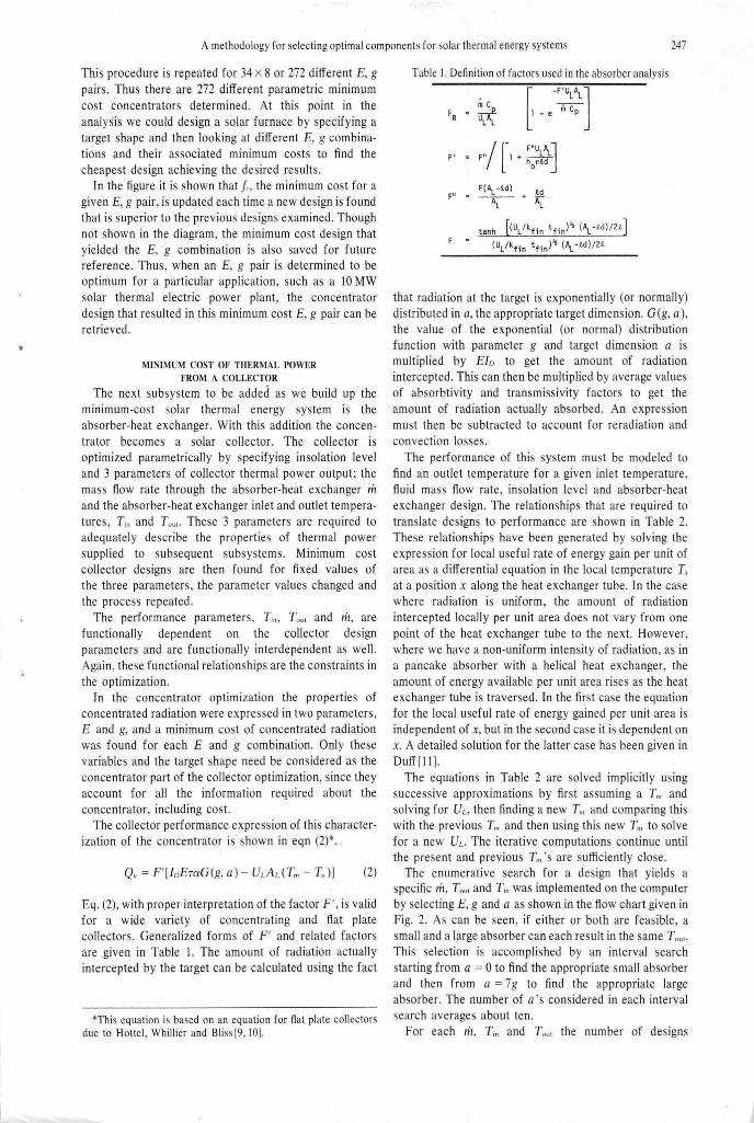
Eq. (2), with proper interpretation of the factor F ', is valid for a wide variety of concentrating and flat plate collectors. Generalized forms of F ' and related factors are given in Table I. The amount of radiation actually intercepted by the target can be calculated using the fact

*This equation is based on an equation fo r flat plate collectors due to Hottel , Whillier and Bliss[9, 10].

Table I. Definition of factors used in the absorber analysis

Fu =

F =

m c ~

r -F:UL\] l -e m Cp

F(\-i.d) id

~·AL

tanh ((ul / kfin tfin)~ (\ - i.d) /2l]

(UL/kfin tfin)~ (\ - i.d)/2 l

that radiation at the target is exponentially (or normally) distributed in a, the appropriate target dimension. G (g, a), the value of the exponential (or normal) distribution function with parameter g and target dimension a is multiplied by Elo to get the amount of radiation intercepted. This can then be multiplied by average values of absorbtivity and transmissivity factors to get the amount of radiation actually absorbed. An expression must then be subtracted to account for reradiation and convection losses.

The performance of this system must be modeled to find an outlet temperature for a given inlet temperature , fluid mass flow rate, insolation level and absorber-heat exchanger design. The relationships that are required to translate designs to performance are shown in Table 2. These relationships have been generated by solving the expression for local useful rate of energy gain per unit of area as a differential equation in the local temperature Tx at a position x along the heat exchanger tube. In the case where radiation is uniform, the amount of radiation intercepted locally per unit area does not vary from one point of the heat exchanger tube to the next. However, where we have a non-uniform intensity of radiation, as in a pancake absorber with a helical heat exchanger, the amount of energy available per unit area rises as the heat exchanger tube is traversed. In the first case the equation for the local useful rate of energy gained per unit area is independent of x, but in the second case it is dependent on x. A detailed solution for the latter case has been given in Duff[! I].

The equations in Table 2 are solved implicitly using successive approximations by first assuming a T,,, and solving for UL, then finding a new T,,, and comparing this with the previous T,,, and then using this new T,,, to solve for a new UL. The iterative computations continue until the present and previous T,,, 's are sufficiently close.

The enumerative search for a design that yields a specific rit, T out and T;., was implemented on the computer by selecting E, g and a as shown in the flow chart given in Fig. 2. As can be seen, if either or both are feasible, a small and a large absorber can each result in the same T out ·

This selection is accomplished by an interval search starting from a = 0 to find the appropriate small absorber and then from a = 7g to find the appropriate large absorber. The number of a 's considered in each interval search averages about ten.

For each rit, T;" and T out the number of designs


Table 2. Absorber performance equations DESCRIPTORS PANCAKE ABSORBER SPHERICAL FLAT LINEAR I CIRCULAR FLAT PLATE

ABSORBER ABSORBER LINEAR COLLECTOR ABSORB ER

L l Absorber Length a

G(g,a) l - e - 9 area under the (µ=0 o2=g) normal distribut ion l between -a/2 and +a/2

a area of circle cross sec ti ona 1 wi dth di amet er ---area of sphere

AL ( AL x - F'UL AL x) IoEL aTG(g ,a) c -F' ULALx)

F'I 0E aTe g egr - e rmc;;- iii1C - e P

T x F1 Ulg + nCP ULAL - F'ULALx -F ' ULAL x

+ (T. - T) e~+ T in a a + (\n - Ta) ermc;;- + T a

-~

[~(et-1)-~] F1I0E aTe g IoEL aTG(g,a) (1 - ~]

Tm F'ULg + m cp UL\

+ (Tin - Ta) FR + T + (Tin FR

rr a - Ta)p-+Ta

Qu F' [ !fl aT G( g, a) - ULAL(Tm - Ta)]

Note: 1. The equations for Tx and Tm in the second t hrough fifth columns and for Qu diffe r in form from those fou nd i n the literature. The form of the equat ions above is for the purpose of indi cat ing the s i mil ariti es of these equati ons with the equa t ions in the firs t column.

2. The flu id flow for the pancake absorber is t hrough a helical t ube and from the outs ide to t he cent er .

considered will be 272 x 2 = 544*. For each of the 544 designs the cost of the absorber-heat exchanger, including the cost of pumping power in the pipe, is computed and added to the minimum cost for concentrated radiation, fc(E, g), corresponding to that design's E and g. This total cost is the cost of the concentrator combined with the absorber-heat exchanger, that is, the cost of the collector. Out of these 544 designs the minimum-cost des ign is selected as the collector producing thermal power with the characteristics m, T out and T;. at minimum cost. This process is then repeated for I x I x 8 x 35 or 280 other values of m, T out and T; •.

Considerable savings in computation time has been achieved by synthesizing minimum-cost collectors in 2 stages rather than all at once. The maximum number of designs examined can be easil y seen fro m Figs. I and 2. The maximum number of de signs that are examined in the minimum cost of concentrated radiation analysis is 720 x 272 or 195,840 and 280 x 544 or 152,320 for the minimum cost of thermal power from the collector analysis. This is a total of 348, 160 des igns. If this was done in one step and the same number of designs were examined as were effectively examined in this case, we would examine 280 x 2 x 195,840 or 109,670,400 designs.

*Many times this num ber are actually considered since about JO candidate a 's are examined in the search procedure. In addition, other design variables such as absorber type, r, a, E, presence of a fi n, etc. are examined by rerunning the program with different settings. The design parameter d was set to achieve turbulent fl ow at as large a diameter as was feasible. It could also have been iterated over a set of values. Jn line focus ing an additional design variable, absorber length L, must also be considered. Seven values of L are run .

No. of values

1000 w/m2

40°C

0 ·005, ---. 1·0 kg/sec 8

150+, 200+,250 +, 300 +,350+°C 35

272

2

R.a+f (E,g) < ~(til, !,,,,, )

Yes

Fig. 2.

Another way of putting this is that by condensing the 195 ,840 concentrator designs into 272 a savings of about 300-1 in computational effort is achieved. This is possible since all of the characteris tics of concentrated radiation necessary for the absorber-heat exchanger analyses can be expressed in E and g without losing any potential minimu m cost collector des igns.

This economy is actuall y greater than indicated, as the flow chart onl y indicates the analysis of a particular type concentrator or absorber-heat exchanger. In reality all concentrator designs and types that did not result in minimum cost of concentra ted radiation having properties

•

A methodology for selec ting optimal component for solar thermal energy systems 249

E and g for a particular target shape would be eliminated. So if I 0 different types of concentrator are considered, then the information would be bei ng condensed from l ,958,400 total designs into 272 designs. The point here is that onl y the minimum cost designs need be retained. Thus, instead of 300-1 advantage there is now a 3000- l advantage.

As mentioned before, the performance and cost models can be arbitrarily complicated. The performance model s given in Table 2 are somewhat elaborate, but, if warranted , the y could be made more com plicated . This would , however, be at the expense of the computer time required to perform the analysis indicated in Fig. 2.

At this point in the analysis a set of minimum cost collectors has been buil t up by first examining the concentrator subsystem and then adding the absorber-heat exchanger subsystem. This set of minimum cost collectors is indexed by the different va lues of the parameters m, T," and Tou•· The set and its associated minimum costs can now be used to further build the system into a collector field delivering heat to a central point. The objective will be to determine the collectors, insulation thicknesses, pipe diameters, collector coupling and layouts that make up the minimum cost field s. Before doing this, some examples of collector optimization will be given.

EXAMPLES OF COLLECTOR OPTIMIZATION

Parametric cost fu nctions for various concentrators having pancake and spherical absorber-heat exchangers were developed as part of an NSF/RANN stud y[12]. These costs est imates were based on the assumption that the collectors would be manufactured on a large scale. Manufacturing plants would be et up, each capable of turning out 14,000 m' of collector aperture area per day. General des ign specifications were determined for each collector type and a comprehen ive range of potential state of the art manufacturing processes, materials and components were examined. Processes, materials and components that yielded different des ign performance characteristics, such as different pecular reflectivities, were identified. Noncompetitive processes , materials and components were then screened out on the basis of unit costs. An example of the output of this procedure for a parabolic concentrator is shown in Table 3 and Figs . 3 and 4. The figures provide adjustments to the cost es timates in the table for 3 design parameters: rim angle, aperture width and reflectivity . Parameterization of pointing and surface contour error was accomplished but is not illustrated. The costs of each of the other concentrator types were estimated in a similar parametric manner.

An example of part of the output from the minimum cost of concentrated rad iation analysis for Fresnel reflectors with pancake targets is shown in Table 4. The output under the minimum cost column is the set of values of fr. This analys is was repeated and similar tables generated for other point focusing concentrators deliver-ing radiation to a pancake target. Another set of analyses wa also performed on the same set of point focusing concentrators delivering radiation to a spherical target and on line focusing concentrators. After these analyses

Table 3. Itemized costs in $/m' of aperture area fo r minimum-costs 7·5 m diameter paraboloids with reflectivity of 85% and rim

angle of 80° Item

Install ed Cost, Without Absorbers

Materials

A 1 umi num she 11

Framing for shell

Gears and motors

Other

Labor and overhead to manufacture

Pipe suppor t

Foundation

Tracking mechanisms and controls

Transportation

Ins tallation of modules

Subtota 1

Contingency (5 percent)

TOTAL

18.50

1.20

4. 70

1.10

4 .90

6.40

6 .40

2.90

0.90

~

51 .oo _?_,§Q

53.60

-3·00 ~-~-~--~-~-~~-~-~ 45 55 65 75 85 95 105 115

Rim angle, "

Fig.3.

were completed the minimum costs for a particular E and g combination and target shape were compared. That is, all spherical target analyses were compared to determine the minimum cost types and designs of concentrators delivering radiation to that type of target. This minimum cost design was then carried into the second stage of the analysis-determining the minimum cost of thermal power fro m a collector.

Figure 5 is a graph of minimum cost for several types of point focus ing concentrators: a single mount paraboloid wi th a spherical target C 10 I (a pancake target, CIG3); a multiple array of long focus quasi-paraboloids with a common spherical target C3G2 (a pancake target. C3G4); a Fresnel lense with a spherical target C7G2 (a pancake target C7G4) and a Fresnel reflector with a spherical target C5G2 (a pancake target C5G4). As can be

250 WILLIA 1 S. DUFF

85 % Reflectivlly

-I 00 '---+---+-----1------+·

60 •1. Reflectivity

- 200 ~ Spin - formed (I 5 ml

~ Spin- formed (3·0 m i -3 00 Spin-formed (4·5 ml ..... H dro- drow

N ° -4 Q0~~~2~~2j~, l Spin- formed (6·0 m)

-500

-700 '---_..L--'----'---'----'---'----' 45 55 65 75 85 95 105 115

Rm 009le, •

Fig.4 .

Table 4. Minimum costs of concentrated radiation from Fresnel reflectors with pancake targets

PER MODULE cOsf FOR POINTING ANO SURFACE ACCURACY 1.0 PER SQUARE HETER COST FOR POINTING ANO SURFACE ACCURACY 1.0

----PARAMETERS---- -- ----------OPTllUH DESIGNS--- ------ -- HINIHUH EAP G N WP*SCOS* NW*TH RHO AP SIGMA COST

7 .04E+OO 7 .82£::04 7 .04E+OO 1 . lOE-03 7.04E+OO 1.53E-03 7.04E+oo 2.15E-03 7 .04E+OO 3.00E-03 7 .04E+OO 4.21E-03 7 .04E+OO 5.89E-03 7 .04E+OO 8.25E -03 7.39E+OO 8 .21E-04 7.39E+OO 1.15E-03 7 .39E+OO 1.61E-03 7.39E+OO 2.25E-03 7.39E+OO 3.16E-03 7 .39E+OO 4.42E-03 7.39E+OO 6.18E-03 7 .39E+OO 8.66E-03 7 .76E+OO 8.62E-04 7. 76E+OO 1. 21 E-03 7. 76E+OO 1.69E-03 7.76E+OO 2.37E-03 7. 76E+OO 3.31E-03 7 .76E+OO 4 .64E-03 7. 76E+OO 6. 49E-03 7 .76E+OO 9.90E-03 8.15E+OO 9.06E-04 8.15E+OO 1 .27E-03 8.15E+OO 1.77E-03 8.15E+OO 2.48E-03 8.15E+OO 3.48E-03 8.15E+OO 4.87E-03 8 .15E+OO 6.82E-03 8.15E+OO 9. 55E-03 8.56E+OO 9.51E-04 8. 56E+OO 1 .33E -03 8 . 56E+o0 1.86E-03 8.56E+OO 2.61E-03 8.56E+OO 3.65E-03 8. 56E+OO 5. llE-03 8.56E+OO 7.16E-03 8.56E+OO 1.00E-02 8.99E+OO 9.98£-04 8.99E+o0 1.40E-03 8.99£+00 1.96E-03 8.99E+OO 2.74E -03 8.99E+OO 3.84£-03 8.99E+OO 5.37E-03 8.99E+OO 7 .52E -03 8. 99E+OO 1 .05E-02 9.43E+OO l .05E-03 9. 43E+OO 1. 47E-03 9.43E+OO 2 .05E-03 9. 43E+OO 2. 88£-03 9 43E+OO 4.03E-03

.80

.80

.80

.80

. 80

.80

.80

.80

.80

.80

.80

.80

.80

.80

.80

.80

.80

.80

.80

.80

.80

.80

.80

.80

.80

.80

.80

. 80

.80

.80

.80

.80

.80

.80

.ao

.80

.ao

.ao

.80

.80

.80

.80

.ao

.80

.80

.80

.80

.80

.80

.80

.ao

.80

.80

1 30 .95 '.41£+00 .077 6.58£+04 1 40 .95 7 .41E+OO . 151 6 . 92E+02 1 35 .95 7 . 41E+OO .159 6 . 66E+o2 1 30 . 95 7.41E+OO .163 6.SOE+02 1 25 .95 7 . 41E+OO .160 6.38E+02 1 25 .95 7.41E+OO .196 6.37E+o2 1 25 . 95 7 . 41E+OO .237 6.36E+02 1 25 .95 7 . 41E+OO .284 6 . 35E+02 1 30 .95 7 .78E+OO . 077 6 .75E+04 1 40 .95 7.78E+OO . 151 7. 10E+02 1 35 • 95 7. 78E+OO . 159 6 .83E+02 1 30 .95 7.78E+OO . 163 6.67E+02 1 25 .95 7.78E+OO . 160 6.54E+02 1 25 .95 7.78E+OO .196 6.53E+02 1 25 • 95 7. 78E+OO . 237 6. 52E+o2 1 25 .95 7 .78E+OO . 284 6.51 E+02 1 30 .95 8 . 17E+OO .077 6.92E+04 1 40 .95 8.17E+OO .151 7 .27E+02 1 35 .95 8.17E+OO .159 7.00E+02 1 30 .95 8. 17E+OO .163 6.83E+02 125 .958.17E+OO .1606.70E+02 1 25 .95 8.17£+00 .196 6.69E+02 1 25 .95 8.17E+OO .237 6.68E+02 1 25 .95 8.17E+OO . 284 6.67E+02 1 30 . 95 8.58E+OO .077 7 .09E+04 1 40 .95 8.58E+OO .151 7 . 45E+D2 1 35 . 95 8.58E+OO .159 7.17E+02 1 30 . 95 8.58E+OO .163 6.99E+02 1 25 . 95 8.58E+OO .160 6.86E+02 1 25 .95 8.58E+OO . 196 6 .85E+02 1 25 .95 8.58E+OO . 237 6 .83E+02 1 25 .95 8.58E+OO .284 6 .83£+02 1 30 .95 9.0lE+OO .077 7 .25E+04 1 40 .95 9 .0lE+OO .151 7 .62E+D2 1 35 .95 9.0lE+DO .159 7.33E+02 1 30 .95 9.0lE+OO .163 7.16E+o2 1 25 .95 9.0lE+OO .160 7.02E+02 1 25 . 95 9 .0lE+OO .196 7.00E+02 1 25 .95 9.0lE+OO .237 6.99E+02 1 25 .95 9.0lE+OO .284 6.98E+02 1 30 .95 9.46E+QO .077 7 .41 E+04 1 40 .95 9.46E+OO .151 7.79E+02 1 35 . 95 9.46E+OO .159 7.49E+o2 1 30 .95 9.46E+OO .163 7.31E+02 1 25 . 95 9.46E+OO .160 7.17E+o2 1 25 . 95 9.46E+OO .196 7.16E+02 1 25 .95 9.46E+OO . 237 7.14E+02 1 25 .95 9. 46E+OO .284 7 . 13E+02 1 30 .95 9.93E+OO .077 7.57E+04 1 40 .95 9.93E+OO .151 7 . 95E+02 1 35 .95 9.93E+OO . 159 7.65E+02 1 30 .95 9 .93E+OO . 163 7.46E+02 1 25 .95 9 .93E+OO .160 7 .3ZE+02

*Used for the tower hel iostat analysis.

een the Fre nel reflectors dominate all other type for tbe range of E 's shown. This also hold true for other values of g. The co t for tbe two different target hape differed only lightly and thus appear a ingle line in the figure for each concentrator type. Thu the fc 's for Fresnel

2000 1----l---4--+---1--__;~L.,,.4,,~ -~1500 1----l---4--+--~~"7-I""'--+---+---! u

'iC'

i 1000 1---l---+~'4--_J,_-L-_.l.--'----1 '"" Quasi - paraboloid - single target

500 1---+---+-----+ Singly mounted paraboloids Circular Fresnel lenses Circular Fresnel reflectors

O'---_..L _ __1. __ .L__ ___ __. ______ __,

40 0 5 10 15 20 25 30 35

Effective aperture, m2

Fig. 5.

reflector were carried into the collector optimization for both pherical and pancake targets with other concen-trator types being eliminated.

The example next moves to the generation of minim um cost thermal power from a collector. The minimum cost of thermal power de igns for boiling collectors with pancake ab orber-heat exchanger for different value of 1i1 and TBOIL with J,> = IOOO w/m2 is shown in Table 5. An optimum design in Table 5 has had appended to it a reference or trace back to the concentrator that delivered minimum co t radiation for the E and g that was cho en as part of the minimum cost collector design. Thu the design of a minimum cost concentrator can now be specified. A graphic illu tration of this anal y i for several point focus collector types is shown in Fig. 6.

As a second example, the second part of the tower-helio tat optimization is shown in Table 6. Thi system i analyzed in the optimization procedure in a imilar manner to collectors. The performance analy i

differ omewhat though. For instance, the effective aperture is no longer imply the product of Av and P•••·

The fir t example illu trates the synthe is approach which ha been de cribed up to this point. To illustrate thi procedure in more detail , a specific design will be selected from Table 5, the collector in line I. Thi i a partial boil ing Fresnel reflector collector that produces a fl uid temperature of 150°C. The ma flow rate of thi collector i 0·040 kg/ ec, and the fraction of latent heat added i 0·075. The ab orber for thi collector i a pancake hape with a helical arrangement of tubes around the urface having a 0·020 m dia and length of 1 ·25 m. The

160 :;i:-

! 140

13 120 u ~ ., ~100 a.

~ BO :;; .c f- 60

40 0

~ J

Pressurised water o Pancake 160° o Poocoke 260° -x Cavity 160° <> Cavity 260° -

~- Partial steam ~' • Pancake 150° \.,_ o Cavity 260°

.o. Pancake 250" --~ ;::'~

fo• 1000 W/m2

---~ I I "'C>-1' l I

5 10 15 20 25 30 35 40 45 Thermo! power out, kW,

Fig. 6.

•


Table 5. Minimum costs of thermal power from concentrating collectors with pancake targets KFIN= 211. EPSIL0N- .90, ALPHA= .95, TAU= i.oo, fAMB- 26, FRACDL= 1.00 , VEL0CITY= 5.0, TYPE= 0, C~ST M0DEL= CAl

·--PARAMETERS- - - - - - - - - - - - - - - - -0PT I MUM DES I GNS- - - -- - - - - -- - - MIN !MUM TQBOIL QF MOOT D L LA AL G E C0ST ID= 1000 150 .075 .040 .020 1.25 150 .100 .040 .021 1 . 33 150 .035 . 080 .017 1 . 06 150 .050 .080 .021 1 . 32 150 .075 .080 .029 1.34 150 .1 00 . 080 . 033 2 .09 150 .013 . 160 .014 .85 150 .020 . 160 .022 1.37 150 .025 . 160 .028 1.75 150 .035 . 160 .035 2 . 22 150 .050 . 160 .033 2.09 150 . 075 . 160 .043 2.72 150 .010 . 320 .022 1 . 37 150 .015 .320 . 029 1.83 150 . 020 . 320 .032 2 .04 150 .025 .320 .033 2.09 150 .035 .320 .034 2.17 150 .005 .640 .022 1.37 150 .010 .640 .032 2.04 150 .015 .640 .038 2.39 150 .020 . 640 .050 3.17 200 .075 . 040 . 016 l .03 200 .100 . 040 .023 1.43 200 .033 .080 .015 .93 200 . 050 .080 . 023 1.43 200 .075 .080 .030 l .69 200 .100 .080 .030 2. 12 200 .015 . 160 .012 . 78 200 .020 . 160 .019 1.18 200 .025 .160 .023 l .43 200 . 035 . 160 .027 1.66 200 .050 .1 60 .034 2.12 200 .075 .160 .038 2.38 200 .100 .160 .052 3.24 200 .010 .320 .019 1.13 200 .015 .320 .023 l .43 200 .020 .320 .030 l . 87 200 .025 .320 .034 2 . 11 200 . 035 . 320 . 039 2 . 44 200 .050 .320 .051 3 . 22 200 . 005 .640 . 019 1. 13 200 .010 .640 .030 1 .87 200 .015 .640 .035 2. 19 200 .020 .640 . 040 2.49 200 .025 .640 .051 3.20 250 .075 .040 . 041 . 85 250 .100 .040 .021 1.27 250 .035 .080 .013 .79 250 .050 . 080 .021 1.27 250 .075 . 080 .026 1.57 250 .100 .080 .021 l.31 250 . 020 . 160 .015 .92 250 .025 . 160 .021 1.26 250 .035 .160 .023 1.43 250 .050 . 160 .027 1. 68 250 .075 . 160 .031 1.91 250 . 100 . 160 .035 2. 16 250 .010 .320 .015 .92 250 .015 .320 .025 1.54 250 .020 .320 .025 1. 72 250 .025 . 320 .027 1. 66 250 .035 .320 .029 1 . 79 250 .050 .320 .035 2. 16 250 .005 . 640 .015 .92 250 . 010 .640 .028 1.72 250 . 015 .640 .031 1 . 90 250 . 020 .640 .035 2.11 250 .025 .640 .035 2.16

2.525E -02 8 . 246E -03 7.040E+OO 6.350E+02 161 2 .819E -02 5.369E -03 8.985E+OO 7. 159E+02 164 l .804E -02 8 . 246E -03 7 .040E+OO 6.349E+02 156

l 2.785E-02 5.369E -03 8.985E+OO 7.159E+02 158 1 5. 402E -03 1.633E-02 1.394£+01 8.818E+02 161 l 6.961E-02 2. l88E -02 1. 868E+Ol 1. 086E+03 165 1 4.177E-02 8.246E-03 7.040E+OO 6.349E+02 153 l 2. 996E-02 8.658E-03 7.398E+OO 6.511E+02 154 l 4. 886 E-02 7 .517E-03 8 .985E+OO 7 . 145£+02 154 1 7 . 367E -02 1 . 481E-02 l .264E+Ol 8 . 227E+02 156 l 6.939E-02 2.l88E-02 1.868E+Ol l. 086£+03 158 1 1.l73E-01 3. 232E-02 2.760E+Ol 1.454E+03 162 l 2.990E -02 8 . 658E -03 7.392E+OO 6.511E+02 152 1 5.357 E-02 1.279E-02 l.092E+O l 7 .659E+02 153 l 6.643E -02 1 . 714E -02 l . 464E+Ol 9.125E+02 154 l 6.927E-02 2.l66E -02 1.868E+Ol 1.036E+03 155 1 7 .479E-02 l . 068E -02 2.503E+Ol 1 .355E+03 156 l 2.990E-02 8.658E-03 7.392£+00 6.513£+02 151 1 6.629£-02 1.714E-02 1.464E+Ol 9.125£+02 152 1 9.074E -02 1 .809E -02 2. 162E+Ol 1 .204£+03 153 1 l .591£- 01 3.394E-02 2.898£+01 1. 518E+03 154 1 1.717E-02 8.246E -03 7.040£+00 6.349E+02 209 l 3 . 328E- 02 l . 002E-02 8.557E+OO 6.986£+02 211 l l .395£-02 8.246£-03 7.040E+OO 6.349E+02 205 1 3 .31 2E-02 l .002E -02 8. 557£+00 6.986£+02 206 l 5.805E -02 1.481E-02 1.264E+Ol 8 . 232E+02 209 1 7 .302 E-02 1.984E-02 1.694£+01 1.0l5E+03 212 1 9.580E-03 8.246£-03 7 . 040£+00 6.349E+02 202 1 2.251E-02 8.246E -03 7.040£+00 6.350E+02 203 1 3.304E-02 1.002E-OJ 5.557£+00 6 .936£+02 203 1 4.468E-02 1.410E-02 1.204E+Ol 7 .946£+02 205 1 7 .256£-02 1.984£-02 1.694£+01 1. 015£+03 206 l 9. 146£-02 2.094£-02 2.503£+01 1 .349E+03 210 l 1.701E - 01 3.929E-02 3.355E+Ol 1.703E+03 212 l 2.251E-02 3.246E-03 7.040£+00 6. 331£+02 202 l 3.880E-02 5.920£-03 9 . 906E+OO 7. 453E+02 202 l 5 . 692E-02 1.111£-02 1. 327E+Ol 8.537 E+02 203 1 7.225E-02 1.984£-02 1.694£+01 1.015£+03 204 1 9. 653£-02 2. 792£-02 2. 384£+01 1. 294£+03 205 1 1.676£-01 3.929£-02 3.355£+01 1.703£+03 207 1 2.245E-02 3.246£ -03 7.040E+OO 6.354£+02 201 1 5 . 657£- 02 1.lllE- 02 1. 327£+01 8 .538E+02 202 1 7. 769£-02 2. 412£- 02 2. 059£+01 1. 163E+03 202 1 1.002E-01 3.232E-02 2 .760E+Ol 1.456E+03 203 1 1. 664E- 01 3.929E-02 3 . 255£+01 1.703E+03 204 1 1 .222£- 02 8.246£ -03 7 .040E+OO 6.850E+02 257 1 2. 744E -02 6.184£ -03 7 .392E+OO 6.527E+02 259 l l .052E-02 8.246E-03 7 .040E+OO 6.350E+02 254 l 2.725 £-02 6.184£-03 7.392E+OO 6.527£+02 255 l 4. l87E-02 1 . 343E -02 l . 147E+Ol 7 .820E+02 257 l 2 . 928E-02 6 . 247E -03 l .464E+Ol 9. l 93E+02 260 l 1.438£-02 8.246E -03 7.040£+00 6. 351E+02 252 1 2 . 706E-02 6.134E-03 7.392 E+OO 6 . 527E+02 253 1 3 . 454E-02 8. 702£-03 1.040E+Ol 7 .584E+02 254 1 4.81 0E-02 8.746E-03 l.464E+Ol 9 . l 80E+02 255 1 6.173£-02 l .900E-02 2 . 270E+Ol l . 248E+03 258 1 7.965£-02 2.546£-02 3 . 043£+01 1.579£+03 260 1 1 .437E-02 8.246E-03 7.040E+OO 6.353£+02 251 1 4.029£-02 1.052£-02 8. 985£+00 7 . l51E+02 252 1 5 .057£-02 1.410£-02 1.204£+01 7.963E+02 252 1 4 . 701£-02 8 . 746E- 03 1.464£+01 9.179E+02 253 1 5.461£-02 1.231E-02 2. 059£+01 1. 169E+03 254 1 7 .940E-02 2.546£-02 3.048£+01 1 .579£+03 256 l 1.437£-02 8 . 246E-03 7 .040£+00 6.362E+02 251 1 5.046£-02 1.410£-02 1.204£+01 7 .964£+02 251 1 6. l1 6E-02 1.488E-02 1.770£+01 1. 054£+03 252 1 7 . 588E-02 1.994E-02 2.364£+01 l .299£+03 253 l 7.925£ -02 2 .546E -02 3 . 043£+01 1.579E+03 253

parameter LA in this table is the absorber length and is used only for line focusing collectors. The parameter N is fo r the case where N individual absorbers are used for each concentrator in a multiple array. AL, the surface area of one side of the pancake absorber, is 0·02525 m2, E and g are 7·040 m2 and 0·008246 m2 respectively. The minimum cost for delivering heat with characteristics TBOIL of 255°C, QF of 0·075 and m of 0·040 kg/sec is $635 . The power out which can be calculated from TBOIL, QF and iii * is 6350 W. The concentrator design which was retained has been appended under the " trace back" heading. This information can also be found in Table 4. The concentrator providing concentrated radia-

*TBOIL, QF and 1i1 take the place of T0 "" T;" and 1i1 fo r the boiling analysis.

--- -----TRACE BACK- --- -- --N W CR NWTHRH0 AP SIGMA C. TYPE FC ETA $/ KW

293 336 411 340 272 282 629 260 194 169 283 247 260 215 232 234 352 260 232 251 192 432 271 531 272 229 244 750 329 273 284 246 288 208

l 329 1 313 1 246 l 247 l 260 1 211 l 330 l 247 1 279 1 290 1 212 1 606 1 284 1 705 1 286 1 288 l 526 1 515 1 288 1 317 l 320 l 387 l 402 1 516 l 285 l 251 1 328 1 397 1 403 1 516 1 251 1 306 1 331 1 1 404

ENO. 175 . 037

1 25 .95 7.41£+00 .284 C5G4 1 25 .95 9. 46£+00 . 196 C5G4 1 25 .95 7.41 £+00 .284 C5G4 l 25 .95 9.46£+00 .196 C5G4 1 25 . 95 1.47£+01 .234 C5G4 1 25 . 95 1 . 97£+01 .284 C5G4 1 25 .95 7.41E+OO .234 C5G4 1 25 .95 7.78£+00 .234 C5G4 1 25 . 95 9.46E+OO . 237 C5G4 1 25 . 95 1 . 33£+01 . 284 C5G4 1 25 . 95 1.97E+Ol . 284 C5G4 1 25 .95 2.91£+01 .284 C5G4 1 25 . 95 7. 78£+00 . 284 C5G4 1 25 .95 1.15E+Ol .284 C5G4 1 25 . 95 1. 54E+Ol .284 C5G4 1 25 . 95 1. 97£+01 . 284 C5G4 1 25 .95 2.63E+Ol . 160 C5G4 l 25 .95 7.78£+00 .254 C5G4 l 25 . 95 1 . 54£+01 . 254 C5G4 1 25 . 95 2 .28£+01 . 237 C5G4 1 25 .95 3 . 05£+01 .284 C5G4 1 25 .95 7. 41 £+00 .284 C5G4 l 25 . 95 9 . 01 E+OO .284 C5G4 l 25 .95 7 .41£+00 .284 C5G4 1 25 .95 9.01£+00 .284 C5G4 1 25 . 95 1.33£+01 .284 C5G4 1 25 . 95 1 .78£+01 . 284 C5G4 1 25 .95 7 .41E+OO .284 C5G4 1 25 . 95 7. 41 E+OO .284 C5G4 1 25 .95 9.0lE+OO .254 C5G4 1 25 . 95 1.27E+Ol .284 C5G4 1 25 . 95 1. 73E+Ol . 284 C5G4 1 25 .95 2 .63£+01 .237 C5G4 1 25 .95 3 . 53E+Ol .284 C5G4

25 .95 7.41E+OO .284 C5G4 25 . 95 1 .04E+Ol .196 C5G4 25 .95 1.40E+Ol .237 C5G4 25 . 95 1 .78E+Ol . 284 C5G4 25 .95 2.51E+Ol .284 C5G4 25 . 95 3. 53l+Ol . 284 C5G4 25 .95 7 .41E+OO .284 C5G4 25 .95 1.40E+Ol .237 C5G4 25 .95 2 .17E+Ol .284 C5G4

l 25 . 95 2 . 91E+Ol .284 C5G4 l 25 . 95 3. 53E+Ol . 284 C5G4 l 25 .95 7 .41E+OO .284 C5G4 l 25 . 95 7. 78E+OO . 237 C5G4 l 25 .95 7 .41E+OO . 284 C5G4 1 25 . 95 7. 78E+OO . 237 C5G4 1 25 .95 1.21£+01 .284 C5G4 1 25 .95 1.54E+Ol . 160 C5G4 1 25 .95 7.41E+OO .284 C5G4 1 25 .95 7.78E+OO .237 C5G4 1 25 .95 1.09E+Ol .237 C5G4 1 25 .95 1. 54E+Ol .196 C5G4 1 25 .95 2.39E+Ol .237 C5G4 l 25 .95 3.20E+Ol .237 C5G4 1 25 .95 7 .41E+OO . 284 C5G4 1 25 .95 9.46E+OO .284 C5G4 l 25 .95 1. 27E+Ol .284 C5G4 1 25 . 95 l .54E+Ol . 196 C5G4 1 25 . 95 2 .17E+Ol .196 C5G4 l 25 .95 3.20E+Ol .237 C5G4 l 25 .95 7.41E+OO .284 C5G4 l 25 . 95 l . 27E+Ol . 284 C5G4 l 25 .95 l .87E+Ol .237 C5G4 l 25 .95 2 .51E+Ol .237 C5G4 l 25 .95 3 . 20E+Ol .227 C5G4

1370.662 61324

6 .347£+02 .854 1. 00E+02 7. l 56E+02 . 892 8. 48E+Ol 6.347£+02 .797 1 .67E+02 7 .156£+02 .892 8.48E+Ol 8.503£+02 .863 6 . 96E+Ol l .085E+03 .858 6 .43E+Ol 6.347£+02 .680 1.25E+02 6.508£+02 .868 9.04£+01 7 .143£+02 .892 8.47E+Ol 8.219E+02 .889 6. 96E+Ol 1.085E+03 .859 6.43E+Ol 1.453£+03 .872 5.74£+01 6.508E+02 .868 9.64£+01 7 .683E+02 .831 7 . 59E+Ol 9.116£+02 .876 6 . 76E+Ol l .085£+03 .855 6.43£+01 1.354£+03 .897 5.73E+Ol 6 .508£+02 .868 9.63E+Ol 9.118£+02 .876 6. 76£+01 1.203E+03 .890 5.94E+Ol 1. 511 E+03 . 885 5 . 60£+01 6. 347E+02 . 784 1. 09E+02 6.980£+02 .859 9 .02£+01 6.347£+02 . 731 1. 17£+02 6.980£+02 .859 9.02E+Ol 8.219£+02 .873 7.09E+Ol 1.013£+03 .868 6.55E+Ol 6 . 347£+02 . 627 1. 37E+02 6.347£+02 .836 1.03E+02 6 .980E+02 .859 9.02E+Ol 7. 937£+02 . 855 7. 33£+01 1.013E+03 .863 6.55£+01 1 .346£+03 .881 5.81£+01 1.696£+03 .877 5 . 50E+Ol 6.347E+02 .836 1.03E+02 7 .447£+02 .891 8 . 02E+Ol 8.524£+02 .886 6.89£+01 1.013E+03 .868 6 .55£+01 1 . 292E+03 .864 5 . 97£+01 1.696£+03 .877 5.50E+Ol 6. 34 7£+02 . 836 1 . 03E+02 8.524E+02 .886 2 .89£+01 1.161E+03 .857 6 . 26£+01 1.453£+03 .853 5 .88£+01 l . 696E+03 . 877 5. 50£+01 6.347E+02 . 691 l .24E+02 6 .516E+02 .877 9.56£+01 6 . 347E+02 . 645 l. 33E+02 6 .516E+02 .877 9.56E+Ol 7 . 30QE+02 .848 7 .64E+Ol 9. l82E+02 .886 6. 73E+Ol 6.347E+02 . 737 1.16E+02 6 .516E+02 .877 9.56E+Ol 7.569£+02 .873 7.93E+Ol 9.155£+02 .886 6.72£+01 1. 244£+03 .857 6.09£+01 1. 574£+03 .853 5. 78£+01 6.347£+02 .737 1.16£+02 7.132E+02 .866 8.73£+01 7.937E+02 .862 7.29£+01 9.155£+02 .886 6. 72E+Ol 1.166E+02 .882 6.12£+01 l . 574£+03 .853 5.78£+01 6.347£+02 . 737 1.16£+02 7.937E+02 .862 7.29E+Ol l .051£+03 .875 6.48£+01 1.294E+02 .871 5.95E+Ol l .574£+03 .853 5.78£+01

tion with characteristics E and g at minimum cost is 7-4 1 m in aperture area with a rim angle of 25° and a surface coating having a reflectivity of 0·95. The combined tracking and surface contour accuracy is about 0·285°. The collector effi ciency of 85 ·4 per cent, the cost of thermal power of $100/kW and the concentration ratio Av/a of 295 are quantities that can now be found from informatio n m the table. They are also displayed for convenience.

MINIMUM COST OF THE HEAT FROM A COLLECTOR FIELD

The collector field is synthesized using the same dynamic programming principles as were used in synth-esizing the collector. The sub-system of the collector fi eld used in the synthesis analysis to build up the field consists of a collector (or collectors) and the associated heat


Table 6. Minim um costs of thermal power from tower-heli ostat systems B0 ILING HEAT TRANSFER VERSl~N KRIN= 211 , EPSIL0N= .90, ALPHA= .95, TAU= 1 .00, TAMB= 20 , FRACDL = 1.00, VEL~C ITY• 5.0, TYPE= I, C0ST M0DEL= CA9

PARAM ETERS ····---~PTIMUM DESIGNS······ MINIMUM TB~Il MD0T D l Al lOOG E/100 C0ST $/KW KW

IO= 1000 150 166 .0 .100 39079 3927 65534 6217 47464252 111 427347 150 169.3 .140 39181 5512 58193 5520 36568661 84 435894 150 172.6 .160 24940 4009 27429 5100 32784517 74 444441 150 176 . 0 .200 29563 5941 59356 5631 35833327 79 452988 150 179.3 .140 13142 1849 38407 7141 45731605 99 461535 150 182.6 .140 28433 4000 75278 7141 46631217 99 470082 150 185.9 .140 34931 4914 43245 57 43 38248366 80 478629 150 189.2 . 220 15874 3509 91764 8705 55159808 113 487176 150 192. 6 . 140 48664 6845 105390 71 41 48204238 97 495723 150 195 . 9 .140 13278 1868 45900 8534 54818548 109 504270 150 199 .2 .240 16468 3971 88200 8367 52995767 103 512816 200 169.3 .180 17019 3111 45892 6095 38801898 87 443623 200 172.6 .180 35123 6421 99311 6729 43300168 96 452321 200 176.0 .180 8890 1625 45900 8534 54117828 117 461020 200 179.3 .240 8330 2030 36916 6864 43449496 93 469718 200 182.6 .120 26078 3178 51682 6864 46406107 97 478417 200 189 . 2 .120 36076 4396 47746 6341 44723000 90 495814 200 192 .6 .140 17344 2466 36916 6864 44490334 88 504512 200 195. 9 . 220 26334 5884 45810 6217 39816661 78 513211 200 199.2 .160 37545 6101 73802 7001 45856624 88 521909 250 166.0 .240 12895 3218 44992 5975 38365632 88 435819 250 169. 3 .140 30389 4424 43245 5743 38076342 86 444535 250 172.6 .220 12860 2942 30284 5631 36103982 80 453251 250 176.0 .220 9309 2130 35482 6597 42033061 91 461968 250 179.3 .220 18292 4185 45892 6095 39326576 84 470684 250 192 .6 .220 13013 2977 60554 8042 51429898 102 505550 250 195.9 .240 8844 2207 41573 7730 49276189 96 514266 250 199.2 .180 17284 3235 60554 8042 51635575 99 522982

transport segment (or segments) that connects it to the collector (or collectors) next closest to the inside of the field . The field is synthesized from the outside to the in ide and each collection of subsystems of the fie ld is optimized over a range of T;., Tout and 1iz . A typical fi eld will branch from larger heat transport pipes on the inside to smaller heat transport pipes on the out ide. This branching structure is illustrated in Fig. 7. Computer programs have been set up to carry out the optimization for the main trunk and feeder lines for both steam and water. As can be seen in Fig. 7 the field can be constructed by starting with the feeder lines depicted at the top of the

(a) Feeder lines

(b) Main frunk lines

~ Sysfems Previously Synfhesized

D System to be added

Fig. 7.

········TRACE BACK ········ WP NW CR TH RH0 AP/100 TWR SIGMA FC/1000 ETA CONC.FILE

7 17907 1971 70 .90 19349 286 .432 39133 .221 09G2E 7 15901 1247 70 .90 17181 269 . 429 34735 .254 09G2E 7 14690 1584 70 .90 15873 259 .279 32089 .280 09G2E 7 16219 1180 70 .90 17525 272 .429 35431 .258 09G2E 7 20570 4809 70 . 90 22225 306 .291 44995 .208 09G2E 7 20570 2223 70 . 90 22225 306 .436 44992 . 212 09G2E 7 16544 1455 70 .90 17875 275 .351 36144 .268 09G2E 7 25075 3088 70 . 90 27093 338 .441 54958 .180 09G2E 7 20570 1299 70 . 90 22225 306 . 527 44990 . 223 09G2E 7 24583 5688 70 . 90 26561 335 .296 53870 . 190 09G2E 7 24101 2623 70 .90 26041 331 .440 52797 .197 09G2E 7 17556 2439 70 . 90 18969 283 .353 38364 .234 09G2E 7 19383 1305 70 .90 20943 297 .525 42376 .216 09G2E 7 24583 6538 70 . 90 26261 335 .296 53870 .174 09G2E 7 19771 4209 70 . 90 21362 300 .289 43234 .220 09G2E 7 19771 2689 70 .90 21362 300 .357 43233 . 224 09G2E 7 18265 1796 70 . 90 19735 288 .354 39920 .251 09G2E 7 19771 3465 70 .90 21362 300 .289 43234 .236 09G2E 7 17907 1315 70 .90 19349 296 .354 39134 .265 09G2E 7 20167 1429 70 .90 21790 303 .435 44103 .240 09G2E 7 17212 2312 70 .90 18597 280 .353 37609 .234 09G2E 7 16544 1616 70 .90 17875 275 .351 36144 .249 09G2E 7 16219 2383 70 .90 17525 272 .283 35434 . 259 09G2E 7 19003 3557 70 . 90 20533 294 .288 41544 .225 09G2E 7 17556 1813 70 .90 18969 283 .353 38364 .248 09G2E 7 26165 3863 70 .90 25029 325 .361 50726 .202 09G2E 7 22266 4360 70 . 90 24057 319 .293 48739 .214 09G2E 7 23165 3095 70 . 90 25029 325 .361 50726 .209 09G2E

END

3663. 742 I 22202 . 7741 ma§ figure and the n putting branches together into main trunk lines as illustrated at the bottom of the figure. By doing this, any kind of fi eld arrangement may be synthesized , that is, built up in stages from the outside of the field to the inside.

The optimization find s the minimum cost fi eld layout by varying collectors and the pipe sizes and insulation thickness on each subsystem in such a way as to achieve a field which provides thermal power with specified characteristics m, T;., Tout· The optimization is then repeated for other values of 1i1 , T;. and Tout· Series connections, single parallel connections, double parallel connections, higher order parallel connections and stag-gered parallel connections of collectors can all be accoun ted for in this approach. This particular approach allows for a more general design of field layout than other approaches because each subsystem is designed individu-all y. Thus, if there are economies that can be achieved by differentially insulating different subsystems or by having different pipe diameters for different subsystems, they will be recognized by the optimization.

Figure 8 is an illustration of the interaction between the high and low temperature sides for a parallel arrangement of collectors. It is intended to show the need to simultaneously consider both low and high temperature heat transport sides in the optimization. Thi is the case since, at each stage, the heat transport design affects the high and low side temperature profiles (the upper and lower curves in the figure) and therefore the outlet temperature of the collector and the high ide heat transport line where mixing occurs. Table 7 is an actual optimization run for pressurized water. It illustrates the high and low side temperature profiles for the minimum cost system and gives the corresponding optimum high and low side insulation thicknesses and pipe diameters for each heat transport segment.

At this point in the analysis optimum fields have been

•

..


--- 260°

~ ......... ~ --~~-_,_ _ _,. _ __. ____ -+- -- 250°

0 t; 2 0 u

High temperature side

__L--L---:-!:"-_,___.. ___ 175° I --~ """'rature side

~-- LCNI te .. ,...-

Fig.8.

Table 7. Sample resu lt for a pressurized water feeder line optimization run

FILE NAME ? T1S10S5 NEW EXPERIMENT ? ! 1<11X, 1<11XL,NMX,FTYPE,SM,TO,TRISE,Tll ,T!!L 111 ,61 ,10, .OS ,111, 111, l, .1S YD ,XO ,FNS ,FEW ,CC ? l,10.S,.S,.S,1SS4 QUE,Q JOB IN EXECUTION ACCUM. CPU SECONDS - 939. 4 72 TRACE BACK STAGE AND DESIGN T AND TL ? 10,100, 100 TRACE BACK FROM STATE 10 COST 41331 DESIGN T AND TL 100.00 100 .00 STAGE---HIGH SIDE OT, D, TI---LOW SIDE OT,D,TI 10 o. .023B .0319 .1S .0131 .0330 19 o. .0131 .0311 .1S .0113 .0400 18 0. .022S .032S .1S .0113 .0413 17 o. .0117 .0317 .1S .0103 .04SO 16 0. .0110 .0330 .1S .0191 .04S1 lS o. .0101 .0333 .1S .0181 .OS10 14 o. .019S .033S .1S .0170 .OS6S 13 0. .OlBI .0337 .1S .OlSI .0611 11 0. .0179 .0339 .1S .Ol4S .0694 11 o. .0170 .0340 .1S .0131 .0789 10 0. .0161 .0340 .1S .Olli .0919 9 o. .01S3 .0340 .2S .0102 .1106 B 0. .0143 .033B .2S .0080 .1180 7 o. .0131 .03S3 .so .0118 .040S 6 o. .0119 .0368 .so .0110 .0497 S 0. .0107 .03B3 .SO .0090 .06SS 4 0. .0093 .0398 .SO .OOBO .1174 3 1.00 .OOBO .1774 .IS .OOBO .0770 1 1.00 .0080 .07B6 1.00 .OOBO .109S l -s .oo .0080 .OISI 1.00 .0080 .1021

TRACE BACK STAGE AND DESIGN T AND TL ? 10,100, 100 TRACE BACK FROM STAGE 10 COST 19110 DESIGN T AND TL 200.00 100.00 STAGE- --HIGH SIDE OT, D, TI---LOW SIDE DT,0,Tl 10 D. .0174 .0241 .SO .0172 .0280 9 D. .0164 .0147 .SO .0168 .0313 8 0. .0164 .02S1 .SD .0143 .03S7 7 o. .0143 .02S6 .so .0127 .0411 6 D. .0131 .0160 .SO .OlOB .OS18 s 0. .0117 .02/S .IS .OllS .031S 4 l. 00 . OOBO . 0306 . IS . 0092 . 0422 3 1.00 .OOBO .0460 1.00 .0083 .0366 2 1.00 .0080 .0364 l .SO .OOBO .0340 l -6.00 .0030 .043S 2.SO .0080 .OS16

laid out and thermal power outputs of these fields with their associated minimum costs may be used for various end purposes. One end use could be to generate electricity and another could be to centrally supply heat for heating and cooling of build ings.

The next section wi ll treat a specific application for which this methodology was developed-generat ion of electrical power by solar thermal means.

APPLICATION TO POWER GENERATION

At this point minimum cost collector field layouts for various value of 1i1, T,, and T out have been determined . These outputs and their associated minimum costs can now be matched to a turbine-generator-heat rejection

SE Vol. 17, No. 4-D

system. To properly continue the synthesis methodology, a turbine should be designed for the field that takes into account the cost of heat associated with specified values of m T,,, T out· The costs of turbines of varying efficiencies and heat rejection systems of varying efficiencies are now added to the cost of the system synthesized so fa r- the concentrator, then the absorber-heat exchanger to make up the collector, and then the combination of collectors and their heat transport segments to make up the field-to arrive at a minimum cost per kWh solar thermal electric generation system. This is accomplished by utilizing a histogram of insolation levels that typifies daily insolation variation. Output from this optimization is hown in Table 8.

Table 8. Sample results when the turbine generator/cooling tower sub-system is added in the optimization

ELECT ST EAM !NL ENG FIELD TUR-GEN C00LING ELECT C 0 N 0 E N S E R APPR P0WER FL0W TMP EFF C0STS C0STS C0STS C0ST TEMP INL 0UT RNG THP ~:! 'GWl Rs& .84 ~i1!§ 1'?.h Wt! Sim 0

1gREn c~n~r0EJ 31.5 43 .4 2SO .84 282 . lB 92.46 27.97 .024 40 28 38 10 3 31.6 43.5 2SO .84 281. 72 92 . 44 27.97 .024 40 28 38 10 3 31.7 43 .6 250 .84 281.71 92.40 27.96 .024 40 28 38 10 3

110 .1 148. I 1SO .86 297 .DO 83 . 31 24 .1 5 .024 40 28 38 10 3 110.2 148 .2 250 .86 296.76 83.30 24.15 .024 40 28 38 10 3 110.4 148.5 250 .86 296 . 16 83.27 24. 14 .014 40 28 38 10 3 110.7 148.8 250 .86 296 .39 83.13 14.14 .024 40 2B 38 10 3 95 .3 147.8 200 .86 313 . 61 90.12 19.46 .026 40 28 38 10 3 95 .4 147.9 200 .86 313.38 90.11 29.46 .026 40 28 38 10 3 95.6 148 .2 200 .86 312.81 90.03 29. 46 .026 40 28 38 10 3 96.4 149 .5 200 .86 310.11 89.94 29.45 . 026 40 28 38 10 3 75.7 147.6 lSO .86 356 .59 104.45 40 .0l .030 40 28 38 10 3 7S.8 147.7 150 .86 356.3S 104 . 44 40.01 .030 40 28 38 10 3 75 .9 148 .0 150 .B6 355.75 104.41 40. 01 .030 40 28 38 10 3 76.0 148.3 lSO .86 355.08 104.38 40 . 01 .030 40 28 38 10 3 27.3 43.4 200 .84 294.84 98.95 33 .95 .026 40 28 38 10 3 27.4 43.4 200 .84 294.57 98 .93 33.95 .026 40 2B 38 10 3 27 .4 43.5 200 .84 294. 10 98.90 33.94 . 026 40 28 38 10 3 27.5 43.6 100 .84 194.08 98.86 33.93 .026 40 18 38 10 3 11.7 43 .4 lSO .84 345.96 112.37 45.BO .030 40 28 38 10 3 21.8 43.4 150 .84 346.10 112.35 45.79 .030 40 28 38 10 3 21.8 43.S 150 .84 345.55 11 2.32 45.79 .030 40 28 38 10 3 21.8 43.6 150 .84 345.21 112.28 45.77 .030 40 28 38 10 3

ext the possibility of storing some of the heat generated during the high insolation hours of the day was examined. The gain in util ization by discharging storage after usable sunshine hours have past and the lower cost of small turbine generators were traded off against the cost of obtaining this storage. This was accompl ished using an hour by hour dynamic simulat ion over the period of several years. The simulation also verified the kWh output pred icted by the optimization analysis.

OTHER APPLICATIONS AND EXTENSIONS

A major advantage of this synthes is type of approach is that each of the intermediate tage , such as the concentrator, are minimum-cost sy terns and th us they can be matched up with an appropriate end use of their outputs. In addition to the end use already mentioned, the techniques described in this paper may also be applied to supplying industrial heat or to the development of a small electric power generation plant coupled with one or two collectors.

Dynamic considerations can be accounted for in the optimization by conducting sensitivity analysis on the ambient conditions such as wind velocity and insolation level. The model wi ll eventuall y be extended to explicitly account for these dynamic considerations.

Acknowledge111e11t-The research on which this paper i based has been supported by the National Science Foundation RANN program under Grant G 1378 15.


REFERENCES I. D. J. Wilde. Optimum Seeking Methods. Prentice-Hal! ,

Englewood Cliffs, New Jersey (1964). 2. R. Bellman, Dynamic Programming. Princeton University

Press, Princeton, New Jersey (1957). 3. R. W. Palmquist and W. A. Beckman, Optimum thermal

design of radiative-conductive y terns. Trans. of the ASME: J. Engng Indust., May ( 1972).

4. M. K. Selcuk and G. T. Ward , Optimization of solar terrestial power production usi ng heat engines. Trans. of the ASME: Journal of Engineering for Power, April (1970).

5. W. S. Duff and G. F. Lameiro, A performance comparison method for solar concentrators. Submitted to Trans. of the ASME: Journal of Engineering for Power.

6. G. 0. G. Uif and J. A. Duffie , Optimization of focu ing solar collector design. Trans. of the ASME: Journal of Engineering for Power, Ju ly (1963).

7. G. Y. Umarov, Problems of olar energy concentration. Ge/iotekhnika 3 (5), (1967).

8. R. A. Zakhidov and D. I. Teplyakov, Power characteristics of solar reflecting devices under operative tracking conditions. Geliotekhnika 2 (5), (1966).

9. H. C. Hottel and A. Whillier, Evaluation of flat plate solar collector performance. Proc. Conf. on the Use of Solar Energy, II, Univ. of Arizona (1958).

10. R. W. Bliss Jr., The derivation of several 'plate efficiency fac tors ' u eful in the design of fl at plate solar heat collectors, Solar Energy 3 (1959).

I I. W. S. Duff. The analysis of the performance of a pancake absorber-heat exchanger for a solar co llector. Submitted to the Trans. of the ASM E: Journal of Engineering for Power.

12. Solar Thermal Power Systems, Final Report, Volume 3. NSF/RANN Grant G/-37815, Colorado State University Solar Energy Application Laboratory, Fort Collins, Col-orado, November (1974).

NOME 'CLA TURE

a absorber dimension (m' or m) AL area for losses of the absorber (m' or m'/m) A,, concentrator aperture (m' or m'/m) C,, fluid specific heat (w sec/kg°C) d absorber tube diameter (m) E effective concentrator aperture (m' or m'/m) f, minimum cost of concentrated radiation having

properties E and g ($) F' defined in Table 1 F. defined in Table 1

g measure of spread of concentrated radiation (m' or m'/m)

G distribution function with parameter g and variable a

ho fluid heat transfer coefficient (w/m'°C) / 0 direct component of solar radiation (w/m') k thermal conductivity (w/m' C) 1 absorber tube length (m)

L absorber length 1i1 mass flow rate (kg/sec) N number of individual reflector elements in a concen-

trator P ~"' power out (w)

Q. total useful energy rate (w) RA absorber cost for a given T, a, f , AL, Ta.,, d, 1, 1i1 , L

and absorber heat exchanger type ($) R, concentrator cost for a given p •• ., A,,, Omaxo O',, O';,

concentrator type combination ($) thickness

T. ambient temperature (0C) T,. absorber inlet temperature (°C)

To.. absorber outlet temperature (' C) Tm absorber average temperature (°C) T, temperature at x (°C) UL heat loss coefficient for the absorber (w/m''C)

x distance along heat exchanger tube from the inlet (m) a ab orbtivity of the absorber f emissivity of the absorber

Pm average reflectivity (or transmis ivity) of the concen-trator

U'"' standard deviation of surface contour error (radians) U'A standard deviation of pointing error (radians)

T transmissivi ty of absorber covers

Computer printout nomenclature

AL A, AP A,, CR g I a, concentration ratio measure

D d EAP E ET A overall collector efficiency

FC f, G g

KW kilowatts produced L I

LA L MDOT m

QF fract ion of latent heat added RHO p ...

SIGMA O'.,,,A

TBOIL boiling temperature (' C) TH Omax TW wall temperature (0 C)

TWR tower height (m) WP heliostat width (m)

•

A METHODOLOGY FOR SELECTING OPTIMAL COMPONENTS FOR SOLAR …

Documents