A method for measuring the settling velocity distribution of large biotic particles

ORIGINAL PAPER

A method for measuring the settling velocity distributionof large biotic particles

B. Loubet Æ N. Jarosz Æ S. Saint-Jean Æ L. Huber

Received: 24 March 2006 / Accepted: 29 January 2007 / Published online: 19 June 2007

� Springer Science+Business Media B.V. 2007

Abstract A simple method for measuring the

settling velocity (Vs) distribution of pollen and spores

30–100 mm in diameter is detailed and evaluated. The

method is called the ‘settling tower’ and consists in

taking sequential pictures of particles falling under

gravity in calm air. The scene is illuminated by a cold

light source, while a camera takes 15 pictures per

second. Between 20,000 and 100,000 images are

analysed to obtain the distribution of Vs for a given set

of particles. The method was validated using two

standard particles with mean diameters of 68 and

108 mm, respectively, as well as Lycopodium spores,

with a mean diameter of 35 mm. For each set of

particles, the theoretical Vs distribution was estimated

from the particle diameter distribution and the volu-

metric mass using a non-Stokian law, as the Reynolds

numbers of the particles were large. The mean Vs was

measured with the ‘settling tower’ with less than 12%

error, while the standard deviation of the Vs distribu-

tion was estimated with less than 51% error. The

maximum error on the mean Vs was 12% for the

Lycopodium spores and less than 2% for the two larger

particles. The mean Vs of Lycopodium spores was

4.2 cm s�1, and its standard deviation was 0.7 cm s�1.

The reason for the small overestimation of Vs for

Lycopodium spores by the ‘settling tower’ method is

discussed. Preliminary measurements shows that, the

‘settling tower’ could be of great practical interest for

measuring the distribution of Vs of maize pollen as

well as other types of pollen or spores.

Keywords Falling speed � Lycopodium spores �Maize pollen � Particle standards � Particle tracking

List of symbols

Symbol Signification Unit Valuea

(range)

Roman

AT Greyscale threshold

for converting 8-bit

images to a binary

15–21 (0–255)

CD Drag coefficient

of the particle

– –

dp Diameter

of the particle

m 30–200 · 10�6

dG Diameter of the

Gaussian filtering

pixel 1–3

f Frequency of image

acquisition

images

s�115

g Acceleration due

to gravity

m s�2 9.81

B. Loubet (&) � N. Jarosz � S. Saint-Jean � L. Huber

National Institute of Agronomic Research (INRA),

UMR EGC, 78850 Thiverval-Grignon, France

e-mail: [email protected]

N. Jarosz

National Institute of Agronomic Research (INRA),

UR EPHYSE, BP 81, 33883 Villenave d’Ornon, France

123

Aerobiologia (2007) 23:159–169

DOI 10.1007/s10453-007-9054-2

continued

Symbol Signification Unit Valuea

(range)

L Length of a trajectory

let by a particle

during time s

pixel –

Rep Reynolds number

of the particle:

Rep = Vs dp / ma

– –

Vs Settling velocity

of the particle

m s�1 –

xI Location of

trajectories

on the i-th

following image

xI = I Vs / f + x0

m –

x0 Location of a

trajectory on

the first image

of a serie

m –

q Ratio of minimum-to-

maximum diameter

of spores

– 1.15

Greek

a Number of pixels

per metre

pixel m�1 [151 · 102] –

[155 · 102]

e Pixel tolerance for

tracking a particle

pixel 1–4

s Integration time

of the electronic

shutter of the

camera

s 42.67 · 10�3

(10�5 – 2)

sp Particle inertial time

scale sp = Vs / gs –

qa Volumetric mass of

air

kg m�3 1.20b

qp Volumetric mass

of the particles

kg m�3 1030–1050

la Dynamic viscosity

of air

kg m�1 s�1 1.82 · 10�5b

ma Kinematic viscosity

of air : ma = la / qa

m2 s�1 1.51 · 10�5b

a Value taken in the study if not otherwise statedb Values at 208C and 105 Pa

1 Introduction

Pollen and spores are dispersal agents of genes and

diseases in the atmosphere (e.g. McCartney 1994). In

the context of an increasing use of genetically

modified (GM) crops as well as the prospect of

diminishing pesticides inputs, it is essential to be able

to characterise well the transport of such particles at

several scales (Aylor and Irwin 1999; Aylor 2003).

The dispersal of pollen and spores can be charac-

terised by experiments based on physical measure-

ments (Aylor and Taylor 1983; Jarosz et al. 2003,

2005) or by using tracers (Haskell and Dow 1951; Luna

et al. 2001). The dispersal of biotic particles can also be

modelled using either statistical approaches (Lavigne

et al. 1996, 1998, 2002) or mechanistic models (Klein

et al. 2003; Jarosz et al. 2004; Dupont et al. 2006). The

latter require less experimental input and may, as such,

be of great interest for predicting the dispersal of biotic

particles in the environment under various conditions.

One essential parameter of those models is the settling

velocity of the particle (Vs), defined as the terminal

velocity of the particle in steady air. Each type of

pollen and spore has a distribution of sizes, densities

and shapes. Consequently, biotic particles have a

distributed Vs (e.g. Renoux and Boulaud 1998;

Seinfeld and Pandis 1998). Since only a small fraction

of the particles can be responsible for major effects

(disease spread, transfer of the genetic material of GM

organisms), it is therefore essential to know the

distribution of Vs rather than only an average value

of Vs for a given specie.

The settling velocity Vs is an aerodynamic charac-

teristic of heavy particles, which is well parameterised

for ideal spherical particles in the atmosphere (Fuchs

1964; Renoux and Boulaud 1998; Seinfeld and Pandis

1998; Aylor 2002). However, these parameterisations

require prior knowledge of the volumetric mass and

size distributions of the particles, both of which are

difficult to measure for pollen and spores; in addition,

these characteristics can evolve very quickly in pollen

and spores in the atmosphere due to drying (Aylor

et al. 2003). Hence, for these biotic particles it may be

easier to directly measure Vs. Several techniques are

currently used to determine Vs, including:

– The Laser Doppler Velocimetry (LDV), which

consists in monitoring the frequency of the inter-

ference pattern created by particles crossing two

shifted-phased beams of one laser. The frequency

is linked to the velocity by the so-called Doppler

relationship (e.g. Rambert et al. 1998);

– The Particle Image Velocimetry (PIV), based on

calculating the autocorrelation of successive

images of particles obtained with a fast video

160 Aerobiologia (2007) 23:159–169

123

camera in a scene illuminated by a powerful laser

source (e.g. Adrian 1991);

– The Time-Of-Flight particle Spectrometer

(TOFS), which consists in measuring the time

spent by a particle to travel a given distance

between two laser beams after being accelerated

in a calibrate nozzle (Fields 2002);

– Time of Fall Under Gravity (TFUG) method,

which is based on measuring the time taken by a

particle to fall under gravity through a given

distance in steady air (Aylor 2002; Di-Giovanni

et al. 1995; Ferrandino and Aylor 1984; Malcom

and Raupach 1991; Sawyer et al. 1994).

The LDV and the PIV methods are reference

techniques; however, they both are very expensive

due to the use of a powerful laser and a fast camera,

and the accuracy of the former may be questionable

when the particle shape is not spherical (e.g. Rambert

et al. 1998). The TOFS method can also be consid-

ered as a reference method; however, it also is

expensive, and it requires the particles to be main-

tained in a small volume and injected separately,

which may modify their water content. The TFUG

method is conceptually much simpler and requires

less expensive equipment, but the results are often

associated with uncertainty due to difficulties in

determining the time at which the particles start to

settle (Di-Giovanni et al. 1995; Ferrandino and Aylor

1984). The method presented by (Aylor 2002) avoids

this limitation but is time-consuming as it requires

that the time of flight of each pollen grain be recorded

by hand in order that a whole distribution of Vs be

estimated. The method presented by Sawyer et al.

(1994) is comparable to that of Aylor (2002) but uses

a camera with 60 images per second and a tracking

algorithm. This method has proved to be very well

adapted for particles smaller than 30 mm but is

limited by the number of particles that can be

analysed due to the small size of the field of view.

In this study, we present an automated method for

measuring the settling velocity distribution of pollen

and spores having a diameter ranging from 30 to

100 mm, based on the time of fall under gravity. The

method is evaluated against standard parameterisa-

tions of Vs and calibrated particles. An example

distribution of maize pollen Vs is then presented and

the potential implication for pollen dispersal is briefly

discussed.

2 Material and methods

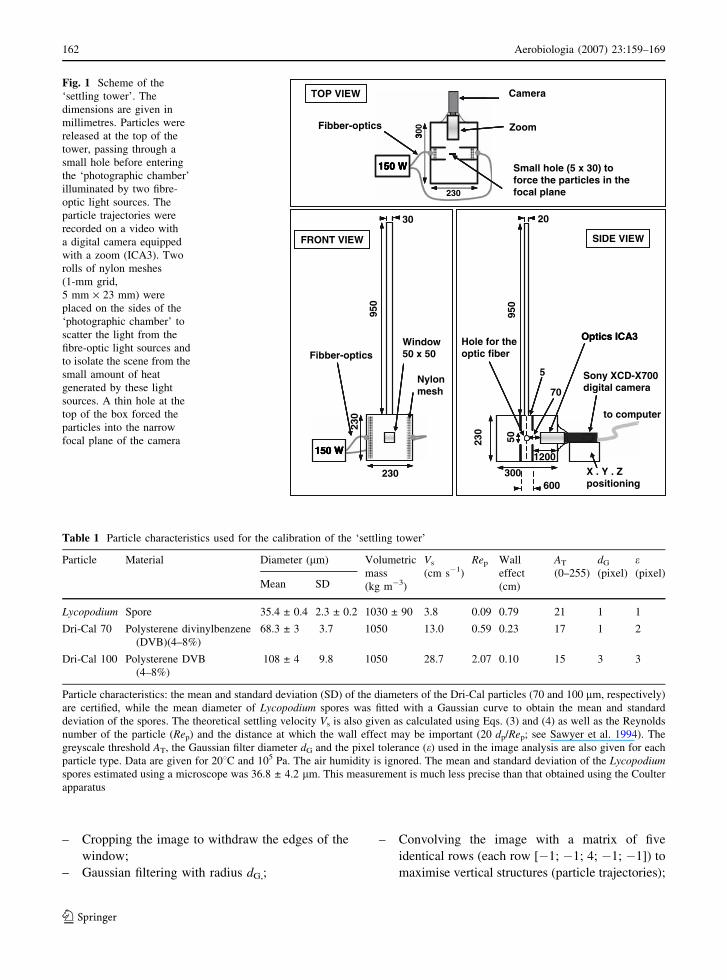
2.1 The ‘settling tower’ apparatus

The scheme and dimensions of the ‘settling tower’

apparatus are given in Fig. 1. In this approach, the

particles are released from a brush placed at a few

millimeters over the top of a 1-m-high stainless steel

tube of a rectangular section. The bottom of the tube

is placed on the top of a wood photographic

chamber with dimensions such as to avoid any

significant wall effects (Table 1). Within the cham-

ber, a window allows filming, while two fibre-optic

light sources illuminate the scene from the sides.

The use of fibre-optic light sources (150 W in total)

avoids overheating of the chamber. The camera

(XCD-X700, Sony, Japan) is equipped with a zoom

(ICA30, 12.5–75 mm, macro, 1:1.8). The tempera-

ture is measured with a mercury thermometer inside

the photographic chamber; in our experiments the

temperature never exceeded 308C. The photographic

chamber is enclosed in a larger box that is

completely sealed and isolated with polystyrene

plates (width: 5 cm). The inside of the photographic

chamber is painted with a black body painting to

avoid any unwanted light reflection. The camera is

connected to a computer for image acquisition with

a frequency f = 15 images s�1. The field of view is

typically 5 cm.

A decametre placed on the side of the film was

used to determine the number of pixels per metre (a).

The light saturation of the camera charge-coupled

device (CCD) sensor was set to the maximum, and

the electronic shutter was set to 42.67 ± 0.005 ms

integration time (s). By doing so, the particles falling

during the time s left a ‘track’ on each image. The

tracks are hereafter called ‘trajectories’. Seven video

files of 1 min were successively recorded as AVI

using SONYCAP software (Sony, Japan), while the

brush was gently tapped.

2.2 Image analysis and data processing

The recorded video files were split into 100-Mo

pieces and analysed with IMAGE J (http://rsb.info.

nih.gov/ij/) with the following sequence of analysis:

– Converting the image to 8 bits with greyscale

from levels 0 to 255;

Aerobiologia (2007) 23:159–169 161

123

– Cropping the image to withdraw the edges of the

window;

– Gaussian filtering with radius dG,;

– Convolving the image with a matrix of five

identical rows (each row [�1; �1; 4; �1; �1]) to

maximise vertical structures (particle trajectories);

X . Y . Z positioning

05

032

059

300600

1200

20

5

SIDE VIEW

Sony XCD-X700digital camera

to computer

70

Hole for the optic fiber

Optics ICA3Optics ICA3

032

059

230

30

Fibber-optics

FRONT VIEW

150 W

Window50 x 50

Nylon mesh

150 W

Fibber-optics

TOP VIEW

Small hole (5 x 30) to force the particles in the focal plane

Camera

Zoom

150 W150 W

003

230

150 W

3

150 W150 W150 W

Fig. 1 Scheme of the

‘settling tower’. The

dimensions are given in

millimetres. Particles were

released at the top of the

tower, passing through a

small hole before entering

the ‘photographic chamber’

illuminated by two fibre-

optic light sources. The

particle trajectories were

recorded on a video with

a digital camera equipped

with a zoom (ICA3). Two

rolls of nylon meshes

(1-mm grid,

5 mm · 23 mm) were

placed on the sides of the

‘photographic chamber’ to

scatter the light from the

fibre-optic light sources and

to isolate the scene from the

small amount of heat

generated by these light

sources. A thin hole at the

top of the box forced the

particles into the narrow

focal plane of the camera

Table 1 Particle characteristics used for the calibration of the ‘settling tower’

Particle Material Diameter (mm) Volumetric

mass

(kg m�3)

Vs

(cm s�1)

Rep Wall

effect

(cm)

AT

(0–255)

dG

(pixel)

e(pixel)

Mean SD

Lycopodium Spore 35.4 ± 0.4 2.3 ± 0.2 1030 ± 90 3.8 0.09 0.79 21 1 1

Dri-Cal 70 Polysterene divinylbenzene

(DVB)(4–8%)

68.3 ± 3 3.7 1050 13.0 0.59 0.23 17 1 2

Dri-Cal 100 Polysterene DVB

(4–8%)

108 ± 4 9.8 1050 28.7 2.07 0.10 15 3 3

Particle characteristics: the mean and standard deviation (SD) of the diameters of the Dri-Cal particles (70 and 100 mm, respectively)

are certified, while the mean diameter of Lycopodium spores was fitted with a Gaussian curve to obtain the mean and standard

deviation of the spores. The theoretical settling velocity Vs is also given as calculated using Eqs. (3) and (4) as well as the Reynolds

number of the particle (Rep) and the distance at which the wall effect may be important (20 dp/Rep; see Sawyer et al. 1994). The

greyscale threshold AT, the Gaussian filter diameter dG and the pixel tolerance (e) used in the image analysis are also given for each

particle type. Data are given for 208C and 105 Pa. The air humidity is ignored. The mean and standard deviation of the Lycopodiumspores estimated using a microscope was 36.8 ± 4.2 mm. This measurement is much less precise than that obtained using the Coulter

apparatus

162 Aerobiologia (2007) 23:159–169

123

– Gaussian filtering with radius dG,;

– Converting the 8-bit image to a binary image

using a greyscale threshold level AT (over 255

levels);

– Identifying each object in the image with the

macro ANALYZE PARTICLES, based on the use of the

WAND method.

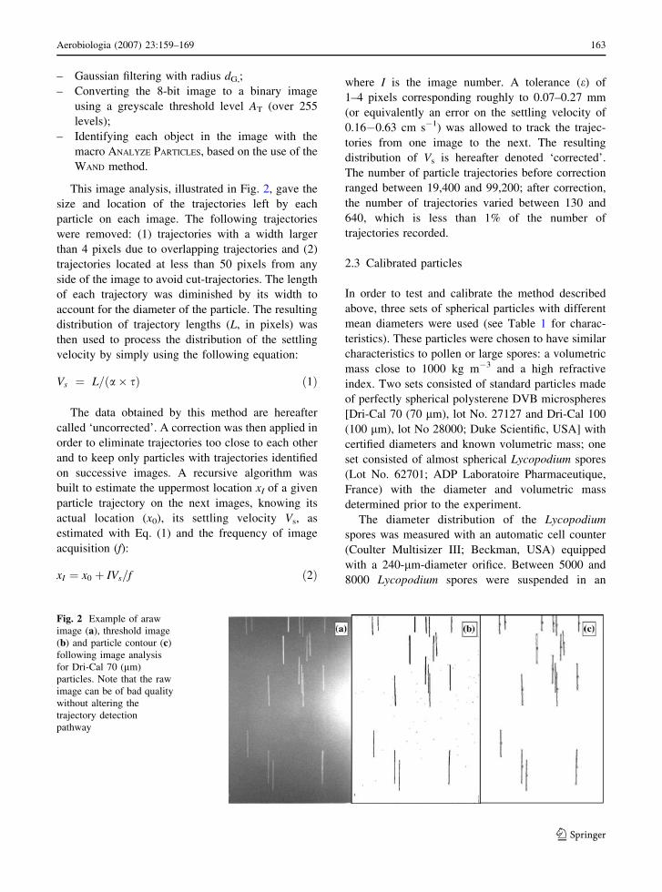
This image analysis, illustrated in Fig. 2, gave the

size and location of the trajectories left by each

particle on each image. The following trajectories

were removed: (1) trajectories with a width larger

than 4 pixels due to overlapping trajectories and (2)

trajectories located at less than 50 pixels from any

side of the image to avoid cut-trajectories. The length

of each trajectory was diminished by its width to

account for the diameter of the particle. The resulting

distribution of trajectory lengths (L, in pixels) was

then used to process the distribution of the settling

velocity by simply using the following equation:

Vs ¼ L=ða� sÞ ð1Þ

The data obtained by this method are hereafter

called ‘uncorrected’. A correction was then applied in

order to eliminate trajectories too close to each other

and to keep only particles with trajectories identified

on successive images. A recursive algorithm was

built to estimate the uppermost location xI of a given

particle trajectory on the next images, knowing its

actual location (x0), its settling velocity Vs, as

estimated with Eq. (1) and the frequency of image

acquisition (f):

xI ¼ x0 þ IVs=f ð2Þ

where I is the image number. A tolerance (e) of

1–4 pixels corresponding roughly to 0.07–0.27 mm

(or equivalently an error on the settling velocity of

0.16�0.63 cm s�1) was allowed to track the trajec-

tories from one image to the next. The resulting

distribution of Vs is hereafter denoted ‘corrected’.

The number of particle trajectories before correction

ranged between 19,400 and 99,200; after correction,

the number of trajectories varied between 130 and

640, which is less than 1% of the number of

trajectories recorded.

2.3 Calibrated particles

In order to test and calibrate the method described

above, three sets of spherical particles with different

mean diameters were used (see Table 1 for charac-

teristics). These particles were chosen to have similar

characteristics to pollen or large spores: a volumetric

mass close to 1000 kg m�3 and a high refractive

index. Two sets consisted of standard particles made

of perfectly spherical polysterene DVB microspheres

[Dri-Cal 70 (70 mm), lot No. 27127 and Dri-Cal 100

(100 mm), lot No 28000; Duke Scientific, USA] with

certified diameters and known volumetric mass; one

set consisted of almost spherical Lycopodium spores

(Lot No. 62701; ADP Laboratoire Pharmaceutique,

France) with the diameter and volumetric mass

determined prior to the experiment.

The diameter distribution of the Lycopodium

spores was measured with an automatic cell counter

(Coulter Multisizer III; Beckman, USA) equipped

with a 240-mm-diameter orifice. Between 5000 and

8000 Lycopodium spores were suspended in an

Fig. 2 Example of araw

image (a), threshold image

(b) and particle contour (c)

following image analysis

for Dri-Cal 70 (mm)

particles. Note that the raw

image can be of bad quality

without altering the

trajectory detection

pathway

Aerobiologia (2007) 23:159–169 163

123

electrolyte solution (Coulter Isoton, Beckman) and

counted within the next minute. The operation was

repeated 20 times. The diameter distribution was

then fit with a Gaussian curve to obtain the mean

and standard deviation (Table 1). We calculated the

mean diameter of the Lycopodium spores to be

35.4 mm, which is similar to the 35.6 mm reported

by Rambert et al. (1998) using both a phase-doppler

method and a laser-diffraction spectrometer method.

However, it is larger than the 32.8 mm reported by

Ferrandino and Aylor (1984). Visual control of the

spores with a microscope showed that the spores

were tetrahedral, as expected, with a smaller

dimension of 34.4 mm and a larger dimension of

39.3 mm, giving a ratio of larger to smaller

dimension q = 1.15; the corresponding average

and standard deviation of the diameter is 36.8 and

4.2 mm, respectively.

The Lycopodium spores were suspended in the

electrolyte solution for less than 1 min in order to

avoid changes in their diameter. Preliminary exper-

iments had proven that 1 min is sufficiently short to

avoid the spores absorbing electrolyte solution and

consequently increasing their diameter; in contrast,

the diameter of the spores could increase from 35 to

38 mm over a 30-min period in the electrolyte

solution. Consequently, the Lycopodium spores were

kept in a dry environment (laboratory).

The volumetric mass of the three sets of

spherical particles was measured by weighing a

10- to 20-mg sample of particles on a precision

balance (precision: 0.1 mg). The sample was then

put into a known volume of the electrolyte solution.

The volume of particles contained in 1 ml of the

solution was determined ten times within a very

short time period (less than 1 min) using the

automatic counter. This procedure was repeated five

times. The uncertainty of the method was estimated

from the uncertainty of the balance and the standard

deviation of the counted volume of particles over

50 repetitions.

2.4 Theoretical settling velocity

The theoretical settling velocity of calibrated parti-

cles was calculated using the parameterisation given

by Aylor (2002) and taken from Fuchs (1964), over a

wide range of Reynolds number Rep (from

0.001 to 200):

V2s ¼

4gdpqp

3CDqa

ð3Þ

CD ¼24

Rep

1þ 0:158Re2=3p

� �ð4Þ

where dp and qp are particle diameter and volumetric

mass, respectively and qa is the air volumetric mass.

The particle inertial time scale sp is defined as sp = Vs

g�1. The characteristic distance required for the

particle velocity to reach its terminal velocity was

estimated in a simplified way as Z = sp Vs = Vs2 g�1.

For all particles, it was smaller than 1 cm. The height

of the ‘settling tower’ was, however, high enough to

minimise the influence of the external turbulence

inside the photographic chamber.

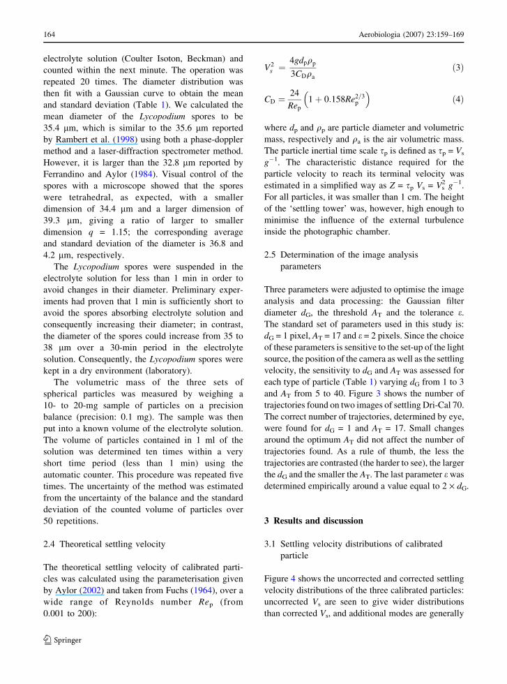
2.5 Determination of the image analysis

parameters

Three parameters were adjusted to optimise the image

analysis and data processing: the Gaussian filter

diameter dG, the threshold AT and the tolerance e.The standard set of parameters used in this study is:

dG = 1 pixel, AT = 17 and e = 2 pixels. Since the choice

of these parameters is sensitive to the set-up of the light

source, the position of the camera as well as the settling

velocity, the sensitivity to dG and AT was assessed for

each type of particle (Table 1) varying dG from 1 to 3

and AT from 5 to 40. Figure 3 shows the number of

trajectories found on two images of settling Dri-Cal 70.

The correct number of trajectories, determined by eye,

were found for dG = 1 and AT = 17. Small changes

around the optimum AT did not affect the number of

trajectories found. As a rule of thumb, the less the

trajectories are contrasted (the harder to see), the larger

the dG and the smaller the AT. The last parameter e was

determined empirically around a value equal to 2 · dG.

3 Results and discussion

3.1 Settling velocity distributions of calibrated

particle

Figure 4 shows the uncorrected and corrected settling

velocity distributions of the three calibrated particles:

uncorrected Vs are seen to give wider distributions

than corrected Vs, and additional modes are generally

164 Aerobiologia (2007) 23:159–169

123

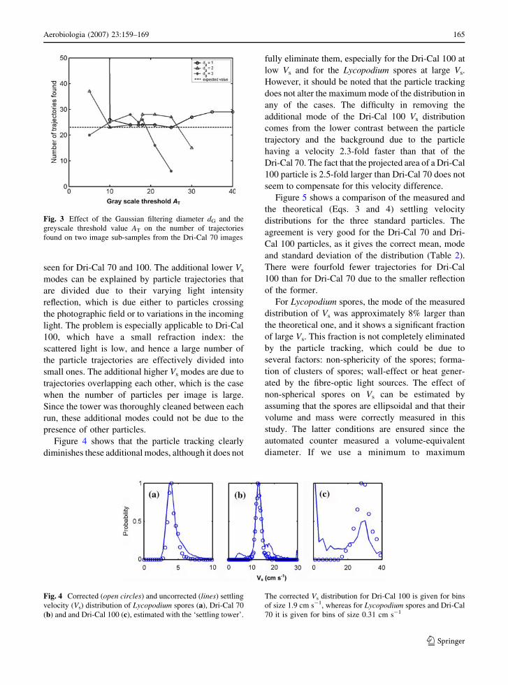
seen for Dri-Cal 70 and 100. The additional lower Vs

modes can be explained by particle trajectories that

are divided due to their varying light intensity

reflection, which is due either to particles crossing

the photographic field or to variations in the incoming

light. The problem is especially applicable to Dri-Cal

100, which have a small refraction index: the

scattered light is low, and hence a large number of

the particle trajectories are effectively divided into

small ones. The additional higher Vs modes are due to

trajectories overlapping each other, which is the case

when the number of particles per image is large.

Since the tower was thoroughly cleaned between each

run, these additional modes could not be due to the

presence of other particles.

Figure 4 shows that the particle tracking clearly

diminishes these additional modes, although it does not

fully eliminate them, especially for the Dri-Cal 100 at

low Vs and for the Lycopodium spores at large Vs.

However, it should be noted that the particle tracking

does not alter the maximum mode of the distribution in

any of the cases. The difficulty in removing the

additional mode of the Dri-Cal 100 Vs distribution

comes from the lower contrast between the particle

trajectory and the background due to the particle

having a velocity 2.3-fold faster than that of the

Dri-Cal 70. The fact that the projected area of a Dri-Cal

100 particle is 2.5-fold larger than Dri-Cal 70 does not

seem to compensate for this velocity difference.

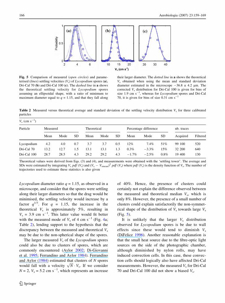
Figure 5 shows a comparison of the measured and

the theoretical (Eqs. 3 and 4) settling velocity

distributions for the three standard particles. The

agreement is very good for the Dri-Cal 70 and Dri-

Cal 100 particles, as it gives the correct mean, mode

and standard deviation of the distribution (Table 2).

There were fourfold fewer trajectories for Dri-Cal

100 than for Dri-Cal 70 due to the smaller reflection

of the former.

For Lycopodium spores, the mode of the measured

distribution of Vs was approximately 8% larger than

the theoretical one, and it shows a significant fraction

of large Vs. This fraction is not completely eliminated

by the particle tracking, which could be due to

several factors: non-sphericity of the spores; forma-

tion of clusters of spores; wall-effect or heat gener-

ated by the fibre-optic light sources. The effect of

non-spherical spores on Vs can be estimated by

assuming that the spores are ellipsoidal and that their

volume and mass were correctly measured in this

study. The latter conditions are ensured since the

automated counter measured a volume-equivalent

diameter. If we use a minimum to maximum

Fig. 3 Effect of the Gaussian filtering diameter dG and the

greyscale threshold value AT on the number of trajectories

found on two image sub-samples from the Dri-Cal 70 images

Fig. 4 Corrected (open circles) and uncorrected (lines) settling

velocity (Vs) distribution of Lycopodium spores (a), Dri-Cal 70

(b) and and Dri-Cal 100 (c), estimated with the ‘settling tower’.

The corrected Vs distribution for Dri-Cal 100 is given for bins

of size 1.9 cm s�1, whereas for Lycopodium spores and Dri-Cal

70 it is given for bins of size 0.31 cm s�1

Aerobiologia (2007) 23:159–169 165

123

Lycopodium diameter ratio q = 1.15, as observed in a

microscope, and consider that the spores were settling

along their larger diameters so that the drag would be

minimised, the settling velocity would increase by a

factor q1/3. For q = 1.15, the increase in the

theoretical Vs is approximately 5%, resulting in

Vs = 3.9 cm s�1. This latter value would fit better

with the measured mode of Vs of 4 cm s�1 (Fig. 4a;

Table 2), lending support to the hypothesis that the

discrepancy between the measured and theoretical Vs

may be due to the non-spherical shape of the spores.

The larger measured Vs of the Lycopodium spores

could also be due to clusters of spores, which are

commonly encountered (Aylor 2002; Di-Giovanni

et al. 1995; Ferrandino and Aylor 1984). Ferrandino

and Aylor (1984) estimated that clusters of N spores

would fall with a velocityffiffiffiffiNp� Vs. If we consider

N = 2, Vs = 5.2 cm s�1, which represents an increase

of 40%. Hence, the presence of clusters could

certainly not explain the difference observed between

the measured and theoretical median Vs, which is

only 8%. However, the presence of a small number of

clusters could explain satisfactorily the non-symmet-

rical shape of the distribution of Vs towards large Vs

(Fig. 5).

It is unlikely that the larger Vs distribution

observed for Lycopodium spores is be due to wall

effects since these would tend to diminish Vs

(DiFelice 1996). Another reasonable explanation is

that the small heat source due to the fibre-optic light

sources on the side of the photographic chamber,

although diminished by nylon rolls, may have

induced convection cells. In this case, these convec-

tion cells should logically also have affected Dri-Cal

measurements. However, the measured Vs for Dri-Cal

70 and Dri-Cal 100 did not show a biased Vs.

Fig. 5 Comparison of measured (open circles) and parame-

terised (lines) settling velocities (Vs) of Lycopodium spores (a),

Dri-Cal 70 (b) and Dri-Cal 100 (c). The dashed line in a shows

the theoretical settling velocity for Lycopodium spores

assuming an ellipsoidal shape, with a ratio of minimum to

maximum diameter equal to q = 1.15, and that they fall along

their larger diameter. The dotted line in a shows the theoretical

Vs obtained when using the mean and standard deviation

diameter estimated in the microscope �36.8 ± 4.2 mm. The

corrected Vs distribution for Dri-Cal 100 is given for bins of

size 1.9 cm s�1, whereas for Lycopodium spores and Dri-Cal

70, it is given for bins of size 0.31 cm s�1

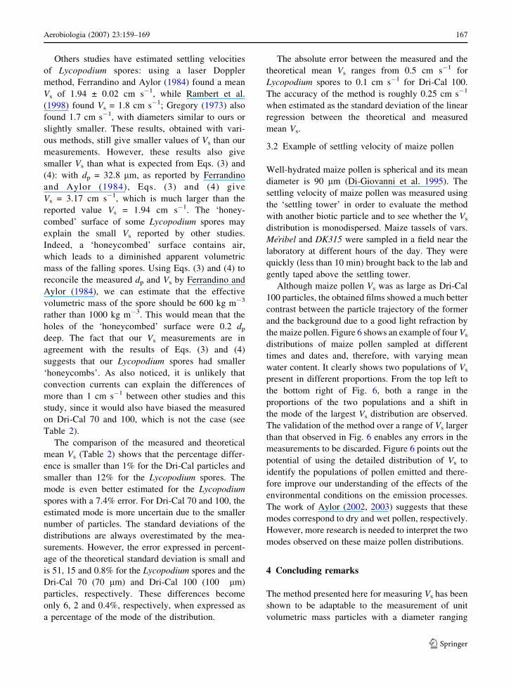
Table 2 Measured versus theoretical average and standard deviation of the settling velocity distribution Vs for three calibrated

particles

Vs (cm s�1)

Particle Measured Theoretical Percentage difference nb. traces

Mean Mode SD Mean Mode SD Mean Mode SD Acquired Filtered

Lycopodium 4.2 4.0 0.7 3.7 3.7 0.5 12% 7.4% 51% 99 100 520

Dri-Cal 70 13.2 12.7 1.5 13.1 13.1 1.3 0.3% �3.3% 15% 32 200 640

Dri-Cal 100 28.7 28.5 4.3 29.2 29.2 4.3 �1.7% �2.5% 0.8% 19 400 130

Theoretical values were derived from Eqs. (3) and (4), and measurements were obtained with the ‘settling tower’. The average and

SDs were estimated by integrating Vs pdf (Vs) and (Vs � Vsmean)2 pdf (Vs) where pdf (Vs) is the density function of Vs. The number of

trajectories used to estimate these statistics is also given

166 Aerobiologia (2007) 23:159–169

123

Others studies have estimated settling velocities

of Lycopodium spores: using a laser Doppler

method, Ferrandino and Aylor (1984) found a mean

Vs of 1.94 ± 0.02 cm s�1, while Rambert et al.

(1998) found Vs = 1.8 cm s�1; Gregory (1973) also

found 1.7 cm s�1, with diameters similar to ours or

slightly smaller. These results, obtained with vari-

ous methods, still give smaller values of Vs than our

measurements. However, these results also give

smaller Vs than what is expected from Eqs. (3) and

(4): with dp = 32.8 mm, as reported by Ferrandino

and Aylor (1984), Eqs. (3) and (4) give

Vs = 3.17 cm s�1, which is much larger than the

reported value Vs = 1.94 cm s�1. The ‘honey-

combed’ surface of some Lycopodium spores may

explain the small Vs reported by other studies.

Indeed, a ‘honeycombed’ surface contains air,

which leads to a diminished apparent volumetric

mass of the falling spores. Using Eqs. (3) and (4) to

reconcile the measured dp and Vs by Ferrandino and

Aylor (1984), we can estimate that the effective

volumetric mass of the spore should be 600 kg m�3

rather than 1000 kg m�3. This would mean that the

holes of the ‘honeycombed’ surface were 0.2 dp

deep. The fact that our Vs measurements are in

agreement with the results of Eqs. (3) and (4)

suggests that our Lycopodium spores had smaller

‘honeycombs’. As also noticed, it is unlikely that

convection currents can explain the differences of

more than 1 cm s�1 between other studies and this

study, since it would also have biased the measured

on Dri-Cal 70 and 100, which is not the case (see

Table 2).

The comparison of the measured and theoretical

mean Vs (Table 2) shows that the percentage differ-

ence is smaller than 1% for the Dri-Cal particles and

smaller than 12% for the Lycopodium spores. The

mode is even better estimated for the Lycopodium

spores with a 7.4% error. For Dri-Cal 70 and 100, the

estimated mode is more uncertain due to the smaller

number of particles. The standard deviations of the

distributions are always overestimated by the mea-

surements. However, the error expressed in percent-

age of the theoretical standard deviation is small and

is 51, 15 and 0.8% for the Lycopodium spores and the

Dri-Cal 70 (70 mm) and Dri-Cal 100 (100 mm)

particles, respectively. These differences become

only 6, 2 and 0.4%, respectively, when expressed as

a percentage of the mode of the distribution.

The absolute error between the measured and the

theoretical mean Vs ranges from 0.5 cm s�1 for

Lycopodium spores to 0.1 cm s�1 for Dri-Cal 100.

The accuracy of the method is roughly 0.25 cm s�1

when estimated as the standard deviation of the linear

regression between the theoretical and measured

mean Vs.

3.2 Example of settling velocity of maize pollen

Well-hydrated maize pollen is spherical and its mean

diameter is 90 mm (Di-Giovanni et al. 1995). The

settling velocity of maize pollen was measured using

the ‘settling tower’ in order to evaluate the method

with another biotic particle and to see whether the Vs

distribution is monodispersed. Maize tassels of vars.

Meribel and DK315 were sampled in a field near the

laboratory at different hours of the day. They were

quickly (less than 10 min) brought back to the lab and

gently taped above the settling tower.

Although maize pollen Vs was as large as Dri-Cal

100 particles, the obtained films showed a much better

contrast between the particle trajectory of the former

and the background due to a good light refraction by

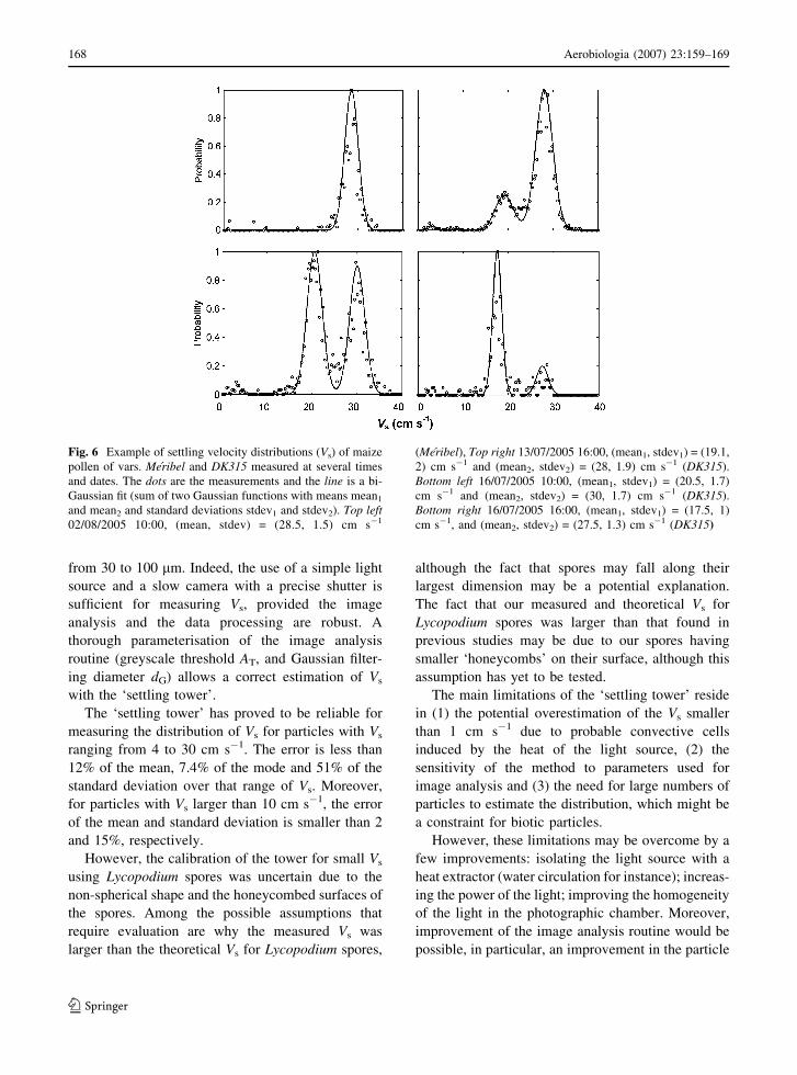
the maize pollen. Figure 6 shows an example of four Vs

distributions of maize pollen sampled at different

times and dates and, therefore, with varying mean

water content. It clearly shows two populations of Vs

present in different proportions. From the top left to

the bottom right of Fig. 6, both a range in the

proportions of the two populations and a shift in

the mode of the largest Vs distribution are observed.

The validation of the method over a range of Vs larger

than that observed in Fig. 6 enables any errors in the

measurements to be discarded. Figure 6 points out the

potential of using the detailed distribution of Vs to

identify the populations of pollen emitted and there-

fore improve our understanding of the effects of the

environmental conditions on the emission processes.

The work of Aylor (2002, 2003) suggests that these

modes correspond to dry and wet pollen, respectively.

However, more research is needed to interpret the two

modes observed on these maize pollen distributions.

4 Concluding remarks

The method presented here for measuring Vs has been

shown to be adaptable to the measurement of unit

volumetric mass particles with a diameter ranging

Aerobiologia (2007) 23:159–169 167

123

from 30 to 100 mm. Indeed, the use of a simple light

source and a slow camera with a precise shutter is

sufficient for measuring Vs, provided the image

analysis and the data processing are robust. A

thorough parameterisation of the image analysis

routine (greyscale threshold AT, and Gaussian filter-

ing diameter dG) allows a correct estimation of Vs

with the ‘settling tower’.

The ‘settling tower’ has proved to be reliable for

measuring the distribution of Vs for particles with Vs

ranging from 4 to 30 cm s�1. The error is less than

12% of the mean, 7.4% of the mode and 51% of the

standard deviation over that range of Vs. Moreover,

for particles with Vs larger than 10 cm s�1, the error

of the mean and standard deviation is smaller than 2

and 15%, respectively.

However, the calibration of the tower for small Vs

using Lycopodium spores was uncertain due to the

non-spherical shape and the honeycombed surfaces of

the spores. Among the possible assumptions that

require evaluation are why the measured Vs was

larger than the theoretical Vs for Lycopodium spores,

although the fact that spores may fall along their

largest dimension may be a potential explanation.

The fact that our measured and theoretical Vs for

Lycopodium spores was larger than that found in

previous studies may be due to our spores having

smaller ‘honeycombs’ on their surface, although this

assumption has yet to be tested.

The main limitations of the ‘settling tower’ reside

in (1) the potential overestimation of the Vs smaller

than 1 cm s�1 due to probable convective cells

induced by the heat of the light source, (2) the

sensitivity of the method to parameters used for

image analysis and (3) the need for large numbers of

particles to estimate the distribution, which might be

a constraint for biotic particles.

However, these limitations may be overcome by a

few improvements: isolating the light source with a

heat extractor (water circulation for instance); increas-

ing the power of the light; improving the homogeneity

of the light in the photographic chamber. Moreover,

improvement of the image analysis routine would be

possible, in particular, an improvement in the particle

Fig. 6 Example of settling velocity distributions (Vs) of maize

pollen of vars. Meribel and DK315 measured at several times

and dates. The dots are the measurements and the line is a bi-

Gaussian fit (sum of two Gaussian functions with means mean1

and mean2 and standard deviations stdev1 and stdev2). Top left02/08/2005 10:00, (mean, stdev) = (28.5, 1.5) cm s�1

(Meribel), Top right 13/07/2005 16:00, (mean1, stdev1) = (19.1,

2) cm s�1 and (mean2, stdev2) = (28, 1.9) cm s�1 (DK315).

Bottom left 16/07/2005 10:00, (mean1, stdev1) = (20.5, 1.7)

cm s�1 and (mean2, stdev2) = (30, 1.7) cm s�1 (DK315).

Bottom right 16/07/2005 16:00, (mean1, stdev1) = (17.5, 1)

cm s�1, and (mean2, stdev2) = (27.5, 1.3) cm s�1 (DK315)

168 Aerobiologia (2007) 23:159–169

123

tracking between successive images would increase

the robustness of the method and allow the lower

trajectories to be rejected. We also recommend that a

systematic sensitivity study should be performed to

define the optimum parameters of the image analysis

for each new setting of the tower.

As suggested by preliminary measurements, the

‘settling tower’ could be of great practical interest for

measuring the distribution of Vs of maize pollen.

Moreover, given that a large number of pollen and

spores have a diameter between 30 and than 100 mm,

this method could be applied to most other types of

pollen or spores. For these particles, Vs measurements

would allow their potential for dispersal in the

atmosphere to be estimated and provide input for

dispersal models, such as those of Aylor et al. (2003)

and Jarosz et al. (2004). Moreover, Vs may be used as

a manner to characterize the presence of several

populations of pollens within a sample, such as the

number of dehydrated pollen or clusters of pollen.

References

Adrian, R. J. (1991). Particle-imaging techniques for experi-

mental fluid mechanics. Annual Review of FluidMechanics, 23, 261–304.

Aylor, D. E. (2002). Settling speed of corn (Zea mays) pollen.

Journal of Aerosol Science, 33, 1601–1607.

Aylor, D. E. (2003). Rate of dehydration of corn (Zea mays L.)

pollen in the air. Journal of Experimental Botany, 54,

2307–2312.

Aylor, D. E., & Taylor, G. S. (1983). Escape of PeronosporaTabacina spores from a field of diseased Tobacco plants.

Phytopathology, 73, 525–529.

Aylor, D. E., & Irwin, M. E. (1999). Aerial dispersal of pests

and pathogens: implications for integrated pest manage-

ment. Agricultural and Forest Meteorology, 97, 233–234.

Aylor, D. E., Schultes, N. P., & Shields, E. J. (2003). An aero-

biological framework for assessing cross-pollination in

maize. Agricultural and Forest Meteorology, 119, 111–129.

DiFelice, R. (1996). A relationship for the wall effect on the

settling velocity of a sphere at any flow regime. Interna-tional Journal of Multiphase Flow, 22, 527–533.

Di-Giovanni, F., Kevan, P. G., & Nasr, M. E. (1995). The

variability in settling velocities of some pollen and spores.

Grana, 34, 39–44.

Dupont, S., Brunet, Y., & Jarosz, N. (2006). Eulerian modelling

of pollen dispersal over heterogenous vegetation canopies.

Agricultural and Forest Meteorology, 141, 82–104.

Ferrandino, F. J., & Aylor, D. E. (1984). Settling speed of

clusters of spores. Phytopatholgy, 74, 969–972.

Fields, T. B. (2002). Aerodynamic time-of-flight particle size

measurement. Journal of Dispersion Science and Tech-nology, 23, 729–735.

Fuchs, N. A. (1964). The mechanics of aerosols. New York:

Macmillan.

Gregory, P. H. (1973). Microbiology of the atmosphere. New

York: John Wiley & Sons.

Haskell, G., & Dow, P. (1951). Studies with sweet corn V.

Seed-settings with distances from pollen source. EmpireJournal of Experimental Agriculture, 19, 45–50.

Jarosz, N., Loubet, B., Durand, B., McCartney, H. A., Fouei-

llassar, X., & Huber, L. (2003). Field measurements of

airborne concentration and deposition of maize pollen.

Agricultural and Forest Meteorology, 119, 37–51.

Jarosz, N., Loubet, B., & Huber, L. (2004). Modelling airborne

concentration and deposition rate of maize pollen. Atmo-spheric Environment, 38, 5555–5566.

Jarosz, N., Loubet, B., Durand, B., Foueillassar, X., & Huber,

L. (2005). Variations in maize pollen emission and

deposition in relation to microclimate. EnvironmentalScience and Technology, 39, 4377–4384.

Klein, E. K., Lavigne, C., Foueillassar, X., Gouyon, P. H., &

Laredo, C. (2003). Corn pollen dispersal: Quasi-mecha-

nistic models and field experiments. Ecological Mono-graphs, 73, 131–150.

Lavigne, C., Godelle, B., Reboud, X., & Gouyon, P. H. (1996).

A method to determine the mean pollen dispersal of

individual plants growing within a large pollen source.

Theoretical and Applied Genetics, 93, 1319–1326.

Lavigne, C., Klein, E. K., Vallee, P., Pierre, J., Godelle, B., &

Renard, M. (1998). A pollen-dispersal experiment with

transgenic oilseed rape. Estimation of the average pollen

dispersal of an individual plant within a field. Theoreticaland Applied Genetics, 96, 886–896.

Lavigne, C., Klein, E. K., & Couvet, D. (2002). Using seed

purity data to estimate an average pollen mediated gene

flow from crops to wild relatives. Theoretical and AppliedGenetics, 104, 139–145.

Luna, V. S., Figueroa M. J., Baltazar M. B., Gomez L. R.,

Townsend R., & Schoper, J. B. (2001). Maize pollen

longevity and distance isolation requirements for effective

pollen control. Crop Science, 41, 1551–1557.

Malcolm, L. P., & Raupach, M. R. (1991). Measurements in an

air settling tube of the terminal velocity distribution of soil

material. Journal of Geophysical Research, 96, 15275–

15286.

McCartney, H. A. (1994). Dispersal of spores and pollen from

crops. Grana, 33, 76–80.

Rambert, A., Huber, L., & Gougat., P. (1998). Laboratory

study of fungal spore movement using Laser Doppler

Velocimetry. Agricultural and Forest Meteorology, 92,

43–53.

Renoux, A., & Boulaud, D. (1998). Les aerosols. Physique etMetrologie. Paris: Lavoisier.

Sawyer, A. J., Griggs, M. H., & Wayne, R. (1994). Dimen-

sions, density, and settling velocity of entomophthoralean

Conidia : implications for aerial dissemination of spores.

Journal of Invertebrate Pathology, 63, 43–55.

Seinfeld, J. H., & Pandis, S. N. (1998). Atmospheric chemistryand physics. From air pollution to climate change. New

York: Wiley-Interscience.

Aerobiologia (2007) 23:159–169 169

123