Ž . Parallel Computing 24 1998 221–245 A method for exploiting communicationrcomputation overlap in hypercubes 1 Luis Dıaz de Cerio ) , Miguel Valero-Garcıa 2 , Antonio Gonzalez 3 ´ ´ ´ Departament d’Arquitectura de Computadors, UniÕersitat Politecnica de Catalunya, c r Jordi Girona 1– 3, ` Campus Nord — Edifici D6, E-08034 Barcelona, Spain Received 19 December 1996; revised 29 July 1997 Abstract This paper presents a method to derive efficient algorithms for hypercubes. The method . exploits two features of the underlying hardware: a the parallelism provided by the multiple . communication links of each node and b the possibility of overlapping computations and communications which is a feature of machines supporting an asynchronous communication protocol. The method can be applied to a generic class of hypercube algorithms whose distinguish- ing features are quite frequent in common algorithms for hypercubes. Many examples of this class of algorithms are found in the literature for different problems. The paper shows the efficiency of the method for two case studies. The results show that the reduction in communication overhead is very significant in many cases. They also show that the algorithms produced by our method are always very close to the optimum in terms of execution time. q 1998 Elsevier Science B.V. All rights reserved. Keywords: Hypercube; Communication pipelining; Communicationrcomputation overlap; Performance mod- eling; FFT; Vector Add ) Corresponding author. E-mail: [email protected] 1 Ž . Expanded version of a talk presented at Euro-Par’96 Lyon, France, August 1996 . 2 E-mail: [email protected] 3 E-mail: [email protected] 0167-8191r98r$19.00 q 1998 Elsevier Science B.V. All rights reserved. Ž . PII S0167-8191 98 00005-2

Welcome message from author
This document is posted to help you gain knowledge. Please leave a comment to let me know what you think about it! Share it to your friends and learn new things together.
Transcript
Ž .Parallel Computing 24 1998 221–245
A method for exploitingcommunicationrcomputation overlap in
hypercubes 1
Luis Dıaz de Cerio ), Miguel Valero-Garcıa 2, Antonio Gonzalez 3´ ´ ´Departament d’Arquitectura de Computadors, UniÕersitat Politecnica de Catalunya, cr Jordi Girona 1– 3,`
Campus Nord — Edifici D6, E-08034 Barcelona, Spain
Received 19 December 1996; revised 29 July 1997
Abstract
This paper presents a method to derive efficient algorithms for hypercubes. The method.exploits two features of the underlying hardware: a the parallelism provided by the multiple
.communication links of each node and b the possibility of overlapping computations andcommunications which is a feature of machines supporting an asynchronous communicationprotocol. The method can be applied to a generic class of hypercube algorithms whose distinguish-ing features are quite frequent in common algorithms for hypercubes. Many examples of this classof algorithms are found in the literature for different problems. The paper shows the efficiency ofthe method for two case studies. The results show that the reduction in communication overhead isvery significant in many cases. They also show that the algorithms produced by our method arealways very close to the optimum in terms of execution time. q 1998 Elsevier Science B.V. Allrights reserved.
Keywords: Hypercube; Communication pipelining; Communicationrcomputation overlap; Performance mod-eling; FFT; Vector Add
) Corresponding author. E-mail: [email protected] Ž .Expanded version of a talk presented at Euro-Par’96 Lyon, France, August 1996 .2 E-mail: [email protected] E-mail: [email protected]
0167-8191r98r$19.00 q 1998 Elsevier Science B.V. All rights reserved.Ž .PII S0167-8191 98 00005-2
( )L. Dıaz de Cerio et al.rParallel Computing 24 1998 221–245´222
1. Introduction
The hypercube has been extensively used as interconnection topology for multicom-w x w xputers 1 and as a communication topology for parallel algorithms 2,3 .
Properties such as regularity, low diameter, low average distance and high communi-cation bandwidth make the hypercube very attractive for connecting a smallrmedium
Ž .number of nodes up to 1024 . On the other hand, since the number of links per nodeincreases with the number of nodes, hypercubes are not so scalable as other topologieslike meshes and tori, which may be more appropriate for very large systems.
Besides, the recursive nature of hypercubes facilitates the development of manyparallel algorithms in terms of a set of processes using a hypercube communicationtopology.
Communication overhead is a crucial issue when considering the performance of amulticomputer. In some cases, communication overhead is the most significant factor inthe execution time. To help in reducing communication overhead, the nodes of amulticomputer can be designed with the following capabilities:Ž . Ža Sending several messages in parallel through different links communication
.parallelism , androrŽ .b Overlapping communication through one or several links with computation in the
Ž .node communicationrcomputation overlapping .Ž . Ž .Designing parallel algorithms which are able to exploit features a andror b is not
w xan easy task. Many of those natural and elegant hypercube algorithms found in 2,3cannot exploit these features efficiently. In any case, some papers can be found in theliterature which propose hypercube algorithms for particular problems which are effi-
w xcient for particular machine configurations. Examples are 4–9 , just to mention a few.In this paper we propose a method to derive hypercube algorithms which are able to
Ž . Ž .exploit features a and b . The method takes as an starting point a hypercube algorithmto solve the problem and transforms it in a systematic way, using a technique that wecall communication pipelining, which basically splits each message into small pieceswhich are sent in a pipelined fashion. The starting algorithm must belong to a class ofhypercube algorithms which we call Compute and Communicate hypercube algorithmsŽ .CC-cube algorithms with some particular features which enable the application ofcommunication pipelining. Many numerical and symbolic computation problems can be
w x w xsolved using a CC-cube algorithm. FFT 7 , Hartley transform 10 , All-to-All personal-w xized communications 11 and Jacobi methods for singular value decomposition and
w xeigenvalue computation 12 are just some examples.There are two reasons which makes the proposed method very attractive. First, it is a
general method in the sense that it can be applied to any CC-cube algorithm. Asmentioned before, previous proposals are particular schemes for particular applications.Second, the method allows tuning the level of communication parallelism and communi-cationrcomputation overlapping in order to minimize the communication overhead. Thisfeature allows us to obtain efficient algorithms, very close to the optimum, even inmachine configurations with extremely slow communication hardware.
In this paper, performance figures are given for two concrete application examples:FFT and Vector Add. Hypercube algorithms for FFT have been extensively studied in
( )L. Dıaz de Cerio et al.rParallel Computing 24 1998 221–245´ 223
w xthe literature. Among others, 5,7 are two concrete examples of algorithms which try tow x w xexploit communication parallelism 7 and communicationrcomputation overlapping 5 .
In both cases the degree of communication parallelism and overlapping is fixed and,therefore, the results are only efficient for some machine configurations. The results of
w xthe proposed method for the case of FFT will be compared to those presented in 5,7 .The Vector Add is an example of an application in which the communication
Ž .requirements of the problem are very high much higher than in the case of FFT . Evenin this situation the proposed method gives efficient results.
The communication pipelining technique, which is the basis of the proposed method,w xhas been used in a previous paper 13 , in which only communication parallelism is
considered. The main contribution of the present paper is the extension of the method inorder to include the overlapping of communications and computations. A preliminary
w xand concise version of this work was published in 14 .The rest of the paper is organized as follows. Section 2 describes the assumed
architecture. Section 3 defines the concept of CC-cube algorithm. Section 4 reviews theconcept of communication pipelining. Section 5 establish the overlapping method that isbased on the previously described concept of communication pipelining. Section 6defines the analytical models for the execution time of the algorithms. Section 7describes a strategy to obtain the degree of pipelining that minimizes the execution time.Section 8 shows some performance figures of the method. Finally, the main conclusionsof this work are drawn in Section 9.
2. Target architecture
This study assumes a distributed memory multicomputer consisting of 2 d processorsconnected by bidirectional point-to-point links in a d-dimensional hypercube topology.Every node can send messages to any of its d neighbors following an asynchronousprotocol. This means that, after initiating a communication operation through one orseveral of its links, a processor can continue performing computations in parallel withthe transmission of the data. The time required for a message of size L to go from anode to one of its neighbors is:
T qLT , 1Ž .sup e
where T is the communication start-up and T is the communication time per sizesup eŽunit. This model is valid for any control flow method store-and-forward, wormhole,
.circuit switching since the communication always take place between neighbor nodes.It is also assumed that every node can send messages in parallel along different links
of the hypercube. However, the start-up times for the different communications cannotŽbe overlapped we assume that T corresponds mostly to time spent by the processor tosup
.initiate each transmission . Therefore, the cost of sending c messages in parallel along cdifferent dimensions of the hypercube and performing afterwards a computation thatrequires A units of time is considered to be:
� 4cT qmax A , L T , 2Ž .sup max e
( )L. Dıaz de Cerio et al.rParallel Computing 24 1998 221–245´224
where L is the size of the longest message to be sent. This is in fact an upper boundmax
that will be exact only in the case that the longest message is the last one to be sent.Note that this expression assumes no contention on the node-internal bus or memory.
This contention depends on the memory organization and may not be null for some realmachines. However, in order to take advantage of the possibility of using several linksin parallel, this contention should be very low or otherwise, the final performance willbe similar to sending the messages sequentially one after the other. In this scenario, theadditional cost required to implement parallel communications in each node will hardlybe rewarding.
3. CC-cube algorithms
In this section, the class of parallel algorithms to which the proposed method can beapplied is defined. The algorithms that fit into this class will be called Compute andCommunicate hypercube algorithms, CC-cube algorithms for short.
A CC-cube algorithm consists of 2 d processes that perform some computation andexchange data among them. Each process communicates only with other d processesfollowing a hypercube communication topology. Every process executes the same code,which has the following structure:do i=1,Kcompute xxxxx[1:#] plus some local datai
exchange xxxxx with neighbor in dimension di i
enddoŽ w x.where d is one of the dimensions of the hypercube d g 1, d . Note that it is noti i
necessary that each iteration uses a different dimension.The code consists of K iterations, each one composed of a computation step and a
communication step. In the computation step, N data items are computed. These dataw xare represented by vector x 1:N . After the computation step there is a communicationi
step in which the computed data x are exchanged with one of the neighbors in thei
hypercube. The vectors x are different for each process although the notation does noti
distinguish among them for the sake of clarity and because all the processes perform thesame task. In addition, some local data not involved in the communication may be alsocomputed in each computation step. The order in which the computation and communi-cation steps appear in every iteration is not relevant to the proposed method. In otherwords, a hypercube algorithm in which the communication step precedes the computa-tion step in every iteration is also a CC-cube algorithm.
Note that in each of the K iterations of the above algorithm, every node sends aŽsingle message of length NPS to one of the neighbors S is the size of every element of
.vector x . Therefore, only one of the d available links is used by each node at eachi
iteration of the algorithm. Moreover, the data received in a communication step isrequired in the following computation step. This fact prevents the CC-cube algorithmfrom exploiting communicationrcomputation overlapping. The objective of the commu-nication pipelining technique, which is the basis of the proposed method, is toreorganize the computation in such a way that every node sends several shorter
( )L. Dıaz de Cerio et al.rParallel Computing 24 1998 221–245´ 225
messages in parallel to several neighbors, using more efficiently the available communi-cation bandwidth and enabling the overlapping of communication and computation.
An additional feature of CC-cube algorithms is that the computation of a givenw xelement x j , which is computed at iteration i, only depends on at most j elementsi
computed by one of its neighbors at any previous iteration in addition to some localdata. For instance, this condition is met if the computation has the following form:do i=1,Ncompute xxxxx [j]=f(xxxxx [j],local_data)i iy1
enddow x w x ŽThat is, the computation of x j is a function of x j which was computed ini iy1
.iteration iy1 by the neighbor in dimension d and possibly some local data. x isiy1 0
the initial value of the vector for each process. For short, in the following, the abovew x Ž w x.computation will be written as x 1:N s f x 1:N . In the rest of the paper wei iy1
assume this particular case of algorithm without loss of generality.
4. Communication pipelining
The communication pipelining technique is inspired by the software pipeliningw xapproach used to generate code for VLIW processors 15 . Communication pipelining is
w xbased on the fact that, in order to compute x j it is not necessary to have received theiw xwhole vector x from the neighbor in dimension d but simply element x j . Iniy1 iy1 iy1
this situation, the algorithm is rewritten as follows. Every vector x is decomposed intoi
Q packets of size NrQ. 4 In the first iteration every node computes the first packet ofx and sends the result to neighbor through dimension d . In the second iteration, every1 1
Žnode computes the second packet of x and the first packet of x it has all the data1 2.required to perform these computations . At the end of this second iteration, each node
sends two messages, one of them to neighbor through dimension d containing the1
second packet of x , and the other one to neighbor through dimension d , containing1 2
the first packet of x . If d /d , both packets can be sent in parallel; otherwise, they2 1 2
are combined into a single message and sent to its destination. Proceeding in this way, atŽthe end of the third iteration every node can send three messages in parallel if the
.involved dimensions are different . Following this approach, a parallel algorithm thatmakes use of all the links of the hypercube at the same time can be designed.
The behavior of the resulting algorithm is determined by the relation between theŽ . Ž .number of packets per vector Q and the number of iterations K . While the latter is
usually a fixed parameter for a given algorithm, the former can be defined by theŽ .programmer or compiler , and this selection will determine the performance of the
pipelining approach. Note that the possible range of values for Q is from 1 to N. Theformer corresponds to the case in which communication pipelining is not used while thelatter means that every packet consists of just one element. The value of Q is also
4 For the sake of clarity, we assume that N is a multiple of Q. It can be easily shown that the analyticalmodels developed in this paper introduce a negligible error when they are used for arbitrary values of N andQ.
( )L. Dıaz de Cerio et al.rParallel Computing 24 1998 221–245´226
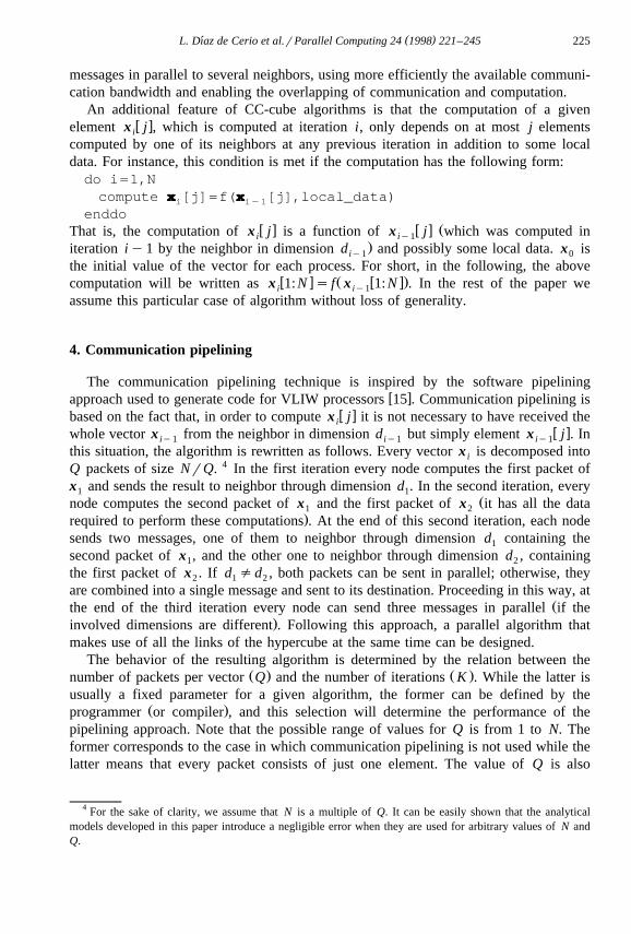
Ž .Fig. 1. An example of communication pipelining. a CC-cube algorithm without communication pipelining.Ž . Ž .b CC-cube algorithm with deep communication pipelining for the example of Qs6. c CC-cube algorithmwith shallow communication pipelining for Qs3.
referred to as the degree of pipelining. The degree of pipelining determines the amountof communication parallelism and computationrcommunication overlapping exploitedby the algorithm.
Two different pipelining schemes are differentiated depending on the value of Q. Thescheme resulting from choosing QGK will be called deep pipelining while the schemederived by selecting Q-K will be referred as shallow pipelining. These schemes aredescribed in detail below.
Ž .Depending on the parameters of the original algorithm N, K , etc. and theŽ .parameters of the architecture communication start-up and bandwidth one of the two
schemes with a particular degree of pipelining will be the most efficient solution.Section 7 presents a method to compute the optimal degree of pipelining.
4.1. Deep pipelining
Deep pipelining is illustrated in Fig. 1. Fig. 1a represents the activity of single nodeof a three dimensional hypercube when executing a CC-cube algorithm with Ks4iterations. The horizontal axis represents time. The computation steps of differentiterations are represented by rectangles with different gray levels. Communications stepsare represented by arrows, also with different gray levels. The order in which the
² :dimension of the hypercube are used for data exchange is 1,2,3,2 . Periods in whichthe node is waiting for data required in the next computation are denoted by w.
Fig. 1b shows the execution flow for deep pipelining. The computation performed atŽ .step i of the original CC-cube algorithm computation of vector x is split into Qi
Ž .packets such that QGK 6 packets in the example of Fig. 1b . Every packet consists ofthe computation of NrQ elements of x . Three phases can be identified in the newi
execution flow. The first phase, which is called the prologue phase, consists of Ky1
( )L. Dıaz de Cerio et al.rParallel Computing 24 1998 221–245´ 227
iterations. In iteration i of the prologue phase, every node computes i packetsŽ .belonging to different computation steps of the original algorithm and sends i packetsto neighbor nodes through dimensions d , d , . . . , d . Packets that use different1 2 i
dimensions are sent in parallel. Those to be sent through the same dimension arecombined into a single message and transmitted to its destination. The next QyKq1iterations form the kernel phase. In every iteration of the kernel phase each nodecomputes K packets and sends them using all the communication links in parallel.Finally, the number of packets computed and sent by every node decreases in each oneof the last Ky1 iterations, which constitute the epilogue phase.
In order to implement deep pipelining, the code executed by every node must berewritten. Being BsNrQ and assuming that QGK , the new code is as follows:do i=1,Ky1do iX=1,ixxxxx X[(iyiX)B+1:(iyiX+1)B]=f(xxxxx X [(iyiX)B+1:(iyiX+1)B])i iy1
enddodo parallel iX=1,iexchange xxxxx X[(iyiX)B+1:(iyiX+1)B] along dimension d Xi i
enddoenddodo i=K,Qdo iX=1,Kxxxxx X[(iyiX)B+1:(iyiX+1)B]=f(xxxxx X [(iyiX)B+1:(iyiX+1)B])i iy1
enddodo parallel iX=1,Kexchange xxxxx X[(iyiX)B+1:(iyiX+1)B] along dimension d Xi i
enddoenddodo i=Q+1,Q+Ky1do iX=iyQ+1,Kxxxxx X[(iyiX)B+1:(iyiX+1)B]=f(xxxxx X [(iyiX)B+1:(iyiX+1)B])i iy1
enddodo parallel iX=iyQ+1,Kexchange xxxxx X[(iyiX)B+1:(iyiX+1)B] along dimension d Xi i
enddoenddoThe code consists of three loops, which correspond to the prologue, kernel and
epilogue phases. For the sake of clarity, the above code ignores the concatenation ofseveral packets into a single message when they are to be sent along the same dimensionof the hypercube.
4.2. Shallow pipelining
Shallow communication pipelining is illustrated in Fig. 1c. Again, every iteration ofthe original algorithm is decomposed into Q packets but unlike deep pipelining, we have
Ž .now that Q-K 3 packets in the example of Fig. 1c . Now, the prologue phase consistsof the first Qy1 iterations. The next KyQq1 iterations are the kernel phase and the
( )L. Dıaz de Cerio et al.rParallel Computing 24 1998 221–245´228
last Qy1 iterations constitute the epilogue phase. In every iteration of the kernel phase,each process sends Q packets using at most Q links in parallel.
Assuming again that BsNrQ, shallow pipelining is implemented by executing thefollowing code at each node:do i=1,Qy1do iX=1,ixxxxx X[(iyiX)B+1:(iyiX+1)B]=f(xxxxx X [(iyiX)B+1:(iyiX+1)B])i iy1
enddodo parallel iX=1,iexchange xxxxx X[(iyiX)B+1:(iyiX+1)B] along dimension d Xi i
enddoenddodo i=Q,Kdo iX=iyQ+1,ixxxxx X[(iyiX)B+1:(iyiX+1)B]=f(xxxxx X [(iyiX)B+1:(iyiX+1)B])i iy1
enddodo parallel iX=iyQ+1,iexchange xxxxx X[(iyiX)B+1:(iyiX+1)B] along dimension d Xi i
enddoenddodo i=K+1,K+Qy1do iX=iyQ+1,Kxxxxx X[(iyiX)B+1:(iyiX+1)B]=f(xxxxx X [(iyiX)B+1:(iyiX+1)B])i iy1
enddodo parallel iX=iyQ+1,Kexchange xxxxx X[(iyiX)B+1:(iyiX+1)B] along dimension d Xi i
enddoenddoCommunication pipelining as described in this section allows to exploit communica-
w xtion parallelism, as shown in 13 . However the overlapping of communication andcomputation cannot be exploited, since the computation steps do not start until all theparallel communications finish.
5. Overlapping communication and computation
This section presents a modification of the pipelined algorithm in order to overlap thecommunication and computation operations.
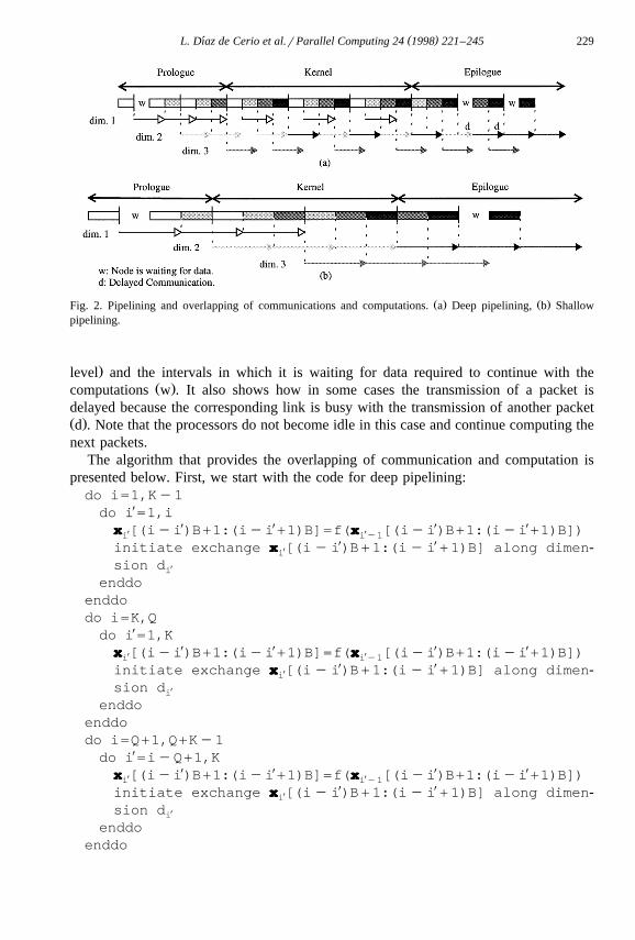
Looking at the pipelined algorithms, we can observe that some packets can be sentbefore the end of the iteration. After a packet is computed it can be sent to its destinationat the same time as the following packet is computed. This overlapping can be applied toboth deep and shallow pipelining in the same way. Fig. 2 shows how the overlappingmethod is applied to the example of Fig. 1. This figure assumes that the transmissiontime of a packet is twice the computation time of the same packet. Fig. 2 shows the
Žintervals in which each node is performing computation rectangles with different gray
( )L. Dıaz de Cerio et al.rParallel Computing 24 1998 221–245´ 229
Ž . Ž .Fig. 2. Pipelining and overlapping of communications and computations. a Deep pipelining, b Shallowpipelining.
.level and the intervals in which it is waiting for data required to continue with theŽ .computations w . It also shows how in some cases the transmission of a packet is
delayed because the corresponding link is busy with the transmission of another packetŽ .d . Note that the processors do not become idle in this case and continue computing thenext packets.
The algorithm that provides the overlapping of communication and computation ispresented below. First, we start with the code for deep pipelining:do i=1,Ky1do iX=1,ixxxxx X[(iyiX)B+1:(iyiX+1)B]=f(xxxxx X [(iyiX)B+1:(iyiX+1)B])i iy1
initiate exchange xxxxx X[(iyiX)B+1:(iyiX +1)B] along dimen-i
sion d Xi
enddoenddodo i=K,Qdo iX=1,Kxxxxx X[(iyiX)B+1:(iyiX+1)B]=f(xxxxx X [(iyiX)B+1:(iyiX+1)B])i iy1
initiate exchange xxxxx X[(iyiX)B+1:(iyiX +1)B] along dimen-i
sion d Xi
enddoenddodo i=Q+1,Q+Ky1do iX=iyQ+1,Kxxxxx X[(iyiX)B+1:(iyiX+1)B]=f(xxxxx X [(iyiX)B+1:(iyiX+1)B])i iy1
initiate exchange xxxxx X[(iyiX)B+1:(iyiX +1)B] along dimen-i
sion d Xi
enddoenddo
( )L. Dıaz de Cerio et al.rParallel Computing 24 1998 221–245´230
We now use the term initiate exchange for describing the fact that the node does notblock after starting the communication but continues with the following computations.
As it was described in Section 4, the first Ky1 iterations of the code for deeppipelining form the prologue phase, the next QyKq1 iterations are the kernel phaseand the last Ky1 constitute the epilogue phase. The nodes do not send the data at theend of every iteration but they send the data after the computation of every packet. Inparallel with the transmission, the nodes compute consecutive packets if they have thenecessary data.
In the case of shallow pipelining, the prologue phase consists of Qy1 iterations, thenext KyQy1 iterations form the kernel phase and the last Qy1 iterations constitutethe epilogue phase. The code executed by each node is as follows:do i=1,Qy1do iX=1,ixxxxx X[(iyiX)B+1:(iyiX+1)B]=f(xxxxx X [(iyiX)B+1:(iyiX+1)B])i iy1
initiate exchange xxxxx X[(iyiX)B+1:(iyiX +1)B] along dimen-i
sion d Xi
enddoenddodo i=Q,Kdo iX=iyQ+1,ixxxxx X[(iyiX)B+1:(iyiX+1)B]=f(xxxxx X [(iyiX)B+1:(iyiX+1)B])i iy1
initiate exchange xxxxx X[(iyiX)B+1:(iyiX +1)B] along dimen-i
sion d Xi
enddoenddodo i=K+1,K+Qy1do iX=iyQ+1,Kxxxxx X[(iyiX)B+1:(iyiX+1)B]=f(xxxxx X [(iyiX)B+1:(iyiX+1)B])i iy1
initiate exchange xxxxx X[(iyiX)B+1:(iyiX +1)B] along dimen-i
sion d Xi
enddoenddo
6. Performance modelling
The choice between deep and shallow pipelining, and more specifically the optimalŽ .degree of pipelining Q , depends on the algorithm–architecture combination. If the
optimal value of Q is lower than K , the shallow pipelining scheme will be used;otherwise, we will choose the deep pipelining approach. In this section, we developanalytical models of the performance of the proposed method that will allow to estimatethe execution time of both pipelining schemes. In addition, analytical models for theoriginal CC-cube algorithm and for the lower bound of the execution time are devel-oped. These models will be used as a reference to evaluate our proposal.
( )L. Dıaz de Cerio et al.rParallel Computing 24 1998 221–245´ 231
An analytical model for the execution time of an algorithm that uses the hypercube² :dimensions in the order given by any arbitrary sequence Ds d , d , . . . , d such1 2 K
that d may be equal to d for some i/ j could be very complex. However, the analysisi j
is much simpler when D is a known sequence because the analysis can be limited tothat particular case. From now on, we will consider the particular case in which
² :Ds d , d , . . . , d such that d /d for all i/ j. Algorithms that use the hypercube1 2 d i j
dimensions in the order given by this sequence do not need to combine more than onepacket into one single message. This particular D is very common in hypercube
Ž .algorithms for example, the Cooley–Tukey algorithm for the FFT problem . This² :particular case can be analyzed without loss of generality assuming Ds 1,2, . . . , d .
Any other permutation of D only needs a renaming of the hypercube dimensions.The parameters of the analytical models can be classified into problem parameters
and architecture parameters. The problem parameters are the following:Ø D: sequence that expresses the order in which the dimensions are usedØ N: number of elements of vector x .iØ S: size of the elements of x .iØ C: average number of operations per element of x .iand the architecture parameters are:Ø d: number of hypercube dimensions.Ø T : computing time per operation.a
Ø T : transmission time per unit size element.e
Ø T : start-up time to initiate a communication through a link.sup
Notice that the higher the ratio ST rCT , the greater the communication overhead.e a
When the ratio ST rCT is high, a reduction in the communication overhead provides ane a
important reduction in the total execution time. So the benefits of our technique will bemore significant in this case.
6.1. Analytical model for the CC-cube algorithm
In each one of the d iterations of a CC-cube algorithm, the whole vector x isi
computed and transmitted through the corresponding dimension. In this way, theexecution time of the original CC-cube algorithm is:
T sd NCT qT qNST . 3Ž .Ž .CC a sup e
6.2. Lower bound of the execution time
In this section, a lower bound on the execution time for any overlapping schemeapplied to a CC-cube algorithm is established. The contribution of the computations tothe execution time is dNCT and the contribution due to start-ups is dT . Thus, we cana sup
obtain an initial lower bound which is equal to the execution time due only to processorŽ .activity. This lower bound is then d NCT qT . Regarding the transmission time,a sup
since the first element of vectors x , x , . . . , x should have been received before1 2 iy1
the first element of vector x can be computed, this element cannot start to be computediŽ .Ž .before iy1 CT qT qST time units. Obviously, the first element of x cannot bea sup e d
( )L. Dıaz de Cerio et al.rParallel Computing 24 1998 221–245´232
Ž .Ž .transmitted before it is computed, it is to say, before dy1 CT qT qST qCT .a sup e a
Because the transmission time of vector x cannot be lower than T qNST thed sup e
execution time of any overlapping scheme based on CC-cube cannot take lower thanŽ .Ž .dy1 CT qT qST qCT qT qNST . According to the above remarks, it isa sup e a sup e
possible to establish the following lower bound:
LBsmax d NCT qT ,d CT qT q Nqdy1 ST . 4Ž . Ž .� 4Ž . Ž .a sup a sup e
6.3. Analytical model for deep pipelining
The analytical model for deep pipelining is obtained by adding the expressionsŽcorresponding to the execution time of the different phases prologue, kernel and
.epilogue of the algorithm.
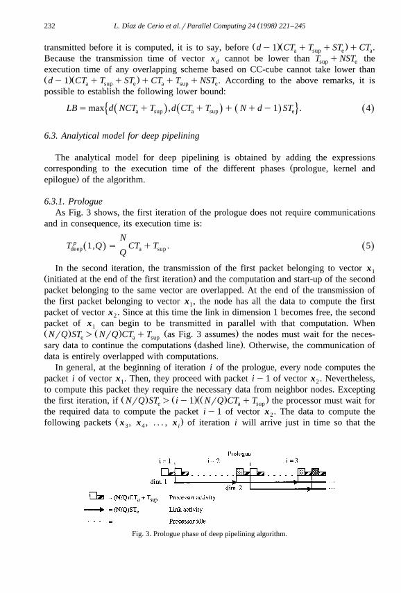
6.3.1. PrologueAs Fig. 3 shows, the first iteration of the prologue does not require communications
and in consequence, its execution time is:
NpT 1,Q s CT qT . 5Ž . Ž .deep a supQ
In the second iteration, the transmission of the first packet belonging to vector x1Ž .initiated at the end of the first iteration and the computation and start-up of the secondpacket belonging to the same vector are overlapped. At the end of the transmission ofthe first packet belonging to vector x , the node has all the data to compute the first1
packet of vector x . Since at this time the link in dimension 1 becomes free, the second2
packet of x can begin to be transmitted in parallel with that computation. When1Ž . Ž . Ž .NrQ ST ) NrQ CT qT as Fig. 3 assumes the nodes must wait for the neces-e a sup
Ž .sary data to continue the computations dashed line . Otherwise, the communication ofdata is entirely overlapped with computations.
In general, at the beginning of iteration i of the prologue, every node computes thepacket i of vector x . Then, they proceed with packet iy1 of vector x . Nevertheless,1 2
to compute this packet they require the necessary data from neighbor nodes. ExceptingŽ . Ž .ŽŽ . .the first iteration, if NrQ ST ) iy1 NrQ CT qT the processor must wait fore a sup
the required data to compute the packet iy1 of vector x . The data to compute the2Ž .following packets x , x , . . . , x of iteration i will arrive just in time so that the3 4 i
Fig. 3. Prologue phase of deep pipelining algorithm.
( )L. Dıaz de Cerio et al.rParallel Computing 24 1998 221–245´ 233
processors do not become idle any more. According to this, the execution time ofiteration i can be calculated by adding the transmission time of the first packet of x iy1Ž . Ž .last packet of iteration iy1 to the processing time computing and start-up time of
Ž . Ž . Ž .ŽŽ . .first packet of x last packet of iteration i . If NrQ ST F iy1 NrQ CT qTi e a sup
the processors do not need to wait for data at any time. In this case, the execution timeof iteration i equals to the processing time of all packets of the iteration.
Thus, the execution time of each one of the dy2 last iterations in the prologue phasecan be expressed as follows:
N NpT i ,Q smax ST , iy1 CT qTŽ . Ž .deep e a sup½ 5ž /Q Q
Nw xq CT qT , ig 2,dy1 . 6Ž .a supQ
The total execution time of the prologue phase can be computed by adding theexecution time of each iteration:
dy1 Np pT Q s T i ,Q s dy1 CT qTŽ . Ž . Ž .Ýdeep deep a supž /Qis1
dy1 N Nq max ST , iy1 CT qT . 7Ž . Ž .Ý e a sup½ 5ž /Q Qis2
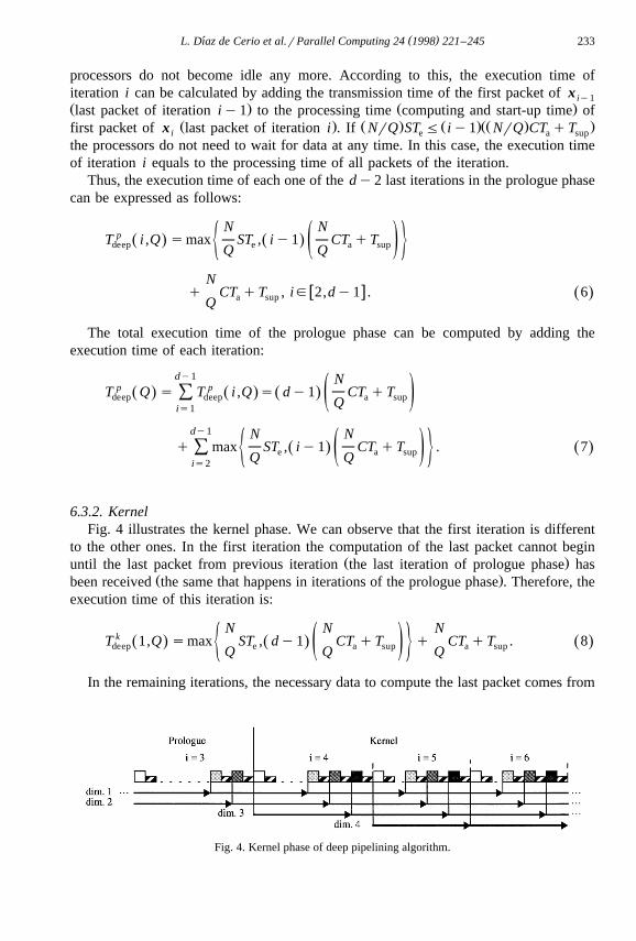
6.3.2. KernelFig. 4 illustrates the kernel phase. We can observe that the first iteration is different
to the other ones. In the first iteration the computation of the last packet cannot beginŽ .until the last packet from previous iteration the last iteration of prologue phase has
Ž .been received the same that happens in iterations of the prologue phase . Therefore, theexecution time of this iteration is:
N N NkT 1,Q smax ST , dy1 CT qT q CT qT . 8Ž . Ž . Ž .deep e a sup a sup½ 5ž /Q Q Q
In the remaining iterations, the necessary data to compute the last packet comes from
Fig. 4. Kernel phase of deep pipelining algorithm.
( )L. Dıaz de Cerio et al.rParallel Computing 24 1998 221–245´234
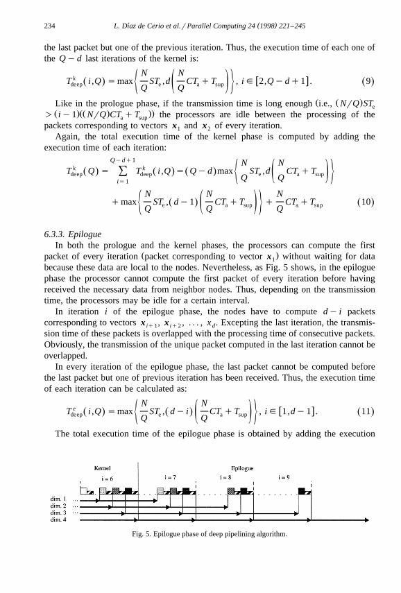
the last packet but one of the previous iteration. Thus, the execution time of each one ofthe Qyd last iterations of the kernel is:
N Nk w xT i ,Q smax ST ,d CT qT , ig 2,Qydq1 . 9Ž . Ž .deep e a sup½ 5ž /Q Q
Ž Ž .Like in the prologue phase, if the transmission time is long enough i.e., NrQ STeŽ .ŽŽ . ..) iy1 NrQ CT qT the processors are idle between the processing of thea sup
packets corresponding to vectors x and x of every iteration.1 2
Again, the total execution time of the kernel phase is computed by adding theexecution time of each iteration:
Qydq1 N Nk kT Q s T i ,Q s Qyd max ST ,d CT qTŽ . Ž . Ž .Ýdeep deep e a sup½ 5ž /Q Qis1
N N Nqmax ST , dy1 CT qT q CT qT 10Ž . Ž .e a sup a sup½ 5ž /Q Q Q
6.3.3. EpilogueIn both the prologue and the kernel phases, the processors can compute the first
Ž .packet of every iteration packet corresponding to vector x without waiting for data1
because these data are local to the nodes. Nevertheless, as Fig. 5 shows, in the epiloguephase the processor cannot compute the first packet of every iteration before havingreceived the necessary data from neighbor nodes. Thus, depending on the transmissiontime, the processors may be idle for a certain interval.
In iteration i of the epilogue phase, the nodes have to compute dy i packetscorresponding to vectors x , x , . . . , x . Excepting the last iteration, the transmis-iq1 iq2 d
sion time of these packets is overlapped with the processing time of consecutive packets.Obviously, the transmission of the unique packet computed in the last iteration cannot beoverlapped.
In every iteration of the epilogue phase, the last packet cannot be computed beforethe last packet but one of previous iteration has been received. Thus, the execution timeof each iteration can be calculated as:
N Ne w xT i ,Q smax ST , dy i CT qT , ig 1,dy1 . 11Ž . Ž . Ž .deep e a sup½ 5ž /Q Q
The total execution time of the epilogue phase is obtained by adding the execution
Fig. 5. Epilogue phase of deep pipelining algorithm.
( )L. Dıaz de Cerio et al.rParallel Computing 24 1998 221–245´ 235
time of each iteration plus the transmission time of the packet computed in the lastiteration:
dy1 dy1 N N Ne eT Q s T i ,Q s max ST , dy i CT qT q ST .Ž . Ž . Ž .Ý Ýdeep deep e a sup e½ 5ž /Q Q Qis1 is1
12Ž .The analytical model for the execution time of the deep pipelining algorithm
corresponds to the addition of the execution time of each one of the previous threephases:
Np k eT Q sT Q qT Q qT Q sd CT qTŽ . Ž . Ž . Ž .deep deep deep deep a supž /Q
N Nq Qyd max ST ,d CT qTŽ . e a sup½ 5ž /Q Q
dy1 N N Nq2 max ST ,i CT qT q ST . 13Ž .Ý e a sup e½ 5ž /Q Q Qis1
6.4. Analytical model for shallow pipelining
The method used to obtain the analytical model for shallow pipelining is similar tothat used for deep pipelining. For short, this section only shows the final result.
The analytical model for shallow pipelining is obtained by adding the execution timeof the prologue, kernel and epilogue phases and results in the following expressions:
N N NT Q sd CT qT q dyQ max ST , Qy1 CT qTŽ . Ž . Ž .shall a sup e a sup½ 5ž / ž /Q Q Q
Qy1 N N Nq2 max ST ,i CT qT q ST . 14Ž .Ý e a sup e½ 5ž /Q Q Qis1
For shallow pipelining, both the prologue and epilogue phases consists in Qy1iterations. Note that the upper limit of the sum in the second term depends on Q. Thekernel phase consists of dyQq1 iterations. This causes that the factor that multipliesthe third term of the expression is dyQ instead of Qyd as it was the case of deeppipelining. We can see that both deep and shallow pipelining schemes are equivalentwhen Qsd, just by evaluating the expressions corresponding to their execution time.
7. Optimal degree of pipelining
Ž .The optimal degree of pipelining Q depends on the algorithm–architecture combi-nation. An increase on Q produces an increase on the amount of communications thatare overlapped with computations. Nevertheless, an increase on Q produces an increaseon the number of packets to transmit, that is to say, a higher number of star-up
( )L. Dıaz de Cerio et al.rParallel Computing 24 1998 221–245´236
operations, which cannot be overlapped with computations. Our objective in this sectionis to determine the optimal degree of pipelining, that is, the value of Q that minimizesthe execution time. We consider separately the evaluation of the optimal degree of
Ž .pipelining when using shallow pipelining Q and when using deep pipeliningshall_optŽ .Q . Once Q and Q have been obtained, the analytical expressionsdeep_opt shall_opt deep_opt
developed in Section 6 allows us to select the optimal scheme to minimize thecommunication overhead.
w xSince for shallow pipelining, Qg 1, dy1 , the cost of an exhaustive search toŽ .obtain Q is O d . Since d is a small number for real machines, we can afford toshall_opt
w xanalyze the whole interval 1, dy1 . In this case, the optimal degree of pipelining canbe expressed as:
<w x w xQ s Q g 1,dy1 T Q FT Q ,;Qg 1,dy1 . 15� 4Ž . Ž . Ž .shall_opt 0 shall 0 shall
Ž .The cost of an exhaustive search to obtain Q is O N because it is necessarydeep_optw xto analyze all values in the interval d, N , which is the interval of possible values for
Q, when using deep pipelining. In this section, we propose a search strategy that isŽ .O d .
Ž .The objective is to find the value of Q that minimizes T Q . The analyticaldeepŽ .expression for T Q was introduced at the end of Section 6.3. What makes difficultdeep
to work with this expression is the presence of the max operator in the second and thirdŽ .terms. We can rewrite T Q in such a way that the max operator is eliminated. Todeep
Ž . Ž . ŽŽ .that propose we define j Q as the value of i which makes NrQ ST F i NrQ CT qe a.T , that is:sup
NSTe NSTQ e
j Q s s . 16Ž . Ž .N NCT qQTa supCT qTa supQ
Ž .We can then rewrite the third term of T Q as follows:deep
Ž .j Q y1dy1 dy1N N N N2 max ST ,i CT qT s2 ST q i CT qT .Ý Ý Ýe a sup e a sup½ 5ž / ž /ž /Q Q Q Qis1 is1 Ž .isj Q
17Ž .Ž .According to this, the analytical expression of T Q can be expressed in terms ofdeep
Ž .j Q without using the max operator, as follows:
T QŽ .deep
N N°Qqdy1 ST qd CT qT , if j Q )d ;Ž . Ž .e a supž /Q Q~s
N N22 j Q y1 ST q Qdy j Q q j Q CT qT , if j Q Fd.Ž . Ž . Ž . Ž .Ž . Ž .e a sup¢ ž /Q Q
18Ž .
( )L. Dıaz de Cerio et al.rParallel Computing 24 1998 221–245´ 237
Ž . Ž .The analytical minimization of T Q is still difficult due to the presence of j Q .deepw xWe decompose now the interval d, N of possible values for Q into dq1 intervals I ,i
Ž . Ž . w xin such a way that j Q s i a constant for all the values of Q within I for ig 1, d .i
The definition of I is slightly different. I is defined as the interval of values of Qdq1 dq1Ž .such that j Q )d. To be precise, the intervals I are defined as follows:i
<w x w x w xI s p ,q ; d , N j Q )d ,;Qg p ,q ; 19� 4Ž . Ž .dq1 dq1 dq1 dq1 dq1
<w x w x w x w xI s p ,q ; d , N j Q s i ,;Qg p ,q ,; ig 1,d . 20� 4Ž . Ž .i i i i i
Ž . Ž . Ž .Notice that p q -p q because j Q decreases as Q increases.i i iy1 iy1Ž . Ž .Inside the interval I the expression T Q does not depend on j Q . Inside thedq1 deepŽ . Ž . Ž .intervals I , with iFd, the expression T Q depends on j Q but j Q keepsi deep
constant. Thus, given an interval I , and assuming Q as a real number, we can obtain theiŽ .optimal pipelining degree inside the interval by deriving the expression T Q . Wedeep
will call Q the optimal pipelining degree inside each interval. For the interval I thei dq1Ž .expression T Q is decreasing so we have that:deep
Q sq . 21Ž .dq1 dq1
For I , with iFd, we have that:i
° 2 2p , if l -p ;i i
2 2~l, if p FlFq ;Q s 22Ž .i ii
2 2¢q , if q -l ,i i
where:
22 iy1 NST y i y i NCTŽ . Ž .e als . 23Ž .) dTsup
According to the above results, the optimal pipelining degree of deep pipelining is:
<w x w xQ s Q ,ig 1,dq1 T Q FT Q ,; jg 1,dq1 24Ž . Ž .� 4Ž .deep_opt i dee p i dee p j
8. Performance figures
This section shows some performance figures based on the analytical modelsdescribed in Section 6. These figures come from the application of the overlapping
Žmethod to two different CC-cube algorithms. The first algorithm computes the FFT Fast.Fourier Transform based on the decimation-in-frequency algorithm of Cooley–Tukey
w x d16 . The second algorithm computes a Vector Add, which performs the addition of 2vectors, each one stored in one of the hypercube nodes. At the end of the Vector Addevery node has a copy of the resulting vector. The main difference between these twoproblems is the ratio SrC, that is to say, the relative weight of communications andcomputations. To be precise, the FFT problem needs to perform Cs10 operations foreach element to be transmitted. Taking into account that the elements are complex
( )L. Dıaz de Cerio et al.rParallel Computing 24 1998 221–245´238
Ž .numbers Ss2 it results in SrCs0.2. The Vector Add problem only needs toperform one operation for each element to be transmitted. Since the elements are realnumbers, in this case we have that SrCs1. The higher the ratio SrC, the moreimportant the communication overhead reduction since the communication componentof the algorithm is more dominant.
Next, we describe these two problems in more detail and then we present someperformance figures. In the case of the FFT, we compare the performance of our
w xapproach with that proposed by Johnson and Krawitz in 7 and the approach proposedw xby Aykanat and Dervis in 5 .
8.1. FFT
The literature about algorithms for FFT is very extensive. One of the most popularw xand efficient algorithms is the Cooley–Tukey 16 , which can be executed on a
w x w xhypercube following the approach described in 7 and 5 among others. This parallelimplementation of the Cooley–Tukey is a particular example of a CC-cube algorithm.
The CC-cube algorithm is as follows. Assume we have to compute the FFT of asequence of 2 n complex numbers. Each node of the d-dimensional hypercube will storeinitially 2 ny d complex numbers. The algorithm consists in n stages. In each of the firstnyd stages every node performs a certain computation without any data exchange. Thiscomputation consists in 2 ny dy1 butterflies. Every butterfly takes two complex numbersof the sequence and produces two complex numbers of a new sequence. A butterflyrequires six real additions and four real products. In each of the d last stages of thealgorithm, every node computes also 2 ny dy1 butterflies but, at the end of each stage,
Ž ny dy1every node exchanges half of the values computed by these butterflies 2 complex.numbers with one of its neighbors in the hypercube. The order in which the dimensions
of the hypercube are used during these d stages is Ds-d, dy1, . . . , 1) . Followingthe previously introduced notation, in this CC-cube algorithm we have that Ksd;vectors x consist in Ns2 ny dy1 complex numbers; the size of every elementiŽ .complex number is Ss2; and the number of real operations per element of x isi
Cs10.The computation performed by every node satisfies the requirements for communica-
tion pipelining. That is, to perform the jth butterfly of stage nydq i, node q onlyrequires one of the complex numbers produced by itself in the jth butterfly of stagenydq iy1 and one of the complex numbers produced by its neighbor along dimen-sion dy iq1, also in the jth butterfly of stage nydq iy1.
The execution time of the CC-cube algorithm and the lower bound can be computedby adding the computing cost of the initial nyd stages, which do not requirecommunication, to the expressions derived in Sections 6.1 and 6.2. That gives thefollowing expressions:
T s nyd 10NT qd 10NT qT q2 NT ; 25Ž . Ž .Ž .CC a a sup e
LBs nyd 10NT qmax d 10NT qT ,d 10T qT q Nqdy1 2T .Ž . Ž .� 4Ž . Ž .a a sup a sup e
26Ž .
( )L. Dıaz de Cerio et al.rParallel Computing 24 1998 221–245´ 239
w xJohnson and Krawitz proposed in 7 an adaptation of the Cooley–Tukey FFT tohypercube multicomputers. The method is based on the communication pipeliningtechnique, but it does not exploit the possibility of overlapping communications andcomputations. They proposed to split the vectors of data in N packets of one elementeach. It is to say, QsN. We will call this technique full communication pipelining. Thefirst nyd stages are computed locally to the processors. The last d stages are computedin Nqdy1 steps. The first dy1 steps form the prologue phase, the Nydq1following steps form the kernel phase and the last dy1 steps form the epilogue phase.In the ith step of the prologue phase every processor computes i butterflies andexchanges i data in parallel along i dimensions of the hypercube. In every step of thekernel phase, every processor computes d butterflies and exchanges d data in parallelalong all the dimensions of the hypercube. Finally in the ith step of the epilogue phaseevery node computes dy i butterflies and exchanges dy i data in parallel along dy idimensions of the hypercube. Thus, the execution time of the algorithm proposed byJohnson and Krawitz can be expressed as:
T sn10NT qNdT q Nqdy1 2T . 27Ž . Ž .JoKr a sup e
w xAykanat and Dervis proposed in 5 a method to overlap communications andcomputations to solve the FFT problem using the Cooley–Tukey algorithm. In each ofthe last d stages of the algorithm every node compute 2 ny d complex data. Half of thesedata are transmitted to the neighbor node in one of the hypercube dimensions and theremaining data stay local to the node. Aykanat and Dervis propose to compute the datato be transmitted in first place and then, to compute the local data. The local data arecomputed at the same time that the previous data are transmitted. Every butterfly needsten real operations to produce two complex numbers. The first complex number can beobtained after eight real operations. After two more operations the second number datais obtained. Therefore, the communications are overlapped only with a fifth part of thecomputations. The execution time of the Aykanat–Dervis algorithm is given by thefollowing expression:
� 4T s nyd 10NT qd 8 NT qT qdmax 2 NT ,2 NT . 28Ž . Ž .Ž .AyDe a a sup a e
8.2. Vector Add
The second problem to be considered is the sum of 2 d vectors of size N. Everyvector is stored in a different hypercube node. At the end, every node must have a copyof the resulting vector. Many parallel algorithms for solving linear algebra problems usethe Vector Add computation as an step. Some examples are Householder transforma-tions for QR decomposition and one-sided Jacobi methods for singular value decomposi-
w xtion and eigenvalue computation 17 .A CC-cube algorithm for this problem consists of d stages. In iteration i, every node
exchange a copy of the updated vector with the neighbor node through dimension i.After the exchange, the received vector is added to the local vector to obtain the newupdated vector. This algorithm meets the necessary conditions to apply the communica-tions pipelining technique.
( )L. Dıaz de Cerio et al.rParallel Computing 24 1998 221–245´240
²The dimensions of the hypercube are used in the following sequence: Ds 1, 2, . . . ,: Ž .d . The elements of the vectors are real numbers Ss1 and the number of operations
Ž .to compute each element is one Cs1 .The main reason to choose Vector Add as a second example is that the contribution
of the communications to the total execution time is more important in this problem thanin the FFT. Therefore, the Vector Add problem provides a better scenario so that theproposed method achieves more important reductions in the communication overhead,even for small values of T .e
We will assume that the total number of data element is also 2 n. Due to the fact thatthe whole vector x must be transmitted to a neighbor node at every stage, the numberi
of elements to transmit per stage is Ns2 ny d. Notice that, unlike the FFT, all iterationshave communication and computation steps.
The analytical models for the CC-cube algorithm and the lower bound LB are theones presented in Sections 6.1 and 6.2.
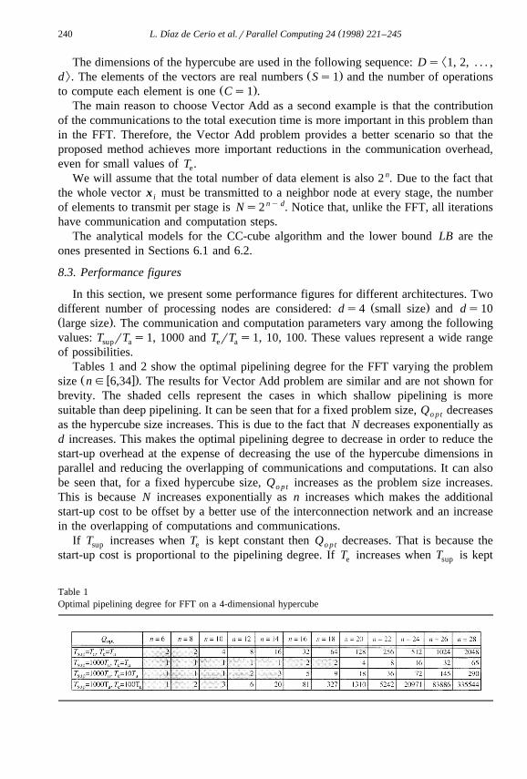
8.3. Performance figures
In this section, we present some performance figures for different architectures. TwoŽ .different number of processing nodes are considered: ds4 small size and ds10
Ž .large size . The communication and computation parameters vary among the followingvalues: T rT s1, 1000 and T rT s1, 10, 100. These values represent a wide rangesup a e a
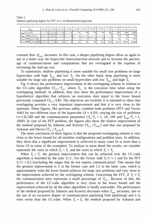
of possibilities.Tables 1 and 2 show the optimal pipelining degree for the FFT varying the problemŽ w x.size ng 6,34 . The results for Vector Add problem are similar and are not shown for
brevity. The shaded cells represent the cases in which shallow pipelining is moresuitable than deep pipelining. It can be seen that for a fixed problem size, Q decreaseso p t
as the hypercube size increases. This is due to the fact that N decreases exponentially asd increases. This makes the optimal pipelining degree to decrease in order to reduce thestart-up overhead at the expense of decreasing the use of the hypercube dimensions inparallel and reducing the overlapping of communications and computations. It can alsobe seen that, for a fixed hypercube size, Q increases as the problem size increases.o p t
This is because N increases exponentially as n increases which makes the additionalstart-up cost to be offset by a better use of the interconnection network and an increasein the overlapping of computations and communications.
If T increases when T is kept constant then Q decreases. That is because thesup e o p t
start-up cost is proportional to the pipelining degree. If T increases when T is kepte sup
Table 1Optimal pipelining degree for FFT on a 4-dimensional hypercube
( )L. Dıaz de Cerio et al.rParallel Computing 24 1998 221–245´ 241
Table 2Optimal pipelining degree for FFT on a 10-dimensional hypercube
constant then Q increases. In this case, a deeper pipelining degree allow us again too p t
use in a better way the hypercube interconnection network and to increase the percent-age of communications and computations that are overlapped at the expense ofincreasing the start-up cost.
To summarize, shallow pipelining is more suitable for small size problems on largehypercubes with high T and low T . On the other hand, deep pipelining is moresup e
suitable for large size problems on small hypercubes with low T and high T .sup e
Fig. 6 shows the performance improvement of the overlapping scheme in relation toŽthe CC-cube algorithm T rT , where T is the execution time when using theCC ov ov
.overlapping method . In addition, they also show the performance improvement of ahypothetical algorithm that achieves an execution time equal to the lower bound
Ž .previously computed T rLB . The objectives are twofold: it is intended to show thatCC
overlapping provides a very important improvement and that it is very close to theŽoptimum. These figures, like previous tables, combine both problems FFT and Vector
. Ž .Add for two different sizes of the hypercube ds4,10 , varying the size of problemsŽ w x. Žng 6,34 and the communication parameters T rT s1, 10, 100 and T rT s1,e a sup a
.1000 . In case of the FFT problem, the figures also show the relative improvement ofŽ .the method proposed by Johnson and Krawitz T rT and that one proposed byCC JoKr
Ž .Aykanat and Dervis T rT .CC AyDe
The main conclusion of these figures is that the proposed overlapping scheme is veryclose to the lower bound for all machine configurations and problem sizes. In addition,
Žthey show that a significant improvement is achieved in many cases it is more than a.factor 10 in some of the examples . To analyze in more detail the results, we consider
separately the cases in which T sT and the cases in which T )T .e a e a
When T sT the greatest improvement that can be achieved over the CC-cubee a
algorithm is bounded by the ratio SrC. For the Vector Add SrCs1 and for the FFTŽ .SrCs0.2 excluding the stages that do not require communication . This means that
the greatest improvement is 2 in the former case and 1.2 in the latter case, which isapproximately what the lower bound achieves for large size problems and very close tothe improvement achieved by the overlapping scheme. Concerning the FFT, if T sTe a
the communication time represents a small percentage of T . Because of this, theCC
performance of the CC-cube algorithm is very close to the lower bound and theimprovement achieved by all the other algorithms is hardly noticeable. The performanceof the method proposed by Johnson and Krawitz decreases when T increases, due tosup
Ž .the use of an excessive degree of communication pipelining full pipelining and it iseven worse than the CC-cube. When T sT the method proposed by Aykanat ande a
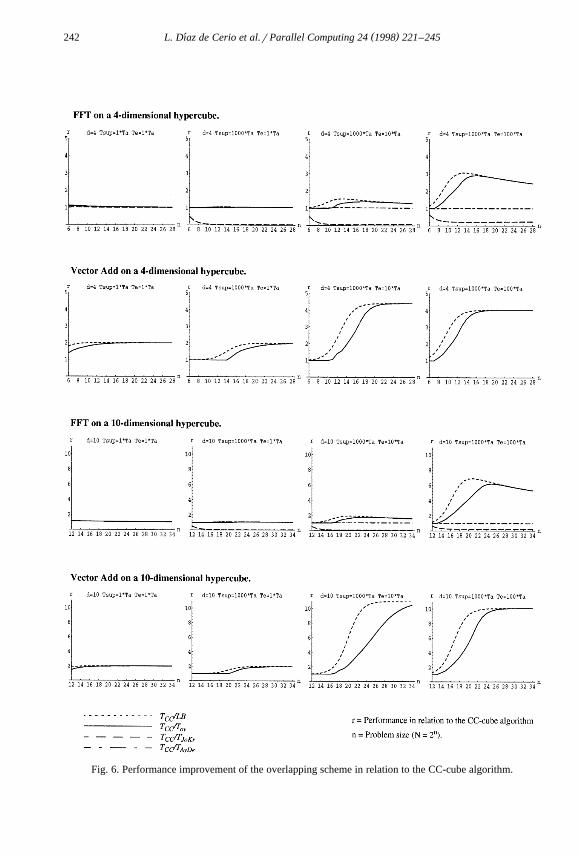
( )L. Dıaz de Cerio et al.rParallel Computing 24 1998 221–245´242
Fig. 6. Performance improvement of the overlapping scheme in relation to the CC-cube algorithm.
( )L. Dıaz de Cerio et al.rParallel Computing 24 1998 221–245´ 243
Dervis achieves a full overlapping of the communication time. Nevertheless, as saidbefore, the greatest improvement that can be achieved by any overlapping algorithm isbounded by 1.2.
When T )T the communication time represents a more important part of the T .e a CC
In this case, any reduction of the communication overhead becomes an importantreduction of the total execution time. For Vector Add, if T is higher enough than T , thee a
improvement of the overlapping scheme over the CC-cube algorithm can be slightlyŽ .more than d for high values of n d is the hypercube dimension . In this case, the
communication is the dominant cost and our scheme reduces the execution time byusing the d links in parallel and overlapping computations with communications. Theimprovement for the FFT is not so high because the ratio ST rCT is lower for the FFTe a
than for Vector Add. Moreover, the FFT problem has some stages without anycommunication that represent a high percentage of the total execution time when n ishigh. In any case, notice that when T )T the improvements obtained with the methode a
proposed by Aykanat and Dervis are always very low. The reason is that this methoddoes not use the hypercube dimensions in parallel and at most one fifth of thecomputation can be overlapped with communication. The method proposed by Johnsonand Krawitz gets better when the ratio T rT grows because the reduction in thee sup
communication time is more noticeable. Nevertheless, the full pipelining is still exces-sive. In fact, the full pipelining is only recommended when T 4T , but this is note sup
usual in current multicomputers. On the other hand, the figures obtained with themethod proposed in this paper are always close to those corresponding to the lowerbound.
9. Conclusions
This paper presents a method to reduce the execution time of a kind of parallelŽ .algorithms CC-cube algorithms on hypercubes. The method can be applied under the
assumption that every hypercube node can communicate through d links in parallel andcan also overlap these communications with computations. Thus, it is necessary thatevery node has d communication controllers that can be used in parallel with theprocessing unit of the node.
The proposed method is based on the communication pipelining technique. Thistechnique reorganizes the computations so that the d controllers and the processing unitcan be used in parallel, unlike the CC-cube algorithm, in which all of these devices areused in a serial way. As a result, an important reduction in the communication overheadis achieved. If computations are dominant on the execution time of the CC-cubealgorithm, this reduction is obtained essentially by the overlapping of communicationsand computations. On the other hand, when communications are the dominant factor, thereduction in the communication overhead is mainly obtained by using the d links inparallel. The main features of the proposed overlapping method are as follows.
Ø It is a method that can be applied to a wide range of algorithms for hypercubes. Inthe literature, there are particular solutions to specific problems that are difficult to adaptto other problems. We have illustrated the method by means of two real problems: FFT
( )L. Dıaz de Cerio et al.rParallel Computing 24 1998 221–245´244
and Vector Add. There are many other problems on which the method can be applied.We are working presently on the following problems: Fast Harley Transform, Jacobimethods for single value decomposition and eigenvalue computation and All-to-Allcommunication problems.
Ø The method automatically chooses the optimal pipelining degree for a givenproblem and a given architecture. The pipelining degree determines the amount ofcommunications and computations that are overlapped but also the start-up overhead. Itis shown by means of two examples that the proposed method achieves a performancevery close to the optimum. Other proposals in the literature, besides being particularsolutions to a specific problem, can vary neither the degree of pipelining nor the amountof overlapping and therefore the performance of the algorithm is much lower than thatof our scheme, for some machine configurations.
Ø The reduction in execution time may be very important in some cases. Forinstance, in the examples used in the paper, a reduction of a factor of more than 10 isachieved for some machine configurations.
Acknowledgements
This work has been supported by the Ministry of Education and Science of SpainŽ . Ž .CICYT TIC-95r0429 and the European Center for Parallelism in Barcelona CEPBA .
References
w x1 W.C. Athas, C.L. Seitz, Multicomputers: Message—Passing Concurrent Computers, IEEE ComputerŽ .1988 9–24.
w x2 G. Fox et al., Solving Problems on Concurrent Processors, Prentice-Hall, Englewood Cliffs, NJ, 1988.w x3 F. Thomson Leighton, Introduction to Parallel Algorithms and Architectures: Arrays, Trees and Hyper-
cubes, Morgan Kaufmann Publishers, 1992.w x4 R.C. Agarwal, F.G. Gustavson, M. Zubair, An Efficient Algorithm for the 3-D FFT NAS Parallel
Ž .Benchmark, Scalable High-Performance Computing Conference 1994 129–133.w x5 C. Aykanat, A. Dervis, An Overlapped FFT Algorithm for Hypercube Multicomputers, International
Ž .Conference on Parallel Processing 1991 III-316–III-317.w x6 M.J. Clement, M.J. Quinn, Overlapping computations, communications and IrO in parallel sorting, J.
Ž .Parallel Distributed Comput. 28 1995 162–172.w x Ž .7 S.L. Johnson, R.L. Krawitz, Cooley–Tukey FFT on the connection machine, Parallel Comput. 18 1992
1201–1221.w x8 A. Sahay, Hiding Communication Costs in Bandwidth-Limited Parallel FFT Computation, Report:
UCBrCSD 93r722, University of California, 1993.w x9 A. Suarez, C. Ojeda-Guerra, Overlapping Computations and Communications in Tours Networks, 4th´
Ž .Euromicro Workshop on Parallel and Distributed Processing 1996 .w x10 C. Aykanat, A. Dervis, Efficient fast Hartley transform algorithms for hypercube-connected multicomput-
Ž . Ž .ers, IEEE Trans. Parallel Distributed Syst. 6 6 1995 561–577.w x11 S.L. Johnson, C.T. Ho, Optimum broadcasting and personalized communication in hypercubes, IEEE
Ž .Trans. Comput. 38 1989 1249–1268.w x12 M. Mantharam, P.J. Eberlein, Block recursive algorithm to generate Jacobi-sets, Parallel Comput. 19
Ž .1993 481–496.
( )L. Dıaz de Cerio et al.rParallel Computing 24 1998 221–245´ 245
w x13 L. Dıaz de Cerio, A. Gonzalez, M. Valero-Garcıa, Communication pipelining in hypercubes, Parallel´ ´ ´Ž . Ž .Processing Lett. 6 4 1996 507–523.
w x14 L. Dıaz de Cerio, M. Valero-Garcıa, A. Gonzalez, Overlapping Communication and Computation in´ ´ ´Ž .Hypercubes, Second International Euro-Par Conference, Vol. 1 1996 253–257.
w x15 M. Lam, Software Pipelining: An Effective Scheduling Technique for VLIW machines, Conf. onŽ .Programming Language Design and Implementation 1988 318–328.
w x16 J.C. Cooley, J.W. Tukey, An algorithm for the machine computation of complex Fourier series, Math.Ž .Comp. 19 1965 291–301.
w x17 G.H. Golub, C.F. Van Loan, Matrix Computations, The Johns Hopkins University Press, 1983.
Related Documents