A measurement of_diffusion_in_47_tucanae

A MEASUREMENT OF DIFFUSION IN 47 TUCANAE

Jeremy Heyl1, Harvey B. Richer1, Elisa Antolini2, Ryan Goldsbury1, Jason Kalirai3,4, Javiera Parada1, andPier-Emmanuel Tremblay3

1 Department of Physics and Astronomy, University of British Columbia, Vancouver, BC V6T 1Z1, Canada; [email protected], [email protected] Dipartimento di Fisica e Geologia, Università degli Studi di Perugia, I-06123 Perugia, Italia

3 Space Telescope Science Institute, Baltimore MD 21218, USA4 Center for Astrophysical Sciences, Johns Hopkins University, Baltimore MD, 21218, USA; [email protected]

Received 2015 February 6; accepted 2015 February 20; published 2015 April 30

ABSTRACT

Using images from the Hubble Space Telescope Wide-Field Camera 3, we measure the rate of diffusion of starsthrough the core of the globular cluster 47 Tucanae (47 Tuc) using a sample of young white dwarfs that wereidentified in these observations. This is the first direct measurement of diffusion due to gravitational relaxation. Wefind that the diffusion rate k » -10 13 arcsec2 Myr−1 is consistent with theoretical estimates of the relaxation timein the core of 47 Tuc of about 70Myr.

Key words: globular clusters: individual (47 Tuc) – Hertzsprung–Russell and C–M diagrams – stars: kinematicsand dynamics – stars: Population II

1. INTRODUCTION

Globular clusters have long provided an amazing laboratoryfor stellar evolution and gravitational dynamics, and the nearbyrich cluster, 47 Tuc (47 Tuc), has long been a focus of suchinvestigations. The key point of this investigation is theinterplay between these two processes. In particular, in the coreof 47 Tuc, the timescale for stellar evolution and the timescalefor dynamical relaxation are similar. The relaxation time in thecore of 47 Tuc is about 70Myr (Harris 1996). Meanwhile overa span of about 150Myr, the most massive stars in 47 Tucevolve from a red giant star with a luminosity of 2000 timesthat of the Sun to a white dwarf (WD) with a luminosity lessthan a tenth that of the Sun. Meanwhile the star loses about40% of its mass, going from 0.9 to 0.53 solar masses. It is theseyoung WDs that are the focus of this paper.

Although the core of 47 Tuc has been the focus of numerousprevious investigations (e.g., McLaughlin et al. 2006; Kniggeet al. 2008; Bergbusch & Stetson 2009), this is the first paperthat combines the near-ultraviolet filters of the Hubble SpaceTelescope (HST) with a mosaic that covers the entire core ofthe cluster. Probing the core of the cluster in the ultraviolet isadvantageous in several ways. First, the young WDs areapproximately as bright as the upper main-sequence, giant, andhorizontal branch stars at 225 nm, so they are easy to find. Infact the brightest WDs are among the brightest stars in thecluster and are as bright as the blue stragglers. Second, thepoint-spread function of HST is more concentrated in theultraviolet helping, with confusion in the dense starfield that isthe core of 47 Tuc.

In spite of these advantages, for all but the brightest stars,our data set suffers from incompleteness, which presents someunique challenges. We reliably characterize the incompletenessas a function of position and flux in the two bands of interest,F225W and F336W, throughout the color–magnitude diagram(CMD) and especially along the WD cooling sequence throughthe injection and recovery of about 108 artificial stars into theimages. How we measure the completeness is described indetail in Section 3.1. The young WDs typically have a mass40% less than their progenitors, so they are born with lesskinetic energy than their neighbors, and two-body interactions

will typically increase the kinetic energy of young WDs overtime and change their spatial distribution. We introduce asimple model for the diffusion of the young WDs through thecore of the cluster (Section 3.2). To make the most of thisunique data set, we have to include stars in our sample whosecompleteness rate is well below 50%. We have developed andtested statistical techniques to characterize the observationaldistribution of young WDs in flux and space to understand theirmotion through the cluster and their cooling (Sections 3.4–3.7)in the face of these potentially strong observational biases.Although these techniques are well-known especially ingamma-ray astronomy, they have never been applied to stellarpopulations in this way, so Section 3.8 presents a series ofMonte Carlo simulations to assess the potential biases of thesetechniques and verify that these techniques are indeed unbiasedin the face of substantial incompleteness within the statisticaluncertainties. To establish the time over which the WDs dimwe use a stellar evolution model outlined in Section 3.3.Section 4 describes the best-fitting models for the density andflux evolution of the WDs. Section 4.1 looks at the dynamicconsequences of these results. Section 5 outlines futuredirections both theoretical and observational and the broaderconclusions of this work.

2. OBSERVATIONS

A set of observations from the Advanced Camera forSurveys (Ford et al. 1998) and the Wide Field Camera 3(WFC3, MacKenty 2012) on the HST of the core of theglobular cluster 47 Tuc over 1 yr provides a sensitive probe ofthe stellar populations in the core of this globular cluster (Cycle12 GO-12971, PI: Richer), especially the young WDs. Here wewill focus on the observations with WFC3 in the UV filtersF225W and F336W. The observations were performed over tenepochs from 2012 November to 2013 September. Each of theexposures in F225W was 1080 s, and the exposures in F336Wwere slightly longer at 1205 s. Each of the overlapping WFC3images was registered onto the same reference frame anddrizzled to form a single image in each band from which starswere detected and characterized, resulting in the CMD depictedin Figure 1.

The Astrophysical Journal, 804:53 (11pp), 2015 May 1 doi:10.1088/0004-637X/804/1/53© 2015. The American Astronomical Society. All rights reserved.

1

What is immediately striking in Figure 1 is that thedistribution of young WDs with a median age of 6Myr issignificantly more centrally concentrated than that of the olderWDs that have a median age of 127Myr. The WD distributionappears to become more radially diffuse with increasing age, asignature of relaxation. One concern is immediately apparent.The numbers of observed stars are given in the legend of theleft panel and the numbers of stars in the completenesscorrected samples are given in the legend of the right panel.The sample of older WDs is only about 75% complete onaverage. Furthermore, one would expect the completeness ofthese faint stars to be lower near the center of the cluster, so ifthe completeness is not accounted for correctly, one couldnaturally conclude that the WDs are diffusing when in realitythey are not. In principle we would like to divide this sample ofover 1,300 stars into subsamples, some of which will have evensmaller completeness rates. How can we be sure that ouranalysis techniques are up to the task of measuring thisdiffusion accurately in the face of completeness rates as low as20% that vary dramatically with distance from the center of thecluster?

In Section 3 we will characterize the completeness ratethrough artificial star tests, and develop and test statisticaltechniques to measure the diffusion of WDs in 47 Tucwithout binning the stars at all, thus preserving the maximuminformation content of these data. We will test these newalgorithms on mock data sets that include both thecompleteness rate and flux error distribution of our sampleto verify that they robustly determine the diffusion and fluxevolution of the WDs. The subsequent section (Section 4)

explores results of these techniques on the data set depictedin Figure 1.

3. ANALYSIS

3.1. Artificial Star Tests

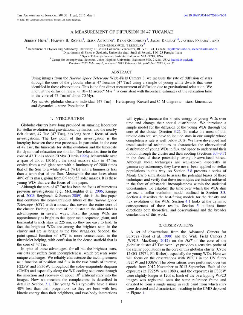
We inserted ~108 artificial stars into the WFC3 images inF225W and F336W over the full range of observed magnitudesin both bands and a range of distances from the center of thecluster. To determine the completeness rate for the WDs thatwe have observed, we inserted artificial stars whose F225Wand F336W magnitudes lie along the observed WD track in theCMD. The rate of recovering a star along the WD track of agiven input magnitude in F336W at a given radius is thecompleteness rate and is depicted in Figure 2. If an artificial staralong the WD track is detected in F336W, it is always detectedin F225W as well. The completeness rate is both a strongfunction of radius and magnitude and is significantly differentfrom unity except for the brightest stars, so accounting forcompleteness robustly is crucial in the subsequent analysis. Theradial bins are 100 pixels in width and the magnitude bins are0.1358 wide.The magnitudes of the recovered stars give the error

distribution as a function of the input magnitude and positionof the star in the field. Furthermore, these distributions are nottypically normal and often asymmetric as well. For the analysisin Section 3.5 we use the cumulative distribution of magnitudeerrors as a function of position and input magnitude, which weobtain by sorting the output magnitudes in a given bin andspline to obtain the cumulative distribution in the form of the

Figure 1. Left: color–magnitude diagram of the core of 47 Tuc in the WFC3 filters F225W and F336W. Right: the radial distribution of young and old white dwarfstars as highlighted in the color–magnitude diagram (completeness corrected numbers appear in the right panel).

2

The Astrophysical Journal, 804:53 (11pp), 2015 May 1 Heyl et al.

values of the errors from the first to the ninety-ninth percentile.In the analysis the completeness rate is interpolated over thetwo dimensions of radius and magnitude with a third-degreespline, and the error distributions are interpolated linearly overthe three dimensions (radius, magnitude, and percentile).

3.2. Diffusion and Luminosity Evolution

Sometime during the late evolution of a turn-off star in47 Tuc, the star loses about 40% of its mass, going from amain-sequence star of 90% of a solar mass to a WD of 53% of asolar mass (Renzini & Fusi Pecci 1988; Renzini et al. 1996;Moehler et al. 2004; Kalirai et al. 2009). These newborn WDswill have the typical velocities of their more massiveprogenitors, so as they interact gravitationally with other stars,their velocities will increase through two-body relaxation,bringing their kinetic energies into equipartition (e.g., Spit-zer 1987). Because the gravitational interaction is long-rangeand the distance between the stars is small compared to the sizeof the cluster, the change in velocity will be dominated bydistant interactions and small random velocity jumps, i.e., theCoulomb logarithm is large, ~ Nln , where N is the number ofstars in the core of the cluster, ~ -105 6. These small jumps invelocity can be modeled as a random walk in velocity so thesquare of the velocity increases linearly in time and the

relaxation time can be defined as = éëê

ùûú-

t d v dtln .r2 1

In thecenter of the cluster, the density of stars is approximatelyconstant, so the gravitational potential has the approximateform

f r= πG r23

. (1)c2

By the virial theorem the mean kinetic energy of the WDs willequal the mean potential energy,

r=v πG r12

23

(2)c2 2

so the square of the distance of the WDs from the center of thecluster will also increase linearly with time as a random walk;therefore, let us suppose that newly born WDs diffuse outwardthrough the cluster following the diffusion equation

rk r

¶¶

=r tt

r t( , )

( , ), (3)2

where κ can be related to the relaxation time as k = r tc r2

because =d r dt d v dtln ln2 2 from Equation (2). Thisdiffusion equation yields the Green’s function

k= k-u r t

π te( , )

1

8( )(4)r t

3 2(4 )2

if κ is independent of time and position. This gives acumulative distribution in projected radius

< = - k-C R e( ) 1 . (5)R t(4 )2

The Green’s function at t = 0 is a delta function centered on thecenter of the cluster. On the other hand, if the initial distributionis a Gaussian centered on the center of the cluster the density ofWD stars near the center of the cluster is a function of age, t,and projected radius, R, of the form

r rk k

= =+

é

ëêê - +

ù

ûúúR t

Rt t

Rt t

( , )2

4 ( )exp

4 ( )(6)

0

2

0

where the density distribution is normalized as

ò r =¥

R t dR( , ) 1. (7)0

The dispersion of the Gaussian at t = 0 is simply given bys k= t2 42

0. Because the diffusion equation is linear, a sum ofseveral Gaussians with the same value of κ but differentnormalizations and values of t0 will also be a solution.Of course we do not directly observe the ages of the WDs.

Rather we observe their fluxes or apparent magnitudes. Thecooling curve of the WDs is a relationship between time andthe apparent magnitude from the WDs t(m), so the number ofWDs that we expect to observe at a given flux and radius isgiven by

r=¶¶

f R m N R t mtm

C R m( , ) ˙ ( , ( )) ( , ), (8)

where N is the birthrate of the WDs (assumed to be constantover the range of ages of the young WDs, i.e., the past200Myr) and C R m( , ) is the completeness as a function ofradius and flux. To this point flux errors have been neglected.

3.3. Cooling Models

To construct the various cooling models here, i.e., t(m) fromEquation (8), we used Modules for Experiments in StellarAstrophysics (MESA; Paxton et al. 2011) to performsimulations of stellar evolution starting with a pre-main-sequence model of 0.9 solar masses and a metallicity of= ´ -Z 3.3 10 3 appropriate for the cluster 47 Tuc. This is

slightly larger than the value for the turnoff mass found byThompson et al. (2010) for the eclipsing binary V69 in 47 Tucthat is composed of an upper main sequence star of about 0.86solar masses and a subgiant of 0.88 solar masses. Because weare interested in the stars that have become young WDs justrecently, the initial masses of these stars should be slightlylarger than the turnoff mass today. We have explicitly assumedthat the progenitors of the WDs are a uniform population.Although there is evidence of modest variation in the chemicalabundances in 47 Tuc (e.g., Milone et al. 2012), the WDcooling sequence, at least at larger radii, appears uniform(Richer et al. 2013). However, from Figure 1 it is apparent that

Figure 2. Completeness rate as a function of radius from the center of 47 Tucand the magnitude of the artificial star.

3

The Astrophysical Journal, 804:53 (11pp), 2015 May 1 Heyl et al.

the core of 47 Tuc has a substantial population of bluestragglers that will evolve to become more massive WDs. Oursample has about 160 blue stragglers, and if we estimate theduration of the main-sequence for a blue straggler to be1–2 Gyr (e.g., Sills et al. 2009), we obtain a birth-rate of blue-straggler WDs of about 0.1 Myr−1. The number of giants in ourfield indicates a birth rate of about eight WDs per million years(see Goldsbury et al. 2012 for further details), so the estimatedcontamination of the WD cooling sequence is modest atabout 1%.

Specifically, we used SVN revision 5456 of MESA andstarted with the model 1 M_pre_ms_to_wd in the testsuite. We changed the parameters initial_mass andinitial_z of the star and adjusted the parameterlog_L_lower_limit to −6 so the simulation would runwell into the WD cooling regime. We also reduced the twovalues of the wind η to 0.46 (from the default of 0.7) to yield a0.53 solar mass WD from the 0.9 solar mass progenitor.Interestingly Miglio et al. (2012) argue from Kepler aster-oseismic measurements of the stars in the metal-rich opencluster NGC 6971 that such values of η are needed to accountfor the mass loss between the red giant and red clump phases ofstars in this metal-rich cluster.

We defined the time of birth of the WD to coincide with thepeak luminosity of the model at the tip of the asymptotic giantbranch about 10.9 Gyr after the start of the simulation. This isin agreement with the best age of the cluster determined frommain-sequence stars of 11.25± 0.21 (random) ±0.85 (sys-tematic) Gyr (Thompson et al. 2010). This age agrees with thatderived by Hansen et al. (2013) from WD cooling(9.9± 0.7 Gyr at 95% confidence). We choose this definitionof the birth so that each observed WD will have a star of similarluminosity in the cooling model. At this point in the evolutionwe have outputs from the MESA evolution every 100 yr or so;therefore, the cooling curve is well-sampled throughout. Ateach output time we have the value of the luminosity, radius,effective temperature, and mass of the star. With these valueswe interpolate the spectral models of Tremblay et al. (2011) insurface gravity and effective temperature, and then scale theresult to the radius of the model star. We use a true distancemodulus of 13.23 (Thompson et al. 2010) and a reddening of

- =E B V( ) 0.04 (Salaris et al. 2007) to determine the modelfluxes in the WFC3 band F336W. We used the standardextinction curve of Fitzpatrick (1999) with

- =A E B V( ) 3.1V . We have purposefully used a distanceand reddening determined from main-sequence stars to avoid apotential circularity in using the WD models themselves to fixthe distance. Woodley et al. (2012) inferred a slightly largertrue distance modulus of 13.36 0.02 0.06 from the WDspectral energy distributions.

The brightest WD in our sample has F336W = 14.92.According to the models this corresponds to an age of110,000 yr, an effective temperature of 100,000 K, a luminosityof 1600 Le, and a radius of 0.13 Re. Its mass is 0.53 solarmasses. The faintest WD in our sample has F336W = 25.4,yielding an age of 1.2 Gyr, an effective temperature of 8700 K,a luminosity of 10−3 Le, and a radius of 0.013 Re, one-tenth ofthe radius of the brightest WD. Clearly the brightest WD in oursample is not a WD in the usual sense because thermal energyplays an important role in the pressure balance of the star. Forthis brightest star =glog 5.93, which is less than the minimumof the atmosphere model grid ( =glog 6) so we have to

extrapolate slightly off of the grid, but only for this brighteststar. For the simulations in Section 3.8 we did not use thisparticular model, but similar ones of the same WD mass withdifferent neutrino cooling rates or initial metallicities alsogenerated with MESA.

3.4. Likelihood Function

The model outlined in Section 3.2 predicts the number ofWDs as a function of magnitude and position. Let us divide thespace of position and magnitude into bins of widthDR andDmwhere the bins are numbered with indices j and k, respectively.The probability of finding n stars in a particular bin is given by

=éëê D D ù

ûú- D D

( )( )( ) ( )

P n f R m

f R m R m e

n

; ,

,

!. (9)

j k

j kn f R m R m,j k

Now we imagine dividing the sample into so many bins thatthere is either a single star in a bin or no stars at all; we have

=

´ìíïï

îïï

D D

- D D( )( )( )

( )P n f R m e

f R m R m

; ,

, one star

1 no star. (10)

j kf R m R m

j k

,j k

We can define the likelihood as the logarithm of the product ofthe probabilities of observing the number of stars in each bin.Since the bins are so small we can replace Rj and mk for thebins with stars in them with the measured values for thatparticular star Ri and mi. This gives the so-called “unbinnedlikelihood” of observing the sample as follows (Cash 1979;Mattox et al. 1996; Davis 2014):

å å= - D D( )( )L f R m f R m R mlog log , , . (11)i

i ij k

j k,

We have dropped the constant widths of the bins from the firstterm, which is a sum over the observed stars; consequently, theabsolute value of the likelihood is not important, justdifferences matter. The second term is a sum over the reallynarrow (and arbitrary) bins that we have defined, so we have

òå D D = =( ) ( )f R m R m f R m dRdm N, , , (12)j k

j k j k,

pred

where Npred is the number of stars that the model predicts thatwe will observe, so finally we have

å= -( )L f R m Nlog log , , (13)i

i i pred

where the summation is over the observed stars. The integralfor Npred when combined with Equation (8) yields

ò ò r=N N R t C R m dRdt˙ ( , ) ( , ) (14)t r

pred0 0

1 max

or

ò ò r=N N R t C R mdtdm

dRdm˙ ( , ) ( , ) . (15)m

m r

pred00

1 max

4

The Astrophysical Journal, 804:53 (11pp), 2015 May 1 Heyl et al.

If we take the luminosity function as fixed and try to maximizethe likelihood with respect to the diffusion model

å r=é

ëêê

¶¶

ù

ûúú -( ) ( )L N R t m

tm

C R m Nlog log ˙ , ( ) , (16)i

ii

i i pred

å

å

r= éë

ùû

+é

ëê궶

ù

ûúú -

( )

( )

N R t m

tm

C R m N

log ˙ , ( )

log , , (17)

ii

i ii i pred

where the second summation does not depend on the diffusionmodel, so it is constant with respect to changes in the diffusionmodel and can be dropped from the logarithm of the likelihood.However, it must be included if one wants to compare differentcooling curves, t(m).

3.5. Magnitude Errors

An important complication to the analysis is that themeasured magnitudes are not the same as the actual magnitudesof the stars; in particular the error distribution is not normal oreven symmetric. This transforms the model distributionfunction via a convolution,

ò¢ = ¢ ¢ - ¢ ¢-¥

¥f R m f R m g R m m m dm( , ) ( , ) ( , , ) (18)

ò

ò

= - D - D D D

= - D

-¥

¥f R m m g R m m m d m

f R m m dG

( , ) ( , , ) ( )

( , ) , (19)0

1

where

òD = - D D ¢ D ¢-¥

DG R m m g R m m m d m( , , ) ( , , ) ( ) (20)

m

is the cumulative distribution of magnitude errors with theobserved radius and magnitude fixed. If we calculate thepercentiles of the magnitude error distribution as Dm j we canapproximate the integral as the sum

å¢ = - D( )f R m f R m m( , )1

100, , (21)

jj

so for a given star i we have

år¢ = - D

´ ¢ - D - D

( )( )

( ) ( )

( )f R m N R t m m

t m m C R m m

, ˙ ,

, , (22)

i ij

i j

i j i i j

where ¢ = ¶ ¶t t m. This new function ¢f R m( , )i i can besubstituted into Equation (13) to yield a likelihood includingthe magnitude errors. We will assume that the magnitude errorsdo not affect our estimate of Npred; this simplifies the analysis.We will verify our technique with Monte Carlo simulations inSection 3.8.

3.6. Constraining the Luminosity Function

We can construct a maximum likelihood estimator of theluminosity function of the WDs or alternatively the cooling

curve as follows

r= =¶¶

f R mdN

dmdRN R t

tm

( , ) ˙ ( , ) (23)

år d= -N R t A m m˙ ( , ) ( ), (24)i

i i

where i is an index that runs over the observed stars. With thismodel we can define a likelihood function for the stars that weobserve

å r= éë

ùû -( )L NA R t Nlog log ˙ , , (25)

ii i i pred

where a multiplicative constant (infinite in this case) and thecompleteness for each star have been dropped from thelogarithm.Substituting the trial luminosity function Equation (23)

yields

òå r= ( ) ( )N A N R t C R m dR˙ , , . (26)i

i

r

i ipred0

max

If we maximize the likelihood with respect to the values of Ak

we obtain

r r¶ éë

ùû

¶=

¶ éë

ùû

¶¶¶

( ) ( ) ( )R t C R m

A

R t

t

t

A

log , , log ,, (27)

i i i i

k

i i

i

i

k

where

¶¶

=>⩽{t

Ak ik i

1 if0 if

(28)i

k

so

å

å

r

r

¶ éë

ùû

¶

= +¶ é

ëùû

¶⩾

( ) ( )

( )

A R t C R m

A

A

R t

t

log , ,

1 log ,(29)

i

i i i i i

k

k i k

i i

i

and

rk

¶¶

=+

-+

R tt

R

t t t tlog[ ( , )]

4 ( )

1. (30)

2

02

0

Taking the derivative of Npred yields the second part of thevariance in Llog ,

ò

òå

r

r

¶

¶=

+¶

¶¶¶

( ) ( )

( ) ( )

N

AN R t C R m dR

A NR t

t

t

AC R m dR

˙ , ,

˙ ,, (31)

k

r

k k

ii

r i

i

i

ki

pred

0

0

max

max

ò

òå

r

r

=

+¶

¶⩾

( ) ( )( ) ( )

N R t C R m dR

A NR t

tC R m dR

˙ , ,

˙ ,, . (32)

r

k k

i ki

r i

ii

0

0

max

max

5

The Astrophysical Journal, 804:53 (11pp), 2015 May 1 Heyl et al.

Combining these results with ¶ ¶ =L Alog 0k yields anequation of the form

ò

òå

r

r

r

=

é

ëêêê

¶

¶

-¶ é

ëùû

¶

ù

û

úúú

⩾

( ) ( )

( ) ( )

( )

AN R t C R m dR

A NR t

tC R m dR

R t

t

1 ˙ , ,

˙ ,,

log ,(33)

k

r

k k

i ki

r i

ii

i i

i

0

0

max

max

or a matrix equation of the form

å = +M A bA1

, (34)i

ik i kk

where

=ìíïïîïï <

⩾M

M i ki k

if0 if

(35)iki

and

òr

=¶

¶( ) ( )M NR t

tC R m dR˙ ,

, . (36)i

r i

ii

0

max

The vector bk is given by

ò

år

r

=¶ é

ëùû

¶-

´

⩾

( )

( ) ( )

bR t

tN

R t C R m dR

log ,˙

, , . (37)

ki k

i i

i

r

k k0

max

Although this matrix equation has as many rows as there arestars in the sample, it is straightforward to solve at leastformally in two ways. The first is

=å -

AM A b

1(38)k

i ik i k

and the second is

=+

-+

=+

-+ +

-

+

-

( )( )

( )

Ab A

M

b A

M

Ab A

M

,

. (39)

ii i

i

i i

i

nn i

n

11 1

1

1

1

The values of bi and Mi depend on the values of Ai through theparameter tk, so the solution must proceed iteratively whileminimizing with respect to the other parameters of the model κand t0.

For each value of the diffusion parameters, we chose toiterate Equation (38) three times to determine the values of Akwithin a loop of two iterations whereMi (Equation (36)) and bk(Equation (37)) vary. Given this new trial luminosity function,the diffusion parameters are varied to find the maximumlikelihood, and the iterative solution of the luminosity functionis repeated. These two steps are repeated until the values of thediffusion parameters from one iteration to the next havechanged by less than one part per hundred.

An interesting limit is when the density distribution isindependent of time. This understandably yields a simpler

solution for Ai. In particular, Mi = 0 so

ò r= - =éëêê

ùûúú

-

( ) ( )Ab

N R m C R m dR1 ˙ , , , (40)i

i

r

i i0

1max

where the underlying density distribution is normalized. Theweight is not the reciprocal of the completeness for star i butrather the reciprocal of the mean of the completeness of a starwith the flux of star i over the density distribution. The lattercould be evaluated by taking the mean of the completenessmeasured for all the stars in the sample in a magnitude rangeabout star i sufficiently wide to sample the density distribution.It is important to note that the weight is the reciprocal of themean of the completeness not the mean of the reciprocal. If thecompleteness does not depend strongly on radius, these twowill approximately coincide. Finally if the density distributionis not known a priori and is not modeled, the weight for aparticular star is simply given by = -[ ]A C R m( , )i i i

1. We callthis “Inv Comp” in Figures 6 and 10.The likelihood is invariant under changes in the birth rate of

the WDs (N ) if one also changes the values of k A, i and t0 asfollows:

a a a k ak- -N N A A t t˙ ˙ , , and . (41)i i1

01

0

That is, the timescale cannot be fixed without some additionalinput such as a theoretical cooling curve or an independentestimate of the WD birthrate. The quantities A Ni , k N , and Nt˙ 0

are invariant with respect to this transformation. In our data setwhen we use this modeling technique, we fix the value of N tothe value inferred by the number of giants in our field as inGoldsbury et al. (2012).

3.7. Constraining the Luminosity Function with Errors

We start the analysis including magnitude errors withEquations (18) and (24), which when combined yield

ò år d¢ = ¢ ¢ -

´ ¢ - ¢ ¢

-¥

¥( )f R m N R t C R m A m m

g R m m m dm

( , ) ˙ ( , ) ( , )

( , , ) (42)i

i i

å r= -( ) ( )N A R t g R m m m˙ , , , . (43)i

i i i i

With this model we can define a likelihood function for thestars that we observe

å å r=é

ëêê -

´ ùûú -

( ) ( )

( )

L N A R t g R m m m

C R m N

log log ˙ , , ,

, . (44)

j ii j i j i j i

j i pred

Note how the magnitude error essentially translates into aspread in the age of the observed stars

åå

r

r

dr

¶¶

=ìíïïï

îïïï

-

-

´é

ë

êêê

+¶ é

ëùû

¶

ù

û

úúú

üýïïï

þïïï-

¶

¶

⩾

( ) ( ) ( )( ) ( ) ( )

( )

LA

R t g R m m m C R m

A R t g R m m m C R m

AR t

t

N

A

log , , , ,

, , , ,

log ,. (45)

k j i k

j i j i j i j i

l l j l j l j l j l

ik ii i

i k

,

pred

6

The Astrophysical Journal, 804:53 (11pp), 2015 May 1 Heyl et al.

Although we have included this additional complication in thederivations for completeness, we have found that the inclusionof error convolution in modeling simulated data does not affectthe fitting results, so we did not include this in the modeling ofthe dynamics while simultaneously determining the luminosityfunctions.

3.8. Monte Carlo Simulations

To test these techniques in the face of the challenges ofincompleteness and magnitude errors present in our data, wetypically simulated on the order of 10,000 catalogs of the samesize as our data set with a known luminosity function and aknown diffusion model and attempted to recover the inputparameters. In both cases, the age of the star is first selected tobe between zero and 1.5 Gyr. Given this age the model coolingcurve determines the F336W magnitude. Second, a radius isselected from the cumulative distribution in projected radius(Equation (5)). Given the radius and magnitude of thecandidate for the catalog, the completeness for this star iscalculated and the star is included in the sample with thisprobability. Finally, the magnitude errors are applied bydrawing from the magnitude error distribution. We created asample of 3167 stars—the same as in the WFC3 WD sample.The fitting procedure followed two different strategies.

The first was to assume a fixed cooling curve and try to findthe density evolution to determine whether the process is biasedin determining the diffusion parameters and the typical errors.Finally, we performed simulations where we did not convolvethe models with the error distribution to calculate the likelihood(in all cases errors were applied to the simulated data) to seewhether the omission of this step introduced biases. The secondstrategy did not assume a cooling curve and determined thecooling curve as a part of the process of determining thediffusion. We did not convolve the cooling curve with the errordistribution while fitting the model; however, the fake catalogswere created in the same way as in the first strategy. In thistechnique the resulting cooling curve can be multiplied by aconstant factor (Equation (41)), so we determine the values ofκ and t0 by fixing the value of N to the one used to build thecatalog. This also fixes the age estimates of all of the WDs inthe sample.

The results of these simulations are depicted in Figures 3 and4 and in Table 1. The key results of the simulations are that thelikelihood fitting of the diffusion model results in an unbiasedestimate of the diffusion parameters regardless of whether thefitting technique includes the magnitude errors (Section 3.5).Furthermore, even when one fits for the luminosity function aswell one can obtain reliable estimates of the diffusion modelwithout prior knowledge of the cooling curve; of course, in thislatter case the timescales of the diffusion rely on anindependent estimate of the birth rate of the WDs N .Observationally, this is determined from a sample of giantstars numbering in the thousands (see Figure 1) so thestatistical error in this determination is small. Typically thebirth rate is recovered with an uncertainty of less than 1% andthe diffusion rate with an uncertainty of 10% and t0 with anuncertainty of 15%. The errors in t0 and κ are correlated so theerror in kt0 is typically less than 10%.

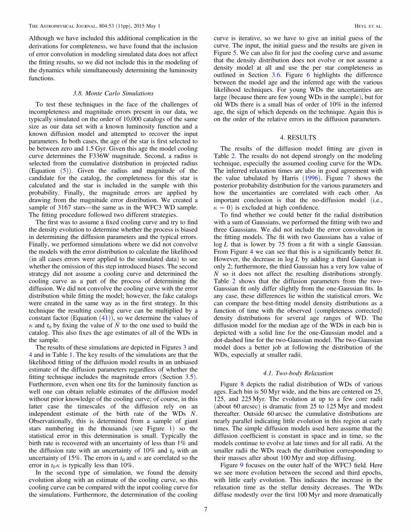
In the second type of simulation, we found the densityevolution along with an estimate of the cooling curve, so thiscooling curve can be compared with the input cooling curve forthe simulations. Furthermore, the determination of the cooling

curve is iterative, so we have to give an initial guess of thecurve. The input, the initial guess and the results are given inFigure 5. We can also fit for just the cooling curve and assumethat the density distribution does not evolve or not assume adensity model at all and use the per star completeness asoutlined in Section 3.6. Figure 6 highlights the differencebetween the model age and the inferred age with the variouslikelihood techniques. For young WDs the uncertainties arelarge (because there are few young WDs in the sample), but forold WDs there is a small bias of order of 10% in the inferredage, the sign of which depends on the technique. Again this ison the order of the relative errors in the diffusion parameters.

4. RESULTS

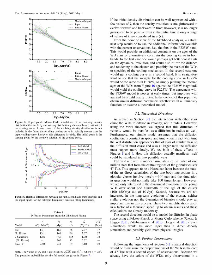
The results of the diffusion model fitting are given inTable 2. The results do not depend strongly on the modelingtechnique, especially the assumed cooling curve for the WDs.The inferred relaxation times are also in good agreement withthe value tabulated by Harris (1996). Figure 7 shows theposterior probability distribution for the various parameters andhow the uncertainties are correlated with each other. Animportant conclusion is that the no-diffusion model (i.e.,k = 0) is excluded at high confidence.

To find whether we could better fit the radial distributionwith a sum of Gaussians, we performed the fitting with two andthree Gaussians. We did not include the error convolution inthe fitting models. The fit with two Gaussians has a value of

Llog that is lower by 75 from a fit with a single Gaussian.From Figure 4 we can see that this is a significantly better fit.However, the decrease in Llog by adding a third Gaussian isonly 2; furthermore, the third Gaussian has a very low value ofN so it does not affect the resulting distributions strongly.Table 2 shows that the diffusion parameters from the two-Gaussian fit only differ slightly from the one-Gaussian fits. Inany case, these differences lie within the statistical errors. Wecan compare the best-fitting model density distributions as afunction of time with the observed (completeness corrected)density distributions for several age ranges of WD. Thediffusion model for the median age of the WDs in each bin isdepicted with a solid line for the one-Gaussian model and adot-dashed line for the two-Gaussian model. The two-Gaussianmodel does a better job at following the distribution of theWDs, especially at smaller radii.

4.1. Two-body Relaxation

Figure 8 depicts the radial distribution of WDs of variousages. Each bin is 50Myr wide, and the bins are centered on 25,125, and 225Myr. The evolution at up to a few core radii(about 60 arcsec) is dramatic from 25 to 125Myr and modestthereafter. Outside 60 arcsec the cumulative distributions arenearly parallel indicating little evolution in this region at earlytimes. The simple diffusion models used here assume that thediffusion coefficient is constant in space and in time, so themodels continue to evolve at late times and for all radii. At thesmaller radii the WDs reach the distribution corresponding totheir masses after about 100Myr and stop diffusing.Figure 9 focuses on the outer half of the WFC3 field. Here

we see more evolution between the second and third epochs,with little early evolution. This indicates the increase in therelaxation time as the stellar density decreases. The WDsdiffuse modestly over the first 100Myr and more dramatically

7

The Astrophysical Journal, 804:53 (11pp), 2015 May 1 Heyl et al.

during the second 200Myr. The WDs as expected fromtheoretical considerations suffer diffusion that is a function ofradius and time and beyond the scope of the simple model usedto quantify the diffusion in this paper. However, this modeldoes capture the diffusion within a few core radii for a few corerelaxation times.

5. CONCLUSIONS

5.1. Further Analysis

In this paper we used the Green’s function (Equation (4)) tomodel the diffusion of the stars through the cluster. We simplytook the initial conditions to be a Gaussian or a sum ofGaussians centered on the center of the cluster. This allowedfor a simple closed-form expression for the density function inspherical coordinates and in projection as well. Withoutrelaxing the spherical symmetry one could imagine muchmore general initial conditions. In fact we have an estimate ofthe initial conditions in the form of the projected radialdistribution of the stars on the upper main-sequence. Thisdistribution could be possibly deprojected as a lowered-isothermal distribution in phase space (Michie 1963;King 1966) and convolved with the Gaussian Green’s function,Equation (4), to give the expected density distribution as afunction of time. This technique shares the advantage of thetechnique used in this paper that the density distribution can beguaranteed to be positive because the convolution of thepositive kernel with a positive distribution is necessarilypositive; however, the density distribution even in sphericalcoordinates is not available in closed form.

A second strategy would be to expand the initial densitydistribution in terms of spherical Bessel functions and sphericalharmonics. If we restrict ourselves to an initially sphericaldistribution we have

òr = k¥

-r t dka k ekr

kr( , ) ( )

sin ( ), (46)k t

0

2

where the coefficients a(k) are determined from the initialdensity distribution

ò r=¥

a kπ

dr kr rkr

kr( )

2( ) ( , 0)

sin ( ). (47)

0

2

Figure 3. Upper panel: the values of the fitted parameters are typicallyunbiased with respect to the input values in the simulations. Here N is depicted.The input values for the two types of simulations are given by the vertical lines.Lower panel: the values of t0.

Figure 4. Upper panel: the values of the fitted parameters are typicallyunbiased with respect to the input values in the simulations. Here κ is depicted.The input values for the two types of simulations are given by the vertical lines.Lower panel: the distribution of Llog is significantly wider when errorconvolution is included in the fitting process.

Table 1Parameters from the Monte Carlo Simulations: Means, Standard Derivations,

Input Values

Technique κ Input t0 Input

Full Modeling 3.4 ± 0.3 3.58 560 ± 80 531No-error Convolution 3.7 ± 0.4 3.71 530 ± 80 515Unfixed LF 7.5 ± 0.6 7.26 220 ± 30 231

N Input Llog

Full Modeling 5.42 ± 0.03 5.44 ±50No-error Convolution 5.45 ± 0.03 5.45 ±22Unfixed LF L ±20 L

8

The Astrophysical Journal, 804:53 (11pp), 2015 May 1 Heyl et al.

If the initial density distribution can be well represented with afew values of k, then the density evolution is straightforward toevolve forward and backward in time; however, it is no longerguaranteed to be positive even at the initial time if only a rangeof values of k are considered in a (k).From the point of view of the likelihood analysis, a natural

next step would be to use the additional information availablewith the current observations, i.e., the flux in the F225W band.This would provide an additional constraint on the ages of theWD stars or alternatively constrain the cooling curve in bothbands. In the first case one would perhaps get better constraintson the dynamical evolution and could also fit for the distanceand reddening to the cluster, and possibly the mass of the WDsor specifics of the cooling mechanism. In the second case onewould get a cooling curve in a second band. It is straightfor-ward to see that the weights for the cooling curve in F225Wwould be the same as in F336W, so simply plotting the inferredages of the WDs from Figure 10 against the F225W magnitudewould yield the cooling curve in F225W. The agreement withthe F336W model is poorer at early times, but improves withage and lasts until nearly 1 Gyr. In the context of this paper, weobtain similar diffusion parameters whether we fit a luminosityfunction or assume a theoretical model.

5.2. Theoretical Directions

As argued in Section 3.2 the interactions with other starscause the WDs to diffuse in velocity, not in radius. However,using the virial theorem we argued that this diffusion invelocity would be manifest as a diffusion in radius as well.Furthermore, our simple model assumes that the diffusioncoefficient is constant in space and time when in fact with timethe WD distribution approaches that of stars of similar mass sothe diffusion must cease and also at larger radii the diffusionmust happen more slowly. We see both of these effects inFigures 8 and 9. How this diffusion actually manifests itselfcould be simulated in two possible ways.The first is direct numerical simulation of on order of one

million stars that form the central regions of the globular cluster47 Tuc. This appears to be a Herculean labor because the state-of-the-art direct calculation of the two body interactions in aglobular cluster involve merely ~105 stars and the simulationin question would normally take 100 times longer. However,we are only interested in the dynamical evolution of the youngWDs over about one hundredth of the age of the cluster(100–150Myr out of 10 Gyr). Second, because we are notinterested in the long-term evolution of the cluster, neitherstellar evolution nor the dynamics of binaries should play animportant role in this process. These two simplifications resultin a factor of a thousand speed up to obtain results and thesecalculations are already underway.The second direction would be to model the diffusion in phase

space using a Fokker–Planck or Monte Carlo scheme (Giersz &Heggie 2011; Pattabiraman et al. 2013; Hong et al. 2013). Suchsimulations would be more rapid than a direct N-bodysimulations and possibly yield more physical insights.

5.3. Further Observations

Following the arguments of Section 5.2 a natural directionwould be to measure the proper motions of the WDs in the coreof 47 Tuc with a second epoch of observations. Because wealready have the colors of the WDs, only observations in a

Figure 5. Upper panel: Monte Carlo simulations of an evolving densitydistribution that are fit by an evolving distribution yield an unbiased estimate ofthe cooling curve. Lower panel: if the evolving density distribution is notincluded in the fitting the resulting cooling curve is typically steeper than theinput cooling curve; however, this difference is subtle. The initial guess is thestarting point for the iterative solution of the cooling curve.

Figure 6. Relative differences between the first, second, and third quartiles andthe input model for the different luminosity function fitting techniques.

Table 2Diffusion Parameters from the Likelihood Fitting

κ t0 s0 N t r( )r c

Model (( )2 Myr−1) (Myr) (″) (Myr−1) (Myr)

Full 13.1 166 66 7.07 37No Errors 13.1 166 66 7.07 372 Gaussians 12.8 14.9 19.5 1.90 38(No Errors) L 260 82 5.32 LFree LF 9.80 241 69 8.10 49

Note. The values of s0 and tr are given by kt2 0 and krc2 , where =r 22c .

The posterior probabilities for the full model are given in Figure 7.

9

The Astrophysical Journal, 804:53 (11pp), 2015 May 1 Heyl et al.

single band would be required and possibly not as deep as thepresent set of observations because the stars have already beendetected. To obtain the most precise positions and to minimizethe crowding, the bluest band would be best, i.e., F225W, andpossibly over only a portion of the field of the current data,

because here the goal would be to verify the current result byfinding the corresponding signal in velocity space, so a fullsample of 3000 plus WDs may not be required.

5.4. Final Remarks

We have measured directly for the first time the dynamicalrelaxation of stars in a globular cluster. To do this we haveintroduced new statistical techniques for the characterization ofstellar populations. These techniques can robustly andstraightforwardly account for high incompleteness and non-Gaussian magnitude errors. They can be applied to a widevariety of questions from globular cluster dynamics to galaxyluminosity functions. There are many avenues for furtherinvestigation, such as a more thorough analysis of the existingdata using the information from the second band, thesimulation of the relaxation of young WDs in numericalmodels, and measuring the proper motions of the young WDsto search for signatures of relaxation in their velocities as well.

Figure 7. Posterior probabilities of the best-fitting parameters. The upper panels depict the covariance among the various parameters. The contours trace probabilities afactor of e, e2, and e3 smaller than the maximum likelihood. The color scale also gives the natural logarithm of the relative likelihood. The lower panels give thelikelihood as a function of a single parameter with the other parameters integrated out.

Figure 8. Radial distribution of white-dwarf samples of various age ranges andmedian ages (given in parenthesis) and the best-fitting two-Gaussian diffusionmodels superimposed. The core radius from Harris (1996) is depicted by thevertical line.

Figure 9. Radial distribution of white-dwarf samples of various age ranges andmedian ages (given in parenthesis) and the best-fitting two-Gaussian diffusionmodels superimposed for the outer half of the region.

Figure 10. Flux in the WFC3 band F336W as a function of time since the peakluminosity of the star that we define to be the birth of the “white dwarf.” Themodel curve assumes a true distance modulus of 13.23 (Thompson et al. 2010)and a reddening of - =E B V( ) 0.04 (Salaris et al. 2007). The “Inv Comp”’technique ignores the effects of diffusion in modeling the stars and uses thecompleteness rate corresponding to the observed magnitude and radius ofeach star.

10

The Astrophysical Journal, 804:53 (11pp), 2015 May 1 Heyl et al.

This research is based on NASA/ESA Hubble SpaceTelescope observations obtained at the Space TelescopeScience Institute, which is operated by the Association ofUniversities for Research in Astronomy Inc. under NASAcontract NAS5-26555. These observations are associated withproposal GO-12971 (PI: Richer). This work was supported byNASA/HST grant GO-12971, the Natural Sciences andEngineering Research Council of Canada, the CanadianFoundation for Innovation, and the British Columbia Knowl-edge Development Fund. This project was supported by theNational Science Foundation (NSF) through grant AST-1211719. It has made used of the NASA ADS and arXiv.org.

REFERENCES

Bergbusch, P. A., & Stetson, P. B. 2009, AJ, 138, 1455Cash, W. 1979, ApJ, 228, 939Davis, D. 2014, Likelihood Tutorial, http://fermi.gsfc.nasa.gov/ssc/data/

analysis/scitools/likelihood_tutorial.html, accessed: 2014–08-11Fitzpatrick, E. L. 1999, PASP, 111, 63Ford, H. C., Bartko, F., Bely, P. Y., et al. 1998, in SPIE Conf. Ser. 3356, Space

Telescopes and Instruments V, ed. P. Y. Bely, & J. B. Breckinridge(Bellingham, WA: SPIE), 234

Giersz, M., & Heggie, D. C. 2011, MNRAS, 410, 2698Goldsbury, R., Heyl, J. S., Richer, H. B., et al. 2012, ApJ, 760, 78Hansen, B. M. S., Kalirai, J. S., Anderson, J., et al. 2013, Natur, 500, 51

Harris, W. E. 1996, AJ, 112, 1487Hong, J., Kim, E., Lee, H. M., & Spurzem, R. 2013, MNRAS, 430, 2960Kalirai, J. S., Saul Davis, D., Richer, H. B., et al. 2009, ApJ, 705, 408King, I. R. 1966, AJ, 71, 64Knigge, C., Dieball, A., Maíz Apellániz, J., et al. 2008, ApJ, 683, 1006MacKenty, J. W. 2012, in SPIE Conf. Ser. 8442, Space Telescopes and

Instrumentation: Optical, Infrared and Millimeter Wave, ed. M. C. Clampin,G. G. Fazio, H. A. MacEwen, & J. M. Oschmann (Bellingham, WA:SPIE), 1

Mattox, J. R., Bertsch, D. L., Chiang, J., et al. 1996, ApJ, 461, 396McLaughlin, D. E., Anderson, J., Meylan, G., et al. 2006, ApJS, 166, 249Michie, R. W. 1963, MNRAS, 125, 127Miglio, A., Brogaard, K., Stello, D., et al. 2012, MNRAS, 419, 2077Milone, A. P., Piotto, G., Bedin, L. R., et al. 2012, ApJ, 744, 58Moehler, S., Koester, D., Zoccali, M., et al. 2004, A&A, 420, 515Pattabiraman, B., Umbreit, S., Liao, W.-k., et al. 2013, ApJS, 204, 15Paxton, B., Bildsten, L., Dotter, A., et al. 2011, ApJS, 192, 3Renzini, A., Bragaglia, A., Ferraro, F. R., et al. 1996, ApJL, 465, L23Renzini, A., & Fusi Pecci, F. 1988, ARA&A, 26, 199Richer, H. B., Goldsbury, R., Heyl, J., et al. 2013, ApJ, 778, 104Salaris, M., Held, E. V., Ortolani, S., Gullieuszik, M., & Momany, Y. 2007,

A&A, 476, 243Sills, A., Karakas, A., & Lattanzio, J. 2009, ApJ, 692, 1411Spitzer, L. 1987, Dynamical Evolution of Globular Clusters, Princeton Series

in Astrophysics (Princeton, NJ: Princeton Univ. Press)Thompson, I. B., Kaluzny, J., Rucinski, S. M., et al. 2010, AJ, 139, 329Tremblay, P.-E., Bergeron, P., & Gianninas, A. 2011, ApJ, 730, 128Woodley, K. A., Goldsbury, R., Kalirai, J. S., et al. 2012, AJ, 143, 50

11

The Astrophysical Journal, 804:53 (11pp), 2015 May 1 Heyl et al.