A Measurement-Based Statistical Model for Industrial Ultra-Wideband Channels

MITSUBISHI ELECTRIC RESEARCH LABORATORIEShttp://www.merl.com

A Measurement-Based Statistical Model forIndustrial Ultra-Wideband Channels

Johan Karedal, Shurjeel Wyne, Peter Almers, Fredrik Tufvesson, Andreas Molisch

TR2007-098 August 2008

Abstract

The results of three ultra-wideband (UWB) measurement campaigns conducted in two differentindustrial environments are presented. A frequency range of 3.1 - 10.6 or 3.1 - 5.5 GHz wasmeasured using a vector network analyzer and a virtual array technique enabling the investiga-tion of small scale statistics. The results show that the energy arrives in clusters, and that theabundance of metallic scatters present in the factory hall cuases dense multipath scattering. Thelatter produces a small-scale fading that is mostly Rayleigh distributed; the only exception beingthe delay bin containing the line-of-sight component. The power delay profile can be modeledby a generalized Saleh-Valenzuela model, where different clusters have different ray power de-cay constrants. It is also noted that the number of multipath components required to capture amajority of the energy is quite large. More than a hundred components can be needed to capture50% of the total available energy.

IEEE Transactions on Communications, 2007

This work may not be copied or reproduced in whole or in part for any commercial purpose. Permission to copy in whole or in partwithout payment of fee is granted for nonprofit educational and research purposes provided that all such whole or partial copies includethe following: a notice that such copying is by permission of Mitsubishi Electric Research Laboratories, Inc.; an acknowledgment ofthe authors and individual contributions to the work; and all applicable portions of the copyright notice. Copying, reproduction, orrepublishing for any other purpose shall require a license with payment of fee to Mitsubishi Electric Research Laboratories, Inc. Allrights reserved.

Copyright c©Mitsubishi Electric Research Laboratories, Inc., 2008201 Broadway, Cambridge, Massachusetts 02139

MERLCoverPageSide2

3028 IEEE TRANSACTIONS ON WIRELESS COMMUNICATIONS, VOL. 6, NO. 8, AUGUST 2007

A Measurement-Based Statistical Model forIndustrial Ultra-Wideband Channels

Johan Karedal, Student Member, IEEE, Shurjeel Wyne, Student Member, IEEE,Peter Almers, Student Member, IEEE, Fredrik Tufvesson, Member, IEEE, and Andreas F. Molisch, Fellow, IEEE

Abstract— The results of three ultra-wideband (UWB) mea-surement campaigns conducted in two different industrial en-vironments are presented. A frequency range of 3.1 − 10.6 or3.1 − 5.5 GHz was measured using a vector network analyzerand a virtual array technique enabling the investigation of small-scale statistics. The results show that the energy arrives inclusters, and that the abundance of metallic scatterers presentin the factory hall causes dense multipath scattering. The latterproduces a small-scale fading that is mostly Rayleigh distributed;the only exception being the delay bin containing the line-of-sight component. The power delay profile can be modeled bya generalized Saleh-Valenzuela model, where different clustershave different ray power decay constants. It is also noted that thenumber of multipath components required to capture a majorityof the energy is quite large. More than a hundred componentscan be needed to capture 50% of the total available energy.

Index Terms— Ultra-wideband, channel measurements, statis-tical model, industrial environment.

I. INTRODUCTION

IN recent years, ultra-wideband (UWB) spread spectrumtechniques have gained increasing interest [1], [2], [3],

[4]. UWB systems are often defined as systems that have arelative bandwidth larger than 20% and/or absolute bandwidthof more than 500 MHz [5]. There are several qualities ofUWB systems that can be of interest in the area of wirelesscommunications. The large relative bandwidth, as well as thelarge absolute bandwidth, ensures resistance to frequency-selective fading, which implies more reliable communications[6], [7], [8]. Also, the spreading of the information over avery large frequency range decreases the spectral density.This decreases interference to existing systems (which isimportant for commercial applications) and makes interceptionof communication more difficult (which is of interest formilitary communications). Finally, the concept of impulseradio allows the construction of communications systems withsimplified transceiver structures [3], [6].

UWB communications are envisioned for a number ofapplications and there are two major trends in the developmentof new systems. The first is high-data rate communications,

Manuscript received December 21, 2005; revised July 18, 2006; acceptedAugust 17, 2006. The associate editor coordinating the review of this paperand approving it for publication was R. M. Buehrer. Parts of this work havebeen published at Globecom 2004, VTC 2004 Fall, and WPMC 2005.

J. Karedal, S. Wyne, P. Almers, and F. Tufvesson are with the Departmentof Electroscience, Lund University, Lund, Sweden (e-mail: {Johan.Karedal,Shurjeel.Wyne, Peter.Almers, [email protected]).

A. F. Molisch is with Mitsubishi Electric Research Labs, Cambridge, MAand also at the Department of Electroscience, Lund University, Lund, Sweden(e-mail: [email protected]).

Digital Object Identifier 10.1109/TWC.2007.051050.

with data rates in excess of 100 Mbit/s [9]. One typicalapplication for such a high-rate system is high-definition TVtransmission. The other trend is data rates below 1 Mbit/s,usually in the context of sensor networks, and in conjunctionwith UWB positioning systems. A considerable part of thesesystems will be deployed in industrial environments. Interest-ing applications include machine-to-machine communicationsin e.g., process control systems, or supervision of storage halls.

For the planning and design of any wireless system, chan-nel measurements and modeling are a basic necessity [10].Previous UWB measurement campaigns have been restrictedto office and residential environments, and there exist channelmodels for those environments, see e.g., [11], [12], [13], [14].However, industrial environments have unique propagationproperties (large number of metallic objects, dimensions ofhalls and objects) and thus existing UWB channel models,especially, the standardized IEEE 802.15.3a model [15], arenot valid there. On the other hand, available narrowbandchannel models in industrial environments (e.g., [16]) cannotbe used, because the behavior of the narrowband and theUWB channel is remarkably different as have been shown bynumerous theoretical as well as practical investigations [11],[13], [14], [17], [18], [19], [20]. For these reasons, there isan urgent need for measurements of the UWB channel inindustrial environments, and a subsequent channel model. Toour knowledge, no such investigation has been published yet.

In this paper, we present results from three UWB measure-ment campaigns that cover the FCC-approved frequency band[5] (measurement campaign three only covers 3.1− 5.5 GHz)conducted in two industrial halls. We propose a statisticalmodel for the measured data suitable as a basis for systemsimulations. It should be noted, however, that since the numberof different factory halls we measure is limited, we do notclaim our model to describe any “general” industrial environ-ment. They best agreement between model and measurementcan obviously be expected in halls very similar to the oneswhere our measurements were performed. Also, the outcomeof the first measurement campaign has been used as input tothe channel modeling group of IEEE 802.15.4a [21].

The remainder of the paper is organized the following way:Section II gives the details of the measurement setup. InSection III, we describe the measurement environment andtransmitter and receiver locations, while Section IV covers thedata processing. Section V presents results for the multipathpropagation, clustering, and delay spreads and Section VIgives a statistical model based on our measurements. Finally,a summary and conclusions about UWB system behavior in

1536-1276/07$25.00 c© 2007 IEEE

KAREDAL et al.: A MEASUREMENT-BASED STATISTICAL MODEL FOR INDUSTRIAL ULTRA-WIDEBAND CHANNELS 3029

TABLE I

MEASUREMENT SETUP PARAMETERS

Campaign No.1 2 3

Frequency range [GHz] 3.1 − 10.6 3.1 − 10.6 3.1 − 5.5Frequency points 1251 1601 981

Delay resolution [ns] 0.13 0.13 0.42Max. resolvable delay [ns] 167 213 408Element separation [mm] 50 37 50

the measured environment is presented in Section VII.

II. MEASUREMENT SETUP

The measurement data were acquired during three mea-surement campaigns. All measurements were performed inthe frequency domain using a vector network analyzer (HP8720C in the first two campaigns, Rohde&Schwartz ZVC inthe third), determining the complex channel transfer functionH(f). In the first two campaigns, the measured frequencyrange was 3.1 to 10.6 GHz which implies a delay resolution ofapproximately 0.13 ns (corresponding to 4 cm path resolution).The difference between the two campaigns was the number offrequency points used. In the first campaign, the spectrum wasdivided into 1251 frequency points, i.e., 6 MHz between thefrequency samples and thus a maximum resolvable delay (withthe inverse Fourier transform technique that we use in thispaper) of 167 ns (corresponding to 50 m path delay). In thesecond campaign, 1601 frequency points were used, implyinga frequency resolution of 4.7 MHz and a maximum resolvabledelay of 213 ns (64 m path delay). The third measurementcampaign limited the measured frequency range to 3.1 to 5.5GHz, giving a delay resolution of 0.42 ns. 981 frequencypoints were used, giving a maximum resolvable delay of408 ns (122 m path delay).1 All measurement parameters aresummarized in Table I.

Omnidirectional conical monopole antennas (Antenna Re-search Associates, Model No. CMA-112/A) were used astransmitter as well as receiver throughout all three campaigns.Using stepper motors, the monopoles were moved to differentpositions along rails, thus creating a virtual uniform linearantenna array (ULA) at each end (for a picture of the fullsetup, see [22]). In the first and the third campaign, theseparation between the array elements was set to 50 mm,which corresponds to λ/2 at 3.1 GHz. In the second, the arrayelement separation was 37 mm (λ/2 at 4 GHz). By movingeach antenna, a virtual MIMO system of 7 by 7 antennas wascreated. Each rail was mounted on a tripod, with a height of1.0 m, and moved to various locations in the building.

III. MEASUREMENT ENVIRONMENT

A. Measurement Campaign 1 and 2: DSM Resins Scandinavia

The first two measurement campaigns were performed ina factory hall in Landskrona, Skane, Sweden. The hall wasan incinerator hall of DSM Resins Scandinavia, a chemicalcompany producing resins for coating systems. The hall has

1This campaign was actually measured over a frequency range 3.1 − 8.0GHz, but all resulting frequency responses displayed several strong peaks forthe higher frequencies, probably due to interference from the equipment inthe hall, and hence only the lowest 2.4 GHz was used in the analysis.

21

5

4

3

1

1916

22

2012

storage tankthermal oil

pump for cooler

pumps thermal oil

off gas incinerator

injector

thermal oilheater

ultrasonicburner

reactionchamber

cyclone

diesel

chimney

CB D EA

24

18

17

15

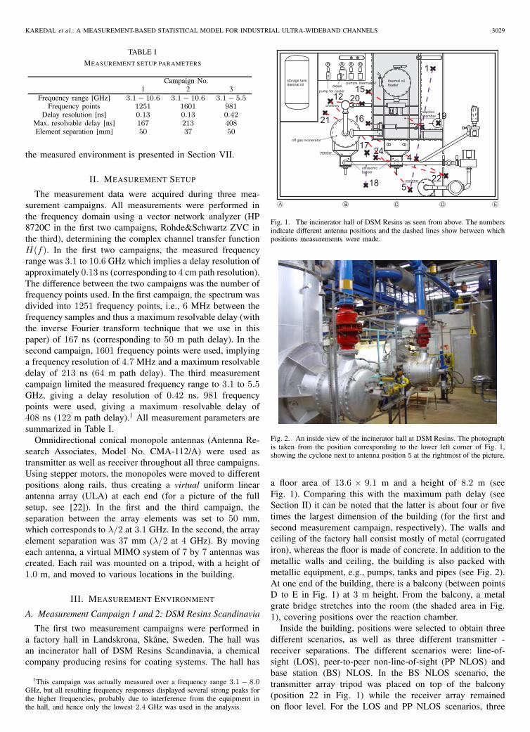
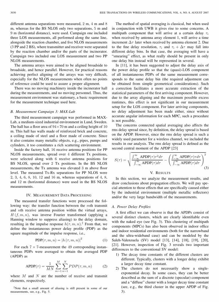
Fig. 1. The incinerator hall of DSM Resins as seen from above. The numbersindicate different antenna positions and the dashed lines show between whichpositions measurements were made.

Fig. 2. An inside view of the incinerator hall at DSM Resins. The photographis taken from the position corresponding to the lower left corner of Fig. 1,showing the cyclone next to antenna position 5 at the rightmost of the picture.

a floor area of 13.6 × 9.1 m and a height of 8.2 m (seeFig. 1). Comparing this with the maximum path delay (seeSection II) it can be noted that the latter is about four or fivetimes the largest dimension of the building (for the first andsecond measurement campaign, respectively). The walls andceiling of the factory hall consist mostly of metal (corrugatediron), whereas the floor is made of concrete. In addition to themetallic walls and ceiling, the building is also packed withmetallic equipment, e.g., pumps, tanks and pipes (see Fig. 2).At one end of the building, there is a balcony (between pointsD to E in Fig. 1) at 3 m height. From the balcony, a metalgrate bridge stretches into the room (the shaded area in Fig.1), covering positions over the reaction chamber.

Inside the building, positions were selected to obtain threedifferent scenarios, as well as three different transmitter -receiver separations. The different scenarios were: line-of-sight (LOS), peer-to-peer non-line-of-sight (PP NLOS) andbase station (BS) NLOS. In the BS NLOS scenario, thetransmitter array tripod was placed on top of the balcony(position 22 in Fig. 1) while the receiver array remainedon floor level. For the LOS and PP NLOS scenarios, three


different antenna separations were measured, 2 m, 4 m and 8m, whereas for the BS NLOS only two separations, 5 m and9 m (horizontal distance), were used. Campaign one includedthree LOS measurements, all performed along the same line,alongside the reaction chamber, and five NLOS measurements(3 PP and 2 BS), where transmitter and receiver were separatedby the reaction chamber and/or the parts of the incinerator.Campaign two included one LOS measurement and two PPNLOS measurements.

The antenna arrays were aimed to be aligned broadside tobroadside, and hence parallel. However, for practical reasonsachieving perfect aligning of the arrays was very difficult,especially for the NLOS measurements when often no pointsof reference could be used to assure a proper alignment.

There was no moving machinery inside the incinerator hallduring the measurements, and no moving personnel. Thus, themeasurement environment was stationary, a basic requirementfor the measurement technique used here.

B. Measurement Campaign 3: MAX-Lab

The third measurement campaign was performed in MAX-Lab, a medium-sized industrial environment in Lund, Sweden.The hall has a floor area of 94×70 m and a ceiling height of 10m. This hall has walls made of reinforced brick and concrete,a ceiling made of steel and a floor made of concrete. Sinceit also contains many metallic objects, e.g., pipes, pumps andcylinders, it too constitutes a rich scattering environment.

Inside the factory hall, 16 receive antenna positions for PPNLOS measurements, spread over 4 different Tx positions,were selected along with 6 receive antenna positions forBS NLOS, spread over 2 Tx positions. In the BS NLOSmeasurements, the Tx antenna was elevated 3 m above floorlevel. The measured Tx-Rx separations for PP NLOS were2, 3, 4, 6, 8, 10, 12 and 16 m, whereas separations of 4, 8,and 12 m (horizontal distance) were used in the BS NLOSmeasurements.

IV. MEASUREMENT DATA PROCESSING

The measured transfer functions were processed the fol-lowing way: the transfer function between the mth transmitand nth receive antenna position within the virtual arrays,H (f, m, n), was inverse Fourier transformed (applying aHanning window to suppress aliasing) to the delay domain,resulting in the impulse response h(τ, m, n).2 From that, wedefine the instantaneous power delay profile (PDP) as thesquare magnitude of the impulse response, i.e.,

PDP(τ, m, n) = |h (τ, m, n)|2 (1)

For each 7 × 7-measurement the 49 corresponding instan-taneous PDPs were averaged to obtain the averaged PDP(APDP) as

APDP(τ) =1

MN

M∑m=1

N∑n=1

PDP (τ, m, n) (2)

where M and N are the number of receive and transmitelements, respectively.

2Note that a small amount of aliasing is still present in some of ourmeasurements, see, e.g., Fig. 5.

The method of spatial averaging is classical, but when usedin conjunction with UWB it gives rise to some concerns. Amultipath component that will arrive at a certain delay τi

when received by antenna array element 1, will arrive a timeincrement Δτ later when received by antenna element 2. Dueto the fine delay resolution, τi and τi + Δτ may fall intodifferent delay bins. In that case, the averaging will have a“smearing” effect, as what really should be present in onlyone delay bin instead will be represented in several.

In [11], it has been suggested to adjust the delay axis ofthe power delay profile so that the (quasi)-LOS componentof all instantaneous PDPs of the same measurement corre-sponds to the same delay bin (the required adjustment canbe obtained from simple geometrical considerations). Sucha correction facilitates a more accurate extraction of thestatistical parameters of the first arriving component. However,due to the array aligning and the maximum possible excessruntimes, this effect is not significant in our measurementsetup for the LOS component. For later arriving components,no delay adjustment has been made either, since withoutaccurate angular information for each MPC, such a procedureis not possible.

The concerns connected spatial averaging also affects therms delay spread since, by definition, the delay spread is basedon the APDP. However, since the rms delay spread is such awidely used parameter for a wireless channel, we included theresults in our analysis. The rms delay spread is defined as thesecond central moment of the APDP [23]

S(τ) =

√√√√∫∞−∞ APDP(τ)τ2dτ∫∞−∞ APDP(τ)dτ

−(∫∞

−∞ APDP(τ)τdτ∫∞−∞ APDP(τ)dτ

)2

(3)V. RESULTS

In this section, we analyze the measurement results, anddraw conclusions about propagation effects. We will pay spe-cial attention to those effects that are specifically caused eitherby the industrial environment (multiple metallic reflectors)and/or the very large bandwidth of the measurements.

A. Power Delay Profiles

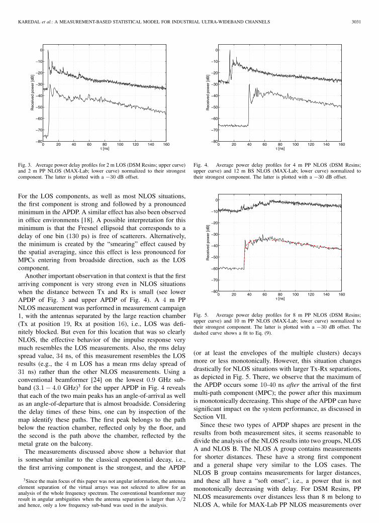
A first effect we can observe is that the APDPs consist ofseveral distinct clusters, which are clearly identifiable evenwith the naked eye (see Fig. 3). This clustering of multipathcomponents (MPCs) has also been observed in indoor officeand indoor residential environments (both for the narrowbandand the ultra-wideband case) and can be modeled by theSaleh-Valenzuela (SV) model [13], [14], [18], [19], [20],[21]. However, inspection of Fig. 3 reveals two importantdifferences to the conventional SV model:

1) The decay time constants of the different clusters aredifferent. Typically, clusters with a longer delay exhibita larger decay time constant.

2) The clusters do not necessarily show a single-exponential decay. In some cases, they can be betterdescribed as the sum of a discrete (specular) componentand a “diffuse” cluster with a longer decay time constant(see, e.g., the third cluster in the upper APDP of Fig.3).


0 20 40 60 80 100 120 140 160−80

−70

−60

−50

−40

−30

−20

−10

0

τ [ns]

Rec

eive

d po

wer

[dB

]

Fig. 3. Average power delay profiles for 2 m LOS (DSM Resins; upper curve)and 2 m PP NLOS (MAX-Lab; lower curve) normalized to their strongestcomponent. The latter is plotted with a −30 dB offset.

For the LOS components, as well as most NLOS situations,the first component is strong and followed by a pronouncedminimum in the APDP. A similar effect has also been observedin office environments [18]. A possible interpretation for thisminimum is that the Fresnel ellipsoid that corresponds to adelay of one bin (130 ps) is free of scatterers. Alternatively,the minimum is created by the “smearing” effect caused bythe spatial averaging, since this effect is less pronounced forMPCs entering from broadside direction, such as the LOScomponent.

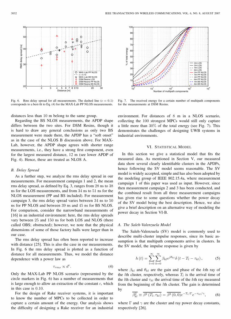
Another important observation in that context is that the firstarriving component is very strong even in NLOS situationswhen the distance between Tx and Rx is small (see lowerAPDP of Fig. 3 and upper APDP of Fig. 4). A 4 m PPNLOS measurement was performed in measurement campaign1, with the antennas separated by the large reaction chamber(Tx at position 19, Rx at position 16), i.e., LOS was defi-nitely blocked. But even for this location that was so clearlyNLOS, the effective behavior of the impulse response verymuch resembles the LOS measurements. Also, the rms delayspread value, 34 ns, of this measurement resembles the LOSresults (e.g., the 4 m LOS has a mean rms delay spread of31 ns) rather than the other NLOS measurements. Using aconventional beamformer [24] on the lowest 0.9 GHz sub-band (3.1 − 4.0 GHz)3 for the upper APDP in Fig. 4 revealsthat each of the two main peaks has an angle-of-arrival as wellas an angle-of-departure that is almost broadside. Consideringthe delay times of these bins, one can by inspection of themap identify these paths. The first peak belongs to the pathbelow the reaction chamber, reflected only by the floor, andthe second is the path above the chamber, reflected by themetal grate on the balcony.

The measurements discussed above show a behavior thatis somewhat similar to the classical exponential decay, i.e.,the first arriving component is the strongest, and the APDP

3Since the main focus of this paper was not angular information, the antennaelement separation of the virtual arrays was not selected to allow for ananalysis of the whole frequency spectrum. The conventional beamformer mayresult in angular ambiguities when the antenna separation is larger than λ/2and hence, only a low frequency sub-band was used in the analysis.

0 20 40 60 80 100 120 140 160−80

−70

−60

−50

−40

−30

−20

−10

0

τ [ns]

Rec

eive

d po

wer

[dB

]

Fig. 4. Average power delay profiles for 4 m PP NLOS (DSM Resins;upper curve) and 12 m BS NLOS (MAX-Lab; lower curve) normalized totheir strongest component. The latter is plotted with a −30 dB offset.

0 20 40 60 80 100 120 140 160−80

−70

−60

−50

−40

−30

−20

−10

0

τ [ns]

Rec

eive

d po

wer

[dB

]

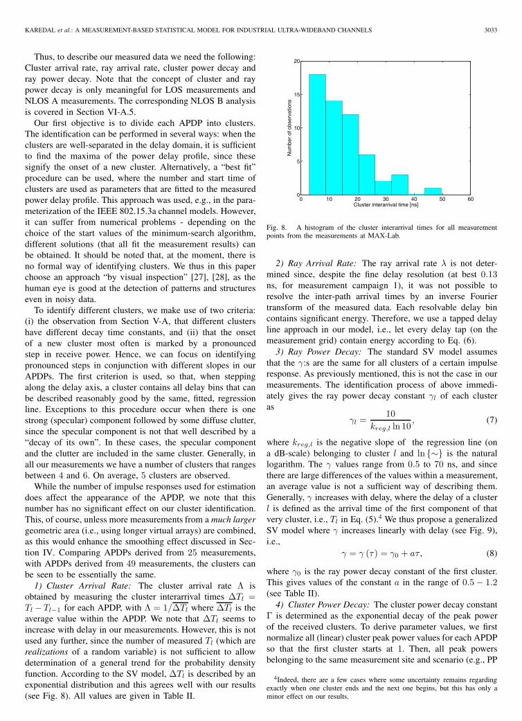
Fig. 5. Average power delay profiles for 8 m PP NLOS (DSM Resins;upper curve) and 10 m PP NLOS (MAX-Lab; lower curve) normalized totheir strongest component. The latter is plotted with a −30 dB offset. Thedashed curve shows a fit to Eq. (9).

(or at least the envelopes of the multiple clusters) decaysmore or less monotonically. However, this situation changesdrastically for NLOS situations with larger Tx-Rx separations,as depicted in Fig. 5. There, we observe that the maximum ofthe APDP occurs some 10-40 ns after the arrival of the firstmulti-path component (MPC); the power after this maximumis monotonically decreasing. This shape of the APDP can havesignificant impact on the system performance, as discussed inSection VII.

Since these two types of APDP shapes are present in theresults from both measurement sites, it seems reasonable todivide the analysis of the NLOS results into two groups, NLOSA and NLOS B. The NLOS A group contains measurementsfor shorter distances. These have a strong first componentand a general shape very similar to the LOS cases. TheNLOS B group contains measurements for larger distances,and these all have a “soft onset”, i.e., a power that is notmonotonically decreasing with delay. For DSM Resins, PPNLOS measurements over distances less than 8 m belong toNLOS A, while for MAX-Lab PP NLOS measurements over


1 2 3 4 5 6 7 8 9 10 20 3020

30

40

50

60

Distance [m]

RM

S d

elay

spr

ead

[ns]

MAX−Lab PP NLOSc = 0.10MAX−Lab BS NLOSDSM Resins LOSDSM Resins PP NLOSDSM Resins BS NLOS

Fig. 6. Rms delay spread for all measurements. The dashed line (c = 0.1)corresponds to a best-fit to Eq. (4) for the MAX-Lab PP NLOS measurements.

distances less than 10 m belong to the same group.Regarding the BS NLOS measurements, the APDP shape

differs between the two sites. For DSM Resins, though itis hard to draw any general conclusions as only two BSmeasurement were made there, the APDP has a “soft onset”as in the case of the NLOS B discussion above. For MAX-Lab, however, the APDP shape agrees with shorter rangemeasurements, i.e., they have a strong first component, evenfor the largest measured distance, 12 m (see lower APDP ofFig. 4). Hence, these are treated as NLOS A.

B. Delay Spread

As a further step, we analyze the rms delay spread in ourmeasurements. For measurement campaign 1 and 2, the meanrms delay spread, as defined by Eq. 3, ranges from 28 ns to 38ns for the LOS measurements, and from 34 ns to 51 ns for theNLOS measurement (PP and BS included). For measurementcampaign 3, the rms delay spread varies between 34 ns to 50ns for PP NLOS and between 39 ns and 45 ns for BS NLOS.For comparison, consider the narrowband measurements of[16] in an industrial environment: here, the rms delay spreadsvary between 25 and 150 ns for both LOS and NLOS (therecalled OBS; obstructed); however, we note that the physicaldimensions of some of those factory halls were larger than inour case.

The rms delay spread has often been reported to increasewith distance [25]. This is also the case in our measurements.In Fig. 6 the rms delay spread is plotted as a function ofdistance for all measurements. Thus, we model the distancedependence with a power law as

τrms ∝ dc. (4)

Only the MAX-Lab PP NLOS scenario (represented by thecircle markers in Fig. 6) has a number of measurements thatis large enough to allow an extraction of the constant c, whichin this case is 0.10.

For the design of Rake receiver systems, it is importantto know the number of MPCs to be collected in order tocapture a certain amount of the energy. Our analysis showsthe difficulty of designing a Rake receiver for an industrial

100

101

102

103

104

0

10

20

30

40

50

60

70

80

90

100

Number of multipath components

% o

f tot

al e

nerg

y

2m LOS2m LOS4m LOS8m LOS2m PP NLOS4m PP NLOS4m PP NLOS8m PP NLOS4m BS NLOS8m BS NLOS

Fig. 7. The received energy for a certain number of multipath componentsfor the measurements at DSM Resins.

environment. For distances of 8 m in a NLOS scenario,collecting the 100 strongest MPCs would still only capturea little more than 30% of the total energy (see Fig. 7). Thisdemonstrates the challenges of designing UWB systems inindustrial environments.

VI. STATISTICAL MODEL

In this section we give a statistical model that fits themeasured data. As mentioned in Section V, our measureddata show several clearly identifiable clusters in the APDPs,hence following the SV model seems reasonable. The SVmodel is widely accepted, simple and has also been adopted bythe modeling group of IEEE 802.15.4a, where measurementcampaign 1 of this paper was used as input. However, sincethen measurement campaign 2 and 3 has been conducted, andthe combined result from all three measurement campaignshas given rise to some questions whether the power decayof the SV model being the best description. Hence, we alsogive a brief description on an alternative way of modeling thepower decay in Section VI-B.

A. The Saleh-Valenzuela Model

The Saleh-Valenzuela (SV) model is commonly used todescribe multi-cluster impulse responses, since its basic as-sumption is that multipath components arrive in clusters. Inthe SV model, the impulse response is given by

h (t) =∞∑

l=0

∞∑k=0

βklejθklδ (t − Tl − τkl) , (5)

where βkl and θkl are the gain and phase of the kth ray ofthe lth cluster, respectively, whereas Tl is the arrival time ofthe lth cluster and τkl the arrival time of the kth ray measuredfrom the beginning of the lth cluster. The gain is determinedby

β2kl ≡ β2 (Tl, τkl) = β2 (0, 0)e−Tl/Γe−τkl/γ , (6)

where Γ and γ are the cluster and ray power decay constants,respectively [26].


Thus, to describe our measured data we need the following:Cluster arrival rate, ray arrival rate, cluster power decay andray power decay. Note that the concept of cluster and raypower decay is only meaningful for LOS measurements andNLOS A measurements. The corresponding NLOS B analysisis covered in Section VI-A.5.

Our first objective is to divide each APDP into clusters.The identification can be performed in several ways: when theclusters are well-separated in the delay domain, it is sufficientto find the maxima of the power delay profile, since thesesignify the onset of a new cluster. Alternatively, a “best fit”procedure can be used, where the number and start time ofclusters are used as parameters that are fitted to the measuredpower delay profile. This approach was used, e.g., in the para-meterization of the IEEE 802.15.3a channel models. However,it can suffer from numerical problems - depending on thechoice of the start values of the minimum-search algorithm,different solutions (that all fit the measurement results) canbe obtained. It should be noted that, at the moment, there isno formal way of identifying clusters. We thus in this paperchoose an approach “by visual inspection” [27], [28], as thehuman eye is good at the detection of patterns and structureseven in noisy data.

To identify different clusters, we make use of two criteria:(i) the observation from Section V-A, that different clustershave different decay time constants, and (ii) that the onsetof a new cluster most often is marked by a pronouncedstep in receive power. Hence, we can focus on identifyingpronounced steps in conjunction with different slopes in ourAPDPs. The first criterion is used, so that, when steppingalong the delay axis, a cluster contains all delay bins that canbe described reasonably good by the same, fitted, regressionline. Exceptions to this procedure occur when there is onestrong (specular) component followed by some diffuse clutter,since the specular component is not that well described by a“decay of its own”. In these cases, the specular componentand the clutter are included in the same cluster. Generally, inall our measurements we have a number of clusters that rangesbetween 4 and 6. On average, 5 clusters are observed.

While the number of impulse responses used for estimationdoes affect the appearance of the APDP, we note that thisnumber has no significant effect on our cluster identification.This, of course, unless more measurements from a much largergeometric area (i.e., using longer virtual arrays) are combined,as this would enhance the smoothing effect discussed in Sec-tion IV. Comparing APDPs derived from 25 measurements,with APDPs derived from 49 measurements, the clusters canbe seen to be essentially the same.

1) Cluster Arrival Rate: The cluster arrival rate Λ isobtained by measuring the cluster interarrival times ΔTl =Tl −Tl−1 for each APDP, with Λ = 1/ΔTl where ΔTl is theaverage value within the APDP. We note that ΔTl seems toincrease with delay in our measurements. However, this is notused any further, since the number of measured Tl (which arerealizations of a random variable) is not sufficient to allowdetermination of a general trend for the probability densityfunction. According to the SV model, ΔTl is described by anexponential distribution and this agrees well with our results(see Fig. 8). All values are given in Table II.

0 10 20 30 40 50 600

5

10

15

20

Cluster interarrival time [ns]

Num

ber

of o

bser

vatio

ns

Fig. 8. A histogram of the cluster interarrival times for all measurementpoints from the measurements at MAX-Lab.

2) Ray Arrival Rate: The ray arrival rate λ is not deter-mined since, despite the fine delay resolution (at best 0.13ns, for measurement campaign 1), it was not possible toresolve the inter-path arrival times by an inverse Fouriertransform of the measured data. Each resolvable delay bincontains significant energy. Therefore, we use a tapped delayline approach in our model, i.e., let every delay tap (on themeasurement grid) contain energy according to Eq. (6).

3) Ray Power Decay: The standard SV model assumesthat the γ:s are the same for all clusters of a certain impulseresponse. As previously mentioned, this is not the case in ourmeasurements. The identification process of above immedi-ately gives the ray power decay constant γl of each clusteras

γl =10

kreg,l ln 10, (7)

where kreg,l is the negative slope of the regression line (ona dB-scale) belonging to cluster l and ln {∼} is the naturallogarithm. The γ values range from 0.5 to 70 ns, and sincethere are large differences of the values within a measurement,an average value is not a sufficient way of describing them.Generally, γ increases with delay, where the delay of a clusterl is defined as the arrival time of the first component of thatvery cluster, i.e., Tl in Eq. (5).4 We thus propose a generalizedSV model where γ increases linearly with delay (see Fig. 9),i.e.,

γ = γ (τ) = γ0 + aτ , (8)

where γ0 is the ray power decay constant of the first cluster.This gives values of the constant a in the range of 0.5 − 1.2(see Table II).

4) Cluster Power Decay: The cluster power decay constantΓ is determined as the exponential decay of the peak powerof the received clusters. To derive parameter values, we firstnormalize all (linear) cluster peak power values for each APDPso that the first cluster starts at 1. Then, all peak powersbelonging to the same measurement site and scenario (e.g., PP

4Indeed, there are a few cases where some uncertainty remains regardingexactly when one cluster ends and the next one begins, but this has only aminor effect on our results.


0 20 40 60 800

20

40

60

80

Cluster delay Tl [ns]

Ray

pow

er d

ecay

con

stan

t γ

[ns]

8m LOS (DSM Resins)a = 1.42m LOS (DSM Resins)a = 0.642m PP NLOS (DSM Resins)a = 1.03

Fig. 9. Example plot of the linear delay dependence of the ray power decayconstant γ. The figure shows γ as a function of delay for three differentmeasurement positions from measurement campaign 1.

TABLE II

SALEH-VALENZUELA MODEL PARAMETERS

DSM 1/Λ Γ γ0 a γ1 γrise χ[ns] [ns] [ns] [ns] [ns]

los 15.83 12.62 3.52 0.80 - - -pp nlos a 13.10 29.78 4.13 1.19 - - -pp nlos b - - - - 66.86 100 0.98

bs nlos (b) - - - - 71.36 11.12 0.90MAX-Labpp nlos a 16.00 28.87 4.98 0.54 - - -pp nlos b - - - - 44.00 14.29 1.00bs nlos (a) 12.53 24.01 2.53 0.69 - - -

NLOS) are plotted on a dB-scale as a function of the excessdelay, and, finally, Γ is determined from a best-fit regressionline in the same way as the ray power decay constant. Thisgives cluster power decay values in the range of 13 − 30 ns(see Table II).

5) PDP Shape for NLOS B: As mentioned in Section V, thepower of the measurements characterized as NLOS B is notmonotonically decreasing, but there is a soft onset starting atthe first arriving MPC where the power is actually increasingwith delay. Hence, the power gains can no longer be describedby Eq. (6). Instead, the power delay dependence is given by

β2kl = Ω1

γ1 + γrise

γ1 (γ1 + γrise (1 − χ))

(1 − χe−τ/γrise

)e−τ/γ1,

(9)where γ1, γrise and χ are shape parameters while Ω1 is thenormalized power [21]. An example plot of the curve fittingof Eq. (9) is shown in Fig. 5. All parameter values are foundin Table II.

B. Alternative Model - Power Law Approach

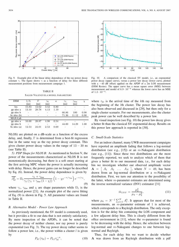
As previously mentioned, the SV model is commonly used,but it provides a fit to our data that is not entirely satisfactory.By mere inspection of the APDPs, it can be noted thatthe power decay of neither cluster, nor ray power is purelyexponential (see Fig. 3). The ray power decay rather seems tofollow a power law, i.e., the power within a cluster l is givenby

Pkl (τkl) = P0,lτ−αkl , (10)

0 20 40 60 80 100 120 140 160−80

−70

−60

−50

−40

−30

−20

−10

0

τ [ns]

Rec

eive

d po

wer

[dB

]

Fig. 10. A comparison of the classical SV model, i.e., an exponentialpower decay (upper curve), versus a power law decay (lower curve, plottedwith a −40 dB offset) applied on the APDP of a 2m LOS measurement(DSM Resins). The upper curve has a mean square error (MSE) betweenmeasurement and model of 6.9 · 10−4 whereas the lower curve has an MSEof 1.2 · 10−4.

where τkl is the arrival time of the kth ray measured fromthe beginning of the lth cluster. The power law decay hasalso been observed and discussed in [29], but then only for asingle-cluster scenario. For our measurements, also the clusterpeak power can be well described by a power law.

By visual inspection (see Fig. 10) the power law decay givesa better fit than the classical SV exponential decay. Results onthis power law approach is reported in [30].

C. Small-Scale Statistics

For an indoor channel, many UWB measurement campaignshave reported an amplitude fading that follows a log-normaldistribution (see e.g., [15]) or an m-Nakagami distribution(see e.g., [11]). Since these two distributions are the mostfrequently reported, we seek to analyze which of them thatgives a better fit to our measured data, i.e., for each delaybin we investigate whether our observed amplitude vectorA =

[A1 A2 . . . AN

], where N = 49, has been

drawn from an log-normal distribution or a m-Nakagamidistribution. First, we turn our attention to the possibility ofthe latter, where m-parameter estimates are determined usingthe inverse normalized variance (INV) estimator [31]

mINV =μ2

2

μ4 − μ22

, (11)

where μk = N−1∑N

i=1 Aki . It appears that for most of the

measurements, an m-parameter estimate of 1 is achieved,which corresponds to a Rayleigh distribution. The only excep-tion is for the delay bin containing the LOS component anda few adjacent delay bins. This is clearly different from theoffice environment in [11], where the m-parameter is foundto be decreasing with the delay. Hence, the selection betweenlog-normal and m-Nakagami changes to one between log-normal and Rayleigh.

Thus, for each delay bin we want to decide whetherA was drawn from an Rayleigh distribution with a pdf


p (A; σR, Rayleigh), where σR is the maximum likelihoodestimate (MLE) of σR given by

σR =

√√√√ 12N

N∑i=1

A2i , (12)

or if A has been drawn from a log-normal distribution witha pdf p (A; μLN , σLN , log-normal), where μLN and σLN arethe MLEs of μ and σ given by the mean and standard deviationof ln {A}, respectively.

To make a choice between the two candidate distributions,we perform a generalized likelihood ratio test (GLRT) thatdecides, without favoring any of the two distributions, aRayleigh distribution being the most likely if

p (A; σR, Rayleigh)p (A; μLN , σLN , log-normal)

> 1. (13)

The result of the GLRT is that a Rayleigh distributionis more probably in more than 80% of the (excess) delaybins for each measurement. Hence, our model assumes thata Rayleigh distribution is applicable at all delays except forthe LOS component. However, in order to avoid having to usedifferent distributions for different delay bins, a more practicalsolution is to apply an m-Nakagami distribution to all delaybins, with an m-value of 1 used for all delay bins except theone containing the LOS component.

Several other tests have also been made in order to verifythe result: (i) a Kolmogorov-Smirnoff test, (ii) a comparisonof the mean square error between on one hand the cdf:s of aRayleigh distribution and the measured data, and on the otherthe cdf:s a log-normal distribution and the measured data, (iii)a comparison of the Kullback-Leibler (KL) distance betweena Rayleigh distribution and the measured data versus the KLdistance between a log-normal distribution and the measureddata. All of these tests have a few weaknesses, but regardlessof these, all tests point towards a Rayleigh distribution.

The Rayleigh fading amplitude is a somewhat surprisingresult since it has been assumed that the fine resolutionof the UWB would imply a too small number of pathsarriving in each delay bin to fulfil the central limit theorem(CLT). A possible explanation why Rayleigh fading is yetobserved here is that the high density of scatterers of theindustrial environment creates a number of paths that is highenough to fulfil the CLT. An alternative explanation is that theproblems of spatial averaging described in Section IV causesthe Rayleigh distribution, i.e., the 49 values constituting thestatistical ensemble for a certain delay bin may not be samplesof the same MPC, but instead samples of several differentMPCs.

D. Pathloss

The distance dependent pathloss is determined from scatterplots of the received power and modeled in dB, as

PL (d) = PL0 + 10n log10

(d

d0

)+ Xσ (14)

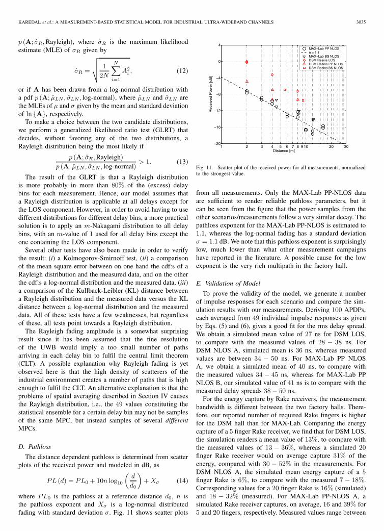
where PL0 is the pathloss at a reference distance d0, n isthe pathloss exponent and Xσ is a log-normal distributedfading with standard deviation σ. Fig. 11 shows scatter plots

1 2 3 4 5 6 7 8 9 10 20 30−20

−16

−12

−8

−4

0

4

Distance [m]

Rec

eive

d P

ower

[dB

]

MAX−Lab PP NLOSn = 1.1MAX−Lab BS NLOSDSM Resins LOSDSM Resins PP NLOSDSM Resins BS NLOS

Fig. 11. Scatter plot of the received power for all measurements, normalizedto the strongest value.

from all measurements. Only the MAX-Lab PP-NLOS dataare sufficient to render reliable pathloss parameters, but itcan be seen from the figure that the power samples from theother scenarios/measurements follow a very similar decay. Thepathloss exponent for the MAX-Lab PP-NLOS is estimated to1.1, whereas the log-normal fading has a standard deviationσ = 1.1 dB. We note that this pathloss exponent is surprisinglylow, much lower than what other measurement campaignshave reported in the literature. A possible cause for the lowexponent is the very rich multipath in the factory hall.

E. Validation of Model

To prove the validity of the model, we generate a numberof impulse responses for each scenario and compare the sim-ulation results with our measurements. Deriving 100 APDPs,each averaged from 49 individual impulse responses as givenby Eqs. (5) and (6), gives a good fit for the rms delay spread.We obtain a simulated mean value of 27 ns for DSM LOS,to compare with the measured values of 28 − 38 ns. ForDSM NLOS A, simulated mean is 36 ns, whereas measuredvalues are between 34 − 50 ns. For MAX-Lab PP NLOSA, we obtain a simulated mean of 40 ns, to compare withthe measured values 34 − 45 ns, whereas for MAX-Lab PPNLOS B, our simulated value of 41 ns is to compare with themeasured delay spreads 38 − 50 ns.

For the energy capture by Rake receivers, the measurementbandwidth is different between the two factory halls. There-fore, our reported number of required Rake fingers is higherfor the DSM hall than for MAX-Lab. Comparing the energycapture of a 5 finger Rake receiver, we find that for DSM LOS,the simulation renders a mean value of 13%, to compare withthe measured values of 13 − 36%, whereas a simulated 20finger Rake receiver would on average capture 31% of theenergy, compared with 30 − 52% in the measurements. ForDSM NLOS A, the simulated mean energy capture of a 5finger Rake is 6%, to compare with the measured 7 − 18%.Corresponding values for a 20 finger Rake is 16% (simulated)and 18 − 32% (measured). For MAX-Lab PP-NLOS A, asimulated Rake receiver captures, on average, 16 and 39% for5 and 20 fingers, respectively. Measured values range between


14 and 33% for a 5 finger Rake, and between 34 and 59%for a 20 finger Rake. Finally, for MAX-Lab PP-NLOS B, thesimulated mean energy capture for a 5 and 20 finger Rake,respectively, is 10 and 29%, to compare with the measuredvalues 12 − 17% and 31 − 40%.

VII. SUMMARY AND CONCLUSIONS

We presented measurements of the ultra-wideband channelin two factory halls. The measurements cover a bandwidthfrom 3.1−10.6 or 3.1−5.5 GHz, and thus give very fine delayresolution. The main results can be summarized as follows:

• Due to the presence of multiple metallic reflectors, themultipath environments are dense; in other words, almostall resolvable delay bins contain significant energy -especially for NLOS situations at larger distances. Thisis in contrast to UWB office environments, as described,e.g., in [15].

• The inter-path arrival times were so small that they werenot resolvable even with a delay resolution of 0.13 ns.

• For shorter distances, a strong first component exists,irrespective of whether there is LOS or not.

• For larger distances and PP NLOS scenarios, the max-imum of the power delay profile is several tens ofnanoseconds after the arrival of the first component. Thecommon approximation of a single-exponential PDP doesnot hold at all in those cases.

• Clusters of MPCs can be observed.• Delay spreads range from 30 ns for LOS scenarios at

shorter distances to 50 ns for NLOS at larger distances.

We have also established a statistical model that describesthe behavior of the channel, where it is found that the powerdelay profile can be well described by a generalized Saleh-Valenzuela model (with model parameters given in Table II),which is also used in the IEEE 802.15.4a channel models [21].There are several noteworthy points:

• In contrast to the classical SV model, the ray power decayconstants depend on the excess delay. This dependenceis well described by a linear relationship. The decayconstants vary between 0.5 and 70 ns.

• The peak cluster power can be described by an exponen-tial function of the excess delay.

• The number of clusters varies between 4 and 6.• The small-scale fading is well described by a Rayleigh

distribution, except for the first components in eachcluster, which can show a strong specular contribution.

Additionally, we found that the number of MPCs that isrequired for capturing 50% of the energy of the impulseresponse can be very high, up to 200. This serves as motivationto investigate suboptimum receiver structures that do notrequire one correlator per MPC, e.g., transmitted-referenceschemes, [32], [33], [34], as well as noncoherent schemes.Also, the energy capture of partial Rake receivers, that matchtheir fingers to the first arriving multipath components, will behighly affected in our measured NLOS scenarios, especially atlarger distances.5 This is due to the fact that the maximum of

5The overall performance, however, is determined by the combination ofpathloss, amount of fading, and energy capture.

the PDP occurs some 250 taps after the arrival of the firstMPC. Furthermore, the pronounced minimum between theLOS component and the subsequent components also reducesthe energy capture of the partial Rake in LOS scenarios. Wealso find that a considerable percentage of the received energylies outside a 60 ns wide window; this is important in thecontext of a current IEEE 802.15.3a standardization proposal,which uses OFDM with a 60 ns guard interval.

Our results emphasize the crucial importance of realisticchannel models for system design. Parts of the measurementshave been used as an input to the IEEE 802.15.4a channelmodeling group, which (among other issues) recently havedeveloped a channel model for industrial environments. Ourmeasurement results thus allow a better understanding ofUWB factory channels, and provide guidelines for robustsystem design in such environments.

VIII. ACKNOWLEDGEMENTS

We thank DSM Resins Scandinavia for their permission toperform the measurements in their factory hall. Especially, wewould like to thank Mr. Bengt-Ake Ling, Mr. Gert Wranning,and Mr. Alf Jonsson for their help and cooperation. We wouldalso like to express gratitude to MAX-Lab for their permissionto letting us perform measurements and to Mr. M. GufranKhan and Mr. Asim A. Ashraf for their assistance duringmeasurement campaign 3. Part of this work was financiallysupported by an INGVAR grant of the Swedish StrategicResearch Foundation and the SSF Center for High SpeedWireless Communication.

REFERENCES

[1] R. A. Scholtz, “Multiple access with time-hopping impulse modulation,”in Proc. IEEE Military Communications Conference, vol. 2, 1993, pp.447–450.

[2] M. Z. Win and R. A. Scholtz, “Ultra-wide bandwidth time-hoppingspread-spectrum impulse radio for wireless multiple-access communi-cations,” IEEE Trans. Commun., vol. 48, pp. 679–691, Apr. 2000.

[3] C. J. LeMartret and G. B. Giannakis, “All-digital PAM impulse radio formultiple-access through frequency-selective multipath,” in Proc. IEEEGlobal Telecommunications Conference, 2000, pp. 77–81.

[4] M. G. diBenedetto, T. Kaiser, A. F. Molisch, I. Oppermann, C. Politano,and D. Porcino (eds.), UWB communications systems, a comprehensiveoverview. Hindawi Publishing, 2005.

[5] Federal Communications Commission, “First report and order 02-48,”2002.

[6] M. Z. Win and R. A. Scholtz, “Impulse radio: how it works,” IEEECommun. Lett., vol. 2, pp. 36–38, Feb. 1998.

[7] ——, “On the robustness of ultra-wide bandwidth signals in densemultipath environments,” IEEE Commun. Lett., vol. 2, no. 2, pp. 51–53,Feb. 1998.

[8] ——, “On the energy capture of ultra-wide bandwidth signals in densemultipath environments,” IEEE Commun. Lett., vol. 2, no. 9, pp. 245–247, Sept. 1998.

[9] C. Duan, G. Pekhteryev, J. Fang, Y. Nakache, J. Zhang, K. Tajima,Y. Nishioka, and H. Hirai, “Transmitting multiple HD video streams overUWB links,” in Proc. IEEE Consumer Communications and NetworkingConference, vol. 2, Jan. 2006, pp. 691–695.

[10] A. F. Molisch, Wireless Communications. Chichester, West Sussex,UK: IEEE Press–Wiley, 2005.

[11] D. Cassioli, M. Z. Win, and A. F. Molisch, “The ultra-wide bandwidthindoor channel: From statistical models to simulations,” IEEE J. Sel.Areas Commun., vol. 20, no. 6, pp. 1247–1257, Aug. 2002.

[12] S. Ghassemzadeh, R. Jana, C. Rice, W. Turin, and V. Tarokh, “Measure-ment and modeling of an ultra-wide bandwidth indoor channel,” IEEETrans. Commun., vol. 52, pp. 1786–1796, 2004.

[13] C.-C. Chong and S. K. Yong, “A generic statistical based UWB channelmodel for highrise apartments,” IEEE Trans. Antennas Propag., vol. 53,no. 8, pp. 2389–2399, Aug. 2005.


[14] C.-C. Chong, Y. Kim, S. K. Yong, and S. S. Lee, “Statistical char-acterization of the UWB propagation channel in indoor residentialenvironment,” Wiley J. Wireless Commun. Mobile Computing, vol. 5,no. 5, pp. 503–512, Aug. 2005.

[15] A. F. Molisch, J. R. Foerster, and M. Pendergrass, “Channel models forultrawideband personal area networks,” IEEE Personal Commun. Mag.,vol. 10, pp. 14–21, Dec. 2003.

[16] T. S. Rappaport, S. Y. Seidel, and K. Takamizawa, “Statistical channelimpulse response models for factory and open plan building radiocommunication system design,” IEEE Trans. Commun., vol. 39, no. 5,pp. 794–807, May 1991.

[17] R. C. Qiu, “A generalized time domain multipath channel and itsapplication in ultra-wideband UWB wireless optimal receiver design -Part II: Physics-based system analysis,” IEEE Trans. Wireless Commun.,vol. 3, no. 6, pp. 2312–2324, 2004.

[18] J. Kunisch and J. Pamp, “Measurement results and modeling aspectsfor the UWB radio channel,” in IEEE Conference on Ultra WidebandSystems and Technologies Digest of Technical Papers, 2002, pp. 19–23.

[19] A. S. Y. Poon and M. Ho, “Indoor multiple-antenna channel characteri-zation from 2 to 8 GHz,” in Proc. Int. Conference on Communications,May 2003.

[20] A. F. Molisch, “Ultrawideband propagation channels - theory, measure-ment, and modeling,” IEEE Trans. Veh. Technol., vol. 54, no. 5, pp.1528–1545, Sept. 2005.

[21] A. F. Molisch et al., “IEEE 802.15.4a channel model - final report, Tech.Rep. Document IEEE 802.15-04-0662-02-004a, 2005.

[22] J. Karedal, F. Tufvesson, P. Almers, S. Wyne, and A. F. Molisch, “Setupfor frequency domain ultra-wideband measurements using the virtualarray principle,” Dept. of Electroscience, Lund University, Sweden,Tech. Rep. ISSN 1402-8840, No. 9, Sep. 2006.

[23] T. S. Rappaport, Wireless Communications—Principles and Practices.Upper Saddle River, NJ: Prentice Hall, 1996.

[24] H. Krim and M. Viberg, “Two decades of array signal processing: Theparametric approach,” IEEE Signal Processing Mag., vol. 13, no. 4, pp.67–94, July 1996.

[25] L. J. Greenstein, V. Erceg, Y. S. Yeh, and M. V. Clark, “A new path-gain/delay-spread propagation model for digital cellular channels,” IEEETrans. Veh. Technol., vol. 46, no. 2, pp. 477–485, May 1997.

[26] A. A. M. Saleh and R. A. Valenzuela, “A statistical model for indoormultipath propagation,” IEEE J. Sel. Areas Commun., vol. 5, no. 2, pp.128–137, Feb. 1987.

[27] L. Vuokko, P. Vainikainen, and J. Takada, “Clusters extracted frommeasured propagation channels in macrocellular environments,” IEEETrans. Antennas Propag., vol. 53, pp. 4089–4098, Dec. 2005.

[28] M. Toeltsch, J. Laurila, K. Kalliola, A. F. Molisch, P. Vainikainen, andE. Bonek, “Statistical characterization of urban spatial radio channels,”IEEE J. Sel. Areas Commun., vol. 20, pp. 539–549, Apr. 2002.

[29] J. B. Andersen and P. Eggers, “A heuristic model of power delay profilesin landmobile communications,” in Proc. URSI International Symposiumon Electromagnetic Theory, Sydney, 1992, pp. 55–57.

[30] J. Karedal, F. Tufvesson, and A. F. Molisch, IEEE Commun. Lett., tobe published.

[31] A. Abdi and M. Kaveh, “Performance comparison of three different es-timators for the Nakagami m parameter using Monte Carlo simulation,”IEEE Commun. Lett., vol. 4, no. 4, pp. 119–121, Apr. 2000.

[32] J. D. Choi and W. E. Stark, “Performance of ultra-wideband communi-cations with suboptimal receivers in multipath channels,” IEEE J. Sel.Areas Commun., vol. 20, no. 9, pp. 1754–1766, Dec. 2002.

[33] F. Tufvesson, S. Gezici, and A. F. Molisch, “Ultra-wideband communi-cations using hybrid matched filter correlation receivers,” IEEE Trans.Wireless Commun., in press.

[34] T. Q. S. Quek and M. Z. Win, “Analysis of UWB transmitted referencecommunication systems in dense multipath channels,” IEEE J. Sel. AreasCommun., vol. 23, no. 9, pp. 1863–1874, Sept. 2005.

Johan Karedal received the M.S. degree in engi-neering physics in 2002 from Lund University inSweden. In 2003, he started working towards thePh.D. degree at the Department of Electroscience,Lund University, where his research interests are onchannel measurement and modeling for MIMO andUWB systems. He has participated in the Europeanresearch initiative “MAGNET.”

Shurjeel Wyne received his B.Sc. degree in elec-trical engineering from UET Lahore in Pakistan,and his M.S. degree in digital communications fromChalmers University of Technology, Gothenburg inSweden. In 2003, he joined the radio systems groupat Lund University in Sweden, where he is workingtowards his PhD. His research interests are in thefield of measurement and modeling of wireless prop-agation channels particularly for MIMO systems.Shurjeel has participated in the European researchinitiative “COST273,” and is currently involved in

the European network of excellence “NEWCOM.”

Peter Almers received the M.S. degree in elec-trical engineering in 1998 from Lund Universityin Sweden. In 1998, he joined the radio researchdepartment at TeliaSonera AB (formerly Telia AB),in Malmo, Sweden, mainly working with WCDMAand 3GPP standardization physical layer issues. Pe-ter is currently working towards the Ph.D. degree atthe Department of Electroscience, Lund University.He has participated in the European research initia-tives “COST273,” and is currently involved in theEuropean network of excellence “NEWCOM” and

the NORDITE project “WILATI.” Peter received an IEEE Best Student PaperAward at PIMRC in 2002.

Fredrik Tufvesson was born in Lund, Sweden in1970. He received the M.S. degree in ElectricalEngineering in 1994, the Licentiate Degree in 1998and his Ph.D. in 2000, all from Lund Universityin Sweden. After almost two years at a startupcompany, Fiberless Society, Fredrik is now associateprofessor at the department of Electroscience. Hismain research interests are channel measurementsand modeling for wireless communication, includ-ing channels for both MIMO and UWB systems.Beside this, he also works with channel estimation

and synchronization problems, OFDM system design and UWB transceiverdesign.

Andreas F. Molisch (S’89, M’95, SM’00, F’05)received the Dipl. Ing., Dr. techn., and habilitationdegrees from the Technical University Vienna (Aus-tria) in 1990, 1994, and 1999, respectively. From1991 to 2000, he was with the TU Vienna, becomingan associate professor there in 1999. From 2000-2002, he was with the Wireless Systems ResearchDepartment at AT&T (Bell) Laboratories Researchin Middletown, NJ. Since then, he has been withMitsubishi Electric Research Labs, Cambridge, MA,USA, where he is now Distinguished Member of

Technical Staff. He is also professor and chairholder for radio systems atLund University, Sweden.

Dr. Molisch has done research in the areas of SAW filters, radiative transferin atomic vapors, atomic line filters, smart antennas, and wideband systems.His current research interests are measurement and modeling of mobileradio channels, UWB, cooperative communications, and MIMO systems.Dr. Molisch has authored, co-authored or edited four books, among themthe recent textbook Wireless Communications (Wiley-IEEE Press), 11 bookchapters, some 100 journal papers, and numerous conference contributions.

Dr. Molisch is an editor of the IEEE Transactios Wireless Communications,co-editor of recent and upcoming special issues on UWB (in IEEE Journalon Selected Areas in Communications and Proc. IEEE). He has been memberof numerous TPCs, vice chair of the TPC of VTC 2005 spring, general chairof ICUWB 2006, and TPC co-chair of the wireless symposium of Globecom2007. He has participated in the European research initiatives “COST 231,”“COST 259,” and “COST273,” where he was chairman of the MIMO channelworking group, he was chairman of the IEEE 802.15.4a channel modelstandardization group, and is also chairman of Commission C (signals andsystems) of URSI (International Union of Radio Scientists). Dr. Molisch is aFellow of the IEEE, an IEEE Distinguished Lecturer, and recipient of severalawards.

A Measurement-Based Statistical Model for Industrial Ultra-Wideband Channels

Documents