A Maze Solver for Android - Stanford University · A Maze Solver for Android Rohan Paranjpe Department of Electrical Engineering Stanford University Stanford, CA 94305 Email: [email protected]

A Maze Solver for AndroidRohan Paranjpe

Department of Electrical EngineeringStanford UniversityStanford, CA 94305

Email: [email protected]

Armon SaiedDepartment of Electrical Engineering

Stanford UniversityStanford, CA 94305

Email: [email protected]

Abstract—Solving mazes and extracting shortest path solutionshave a number of applications within image processing. Inthis paper, we provide an algorithm and develop an Androidapplication used to detect and solve rectangular mazes usingregion labeling, morphological thinning, and template matching.We provide a detailed analysis for our app’s performance in fourcategories of simply connected mazes and achieve a high successrate with canonical mazes, those whose walls are approximatelyas thick as their path space. We provide a discussion on someinteresting applications of our algorithm and shortest pathproblems within image processing, and improvements upon thealgorithm to increase its robustness and success rate.

I. INTRODUCTION AND MOTIVATION

We encounter many different kinds of puzzles everydayand often need the shortest path between two points or asolution. Our motivation behind this project was to createan application which can automatically solve a maze forthe user. Maze solving and shortest path algorithms withinimage processing are very important in a number of differentapplications ranging from route mapping to feature extractionand seam carving within images [1]. In this paper, we presentan image processing application which obtains an image of amaze, extracts the solution space, solves the maze, and thenoverlays the solution over the original image.

Mazes in general are extremely varied in terms of com-plexity, topology, and shape, so we first need to restrict ourspace of mazes to those which are simply-connected, meaningthere are only two disjoint walls in our maze, and those whichhave their starts and ends on their edge. Note that within thisdefinition we do not require a strictly rectangular maze, butthat for the most part, rectangularly shaped mazes will be ourprimary type of maze by default. We use these restrictions tolimit our mazes to those with no loops, and those whose startsand ends are detectable via image processing.

Our goal was to create a mobile application which doesall processing on the phone (no server-side communication),and that can detect unusual-looking mazes, but only thosethat follow our criteria above (e.g. hand-drawn mazes, oraerial views of hedge mazes). We used the Android mobileplatform and OpenCV toolbox for common image processingfunctions ranging from adaptive thresholding and erosion tomore complicated morphological operations such as regionlabeling and convex hull calculations.

The paper is organized as follows. Part II will coverAlgorithm Development, including justification of our steps

and processes. Part III will cover our results and observationswith different test cases. Part IV will include our conclusions,further improvements, and relevance within image processing.

II. ALGORITHM DEVELOPMENT

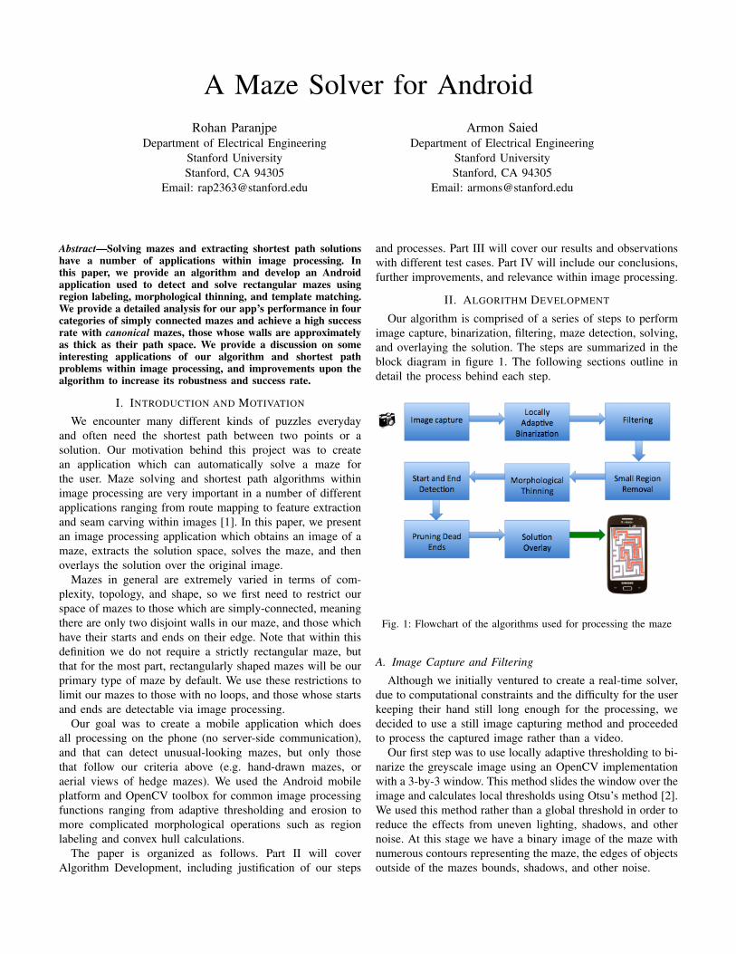
Our algorithm is comprised of a series of steps to performimage capture, binarization, filtering, maze detection, solving,and overlaying the solution. The steps are summarized in theblock diagram in figure 1. The following sections outline indetail the process behind each step.

Fig. 1: Flowchart of the algorithms used for processing the maze

A. Image Capture and Filtering

Although we initially ventured to create a real-time solver,due to computational constraints and the difficulty for the userkeeping their hand still long enough for the processing, wedecided to use a still image capturing method and proceededto process the captured image rather than a video.

Our first step was to use locally adaptive thresholding to bi-narize the greyscale image using an OpenCV implementationwith a 3-by-3 window. This method slides the window over theimage and calculates local thresholds using Otsu’s method [2].We used this method rather than a global threshold in order toreduce the effects from uneven lighting, shadows, and othernoise. At this stage we have a binary image of the maze withnumerous contours representing the maze, the edges of objectsoutside of the mazes bounds, shadows, and other noise.

For small noise reduction at this point, we applied a 3-by-3median filter. This worked for small effects such as salt-and-pepper noise or random fluctuations in the image. Our nextstep was to detect the maze itself by region labeling withinthe image. We used a region labeling function in OpenCV tolabel the various connected regions within our black and whiteimage. Given our restriction of the maze space, we knew thatour maze would consist of two walls. Our next assumption liedwithin the idea that the maze walls, while perhaps thin andsmall in area compared to other objects in the image, wouldcertainly have large perimeters. And so we identified the tworegions with the largest perimeters as the walls of the maze,and set the remaining regions to the background.

At this point in the process our image was nearly noise-free,and comprised of the maze walls in black, with the rest of theimage in white. Our next step was to filter out everythingbut the maze, and only operate on the solution path. Initially,we tried using a binary mask built from the convex hull ofthe maze walls, but this was not robust to slight rotations orgeometric shrinking/dilation of the maze image. As a result,the convex hull of the regions would leave strips of whitealong the edge of the maze walls which could later contributeto a bad start/end detection scheme.

To rectify this, we used a slightly different method to extracta better binary mask, which would include only the maze wallsand the solution space. In order to correctly extract this mask,we needed to mathematically define points which fit thesecriteria.

With two maze walls, we are essentially trying to findthe set of all convex combinations between these two walls.Mathematically, let W1 be the set of all (x, y) points withinthe first wall, and let W2 be the set of all points within thesecond. Define the set A as:

A = {(x, y)|(x, y) = λ(x1, y1) + (1− λ)(x2, y2),(x1, y1) ∈W1, (x2, y2) ∈W2, 0 ≤ λ ≤ 1}

Calculation of A required a bit more computation, but ensureda binary mask free from sliver artifacts. After applying themask, as a final filter, we used region labeling to extract smallregions, so that by the end of our preprocessing, we were leftonly with a binary image, with the solution path in white, andthe background in black.

B. Morphological Thinning of the Solution SpaceOur next step was to use morphological thinning to obtain

a full skeletal path of the solution space. This was importantfor a number of reasons: to simplify our solution search, toprune the non-solution path, and to simplify obtaining the finalsolution from the path space. But in order to obtain a usableskeleton, we required a thinning process that would leave uswith the following features:• one-pixel wide• completely connected• no loopsThe one-pixel width requirement is for facilitating our

pruning process (pixelating the wrong paths). There are lots of

quick thinning algorithms that do not guarantee that a regiongives a connected skeleton. In the scope of our project, if aparticular path was to have a gap within the skeleton, thiswould mean we could never extract a solution that wouldrun through that path. After trying out various algorithms,we finally used the Zhang-Suen thinning algorithm, whichguarantees connectivity and a one-pixel wide solution [3].Unfortunately, even this algorithm does not completely satisfyall of our requirements for a proper pruning algorithm, and ourfurther developments will be elaborated on in the “Pruning andSolution Overlay” section.

Once we obtained a workable skeleton, we had to classifyparticular pixels within the maze as members of the followingsets: endpoints, junctions, and path pixels. Endpoints are pixelswith only one neighboring white pixel, junctions are pixelswith strictly more than two white neighbors, and path pixelsare pixels with only two neighboring white pixels. We used8-connectivity to measure the number of neighbors for aparticular pixel (this includes diagonal as well as horizontaland vertical neighbors). The starts and ends of the maze arealso deadends, and so start/end detection can be classified asa problem where we need to find the most likely two pointswithin our set of endpoints that are the start and end of themaze.

C. Start and End DetectionDetecting the start and end of the maze was a somewhat

difficult task in practice. We developed several algorithms todetect the start and end points of the maze, all of varying effec-tiveness. Our final implementation comprised of the followingsteps:

1) Using a binary mask to acquire the outermost regionsof the maze

2) Using a ranking function on each endpoint to determineits likelihood of being the start or end.

3) Extracting the two highest value endpoints according tothe ranking

To determine the regions of the start and end points we usedthe fact that the entrance and exit to the maze lie on the maze’sedge. By creating a bounding box of the maze walls we wereable to acquire a minimum-bounding rectangle with a borderof some variable width. We determined this width empirically;a width that’s too small for the mask would not pick up manypixels, but a width too large might pick up pixels that arenot in the start and end regions, but within the maze itself.After determining an appropriately sized mask, we obtained abinary image with a large number of pixels in the start andend regions, and a smaller number of pixels in other regions.We define a set W which contains all white pixels after thisoperation.

Obviously, the start and end of the maze will lie close toor within the regions with a large number of pixels. In orderto determine an endpoint’s likelihood of being a start or end,we used the following ranking function:

f(i) =∑j∈W

e−rij/r0

(a) I=0 (b) I=1 (c) I=2

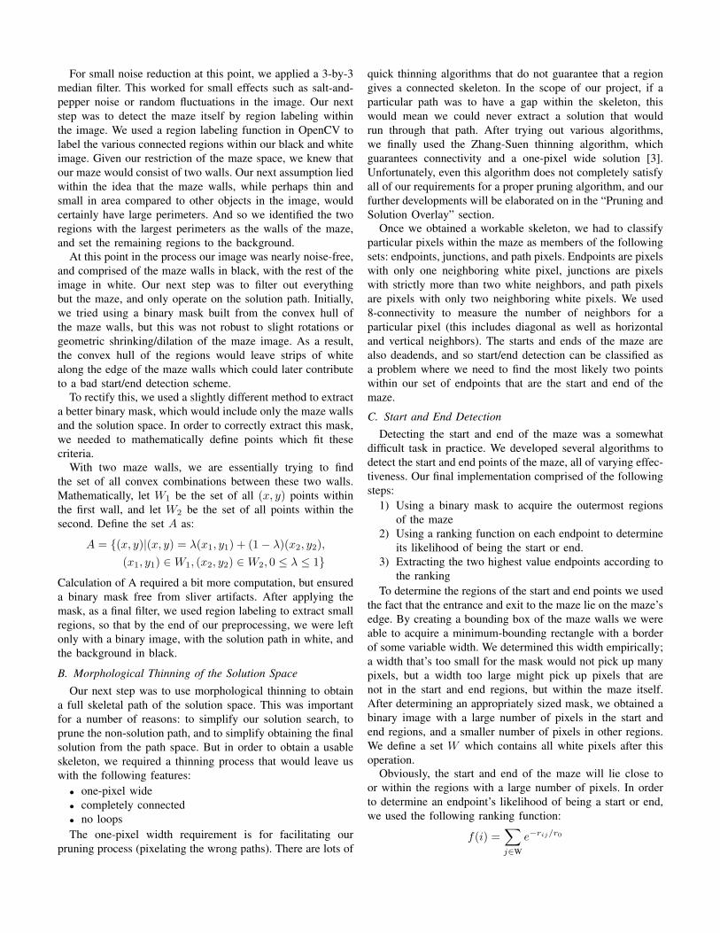
Fig. 2: Shown above is the maze in graph form with S,D,E,and Jrepresenting the start, dead ends, end, and junctions of the maze.Each graph shows a successive iteration with the algorithm until weare left only with a solution path from the start to the end. I representsthe number of iterations that have taken place.

where rij is the Euclidean distance between an endpoint i andone of the white pixels j, and r0 is a scaling factor for theexponential. We can see that an endpoint located very closeto a cluster of white pixels will obtain a high value, and onefarther away obtains much less weight. This works very wellfor separated start and end points, and helps eliminate incorrectendpoints. There are however, some faults to this method.One is that if the skeleton produces two endpoints that arein the start or end region (which can happen as a result ofthe thinning algorithm), we may classify both of these as thestart and end of the maze (which would result in a very sillylooking solution). There are ways to fix this: one could invokeclustering to try and select one representative endpoint from aregion, and one from the other, but for most of our solutions,this sum of exponentials ranking worked fine (even in caseswhere the start and end were located next to each other in themaze).

The final step simply took the highest valued endpoints andextracted them from the list of endpoints.

D. Pruning and Solution Overlay

Our final post-processing step was to iteratively pruneendpoints from the skeleton until we were left with an un-changing skeletal path. Mathematically, this lies on a graphicalassumption about the maze, namely that endpoints will neverbe connected to other endpoints, and will only be connectedto junctions. Figure 2 shows graphs of junctions, endpoints,start and ends and the iterative process taking place. If we startpixelating by starting from the endpoints, we can iterativelyremove parts that are not part of the solution space (reclassify-ing junctions that lose their neighbors as endpoints during theprocess), until no more endpoints exist. This non-recursive im-plementation was important for producing the desired resultsquickly and without requiring too much memory.

Unfortunately, there are particular skeletons that are unsolv-able for our pruning algorithm. Specifically, if the skeletonproduced contains two or three connected junctions, it cannotbe pruned correctly. As an example, L-junctions or T-junctionscan produce unpruneable structures. This is why, in addition toZhang-Suen thinning, we had to employ a template matchingfilter to extract L and T junctions from the maze as well. Ourfinal post-processing steps were to take the pruned skeletalimage, use dilation in order to thicken the solution, and overlayit in red over the original color image.

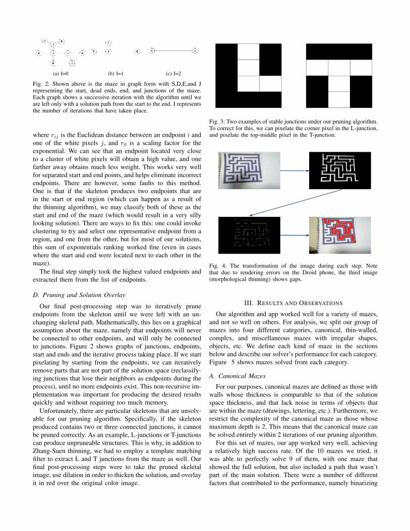
Fig. 3: Two examples of stable junctions under our pruning algorithm.To correct for this, we can pixelate the corner pixel in the L-junction,and pixelate the top-middle pixel in the T-junction.

Fig. 4: The transformation of the image during each step. Notethat due to rendering errors on the Droid phone, the third image(morphological thinning) shows gaps.

III. RESULTS AND OBSERVATIONS

Our algorithm and app worked well for a variety of mazes,and not so well on others. For analysis, we split our group ofmazes into four different categories, canonical, thin-walled,complex, and miscellaneous mazes with irregular shapes,objects, etc. We define each kind of maze in the sectionsbelow and describe our solver’s performance for each category.Figure 5 shows mazes solved from each category.

A. Canonical Mazes

For our purposes, canonical mazes are defined as those withwalls whose thickness is comparable to that of the solutionspace thickness, and that lack noise in terms of objects thatare within the maze (drawings, lettering, etc.). Furthermore, werestrict the complexity of the canonical maze as those whosemaximum depth is 2. This means that the canonical maze canbe solved entirely within 2 iterations of our pruning algorithm.

For this set of mazes, our app worked very well, achievinga relatively high success rate. Of the 10 mazes we tried, itwas able to perfectly solve 9 of them, with one maze thatshowed the full solution, but also included a path that wasn’tpart of the main solution. There were a number of differentfactors that contributed to the performance, namely binarizing

Fig. 5: Shown above are four mazes from each of our definedcategories. The top-left, top-right, bottom-left, and bottom-right showour application’s solution for a canonical maze, a complex maze,a thin maze solved, and a maze from the miscellaneous categoryrespectively.

the maze and detecting the start and end correctly. With thealgorithms we implemented, canonical mazes were generallysolved pretty easily and errors were usually within the actualsolving algorithm or were correlated with a grouping of twoor more connected junctions.

B. Complex Mazes

Complex mazes are similar to the canonical maze, exceptthat their maximum depth is strictly greater than 2. Froman image processing standpoint these mazes are of the samedifficulty as the canonical maze. However, because of theirdepth, a lot more pruning needs to take place before thesolution can be shown. Because of this, there is a higherprobability of error and looped junctions, and so the app doesnot always solve complex mazes. Often, we found that changeslike the orientation of the maze (by 90 degree rotations) couldalter the final solution. We attribute this error to the occasionalintroduction of loops due to the Zhang-Suen algorithm notpreserving homotopy [4].

There are methods to fix this as well, and we will expandupon some of these ideas in the conclusion. For the most part,we were able to obtain full solutions for most complex mazes(although not on the first try at all times). Usually we obtainedeither partial or full solutions with extended non-solution pathsfor this category of mazes.

C. Thin-walled Mazes

We define thin-walled mazes as those that have walls ofthickness significantly smaller than the width of the pathspace. We chose this category to demonstrate the limitationsof our algorithm. Thin-walled mazes can present problems forprimarily two aspects of our implementation.

First, recall that our method of start and end point detectiondefines a bounding box of the maze space and uses a heuristicof shrinking the box dimensions by a predefined number ofpixels. This process pinpoints the entrance and exit of the maze

Fig. 6: This is a maze that was solved, but still retains non-solutionpaths in the structure. We classify this as a “partially solved” maze.

since the edges of the masked image will be black uniformlyexcept at the desired locations. Given the constraints of thismethod, our application struggles to define the start and end ofmazes with sufficiently thin walls. However, if the maze wallsare just slightly thicker our algorithm succeeds in solving themaze as in figure 5.

Secondly, certain thin-walled mazes can present a problemfor our implementation of morphological thinning. As men-tioned earlier, the Zhang-Suen thinning algorithm we used canpotentially produce loops in the skeletal structure when thereare large-width paths present near multiple junctions in thesolution space. This can lead to a malformed skeletal pathwith stable junctions that cannot be pruned.

D. Miscellaneous Mazes

This group of mazes is essentially a handful of “non-canonical” mazes on which we wished to test the extent ofour application’s capabilities. To accomplish this, we createdhand-drawn mazes and found several children’s mazes withextraneous objects in the margin and occasionally in thesolution path. These mazes were characterized by some of thefollowing qualities: having non-solid walls, non-rectangularshape, small objects near and/or in the maze itself. Our appli-cation solved nearly all of the children’s mazes we tried. Thesmall component filtering algorithm succeeded in removingthe extra non-maze features and our region labeling was ableto identify the solution path.

However, hand-drawn mazes presented a problem whenthey were created with walls of varying thickness, thin walls(as described previously), and extremely non-perpendicularshapes. “Rounded rectangular” shaped mazes, for example,were not difficult for our algorithm to solve given that thewalls were sufficiently thick. The limitations of Zhang-Suenpopped up here again when large solution spaces thinned toregions with loops and became unsolvable.

Overall our algorithm performed well within the confines ofour defined input domain, and not as well with those of varyingthicknesses and sizes for the walls and solution spaces.

IV. CONCLUSIONS AND FURTHER WORK

Overall our app and algorithm worked well on a variety ofdifferent kinds of mazes. One recurring problem we had wasthe Zhang-Suen thinning algorithm’s inability to preserve ho-motopy. This meant that skeletal paths would often introduceloops at some junctions, which is stable under the endpointpruning algorithm. There are other ways to deal with this,namely a search of the solution space and loop removal, ora modified algorithm which preserves homotopy. However forthe most part, the thinning performed well, and in conjunctionwith L and T junction template matching, was able to achievea relatively high success rate especially within our group ofcanonical mazes.

For robustness, we employed a series of measures to avoidredundancy in the algorithm and code. For example, computa-tions over the image were often restricted to the white pixels(usually the solution space), which makes up around 2% of thetotal image at times. Other computations, such as the sum ofexponentials in the start/end detection were surprisingly quickbecause of this method.

In order to improve our application’s robustness in detectinginput images we could add functionality to detect the skewangle of the maze. Because our algorithm for start and enddetection relies on receiving an approximately perpendicularinput maze, the application is somewhat sensitive to rotation.Although the convex combination of the walls provides a goodnoise reduction to prevent this, it is not completely foolproof,and an angle detection coupled with subsequent rotation ofthe input image would have been a useful modification.Unfortunately we were unable to fully implement this schemedue to time constraints.

One very big computation lied in obtaining the convexcombinations of the wall as explained above and in the “Al-gorithms” section. This computation was done for each pixelin the image to create the mask, and there are certainly betterways to find this set of pixels. One involves simply taking theconvex hull of the walls (much quicker computationally), butthis leaves white sliver artifacts which are hard to detect andextract, especially because they are at times connected to thesolution space itself.

Although our maze-solving application for Android waslargely successful for the scope of mazes we defined, itis worth questioning how this project can be extended toother more practical applications. One interesting realm ofproblems is in path finding, specifically with regard to to-pographic maps. Topographic maps represent elevation withcontour lines, which can be processed using similar algorithmspresented in this paper. It is possible to imagine a scenariowhere someone requires the shortest path or minimum energyexpended through some region with varying elevations.

In this case, our maze-solving algorithms can be extendedto process the image of such a map, apply region labeling todifferent contours as level sets, and then produce a maze-likerepresentation of the map [5], [6]. Mazes actually fall into aspecial class of topographical maps with only two level sets;

the walls represent a set with infinite cost for traversal andthe solution space represents a level set with zero cost fortraversal. This representation would define costs for regionsof elevations exceeding a particular threshold desired by theuser. This kind of work is already being conducted and projectssuch as ours provide a springboard for further research in thisexciting field.

ACKNOWLEDGMENTS

The authors would like to thank Peter Vajda and David Chenfor their help and guidance throughout the project. They wouldalso like to thank Bernd Girod and the TA’s for EE 368 anda great quarter.

APPENDIX

Both authors contributed to algorithm development. Rohanran implementations of the solution search within MATLABand Armon helped port over implementations into the Androidsoftware and created the code structure used for the app. Bothauthors contributed equally to the poster and paper.

REFERENCES

[1] S. Avidan and A. Shamir, “Seam Carving for Content-Aware ImageResizing”, ACM Transactions on Graphics, Vol. 26, No. 3, Article 10,2007

[2] N. Otsu, “A Threshold Selection Method from Gray-Level Histogram”,Systems, Man and Cybernetics, IEEE Transactions, Vol. 9 , Issue 1, 1979

[3] T. Y. Zhang and C. Y. Suen, “A Fast Parallel Algorithm for ThinningDigital Patterns”, Communications of the ACM, Vol. 27, No. 3, 1984

[4] J. N. Wilson, G. X. Ritter, “Handbook of Computer Vision Algorithmsin Image Algebra”, pg. 166, 2010

[5] S. Jung and S. Pramanik, “An Efficient Path Computation Model forHierarchically Structured Topographical Road Maps”, IEEE Transcationson Knowledge and Data Engineering, Vol. 14, No. 5, 2002

[6] A. Khotanzad and E. Zink, “Contour Line and Geographic Feature Extrac-tion from USGS Color Topographical Paper Maps”, IEEE Transactionson Pattern Analysis and Machine Intelligence, Vol. 25, No. 1, 2003