Welcome message from author
This document is posted to help you gain knowledge. Please leave a comment to let me know what you think about it! Share it to your friends and learn new things together.
Transcript
A MATRIX HANDBOOK FOR STATISTICIANS
George A. F. Seber Department of Statistics University of Auckland Auckland, New Zealand
B I C E N T E N N I A L
B I C E N T E N N I A L
WILEY-INTERSCIENCE A John Wiley & Sons, Inc., Publication

This Page Intentionally Left Blank
A MATRIX HANDBOOK FOR STATISTICIANS
THE WlLEY BICENTENNIAL-KNOWLEDGE FOR GENERATIONS
G a c h generation has its unique needs and aspirations. When Charles Wiley first opened his small printing shop in lower Manhattan in 1807, it was a generation of boundless potential searching for an identity. And we were there, helping to define a new American literary tradition. Over half a century later, in the midst of the Second Industrial Revolution, it was a generation focused on building the future. Once again, we were there, supplying the critical scientific, technical, and engineering knowledge that helped frame the world. Throughout the 20th Century, and into the new millennium, nations began to reach out beyond their own borders and a new international community was born. Wiley was there, expanding its operations around the world to enable a global exchange of ideas, opinions, and know-how.
For 200 years, Wiley has been an integral part of each generation's journey, enabling the flow of information and understanding necessary to meet their needs and fulfill their aspirations. Today, bold new technologies are changing the way we live and learn. Wiley will be there, providing you the must-have knowledge you need to imagine new worlds, new possibilities, and new opportunities.
Generations come and go, but you can always count on Wiley to provide you the knowledge you need, when and where you need it!
n
WILLIAM J. PESCE PETER BOOTH WILEY PRESIDENT AND CHIEF ExmzunvE OFFICER CHAIRMAN OF THE BOARD

A MATRIX HANDBOOK FOR STATISTICIANS
George A. F. Seber Department of Statistics University of Auckland Auckland, New Zealand
B I C E N T E N N I A L
B I C E N T E N N I A L
WILEY-INTERSCIENCE A John Wiley & Sons, Inc., Publication
Copyright 0 2008 by John Wiley & Sons, Inc. All rights reserved.
Published by John Wiley & Sons, Inc., Hoboken, New Jersey Published simultaneously in Canada.
No part of this publication may be reproduced, stored in a retrieval system, or transmitted in any form or by any means, electronic, mechanical, photocopying, recording, scanning, or otherwise, except as permitted under Section 107 or 108 of the 1976 United States Copyright Act, without either the prior written permission of the Publisher, or authorization through payment of the appropriate per-copy fee to the Copyright Clearance Center, Inc., 222 Rosewood Drive, Danvers, MA 01923, (978) 750-8400, fax (978) 750-4470, or on the web at m.copyright .com. Requests to the Publisher for permission should be addressed to the Permissions Department, John Wiley & Sons, Inc., 11 1 River Street, Hoboken, NJ 07030, (201) 748-601 1, fax (201) 748-6008, or online at http://www.wiley.comgo/permission.
Limit of LiabilitylDisclaimer of Warranty: While the publisher and author have used their best efforts in preparing this book, they make no representations or warranties with respect to the accuracy or completeness of the contents of this book and specifically disclaim any implied warranties of merchantability or fitness for a particular purpose. No warranty may be created or extended by sales representatives or written sales materials. The advice and strategies contained herein may not be suitable for your situation. You should consult with a professional where appropriate. Neither the publisher nor author shall be liable for any loss of profit or any other commercial damages, including but not limited to special, incidental, consequential, or other damages.
For general information on our other products and services or for technical support, please contact our Customer Care Department within the United States at (800) 762-2974, outside the United States at (317) 572-3993 or fax (317) 572-4002.
Wiley also publishes its books in a variety of electronic formats. Some content that appears in print may not be available in electronic format. For information about Wiley products, visit our web site at www.wiley.com.
Wiley Bicentennial Logo: Richard J. Pacific0
Library of Congress Cataloging-in-Publieation Data:
Seber, G. A. F. (George Arthur Frederick), 1938- A matrix handbook for statisticians I George A.F. Seber.
Includes bibliographical references and index. ISBN 978-0-471-74869-4 (cloth )
QA188.S43 2007 5 1 2 . 9 ' 4 3 4 6 ~ 2 2 2007024691
p.; cm.
1. Matrices. 2. Statistics. I. Title.
Printed in the United States of America.
1 0 9 8 7 6 5 4 3 2 1
CONTENTS
Preface
1 Notation
1.1 General Definitions
1.2 Some Continuous Univariate Distributions 1.3 Glossary of Notation
2 Vectors, Vector Spaces, and Convexity
2.1
2.2
2.3
Vector Spaces 2.1.1 Definitions
2.1.2 Quadratic Subspaces 2.1.3 2.1.4 Span and Basis 2.1.5 Isomorphism
Inner Products 2.2.1 Definition and Properties 2.2.2 Functionals 2.2.3 Orthogonality 2.2.4 Column and Null Spaces Projections
Sums and Intersections of Subspaces
xvi
7
7 7 9
10 11 12
13 13 15 16 18 20
V
vi
3
4
5
CONTENTS
2.3.1 General Projections 2.3.2 Orthogonal Projections
2.4 Metric Spaces 2.5 Convex Sets and Functions 2.6 Coordinate Geometry
2.6.1 Hyperplanes and Lines 2.6.2 Quadratics 2.6.3 Areas and Volumes
20 21 25 27 31 31 31 32
Rank 35
3.1 Some General Properties 3.2 Matrix Products 3.3 Matrix Cancellation Rules 3.4 Matrix Sums 3.5 Matrix Differences 3.6 Partitioned and Patterned Matrices 3.7 Maximal and Minimal Ranks 3.8 Matrix Index
35 37 39 40 44 46 49 51
Matrix Functions: Inverse, Transpose, Trace, Determinant, and Norm 53
4.1 Inverse 4.2 Transpose 4.3 Trace 4.4 Determinants
4.4.1 Introduction 4.4.2 Adjoint Matrix 4.4.3 Compound Matrix 4.4.4 Expansion of a Determinant
4.5 Permanents 4.6 Norms
4.6.1 Vector Norms 4.6.2 Matrix Norms 4.6.3 Unitarily Invariant Norms 4.6.4 M , N-Invariant Norms 4.6.5 Computational Accuracy
53 54 54 57 57 59 61 61 63 65 65 67 73 77 77
Complex, Hermitian, and Related Matrices 79
5.1 Complex Matrices 5.1.1 Some General Results 5.1.2 Determinants
79 80 81
5.2 Hermitian Matrices 82
CONTENTS vii
5.3 Skew-Hermitian Matrices 5.4 Complex Symmetric Matrices 5.5 Real Skew-Symmetric Matrices 5.6 Normal Matrices 5.7 Quaternions
6 Eigenvalues, Eigenvectors, and Singular Values
6.1 Introduction and Definitions 6.1.1 Characteristic Polynomial 6.1.2 Eigenvalues 6.1.3 Singular Values 6.1.4 Functions of a Matrix 6.1.5 Eigenvectors 6.1.6 Hermitian Matrices 6.1.7 Computational Methods 6.1.8 Generalized Eigenvalues 6.1.9 Matrix Products Variational Characteristics for Hermitian Matrices 6.2
6.3 Separation Theorems 6.4 Inequalities for Matrix Sums 6.5 Inequalities for Matrix Differences 6.6 Inequalities for Matrix Products 6.7 Antieigenvalues and Antieigenvectors
7 Generalized Inverses
7.1 7.2
7.3
7.4
Definitions Weak Inverses 7.2.1 General Properties 7.2.2 Products of Matrices 7.2.3 7.2.4 Real Symmetric Matrices 7.2.5 Decomposition Methods Other Inverses 7.3.1 Reflexive ( 9 1 2 ) Inverse 7.3.2 Minimum Norm ( 9 1 4 ) Inverse 7.3.3 7.3.4 Least Squares ( 9 1 3 ) Inverse 7.3.5 Moore-Penrose (91234) Inverse 7.4.1 General Properties 7.4.2 Sums of Matrices
Sums and Differences of Matrices
Minimum Norm Reflexive (9124) Inverse
Least Squares Reflexive (9123) Inverse
83 84 85 86 87
91
91
92 95
101 103 103 104 105
106 107
108 111
116 119 119 122
125
125 126 126 130 132 132 133 134 134 134 135 136 137 137 137 143
viii CONTENTS
7.4.3 Products of Matrices 7.5 Group Inverse 7.6 Some General Properties of Inverses
8 Some Special Matrices
8.1 8.2 8.3
8.4 8.5 8.6
8.7 8.8 8.9 8.10 8.11 8.12
8.13 8.14
Orthogonal and Unitary Matrices Permutation Matrices Circulant, Toeplitz, and Related Matrices 8.3.1 Regular Circulant 8.3.2 Symmetric Regular Circulant 8.3.3 Symmetric Circulant 8.3.4 Toeplitz Matrix 8.3.5 Persymmetric Matrix 8.3.6 Cross-Symmetric (Centrosymmetric) Matrix 8.3.7 Block Circulant 8.3.8 Hankel Matrix Diagonally Dominant Matrices Hadamard Matrices Idempotent Matrices 8.6.1 General Properties 8.6.2 8.6.3 Products of Idempotent Matrices Tripotent Matrices Irreducible Matrices Triangular Matrices Hessenberg Matrices Tridiagonal Matrices Vandermonde and Fourier Matrices 8.12.1 Vandermonde Matrix 8.12.2 Fourier Matrix Zero-One (0,l) Matrices Some Miscellaneous Matrices and Arrays 8.14.1 Krylov Matrix 8.14.2 Nilpotent and Unipotent Matrices 8.14.3 Payoff Matrix 8.14.4 8.14.5 P-Matrix 8.14.6 Z- and M-Matrices 8.14.7 Three-Dimensional Arrays
Sums of Idempotent Matrices and Extensions
Stable and Positive Stable Matrices
143 145 145
147
147 151 152 152 155 156 158 159 160 160 161 162 164 166 166 170 175 175 177 178 179 180 183 183 184 186 187 187 188 188 189 191 191 194
CONTENTS ix
9 Non-Negative Vectors and Matrices
9.1 Introduction 9.1.1 Scaling 9.1.2 Modulus of a Matrix
9.2 Spectral Radius 9.2.1 General Properties 9.2.2 Dominant Eigenvalue Canonical Form of a Non-negative Matrix
9.4.1 Irreducible Non-negative Matrix 9.4.2 Periodicity 9.4.3 9.4.4 Perron Matrix 9.4.5 Decomposable Matrix
9.3 9.4 Irreducible Matrices
Non-negative and Nonpositive Off-Diagonal Elements
9.5 Leslie Matrix 9.6 Stochastic Matrices
9.6.1 Basic Properties 9.6.2 Finite Homogeneous Markov Chain 9.6.3 Countably Infinite Stochastic Matrix 9.6.4 Infinite Irreducible Stochastic Matrix
9.7 Doubly Stochastic Matrices
10 Positive Definite and Non-negative Definite Matrices
10.1 Introduction 10.2 Non-negative Definite Matrices
10.2.1 Some General Properties 10.2.2 Gram Matrix 10.2.3 Doubly Non-negative Matrix
10.3 Positive Definite Matrices 10.4 Pairs of Matrices
10.4.1 10.4.2
Non-negative or Positive Definite Difference One or More Non-negative Definite Matrices
11 Special Products and Operators
11.1 Kronecker Product 11.1.1 Two Matrices 11.1.2 More than Two Matrices
11.2 Vec Operator 11.3 Vec-Permutation (Commutation) Matrix 11.4 Generalized Vec-Permutation Matrix 11.5 Vech Operator
195
195
196 197 197 197 199 20 1 202 202 207 208 209 210 210 212 212
213 215 215 216
219
219 220 220 223 223 225 227 227 230
233
233
233 237 239 242 245 246
X CONTENTS
11.5.1 Symmetric Matrix 11.5.2 Lower-Triangular Matrix
11.6 Star Operator 11.7 Hadamard Product 11.8 Rao-Khatri Product
12 Inequalities
12.1 Cauchy-Schwarz inequalities 12.1.1 12.1.2 Complex Vector Inequalities 12.1.3 Real Matrix Inequalities 12.1.4 Complex Matrix Inequalities
Real Vector Inequalities and Extensions
12.2 Holder’s Inequality and Extensions 12.3 Minkowski’s Inequality and Extensions 12.4 Weighted Means 12.5 Quasilinearization (Representation) Theorems 12.6 Some Geometrical Properties 12.7 Miscellaneous Inequalities
12.7.1 Determinants 12.7.2 Trace 12.7.3 Quadratics 12.7.4 Sums and Products
12.8 Some Identities
13 Linear Equations
13.1 Unknown Vector 13.1.1 Consistency 13.1.2 Solutions 13.1.3 Homogeneous Equations 13.1.4 Restricted Equations
13.2.1 Consistency 13.2.2 Some Special Cases
13.2 Unknown Matrix
14 Partitioned Matrices
14.1 Schur Complement 14.2 Inverses 14.3 Determinants 14.4 14.5 Eigenvalues 14.6 Generalized Inverses
Positive and Non-negative Definite Matrices
246 250 251 25 1
255
257
257 258 261 262 265 267 268 270 271 272
273 273 274 275 275 277
279
279 279 280 281 282 282 283 283
289
289 292 296 298 300 302
CONTENTS xi
14.6.1 Weak Inverses 14.6.2 Moore-Penrose Inverses
14.7 Miscellaneous partitions
15 Patterned Matrices
15.1 Inverses 15.2 Determinants 15.3 Perturbations 15.4 15.5 Generalized Inverses
Matrices with Repeated Elements and Blocks
15.5.1 Weak Inverses 15.5.2 Moore-Penrose Inverses
16 Factorization of Matrices
16.1 Similarity Reductions 16.2 Reduction by Elementary Transformations
16.2.1 Types of Transformation 16.2.2 Equivalence Relation 16.2.3 Echelon Form 16.2.4 Hermite Form
16.3 Singular Value Decomposition (SVD) 16.4 Triangular Factorizations 16.5 Orthogonal-Triangular Reductions 16.6 16.7 Congruence 16.8 Simultaneous Reductions 16.9 Polar Decomposition 16.10 Miscellaneous Factorizations
Further Diagonal or Tridiagonal Reductions
17 Differentiation
17.1 Introduction 17.2 Scalar Differentiation
17.2.1 17.2.2 17.2.3
Differentiation with Respect to t Differentiation with Respect to a Vector Element Differentiation with Respect to a Matrix Element
17.3 Vector Differentiation: Scalar Function 17.3.1 Basic Results 17.3.2 x = vec X 17.3.3 Function of a Function
17.4 Vector Differentiation: Vector Function 17.5 Matrix Differentiation: Scalar Function
302
304 306
307
307 312 312 316 320 320 32 1
323
323 329 329 330 330 332 334 336 340 342 345 345 348 348
351
351 352 352 353 355 358 358 359 360
361 365
xii CONTENTS
17.5.1 General Results 17.5.2 f = trace 17.5.3 f = determinant 17.5.4 f = yTs
17.5.5 f = eigenvalue 17.6 Transformation Rules 17.7 Matrix Differentiation: Matrix Function 17.8 Matrix Differentials 17.9 Perturbation Using Differentials 17.10 Matrix Linear Differential Equations 17.11 Second-Order Derivatives 17.12 Vector Difference Equations
18 Jacobians
18.1 18.2 18.3
18.4
18.5 18.6 18.7 18.8 18.9
18.10
18.11
Introduction Method of Differentials Further Techniques 18.3.1 Chain Rule 18.3.2 18.3.3 Induced Functional Equations 18.3.4 Jacobians Involving Transposes 18.3.5 Patterned Matrices and L-Structures Vector Transformations Jacobians for Complex Vectors and Matrices Matrices with Functionally Independent Elements Symmetric and Hermitian Matrices Skew-Symmetric and Skew-Hermitian Matrices Triangular Matrices 18.9.1 Linear Transformations 18.9.2 Nonlinear Transformations of X 18.9.3 18.9.4 Symmetric Y 18.9.5 Positive Definite Y 18.9.6 Hermitian Positive Definite Y 18.9.7 Skew-Symmetric Y 18.9.8 LU Decomposition Decompositions Involving Diagonal Matrices 18.10.1 Square Matrices 18.10.2 One Triangular Matrix 18.10.3 Symmetric and Skew-Symmetric Matrices Positive Definite Matrices
Exterior (Wedge) Product of Differentials
Decompositions with One Skew-Symmetric Matrix
18.12 Caley Transformation
365 366 368 369 370 370 371 372 376 377 378 38 1
383
383 385 385 386 386 387 388 388
390 391 392 394 397 399 399 40 1
403 404 405 406 406 407 407 407 408 410 41 1 411
CONTENTS xiii
18.13 Diagonalizable Matrices 18.14 Pairs of Matrices
Matrix Limits, Sequences, and Series
19.1 Limits 19.2 Sequences 19.3 Asymptotically Equivalent Sequences 19.4 Series 19.5 Matrix Functions 19.6 Matrix Exponentials
19
20 Random Vectors
20.1 20.2 20.3
20.4 20.5
20.6 20.7
20.8
Not at ion Variances and Covariances Correlations 20.3.1 Population Correlations 20.3.2 Sample Correlations Quadratics Multivariate Normal Distribution 20.5.1 Definition and Properties 20.5.2 Quadratics in Normal Variables 20.5.3 Quadratics and Chi-Squared 20.5.4 Independence and Quadratics 20.5.5 Independence of Several Quadratics Complex Random Vectors Regression Models 20.7.1 20.7.2 V Is Positive Definite 20.7.3 V Is Non-negative Definite Other Multivariate Distributions 20.8.1 Multivariate &Distribution 20.8.2 Elliptical and Spherical Distributions 20.8.3 Dirichlet Distributions
V Is the Identity Matrix
21 Random Matrices
21.1 Introduction 21.2 Generalized Quadratic Forms
21.2.1 General Results 2 1.2.2 Wishart Distribution
21.3 Random Samples 21.3.1 One Sample
413 414
417
417 418 420 421 422
423
427
427 427 430 430 432 434 435 435 438 442 442 444 445 446 448 453 454 457 457 458 460
461
46 1 462 462 465 470 470
xiv CONTENTS
22
21.3.2 Two Samples
21.4.1 Least Squares Estimation 2 1.4.2 Statistical Inference 21.4.3 Two Extensions
21.4 Multivariate Linear Model
21.5 Dimension Reduction Techniques 21.5.1 Principal Component Analysis (PCA) 21.5.2 Discriminant Coordinates 21.5.3 Canonical Correlations and Variates 21.5.4 Latent Variable Methods 21.5.5 Classical (Metric) Scaling
21.6 Procrustes Analysis (Matching Configurations) 21.7 Some Specific Random Matrices 21.8 Allocation Problems 21.9 Matrix-Variate Distributions 21.10 Matrix Ensembles
Inequalities for Probabilities and Random Variables
22.1 22.2 22.3
22.4 22.5 22.6
General Probabilities Bonferroni-Type Inequalities Distribution-Fkee Probability Inequalities 22.3.1 Chebyshev-Type Inequalities 22.3.2 Kolmogorov-Type Inequalities 22.3.3 Quadratics and Inequalities Data Inequalities Inequalities for Expectations Multivariate Inequalities 22.6.1 Convex Subsets 22.6.2 Multivariate Normal 22.6.3 Inequalities For Other Distributions
23 Majorization
23.1 General Properties 23.2 Schur Convexity 23.3 Probabilities and Random variables
24 Optimization and Matrix Approximation
24.1 Stationary Values 24.2 24.3 Two General Methods
Using Convex and Concave Functions
24.3.1 Maximum Likelihood
473 474 474 476 477 478 478 482 483 485 486 488 489 489 490 492
495
495 497 498 498 500 500 501 502 502 502 503 506
507
507 511 513
515
515 517 518 518

CONTENTS XV
24.3.2 Least Squares Optimizing a Function of a Matrix 24.4.1 Trace 24.4.2 Norm 24.4.3 Quadratics
24.4
24.5 Optimal Designs
References
520 520 520 522 525 528
Index 547

PREFACE
This book has had a long gestation period; I began writing notes for it in 1984 as a partial distraction when my first wife was fighting a terminal illness. Although I continued to collect material on and off over the years, I turned my attention to writing in other fields instead. However, in my recent “retirement”, I finally decided to bring the book to birth as I believe even more strongly now of the need for such a book. Vectors and matrices are used extensively throughout statistics, as evidenced by appendices in many books (including some of my own), in published research papers, and in the extensive bibliography of Puntanen et al. [1998]. In fact, C. R. Rao [1973a] devoted his first chapter to the topic in his pioneering book, which many of my generation have found to be a very useful source. In recent years, a number of helpful books relating matrices to statistics have appeared on the scene that generally assume no knowledge of matrices and build up the subject gradually. My aim was not to write such a how-to-do-it book, but simply to provide an extensive list of results that people could look up - very much like a dictionary or encyclopedia. I therefore assume that the reader already has a basic working knowledge of vectors and matrices. Alhough the book title suggests a statistical orientation, I hope that the book’s wide scope will make it useful t o people in other disciplines as well.
In writing this book, I faced a number of challenges. The first was what t o include. It was a bit like writing a dictionary. When do you stop adding material; I guess when other things in life become more important! The temptation was to begin including almost every conceiveble matrix result I could find on the grounds that one day they might all be useful in statistical research! After all, the history of science tells us that mathematical theory usually precedes applications. However,
xvi
PREFACE xvii
this is not practical and my selection is therefore somewhat personal and reflects my own general knowledge, or lack of it! Also, my selection is tempered by my ability to access certain books and journals, so overall there is a fair dose of randomness in the selection process. To help me keep my feet on the ground and keep my focus on statistics, I have listed, where possible, some references to statistical applications of the theory. Clearly, readers will spot some gaps and I apologize in advance for leaving out any of your favorite results or topics. Please let me know about them (e-mail: [email protected]). A helpful source of matrix definitions is the free encyclopedia, wikipedia at http://en.wikipedia.org.
My second challenge was what to do about proofs. When I first started this project, I began deriving and collecting proofs but soon realized that the proofs would make the book too big, given that I wanted the book to be reasonably com- prehensive. I therefore decided to give only references to proofs at the end of each section or subsection. Most of the time I have been able to refer t o book sources, with the occasional journal article referenced, and I have tried to give more than one reference for a result when I could. Although there are many excellent matrix books that I could have used for proofs, I often found in consulting a book that a particular result that I wanted was missing or perhaps assigned to the exercises, which often didn’t have outline solutions. To avoid casting my net too widely, I have therefore tended to quote from books that are more encyclopedic in nature. Occasionally, there are lesser known results that are simply quoted without proof in the source that I have used, and I then use the words “Quoted by ...”; the reader will need to consult that source for further references to proofs. Some of my references are to exercises, and I have endeavored to choose sources that have at least outline solutions (e.g., Rao and Bhimasankaram [2000] and Seber [1984]) or perhaps some hints (e.g., Horn and Johnson [1985, 19911); several books have solutions manuals (e.g., Harville [200l] and Meyer [2OOOb]). Sometimes I haven’t been able to locate the proof of a fairly of straightforward result, and I have found it quicker to give an outline proof that I hope is sufficient for the reader.
In relation to proofs, there is one other matter I needed to deal with. Initially, I wanted to give the original references to important results, but found this too difficult for several reasons. Firstly, there is the sheer volume of results, combined with my limited access to older documents. Secondly, there is often controversy about the original authors. However, I have included some names of original au- thors where they seem to be well established. We also need to bear in mind Stigler’s maxim, simply stated, that “no scientific discovery is named after its original dis- coverer.” (Stigler [1999: 2771). It should be noted that there are also statistical proofs of some matrix results (cf. Rao [2000]).
The third challenge I faced was choosing the order of the topics. Because this book is not meant t o be a teach-yourself matrix book, I did not have to follow a “logical” order determined by the proofs. Instead, I was able to collect like results together for an easier look-up. In fact, many topics overlap, so that a logical order is not completely possible. A disadvantage of such an approach is that concepts are sometimes mentioned before they are defined. I don’t believe this will cause any difficulties because the cross-referencing and the index will, hopefully, be sufficiently detailed for definitions to be readily located.
My fourth challenge was deciding what level of generality I should use. Some authors use a general field for elements of matrices, while others work in a framework of complex matrices, because most results for real matrices follow as a special case.
xviii PREFACE
Most books with the word “statistics” in the title deal with real matrices only. Although the complex approach would seem the most logical, I am aware that I am writing mainly for the research statistician, many of whom are not involved with complex matrices. I have therefore used a mixed approach with the choice depending on the topic and the proofs available in the literature. Sometimes I append the words “real case” or “complex case” to a reference to inform the reader about the nature of the proof referenced. Frequently, proofs relating to real matrices can be readily extended with little change to those for the complex case.
In a book of this size, it has not been possible to check the correctness of all the results quoted. However, where a result appears in more than one reference, one would have confidence in its accuracy. My aim has been been to try and faithfully reproduce the results. As we know with data, there is always a percentage that is either wrong or incorrectly transcribed. This book won’t be any different. If you do find a typo, I would be grateful if you could e-mail me so that I can compile a list of errata for distribution.
With regard to contents, after some notation in Chapter 1, Chapter 2 focuses on vector spaces and their properties, especially on orthogonal complements and column spaces of matrices. Inner products, orthogonal projections, metrics, and convexity then take up most of the balance of the chapter. Results relating to the rank of a matrix take up all of Chapter 3, while Chapter 4 deals with important matrix functions such as inverse, transpose, trace, determinant, and norm. As complex matrices are sometimes left out of books, I have devoted Chapter 5 to some properties of complex matrices and then considered Hermitian matrices and some of their close relatives.
Chapter 6 is devoted to eigenvalues and eigenvectors, singular values, and (briefly) antieigenvalues. Because of the increasing usefulness of generalized inverses, C h a p ter 7 deals with various types of generalized inverses and their properties. Chapter 8 is a bit of a potpourri; it is a collection of various kinds of special matrices, except for those specifically highlighted in later chapters such as non-negative ma- trices in Chapter 9 and positive and non-negative definite matrices in Chapter 10. Some special products and operators are considered in Chapter 11, including (a) the Kronecker, Hadamard, and RmKhat r i products and (b) operators such as the vec, vech, and vec-permutation (commutation) operators. One could fill several books with inequalities so that in Chapter 12 I have included just a selection of results that might have some connection with statistics. The solution of linear equations is the topic of Chapter 13, while Chapters 14 and 15 deal with partitioned matrices and matrices with a pattern.
A wide variety of factorizations and decompositions of matrices are given in Chapter 16, and in Chapter 17 and 18 we have the related topics of differentiation and Jacobians. Following limits and sequences of matrices in Chapter 19, the next three chapters involve random variables - random vectors (Chapter 20), random matrices (Chapter 21), and probability inequalities (Chapter 22). A less familiar topic, namely majorization, is considered in Chapter 23, followed by aspects of optimization in the last chapter, Chapter 24.
I want to express my thanks to a number of people who have provided me with preprints, reprints, reference material and answered my queries. These include Harold Henderson, Nye John, Simo Puntanen, Jim Schott, George Styan, Gary Tee, Goetz Trenkler, and Yongge Tian. I am sorry if I have forgotten anyone because of the length of time since I began this project. My thanks also go to

PREFACE xix
several anonymous referees who provided helpful input on an earlier draft of the book, and to the Wiley team for their encouragement and support. Finally, special thanks go to my wife Jean for her patient support throughout this project.
GEORGE A. F. SEBER
Auckland, New Zealand
Setember 2007

This Page Intentionally Left Blank
CHAPTER 1
N OTAT I 0 N
1.1 GENERAL DEFINITIONS
Vectors and matrices are denoted by boldface letters a and A, respectively, and scalars are denoted by italics. Thus a = ( a i ) is a vector with i th element ai and A = ( a i j ) is a matrix with i , j t h elements a i j . I maintain this notation even with random variables, because using uppercase for random variables and lowercase for their values can cause confusion with vectors and matrices. In Chapters 20 and 21, which focus on random variables, we endeavor to help the reader by using the latter half of the alphabet u, w, . . . , z for random variables and the rest of the alphabet for constants.
Let A be an n1 x 722 matrix. Then any ml x m2 matrix B formed by deleting any n1 - ml rows and 122 - m2 columns of A is called a submatrix of A. It can also be regarded as the intersection of ml rows and m2 columns of A. I shall define A to be a submatrix of itself, and when this is not the case I refer to a submatrix that is not A as a proper submatrix of A. When ml = m2 = m, the square matrix B is called a principal submatrix and it is said to be of order m. Its determinant, det(B), is called an mth-order minor of A. When B consists of the intersection of the same numbered rows and columns (e.g., the first, second, and fourth), the minor is called a principal m inor . If B consists of the intersection of the first m rows and the first m columns of A, then it is called a leading principal submatrix and its determinant is called a leading principal m - t h order minor.
A Matrix Handbook for Statisticians. By George A. F. Seber Copyright @ 2008 John Wiley & Sons, Inc.
1
2 NOTATION
Many matrix results hold when the elements of the matrices belong to a general field F of scalars. For most practitioners, this means that the elements can be real or complex, so we shall use F to denote either the real numbers IR or the complex numbers @. The expression F" will denote the n-dimensional counterpart.
If A is complex, it can be expressed in the form A = B + iC, where B and C are real matrices, and its complex conjugate is A = B - iC. We call A' = (a j i )
the transpose of A and define the conjugate transpose of A to be A* = K'. In practice, we can often transfer results from real to complex matrices, and vice versa, by simply interchanging ' and *.
When adding or multiplying matrices together, we will assume that the sizes of the matrices are such that these operations can be carried out. We make this assumption by saying that the matrices are conformable. If there is any ambiguity we shall denote an m x n matrix A by A,,,. A matrix partitioned into blocks is called a block matrix.
If z and y are random variables, then the symbols E(y), var(y), cov(x,y), and E(z I y) represent expectation, variance, covariance, and conditional expectation, respectively.
Before we give a list of all the symbols used we mention some univariate statistical distributions.
1.2 SOME CONTINUOUS UNIVARIATE DISTRIBUTIONS
We assume that the reader is familiar with the normal, chi-square, t , F , gamma, and beta univariate distributions. Multivariate vector versions of the normal and t distributions are given in Sections 20.5.1 and 20.8.1, respectively, and matrix versions of the gamma and beta are found in Section 21.9. As some noncentral distributions are referred to in the statistical chapters, we define two univariate distributions below.
1.1. (Noncentral Chi-square Distribution) The random variable z with probability density function
is called the noncentral chi-square distribution with u degrees of freedom and non- centrality parameter 6, and we write z N xE(6).
(a) When 6 = 0, the above density reduces to the (central) chi-square distribution, which is denoted by xz.
(b) The noncentral chi-square can be defined as the distribution of the sum of the squares of independent univariate normal variables yi (i = 1 , 2 , , . . , n) with variances 1 and respective means hi. Thus if y N N&, I d ) , the multivariate normal distribution, then 5 = y'y N x;(S), where 6 = p'p (Anderson [2003: 81-82]).
(c) E ( z ) = v + 6. Since 6 > 0, some authors set 6 = T', say. Others use 6/2, which, because of (c), is not so memorable.
GLOSSARY OF NOTATION 3
1.2. (Noncentral F-Distribution) If z N x $ ( b ) , y N x:, and z and y are statistically independent, then F = (x/m)/(y/n) is said to have a noncentral F-distribution with m and n degrees of freedom, and noncentrality parameter 6. We write F N
Fm,+(6). For a derivation of this distribution see Anderson [2003: 1851. When 6 = 0, we use the usual notation Fm," for the F-distribution.
1.3 GLOSSARY OF NOTATION
Scalars
F R c F z = x + i y z = x - i y
IZI = (z2 + Y 1 -
2 1/2
Vector Spaces
dim V VL X € V
v c w v c w v n w v u w v + w V @ W ( , ) X l Y
field of scalars real numbers complex numbers R or C a complex number complex conjugate of z modulus of z
n-dimensional coordinate space F" with IF = R F" with F = C column space of A, the space spanned by the columns of A row space of A {x : Ax = 0 } , null space (kernel) of A span of the set A , the vector space of all linear combinations of vectors in A dimension of the vector space V the orthogonal complement of V x is an element of V V is a subset of W V is a proper subset of W ( i.e., V # W ) intersection, {x : x E V and x E W} union, {x : x E V and/or x E W} s u m , { x + y : x E V , y € W } direct sum, { x + y : x E V,y E W ; V n W = 0 ) an inner product defined on a vector space x is perpendicular to y (i.e., (x ,y) = 0)
4 NOTATION
Complex Matrix
A = B + Z C A = (aij) = B - ZC A* = A’ = ( Z j t ) A = A’
-
A = -A’ AA* = A*A
Special Symbols
SUP inf max min + =+ c(
1 n In
0 diag(d)
diag(d1, d2, . . . , dn) diag A A > O A > Q A 5 0, n.n.d A 5 B 1 B 5 A A > 0, p.d. A + B, B + A x << y XKUJY x <<w y A‘ = ( ~ , i )
A-1 A- A+ trace A det A rank A per A mod(A)
Pf(A) P(A) K?J (A)
complex matrix, with B and C real complex conjugate of A conjugate transpose of A A is a Hermitian matrix A is a skew-Hermitian matrix A is a normal matrix
supremum infemum maximum minimum tends to implies proportional to the n x 1 vector with unit elements the n x n identity matrix a vector or matrix of zeros n x n matrix with diagonal elements d’ = (dl, . . . , dn), and zeros elsewhere same as above diagonal matrix ; same diagonal elements as A the elements of A are all non-negative the elements of A are all positive A is non-negative definite (x’Ax 2 0)
A is positive definite (x’Ax > 0 for x # 0)
x is (strongly) majorized by y x is weakly submajorized by y x is weakly supermajorized by y the transpose of A inverse of A when A is nonsingular weak inverse of A satisfying AA-A = A Moore-Penrose inverse of A sum of the diagonal elements of a square matrix A determinant of a square matrix A rank of A permanent of a square matrix A modulus of A = (u~,), given by (1uij)l) pfaffian of A spectral radius of a square matrix A condition number of an m x n matrix, w = 1 , 2 , IX
A - B k O
A - B > O
GLOSSARY OF NOTATION 5
vech Am
inner product of x and y a norm of vector x (= (x, x)’/~) length of x (= (x*x)l/’) L, vector norm of x (= Cy=l I z , l p ) ’ l p )
L , vector norm of x (= max, 1 ~ ~ 1 ) a generalized matrix norm of m x n A
F’robenius norm of matrix A (= (C, C, laz, l2)l/’) generalized matrix norm for m x n matrix A induced by a vector norm 1 1 . 1 I v unitarily invariant norm of m x n matrix A orthogonally invariant norm of m x n matrix A matrix norm of square matrix A matrix norm for a square matrix A induced by a vector norm 11 . ( I v m x n matrix matrix partitioned by two matrices A and B matrix partitioned by column vectors al, . . . , a, Kronecker product of A and B Hadamard (Schur) product of A and B Rao-Khatri product of A and B mn x 1 vector formed by writing the columns of A one below the other $m(m + 1) x 1 vector formed by writing the columns of the lower triangle of A (including the diagonal elements) one below the other vec-permutation (commutation) matrix duplication matrix symmetrizer matrix eigenvalue of a square matrix A singular value of any matrix B
(= CZl C,”=, 1 % IP ) l lP> P 2 1)

This Page Intentionally Left Blank
CHAPTER 2
VECTORS, VECTOR SPACES, AND CO NVEX ITY
Vector spaces and subspaces play an important role in statistics, the key ones being orthogonal complements as well as the column and row spaces of matrices. Projec- tions onto vector subspaces occur in topics like least squares, where orthogonality is defined in terms of an inner product. Convex sets and functions arise in the development of inequalities and optimization. Other topics such as metric spaces and coordinate geometry are also included in this chapter. A helpful reference for vector spaces and their properties is Kollo and von Rosen [2005: section 1.21.
2.1 VECTOR SPACES
2.1.1 Definitions
Definition 2.1. If S and T are subsets of some space V , then S n T is called the intersection of S and T and is the set of all vectors in V common to both S and T . The sum of S and T , written S + T , is the set of all vectors in V that are a sum of a vector in S and a vector in T . Thus
W = S + T = {w : w = s + t, s E S and t E T } .
(In most applications S and T are vector subspaces, defined below.)
Definition 2.2. A vector space U over a field F is a set of elements {u} called vectors and a set F of elements called scalars with four binary operations (+, ., *, and 0 ) that satisfy the following axioms.
A Matrix Handbook for Statisticians. By George A. F. Seber Copyright @ 2008 John Wiley & Sons, Inc.
7
8 VECTORS, VECTOR SPACES, AND CONVEXITY
(1) F is a field with regard to the operations + and ..
(2) For all u and v in U we have the following:
(i) u * v E U. (ii) u * v = v * u.
(iii) (u * v) * w = u * (v * w) for all w E U. (iv) There is a vector 0 E U, called the zero vector, such that u * 0 = u for
(v) For each u E U there exists a vector -u E U such that u * -u = 0.
all u E U.
(3) For all a and p in 3 and all u and v in U we have:
(i) a o u E V . (ii) There exists an element in F called the unit element such that 1 o u = u.
(iii) ( a + p ) o u = ( a o u ) * ( p o u ) .
(iv) a o (u * v) = (a0 u) * (aov). (v) (a . p) 0 u = a 0 ( p 0 u).
We note from (2) that U is an abelian group under l L * ” . Also, we can replace LL*’’ by “+” and remove ‘‘.” and ‘‘0” wihout any ambiguity. Thus (iv) and (v) of (3) above can be written as a(u + v) = au + av and (aP)u = @u), which we shall do in what follows.
Normally F = F, where F denotes either R or @. However, one field that has been useful in the construction of experimental designs such as orthogonal Latin squares, for example, is a finite field consisting of a finite number of elements. A finite field is known as a Galois field. The number of elements in any Galois field is pm, where p is a prime number and m is a positive integer. For a brief discussion see Rao and Rao [1998: 6-10].
If F is a finite field, then a vector space U over F can be used to obtain a finite projective geometry with a finite set of elements or “points” S and a collection of subsets of S or “lines.” By identifying a block with a “line” and a treatment with a “point,” one can use the projective geometry to construct balanced incomplete block designs-as, for example, described by Rao and Rao [1998: 48-49].
For general, less abstract, references on this topic see Friedberg et al. [2003], Lay [2003], and Rao and Bhimasankaram [2000].
Definition 2.3. A subset V of a vector space U that is also a vector space is called a subspace of U.
2.1. V is a vector subspace if and only if au + Pv E V for all u and v in V and all cr and p in F. Setting a = p = 0, we see that 0, the zero vector in U, must belong to every vector subspace.
2.2. The set V of all m x n matrices over F, along with the usual operations of addition and scalar multiplication, is a vector space. If m = n, the subset A of all symmetric matrices is a vector subspace of V .
Proofs. Section 2.1.1.
2.1. Rao and Bhimasankaram [ZOOO: 231.
2.2. Harville [1997: chapters 3 and 41.
VECTOR SPACES 9
2.1.2 Quadratic Subspaces
Quadratic subspaces arise in certain inferential problems such as the estimation of variance components (Rao and Rao [1998: chapter 131). They also arise in testing multivariate linear hypotheses when the variance-covariance matrix has a certain structure or pattern (Rogers and Young [1978: 2041 and Seeley [1971]). Klein [2004] considers their use in the design of mixture experiments.
Definition 2.4. Suppose B is a subspace of A, where A is the set of all n x n real symmetric matrices. If B E B implies that B2 E B, then B is called a quadratic subspace of A.
2.3. If A1 and A2 are real symmetric idempotent matrices (i.e., A! = A,) with AlAz = 0, and A is the set of all real symmetric n x n matrices, then
B = (alA1 + azA2 : a1 and a2 real},
is a quadratic subspace of A.
2.4. If B is a quadratic subspace of A, then the following hold.
(a) If A E B, then the Moore-Penrose inverse A+ 6 B.
(b) If A E B, then AA+ E B
(c) There exists a basis of B consisting of idempotent matrices.
2.5. The following statements are equivalent.
(1) B is a quadratic subspace of A.
(2) If A, B E B, then (A + B)2 E B.
(3) If A, B E B, then AB + BA E B.
(4) If A E B , then Ak E B for k = 1 ,2 , . . ..
2.6. Let B be a quadratic subspace of A. Then:
(a) If A , B E B, then ABA E B.
(b) Let A E B be fixed and let C = {ABA : B E B} . Then C is a quadratic subspace of B.
(c) If A, B, C E B, then ABC + CBA E B.
Proofs. Section 2.1.2
2.3. This follows from the definition and noting that A2Al = 0.
2.3 to 2.6. Rao and Rao [1998: 434-436, 4401.
10 VECTORS, VECTOR SPACES, AND CONVEXITY
2.1.3
Definition 2.5. Let V and W be vector subspaces of a vector space U. As with sets, we define V + W to be the s u m of the two vector subspaces. If V n W = 0 (some authors use { 0 } ) , we say that V and W are disjoint vector subspaces (Harville [1997] uses the term “essentially disjoint”). Note that this differs from the notion of disjoint sets, namely V n W = 4, which we will not need. When V and W are disjoint, we refer to the sum as a direct sum and write I) @ W. Also V n W is called the intersection of V and W.
The ordered pair (n, (I) forms a lattice of subspaces so that lattice theory can be used to determine properties relating to the sum and intersection of subspaces. Kollo and von Rosen [2006: section 1.21 give detailed lists of such properties, and some of these are given below.
2.7. Let A, B, and C be vector subspaces of U.
Sums and Intersections of Subspaces
(a) A n B and A + B are vector subspaces. However, d U B need not be a vector space. Here A n B is the smallest subspace containing A and B, and A + B is the largest. Also A + B is the smallest subspace containing A U B. By smallest subspace we mean one with the smallest dimension.
(b) If U = A @ B, then every u E U can be expressed uniquely in the form u = a + b, where a E A and b E B.
(c) A n ( A + B ) = A + ( d n B ) = A .
(d) (Distributive)
(i) d n ( B + C ) 2 (AnB)+ (AnC) . (ii) A + ( B n C) (I (A + B ) n ( A + C).
(e) In the following results we can interchange + and n.
( i ) [A n (23 + C)] + B = [ (A + B ) n C] + B.
(ii) A n [ B + ( A n C ) ] = ( A n B ) + ( A n C ) . (iii) A n ( B + C) = A n [B n (d + C)] + C.
(iv) ( A n B ) + ( A n C ) + ( B n C ) = [ A + ( B n C ) ] n [ B + ( A n C ) ] .
(v) A n B = [(dnB)+(AnC)]n[(AnB)+(BnC)].
Proofs. Section 2.1.3.
2.7a. Schott [2005: 681
2.7b. Assume u = a1 + bl so that a - a1 = -(b - bl), with the two vectors being in disjoint subspaces; hence a = a1 and b = bl.
2.7~-e. Kollo and von Rosen [2006: section 1.21.
2.7d. Harville [2001: 163, exercise 41.
VECTOR SPACES 11
2.1.4 Span and Basis
Definition 2.6. We can always construct a vector space U from F, called an n- tuple space, by defining u = (u1,u2,. . . , u,)’, where each ui E F.
In practice, .F is usually F and U is F”. This will generally be the case in this book, unless indicated otherwise. However, one useful exception is the vector space consisting of all m x n matrices with elements in F.
Definition 2.7. Given a subset A of a vector space V , we define the span of A, denoted by S(A), to be the set of all vectors obtained by taking all linear combinations of vectors in A. We say that A is a generating se t of S(A).
2.8. Let A and B be subsets of a vector space. Then:
(a) S (A) is a vector space (even though A may not be).
(b) A C S(A). Also S (A) is the smallest subspace of V containing A in the sense that every subspace of V containing A also contains S(A).
(c) A is a vector space if and only if A = S ( A ) .
(4 S[S(A)I = S(A).
(e) If A C B, then S(A) C S ( B ) .
( f ) S ( A ) u S ( B ) c S ( A u B) .
(g ) S(A n B ) c S ( A ) n w).
Definition 2.8. A set of vectors vi (i = 1,2, . . . , r ) in a vector space are l inearly independent if EL==, aivi = 0 implies that a1 = a2 = . . . = a, = 0. A set of vectors that are not linearly independent are said to be l inearly dependent. For further properties of linearly independent sets see Rao and Bhimasankaram [2000: chapter
The term “vector” here and in the following definitions is quite general and simply refers to an element of a vector space. For example, it could be an m x n matrix in the vector space of all such matrices; Harville [1997: chapters 3 and 41 takes this approach.
Definition 2.9. A set of vectors vi ( i = 1,2, . . . , r ) span a vector space V if the elements of V consist of all linear combinations of the vectors (i.e., if v E V , then v = alvl + .. . + a,v,). The set of vectors is called a generating se t of V . If the vectors are also linearly independent, then the vi form a basis for V .
2.9. Every vector space has a basis. (This follows from Zorn’s lemma, which can be used to prove the existence of a maximal linearly independent set of vectors, i.e., a basis.)
Definition 2.10. All bases contain the same number of vectors so that this number is defined to be the dimension of V .
2.10. Let V be a subspace of U . Then:
11.
(a) Every linearly independent set of vectors in V can be extended to a basis of U .
12 VECTORS, VECTOR SPACES, AND CONVEXITY
(b) Every generating set of V contains a basis of V .
2.11. If V and W are vector subspaces of U , then:
(a) If V C W and dimV = dimW, then V = W .
(b) If V C W and W C V , then V = W. This is the usual method for proving the equality of two vector subspaces.
(c) dim(V + W) = dim(V) + dim(W) - dim(V n W).
2.12. If the columns of A = (a l l . . . ,a,) and the columns of B = (bl , . . . , b,) both form a basis for a vector subspace of Fn, then A = BR, where R = (rij) is r x r and nonsingular.
Proofs. Section 2.1.4.
2.8. Rao and Bhimasankaram [2000: 25-28].
2.9. Halmos [1958].
2.10. Rao and Bhimasankaram [2000: 391.
2.11a-b. Proofs are straightforward.
2 . 1 1 ~ . Meyer [2000a: 2051 and Rao and Bhimasankaram [2000: 481.
2.12. Firstly, aj = Ci birij so that A = BR. Now assume rankR < r ; then rankA 5 min{rankB,rankR} < r by (3.12), which is a contradiction.
2.1.5 Isomorphism
Definition 2.11. Let V1 and Vz be two vector spaces over the same field 3. Then a map (function) + from V1 to Vz is said to be an isomorphism if the following hold.
(1) + is a bijection (i.e., + is one-to-one and onto).
(2) + ( u + v ) = + ( u ) + + ( v ) f o r a l l u , v E V l .
(3) +(au) = Q+(u) for all cy E F and u E V1.
V1 is said to be isomorphic to V2 if there is an isomorphism from V1 to Vz.
2.13. Two vector spaces over a field 3 are isomorphic if and only if they have the same dimension.
Proofs. Section 2.1.5.
2.13. Rao and Bhimasankaram [2000: 591.
INNER PRODUCTS 13
2.2 INNER PRODUCTS
2.2.1 Definition and Properties
The concept of an inner product is an important one in statistics as it leads to ideas of length, angle, and distance between two points.
Definition 2.12. Let V be a vector space over IF (i.e., B or C), and let x, y, and z be any vectors in V . An inner product (.;) defined on V is a function (x,y) of two vectors x, y E V satisfying the following conditions:
(1) (x, y) = (y, x), the complex conjugate of (y, x)
(2) (x,x)
(3) (ax,y) = a(x,y), where a is a scalar in F.
-
0; (x,x) = 0 implies that x = 0.
(4) (x + Y 1 4 = (Xl 4 + (Y,.). When V is over B, (1) becomes (x,y) = (y,x), a symmetry condition. Inner products can also be defined on infinite-dimensional spaces such as a Hilbert space. A vector space together with an inner product is called an i nner product space. A complex inner product space is also called a unitary space, and a real inner product space is called a Euclidean space.
The n o r m or length of x, denoted by llxll, is defined to be the positive square root of (x, x). We say that x has unit length if llxll = 1. More general norms, which are not associated with an inner product, are discussed in Section 4.6.
We can define the angle f3 between x and y by
cosf3 = ~~~Y~/~ll~llllYll~~
The distance between x and y is defined to be d(x,y) = IIx - yII and has the properties of a metric (Section 2.4). Usually, V = B" and (x,y) = x'y in defining angle and distance.
Suppose (2) above is replaced by the weaker condition
(2') (x,x) 2 0. (It is now possible that (x,x) = 0, but x # 0.)
We then have what is called a semi- inner product (quasi-inner product) and a corresponding seminomn. We write (x, Y ) ~ for a semi-inner product.
2.14. For any inner product the following hold:
(4 (x, QY + Pz) = 4Xl Y) + P(x, 4.
(c) (ax, PY) = 4x , PY) = d(X, Y).
(b) (x, 0) = (0, X) = 0.
2.15. The following hold for any norm associated with an inner product.
(a) IIx + yII 511 X I ] + llyll (triangle inequality).
(b) IIX - YII + llYll L IIXII.
14 VECTORS, VECTOR SPACES, AND CONVEXITY
(c) JIx + y1I2 + I(x - y1I2 = 2(Ix1I2 + 21)y1I2 (parallelogram law).
(d) IIx + yJI2 = 1 1 ~ 1 1 ~ + lly112 if (x, y) = 0 (Pythagoras theorem).
(el ( X , Y ) + ( Y , X ) I 211xll. IlYll.
2.16. (Semi-Inner Product) The following hold for any semi-inner product (. , .)s
on a vector space V .
(4 ( 0 , O ) S = 0
(b) IIX + Ylls I llxlls + IlYlls.
(c) N = {x E V : llxlls = 0) is a subspace of V .
2.17. (Schwarz Inequality) Given an inner product space, we have for all x and y
(x,Y)2 I ( X , X ) ( Y l Y ) ,
or
I(X,Y)I I llxll . IlYlll
with equality if either x or y is zero or x = ky for some scalar k . We can obtain various inequalities from the above by changing the inner product space (cf. Section 12.1).
2.18. Given an inner product space and unit vectors u, v, and w, then
Jm I J l - ( ( U , W ) l 2 + J1 - I(W,V)l2.
Equality holds if and only if w is a multiple of u or of v.
2.19. Some inner products are as follows.
(a) If V = R", then common inner products are:
(1) (x,y) = y'x = C:=L=lxiyi (= x'y). If x = y, we denote the norm by IIx112, the so-called Euclidean norm. The minimal angle between two vector subspaces 1, and W in R" is given bv
For some properties see Meyer [2000a: section 5.151.
(2) (x,y) = y'Ax (= x'Ay), where A is a positive definite matrix.
(b) If V = Cn, then we can use (x, y) = y*x = C?=l zipi. (c) Every inner product defined on Cn can be expressed in the form (x ,y) =
y*Ax = xi C j aijxiijj, where A = ( a i j ) is a Hermitian positive definite matrix. This follows by setting (e i ,e j ) = aij for all i , j , where ei is the ith column of I,. If we have a semi-inner product, then A is Hermitian non-negative definite. (This result is proved in Drygas [1970: 291, where symmetric means Hermitian.)
INNER PRODUCTS 15
2.20. Let V be the set of all m x n real matrices, and in scalar multiplication all scalars belong to R. Then:
(a) V is vector space.
(b) If we define (A, B) = trace(A’B), then ( , ) is an inner product.
(c) The corresponding norm is ( (A, A))’/2 = (ELl C,”=, u $ ) ~ / ~ . This is the so-called Frobenius norm llAllp (cf. Definition 4.16 below (4.7)).
Proofs. Section 2.2.1.
2.14. Rao and Bhiniasankaram [2000: 251-2521,
2.15. We begin with the Schwarz inequality I ( x , y ) I = I ( y , x ) l I I1xJI . llyll of (2.17). Then, since ( x , y ) + ( y , x ) is real,
b , Y ) + (Y ,X) I I (X>Y) + (Y,X)I I I(X,Y)I + I(Y,X)I I211xll .YIO
which proves (e). We obtain (a) by writing IIx + y1I2 = ( x + y , x + y ) and using (e); the rest are straightforward. See also Rao and Rao [1998: 541.
2.16. Rao and Rao [1998: 771.
2.17. There are a variety of proofs (e.g., Schott [2005: 361 and Ben-Israel and Greville [2003: 71). The inequality also holds for quasi-inner (semi-inner) products (Harville [1997: 2551).
2.18. Zhang [1999: 1551.
2.20. Harville [1997: chapter 41 uses this approach
2.2.2 Functionals
Definition 2.13. A function f defined on a vector space V over a field F and taking values in F is said to be a linear functional if
f ( Q l X 1 + m x 2 ) = Olf ( x 1 ) + a z f ( x 2 )
for every XI, x2 E V and every cq, a2 E IF. For a discussion of linear functionals and the related concept of a dual space see Rao and Rao [1998: section 1.71.
2.21. (Riesz) Let V be an an inner product space with inner product (,), and let f be a linear functional on V .
(a) There exists a unique vector z E V such that
f ( x ) = ( x , z) for every x E V .
~
(b) Here z is given by z = f (u) u, where u is any vector of unit length in V1.
Proofs. Section 2.2.2.
2.21. Rao and Rao [1998: 711.
16 VECTORS, VECTOR SPACES, AND CONVEXITY
2.2.3 Orthogonality
Definition 2.14. Let U be a vector space over F with an inner product (,) , so that we have an inner product space. We say that x is perpendicular to y, and we write x I y, if (x,y) = 0.
2.22. A set of vectors that are mutually orthogonal-that is, are pairwise orthog- onal for every pair-are linearly independent.
Definition 2.15. A basis whose vectors are mutually orthogonal with unit length is called an orthonormal basis. An orthonormal basis of an inner product space always exists and it can be constructed from any basis by the Gram-Schmidt or- thogonalization process of (2.30).
2.23. Let V and W be vector subspaces of a vector space U such that V g W . Any orthonormal basis for V can be enlarged to form an orthonormal basis for W .
Definition 2.16. Let U be a vector space over F with an inner product ( , ) , and let V be a subset or subspace of U . Then the orthogonal complement of V with respect to U is defined to be
V' = {x : (x,y) = o for all y E v}. If V and W are two vector subspaces, we say that V I W if (x,y) = 0 for all
x E V and y E W .
2.24. Suppose dim U = n and al, a2,. . . ,a, is an orthonormal basis of U . If a1,. . . ,a, ( r < n) is an orthonormal basis for a vector subspace V of U , then a,+l, . . . , a, is an orthornormal basis for V'.
2.25. If S and T are subsets or subspaces of U , then we have the following results:
(a) S' is a vector space.
(b) S C (S')' with equality if and only if S is a vector space.
(c) If S and T both contain 0, then ( S + T)' = S' n T'.
2.26. If V is a vector subspace of U , a vector space over IF, then:
(a) V' is a vector subspace of U , by (2.25a) above.
(b) (V')' = V .
(c) V @ V' = U . In fact every u E U can be expressed uniquely in the form u = x + y, where x E V and y E V I .
(d) dim(V) + dim(V') = dim(U).
2.27. If V and W are vector subspaces of U , then:
(a) V & W if and only if V I W1
(b) V C W if and only if W' & V'.
(c) (V n W)' = V' + W' and (V + W)' = V' n WL.
INNER PRODUCTS 17
For more general results see Kollo and von Rosen [2005: section 1.21.
Definition 2.17. Let V and W be vector subspaces of U , a vector space over F, and suppose that V C W. Then the set of all vectors in W that are perpendicular to V form a vector space called the orthogonal complement of V with respect to W, and is denoted by V' n W . Thus
V~ n w = {w : w E W, (w,v) = o for every v E v}. 2.28. Let V W. Then
(a) (i) dim(V' n W) = dim(W) - dim(V).
(ii) W = V CB (V' n W).
(b) From (a)@) we have U = W @ W' = V @ ( V l n W) €B W'. The above can be regarded as an orthogonal decomposition of U into three orthogonal subspaces. Using this, vectors can be added to any orthonormal basis of V to form an orthonormal basis of W, which can then be extended to form an orthonormal basis of U .
2.29. Let A, B, and C be vector subspaces of U . If B I C and A I C, then An(B@C) = A n &
2.30. (Classical Gram-Schmidt Algorithm) Given a basis X I , x2, . . . , x, of an in- ner product space, there exists an orthonormal basis ql, 9 2 , . . . , q, given by ql =
Xl/IlXll l , q, = w,/llw,ll (3 = 2 , . . . ,n), where
w1 = xj - (x,,ql)ql - (x,,q2)q2 - " ' - (xJ,qJ-l)q,-l.
This expression gives the algorithm for computing the basis. If we require an orthogonal basis only without the square roots involved with the normalizing, we can use w1 = x1 and, for 3 = 2 , 3 , . . . ,n,
Also the vectors can be replaced by matrices using a suitable inner product such as (A,B) = trace(A'B).
2.31. Since, from (2.9), every vector space has a basis, it follows from the above algorithm that every inner product space has an orthonormal basis.
2.32. Let {al, a 2 , . . . , a,L} be an orthonormal basis of V , and let x , y E V be any vectors. Then, for an inner product space:
(a) x = (x, a1)al + (x, a2)az + . . . + (x, ~ n ) % .
(b) (Parseval's identity) (x, y) = cy=l (x, a,)(a,, y).
Conversely, if this equation holds for any x and y, then a1,. . . , a, is an orthonorrnal basis for V .
(c) Setting x = y in (b) we have
18 VECTORS, VECTOR SPACES, AND CONVEXITY
(d) (Bessel's inequality) C,"=, (x, ai) 5 llx112 for each k 5 n.
Equality occurs if and only if x belongs to the space spanned by the ai.
Proofs. Section 2.2.3.
2.24. Schott [2005: 541.
2.25a. If xi,x2 E S', then (xi,y) = 0 for all y E S and (~1x1 + azx2,y) = al(x1,y) + az(x2,y) = 0, i.e., cylxl+ ~ 2 x 2 E S'-.
2.25b. If x E S , then (x,y) = 0 for all y E S' and x E (5'')'. By (a), (S'-)'- is a vector space even if S is not; then use (2.26b).
2 .25~. If x belongs to the left-hand side (LHS), then (x,s + t) = (x,s) + (x, t) = 0 for all s E S and all t E T . Setting s = 0, then (x, t) = 0; similarly, (x,s) = 0 and L H S RHS. The argument reverses.
2.26. Rao and Rao [1998: 62-63].
2.27a-b. Harville [1997: 1721.
2 .27~. Harville [2001: 162, exercise 31 and Rao and Bhimasankaram [2000: 2671.
2.28a(i). Follows from (2.26d) with 24 = W.
2.28a(ii). If x E RHS, then x = y + z where y E V & W and z E W so that x E W and R H S 2 LHS. Then use (i) to show dim(RHS) = dim(LHS).
2.29. Kollo and von Rosen [2005: 291.
2.30. Rao and Bhimasankaram [2000: 2621 and Seber and Lee [2003: 338- 3391. For matrices see Harville [ 1997: 63-64].
2.32a-c. Rao and Rao [1998: 59-61].
2.32d. Rao [1973a: lo].
2.2.4 Column and Null Spaces
Definition 2.18. If A is a matrix (real or complex), then the space spanned by the columns of A is called the column space of A, and is denoted by C(A). (Some authors, including myself in the past, call this the range space of A and write R(A).) The corresponding row space of A is C(A'), which some authors write as R(A); hence my choice of notation to avoid this confusion. The null space or kernel, N(A) of A, is defined as follows:
N(A) = {X : AX = O } .
The following results are all expressed in terms of complex matrices, but they clearly hold for real matrices as well.
2.33. From the definition of a vector subspace we find that C(A) and N(A) are both vector subspaces.
INNER PRODUCTS 19
2.34. Let A and B both have n columns. If any one of the following conditions holds, then all three hold:
(1) C(A’) C C(B’).
(2) N(B) C N(A).
(3) A(In - B-B) = 0.
If (3) holds for a particular weak inverse B-, then (3) holds for any weak inverse B-.
2.35. Let A be any complex matrix.
(a) N ( A * A ) = N(A).
(b) C(AA*) = C(A).
(c) Two more results follow from (a) and (b) by interchanging A and A*
In most applications A is real so that A* = A’.
2.36. N(A) C C(1- A ) and N(I - A ) C C(A).
2.37. If x I y when (x,y) = x*y = 0, and A is an m x n complex matrix, then N ( A ) = {C(A*)}I. We therefore have an orthogonal decomposition
N ( A ) @ C(A*) = IF” and d imN(A) + dimC(A*) = n.
We get a further result by interchanging the roles of A and A*. dim[C(A*)] = rank A’ = rank A , by (3 .3~) .
2.38. If A is m x ri and B is m x p , then C(B) C C(A) if and only if there exists an n x p matrix R such that AR = B. Furthermore, if p = n, C(A) = C(B) if and only if there exists such a nonsingular R. Similar results are available for row spaces by simply taking transposes. Thus if C is q x n, then C(C’) C C(A’) if and only if there exists a q x m matrix S such that S A = C.
2.39. The following hold for conformable matrices:
Note that
(a) If C(A)
(b) C(B1) C C(B2) implies that C(A’B1) C C(A’B2).
(c) C(B1) = C(B2) implies that C(A’B1) = C(A’B2).
(d) If C(A + BE) C C(B) for some conformable E, then C(A)
(e) If C(A)
C(B), then C(A’B) = C(A’).
C(B)
C(B), then C(A +BE) C C(B) for any conformable E.
Proofs. Section 2.2.4.
2.34. Scott and Styan [1985: 2101.
2.35. Meyer [2000a: 212-2131,
2.36. Note that Bx = 0 if and only if x = (I - B)x. Set B = A and B = I - A .
20 VECTORS, VECTOR SPACES, AND CONVEXITY
2.37. Ben-Israel and Greville [2003: 121, Rao and Bhimasankaram [2000: 2691, and Seber and Lee [2003: 477, real case].
2.38. Graybill [1983: 901 and Harville [1997: 301.
2.39. Quoted by Kollo and von Rosen [2005: 491. For (a) we first have C(A’B) & C(A’). Then, from (2.35), A’x = A’Ay = A’BRy E C(A’B), by (2.38), i.e., C(A’) & C(A’B). The rest are straightforward.
2.3 PROJECTIONS
Definition 2.19. A square matrix P such that P2 = P is said to be idempotent. In this section we focus on the geometrical properties of such matrices, which are used extensively in statistics. Algebraic properties are considered in Section 8.6.
2.3.1 General Projections
Definition 2.20. Let the vector space U be the direct sum of two vector spaces V1 and V2 so that U = V1 a V2 (i.e., V1 n V2 = 0). Then every vector v E V has a unique decomposition v = v1 + v2, where v, E Vi (i = 1,2). The transformation v + v1 is called the projection o f v on V1 along V2. Here uniqueness follows by assuming another decomposition v = w1 + w2 so that v1 - w1 = -(v2 - W Z ) ,
which implies v, = w, for i = 1,2, otherwise V1 n V2 # 0. Usually U = F”, and the following hold if F is IR or @.
2.40. The above projection on V1 along V2 can be represented by an n x n matrix P called a projector or projection matrix so that Pv = v1. Also P is unique and idempotent.
2.41. Using the above notation, v = Pv + (I, - P)v = v1 + v2, so that v2 = (I, - P)v is the projection of v on V2 along V1. Here P and I, - P are unique and idempotent, and
P(1, - P) = 0.
2.42. Using the above notation, we can identify V1 and Vz as follows:
(a) C(P) = V1.
(b) C(1, - P) = V2.
(c) If P is idempotent, then from (8.61) we obtain
2.43. Using the notation of (2.42), suppose that V1 = C(A), where A is n x n of rank r . Let A = RnXTCTX, be a full-rank factorization of A (cf. 3.5). Then
P = R(CR)-~C
is the projection onto V1 along V2.
PROJECTIONS 21
Proofs. Section 2.3.1.
2.40. Assume two projectors Pi ( i = 1 , 2 ) , then (PI - P2)v = v1 - v1 = 0 for all v so that P1 = P2. Now v1 = v1 + 0 is the unique decomposition of v1 so that P2v = P(Pv) = Pvl = v1 = P v for all v so that P2 = P.
2.41. Rao and Rao [1998: 240-2411. Multiply the first equation by P to prove P(1, - P) = 0.
2.42a. C ( P ) V1 as P projects onto V1. Conversely, if v1 E V1, then Pvl = v1, and V1 C C(P) ; (b) is similar.
2.43. Meyer [2000a: 6341.
2.3.2 Orthogonal Projections
Definition 2.21. Suppose U has an inner product (,), and let V be a vector subspace with orthogonal complement V I , namely
V' = {x : (x,y) = 0 , for every y E v}. Then U = V @ V' so that every v E U can be expressed uniquely in the form v = v1 + v2. where v1 E V and v2 E V'. The vectors v1 and v2 are called the orthogoad projections of v onto V and V', respectively (we shall omit the words "along V'" and "along V" , respectively). Orthogonal projections will, of course, share the same properties as general projections. If V = C(A), we shall denote the orthogonal projection P v onto V by PA. In what follows we assume that U = F".
2.44. Using the above notation, v1 = Pvv and v2 = (I, - Pv)v, where P v and I, - P v are unique idempotent matrices. The matrix P v is said to be the orthogonal projector or orthogonal projection ma t r i x of F" onto V, while P v i = I, - Pv is the orthogonal projector of F" onto VL. As we shall see below, the definition of orthogonality depends on the definition of (x, y).
2.45. If = R" and (x,y) = x'y, then from the orthogonality we have
P;(I - P v ) = 0,
and P v is symmetric as well as being idempotent.
2.46. Let F" = @" and define (x,y) = y*Ax, where A is a Hermitian positive definite matrix. Note that x I y if y*Ax = 0 (cf. 2 .19~) .
(a) Let P v be the orthogonal projection matrix that projects onto V . Then P$ = P v and APv is Hermitian, that is,
APv = PGA.
(Note that P v is generally not Hermitian. However, if A = I,, then P v is Herrnitian.)
(b) C ( P v ) = V and C(ITL - P v ) = V L (from 2.42). Also
PGA(In - P v ) = APV(1, - P v ) = 0.
22 VECTORS, VECTOR SPACES, AND CONVEXITY
(c) Let V = C(X). Then Pv = X(X*AX)-X*A,
which is unique for any weak inverse (X*AX)- and therefore invariant. Also P V l = I, - P v .
(d) If V = C(X), then PvX = X.
2.47. Of particular interest is a special case of (2.46) above, namely (x ,y) = x’V-’y, where V is positive definite and x , y E R”. Because of its statistical importance in a variety of nonlinear models including nonlinear regression (e.g., generalized or weighted least squares) and multinomial models, (x, y) has been called the weighted inner product space (Wei [1997]). We now list some special cases of the previous general theory. Let X be n x p of rank p and V = C(X). Then:
(a) PV = X(X’V-lX)-X’V-l, which implies P$ = PV and PLV-l = V-lP V . Here (X’V-lX)- is any weak inverse of X’V-lX. Further properties of PV (with V-’ replaced by V) are given by Harville [2001: 106-1121.
(b) If the columns of Q and N are respectively orthonormal bases of V and V’, then Pv = QQ’V-l and PVl = NN’V-l, where PV + P,L = I,.
(c) From (b), Q’V-lN = 0.
We can set V = I is the above to get the unweighted case.
2.48. Let V be an n x n positive definite matrix, G an n x g matrix of rank g ( g 5 n) , and F an n x f matrix (f = n - g) of rank f such that G’F = 0. Then
VF(F’VF)-~F’ + G ( G ’ v - ~ G ) - ~ G ’ v - ~ = I,.
2.49. Let F“ = @”, v E C”, and define (x, y) = x*y, i.e., A = I, in (2.46). Then:
(a) PV is an orthogonal projection matrix on some vector space if and only if PV is idempotent and Hermitian.
(b) From (2.42) we have V = C(Pv).
(c) Let T = (tl, t z , . . . , tp), where the columns ti of T form an orthonormal basis for V . Then PV = TT*, and the projection of v onto V is v1 = TT*v =
C;=l(tfv)tz.
(d) If V = C(X), then PV = X(X*X)-X* = XX+, where (X*X)- is a weak inverse of X*X and Xf is the Moore-Penrose inverse of X. When the columns of X are linearly independent, PV = X(X*X)-lX*.
(e) Let V = N(A) , the null space of A. Then, since V’ = C(A*) (by 2.37), P v = I, - A*(AA*)-A.
(f) If F” = R”, then the previous results hold by replacing * by ’ and re- placing Hermitian by real symmetric. For example, if V = C(A), then P v = A(A’A)-A’. Furthermore, X’PVX = XPLPVX = y’y 2 0, so that PV is non-negative definite. This result is used frequently in this book.
PROJECTIONS 23
2.50. Let A be an n x m real matrix and B an n x p real matrix. Assuming that (x, y) = x'y, let PD denote the orthogonal projection onto C(D) for any matrix D.
(a) C(A) nC(B) = C[A(I, - Pv)], where V = C[A'(I - PB)].
(b) C(A, B) = C(A) @ C[(I - PA)B].
(c) From (b) we have P(A,B) = PA + P(I-P*)B.
(d) C(A) 5 C(B) if and only if PB-PA is non-negative definite, and C(A) C C(B) if and only if PB - PA is positive definite.
The above results are particularly useful in partitioned linear models.
2.51. (Some Subspace Properties) Let w, 0, and V be vector subspaces in R" with w c R, and let P, and Pa be the respective orthogonal projectors onto w and R with respect to the inner product (x,y) = x'y defined on R". Thus P, and Po are symmetric and idempotent. The following results hold (see also (2.53~)).
(a) POP, = P,Pa = P,.
(b) Pwina = Pa - P,.
(c) APoA' is nonsingular if and only if the rows of A are linearly independent and C(A') n 0' = 0.
(d) If w = R n N ( A ) , where N(A) is the null space of A, then:
(i) w' n R = C(P0A').
(ii) PwlnR = PaA'(APaA')-APa, where (AP0A')- is any weak inverse of APaA'.
(e) Let R = C(X) = C(X1,X2), where the columns of n x p X are linearly independent, and let w = C(X1), where dim(#) = T .
(i) We have from (c), with V = w' and P, = X1(XiX,)-'X; (= P I , say),
(ii) w = R nN[x;(I, - P I ) ] .
(iii) It follows from (b) and (d)(ii)) that
that Xh(1, - P1)X2 is nonsingular.
Pa - P, = (I, - Pl)xZ[x;(I, - P1)X2]-'x:(In - P1)
By interchanging the subscripts 1 and 2, a further result can be obtained.
Note that (a)-(d) are used in testing a linear hypothesis for a linear regression model (e.g., Seber [1977: sections 3.9.3 and 4.51 and Seber and Lee [2003: theorems 4.1 and 4.31); (e) is related to subset regression (see Seber and Wild [1989: Appendix D] for a summary).
2.52. If R and wi (i = 1 , 2 , . . . , k ) are vector subspaces of Rn satisfying wi C 0, with inner product (x, y) = x'y, then the following results are equivalent:
24 VECTORS, VECTOR SPACES, AND CONVEXITY
(2) w i n R I wj'nn for all i,j = 1 , 2 , . . ., k ;
(3) w ~ n R c w j f o r a l l i , j = l , 2 , . . . , k ; i f j .
i # j .
The above results are useful in testing a sequence of nested hypotheses in an analysis of variance, when there are equal numbers of observations per cell (bal- anced designs) leading to an underlying orthogonal structure (cf. Darroch and Silvey [1963], Seber [1980: section 6.21, and Seber and Lee [2003: 2031).
2.53. Let w1 and w2 be vector subspaces of R" with inner product (x, y) = x'y.
(a) P = P,, + P,, is an orthogonal projector if and only if w1 I w2, in which case P,, + P,, = P,, where w = w1@ w2.
(b) If w1 = C(A) and w2 = C(B) in (a), then w 1 @ w2 = C(A, B).
(c) The following statements are equivalent:
(1) P,, - P,, is an orthogonal projection matrix.
(2) llPwlx112 2 IIPw2x112 for all x E R".
(3) p,,p,, = p,,.
(4) p,,p,, = p,,.
( 5 ) w2 c w1.
(d) P,,.,, = 2P,, (P,, +P,,)+P,, = 2P,,(P,, +P,,)+P,, . Here B+ denotes the Moore-Penrose inverse of B.
The above results hold for Q1" if (x, y) = y*x and ' is replaced by *.
Definition 2.22. (Centering) Let a = (a i ) be an n x 1 real vector, and let ?i = Cy=l ail.. We say that the a is centered when we transform ai to bi = ai - Ti.
If we have the n x p matrix A = (al,az,. . .a,)' = (a(1),a(2), . . . ,a(,)) and a = n-1 C;="=,i, then we say that A is row centered if we transform it t o the matrix B = (a1 - a, a2 - a, . . . ,a, - a)'.
If ,(co') = C,"=, a ( j ) / p , then we say that A is column centered if we form the
We say that A is double-centered if we apply both row and column centering.
-
1. matrix c = (a(1) - ~ ( C O ' ) , a ( 2 ) - ~ ( C O ' ) , . , . , ,(P) - ~ ( C O ' )
2.54. Using the above notation, we have the following results:
(a) We can write Ti = l k a / n so that (T i ) = n-' lnlka = Plna, where PI,, = n '1, lk represents the orthogonal projection of R" onto 1,. Furthermore, b = a-(Ti) = (In-Pl,)a, where 1,-Pln represents an orthogonal projection perpendicular to 1,; this projection matrix is called a centering ma t r i x .
~
(b) a = A'l,/n and B = A - 1,s' = (I, - P1,)A.
(c) dco') = A l , / p and C = A(1, - PI,).
(d) When A is double centered we obtain D = (In-P1,)A(Ip-Plp), where dij = aij -Tii. -7i . j -Ti . . , Tii. = Cj a i j l p , Ti.j = xi a i j l n , and Ti.. = X i C j a i j / ( n p ) .
METRIC SPACES 25
Centering is used extensively in statistics, for example linear regression (Seber and Lee [2003: section 3.11.1 and section 11.7 for computing algorithms]) and prin- cipal component analysis, and double centering is used in classical metric scaling, in principal component analysis (Jolliffe [1992: section 14.2.3]), and in the singular- spectrum analysis (SAS) of times series, where it is applied to trajectory matrices (Golyandina et al. [2001: section 4.4, 2721).
Proofs. Section 2.3.2.
2.46. Rao [1973a: 471.
2.47. Wei [1997: 185-1871.
2.48. Seber [1984: 5361.
2.49. Seber and Lee [2003: Appendices B1 and B2, real case].
2.50a. Quoted by Rao and Mitra [1971: 118, exercise 7aJ.
2.50b-d. Sengupta and Jammalamadaka [2003: 39, 471; (c) uses (2.44).
2.51a-d(i). Seber and Lee [2003: Appendix B3, 477-478, real case] and Seber [1984: Appendix B3, 535, real case].
2.51d(ii). If x E C(X1) = w , then Plx = x, Xh(In - P1)x = 0, and x E N(Xk(1, - PI)) . Conversely, if x = Xlal + X2a2 E R and 0 = Xk(1, - P1)x = XL(1, - P1)X*a2 (since PIX1 = XI), then a 2 = 0 (by (i)) and x E C(X,).
2.52. Seber [1980: section 6.21.
2.53a. P is clearly symmetric and idempotent if and only P,,P,, = -P,,Pw, . Multiplying on the left by P,, shows that P,,P,, is symmetric and therefore P,,Pw, = 0. Furthermore, since Put is idempotent, we have from (2.35)
C(P,, + PW,) = c
2.53b. A’B = 0 implies that PAPB = 0.
2.53~. Quoted, less generally, by Isotalo et al. [2005a: 611. The proofs are straightforward. For (2), note that for a symmetric idempotent matrix, X’AX = x’A’Ax = llAxll;.
2.53d. Anderson and Duffin [1969] and Meyer [2000a: 4411.
2.4 METRIC SPACES
Definition 2.23. Let S be a subset of R”. By a metric for S we mean a real-valued function d(., .) on S x S such that:
(a) d(x, y) 2 0 for all x, y E S with equality if and only if x = y (d is positive definite).
26 VECTORS, VECTOR SPACES, AND CONVEXITY
(b) d(x,y) = d(y,x) for all x ,y E S (d is symmetric).
(c) d(x, y) 5 d(x, z) + d(y, z) for all x, y, z E S (triangle inequality).
If we replace (c) by the stronger condition
(4 4x3 Y ) I max[d(x, z), d(Y, z)1,
d is called an ultrametric. Note that (c’) implies (c).
Definition 2.24. A metric space is a pair ( S , d ) consisting of a set S and a metric d for S.
2.55. If d is a metric, then so are d l , d2, and d3, where
dl (X ,Y) = d ( X , Y ) / ( l + d ( X , Y ) ) ,
dz(X,Y) = Jdo, d3(X,Y) = W X , Y ) ( k > 0).
2.56. If d is a metric, then D(x, y) = [d(x, y)I2 is not necessarily a metric.
2.57. (Canberra metric) If x and y have positive elements, then the function
is a metric.
2.58. (Minkowski Metrics) The function Ap is a metric, where
The most common ones are p = 1 (the city block metric) and p = 2 (the Euclidean metric). Various scaled versions of A1 have also been used.
2.59. A,(x,y) =
Definition 2.25. The Mahalanobis distance is defined to be
Ixi - yiI, for all x and y, is a metric.
+ , Y ) = {(x - Y)”X - Y I P 2 >
where A is positive definite. Here d is a metric. The Mahalanobis angle 6 between x and y subtended at the origin is defined by
x’ Ay (x’ Ax) /2 ( y’ Ay ) /2
case =
Definition 2.26. A sequence of points {xi} in S for a metric space (S , d ) is called a Cauchy sequence if, for every E > 0, there exists a positive integer N such the d(xi,xj) < E for all i , j > N .
A sequence {xi}conwerges to a point x if, for every t > 0, there exists a positive integer N such that d(x,xi) < E for all i > N .
CONVEX SETS AND FUNCTIONS 27
A metric space is said to be complete if every Cauchy sequence converges to a point in S .
Definition 2.27. Let f be a mapping of a metric space ( S , d ) into itself. We call f a contraction if there exists a constant c with 0 < c I 1 such that
d(f(x), f (Y)) I M x , Y ) , for all x, Y E s. If 0 < c < 1, we say that f is a strict contraction. If f(x) = x, then x is referred to as a fixed point of f .
2.60. (Contraction Mapping Theorem) Let f be a strict contraction of a complete metric space into itself. Then f has one and only one fixed point and, for any point y E S , the sequence
where f'(y) = f( fT-'(y)), converges to the fixed point.
2.61. Let (S , d ) be a metric space with S = @" and d(x, y) = IIx - ~ 1 1 2 . A matrix A is a contraction, that is
Y, f ( Y L f 2 ( Y ) > f 3 ( Y ) > . ' ' 1
(IAx - AYII~ I cllx - Y I I Z for 0 < c 5 1,
if and only if nmax(A) I 1, where nmax(A) is the maximum singular value of A. Further necessary and sufficient conditions for a matrix to be a contraction are given by Zhang [1999: section 5.41.
Proofs. Section 2.4.
2.55-2.57. Seber [1984: : 392, exercises 7.4-7.6, see the solutions].
2.58. Seber [1984: 3521. Use Minkowski's inequalities (12.17b) and xi - zi = zi - yi + yi - zi t o prove the triangle inequality.
2.59. Use the properties of sup.
2.60-2.61. Zhang [1999: 143-1441
2.5 CONVEX SETS AND FUNCTIONS
Definition 2.28. A subset C of R" is called convex if, for any two points XI, x2 E C , the line segment joining XI and x2 is contained in C , that is,
ax1 + (1 - a)x~ E C for 0 I (Y I 1.
We will list some properties of convex sets below. For a more comprehensive dis- cussion see Berkovitz [2002], Kelly and Weiss [1979], Lay [1982], and Rockafellar [ 19701.
2.62. If C1 and C2 are convex sets in R", then:
(a) C1 n Cz is convex.
28 VECTORS, VECTOR SPACES, AND CONVEXITY
(b) C1 + C2 is convex.
(c) C1 U C2 need not be convex.
These results clearly hold for any finite number of convex sets. The result (a) also holds for a countably infinite number of convex sets.
2.63. Given any set A E R", the set CA of points generated by taking the convex combination of every finite set of points xi in A, namely
alxl+ a2x2 + . . . + akxk (each cyi 2 o and C ai = 1) 2
is a convex set containing A. The set CA is the smallest convex set containing A and is called the convex hull of A. It is also the intersection of all convex sets containing A.
Definition 2.29. Given A a set in R", we define x to be an inner (interior) point of A if there is an open sphere with center x that is a subset of A; that is, there exists 6 > 0 such that
Sg = {y : y E R", (y - x)'(Y - X) < 6 ) C A.
A boundary point x of A (not necessarily belonging to A) is such that every open sphere with center x contains points both in A and in A", the complement of A with respect to RrL. A point x is a limit (accumulation) point if, for every 6 > 0, Sg contains a t least
one point of S distinct from x. The closure of set A is obtained by adding to it all its boundary points not
already in it, and is denoted by A. It can also be obtained by adding to S all its limit points.
The set A is closed if A = 2, while the set is open if A", the complement of A, is closed. For any set A, A is the smallest closed set containing A.
An exterior point of A is a point in A". A point x E A is an extreme point of A if there are no distinct points x1 and x2 in A such that x = ax1 + (1 - a)xz for some cr (0 < a < 1).
A set A is bounded if it is contained in an open sphere S g for some 6 > 0. A set which is closed and bounded is said to be compact. For some properties
The above results generalize to more general spaces using a more general distance of open and closed sets see Magnus and Neudecker [1999: 66-69].
metric other than IIx - yll2.
2.64. Let C be a convex set.
(a) The closure c is convex.
(b) C and ?? have the same inner, boundary, and exterior points.
(c) Let x be an inner point and y a boundary point of C. Then the points ax + (1 - a)y are inner points of C for 0 < (Y 5 1 and exterior points of C for a > 1
(d) If T is an open subset of R" and T C c, then T C C.
CONVEX SETS AND FUNCTIONS 29
2.65. (Separation theorems)
(a) Let C be a closed convex subset and suppose 0 $! C. Then there exists a vector a such that a’x > 0 for all x E C.
(b) Let C be a convex set and y an exterior point. Then there exists a unit vector u (i.e., llull2 = 1) such that
inf u‘x > u’y. X E C
(c) Let C be a convex set and y a point not in C, or a boundary point if in C. Then there exists a supporting plane through y; that is, there exists a nonzero vector a # 0 such that a’x 2 a‘y for all x E C , or equivalently infxEC a’x = a’y, if y is a boundary point.
(d) Let C1 and Cz be convex sets with no inner point in common. Then there exists a hyperplane a’x = b separating the two sets; that is, there exists a vector a and a scalar b such that a’x 2 b for all x E C1 and a’y 5 b for all y E Cz. This also implies that a’xl 2 a’x2 for all x1 E C1 and all x2 E C2.
If C1 and Cz are also closed, we have strict separation so that there exist a and b such that a’x > b for x E C1 and a’y < b for y E C2.
(e) Let C be a convex subset, symmetric about 0, so that if x E C , then -x E C also. Let f (x) 2 0 be a function for which (i) f(x) = f(-x), (ii) C, = {x : f(x) 2 a } is convex for any positive a, and (iii) sc f(x) dx < 00. Then
for all 0 5 c 5 1 and y E R”.
2.66. (Convex Hull) If CA is the convex hull of a subset A E Rn, then every point of A can be expressed as a convex combination of a t most n + 1 points in A .
2.67. (Extreme Points) If C is a closed bounded convex set, it is spanned by its extreme points; that is, every point in C can be expressed as a linear combination of its extreme points. Also C has extreme points in every supporting hyperplane.
Definition 2.30. A real valued function f is convex in an interval I of R if
all a such that 0 < a < 1, f [ a x + (1 - a ) y ] I a f ( x ) + (1 - a)f(y),
for all x, y E I (x # y) . The function f is said to be strictly convex if 5 is replaced by < above. We say that f is (strictly) concave if -f is (strictly) convex. A linear function is both convex and concave. A similar definition applies if II: is replaced by a vector or matrix.
A vector convex function is defined along the same lines. We say that f is convex if
f(ax + (1 - a)y) I af(x) + (1 - a)f(y)
for every a such that 0 5 a I 1 and x , y E Rn; f is concave if -f is convex. Here a 5 b means a, 5 b, for all i.
30 VECTORS, VECTOR SPACES, AND CONVEXITY
2.68. The following functions are convex.
(a) -1ogz (z > 0).
(b) z p , p > 1 (z > 0).
They can be used to establish a number of well-known inequalities (e.g., Horn and Johnson [1985: 535-5361).
2.69. The function f (A) = log det A
is a strictly concave function on the convex set of Hermitian positive definite ma- trices.
2.70. Every convex and every concave function is continuous on its interior. How- ever, a convex function may have a discontinuity at a boundary point and may not be differentiable at an interior point.
2.71. Every increasing convex (respectively concave) function of a convex (respec- tively concave) function is convex (respectively concave). Every strictly increasing convex (respectively concave) function of a strictly convex (respectively concave) function is strictly convex (respectively concave).
2.72. (Weirstrass's Theorem) Let S be a compact subset of a real or complex vector space. If f : S + R is a continuous function, then there exist points x,in, x,,, E S such that
f (Xrnin) I f (x) I f(xmax) for all x E S.
Definition 2.31. The numerical range (field of values) of an n x n complex matrix A is
{x*Ax : llxll = 1,x E C"}.
2.73. (Toeplitz-Hausdorff) The numerical range of an n x n complex matrix is a convex compact subset of C". For further properties of a field of values see Gustafson and Rao [1997] and Horn and Johnson [1991].
Proofs. Section 2.5.
2.62. Schott [2005: 711.
2.64a-c. Quoted by Rao [1973a: 511.
2.64d. Schott [2005: 721.
2.65a. Schott [2005: 711.
2.6513. Rao [1973a: 511.
2.65~-d. Rao [1973a: 521 and Schott [2005: 731.
2.65e. Anderson [1955], and quoted by Schott [2005: 741.
2.66-2.67. Quoted by Rao [1973a: 531.
2.69. Horn and Johnson [1985: 466-4671
2.70-2.71. Magnus and Neudecker [1999: 761.
2.73. Horn and Johnson [1991: 81 and Zhang [1999: 88-89].
COORDINATE GEOMETRY 31
2.6 COORDINATE GEOMETRY
Occasionally one may need some results from coordinate geometry. Some of these are listed below for easy reference.
2.6.1 Hyperplanes and Lines
2.74. The equation of a hyperplane passing through the points x1,x2,. . . ,x, in R" can be expressed in the form
2.75. Given the points x1 = (al ,bl ,cl) ' and x2 = (az,bz,cz)' in R3, then the equation of the line through the points is
Z - U ~ y - b l - Z--1
a1 - a2 b l - b2 ~1 - ~2
- ~ -
If the two points are A and B, then a1 - a2 = ABcos01, and so on, so that we can replace the denominators of the above line by the direction cosines cos 0i of the line with respect to each axis. Then cos 0: + cos 0: + cos 0; = 1. This result clearly generalizes to two points in R".
2.76. Given the plane ax + by + cz + d = 0 in R3, a normal vector to the plane is given by (a, b, c)', and the perpendicular distance of the point x1 = ( ~ 1 , y1, zl)' from the plane is
laxi + by1 + czi + dl da2 + b2 + c2
This result clearly generalises to R". Given the plane a'x + d = 0, the distance of x1 from the plane is (la'xl + dl)/lla112.
2.77. Given 0 < a < 1, then z = (1 - a)x + ay divides the line segment joining x and y in the proportion a : (1 - a) .
Proofs. Section 2.6.1.
2.77. Abadir and Magnus [2005: 61.
2.6.2 Quadratics
2.78. If A is an n x n symmetric indefinite matrix (i.e., has both positive and negative eigenvalues), then (x - a)'A(x - a) 5 c with c > 0 is a hyperboloid with center a.
2.79. If A is an n x n positive definite matrix, then (x - a) 'A(x - a) 5 c with c > 0 is an ellipsoid with center a. By shifting the origin to a and rotating the ellipsoid, the latter can be expressed in a standard form Cy=l Xiz: 5 c with X i > 0 (i = 1 , 2 , . . . , n) , where the X i are the eigenvalues of A. Setting all the zis equal to
32 VECTORS, VECTOR SPACES, AND CONVEXITY
zero except z j , we see that the lengths of the semi-major axes are bj = & for j = 1 , 2 , . . . , n, and the volume of the ellipsoid is
Tn/2Cn/2 - - r(; + l ) (de tA) l I2 '
by (6.17~). Such a volume arises in finding the constant associated with various elliptical multivariate distributions such as the multivariate normal and the multi- variate &distributions (cf. Chapter 20).
2.80. (Quadrics) If x E Rn, then a general quadric is Q = 0, where Q = x'Ax + 2b'x + c and A is an n x n symmetric matrix. Let xi and x2 be two points in R" that we denote by Pi and P2, respectively. From (2.77), the coordinates of the point P dividing the line Pip2 in the ratio p : 1 is given by (1 + p)-l(x1 + px2). Let Qij = x ~ A x ~ + b'xi + b'xj + C.
Substituting for P we find that P lies on the quadric if
p2Q22 + 2pQ12 + Qii = 0.
This is a quadratic in p so that an arbitrary line meets a quadric in two points.
(Tangent Plane) If Pi lies on Q = 0, then Q11 = 0 and one root p is zero. If Pip2 is a tangent, then the other root must also be zero; that is, the sum of the roots is zero and Q 1 2 = 0. As P2 varies subject to Q12 = 0, P 2 lies on Q1 = 0, so that
is the tangent plane at xi.
(Tangent Cone) Suppose Pi and P2 are not on Q = 0, but Pip2 touches the quadric so that the equation in p has equal roots, i.e., Q l l Q 2 2 = Of2. Therefore as P2 varies subject to this condition, we trace out the tangent cone from PI, namely,
Q i i Q = 0:.
(Envelope) Suppose Q = x'Ax - 1 = 0, where A is nonsingular, is a central quadric (i.e., b = 0). Then using (c), a'x = 1 touches the quadric if a'A-'a = 1. As a varies, a'A-'a = 1 is the envelope equation.
X ~ A X + b'(x1 + X) + c = 0,
2.6.3 Areas and Volumes
2.81. In two dimensions the area of a triangle with vertices (xi,yi)', i = 1 , 2 , 3 is flAl, where
A = det ( 1 5 2 it ) . 1 5 1
1 2 3 Y3
The three points are collinear if and only if A = 0.
COORDINATE GEOMETRY 33
2.82. If V = ( ~ 1 ~ ~ 2 , . . . ,vp), where the vi are vectors in R", then the square of the two-dimensional volume of the parallelotope with v1, . . . , vp as principal edges is det(V'V). A 2-dimensional parallelotope is a parallelogram; in this case we get the square of the area. When p = 3 we have the conventional parallelopiped. For statistical applications see Anderson [2003: section 7.51.
2.83. From (2.74), the four points (xi, yi, zi)' , i = 1,2,3,4, in three dimensions are coplanar if and only if
1 1
det ( Y1 1: Y2 1: Y3 I.) Y4 = 0.
Proofs. Section 2.6.3.
2.81. Cullen [1997: 1211.
2.82. Anderson [2003: 2661. For the area of a parallelogram see Basilevsky [1983: 641.

This Page Intentionally Left Blank
CHAPTER 3
RANK
The concept of rank undergirds much of matrix theory. In statistics it is frequently linked to the concept of degrees of freedom. Both equalities and inequalities are considered in this chapter, and partitioned matrices play an important role.
3.1 SOME GENERAL PROPERTIES
All the matrices in this section are defined over a general field F, unless otherwise stated.
Definition 3.1. The rank, denoted by rankA (= r , say), of a matrix A is dimC(A), the dimension of the column space of A. Here T is also called the column rank of A. The row rank is dimC(A'). If A is m x n of rank m (respectively n) , then A is said to have full row (respectively column) rank. An n x n matrix A is said to be nonsingular if rankA = n.
As noted in Section 2.2.4, an associated vector space of C(A) is the null space N ( A ) , and its dimension is called the nullity.
3.1. rank A' = rank A = r so that the row rank equals the column rank.
3.2. Let A be an m x n matrix of rank r ( r 5 min{m,n}).
(a) A has r linearly independent columns and T linearly independent rows.
(b) There exists an r x r nonzero principal minor. When T < min{m,n}, all principal minors of larger order than T are zero.
A M a t n x Handbook for Statisticians. By George A. F. Seber Copyright @ 2008 John Wiley & Sons, Inc.
35
36 RANK
(c) If B is m x p and C(B) C(A), then r ankB 5 rankA.
3.3. Let A be an m x n matrix over F.
(a) rank A + nullityA = number of columns of A.
(b) Suppose A is real, then
rank(A’A) = rank(AA’) = rank A.
(c) Suppose A is complex, then:
(i) rankA = r a n k x .
(ii) Since rankA = rankA’ by (3.1), we have rankA = rankA*
(iii) rankA = rank(AA*) = rank(A*A).
Thus, combining the above,
rankA = rankA = rank A ” = rank(AA*) = rank(A*A).
(d) If A is complex, it is not necessarily true that rank A’A = rank A .
3.4. We consider two special cases of rank.
(a) If rankA = 0, then A = 0. This is a simple but key result that can be used to prove the equality of two matrices.
(b) If rankA = 1, then there exist nonzero a and b such that A = ab‘.
3.5. (Full-Rank Factorization) Any m x n real or complex matrix A of rank r (T > 0) can be expressed in the form A,,, = CmXTRTXn, where C and R have (full) rank r . We call this a full-rank factorization. The columns of C may be an arbitrary basis of C(A), and then R is uniquely determined, or else the rows of R may be an arbitrary basis of C(A’), and then C is uniquely determined. Note that C has a left inverse, namely (C’C)-’C’, and R has a right inverse, R’(RR’)-’. Two full-rank factorizations can be obtained from the singular value decomposition of A (cf. 16.34e).
3.6. If A and B are m x n matrices, then rankA = rankB if and only if there exist a nonsingular m x m matrix C and an n x n nonsingular matrix D such that A = CBD.
3.7. If C(B) = C(C), then rank(AB) = rank(AC) for all A.
3.8. If V is Hermitian non-negative definite, then V = RR* (by 10.10) and rank(AV) = rank(AR) for all A.
Proofs. Section 3.1.
3.1. Abadir and Magnus [2005: 77-78].
3.2. (a) and (c) follow from the definition; for (b) see Meyer [2000a: 2151.
3.3a. Follows from (2.37) and (c)(ii) below. See also Seber and Lee [2003: 4581.
MATRIX PRODUCTS 37
3.3b. Abadir and Magnus [2005: 811 and Meyer [2000a: 2121.
3.3c(i). Rao and Bhimasankaram [2000: 1451.
3.3c(iii). Ben-Israel and Greville [2003: 461 and Meyer [2000a: 2121.
3.3d. For a counter example consider A = (1, i ) ' ( l , 1).
3.4b. Abadir and Magnus [2005: 801.
3.5. Ben-Israel and Greville [2003: 261, Marsaglia and Styan [1974a: theorem I] , and Searle [1982: 1751.
3.6. If rankA = rankB = T , then by (16.33a) A and B are equivalent to the same diagonal matrix. The converse follows from (3.14a).
3.7. Follows from C(AB) = C(AC).
3.8. By ( l O . l O ) , V = RR" and from (2.35) we have C(V) = C(R). The result follows from (3.7).
3.2 MATRIX PRODUCTS
All the matrices in this section are real or complex.
3.9. Given conformable matrices A and B, we have the following.
(a) rank(BA) = rankA if B has full row rank.
(b) rank(AC) = rankA if C has full column rank.
(c) rank(A'AB) = rank(AB) = rank(ABB').
3.10. Let A and B be m x n and n x p matrices, respectively. Then:
(a) rank(AB) = rankB - dim{ "(A)]' n C(B)}
(b) rank(AB) = rankA - dim{C(A') n [N(B)]I}.
The above results immediately give us conditions for rank(AB) = r ankA and rank(AB) = rankB. Other conditions are given in (3.13~) and (3.13d) below.
3.11. Let A be a square matrix. If rank(A") = rank(A"+l), then rank(Am) = rank(An) for all n 2 m.
3.12. rank(AB) 5 min{rankA,rankB}.
3.13. Let A have n columns and B have n rows. Let A- and B- be any weak inverses of A and B, respectively. Then:
=
= rank ( A ) + r a n k B
rank A + rank(B, I, - A - A ) O A
rank ( B I, ) I, - BB-
=
= n + rank(AB). rankA + rankB + rank[(I, - BB-)(I, - A-A)]
38 RANK
We can deduce the following.
(a) rank@, 1, - A-A) = rankB + rank[(I, - BB-)(I, - A-A)].
= rankA + rank[(I, - I, - BB- (b) rank BB-)(I, - A-A)].
(c) rank(AB) = rank A if and only if (B, I, - A-A) has full row rank n,
(d) rank(AB) = rankB if and only if (&&-) has full column rank n.
(e) (Sylvester) rank(AB) 2 rank A + rank B - n,
with equality if and only if (I, - BB-)(I, - A - A ) = 0. This result also follows from the F'robenius inequality (3.18b) by setting B = I,. If AB = 0, rankA + rankB 5 n.
3.14. Let A be any matrix.
(a) If P and Q are any conformable nonsingular matrices,
rank(PAQ) = rank A.
(b) If C has full column rank and R has full row rank, then
rankA = rank(CA) = rank(AR).
3.15. If A is p x q of rank q and B is q x r of rank r , then AB is p x r of rank r .
3.16. If rank(AB) = rank A , then C(AB) = C(A).
3.17. Suppose that the following products of matrices exist. Then:
(a) rank(XA) = rankA implies rank(XAF) = rank(AF) for every F.
(b) rank(AY) = rankA implies rank(KAY) = rank(KA) for every K.
3.18. Let A , B, and C be conformable matrices, and let (AB)- and (BC)- be any weak inverses. Then:
( 4
rank( lc ) = rank(AB) + rank(BC) + rankL
= r ankB + rank(ABC),
where L = [I - BC(BC)-]B[I - (AB)-(AB)].
(b) (Frobenius Inequality) From (a) we have
rank(ABC) 2 rank(AB) + rank(BC) - rankB,
with equality if and only if L = 0.
MATRIX CANCELLATION RULES 39
3.19. Let V be a non-negative definite n x n matrix, and let X be an n x p matrix. Then the following statements are equivalent.
(1) rank(X’VX) = rankX.
(2) rank(X’V+X) = rankX, where V+ is the Moore-Penrose inverse of V.
(3) C(X’VX) = C(X’).
(4) ~ ( x ) n [~(v)]’ = 0.
Also rank(X’VX) = p if and only if rankX = p and C(X) n [C(V)]’ = 0.
Proofs. Section 3.2.
3.9. Abadir and Magnus [2005: 82, 851.
3.10. Rao and Rao [1998: 1331
3.11. Meyer [2000a: 3941 and Ben-Israel and Greville [2003: 1551; see also Section 3.8.
3.12. Abadir and Magnus [2005: 811 and Meyer [2000a: 2111.
3.13. Marsaglia and Styan [1974a: theorem 61.
3.14a. By (3.12), rankA = rank(P-lPA) 5 rank(PA) 5 rankA.
3.14b. Marsaglia and Styan [1974a: theorem 21.
3.15. Let ABx = 0. Then using (3.5), we can take a left inverse of A and then a left inverse of B to get x = 0 so that the columns of AB are linearly independent.
3.16. Graybill [1983: 891.
3.17. Harville [200l: 27, exercise I], Marsaglia and Styan [1974a: theorem 21, and Rao and Rao [1998: 1331.
3.18. Harville [1997: 3961 and Marsaglia and Styan [1974a: theorem 71.
3.19. Isotalo et al. [2005b: 171.
3.3 MATRIX CANCELLATION RULES
3.20. Let A be any m x n matrix over .F.
(a) If C has full column rank and R has full row rank, then using left and right inverses, respectively, we have that C A = CB implies A = B and PR = QR implies P = Q.
(b) If rank(XA) = rank A , then X A G = X A H implies A G = A H .
(c) If rank(AY) = rank A , then LAY = MAY implies L A = M A .
40 RANK
3.21. The following are useful for deriving some cancellation rules when the real or complex matrix A can be a function of other matrices.
(a) A*A = 0 implies that A = 0.
(b) trace(A*A) = 0 implies that A = 0.
We can interchange A and A*.
3.22. For real or complex matrices we have the following results.
(a) If PXX* = QXX*, then from (3.21a) above and
(PXX* - QXX*)(P* - Q*) (PX - Q X ) ( P X - QX)*,
we have PX = QX. We can also replace X by X*.
(b) X*XAYY* = 0 implies XAY = 0. Special cases follow by setting X or Y equal to the identity matrix.
(c) A'AB = A'C if and only if A B = AA+C, where A+ is the Moore-Penrose inverse of A.
Proofs. Section 3.3
3.20. Harville [2001: 27, exercise 11 and Marsaglia and Styan [1974a: theorem
21.
3.21. Searle [1982: 62-63, real case]; (a) implies (b).
3.22a. Searle [1982: 63, real case].
3.2213. Use (3.21b) and trace[(XAY)(XAY)*] = trace(X*XAYY*A*) = 0.
3 .22~. Magnus and Neudecker [1999: 341.
3.4 MATRIX SUMS
3.23. Let A and B be any 712 x n matrices over F, and let (A,B)- and (;)- be any weak inverses. Define
(a) From (2.11c), taking transposes and noting that rankC = rankC' for any C, we have the following results.
dim[C(A) n C(B)] = rankA + rankB - rank(A, B) (= c say),
dim[C(A') n C(B')] = rank A + rank B - rank (= d say).
(b) 0 5 rank M 5 min{c, d } . Hence c = 0 or d = 0 implies M = 0.
MATRIX SUMS 4 1
O A B
B O B rank ( A A 0 ) = rank(A,B) +rank (t) + rank M
= rank A + rank B + rank(A + B)
From the above we have the following:
(i) rank(A, B) + rank (t) + rank M = rank A + rank B + rank(A + B).
(ii) rank A + rank B - c - d 5 rank(A + B) 5 rank A + rank B - max{c, d } . Equality on the left occurs if and only if M = 0, and equality on the right occurs if and only if rank M = min{c, d } .
with equality if and only if M = 0. (iii) rank(A + B) 2 rank(A, B) + rank (t) - rank A - rank B,
(d) The following hold for any A and B of the same size.
(i) rank(A + B) 5 rank(A, B) 5 rank A + rank B
(ii) rank(A + B) 5 rank (k) 5 rankA + rankB.
(e) From the above :
(i) rank(A + B) = rank(A, B) if and only d = rankM.
(ii) rank(A + B) = rank (t) if and only if c = r ankM.
(iii) rank(A, B) = rankA + rank B if and only if c = 0. When c = 0, M = 0 and r a n k M = 0 = c so that
(3 rank(A + B) = rank
(iv) rank (t) = rankA + r ankB if and only if d = 0. When d = 0. M = 0 and r a n k M = 0 = d so that
rank(A + B) = rank(A, B).
(v) rank(A + B) = rankA + r ankB if and only if c = d = 0.
3.24. If A and B are n x n matrices over 3, then, since AB - I, = (A - 1,)B + B - I,,, we have from (3.23e(iii)) and (3.12) that
rank(AB - In) 5 rank(A - In) + rank(B - In).
Definition 3.2. Suppose that A = C,=l A,, where each matrix is m x n. We say that we have rank additivity if rank A = C,"=, rank A,.
3.25. Let A and B be nonnull m x n matrices over F with respective ranks T and s. If any one of the following conditions hold, then they all hold.
k
(1) rank(A + B) = rankA + r ankB (i.e., rank additivity).
42 RANK
(2) There exist nonsingular matrices F and G such that
A = F ( I, 0 0 0 0 0 ) G and B = F ( O 0 0 0 I, 0 ) G .
0 0 0 0 0 0
The above matrices are partitioned in the same way, and the bordering zero matrices are of appropriate size; some of the latter matrices are absent if A + B has full rank.
(3) dim[C(A) n C(B)] = dim[C(A') n C(B')] = 0; that is, c = d = 0 in (3.23a).
(4) rank(A, B ) = rank (i) = rank A + rank B.
(6) rankA = rank[A(I, - B-B)] = rank[(I, - BB-)A].
(7) r ankB = rank[(B(I, - A-A)] = rank[(I, - AA-)B]
(8) rankA = rank[A(I, - B-B)] and r ankB = rank[& - AA-)B].
(9) rankA = rank[(I, - BB-)A] and r ankB = rank[B(I, - A-A)]
Here A-, B-, and (A + B)- are any choices of weak inverses. If any one of (5) to (9) hold for a particular pair of weak inverses, then they hold for any pair.
3.26. Suppose that A = z F = l A,, where matrices are all m x n over F. We now give a number of results about rank additivity. As idempotent matrices play a role in this theory, the reader should also refer to Section 8.6.1.
(a) The following three conditions are equivalent.
(1) We have rank additivity.
(2) rank(Al,A2, . . . , Ak) =rank ( "; 1 = z:=l rank A,.
(3) A,A-A, = A, and A,A-A, = 0 for all i , j (i # j ) where A- is any
Ak
choice of a weak inverse of A .
If (3) holds for a particular weak inverse, then all three conditions hold for any weak inverse.
(b) Suppose A is idempotent (i.e., A' = A) . Then the following three conditions are equivalent.
(1) We have rank additivity.
(2) rank(A1, Az,. . . , Ak) = rank [ :' ) = z:=l rank A,.
Ak
MATRIX SUMS 43
(3) A: = A, and A,A, = 0 for all i , j ( i # j ) .
(c) If T, = rank A, (i = 1 , 2 , . . . , k ) , we have rank additivity if and only if there are nonsingular matrices F and G such that
A1 F G , 0 0 . . . 0 0 0 0 . . . 0 0
0 0 . . . 0 0
A2 = F G , 0 0 . . . 0 0 0 0 . . . 0 0
0 0 . . . 0 0
A k = F [ 0 0 " ' 0 0 . . . I,, 0 :)I. 0 0 . . . 0 0
Furthermore, if the Ai are real (respectively complex), there exist orthogonal (respectively unitary) P and Q and diagonal D such that F = PD and G = Q, that is there exists a simultaneous singular value decomposition.
3.27. Let A = C,"=, Ai, where the matrices are real (or complex with ' replaced
by *I. (a) We assume that the matrices are not necessarily square.
( i ) If AkAj = 0 and AiAi = 0 for all i , j ( i # j ) , then the rank is additive.
(ii) If the rank is additive, then AiAi = 0 for all i , j ( i # j ) if and only if AjA' = AA'- ( j = 1,. . . , k ) .
3
(b) We assume that the matrices are square.
(i) If rank(A:) = rank Ai and AiAj = 0 for all i , j (i # j ) , then the rank
(ii) If the rank is additive, then A,Aj = 0 for all i , j (i # j ) if and only if
is additive.
A,A = A A j ( j = 1,. . . , k ) .
(c) If the A, are all real symmetric or Hermitian non-negative definite matrices and
k k
i=l j = 1
holds for some distinct positive scalars ci and for some choice of weak inverse A-, then the rank is additive.
44 RANK
Conversely, if the rank is additive, then the above equation holds for every choice of distinct positive c1, . . . , ck and for every choice of a weak inverse.
Proofs. Section 3.4.
3.23. Marsaglia and Styan [1974a: theorem 8 and corollary 8.11; see also Harville [1997: 442-4451,
3.25. Marsaglia and Styan [1974a: theorem 111; see also Harville [1997: 4451 for (3) and Harville [2001: 29, exercise 291 for (4) and (6)-(9).
3.26a. Marsaglia and Styan [1974a: theorem 131.
3.2613. Marsaglia and Styan [1974a: corollary 13.11. Note that A A A = A so that we can set A- = A in (a).
3 .26~. Marsaglia and Styan [1974a: theorem 121.
3.27a. Marsaglia and Styan [1974a: theorem 141.
3.27b. Marsaglia and Styan [1974a: theorem 151.
3 .26~. Marsaglia and Styan [1974a: theorem 161.
3.5 MATRIX DIFFERENCES
3.28. rank(A - B) 2 I rankA - rankBI.
3.29. Let A and B be m x n matrices over F. Then results on the rank of A + B immediately lead to the results on the rank of A - B by simply substituting -B for B. We can also use the fact that rank(A - B) = rank A - r ankB if and only if rank(A - B) + rank B = rank A.
(a) Let
Then
rank(A - B) = rank(A, B) + rank (t) + rank N - rank A - rank B.
(b) rank(A - B) = rank A - rank B if and only if N = 0 and rank(A, B) =
rank A = rank (t). Furthermore, if just the latter equation is true, then
rankN = rank(BA-B - B).
3.30. Let A and B be m x n matrices over F. If one of the following five conditions is true, then all five are true.
(1) rank(A - B ) = rank A - rank B.
MATRIX DIFFERENCES 45
( 2 ) C(B) c C(A), C(B’) c C(A’) and B A - B = B.
( 3 ) rank(A, B) = rankA = rank (i) and BA-B = B.
(4) A A - B = B A - A = B A - B = B.
( 5 ) rank(A - B) = rank[A(I, - B-B)] = rank[(I, - BB-)A], where A- and B- are any choices of weak inverses. If any one of (2) to ( 5 ) holds for any particular set of weak inverses, then all the conditions hold for every weak inverse.
3.31. Let A and B be m x n matrices over F with ranks T and s, respectively. Then:
(a) rank(A - B) = rank A -rank B if and only if there exist nonsingular matrices F and G such that
0 I, 0 0 A = F ( i I;, % ) G and B = F ( 0 0 0 0 0 O ) G ,
where the matrices are similarly partitioned and the bordering zero matrices are of appropriate size; some are absent if A or B has full rank.
(b) If A and B are real (complex) matrices, there exist orthogonal (unitary) matrices P and Q such that
0 0 0 0 0
0 0
where D1 and Dz are nonsingular diagonal matrices.
A = P ( T DZ 0 ) Q and B = P ( 0 0 0 0 Dz O ) Q ,
3.32. If A and B are nonsingular n x n matrices, then from the identity A - B = -B(A-l - B-’)A and (3.14a),
rank(A-’ - B-’) = rank(A - B) = rank(B - A).
Furthermore, A-’ - B-’ is nonsingular if and only if B - A is nonsingular.
3.33. (Wedderburn-Guttman) Let A be an m x n matrix of rank T , and let M and N be m x s and n x s matrices, respectively, such that M‘AN is nonsingular. Then
rank[A - N(M’AN)-lM’A] = T - s,
rank[AN(M’AN)-lM’A] = rank[M’AN] = s. with
This theorem has been used in psychometrics.
3.34. (Idempotent Matrices) Let P and Q be n x n idempotent matrices. Then
rank(P - Q ) = rank (i) + rank(P, Q ) - rank P - rank Q
=
=
rank(P - P Q ) + rank(PQ - Q)
rank(P - Q P ) + rank(QP - Q).
46 RANK
Proofs. Section 3.5.
3.28. Abadir and Magnus [2005: 811
3.29. Marsaglia and Styan [1974a: 387-3881,
3.30. Harville [2001: 200-203, exercise 301 and Marsaglia and Styan [1974a: theorem 171.
3.31. Marsaglia and Styan [1974a: theorem 181.
3.32. Harville [1997: 4201.
3.33. Takane and Yanai [2005]. They also discuss the case when M’AN is rectangular.
3.34. Tian and Styan [2001]. They also give an extensive list of similar results including those for P + Q.
3.6 PARTITIONED AND PATTERNED MATRICES
Some partitioned matrices have already been mentioned above in passing so there will be a slight overlap with the following, which focuses exclusively on partitioned matrices.
3.35. (Column Partitions) Let A be an m x n matrix and B be an m x q matrix, both over F.
(a) C(A) n C[(I, - AA-)B] = 0, where A- is any weak inverse of A.
(b) rank(A, B) = rank(A, (I, - AA-)B).
(c)
rank(A, B) = rankA + rank[(I - AA-)B]
rankB + rank[(I - BB-)A]. =
The second result is obtained by interchanging A and B .
Note that AA- = PA is idempotent, thus representing an (oblique) projection onto C(A) (by 7 . 2 ~ ) ; also P A A = A.
3.36. (Row Partitions) Let A be an m x n matrix and C be an q x n matrix, both over F.
(a) A and C(1, - A-A) have disjoint row spaces (i.e., only have the zero vector in common).
(b) rank (t) = rank (
PARTITIONED AND PATTERNED MATRICES 47
rank (t) = rankA + rank[C(I - A-A)]
rankC + rank[A(I - C-C)]. =
Note that (A-A)’ = PA’, where PA, is the (oblique) projection onto C(A’) (by 7 . 2 ~ ) .
3.37. For conformable matrices A, B, and C over .F and for any choice of weak inverse A-, we have the following:
(a) rank(AB, [I - AA-IC) = rank(AB) + rank([I - AA-IC).
(b) rank Bt-Al) = rank(BA) + rank(C[I - A-A]).
3.38. If all four matrices are conformable, we have
B A C D D C rank ( ) =rank ( ) =rank ( A ) =rank ( A ) .
3.39. The following hold for any conformable A, B, and C over F.
(a) For all weak inverses A- and B-,
= rankA + rank[B, C(I - A-A)] O A
rank ( B C ) = r ankB +rank
=
5
rankA + r ankB + rank[(I - BB-)C(I - A-A)]
rankA + r ankB + rank C,
with equality if and only if C(B)nC(C) = 0 and C(A’)nC(C’) = 0. If B or C (or both) is nonsingular, then the rank of the left-hand side is rank A+rank B.
=
+ rankD,
rank C + rank[A(I - C-C)] + rank[(I - CC-)B] O A
rank ( B C ) for D = (I - UU-)AC-B(I - V-V), with U = A ( I - C-C) and V =
(I - C C - ) B . The weak inverses may be any (possibly different) choices except that the C- in the middle of D must be the same as that chosen in either U or V.
3.40. (Generalized Schur Complement) Let El F, G, and H be conformable ma- trices over F, and let A be given by
E F . = ( G H ) .
48 RANK
(a) We have the following results.
6 )
0 ( G(1-E-E) H - G E - F rank A = rank E + rank
holds for any three generalized inverses E-. Here S = H - GE-F is the generalized Schur complement of A with repect t o E and is written as (A/E) (cf. Section 14.1).
(ii) If G = 0, then rankA 2 rankE + rank H. The same is true if we have F = 0 instead.
(iii) Let E be a particular weak inverse of E. Then
rank A = rank E + rank(H - GEF)
if and only if
U = -(I - EE-)FS-G(I - E-E) = 0,
V = (I - EE-)F(I - S-S) = 0,
W = (I - SS-)G(I - E-E) = 0,
where A- and S- are any choices of weak inverses. Since, by (7.20), (I - EE-)E = 0 and (I - E-E)’E’ = 0, the above three conditions are satisfied when C(F) C C(E) and C(G’) C C(E‘) (Schott [2005: 2651). This is the case, for example, when A is non-negative definite and E and H are both square, that is, G = F’ (cf. 14 .8~) . The above result follows from (iv) below. Other conditions for the above to hold that relate to ranks are given by Tian [2002: 2041.
From (3.38) we can interchange E and H, and F and G, in the above results, as we have done in (v) and (vi) below.
(iv) Using the above notation,
rank A = rank E + rank S + rank V + rank W + rank Z,
where Z = (I - VV-)U(I - W-W) and any weak inverses can be used.
(v) If E is square and nonsingular, then the three conditions of (iii) are satisfied and
rank A = rank E + rank(H - GE-’F)
(vi) If H is square and nonsingular, then
rankA = rankH + rank(E - FH-lG)
(vii) With appropriate matrix substitutions we have from (v) and (vi)
rank ( ) = n + rank(1, - B’ I, BB‘) = m + rank& - B’B).
MAXIMAL AND MINIMAL RANKS 49
(b) rank A = rank E + rank X + rank Y + rank T, where
X = ( I -EE-)F,
Y = G(1-E-E),
T = (I - YY-)(H - GE-F)(I - X-X).
Any choices of weak inverses can be used.
3.41. If A is m x n and B is n x m, then
rank(1, - AB) = rank(1, - BA) + m - n.
Proofs. Section 3.6.
3.35. Harville [1997: 3851 and Marsaglia and Styan [1974a: theorem 51.
3.36. Marsaglia and Styan [ 1974a: theorem 51.
3.37. Marsaglia and Styan [ 1974a: theorem 41.
3.38. Interchange rows then columns.
3.39. Harville [1997: 388-3891 and Marsaglia and Styan [1974a: theorem 191.
3.40a. Marsaglia and Styan [1974a: theorem 19 and corollary 19.11 with their restrictions in (i) and (iv) removed by Ouellette [1981: 228-2291; (ii) is proved by Abadir and Magnus [2005: 121-1221; (v) and (vi) are proved by Schott [2005: 265-2661 and Abadir and Magnus [2005: 1231.
3.40b. Marsaglia and Styan [1974a: theorem 191 with their restrictions re- moved by Ouellette [1981: 2301.
3.41. Abadir and Magnus [2005: 1241. See also GroD [1999]
3.7 MAXIMAL AND M I N I M A L RANKS
This topic presents some very powerful tools for handling matrix problems, as shown in a series of papers by Yongge Tian. For example, one can find the maximum and minimum ranks of an expression and then find conditions when these two are equal; this will give us the rank, subject to the conditions. One way of proving that two matrix expressions are equal is to prove that the rank of their difference is zero.
For some history of this topic see Tian [2000], and for some detailed results see Tian [2002].
3.42. For conformable matrices:
min rank(A- x1 .X?
BX1- CX2) = rank (; :)- rankB - rank C ,
where the minimization is with respect to all conformable XI and X2.
50 RANK
3.43. For conformable matrices, define p(X1,Xz) = A - BlXlCl - B2X2C2.
Then:
(4
min rank[p(Xl, X,)] = rank X1,XZ
+ m a { rank ( c2 A B1 ) -rank ( c", 2 7 )
3.44. (Generalized Schur Complement) Let
A B M ' ( C D ) '
then we recall from (3.40) that the generalized Schur complement of A in M (M/A) is SA = D - C A - B , where A- is any weak inverse A (We have changed the notation for M to fit in with the proofs for the following results.) Then
maxrank(SA) = min , r a n k M - rankA A-
and
minrank(Sn) = rankA + rank(C, D) + rank (:) + rank M A-
A 0
C D
- rank( A O B , , - r a n k ( 0 B ) .
Proofs. Section 3.7.
3.42. Tian [2000].
MATRIX INDEX 51
3.43. Tian [2002]. He shows there is some simplification when C(B1) C C(B2) and C(Ch) C C(Ci). By equating (a) and (b), he obtains necessary and sufficient conditions for rankb(X1, X,)] to be invariant with respect to X I and Xa. He then finds similar conditions for Cb(X1,X2)] to be invariant.
3.44. Tian [2002: 2011. He uses the fact that A- is a solution of A X A = A. He also gives necessary and sufficient conditions for the rank and column space of SA to be invariant with respect to the choice of A-. Some rank and other properties of CA-B, A-B , CA- , and A - A B - A are given by Tian [a0021 206-2071.
3.8 MATRIX INDEX
Definition 3.3. If A is an n x n, there exists a positive integer k (1 5 k 5 n) such that rank(A'") = rank(A"+'). The smallest k for which this is true is called the index of A. If A is nonsingular, k = 0, where A' = I,. The basis for the definition comes from the following results and (3.11).
3.45. If A is an n x n complex matrix, then:
(a) N ( A o ) C N ( A ) N ( A 2 ) C . . . C N(A'") C N(Ak+ ' ) & . . ..
(b) C(Ao) 2 C(A) 2 C(A2) 2 . . . 2 C(A'") 2 C(A"') 2 . . ..
There is equality a t some point, in fact at the same value of k in both cases. What this means is that the index k is the smallest integer at which C(Ak) stops shrinking and N ( A k ) stops growing.
3.46. Let A have index k .
(a) All matrices {A' : 1 2 k } have the same rank, the same column space, and the same null space.
(b) Their transposes {(A')' : 1 2 k } have the same rank, the same column space, and the same null space.
(c) Their conjugate transposes {(A')" : 1 2 k } have the same rank, the same column space, and the same null space.
(d) For no 1 less than k do A' and a higher power of A (or their transposes or conjugate transposes) have the same range or the same null space.
(e) For 12 k
C(A') n N ( A ' ) = 0 and C(A') @ N ( A ' ) = @"
Proofs. Section 3.8
3.45-3.46. Ben-Israel and Greville [2003: 1551 and Meyer [2000a: 395, real case].

This Page Intentionally Left Blank
CHAPTER 4
MATRIX FUNCTIONS: INVERSE, TRANSPOSE, TRACE, DETERMINANT, AND NORM
The topics considered in this chapter might be regarded as the “bread and butter” or, changing the metaphor, the working tools for someone using linear algebra in their research. I have not included rank, generalized inverse, and eigenvalues, as I have a separate chapter for each of these topics.
4.1 INVERSE
Definition 4.1. An m x n matrix A is said to have a right inverse if there exists an n x m matrix B such that AB = I,. It is said to have a left inverse if there exists an n x m matric C such that CA = I,. These inverses are generally not unique.
4.1. An m x n matrix A has a left inverse if and only if it has full column rank (i.e., rankA = ri, m 2 n) , and it has a right inverse if and only if it has full row rank (i.e., rankA = m, m 5 n). Examples of such inverses are, respectively, (A’A)-lA’ and A’(AA’)-’.
Definition 4.2. If A is n x n and rank A = n, then A is said to be nonsingular and has an inverse denoted by A-l that satisfies AA-’ = A-’A = I,. An equivalent definition is that A is nonsingular if and only if det A # 0. A square matrix that is not nonsingular (ix. , det A = 0) is said to be singular. Inverses, both algebraic and numerical, can be computed using Matlab (Leon [2007: chapter 711, Maple (Jeffrey and Corless [2007: chapter 72]), and Mathematica (Ruskeepaa [2007: chapter 73)).
A Matrix Handbook f o r Statisticians. By George A. F. Seber Copyright @ 2008 John Wiley & Sons, Inc.
53
54 MATRIX FUNCTIONS. INVERSE, TRANSPOSE, TRACE, DETERMINANT, AND NORM
4.2. If A is n x n and AB = I,, then B = A-'.
4.3. If A and B are nonsingular matrices of the same size, then (AB)-l = ~ - l ~ - l
4.4. If A is nonsingular and c # 0, then (cA)-l = c-lA-l.
4.5. If A is nonsingular, then A-' is a continuous function of the elements of A.
Proofs. Section 4.1.
4.1. Harville [1997: 801.
4.2-4.4. Abadir and Magnus [2005: 83-84].
4.5. Schott [2005: 1991.
4.2 TRANSPOSE
Definition 4.3. If A = ( a i j ) is real or complex, we define A* = (ZJi) t o be the conjugate transpose of A . When A is real, A* = A'.
4.6. (Basic Results)
(a) (AB)* = B*A*.
(b) (cuA)* = 6A'.
(c) If A is a nonsingular matrix, then (Ap1)* = (A*)-'.
4.7. Suppose A and B are real matrices, where A is p x m and B is p x n, with m 5 n. Then AA' = BB' if and only if there exists an rn x n matrix H with HH' = I, such that A H = B.
Proofs. Section 4.2.
4.6. Rao and Bhimasankaram [2000: 85, real case].
4.7. Muirhead [1982: 5891.
4.3 TRACE
Definition 4.4. If A = (a i j ) is an n x n matrix, then the sum of the diagonal elements is called the trace of A and is denoted by trace A . Thus
n
trace A = C aii = trace A' i=l
4.8. Let A be m x n, and let A - be any weak inverse of A . Then, from (7.2d),
trace(A-A) = trace(AA-) = rank A .
TRACE 55
4.9. If A is real and symmetric, then
(traceA)2 trace(A2) ’
rankA 2
For related results see (6.21).
4.10. If A is an n x n real matrix with real eigenvalues and exactly t of them are nonzero, then
(traceA)2 5 t trace(A2).
4.11. Let A be an n x n real matrix.
(a) If A has real eigenvalues, then (traceA)2 5 rank(A) trace(A2).
(b) If A is symmetric, (trace A)2 = rank(A) trace(A2) if and only if there is a non-negative integer k such that A2 = kA.
(c) If A is symmetric, then A2 = A if and only if rank A = trace A = trace(A2).
(d) trace(A’A) 2 trace(A2), with equality if and only if A is symmetric.
4.12. If A is an n x n real or complex matrix, then A can be written as A = XY - YX for some n x n matrices X and Y if and only if traceA = 0.
4.13. Let A be m x n and B be n x m, both real or complex matrices.
(a) We have
trace(AB) = trace(BA) = trace(A’B’) = trace(B’A’) m. n m n
(b) If rn = n and either A or B is symmetric, then
n n
trace(AB) = azJ b,j. i= l j = 1
This result is particularly useful in statistics.
4.14. Suppose A is m x n, B is n x p , and C is p x n. Then
trace(ABC) = trace(BCA) = trace(CAB).
4.15. Let C be an m x n real or complex matrix. Then
m n
2=1 ,= I
Hence trace(C*C) = 0 implies that C = 0.
4.16. Suppose the m x n matrix E,, has 1 in the i, j t h position and zeros elsewhere. If A is n x m, we have trace(EZJA) = a,, = a:,.
56 MATRIX FUNCTIONS INVERSE, TRANSPOSE, TRACE, DETERMINANT, AND NORM
4.17. If R is n x n and nonsingular, trace(R-’AR) = trace(ARR-l) = traceA.
4.18. If A and B are real symmetric matrices, then t r a ~ e [ ( A B ) ~ ] 5 trace(A2B2).
4.19. If A is n x n, B is m x m, and A @ B is the Kronecker product, then (cf. 11.11 (ii))
trace(A @ B) = trace(A) trace(B).
4.20. If A is n x n and x is n x 1, then x’Ax = trace(x’Ax) = trace(Axx’).
4.21. If A is m x n, then trace(AX) = 0 for every n x m X if and only if A = 0.
4.22. If A is n x n, then trace(AX) = 0 for all Hermitian X if and only if A = 0.
4.23. If A is an n x n Hermitian matrix and trace A 2 Re trace(AU) for all unitary matrices U, then A is non-negative definite. Here Re is the “real part.”
4.24. Let A be an n x n matrix with singular value decomposition A = PZQ*, where P and Q are n x n unitary matrices, E = diag(ol(A), . . . , oa(A)), and the a,(A) are the ordered singular values of A. Let U, be the collection of all n x n unitary matrices. Then
n
max Retrace(AU) = C o , ( A ) , UEU,
i=l
and the maximum is attained at Uo = QP* (which need not be unique).
4.25. Let A be m x n and B be n x m matrices, and define U, as in (4.24) above. Then
P
max Re trace(AUBV) = oi(A)oi(B), i=l U € U , , V € U ,
where p = min{m, n} and a(.) is a singular value.
4.26. Let A and B be n x n non-negative definite matrices. Then:
(a) traceA 2 0 with equality if and only if A = 0.
(b) trace(AB) 2 0 with equality if and only if A B = 0.
4.27. Let A and B be n x n positive definite matrices. Then:
(a) traceA > 0.
(b) trace(AB) > 0.
Proofs. Section 4.3.
4.8. AA- is a projection onto C(A) and is therefore idempotent so that its rank equals its trace.
4.9-4.10. Graybill [1983: 303-3041,
4.11a-c. Graybill [1983: 305-3061.
4.11d. Follows from trace[(A-A’)’(A-A’) = 2[trace(A’A)-trace(A2)] 2 0.
DETERMINANTS 57
4.12. Horn and Johnson [1991: 2881.
4.13. Abadir and Magnus [2005: 311 and Rao and Bhimasankaram [2000: 921. We can interchange the subscripts i and j .
4.14.
4.15.
4.16.
4.18.
4.19.
4.21.
Use (4.13a) with AB and C, and so on.
trace(C*C) = c, c, Cz*3C3. = c, c, qzc,z.
Use (4.13a).
Graybill [1983: 3021.
Abadir and Magnus [2005: 2771.
Use (4.16) for all Ez,.
4.22-4.23. Rao and Rao [1998: 342-3431.
4.24. Rao and Rao [1998: 3471.
4.25. Rao and Rao [1998: 3571.
4.26. Graybill [1983: 306-3071.
4.27a. Each aii > 0 from (10.33b).
4.27b. We have trace(AB) = trace(A1/2BA1/2), where (cf. 10.32) is the positdive definite square root of A , and A1/2BA1/2 is positive definite. Now apply (a) to trace(A'/2BA'/2).
4.4 DETERMINANTS
Determinants arise in many places in this book. In this section I concentrate on some basic properties, but the reader should also refer to Chapter 14 on partitioned matrices and Chapter 15 on patterned matrices. Determinants of special matrices are given in Chapter 8, and the differentiation of determinants is given in Chapters 17 and 18.
4.4.1 Introduction
Definition 4.5. The determinant of a square matrix A = (az,), denoted by det(A), is defined as
(1) d e t ( ~ ) = C €3132 3,,a131a232 ' ' ' an,,, 2
where E~~~~ ,,, is +1 or -1 according as (31 , 3 2 . . .jn} is an even or odd number of permutations of the integers { 1,2, . . . , n}, with the summation extending over all n such possible permutations. Thus ,,, = (-1)31+32+ +Jn
(2) Another way of expressing det(A) is
n
58 MATRIX FUNCTIONS: INVERSE, TRANSPOSE, TRACE, DETERMINANT, AND NORM
Here 7r is a permutation of the ordered set {1,2,. . . , n} and ~ ( i ) is the i th member of the permutation 7r. The summation extends over all permutations, and the function sgn(7r) is +1 or -1 depending on whether the permutation is even or odd.
4.28. (Basic Properties) Let A be an n x n matrix.
(a) det(A) = det(A').
(b) If two rows (columns) of A are equal, then det(A) = 0.
(c) If every element of a row (column) of A is zero, then det(A) = 0.
(d) If B is obtained from A by multiplying one row (column) of A by the scalar k , then det(B) = kdet(A). In particular, det(cA) = c"detA.
(e) If B is obtained from A by interchanging any two rows (columns), then det(B) = - det(A).
( f ) Adding to one row (column) of a square matrix any multiple of another row (column) does not affect the value of the determinant.
(g) det(A) is a continuous function of the elements of A.
Note that the transformations (d)-(f) can be represented by matrices (cf. Section 16.2.1).
4.29. (Row-Block Operations) Some of the properties of the previous result carry over to block multiplication. Let A be m x m and B be n x n matrices.
(a) If E is m x rn, then
det ( ) = det(E) . det (; :). (b) If E is n x m, then
C + E A A D + E B ) = d e t ( ; :). 4.30. An n x n matrix may be written as A = XYX-'Y-' for some nonsingular n x n matrices X and Y if and only if det(A) = 1.
4.31. If A and B are n x n matrices, then:
(a) det(AB) = det(A) det(B).
(b) det(AA') = det(AA') = (det A)'.
(c) If A is nonsingular, then setting B = A-' gives us det(A-') = (detA)-'.
(d) det ( ) = det(A + B) det(A - B).
DETERMINANTS 59
4.32. (Craig-Sakamoto) If A and B are n x n real symmetric matrices, and c and d are positive scalars, then
det(1, - s A - tB) = det(1, - sA) . det(1, - tB)
for all Is1 < c and It1 < d if and only if A B = 0.
4.33. Let A be an m x n matrix and B be an n x m matrix. Taking determinants of both sides of the following equivalence
O ) ( I ; :), L - A B "(1, ">=( I , ( 0 I, B I, B I , - B A
using (14.18) and the fact that the determinant of a triangular matrix is the product of its diagonal elements, we get
det(1, - AB) = det(1, - BA) .
I f n = 1, det(1, - aa') = 1 - a'a.
Proofs. Section 4.4.1.
4.28a-f. Rao and Bhimasankaram [2000: 224-2251 and Searle [1982: sections 4.3 and 4.41.
4.28g. Schott [2005: 1981.
4.29. Abadir and Magnus [2005: 1151.
4.30. Horn and Johnson [1991: 2911.
4.31a-c. Searle [1982: 98-99].
4.31d. Abadir and Magnus [2005: 117-1181.
4.32. Abadir and Magnus [2005: 1811 and Harville [1997: 568-569; see also the theory there on polynomials].
4.4.2 Adjoint Matrix
Definition 4.6. Let A be an n x n matrix. If a submatrix A,, is formed by deleting the zth row and the j t h column of A , then det(A,,) is called the manor of at, and the signed minor a,, = (-1)"J det(A,,) is called the cofactor of aZ3. The matrix adj(A) = (aJz ) is called the adjoant (adjugate) of A.
4.34. If A is n x n, then
if i = k , otherwise.
4.35. If A is n x n, then A(adjA) = (adjA)A = det(A)I,.
j = 1
60 MATRIX FUNCTIONS: INVERSE, TRANSPOSE, TRACE, DETERMINANT, AND NORM
4.36. adj(adjA) = (det A)"-2A.
4.37. If A is nonsingular, it follows from (4.35) above that adj(A) = (det A)A-' and det(adjA) = {det(A)}"-'.
4.38. The following hold.
(a) adj(aA) = an-'adjA.
(b) adj(A') = (adjA)'.
(c) If A is nonsingular, then adj(A-') = (adjA)-'.
4.39. Let A be n x n.
(a) Let rankA = n - 1, then
where k denotes the algebraic multiplicity of the zero eigenvalue of A (1 5 k 5 n) , d(A) is the product of the n - k non-zero eigenvalues of A , (.)+ denotes the Moore-Penrose inverse, and x and y are n x 1 vectors satisfying A x = 0 and y'A = 0'. If k = n, we put d(A) = 1.
(b) If 0 is a simple eigenvalue of A (i.e., k = 1 in (a)), then rankA = n - 1 and
XY' adjA = d(A)-. Y'X
Here d(A) is the product of the n - 1 nonzero eigenvalues and x and y are defined in (a).
(c) If rankA 5 R - 2, then adjA = 0.
If rankA = n - 1, then rank(adjA) = 1.
4.40. If A and B are both R x n, then adj(AB) = ad jA . adjB.
Proofs. Section 4.4.2.
4.34. Abadir and Magnus [2005: 901 and Rao and Bhimasankaram [2000: 2401.
4.35-4.37. Abadir and Magnus [2005: 951 and Rao and Bhimasankaram [2000: 241, 2441.
4.38. Rao and Bhimasankaram [2000: 245, see solution to exercise 81.
4.39. Magnus and Neudecker [1999: 40-431.
4.40. Abadir and Magnus [2005: 951, Harville [2001: 77, exercise 141, and Rao and Bhimasankaram [2000: 2441.
DETERMINANTS 61
4.4.3 Compound Matrix
Definition 4.7. Given the m x n matrix A = (a i j ) , a compound matrix of A is the array of all minors of a given size k , say, ( k I min{m,n}). The M = (T) by N = (L) matrix is denoted by A[k] = (hap), where we write symbolically a = ( i l l i2,. . . , ik) and p = ( j l l j 2 , . . . , j k ) . Here baD is the determinant of the submatrix obtained by selecting the intersection of the k rows i l l 22 , . . . , i,+ and the k columns j l , j 2 , . . . , j k . The M N elements of A[k] are arranged in lexicographic order (for a numerical example see Horn and Johnson [1985: 19-20]). Compound matrices are useful for expressing a number of expansions of determinants like Sylvester's identity, the Cauchy-Binet formula and the Laplace expansion given in the next section (cf. Rao and Rao [1998: 146-1541),
4.41. (Basic Properties)
(a) Let A m x p and Bpxn be real or complex matrices, then:
( i ) (AB)[k] = A [ k ] B [ k ] , k I min{m,n,p}.
(ii) (cA)[k] = ckA~kl.
(b) If A is an m x n real or complex matrix, then (A~kl)' = (A')[k].
(c) If A is a complex matrix, then (A[k1)* = (A*)[kl.
(d) If A is a nonsingular real or complex matrix, then (A[k])-' = (A-l)[k].
Proofs. Section 4.4.3
4.41. Rao and Rao [1998: 146-1541 and quoted by Horn and Johnson [1985: 19-20].
4.4.4 Expansion of a Determinant
4.42. (Expanding by Row i or Column j ) Referring to (4.34), we have
n
det(A) = x a i j c v i j (row i) j = 1
n
= 1 at3aZJ (column j ) . 1= 1
4.43. (Expanding by the Diagonal) Consider the n x n matrix
B = A + d i a g ( z l , x 2 , . . . , z,).
Then det(B) consists of the sum of all possible products of the z, taken r at a time for r = n, n - 1, . . . , 2,1,0, each product being multiplied by its complementary principal minor of order n - r in A. By complementary minor in A we mean the
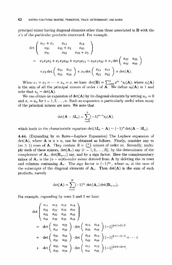
62 MATRIX FUNCTIONS. INVERSE, TRANSPOSE, TRACE, DETERMINANT, AND NORM
principal minor having diagonal elements other than those associated in B with the x's of the particular products concerned. For example,
a21 a22 + 52 a23
a3 1 a32 a33 + 2 3
all $51 a12
det (
When x1 = 52 = . . . = 5, = 5, we have det(B) = C:=, d-Zsi(A), where si(A) is the sum of all the principal minors of order i of A. We define so(A) = 1 and note that s, = det(A).
We can obtain an expansion of det(A) by its diagonal elements by setting aii = 0 and xi = aii for i = 1 , 2 , . . . , n. Such an expansion is particularly useful when many of the principal minors are zero. We note that
n
det(A - XI,) = C(-X)n-isi(A), i = O
which leads to the characteristic equation det(X1, - A ) = (-l),det(A - XI,).
4.44. (Expanding by m Rows-Laplace Expansion) The Laplace expansion of det(A), where A is n x n, can be obtained as follows. Firstly, consider any m (m 2 1) rows of A. They contain R = (;) minors of order m. Secondly, multi- ply each of these minors, det(A,) say (T = 1 , 2 , . . . , R) , by the determinant of the complement of A,, det(B,-,) say, and by a sign factor. Here the complementary minor of A,. is the (n - m)th-order minor derived from A by deleting the m rows and columns containing A,. The sign factor is (-1)"., where a, is the sum of the subscripts of the diagonal elements of A,. Then det(A) is the sum of such products, namely
R
det(A) = c ( - l ) " r det(A,) det(B,-,). T = l
For example, expanding by rows 2 and 3 we have
a12 a13 a14
det [ ii: z:: zt: ) a41 a42 a43 a44
PERMANENTS 63
Further extensions of the Laplace expansion method are available, many of which are named after their originators-for example, Cauchy, Binet-Cauchy (Harville [1997: 200-2021 and Rao and Rao [1997: 149]), and Jacobi.
A number of other expansions are available. For example, if we are interested in relating minors of submatrices, we can use Sylvester’s Determinantal Identity (Rao and Rao [1998: 151-1531). If C = AnxpBpxn, we can expand det C in terms of the sum of products of a minor of A times a minor of B using the Cauchy-Binet formula (Rao and Bhimasankaram [2000: 2381 and Rao and Rao [1997: 1401).
4.45. Given the skew-symmetric matrix
then det(A) = ( a f - be + cd)’.
4.46.
The above matrix occurs in genetics.
Proofs. Section 4.4.4.
4.43. Searle [1982: 1061.
4.44. Harville [1997: section 13.81 and Searle [1982: 1091.
4.46. Quoted by Searle [1982: 1141.
4.5 PERMANENTS
Definition 4.8. Let A be an n x n real matrix. The permanent of A, denoted by per(A), is defined by
n
?r i = l
where 7r is a permutation of the ordered set { 1 , 2 , . . . , n} and ~ ( i ) is the i th mem- ber of the permutation T ; the summation extends over all permutations T . This definition may be compared with the definition of a determinant. There ny=l is multiplied by either +l or -1 depending on whether T is an even or odd per- mutation. Note that per(A) can also be defined for an m x n matrix. For general references to permanents see Wanless [2007] and Minc [1978, 19871, and for an em- phasis on applications in probability and statistics see Bapat [1990]. Permanents can be used to prove a number of properties shared by doubly stochastic matrices.
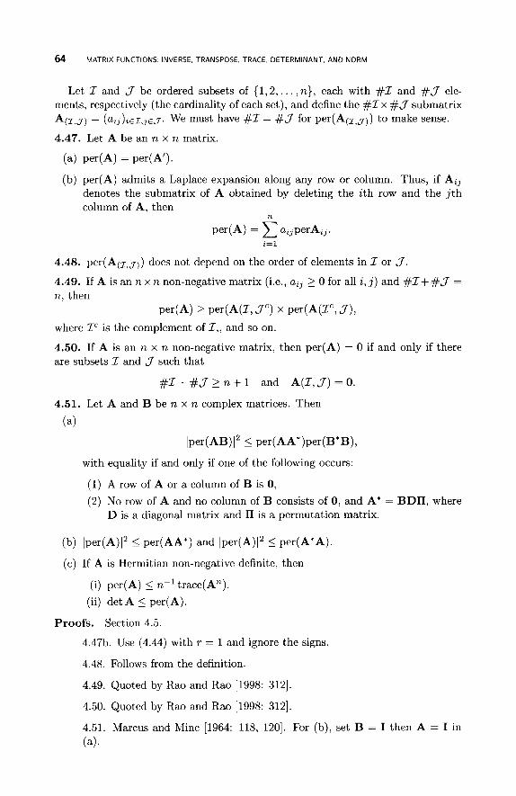
64 MATRIX FUNCTIONS INVERSE, TRANSPOSE, TRACE, DETERMINANT, AND NORM
Let Z and J be ordered subsets of {1,2, . . . ,n}, each with #Z and #J ele- ments, respectively (the cardinality of each set), and define the #Zx #J submatrix A(I,Jl = ( u ~ , ) ~ ~ z , ~ ~ J . We must have #I = # J for per(A(I,J,) t o make sense.
4.47. Let A be an n x n matrix.
(a) per(A) = per(A').
(b) per(A) admits a Laplace expansion along any row or column. Thus, if A,, denotes the submatrix of A obtained by deleting the i t h row and the j t h column of A, then
n
per(A) = 1 %3PerAz,. z = 1
4.48. per(A(I,Jl) does not depend on the order of elements in Z or J .
4.49. If A is an n x n non-negative matrix (i.e., uz, 2 0 for all i, j ) and #Z+ #J = n, then
where Zc is the complement of I,, and so on.
4.50. If A is an n x n non-negative matrix, then per(A) = 0 if and only if there are subsets Z and J such that
per(A) L per(A(Z, J " ) x per(A(Z", J ) ,
# T + # J > n + l and A(Z , J )=O.
4.51. Let A and B be n x n complex matrices. Then
(a)
I per(AB) l 2 5 per(AA*)per( B*B),
with equality if and only if one of the following occurs:
(1) A row of A or a column of B is 0,
(2) No row of A and no column of B consists of 0, and A* = BDrI, where D is a diagonal matrix and 11 is a permutation matrix.
(b) Iper(A)I2 5 per(AA*) and Iper(A)I2 1. per(A*A).
(c) If A is Hermitian non-negative definite, then
(i) per(A) 5 n-' trace(An).
(ii) det A 5 per(A).
Proofs. Section 4.5.
4.47b. Use (4.44) with T = 1 and ignore the signs.
4.48. Follows from the definition.
4.49. Quoted by Rao and Rao [1998: 3121.
4.50. Quoted by Rao and Rao [1998: 3121.
4.51. Marcus and Minc [1964: 118, 1201. For (b), set B = I then A = I in
(4.
NORMS 65
4.6 NORMS
Norms, both for vectors and matrices, are used for measuring distance in vector spaces and for providing a measure of how close one matrix is to another. They can therefore be used for finding the best approximation of a matrix in a given class of matrices by a matrix in another class (e.g., of lower rank). They can also be used for investigating limits of matrix sequences and series. Norms, therefore, have a role to play in statistics in the areas of inequalities, optimization, matrix approximation, matrix analysis, and numerical analysis.
4.6.1 Vector Norms
Definition 4.9. A vector norm on a real or complex vector space U is a real-valued function 11 . I( satisfying the following three conditions.
( I ) jlxll 2 0 for all x E U, and llxll = 0 implies that x = 0 (positive definite property).
(2) llaxll = la1 . llxll for all a E F and all x E U (scalar multiplication).
(3) IIx + yII 5 llxll + llyll (triangle inequality).
A vector norm is said to be unitarily invariant if llUxll = llxll for all x E Cn and all n x n unitary matrices U.
If (1) above is replaced by
( l a ) llxll 2 0 for all x E U,
then 11 . 1 1 is called a vector seminorm.
4.52. The following hold for both a norm and a seminorm for any x, y E U.
(a) / I - XI1 = IIXII.
(b) I llxll - IlYll I 5 IIX - YII.
(c) IIX - YII 5 llxll + IlYll.
4.53. Every vector norm on R" or @" is uniformly continuous.
4.54. For finite-dimensional real or complex vector spaces, all vector norms are equivalent in the sense that if 1 1 . and ( 1 . (10 are two vector norms, then there exist positive constants c1 and c2 such that
c1lIxlIa I IlXllB I c211xIIa
for all x (cf. (4.56) below for some examples).
Definition 4.10. If p is a real number with p 2 1 and x is an n x lvector, then
66 MATRIX FUNCTIONS INVERSE, TRANSPOSE, TRACE, DETERMINANT, AND NORM
is a norm on R" or Cn called the L, norm. Letting p + m, we find that
Ilxll, = max I G lsi<n
is also a norm called the L , norm. The norms most commonly used are the L1, Lz, and L, norms. In particular, the so-called Euclidean norm Lz is used to define the length of a vector in Rn or C". The function llxll, is not a norm for 0 < p < 1.
4.55. The L, norm ( p 2 1) is a vector norm.
4.56. For all x E @" we have:
(a) n-1/211x111 L llxllz I IlXlI1.
(b) IIxIlm I llxllz I ~1/211x11~.
(c) llxll2 I lblll I n1/211Xllz.
(4 IlXllm 5 IlXlll 5 ~IIXII,.
4.57. Every inner product induces a norm; we simply put llxll = (x,x)'l2. How- ever, there are norms not induced by an inner product as in (4.58~) below.
4.58. (Parallelogram Law)
(a) The norm induced by an inner product on a vector space (cf. 4.57) has the property
IIX + Y112 + IIX - Y1I2 = 211x112 + 211Y112.
(b) Conversely, any norm on a real or complex vector space satisfying the above equation is induced by an inner product, namely
(X,Y) = ;(IIx+Y1lZ - llx112 - llY112)~
k Y ) = i ( l l X + Y1I2 - IIX - Y1I2).
An alternative inner product that can be used is
(c) If the parallelogram rule does not hold, then there is no inner product that induces the norm.
(d) Let 1 5 p 5 m. Then the L, norm satisfies (a) if and only if p = 2. Thus L1, for example, does not satisfy (a) so it cannot be induced by an inner product.
4.59. The sum of two vector (semi)norms is a vector (semi)norm, and any positive multiple of a vector (semi)norm is a also a vector (semi)norm.
4.60. Let 1 1 . I l a and I ( . 118 be vector norms on a real or complex vector space V . The function 1 1 . 11 defined by
llxll = max{llxlla? Ilxlla)
is a vector norm.
NORMS 67
4.61. (Continuity) If {x,} and {y,} are sequences of vectors in an inner product space such that IIx, - x I I + 0 and lly, - yII + 0 as n + cm, then
(4 llxnll + llxll and IlYnll + IlYll.
(b) (XmYn) + ( X > Y ) , if llxll < and llYll < 03. 4.62. If 1 1 . 11 is a vector norm on @" and R is a nonsingular n x n matrix, then 1 1 . I I R defined by
IIxlIR = IIRXII, E @"
is also a vector norm on C".
Proofs. Section 4.6.1.
4.52a. By (2) of Definition 4.9.
4.52b. Horn and Johnson [1985: 2601.
4 .52~. By (3) of Definition 4.9 with y replaced by -y.
4.53-4.54. Horn and Johnson [1985: 271, 2721.
4.55. Conditions (1) and (2) of Definition 4.9 are readily verified (cf. Gentle [1998: 71]), and (3) follows from Minkowski's inequality (12.17a).
4.56. (b)-(d) are quoted by Golub and Van Loan [1996: 531, while (a) and (b) are proved by Rao and Bhimasankaram [2000: 258; see the solution to exercise 141.
4.57. Rao and Bhimasankaram [2000: 2561.
4.58a. This follows by simply expanding (x + y, x + y), and so on.
4.58b. Horn and Johnson [1985: 263, exercise 101 and Meyer [2000a: 290-2921,
4 .58~. Abadir and Magnus [2005: 641.
4.58d. Rao and Bhimasankaram [2000: 258; see the solution to exercise 91.
4.59-4.60. Horn and Johnson [1985: 2681.
4.61. Abadir and Magnus [2005: 651.
4.62. Horn and Johnson [1985: 2681.
4.6.2 Matrix Norms
Definition 4.11. We can interpret the word "vector" as simply an element of a vector space. In this case, an rn x n complex matrix A = (a i j ) is simply an element of the space of rn x n complex matrices. Alternatively, this space can also be identified with the vector space Cmn by arranging the entries of each A as an rnn-tuple in some order (e.g., vec A). When a norm applied to vec A satisfies the conditions of a vector norm, we call the norm a generalized matrix norm. Some examples follow.
68 MATRIX FUNCTIONS: INVERSE, TRANSPOSE, TRACE, DETERMINANT, AND NORM
4.63. (Generalized Matrix Norms) Let A be an m x n matrix. Then the following are generalized matrix norms:
(a) IIA1Im = maxl i i jm, l i j sn laijl.
(b) IIA(IF = [ t r a ~ e ( A * A ) ] l / ~ = (EL, E,”=, ~ u ~ ~ ~ 2 ) 1 ~ z l the Frobenius norm. (We use a subscript F instead of F = 2 to avoid confusion later in dealing with matrix norms instead of generalized ones.)
Definition 4.12. (Induced Norms) Given the vector norm 1 1 . [ I v , the generalized matrix norm induced by 1 1 . I I v for the m x n matrix A is defined by
where x E @”. As noted by Horn and Johnson [1985: 2921, we can replace ‘Lsup’l by “max” in the above definition. The most common vector norms are the L, norms with p 2 1. Note that 1 1 . I I F is not an induced norm, and is not to be confused with II ‘ 112,in (cf. 4.66b).
4.64. The induced norm IIAllv,in is a generalized matrix norm as condition (3) of Definition 4.9 in Section 4.6.1 holds.
4.65. If A is m x n and B is n x q, then for an L, vector norm ( p 2 1)
IIABll,,in I IIAllP,inllBll~,in
This result does not hold for every 1 1 . Ilv,in. Golub and Van Loan [1996: 551, in quoting the above result, note that it represents a relationship between three different norms defined on Rmxql RmXn and Rnxq, respectively. They also call the above norm a matrix norm, which it is for square matrices (see Definition 4.13 below).
4.66. Let A be m x n. Then following are induced norms based on Lp vector norms.
(a) IlAll1,in = max1ijin cz1 lazjl.
(b) IIAllz,in = [A,,,(A*A)]’/2 = amax(A), where A,,, is the maximum eigen- value of A*A and amax is the maximum singular value.
(c) IIAllm,ia = max1si<m c;=, bijl. 4.67. If A is m x n then:
(a) IIAl12,in 5 llAll~ 5 n1/211Al12,in. (See also (4.82) below for square matrices.)
(b) maxl l ism,ls jsn laijl I IAl12,in I (mn)’/2 maxl i i im, l s j sn laijl.
(c) m-1’211AIIi,in I I I ~ l I z , i n I n1’211AIIi,in.
(d) n-”211Allm,in I IIAll2,in I m1’211Allca,in.
NORMS 69
The above bounds on the norm IIAl12,in are useful, because this norm is more difficult to compute than either IIAlll,in or IIAllm,in.
Definition 4.13. Let V be the vector space of n x n complex matrices. If A E V , then the matrix n o m of A , denoted by lllAlll, is any real-valued non-negative function of A satisfying the following conditions.
(1) lllAlll 2 0 and lllAll1 = 0 if and only if A = 0.
(2) lllcAlll = IcI . lllAlll, where c i s any scalar and IcI is its modulus.
(3) If B E V then IIIA + Blll 5 IllAlll + IIIBIII.
(4) If c E V then IllAClll 5 IllAlll ' IllCllll.
Note that the first three conditions are those of a generalized matrix norm (and of a vector norm), which can be applied to any m x n matrix. However, condition (4) applies to square matrices only. For a brief introduction to matrix norms see Meyer [2000a: section 5.21.
4.68. Let 1 1 1 . 1 1 1 be any matrix norm and A any n x n matrix.
(i) p(A) 5 lllAlll, where p is the spectral radius.
(ii) p(A) = l im~+m(~llAkll~) ' 'k.
(i) From AI, = A and Definition 4.13(4) we have lllI,lll 2 1.
(ii) Repeated use of Definition 4.13(4) give us IIIAkllI 5 (lllAlll)k ( k a posi-
(iii) Using AA-' = I , and Definition 4.13(4) gives us IIIA-llll 2 ( ~ ~ ~ A ~ ~ ~ ) - l .
(c) From A = (A - B) + B, Definition 4.13(3), and interchanging the roles of A
(a)
(b)
tive integer).
and B, we have I IllAlll - IllBlll I L 111-4 -Bill. (d) Ja,jl 5 BlllAlll for all i and j , where 6 = maxl<i<, , l~j<, IIIEijIII, and Eij is
(e) If II(Allls = JIIS-lASIII for all nonsingular n x n matrices S, then lllAllls is
an n x n matrix with 1 in the i , j t h position and zeros elsewhere.
a matrix norm.
4.69. Let A be an n x n matrix.
(a) llAllp = (Crzl Cy=l(laZjlp)llp is a matrix norm for 1 5 p 5 2. When p = 2
la i j ( ) is a matrix norm, but llAllco of (4.63a)
we use the notation IIIAIIIp.
max (b) If n 2 2 , IlAll = n(l<i<n.l<j<n
is not, though it is a generalized matrix norm.
4.70. Result (4.69b) above can be generalized. For every generalized matrix norm IIAlla, where A is n x n, there is a finite positive constant c, which depends on the norm such that c,llAll, is a matrix norm.
70 MATRIX FUNCTIONS- INVERSE, TRANSPOSE, TRACE, DETERMINANT, AND NORM
4.71. An n x n matrix A is nonsingular if there is a matrix norm 1 1 1 . 1 ) ) such that 1111, - All1 < 1. In this case
k=O
4.72. Given E > 0, there exists a matrix norm ( 1 1 . 1 1 1 such that
p(A) I IllAlll < P(A) + 6 ,
where p is the spectral radius (see also 4.68a).
Definition 4.14. The generalized matrix norm induced by the vector norm 1 1 . for the square matrix A is a matrix norm because it satisfies the four conditions of Definition 4.13. We call it the induced matrix norm and we denote it by IIIAlllv,in
For further discussion of this norm see Horn and Johnson [1985: 292-2951 and Rao and Rao [1998: 367-81.
4.73. For n x R matrices, the induced matrix norm has the following properties.
(4 IIIInlllv,in = 1.
(b) IlAxllv I IIIAlllv,in ' llxllv
(c) lll~Alllv,in = I4 . lllAlllv,in.
(4 I l l - AIIIv,in = IIIAlllv,in
(el IIII, +AlIl.,i, I IIIInlllv,in + IIIAlllv,in = 1 + IIIAlllv,in
(f) I I I L - Alllv,in I 1 + lllAlllv,in.
(g) Suppose IIIAlllv,in < 1.
(i) B = I, - A and I, + A are nonsingular.
(ii) From B(In - A) = I, we can take the norm of B = I, + BA using (e) and Definition 4.13(4) to get
By replacing A by -A and using (c) above we see that the same bounds apply for lll(In + A)-llllv,zn.
4.74. Let A be an n x n matrix. The matrix norm induced by an L, vector norm is given by
IIIAlII,,zn = ,,I$:l IIAXllP, P 2 1.
Setting p = 1,2 , m, we have:
( 4 IIIAlll1,zn = max113sn C L 14. (b) IIIAlllz,zn = [X,,,(A*A)]1/2 = cmax(A), where A,,, is the maximum eigen-
value of A*A and omax is the maximum singular value. We note that A,,, is
NORMS 71
real and non-negative as A'A is Hermitian and non-negative definite. We note that A,,,, = p(A"A), where p is the spectral radius. When A is Hermitian, lllA1112,in = [p(A2)]'I2, which reduces to p(A) when A is also non-negative definite. For further properties of this induced norm see Meyer [2000a: 281-2831. This matrix norm is also called the spectral matrix norm.
(c) IIIAlllco,in = m a x l l i ~ n c;=, bijl. The inequalities given in (4.67) apply to the above matrix norms by setting m = n.
4.75. If A and B are non-negative definite n x n matrices, then:
(a) IIIASBS1112,in I IIIABlll;,in for 0 I s I 1.
(b) If ~~lABll12,in I 1, then IIIASBS1112,in I 1 for 0 I s I 1.
(c) IIIABllli,in I IIIAtBtll12,in for t L 1.
4.76. Let 11 . and 11 . 110 be two given vector norms on @", and let 1 1 1 . I(Ia,in
and 1 1 1 . IIlp,in denote the respective induced matrix norms on the space V of n x n matrices.
(a) Define IIXIIB
x+o I I x I I a Rap = max ~ l l X l l a and Rpa, = max -.
X # O IIXIIP
Then
(b) IIIAllla,zn = I I I A ~ ~ ~ O , ~ ~ for all A E V if and only if there is a positive constant c such that /lxlla = cl lx l lp for all x E @.
(c) lllAllla,zn I IIIAIIIp,zn for all A E V if and only if llAlla,2n = IIAIIP,~~ for all A E V
4.77. If Q is unitary (or orthogonal), then:
(a) 11Q~112 = IIxIIz (b) l l lQI l l2 ,zn = 1.
Definition 4.15. A matrix norm I I I . I I I on the class of n x n matrices is a mznimal matrzx norm if the only matrix norm N ( . ) such that N ( A ) I lllAlll for all A is
= I l l ' I l l . 4.78. Every induced norm is minimal and every minimal norm is induced.
Definition 4.16. If A is m x n, the Frobentus norm is defined to be
IlAll~ = (XF; la,,12)'/2 = [ t r a ~ e ( A * A ) ] ' / ~ = IIA*II.v. 2 3
When m # n, this norm is a generalized matrix norm, while if m = n, it is a matrix norm. However. it is not an induced norm. It is often refered to as the Euclidean
72 MATRIX FUNCTIONS: INVERSE. TRANSPOSE, TRACE. DETERMINANT, AND NORM
matrix norm as l l lAll l~, like IIIA1112,in, uses an Lz vector norm. For this reason, Graybill [1983], for example, uses E , but we shall follow the general trend and use the subscript F t o avoid confusion. Harville [1997] refers t o the Frobenius norm as the “usual norm.” Even when m # n, the following result shows that the norm satisfies a result like (4) of Definition 4.13.
4.79. If A is rn x n and B is n x p , then l l A B l l ~ 5 I~AI(F. llBllp.
4.80. If A is m x n of rank r with singular values L T ~ = cri(A), then
r
llAll$ = trace(A*A) = trace(AA*) = c;. i= l
4.81. Given real symmetric A and real skew-symmetric B, both n x n, then
IIIA + B1112F = lllAlll2F + 111B1112F
4.82- lllA1112,in 5 lllAlllF 5 filIIAl112,in.
4.83. If A and U are n x n and U is unitary, then
IIIAlll2,in = lllUAlll2,in = IIIAU1112,in = IIIU*AU1112,in.
The above also holds for 1 1 1 . ( 1 1 ~ . Proofs. Section 4.6.2.
4.63. Rao and Rao [1998: 3631. The results follow by applying (4.55) to vec A .
4.64. We see that llAx + Ayllv 5 llAxllv + llAyllv implies that max llAx + AyllT, I max{ llAxllv + IIAyllV> 5 max llAxllv + max IIAyllv.
4.65. Quoted by Golub and van Loan [1996: 551.
4.66. Horn and Johnson [1985: 294-295, the proofs hold for m # n] and Meyer [2000a: 281-2841.
4.67. Golub and Van Loan [1996: 56-57].
4.68a(i). Horn and Johnson [1985: 2971, Meyer [2000a: 4971, and Rao and Rao [1998: 3651.
4.68a(ii). Horn and Johnson [1985: 2991, Meyer [2000a: 6191, and Rao and Rao [1998: 3731.
4.6%. Horn and Johnson [1985: 2901.
4.68d. Rao and Rao [1998: 3651.
4.68e. Horn and Johnson [1985: 2961.
4.69a. Graybill [1983: 93, p = 11, Horn and Johnson [1985: 291, p = l , 2 ] , and Rao and Rao [1998: 3741.
4.69b. Horn and Johnson [1985: 2921.
NORMS 73
4.70. Horn and Johnson [1985: 3231.
4.71. Horn and Johnson [1985: 3011. See also (19.16a) using an infinite series.
4.72. Horn and Johnson [1985: 2971 and Rao and Rao [1998: 3721.
4.73a-c. Horn and Johnson [1985: 2931 and Rao and Bhimasankaram [2000: 259; see the solution to exercise 151.
4.73d. Since IIAxllzl = 11 - Axilv.
4.73e. From sup(a + b) 5 sup a + sup b.
4.73f. Follows from (d).
4.73g. Rao and Bhimasankaram [2000: 259; see the solution to exercise 151.
4.74a. Horn and Johnson [1985: 2941 and Rao and Rao [1998: 3701.
4.74b. Rao and Rao [1998: 3711.
4 .74~. Horn and Johnson [1985: 2951 and Rao and Rao [1998: 368-3691,
4.75. Bhatia [1997: 255-2561,
4.76. Horn and Johnson [1985: 303-305, further results are given there in section 5.61.
4.77. Gentle [2000: 731.
4.78. Horn and Johnson [1985: 3061.
4.79. Harville [1997: 4321.
4.80. From the singular value decomposition of A, crf is the i th ordered eigenvalue of A A ” and the trace is the sum of the eigenvalues.
4.81. Rao and Rao [1998: 3901
4.82. Since A’A is non-negative definite it has non-negative eigenvalues A, and trace(A*A) = C,X,. The result then follows from A,,, 5 C,A, 5 nA,,,, and taking square roots.
4.83. Gentle [1998].
4.6.3 Unitarily Invariant Norms
Definition 4.17. A real-valued function 11 . I / on the vector space V of m x n complex matrices is said to be a uni tar i ly i nvar ian t (generalized m a t r i x ) norm, and denoted by / I . 1 1 u 2 , if it has the following properties. We shall drop the words “generalized matrix” below.
(1) /\All 2 0 for all A E V and IlAll = 0 if and only if A = 0.
(2) llaAl1 = lalllAl1 for every a E C and A E V .
74 MATRIX FUNCTIONS: INVERSE, TRANSPOSE, TRACE, DETERMINANT, AND NORM
(3) I(A + BII 5 llAl( + l(Bll for all A and B in V .
(4) ((UAVII = IlAll for all A E V and unitary matrices U and V of orders m x m and n x n, respectively.
Thus a generalized matrix norm, which satisfies the first three conditions, is uni- tarily invariant if it satisfies (4) as well. If m = n and I(ABI1 5 llAllllBll for all n x n matrices, then 11 . 1 1 is a matrix norm that we denote by 1 1 1 . l l l u z .
If V is the space of real matrices, then we use the term orthogonally znwamant norm.
4.84. Let 11 . matrices. Then:
be a unitarily invariant norm defined on V , the space of m x n
(a) llAB*1IuZ I al(A)IIBIIuz for all A,B E V .
IlAlluz 2 ~l(A)IIE1111uz for all A E V . (b) If Ell is the matrix with 1 in the (1,l) position and zeros elsewhere, then
Here a1(A) is the maximum singular value of of A.
4.85. A unitarily invariant norm 1 1 . l l u z on the space V of n x n matrices is a matrix norm if and only if IIAlluZ 2 a1(A) (= IIIAlI12,zn) for all A E V . An equivalent condition from (4.84b) above is llElllluz 2 1. Note that Bhatia [1997: 911 uses the sufficient condition llElllluz = 1 in his definition of matrix norm, which leads to a slightly different norm.
Definition 4.18. We define the term general square root of the m x n complex matrix A to be the unique non-negative definite matrix (A*A)’/2 (cf. 10.8), and denote it by IAl.
4.86. Let A be an m x n matrix. Since (A*A)’I2 has the same singular values as A, which are the same as those of A* (cf. 16.34d), then from (4.87) below we have
I I IAl l l u z = llA11uz
for all unitarily invariant norms
4.87. Let A = PEQ* be the singular value decomposition of an m x n matrix A, where X is diagonal and P and Q are unitary m x m and n x n matrices, respectively. Then
IlAlluz = IIP*P~Q*QIIuz = lIXlluz>
which is a function of the singular values of A. The nature of this function is discussed below.
4.88. Let A be an m x n matrix.
(a) The Frobenius norm IlAll~ = (ELl Cj”=, laij12)1/2 and IIA112,in = omaz (the maximum singular value of A) are both unitarily invariant generalized matrix norms. When m = n they are both unitarily invariant matrix norms.
(b) I(AJ12,in is the only unitarily invariant norm that is also an induced norm.
NORMS 75
Two other classes of unitarily invariant norms that seem to be of particular interest are the Ky Fan k-norms and the Schatten pnorms (Bhatia [1997: 921 and Horn and Johnson [1985: 441, 4451).
4.89. Suppose A and B belong to the vector space V of m x n matrices and let p = min{m,n}. In order that llAllzLz 5 11B112n for every unitarily invariant norm
1 1 . l lzLz on V , it is sufficient that
a,(A) 5 a,(B) for all i = 1 , 2 , . . . , p ,
and it is necessary and sufficient that
a1(A) + . . . + a,(A) 5 o ~ ( B ) + . . . + o,(B), i 1 1 , 2 , . . . , p .
We now introduce a function, called a symmetric gauge function, which is inti- mately related to the unitarily invariant matrix norm. In fact, IlAll is a unitarily invariant norm if and only it is a symmetric gauge function of the singular values of A (cf. (4.87) and (4.92)).
Definition 4.19. A real-valued function 4 from R" to R is said to be a symmetric gauge function if it has the following properties.
(1) 4(x) > 0 for all x E R" with x # 0.
(2) q5(cyx) = Icyld(x) for all x E R" and cy E R.
(3) 4(x + y) 5 d(x) + $(y) for all x and y in R"
(4) 4(xT) = $(x) for all x E R" and all permutations x, of the elements of x.
( 5 ) ~ ( J x ) = 4(x) for all x E R" and all diagonal matrices J with diagonal elements $1 or -1. This is equivalent t o 4(x) = 4(mod x), where mod x =
(1x21).
4.90. The following hold.
(a) From (1) to (3) above, 4 is a vector norm on R".
(b) A symmetric gauge function is continuous.
(c) The sum of two symmetric gauge functions is a symmetric gauge function
(d) A positive multiple of a symmetric guage function is a symmetric gauge func- tion.
(e) The L, vector norm ( p 2 1) on R" is a symmetric gauge function.
For some examples of symmetric gauge functions, their properties, and some in- equalities see Bhatia [1997: chapter 41.
4.91. Let 4 be a symmetric gauge function, and let x = (xi) E R".
(a) If y = (yi) = (pixi), where 0 5 pi 5 1 for all i, then
d ( Y l , . . . , Y n ) I4(x1 , . . . ,x71)
76 MATRIX FUNCTIONS. INVERSE, TRANSPOSE, TRACE, DETERMINANT, AND NORM
(b) If 0 5 xi 5 yi for all i, then
n
,xn) 5 k ( c Izil), where k = 4(1,0,0, . . . i= 1
4.92. Let 1 1 . ll,i be any unitarily invariant norm on the vector space V of m x n real matrices, and let p = min{m, n}. For each x = (xi) E R" let X,,, = diag(x) and ~ ( z I , . . . ,x,) = IIXll,i. Then 4 is a symmetric gauge function. Thus from (4.87), with X replacing X, we have that IIAll,i = d(al(A), .2(A), . . . , op(A)), where 4 is a symmetric gauge function and .i(A) is the i th singular value of A.
Conversely, if 4 is a symmetric gauge function on RP, then the function defined
by IlAll = 4(.1(A),.Z(A), . . . ,.p(A))
is a unitarily invariant norm on V . Unitarily invariant norms and gauge functions have been found useful in multi-
variate analysis in relation to monotone properties of power functions and simulta- neous confidence intervals (Mudholkar [1965, 19661 and Wijsmann [1979]).
4.93. The n x n matrix A has the same singular values as A* so that by (4.86) above, IIAll,i = JIA*llui for all A and all unitarily invariant norms. Such a norm is called a self-adjoint norm.
4.94. (Ky Fan) np 2 0 and CT; 2 oh 2 . . . 2 .; 2 0 are two sets of values, then
If 4 is a symmetric gauge function on RP and CT~ 2 02 2 . . . 2
$( .I , . . . , .p) 2 4(.;,. . . ,.;I if and only if
0 1 + .. . +.z 2 0; +. . . +.:, 2 = 1 ,2 , . . . , p .
Proofs. Section 4.6.3.
4.84. Horn and Johnson [1991: 2061.
4.85. Horn and Johnson [1985: 450; 1991: 211, exercise 31.
4.87. Rao and Rao [1998: 3751.
4.88a. Rao and Rao [1998: 3761.
4.88b. Horn and Johnson [1985: 3081.
4.89. Horn and Johnson [1985: 4471 and Rao [1980: 61.
4.90. Rao and Rao [1998: 377-3781.
4.91. Rao and Rao [1998: 377-3781.
4.92. Horn and Johnson [1985: 438-441; 1991: 2101 and Rao and Rao [1998: 378-3801,
4.94. Fan [1951].
NORMS 77
4.6.4 M , N-Invariant Norms
Definition 4.20. Let M be a given positive definite m x m matrix and N a given n x n positive definite matrix. A generalized matrix norm on the space V of m x n matrices is said to be an M,N-invariant norm if, in addition to conditions ( l) , (2), and ( 3 ) of Definition 4.17 in the previous section, it satisfies the following condition
IJVAUI/ = IlAll for every A E V ,
and any m. x m matrix V and any n x n matrix U such that V"MV = M and U*NU = N. This norm was introduced by Rao [1979,1980] to deal with dimension- reducing techniques in multivariate analysis. When M and N are the identity matrices, the M , N-invariant norm becomes the unitarily invariant norm.
4.95. Using the above notation, let M1/2, M-1/2 N'/2 and N-'/2 be the respec- tive positive definite square roots of M, M-l, "and N-l (cf. 10.32). Then the following hold.
(a) If llAlla is a unitarily invariant norm of A, then llM1/2AN1/211a is an M , N- invariant norm of A.
(b) If IlAllp is an M , N-invariant norm of A, then I(M-1/2AN-1/211p is a unitarily invariant norm of A.
Proofs. Section 4.6.4.
4.95. Rao and Rao [1998: 394-3951, They also give a number of matrix approximations based on the M , N-invariant norm.
4.6.5 Computational Accuracy
An important question in computing is: How do errors both in the da ta and in the round-off affect the computation of expression-for example, the inverse of a nonsingular matrix? Suppose A is n x n and, instead of computing A-l, we actually compute (A + dA)-'. Then, assuming that a particular matrix norm of the error IlbAll is small enough, Horn and Johnson [1985: 335-3381 show that if 11bAlllJA-'(l < 1, then
where &(A) = IJAIJIIA-l11. The above expression bounds the relative error in the inverse in terms of the relative error in the data. For lldAll small, the right-hand side of the above expression is of the order of K ( A ) ~ ~ ~ A ~ ~ / ~ ~ A / ~ . Therefore if &(A) is not large, the relative error in the inverse is of the same order as the relative error of the data.
One can obtain a similar result in computing an eigenvalue. For example, if i is an eigenvalue of A + bA, where A is diagonalizable (e.g., symmetric) with A = RAR-l and A = diag(A1,. . . , A n ) , then there is some eigenvalue X i of A such that, for an appropriate matrix norm,
I i - Ail 5 llRllllR-lllll~All = K(R)IIbAtI.
78 MATRIX FUNCTIONS: INVERSE, TRANSPOSE, TRACE, DETERMINANT, AND NORM
Horn and Johnson [1985: section 6.31 derive a number of perturbation results like the one above for different properties of A and 6A.
Finally, we look at a corresponding result in relation to solving linear equations. For example, consider
Duff et al. [1986: 89-90] show that if 116AllIIA-111 < 1, then
(A + 6A)(x + 6x) = b + 6b.
In introducing K(A) in the above discussion, we have not specified the norm I ( . 1 1 . Furthermore, in deriving the above expression it transpires that we only require the norm to be an induced one. Also, the definition of K(A) used above is only appropriate for nonsingular matrices. By choosing an appropriate norm, we now generalize the definition to include nonsingular and rectangular matrices.
Definition 4.21. The condition number of an m x n real matrix A, denoted by 4 A ) , is the ratio of the largest singular value to the smallest nonzero singular value. Thus,
1/2
tc2(A)= (h) Amin
where A,,, is the largest and Amin is the smallest nonzero eigenvalue of A'A. Unfortunately, this condition number is not easy to compute, and for further details see Gentle [1998: 115-1161.
4.96. When A is positive definite, its eigenvalues are positive, A'A = A', and
The same is true for a Hermitian positive definite A, as we replace A'A by A*A. Some bounds on 6 2 are given in (6.21b).
4.97. If A is nonsingular, then
K.2(-4) = IIIAlll2,in . IIIA-11112,in>
where 1 1 1 . 1112,in is the induced matrix norm corresponding to the L2 vector norm (cf. 4.74b).
We can also define K ~ ( A ) and nm(A) corrresponding to the L1 and L , norms.
4.98. If v = 1,2, or cm, then:
(a) K,(A) = K ~ ( A - ' ) .
(b) K,(cA) = fiv(A) for c # 0.
(c) nv(A) L 1.
(d) &i(A) = K ~ ( A )
(el K2(A) = K.Z(A').
(f) K~(A'A) = KZ(A) 2 Q(A).
Proofs. Section 4.6.5.
4.98. Gentle [2000: 781.
CHAPTER 5
COMPLEX, HERMITIAN, AND RELATED M AT R I C E S
Although complex matrices have been refered to in previous chapters, it seems ap- propriate to have a chapter that looks more closely at complex matrices. Complex matrices arise, for example, in time series and the related topic of signal process- ing, and in experimenal designs. We shall initially list some general properties of complex matrices before looking at Hermitian matrices. The related matrices that are considered are the skew-Hermitian, complex symmetric, real symmetric, skew-symmetric, complex orthogonal, and normal matrices. Factorizations and decompositions for these matrices are given in Chapter 16, while results about eigenvalues and eigenvectors for these matrices are located in Chapter 6. Unitary and real orthogonal matrices are considered in greater detail in Section 8.1, and Fourier matrices are covered in Section 8.12.2. At the end of this chapter we briefly consider quaternions, which are used, for example, in nuclear physics.
5.1 COMPLEX MATRICES
Definition 5.1. Given a complex number x = x1 +ixz, where x1 and x2 are both real, then its complex conjugate is defined to be ?E = x1 - 2x2, and its modulus or absolute value is defined to be 1x1, where 1x1 = (x: + x ; ) ~ / ~ . If A is complex, it can be expressed in the form A = A1 + iA2, where A1 and A2 are real matrices, and its complex conjugate is = A1 - iA2. We also define the conjugate transpose of A to be A* = A’.
A M a t n x Handbook for Statisticzans. By George A. F. Seber Copyright @ 2008 John Wiley & Sons, Inc.
79
80 COMPLEX, HERMITIAN, AND RELATED MATRICES
Definition 5.2. An n x n matrix A is said to be a Hermitian matrix if A* = A and skew-Hermitian (anti-Hermitian) if A = -A”.
A real or complex matrix A is symmetric if A = A’. A complex orthogonal n x n matrix T is a complex matrix such that T’T = I,.
An n x n matrix U is called a unitary matrix if U*U = I,. We omit the word “complex” if T is real.
5.1.1 Some General Results
5.1. For complex scalars 3: and y we have:
(4 l ZY l = b l l Y I . (b) I2 + YI 5 I4 + IYI.
(c) /x i2 + IyI2 2 2Re(xjj), where Re is the “real part.”
5.2. A complex orthogonal matrix T need not be unitary.
5.3. (Isomorphism Between Complex and Real Matrices) Let Z = Z1+ iZ2 be an n x n complex matrix with Z, (i = 1,2) real matrices. Let
Z R = ( ;; -;$ and define XR and YR in a similar fashion.
(a) If Z = X + Y, then ZR = XR + YR.
(b) If Z = XY, then ZR = X R Y R .
(c) If W = Z - l , then W R = (ZR)-’ .
(d) det ZR = I det Z12.
(e) If Z is Hermitian, then ZR is symmetric.
( f ) If Z is unitary, then ZR is orthogonal.
(g) Suppose the eigenvalues and eigenvectors of Z are A, and aj = a13 + i a 2 j ,
j = 1 , 2 , . . . , n, where the a,, are real for r = 1,2 , and all j. Then those of zR are, respectively,
This result could be useful for carrying out numerical computations involving complex matrices.
5.4. Let x = ( ~ 1 ~ x 2 , . . . ,zn)’ be a complex vector with I Cy=l zil = C,”=, 1x21. Then zi = 6’lx21, i = 1 , 2 , . . . ,n, for some complex number 6’ satisfying 16’1 = 1.
5.5. If A is a square complex matrix and x*Ax = 0 for all complex x, then A = 0. Thus if x*Ax = x*Bx for all complex x, then A = B. However, these results do not necessarily hold if the matrices are real and the equalities hold for all real x.
COMPLEX MATRICES 81
5.6. If A is an n x n real or complex matrix, then there exists a nonsingular matrix S such that SAS-’ is symmetric. There also exists a nonsingular matrix R such that A’ = RAR-’
5.7. Let A be an n x n real or complex matrix. Then every product of n entries of A taken from distinct rows and columns equals 0 (i.e., a l z , , a222 . . . anz, = 0), with distinct i,, if and only if A contains an T x s zero submatrix, where T + s = n + 1.
5.8. Let A = (az,) be an n x n real or complex matrix with eigenvalues A, (i = 1 ,2 , . . . , n ) , then
n n
~ I X Z l 2 5 Fy)Z312. 2 = 1 z=1 ,=1
Equality occurs if and only if A is normal (cf. Section 5.6).
Proofs. Section 5.1.1.
5.1. Abadir and Magnus [2005: 121.
5.2. For a 2 x 2 counterexample see Horn and Johnson [1985: 71, exercise 81.
5.3. Quoted by Brillinger [1975: 711 with a corrected sign change. All the results except (c) and (d) can be verified directly, while (c) amounts to showing that if WZ = I then WRZR = I; (d) follows from (5.10).
5.4. Bapat arid Raghavan [1997: 191.
5.5. Davis [1979: 61-62]. For a counter example see (5.25).
5.6. Horn and Johnson [1985: 209-2101
5.7. Zliang [1999: 126-1271
5.8. Zhang [1999: 2601
5.1.2 Determinants
5.9. Let A = A1 +iA2, where A1 and A2 are real n x n matrices. If det A = a+ib and I . I represents the modulus, then:
(a) det A = a - ib.
(b) det A’ = det A.
det AI2 = I det XI2 = a2 + b2 = I det A det XI = det A det A.
de tAde tAl = IdetAdetA’l = Idet(AA’)l = Idet(AA*)I.
Let
A = A l + i A 2 , B = ( ) and C = -A2 A1
82 COMPLEX, HERMITIAN. AND RELATED MATRICES
where A1 and A2 are real matrices. Then, for det A l # 0,
det B = det C and I det A1 = I det BI1/’ = 1 det C1’/’.
Proofs. Section 5.1.2.
5.9. The results (a)-(c) follow from the definition and the product rule for determinants, and (d) follows from the expansion of a determinant.
5.10. Mathai [1997: 171-1721.
5.2 HERMIT IAN MATRICES
5.11. An n x n matrix A is Hermitian if and only if one (and therefore all) of the following five conditions hold.
(1) x*Ax is real for all x E C”.
(2) A2 = A’A.
(3) trace(A2) = trace(A*A).
(4) A is normal and all the eigenvalues of A are real
( 5 ) S*AS is Hermitian for all n x n S.
5.12. Suppose A is an n x n Hermitian matrix. Then the following hold.
(a) A k is Hermitian for k = I, 2 , . . ..
(b) i A is skew-Hermitian.
(c) If A is nonsingular, then A-l is Hermitian
(d) The diagonal elements of A are real.
(e) The eigenvalues of A are real (see Section 6.1.6 for further details).
5.13. Let A be an n x n matrix.
(a) A can be expressed uniquely in the form A = S + iT, where S and T are Hermitian.
(b) A can be expressed uniquely in the form A = B + C , where B is Hermitian and C is skew-Hermitian.
5.14. (Complex Householder Matrix) If A = I, - 2bb*, where b is a complex n x 1 vector such that b*b = 1, then A is Hermitian, unitary (i.e., A * A = In), and involutionary (i.e., A’ = I,).
5.15. (Trace) If A is n x n, then:
(a) trace(AX) = 0 for all Hermitian matrices X if and only if A = 0.
(b) trace(AX) is real for all Hermitian X if and only if A is Hermitian.
SKEW-HERMITIAN MATRICES 83
5.16. A square matrix A is a product of two Hermitian matrices if and only if it is similar to A*.
Proofs. Section 5.2.
5.11. Zhang [1999: 2091 proves (1)-(3), while Horn and Johnson [1985: 170- 1711 prove (l), (4), and (5).
5.12. Horn and Johnson [1985: 169-1701.
5.13a. Horn and Johnson [1985: 1701. We set A = $(A+A*)+i[-$(A-A')], and assume two such representations.
5.13b. Set A = ;(A + A*) + ;(A - A*).
5.15. Rao and Rao [1998: 3421.
5.16. Zhang [1999: 2151.
5.3 SKEW-HERMITIAN MATRICES
5.17. A - A* is skew-Hermitian for all square matrices A.
5.18. Let A be skew-Hermitian.
(a) iA is Hermitian.
(b) The diagonal elements of A are all purely imaginary.
(c) Since the eigenvalues of an Hermitian matrix are real, the eigenvalues of A (and therefore of a real skew-symmetric matrix) are purely imaginary or zero.
(d) (I, + A) is nonsingular
5.19. Suppose A is a skew-Hermitian n x n matrix. Then, using (5.18d) above, we have:
(a) U = (I, - A)(I, +A)- ' = (I, +A)- '& - A) is unitary as U*U = I,.
This follows from (I, - A)(I, + A) = (I, + A)(I, - A).
(b) U = [2I, - (I, + A ) ] & +A)- ' .
(c) From (a) we see that I, - A and (I, + A)-' commute.
(d) I, + U is nonsingular because, by (b), it equals 2(I, + A)-1.
(e) The matrices U and A are in (1, 1)-correspondence on account of the pair of equations
U = 2(I,+A)-' -I,,
A = 2(I, +U)-l -I,.
Thus A is skew-Hermitian if and only if U is unitary.
84 COMPLEX, HERMITIAN, AND RELATED MATRICES
( f ) These results hold if A is (real) skew-symmetric and U is real orthogonal.
Apparently the above results were first applied to statistics by Hsu [1953].
Proofs. Section 5.3.
5.18a. (iA)* =;A* = ( - i ) ( -A) = ZA.
5.18b. Use (a) and (5.12d).
5 .18~. Use (5.12e)
5.18d. The determinant of a matrix is the product of its eigenvalues. Also, X(1, + A) = 1 + X(A) = 1 + i a # 0, as from (c) a is real or zero.
5.4 COMPLEX SYMMETRIC MATRICES
Although real symmetric matrices play a fundamental role in statistics, we shall first consider some results that hold for both real and complex symmetric matrices. Note that real symmetric matrices are also Hermitian (Section 5.2), normal (Section 5.6), and diagonalizable (Section 16.1), so that the results in those sections also apply to symmetric matrices.
5.20. We assume that A is an n x n real or complex matrix.
(a) A is symmetric if and only if there exists an n x n matrix S such that A = SS'.
We may choose S = UD, where U is unitary,
D = d iag ( f i , 6,. . . , Jan), and the LT~ are the singular values of A, in which case
rank S = rank A.
(b) If A is symmetric, then A is diagonalizable (cf. Definition 16.3) if and only if it is complex orthogonally diagonalizable. Thus A = SAS-' for a diagonal matrix A of eigenvalues of A (cf. 16.17a) if and only if A = QAQ', where Q is an n x n complex orthogonal matrix (i.e., Q'Q = In).
5.21. If A and B are real or complex symmetric n x n matrices, then there exists a nonsingular n x n matrix R such that A = RBR' if and only if rank A = rank B.
5.22. By considering a 2 x 2 matrix, we see that the eigenvalues values of a complex symmetric matrix are not necessarily real.
Proofs. Section 5.4.
5.20a. Horn and Johnson [1985: 2071.
5.20b. Horn and Johnson [1985: 211-2121.
5.21. Horn and Johnson [1985: 2251
5.22. For a counterexample, Abadir and Magnus [2005: 1751 consider
which has eigenvalues 1 f i .
REAL SKEW-SYMMETRIC MATRICES 85
5.5 REAL SKEW-SYMMETRIC MATRICES
Definition 5.3. A matrix A is said to be skew-symmetric if A’ = -A. Note that a complex matrix like
where a is complex, is skew-symmetric. However, my focus is on real matrices as they are a special case of skew-Hermitian matrices; some of the properties in Section 5.3 will then apply for real matrices. For a factorization of a real skew-symmetric matrix see (16.46b(ii)).
5.23. The diagonal elements of a real skew-symmetric matrix are all zero.
5.24. Let A be an n x n real skew-symmetric matrix.
(a) From (5.18c), the eigenvalues X,(A) of A are zero or purely imaginary and occur in conjugate pairs, as the characteristic polynomial has real coefficients. Hence the eigenvalues take the form *ia, with a, real (i = 1 ,2 , . . . , p ) , along with (n - 2p) zeros. Thus:
( i ) If n is odd, det(A) = 0.
(ii) If n is even, det(A) 2 0.
(iii) det(1, + A ) = n:==,(l + &(A)) 2 1 with equality if and only if A = 0.
(b) Let 71 = 2m, then det(A) is the square of a polynomial of degree m in the matrix entries ( e g , (4.45)). The polynomial is called the p f a f i a n of A and is denoted by Pf(A). There are two ways of defining a pfaffian and a helpful resource is http://en.wikipedia.org/wiki/Pfaffian. We have:
(i) det(A) = [Pf(A)]’.
(ii) Pf(BAB’) = det(B)Pf(A).
(iii) Pf(cA) = cmPf(A).
(iv) Pf(A’) = (-l)’”Pf(A).
(v) For an arbitrary m x m matrix C ,
Pf ( ) = (-l)m(m-1)/2det(C). -C’ 0
For further references see Halton [1966b], Mehta [2004: 543-545, examples of computation] and Northcott [1984].
5.25. Let A be a real square matrix and x a real vector, then x’Ax = 0 for all x if and only if A is skew-symmetric.
Proofs. Section 5.5.
5.23. Follows from (5.18b)
5.24a(i). The determinant of a matrix is the product of its eigenvalues.
5.24a(ii). ( ia) ( - ia) = a’, where a may be zero.
COMPLEX. HERMITIAN. AND RELATED MATRICES 86
5.6
5.24a(iii). Use (5.18d) and (1 + ia)(l - ia) = 1 + a2.
5.24b. Quoted in http://en.wikipedia.org/wiki/Pfaffian. Depending on the definition used, several proofs are available for (i) (originally due to Cay- ley); for example, Parameswaran [1954], Dress and Wenzel [1995], and Halton [1966a]. Serre [2002: 22-23] proves (ii).
5.25. Davis [1979: 60-611.
NORMAL MATRICES
Definition 5.4. A square matrix A is said to be normal if AA* = A'A. Note that Hermitian, skew-Hermitian, and unitary matrices are all normal, as are their real counterparts.
5.26. An n x n matrix A with eigenvalues XI, A 2 , . . . . , A, is normal if and only if there exists a unitary matrix Q such that
Q*AQ = diag(Xl,A2, . ..,A,).
We say that A is unitarily diagonalizable. Note that this applies to Hermitian and unitary matrices (see also (16.46)).
5.27. If A is a commuting family of n x n normal matrices (i.e., AlA:! = A2Al for all A l , A2 E A), then every member of A is unitarily diagonalizable by the same unitary matrix.
5.28. In addition to being unitarily diagonalizable, normal matrices have many unique properties, some of which are listed below. The following statements are equivalent.
(1) A is normal.
(2) There exists a polynomial p ( z ) of degree at most n - 1 such that A* = p(A).
(3) The singular values of A are lAl(A)I, IA2(A)I,.. . , lA,(A)l.
(4) A = R + i s , where R and S are real, symmetric, and commute (i.e., RS =
SR).
(5) Every eigenvector of A is an eigenvector of A*
(6) There exists a set of eigenvectors of A that form an orthonormal basis for C".
(7) ci cj la2A2 = ci lAi(A)I2.
5.29. If A is normal and p ( z ) is a polynomial, then p(A) is normal.
5.30. An upper-triangular matrix is normal if and only if it is diagonal.
5.31. A normal matrix is unitary if and only if its eigenvalues have absolute value 1.
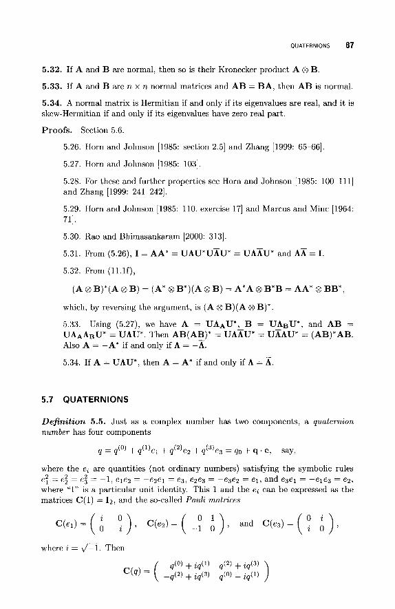
QUATERNIONS 87
5.32. If A and B are normal, then so is their Kronecker product A @ B.
5.33. If A and B are n x n normal matrices and AB = BA, then AB is normal.
5.34. A normal matrix is Hermitian if and only if its eigenvalues are real, and it is skew-Hermitian if and only if its eigenvalues have zero real part.
Proofs. Section 5.6.
5.26. Horn and Johnson [1985: section 2.51 and Zhang [1999: 65-66].
5.27. Horn and Johnson [1985: 1031.
5.28. For these and further properties see Horn and Johnson [1985: 100-1111 and Zhang [1999: 241-2421,
5.29. Horn and Johnson [1985: 110, exercise 171 and Marcus and Minc [1964: 711.
5.30. Rao and Bhimasankaram [ZOOO: 3131.
5.31. From (5.26), I = AA* = UAU*UnU* = UAnU* and AX = I.
5.32. From (ll.lf),
(A @ B)*(A @ B) = (A* @ B*)(A @ B) = A*A @ B*B = AA' @ BB*,
which, by reversing the argument, is (A @ B)(A @ B)*.
5.33. Using (5.27), we have A = UA*U*, B = UABU*, and AB = UA~A,U* = UAU*. Then AB(AB)* = UAKU* = UKAU* = (AB)*AB. Also A = -A* if and only if A = -x. 5.34. If A = UAU*, then A = A* if and only if A = n.
5.7 QUATERNIONS
Definition 5.5. Just as a complex number has two components, a quaternion number has four components
say, q = q ( O ) + q (1) el + q(2)e2 + q(3)e3 = qo + q . e ,
where the ei are quantities (not ordinary numbers) satisfying the symbolic rules , 2 - 2 - 2 - - e2 - e3 - -1, e1e2 = -e2e1 = e3, e2e3 = -e3e2 = e l , and e3e1 = -e1e3 = e2, where "1" is a particular unit identity. This 1 and the ei can be expressed as the matrices C(l) = 12, and the so-called Pauli matrices
where i = &f. Then
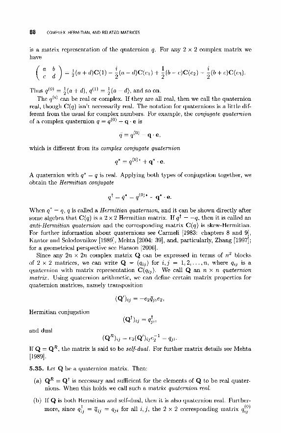
88 COMPLEX, HERMITIAN. AND RELATED MATRICES
is a matrix representation of the quaternion q. For any 2 x 2 complex matrix we have
Thus q ( O ) = $ ( a + d ) , q(’ ) = ; (a - d ) , and so on. The q( i ) can be real or complex. If they are all real, then we call the quaternion
real, though C ( q ) isn’t necessarily real. The notation for quaternions is a little dif- ferent from the usual for complex numbers. For example, the conjugate quaternion of a complex quaternion q = q ( O ) + q . e is
q.e, q = q(o) -
which is different from its complex conjugate quaternion
q* = q ( O ) * + q* . e .
A quaternion with q* = q is real. Applying both types of conjugation together, we obtain the Hermitian conjugate
qt = q* = q(0 )* - g* . e.
When qt = q, q is called a Hermitian quaternion, and it can be shown directly after some algebra that C ( q ) is a 2 x 2 Hermitian matrix. If qt = -q, then it is called an anti-Hermitian quaternion and the corresponding matrix C ( q ) is skew-Hermitian. For further information about quaternions see Carmeli [1983: chapters 8 and 91, Kantor and Solodovnikov [1989], Mehta [2004: 391, and, particularly, Zhang [1997]; for a geometrical perspective see Hanson [2006].
Since any 2 n x 2 n complex matrix Q can be expressed in terms of n2 blocks of 2 x 2 matrices, we can write Q = ( q i j ) for i , j = 1 , 2 , . . . , n, where qi3 is a quaternion with matrix representation C(qz j ) . We call Q an n x n quaternion matrix. Using quaternion arithmetic, we can define certain matrix properties for quaternion matrices, namely transposition
( Q ’ ) . . - - - 23 - e24jie2,
Hermitian conjugation t
(Qt)ij = q j z ,
and dual (QR) . . - e2(Q’). . -l = 4..
If Q = QR, the matrix is said to be self-dual. For further matrix details see Mehta [ 19891.
5.35. Let Q be a quaternion matrix. Then:
21 - 23 e2 3 2 .
(a) QR = Qt is necessary and sufficient for the elements of Q to be real quater- nions. When this holds we call such a matrix quaternion real.
(b) If Q is both Hermitian and self-dual, then it is also quaternion real. Further- more, since qt . = ijij = q j i for all i , j , the 2 x 2 corresponding matrix q/30)
23
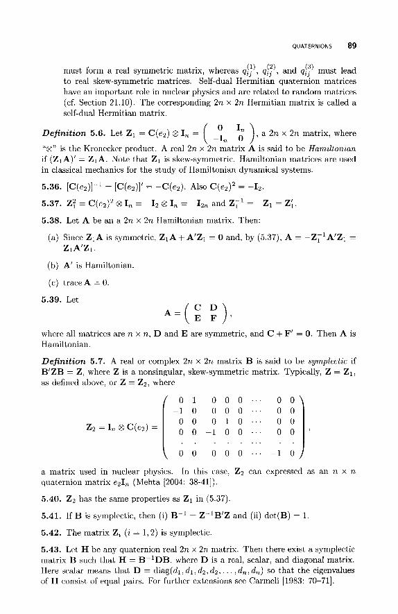
QUATERNIONS 89
must form a real symmetric matrix, whereas &), qj;), and q(3) must lead to real skew-symmetric matrices. Self-dual Hermitian quaternion matrices have an important role in nuclear physics and are related to random matrices (cf. Section 21.10). The corresponding 2n x 2n Hermitian matrix is called a self-dual Hermitian matrix.
Definition 5.6. Let Z 1 = C(e2) @I, = ( _”,, ), a 2n x 2n matrix, where
“8” is the Kronecker product. A real 2n x 2n matrix A is said to be Hamiltonian if (ZlA)’ = Z1A. Note that Z1 is skew-symmetric. Hamiltonian matrices are used in classical mechanics for the study of Hamiltonian dynamical systems.
5.36. [C(e2)]-’ = [C(ez)]’ = -C(e2). Also C(e2)’ = -12.
5.37. Z; = C(e2)’ @ I, = -12 8 I, = -12, and Z;’ = -Z1 = Zi
5.38. Let A be an a 2n x 2n Hamiltonian matrix. Then:
”.
(a) Since Z1A is symmetric, Z1A+ A’Z1 = 0 and, by (5.37), A = -Z,’A’Z1 = Z1A‘ZI.
(b) A’ is Hamiltonian.
(c) traceA = 0.
5.39. Let C D
. = ( E F ) ’
where all matrices are n x n, D and E are symmetric, and C + F’ = 0. Then A is Hamiltonian.
Definition 5.7. A real or complex 2n x 2n matrix B is said to be symplectic if B’ZB = Z, where Z is a nonsingular, skew-symmetric matrix. Typically, Z = Z1,
as defined above, or Z = Z2, where
0 1 0 0 0 ’ ” 0 0 -1 0 0 0 0 “ ’ 0 0
2 2 = I, @ C(e2) =
0 0 0 0 0 . ’ . -1 0
a matrix used in nuclear physics. In this case, Z2 can expressed as an n x n quaternion matrix e21, (Mehta [2004: 38-41]).
5.40. 2 2 has the same properties as Z1 in (5.37).
5.41. If B is symplectic, then (i) B-’ = Z-lB’Z and (ii) det(B) = 1
5.42. The matrix Zi ( i = 1,2) is symplectic.
5.43. Let H be any quaternion real 2n x 2n matrix. Then there exist a symplectic matrix B such that H = B-lDB, where D is a real, scalar, and diagonal matrix. Here scalar means that D = diag(d1, dl , dz, dz, . . . , d,, d,) so that the eigenvalues of H consist of equal pairs. For further extensions see Carmeli [1983: 70-711.
90 COMPLEX, HERMITIAN, AND RELATED MATRICES
Proofs. Section 5.7.
5.36-5.37. These are straightforward; we use ( l l . l e ) , ( l l . l i ) , and (11.11).
5.3813. Taking transposes in (a) and using (5.37), we have A' = Z1AZ1.
5 .38~ . Using (a), traceA = - trace(ZT'A'Z1) = -trace A' = -trace A.
5.39. Show that Z1A is symmetric.
5.40. Zg = I, 8 C ( ~ Z ) ~ = -I, 8 12 = -12,.
5.41. The result (i) follows from the definition by multiplying on the left by Z-' and on the right by B-', and (ii) follows from (5.24b(ii)).
5.42. (ZiZi)Zi = (Zi'Zi)Zi = Zi.
5.43. Carmeli [1983: 701.
CHAPTER 6
EIGENVALUES, EIGENVECTORS, AND SINGULAR VALUES
Eigenvalues, eigenvectors, and singular values play an important role in statistics, and they arise in most of the chapters in this book. In this chapter we deal with these topics in a general sense. They also occur in a number of important inequal- ities in this chapter, in Chapter 14, and in Chapter 23 on majorization, and they underlie many of the factorizations and decompositions in Chapter 16. For those relating to specific matrices and some patterned matrices, the reader will need to refer to the index for those matrices. This chapter closes with a a brief introduction to antieigenvalues and antieigenvectors, which are becoming of increasing interest to statisticians in recent years.
6.1 INTRODUCTION AND DEFINITIONS
Definition 6.1. Let A be an n x n matrix, which we assume to have elements in F (i.e., either R or @, unless otherwise stated). The polynomial c(X) = det(A - XI,) is called the characteristic polynomial. The equation c(X) = 0 is called the characteristic equation, and its roots are called the eigenvalues (characteristic roots, latent roots) of A. Many authors use f ( X ) = det(X1, - A) = (-l),det(A - XI,) for the characteristic polynomial, as the coefficient of A" is now 1. This alternative version is sometimes more convenient, so both c(.) and f( .) are used below.
Eigenvalues may be real, complex, or a mixture of both. We shall order the eigenvalues by their modulus values, i.e., 1x11 2 lXzl 2 . . . 2 IX,I 2 0. If XI is unique, we shall call it the dominant eigenvalue. In this case there exists a unique
A M a t n x Handbook for Statistacians. By George A. F. Seber Copyright @ 2008 John Wiley & Sons, Inc.
91
92 EIGENVALUES, EIGENVECTORS, AND SINGULAR VALUES
right eigenvector XI of unit length such that Ax1 = Alxl, called the dominant eigenvector.
The s distinct eigenvalues are denoted by p1, p2,. . . , ps (or p j (A) , j = 1,2 , . . . , s), where > Ipzl > . . . > /psi 2 0. The set of pj is called the spectrum of A , and p(A) = l p l / = / A l l is called the spectral radius. We can therefore write f (A ) = nj=l(A - p ~ j ) ~ ~ , where C& mj = n. Here mj [or m ( p j ) ] is called the al- gebraic multiplicity of the eigenvalue pu,. If mj = l , pj is called a simple eigenvalue, while if rnj > 1, pj is called a multiple eigenvalue.
For every pj there exists a nonzero solution x such that Ax = pjx, and x is called an eigenvector associated with p j . The set of all such x together with 0, namely N ( A - pjI,) the null space of A - pjITL, is called the eigenspace of p j . The dimension gj [or g(pu,)] of this space is called the geometric multiplicity of p j . To avoid ambiguity, we shall refer t o such an x as a right eigenvector. There similarly exists a nonzero y such that y'A = pjy' called the left eigenvector of A associated with pu,.
If rn(pj) = g ( p j ) , then p3 is said to be a semisimple eigenvalue.
6.1. (Multiplicities). Let A be an n x n matrix.
(a) g ( p j ) 5 m ( p j ) ; that is, the geometric multiplicity is no greater than the algebraic multiplicity.
(b) rank(A - pjI,) = n - g ( p j ) 2 n - m ( p j ) for all j .
(c) If m ( p j ) = 1 so that p j is a simple eigenvalue, then g ( p j ) = 1 and rank(A - pjIn) = n-1. Conversely, if rank(A-p,I,) = n- 1, then pL3 is an eigenvalue, but not necessarily a simple eigenvalue.
Proofs. Section 6.1
6.la. Schott [2005: 891 and Rao and Bhimasankaram [2000: 2861
6.lb. From (3.3a), dimC(B)+dimN(B) = n for B = A-pjI,, as dimC(A*) = rankA' = rankA = dimC(A).
6 . 1 ~ . Magnus and Neudecker [1999: 201.
6.1.1 Characteristic Polynomial
Definition 6.2. (Symmetric Functions) Given a set of constants XI,. . . , A n , we define the elementary symmetric funct ions as
n
INTRODUCTION AND DEFINITIONS 93
Also, let .(A) = (- l )"(An + a1Xn-' + . . . + a,-lX +a,) = ( - l ) " f ( X ) be the characteristic polynomial.
6.2. If the characteristic polynomial has real coefficients, then any complex eigen- values must come in conjugate pairs.
6.3. (Cayley-Hamilton theorem) f (A) = 0
6.4. The coefficient a, ( r = 1 , 2 , . . . , n) is (-1)' times the sum of all the r x r principal minors of A. These are obtained by striking out n - r rows and the same numbered columns of A and taking the determinant of the remaining submatrix.
(a) a, = (-l)'S, ( r = 1 ,2 , . . . ,n ) with a, = (-1)" det A.
(b) From (a), S, is the sum of all the r x r principal minors of A.
(c) If t , = X;+X;+. . .+A; for r = 1 ,2 , . . . ,n and we define 0 = a,+l = an+2 = . . ., then t ,+t,-lal+. . .+tla,-l +m, = 0 ( r = 1 ,2 , . . .). These expressions for the a , are known as Newton's identities (Hunter [1983a: 156-1571).
6.5. If A is n x n, and p is not an eigenvalue of A, then A - p1, is nonsingular as its determinant is nonzero.
6.6. If A, B, and R are n x n matrices, and B = RAR-' (i.e, A and B are similar), then A and B have the same characteristic polynomial. Note that having the same eigenvalues is a necesssary but not sufficient condition for similarity.
6.7. If A and B are real n x n matrices, then the eigenvalues of
A B ' = ( B A )
are those of A + B and A - B.
Definition 6.3. I f f is a polynomial such that f (A) = 0, we say that f annihilates A. A polynomial is said to be monic if the coefficient of the highest power is unity.
6.8. If A is n x n, there exists a unique monic polynomial of minimum degree no greater than n that annihilates A.
Definition 6.4. The monic polynomial q ( X ) of the least degree that annihilates A is called the minimal polynomial.
6.9. Every monic polynomial is both the minimal polynomial and the characteristic polynomial ( f (A) version) of its companion matrix (cf. 6.14).
6.10. The minimal polynomial divides every polynomial that annihilates A. It therefore divides the characteristic polynomial f (A) (by 6.3).
6.11. If q ( X ) is the minimal polynomial of A, then X is a root q(X) = 0 if and only if it is an eigenvalue of A. Thus every root of the characteristic equation is a root of q ( A ) = 0.
6.12. If A, B, and R are n x n matrices, then A and the similar matrix B = RAR-' have the same minimal polynomial.
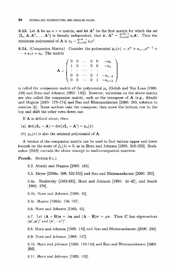
94 EIGENVALUES. EIGENVECTORS, AND SINGULAR VALUES
6.13. Let A be an n x n matrix, and let Ak be the first matrix for which the set {In, A, A 2 , . . . , A t } is linearly independent, that is, Ak = C::; a , A Z . Then the
minimum polynomial of A is xk -
6.14. (Companion Matrix) . . . + alx + ao. The matrix
a,x~.
Consider the polynomial pn(x) = xn + an-lxn-l +
0 0 . . . 0 0 -a0
A = [ ! 0 : : : 0 0 -ul 1 0 0 ” . 0 1 -an-2 0 0 . ’ . 0 1 -an-l
is called the companion matrix of the polynomial p , (Golub and Van Loan [1996: 3481 and Horn and Johnson [1985: 1461). However, variations on the above matrix are also called the companion matrix, such as the transpose of A (e.g., Abadir and Magnus [2005: 173-1741 and Rao and Bhimasankaram [2000: 283, solution to exercise 31). Some authors take the transpose, then move the bottom row to the top and shift the other rows down one.
If A is defined above, then:
(a) det(z1, - A) = det(x1, - A’) = p,(x).
(b) pn(x) is also the minimal polynomial of A.
A version of the companion matrix can be used to find various upper and lower bounds on the roots of fn(X) = 0, as in Horn and Johnson [1985: 316-3201. Bosh- nakov [2002] extends the above concept to multi-companion matrices.
Proofs. Section 6.1.1
6.2. Abadir and Magnus [2005: 1641.
6.3. Meyer [2000a: 509, 532-5331 and Rao and Bhimasankaram [2000: 2921.
6.4a. Basilevsky [1983:192], Horn and Johnson [1985: 41-42], and Searle [1982: 2781.
6.4b. Horn and Johnson [1985: 421.
6 . 4 ~ . Hunter [1983a: 156-1571.
6.6. Horn and Johnson [1985: 451.
6.7. Let (A + B)u = X u and (A - B)v = pv. Then C has eigenvectors (u’, u’)’ and (v’, -v’)’.
6.8. Horn and Johnson [1985: 1421 and Rao and Bhimasankaram [2000: 2931.
6.9. Horn and Johnson [1985: 1471.
6.10. Horn and Johnson [1985: 142-1431 and Rao and Bhimasankaram [2000: 2931.
6.11. Horn and Johnson [1985: 1431.
INTRODUCTION AND DEFINITIONS 95
6.12. Horn and Johnson [1985: 1431 and Rao and Bhimasankaram [2000: 2951.
6.13. Meyer [2000a: 6431.
6.14. Meyer [2000a: 6481.
6.1.2 Eigenvalues
We asume that A is n x n,
6.15. For every j, and A real or complex:
(a) &(A') = Aj(A).
(b) Xj(A) = Xj(A).
( c ) Xj(A*) = X,.(A).
(d) Xj(K-'AK) = Xj(A) for all j.
6.16. If A has r nonzero eigenvalues, then:
(a) rankA 2 r
(b) It is possible to have r = 0, but have rankA = n - 1.
6.17. We have the following:
(a) If k is a positive integer, then
n
trace = C i=l
(b) Taking k = 1, traceA = Cy=l Xi.
(c) det(A) = ny=l X i .
6.18. A is nonsingular if and only if Aj(A) # 0 for all j (cf. 6 .17~) .
6.19. If A is triangular, then, since the determinant of the upper-triangular matrix A - XI, is the product of its diagonal elements, the eigenvalues are the diagonal elements of A.
6.20. If A, = 0 is the only zero eigenvalue, then
n-1
trace(adjA) = rl[ Xi, i = l
where adjA is the adjoint matrix of A.
96 EIGENVALUES, EIGENVECTORS, AND SINGULAR VALUES
6.21. (Bounds Using Traces) Let A be an n x n real or complex matrix with real eigenvalues X i ; for example, A is Hermitian or symmetric. Define
1 " 1 m = - x & = - t r a c e A n n
i = l
and 1 " 1
s2 = -(x A:) - m2 = - trace(A2) - m2. n
i=l
(a) Then
m - s(n - 1)1/2
m + s(n - 1)-'/2 5 5
X,in(A) 5 m - s(n - 1)-'I2,
Xma,(A) 5 m + s(n - 1)'I2.
Equality on the left (respectively right) of the first equation holds if and only if equality holds on the left (respectively right) of the second equation, if and only if the n - 1 largest (respectively smallest) eigenvalues are equal. When n = 2 we have Xmin(A) = m - s and X,,,(A) = m + s.
(b) (Bounds on the Condition Number) Let A be Hermitian positive definite with condition number K ~ ( A ) = XmaxA/Xmin(A) (cf. 4.96).
(i) When n is even,
When n > 2 , equality holds if and only if A = cI,, where c is a real constant.
(ii) When n is odd, (i) holds along with
When n = 3, equality holds if and only if the two smallest eigenvalues are equal. When n > 3, equality holds if and only if A = cI,.
(iii) In general,
( 2 ~ ~ ) ' / ~ s [ m + s(n - I ) - ' / ~ ] ~ - ' det A K2(A) 5 1 +
When n > 2 , equality holds if and only if A = cI,.
A is positive definite, (i) holds, and (iv) If A is Hermitian, trace A > 0, and (traceA)2 > (n - 1) trace(A2), then
When n > 2 , equality holds if and only if A = cI,.
INTRODUCTION AND DEFINITIONS 97
(c) Suppose A has real eigenvalues with f eigenvalues of A positive and g nega- tive. Let trace(A2) > 0.
(i) When traceA 2 0, then
(traceA)'/trace(A2) 2 f ,
with equality if and only if all the positive eigenvalues are equal and all the nonpositive eigenvalues are equal.
(ii) When traceA 5 0, then
(traceA)2/ trace(A2) 5 g,
with equality if and only if all the negative eigenvalues are equal and all the non-negative eigenvalues are equal.
(d) Let A1 2 A2 2 . . . 2 A,.
(i) Then
Equality occurs if and only if
(ii) From (i) we have ~1 - A, 5 ( 2 n ) ' / 2 s .
When n > 2 , equality holds if and only if
1 A2 = A3 = . . . = A,-1 = z ( A 1 + An).
(iii) If R = 2q is even, then 2 s 5 A1 - A,,
with equality if and only if
(iv) If R = 2q It 1 is odd, the previous inequality (iii) holds and
2 s n ( n 2 - 1)-'12 5 ~1 - A,,
with equality if and only if the conditions for the equality of (iii) hold.
(v)
(trace A)2 (A1 + A d 2 trace(A2) - A; + A; '
< n - 2 +
98 EIGENVALUES, EIGENVECTORS, AND SINGULAR VALUES
When n > 2, equality holds if and only if A1 + A, # 0 and
(e) The above results can be extended to complex matrices with complex eigenval- 2 . . . 2 IA,J ues. For example, if A now has complex eigenvalues l A l l 2
and we define
1 1 n n
m = - traceA and s% = - trace(A*A) - lmI2,
then:
(i) Iml - s,(n - 1)l/' 5 ]A,[ 5 [ t ra~e(A*A)/n] ' /~ .
Equality holds on the left if and only if A is normal, A1 = A2 = . . . = and A, = cm for some real non-negative scalar c 5 1. Equality
holds on the right if and only if A is normal and 1x1 I = 1 A21 = . . . = ]A,[.
(ii) Iml 5 1x11 5 Iml+ s,(n - I)'/'.
Equality holds on the left if and only if A1 = A2 = . . . = A,. Equality holds on the right if and only if A is normal, A2 = A3 = . . . = A,, and A1 = cm for scalar c 2 1.
(iii) If A has lc nonzero eigenvalues, then
I traceAl'/trace(A*A) 5 k 5 rankA.
Equality holds on the left if and only if A is normal and / A l l = 1x21 = . . . = JAkl . Equality holds on the right if and only if rankA = rank(A2).
Further extensions are given by Wolkowicz and Styan [1980].
Additional results relating to sums of eigenvalues are given by Wolkowicz and Styan [1980]. Extensions are given by Merikoski and Virtanen [2004] and are used to give a lower bound for the Perron root of a non-negative matrix.
6.22. Let A = (a i j ) and B = (b i j ) be n x n matrices with eigenvalues X i and -yi, respectively. Define
. n n
then
6.23. Let A and B be real n x n symmetric matrices with C(A) that B is non-negative definite, and let X be an n x lc matrix. Then:
C(B). Suppose
(a) C(X'AX) C C(X'BX).
(b) Consider the eigenvalues of (X'BX)-X'AX for any weak inverse (X'BX)-.
INTRODUCTION AND DEFINITIONS 99
(i) The eigenvalues are all real and do not depend on the choice of general-
(ii) The eigenvalues are the generalized eigenvalues of X’AX with respect
ized inverse.
to X’BX (cf. Section 6.1.8).
(c) Zn[(X’BX)-X’AX)] = In(X’AX), where In ( . ) is the inertia.
6.24. For each 2, A, is a continuous function of the elements of A.
6.25. (Quadratic Inequalities) ( z = 1 , 2 , . . . , n) are a set of mutually orthonormal vectors, i.e., x:xJ = bzJr then:
Suppose A is an n x n Hermitian matrix and x,
k (a) Cz=l x:Axz I E:=l &(A), k = L 2 , . . . ,n - 1
(b) c;=1 x:Axz = c;=1 Az(A)
6.26. (Hirsch and Bendixson) Let A = ( a z J ) be an n x n complex matrix with eigenvalues A,, and define the Hermitian matrices B = (A + A*)/2 and C = (A - A*)/(22). Then:
(a) IA,I I nmaxlazJl.
(b) I%e(A,)l I nmaxlb,,I.
(c) I W A , ) I 5 nmaxIc23I.
2 J
2 ,.I
?.I
Here %e and Csm denote the “real” and “imaginary” parts, respectively. When A is Hermitian, the three results all reduce to (a).
6.27. (Schur) If A = ( a z J ) is an n x n complex matrix with eigenvalues A,, then
n
z = 1 i j
with equality if and only if A is a normal matrix.
6.28. If A is any n x n matrix, then, given E > 0, there exists an n x n matrix B with distinct eigenvalues such that
z = l 3 = 1
6.29. (GerSgorin) Let A = ( a z J ) be an n x n matrix, and let
n
(a) All the eigenvalues of A are located in the union of n discs (called GerSgorin discs)
u;=l{z E c : Iz - a221 5 Ri}.
100 EIGENVALUES. EIGENVECTORS. AND SINGULAR VALUES
Furthermore, if the union of k of these discs forms a connected region that is disjoint from the remaining n - k discs, then there are precisely k eigenvalues in this region.
(b) Since A and A’ have the same eigenvalues, a similar result holds with Ri replaced by
n
and the union of discs by
(c) The eigenvalues of A lie in the intersection of the above two regions.
Some generalizations of the above results are given by Horn and Johnson [1985: section 6.41.
6.30. (Commuting Matrices) Let A be an n x n matrix with distinct eigenvalues, and let B be an n x n matrix that commutes with A , that is, AB = B A . Then B can be expressed uniquely as a polynomial in A with degree no more than n - 1.
6.31. (Perturbations) Suppose that a Hermitian n x n matrix with (real) eigen- values A1 2 . . . 2 A, is perturbed by a Hermitian matrix E with ranked eigenvalues 6 , to give B = A + E with ranked eigenvalues Dz. Then
Proofs. Section 6.1.2
6.15. Abadir and Magnus [2005: 166-1671 and Horn and Johnson [1985: 57,
(a)-(c)l.
6.16a. Graybill [1983: 305]), Magnus and Neudecker [1999: 19-20], and Schott [2005: 1601.
6.16b. For a counter example see Abadir and Magnus [2005: 165, exercise 7.191.
6.17. Schott [2005: 911.
6.20. If A has nonzero eigenvalues, then trace(adjA) = trace[(det A)A-’] = II,A, C, A;’. Let A, + 0.
6.21. Wolkowicz and Styan [1980: (a), 474-476; (b) 484-485; (c) 480-481; (d) 482-483; and (e) 491, 4951.
6.22. Ostrowski [1973]; see also Elsner [1982] for some other bounds.
6.23. Scott and Styan [1985: 2121.
6.24. Schott [2005: 1031.
INTRODUCTION AND DEFINITIONS 101
6.25. Rao and Rao [1998: 3831.
6.26. Marcus and Minc [1964: 1411.
6.27. Marcus and Minc [1964: 1421 and Zhang [1997: 2411; Tsatsomeros [2007: 14.21 also lists this and other inequalities.
6.28. Bellman [1970: 1991.
6.29. Horn and Johnson [1985: 344-3461 and Meyer [2000a: 4981.
6.30. Zhang [1999: 591.
6.31. Meyer [2000a: 5511.
6.1.3 Singular Values
Definition 6.5. Suppose B is an m x n real or complex matrix of rank r , where r 5 p = min(m,n). The p largest eigenvalues of B*B, which are the same as those for BB" (by 6 . 5 4 ~ ) are non-negative (by 10.10 and 10.2), as B'B is non- negative definite. Their positive square roots are called the singular values of B. Denote these by u1 2 u2 2 . . . 2 uT > ur+l = . . . = up = 0; we shall use the notation ut = ui(B). (See Section 16.3 for further details and the singular value decomposition of a matrix.) Some interesting historical comments are given by Horn and Johnson [1991: section 3.01.
6.32. Suppose that B is an m x n matrix with singular values u1 2 u2 2 . . . 2 up 2 0, and p = min{m,n}. Let
0 B* . = ( B 0 )
Then A is an ( m + n) x (m + n) Hermitian matrix with eigenvalues
u1 2 u2 2 ' . . 2 up 2 0 = ' . ' = 0 2 -up 2 -up-1 2 ' . ' 2 -u1,
with Im - n1 zeros in the middle.
6.33. Suppose B E B, the set of all m x n matrices. Then, for every E > 0, there exists B, E B with distinct singular values such that IIB - Bell < E , where 1 1 . 1 1 is any generalized matrix norm on B.
6.34. Let A be an n x n matrix with &(A) and ui(A) the ordered eigenvalues and singular values, respectively, in decreasing order of magnitude.
(a) n,"=, IXi(A)I 5 & ui(A) for k = 1 , 2 , . . . , n, with equality for k = n.
(c) ItraceAl 5 ul(A)+az(A)+...+u,(A) . EqualityholdsifandonlyifA =uC for some non-negative definite matrix C and some complex scalar u with unit modulus. When equality holds, A is a normal matrix.
102 EIGENVALUES, EIGENVECTORS, AND SINGULAR VALUES
(d) a,(A) = a,(UAV) (i = 1,2 , . . . , n) for all n x n unitary matrices U and V.
(e) l i m , , , [ ~ , ( A ~ ) ] ~ / ~ = IX,(A)I for i = 1 , 2 , . . . ,n.
6.35. If A is an n x n matrix and H(A) is the Hermitian matrix ;(A + A*), then, for i = 1 , 2 , . . . , n, the following results hold.
(4 g,(A) 2 Xz(H(A)).
(b) a,(A) 2 X,[H(UAV)] for all n x n unitary U and V.
6.36. If A is an m x n matrix, p = min{m, n} , and a, = a,(A), then:
k k (b) Cz=la22<Cs=~~,, k = 1 , 2 , . . . , p
Equality in (a) holds if and only if the leading k x k principal submatrix of A is diagonal and laz,l = O, (z = 1,2, . . . , k ) . Equality in (b) occurs when equality in (a) holds and a,, 2 0 (i = 1 , 2 , . . . , k ) .
6.37. (Bilinear Inequalities) Let A be an m x n matrix, and let p = min{m,n}. For z = 1 , 2 , . . . ,p , let 2: = (xi, yi) be any mutually orthonormal vectors, where x, is m x 1 and yz is n x 1. Then
k k
i=l i = l
Equality is attained when xi and yi are, respectively, the left and right singular vectors of A associated with ai (cf. Section 16.3).
6.38. Let A be a real or complex square matrix with numerical radius
w(A) = SUP Ix*AxI. IIxII=l
Then p(A) 5 w(A) I amax I 2w(A), where p(A) is the spectral radius of A.
Proofs. Section 6.1.3
6.32. Horn and Johnson [1985: 4181 and Rao and Rao [1998: 3251.
6.33. Horn and Johnson [1985: 4171.
6.34a. Horn and Johnson [1991: 1711 and Rao and Rao [1998: 339-3401.
6.3413. Horn and Johnson [1991: 1761.
6 .34~. Horn and Johnson [1991: 1761 and Zhang [1999: 260-2611.
6.34d. Horn and Johnson [1991: 1461.
6.34e. Horn and Johnson [1991: 1801.
6.35. Horn and Johnson [1991: 1511.
6.36. Rao and Rao [1998: 3851.
6.37. Rao and Rao [1998: 383-3841,
6.38. Zhang [1999: 901.
INTRODUCTION AND DEFINITIONS 103
6.1.4 Functions of a Matrix
6.39. If Ax = X,x and k is a positive integer, then Akx = Xtx, so that Ak has eigenvalues A! and the same eigenvectors as A. If At = 0 for some positive integer t , then &(A) = 0 for all 2.
6.40. If A has eigenvalues X,(A), a polynomial g(A) has eigenvalues g(X,) (i = 1 ,2 , . . . , n) and the same eigenvectors as A.
6.41. If A is nonsingular with eigenvalues A,, then A-l has eigenvalues A;’.
6.42. Let A be an n x n matrix. If ao, u l , . . . ,a, are real or complex numbers, and
B = aoIn + alA + . . . + amAm,
then the eigenvalues of B are
a~+a~p,(A)+a~p~(A)+.~.+a,p,”(A) for j = 1,2, . . . , s,
where the p,(A) are the distinct eigenvalues. If B = 0, then any eigenvalue X of A must satisfy the equation
a0 + U l X + a# + . . . + amXm = 0.
Proofs. Section 6.1.4
6.39. Schott [2005: 901.
6.40. Rao and Bhimasankaram [2000: 2891.
6.41. Schott [2005: 901.
6.42. Quoted by Marcus and Minc [1964: 231.
6.1.5 Eigenvectors
6.43. Right (left) eigenvectors associated with distinct eigenvalues pj are linearly independent.
6.44. The eigenspace corresponding to a distinct eigenvalue p j , say, is a vector subspace.
6.45. Let A be a real or complex square matrix, and let x be any n x 1 nonzero vec- tor. Then there exists an eigenvector y of A belonging to the span of {x, Ax, A’x, . . .} 6.46. (Left and Right Eigenvectors) Suppose A is a complex square matrix.
(a) If Ax = Ax, y*A = py*, and X # p, then x is orthogonal to y (i.e., x*y = 0).
(b) A*y = ,Gy.
Proofs. Section 6.1.5
6.43. Rao and Bhimasankaram [2000: 2871.
6.44. Schott [2005: 881.
6.45. Rao and Bhimasnakaram [ZOOO: 2881 and Rao and Rao [1998: 1841.
6.46. Abadir and Magnus [2005: 1731.
104 EIGENVALUES, EIGENVECTORS, AND SINGULAR VALUES
6.1.6 Hermitian Matrices
Hermitian matrices are also discussed in Sections 5.2.
6.47. Suppose A is an n x n Hermitian matrix. Then the following hold.
(a) The eigenvalues of A are real.
(b) Eigenvectors corresponding to different eigenvalues are orthogonal (with re- spect to the inner product (x, y ) = x*y). A right eigenvalue is also a left eigenvalue, and vice versa.
(c) There is a complete set of n orthonormal eigenvectors.
(4 EL1 c;=, I 4 = EL1 IW (e) There exists a unitary matrix U (i.e., U*U = In) such that U * A U = A,
where A is a diagonal matrix of the eigenvalues of A (cf. 16.44).
( f ) Since A is also normal, the results relating to normal matrices apply.
6.48. (Real Symmetric Matrices) If A is an n x n real symmetric matrix, then it is also Hermitian and all the results for Hermitian matrices in (6.47) above apply here. However, we collect some of the results below for easy reference.
(a) The eigenvalues A, are all real and the corresponding eigenvectors can be chosen to be real.
(b) If rankA = r , there are T nonzero eigenvalues and X = 0 has algebraic multiplicity (n - r ) .
(c) Since x’A = Ax’ if and only if A x = Ax, right eigenvectors are also left eigenvectors.
(d) Eigenvectors corresponding to different eigenvalues are orthogonal so that the corresponding eigenspaces are orthogonal.
(e) There exist n mutually orthogonal eigenvectors.
( f ) rank(A - &In) = n - m,, where m, is the algebraic multiplicity of A,.
(g) There exists an orthogonal matrix T such that (cf. Section 16.6)
T’AT = diag(Xl,Xz,. . . , A n ) .
(h) C:=, C,”=, u : ~ = trace(A2) = E7=l A:.
(i) If x is any nonzero vector, then, for some r 2 1, the vector space spanned by the vectors x, A x , . . . , AT-lx contains an eigenvector of A.
Proofs. Section 6.1.6
6.47. Horn and Johnson [1985: 169-1721. For the second part of (b), if y*A = Xy*, then Ay = A*y = x y = Xy.
6.48a-h. Abadir and Magnus [2005: section 7.21 and Searle [1982: 290-2911.
6.48i. Schott [2005: 961.
INTRODUCTION AND DEFINITIONS 105
6.1.7 Computational Methods
6.49. (Power Method) Let A be an n x n real diagonalizable matrix with real eigenvalues and a dominant eigenvalue A1 (i.e., lAl l > lA2l 2 . . . 2 IA,l). Since A is diagonalizable, there exist R real right eigenvectors u1, u2, . . . , u,, with ui corre- sponding to Xi , which are scaled to have unit length and are linearly independent.
(a) Let y = CrTl uiui, where a1 > 0. Set yo = y and define zk and Y k inductively
llzk112 --+ 1x11 as k + co, and yarn + u1 as m + 03. Also y2m+l converges to u1 or -u1 according as A1 is positive or negative. One can determine the sign of A1 by considering successive iterations. See also Golub and Van Loan [1996: 4061.
by the following: Zk = AYk-1 and yk 1 (l/llzkll2)zk for k = 1 , 2 , . . .. Then
(b) If R is any nonsingular matrix with u1 as the first column, then
A1 a’ R - ~ A R = ( )
for some a and B, and the eigenvalues of A are those of B together with A1. If p # A1 is an eigenvalue of B with v as a corresponding eigenvector, then, setting b = (a’v)/(b - A l ) , we find that R(t) is an eigenvector of A corresponding to p. This approach can be used to obtain the eigenvalues and corresponding eigenvectors if 1x1 I > I A2 I > . . . > I A, 1.
(c) Suppose IA,I > IX,I and let v, and vg be the real, left unit eigenvectors coresponding to A, and A,, respectively. Then, since A’vg = A,v, and Au, = A,u,, we have:
(i) (Au,)’vg = u:A’v, = A,u:v, and (Au,)’v3 = A,u:vJ, so that u, I v,
(ii) If B = A - A,v,u:, then Bv, = A,v,. As in (b), this method can be
as A, # A,.
also be used for finding other eigenvalues.
6.50. (Jacobi’s Method) Let A be a real symmetric matrix. Jacobi’s method is based on the spectral decomposition of A (cf. 16.44), and the method may be decribed broadly as follows. Let Qk be an orthogonal matrix, and consider the iteration process A(”’) = &’ k = Pk+lAPk+l, where Pk+l = Q1Q2 . . . Qk is orthogonal. The starting values are A(’) = A and P1 = I,. Each Q, is a Givens rotation matrix that reduces a current off-diagonal element to zero, thus reducing the sum of squares of the off-diagonal elements. We then find that A(k) tends towards a diagonal matrix so that
where A is a diagonal matrix consisting of the eigenvalues of A, and the columns of P are corresponding eigenvectors. Some theory is provided by Rao and Bhi- masankaram [2000: 323-3241 and a good description of the method along with further computational details are given by Gentle [1998: section 4.21.
6.51. (QR Method) This seems to be the most common method, and it can be used for both symmetric and nonsymmetric matrices A = (u,,), though the symmetric
106 EIGENVALUES. EIGENVECTORS, AND SINGULAR VALUES
case is easier, since the eigenvalues are now real. The first step is t o transform A into upper Hessenberg form using Householder or Givens transformations. When A is symmetric, the upper Hessenberg form is tridiagonal. For some details see Gentle [1998: section 4.31 and Golub and Van Loan [1996: section 7.41)
Proofs. Section 6.1.7
6.49a. Rao and Bhimasankaram [2000: 3261.
6.4913. Rao and Bhimasankaram [ZOOO: 327 and exercise 3 for a correction].
6 .49~. Gentle [1998: section 4.11.
6.1.8 Generalized Eigenvalues
Definition 6.6. If A and B are n x n matrices, we say that X is an eigenvalue of A with respect to B if there exists a nonzero x that does not belong to both N ( A ) and N ( B ) such that A x = XBx. Here X is one of the n roots of det(A - XB), and these roots are also called the generalized eigenvalues. As j~ varies over R, the matrix A - pB is called a matrix pencil.
Generalized eigenvalues are used extensively in mulitivariate analysis-for ex- ample, in dimension-reducing techniques and for hypothesis testing in multivariate analysis of variance (Chapter 21). In this regard, some computational aspects using Cholesky decompositions are discussed by Maindonald [ 1984: section 6.51.
6.52. Let A and B be real n x n matrices with B nonsingular.
(a) The generalized eigenvalues are the eigenvalues of B-lA, which are the same as those of AB-l.
(b) Suppose A is symmetric and B is positive definite.
(i) The eigenvalues of AB-' are real.
(ii) From (6.54a), X(B-'/2AB-1/2) = X(B-lA), where B'/2 is the unique positive definite square root of B (cf. 10.32).
(c) The X(B-lA) can be computed using a Schur decomposition (cf. 16.37).
For further details see Harville [1997: section 21.141, and some computational as- pects of the problem are discussed by Golub and Van Loan [1996: section 7.71.
Proofs. Section 6.1.8
6.52a. This follows from det(A - XB) = 0 if and only if det B d e t ( B - l A - X I ) = 0 if and only if det(AB-l - XI) det B = 0.
6.5213. Graybill [1983: 404-4051 for (i).
INTRODUCTION AND DEFINITIONS 107
6.1.9 Matrix Products
6.53. If A and B are real symmetric n x n matrices, then the eigenvalues of AB are real if either A or B is non-negative definite.
6.54. Suppose A is m x n and B is n x m ( m 5 n ) , both complex matrices.
(a) A"-" det(X1, - A B ) = det(X1, - BA), and A B and B A have the same nonzero eigenvalues, counting algebraic mul- tiplicities.
(b) If X is a nonzero eigenvalue of AB, then X is an eigenvalue of BA with the same geometric multiplicity. Also, if X I , . . . , x, are linearly independent eigenvectors of A B corresponding to A, then Bxl , . . . , Bx, are linearly inde- pendent eigenvectors of BA corresponding to A.
(c) If A is m x n, then AA* and A'A have the same nonzero eigenvalues.
6.55. If A and B are n x n matrices and A is nonsingular, then A B and BA have the same eigenvalues.
6.56. (Frobenius) Let A and B be n x n matrices that commute with AB - B A . Let f(zl ,zz) be any polynomial in z1 and z2 with possibly complex coefficients. Then there exists an ordering of the eigenvalues of A and B, namely (a,,@,) for i = 1 ,2 , . . . ,n , such that the eigenvalues of f ( A , B ) are f(a,,P,) for i = 1 ,2 , . . . ,n.
6.57. (Von Neumann) Let A be m x n and B be n x m matrices such that AB and B A are Hermitian non-negative definite. Let p = min{m, n} and q = max{m, n}. If we define o j (A) = oJ(B) = 0 for p + 1 5 j 5 q, where o(.) is a singular value, then there exists a permutation 7 of {1,2, . . . , q } such that
4
trace(AB) = trace(BA) = ~T~(A)~T, ( , ) (B) . 2 = 1
where ~ ( i ) is the i th element of permutation 7
Proofs. Section 6.1.9
6.53. Graybill [1983: 404-4051.
6.54a. Rao and Bhimasankaram [2000: 2821 and Zhang [1999: 51-53, four proofs].
6.5413. Rao and Bhimasankaram [2000: 2871
6.54~. This follows from (a) with B = A*
6.55. This follows from (6.54a) with m = n.
6.56. Quoted by Marcus and Minc [1964: 251.
6.57. Rao and Rao [1997: 3481.
108 EIGENVALUES, EIGENVECTORS. AND SINGULAR VALUES
6.2 VA R I AT1 0 N A L C H A R ACT E R I STI CS FOR H ER M I TI A N M ATR I C ES
A common statistical problem is that of finding the maximum or minimum of a ratio of two quadratic forms subject to some linear constraints-for example, in multivariate analysis. As we shall see below, eigenvalues and eigenvectors feature prominently in the theory. We shall work mainly with the more general complex quadratics as real quadratics follow as a special case. In following up proofs of the following results, the reader should note that we rank the eigenvalues X i in decreasing order of magnitude, whereas some authors such a s Horn and Johnson [1985] and Magnus and Neudecker [1999] do the reverse. In the latter case, we change the sign of the suffix and add n + 1 to get corresponding results; thus Xi becomes X,+l-i. However, Horn and Johnson [1985: 4191 do not reverse the order of the singular values, but rank them in decreasing order.
6.58. Let A be an n x n Hermitian matrix with (real) eigenvalues A1 2 A2 2 . . . 2 A, and a corresponding set of orthonormal eigenvectors u1, u2, . . . , u, (i.e., uTuj = &j) in @” such that Aui = &ui. For k = 1 ,2 , . . . ,n, let u k = (u1, u2,. . . , u k ) and v k = ( u k , U k + l , . . . , u,). Define U = U , = V1. In what follows, we assume that x E C” and x # 0. We shall give properties of the ratio r(x) = x*Ax/x*x, which is sometimes called the Raleigh (- Ritz) ratio (quotient). (In what follows some authors use %up1’ and “inf” instead of “max” and “min,” respectively. However, these expressions are equivalent as the extrema are attained.)
The results below immediately follow for real symmetric matrices by replacing * by ’. We note that ~ ( x ) does not depend on IIx112 so that if x # 0 we can scale x to satisfy IIx112 = 1; the denominator of r(x) becomes 1. This alternative representation will be mentioned only once below, but it holds in all the following results. For general references see Horn and Johnson [1985: 176-1801, Magnus and Neudecker [1999: 203-2071, Rao and Rao [1998: 332-3351, Schott [2005: 104-1101, and Seber [1984: 525-5261,
(a) (Raleigh-Ritz Theorem)
(i) (ii)
(iii)
(b) The
(4
(ii)
A, I r(x) I A1. maxllxl12,1 x*Ax = rnaxxfo ~ ( x ) = A1, and the maximum occurs when x = u1.
min,+o r(x) = A,, and the minimum occurs when x = un.
following hold for k = 2, . . . , n - 1.
max ~ ( x ) = A k , xf0:U;- ,x=o
and the maximum is attained when x = u k . Note that U;-,x = 0 im- plies that x I (u1, u2,. . . ,uk-l}, i.e., x E S ( U k , uk+l,. . . , un), where S is the span.
x+o:v;+ x=o min r(x) = A k ,
and the minimum is attained when x = u k .
implies that x I { U k + l r u k + 2 , . . . , u,}, i.e., x E S(u1, u2,. . . , u k ) .
Note that VE+,x = 0
VARIATIONAL CHARACTERISTICS FOR HERMITIAN MATRICES 109
(c) min r (x ) 5 A k 5 max r(x) c * x = o B'x=O
for every n x ( k - 1) matrix B and n x (n - k ) matrix C.
(d) (Courant-Fischer Min-Max Theorem) Let B be any n x ( k - 1) complex matrix. Then for k = 2, . . . , n we have the following:
(i) min max r(x) = Ak, B x#O:B*x=O
and the result is attained when B = U k - 1 and x = u k .
(ii) max min r(x) = X n - k + l , B x#O:B*x=O
and the result is attained when B = Vn-k+:! and x = U n - k f l .
Since Uz-lUk-l = V~-k+2V,-,+2 = I k - 1 , we can impose the restriction B*B = I k - 1 without changing the above two results. Some authors use this formulation of the Courant-Fischer theorem (e.g., Schott [2005: 108-1101). Rao [1973a: 621, Seber [1984: 525-5261, and Magnus and Neudecker [1999: 205-208, with the labeling A1 5 . . . 5 A,] prove the above for real matrices and Horn and Johnson [1985: 1761 for the complex case. The complex case follows directly from proofs for the real case by simply replacing 2; by 1 ~ ~ 1 ~ . The reader should note that there is a confusing variation in the proofs de- pending on how the constraints are defined (in our case by B*x = 0). For example, if B is replaced by an n x (n - k ) matrix C in (ii), then An-k+l
is replaced by Ak (Abadir and Magnus [2005: 3461 and Schott [2005: 1081). Furthermore, if C is used in (i) and B in (ii), then Ak now refers to the kth largest eigenvalue rather than the kth smallest (Horn and Johnson [1985: 1791 and Magnus and Neudecker [1999: 2071). One can also replace B by a general vector space, as in Meyer [2000a: 5501 and Rao and Rao [1998: 3321.
(e) The min-max theorem extends to singular values by replacing A by A*A, as U ~ ( A ) ~ = A,(A*A), and by noting that
x*A*Ax IIAxllz ( x*x ) = (Id2; where 11.112 is the Euclidean vector norm. For example, let B be any n x ( k - 1) complex matrix. Then, for k = 2,. . . , n, we have the following.
ll AX112
llAxll2 -
(i) min max
(ii) max min
B x#O:B*x=O (w) = uk
B x#O:B*x=O (w) - un-kfl
(f) The min-max theorem also extends to the eigenvalues of the product of two non-negative definite matrices. For details see Makelainen [1970: 331.
6.59. Let A be a real n x n symmetric matrix, and let B be any n x n positive definite matrix. Let y1 2 y:! 2 . . . 2 yn be the eigenvalues of B-lA-that is, yi = Xi(BP1A)-with corresponding right eigenvectors v1, v2,. . . ,v,, all of which are real by (6.52b(i)). Then
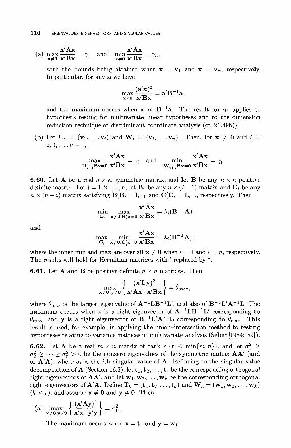
EIGENVALUES. EIGENVECTORS, AND SINGULAR VALUES
- x‘ Ax x‘ Ax
=y1 and min- max ~
X#O x’Bx - yn’ X#O X’BX
with the bounds being attained when x = v1 and x = v,, respectively. In particular, for any a we have
(a‘x) max ~ = a’B-‘a, X#O X’BX
and the maximum occurs when x 0: B-’a. The result for y1 applies to hypothesis testing for multivariate linear hypotheses and to the dimension reduction technique of discriminant coordinate analysis (cf. 21.4913)).
Let Ui = (v1, . . . , vi) and Wi = (vi , . . . ,v,). Then, for x # 0 and i = 2,3 , . . . , n - 1 ,
- x’ Ax x‘ Ax
max ~ = yi and min ~ - 72. U:- B x = O X’Bx WI+,BX=O X’BX
6.60. Let A be a real n x n symmetric matrix, and let B be any n x n positive definite matrix. For i = 1 , 2 , . . . , n, let B, be any n x ( i - 1) matrix and C , be any n x (n - i ) matrix satisfying BiB, = I,-1 and CiC, = I,-,, respectively. Then
x‘ Ax min max ~ = x ~ ( B - ~ A ) B, x#O:B:x=O X’BX
and x’ Ax
max min - - - x~(B-’A), C, ~#O:C:X=O X’BX
where the inner min and max are over all x # 0 when i = 1 and i = n, respectively. The results will hold for Hermitian matrices with ’ replaced by *.
6.61. Let A and B be positive definite n x n matrices. Then
max { ( x ’ L ~ ) 2 } =emax, x # o , ~ # o X’AX . X’BX
where Omax is the largest eigenvalue of A-lLB-’L’, and also of B-’L’A-lL. The maximum occurs when x is a right eigenvector of A-’LB-’L’ corresponding to Omax, and y is a right eigenvector of B-lL’A-lL corresponding to Omax. This result is used, for example, in applying the union-intersection method to testing hypotheses relating to variance matrices in multivariate analysis (Seber [1984: 891).
6.62. Let A be a real m x n matrix of rank T (T 5 min{rn,n}), and let of 2 C T ~ 2 . . . 2 o,” > 0 be the nonzero eigenvalues of the symmetric matrix AA’ (and of A’A), where oi is the ith singular value of A. Referring to the singular value decomposition of A (Section 16.3), let t l , ta, . . . , t, be the corresponding orthogonal right eigenvectors of AA’, and let wl, wg, . . . , w, be the corresponding orthogonal right eigenvectors of A’A. Define T k = (tl, tg, . . . , tk) and wk = (wl, wg,. . . , wk) ( k < T ) , and assume x # 0 and y # 0. Then
max {‘-->=o: x ’ A ~ ) ~ x#O,y#O x’x.y’y
The maximum occurs when x = tl and y = w1.
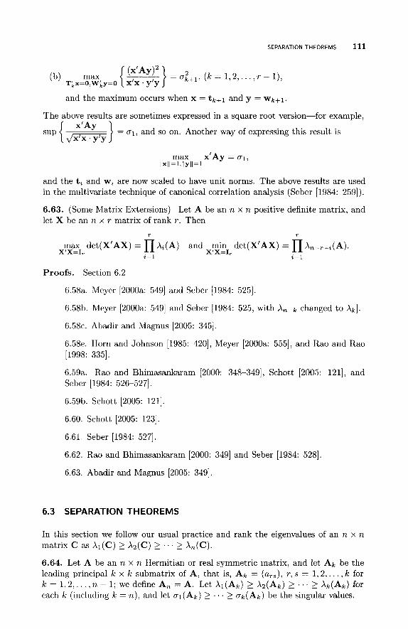
SEPARATION THEOREMS 111
(b) max { M} = (k = 1 ,2 , . . . , T - l), T;x=O,WLy=O X’X . y‘y
and the maximum occurs when x = t k + l and y = wk+l.
The above results are sometimes expressed in a square root version-for example, x‘ A y
= a1, and so on. Another way of expressing this result is sup { d-}
max x’Ay = 01, IIxII=l~llY 11=1
and the ti and wi are now scaled to have unit norms. The above results are used in the multivariate technique of canonical correlation analysis (Seber [1984: 2591).
6.63. (Some Matrix Extensions) Let A be an n x n positive definite matrix, and let X be an n x T matrix of rank T . Then
r r
max det (X’ A X ) = n Xi (A) X’X=I,
i= l
and min det(X’AX) = An-r+i(A). X’X=I,
i= 1
Proofs. Section 6.2
6.58a. Meyer [2000a: 5491 and Seber [1984: 5251.
6.58b. Meyer [2000a: 5491 and Seber [1984: 525, with Xn-k changed to &I.
6 .58~. Abadir and Magnus [2005: 3451.
6.58e. Horn and Johnson [1985: 4201, Meyer [2000a: 5551, and Rao and Rao [1998: 3351.
6.59a. Rao and Bhimasankaram [2000: 348-3491, Schott [2005: 1211, and Seber [1984: 526-5271.
6.5913. Schott [2005: 1211.
6.60. Schott [2005: 1231.
6.61. Seber [1984: 5271.
6.62. Rao and Bhimasankaram [2000: 3491 and Seber [1984: 5281.
6.63. Abadir and Magnus [2005: 3491.
6.3 SEPARATION THEOREMS
In this section we follow our usual practice and rank the eigenvalues of an n x n matrix C as X,(C) 2 X2(C) 2 . . . 2 X,(C).
6.64. Let A be an n x n Hermitian or real symmetric matrix, and let Ak be the leading principal k x k submatrix of A, that is, A k = (ar s ) , T , s = 1,2, . . . , k for k = 1 , 2 , . . . , n - 1 ; w e d e f i n e A , = A . Let XI(&) LX2(Ak) 2 . . . > & ( & ) f o r each k (including k = n), and let al(Ak) 2 . . . 2 a k ( A k ) be the singular values.
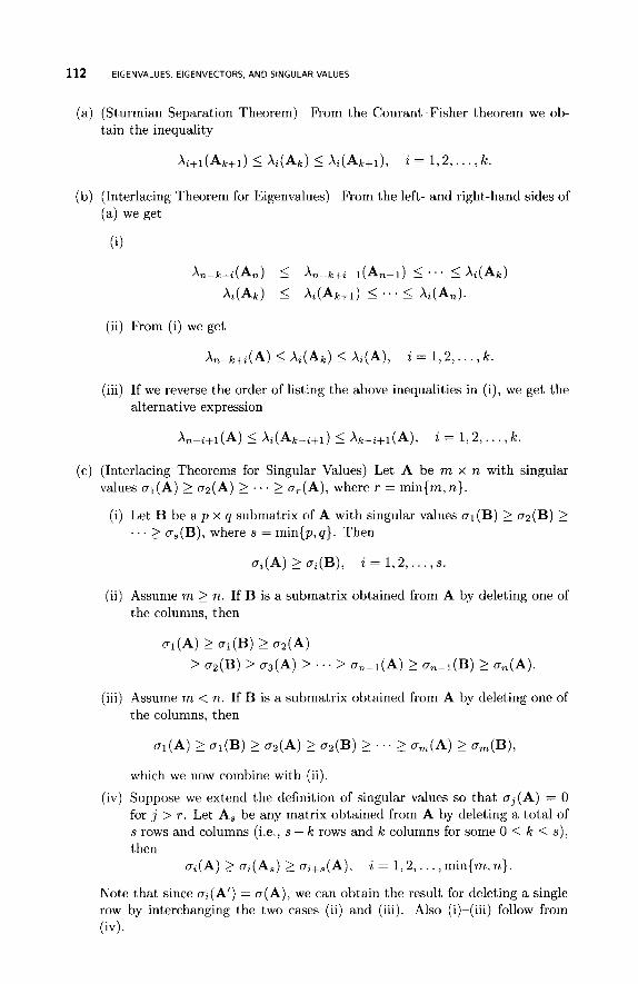
112 EIGENVALUES, EIGENVECTORS. AND SINGULAR VALUES
(a) (Sturmian Separation Theorem) From the Courant-Fisher theorem we ob- tain the inequality
Xi+i(Alc+i) I Xi(&) I Xi(Ak+i), i = 1 , 2 , . . . , k .
(b) (Interlacing Theorem for Eigenvalues) F'rom the left- and right-hand sides of (a) we get
(9
Xn-k+i(An) I Xn-k+z-l(An-l) I . . . I xi(&)
A(&) I X2(Alc+i) I . . . I &(A,).
(ii) From (i) we get
(iii) If we reverse the order of listing the above inequalities in (i), we get the alternative expression
(c) (Interlacing Theorems for Singular Values) Let A be m x n with singular values al(A) 2 Q(A) 2 . . . 2 uT(A), where T = min{m,n}.
(i) Let B be a p x q submatrix of A with singular values al(B) 2 02(B) 2 . . . 2 as(B), where s = min{p,q}. Then
ai(A) 2 a,(B), i = 1 , 2 , . . . , s .
( i i ) Assume m 2 n. If B is a submatrix obtained from A by deleting one of the columns, then
(iii) Assume m < n. If B is a submatrix obtained from A by deleting one of the columns, then
ai(A) 2 ai(B) 2 a2(A) 2 02(B) L . . . L om(A) L am(B),
which we now combine with (ii).
(iv) Suppose we extend the definition of singular values so that aj(A) = 0 for j > T . Let A, be any matrix obtained from A by deleting a total of s rows and columns (i.e., s - k rows and k columns for some 0 I k I s), then
ai(A) a2(A,) 2 O ~ + ~ ( A ) , i = 1,2,. . . ,min{m, n}.
Note that since ai(A') = a(A), we can obtain the result for deleting a single row by interchanging the two cases (ii) and (iii). Also (i)-(iii) follow from (iv).
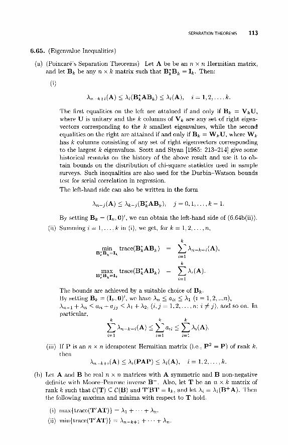
SEPARATION THEOREMS 113
6.65. (Eigenvalue Inequalities)
(a) (Poincark’s Separation Theorems) Let A be be an n x n Hermitian matrix, and let BI, be any n x k matrix such that BiB, = I k . Then:
6)
&-k+i(A) I X2(B;ABk) I &(A), i = 1 ,2 , . . . , k .
The first equalities on the left are attained if and only if B k = vku,
where U is unitary and the k columns of V k are any set of right eigen- vectors corresponding to the k smallest eigenvalues, while the second equalities on the right are attained if and only if BI, = wku, where WI, has k columns consisting of any set of right eigenvectors corresponding to the largest k eigenvalues. Scott and Styan [1985: 213-2141 g’ ive some historical remarks on the history of the above result and use it to ob- tain bounds on the distribution of chi-square statistics used in sample surveys. Such inequalities are also used for the Durbin-Watson bounds test for serial correlation in regression. The left-hand side can also be written in the form
X,-j(A) Xk-j(B;ABk), j = 0 ,1 , . . . , k - 1.
By setting B k = (Ik, 0)’, we can obtain the left-hand side of (6.64b(ii)).
(ii) Summing i = 1,. . . , k in ( i ) , we get, for k = 1 , 2 , . . . ,n,
k
min trace(BiABk) = c X,-k+i(A), B;B,=Ib
i=l
k
The bounds are achieved by a suitable choice of B k .
By setting B k = ( I k , O ) ’ , we have A, I aZ2 5 X,-1 + A, I aZ2 + aJJ I XI + XZ, ( z , ~ = 1 ,2 , . . . , n; z # J ) , and so on. In particular,
(z = 1 , 2 , ... n) ,
k k k
C &-k+t(A) I I C A(A). 2 = 1 2= 1 2= 1
(iii) If P is an n x n idempotent Hermitian matrix (i.e., P2 = P) of rank k , then
X,-k+t(A) I & ( P A P ) I &(A), z = 1 , 2 , . . . , k .
(b) Let A and B be real n x n matrices with A symmetric and B non-negative definite with Moore-Penrose inverse B+ . Also, let T be an n x k matrix of rank k such that C ( T ) C C(B) and T’BT = I k , and let A, = X,(B+A). Then the following maxima and minima with respect to T hold.
(i) max{trace(T’AT)} = X I + . . . + &. (ii) min{trace(T’AT)} = Xn-k+l + . . . + A,.
114 EIGENVALUES. EIGENVECTORS, AND SINGULAR VALUES
(iii) max{tra~e[(T’AT)~]} = A: + . . . + A:.
(iv) min(tra~e[(T’AT)~]} = X:-k+l + . . . + A:. (v) max{trace[(T’AT)-l]} = A;:,+, +. . .+A,1, for A positive definite and
(vi) min{trace[(T’AT)-’]} = A,’ + . . . + X i ’ for A positive definite.
The optimum values are reached when T = (tl, . . . , t k ) , where B1/2ti are or- thonormal right eigenvectors of (B+) ‘I2A(B+) ‘ j 2 associated with the eigen- values X i (i = 1 , 2 , . . . , k ) .
rankB = T .
(c) If A and B are n x n positive definite matrices, then:
(i) X1(ASBS) 5 AT(AB) for 0 5 s 5 1.
(ii) [X1(AB)lt 5 X1(AtBt) for t 2 1
6.66. (Singular Values) Let A be an m x n matrix with singular values ai(A). Let B = U”AV, where U and V are m x p and n x q, respectively, such that U’U = I, and V*V = I,.
(a) If T = (m - p ) + (n - q ) ,
U % + ~ ( A ) 5 ai(B) 5 ai(A), i = 1 , 2 , . . . , min{m,n}.
(b) I f p = q = k ,
I det BI2 = det(BB*) = Xi(BB*) = Ha:(B), i i
so that IdetBI 5 ~ 1 ( A ) . ’ . a k ( A ) .
(c) If p = q = k , we can sum in (a) and obtain, for k = 1 , 2 , . . . ,min{m,n},
k
max I traceB1 = ai(A). u * u = I k ,V’V=I,,
i=l
6.67. Let A be an n x n real symmetric matrix, and let B be an n x n positive definite matrix. If F is any n x k matrix of rank k, then for i = 1 , 2 , . . . , k ,
&[(F’BF)-l(F’AF)] 5 X,(B-lA),
and mFax A, [ (F’BF)-l (F’AF)] = X i (B-’A)
6.68. Let A and B be n x n non-negative definite matrices satisfying C(A) & C(B), and let X be an n x k real matrix with
b = rankB and T = rank(BX)
Then
XbPr+i(B-A) 5 Xi([(X’BX)-X’AX]) 5 Ai(B-A), i = 1 , 2 , . . . ,T.
SEPARATION THEOREMS 115
In the above equation, any choices of the weak inverses B- and (X’BX)- may be made. Equality occurs on the left simultaneously for all i = 1 ,2 , . . . , T if and only if there exists a real n x T matrix QO such that
QbBQo = I,, AQo = BQ&, and C(BQ0) = C(BX).
Here A0 is an T x T diagonal matrix containing the T smallest, not necessarily zero, generalized eigenvalues of A with respect to B.
Equality holds on the right simultaneously for all i = 1 ,2 , . . . , T if and only if there exists a real T x T matrix Q1 such that
QiBQ1 = I,, AQ1 = BQ1A1, and C(BQ1) = C(BX)
Here A1 is an T x T diagonal matrix containing the T largest generalized eigenvalues of A with respect to B . Scott and Styan [1985] give an application to finding distributional bounds on two standard asymptotic hypothesis tests in multiway contingency tables.
6.69. A product version of (6.65a(ii)) is as follows. If A is a Hermitian positive definite matrix and B is an n x k matrix, then
By setting B k = ( I k , O ) ’ and defining Ak as in (6.64), we have
k k
i=l i=l
Proofs. Section 6.3
6.64a. Rao and Bhimasankaram [2000: 347-348, real symmetric case with i and k interchanged; the proof is identical for Hermitian matrices].
6.64b(ii). Rao and Rao [1998: 328, with A,, replaced by B] and Zhang [1999: 222-2251,
6.64b(iii). Schott [2005: 1121.
6.64c(i). Rao and Rao [1998: 3301.
6.64c(ii)-(iii). Horn and Johnson [1985: 4191 and Rao and Rao [1998: 3301.
6.64c(iv). Horn and Johnson [1991: 1491, Rao and Rao [1998: 329-3321, and Zhang [1999: 2291.
6.65a(i). For the real case see Abadir and Magnus [2005: 3471, Schott [2005: 1111, and Rao and Bhimasankaram [2000: 3481.
6.65a(ii). Abadir and Magnus [2005: 348-3491.
116 EIGENVALUES. EIGENVECTORS. AND SINGULAR VALUES
6.65a(iii). Abadir and Magnus [2005: 3481.
6.6513. Quoted by Rao and Rao [1998: 4951.
6 .65~ . Quoted by Rao and Rao [1998: 4951.
6.66a. Rao and Rao [1998: 3381.
6.66b. Horn and Johnson [1991: 1701.
6 .66~ . Horn and Johnson [1991: 1951.
6.67. Schott [2005: 1231.
6.68. Scott and Styan [1985].
6.69. Magnus and Neudecker [1999: 212, real case, with order of eigenvalues reversed] and quoted by Schott [2005: 136, exercise 3.541.
6.4 INEQUALITIES FOR MATRIX SUMS
6.70. (Eigenvalues) Let A and B be n x n Hermitian or real symmetric matrices, and let C = A + B, with corresponding eigenvalues
a1 2 a 2 2 . . . 2 an; Pi 2 P 2 2 . . . 2 Pn and 71 2 7 2 . . . 2 T n ,
respectively. Then:
(a)
a 2 + Pn a3 + Pn-1
an+ P2
. . . L 7 2 2 a 2 + P1
INEQUALITIES FOR MATRIX SUMS 117
(b) It follows from (a) that
yi I ag +P2--3+i , for j = 1 ,2 , . . . ,i; i = l , ~ , . . . ,n ,
and yi 2 aj + Pn-j+i, for j = i , i + 1,. . . ,n; i = 1,2, . . . , n.
(c) (Weyl's Theorem) From (b) we have:
(i) For i , j I n
Xi(A+B) 5 Xj(A) +Xi-j+l(B) for j 5 i, &(A + B) 2 Xj(A) + An+i-j(B) for j 2 i.
(ii) If in (i) we make the subscript substitution j = a and i - j + 1 = b so that i = a + b - 1, and then relabel, we get from the first equation
Xa+b-l(A + B) I ,&(A) + X b ( B ) , a + b - I 5 71, b 2 1.
(iii) Setting j = i in (i) we have, for i = 1 ,2 , . . . , n,
&(A) + L ( B ) I &(A + B) I &(A) + Xi(B).
(iv) (Monotonicity of Eigenvalues) If B is real non-negative definite and A is real symmetric, then X2(B) 2 0 for all i and, from (iii),
X2(A) 5 &(A + B) , i = 1 , 2 , . . . ,n.
If B is positive definite, then the inequality is strict.
(i) (Lidski;) Let Z l , z 2 , . . . , i k be integers satisfying 1 5 (d) < . . . < i k I n. Then for k = 1 ,2 , . . . , n,
j=1 j=1 j=1
(ii) (Sum of the k largest eigenvalues) For k = 1 ,2 , . . . , n,
k k k k
(e) Suppose B is a real symmetric matrix with rankB 5 T and A is real sym- metric. For i = 1,2, . . . , n - T we have:
6.71. (Convexity) For any two real symmetric n x n matrices A and B, and O I c r 5 1 ,
Xi[aA + (1 - a)B] Xn[aA + (1 - a)B]
I 2
aXi(A) + (1 - a)Xi(B), aXn(A) + (1 - a)An(B).
118 EIGENVALUES, EIGENVECTORS. AND SINGULAR VALUES
Hence, A1 is convex and A, is concave on the space of real symmetric matrices. Putting a = 1/2 gives us
Al(A + B) I Al(A) + Al(B), &(A + B) 2 &(A) + A,(B).
6.72. (Singular Values) Let A and B be m x n matrices, and let p = min{m,n}. Then:
(4 ai(A + B) 5 o.j(A) + oi-j+l(B), j = 1,2, . . . ,i; i = 1,2, . . . ,p .
~ i + j - l ( A + B) I oi(A) + oj(B), 1 I i , j I p ; i + j I p + 1.
(b) In particular,
(i) 01 (A + B ) I o1 (A) + o1 (B). (ii) op(A + B) I min{op(A) + ol(B),ol(A) + op(B)}.
(iii) oi(A) + on(B) I oi(A + B) I oi(A) + ol(B).
(c) Ioi(A + B) - oi(A)I 5 ol(B) for i = 1 , 2 , . . . , p .
i=l i= 1
Proofs. Section 6.4
6.70a. Rao and Rao [1998: 3221.
6.70c(i). Bhatia [1997: 62, with i and j interchanged].
6.7Oc(ii). Schott [2005: 114, real case].
6.7Oc(iii). Schott [2005: 112, real case] and Zhang [1999: 2271.
6.7Oc(iv). Magnus and Neudecker [1999: 208-2091 and Schott [2005: 119- 1201.
6.70d(i). Wielandt [1955] and Diimbgen [1995].
6.70d(ii). Schott [2005: 115-1161.
6.70e. Schott [2005: 112-1141.
6.71. Abadir and Magnus [2005: 344-3451 and Magnus and Neudecker [1999: 205, A1 and A, are interchanged].
6.72a. Rao and Rao [1998: 326-327, 3601 and Horn and Johnson [1991: 178, subscripts reordered].
6.72b(iii). Zhang [1999: 2281.
6 .72~. Horn and Johnson [1991: 1781.
6.72d. Horn and Johnson [1991: 1961.
INEQUALITIES FOR MATRIX DIFFERENCES 119
6.5 INEQUALITIES FOR MATRIX DIFFERENCES
6.73. Let A, B, and A - B be Hermitian non-negative definite n x n matrices with rankB 5 k . Then
&(A - B) 2 Xk+z(A)
for all i ( k + i 5 n) with equality for all i if and only if
i= 1
where ul, u2,. . . , uk are the first k orthonormal eigenvectors of A (i.e., those cor- responding to the Xi(A), i = 1 , 2 , . . . , k ) .
6.74. Let A and B be m x n matrices with ranks r and s, respectively. Then:
ai (A-B) L O ~ + ~ ( A ) , i + s I r , 2 0, i + s > r .
(b) The equalities in (a) are attained if and only if s 5 r and
where the singular value decomposition of A is A = EL==, ai(A)uiuf.
Proofs. Section 6.5
6.73. Quoted by Rao and Rao [1998: 3821, though the proof is similar to that of (6.74).
6.74. Rao [1980: 8-91,
6.6 INEQUALITIES FOR MATRIX PRODUCTS
6.75. Let A be an n x n non-negative definite matrix, and let B be an n x n positive definite matrix. If i, j , k = 1,2, . . . , n such that j + k 5 i + 1, then:
(a) Xz(AB) 5 Xj(A)Xk(B).
(b) X,-z+i(AB) 2 Xn-j+l(A)Xn-k+l(B)
The case when A is symmetric and B is non-negative definite is discussed in detail by Makelainen [ 19701.
6.76. If A and B are n x n Hermitian non-negative definite matrices, then
X,(A)X,(B) 5 X,(AB) 5 X,(A)Xl(B), i = 1,2 , . . . ,n.
120 EIGENVALUES. EIGENVECTORS. AND SINGULAR VALUES
6.77. (von Neumann) (Trace) If A and B are n x n Hermitian matrices, then
n n
Xi(A)Xn-i+l(B) 5 trace(AB) 5 cXi(A)Xi(B). i= 1 i=l
Equality holds on the right when B = Cr=l Xi(B)uiuf, and equality holds on the left when B = Cyzl X,-i+l(B)uiuf. Here ui is a right eigenvector of A for the eigenvalue Xi(A), i = 1 , 2 , . . . , n.
6.78. Let A and B be n x n non-negative definite matrices. If 1 5 il < . . . < ik then
n,
k k
with equality for k = n.
6.79. (Partial Sum) Let A and B be n x n (real) non-negative definite matrices. Then
I;. Ic c Xi(A)Xn-i+l(B) 5 c Xi(AB), k = 1 , 2 , . . . , n. i = l i= 1
6.80. Let A be an m x n and B an n x m real or complex matrices. Then
ai(A)a,(B) 5 ai(AB) 5 ai(A)ol(B), i = 1 , 2 , . . . , m
6.81. Let A be an m x n and B an n x m real or complex matrices, and let p = min{m, n}. Then, for singular values a(.),
P P
- x o a ( A ) ~ i ( B ) 5 trace(AB) 5 x ~ i ( A ) a i ( B ) .
Equality holds on the right when B = CE1ai(B)qipf, and equality on the left holds when B = Cr=’=, oi(B)(-qi)pf, where pi and qi are the singular vectors of A for ai(A), i = 1 , 2 , . . . , p (cf. Section 16.3).
6.82. (Horn) Let A be an m x p and B an p x n real or complex matrices, and let q = min{ m, n, p } .
i= 1 i=l
i a
(a) n C ~ ( A B ) 5 IT a j ( ~ ) a j ( ~ ) , i = I, 2 , . . . , q . j = 1 j=1
If A and B are square matrices of the same order (i.e., m = n = p ) , then equality holds in the above equation for i = n.
(b) C:=l[aj(AB)]P 5 C:=l[oj(A)aj(B)]P for i = 1 , 2 , . . . , q and any p > 0.
Horn and Johnson [1991: 1771 give some extensions to functions of the singu- lar values.
INEQUALITIES FOR MATRIX PRODUCTS 121
6.83. Let A and B be real n x n symmetric matrices, and let T be an n x n orthogonal matrix. Then
n
maxtrace(TAT'B) = c Xi(A)Xi(B) and T i=l
n
min trace(TAT'B) = c Ai(A)An+l-i(B). T
2= 1
Setting
we have E
max trace(R'AR) = &(A). R'R=Ik
i=l
6.84. Let Xi be an n x pi matrix of rank pi (i = 1,2) . Then the eigenvalues of (X~Xz)-'X~Xl(X:X,)-'X:X, are less than or equal to one. This result arises in the correspondence analysis of a contingency table.
6.85. If A and B are n x n real or complex matrices of which at least one is nonsingular, then
Xmin (AA*)Xrnin (BB*) I Xi (AB)Xi (AB) I Xmax(AA* )Amax (BB*)
for all i. If A and B are both Hermitian, one is positive definite (say A), and the other is non-negative definite, then
Xrnin(A)Xrnin(B) I Xi(AB) I Anax(A)Anax(B).
Proofs. Section 6.6
6.75. Schott [2005: 126-1271,
6.76. Zhang [1999: 2271.
6.77. Rao and Rao [1998: 3861.
6.78. Lidski; [1950] and quoted by Schott [2005: 1271.
6.79. Quoted by Schott [2005: 128; see also 137, exercise 3.571.
6.80. Zhang [1999: 2281.
6.81. Rao and Rao [1998: 3871.
6.82a. Horn and Johnson [1991: 1721 and Rao and Rao [1998: 340-3421.
6.82b. Horn and Johnson [1991: 1771.
6.83. Anderson [2003: 6451.
6.84. B6nassBni [2002].
6.85. Roy [1954].
122 EIGENVALUES, EIGENVECTORS. AND SINGULAR VALUES
6.7 ANTIEIGENVALUES AND ANTIEIGENVECTORS
If A is an n x n positive definite matrix, then the cosine of the angle 0 between n x 1 real vectors x and Ax is (cf. Definition 2.12 in Section 2.2.1)
x‘ Ax
~ ( X ’ X ) (x’A2x) ’ coso =
which has the value of unity when x is an eigenvalue of A, that is Ax = Ax for some A. This raises the question of what value of x minimizes cos 8, or equivalently maximises the angle beween x and Ax. This question motivates the following definitions.
Definition 6.7. Let A1 2 A:! 2 . . . 2 A, > 0 be the eigenvalues of positive definite A and X I , x2, . . . , x, be the corresponding right eigenvectors. Referring to the above introduction, cos 0 takes its minimum value of
by the Kantorovich inequality (12.2a) (with x = A1/2y), and the minimum is attained at
= (u1, uz), say. 6 x 1 * JGxn
&FK X=
The vectors (u1, ug) are called the first antieigenvectors and 1-11 value. The angle 0 is called the angle of the operator of A. We
P2 = min x’ Ax
x l x i , ~ , J(x’x)(x’A2x)
the first antieigen- then define
which is attained at
We call 1-12 the second antieigenvalue of A and (us, ud) the second antieigenvectors. We then find the third set by minimizing cos0 subject to x I {x l ,x~ ,xn- l ,xn} , and carry on this process until we have 1-11 5 1-12 5 . . . 5 pLT ( r = [p/2]), where
are the ordered antieigenvalues and (u1, uz), (us, uq), . . . (uzr-1, uzr) are the cor- responding pairs of antieigenvectors. When p is odd, the antieigenvalue of order (n + 1)/2 is unity, with the corresponding antieigenvector X ( ~ + ~ ) / Z .
The above terminology and concepts were introduced by Gustafson [1968] under the umbrella of operator trigonometry. The theory was extended to arbitrary non- singular matrices by Gustafson [2000]. He also applied the theory to the question
ANTIEIGENVALUES AND ANTIEIGENVECTORS 123
of one measure of efficiency of the ordinary least squares estimator (OLSE) with respect to the best linear unbiased estimator (BLUE) in Gustafson [2002, 20051. Rao [2005] also discussed this question in detail.
6.86. If A is an n x n positive definite matrix, then
A2x 2Ax x’A2x ~ ‘ A X
+ x = o
is called the Euler Equation. This equation is satisfied by all the eigenvectors xi of A, and the only other solutions are the antieigenvectors
This topic has links with canonical correlations (Gustafson [2005: 1161).
6.87. Let A be a positive definite n x n matrix. Then
max [x’Ax - (x’A-lx)-’] = (A - x‘x=l
with the maximum occurring at
x = ( 6 )1’2xl* ( 6 )’”.,, 6+6 dx+K
where x1 and x, are the eigenvectors corresponding to A1 and A,, the maximum and minimum eigenvalues of A. Rao [2005: 64-65] uses the above result t o define the first of another series of antieigenvalues that he calls the SM-antieigenvalues, with corresponding antieigenvectors.
Proofs. Section 6.7
6.86. Gustafson [2002, 20051.
6.87. Shisha and Mond [1967] and Styan [1983].

This Page Intentionally Left Blank
CHAPTER 7
GENERALIZED INVERSES
When a matrix is not square, or square and singular, then an inverse does not exist. However, a type of inverse does exist for these matrices called a generalized inverse that functions very much like an inverse. Such inverses are very useful in statistics for finding explicit solutions for a variety of problems such as the solution of linear equations so that this chapter has close links with Chapter 13. The reader should also consult Chapter 14 on partitioned matrices. A summary of some computational aspects of generalized inverses, along with references, is given by Ben-Israel and Greville [2003: chapter 71.
7.1 DEFINITIONS
Definition 7.1. A weak inverse of an m x n matrix A is defined to be any n x m matrix G that satisfies the condition
(1) AGA = A.
Such a matrix always exists (by 7.1 below), but it is not unique. We shall write G = A- . Many of the results below are proved by verifying] or finding conditions, that (1) is true.
Note that the name “generalized inverse” is fairly common but not universal. Other terms used include conditional inverse (cf. Graybill [1983: chapter 6]), pseu- doinverse, g-inverse, and weak inverse. I shall use the term weak inverse to avoid confusion.
A Matmx Handbook for Statzstzcaans. By George A. F. Seber Copyright @ 2008 John Wiley & Sons, Inc.
125
126 GENERALIZED INVERSES
If A is real and G also satisfies
(2) GAG = A,
(3) AG is symmetric,
(4) GA is symmetric,
then we call G the Moore-Penrose inverse and write G = A+. The above definition applies to complex matrices A if we replace “symmetric” by “Hermitian.”
There are other matrices G that satisfy just one or more of the above four conditions, and we shall use subcripts to identify the conditions. For example, if G satisfies at least (1) and (2) we shall call G a glz-inverse and write G = A-
(12). Similarly we can write A- = A;) and refer to A- as a gl-inverse. We shall only use the subscript notation if there is any danger of ambiguity. For one list of the various inverses see Rao and Rao [1998: 2941.
We shall also define A{z, j , . . . , p } to be the set of all matrices G which satisfy at least the conditions (i), (j), . . . , (p) . Thus A&) E A{1,2}, A- E A{1}, and so on. We shall discuss these inverses later.
If A is square, then a generalized inverse G that satisfies (l), (2), and AG = GA is called the group inverse, which we denote by A#.
7.2 WEAK INVERSES
7.2.1 General Properties
Let A be an m x n real or complex matrix of rank r. Many of the following results can be proved by simply checking that condition (1) above holds.
7.1. (Existence) From (16.33) there exist conformable nonsingular matrices B and C such that
Then A- = C ( ) B for arbitrary X , Y , and Z of appropriate sizes. Al-
though a weak inverse always exists, we see that it is not unique. Another version based on the singular value decomposition is given in (7.82).
7.2. (Basic Properties)
(a) Taking the transpose of both sides of AA-A = A, we see that A-‘ is a weak inverse of A’. Although we shall write (A-)’ = (A’)-, what we mean, technically, is that A-’ E A’{l}. This idea underlies all the results below.
(b) For k # 0, kklA- is a weak inverse kA.
(c) A-A and AA- are each idempotent. Also, since Pc(A) = AA- is not generally symmetric, it represents a nonorthogonal (oblique) projection onto C(A). Similarly, Pc(A,) = (A-A)’ = A’A’- represents an oblique projection onto C(A’).
WEAK INVERSES 127
(d) rank(AA-) = trace(AA-) = trace(A-A) = rank(A-A) = rankA _< rank(A-).
(e) C(AA-) = C(A), N ( A A - ) = N ( A ) , and C[(A-A)*] = C(A*).
( f ) Taking conjugate transposes of AA-A = A we get (A*)- = (Ap)*.
(8) rankA = m if and only if AA- = I, (i.e., A- is a right inverse of A) .
(h) rankA = n if and only if A - A = I, (i.e., A- is a left inverse of A).
(i) A(A*A)-A*A = A and A*A(A*A)-A* = A*. This means that (A*A)-A* is a weak inverse of A, and A(A*A)- is a weak inverse of A*.
(j) A(A*A)-A* is Hermitian, idempotent, and invariant for any choice of the weak inverse (A*A)-.
(k) A * A G A = A*A if and only if G is a weak inverse of A .
7.3. The following conditions are equivalent.
(1) G is a weak inverse of A.
(2) A G is idempotent and rank(AG) = rank A.
(3) G A is idempotent and rank(GA) = rank A.
(4) rank(1, - G A ) = n - rankA.
7.4. (Symmetric and Hermitian Matrices)
(a) A Hermitian matrix has a Hermitian weak inverse, namely ;(A- + (A-)*).
(b) A Hermitian matrix A has a non-negative definite weak inverse if and only if A is non-negative definite.
7.5. (Rank of Inverse)
(a) Taking X = 0 and Y = 0 in (7.1) and noting that the rank is unchanged by multiplying by a nonsingular matrix, we see that
rank(A-) = rank A + rank Z.
Since Z is arbitrary, there exists an A- having any specified rank between rankA and min{m,n} (Rao and Mitra [1971: 311). In particular, we can choose Z such that A- has full row or column rank (i.e., the rows or columns are linearly independent).
(b) rank(A-) = rankA if and only if A- is also a gl,z-inverse
7.6. (Representation of A{ 1)) Let A- be any weak inverse of A. Then we have the following representations.
(a) (i) A{ 1) = {X : X = A- + H - A-AHAA- ; H arbitrary}.
(ii) A{ 1) = {X : X = A- + ( I - A - A ) F + G(I - AA-) ; F, G arbitrary}.
128 GENERALIZED INVERSES
(b) Let A,, A,, and A3 be any (not necessarily the same) fixed weak inverses of A. Then B1 and B2 are also weak inverses of A , where
B1 = A,+F-A,AFAA,,
Bz = A, + (I - A,A)F + G(I - AA,).
Here F and G are abitrary matrices of appropriate sizes. Also, any weak inverse of A can be written as B1 and as B2 for some matrices F and G.
If we consider the special case of A,, A,, and A3 being all the same, we see that B1 and B2 reduce to (a)(i) and (a)(ii), respectively.
(c) If A and B are m x n matrices with A{ 1) = B{ l}, that is every weak inverse of of A is a weak inverse of B, and vice-versa, then A = B.
7.7. (Rank and Products)
(a) rank(ABC) = rankB implies that C(ABC)-A is a weak inverse of B. We can set A = I or C = I.
(b) Let V be a matrix such that rank(A*VA) = rankA (which is automatically satisfied if A is Hermitian positive definite), then:
(i) A(A*VA)-(A'VA) = A and (A*VA)(A*VA)-A* = A*.
(ii) A(A*VA)-A* is invariant for any choice of (A*VA)- and is of the same rank as A. If A'VA is Hermitian, then so is A(A*VA)-A*.
7.8. If A is m x n and D is m x m, and both are of rank m, then
D-' = A(A'DA)-A'.
7.9. (Hermite Form)
(a) If A is n x n and B is nonsingular such that BA = HA, where HA is in Hermite form (Section 16.2.4), then B is weak inverse of A.
(b) Let A be an m x n (m > n) matrix, and let A0 = (A,Omx(,,-n)). Let €30 be a nonsingular matrix such that BoAo = H, where H is in Hermite form. Suppose Bo is partitioned as
Bo = ( BBl) where B is n x m. Then B is a weak inverse of A. A similar result holds for m < n.
7.10. Let A and B be m x n complex matrices. Then the following statements are equivalent:
(1) The nonzero eigenvalues of B - A are invariant with respect to B-.
(2) trace(B-A) is invariant with respect to B-.
(3) C(A) C(B) and C(A*) C C(B*).
WEAK INVERSES 129
Proofs. Section 7.2.1.
7.1. Ben-Israel and Greville [2003: 411 and Graybill [1983: 1361.
7.2b. The result follows from the definition of a weak inverse.
7 . 2 ~ . A-AA-A = A - A and AA-AA- = AA- . Also P ~ ( A ~ A = A and then take the transpose of AP&,,) = A .
7.2d. Graybill [1983: 1341, Rao and Bhimasnakaram [2000: 1951, and Schott [2005: 203-2041.
7.2e. Ben-Israel and Greville [2003: 431
7.2g-7.2h. Ben-Israel and Greville [2003: 431 and Schott [2005: 2041
7.2i. Rao [1973a: 261 and Rao and Mitra [1971: 221.
7.2j. Rao [1973a: 261 and Rao and Rao [1998: 268-2691
7.2k. Rao and Mitra [1971: 221.
7.3. Rao and Bhimasankaram [2000: 195, (1)-(3)] and Rao and Mitra [1971: 21, 231.
7.4b. Arguing as in (7.21) for Hermitian matrices, we have A = UAU*, where U is unitary and A is a diagonal matrix of non-negative eigenvalues. We then set A- = UA-U*, which is Hermitian non-negative definite.
7.5b. Rao and Mitra [1971: 281.
7.6a(i). Rao and Mitra [1971: 261 and Schott [2005: 2041.
7.6a(ii). Rao and Mitra [1971: 261.
7.6b. Graybill [1983: 1371
7 .6~ . Rao and Mitra [1971: 271 and Rao and Rao [1998: 2771.
7.7a. Rao and Mitra [1971: 221 and Schott [2005: 2051.
7.7b. Rao and Mitra [1971: 221.
7.8. This follows from (7.7a) by noting that rank(A’DA) = rankD, since D is nonsingular.
7.9. Graybill [1983: 1321.
7.10. Baksalary and Puntanen [1990].
130 GENERALIZED INVERSES
7.2.2 Products of Matrices
7.11. (Invariance Properties)
(a) The matrix BA-C is invariant for any choice of A- if and only if C(B‘) c C(A’) and C(C) g C(A).
(b) From (a), If A is a real symmetric matrix, then B’A-B is invariant for any choice of A- if and only if C(B) C(A).
(c) F’rom (a), if A is any n x n matrix with c & C(A) and c C C(A’), then c’A-c is invariant with respect to A-.
(d) (Regression) Let X be any real matrix and let G = (X’X)- be any weak inverse of X’X.
(i) If c c C(X’), then c’(X’X)-X’ is invariant for any weak inverse of X’X.
(ii) X(X’X)-X’ = XX+ is invariant and symmetric, being the orthogonal projector onto C(X). Here X+ is the Moore-Penrose inverse of X.
(iii) G’ is also a weak inverse of X’X.
(iv) (X’X)-X’ is a weak inverse of X.
(e) If rank(CAB) = rankC = rankB, then B(CAB)-C is invariant for any choice of (CAB)-.
7.12. If P is idempotent, then P ( P A P ) - P is a weak inverse of PAP.
7.13. Noting that FF- and (F-F)’ = F’F’-, being idempotent, represent (oblique) projections onto F and F’, respectively (cf. 7.2c), we have the following for con- formable matrices.
(a) BA-A = B if and only if C(B’) C(A‘), that is, if and only if there exists a matrix D such that B = DA.
(b) AA-B = B if and only if C(B) C(A), that is, if and only if there exists a matrix D such that B = AD.
(c) (CAB)(CAB)-C = C if and only if rank(CAB) = rankC.
(d) B(CAB)-(CAB) = B if and only if rank(CAB) = rankB.
7.14. Let A be an m x n matrix, B be an rn x m matrix, and C be an n x n matrix.
(a) If B and C are nonsingular, (BAC)- = C-lA-B-’ for some weak inverse A- of A.
(b) If A has rank m and B is nonsingular, then (A’BA)- = A-B-lA’-.
(c) (AB)- = B-A- if and only if P = A-ABB- is idempotent
7.15. Let A, B, and C be m x n, p x m, and n x q matrices, respectively. If B has full column rank m, and C has full row rank n, then
(BAC)- = C-A-B-.
WEAK INVERSES 131
We can also get special cases by setting one of the matrices equal to the identity matrix.
7.16. If (A’A)- is a weak inverse of A’A, then so is (A’A)-’.
7.17. The following hold for weak inverses A- and B-.
(a) (I - AA-)B-BA = -(I - AA-)(I - B-B)A.
(b) BAA-(I - B-B) = -B(I - AA-)(I - B-B).
(c) (BA)- = A-B- - A-(I - B-B)[(I - AA-)(I - B-B)]-(I - AA-)B-.
(d) Let A be an m x n matrix and B be an n x p matrix. If rankB = n, then (AB)- = B-A-.
(e) C(A) n C(B) = 0 if and only if (AA’ + BB‘)- is a weak inverse of AA’.
Proofs. Section 7.2.2.
7.11a. Graybill [1983: 134-135, with the notation change A“ + A- and A- + A+] and Rao and Mitra [1971: 211. An alternative proof using the idea of extremal ranks is given by Tian [2006a: 951. He also gives necessary and sufficient conditions for rank(BA-C) to be invariant with respect to A-.
7.11d(i). Graybill [1983: 1351.
7.1 Id( ii)-( iv) . Searle [ 1982: 22 1-2221.
7.11e. Rao and Mitra [1971: 221.
7.12. Follows from the definition of a weak inverse.
7.13a-b. Schott [2005: 2051 and Rao and Mitra [1971: 21-22]
7.13~-d. Harville [2001: 106, exercise 441.
7.14a. Harville [1997: 113, lemma 9.2.41.
7.14b. From (7.2g) we have AA- = I,, and then use the definition of weak inverse.
7 .14~. Harville [2001: 51, exercise 81. If P2 = P, then AP2B = APB, which implies that (AB)- = B-A-. The converse is straightforward.
7.15. We use the fact that B-B = I, and CC- = I, from (7.2g) and (7.2h).
7.16. Schott [2005: 206-2071.
7.17. Isotalo et al. [2005b: chapter 121 and (a)-(c) quoted by Searle [1982: 2261. For (d) we have AB(B-A-)AB = AB since BB- = I,.
132 GENERALIZED INVERSES
7.2.3
7.18. The following conditions are equivalent for any weak inverse (A + B)-.
Sums and Differences of Matrices
(2) (A + B)- is a weak inverse of both A and B.
(3) C(A) n C(B) = 0 and C(A’) n C(B’) = 0.
7.19. Let A, B, C, and V be real conformable matrices with V positive definite, and C(C) = C(A’) nC(B). Let QB = I - PB, where PB = B(B’B)-B’.
A( A‘VA) - A‘ - AQB ( QB A‘VAQB ) - QB A’ = A( A’VA)-C [C’( A’VA)- C] - C’( A’VA)-A’.
(b) V-’ - QB(QBVQB)-QB = V-lB(B’V-lB)-B’V-l
QB can be replaced by a matrix with the same range. The above results are used in the theory of singular linear regression models.
Definition 7.2. Given A and B both m x n matrices, then A(A + B)-B is called the parallel sum of A and B. Some authors call (A+ + B+)+ the parallel sum and, under certain conditions, the two definitions are equivalent. For properties relating to both definitions and their equivalence, see Rao and Mitra [1971: 186-1921. They also define a parallel difference.
7.20. For conformable matrices
(a) AA’(AA’ + BB’)-BB’ = BB’(AA’ + BB’)-AA’.
(b) [AA’(AA’ + BB’)-BB’]- = (AA’)- + (BB’)-
Proofs. Section 7.2.3.
7.18. Harville [1997: 4211. We obtain (2) by multipying out (1) to get A(A+ B)-A = A, B(A + B)-B = B, A(A + B)-B, and B(A + B)-A.
7.19-7.20. Kollo and van Rosen [2005: 501.
7.2.4 Real Symmetric Matrices
Let A be a real symmetric matrix.
7.21. By (16.44) there exists orthogonal T such that
where A, is a nonsingular r x r diagonal matrix consisting of the nonzero eigenvalues of A. Then
WEAK INVERSES 133
where X, Y , and Z are arbitrary. Note that A- need not be symmetric. (When A is Hermitian, then T is unitary and T' is replaced by T*.)
7.22. Suppose A is n x n, P is symmetric and idempotent, A + CP is nonsingular, and PA = 0.
(a) (A + cP)-' is a weak inverse of both A and P.
(b) In particular, if Al, = 0, J, = 1,l; (=nP), and A + dJ, is nonsingular, then (A + dJ,)-' is a weak inverse of A. Furthermore,
A+ = (A + dJ,)-' - (dn2)-lJ,.
These results are useful in experimental designs (e.g., John and Williams [1995: 231).
7.23. Suppose that 1 + 1 # 0 in the underlying field F. Since (A-)' is a weak inverse of A', a symmetric weak inverse of a symmetric matrix A always exists, namely B = ;[A- + (A-)'I.
7.24. From the definition of a weak inverse, if A and A-A are symmetric, then (A-)2 is a weak inverse of A2.
Proofs. Section 7.2.4.
7.21. Searle [1982: 2201.
7.22. John and Williams [1995: 231
7.23. Since A-' = A'- = A-. we have AA-'A = A and B = A-.
7.2.5 Decomposition Methods
7.25. (Diagonalizable Matrices) If A is diagonalizable of rank T , we have from (16.17) the spectral decomposition A = cr=l X,F, = c:='=, X,F,, where A"=,+' = . f . = A, = 0. Then:
(a) c;==, XL'F, is a weak inverse of A.
(b) (A + C:="=,+, azF,)-l is a weak inverse of A for all nonzero real a,+l,. . . ,a,.
7.26. There exist permutation matrices II1 and II, such that
where B11 is a nonsingular T x T matrix and T = rank A. Then A = IIiBIIL and
BT: 0 B - = ( 0 0 )
is a weak inverse of B. Also IIzB-IIl is a weak inverse of A.
Proofs. Section 7.2.5.
7.25. Hunter [1983a: 1501.
7.26. Searle [1982: 217-2181.
134 GENERALIZED INVERSES
7.3 OTHER INVERSES
In this section we assume real matrices. However, many of the results hold for complex matrices by simply replacing ’ by *.
7.3.1 Reflexive (912) Inverse
Let A be an m x n matrix and G an n x m matrix. As noted at the beginning of this chapter, G = AT2 is a 912-inverse of A if AGA = A and GAG = G, i.e., if G is a weak inverse of A and A is a weak inverse of G. Such an inverse is usually refered to as a reflexive generalized inverse or reflexive g-inverse.
7.27. If A is m x n, we have from (3.5) the full-rank factorization A = CmX,RTXn, where C and R have rank r. Let D and S be the left and right inverses of C and R, respectively, so that DC = I, and RS = I,. Then SD is a reflexive g-inverse of A.
7.28. If A; and A, are any (possibly different) weak inverses of A, then ATAA, is a gl2-inverse of A.
7.29. Every reflexive g-inverse of a matrix A can be expressed in the form of A-AA- for some weak inverse A- of A.
7.30. A weak inverse G of A is a gl2-inverse if and only if r ankG = rank A.
7.31. If G is a gl2-inverse of A, then G’ is a gl2-inverse of A’.
7.32. (Invariance) If A, B, and C are nonzero conformable matrices, then AB,C is invariant with respect to BL2 if and only if C(A’) C C(B’) and C(C) 2 C(B).
Proofs. Section 7.3.1.
7.27. Rao and Rao [1998: 2791.
7.28. Harville [1997: 496, lemma 20.3.21
7.29. Rao and Mitra [1971: 281.
7.30. Harville [1997: 4971 and Rao and Rao [1998: 2791.
7.31. Harville [1997: 4971.
7.32. Tian [2006a: 1001 proved this using his extremal rank technique. He also gave necessary and sufficient conditions for the rank to be invariant.
7.3.2 Minimum Norm (914) Inverse
The matrix G is a 914-inverse of A if AGA = A and GA is symmetric (or Hermi- tian if A is complex). It is usually refered to as a minimum norm g-inverse.
7.33. The following conditions are equivalent.
(1) G is a 914-inverse of A.
OTHER INVERSES 135
(2) GAA’ = A’.
(3) AA’G = A.
(4) GA = Pc(A,), where Pc(A,), being symmetric and idempotent, represents the orthogonal projection onto C(A’). (In this case GA is invariant to the choice of G.)
In the complex case we replace ’ by *.
7.34. If G is a gl4-inverse, then x = Gy minimizes llxll2 subject to Ax = y .
7.35. A{14} = {G : G = AC4 + Z(1, - AA,)), where Z is an arbitrary n x m matrix.
7.36. (Product Invariance) If A, B, and C are nonzero conformable matrices, then AB,C is invariant with respect to BC4 if and only if C(C) C C(B).
Proofs. Section 7.3.2.
7.33. Harville [1997: 498-4991.
7.34. Harville [1997: 497, theorem 20.3.61 and Rao and Rao [1998: 2881.
7.35. Ben-Israel and Greville [2003: 551.
7.36. Tian [2000a: 1051.
7.3.3
Let A be an m x n matrix and G an n x m matrix. As noted at the beginning of this chapter, G is a gl24-inverse of A if AGA = A, GAG = G and GA is symmetric. Since it combines a g12 and a ~ 1 4 inverse, it is refered to as a minimum n o r m reflexive g-inverse.
7.37. A matrix G is a glzd-inverse of A if and only if G = A’(AA’)- for some weak inverse (AA’)- of AA’.
7.38. If G is a glzd-inverse of A, then C(G) = C(A’).
7.39. A(124) = {G : G = AT24 + AT24Z(11L - AA,,)}, where Z is an arbitrary n x m matrix.
Minimum Norm Reflexive (9124) Inverse
Proofs. Section 7.3.3.
7.37-7.38. Harville [ 1997: 4991.
7.39. Quoted by Ben-Israel and Greville [2003: 561.
136 GENERALIZED INVERSES
7.3.4 Least Squares (913) Inverse
Let A be an m x n matrix and G an n x m matrix. As noted at the beginning of this chapter, G is a gl3-inverse of A if AGA = A and AG is symmetric. It is usually refered to as a least squares g-inverse and is denoted by AT3. In what follows, we can replace ’ by * in the complex case.
7.40. A p x n matrix G is a gl3-inverse of the n x p matrix X if and only if (y - Xb)’(y - Xb) is minimized at b = Gy.
7.41. The following statements are equivalent.
(1) A matrix G is a gl3-inverse of A.
(2) A‘AG = A’ or, equivalently, G’A’A = A.
(3) AG = Pc(A), where Pc(A) = A(A’A)-A’ represents the orthogonal projec- tion onto C(A).
7.42. Let G be a gl3-inverse of A. Then:
(a) AG is invariant to the choice of G.
(b) C(G‘A‘) = C(A).
7.43. (A’A)-A’ is a g13-inverse of A for any weak inverse, (A’A)-, of A’A.
7.44. A(13) = {G : G = AT3 + (I, - AF3A)Z},
where Z is an arbitrary n x m matrix.
7.45. (Product Invariance) then AB,C is invariant with respect to BF3 if and only if C(A’) C C(B’).
If A, B, and C are nonzero conformable matrices,
Proofs. Section 7.3.4.
7.40. Harville [1997: 500-501, corollary 20.3.141 and Schott [2005: 2331.
7.41. Harville [1997: 5001 and Rao and Rao [1998: 289-2901,
7.42. Harville [1997: 501, corollary 20.3.151.
7.43. Ben-Israel and Greville [2003: 471 and Schott [2005: 2071.
7.44. Quoted by Ben-Israel and Greville [2003: 551.
7.45. This result is proved by Tian [2006a] using his extremal rank method. The same condition also applies for rank invariance.
MOORE-PENROSE (G1234) INVERSE 137
7.3.5
Let A be an m x n matrix and G an n x m matrix. As noted at the beginning of this chapter, G is a glza-inverse of A if AGA = A, GAG = G, and AG is symmetric. Such an inverse is also called a least squares reflexzwe g-inverse
7.46. If G is a glz3-inve1-s~ of A, then C(G’) = C(A) and N(G) = [C(A)]’ = N(A’).
7.47. G is a 9123 inverse of A if and only if G = (A’A)-A’ for some weak inverse (A’A)- of A’A.
7.48. A(123) = {G : G = ATz3 + (IvL - AYz3A)ZAYz3}, where Z is an arbitrary n x m matrix.
Proofs. Section 7.3.4.
Least Squares Reflexive (9123) Inverse
7.46. Harville [1997: 501, lemma 20.3.161.
7.47. Harville [1997: 502, theorem 20.3.17].
7.48. Quoted by Ben-Israel and Greville [2003: 561.
7.4 MOORE-PENROSE (G1234) INVERSE
7.4.1 General Properties
Let A be an m x n matrix and G an n x m matrix. If G satisfies all four conditions mentioned at the beginning of this chapter, then it is called the Moore-Penrose inverse of A and is denoted by A+. This definition was given by Penrose [1955]. For convenience, we list the four conditions for the complex case, namely: (1) AGA = A, (2) GAG = G, (3) AG = (AG)’, and (4) GA = (GA)*.
The Moore-Penrose inverse of a general matrix A can be obtained using a QR decomposition (16.42) or the singular value decomposition given below (cf. 7.50). For diagonalizable matrices, which includes symmetric matrices, see (16.17~).
Moore-Penrose inverses are particularly useful in experimental design. John and Williams [ 19951 discuss the Moore-Penrose inverse of the so-called information matrix of a design for a wide range of designs including the incomplete block, the connected, and the cyclic designs.
There are a number of references referring to the real case, namely Abadir and Magnus [2005: section 10.31, Graybill [1983: chapter 6, with A- + A+], Harville [1997: chapter 201, Magnus and Neudecker [1999: 33, 34, 381, and Schott [2005: section 5.21. For the complex case see Ben-Israel and Greville [2003], Campbell and Meyer [1979: chapter I] , and Rao and Mitra [1971: section 3.3 and, for some miscellaneous expansions of A+, section 3.51.
7.49. (Representation) If A is a complex matrix of rank r , then we have the singular value decomposition of A, namely A = P,A,Q: (cf. Section 16.3), where P, is m x r with orthonormal columns, Q, is n x r with orthonormal columns, and A, is an r x r diagonal matrix with positive diagonal elements. Then
A+ = QTALIP:.
138 GENERALIZED INVERSES
7.50. A+ is unique.
7.51. Let A be an m x n real matrix of rank r. Then A+ can be computed by the following steps.
(1) Compute B = A'A.
(2) Let C1 =In.
(3) ComputeCj+l =I , ( l / j ) t race(CjB)-CjB, f o r j = l , 2 , . . . , r-1.
(4) Compute A+ = rC,A'/ trace(C,B).
Also C,+lB = 0 and trace(C,B) # 0. Since C,+1B = 0, r does not need to be known in advance. This result is mainly of historical interest, but it does give a method for small matrices. Numerically stable methods for computing A+ are given by Golub and Van Loan [1996].
7.52. Below we give some basic properties of the Moorepenrose inverse of a single matrix or vector. We assume matrices and vectors are complex, unless otherwise stated. Most of the following are readily proved by showing that the four conditions are satisfied and also invoking the uniqueness of the Moore-Penrose inverse.
(a) From (7.49) and (7.50), A+ always exists and is unique.
(b) A+ is the minimum norm least-squares g-inverse of A, i.e., for every b that
(c) a+ = (a*a)-la* and (ab*)+ = (a*a)-'(b*b)-'(ba*).
(d) If c # 0, then (cA)+ = (l/c)A+
( e ) If D = diag(dl,dz,. . . ,d,), then D+ = diag(dlf,di,. . . , df) , where (for i =
minimizes (y - Ab)*(y - Ab), b*b is minimized when b = A+y.
1 , 2 , . . . ,n ) d: = { 'c' if di # 0,
if di = 0.
( f ) A+ = A-' for nonsingular A.
(g) A+ = A* if the columns of A are orthogonal with respect to the inner product ( X > Y ) = Y*X.
(h) ( A + ) + = A .
(i) (A')+ = (A+)', (a)+ =(A+), and (A*)+ = (A+)*.
(j) AA+ = A + A if and only if C(A) = C(A*), i.e., it holds when A is Hermitian.
(k) rankA = rankA+ = rank(AA+) = rank(A+A).
(1) For any m x n complex matrix A:
(i) C(A) = C(AA+) = C(AA*).
(ii) C(A+) = C(A*) = C(A+A) = C(A*A).
(iii) C(1, - AA+) = N ( A A + ) = N ( A * ) = N(A+).
MOORE-PENROSE (G1234) INVERSE 139
(iv) C(1, - A+A) = N(A+A) = N(A) .
(m) A+ need not be a continuous function of the elements of A. Not only can A+(t) be discontinuous in the sense that limt+o A+(t) # A+(O), but as A(t) moves closer to A(O), A+(t) can move further away from A+(O). However, A+@) is continuous on [a, b] if and only if rank[A(t)] is constant on [a, b ] .
7.53. Let A be an n x n real symmetric matrix with T nonzero eigenvalues A’, A2,. . . ,AT , and let AT = diag(A1, A2,. . . , A T ) . Then:
(a) From (16.44) there exists an orthogonal matrix Q such that
A = Qdiag(A1,. . . ,A , ,O, . . . ,O)Q’.
(b) From (a) we have T
trace A+ = C A;’ i= 1
7.54. For any real matrix A:
(a) A+A and AA+ are symmetric and idempotent, and they are equal if A is symmetric.
(b) Since A+A and AA+ are symmetric:
(i) A’AAf = A’ = A+AA’.
(ii) A‘A+’A+ = A+ = A+A+‘A‘
(c) (A’A)+ = A+A+’ and (AA’)+ = Af’At
(d) A+ = (A’A)+A’ = A’(AA’)+. Also:
(i) If A has full column rank, then A+ = (A’A)-’A’ and A+A = I,.
(ii) If A has full row rank, then A+ = A’(AA’)-’ and AA+ = I,.
(e) (AA+)+ = AA+ and (A+A)+ = A+A.
(f) A(A’A)+A’A = A = AA’(AA’)+A.
(g) If V is positive definite, then (X’V-‘X)(X’V-’X)+X’ = X’
(h) For any weak inverse A-, A+ = A’(AA‘)-A(A’A)-A‘.
(i) If A-A is real symmetric, then it is unique and equals A+A.
(j) If rankA = 1, then A+ = [tra~e(AA’)]-~A’.
The above results also hold for A complex if we replace ‘ by * and symmetric by Hermitian.
140 GENERALIZED INVERSES
7.55. Any weak inverse of A can be expressed as
A- = A+ + H - A+AHAA+,
for any H of appropriate size. This follows from (7.6a).
7.56. Let A be a real matrix. The following conditions are equivalent.
(1) A matrix G is the Moore-Penrose inverse of A.
(2) A*AG = A* and G*GA = G*.
(3) AG = PA and GA = PG,
where PA and PG represent orthogonal projections onto C(A) and C(G), respectively. (This was the original definition of the Moore-Penrose inverse given by Moore [1935]. The equivalence of the two definitions is proved by Campbell and Meyer [1979: 91 and Schott [2005: 181-182, real case].)
7.57. If A is a real normal matrix (i.e., A’A = AA’) with Moore-Penrose inverse A+, then:
(a) A + A = A A +
(b) (Ak)+ = (A+)k for any positive integer k .
(c) If A is symmetric, it is normal and AA+ = A+A.
7.58. Let A be a real m x n matrix, and suppose that certain rows are identical (respectively zero). Then the same rows in A’+ and also in AA- are identical (respectively zero).
7.59. (Expressed as a Limit) If A is an m x n matrix then
A+ = lim(A’A + b21,)-’A’ = lim A’(AA’ + 15~1,)-~ 6-0 6-0
7.60. (Continuity) Let A be an m x n matrix and All A2,. . , , ... be a sequence m x n matrices such that Ak + A as k + 00 (cf. Definition 19.3), then
A,+ + A + as k + co
if and only if an integer N exists such that
rank Ak = rank A for all k > N .
7.61. Given a real matrix A, let F13 be any gl3-inverse of AA‘, and let H14 be any gl4-inverse of A‘A. Then
A+ = A’F13 = H14A‘.
7.62. (Idempotent matrices) Let A be a real matrix.
(a) If A is symmetric and idempotent, then A+ = A.
(b) A’A is idempotent if and only if A+ = A’.
MOORE-PENROSE (G1234) INVERSE 141
7.63. (Non-negative Definite Matrices)
(a) Suppose A is an n x n (real) non-negative definite matrix of rank r . We can write A = R’R, where R is r x n of rank r (cf. 10.10)). Then, since (RAR’)-l = (RR’)-’ and, using (7.65a) and (7.54d), we have
A+ = R’(RAR’)-lR
= R’(RR’)-*R
= R+(R+)’.
The last result also follows directly from (7.54~).
(b) It follows from (a) that if A is non-negative definite (respectively positive definite), then A+ is also non-negative definite (respectively positive definite).
7.64. (Non-negative Definite Difference) Suppose that A, B, and A - B are non- negative definite matrices, then B+ - A+ is non-negative definite if and only if rank A = rank B.
7.65. (Full-Rank Factorization) If A = CR is a full rank decomposition of an n x R complex matrix of rank r , where C is m x r of rank r and R is r x n of rank r , (cf. 3.5), then:
(a) A+ = R*(C*AR*)-’C* = R*(RR*)-l(C*C)-lC*.
(b) A+ = R+CS
We note that (7.63) is a special case of the above results.
7.66. Let A be an m x n matrix, and let B be an n x m matrix. Then B is the Moore-Penrose inverse of A if and only if B is a least squares (913) inverse of A and A is a least squares inverse of B.
Proofs. Section 7.4.1.
7.49. Abadir and Magnus [2005: 284-2851 and Schott [2005: 180-1811, real case only.
7.50. Schott [2005: 1811.
7.51. This is quoted by Graybill [1983: 1281 and proved by Penrose [1956].
7.52b. Campbell and Meyer [1979: 28-29].
7.52~-h. Simply check that the four conditions are satisfied.
7.521. Take the conjugate transpose of the four conditions.
7.523. Abadir and Magnus [2005: 290, real case].
7.52k. Abadir and Magnus [2005: 286, real case] and Schott [2005: 1841.
7.521. Campbell and Meyer [1979: 121
7.52m. Meyer [2000a: 4241 and Campbell and Meyer [1979: 2251.
142 GENERALIZED INVERSES
7.53a. Schott [2005: 185-1861.
7.54a. Follows from the definition of A+.
7.54b. Abadir and Magnus [2005: 2871 and Graybill [1983: 1121.
7 .54~. Abadir and Magnus [2005: 2871, Graybill [1983: 1091, and Schott [2005: 1831.
7.54d. Abadir and Magnus [2005: 287, 2881 and Schott [2005: 1831.
7.54e. Graybill [1983: 1101 and Schott [2005: 1831.
7.54f. Abadir and Magnus [2005: 2871. Follows from the fact that A(A’A)+A is the orthogonal projection onto C(A).
7.54g. Abadir and Magnus [2005: 2871.
7.54h. Searle [1982: 2161.
7.541. Both are equal to the orthogonal projection matrix, which is unique.
7.54j. Abadir and Magnus [2005: 2881.
7.56. Harville [1997: 5031.
7.57a. From (2.35b), C(A) = C(AA’) = C(A’A) = C(A’); we then apply (7.52p(i)).
7.5713. Proof can be demonstrated for k = 2. Using (a), A’(A+)’A’ = AAA+AiAA = AAiAAAiA = A’; then use induction.
7.58. Graybill [1983: 117-1181.
7.59. Harville [1997: 508-5101. This result holds for complex matrices if we replace ’ by *, as quoted by Rao and Mitra [1971: 641.
7.60. Campbell and Meyer [1979: 2171 and Penrose [1955].
7.61. Harville [1997: 5061
7.62a. Abadir and Magnus [2005: 2861 and Schott [2005: 1851.
7.62b. Graybill [1983: 116-1171,
7.63b. Harville [1997: 5051 and Searle [1982: 2201.
7.64. Quoted by Schott [2005: 215, exercise 5.191.
7.65a. Ben-Israel [2003: 481, Harville [1997: 494, real case], and Searle [1982: 212, real case].
7.65b. Follows from (a) and (7.54d(i)-(ii)); see also Schott [2005: 189, real case]. For some general conditions for (CR)+ = R+C+ to hold when ranks are not specified see Ben-Israel and Greville [2003: 160-1611.
7.66. Quoted by Schott [2005: 219, exercise 5.471.
MOORE-PENROSE (G1234) INVERSE 143
7.4.2 Sums of Matrices
7.67. Let U and V be real m x n matrices. Define
(a) If UV’ = 0, then
(U + V)+ = u+ + (I, - U+V)(C+ + W).
(b) If UV’ = 0 and U’V = 0, then
7.68. (Orthogonal Sum) Let A = Cf=lAi , where the Ai are all real m x n matrices. If AiAg = 0 and AIAj = 0 for all i , j = 1 ,2 , . . . , k , i # j , then from (7.67b) we have
k
A+ = CA+ i = l
Proofs. Section 7.4.2.
7.67a. Boullion and Ode11 [1971].
7.67a-b. Schott [2005: 1971.
7.4.3 Products of Matrices
7.69. Suppose A is any n x n complex matrix.
(a) Let P be any T x n (T 2 n) matrix with orthonormal columns (i.e., P * P = In) and Q be any s x n (s 2 n) matrix with orthonormal columns (i.e., Q*Q = In), then
(PA&*)+ = QA+P*.
(b) If B = U*AU for some unitary matrix U, then B+ = U*A+U.
7.70. Let A be a real m x n matrix and B be a real n x p matrix. The following conditions are equivalent.
(1) (AB)’ = B+A+.
(2) A+ABB’A’ = BB’A’ and BBfA’AB = A’AB.
(3) A+ABB’ and A’ABB+ are symmetric matrices.
(4) A+ABB’A’ABB+ = BB’A’A.
(5) A+AB = B(AB)+AB and BB’A’ = A’AB(AB)+.
144 GENERALIZED INVERSES
7.71. Let A be an m x p real matrix, and let B be a p x n real matrix. B1 = A+AB and A1 = ABlB:, then AB = AlBl and (AB)+ = BFA?.
7.72. Let A be any m x n matrix, and let K be an n x n nonsingular matrix. If B = AK, then BB+ = AA+. It may not be true that BfB = A+A.
7.73. If A and B are conformable complex matrices, then
If
(AB)+ = (A+AB)+(ABB+)+ = ( P ~ ( ~ . ) B ) + ( A P ~ ( ~ ) ) + ,
where Pc(B) is the orthogonal projection onto C(B), and so on (cf. 7.54a).
7.74. The following hold:
(a) A = 0 if and only if A+ = 0.
(b) AB = 0 if and only if B+Af = 0.
(c) A+B = 0 if and only if A’B = 0.
(d) If Ax = 0 for some vector x, then A+x = 0 also.
7.75. (Cancellation) Suppose we have real conformable matrices.
(a) A‘AB = A’C if and only if AB = AA+C.
(b) If B has full row rank so that det(BB’) # 0, then (AB)(AB)+ = AA+.
7.76. Let A be a real m x n matrix with n 5 m, and let B be any real n x n matrix satisfying (A’A)2B = A’A. Then A+ = B’A’.
7.77. Suppose A is a real symmetric matrix.
(a) A+ = B’AB, where B is any solution of A2B = A
(b) A+ = (AK)2A, where K is any solution of A2KA2 = A2.
Proofs. Section 7.4.3.
7.69a. Harville [1997: 506, real case]).
7.69b. Quoted by Ben-Israel and Greville [2003: 491.
7.70. Schott [2005: 1901. For many other equivalent but more complex condi- tions involving the Moore-Penrose inverse of products, see Tian [2006c] and references therein. For a related paper see also Tian [2005a].
7.71. Schott [2005: 1911.
7.72. Graybill [1983: 1151.
7.73. Campbell and Meyer [1979: 201.
7.74. Abadir and Magnus [2005: 2881.
7.75. Abadir and Magnus [2005: 2911 and Magnus and Neudecker [1999: 341.
7.76-7.77. Graybill [1983: 1231.
GROUP INVERSE 145
7.5 GROUP INVERSE
We recall from Definition 7.1 that A# is the group inverse of a square real or complex matrix A if it satisfies the three conditions
AA#A = A, A#AA# = A#, and AA# = A#A
Such an inverse is a special case of the so-called Druzin inverse, discussed by Ben- Israel and Greville [2003: chapter 4, section 41 and Campbell and Meyer [1979: chapters 7-91, Group inverses are particularly useful in the theory of finite Markov chains (cf. Meyer [1975] and Noumann and Xu [2005]).
7.78. An n x n matrix A has a group inverse if and only if C(A) @ N ( A ) = Cn. When the group inverse exists, it is unique.
7.79. A square matrix A has a group inverse if and only if r ankA = rank(A2).
7.80. Let a square matrix A have a full-rank factorization A = FG (cf. 3.5). Then A has a group inverse if and only if GF is nonsingular, in which case
A# = F(GF)-’G.
7.81. (General Properties) From the definition we have the following:
(a) If A is nonsingular, then A# = A-l.
(b) ( A # ) # = A .
(c) (A*)# = (A#)*.
(d) (A’)# = (A#)’
(e) (Ak)# = (A#)’” for every positive integer k .
(f) A# = A(A3)-A.
Proofs. Section 7.5.
7.78-7.81. Ben-Israel and Greville [2003: 156-1581.
7.6 SOME GENERAL PROPERTIES OF INVERSES
7.82. (Representations) The following is a useful summary from Rao and Rao [1998: 295-2961) giving representations for all the inverses of an m x n real (respec- tively complex) matrix A of rank r . We begin with the singular value decomposition of A, namely
Am,, = p m x m ( Ar 0 0 0 ) Q h x n ,
where P is an m x m orthogonal (respectively unitary) matrix, Q is an n x n orthogonal (respectively unitary) matrix and A, = diag(61,62,. . . ,6,) is an m x n matrix with 61 2 6 2 2 . . . 2 6, > 0. For complex matrices we replace ’ by *. We shall use the notation Gt. . . to denote the n x m gi,.,-inverse of A.
146 GENERALIZED INVERSES
7.83. (Matrix Bounds) 10.1):
P’, where X, Y and Z are arbitrary. Z
P’, where X and Y are arbitrary. YAX
P’, where X and Z are arbitrary. Z
P’, where X is arbitary.
”> ” > 0
O ) P’, where Y and Z are arbitrary. Z
P’, where Y is arbitrary. 0
O ) P ’ 0
If A is mxn, then using the Lowner ordering (cf. Definition
(a)
(b)
(c)
(1, - AGl)’(L - AG1) ? (1, - AG13)’(1, - AG13).
(1, - AGl)’(L - AG1) ? (1, - AG14)’(Im - AG14).
(1, - AG1)’(L - AG1)
(1, - AG1)(L - AG1)’ >- >-
(1, - AG123)’(1, - AG123) (1, - AG123)(1, - AG123)’.
(4 (1, - GlA)’(L - G1A) (1, - GiA)(L - GiA)’
>- >-
(1, - GI~~A)’( ITZ - G124A) (1, - Gi24A)(I, - G124A)’
(el
(I, - AGl)’(I, - AG1)
(I, - AG1)(I, - AG1)’
(I, - GlA)’(I, - G1A) (I, - GIA)(I, - GIA)’
(I, - AA+)‘(I, - AA+) (I, - AA+)(I, - AA+)’
(I, - A+A)’(I, - A+A) (I, - A+A)(I, - A+A)’.
(f) From (a) and (b), the first results of ( c ) and (d), and the first and third results of (e) we can obtain lower bounds, as in the following example. For any unitarily invariant norm 1 1 . l l u z on the space of all m x m matrices,
min IIL - AGllui = 111, - AGi3(lui, G
where the minimum is taken over all weak inverses GI.
Proofs. Section 7.6.
7.83. Rao and Rao [1998: 296-2991,
CHAPTER 8
SOME SPECIAL MATRICES
In this chapter we put collect together a number of matrices that have a special structure or properties. Other more general types of matrix occur elsewhere in this book such as Hermitian, symmetric, and normal matrices in Chapter 5, various non-negative matrices in Chapter 9, and non-negative definite matrices in Chapter 10.
8.1 ORTHOGONAL A N D UNITARY MATRICES
Definition 8.1. An n x n matrix T is orthogonal if T'T = I,. It immediately follows by taking determinants that T is nonsingular, T' = T-' and TT' = I,. An n x n complex matrix is unitaq if U*U = I, and then U-' = U*. Although an orthogonal matrix can be real or complex, we shall focus on real orthogonal matrices rather than complex orthogonal matrices in this chapter, unless otherwise stated.
8.1. A unitary matrix is also a normal matrix so that all the properties of a normal matrix apply. For example, if U is unitary, there exists a unitary matrix V such that U = Vdiag(X1, Xa,. . . , X,)V*, where the X i are the eigenvalues of U and satisfy (X,I = 1 for all i (cf. 5.31). Note that if U is unitary, then so are u, U', and U+, the Moore-Penrose inverse.
8.2. An R x n complex matrix A is unitary if and only if IIAx112 = (1x112 for all x E C".
A Matrix Handbook for Statistacians. By George A. F. Seber Copyright @ 2008 John Wiley & Sons, Inc.
147
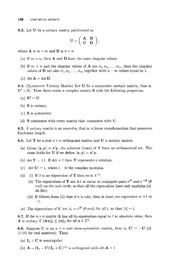
148 SOME SPECIAL MATRICES
8.3. Let U be a unitary matrix partitioned as
where A is m x m and D is n x n.
(a) If m = n, then A and D have the same singular values.
(b) If m < n and the singular values of A are u1, u2,. . . ,urn, then the singular values of D are also u1,u2,. . . ,urn together with n - m values equal to 1.
(c) det A = det D.
8.4. (Symmetric Unitary Matrix) Let U be a symmetric unitary matrix, that is, U' = U. Then there exists a complex matrix S with the following properties.
(a) S2 = U.
(b) S is unitary.
(c) S is symmetric.
(d) S commutes with every matrix that commutes with U
8.5. A unitary matrix is an isometry, that is, a linear transformation that preserves Euclidean length.
8.6. Let T be a real n x n orthogonal matrix and U a unitary matrix.
(a) Given (x,y) = x'y, the columns (rows) of T form an orthonormal set. The same holds for U if we define (x, y) = x*y.
(b) det T = fl. If det = 1 then T represents a rotation
(c) I det UJ = 1, where I . I is the complex modulus.
(d) (i) If X is an eigenvalue of T then so is X-'.
(ii) The eigenvalues of T are fl or occur in conjugate pairs eie and e-Ze (0 real) on the unit circle, so that all the eigenvalues have unit modulus (cf. 16.46b).
(iii) It follows from (ii) that if n is odd, then at least one eigenvalue is +1 or -1.
(e) The eigenvalues of U are X i = eis (0 real) for all i, so that 1x1 = 1.
8.7. If the n x n matrix A has all its eigenvalues equal to 1 in absolute value, then A is unitary if ~ ~ A x ~ ~ 2 5 IIx112 for all x E C".
8.8. Suppose C is an n x n real skew-symmetric matrix, that is, C' = -C (cf. (5.19) for real matrices). Then:
(a) I, + C is nonsingular.
(b) A = (I, - C)(I, + C)-' is orthogonal with det A = 1.
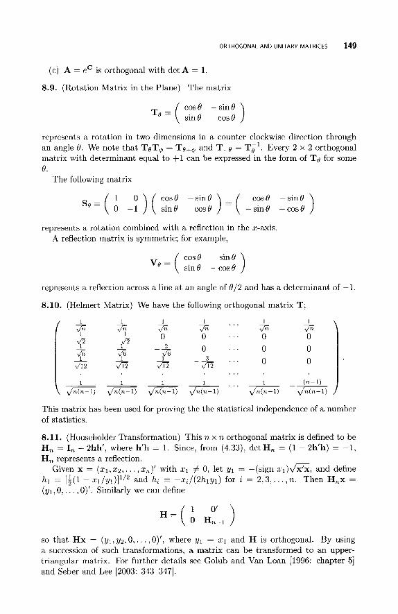
ORTHOGONAL AND UNITARY MATRICES 149
(c) A = ec is orthogonal with det A = 1.
8.9. (Rotation Matrix in the Plane) The matrix
= ( cosO -sin6 sine cos0
represents a rotation in two dimensions in a counter clockwise direction through an angle 0. We note that T Q T ~ = T Q + ~ and T-Q = Tgl. Every 2 x 2 orthogonal matrix with determinant equal to +1 can be expressed in the form of TQ for some e.
The following matrix
-sine ) = ( cos6 -sin0 -sin0 -cosO
represents a rotation combined with a reflection in the x-axis. A reflection matrix is symmetric; for example,
vQ = ( cose sine sin0 -cosO
represents a reflection across a line at an angle of 0/2 and has a determinant of -1.
8.10. (Helmert Matrix) We have the following orthogonal matrix T;
. . 1 1
~ ~ ~ ___ . . . ~ -~
This matrix has been used for proving the the statistical independence of a number of statistics.
8.11. (Householder Transformation) This n x n orthogonal matrix is defined to be H, = I, - 2hh’, where h’h = 1. Since, from (4.33), detH, = (1 - 2h’h) = -1, H, represents a reflection.
Given x = (x1,x2,. . . ,x,)’ with x1 # 0, let y1 = -(sign XI)&&, and define hl = [$(l - ~ l / y 1 ) ] ~ / ~ and hi = -zi/(2hlyl) for i = 2,3 , . . . , 71. Then H,x = (yl, 0 , . . . ,O)’. Similarly we can define
so that H x = (yl , yz, 0 , . . . ,O)’ , where y1 = 2 1 and H is orthogonal. By using a succession of such transformations, a matrix can be transformed to an upper- triangular matrix. For further details see Golub and Van Loan [1996: chapter 51 and Seber and Lee [2003: 343-3471,
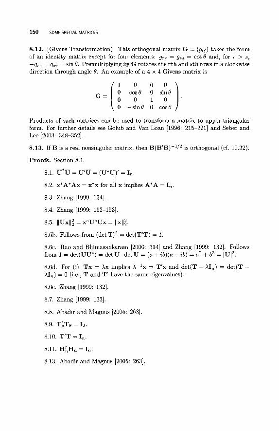
150 SOME SPECIAL MATRICES
8.12. (Givens Transformation) This orthogonal matrix G = ( g i j ) takes the form of an identity matrix except for four elements: grr = gss = cose and, for r > s, -grs = gsr = sin 8. Premultiplying by G rotates the r th and s th rows in a clockwise direction through angle 8. An example of a 4 x 4 Givens matrix is
0 0 0 G = ( co;e ; si;e 1 ,
0 -sine 0 cose
Products of such matrices can be used to transform a matrix to upper-triangular form. For further details see Golub and Van Loan [1996: 215-2211 and Seber and Lee [2003: 348-3521.
8.13. If B is a real nonsingular matrix, then B(B’B)-l12 is orthogonal (cf. 10.32).
Proofs. Section 8.1.
8.1. u*u = U ’ u = (U*U)’ = I,.
8.2. x*A*Ax = x*x for all x implies A*A = I,.
8.3. Zhang [1999: 1341.
8.4. Zhang [1999: 152-1531.
8.5. IlUxll; = x*U*Ux = 11x11;.
8.6b. Follows from (det T ) 2 = det(T’T) = 1
8 . 6 ~ . Rao and Bhimasankaram [2000: 3141 and Zhang [1999: 1321. Follows from 1 = det(UU*) = det U . det u = ( a + ib)(a - ib) = a2 + b2 = IUI2.
8.6d. For (i), Tx = Ax implies X-lx = T’x and det(T - XI,) = det(T - XI,) = 0 (i.e., T and T’ have the same eigenvalues).
8.6e. Zhang [1999: 1321.
8.7. Zhang [1999: 1331.
8.8. Abadir and Magnus [2005: 2631
8.9. TLTo = 1 2 .
8.10. T’T = I,.
8.11. HLH, = I,.
8.13. Abadir and Magnus [2005: 2631.
PERMUTATION MATRICES 151
8.2 PERMUTATION MATRICES
Definition 8.2. Let IIij be the identity matrix I, = (el, ez,, . . e,) with its i th and j t h rows interchanged. Then IIZ = I,, so that IIij is a symmetric and orthogonal matrix. Premultiplying any matrix by IIij will interchange its i th and j t h rows so that IIi, is an (elementary) permutation matrix. Postmultiplying a matrix by an elementary permutation matrix will interchange two columns.
Any reordering of the rows of a matrix can be done using a sequence of elementary permutations 11 = IIiKjK . . . IIi,j,, where
IIn’ = n. . . . . n. . HZlj1 . . . n. . = I,. 2 K 3 K 2131 aK3K
The orthogonal matrix II is called a permutation matrix. The permutation matrix IIo = (en, el, e2,. . . , en-l), which has been called the
forward shaft permutation matrix (and also primary permutation matrix) , is useful in the theory of circulants.
For a helpful discussion of permutations and cyclic permutations see Davis [1979] and Rao and Bhimasankaram [2000: section 6.21.
8.14. IIo has the following properties.
(a) IIoAIIb = (ai+l,j+l) with n + 1 F 1 (i.e., subscripts are taken mod n).
(b) Hg = (e,-i,en,ei,...,en-z)
(c) II; = I,.
(d) II, = F*I’F, where r = diag(l,w,w2,. . . ,wn-’), the wi are the nth roots of
8.15. An n x n permutation matrix II, has exactly one entry in each row and colunmn equal to 1, and zeros elsewhere. For example
1, and F is an n x n Fourier matrix (cf. Section 8.12.2).
0 1 0
0 0 1 n3 = ( 1 0 0 ) (= (eZ,el,e3), say).
Thus 11, consists of I, with its rows resequenced. It is also I, with its columns resequenced, but not necessarily in the same sequence; that is, II, is not neces- sarily symmetric. Left multiplying an rn x n matrix A by 11, produces the same resequences of the rows of A as IIm, while right multiplying by II, does the same for the columns.
8.16. If II, is a permutation matrix, then so is II;, where k is any positive integer.
8.17. If A is n x n, then the diagonal elements of IILAII, are the same elements (rearranged) as the diagonal elements of A.
Definition 8.3. If A is n x n and 11 is a permutation matrix, then the matrix II’AII = II-lAII is said to be permutation similar to A. This concept is linked to irreducibility in (8.101).
Proofs. Section 8.2.
8.14. Davis [1979: 721.
8.16-8.17. Graybill [1983: 2771
152 SOME SPECIAL MATRICES
8.3 CIRCULANT, TOEPLITZ, AND RELATED MATRICES
8.3.1 Regular Circulant
Definition 8.4. An n x n real or complex matrix A is a (regular) circulant if it has the form
a0 a1 a2 ’ . ’ a0 a1 “ ’
a1 a2 a3 . . .
that is, all the elements are equal on the main diagonal and on each of the diagonals parallel to the main diagonal. Note that A is countersymmetric as it symmetric about its main counter (opposite) diagonal. Most authors omit the word “regular” from the definition, but we follow Graybill [1983] and include it so as to be able to distinguish between two types of symmetric circulant below. Thus, if we define ( j - i ) modulo n as
n + j - i , when i > j , when i 5 j , - a ,
then A is a regular circulant if and only if (j-i)ln = (s-r) ln implies that aij = ars. Alternatively, A is a regular circulant if and only if aij = a(j-z) ln . Another way of defining a regular circulant is ai3 = al,, where
m = { j + i - 1 , j y i , n - ( j - i + l ) , j < i .
We can also use the notation A = circ(a0, a l , . . . , ~ ~ - 1 ) . In applications the circu- lants are generally real.
Regular circulants can arise as incident matrices of experimental designs such as the balanced incomplete block design (BIBD) and cyclic designs (e.g., Rao and Rao [1998: 5131). There are other types of circulant such as skew circulants (Davis [1979: 831 and alternating circulants (Tee [2005: 1361).
Definition 8.5. The polynomial p ( z ) = a0 + a l z + . . . + a,-lz”-’ is sometimes called the representer of the circulant and it occurs, for example, in signal process- ing.
8.18. The forward shift permutation matrix IIo of (8.14) can be expressed as r I 0 = circ(0,1,. . . , O ) .
8.19. circ(a0, a l , . . . , an- l ) = p ( I I 0 ) = a0 + alIIo + 8.20. The following conditions are equivalent.
+ . . . + an-1II;-’.
(1) A is an n x n regular circulant.
(2) IIoAIIL = A .
(3) IIbAIIo=A.
8.21. If A is a real regular circulant, then so is the Moore-Penrose inverse A+
CIRCULANT, TOEPLITZ, AND RELATED MATRICES 153
8.22. Let A be a regular circulant. Then:
(a) A* is a regular circulant.
(b) Ak is a regular circulant, where lc is a positive integer.
(c) A-' is also a regular circulant, if A is nonsingular. In this case, to compute A-' we only need to find its first row.
8.23. If A is a regular circulant with first row (ao, a l , a2,. . . , u,-1), and if
z=O:z#q
for some q, then A is nonsingular.
8.24. If A and B are any n x n regular circulants, then AB is a regular circulant and AB = BA.
8.25. If A is a regular circulant, then so is A* (by 8.22a) and A*A (by 8.24), with A*A = AA*. Thus a regular circulant is a normal matrix.
8.26. Let A and C be n x n regular circulants, and suppose there exists a matrix X such that AX = C . Then there exists a regular circulant B such that AB = C.
Definition 8.6. The n x n matrix C h ( h = 1 ,2 , . . . , n - 1) that has ah = 1 and the other a, = 0 is sometimes refered to as a basic circulant matrix. For example, if n = 3,
a0 a1 a2 0 1 0
A = (z; ;; and c1= (; ; ;) Here C1 = circ(0, 1,O). Note that, in general, C1 is the same as IIo of Definition 8.2.
8.27. If CO = I,, then:
n-1
(a) A = CUhch. h=O
(b) C h = C: ( h = 1,2, . . . , n - 1) and C, = I, (by 8.14~).
8.28. (Eigenvalues and Eigenvectors) Referring to (8.14d), we have the following results.
(a) The eigenvectors of C1 are given by
/3 = n-1/2(l1w3,w2J,. . . ,w(n- l ) J ) 1 '
with corresponding eigenvalues XI, = wJ, for j = 0 ,1 , . . . , n - 1, where w = exp(27rz/n) = cos(27r/n) + i s i n ( 2 ~ / n ) and i = G. (Note that the XI, are the n roots of unity.)
(b) Since chx = c:x = X:x, the eigenvectors of c h are still the yJ with eigen- values AhJ = ~3~ ( h , j = 0, I , . . . , n - 1).
154 SOME SPECIAL MATRICES
(c) We now turn our attention to A of (8.27).
(i) A has eigenvectors 7j with (not necessarily distinct) eigenvalues
n- 1 n- 1
x j = C a h w J h = p ( w j ) = C a h w ? , j = 0 , 1 , . . . , n-1 , h=O h=O
where wj = w j , and p ( z ) is given in Definition 8.5 (above 8.18). Note that the -yj are the same for all regular circulants.
(ii) Setting j = 0 in (i), A0 = a0 + a1 + . . . + an-l is always an eigenvalue.
(iii) The eigenvectors are mutually orthogonal, that is, 7;7k = b j k .
(iv) If F is an n x n Fourier matrix (cf. Section 8.12.2), then it is unitary and FAF' = A, that is, AF* = F*A, where A = diag(X1, X2,. . . ,An). Thus the columns of F* are a universal set of right eigenvectors for all regular circulants. Also A = F'AF.
(v) A spectral decomposition of A is given by
n-1
Here 7; is the complex conjugate of 7; obtained by replacing wj in 7j by its complex conjugate
w = exp( -27~2/n) = cos( 27r/n) - i sin( 27rln).
(vi) The matrix -yj$ is a regular circulant that can be written in the form
h=O
(g) The Moore-Penrose inverse of A, which is also a regular circulant, is given by
A' = xAy17j~:, where the summation is over all r nonzero eigenvalues of A, with r = rank A. If r = n then A' = A-' = F*A-'F.
(h) A+ = $ h C h , where +h = cj Xj'W-hj.
8.29. Let A = circ(c1, c2,. . . , cn) be a real n x n regular circulant.
(a) If n is odd and A0 = Ed, ci 2 0 (cf. 8.28f(ii)), then det A 2 0.
(b) If n is even, n = 2r + 2, A0 > 0, and
T + l T+l
1 - 5 - 1 1 2 I C C Z j l ,
j=1 j=1
then det A 2 0.
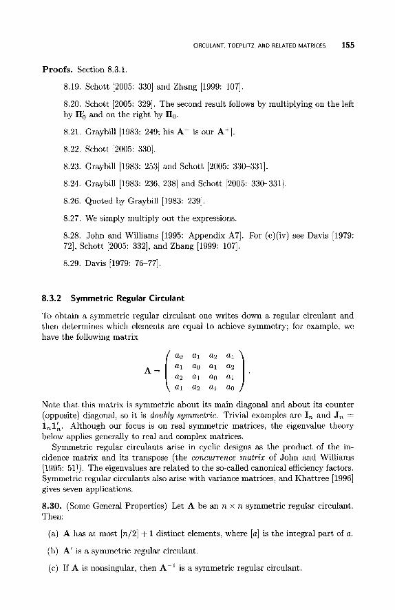
CIRCULANT. TOEPLITZ, AND RELATED MATRICES 155
Proofs. Section 8.3.1.
8.19. Schott [2005: 3301 and Zhang [1999: 1071.
8.20. Schott [2005: 3291. The second result follows by multiplying on the left by IIb and on the right by no. 8.21. Graybill [1983: 249; his A- is our A+].
8.22. Schott [2005: 3301
8.23. Graybill [1983: 2531 and Schott [2005: 330-3311.
8.24. Graybill [1983: 236, 2381 and Schott [2005: 330-3311,
8.26. Quoted by Graybill [1983: 2391.
8.27. We simply multiply out the expressions.
8.28. John and Williams [1995: Appendix A7]. For (c)(iv) see Davis [1979: 721, Schott [2005: 3321, and Zhang [1999: 1071.
8.29. Davis [1979: 76-77].
8.3.2 Symmetric Regular Circulant
To obtain a symmetric regular circulant one writes down a regular circulant and then determines which elements are equal to achieve symmetry; for example, we have the following matrix
a0 a1 a2 a1
A = ( zi z: z:) .
Note that this matrix is symmetric about its main diagonal and about its counter (opposite) diagonal, so it is doubly symmetric. Trivial examples are I, and J, =
1,l;. Although our focus is on real symmetric matrices, the eigenvalue theory below applies generally to real and complex matrices.
Symmetric regular circulants arise in cyclic designs as the product of the in- cidence matrix and its transpose (the concurrence matrix of John and Williams i1995: 511). The eigenvalues are related to the so-called canonical efficiency factors. Symmetric regular circulants also arise with variance matrices, and Khattree [1996] gives seven applications.
8.30. (Some General Properties) Let A be an n x n symmetric regular circulant. Then:
a1 a2 a1 a0
(a) A has at most [n/2] + 1 distinct elements, where [a] is the integral part of a.
(b) A’ is a symmetric regular circulant.
(c) If A is nonsingular, then A-l is a symmetric regular circulant.
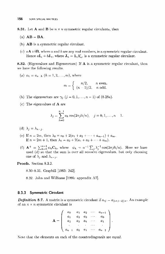
156 SOME SPECIAL MATRICES
8.31. Let A and B be n x n symmetric regular circulants, then
(a) AB = BA.
(b) AB is a symmetric regular circulant.
(c) aA+bB, where a and b are any real numbers, is a symmetric regular circulant. Hence aI, + bJ,, where J , = l n l k , is a symmetric regular circulant.
8.32. (Eigenvalues and Eigenvectors) If A is a symmetric regular circulant, then we have the following results.
(a) ah = an-h ( h = 1 , 2 , . . . ,m) , where
m = { n/2, n even, (n - 1)/2, n odd.
(b) The eigenvectors are ~j ( j = 0,1, . . . , n - 1) of (8.28a).
(c) The eigenvalues of A are
n- 1
~j = C ah cos (2~ jh /n ) , j = 0,1,. . . , n ~ 1. h=O
(d) A, = X n - j .
(e) If n = 2m, then XO = a0 + 2(al + a2 + . . . + u,-I) + a,. If n = 2m + 1, then XO = a0 + 2(al + a2 + . . . + a,).
( f ) A+ = C:I~ $ h C h , where $h = n-1 xj AT' cos(2Tjhln). Here we have used (d) so that the sum is over all nonzero eigenvalues, but only choosing one of X j and An-,.
Proofs. Section 8.3.2.
8.30-8.31. Graybill [1983: 2421.
8.32. John and Williams [1995: appendix A7].
8.3.3 Symmetric Circulant
Definition 8.7. A matrix is a symmetric circulant if az3 = a(,+j-2)ln. An example of an n x n symmetric circulant is
a0 a1 a2 . . . an-1
a2 a3 . . .
. . .
an-l a0 a1 ' . ' an-2
Note that the elements on each of the counterdiagonals are equal.
CIRCULANT, TOEPLITZ, AND RELATED MATRICES 157
8.33. The Moore-Penrose inverse A+ of a symmetric circulant is a symmetric circulant.
8.34. If A is a symmetric circulant and is nonsingular, then Apl is a symmetric circulant .
8.35. Let A be an n x n symmetric circulant with first row elements ao, a l , . . . , anpl and eigenvalues XO, X I , . . . , & - I . If wJ = w, ( j = 0,1, . . . , n - 1; wo = 1) are the n roots of unity, then
j = O j = O j = O
n - 1
+. . . j = O
Also A0 = U, + + . . . + ~ ~ - 1 .
8.36. If A and B are n x n symmetric circulants, then AB is a regular circulant, but, in general, AB # BA.
8.37. If B is a regular circulant and C is a symmetric circulant, then BC and CB are symmetric circulants and, in general, BC # CB.
8.38. Combining the above two results, we have that the product of an even number of symmetric circulants is a regular circulant, and the product of an odd number of symmetric circulants is a symmetric circulant.
8.39. Let A be an n x n regular circulant, C be an n x n symmetric circulant, and suppose there is a solution X to the matrix equation AX = C. Then there exists an n x n symmetric circulant B such that AB = C.
8.40. Let A be a regular circulant, and let B be a symmetric circulant with the same first row uo, a l , . . ., un-l. If the matrices are both n x n, then
det A = (- l)[(n-1)/2] det B,
where [(n - 1)/2] is the integral part of (n - 1)/2.
8.41. Let A be an n x n matrix that is both a symmetric circulant and a symmetric regular circulant. If n is odd, then A takes the form a,, = a for all i , j . If n is even, then A takes the form a,, = a0 if i + j is even and a,j = a1 if i + j is odd.
Proofs. Section 8.3.3.
8.33. Graybill [1983: 249, his A- is our A+].
8.34. Graybill [1983: 2431.
8.35. Graybill [1983: 246-2471
8.36-8.39. Graybill [1983: 244-2451.
8.40-8.41. Graybill [1983: 248-2491,
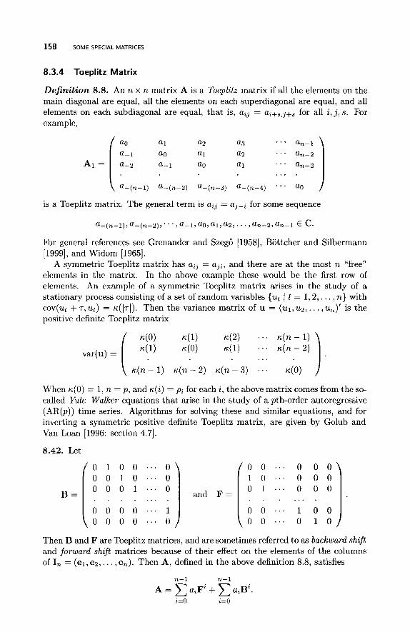
158 SOME SPECIAL MATRICES
8.3.4 Toeplitz Matrix
Definition 8.8. An n x n matrix A is a Toeplztz matrix if all the elements on the main diagonal are equal, all the elements on each superdiagonal are equal, and all elements on each subdiagonal are equal, that is, azJ = az+s,J+s for all i, j , s. For example,
an-1 . . . . . . a-1 . . . a- 1 . . . .
a-(n- l ) a-(n-z) a-(n-3) a-(n-4) ’ ‘ ’
is a Toeplitz matrix. The general term is aa3 = a j p 2 for some sequence
a-(n-l),a-(n-~)r’”,a-lia~,al,a~r.. . ian-2,an-1 E @.
For general references see Grenander and Szego [1958], Bottcher and Silbermann [1999], and Widom [1965].
A symmetric Toeplitz matrix has az j = aJa, and there are at the most n “free” elements in the matrix. In the above example these would be the first row of elements. An example of a symmetric Toeplitz matrix arises in the study of a stationary process consisting of a set of random variables {ut I t = 1,2 , . . . , n} with cov(ut + 7 , u t ) = ~(1.1). Then the variance matrix of u = (u1, u2,. . . ,un)’ is the positive definite Toeplitz matrix
41) K ( 2 ) . . . K ( n - 1) K ( 1 ) . . . K ( n - 2)
. . . var(u) = 4 0 ) ( K:!1) K ( n - 2) K ( n - 3 ) . . . K i o )
When ~ ( 0 ) = 1, n = p , and ~ ( i ) = pz for each 2 , the above matrix comes from the so- called Yule- Walker equations that arise in the study of a pth-order autoregressive (AR(p)) time series. Algorithms for solving these and similar equations, and for inverting a symmetric positive definite Toeplitz matrix, are given by Golub and Van Loan [1996: section 4.71.
8.42. Let
0 0 ” ’ 0 0 0 ( 1 0 . . . 0 0 0 )
- - - ~ ~ 0 1 ‘ . ‘ 0 0 0 \ I 0 0 1 0 ‘ . ’ 0
0 1 0 0 ’ . . 0
Then B and F are Toeplitz matrices, and are sometimes referred to as backward shaft and forward shift matrices because of their effect on the elements of the columns of I n = (el, e2,. . . , en) . Then A, defined in the above definition 8.8, satisfies
n-1 n-1
A = aiFi + aiBa.
i=O i=O
CIRCULANT, TOEPLITZ. AND RELATED MATRICES 159
8.43. A regular circulant is a Toeplitz matrix, but a Toeplitz matrix is not nec- cessarily a regular circulant, though it is sometimes approximated by a regular circulant (cf. Brillinger [1975: 73-74] and the references therein). Any symmetric regular circulant is a symmetric Toeplitz matrix.
8.44. Let A be a Toeplitz matrix.
(a) A’ is also a Toeplitz matrix.
(b) Any symmetric Toeplitz is also doubly symmetric.
(c) If aij is defined by aij = uli-j l , then A is a symmetric Toeplitz matrix.
The case when A is tridiagonal is considered in (8.110).
Proofs. Section 8.3.4.
8.44. Graybill [1983: 284-2871.
8.3.5 Persymmetric Matrix
Definition 8.9. An n x n matrix B = (b i j ) is called persymmetric (countersym- metric) if bij = bn-j+l,n--i+l for all i , j . Such a matrix is symmetric around the counter diagonal. An example is
8.45. Let
0 0 . . . 0 1
- - (0 0 : : : 10) 1 0 . . . 0 0
/ o 0 . . . 0 1 \ 0 0 . ’ . 1 0
1 0 . . . 0 0 = 1 . . . . . . . J >
the so-called exchange permutation matrix. Then, if B is n x n , it is easy to show the following.
(a) If x’ = (xi, 2 2 , . . . , xn) , then (Enx)’ = (zn, xn-lr . . . ,xi).
(b) E,’ =En.
(b) B is persymmetric if and only if B = E,B’En.
(c) If B is persymmetric and nonsingular, then Bpi is persymmetric.
(d) If T is an n x n Toeplitz matrix, then T is persymmetric. The converse is not necessarily true.
160 SOME SPECIAL MATRICES
8.3.6 Cross-Symmetric (Centrosymmetric) Matrix
Definition 8.10. An m x n matrix A = (uzJ) is said to be cross-symmetric (cen- trosymmetric) if atJ = um+l-z,n+l-3 for all i , j and, we call it a C-matrix. For a list of examples of such matrices in statistics and time series see Dagum and Lu- ati [2004]. They also consider a useful transformation and its properties, called a t-transformation, which takes azJ + U ~ + ~ - ~ , ~ + I - ~ .
Note that when m = n:
(1) The elements of the first column read downwards are the same as the ele- ments read upwards in the nth column; the elements in the second column read downwards are the same as the elements read upwards in the (n - 1)th columns; and so forth.
(2) The elements read from left to right in the first row are the same as the elements read from right to to left in the nth row; the elements in the second row read from left to right are the same as the elements read from right to left in the (n - 1)th row; and so forth.
(3) If n is odd, then the middle row (and column) are symmetric about the diagonal element.
An example is ( i ; i ) . 8.3.7 Block Circulant
Definition 8.11. Given an n x n regular circulant matrix with first row elements uo, u2,. . . , un-l, we can construct an n k x nk block circulant matrix A by replacing u j by a k x k matrix Aj ( j = 0,1, . . . , n - 1). Thus
Note that A is not necessarily a regular circulant. Typically each Aj is also a regular circulant or Toeplitz matrix, or it may even be a block circulant with components which are also regular circulants or Toeplitz matrices. For example, in experimental designs we might encounter the symmetric block matrix (n = 2, k = 3)
A =
‘ 4 0 0 I 0 2 2 0 4 0 1 2 0 2 0 0 4 1 2 2 0
0 2 2 1 4 0 0 2 0 2 1 0 4 0
, 2 2 0 1 0 0 4
CIRCULANT. TOEPLITZ. AND RELATED MATRICES 161
Block circulants are used, for example, in n-cyclic designs (cf. John and Williams [1995: 57-58]), while block Toeplitz matrices occur in vector-valued time series.
8.46. A regular circulant of (composite) order n = pq , where p and q are integers, is automatically a block circulant in which each block is Toeplitz. The blocks are of order q, and the arrangement of blocks is p x p (cf. Davis [1979: 70-711). The family of such circulants we denote by B,,q.
8.47. If A E Bp,q, then we have the sum of Kronecker products
A = I, 8 A0 + I I o 8 A1 + IIg @ A2 + . . . + Up-' 0 @ & l >
where I I o is the forward shift permutation matrix of order p (cf. Definition 8.2 in Section 8.2), and the Aj are Toeplitz of order q.
8.48. If A, B E Bp,q and the cri are scalars, then A, A*, crlA + O ~ B , AB, p(A) = C:='=, aiAi, A+ and A-' (if it exists) all belong to Bp,q,. We can use the relationship (8.47) so that AB = BA if AjBk = BkAj for all j , k .
8.49. Let Chk be a basic circulant of order nk (cf. Definition 8.6 below (8.26)), and define the n x n Kronecker product matrix
where n = 121122' . . n,. Then a block circulant matrix A of order n can be defined
nl-1 n z - 1 by
A = C C . .
The eigenvalues and eigenvectors of A Williams [1995: 2321 and Tee [2005]).
Proofs. Section 8.3.7.
h1=0 hz=O
8.47. Davis [1979: 1781.
8.48. Davis [1979: 1811.
n,-1
h,=O
can then be readily found (cf. John and
8.3.8 Hankel Matrix
Definition 8.12. A Hankel matrix A = (a i j ) has the following structure:
aK+1 ,
a0 a1 a2 . ' . a1 a2 a3 . . .
A = [ a2 . a3 . a4 . . . .
a L - 1 a L a L + l . . .
where aij = ai+j-2, so that the elements are equal on each of the counterdiag- onals i + j = const. This matrix arises, for example, from a real time series X = (ao,al , . . . , u N - ~ ) of length N with L the window length (1 < L < N ) and
162 SOME SPECIAL MATRICES
K = N - L + 1; it is called the trajectory matrix of X . If N and L are fixed, then there is a one-to-one relationship between A and X (cf. Golyandina et al. [2001:
If L = K = n, so that A is n x n, then the general term is given by aij = ai+j-2
For further details about Hankel matrices and structured matrices in general see
161).
for some given sequence ao, a l , . . . , azn-3, a2n-2. In this case A is symmetric.
Bini et al. [2001].
8.50. Let II = (en, en-l , . . . ,e l ) be the backward identity permutation matrix. Then:
(a) IIT is a Hankel marix for any Toeplitz matrix T.
(b) IIH is Toeplitz matrix for any square Hankel matrix H.
(c) Since II = II’ = II-’ and square Hankel matrices are symmetric, any Toeplitz matrix is product of two symmetric matrices (II and a Hankel matrix).
Proofs. Section 8.3.8.
8.50. Quoted by Horn and Johnson [1985: 281.
8.4 DIAGONALLY DOMINANT MATRICES
Definition 8.13. Let A = (ai,) be a real or complex n x n matrix (n 2 2), and define
n n
j= 1 : j # p i = l : i # q
to be, respectively, the sum of the absolute values of the off-diagonal elements of the pth row of A, and the sum of the absolute values of the off-diagonal elements of the qth column of A. (In the above, 1x1 denotes the modulus of z if 5 is not real.)
Considering first the rows, if lappl > R,, then the pth row is said to have a strictly dominant diagonal. If lappl 2 R, for p = 1 , 2 , . . . , n, then A is said to be (row) diagonally dominant, while if lapp[ > R, for p = 1,2, . . . , n, then A is said to be strictly (row) diagonally dominant; we denote this by r.d.d. Some authors omit the word “row” and then do not refer to columns. However, there is a corresponding set of definitions for columns. For example, if la,,[ > C,, then the qth column of A is said to have a dominant diagonal, while if la,,[ > C, for q = 1 , 2 , . . . , n, then A is said to be strictly column diagonally dominant and we write c.d.d. If A is either r.r.d. or c.d.d., we say that A is d.d.
8.51. Let A be any n x n matrix (real or complex).
(a) If II is any n x n permutation matrix and A is r.d.d. (respectively c.d.d.), then II’AII is r.d.d. (respectively c.d.d.).
(b) If D is any n x n nonsingular diagonal matrix and A is r.d.d. (respectively c.d.d.), then DA (respectively AD) is r.d.d. (respectively c.d.d.).
(c) If any diagonal element of A is zero, then A is neither r.d.d. nor c.d.d.
DIAGONALLY DOMINANT MATRICES 163
(d) If X is any eigenvalue of A, then A - XI, is neither r.d.d. nor c.d.d
(e) If A is r.d.d. (respectively c.d.d.), then at least one column (respectively row) must have a dominant diagonal.
( f ) If A is a regular circulant with first row elements ao, a l , . . . , a,-l such that
n-1
for some j , then A is nonsingular.
Definition 8.14. Let A a matrix such that
h=l:h#i
Then the j t h column is said to have a dominant element, and it is in the i th row.
8.52. (Conditions for Nonsingularity) Let A be n x n.
(a) (Levy-Desplanques) If A is d.d., then A is nonsingular. Conversely, if A is singular, then A is neither r.d.d. nor c.d.d. This result is linked to (6.29) as 0 cannot then lie in any closed GerSgorin disc, so that 0 is not an eigenvalue.
(b) If R and S are any nonsingular n x n matrices and RAS is a d.d. matrix, then A is nonsingular. Conversely, if A is nonsingular, there exist nonsingular matrices R and S such that RAS is d.d.
(c) Suppose each row, except one (say the kth row), has a strictly dominant diagonal, and suppose the kth row is such that 0 < lakkl = Rk. Then A is nonsingular. A similar theorem exists for columns.
(c) If each column of A has a strictly dominant element, and each row contains one of the dominant elements, then A is nonsingular. This result also holds if each row has a strictly dominant element and these are in distinct columns.
(d) Suppose that for one value of j = 1 , 2 , . . . , n, say j = t , either of the following equations hold, namely
0 < lattl < Rt and laiil. latt[
0 < lattl < Ct and laiil . lattl
> >
RiRt CiCt
for i = 1 , 2 , . . . ,n; i # t for i = 1 , 2 , . . . ,n; i # t ,
then A is nonsingular.
(e) Suppose that all the elements of A are nonzero. If A is diagonally dominant (i.e., not strictly so), and laiil > Ri for at least one value of i = 1,. . . ,n, then A is nonsingular.
8.53. (Positive Determinant) Let A be an n x n real matrix that is d.d. and has positive diagonal elements.
(a) de tA > 0.
164 SOME SPECIAL MATRICES
(b) If A, is any r x r principal submatrix, then det A, > 0.
(c) If the signs of any set of off-diagonal elements are changed, then det A > 0.
(d) The real part of each eigenvalue of A is positive. Thus all real eigenvalues are positive. If, instead, the diagonal elements of A arc all negative, then the real parts of all eigenvalues are negative.
( e ) From (d) it follows that if A is also Hermitian and all its main diagonal elements arc positive, then all the eigenvalues of A are real and positive.
8.54. If A is n x n and T’AT is d.d. with positive diagonal elements, where T is any orthogonal matrix, then det A = det ITI’det A = det(T’AT) > 0 (by 8.6b). Note that T could be a permutation matrix.
8.55. Let A be an n x n matrix that is d.d., and let D be a diagonal matrix with the same diagonal elements as A. Then p(B) < 1, where B = I, - D-lA and p is the spectral radius of B.
8.56. (Linear Equations) Let A be an n x n real matrix with positive diagonal elements and nonpositive off-diagonal elements. For each n x 1 vector b with non- negative elements, there exists a unique vector x with nonnegative elements that is a solution to A x = b if A is d.d.
Proofs. Section 8.4.
8.51. Graybill [1983: section 8.11, here dominant means strictly dominant, and the complex case is mentioned in the note on p. 2611.
8.52. Graybill [1983: 251-256, here dominant means strictly dominant]; also Horn and Johnson [1985: 302 and 355, for (a) and (b) respectively].
8.53. Graybill [1983: 258-261; here dominant means strictly dominant].
8.54. Graybill [1983: 2601.
8.55. Graybill [1983: 2621.
8.56. Graybill [1983: 2651.
8.5 H A D A M A R D MATRICES
Definition 8.15. An n x n Hadamard matrix H is a matrix with elements all f l such that H’H = HH’ = nI,, that is, n-’/2H is orthogonal. If all the elements of the first column arc equal to +1, then H is called a seminormalized Hadamard matrix. If all the elements in the first row and column are equal to +1, then H is said to be normalized. These matrices are closely linked to balanced incomplete block designs, group divisible designs, Youden designs, 2, factorial experiments, optimal weighing designs, and response surface methodology. For further details and applications see Agaian [ 19851.
HADAMARD MATRICES 165
8.57. We have the following properties of an n x n Hadamard matrix H.
(a) H' and nH-' are Hadamard matrices.
(b) If D1 and D2 are diagonal matrices with diagonal elements f l , then DlHD2 is a Hadamard matrix. We can set Di = I, for i = 1 or 2.
(c) n must equal 1 or 2 or be a multiple of 4.
(d) From det(H'H) = nn, det H = fnnI2.
(e) (Hadamard) If A is a real n x n matrix with laijl 5 1, then 1 det A1 5 nnI2. We find that the Hadamard family is the only family of matrices which attains the upper bound.
( f ) If H1 and HZ are n1 x n1 and 722 x 712 Hadamard matrices, respectively, then H1 @ Hz (the Knonecker product) is an n1n2 x n1n2 Hadamard matrix.
(9) Setting n = 2 and applying (f) repeatedly, we see that there is a 2k x 2k Hadamard matrix for every positive integer k .
(h) If an n x n Hadamard matrix exists, then an n x n normalized Hadamard matrix exists.
8.58. In digital signal processing, Hadamard matrices, H, say, are restricted to be of order 2" given by the recursion
H, = H1@Hn-l.
Also Hpn is symmetric so that H& = 2n12,.
8.59. Let H, be defined in (8.58) above, and consider the iteration
Then H, has eigenvalues +2n/2 and -ZnI2, each of multiplicity 2"-', and an eigenvector x, corresponding to the positive eigenvalue 2"12.
8.60. If H is an m x rn Hadamard matrix that contains J, = l n l b , then m 2 n2.
Proofs. Section 8.5.
8.57. Graybill [1983: section 8.14 for (a)-(c)] and Schott [2005: 334-335, for
(C)-(f)l.
8.59-8.60. Zhang [1999: 120-1211.
166 SOME SPECIAL MATRICES
8.6 IDEMPOTENT MATRICES
8.6.1 General Properties
Definition 8.16. An n x n real or complex matrix is said to be idempotent if A2 = A. In Section 2.3 we called such a matrix a projection matrix. If A is also real and symmetric (with (x,y) = x’y), or Hermitian (with (x,y) = y*x), it represents an orthogonal projection matrix. Some other geometrical properties of such matrices are given in Section 2.3. We assume below that A is real, unless otherwise stated, though many of the following results hold for complex matrices.
8.61. The following statements are equivalent.
(1) An n x n matrix P is idempotent.
(2) I, - P is idempotent.
(3) C ( P ) n C(1, - P) = 0.
(4) C ( P ) = N(1, - P).
( 5 ) C(1, - P) = N(P).
8.62. The following statements are equivalent.
(1) A is an n x n idempotent matrix of rank T with Moore-Penrose inverse A+.
(2) There exist orthogonal projection matrices R and S such that A+ = RS.
(3) A + A ’ = A + .
(3) A’A+ = A+.
(4) A = BC’, where C’B = I, with B and C being n x r matrices.
( 5 ) The Jordan canonical form of A (cf. 16.7) can be written as
(6) There exists an orthogonal matrix T such that
where K is T x (n - T ) .
For further results and discussion see Trenkler [1994].
8.63. If A is an n x n idempotent matrix of rank r , then there exist nonsingular R and unitary U such that
R - ~ A R = ( I‘ ) and U * A U = ( ‘a :) for some Q. If A is symmetric, we can replace R by an orthogonal matrix.
IDEMPOTENT MATRICES 167
8.64. An n x n matrix A is idempotent if and only if rankA + rank(1, - A) = n.
8.65. Let A be an n x n idempotent (real or complex) matrix of rank r , then:
(a) A has r eigenvalues equal to 1 and n - T eigenvalues equal to 0. Also, if A is real and symmetric, then it is idempotent if and only if each eigenvalue of A is 1 or 0.
(b) det A’ = det A and det A is 0 or 1. If det A = 1 then, by (a), A = I,.
(c) From (8.63) we have rank A = trace A = r.
(d) I, - A is idempotent and, from (c), rank(1, - A) = n - rankA
(e) A can be expressed in the form A = QR*, where Q and R are n x r and WQ = I,.
( f ) There exists a Hermitian positive definite matrix C such that A = C-lA’C.
8.66. Let A be an n x n matrix with Moore-Penrose inverse A+. Then A is a real symmetic idempotent matrix if and only if one of the following conditions is satisfied.
(1) A’A = A
(2) I - A is symmetric and idempotent.
(3) A is idempotent and AA’ = A’A.
(4) A and A’A are idempotent
(5) AA‘A = A and A is idempotent.
(6) A‘AA’ = A’ and A is idempotent.
(7) A and (A + A’) are idempotent.
(8) AA’ + A‘A = A + A’ and A is idempotent.
(9) I, - 2A is a symmetric, orthogonal matrix.
(10) A’ = A’ and A is tripotent (i.e., A3 = A).
(1 1) AA’ = A’AA’.
(12) A is idempotent and rank(1, - A’A) = n - rank A.
(13) A is idempotent and llAxll2 5 llxllz for all x E R”.
(14) x‘A‘Ax = x’Ax for all x E R”.
(15) A is idempotent and x’Ax 2 0 for all x E R”.
(16) IIy - Ayll’ 5 IIy - xi12 for all y E R” and all x E C(A)
(17) A is idempotent and A = A+.
(18) A is idempotent and AA’ = AA+.
168 SOME SPECIAL MATRICES
(19) A+ = A and A2 = A’.
(20) A and A t are idempotent.
(21) There exists an n x m matrix B such that A = BB+.
(22) A = A A ’
(23) A = B(B’B)-’B for some n x m matrix B of rank m.
See Trenkler [1994] for these and further results of a similar nature. He also gives necessary and sufficient conditions that a symmetric matrix is idempotent.
8.67. (Generalized Inverse and Idempotency) Let A be m x n with Moore-Penrose inverse A+. Then the following conditions are equivalent.
(1) A’A is idempotent (i.e., is an orthogonal projection matrix, because it is symmetric).
(2) AA’ is idempotent.
(3) AA’A = A,that is, A‘ is a weak inverse of A.
(4) A ’ = A + .
8.68. If A is m x n with any weak inverse A-, then N ( A ) = C(I - A-A).
8.69. If (CB)-l exists, then B(CB)-lC is idempotent.
8.70. Let A be an n x n symmetric idempotent matrix, and let B be an n x m matrix of rank m.
(a) If A B = B and rankA = rankB, then A = B(B’B)-lB’.
(b) If A B = 0 and rankA + rankB = n, then A = I, - B(B’B)-lB’
8.71. (Symmetric Matrix) Let A be an
following. n x n symmetric idempotent matrix of rank T , where T < n. Then we have the
(a) 0 5 uz2 5 1 for i = 1 , 2 , . . . ,n.
(b) If ut2 = 0 or uzz = 1, then urg = 0 for all j , j # i.
(c) A is non-negative definite.
(d) If T is orthogonal, then P = T’AT is a symmetric idempotent matrix.
(e) If R is nonsingular, then P = R - l A R is idempotent.
( f ) Q = I, - 2A is a symmetric orthogonal matrix.
(g) We can write A = T,TL, where TLT, = I,, and the columns of T, form an orthonormal basis for C(A). This result holds if A is Hermitian and we replace T’ by T*.
(h) If V is positive definite, then
rank(AVA) = trace(AV)
IDEMPOTENT MATRICES 169
8.72. Let A be a symmetric matrix that satisfies A"' = Ak for some positive integer k . Then A is idempotent.
8.73. Let A1 and A2 be nxn symmetric idempotent matrices, and suppose A1 -A2 is non-negative definite.
(a) AlA2 = A2A1= A2.
(b) A1 - A2 is a symmetric idempotent matrix.
8.74. Suppose A and B are n x n matrices. If AB = A and BA = B, then A and B are both idempotent.
8.75. (Kronecker Products) Let A be mxn and B be m x p real matrices. Let A@B be their Kronecker product, and denote by PA, PB, and P A ~ B the symmetric idempotent matrices that project orthogonally onto C(A), C(B), and C(A @ B). Then:
(a) PABB = PA @ PB.
(b) P A ~ I = PA @ I.
(c) If Q = I - P in each case, then
QABB = QA @ QB + QA @PB +PA @ QB.
8.76. Let A and B be n x n symmetric matrices, with B positive definite. Then AB is idempotent if and only if each eigenvalue of AB is 0 or 1.
Proofs. Section 8.6.1.
8.61(2). Follows directly from (1).
8.61(3). Harville [1997: 384, lemma 17.2.61.
8.61(4). Let P2 = P. If y = Px then (I, - P)y = (I, - P)Px = 0 and y E N(1, - P). Conversely, if (I, - P)y = 0 then y = Py E C(P).
8.61(5). Similar to (4); see Harville [1997: 1461.
8.62. Trenkler [1994]
8.63. Abadir and Magnus [2005: 2341 and Schott [2005: 3961.
8.64. Abadir and Magnus [2005: 2351, Harville [1997: 4351, Rao and Rao [1998: 2531, and Trenkler [1994].
8.65a. Abadir and Magnus (2005: 2331 and Schott [2005: 3971.
8.65e-f. Rao and Rao [1998: 2511.
8.66. Trenkler [1994]
8.67. Trenkler [1994: 2661
8.68. Harville [1997: 1401.
170 SOME SPECIAL MATRICES
8.69. Simply square the matrix.
8.70. Abadir and Magnus [2005: 2361.
8.71a-b. Schott [2005: 3991.
8.71~. Follows from x'Ax = x'A'Ax = y'y
8.71d-e. We have P2 = P.
8.71f. We show that Q'Q = I,.
8.71g. Rao and Rao [1998: 2521 and Seber and Lee [2003: 475, real case]
8.71h. Harville [2001: 82, exercise 101. We have trace(AVA) = trace(AV1/2V1/2A) = trace(V1/2A2V1/2) = trace(V1/2AV1/2) = trace(AV).
8.72. Schott [2005: 3991.
8.73. Seber and Lee [2003: 4651
8.74. Abadir and Magnus [2005: 2361.
8.75. Quoted by Rao and Rao [1998: 2621
8.76. Schott [2005: 3971.
8.6.2
There are many results given for sums of idempotent matrices, and these are of- ten expressed with different conditions. We give several versions of these below, and there is some overlap. For a very general investigation of a linear combination of two projectors see Baksalary and Baksalary [2004a] and the references therein. Questions relating to the nonsingularity of such combinations of idempotent matri- ces, including just sums and differences, are considered by Baksalary and Baksalary [2004b] and Koliha et al. [2004]. We assume below that all matrices are real, unless otherwise stated, though some of the results hold for complex matrices as well.
8.77. If A and B are n x n idempotent matrices, then A + B is idempotent if and only if A B = B A = 0. We generalize this result below.
8.78. (Cochran's Theorem) Suppose A l , A2,. . . , Ak is a sequence of symmetric n x n matrices such that A, = I,. Then the following conditions are equivalent (i.e., each one implies the other two).
Sums of ldempotent Matrices and Extensions
k
(1) A: = Ai for i = 1 , 2 , . . . , k .
(2) A,A, = 0 for all i, j , i # j .
(3) C,"=, rankAi = n.
This can be derived from (8.79) below.
IDEMPOTENT MATRICES 171
8.79. Let A = C,"=, Ai , where each Ai is a symmetric n x n matrix. Any two of the following three conditions implies the third.
(1) A = A'
(2) A: = Ai for i = 1 , 2 , . . . ,n.
(3) AiAj = 0 for all i , j , i # j .
From (8.80) we can include further results involving
k (4) rank A = rank Ail
For example, any two of (l), (2), and (3) implies all four. Furthermore, (1) and (4) imply (2) and (3) (Rao [1973a: 281). We can relate this theorem to the previous one by defining A0 = I, - A so that C,"=oAi = I,. Alternatively, we can set A = I,.
8.80. Let Ai be an n x n matrix (i = 1 , 2 , . . . , k ) , and let A = x:=, Ai
(a) If A2 = A, then the following conditions are equivalent.
(1) AiAj = 0, for all i , j , i # j , and rank A! = rank Ai for i = 1 , 2 , . . . , k .
(2) A: = Ai for i = 1 , 2 , . . . , k .
(3) rankA = Ci=, rankAi. k
If A = I,, then the condition on A is automatically satisfied and rankA = n. Furthermore, if each A, is also symmetric, then A: = AIAi, which implies rank A: = rank Ail and condition (1) reduces to the condition
A,A, = 0 for all i , j , i # j .
(b) If the Ai are all idempotent and AiAj = 0 for all i , j , i # j , then
(i) A' = A.
(ii) rankA = xi=, rankA,. k
(c) Suppose V is an n x n non-negative definite matrix, and let R be any matrix such that V = R'R (cf. 10.10). Then (a) and (b) still hold if we replace each Ai by RAiR' throughout and A by RAR'.
8.81. Let Ai (i = 1 , 2 , . . . , k ) be square (not necessarily symmetric) matrices, and let A = C,"=, A,. Consider the following conditions:
(1) A: = A,, i = 1 , 2 , . . . , k .
(2) AiA, = 0 for all i # j.
(3) A' = A.
(4) xi rank Ai = rank A.
(5) rank(A:) = rank A, , i = 1 , 2 , . . . , k .
172 SOME SPECIAL MATRICES
Then
(2) + (31, (4)i (5)i
(111 (3) + (a), (4)> (51,
(31, (4) + ( I ) , (21, (5).
(2L (3), (5) + ( I ) , (4),
For references to extensions of these results see Tian and Styan [2006]. They also add a new rank subtractivity condition of the form rank(&-A) = n--Cz,l rank A,.
8.82. Let A, ( i = 1 , 2 , . . . , k ) be p x q matrices, and let A = C,=l A,. Consider the following conditions:
k
k
(1) A , A - A , = A 2 , i = 1 , 2 , . . . , k .
(2) A,A-A, = 0 for all i , j , i #
(3) rank(A,A-A,) = rankA,, i = 1,2, . . . , k .
(4) C, rank A, = rank A ,
for some weak inverse A- of A. Then
(1) + (21, (31, (411
(21, (3) -+ (1),(4),
(4) + (1),(2)1(3).
If (1) or if (2) and (3) hold for some weak inverse A- , then (l), (2), and (3) hold for every weak inverse A- .
8.83. Let A; ( i = 1,2, . . . , k ) be an n x n matrix, let A = C,"=, Ai, and let V be a non-negative definite matrix.
(a) If VAVAV = VAV, then each of the following three conditions implies the other two.
(1) VAiVAjV = 0 for all i , j , i # j , and rank(VAiVAiV) = rank(VAiV)
(2) VA,VAiV = VAiV for i = 1,2, . . . , k .
(3) rank(VAV) = x,"=, rank(VAiV).
f o r i = l 1 2 , . . . , k .
When the Ai are symmetric, condition (I) reduces to VAiVAjV = 0 for all i , j , i # j .
(b) If VAiVAiV = VAiV for all i and VAiVAjV = 0 for all i , j , i # j , then:
(i) VAVAV = VAV.
(ii) rank(VAV) = C,"=, rank(VAiV).
A generalization of the above results involving rectangular matrices and an arbitrary rectangular V is given by Tian and Styan [2006]. For related results see Tian and Styan [2005].
IDEMPOTENT MATRICES 173
8.84. Let A be an n x n symmetric idempotent matrix, and let B be a non-negative definite n x n matrix. If I, - A - B is non-negative definite, then AB = BA = 0.
8.85. Let A, be a symmetric idempotent n x n matrix of rank T, ( i = 1,2 , . . . , k ) , and let Ak+l be an n x n non-negative definite matrix such that I, = C,"=': A, =
A + & + I , say. Then:
(a) A,A, = 0 for all i , j = 1,2 , . . . , k + 1, i # j .
(b) k is symmetric and idempotent of rank n - cz=l T,.
8.86. Let A = C,"=, A,, where each A, is an n x n non-negative definite matrix (i = 1 , 2 , . . . , k ) , and let A' = A. If
k
trace A I t r a c e ( x A;), 2=1
then:
(a) Af = Ai for i = 1 '2 , . . . , k .
(b) A,A, = 0 for all i , j , i # j
8.87. Let Ai ( i = 1 , 2 , . . . , k ) be symmetric idempotent matrices such that
k
AiAj = 0, all i , j , ( i # j ) , and x Ai = I,. i= 1
k Then, for positive ai ( i = 1 , 2 , . . . , k ) ,
8.88. Let Ai ( i = 1 , 2 , . . . , k ) be symmetric idempotent matrices such that AiAj = 0 for all i , j , i # j , and let ai, i = 0,1, . . . , k , be positive scalars. Then:
aiAi is positive definite.
aiAi is positive definite.
k (a) V = Q O I , + (b) V-' = POI, + C,"=, BiAi, where
-a( p 0 -ao - -1 and pi = i = 1 , 2 ) . . . , k . Q o ( a 0 + ail '
8.89. Let A be any n x n symmetric matrix of rank T with nonzero eigenvalues Xi
(i = 1,2, . . . , T ) . Then, since A is diagonalizable, A can be expressed in the form (cf. 16.17)
T
i=l
where, for each i = 1 , 2 , . . . , T , Ei is symmetric and idempotent and EiEj = 0 for all i , j , i # j . If A is also idempotent, then
A = EE~. i=l
174 SOME SPECIAL MATRICES
8.90. Let Ai be an n x n symmetric idempotent matrix of rank ri (i = 1 ,2 , . . . , k ) such that CiXl Ai = I,, and let Ci (i = 1 ,2 , . . . , k ) be a p x p square matrix (possibly complex). If
k
k k
are n p x n p , then:
(a) From (8.78) we have AiA, = 0 for all i # j , and C,"=, ri = n.
(b) The eigenvalues of 0 1 and 0 2 are the eigenvalues of C1,. . . , ck with respective
(c) det 0 1 = det 0 2 = n,"=, (det Ci).. .
(d) The matrices 0 1 and 0 2 are nonsingular if and only if all the Ci (i =
algebraic multiplicities T I , . . . , rk.
1 , 2 , . . . , k ) are nonsingular, in which case
k k
This result is used in multivariate error component analysis.
Proofs. Section 8.6.2.
8.77. Harville [1997: 4351 and Schott [2005: 3981.
8.79. Graybill [1983: 4211 and Schott [2005: 4011.
8.80. Harville [1997: 435-4381.
8.81. Anderson and Styan [1982: 31.
8.82. Anderson and Styan [1982: 41.
8.83. Harville [ 1997: 4391.
8.84. C = A(In - A - B)A = -ABA = 0 as C is non-negative definite. Then AB'/2 = 0 and AB = 0.
8.85. Quoted by Graybill [1983: : 4231. For (a) we consider I, - Ai - Aj = (A-Ai-Aj)+Ak, whichisnon-negativedefiniteforall2,j = 1,2, . . . , k + l , (i # j ) , as each Ai is non-negative definite, and then use (8.84). For (b), Ak+l = I, - A, where A is idempotent with rankA = trace A.
8.86-8.88. Graybill [1983: 423, 425-4261.
8.90. Magnus [1982: 242, 2701.
TRIPOTENT MATRICES 175
8.6.3 Products of ldempotent Matrices
8.91. Every singular n x n matrix can be written as the product of idempotent matrices.
8.92. If A and B are n x n idempotent matrices, then AB is idempotent if A B = BA.
Proofs. Section 8.6.3.
8.91. Ballantyne [1978].
8.92. Schott [2005: 3981.
8.7 TRIPOTENT MATRICES
Definition 8.17. An n x n matrix is said to be tripotent if A3 = A. A nonsingular tripotent matrix A is called a involutionary matrix and satisfies A2 = I,. An idempotent matrix is also tripotent.
8.93. (General Properties) Let A be an n x n tripotent matrix.
(a) rankA = trace(A2).
(b) The eigenvalues of A are f l or 0. If n1 are equal to +1, n2 equal to -1 and n3 equal to 0, then:
(i)
(ii) (iii) trace(1, - A2) = 12.3.
(iv) traceA = n1 - 122.
trace(A2 + A) = n1.
trace(A2 - A) = 712.
(c) A is equal to a weak inverse of itself if and only if A is tripotent.
(d) If A is nonsingular, then:
(i) A-' = A .
(ii) A2 = I,.
(iii) ( A + I,)(A - I,) = 0.
(e) If T is orthogonal, then T'AT is tripotent.
( f ) If R is nonsingular, then R-lAR is tripotent.
(g) A2 is idempotent.
(h) -A is tripotent.
8.94. Let A and B be n x n matrices.
(a) If A is symmetric, then A is tripotent if and only if its eigenvalues can only take the values +1, -1, or 0.
176 SOME SPECIAL MATRICES
(b) If A is symmetric, then A is tripotent if and only if there exists two symmetric n x n idempotent matrices C and D such that A = C - D and CD = 0. These two matrices are unique with C = ;(A2 + A) and D = ;(A’ - A). This result has been generalized by Baksalary et al. [2002], and they give conditions for when a linear combination of an idempotent and tripotent matrices is idempotent.
(c) A is tripotent if and only if A’ is idempotent.
(d) If A is symmetric, then A is tripotent if and only if rank A = rank(A+A’) + rank(A - A2).
(e) If A and B are symmetric idempotent matrices and AB = BA, then A - B is a symmetric tripotent matrix.
8.95. Let A, (i = I , 2 , . . . , k ) be square matrices (not necessarily symmetric), and let A = z:=l A,. Consider the following conditions:
( I ) A: = A,, i = 1,2, . . . , k.
(2) A,A, = 0, for all i # j.
(3) A3 = A .
(4) C, rank A, = rank A.
(5) A,A = A:, 2 = I , 2, . . . , k.
(6) APA = A,, i = 1,2 , . . . , k .
(7) A,A = AA,, i = 1 ,2 , . . . , k .
Then (1) and (2) hold if and only if (3), (4), and (5) hold. Condition (5) may be replaced by (6) or (7). Anderson and Styan [1982] prove the above result and a similar result for symmetric matrices. An extension is also given to r-potent matrices, which have the property that A‘ = A, where r is a positive integer.
Proofs. Section 8.7.
8.93. Graybill [1983: section 12.41.
8.94a-b. Graybill [1983: 4321.
8 .94~ . If A3 = A, then = A2. Conversely, if A’ is symmetric and idempotent, its eigenvalues are 0 and there exists orthogonal T such that
and the eigenvalues of A are 0, f l ; then use (a).
8.94d. Anderson and Styan [1982: 131.
8.94e. We multiply out ( A - B)3.
IRREDUCIBLE MATRICES 177
8.8 IRREDUCIBLE MATRICES
Definition 8.18. An n x n matrix A is said to be reducible if and only if, by permuting a set of rows and the corresponding set of columns, A can be transformed
or equivalently of the form
where B11 and B 2 2 are square matrices, i.e., there exists a permutation matrix II such that nAII ' = B. When n = 1 we have A = 0. A matrix that is not reducible is said to be irreducible.
8.96. Given mod(A) = ( la i j l ) , where A is a real n x n matrix (cf. Section 9.1.2), then A is irreducible if and only if (I, + mod(A))n-l > 0 (i.e., every element is positive) or, equivalently, if [I, +Z(A)]"-' > 0, where Z(A) is the indicator matrix of A (each nonzero element is replaced by 1).
8.97. Let A be any n x n real matrix.
(a) If A has no zero elements, then it is irreducible.
(b) If A has zero diagonal elements and nonzero off-diagonal elements, then A is irreducible.
(c) If A is reducible, it must have at least n - 1 elements equal t o zero.
(d) if A has at least one row (column) of zeros, then A is reducible.
8.98. Let A be an n x n irreducible real matrix and let Ri be the sum of the absolute values of the off-diagonal elements of the i th row and Cj the same for the j t h column. Suppose that either laizl >. Ri for i = 1,. . . , n with laii( > Ri for at least one value of i , or lajjl 2 Cj for j = 1, . . . , n with lajjl > Cj for at least one value of j . Then A is nonsingular.
8.99. An n x n (n 2 2) matrix A = ( a i j ) is reducible if aij = 0 for i E S and j @ S for some nonempty proper subset S of { 1 ,2 , . . . , n}.
8.100. The forward shift permutation matrix II, = (en, el , . . . , en-l) is irreducible.
8.101. A permutation matrix is irreducible if and only if it is permutation similar (cf. Definition 8.3 below (8.17)) to a forward shift permutation matrix.
8.102. An n x n permutation matrix is irreducible if and only if its eigenvalues are 1, w, . . . , wn-1 , where w is the nth primitive root of unity.
Proofs. Section 8.8.
8.96. Horn and Johnson [1985: 3611.
8.97-8.98. Graybill [1983: 2641.
8.99. Bapat and Raghavan [1997: 21.
8.100-8.102. Zhang [1999: 124-1251.
178 SOME SPECIAL MATRICES
8.9 TRIANGULAR MATRICES
Definition 8.19. A matrix is lower-triangular if the elements above the main diagonal are all zero. The transpose of this is said to be upper-triangular. A triangular matrix need not be square. A unit triangular matrix is a triangular matrix with unit diagonal elements, and a strictly triangular matrix is a triangular matrix with zero diagonal elements.
8.103. (Basic Properties)
(a) The determinant of a square triangular matrix is the product of the diagonal elements.
(b) The eigenvalues of a square triangular matrix are the diagonal elements.
(c) The inverse of a nonsingular lower (respectively upper) triangular matrix is a lower (respectively upper) triangular matrix.
(d) The product of a finite number of square lower (respectively upper) triangular matrices of the same order is a lower (respectively upper) triangular matrix.
(e) The product of two square unit upper (respectively lower) triangular matrices is unit upper (respectively lower) triangular.
i = 1 , 2 ) . . . ) n.
triangular .
(e) If B is an n x n triangular matrix with inverse C = B-’, then biicii = 1 for
( f ) From (e), the inverse of a nonsingular unit triangular matrix is also unit
8.104. If K is a real lower (upper) triangular matrix and if K’K = KK’, then K is a diagonal matrix.
8.105. (Factorization) Let A be a real square matrix such that every leading prin- cipal minor (excluding A itself) is nonzero.
(a) Then A can be written as the product of a real lower-triangular matrix L and a real upper-triangular matrix U, that is,
A = LU.
Furthermore, if each of the diagonal elements of L (or U) is set equal to unity, then the two triangular matrices are unique. It should be noted that A does not need to be square to have such a factorization, and the reader is referred to Section 16.4 for further details.
(b) If A is also symmetric, then there exists a real upper-triangular matrix U and a diagonal matrix D with diagonal elements equal to fl such that
A = U’DU.
8.106. Every real square matrix A is similar to a triangular matrix (either upper or lower) whose diagonal elements are the eigenvalues of A, that is, there exists a nonsingular matrix R (not necessarily real) such that R-lAR = K, where K is
HESSENBERG MATRICES 179
triangular (and not necessarily real). If the eigenvalues of A are real, then R and K are both real (cf. 16.le).
8.107. If A is a real n x n matrix with real eigenvalues, then there exists an orthogonal matrix T such that T'AT is upper-triangular with diagonal elements the eigenvalues of A (cf. 16.37b).
8.108. (Block Triangular Matrices) An upper block triangular matrix takes the form
where the diagonal blocks are all square matrices of possibly different sizes. We have that
P
det A = n det Aii.
Thus A is nonsingular if and only if all the Aii are nonsingular. In this case A- is also upper block triangular. An algorithm for computing the inverse is given by Harville [1997: 941. Similar results apply for lower block triangular matrices, as the inverse is also lower block triangular.
Proofs. Section 8.9.
i = l
8.103a. Simply expand the determinant by the first row or column depending on whether the matrix is lower- or upper-triangular, respectively.
8.103b. Follows from (a).
8.103~. We use the identity AA-l = I,.
8.103d. Prove for just two matrices first.
8.103e. Use BC = I,.
8.104. Graybill [1983: 2121.
8.105. Graybill [1983: 207, 2101.
8.106. Quoted by Graybill [1983: 211-2121 and proved by Rao and Bhi- masankaram [2000: 288-2891.
8.107. Muirhead [1982: 5871.
8.10 HESSENBERG MATRICES
Definition 8.20. An n x n matrix A is said to be an upper Hessenberg matrix if all its elements below the subdiagonal are zero (i.e., aij = 0 for i > j + 1). Its transpose is called a lower Hessenberg matrix. Upper Hessenberg matrices play an important role in the QR decomposition (Meyer [2000a: 536-5381). Many eigenvalue algorithms reduce their input to a Hessenberg form as a first step, and the latter play a similar role in the Schur decomposition (Golub and Van Loan [1996: section 7.4). Hessenberg matrices appear elsewhere in this book.
180 SOME SPECIAL MATRICES
8.11 TRIDIAGONAL MATRICES
Definition 8.21. An n x n matrix A is tridiagonal if all its elements are zero except those in the middle three diagonals, (i.e., az3 # 0 if Ii - j l 5 1 and uz3 = 0 if Ii - j l > 1). Tridiagonal matrices play a role in matrix decompositions and factorizations-for example, (16.43), (16.45), and (16.46b).
8.109. If A = ( a t j ) is tridiagonal, then expanding cn(A) = det(A1, - A) by the last column we find that
co(X) = 1, cl(A) = (A-al l ) and
.%(A) = (A - azz)cz-l(A) - a ~ , z - ~ a t - ~ , t ~ z - 2 ( A ) r i = 2,3, . . . ,n.
8.110. Suppose that the n x n tridiagonal matrix A is given by
a b 0 . 0 0 0
A =
0 0 0 . c a 0 0 0 ~ 0 c a
where a, b, and c are real or complex. This matrix is both a Toeplitz matrix and a regular circulant .
(a) Then if bc = 0, if u2 = 4bc,
(an+' - p"+')/(a - p) if u2 # 4bc,
a-d- where
2 2 a =
(b) If a is real and bc > 0, the eigenvalues of A are
A, = u + a&cos(jr / (n + I)) , j = 1,2, . . . ,n .
(c) Let b = c so that A is symmetric. Then A is positive definite if and only if the eigenvalues are positive (i.e., a+2bcos(jr/(n+l)) > 0 for j = 1 , 2 , . . . ,T I ) .
A sufficient condition is a > 0 and lb/uI 5 f.
(d) If A is positive definite and b # 0, then B = A-' is given by bi, = bji for i > j and
where y = ( & ) ( d m - 1).
8.111. Given A in (8.110), with a real and bc > 0, then A has real eigenvectors.
TRIDIAGONAL MATRICES 181
8.112. The tridiagonal matrix
. I 1 A = [ . , . . .
0 1 0 . 0 0 0 -cn 0 1 . 0 0 0
0 -cn-l 0 . 0 0 0
0 0 o . - c 3 0 1 0 0 0 . 0 -c2 c1
is called the Schwartz matrix. It often arises in stability analysis. A is positive stable if and only if clcz . . . c, > 0 (cf. Section 8.14.4).
8.113. The inverse of a symmetric n x n matrix B is tridiagonal if and only if for B = 2,3 , . . . , n ,
b,,/bl, = 4 , bl, # 0 for i 5 j 5 n.
This condition means that all the elements on and to the right of the diagonal element in the ith row of B have a constant relation to the corresponding elements of the first row. If B satisfies the above condition, then the inverse B-' = (b',) is given by
b" = -&(b12 - 6'2bll)-l,
br-1,?+1 - @r+ibl,r-l b" = - for T = 2,3,. . . , n - 1,
(br - 1 ,T - or bl ,r - 1 ) (br,,+ 1 - or+ 1 bl ,r ) bnn = - b1,n-l
bl,n(bn-l,n - onb1,n-1)'
br,T-l - - bT-1,r = ( b r - l , r - Orbl,r-l)-l for T = 2,3,. . . , n ,
b'-' = 0 for li - j l > 1.
8.114. (Applications of the Above Result) simply confirm that BB-' = I.
In all of the following cases we can
( 4 If
B =
n n - 1 ' n -2 n - 3 . . . 1 n - 1 2(n-1) 2(n-2) 2(n-3) . . . 2 n - 2 2(n-2) 3(n-2) 3(n-3) . . . 3 n - 3 2(n-3) 3(n-3) 4(n-3) . . . 4
. . . . n . . . 1 2 3 4
,
then B-' is tridiagonal with b'' = 2/(n + 1) for i = 1 , 2 , . . . , n, and b'-l" = b ' ~ ' + ~ = - l / (n+ l ) for i = 2,3,. . . , n- 1. (B is the variance matrix of ordered observations from a random sample of size n from a uniform distribution.)
(b) The autocorrelation matrix of an AR(1) time series is the symmetric Toeplitz matrix a2B, where
1
1 P P2 B = [ p2 p 1 p p2 ' . '
. . . ,,n-l pn-2 ,,n-3 ,,n-4 . . .
182 SOME SPECIAL MATRICES
and IpI < 1, that is, b i j = pli-jl. Then
0 . . . 1 -P - p 1 + p 2 -P . ' .
0 -p 1+p2 . . .
0 0 0 . . . -p 1 . . .
Bpi = (1 - p2)-l
Also B-' = (1 - p2)-'L'L, where
. . . . . . 0 0 . . . -p 1 0 0 0 ." 0 -p 1
JW 0 0 . . . - p 1 0 . . '
L = [ B = u 2 [ 1 1 2 2 3 2 3 2 1 : : " ' 1) 2
0 0
Then det L = Jv and det B = (1 - p2),-l.
( c ) If 1 1 1 1 . ' .
1 2 3 4 ". 4 '
1 2 3 4 . . . n
then
where none of the ai or b j is zero, then
0 0
. . .
. . .
... -
. . .
0
0 0
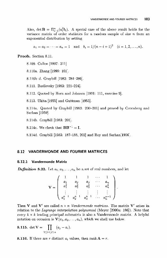
VANDERMONDE AND FOURIER MATRICES 183
Also, de tB = TIr=.=,(a;bi). A special case of the above result holds for the variance matrix of order statistics for a random sample of size n from an exponential distribution by setting
a l = a2 = . . . = a, = 1 and bi = 1/(n - i + 1)2 (i = 1 , 2 , . . . ,n).
Proofs. Section 8.11.
8.109. Cullen [1997: 3111
8.110a. Zhang [1999: 1011.
8.110b-d. Graybill [1983: 284-2861,
8.111. Basilevsky [1983: 221-2241,
8.112. Quoted by Horn and Johnson [1991: 111, exercise 91.
8.113. Ukita [1955] and Guttman [1955].
8.114a. Quoted by Graybill [1983: 200-2011 and proved by Greenberg and Sarhan [ 19591.
8.114b. Graybill [1983: 2011.
8.114~. We check that BB-' = I.
8.114d. Graybill [1983: 187-188, 2021 and Roy and Sarhan[1956].
8.12 VANDERMONDE AND FOURIER MATRICES
8.12.1 Vandermonde Matrix
Definition 8.22. Let al, a2,. . . ,a , be a set of real numbers, and let
1 . . . a2 a3 . . .
1 1
V =
Then V and V' are called n x n Vandermonde matrices. The matrix V' arises in relation to the Lagrange interpolation polynomial (Meyer [2000a: 1861). Note that every k x k leading principal submatrix is also a Vandermonde matrix. A helpful notation on occasion is V(a1, a2, . . . , a,), which we shall use below.
8.115. detV = (a , - a t ) . l<t<jsn
8.116. If there are r distinct a, values, then rankA = r .
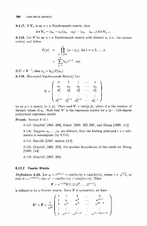
184 SOME SPECIAL MATRICES
8.117. If V, is an n x n Vandermonde matrix, then
det V, = (a, - al)(u, - a2) . . . (a, - a,-1) det V,-1.
8.118. Let V be an n x n Vandermonde matrix with distinct a, (i.e., the inverse exists), and define
n
= n ( x - u j ) , for i = 1 , 2 , . . . , n j = 1 :3#i
n
j = 1
If C = V-l, then cij = bij/Pi(ui).
8.119. (Extended Vandermonde Matrix) Let
1 . . . 1 a2 a3 . . .
be an p x n matrix (n 2 p ) . Then rankV = min(p, d ) , where d is the number of distinct values of ai. Note that V’ is the regression matrix for a ( p - 1)th-degree polynomial regression model.
Proofs. Section 8.12.1.
8.115. Graybill [1983: 2661, Schott [2005: 335-3361, and Zhang [1999: 1111.
8.116. Suppose al, . . . ,a, are distinct, then the leading principal r x r sub- matrix is nonsingular (by 8.115).
8.117. Harville [1997: section 13.61.
8.118. Graybill [1983: 2701. For another formulation of this result see Zhang [1999: 1141.
8.119. Graybill [1983: 2691.
8.12.2 Fourier Matrix
Definition 8.23. Let w = e2Ti/n = cos(27r/n) + isin(27r/n), where i = G, so that W = e-2ai/n; also wr = cos(27rr/n) + i sin(27rrln). Then
F = n-1/2V(1 , i s ,~2 , . . . ,zn-l) is defined to be a Fourier matrix. Since F is symmetric, we have
1 1 1 . . . 1 1 w w2 . . .
. . . 1 Wn-l W2n-2
VANDERMONDE AND FOURIER MATRICES 185
The ( i , j ) t h element is n - ' / ' ~ ( Z - ~ ) ( j - ~ ) . Note that wn = 1, W = w-', w ~ ~ - ~ - -
, w ( , - ' ) ( ~ - ' ) = w, wPi = ~ ~ - 2 , wT = cos(2m/n) + i s i n ( 2 ~ r / n ) , and we have Cj=o waj = 0 if n > 1 and i is an integer such that 0 < i < n (wo = 1). Note that Graybill [1983: 2711 interchanges w and W in his notation so that F looks like F* above, although it is not. Schott [2005: 3311 interchanges F and F*, while Meyer [2000a: 3571 uses 3 = w-' and omits n-1/2 as a multiplier.
8.120. Suppose F is defined above.
(a) F and F* are both symmetric.
(b) F is unitary, i.e., FF* = I,.
(c) F-' =F.
(d) F2 = F*' = II, where 11 is the n x n permutation matrix
W n - 2
n-1
II = (el 1 en, en-1 I . . . , e 2 ) ,
and e, is the i th column of I,.
(e) F4 = F*4 = I,.
( f ) F* can be written as n'/2F* = C +is, where C and S are real matrices with
cij = cos[27r(i - l)(j - l ) /n] and sij = sin[27r(i - l ) ( j - l)/n].
Also CS = SC so that from nFF* we get C2 + S2 = nI,.
(g) The eigenvalues of F are =tl and +i with appropriate algebraic multiplicities.
8.121. Let c,(A) = det(X1, - F*). Then
n = O(mod 4) :
n = l(mod 4) : cn(A) = (A - l)(A4 - l)(1/4)(n-1),
n = 2(mod 4) : c,(A) = (A2 - l)(A4 - 1)('14)+'),
n = 3(mod 4) : &(A) = (A - i ) ( A 2 - 1)(X4 - 1)(1/4)(n-3).
cn(A) = (A - 1)'(A - i ) ( X + l ) ( X 4 - 1)(,14)-',
Definition 8.24. Let y and z be n-dimensional vectors, and let F be an n x n Fourier matrix. Then y = Fz is known as the discrete Fourier transform of the elements of z. Typically, z = ( z (O) , ~ ( l ) , . . . z ( n - l)) ' , a times series sequence, or else z = z(t) (t = 0,1, . . . ,T - l), where z(t) is vector time series. The Fourier transform can be computed using a so-called Fast Fourier Transform Algorithm in which one reduces the calculation of the discrete Fourier transform for a long stretch of data to the calculation of successive transforms of shorter sets of data (cf. Brillinger [1975: section 3.51 and Meyer [2000a: section 5.81). One can also make use of the fact that a Fourier matrix of order 2, can be expressed as Kronecker products (Davis [1979: 36-37]).
Other applications of the transform include the convolution of two time series, computing filtered values from a transfer function, the estimation of the mixing distribution of a compound distribution, and the determination of the cumulative distribution of a random variable from its characteristic function (Brillinger [1975: 67-69]).
186 SOME SPECIAL MATRICES
8.122. If y = Fz then z = F-'y = F*z.
8.123. Let p ( z ) = a, + alz + u2z2 + . . . + an-1zn-' be a polynomial of degree n - 1. It will be determined uniquely by specifying its values p ( z ) at n distinct points z,+ ( k = 1,2, . . . , n) in the complex plane. Suppose we select these points as the n roots of unity, namely, 1, w , w 2 , . . . ,un-l . Then
so that
This gives a relationship between the coefficients of p ( z ) and its values.
Proofs. Section 8.12.2.
8.120. Davis [1979: 31-37] and Graybill [1983: 272-273, with corrections in
MI. 8.121. Carlitz [1959].
8.13 ZERO-ONE (0 , l ) MATRICES
A matrix whose elements are all 0 or 1 is called a (0,l) matrix. I have highlighted this topic as such matrices occur widely throughout statistics. Examples of such matrices are the permutation matrices in this chapter as well as the various vec- permutation and commutation matrices in Chapter 11. There is also the so-called incidence matrix discussed in (8.124) below, and there are Boolean matrices, both of which occur in combinatorial and graph theory. Zero-one matrices play an im- portant role in the solution of equations with large sparse matrices (e.g., Duff et al. [ 19861 ) .
8.124. (Incidence Matrix)
(a) (Experimental Design) The incidence matrix for a block design has a row for each treatment and a column for each block. Thus a 1 for the (i, j ) t h element of the matrix tells us that the ith treatment is applied to the j t h block (cf. John and Williams [1995: chapter 11).
(b) (Non-negative Matrix) As noted by Seneta [1981: 551, many properties of a non-negative matrix A depend only on the positions of the positive and zero elements within the matrix, and not on the actual size of the positive elements. Also, those positions will determine the corresponding positions in all powers Ak, with k a positive integer. This means that in the investigation
SOME MISCELLANEOUS MATRICES AND ARRAYS 187
of the properties of irreducibility and primitivity, the classification of indices into essential and inessential (cf. Section 9.3), and the periodicity of indices that communicate with each other, depend only on the location of the positive elements of A. Therefore given a non-negative matrix A (i.e., all its elements are non-negative), then the matrix obtained by replacing each positive ele- ment by 1 is called the incidence matrix of A. Particular matrices for which incidence matrices have useful applications are stochastic and Leslie matrices. A related (0 , l ) matrix is the indicator matrix, whereby the nonzero elements of any matrix are replaced by 1. For a non-negative matrix, the indicator matrix is the same as the incidence matrix.
8.125. Let A be an n x n (0,l) matrix. If J, = 1,l; and
AA' = ICI, + J,
for some positive integer k , then A is a normal matrix, that is, AA' = A'A.
8.126. If A and B are n x n (0,l) matrices such that AB = J, - I,, then AB = BA.
Definition 8.25. (Boolean Matrix) The binary Boolean algebra B consists of the set (0, l}, together with the usual operations of addition and multiplication (i.e., 1 + O = 1, 0 + 0 = 0, 1 x 0 = 0, 0 x 0 = 0, 1 x 1 = l), except that 1 + 1 = 1. A Boolean matrix is a (0,l) matrix over 8. Boolean matrices have some properties that differ from matrices over R; for example, the row rank need not equal the column rank. Some properties of Boolean matrices and Boolean vector spaces are given by Bapat and Raghavan [1997: section 5.61.
8.127. If T is the incidence matrix of the non-negative matrix A, then Tk is the incidence matrix of A' when T is a Boolean matrix.
Proofs. Section 8.13.
8.125. Zhang [1999: 2511.
8.126. Zhang [1999: 252-2531.
8.127. Seneta [1981: 561.
8.14 SOME MISCELLANEOUS MATRICES A N D ARRAYS
8.14.1 Krylov Matrix
Definition 8.26. If x E R" and A is an n x n matrix, then the matrix
(x, Ax,A2x,. . . , A"-'x)
is called a Krylow matrix. This matrix arises in the so-called Lanczos method of obtaining approximations for some eigenvalues and eigenvectors, especially for large sparse matrices (SlapniEar [2007: chapter 42, 81). The column space of the Krylov matrix is called Krylov subspace, and it is associated with the solution of linear equations (Greenbaum [2007: section 41.11).
188 SOME SPECIAL MATRICES
8.14.2 Nilpotent and Unipotent Matrices
Definition 8.27. An n x n real or complex matrix is nilpotent if A k = 0 for some positive integer k , and is unipotent if A' = I,. For example,
I B A = ( o - I )
is unipotent. For a nilpotent matrix, the smallest k such that Ak = 0 is called the index of nilpotency.
8.128. The eigenvalues of a nilpotent matrix are all zero.
8.129. Let A be a real or complex n x n singular matrix with matrix index k (cf. Section 3.8) such that rank(Ak) = r . Then there exists a nonsingular matrix R such that
R - ~ A R = ( c o ) , where C is a nonsingular r x r matrix and N is nilpotent with k its index of nilpotency.
8.130. If A and B are nilpotent matrices, then so is A + B.
8.131. Any Jordan block J m ( X ) (cf. Definition 16.2) can written as J m ( X ) = XI,+ A,, where A, is nilpotent as (A,), = 0.
More generally, a Jordan matrix can be written as J = D + N, where D is diagonal matrix whose main diagonal is the same as that of J, and N = J - D. Here N is nilpotent as Nk = 0, where k is the order of the largest Jordan block in J.
8.132. Any strictly upper-triangular n x n matrix A is nilpotent with index of nilpotency at most n (as A" = 0). If r j = rank(Aj), then rj+l < rj if rI > 0.
Proofs. Section 8.14.2.
8.128. A x = Ax implies that x # 0 and 0 = A k x = Xkx.
8.129. Meyer [2000a: 3971.
8.130. A' = 0 and B" = 0 for some r and s, which imply ( A + B)T+s = 0.
8.132. Abadir and Magnus [2005: 1831
8.14.3 Payoff Matrix
Definition 8.28. Suppose we have a game consisting of two players I and 11. At each stage of the game, Player I chooses a strategy J with probability yI ( J = 1 , 2 , . . . , n) , where C,"=, yI = 1, and Player I1 independently chooses a strategy z with probability x , ( i = 1 , 2 , . . . ,m) , where CEl z, = 1. Player I1 then pays Player I the amount a z I , or if atI is negative Player I pays Player I1 ( - a z J ) . The m x n matrix A = aZI is called a p a y 0 8 matrzx. (Some authors reverse the roles of the two players so that Player I chooses a strategy i , etc.) The expected zncome to
SOME MISCELLANEOUS MATRICES AND ARRAYS 189
Player I is C,”=, u i j y j , and the game is called a matrix game. Optimal strategies exist for each player, as is proved in (8.133) below.
Let x = ( X I , 5 2 , . . . ,zm)‘ and y = (yl, y z , . . . , yn)’. If x has more than one nonzero element, then the stratgy is called a mixed strategy. If all the elements are positive (i.e., x > 0 ) , the strategy is said to be completely mixed. A matrix game is called a completely mixed game if every optimal strategy x for Player I1 and y for Player I are completely mixed. For further details see Bapat and Raghaven [1997: chapter 11.
8.133. (Minimax Theorem-von Neumann) Let A be an m x n payoff matrix. There exists a unique constant u , called the value of the matrix game A , and mixed strategies x for Player I1 and y for Player I such that
71 n
c a i j y j > u , i = 1 , 2 , . . . , m, and c u i j l c i < u , j = 1 , 2 , . . . , n. j=1 i = l
The strategy x is called an optzmal strategy for Player I1 and y is called an optimal strategy for Player I.
8.134. Let u be the value of a matrix game A , and suppose some optimal strategy of Player I1 is completely mixed. Then, for any optimal strategy y of Player I, A y = v l .
8.135. Let the value of the m x n matrix game A be zero (i.e., u = 0), and suppose that every optimal strategy for Player I1 is completely mixed. Then m - 1 < rankA 5 n - 1. If rankA = m - 1, then the optimal strategy for Player I1 is unique.
8.136. Let A be an n x n matrix with cofactors A,,. If the matrix game A is completely mixed, then C:=l C,”=, A,, is nonzero and the value v of the game is given by
u = det A / ( x A,,) . n n
a = 1 j = 1
Proofs. Section 8.14.3.
8.133. Parthasarathy and Raghaven [1971]
8.134-8.136. Bapat and Raghaven [1997: 10-11, 141.
8.14.4
Definition 8.29. An n x n real or complex matrix A is said to be stable if every eigenvalue of A has a negative real part. The matrix is said to be positive stable if every eigenvalue has a positive real part. These concepts are related to the long- term equilibrium of a dynamical system, and are discussed in detail by Horn and Johnson [1991: chapter 21. For a further discussion see Meyer [2000a: section 7.41.
8.137. exp(At) -+ 0 as t -+ 00 if and only if A is stable (cf. Section 19.6).
Stable and Positive Stable Matrices
190 SOME SPECIAL MATRICES
8.138. If A is an n x n real or complex matrix and
n
se(a i i ) < - C laijl, i = 1,2, . . . ,n; j=l:j#i
where !Re is the real part, then A is stable.
8.139. Suppose A is a positive stable matrix.
(a) A-', A' and A' are all positive stable.
(b) de tA > 0.
(c) Xe(traceA) > 0.
(d) det(Ak) > 0 for any positive integer Ic.
8.140. If A is Hermitian positive definite, then A is positive stable.
8.141. (Lyapunov's Equation) Suppose X, A, and C are all n x n matrices such that X A + A'X = C (see also (13.17~) for further details).
(a) A is positive stable if and only if there exists an Hermitian positive definite solution X such that C is Hermitian positive definite.
(b) Suppose X and C are Hermitian and C is positive definite. Then A is positive stable if and only if X is positive definite.
(c) If A is positive stable, then given C , there is a unique solution X to Lya- punov's equation. If C is Hermitian, then X is Hermitian, while if C is Hermitian positive definite, then X is Hermitian positive definite.
(d) A special case of the above is when C = In, which is Hermitian and positive definite.
Horn and Johnson [1991: 96-98] give a number of generalizations of the above theory.
Proofs. Section 8.14.4.
8.137. Horn and Johnson [1991: 921.
8.138. Marcus and Minc [1964: 1591.
8.139. Horn and Johnson [1991: 931.
8.140. Horn and Johnson [1991: 951.
8.141. Horn and Johnson [1991: 96-98].
SOME MISCELLANEOUS MATRICES AND ARRAYS 191
8.14.5 P-Matrix
Definition 8.30. An n x n real matrix A is called a P-matrix if all its k x k principal minors are positive for k = 1 , 2 , . . . , n.
8.142. Let A be an n x n P-matrix. Then:
(a) A’ is also a P-matrix.
(a) DA and AD are also P-matrices, where D is a diagonal matrix with positive diagonal elements.
(b) Every principal submatrix of A is also a P-matrix.
(c) aii > 0 for i = 1 , 2 , . . . , n .
(d) If II is any n x n permutation matrix, then II’AII is a P-matrix.
(e) A+D is a P-matrix, where D is a diagonal matrix with non-negative diagonal elements.
8.143. Let A be a real n x n matrix. Each of the following conditions is necessary and sufficient for A to be a P-matrix.
(1) For every n x 1 vector x, there is an element in x (say the qth) and the corresponding element in y = Ax such that xqyq > 0.
(2) For every x # 0, there exists a diagonal matrix D, a function of x, with positive diagonal elements such that x’DAx > 0.
(3) For every x # 0, there exists a diagonal matrix D, a function of x, with non-negative diagonal elements such that x’DAx > 0.
(4) Every real eigenvalue of A and of each principal submatrix of A is positive.
Proofs. Section 8.14.5.
8.142. These results quoted by Graybill [1983: 3761 follow directly from the definition.
8.143. Graybill [1983: 3771 and Horn and Johnson [1991: 1201.
8.14.6 Z- and M-Matrices
Definition 8.31. An n x n real matrix A = ( a i j ) for which aij 5 0 for all i , j , i # j is called a 2-matrix. Note that if B is an ML-matrix (cf. Definition 9.11 above (9.43)) then A = -B is a Z-matrix, and vice versa.
A Z-matrix A is called a (nonsingular) M-matrix if it is a nonsingular Z-matrix and A-’ 2 0 (i.e., has non-negative elements). This was the definition introduced by Ostrowski in 1937. An equivalent definition used by Horn and Johnson [1991: 1131 is that A is an M-matrix if it is a Z-matrix and positive stable (cf. Section 8.14.4). I have included the word “nonsingular” to avoid ambiguity as definitions vary in the literature. For example, Bapat and Raghavan [1997: section 1.51 allow an M-matrix to be singular and use a different definition. For general references
192 SOME SPECIAL MATRICES
relating to M-matrices see Varga [1962] and Berman and Plemmons [1994]. Non- singular M-matrices arise in game theory (Bapat and Raghavan [1997: section 1.51).
8.144. A is a Z-matrix if and only if A = sI, - B for some B 2 0 and some real S.
8.145. Let A be an n x n Z-matrix such that A = LU, where L is lower-triangular and U is upper riangular, both with positive diagonal elements. Then:
(a) A has positive leading principal minors including det A itself.
(b) L and U are nonsingular.
(c) The off-diagonal elements of both L and U are nonpositive.
(d) No element of L-' or U-' is negative, and the diagonal elements of L-' and Up' are all positive.
8.146. Let A be an n x n Z-matrix such that each real eigenvalue of A is positive. Let B be a Z-matrix such that A 5 B (i.e., at3 5 b,, for all z , j ) . Then:
(a) A and B are nonsingular.
(b) 0 5 B-' 5 A-' (i.e., A-' - B-' - > 0).
(c) Each real eigenvalue of B is positive.
(d) det B 2 det A > 0.
8.147. (Equivalence of Definitions) Let A be a Z-matrix. Then A is an M-matrix if and only if %(A) > 0 (where ?J2e is the real part) for all eigenvalues A, that is, if and only if A is stable.
8.148. Let A be a Z-matrix. Then each of the following conditions is necessary and sufficient for A to be an M-matrix.
(1) All principal minors of A are positive, including det A; that is, A is a P- matrix.
(2) The leading principal minors of A are all positive, including det A.
(3) Every real eigenvalue of A is positive.
(4) A + tI, is nonsingular for all t 2 0.
(5) A + D is nonsingular for every non-negative diagonal matrix D.
(6) There exists an x > 0 such that Ax > 0.
(7) Ax 2 0 implies x 2 0.
8.149. If A is a Z-matrix, then it is a (nonsingular) M-matrix if and only if it can be expressed in the form A = sI, - B, where B 2 0 and s > p(B), with p(B) being the spectral radius of B.
8.150. If A is an M-matrix, then so is every principal submatrix.
SOME MISCELLANEOUS MATRICES AND ARRAYS 193
8.151. If A is an M-matrix, it is also a P-matrix.
8.152. Let A and B be n x n Z-matrices. If A is an M-matrix and B 2 A (i.e., b,, 2 at3 for all z , j ) , then:
(a) B is an M-matrix.
(b) A-' 2 B-' 2 0.
(c) det B 2 det A > 0.
(d) The matrix A satisfies the Hadamard inequality
de tA 5 al la22. . .a ,,.
(e) A-'B 2 I, and BA-l 2 I,.
( f ) B-'A I I, and AB-l I I,.
(g) AB-' and B-'A are M-matrices
8.153. Let A be an M-matrix. Then there exists a positive eigenvalue of A, XO say, such that the real part of any eigenvalue of A is greater than or equal to Xo.
Proofs. Section 8.14.6.
8.144. Horn and Johnson [1991: 1131. Take cij = max{-ai,,O} and s 2 max,{a,,} so that A = sI, - (C + sI, - diag(al1,. . . ,ann).
8.145. Graybill [1983: 3801.
8.146. Graybill [1983: 380-3811,
8.147. Meyer [2000a: 6261.
8.148. For further equivalent conditions and details see Horn and Johnson [1991: 114-1151. Some proofs are also given by Graybill [1983: section 11.31 and Meyer [2000a: 6261. A game theoretic proof for some of the results like these are given by Bapat and Raghavan [1991: 25-28].
8.149-8.150. Horn and Johnson [1991: 1131 and Meyer [2000a: 6261.
8.152. Graybill [1983: 386, (a)-(g) except (d)] and Horn and Johnson [1991: 117, (a)-(d)I.
8.153. Quoted by Graybill [1983: 3851.
194 SOME SPECIAL MATRICES
8.14.7 Three-Dimensional Arrays
In nonlinear regression models, the expected value of a random response variable yi is usually of the form fi(xi;O), and this leads to looking at afi/aB,i3&, which is a 3-dimensional array. Such arrays have been used for a wide variety of models including nonlinear models (cf. Seber and Wild [1989] and Wei [1997]) and multi- nomial models (e.g., Seber and Nyangoma [2000] and Wei [1997: section 7.21).
Definition 8.32. Consider the n x p x p array W = { (wrS)} made up of a p x p array of n-dimensional vectors w,, (T , s = 1 , 2 , . . . p ) . If wirs is the i th element of w,,, then the matrix of i th elements Wi = (wirs) is called the i th face of W . We now define two types of multiplication. Firstly, if B and C are p x p matrices, then
V = { ( v , ~ ) } = B W C
denotes the array with i th face Vi = BWiC, i.e.,
a 0
Secondly, if D is a q x n matrix, then we define square bracket multiplication by the equation
[Dl [WI = { (DWTs 1 }, where the right-hand side is a q x p x p array.
which is a p 2 x n matrix with i th column vec Wi.
8.154. Using the above notation, we have the following.
We can also define trace W , a vector with i th element traceWi, and vec W ,
( 4 [Inl[Wl = W .
(b) [QB + PCI [WI = +I [WI + PIC1 [WI.
(c) trace[BW] = trace[WB].
(d) BtraceW = trace([B][W]).
(e) vec ([B] [W]) = (vec W)B’.
( f ) [D][BWC] = B[D][W]C.
(g) vec ([BWC]) = (C’ @ B)vec W , where “8” is the Kronecker product.
(h) [DBl[Wl = [Dl[{(Bwrs))l = [Dl“Bl[WlI.
(i) a’Wb = C , C, a,b,w,,,.
(j) [d’][W] is a matrix with (T , s)th element xi diwirs.
Proofs. Section 8.14.7.
8.154. Seber and Wild [1989: 692, (h)-(j)] and Wei [1997: 188-191, (a)-(j)].
CHAPTER 9
NON-NEGATIVE VECTORS AND MATRICES
Any matrix of probabilities has non-negative entries and is therefore a non-negative matrix. Consequently, such matrices play a varied role in probability and statis- tics. For example, they are used in genetic and population growth models, general stochastic processes, and various scaling problems. Such matrices are also encoun- tered in the previous chapter where a number of matrices were mentioned such as permutation matrices, where the elements are zero or one. Non-negative matrices also play an important role in combinatorics (e.g., Sachkov and Tarakonov [2002]). In this chapter we look at a wide range of such matrices. For a concise reference to the subject see Rothblum [2007: chapter 91.
9.1 INTRODUCTION
Definition 9.1. A nonzero matrix A = ( a z J ) is said to be non-negative (positive) if atJ 2 0 (> 0) for all i, j . We write A 2 0 (> 0). Also we say that A 5 0 (< 0) if aZ3 5 0 (< 0). The same definition applies to vectors, namely a 2 0 if a, 2 0 for all i , and a # 0. Finally we say that A 5 B if and only if B - A 2 0.
In most applications, A is square. Unless stated otherwise, we shall assume that A is n x n. Although certain aspects of the general theory of non-negative matrices extend to countably infinite matrices, we shall consider only infinite stochastic matrices (Section 9.6.3).
A M a t n x Handbook for Statastacaans. By George A. F. Seber Copyright @ 2008 John Wiley & Sons, Inc.
195
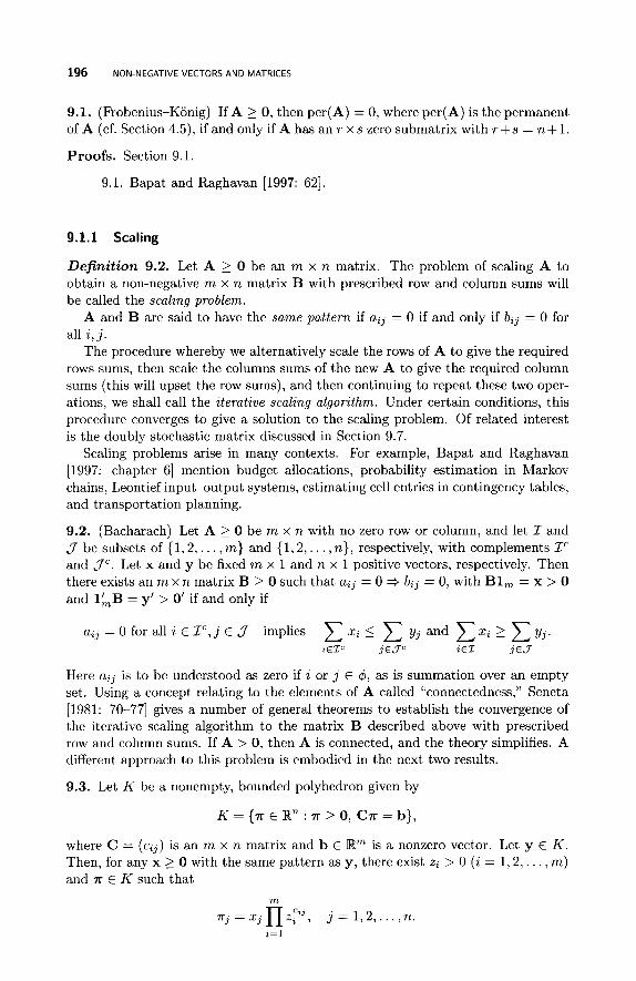
196 NON-NEGATIVE VECTORS AND MATRICES
9.1. (F’robenius-Konig) If A 2 0, then per(A) = 0, where per(A) is the permanent of A (cf. Section 4.5), if and only if A has an r x s zero submatrix with r+s = n + l .
Proofs. Section 9.1.
9.1. Bapat and Raghavan [1997: 621.
9.1.1 Scaling
Definition 9.2. Let A 2 0 be an m x n matrix. The problem of scaling A to obtain a non-negative m x n matrix B with prescribed row and column sums will be called the scaling problem.
A and B are said to have the same pattern if aij = 0 if and only if b,j = 0 for all i , j .
The procedure whereby we alternatively scale the rows of A to give the required rows sums, then scale the columns sums of the new A to give the required column sums (this will upset the row sums), and then continuing to repeat these two oper- ations, we shall call the iterative scaling algorithm. Under certain conditions, this procedure converges to give a solution to the scaling problem. Of related interest is the doubly stochastic matrix discussed in Section 9.7.
Scaling problems arise in many contexts. For example, Bapat and Raghavan [1997: chapter 61 mention budget allocations, probability estimation in Markov chains, Leontief input-output systems, estimating cell entries in contingency tables, and transportation planning.
9.2. (Bacharach) Let A 2 0 be m x n with no zero row or column, and let Z and J be subsets of { 1 ,2 , . . . , m} and { 1 , 2 , . . . , n}, respectively, with complements 2‘ and P. Let x and y be fixed m x 1 and n x 1 positive vectors, respectively. Then there exists an m x n matrix B 2 0 such that aij = 0 + bij = 0, with B1, = x > 0 and 1AB = y‘ > 0’ if and only if
aij = 0 for all i E Z“,j E J implies c xi 5 c yj and cq 2 c IJ~. iEZC j € J c i E l j C 7
Here aij is to be understood as zero if i or j E 4, as is summation over an empty set. Using a concept relating to the elements of A called “connectedness,” Seneta [1981: 70-771 gives a number of general theorems to establish the convergence of the iterative scaling algorithm to the matrix B described above with prescribed row and column sums. If A > 0, then A is connected, and the theory simplifies. A different approach to this problem is embodied in the next two results.
9.3. Let K be a nonempty, bounded polyhedron given by
K = {T E R” : 7r 2 0, C7r = b},
where C = ( c i j ) is an m x n matrix and b E R“ is a nonzero vector. Let y E K . Then, for any x 2 0 with the same pattern as y, there exist zi > 0 (i = 1 , 2 , . . . , m) and 7r E K such that
m
n r - x ’ ~ z , c 2 ’ , 3 - 3 j = l , 2 , . . . ,n. i= 1
SPECTRAL RADIUS 197
Furthermore, any 7r E K of the above type is unique. Bapat and Raghavan [1997: 2471 show how to use this theorem to prove the existence of a solution to the scaling problem.
9.4. Let A and B be any pair of positive m x n matrices. Then there exists a unique matrix C = D1AD2, where D1 and Dz are diagonal matrices with positive diagonal entries, and C and B have the same row and column sums. Also the iterative scaling algorithm applied to A converges to C .
Proofs. Section 9.1.1.
9.2. Bacharach [I9651 and Seneta [1981: 79, exercise 2.341.
9.3. Bapat and Raghavan [1997: 2471.
9.4. Bapat and Raghavan [1997: 251, 2601.
9.1.2 Modulus of a Matrix
Definition 9.3. The modulus of any a real or complex matrix A = (a i j ) is the matrix of absolute values, namely mod(A) = (laijl). Thus mod(A) 2 0. Schott [2005: 3181 uses the term abs(A).
9.5. Clearly A 5 mod(A).
9.6. The following are readily proved using (5.1).
(a) If A and B are any two conformable matrices, then
mod(AB) 5 mod(A)mod(B).
Here B could also be a vector.
(b) If A is square, mod(A'") 5 [mod(A)lk.
(c) If A and B are n x n matrices such that mod(A) 5 mod(B), then
lImod(A)IIF 5 Ilmod(B)IIFj
where 1 1 . [ I F represents the F'robenius norm.
Proofs. Section 9.1.2.
9.6. Quoted by Rao and Rao [1998: 4701.
9.2 SPECTRAL RADIUS
9.2.1 General Properties
We recall that the spectral radius p(A) of a square matrix A is the maximum of the absolute values of the eigenvalues of A. Note that p(A) need not be an eigenvalue of A, though we note below that it can be an eigenvalue in the case of
198 NON-NEGATIVE VECTORS AND MATRICES
non-negative matrices. Although the emphasis is on non-negative matrices in this chapter, further results concerning the spectral radius are given in Section 4.6.2 (e.g., 4.68a) on matrix norms.
9.7. Let A = ( a i j ) be a complex matrix and B = ( b i j ) 2 0 be a real matrix, both n x n, such that mod(A) I B. Then:
(b) (Ky Fan) Every eigenvalue of A lies in the region
9.8. Let A and B be n x n non-negative matrices. If 0 I A I B, then
that is, p(.) is monotonically increasing on the set of all n x n non-negative matrices.
9.9. Let A 2 0 be an n x n matrix.
(a) If C is a principal submatrix of A , then p ( C ) p(A). In particular,
max aii I p(A). l<i<n
(b) Let ri be the row sum of row i and c j be the column sum of column j. Then:
(i) min ri 5 p(A) I max ~ i .
(ii) min cj 5 p(A) 5 l ~ j 2 n c j .
(iii) If ri = a for all i, then p(A) = a. If cj = p for all j , then p(A) = p.
l<i<n l<isn
l<j<n
(c) Let x = (x1,x2,. . . ,xn)' > 0. Then:
(iii) If A has a positive right eigenvector, then
l n l n p ( ~ ) = max min - C aijxj = min max - C aijxj
x > O l<zsn Xi j=l x > O l<z<n Xi j=l
(d) p(In + A ) = 1 + p(A).
9.10. Let A > 0 with maximum and minimum row sums of R and T , respectively, and let m = mini,j aij. Then
T + m(h - 1) 5 p(A) 5 R - m(1 - fl) ,
SPECTRAL RADIUS 199
where
R - 2m + JR2 - 4m(R - r) -r + 2m + Jr2 + 4m(R - r ) , h =
2(r - m) 2m 9 =
There exist matrices for which the bounds are attained.
Proofs. Section 9.2.1.
9.7a. Horn and Johnson [1985: 4911, Meyer [2000a: 6191, and Rao and Rao [1998: 4711.
9.7b. Horn and Johnson [1985: 5011 and Marcus and Minc [1964: 1521.
9.8. Horn and Johnson [1985: 4911.
9.9a. Horn and Johnson [1985: 4911 and Rao and Rao [1998: 4711.
9.9b. Horn and Johnson [1985: 492-4931, Rao and Rao [1998: 4711, and Schott [2005: 318-3191.
9 . 9 ~ . Horn and Johnson [1985: 4931, Rao and Rao [1998: 472, for (i) and (ii)], and Schott [2005: 318-3191.
9.9d. Horn and Johnson (1985: 5071 and Rao and Rao [1998: 4751.
9.10. Marcus and Minc [1964: 1551.
9.2.2 Dominant Eigenvalue
Definition 9.4. If ( A l l > lX2l 2 . . . 2 ( A n [ , then XI is called the dominant eigen- value of A. We note that 1x1 I is also the spectral radius p(A) of A.
9.11. (Perron-Frobenius Theorem for Non-negative Matrices) If A 2 0, then the following hold.
(a) A has a real eigenvalue p 2 0.
(b) With p can be associated non-negative left and right eigenvectors (which need not be unique even when scaled to have unit length).
(c) If A has a positive eigenvector, then the corresponding eigenvalue is p; that is, if Ax = Ax and x > 0, then X = p.
(d) (X I 5 p for any eigenvalue X of A, i.e., p is the spectral radius of A.
(d) If 0 5 B 5 A and f3 is an eigenvalue of B, then If31 5 p.
Seneta [1981: 25-26] gives a helpful history of this and related results. There is a corresponding theorem, originally proved by Perron in 1907 for positive
matrices; for recent proofs see Bapat and Raghavan [1997: 5-61, Rao and Rao [1998: 4731 and Schott [2005: section 8.81. However, when A > 0, A is also irreducible and primitive (see below for definitions), so that a more general theorem is therefore
200 NON-NEGATIVE VECTORS AND MATRICES
given in (9.30). For completeness, we give some related results for A > 0 below in (9.16) from Horn and Johnson [1985] and Schott [2005].
9.12. If A 2 0 and s > p, where p is defined in (9.11) above, then (sI, - A) has an inverse and
(sI, - A)-' 2 0.
9.13. Let A 2 0 with spectral radius p, and let adj(A) denote the adjoint matrix. Then:
(a) B(s) = adj(s1, - A) 2 0 for s > p.
(b) 9 2 0 for s > p.
(c) B(p) 2 0.
(d) $(sI, - A)-'ISEp 2 0.
9.14. Let A 2 0 have spectral radius p.
(a) Suppose x > 0 and a,P 2 0. Then:
(i) If ax 5 Ax 5 px, then a 5 p 5 p. (ii) If ax < Ax, then a < p
(iii) If Ax < px, then p < p.
(b) If x 2 0 (x # 0) and Ax 2 ax for some a, then p 2 a.
9.15. Let A 2 0.
(a) (I, - A)-' exists and is non-negative if and only if there exists x 2 0 such that x > Ax.
(b) If each of the row sums of A is less than 1, then (I, - A)-' exists and is non-negative. The same is true if each of the columns sums is less than 1.
(c) Consider the equation (I,-A)y = b, where b 2 0. If (&-A)-' exists and is non-negative, then there is a unique non-negative solution y = (I, - A)-'b. This result applies, for example, to Leontief's input-output economic model.
An irreducible version of the above theorem is given in (9.36) below.
9.16. (Perron's Theorem for Positive Matrices, with Additions) Suppose A > 0 with spectral radius p = p(A). Then:
(a) p is positive and is an eigenvalue.
(b) There are positive right and left eigenvectors A corresponding to p.
(c) Suppose 1x1 = p, with any corresponding eigenvector x. Then:
(i) Amod(x) = pmod(x), where "mod" is defined in Definition 9.3 above.
(ii) There exists an angle 0 such that e-z'x > 0.
(d) The eigenvalue p has algebraic and geometric mutliplicities both equal to 1.
CANONICAL FORM OF A NON-NEGATIVE MATRIX 201
(e) If X is an eigenvalue of A and X # p, then 1x1 < p.
( f ) Suppose x and y are positive vectors such that Ax = px, y’A = py‘, and x’y = 1. Then:
(i) (A - p ~ y ’ ) ~ = Ak - pkxy‘, for k = 1,2, . . .. (ii) Each nonzero eigenvalue of A - pxy‘ is an eigenvalue of A.
(iii) p is not an eigenvalue of A - pxy‘.
(iv) P(A - PXY? < P. (v) limk,,(p-‘A)k = xy’.
Proofs. Section 9.2.2.
9.11. Debreu and Herstein [1953], Meyer [2000a: 670, (a) and (b)], and quoted by Seneta [1981: 28, exercise 1.121. Horn and Johnson [1985: 4931 prove (c).
9.12. Bapat and Raghavan [1997: 351.
9.13. Bapat and Raghavan [1997: 371.
9.14. Horn and Johnson [1985: 493, 5041
9.15. Rao and Rao [1998: 479-4801.
9.16. Horn and Johnson [1985: 495-5001 and Schott [2005: 319-3231,
9.3 CANONICAL FORM OF A NON-NEGATIVE MATRIX
Definition 9.5. Let A = ( a i j ) 2 0 be n x n, and define A”’ = (ukf”’). If a:;) > 0 for some positive integer m (a function of i and j ) , we say that i leads t o j or i can reach j (or state i can reach state j in the case of a Markov chain and its transition matrix; see Definition 9.16 in Section 9.6), or j is accessible from i, and we write i + j . If i --f j and j + i, we say that the i and j communicate and write i tf j . If i H i, the period of index i is defined to be d ( i ) = gcd{k : ad:) > 0)-that is, the
greatest common divisor of those positive integers k such that aii > 0. If d ( i ) > 1, then i is said to be periodic (cyclic), while if d ( i ) = 1, then i is said to be aperiodic (acyclic). Clearly, if there exists at least one j such that i tf j , we must have i tf i .
The indices can be classified as essential or inessential. If i -+ j , but j f t i for some j , then i is called inessential, and an index which leads to no index at all is also called inessential; otherwise, an index is called essential. Essential indices can be divided into self-communicating classes where all the indices within the class communicate with each other, but do not communicate with any indices outside the class. Similarly, inessential indices (if any) can also be divided into self- communicating classes in which an index in a class can reach another index outside the class, but can’t get back, together with a class of individuals that communicate with no index (Seneta [1981: 121).
9.17. If A 2 0 has at least one positive entry in each row, then it possesses at least one essential class of indices.
( k )
202 NON-NEGATIVE VECTORS AND MATRICES
9.18. If A = (a i j ) 2. 0 and i t i j , then d ( i ) = d ( j ) .
9.19. (Canonical Form) Given A 2 0, there exists a permutation matrix 11 such that
where the Ai (i = 1,2 , . . . . T ) correspond to the T self-communicating classes of essential indices, and Q corresponds to the inessential indices, with R # 0 in general. The matrix B is simply A with the indices reordered, and Q has a structure similar to A, except that there may be nonzero elements to the left of any of its diagonal blocks, that is,
. . .
. . . Q1 0 0 Q2
Q = . . . . . . C
In practice the matrix (R I Q) in B may be missing from B and we could have T = 1. Also
0 . . . 2," . . . x j. . . . . .
s - ( . Ck Q:
Proofs. Section 9.3.
9.17-9.19. Seneta [1981: 14-17].
9.4 IRREDUCIBLE MATRICES
9.4.1 Irreducible Non-negative Matrix
In Section 8.8 we introduced the concept of irreducibiblity for general matrices. In this section we concentrate on non-negative matrices, the major application of irreducibility, and recall the following definition.
Definition 9.6. An n x n non-negative matrix A is said to be reducible if there exist a permutation matrix lI such that
B = IIAII' = ( :tt g2 ) , where BI1 and Bzz are square matrices. A matrix which is not reducible is said to be irreducible. We note that if B has the general canonical form (9.19), then it is
IRREDUCIBLE MATRICES 203
reducible. Some authors use the equivalent definition
An equivalent but more useful definition of irreducibility in the present context is as follows. The n x n matrix A 2 0 is irreducible if and only if every pair of indices in its index set communicate, that is, for every pair i,j there exists a positive integer m (5 n), a function of i and j , such that a!:) > 0. The equivalence of the two definitions is proved by Bapat and Raghavan [1997: 2-41.
An irreducible non-negative matrix is said to be periodic (cyclic) with period d if the period of any one (and so of each one, by (9 .18)) of its indices satisfies d > 1, and it is said to be aperiodic (acyclic) if d = 1.
9.20. An irreducible non-negative matrix cannot have a zero row or column.
9.21. If the matrix A = ( a t j ) 2 0 is reducible, then so is Ak for any positive integer k .
9.22. An n x n non-negative matrix A is irreducible if and only if (I, +A)"-' > 0.
9.23. If A is irreducible, then so is A'.
Definition 9.7. The matrix A 2 0 is said to be primitive if there exists a positive integer p such that AP > 0. (Thus if A is primitive, it is irreducible as a$' > 0 for all i , j . ) Clearly, if A > 0, then A is primitive.
An alternative but equivalent definition is that A 2 0 is primitive if it is ir- reducible and it has only one eigenvalue of maximum modulus. The equivalence follows from (9.26) below.
The smallest positive integer q such that AQ > 0 is called the index ofprimitivity.
9.24. If A 2 0 is primitive, then Ak is non-negative, irreducible, and primitive for all k = 1 , 2 , . . ..
9.25. If A 2 0 is primitive, then Ak > 0 for some integer k 5 (n - l ) n n .
9.26. A non-negative matrix A is primitive if and only if it is irreducible and aperiodic.
9.27. If A 2 0 has att > 0 for all i, then A"-' > 0 and A is primitive.
9.28. (Limit Theorem for Primitive Matrices) Let A be an n x n primitive non- negative matrix with distinct eigenvalues p, X2,. . . , Xt ( t 5 n), where p > 1x21 2 \A3) >_ . . . 2 ] A t ( . In the case lXz l = IX31 (A, # A,) we stipulate that the algebraic multiplicity m2 of A2 is at least as great as that of A3 and of any other eigenvalues having the same modulus as X2. By (9.30) there exist positive vectors x and y such that Ax = px, y'A = py' and x'y = 1. We then have the following:
(a) Suppose A2 # 0.
(i) As k + 03,
Ak = pkxy' + O(k"IX21k)
elementwise, where s = m2 - 1.
204 NON-NEGATIVE VECTORS AND MATRICES
(ii)
Ak lim - = xy'.
k + m pk
(b) Suppose Xz = 0, then for k 2 n - 1,
Ak = pkxy'.
For matrix limits see Section 19.2.
Definition 9.8. An irreducible non-negative matrix that is periodic is said to be imprimitive. Thus irreducible matrices can be subdivided into primitive or imprimitive matrices depending on whether they are aperiodic or periodic.
9.29. The powers of an imprimitive matrix may be studied in terms of powers of primitive matrices.
9.30. (Perron-Fkobenius Theorem for Irreducible Matrices) Let A 2 0 be an irre- ducible matrix. Then we have the following.
(a) A has a real positive eigenvalue p,
(b) With p can be associated strictly positive left and right eigenvalues.
(c) 1x1 5 p for any eigenvalue X of A. Thus p is the spectral radius of A.
(d) p has geometric multiplicity 1, that is, the left and right eigenvectors associ- ated with p are unique to constant multiples.
(e) p has algebraic multiplicity 1, that is, p is a simple root of the characteristic equation.
( f ) If 0 5 B 5 A and /3 is an eigenvalue of B, then 1/31 5 p. Moreover, 1/31 = p implies B = A so that p increases when any element of A increases.
(g) (Primitive matrices) If A is primitive then (a)-(f) still hold except that (c) is replaced by 1x1 < p for any eigenvalue X # p.
Definition 9.9. We call p the Perron-Frobenius eigenvalue of an irreducible non- negative matrix, and its corresponding positive eigenvectors are called the Perron- Frobenius eigenvectors. As noted above, p is the spectral radius.
9.31. Let A 2 0 be an irreducible n x n matrix with Perron-Frobenius eigenvalue p, and let x and y be the right and left Perron-Frobenius eigenvectors of A satisfying x'y = 1. Then:
(a) y'Ax = p 5 x'Ay.
(b) (Limit Theorem) If L = xy', then
k = l
IRREDUCIBLE MATRICES 205
9.32. (Subinvariance Theorem and Variations) Let A 2 0 be an irreducible matrix with Perron-Frobenius eigenvalue p. Let c > 0.
(a) If Ax 5 cx for any nonzero x 2 0, then p 5 c and x > 0. Furthermore, p = c if and only if Ax = cx.
(b) If Ax 2 cx for any nonzero x 2 0, then p 2 c. Also p = c if and only if AX = CX.
(c) If Ax 5 cx (# ex) for some x 2 0, then p < c.
(d) If Ax 2 cx (# cx) for some x 2 0, then p > c.
9.33. (Bounds on p) Let A 2 0 be irreducible with Perron-Frobenius eigenvalue p. Then (9.9b) holds with p(A) = p. In the case of (i) and (ii), equality on one side implies equality on both sides, that is, p can only be equal to a maximal or minimal row (respectively column) sum if all the row (respectively column) sums are equal. The same is true for (c)(i).
9.34. Let P = {x : x > O } . Then:
(4
There also exists an x E P for which both the supremum and the infimum are attained.
(b)
sup { inf *} = p = inf {sup *} . XEP Y E P Y'X X E P YEP Y'X
9.35. Let A 2 0 be irreducible with Perron-Frobenius eigenvalue p, and let E 2 0 (E # 0). If 6 > 0, then B = A + 6E is irreducible with a Perron-Frobenius eigenvalue that, by a suitable choice of 6, may be made equal to any positive number exceeding p.
9.36. Let A 2 0 be irreducible with Perron-Frobenius eigenvalue p.
A necessary and sufficient condition for a solution x (x 2 0 , x # 0) to the equation (sI, - A)x = c to exist for any c 2 0 (c # 0) is that s > p. In this case, there is only one solution x that is strictly positive, and it is given by x = (sI, - A)-'c.
Of those real numbers s for which the inverse exists, (sI - A)-' > 0 if and only if s > p.
If s = 1, then p < 1 if none of the row (or column) sums of A exceed 1, and at least one is less than 1. For applications see Leontief's input-output economic model and an extension described by Bapat and Raghavan [1997: chapter 71, Rao and Rao [1998: 477-4811, and Seneta [1981: chapter 21.
206 NON-NEGATIVE VECTORS AND MATRICES
9.37. Let A 2 0 be irreducible with Perron-Frobenius eigenvalue p = 1. Then the sequence {Ak} converges if and only if A is primitive.
9.38. If A 2 0 is irreducible with Perron-Frobenius eigenvalue p, and Ak = (ulf’), then for each pair ( i , j ) the power series
M
k=O
all have the same radius of convergence R = p- l .
9.39. Suppose A 2 B 2 0 and A # B. If A + B is irreducible, then p(A) > p(B), where p(.) is the dominant eigenvalue of the appropriate matrix.
Proofs. Section 9.4.1.
9.20. Seneta [1981: 181.
9.21. We take powers of B in the definition (e.g., B2 = IIAII’IIAII’ = IIA2II‘).
9.22. Bapat and Raghavan [1997: 31, Rao and Rao [1998: 4691, and Schott [2005: 3241.
9.23. This follows from either definition of irreducibility.
9.24-9.25. Horn and Johnson [1985: 5181.
9.26. Seneta [1981: 211.
9.27. Horn and Johnson [1985: 5171
9.28. Seneta [1981: 91.
9.29. Seneta [1981: 211.
9.30. Bapat and Raghavan [1997: 17, proved the result using the theory of completely mixed matrix games], Horn and Johnson [1985: 508, for (a)-(e)], Schott [2005: 325-326, for (a)-(e)], and Seneta [1981: 22, 3-71,
9.31a. Bapat and Raghavan [1997: 121, with x and y interchanged].
9.31b. Horn and Johnson [1985: 5241.
9.32a. Seneta [1981: 231.
9.32b. Quoted by Seneta [1981: 29, exercise 1.171.
9.32~-d. Debreu and Hurstein [1953].
9.33. Quoted by Seneta [1981: 27, exercise 1.71.
9.34-9.35. Birkhoff and Varga [1958] and quoted by Seneta [1981: 27, exer- cises 1.7 and 1.81.
9.36. Seneta [1981: 30-311.
IRREDUCIBLE MATRICES 207
9.37. Hunter [1983a: 1701.
9.38. Quoted by Seneta [1981: 29, exercise 1.141.
9.39. Quoted by Seneta [1981: 29, exercise 1.161.
9.4.2 Periodicity
Definition 9.10. If A 2 0 is irreducible, then by (9.18) each index a has the same period, d, say, which we call the period of A.
9.40. Let A 2 0 be an irreducible matrix with h eigenvalues whose moduli are equal to the spectral radius p. We know from (9.30~) that h 2 1. Then h = d, the period of A (cf. (9.41b) below).
9.41. Let A 2 0 be an n x n irreducible matrix with period d.
(a) A is primitive if and only if d = 1.
(b) If d > 1, there exist d distinct eigenvalues with (XI = p, where p is the spectral radius. These eigenvalues are pexpi(27rk/d), k = 0,1, . . . , d - 1, the d roots of Xd - pd = 0.
(c) If X # 0 is any eigenvalue of A, then the numbers Xexp[i(27rk/d)], k = 0 ,1 , . . . , d - 1, are also eigenvalues.
(d) The set of n eigenvalues when plotted as points in the complex A-plane is invariant under a rotation of the plane through the angle 27r/d.
(e) Combining (b) and (c),
r
det(X1, - A) = X " ( X d - pd) n(Xd - A t ) , i = l
where IX,I < p for i = 1 , 2 , . . . ,T and m = n - ( T + 1)d.
9.42. Let A 2 0 be irreducible with period d (d > 1).
(a) There exists a permutation matrix 11 such that
0 0 B 2 3 . . . 0 0 Biz 0 . . .
IIAII'= . . . . . 0 0 0 . . . B d - l , d i B d l 0 0 . . .
(= B),
0 0 )
where the zero submatrices on the main diagonal are square. Note that II permutes the rows, while II' permutes the columns in the same order.
(b) Conversely, suppose A 2 0 and there exists a permutation matrix such that IIAII' = B, as defined in (a). If A has no zero rows or columns and B12B23 . . . B d - l , d B d l is irreducible, then A is irreducible.
208 NON-NEGATIVE VECTORS AND MATRICES
Proofs. Section 9.4.2.
9.41a. Seneta [1981: 211.
9.41b. Horn and Johnson [1985: 510, 5121 and Seneta [1981: 231
9 .41~. Seneta [1981: 241.
9.41d. Bapat and Raghavan [1997: 41-42].
9.41e. Bapat and Raghavan [1997: 431.
9.42a. Bapat and Raghavan [1997: 41-42].
9.42b. Seneta [1981: 29, exercise 1.181.
9.4.3
Definition 9.11. An n x n real matrix B = ( b i g ) for which b,j 2 0, for all i , j ( i # j) is called an ML-matrix. This matrix arises in the theory of Markov processes.
9.43. If B is an ML-matrix, there exists a non-negative cy sufficiently large so that
Non-negative and Nonpositive Off-Diagonal Elements
T = &I, + B 2 0.
Definition 9.12. An ML-matrix B is said to be an irreducible ML-matrix if T = cyI, + B 2 0 is irreducible. By taking cy > max, lbzzl, we can make the irreducible T aperiodic and primitive.
9.44. Suppose B is an n x n irreducible ML-matrix. Then there exists an eigenvalue T with the following properties.
(a) T is real.
(b) With T are associated stricly positive left and right eigenvectors, which are unique to constant multiples.
(c) T is greater than the real part of any other eigenvalue X of B, X # T
(d) T is a simple root of the characteristic equation of B.
(e) T 5 0 if and only if there exists y 2 0 (y # 0) such that By 5 0, in which case y > 0; and T < 0 if and only if there is a strict inequality in at least one position in By 5 0.
( f ) T < 0 if and only if A, > 0, i = 1 , 2 , . . . , n, where A, is the principal minor of -B formed from the first i rows and columns of -B.
(g) T < 0 if and only if -B-’ > 0.
9.45. An ML-matrix B is irreducible if and only if eBt > 0 for all t > 0 (see Section 19.6 for matrix exponentials). In this case
eBt = ePtwv’ + O(et l t )
IRREDUCIBLE MATRICES 209
elementwise as t -+ co, where w and v' are the positive right and left eigenvectors of B corresponding to the dominant eigenvalue p of B, normed so that v'w = 1, and having tl < p.
Proofs. Section 9.4.3.
9.43. Choose a = maxi lbii 1 . 9.44-9.45. Seneta [1981: 46-48].
9.4.4 Perron Matrix
Definition 9.13. An n x n matrix A is said to be a Perron matrix (polynomially positive matrix) if f(A) > 0 for some polynomial f with real coefficients. A matrix A is called a power-positave matrzx if Ak > 0 for some positive integer k .
9.46. If A is an irreducible ML-matrix, then it is is a Perron matrix. Also B = -A is a Perron matrix.
9.47. If A 2 0 is irreducible, then f(A) = C,"=, Az > 0 and A is a Perron matrix.
9.48. A power-positive matrix is a Perron matrix. Setting Ic = 1, we see that this includes positive matrices.
9.49. If A is a Perron matrix, then there exists an eigenvalue T such that:
(a) T is real.
(b) With T can be associated strictly positive left and right eigenvectors, which are unique to constant multiples.
(c) T is a simple root of the characteristic equation of A.
9.50. Let A be a Perron matrix with T defined above, and let adj denote an adjoint matrix.
(a) (i) min, C, a,, 5 T 5 max, C, a,,. (ii) min, C, a,, 5 7 5 max, C, a,,.
(b) Either adj(T1, - A) > 0 or -adj(TI, - A) > 0.
(c) If Ax 5 cx for some nonzero x 2 0 and scalar c, then c 2 T ; c = T if and only if Ax = cx.
Proofs. Section 9.4.4.
9.46. From Definition 9.12 we see that A can be written in the form T - aI,, Q > 0, where T is non-negative and primitive, so that for some positive integer k , (A + 9.47. Seneta 11981: 491.
9.48. Set f(x) = x k .
9.49. Bapat and Raghavan 11997: 44, proof using matrix game theory] and Seneta 11981: 491.
9.50. Seneta [1981: 521.
> 0, which is a real polynomial.
210 NON-NEGATIVE VECTORS AND MATRICES
9.4.5 Decomposable Matrix
Definition 9.14. An square matrix A is called partly decomposable if there exist permutation matrices II1 and II2 such that
where B11 and B 2 2 are square matrices. A matrix is said to be ful ly indecompos- able if it is not partly decomposable. Clearly an irreducible matrix is also fully indecomposable, but not necessarily vice versa. A major role of indecomposability is in investigating the combinatorial properties of non-negative matrices.
9.51. If A 2 0 is n x n and fully indecomposable, then A"-' > 0.
9.52. If A and B are non-negative n x n fully indecomposable matrices, then so is A B . (This result is not necessarily true for irreducible matrices.)
Proofs. Section 9.4.5.
9.51. Bapat and Raghavan [1997: 661.
9.52. Bapat and Raghavan [1997: 671.
9.5 LESLIE MATRIX
Definition 9.15. A k x k Leslie matrix for population growth in animal or human populations is a matrix A of the form
f l fz f3 . . ' 6 - 1 fk
A = [ ! ;2 8 1 1 : 8 ! ] , where, for i = 1 , 2 , . . . , k , fi is the average number of daughters born to a single female during the time she is in age class i , and pi is the proportion of females in the ith age class expected to survive and pass into the next age class. (Some authors start the sequences with fo and PO.) These fertility and survival rates are said to be age-specific. Here each fi 2 0 and 0 < p , 5 1, so that A 2 0. In some cases i may refer to a state (stage) rather than age class, and the model is then stage-specific.
The matrix A, and those like it that describe population growth, are sometimes called population projection matrices. Typically, they will contain further non- negative elements such as down the diagonal.
9.53. Let n(t) = (nl(t) ,nz(t) , . . . , n k ( t ) ) ' , where ni(t) is the number of females in the i th age class at time t ( t a positive integer). Then
0 0 0 . . . pk-1
n(t) = An(t - 1) = A t n ( 0 ) ,
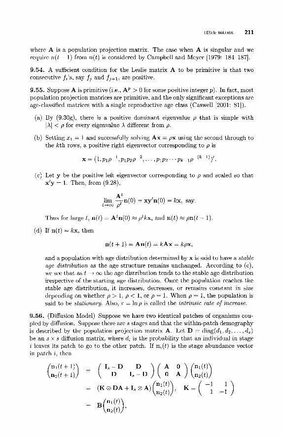
LESLIE MATRIX 211
where A is a population projection matrix. The case when A is singular and we require n(t - 1) from n(t) is considered by Campbell and Meyer [1979: 184-1871,
9.54. A sufficient condition for the Leslie matrix A to be primitive is that two consecutive f i ls , say fj and fj+l, are positive.
9.55. Suppose A is primitive (i.e., A P > 0 for some positive integer p ) . In fact, most population projection matrices are primitive, and the only significant exceptions are age-classified matrices with a single reproductive age class (Caswell [2001: 811).
(a) By (9.30g), there is a positive dominant eigenvalue p that is simple with 1x1 < p for every eigenvalue X different from p.
(b) Setting z1 = 1 and successfully solving Ax = px using the second through to the kth rows, a positive right eigenvector corresponding to p is
(c) Let y be the positive left eigenvector corresponding to p and scaled so that x’y = 1. Then, from (9.28),
At lim -n(O) = x y ’ n ( 0 ) = k x , say.
t-oo pt
Thus for large t , n(t) = A t n ( 0 ) zz p t k x , and n(t) M pn(t - 1).
(d) If n(t) = kx, then
n ( t + 1) = An(t) = k A x = kpx,
and a population with age distribution determined by x is said to have a stable age distribution as the age structure remains unchanged. According to (c), we see that as t + 03 the age distribution tends to the stable age distribution irespective of the starting age distribution. Once the population reaches the stable age distribution, it increases, decreases, or remains constant in size depending on whether p > 1, p < 1, or p = 1. When p = 1, the population is said to be stationary. Also, r = l np is called the intrinsic rate of increase.
9.56. (Diffusion Model) Suppose we have two identical patches of organisms cou- pled by diffusion. Suppose there are s stages and that the within-patch demography is described by the population projection matrix A. Let D = diag(d1, da, . . . , d,) be an s x s diffusion matrix, where di is the probability that an individual in stage i leaves its patch to go to the other patch. If ni(t) is the stage abundance vector in patch i , then
212 NON-NEGATIVE VECTORS AND MATRICES
where B 2 0 and “@” is the Kronecker product. For a general modeling method for patches and stages, see Hunter and Caswell [2005].
An important application of the above theory is the life cycle graph described, for example, by Caswell [2001: chapter 41, where a matrix like A or B is constructed from the graph. A life cycle can also be described as an absorbing finite-state Markov chain, which involves a transition matrix (described below). Caswell [2006] discussed this demographic role of Markov chains in ecology.
Proofs. Section 9.5.
9.54. Demetrius [1971]
9.55. Caswell [200l: 84, section 4.5.21.
9.56. Caswell [200l: 65-66].
9.6 STOCHASTIC MATRICES
9.6.1 Basic Properties
Definition 9.16. A non-negative matrix with each of its row sums equal to 1 is called a (row) stochastic matrix . A common application is the transition matrix of a finite (discrete time) Markov chain in which the i , j t h element of the matrix is the probability of going from state i to state j . In what follows, P is an n x n stochastic matrix with P1, = 1,. When the Markov chain is homogeneous, we are interested in powers Pk of P. For example, if pi0 is the probability that the Markov chain is initially in state i , then p(0) = (p lo ,p20 , . . . ,p,o)’ is the initial probability distribution; after k transitions, the corresponding probability distribution is p ( k ) ,
where pikl = pio Pk. If, as k + 00, p ( k ) tends to a limit that does not depend on the initial probaiility distribution, we say that the process has the ergodic prop- erty. Ergodicity and the so-called coeficient of ergodicity play an important role in more general processes such as inhomogeneous Markov processes and products of inhomogeneous non-negative matrices (cf. Seneta [1981].) The matrix I - P is called the Markovian kernel of the chain, and it has a useful group inverse as well as the usual weak inverse.
If p(o) is such that p ( k ) = p(o) for all k , we say that p(O) is stationary, and a Markov chain with such an initial distribution is said to be stationary. We shall denote this stationary distribution by T, where (setting k = 1) d P = x’ and X’l , = 1.
9.57. If P = ( p Z J ) is A, of P satisfies IX, -
elements, then all the oval
a stochastic matrix and p = mini(pii), then any eigenvalue - pl 5 1 - p . If pii and p j j are the smallest main diagonal eigenvalues of P lie in the interior or on the boundary of the
12 - P i i l l X - P j j l I (1 - Pii)(l - Pjj).
9.58. A stochastic matrix P is irreducible and aperiodic if and only if Pk > 0 for some positive integer k-that is, if and only if P is primitive.
9.59. If P is a stochastic matrix, then so is Pm for any positive integer m.
STOCHASTIC MATRICES 213
9.60. For any stochastic matrix P,
1 lim -(I, + P + p2 + . . . + pk--l ) = R,
k + m k
where R is stochastic and RP = PR = R = R2.
Proofs. Section 9.6.1.
9.57. Quoted by Marcus and Minc [1964: 1611.
9.58. Bapat and Raghavan [1997: 491.
9.59. P"1, = P"-lln = . ' . = 1 n.
9.60. Bapat and Raghavan [1997: 501.
9.6.2 Finite Homogeneous Markov Chain
There is a substantial literature on Markov chains, for example, Hunter [1983b], and more recently, Ching [2006], Hernandez and Lasserre [2003], and Norris [1997], so that I shall consider just some basic results in this section.
9.61. Suppose P, the n x n transition matrix of a finite Markov chain, is irreducible.
(a) Since P1, = l,, P has an eigenvalue equal to 1. However, since the row sums are all equal, it follows from (9.9b(iii)) that p = 1 with a positive right eigenvector of 1,. If q is a positive left eigenvector (i.e., q'P = q'), we can scale q such that q'l, = 1; thus q represents a probability distribution.
(b) q'pk = q'Pk-1 = . . . - - q'.
(c) The irreducible Markov chain has a unique stationary distribution r, the solution of d P = T' and dl, = 1. We can identify 7r with q of (a).
9.62. Suppose that the n x n transition matrix P is irreducible with stationary distribution 7r. Then:
(a) If t and u are any n x 1 vectors, then (I, - P + tu') is nonsingular if and only if d t # 0 and u'l, # 0. If the latter conditions hold, then (I, - P + tu')-* is a weak inverse of I, - P. Furthermore, any weak inverse can be expressed in the form
(I, - P + tu')-' + 1,f' + gn', where f and g are arbitrary vectors.
In addition to the above weak and Moore-Penrose inverses, Hunter [1988] gives expressions for other types of generalized inverses. For further results see Hunter [1990, 19921.
9.63. Suppose P is a primitive stochastic matrix (i.e., irreducible and aperiodic). Using the above notation, we have the following special case of (9.28).
214 NON-NEGATIVE VECTORS AND MATRICES
(a) lim Pk = 1 , ~ ’ (= Qo, say), where 7r is the unique stationary distribution.
(b) If p is a probability distribution (i.e., p’l, = l ) , then
k + m
lim p’pk = ~ ’ 1 ~ 7 ~ ’ = d. k - c c
(c) QO is idempotent.
(d) PQ;T- = QoPm = QO for all integers m 2. 1.
(e) Qo(P - Qo) = 0.
(f) Every nonzero eigenvalue of P - QO is also an eigenvalue of P .
9.64. Suppose that a general stochastic matrix P is expressed in the canonical form of (9.19), where Q # 0. Here Q refers to the submatrix of P associated with transitions between the inessential states, and P is reducible.
(a) Qk + 0 elementwise and geometrically fast as k -+ co.
(b) (I, - Q)-’ exists. In finite absorbing chains, this matrix is sometimes called the fundamental matrix of absorbing chains.
Definition 9.17. An n x n stochastic matrix P is said to be regular if its essential indices form a single class that is aperiodic. In this case P can be expressed in the canonical form (cf. 9.19)
where P1 is a stochastic irreducible aperiodic (primitive) matrix.
9.65. Suppose P is regular with canonical form described above. Let ql be the unique stationary distribution of PI, and define q’ = (ql, 0’) to be an 1 x n vector. Then, as k --f co,
elementwise, where q‘ is the unique stationary distribution corresponding to the matrix P , the approach to the limit being geometrically fast. Thus the regularity of P is a sufficient condition for ergodicity; it is also a necessary condition.
9.66. If an n-state homogeneous Markov chain contains at least two essential classes, then any weighted linear combination of the stationary distribution vec- tors corresponding to each class, each appropriately augmented by zeros to give an n x 1 vector, is a stationary distribution of the chain.
Proofs. Section 9.6.2.
Pk --f 1,q’
9.61. Seneta [1981: 118-1191.
9.63. Rao and Rao [1998: 483, with Q instead of Qo].
9.64. Seneta [1981: 120-1231.
9.65. Seneta [1981: 127; 134, exercise 4.91.
9.66. Quoted by Seneta [1981: 134, exercise 4.121.
STOCHASTIC MATRICES 215
9.6.3 Countably Infinite Stochastic Matrix
In this section we consider a stochastic matrix with a countable (i.e., finite or denumerably infinite) index set { 1 ,2 , . . .}, with our focus on the infinite case. The matrix P = ( p i j ) will still represent a stochastic matrix, but with infinite row sums adding to unity. As matrix multiplication readily extends to infinite matrices, Pk = (pi;)) is well-defined for k = 1 , 2 , . . ., and it is also stochastic (Seneta [1981: chapter 51). However, a more sensitive classification of indices is now required.
Definition 9.18. Let
and k = 1,2, . . . , r:r#i
with 1:;) = 0, by definition, for all i, j E { 1,2, . . .}. Define, for each i and j,
M M
k=O k = l
An index i (or state i) is said to be recurrent if Lii = 1 and transient if Lii < 1. A recurrent index i is said to be positive- or null-recurrent depending on whether pi < 00 or pi = 00, respectively. Here pi is called the mean recurrence measure of i . Note that in the Markov chain context, 1:;' is the probability of going from state i to state j in k steps (or in time k ) , without revisiting i in the meantime. Thus Lii can bc regarded as the probability of staying in or returning to state i for the first time. Also pi is the mean recurrence time of state i . Thus a state i is recurrent if, starting from state i , we will eventually return to state i with certainty. If state i is transient, then there is a positive probability that the system will never return to state i.
9.67. An inessential index is transient and a recurrent index is essential.
9.68. If i is a recurrent aperiodic index and j is any index such that j -+ i (cf. second part of Definition 9.5 in Section 9.4.1), then
In Darticular
Proofs. Section 9.6.3.
9.67. Seneta [1981: 165-1661.
9.68. Seneta [1981: 1711
9.6.4 Infinite Irreducible Stochastic Matrix
The definition of irreducibility given by Definition 9.6 (second definition) applies to infinite matrices; that is, A 2 0 is irreducible if and only if every pair of indices i and j communicate.
216 NON-NEGATIVE VECTORS AND MATRICES
9.69. The following hold for an infinite irreducible stochastic matrix.
(a) Every index has the same period.
(b) The indices are all transient, or all null-recurent, or all positive-recurrent.
Definition 9.19. In the light of (9.6913) we say that an irreducible P is a transient, or null-recurrent, o r positiue-recurrent matrix depending on whether any one of its indices is transient, or null-recurrent , or positive-recurrent .
If v’P = v’ and v is a nonzero non-negative (countably infinite) vector, we call v an invariant measure. Note that a multiple of such a measure is still a measure.
9.70. (General Ergodic Theorem) We have the following series of limits.
(a) Let P be a primitive (i.e., irreducible and aperiodic) stochastic matrix. If P is transient or null-recurrent, then for any pair of indices i , j , we have pi:) + 0 as k --t 00. If P is positive-recurrent,
and the vector x = (p; ’ ) is the unique stationary distribution (invariant vector) satisfying x’P = x’ and Czl xi = 1. The question of computing a finite dimensional approximation for x is discussed by Seneta [1981: section 7.21.
(b) If P is irreducible and periodic with period d, then
9.71. If P is an irreducible transient or null-recurrent matrix, then there exists no invariant measure v’ satisfying v’l < co.
Proofs. Section 9.6.4.
9.69. Seneta [1981: 1721.
9.70. Seneta [1981: 177 for (a); 196, exercise 5.1, for (b)].
9.71. Seneta [1981: 1781.
9.7 DOUBLY STOCHASTIC MATRICES
Definition 9.20. A square n x n matrix A = ( a z J ) is doubly stochastic if A 2 0 and all its column sums and row sums are 1. Some examples of doubly stochastic matrices are given by Marshall and Olkin [1979: 45-48]. For a reference to doubly stochastic matrices see Bapat and Raghavan [1997: chapter 21.
Definition 9.21. The diagonal of a matrix A associated with the permutation 7-r is the set { a l n ( l ) , a2,+), . . . , a n a ( l ) } , and the corresponding diagonal product is n:=l azn(a). A diagonal is said to be positive if each element aaa(a) in the diagonal is positive.
DOUBLY STOCHASTIC MATRICES 217
Definition 9.22. The matrix A is said to have a doubly stochastic pattern if there exists a doubly stochastic matrix with the same pattern of zeros as A.
9.72. A doubly stochastic matrix has a positive diagonal. An algorithm for finding such a diagonal is also available.
9.73. Let A = (azJ) be an n x n doubly stochastic matrix, and let y1 2 yz 2 . . . 2 yn. Then
k k n c Yz 2 U 2 J Y J , k = 112, . . . , n. 2=1 Z = l J = l
9.74. The product of a finite number of doubly stochastic matrices is doubly stochastic.
9.75. If n x n A is doubly stochastic and nonsingular, then A-' has row and column sums equal to 1, but it need not have non-negative elements.
9.76. If A 2 0 is n x n matrix with row totals and column totals not exceeding unity, then there exists a doubly stochastic n x n matrix B such that B 2 A.
9.77. (Scaling) If A is a non-negative n x n matrix with doubly stochastic pattern, then there exist diagonal matrices D1 and Dz with positive diagonal elements such that C = DlADz is doubly stochastic.
9.78. If A is non-negative definite and doubly stochastic and has azz 5 l / ( n - 1) for each i , then the non-negative definite square root A'/' (cf. 10.8) is doubly stochastic.
9.79. Every permutation matrix is a doubly stochastic matrix, because there is a single 1 in every row and column and the remaining elements are zero.
9.80. (Birkhoff-von Neumann) A matrix is doubly stochastic if and only if it is a convex combination of the permutation matrices.
9.81. The set of doubly stochastic matrices is the convex hull of all n x n permu- tation matrices (of which there are n), and the latter constitute the extreme points of this set.
9.82. Let A = (uzJ) be a doubly stochastic n x n matrix.
(a) The permanent (cf. Section 4.5) of A is positive.
with equality if and only if azJ = n-l for all i , j .
9.83. The matrix (azJ) = (n-') is the unique irreducible idempotent n x n doubly stochastic matrix.
9.84. If T = ( t t J ) is a real orthogonal matrix, then A = (t,2,) is doubly stochastic.
9.85. If A 2 0 is n x n (A # 0 ) , then A has a doubly stochastic pattern if and only if every positive entry of A is contained in a positive diagonal.
218 NON-NEGATIVE VECTORS AND MATRICES
Definition 9.23. A matrix A = (az,) is said to be orthostochastzc if there exists an orthogonal matrix T such that a,, = t:,. If there exists a unitary matrix U = (u,,) such that a,, = Iuy 1 2 , then A is said to be unztary-stochastzc (Marshall and Olkin [1979: 231).
Definition 9.24. A square matrix A is said to be doubly substochastzc if A 2 0 and all row and column sums are at most 1.
9.86. The set of all n x n doubly substochastic matrices is a convex set.
9.87. From the definition we have that any square submatrix of a doubly sub- stochastic matrix is doubly substochastic.
9.88. If A = (az,) is doubly substochastic, then there exists a doubly stochastic matrix B = (bz3) such that a,, 5 b,, for all z , ~ .
9.89. If A = (a,,) and B = (b2,) are doubly substochastic, then their Hadamard (Schur) product A o B = (u2,b2,) is doubly substochastic.
Proofs. Section 9.7.
9.72. Bapat and Raghavan [1998: 63-66].
9.73. Anderson [2003: 6461.
9.74. Marshall and Olkin [1979: 201.
9.75. Al, = 1, implies 1, = A-ll,, and A’l, = 1, implies 1, = A-l’l,.
9.76. Bapat and Raghavan [1997: 751.
9.77. Bapat and Raghavan [1997: 871.
9.78. Marshall and Olkin [1979: 511.
9.80. Bapat and Raghavan (1997: 631, Rao and Rao [1998: 314-3151, and Zhang [1999: 1271.
9.81. Marshall and Olkin [1979: 191 and Rao and Rao [1998: 308-3091.
9.82. Bapat and Raghavan [1997: 931 and Rao and Rao [1998: 3141.
9.83. Marshall and Olkin [1979: 191.
9.84. Follows from the fact that the rows and columns of an orthogonal matrix each have unit length.
9.85. Bapat and Raghavan [1997: 681.
9.86. Follows immeditately from the idea of a convex combination.
9.88. Horn and Johnson [1991: 1651 and Marshall and Olkin [1979: 251.
9.89. Since bij 5 1, aijbij 5 aij.
CHAPTER 10
POSITIVE DEFINITE AND NON-NEGATIVE DEFINITE MATRICES
Quadratic forms that are non-negative definite play an important role in statistical theory, particularly those related to chi-square distributions. They can also be used for establishing a wide variety of inequalities, such as those in Chapter 12.
10.1 INTRODUCTION
Definition 10.1. Let A be an n x n Hermitian matrix, and let x E C". Then x*Ax is said to be a Hermitian non-negative definite (n.n.d.) quadratic form if x*Ax 2 0 for all x. If x*Ax is Hermitian n.n.d. we say that A is Hermitian n.n.d. and we write A 0. (Some authors use the term positive semi-definite instead of n.n.d. We reserve the former for the following definition.)
If A is Hermitian and n.n.d., and there exists x, x # 0 such that x*Ax = 0, we say that A is Hermitian positive semidefinite or positive indefinite. An alternative definition is that A is n.n.d. and det A = 0.
If x*Ax > 0 for all x # 0, then we say that A is Hermitian positive definite (p.d.) definite and write A + 0.
Given n x n Hermitian matrices A and B, we say that A 0. Similarly we say that A + B if A - B + 0. This is referred to as the (partial) Lowner ordering of matrices. There are many applications of Lowner ordering in statistics such as estimability and efficiency of estimation.
In most applications, A is a real symmetric matrix, in which case we simply replace * by ', assume x E W", and drop the term Hermitian in the above definitions
B if A - B
A Matrix Handbook for Statisticians. By George A. F. Seber Copyright @ 2008 John Wiley & Sons, Inc.
219
220 POSITIVE DEFINITE AND NON-NEGATIVE DEFINITE MATRICES
and in what follows. Thus a positive definite matrix without the adjective Hermitian will always represent a real symmetric matrix. The same is true for a non-negative definite matrix.
10.1. The following matrices are all assumed to be Hermitian.
(a) A1 k B1 and A2 k B2 imply that A1 + A2 k B1+ B2.
(b) If A 2 B and B k C, then A k C.
(c) A1 2 B1 and A2 2 B2 do not necessarily imply that AlA2 2 B1B2, even if A1A2 and B1B2 are Hermitian. Thus A k B does not neccessarily imply that A2 2 B2.
Proofs. Section 10.1.
10.la. Consider the corresponding quadratics.
10.lb. x*(A - C)X = x*(A - B + B - C)X = x*(A- B)x+x*(B - C)X 2 0.
10.2 NON-NEGATIVE DEFINITE MATRICES
10.2.1 Some General Properties
In this section we assume that A is a Hermitian n x n matrix, unless otherwise stated. The results hold for a real symmetric matrix if we replace * by '. 10.2. A 5 0 if and only if all its eigenvalues are real and non-negative .
10.3. If A k 0, then from (10.2), det A = ni Xi 2 0.
10.4. If A k 0, then traceA = xi X i 2 0.
10.5. Given A k 0, then any principal submatrix of A, including A itself, is non-negative definite. In particular, the diagonal elements of A are non-negative.
10.6. A 5 0 if and only if all principal minors (including A itself) of A, and not just
the leading ones, are non-negative. Note that A = ( -! ) has non-negative
leading principal minors including A itself, but it is not non-negative definite.
10.7. (Fejer) A k 0 if and only if
n n
z = 1 3 = 1
for all 71 x n non-negative definite matrices B = (bz3) .
10.8. If A k 0 and k is a positive integer, there exists a unique non-negative definite matrix A1/' k 0 such that (A1/')' = A. In particular, if A = UAU*, where A = diag(A1,. . . , A,) and the A, are the non-negative eigenvalues of A, then Allk = UA'/'U*, where A'/' = diag(A;lk,. . . ,A:")). The case k = 2 arises frequently in statistics. We note the following.
NON-NEGATIVE DEFINITE MATRICES 221
(a) A and A’/‘“ commute.
(b) The eigenvalues of A l l k are the kth roots of those of A.
(c) rankA = rank(A1lk).
(d) If A is real, then so is A l lk .
(e) For k = 2 and A real, another way of deriving A’/’ is to obtain the Cholesky decomposition A = RR’. Then, if R = PEQ’ is the singular value decom- position of R, we have A’/2 = PEP’ as (A1/’)’ = PX’P’ = RR’.
(f) If A + 0, then (Ap1)’/’ = (A’/’)-’.
10.9. If A definite.
10.10. If A is of rank r , then A k 0 if and only if A = RR*, where R is n x n of rank T . The result is also true if we replace R by an n x r matrix of rank r , as we have a full-rank factorization of A.
10.11. A 5 0 is of rank T if and only if there exists an n x r matrix S of rank r such that S’AS = I,.
10.12. Let A k 0.
(a) C A C ” k 0.
(b) If CAC’ = 0, then C A = 0; in particular, CC* = 0 implies that C = 0.
(c) rank(C*AC) = rank(AC).
0, then the matrix (a:]) for k a positive integer is non-negative
10.13. If A k 0 and a,, = 0, then aZ3 = 0 for all j = 1 , 2 , . . . , n. Since A is Hermitian, a,, = 0 if and only if the row and column containing a,, consist entirely of zeros.
10.14. If A
10.15. If traceA 2 !Retrace(AU) for all unitary matrices U (i.e., U*U = In), then A is non-negative definite. (Here !Re denotes “real part of.”)
10.16. Let A be any m x n real matrix, and let V be an m x m non-negative definite matrix. If Z is any matrix such that C(Z) = N(A’) (i.e., the columns of Z span the null space of A’), then C(A) n C(VZ) = 0 and
0, then A k 5 0 for k a positive integer.
C(A, V) = C(A, V Z ) = C(A) @ C(VZ).
We can express Z in the form Z = I - (A’)-A’.
10.17. Let A = (a , ] ) 5 0. If f ( z ) = a0 + a l z + a2z’ + . . . is an analytic function with non-negative coefficients and radius of convergence R > 0, then the matrix with ( i , j ) th elements f(a,,) is n.n.d. if all laZ31 < R.
10.18. We have the following results.
(a) Given the real matrix A k 0, then
C(BAB’) = C(BA) and rank(BAB’) = rank(BA) = rank(AB’).
222 POSITIVE DEFINITE AND NON-NEGATIVE DEFINITE MATRICES
(b) If ( ) is n.n.d., then CB) C C(A) and C(B') C C(C).
10.19. Let A be an n x n real symmetric idempotent matrix, and suppose that {B1, Bz, . . . , Bk} is a set of real n x n non-negative definite matrices such that
k
I , = A + ~ B ~ . i= 1
Then AB, = BiA = 0 for i = 1 , 2 , . . . , k .
Proofs. Section 10.2.1.
10.2. Horn and Johnson [1985: 4021 and Rao and Rao [1998: 1811.
10.5. Set appropriate elements of x in x*Ax equal to zero.
10.6. Abadir and Magnus [2005: 2231 and Zhang [1999: 1601.
10.7. Horn and Johnson [1985: 4591
10.8. Horn and Johnson [1985: 405 for (a-(d)], Golub and Van Loan [1996: 149 for ( e ) ] , and Abadir and Magnus [2005: 221 for (f)] ,
10.9. Horn and Johnson [1985: 4611
10.10. Seber and Lee [2003: 460, real case]. We can also choose R such that R*R = A, where A is a diagonal matrix with diagonal elements the positive eigenvalues of A. (cf. Abadir and Magnus [2005: 2191).
10.11. Seber and Lee [2003: 460, real case].
10.12. Abadir and Magnus [2005: 221, real case].
10.13. Zhang [1999: 1611.
10.14. From (10.8) with B = All2, we have Ak = (B2)k = (Bk)' = C2, say, where C is symmetric.
10.15. Rao and Rao [1998: 3431.
10.16. Harville [1997: 3871.
10.17. Rao and Rao [1998: 2141.
10.18. Sengupta and Jammalamadaka [2003: 45, A and B interchanged in
(41. 10.19. Graybill [1983: 3981.
NON-NEGATIVE DEFINITE MATRICES 223
10.2.2 Gram Matrix
Definition 10.2. Let { v I , v ~ , . . . , v k } be a set of n vectors in an inner product space I/ with inner product (., .). Then the G r a m matrix of the vectors vi is the k x k matrix G = ( g i j ) , where gi j = (vi,vj).
10.20. Let G be the Gram matrix of the vectors (w1, w2,. . . , wk} in Cn with respect to the inner product (., .), and let W = (w1, w2,. . . ,wk) be an n x k matrix.
(a) G is Hermitian non-negative definite.
(b) G is nonsingular if and only if the vectors w1, . . . , wk are linearly independent.
(c) There exists a Hermitian positive definite n x n matrix A such that
G = W*AW.
(d) If r is the maximum number of linearly independent vectors in the set of vectors {wl , . . . , wk}, then rankG = rankW = r .
(e) If (x,y) = x*y, then A = I, in (c).
Proofs. Section 10.2.2.
10.20. Horn and Johnson [1985: 407-4081.
10.2.3 Doubly Non-negative Matrix
Definition 10.3. A (real) non-negative definite matrix that is also non-negative (i.e., A 2 0 with non-negative elements) is referred to as doubly non-negative matrix. A square matrix A is said to be completely positive if there exists an n x k matrix B such that B 2 0 and A = BB’. (The smallest value of k is called the cp-rank of A and its properties are considered by Berman and Shaked-Monderer [2003: chapter 31.)
Completely positive matrices arise in relation to graph theory, block designs, some maximum efficiency-robust tests, and in a Markovian model for DNA evolu- tion (cf. Berman and Shaked-Monderer [2003: 68-70], who also give further refer- ences). The following results make full use of (10.10).
10.21. It follows immediately from the definition that A is completely positive if and only if it can be expressed in the form
A = C b i b l , b, 20, i = 1 , . . . , k , i=l
where b, is the i th column of B.
10.22. A completely positive matrix is doubly non-negative. However, the converse is not necessarily true, except in some cases. For example, a rank 1 or rank 2 doubly non-negative matrix is completely positive.
224 POSITIVE DEFINITE AND NON-NEGATIVE DEFINITE MATRICES
10.23. We have the following results for completely positive matrices.
(a) The sum of completely positive matrices is completely positive.
(b) The Kronecker product of two completely positive matrices is completely positive.
(c) If A is a completely positive n x n matrix, and C is an m x n non-negative matrix, then CAC’ is completely positive. Two special cases that are of interest when m = n are when C is a permutation matrix, or a diagonal matrix with non-negative elements.
(d) If A is completely positive, then so is Ak, where k is a positive integer.
(e) Let A and B be n x n completely positive matrices with columns ai and bi, respectively. Then the Hadamard product
n n
A o B = x(ai o bj)(ai o bj)’ i=l i=l
is also completely positive.
( f ) The principal submatrices of a completely positive matrix are completely positive.
10.24. If A is a symmetric n x n totally non-negative matrix (i.e. every minor is positive), then A is completely positive. Furthermore, since A = BB’, we can choose B to be either a non-negative upper-triangular matrix or a non-negative lower-triangular matrix.
Proofs. Section 10.2.3.
10.22. Berman and Shaked-Monderer [2003: 641.
10.23a. This follows from (10.21).
10.23b. This follows from (BB’) @ (CC’) = (B @ C)(B @ C)’.
10.23~. Since A = BB’, the result follows from CBB’C’ = (CB)(BC)’
10.23d. The result is obvious when k = 21 and follows from (c) when k = 21+1.
10.23e. This follows from (10.21) and the fact that cc’, where c = ai o bj, is non-negative definite and the sum of non-negative definite matrices is non- negative.
10.23f. Berman and Shaked-Monderer [2003: 64-66]
10.24. Berman and Shaked-Monderer [2003: 1261.
POSITIVE DEFINITE MATRICES 225
10.3 POSITIVE DEFINITE MATRICES
In this section we assume that A is a Hermitian n x n matrix, unless otherwise stated. Note that the eigenvalues of a Hermitian matrix are real.
10.25. There exists a real number a such that I, + aA + 0.
10.26. (Kato) If A has no eigenvalue in the interval [a, b] , then ( A - &)(A - bI,) + 0.
10.27. If A = ( a z J ) + 0, then so are A',
10.28. Given the inner product (x,y) = x+y, then A + 0 if and only if A is the Gram matrix (cf. Section 10.2.2) of n linearly independent vectors.
10.29. A + 0 if and only if all its eigenvalues are positive.
10.30. A + 0 if and only if there exists a nonsingular matrix R such that A = RR* .
10.31. Let A + 0, and let C be p x n of rank q (q 5 p ) . Then:
= ( T i z 3 ) , and A-'.
(a) CAC* 0.
(b) rank(CAC*) = rank((=).
(c) CAC' + 0 if q = p .
(d) B*AB = 0 if and only if B = 0.
10.32. If A + 0 and k is a positive integer, then, arguing as in (10.8), there exists a unique Al lk + 0 such that (A1/k)k = A. A particularly useful case is k = 2.
10.33. Consider the quadratic x*Ax, where A is Hermitian.
(a) By relabeling the elements of x, we see that if A + 0, then so is any matrix obtained by interchanging any rows and the corresponding columns.
(b) By setting some of the 5, equal to zero, we see that the principal submatrices of A are all Hermitian p.d. In particular, the diagonal elements of A are all positive.
10.34. If A + 0 then, since the diagonal elements are positive, we have:
(a) (Hadamard) 0 < detA 5 alla22.. 'ann with equality if and only if A is diagonal (see also (12.27)).
(b) trace A > 0
10.35. A + 0 if and only if all the leading principal minors are positive (including det A).
10.36. A + 0 if and only if the principal minors in any nested sequence of n principal minors are positive.
226 POSITIVE DEFINITE AND NON-NEGATIVE DEFINITE MATRICES
10.37. If A + 0, then from (10.27) we have A-' = ( a i j ) + 0. Furthermore:
(a) aiiaii 2 1.
(b) If A is real and aij < 0 for all i # j, then aij > 0 for all i, j.
where All and B11 are m x m matrices. Then the zth diagonal element of All is greater than or equal to the zth diagonal element of BF:.
21,. 10.38. If A + 0, then A + A-'
10.39. If A t 0 is a real n x n matrix, then
log(det A) 5 trace A - n,
with equality if and only if A = I,.
10.40. If A + 0 is a real n x n matrix, a a real scalar, and a a real n x 1 vector, then
aA - aa' 0 if and only if a'A-la 5 a.
10.41. If A is a real symmetric matrix, then there exists a scalar t such that A + tI, F 0.
10.42. If A is any m x n matrix of rank r , then, from the corresponding quadratic form, A*A is Hermitian n.n.d. of rank r if r < n and Hermitian p.d. if r = n.
10.43. (Otrowski-Taussky) If A is any n x n matrix such that B = ?j(A+A*) + 0, then
det B 5 I det Al,
with equality if and only if A is Hermitian.
10.44. If A is an n x n real symmetric matrix that is d.d. namely, strictly row or column diagonally dominant (cf. Section 8.4) and if azz > 0 for all z = 1,2, . . . , n, then it follows from (8.5313) and (10.35) that A + 0.
Definition 10.4. (Hilbert Matrix) The n x n matrix H(n) = (hzJ) , where h,, = l / ( z + - l), is called a Hzlbert matrzx of order n. It is well known that H(n) is highly ill-conditioned (e.g., Seber and Lee [2003: 166, 3721) and has a condition number of a p p r ~ x i m a t e l y e ~ ~ ~ for large n. It arises in the fitting of polynomial regression models.
10.45. The Hilbert matrix H(n) is positive definite.
Proofs. Section 10.3.
10.25. Abadir and Magnus [2005: 2181.
10.26. Abadir and Magnus [2005: 218, real case]
10.27. We have a,% = ?it, so that replace aZ3 by aJ2 or ?iZJ. Also, if x = Ay, then x*AP1x = y*Ay.
C(a,, + iZ,,)?E,xJ is unchanged if we
PAIRS OF MATRICES 227
10.28. Quoted by Berman and Shaked-Monderer [2003: 161 and proved by Horn and Johnson [1983: 407-4081.
10.29. Horn and Johnson [1983: 4021.
10.30. Horn and Johnson [1983: 4061
10.31. Abadir and Magnus [2005: 221, real case], Horn and Johnson [1983: 399, complex case], and Seber and Lee [2003: 461, real case].
10.34a. Abadir and Magnus [2005: 3371 and Horn and Johnson [1983: 4771.
10.34b. The eigenvalues are positive so that their sum (the trace) is positive.
10.34~. Harville [2001: 101, exercise 391.
10.35. Abadir and Magnus [2005: 2231 and Horn and Johnson [1983: 4041.
10.36. Permute rows and corresponding columns and note that II'AII + 0 if and only if A + 0 for the permutation matrix II; see Horn and Johnson [1985: 4041.
10.37. Graybill [1983: 402-403, real case].
10.38. This follows from U*(A + A-')U - 21, = A + A-1 - 21, 2 0, since x i + x ; 1 - 2 = (A2 1/2 - x;1/2 ) 2 2 0 .
10.39. Abadir and Maganus [2005: 3331.
10.40. Farebrother [1976].
10.41. Graybill [1983: 408-4091.
10.43. Horn and Johnson [1985: 4811
10.45. This follows from the fact that if V is the space of continuous functions on [0,1], with inner product
1
( f , g ) = / f(x)g(x) dz, 0
then H(n) is the Gram matrix of fi(x) = xi-1, i = 1,. . . ,n (Berman and Shaked-Monderer [2003: 161).
10.4 PAIRS OF MATRICES
10.4.1
In this and subsequent sections I give a number of results for pairs of matrices. I have tried to be systematic with the consequence that some of the results overlap.
10.46. Suppose A and B are Hermitian n x n matrices.
Non-negative or Positive Definite Difference
(a) A B if and only if R*AR R*BR for nonsingular R.
228 POSITIVE DEFINITE AND NON-NEGATIVE DEFINITE MATRICES
(b) Let S be any n x m matrix, then:
(i) A k B implies that S*AS k S*BS.
(ii) If m 5 n and ranks = m, then A + B implies S*AS + S*BS.
10.47. Let A and B be n x n Hermitian matrices.
(a) If A k B, then the following hold.
(i) &(A) 2 X,(B), where in each case the X i are ordered X1 2 X2 2 . . . 2
(ii) From (i) and (6.17b) we have traceA 2 traceB.
(iii) From (i) and (6.17a) we have llAll,~ 2 IIBII,P, where 1 1 . 1 1 ~ is the Frobenius
(iv) If A + B, then the above inequalities are strict.
An.
norm.
(b) If &(A) 2 Xi(B) for each i, then there exists a unitary matrix U such that
U*AU k B.
10.48. Let A and B be Hermitian non-negative n x n matrices. If A k B, then the following hold.
(a) rankA 2 rankB.
(b) det A 2 det B
(c) A1/2 k B1/2 (cf. 10.8)
(d) traceA 2 traceB.
( e ) It is not true in general that A2 5 B2.
(f) Suppose A and B commute, then Ak 5 Bk for k = 2 , 3 , . . ..
10.49. Suppose A and B are Hermitian n x n matrices. If B + 0 and A k B, then:
(a) A = A - B + B + O .
(b) If A, is a principal submatrix of A of order T and B, is the corresponding submatrix of B, then A, k B,.
10.50. Let B + 0 be Hermitian and A be Hermitian n.n.d. (respectively p.d.).
(a) The eigenvalues of AB-l , namely the roots of det(A - XB) = 0, are real and non-negative (respectively positive) because they are the same as those of B-1/2AB-1/2, which is n.n.d. (respectively p.d.)
(b) B - A is n.n.d. (respectively p.d.) if and only if the eigenvalues X i of AB-l all satisfy X i 5 1 (respectively X i < 1).
10.51. Let A and B be n x n Hermitian p.d. matrices. Then:
(a) A k B if and only if B-' A-l.
PAIRS OF MATRICES 229
(b) A + B if and only if B-’ t A-l.
(c) If A k B, then &(A) 2 A,(B) > 0 (cf. 10.47a(i)).
(d) If A 2 B, then, from (c), traceA 2 traceB and (from 6 . 1 7 ~ ) d e t A 2 de tB . Equality occurs in each case if and only if A = B.
10.52. Let A and B be n x n real n.n.d. matrices.
(a) The following two statements are equivalent:
(1) A k B. (2) C(B) C C(A) and A,,,(BA-) 5 1, where A,,,(BA-) is independent
of the choice of weak inverse A-. For example, we can choose A+, the Moore-Penrose inverse.
(b) If A k B k 0, then B+ k A+ if and only if C(A) = C(B).
10.53. If A and B are real symmetric n x n nonsingular matrices and A + B, then B-I + A-’.
10.54. Given real n x n matrices A + 0 and symmetric B = ( b z j ) , then A - B + 0 provided that the lbZJ1 are all sufficiently small. In particular, A - t B t 0 for It1 sufficiently small. Similarly, for sufficiently small positive t , A + tB + 0.
10.55. (Regression) Let V + 0 be n x n, and let X be an n x p matrix of rank p . Then:
(a) V 5 X(X’V-lX)-lX’.
(b) X’VX k (X’V-lX)-l for any X such that X’X = I,.
Proofs. Section 10.4.1.
10.46. Horn and Johnson [1985: 4701. We have x*R*ARx = y*Ay and x = 0 if and only if y = 0.
10.47a(i). Horn and Johnson [1985: 182, with A and B relabeled, B becoming A - B 5 0, and eigenvalues in the reverse order] and Zhang [1999: 2271.
10.47b. Zhang [1999: 2351.
10.48. Abadir and Magnus [2005: 332, for (c), (e), and (f)] and Zhang [1999: 169-170, for (a)-(d)].
10.49a. We have x*(A - B)x + x*Bx 2 x*Bx > 0.
10.49b. This follows by appropriately choosing x in x*(A - B)x.
10.50. Dhrymes [ZOOO: 86-89, real case] and Horn and Johnson [1985: 471, with A and B interchanged].
10.51. Dhrymes [2000: 89, for (a)] and Horn and Johnson [1983: 4711.
10.52. Liski and Puntanen [1989].
10.53. Graybill [1983: 4091.
10.54. Graybill [1983: 4091 and Seber [1977: 3881.
10.55. Abadir and Magnus [2005: 3421.
230 POSITIVE DEFINITE AND NON-NEGATIVE DEFINITE MATRICES
10.4.2
In this section we consider a number of inequalities for non-negative definite ma- trices. For further such inequalities, the reader should refer to Chapter 12, and to Chapter 6 for those relating to eigenvalues.
10.56. Suppose A and B are n x n Hermitian matrices with B
One or More Non-negative Definite Matrices
0.
(a) X,(A + B) 2 Xi(A), i = 1 , 2 , . . . ,n, where XI 2 2 . . . 2 A, are the (real) ordered eigenvalues of the particular matrix. If B + 0, then the inequality is strict.
(b) F'rom (a) we have trace(A + B) 2. trace A.
(c) IJA + Blip 2 IlAll~, where 11 . I I F is the Frobenius norm.
10.57. Let A and B be n x n Hermitian matrices.
(a) The eigenvalues of A B are real if either A or B is Hermitian non-negative definite.
(b) If B + 0, then the roots of det(A - XB) = 0 are real.
10.58. Let A + 0 and B k 0 be n x n Hermitian matrices. Then:
(a) A + B + 0.
(b) det(A + B) 2 det A with equality if and only if B = 0.
(c) If A - B + 0, then det(A - B) < det A.
10.59. Suppose A 2 0 and B 2 0 are Hermitian n x n matrices.
(a) The eigenvalues of A B are non-negative.
(b) trace(AB) 5 trace A trace B.
(c) det(A + B) 2 det A + det B with equality if and only if A + B is singular or A = 0 or B = 0.
(d) i (A- ' +B-') only if A = B.
(A+B)-' if A and B are nonsingular, with equality if and
10.60. Given a real symmetric matrix A + 0 and real skew-symmetric B (i.e., B' = -B), th en det(A + B ) 2 det A with equality if and only if B = 0.
10.61. Given real symmetric A + 0 and B + 0, then
aA-' + (1 - a)B-l 5 [aA + (1 - a)B]-'
for all 0 5 a 5 1. A special case of historical interest is a = & (cf. (10.59d)).
10.62. If A + 0 and A + B + 0 are real symmetric matrices, then
det(A + B)/(det A ) 5 exp[trace(A-'B)],
with equality if and only if B = 0
PAIRS OF MATRICES 231
10.63. (Haynsworth) If A , B, and A - B are all real n x n p.d. matrices, then
det(A + B) > det A + ndet B.
10.64. (Hartfiel) If A and B are real n x n p.d. matrices, then
det(A + B) 2 det A + det B + (2" - 2)(det A . det B)'12
10.65. (Olkin) If A + 0 and B is symmetric with det(A + B ) # 0, then
A-' - ( A + B)-'
The inequality is strict if and only if B is nonsingular.
10.66. Let A and B be n x n real non-negative definite matrices. Then any two of the following conditions implies the third.
( A + B)-'B(A + B)-l .
(1) rankA = rankB.
(2) A 5 B 5 0.
(3) B+ 5 A + 5 0.
10.67. Let C be any real symmetric matrix. There exist two unique matrices A 5 0 and B 5 0 such that A B = 0 and
C = A - B .
Proofs. Section 10.4.2.
10.56a. Horn and Johnson [1985: 1821 and Magnus and Neudecker [1999: 208, real case].
10.56~. Follows from (10.47a(iii)) by relabelling B + A , A - B + B and A + A + B .
10.57. Graybill [1983: 404, real case].
10.58a. Use x* (A + B)x 2 x*Ax.
10.58b. Follows from (10.56a) as &(A) > 0. Magnus and Neudecker [1999: 2 1, real case].
10.58~. We replace A by A - B in (b) and (a).
10.59. Zhang [1999: 166, 168-1691.
10.60. d e t ( A + B ) = detAdet(1, +A-'/2BA-1/2) 2 det A by (5.24c), since A-1/2BA-1/2 is skew-symmetric.
10.61. Marshall and Olkin [1979: 469-471 and Styan 1985: 411.
10.62. Abadir and Magnus [2005: 3391.
10.63. Ouellette [1981: 2161.
10.64. Ouellette [1981: 2181.
10.65. Abadir and Magnus [2005: 3401.
10.66. Oeullette [1981: 2511 and Styan [1985: 471.
10.67. Graybill [1983: 339-4011

This Page Intentionally Left Blank
CHAPTER 11
SPECIAL PRODUCTS AND OPERATORS
In order to handle a number of complicated manipulations, which typically arise for example in multivariate statistical analysis, a number of special products and operators have been developed, along with rules for using them. Being able to treat a matrix like a stacked vector is one such example that arises when one is finding derivatives and Jacobians in later chapters.
11.1 KRONECKER PRODUCT
11.1.1 Two Matrices
We shall consider a number of operators on pairs of matrices that have the following product properties shared by the real numbers, R.
(i) The product is associative, i.e., a(bc) = (ab)c for all a, b, c E R.
(ii) The product is distributive with respect to addition, that is, a(b+c) = ab+ac and ( a + b)c = a c f b c for all a,b ,c E R.
(iii) There exist 0 and 1 such that for all a E R, a(0 ) = 0 and a(1) = a.
The following product has these properties.
A Matrzx Handbook for Statistacians. By George A. F. Seber Copyright @ 2008 John Wiley & Sons, Inc.
233
234 SPECIAL PRODUCTS AND OPERATORS
Definition 11.1. If A is an m x n and B is p x q, then the Kronecker product of A and B is defined by the mp x nq matrix
The matrices A and B may be complex and we note that, in general, A R B # B@A. Also A and B can be replaced by vectors in the above definition.
The terms direct product and tensor product are also used in the literature. It should be noted that Graybill [1982: 2161 defines the direct product to be A x B , which is actually B 8 A in our notation. Although Kronecker's name is associated with the above product, Henderson et al. [1983] suggest that Zehfuss should perhaps have the honor (see also Horn and Johnson [1991: 2541). In addition to the following results, further properties are listed in this chapter under star product, vec and vech operators, vec-permutation matrix, Jacobians and matrix linear equations. Many of the proofs of the properties given below are straightforward, and details are given in Abadir and Magnus [2005: chapter lo], Brewer [1978], Harville [1997: chapter 161, Horn and Johnson [1991: section 4.2, complex case], Kollo and von Rosen [2005: chapter 11, Magnus and Neudecker [1999: chapter 21, and Schott [2005: chapter 8). The product rule of (1l . l la) is particularly useful.
Knonecker products have been used extensively in statistics-for example, in experimental design, analysis of variance modeling (e.g., Rogers [1984], Ryan [1996], and Schott [2005: 288-2901), and multivariate moment problems.
Definition 11.2. If Ai is ni x ni (i = 1 , 2 , . . . , r ) , then
is said to be the direct sum of A l , . . . ,A,, and is sometimes written in the form diag(A1,. . . , A T ) = A l @?. . . @? A,.
11.1. (General Properties)
(a) c @ A = c A = A @ c .
(b) x' @ y = yx' = y @ x'.
(c) a A 8 bB = abA @ B.
(d) I, @ I, = Imn.
(e) (A @ B)' = A' @ B'.
( f ) (A 8 B) = A @ B and (A@B)* = A*@B*. Here - _ _
is the complex conjugate of A and A* is the conjugate tranpose.
(g) ( A 8 B)- = A- @ B-, where A- and B- are any weak inverses of A and B, respectively.
KRONECKER PRODUCT 235
(h) ( A @ B)+ = A + @ B+, where A + and B+ are Moore-Penrose inverses.
(i) If A and B are nonsingular, then so is A @ B and ( A @ B)-l = A - l @ B-l.
( j ) B @ A = H1A €3 BH2, where H1 and Hz are permutation matrices that are independent of A and B except for their sizes.
(k) rank(A @ B ) = rank(A) rank(B).
(1) If A is m x m and B is p x p , then
(i) det(A 8 B) = (det A)p(det B)".
(ii) trace(A €3 B) = trace(A) trace(B).
(m) IIA @ B l l ~ = IIAIIFBIIF, where 11 . [ I F is the Frobenius norm.
(n) I, @ A = diag(A, A , . . . , A ) , where there are n diagonal blocks.
(0) ( A 8 B)k = A k @ Bk, for positive integer k .
11.2. (Direct Sum) A @ ( B @ C ) # ( A @ B ) @ ( A @ C ) .
11.3. (Partitioned Matrices)
( A @ B ) €3 C = ( A @ C) @ ( B €3 C) . However, in general,
(a) ( A l , A2) @ B = (A1 @ B, A2 @ B).
(b) ( A @ x)B = ( A @ x)(B @ 1) = A B €3 X.
(c) Suppose A is partitioned into submatrices, say
( q l i : : : A;s ) A = 1
AT1 . ' .
(d) If B = ( B l , B z , . . . , BT), then a 8 B = (a @ B1,. . . ,a @ BT).
11.4. (Singular Value Decomposition) Let A be an m x n matrix of rank r1 with a singular value decomposition A = V1 El WI, and let B be a p x q matrix of rank r 2 with singular value decomposition B = V2&WZ, where Vi and Wi (i = 1,2) are unitary matrices. Let oi(C) be the ith singular value of C for C = A or B. Then
A €3 B = (Vi @ V2)(E1 @ &)(Wi 8 Wz)*,
where the nonzero singular values of A @ B are the r1 r2 positive numbers { oi (A)o j (B)} (i = 1, . . . , r1; j = 1, . . . , Q ) (including multiplicities). Zero is a singular value of A @ B with multiplicity min{mp, nq} - q r 2 . In particular, the singular values of A €3 B are the same as those of B €3 A , and rank(A @ B) = rank(B @ A) = rlr2.
236 SPECIAL PRODUCTS AND OPERATORS
11.5. (Eigenvalues corresponding right the eigenvalues and
and Vectors) Let { X i } and {xi} be the eigenvalues and the eigenvectors of the m x m matrix A , and { p j } and let {yj} be corresponding right eigenvectors for the n x n matrix B.
(a) A @ B has eigenvalues { Xipj} (including algebraic multiplicities), and {xi@yj} (i = 1 , 2 , . . . ,m; j = 1,2 , . . . , n) are right eigenvectors of A @ B (but not necessarily all of them). Note that B @ A also has eigenvalues {&}. It should be noted that not every eigenvector of A @ B is of the form x @ y, where x is an eigenvector of A and y is an eigenvector of B. Abadir and Magnus [2005: 2791 give a counterexample.
(b) The so-called Kronecker sum (A @ I, + I, @ B) has eigenvalues { X i + p j } with corresponding right eigenvectors {xi @ yj}.
11.6. Let A be m x m and B be n x n matrices. We have the following results, some of which are also listed elsewhere under the appropriate matrix topic.
(a) If A and B are both diagonal matrices, then so is A 8 B.
(b) If A and B are both upper (respectively lower) triangular matrices, then A @ B is also upper (respectively lower) triangular.
(c) If A and B are non-negative definite (respectively positive definite), then so is A @ B .
(d) If A and B are both symmetric (respectively Hermitian), then so is A 8 B.
(e) If A and B are both orthogonal (respectively unitary), then so is A 8 B
(f) If A and B are idempotent, then so is C = A 8 B. In fact
P c = P A @ P B ,
where PC is the projection onto C(C).
11.7. If A and B are non-negative definite, then A @ A A B means that A - B is non-negative definite.
11.8. If A and B are n x n non-negative definite matrices, then:
B @ B if and only if B, where A
(a) trace(A @ B) 5 i ( t r aceA + traceB)2.
(b) trace(A @ B) 5 f trace(A @ A + B 8 B).
Definition 11.3. The function f is analytic in an open set if it can be expressed as a power series, namely f ( z ) = a0 + a l z + a2z2 + . . .. 11.9. I f f is analytic and f(A) exists, where A is m x m, then:
(4 f ( I p 8 A) = I, @ f ( A ) .
(b) f ( A 8 1,) = f (A) 8 I,.
For example,
(i) exp(1, @ A ) = I, 8 exp(A).
KRONECKER PRODUCT 237
(ii) ( A @ I)k = A k @ I, k = 1 , 2 , . . ..
Proofs. Section 11.1.1.
11.1. For proofs see Abadir and Magnus [2005: section 101, Harville [1997: section 16.11, Rao and Rao [1998: chapter 61, and Schott [2005: section 8.21. Some of the results follow using the product rule (A@B)(C@D) = AC@BD) from (1l. l la) . For example, to prove (g), ( A @ B)(A- @ B - ) ( A @ B) = AA-A @ BB-B = A @ B; (h) is similar. For (i), (Ap' @ B-')(A @ B) =
A-'A @ B-'B = I; (k) and (1) are proved by Schott [2005: 286-2880]; and (m) is proved by Harville [2001: 143, exercise 91.
11 .3~ . Abadir and Magnus [2005: 2781 and Harville [1997: 338-3391.
11.3d. Harville [1997: 3391 and Turkington [2002: 91.
11.4. Horn and Johnson [1991: 2461.
11.5a. Horn and Johnson [1991: 245, m and n interchanged] and Rao and Rao [1998: 1951. For eigenvalues see Schott [2005: 2861.
11.5b. Horn and Johnson [1991: 268-269, A and B interchanged].
11.6. The proofs follow by checking the appropriate property using (1 1.1) and applying the product rule (1l . l la) . For example, if A and B are orthogonal, then from (1l.le) we have ( A @ B)'(A @ B ) = A'A @ B'B = I z n . For (c) use A = RR*, and so on, and apply (1l.lf) and (1l. lk). Also, for (d), ( A @ B)* = A* @ B* = A @ B. Harville [2001: 141, exercise 61 proves the second part of (f) .
11.7. Abadir and Magnus [2005: 2801.
11.8a. expand (trace A - trace B)' 2 0.
11.8b. Use the trace of a sum is the sum of the traces, and apply trace(A @ B) = trace A trace B.
11.9. Expand f ( B ) as a matrix power series, apply the product rule to each term, as for example in (ii), and then use (11.10b). For (i) we use the power series given in Section 19.6.
We use (l l . l l( i i)) , namely , trace(A @ B) = traceAtraceB, and
11.1.2 More than Two Matrices
The following apply to any conformable matrices, provided the appropriate prod- ucts and additions exist.
11.10. (Distributive Rules)
(a) Let A be m x n, B be p x q, and C be r x s. Then
A @ ( B @ C ) = ( A @ B ) @ C .
We can therefore write each expression as A @ B @ C.
238 SPECIAL PRODUCTS AND OPERATORS
(b) Let A and B be m x n, and let C and D be p x q , then
( A + B) €3 (C + D) = A @ C + A @ D + B @ C + B @ D .
Special cases follow by setting A = 0 or C = 0.
(c) A @ (C;==, Bi) = C;='=,(A €3 Bi) and (EL='=, Ai) €3 B = CL=l(Ai €3 B)
(d) (C:='=, Ai) €3 (Ci=1 Bj) = EL==, C,'=l(Ai BBj) .
11.11. (Mixed Product)
(a) (Product Rule) Let A, B, C, and D be m x n, p x q, n x r , and q x s, respectively. Then
(A 8 B)(C €3 D) = AC 8 BD.
This leads to the following special cases.
(i) From (11.15c), (A €3 b')(c €3 D) = Acb'D.
(ii) If A is m x n and B is p x q, then
A €3 B = (A €3 I p ) ( I a €3 B).
(b) (A1 @B~)(AZ€~BB~)...(A~€~B~) =AiAz. . .Ak €3BiBz...Bk .
11.12. Let L be a nonsingular n x n matrix (n 2 a), A and B be m x m matrices, and a and b be n x 1 vectors. Then the nm x nm matrix
G = L €3 B + a b ' g A
has determinant det G = (det L)m(det B)n-l det C,
C = B + aA and a = b'L-la. where
If G is nonsingular, then
€3 E, G-l = L-1 €3 B-1 - L-lab/L-l
where
Definition 11.4. The Kronecker power of an m x n matrix A is defined as follows:
for k = 2 , 3 , . . ..
VEC OPERATOR 239
11.13. (AB)ik] = A[k]B[k] for k = 1 ,2 , . . ..
11.14. If A and B are non-negative definite, then A - B is non-negative definite if and only if and A[2] - B[21 is non-negative definite.
Proofs. Section 11.1.2.
11.10. Prove directly from the definition of the Kronecker product (cf. Abadir and Magnus [2005: 275-2761.
11.11, Harville [ 1997: 3371.
11.12. Magnus [1982: 243, 2711.
11.13. Follows from the product rule (1l . l la) .
11.14. Abadir and Magnus [2005: 2801.
11.2 VEC OPERATOR
Definition 11.5. Let A = (al, az , . . . ,a,) be an m x n matrix. Then vecA is a vector obtained by stacking the columns of A , namely
an mn x 1 vector. Various other notations have been used for the above concept, and some history and references are given by Henderson and Searle [198la]. Here vec A stands for “vector of columns of A”.
Turkington [2002: 101 introduced the operator devecA that stacks the rows of A alongside each other so that (vec A‘)’ = devecA.
The following properties are proved by Henderson and Searle [1979: 67]), except where labeled otherwise. We assume that A,,, is m x n, Bnxq is n x q , and C q x r is q x r.
11.15. (Some General Properties)
(a) vecA = (I, 8 A)vecI, = (A’ 8 I,)vecI,.
(b) vecx = vecx’ = x.
( c ) vec (xy’) = y @ x.
( 4 From (c),
vec [(Ax)(y’B)] = (B’y) 8 (Ax) = (B’ 63 A)(y 8 x) = (B’ @ A)vec (xy’).
(e) If A is nonsingular, we apply (11.16b) to vec (A-lAA-l) to get
vec A-’ = (Ap1’ 63 A-’)vec A
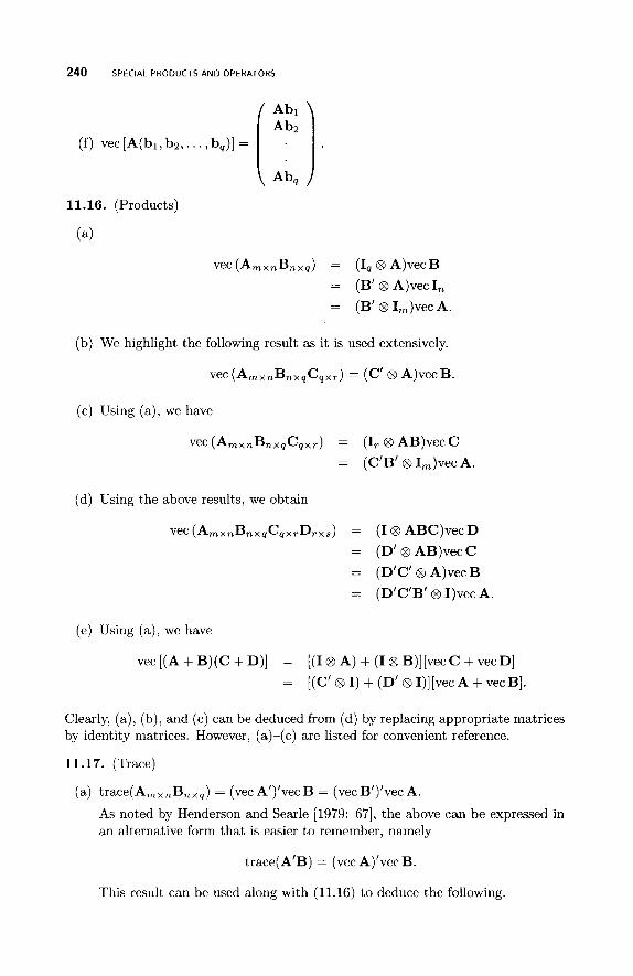
240 SPECIAL PRODUCTS AND OPERATORS
vec (AmxnBnxs) = (I, 8 A)vec B = (B’ 8 A)vec I,
= (B’ 8 1,)vec A.
(b) We highlight the following result as it is used extensively.
vec ( A m x n B n x q C q x r ) = (C’ 8 A)vecB
(c) Using (a), we have
VeC (AmxnBnxqCqxr) = (I, 8 AB)vecC = (C’B’ 8 1,)vec A.
(d) Using the above results, we obtain
vec (A,x,B,,,C,,,D,,,) = (I 8 ABC)vecD
= (D’ 8 AB)vec C
= (D’C’ 8 A)vec B
= (D’C’B’ 8 1)vec A.
(e) Using (a), we have
vec [(A + B ) ( C + D)] = [(I 8 A) + (I 8 B)] [vec C + vec D] = [ ( C ’ B I ) + (D’@~I) ] [vecA+vecB] .
Clearly, (a), (b), and (c) can be deduced from (d) by replacing appropriate matrices by identity matrices. However, (a)-(c) are listed for convenient reference.
11.17. (Trace)
(a) trace(AmxnBnxq) = (vecA’)’vecB = (vecB’)’vecA
As noted by Henderson and Searle [1979: 671, the above can be expressed in an alternative form that is easier to remember, namely
trace(A’B) = (vec A)’vec B.
This result can be used along with (11.16) to deduce the following.
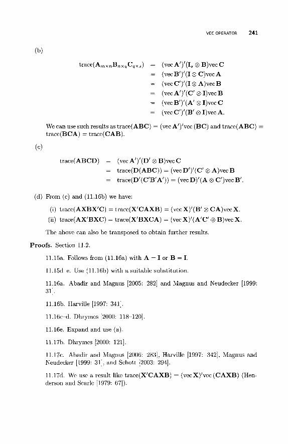
VEC OPERATOR 241
trace(A,x,B,xqCqx,) = (vec A’)’(Is @ B)vec C =
=
=
=
=
We can use such results as trace(ABC) = (vec A’)’vec (BC) and trace(ABC) = trace(BCA) = trace(CAB).
(vec B’)’(I 8 C)vec A (vec C’)’(I 8 A)vec B
(vec A’)’(,’ @ 1)vec B (vec .’)’(A’ 8 1)vec C (vec C’)’(B’ @ 1)vec A.
trace(ABCD) = (vec A’)’(,’ @ B)vec C =
=
trace(D(ABC)) = (vec D‘)’(C’ 8 A)vec B
trace(D’(C’B’A’)) = (vec D)’(A @ C’)vecB’.
(d) From (c) and (11.16b) we have:
(i) trace(AXBX’C) = trace(X’CAXB) = (vec X)’(B’ @ CA)vec X.
(ii) trace(AX’BXC) = trace(X’BXCA) = (vec X)’(A’C’ 8 B)vec X.
The above can also be transposed to obtain further results.
Proofs. Section 11.2.
11.15a. Follows from (11.16a) with A = I or B = I .
11.15d-e. Use (11.16b) with a suitable substitution.
11.16a. Abadir and Magnus [2005: 2821 and Magnus and Neudecker [1999: 311.
11.16b. Harville [1997: 3411.
11.16~-d. Dhrymes [2000: 118-1201.
11.16e. Expand and use (a).
11.17b. Dhrymes [2000: 1211
11.17~. Abadir and Magnus [2006: 2831, Harville [1997: 3421, Magnus and Neudecker [1999: 311, and Schott [2003: 2941.
11.17d. We use a result like trace(X’CAXB) = (vecX)’vec (CAXB) (Hen- derson and Searle [1979: 671).
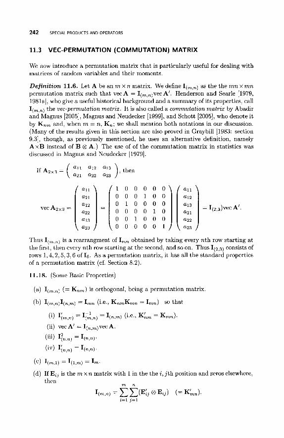
242 SPECIAL PRODUCTS AND OPERATORS
11.3 VEC- P E R M U TAT I 0 N (CO M M UTAT I0 N ) MATRIX
We now introduce a permutation matrix that is particularly useful for dealing with matrices of random variables and their moments.
Definition 11.6. Let A be an m x n matrix. We define I(,,+) as the the m n x m n permutation matrix such that vec A = I(,,,)vec A'. Henderson and Searle [1979, 198la], who give a useful historical background and a summary of its properties, call I(,,+) the uec-permutation matrix. It is also called a commutation matrix by Abadir and Magnus [2005], Magnus and Neudecker [1999], and Schott [2005], who denote it by K,, and, when m = n, Kn; we shall mention both notations in our discussion. (Many of the results given in this section are also proved in Graybill [1983: section 9.31, though, as previously mentioned, he uses an alternative definition, namely A x B instead of B @ A.) The use of of the commutation matrix in statistics was discussed in Magnus and Neudecker [ 19791.
1 0 0 0 0 0
= Ip3)vec A'. 0 0 0 0 1 0
a13 0 0 1 0 0 0
vecAzx3 =
a23 0 0 0 0 0 1 a23
Thus I(m,rL) is a rearrangment of I,, obtained by taking every nth row starting at the first, then every nth row starting at the second, and so on. Thus 1(2,3) consists of rows 1,4,2,5,3,6 of 16. As a permutation matrix, it has all the standard properties of a permutation matrix (cf. Section 8.2).
11.18. (Sonie Basic Properties)
(a) I(,,n) (= Knm) is orthogonal, being a permutation matrix.
z = 1 j=1
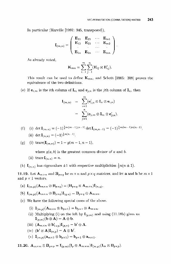
VEC-PERMUTATION (COMMUTATION) MATRIX 243
In particular (Harville [1997: 345, transposed]),
As already noted, m n
This result can be used to define K,,, and Schott [2005: 3081 proves the equivalence of the two definitions.
(e) If ei,, is the i th column of I, and ej, , is the j t h column of I,, then
m
I(m,n) C(ei,, @ 1, @ ei,,) i=l n
= C(ej., @ I, @ ei,n). j=1
where g(a, b) is the greatest common divisor of a and b.
(ii) trace I(,,,) = n.
(h) I(,,n) has eigenvalues fl with respective multiplicities in (n f 1).
11.19. Let A,,, and Bpxq be m x n and p x q matrices, and let a and b be m x 1 and p x 1 vectors.
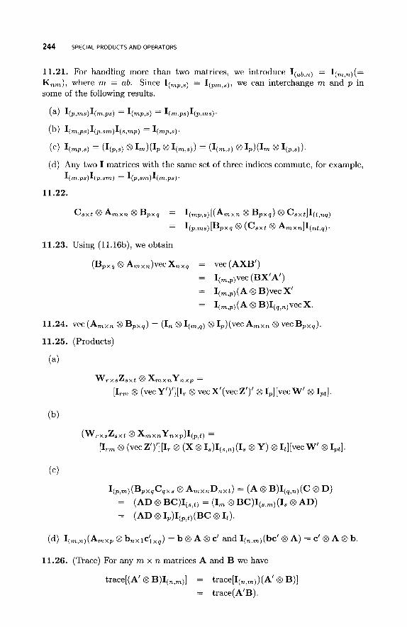
244 SPECIAL PRODUCTS AND OPERATORS
11.21. For handling more than two matrices, we introduce I (ab ,n ) = I(m,n)(= K,,), where m = ab. Since = we can interchange m and p in some of the following results.
(d) I (m,n)(Amxp 8 bnxlcixq) = b @ A €3 c’ and I(n.m)(bc’ €3 A ) = c’ @ A €3 b .
11.26. (Trace) For any m x n matrices A and B we have
trace[(A’ @ B)I(n,m)] = trace[I(,,,))(A’ @ B)] = trace(A’B).
244 SPECIAL PRODUCTS AND OPERATORS
( 4 I(p,ms)I(m,ps) = I(mp,s) = I(m,ps)I(p,ms).
(b) I(m,Ps)I(P,sm)I(s,mP) - I(mp,s) ’
(c) I(rnP,S) = (I(,,s) €3 Im)(Ip @ I (m,s)) = (I(m,s) @ I p ) ( I m 8 I(,$)).
-
(d) Any two I matrices with the same set of three indices commute, for example,
I ( ~ > P S ) I ( P > 4 = I(P,sm)I(m,Ps).
11.22.
C s x t €3 Am,, @ B p x q = I(mp,s)[(Amxn 8 B p x q ) €3 c s x t ] I ( t , n q )
I ( , , m s ) P p x q 8 (Csxt @ Amxnlqn t ,q ) . - -
11.23. Using (l l . l6b), we obtain
(Bpxq €3 Amxn)vecXnxq = vec (AXB’) = I(,,,)vec (BX’A‘)
- I(m,,) ( A €3 B)vec X’ -
= I(m,p)(A @ B)I(,,,)vecX.
11.24. vec (Amxn 8 BpXq) = (I, @ I(m,q) 8 Ip)(vecAmX, 8 vecBpxq).
11.25. (Products)
( 4
WrxsZsxt €3 X m x n Y n x p =
[Irm @ (vec Y’)‘][Ir €3 vec X’(vec Z’)’ 8 Ip][vec W’ €3 I,~].
GENERALIZED VEC-PERMUTATION MATRIX 245
Proofs. Section 11.3.
11.18. For proofs see Magnus [1988: chapter 31 and Magnus and Neudecker [ 19791. Also some proofs are given by Abadir and Magnus [2005: section 11.11, Harville [1997: section 16.31, Harville [2001: 149-1531, Magnus and Neudecker [1999: 471, and Schott [2005: 306-307, 3101.
11.19. Abadir and Magnus [2005: 3011, Harville [1997: 347-3481, and Schott [2005: 3081.
11.20. Use ( A @ Ip)(Im @ B) = A @ B and (11.19b).
11.21. Abadir and Magnus [2005: 3061 and Henderson and Searle [1981a: 284-2851.
11.22. Henderson and Searle [1981a: 2841 and Magnus [1988: 441.
11.23. Henderson and Searle [1981a: 2811 and Magnus [1988: 441.
11.24. Harville [1997: 3491, Magnus [1988: 431, and Schott [2005: 3091.
11.25a- b. Rogers [1980: 231
11.25~-d. Abadir and Magnus [2005: 302, 3041.
11.26. Abadir and Magnus [2005: 3041.
11.4 G E N ERA L I Z E D VEC- P E R M U TAT I0 N MATRIX
Definition 11.7. Let I(n) be the matrix obtained from I, by taking every n th row starting with the first, then every nth row starting with the second, and so on (cf. Tracey and Dwyer [1969] and Henderson and Searle [198la]). Then I(n) is called a generalized uec-permutation matrix. For example, if r = 5 and n = 3, I(3) = (el, e 4 , e2, e5, es) , where the ei are the columns of I,.
We can apply the same procedure to any matrix M and obtain M(n). In fact, M(n) = I(n)M. We can also define M(m,n) = I(m,n)M. When r = mn, I(m,n) = I(n), and when M has m n rows, M(m,n) = M(nl .
11.27. In the following, A is m x n , B is p x q, C is s x t , a is m x 1, and b is p x 1.
(a) vecA = (vecA’)(,,,).
(b) ( A @ B)(rn,P) = (B’ @ A’)(q,n).
(c) (a @ B)(rn,p) = I(m,n)(a @ B) = B @ a.
(4 ( A 8 b)(qp) = q m J ? ) ( A @ b) = b @ A.
(e) (a @ b)(m,p) = I ( m , p ) b @ b) = b @ a.
(f) (a @ b’ @ C),,, ,) = (ab’ 8 C), , , , ) = b’ €3 C 8 a.
11-28. I(rn,n) = (1, @ In) (m,n) .
246 SPECIAL PRODUCTS AND OPERATORS
Proofs. Section 11.4.
11.27. Henderson and Searle [1981a: 283-284 and equation (49)]. Use (1l.lb) for ( f ) .
11.5 VECH OPERATOR
Definition 11.8. If A is an n x n matrix, then vechA (vector-half) is the k = n(n+ 1)/2 -dimensional vector obtained by stacking the columns of the lower triangle of A, including the diagonal, one below the other; Magnus and Neudecker [1999] and Schott [2005] use the notation v(A). For example, if
all a12 a13
is symmetric, then all
vechA= [ 1. This approach is useful for symmetric and lower-triangular matrices; for upper- triangular matrices we use vech (A').
11.5.1 Symmetric Matrix
A major application of the above definition is to symmetric matrices, so we now assume A = A'. For this case, vechA lists all the distinct elements of A. As the elements of vec A are those of vech A with some repetitions, it follows that vec A and vechA are linear transformations of one another. This leads to the following definitions.
Definition 11.9. We have vech A = H, vec A and vec A = G, vech A. The matrix H, is k x n2, and Magnus and Neudecker [1999: 48-51] call the n2 x k matrix G, the duplication matrix D, (see also Magnus [1988: chapter 41 and Schott [2005: section 8.71). We shall also use the term duplication matrix. Examples of G, and H, for n = 3 ( k = 6) together with I(3,3), with which they have several relationships, are
D3 = G3(9 x 6) =
1 . . . . . I . . . . . I . .
' 1 ' . . 1 ' . 1 .
. . .
. . .
1 . ' . . . . 1 .
1
. .
. . . . .
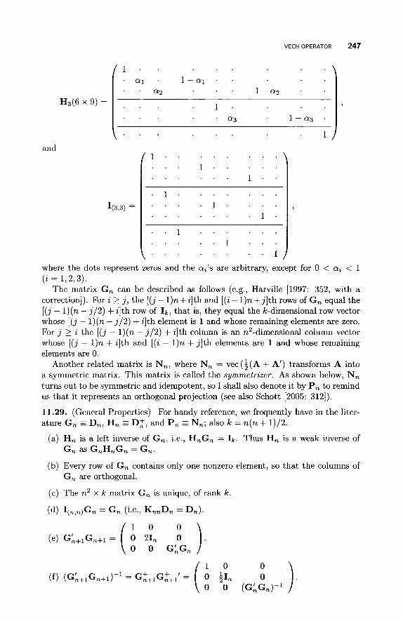
VECH OPERATOR
H3(6 x 9) =
and
’ 1 ’ . . . . . . ’ a 3 ’ 1-Ly3 .
. . ‘ 1 . . .
I(3,3) =
247
I
where the dots represent zeros and the ails are arbitrary, except for 0 < a!i < 1 (i = 1,2,3).
The matrix G, can be described as follows (e.g., Harville [1997: 352, with a correction]). For i 2 j , the [ ( j - l )n+i ] th and [(i - l ) n + j ] t h rows of G, equal the [ ( j - l ) (n - j /2) + i]th row of Ik, that is, they equal the k-dimensional row vector whose [ ( j - l ) (n - j / 2 ) + i]th element is 1 and whose remaining elements are zero. For j 2 i the [ ( j - 1)(n - j / 2 ) + i]th column is an n2-dimensional column vector whose [ ( j - 1). + 21th and [(i - 1)n + j l th elements are 1 and whose remaining elements are 0.
Another related matrix is N,, where N, = vec (;(A + A’) transforms A into a symmetric matrix. This matrix is called the symmetrizer. As shown below, N, turns out to be symmetric and idempotent, so I shall also denote it by P, to remind us that it represents an orthogonal projection (see also Schott [2005: 3121).
11.29. (General Properties) For handy reference, we frequently have in the liter- ature G, = D,, H, = Dk, and P, = N,; also k = n(n + 1)/2.
(a) H, is a left inverse of G,, i.e., H,G, = Ik. Thus H, is a weak inverse of G, as G,H,G, = G,.
(b) Every row of G, contains only one nonzero element, so that the columns of
(c) The n2 x k matrix G, is unique, of rank k .
(d) I(,,,)G, = G, (i..., K,,D, = Dn).
G, are orthogonal.
0 0 (el GL+,Gn+1= ( E 2: G;G, ) .
0 ( f ) (G;+~G,+I) -~ = G:+lG:+l’ = 0 ;I, 0 ( b 1 (GLG,)-’
248 SPECIAL PRODUCTS AND OPERATORS
(g) The k x n2 matrix H, is not unique and has rank k .
(h) A useful form of H, is H, = GR = (GLG,)-’GL, the Moore-Penrose inverse of G, (Schott [2005: 3131). (This is the form taken by H3(6 x 9) above when all the cq’s are set equal t o i.) Then:
(i) GRG, = I k .
(ii) G,G: = i(I,z + I(,,,))(= P,).
(iii) G,fI(,,,) = G,f.
( i ) P, = G,G: = G,(GkG,)-’G,. Then:
(i) P,G, = G, and GRP, = GR.
(ii) P,vecA = vec [$(A + A’)] for any n x n matrix A.
(iii) The symmetrizer P, is symmetric and idempotent, that is, a projection
(iv) rankP, = traceP, = in (n + 1).
matrix projecting orthogonally onto C(G,).
(v) P,I(,,%) = P, = I(,,,$’, (i.e., N,K,, = N, = K,,N,).
(vi) If A and B are n x n, then P,(A @ B)P, = P,(B @ A)P, and P,(A @ A)P, = P,(A 8 A) = ( A @ A)P,.
For further properties of G,, GL, GR, GLG,, and G,GL, where G, = D,, see Abadir and Magnus [2005: section 11.31 and Magnus [1988: chapter 41.
11.30. Suppose A and X are both n x n, and X is symmetric, then
vech(AXA’) = H,vec(AXA)
= H ( A @ A ) v e c X
= H,(A 8 A)G,vechX
= CvechX, say.
Properties of C are given in (11.31~) below.
11.31. Suppose A is n x n. Then:
(a) G,G,f(A @ A)G, = ( A @ A)G,.
(b) G,GR(A @ A)GR’ = (A @ A)GR’.
(c) Let C = H,(A @ A)G,, a k x k matrix, where k = n(n + 1)/2. Then:
(i) C is invariant with respect to the choice of H,, so we can choose H = G+
(ii) C is nonsingular if and only if A is nonsingular. Then
(cf. 11.29h).
c-l= G;(A-’ @ A-’)G,
(iii) If A is upper-triangular, lower-triangular, or diagonal, then C is re- spectively upper-triangular, lower-triangular, or diagonal with diagonal elements azzalj , i = 1 ,2 , . . . , n; j = 1 ,2 , . . . , n.
VECH OPERATOR 249
(iv) The eigenvalues of C are X i X j (1 5 j 5 i 5 n), where X i ( i = 1 , 2 , . . . , n)
(v) det C = det[G,f(A 8 A)G,] = (det A)"+1.
(vi) traceC = $[(traceA)2 + trace(A2)].
(vii) rankC = i[(rankA)2 +rankA].
(viii) C- = H,(A- 8 A-)G, is a weak inverse of C.
are the eigenvalues of A.
(d) If A is nonsingular, then:
(i) [GL(A 8 A)G,]-' = Gf(A- ' 8 A-')G:'.
(ii) det[G,f(A 8 A)G,f'] = 2Tn(,- ')/'(det A)"+'.
11.32. If A is any n x n matrix, then the following hold.
(a) (A 8 A)Gn = G,H,(A 8 A)G,.
(b) G,H,(A 8 A) = (A 8 A)G,H,.
(c) H,(A 8 A) = H,(A 8 A)G,H,.
We can set H, = G,f in the above.
For some properties of Gf(1, 8 A + A 8 I,)G,, G,f(A 8 B)G,, and some related matrices (with D, = G,), including further relationships between Dn+l and D,, see Magnus [1988: 65-72].
Proofs. Section 11.5.1.
11.29a. vechA = H, vecA = H,G,vechA for all symmetric A. Henderson and Searle [1979: 691.
11.29b. Follows from the definition of G,.
11.29~. Schott [2005: 3131
11.29d. Henderson and Searle [1979: 691
11.29e. Harville [1997: 3551, Magnus [1988: 721, and Magnus and Neudecker [1999: 511.
11.29f. Magnus [1988: 721 and Magnus and Neudecker [1999: 511
11.29g. Henderson and Searle [1979: 691.
11.29h. Abadir and Magnus [2006: 312-3131, Harville [1997: 354-3571, and Magnus [1988: 561.
11.29i. Abadir and Magnus [2005: 3071, Magnus [1988: 48-49], and Schott [2005: 3121. For (v) see also Abadir and Magnus [2006: 3081 and Magnus and Neudecker [ 1999: 501.
11.31a-b. Abadir and Magnus [2006: 3151, Magnus [1988: chapter 31, and Magnus and Neudecker [ 1999: 49-50].
250 SPECIAL PRODUCTS AND OPERATORS
11.31c(i). Henderson and Searle [1979: 701
11.31c(ii). Abadir and Magnus [2006: 3151, Harville [1997: 3581, Magnus [1988: chapter 31, and Magnus and Neudecker [1999: 49-50].
11.3lc(iii). Magnus [1988: 631.
11.31c(iv). Magnus [1988: 641.
11.31c(v). Abadir and Magnus [2006: 3161, Harville [1997: 3621, Henderson and Searle [ 1979: 701, and Magnus [1988: 64-65].
11.31c(vi). Abadir and Magnus [2005: 3161, Harville [1997: 3581, and Magnus [1988: 641.
11.31c(vii)-(viii). Harville [1997: 3581.
11.31d. Abadir and Magnus [2005: 3171, Magnus [1988: 651, and Schott [2005: 3151.
11.32. Harville [1997: 3581 and Henderson and Searle [1979: 701.
11.5.2 Lower-Triangular Matrix
Definition 11.10. Let A be an n x n lower-triangular matrix. If k = n(n + 1)/2, the k x n2 matrix L, is called the elimination matrix if vec A = LLvech A. The difference between G, and LL is that vecA now contains some zeros. Thus LL can be obtained from G, (= D,) by replacing n(n - 1)/2 rows of G, by zeros; (d) below gives a clearer picture.
11.33. We have the following properties for L,.
(a) L, has full row rank k.
(b) LLL = I k .
(c) L,f = Lk.
(d) From (b) we have vechA = L,vecA, so that L, eliminates the zeros from vec A.
(e) L,G, = I k , k = n(n + 1)/2.
( f ) G,L,P, = P,, where P, = ;(I,Z + I(,,,)) (i.e., D,L,N, = N,).
(g) G t = LP,.
Similar properties apply to the situation where A is strictly lower-triangular, that is lower-triangular but with zero diagonal elements (Schott 2005: 317-3181), Tri- angular matrices, and in fact any patterned matrix can be handled using a general kind of vec operator (cf. Section 18.3.5).
Proofs. Section 11.5.2.
11.33. Magnus [1988: 77, 801 and Schott [2005: 316-3171
STAR OPERATOR 251
11.6 STAR OPERATOR
Definition 11.11. Let A = (aij) be m x n and B be mp x nq . Then we define the p x q matrix (MacRae [1974])
m ri
A * B = 7; aijBij, i=l j=1
where Bij is the ( i , j ) th submatrix of B when B is partitioned into submatrices of size p x q. When A and B are the same size, A * B = trace(A’B).
11.34. If C is r x s, then (A * B ) @ C = A * (B €3 C).
11.35. A * B = B * ( A @ vecI,(vecI,)’).
11.36. If x is p x 1 and y is q x 1, then
x’(A * B)y =
=
A * (I, @ x’)B(I, €3 y)
(I, @ x)A(I, €3 y’) * B.
11.37.
XmxnYnxpZpxq = Y * vecX(vecZ’)’ = Y’ * (Z €3 I,)I(,,q)(x €3 Iq).
Proofs. Section 11.6.
11.34-11.37. MacRae [1974].
11.7 H A D A M A R D PRODUCT
We now consider a particular product that arises in a wide variety of mathematical applications such as covariance matrices for independent zero mean random vectors and characteristic functions in probability theory (Horn and Johnson [1985: 301, 393-3941). Further mathematical applications are described by Horn and Johnson [1985: 455-4571 and Horn and Johnson [1991: chapter 51. The Hadamard product appears in several places in this book. In this section A t B means that A - B is non-negative definite.
Definition 11.12. If A = (azJ) and B = ( b t J ) are m x n real or complex matrices, then their Hadamard product (also referred to as the Schur product) is the m x n matrix A o B = (at3bt3). The results below, where proofs are not referenced, follow from the definition by simply multiplying out the appropriate matrices.
11.38. Let A and B be m x n matrices, and let e, be the i th column of I,.
(a) Let am = Eyll ei(ei @ e,)’ = CzI e,(vecEii)’, where Eii = eiel,. Then:
(i) A o B = @,(A €3 B)@L.
252 SPECIAL PRODUCTS AND OPERATORS
(ii) @,@k = I,.
(iii) If C = ( c z j ) is m x m, then
@,vecC = (c~I,cz~,~~~,c,,)’ = (diagC)l,.
(iv) @,I(,,,) = 9,.
(b) A o B is a submatrix of A @ B. In fact
A 0 B = (A @ B),,p,
where (a , p) denotes the submatrix formed by the intersection of the rows of A @ B in Q with the columns in /3, where Q = { 1, m + 2,2m + 3, . . . , m2} and p = { l , n + 2 , 2 n + 3 , . . . , n’}.
(c) If m = n, then A o B is a principal submatrix of A @ B.
The above results can be used to prove results about A o B using A @ B
11.39. Let A and B be m x n matrices. Then the following hold.
(a) A o B = B o A
(b) ( A o B)’ = A’ o B’.
(c) trace(AB’) = 1A(A o B)ln.
(d) rank(A o B) 5 rankA . rankB.
11.40. If all matrices are the same size, then
(A + B) o (C + D) = A o C + A o D + B o C + B O D .
11.41. If A , B, and C are all m x n matrices, then
trace[(A o B)C’] = trace[(A o C)B’].
11.42. (Multiplication by Diagonal Matrices) Suppose A and B are m x n, D is m x m, and E is n x n, where D and E are diagonal matrices, then
D ( A o B)E = (DAE) o B = (DA) o (BE) = (AE) o (DB) = A o (DBE).
11.43. If A is square, then A o 11’ = A = 11’ o A .
11.44. (Quadratics) Then
Let A and B be n x n matrices, and suppose y , z E C”.
y”(A o B)z = trace(D;AD,B’),
where D, = diag(y) and D, = diag(z).
11.45. If A and B are Hermitian matrices. then so is A o B.
11.46. Let A and B be Hermitian non-negative definite n x n matrices, that is, A k 0 and B 0. Then:
(a) A o B 5 0. The same results apply to A o A 0 . . . o A to any number of terms.
HADAMARD PRODUCT 253
(b) det(A o B) + det A . det B 2 b l l b z z . . . b,, det A + u11u22 . . . a,, det B.
(c) ~ a z 2 b z 2 2 d e t ( A o B ) 2 bllbzz...b,,detA 2 d e t A d e t B . n
2=1 (Note that A and B can be interchanged.) The left-hand side follows from (12.27).
(d) A2 o B2 h (A o B)'.
(e) If A and B are positive definite, then:
(i) A o B is positive definite.
(ii) A-' o B-' k ( A o B)-'.
( f ) If A + 0, and B k 0 with T nonzero diagonal entries, then rank(A o B) = T .
(g) If B + 0, and A 5 0 with positive diagonal elements, then A o B + 0.
(h If A + 0, then A o A-' I, 2 (Ap' o A)-'. Horn and Johnson [1991: section 5.41 discuss the properties of A o A-l and A o (A-l)'.
11.47. (Fejer's Theorem) Let A be any n x n matrix. Then A is Hermitian non- negative definite if and only if trace(A o B) 2 0 for all Hermitian non-negative definite n x n matrices B.
11.48. (Eigenvalues) matrices.
Let A and B be n x n Hermitian non-negative definite
(a) Let bmaX and bmin be maximum and minimum entries of the diagonal elements of B. Then, for all j,
brninXrnin(A) I XJ(AoB) I bmaxXmax(A).
(b) Amin(A)Xmin(B) I Xj(AoB) I Arnax(A)Amax(B) for all j .
(c) Let R = ( p z j ) be any n x n correlation matrix.
( i ) Since p2i = 1 for all i, it follows from (a) that
(ii) Setting R = I, we have Xmin(A) I ~ j j I xrnax(A)
Xmin(A) I Aj(AoR) I &nax(A).
(d) Xmin(A 0 B) 2 Xrnin(AB).
11.49. (Singular Values) Let A and B be m x n matrices, and let nJ(C) be the j t h singular value of C , where the singular values are listed in decreasing order of magnitude. Then
2 2
C n J ( ~ o ~ ) I ~ ~ ~ ( A ) ~ ~ ( B ) , i = i , 2 , . . . , n. J=1 J = 1
11.50. If A and B are real or complex m x n matrices, then
(AA') o (BB*) 5 ( A o B)(A* o B*)
254 SPECIAL PRODUCTS AND OPERATORS
11.51. Let A and B be n x n Hermitian positive definite matrices, and let C and D be any m x n real or complex matrices. Then
(CA-lC*) o (DB-lD*) (C o D)(A o B)-’(C o D)*.
Proofs. Section 11.7.
11.38a. Magnus [1988: 1101 and Schott [2005: 297, (i)] .
11.38b-c. Horn and Johnson [1991: 3041.
11.39. Here (a) and (b) are obvious, (c) and (d) are given by Schott [2005: 2971, and (d) is given by Horn and Johnson [1991: 3071.
11.40. Follows directly from the definition of “0 ” .
11.41. Horn and Johnson [1991: 305-3061.
11.42. Let C = A o B. Then (DCE),, = c, ~,di,c,,e,j, which can be expressed in the form C, C, di,arsesj . b,, = [(DAE) o B]ij, and so on.
11.43. Follows from aij . 1 = aij.
11.44. Horn and Johnson [1991: 3061 and Schott [2005: 2981
11.46a. Horn and Johnson [1985: 4581, Rao and Rao [1998: 204, 2151, Schott [2005: 299, real case], and Zhang [1999: 1921.
11.46b. Rao and Rao [1998: 2121.
11.46~. Rao and Rao [1998: 2101, Schott [2005: 3021, and Zhang [1999: 2001.
11.46d. Zhang [1999: 193)
11.46e(i). Abadir and Magnus [2005: 3401 and Rao and Rao [1998: 2041.
11.46e(ii). Horn and Johnson [1985: 4751 and Zhang [1999: 1931.
11.46f. Rao and Rao [1998: 2131.
11.46g. Horn and Johnson [1991: 3091 and Schott [2005: 300, real case].
11.46h. Horn and Johnson [1985: 4751, Schott [2005: 3041, and Zhang [1999: 1931.
11.47. Rao and Rao [1998: 2141.
11.48a. Rao and Rao [1998: 2061 and Schott [2005: 303, real case].
11.48b. Horn and Johnson [1991: 3121 and Rao and Rao [1998: 2071.
11.48~. Rao and Rao [1998: 2071.
11.48d. Bapat and Raghavan [1997: 142, real case] and Schott [2005: 305, real case].
11.49. Horn and Johnson [1991: 3341.
11.50. Zhang [1999: 1941.
11.51. Zhang [1999: 1981.
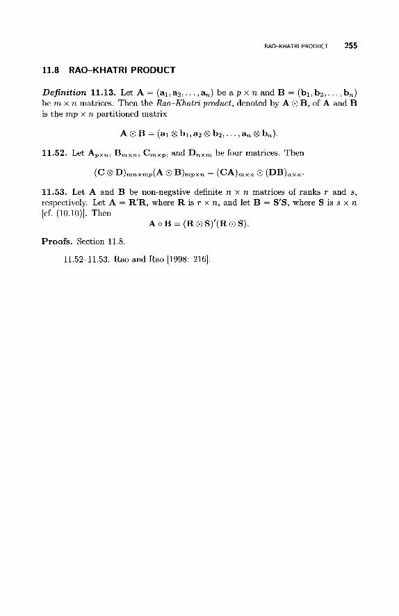
RAO-KHATRI PRODUCT 255
11.8 RAO-KHATRI PRODUCT
Definition 11.13. Let A = (al, a 2 , . . . ,a,) be a p x n and B = (bl, b2,. . . , b,) be m x n matrices. Then the Rao-Khatri product, denoted by A 0 B, of A and B is the m p x n partitioned matrix
A O B = (a1 C3 bl,a2 8 b2,. . . ,a, 8 bn).
11.52. Let Apxn, B,,,, Cmxpr and D,,, be four matrices. Then
( C 8 D)mnxmp(A O B ) m p x n = (CA)mxn O (DB)nxn.
11.53. Let A and B be non-negative definite n x n matrices of ranks r and s, respectively. Let A = R’R, where R is r x n, and let B = S’S, where S is s x n [cf. (10.10)]. Then
A o B = (R 0 S)’(R 0 S ) .
Proofs. Section 11.8.
11.52-11.53. Rao and Rao [1998: 2161.

This Page Intentionally Left Blank
CHAPTER 12
IN EQUALlTl ES
Inequalities are used extensively in statistics and, because they relate t o almost every chapter in this book, they are difficult to categorize. Those concerned with general inner products and norms are considered in Sections 2.2.1 and 4.6. Those involved with ranks are discussed in Chapter 3, while those for eigenvalues appear in Chapter 6. Some inequalities for non-negative definite matrices appear in Chapter 9, and those relating to majorization appear in Chapter 23. There are a large number of inequalities involving probability and random variables and a selection of these appear in Chapters 22 and 23. Optimization in Chapter 24 generates further inequalities. So what is in this chapter? I have collected here some of the more traditional inequalities such as Cauchy-Schwarz, Kantorovich, Holder, Minkowski, and so on, and their extensions. At the end I have listed a few identities that can be useful in setting up inequalities.
1 2.1 C A U C H Y-S C H WA R Z I N EQUAL IT I ES
The inequalities given below are fairly basic ones. However, for further extensions and refinements, including those for complex numbers, the reader is referred to Dragomir [2004: chapters 1-31,
A Matrix Handbook for Statisticians. By George A. F. Seber Copyright @ 2008 John Wiley & Sons, Inc.
257
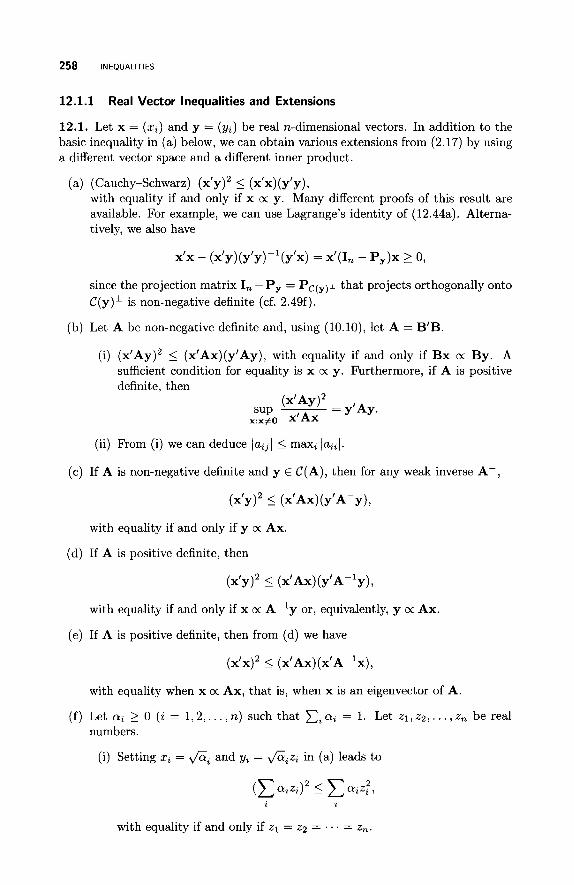
258 INEQUALITIES
12.1.1
12.1. Let x = (xi) and y = (yi) be real n-dimensional vectors. In addition to the basic inequality in (a) below, we can obtain various extensions from (2.17) by using a different vector space and a different inner product.
Real Vector Inequalities and Extensions
(a) (Cauchy-Schwarz) (x’Y)~ 5 (x’x)(y’y), with equality if and only if x 0: y. Many different proofs of this result are available. For example, we can use Lagrange’s identity of (12.44a). Alterna- tively, we also have
x’x - (x’y)(y’y)-’(y’x) = x’(1, - P,)x 2 0,
since the projection matrix I, - P, = P c ( y ) ~ that projects orthogonally onto C(y)’ is non-negative definite (cf. 2.49f).
(b) Let A be non-negative definite and, using (10.10), let A = B’B.
(i) ( x ’ A ~ ) ~ 5 (x’Ax)(y’Ay), with equality if and only if Bx K By. A sufficient condition for equality is x 0: y. Furthermore, if A is positive definite, then
(ii) From (i) we can deduce (aijl 5 maxi laii(.
(c) If A is non-negative definite and y E C(A), then for any weak inverse A-,
(X’YI2 I (x’Ax)(y’A-y),
with equality if and only if y 0: Ax.
(d) If A is positive definite, then
( x ’ Y ) ~ 5 (x’Ax)(Y’A-~Y),
with equality if and only if x 0: A-’y or, equivalently, y K Ax.
(e) If A is positive definite, then from (d) we have
(x’x)2 I ( x ’ ~ x ) ( x ’ ~ - l ~ ) ,
with equality when x 0: Ax, that is, when x is an eigenvector of A.
(f) Let ai 2 0 (i = 1 , 2 , . . . , n) such that xi cyi = 1. Let zl, z2,. . . , z, be real numbers.
(i) Setting xi = f i i and yi = f i i z i in (a) leads to
i i
with equality if and only if z1 = z2 = . . . = zn.
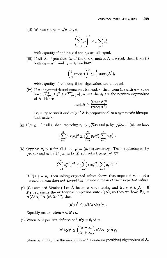
CAUCHY-SCHWARZ INEQUALITIES 259
(ii) We can set ai = 1/n to get
with equality if and only if the zis are all equal.
with ai = n-l and zi = Xi, we have (iii) If all the eigenvalues X i of the n x n matrix A are real, then, from (i)
1 (i trace A) 5 trace(A2),
with equality if and only if the eigenvalues are all equal.
have (C;=‘=, of A. Hence
(iv) If A is symmetric and nonzero with rank T , then, from (ii) with n = T , we 5 TC;=~ A:, where the A, are the nonzero eigenvalues
(trace A)2 trace(A2) .
rankA 2
Equality occurs if and only if A is proportional to a symmetric idempo- tent matrix.
(g) If p , 2 0 for all i, then, replacing 5, by f i x z and yz by fiy, in (a), we have
i = l i=l i=l
(h) Suppose z, > 0 for all i and p = ( p Z ) is arbitrary. Then, replacing 5, by &/pt and y, by 1/& in (a)(i) and rearranging, we get
n n n
a= 1 i = l i=l
If E(xi) = pi, then taking expected values shows that expected value of a harmonic mean does not exceed the harmonic mean of their expected values.
(i) (Constrained Version) Let A be an n x n matrix, and let y E C(A). If PA represents the orthogonal projection onto C(A), so that we have PA = A(A’A)-A (cf. 2.49f), then
(x’Y)2 5 (x’PAx)(y’y)
Equality occurs when y 0: PAX.
(j) When A is positive definite and x’y = 0, then
where X1 and An are the maximum and minimum (positive) eigenvalues of A.
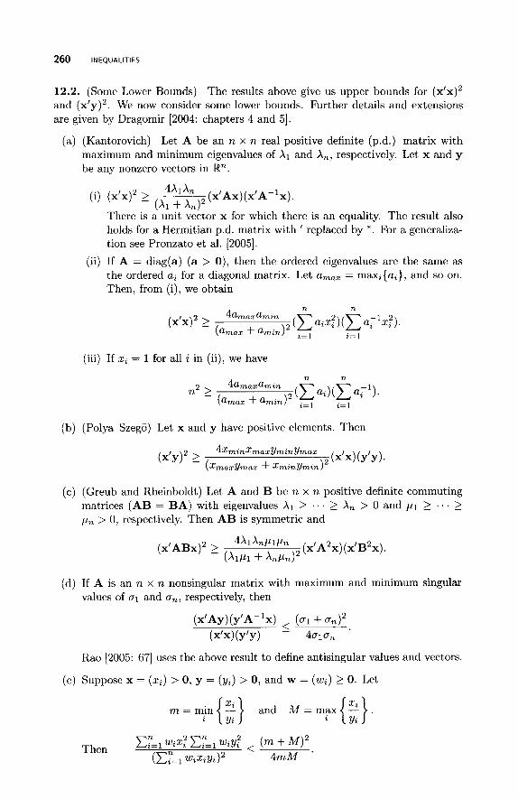
260 INEQUALITIES
12.2. (Some Lower Bounds) The results above give us upper bounds for (x’x)~ and (x’y)’. We now consider some lower bounds. Further details and extensions are given by Dragomir [2004: chapters 4 and 51.
(a) (Kantorovich) Let A be an n x n real positive definite (p.d.) matrix with maximum and minimum eigenvalues of A1 and A,, respectively. Let x and y be any nonzero vectors in B n .
There is a unit vector x for which there is an equality. The result also holds for a Hermitian p.d. matrix with ’ replaced by *. For a generaliza- tion see Pronzato et al. [2005].
(ii) If A = diag(a) (a > 0) , then the ordered eigenvalues are the same as the ordered ai for a diagonal matrix. Let amax = maxi{ai}, and so on. Then, from (i), we obtain
(iii) If xi = 1 for all i in (ii), we have
(b) (Polya-Szego) Let x and y have positive elements. Then
(x‘x) (Y‘Y 1. 4 x m i n ~ m a x ~ m z n ~ m a x
(xmaxymax + xminYmin)2 (X’YI2 L
(c) (Greub and Rheinboldt) Let A and B be n x n positive definite commuting matrices (AB = BA) with eigenvalues A1 2 . . . 2 An > 0 and p1 2 . . . 2 pn > 0, respectively. Then AB is symmetric and
(d) If A is an n x n nonsingular matrix with maximum and minimum singular values of 01 and on, respectively, then
(x’AY)(~’A-~x) (Q + I
(x’4 (Y’Y 1 4010,
Rao [2005: 671 uses the above result to define antisingular values and vectors.
(e) Suppose x = ( x i ) > 0, y = (yi) > 0, and w = (wi) 2 0. Let
m = min { z} and M = m a x { $}
CAUCHY-SCHWARZ INEQUALITIES 261
Proofs. Section 12.1.1.
12.la. Abadir and Magnus [2005: 71.
12.lb. Abadir and Magnus [2005: 3231.
1 2 . 1 ~ . Neudecker and Liu [1994: 3511. Use y'Ay = y'AA-Ay in (b)(i) and set z = Ay.
12.ld. Replace x by A1I2x and y by A-'12y in (a).
12.lf(iv). Abadir and Magnus [2005: 3241.
12.lh. Rao and Rao [1998: 4611.
12.li. Use (b) with A replaced by PA. If y 6 C(A), then y = PAY.
12.1j. Drury et al. [2002: 971.
12.2a. Abadir and Magnus [2005: 3311, Horn and Johnson [1985: 4441, Rao and Rao [1998: 4621, and Zhang [1999: 2041.
12.2b. Dragomir [2004: 931 and quoted by Rao and R m [1998: 4561.
1 2 . 2 ~ . Greub and Rheinbolt [1959] and quoted by Rao and Rao [1998: 4561.
12.2d. Strang [1960] and quoted by Rao and Rao [1998: 4651.
12.2e. Dragomir [2004: 911.
12.1.2 Complex Vector Inequalities
Many of the above inequalities can be generalized to the complex case. By the same token, the following results for complex vectors will hold for their real counterparts.
12.3. Let x and y be two complex vectors in C", and let A be a Hermitian non- negative definite n x n matrix.
(a) There are two versions of the Cauchy-Schwarz inequality.
(i) Using the inner product (x,y) = x*y, we have from (2.17) that
x*x - (x*y)(y*y)-l(y*x) L 0.
Equality occurs when x 0: y.
(ii) Since lab] = lallbl, we have from (5.lb),
i=l i=l i=l i= 1
Equality occurs when x = cy for any complex scalar c.
(b) 1x*yI2 5 (x*x)(y*y). Equality occurs when x 0: y.
262 INEQUALITIES
(c) (x*Ay12 5 (x*Ax)(y*Ay), with equality when x c( y.
(d) Let A be Hermitian positive definite.
(i) Ix*yI2 5 (x*Ax)(y*A-ly). Equality occurs when y c( Ax.
(ii) ( x * x ) ~ 5 (x*Ax)(x*A-lx), which implies (x*Ax)-' I x*A-lx when x*x = 1. Equality occurs when x 0: Ax, that is, when x is an eigenvec- tor.
( e ) (Wielandt) If A is Hermitian positive definite and x*y = 0, then
Equality occurs when x = (XI + x,)/& and y = (XI - x,)/&, where x1 and x, are the eigenvectors corresponding to A1 and A,, respectively, the maximum and minimum eigenvalues of A. Rao [2005: 631 applies the above result to sphericity tests in multivariate analysis. Along with references, he also gives a matrix generalization of the above result (Rao [2005: 621).
Note that I . I represents the modulus.
12.4. Let A and C be Hermitian positive definite n x n and m x m matrices, respectively, and let B be n x m. The following statements are equivalent:
(1) (x*Ax)(y*Cy) 2 Ix*By12 for all x E Cn and all y E C".
(2) x*Ax + y*Cy 2 2lx*Byl for all x E C" and all y E C".
(3) p(B*A-lBC-l) I 1, where p ( . ) is the spectral radius.
(4) ( ) 0 (i.e., non-negative definite).
Proofs. Section 12.1.2.
12.3. For (a) see Dragomir [2004: 2-31; for (a)-(d) see Zhang [1999: 2031 (and quoted by Rao and Rao [1998: 4551); and for (e), Horn and Johnson [1985] and Rao [2005: 61, real case].
12.4. Horn and Johnson [1985: 4731.
12.1.3 Real Matrix Inequalities
In this section we give a number of matrix inequalities that might be regarded as extensions of the Cauchy-Schwarz inequality for vectors.
12.5. Let A and B be any real m x n matrices.
(a) (traceA'B)2 5 (traceA'A)(traceB'B), with equality if and only if one of the matrices is a multiple of the other.
CAUCHY-SCHWARZ INEQUALITIES 263
This inequality can also be expressed in the form I(A,B)I 5 llAll~llBll~ (cf. (2.20) and Harville [1997: 62]), where 11 . I I F is the Frobenius norm. For some generalizations see Rao and Rao [ 1998: 494-4951.
trace[(A’B)’] 5 trace[(A’A)(B’B)], with equality if and only if AB’ is sym- metric. Furthermore, since trace(A’B) = trace(B’A) = trace(AB’), we have
trace[ (A’B)2] 5 trace[ ( AA’) (BB’)] ,
with equality if and only if A’B is symmetric.
Setting m = n and A = I,, we have
trace(B’) 5 trace(B’B),
with equality if and only if B is symmetric.
(det A’B)’ 5 (det A’A)(det B’B), with equality if and only if A’A or B‘B are singular, or if B = A R for some nonsingular R.
From (2.15a) we have IIA+BIIF 5 IIAIIF+~~BIIF, where 1 1 . 1 1 ~ is the Frobenius norm.
A’[I, - B(B’B)-B’]A = A’(1, - PB)A is non-negative definite since (I, - PB) is non-negative definite (cf. 2.49f). Hence, from (10.48b),
det (A’A) 2 det [A’B( B’B)-B’A].
12.6. (Measures of Relative Efficiency in Regression) Consider the linear regres- sion model of Section 20.7, namely y = X P + E , where X is n x p of rank p , var(e) = 02V, and V is positive definite. We define the eigenvalues of V to be Xi = Xi(V) and we impose the usual order X1 2 Xz 2 . . . 2 An > 0. Then the variance matrix of the generalized (weighted) least squares estimate of P is (X’V-’X)-’ and that of the ordinary least squares estimator is (X’X)-l(X’VX)(X’X)-’. Measures of the relative efficiency of the ordinary least squares estimate with respect to the generalized least squares estimate have been based on the roots of
det[(X’X)-l(X’VX)(X’X)-l - B(X’V-lX)-l] = 0.
Four such measures Ei (i = 1,2,3,4) taken from Rao and Rao [1998: 4641 are given below.
det(X’VX) det(X’V-lX) [det (X’X))]
= n 6%. If s = min{p, n - p } , then i=l
(a) El =
P
(b) Ez = XBi. If s = min{p,n - p } , t = 0 if s = p , and t = 2 p - n if s = n-p , i=l
then

264 INEQUALITIES
When X’X = I,,
s
0 L E3 5 E ( 6 - JG)’, i=l
where s = min{p, n - p } .
(d) Ed = trace[PV’P - ( P V P ) ( P V P ) ] , where P = X(X’X)-lX’ represents the orthogonal projection onto C(X). Then
12.7. (Matrix Kantorovich Inequality) Let A be a positive definite n x n matrix, and let U be an n x p matrix such that U’U = I,. If A1 = A,,,(A) and A, =
Arnin(A)> then U‘AU 3 (’1 + A,)2 (U/A-lU)-l .
4 k L
Interchanging A and A-’ so that A;’ = Amin(A-’) and A;’ = Amax(A-’), we have
U/A- lU 5 (’1 + A,)2 (U/AU)-l , 4hA,
Also (U’AU)-’ 3 U’A-’U.
(Note that B 5 C means that C-B is non-negative definite.) For further extensions see Baksalary and Puntanen [1991] and Drury et al. [2002].
12.8. (Further Matrix Kantorovich-Type Inequalities)
(a) Let A, B, and C be n x n positive definite matrices, and let X be an n x k matrix of rank k. Then:
(i)
det (X’B-‘ AB-’ X) det (X’ A-’ X ) [det (X’B-’ X)]’
(pi + pn-i+l)’ = 5 4PiP,-i+l ’ SUP
X
where m = min{k,n - k } and 11 2 . . . 2 p, > 0 are the roots of det(B - p A ) = 0, that is, the eigenvalues of BA-’ (and of A-’B).
(ii)
det(X’B2X) det(X’C2X) (pa + Pn-Z+d2
s:p [det (X’BCX)]’ =z 4,&Pn-i+1 ’
where m = min{k, n - k } , BC = CB, and the pi are the eigenvalues of BC-’.
CAUCHY-SCHWARZ INEQUALITIES 265
(b) Let B be an n x n non-negative definite matrix of rank b, and let A be n x T of rank u (u 5 min{b,r}) such that C(A) C C(B). Furthermore, let X1 2 . . . 2 Xb > 0 be the eigenvalues of B. Then, if A+ and B+ are Moore- Penrose inverses, we have:
with equality if and only if A = 0, or A‘BA = $ ( A 1 + Xb)A’A and A‘B+A = X l f X b ~ l ~
2X1Xb . (ii) A+B(A+)’ - (A’B+A)+ 5 (6 - &)’(A’A)+,
with equality if and only if A = 0, or X 1 = Xb, or A’BA = (XI + X b -
&&)A’A and A’B+A = (X1Xb)-1/2A’A.
The above, along with two further results, are quoted by Rao and Rao [1998: 4961. They also give a Kantorovich-type inequality for complex matrices. See also Liu [2002a] and Liu and Neudecker [1996].
Proofs. Section 12.1.3.
12.5a--b. Abadir and Magnus [2005: 3251 and Magnus and Neudecker [1999: 201-2021.
2011. 12 .5~ . Abadir and Magnus [2005: 3301 and Magnus and Neudecker [1999:
12.6a. Bloomfield and Watson [I9751 and Knott [1975].
12.6b. Khatri and Rao [1981, 19821.
12 .6~ . Rao [1985]; see also Drury et al. [2002: section 31 for further details and related work.
12.6d. Bloomfield and Watson [1975].
12.7. Marshall and Olkin [1990] and Zhang [1999: 2041.
12.8a(i). Lin [1984].
12.8a(ii). Khatri and Rao [1981]. This result follows from (i) by replacing A-’ by C2 and B-l by BC. Here BC is symmetric and positive definite when BC = CB as the eigenvalues of B1/2CB1/2 are positive.
12.1.4 Complex Matrix Inequalities
12.9. Let X and Y be n x p and n x q complex matrices, respectively. generalizing (12.5e), we have
Then
x*x - x*Y(Y*Y)-Y*x = X*(I, - Py)X 0,
i.e., non-negative definite as the orthogonal projector I, - Py is Hermitian non- negative definite (cf. 2.49f). Equality occurs if and only if C(X) C C(Y). A gener- alization of this result follows.
266 INEQUALITIES
12.10. Let A be an n x n Hermitian non-negative definite matrix with PA = A(A*A)-A*, and let U be an n x p matrix. Then
U * A + U h U*PAU(U*AU)+U*PAU,
with equality if and only if C(AU) = C(PAU)
12.11. Let A be an n x n Hermitian positive definite matrix, and let X be n x p and Y be n x q satisfying X*Y = 0. Then
where (Y*AY)- is any weak inverse, with equality when
(u1+ u,) K (A,1PUl + A,1Pu,).
Here P = X(X*X)-X* is the orthogonal projector onto C(X) and A1 and A, are the largest and smallest eigenvalues, respectively, of A with corresponding eigenvectors u1 and u,.
12.12. Let A and B be n x n real or complex matrices.
(a) I trace(AB)I2 I trace(A*A) trace(B*B).
(b) If A and B are Hermitian, then
t r a ~ e [ ( A B ) ~ ] 5 trace(A2B2),
with equality if and only if A B = B A . For a generalization see (12.33d).
12.13. (Unitarily Invariant Norm) Let 1 1 . ] I u , be any unitarily invariant norm defined on the vector space of m x n complex matrices (Section 4.6.3), and let A and B be m x n matrices.
(a) If IAl represents the general square root of A (i.e., [A/ = (A*A)l/'), then:
(i) II IA*BIP 112, I ll(A*A)pllUz Il(B*B)PIIUZ for all P > 0. (ii) Setting p = f in (i) and using 11 IAl l l u z = llAllUz (cf. 4.86), we have
II IA*Bl+ 112, I IlAlluz IlBllUZ.
IIA*BII:~ I I I A * A I I ~ ~ I IB*BII~ , .
(iii) If p = 1 in (i), we have a Cauchy-Schwarz type of inequality
(b) (Hadamard Product) IIA o B112, 5 IIAA*(),, ~ ~ B * B ~ ~ u , .
Proofs. Section 12.1.4.
12.10. Baksalary and Puntanen [1991: 1041, who also give some special cases and variations on the result.
12.11. Wang and Ip [2000] (see also Drury [2002]).
12.12. Zhang [1999: 25, 2131.
12.13a. Horn and Johnson [1985: 212, exercises 6 and 7, hint for proof only].
12.13b. Horn and Johnson [1991: 212, exercise 8, hint for proof only].
HOLDER,S INEQUALITY AND EXTENSIONS 267
12.2 HOLDER'S INEQUALITY AND EXTENSIONS
Let a, b, . . . , g be m real n x 1 vectors of non-negative elements, and let a i > 0 ( i = 1 , 2 , . . . ,n ) such that C z l 01i = 1.
12.14. n n n n
n a y . + n b ; t + . . . + ngz" . 5 H ( a , + bi + . . . + g p . i= 1 i= 1 i=l i=l
Equality occurs if and only if either every pair of vectors a, b, and so on, are proportional, or there is a k such that a k = bk = . . . = gk = 0. If A = (a, b, . . . , g ) , then the conditions for equality are either rank A = 1 or A contains a row of zeros.
12.15. Interchanging the rows and columns of A in the previous result leads to the following.
n n n
2=1 a=1 z= 1 a = 1
with equality if and only if rankA = 1 or A contains a column of zeros.
Putting m = 2 in (a) leads to
n n n
2= 1 i=l
with equality if and only if a = k b .
(Holder's Inequality) Replacing ai by a,"" and b, by b:'(l-a) in (b) leads to
n n n
i=l i=l i=l
i=l i=l
where T ( = 1/01) > 1 and r P 1 + s-l = 1. Equality occurs if and only if a: = kbp for i = 1 , 2 , . . . , n, or either a or b is 0. The inequality in (c) is reversed if T # 0, T < 1 (and s < 0). We can deduce the previous results from
(c).
If a and b are vectors of complex numbers, then replacing ai by lail, and so on, in (c), we have for T > 1 and T - ~ + s-l = 1,
n n n
i=l i= 1 i= 1
Equality occurs if and only if
for i = 1 , 2 , . . . , n, and arg(aibi) is independent of i .
268 INEQUALITIES
12.16. (Matrix Analogues) Let A and B any two n x n non-negative definite matrices, and let 0 < Q < 1.
(a) (Magnus) trace(AaBlPa) I (traceA)a(traceB)'-a
with equality if and only if B = kA for some k > 0.
(b) trace(AaB1-") 5 trace[aA + (1 - a)B]
with equality if and only if A = B.
(c) (det A)"(det B)lPa I det(aA + (1 - a)B)
with equality if and only if A = B or det(aA + (1 - a)B) = 0. The re- sult is obviously true if either A or B is singular, so it is more applicable to positive definite matrices. In this case it follows that +(A) = log det A is concave on the space of positive definite matrices.
(d) Let Ai be positive definite and ai > 0 for (i = 1 , 2 , . . . , k ) , where Ci ai = 1. Then
(det A I ) ~ ~ (det A2)az . . . (det At)ak I det(alA1 + a2Az + . . . + akAt),
with equality if and only if the Ai are all equal.
Proofs. Section 12.2.
12.14. Hardy et al. [1952: section 2.71 and Magnus and Neudecker [1999: 220-2211,
12.15~. For a direct proof see, for example, Marcus and Minc [1964: 1081, Rao and Bhimasankaram [2000: 2541, and Rao and Rao [1998: 4571.
12.16a. Magnus and Neudecker [1999: 2211.
12.16b. Magnus and Neudecker [1999: 2221.
12.16~. Abadir and Magnus [2005: 3341 and Magnus and Neudecker [1999: 2221.
12.16d. Abadir and Magnus [2005: 334-3351,
12.3 MINKOWSKI'S INEQUALITY AND EXTENSIONS
12.17. Let X be an m x n real matrix whose elements are non-negative and not all zero. If p > 1, then
m. n n m
i = l j=1 j=1 a=1
with equality if and only if rank X = 1. The inequality reverses if p < 1 ( p # 0). If p < 0, then the xi3 are assumed to be all positive. A number of special cases follow below.
MINKOWSKI'S INEQUALITY AND EXTENSIONS 269
(a) Putting n = 2, ai = x i l , and bi = xz2, we have
m
z=1 2=1 2 = 1
with equality if and only if a, = kb, for i = 1 ,2 , . . . , n.
(b) Putting m = 2, c3 = x13, and d, = xz3, we have
n n TL
3=1 ,=1 ,=1
with equality if and only if c, = kd, for j = 1 ,2 , . . . , n
(c) If a, 2 0 (i = 1 , 2 , . . . , rn) such that cEl LY, = 1, then replacing xZ3 by
a i / p x 2 3 leads to
n n m
with equality if and only if rankX = 1. The inequality reverses for p < 1
( P # 0).
12.18. (Matrix Analogues) Let A and B any two n x n Hermitian non-negative definite matrices.
(a) (Magnus) [trace(A + B)p]l/p 5 (traceAP)lIP + (traceB)p)l/p
(b) [det(A + B)]'/" 2 (det with equality if and only if det(A + B) = 0 or A = kB for some k > 0.
(c) [det(aA + (1 - cy)B)]'/" 2 cl(det A)1/" + (1 - cl)(det B)l/", 0 5 LY 5 1.
( p > l), with equality if and only if A = kB for some k > 0.
+ (det B)'ln,
Proofs. Section 12.3
12.17. Hardy et al. [1952: 301 and Marcus and Minc [1964: 109, p > 11. See also Rao and Bhimasankaram [2000: 2541 for (c).
12.18a. Magnus and Neudecker [ 1999: 2241.
12.18b. Abadir and Magnus [2005: 3291 and Magnus and Neudecker [1999: 2271.
12.18~. Marcus and Minc [1964: 1151
270 INEQUALITIES
12.4 WEIGHTED MEANS
Let zzr z 2 , . . . , z, be non-negative real numbers, and let ai > 0 (i = 1 ,2 , . . . , n) be such that Cy=l a, = 1. Define
If p < 0, we assume that the z,s are all positive. An important special case is a, = 1/n for all i. For further details see Bullen [2003], Hardy et al. [1952: chapter 111, and Magnus and Neudecker [1999: 227-2311,
12.19. For every X > 0, Mp(Xx) = XMp(x).
12.20. Equality occurs in each of the following two inequalities if and only if the zz’s are all equal.
(a) Mo(x) 5 Ml(x), so that n,z:* I C, a,z,.
Setting each a, = n-l, we see that the geometric mean is less than or equal to the arithmetic mean. Note the special case 5 az + (1 - a ) y .
(b) 44x1 I Mq(x) for P < 4
Setting each a, = n-l, p = -1, and q = 0, we see that the harmonic mean is less than or equal t o the geometric mean.
(c) (Matrix Version) If A, (i = 1,2, . . . , n) are positive definite pairwise com- muting matrices (i.e., A,A, = A,A, for all i , j , z # j ) , then
Equality occurs if and only if the A, are all equal. (Here A A - B is non-negative definite.)
B means that
12.21. (Limits)
(a) limp+o Mp(x) = Mo(x) .
(b) Let z,in be the smallest zi and zmax the largest. Then
lim Mp(x) = xmaxr p - 0 0
lim Mp(x) = zmin, p - - - m
and
12.22. Mp(x) is a concave function of x for p 5 1 and a convex function for p 2 1. In particular,
MPW + MP(Y) I MP(X + Y) ( P < 1)
MPb) + MP(Y) 2 Mp(x + Y) ( P > I),
with equality if and only if x and y are linearly dependent. Also plogMp(x) is a convex function of p .
QUASILINEARIZATION (REPRESENTATION) THEOREMS 271
Proofs. Section 12.4.
12.19. Magnus and Neudecker [1999: 2281.
12.20a. Magnus and Neudecker [1999: 2021.
12.20b. Magnus and Neudecker [1999: 2301. These inequalities can also be deduced from likelihood ratio test inequalities (Stefanski [1996]).
12.20~. Rao and Rao [1998: 4991.
12.21. Magnus and Neudecker [1999: 228-2291,
12.22. Magnus and Neudecker 1999: 230-2311
12.5 QUASI L I N EAR I Z AT I0 N (REP R ES E NTAT I0 N) TH EO R E M S
The representation of a nonlinear function as an envelope of linear functions is called quasilinearization or representation. The method is useful in proving a number of inequalities.
12.23. Let p > 1, q = p / ( p - l), and a, 2 0 for i = 1 ,2 , . . . ,n. Then
n n
i= 1 2=1
for every set of non-negative 21, 2 2 , . . . , 2 , satisfying C, 23 = 1. Equality occurs if and only if all the ai are zero or
Hence n n
where R is the region defined by Ci X: = 1, X, 2 0 (i = 1 ,2 , . . . , n).
12.24. (Matrix Versions) Let A be a non-negative definite n x n matrix.
(a) If p > 1 and q = p / ( p - l ) , then
trace(AX) 5 (traceAP)l/p
for every non-negative definite n x n matrix X satisfying trace(XQ) = 1. Equality occurs if and only if Xq = Ap/(traceAp). Hence
max trace(AX) = (traceAP)l/p,
where R is the region of all non-negative definite matrices X of the same size satisfying traceXq = 1.
R
272 INEQUALITIES
(b) If A is also positive definite, then for every positive definite n x n matrix X satisfying det X = 1 we have
n-' trace(AX) 2 (det A)1/",
with equality if and only if X = (det A)'/"A-'.
If X = I,, then n-l trace(A) 2 (det A)'/" with equality if and only if A = kI, for some k 2 0.
Therefore, given A positive definite, we have
min n-l trace(AX) = (det A)1/",
where the minimization is over the space of all positive definite matrices X such that det X = 1.
R
(c) If A is a positive definite n x n matrix and B is any m x n matrix of rank m, then
trace( X' AX) 2 trace[ ( BA-lB')-l]
for every n x m matrix X satisfying BX = I, with equality if and only if x = A - ~ B / ( B A - ~ B / ) - ~ .
(d) Let A be an R X n symmetric matrix with (not necessarily distinct) eigenvalues XI 2 A2 2 . . . 2 A,. Then, for any n x k matrix X such that X'X = Ik ( k 5 n) , we obtain
k
trace(X'AX) 5 Xi,
with equality when the columns of X are orthonormal right eigenvectors cor- responding to A1 , . . . , Ak, respectively.
i = l
Proofs. Section 12.5.
12.23. Magnus and Neudecker [1999: 2181
12.24a. Magnus and Neudecker [1999: 2191.
12.24b. Abadir and Magnus [2005: 3281 and Magnus and Neudecker [1999: 2251.
12.24~. Quoted by Magnus and Neudecker [1999: 237, exercise 101
12.24d. Harville [1997: 5561.
12.6 SOME GEOMETRICAL PROPERTIES
12.25. (Ellipsoids) Let a, y, and 6 be n-dimensional real vectors, and let L be a positive definite n x n matrix. Then, for T > 0, 8 satisfies
a'y - r(a'La)'l2 5 a'6 5 a'y + r(a'La)1/2
MISCELLANEOUS INEQUALITIES 273
for all a if and only if (y- 8)'L-'(y-8) 5 r2. Geometrically, this result states that a point y lies in an ellipsoid with center 8 if and only if it lies between every pair of parallel tangent planes. This result was originally proved geometrically by Scheff6 [1953]. When L = In, the ellipsoid becomes a sphere, and Hsu [1996: 231-2331 gives a simple proof of this case.
12.26. (Rectangles) Let a, c ( c 2 0 ) , and z be n-dimensional real vectors, then
n
This result is useful for the construction of simultaneous confidence intervals (Hsu [1996: 2331).
Proofs. Section 12.6.
12.25. Seber and Lee [2003: 1231.
12.26. Miller [1981: 741.
12.7 MISCELLANEOUS INEQUALITIES
12.7.1 Determinants
12.27. (Hadamard) matrix. Then
Let A = ( a t J ) be a non-negative definite n x n Hermitian
d e t A <alla22...an,,,
with equality if and only if some aii = 0 or A is diagonal
12.28. (Hadamard) If A = (aij) is any n x n complex matrix, then
n n
I det A1 F and
3 = 1 2'1
with equality if and only if A A * is diagonal or A has a zero row; alternatively, if A * A is diagonal or A has a zero column.
12.29. Let A and B be Hermitian non-negative definite n x n matrices. Then:
(a) det(A+B) 2 det A+det B, with equality if and only if n = 1 or det(A+B) = 0.
(b) If A - B is non-negative definite, then det A 2 det B with equality if and only if A and B are nonsingular (i.e., positive definite) and A = B, or if A and B are both singular.
274 INEQUALITIES
12.30. If A and B are n x n real or complex matrices, then
det(In + AA') det(1, + B*B 2 I det(A + B)I2 + I(det(1, - AB*)I2,
with equality if and only if n = 1, or A + B = 0, or AB* = In.
12.31. If X is m x n and Y is n x p , both real or complex matrices, then from (12.9) we have that X*X-X*Y(Y*Y)-Y*X is non-negative definite. Hence, by (12.29b),
det (X*X) 2 det (X*Y (Y *Y) - Y * X) ,
with equality when C(X) & C(Y).
Proofs. Section 12.7.1.
12.27. Horn and Johnson [1985: 4771 and Zhang [1999: 1761.
12.28. This follows from the previous inequality (12.27) applied to AA*, and so on. See also Basilevsky [1983: 1001, Horn and Johnson [1985: 477-4781, and Magnus and Neudecker [1999: 214, real case].
12.29. Abadir and Magnus [2005: 326, real case].
12.30. Zhang [1999: 184-1851.
12.7.2 Trace
12.32. If A = ( a i j ) is a non-negative definite matrix, then
n
trace(AP) 2 art i= 1
n
%'I
with equality if and only if A is diagonal.
12.33. Let A and B be n x n non-negative definite matrices.
(a) 0 5 trace(AB) 5 (traceA)(traceB).
(b) d w 5 i ( t raceA+traceB), with equality if A = 0 and traceB = 0, or if B = 0 and traceA = 0, but also if A = B = aa' for some a # 0.
( c ) ( ArakikLieb-Thirring)
t r a ~ e [ ( B ~ / ~ A B ' / ~ ) ' ~ ] 5 t r a ~ e [ ( B ~ / ~ A ~ B ~ / ~ ) ' ] ,
where s and t are positive real numbers with t 2 1.
(d) (Lieb-Thirring) Let m and k be positive integers with m 2 k . Then
trace[(AkBk)"] 5 [trace(A"B")lk.
MISCELLANEOUS INEQUALITIES 275
In particular, trace[(AB)"] 5 trace(AmBm).
Proofs. Section 12.7.2.
12.32. Magnus and Neudecker [1999: 2171.
12.33a-b. Abadir and Magnus [2005: 329-3301,
12.33~. Quoted by Bhatia [1997: 2581.
12.33d. Quoted by Bhatia [1997: 2791.
12.7.3 Quadratics
12.34. (Bergstrom) If A and B are both positive definite, then
(x' A- ' x) (x'B-lx) x'(A-l + B- l )x
x'(A + B)-'x 5
12.35. Let A 2 0 (i.e., has non-negative elements) be an n x n matrix and let x 2 0 be an n x lvector. Then, for any positive integer k ,
(x' A") (x'x)~-' 2 (x' Ax)"
with equality if and only if x is an eigenvector of A.
Proofs. Section 12.7.3.
12.34. Abadir and Magnus [2005: 3231.
12.35. Mulholland and Smith [1959].
12.7.4 Sums and Products
12.36. (Triangle Inequality) For all a,, b,, . . . , gi ( i = 1 , 2 , . . . , n) ,
/ n \ n n n
12.37. For all non-negative a,, b,, . . . , g, ( i = 1 ,2 , . . . , n) ,
n II II
i = l i=l 2 = 1 i=l n n n n
2 = 1 z = 1 2 = 1 z = 1
with equality if and only if all the numbers but one of each set a3 , b,, . . . ,g, ( j = 1 , 2 , . . . , n) are zero.
276 INEQUALITIES
12.38. (Ordered Numbers) Let a1 2 a2 2 . . . 2 an 2 0 and bl 2 bz 2 . . . 2 b, 2 0. If
k k
then
i= 1 i=l
k k
cai 5 c bi, k = 1 , 2 , . . . , n . i= 1 i=l
12.39. (Information Inequalities) Let a = (a1 ,a2 , . . . ,an)' and b = ( b l , b2 , . . . , bn)' be two vectors.
(a) Supose a > 0 and b > 0 (i.e., have positive elements) such that X i ai 2 Ci bi.
Then n
b -
ai e a2 log 2 5 0, i=l
with equality being attained if and only if ai = bi for all i. Also, if ai < 1 and bi 5 1 for all i , then
(b) Suppose a 2 0 and b 2 0 (i.e., have non-negative elements) such that Ci ai = X i bi > 0 , then
n n
i=l i=l
with equality if and only if a = b.
12.40. (Jensen) Let x i 2 0 (i = 1,2, . . . , n ) , then
z=1 z=1
with equality if and only if all the x, are zero except one. Also
n
lim ( E x ; ) ' l r = maxx,. T'oo 2
z = 1
12.42. If x i 0 for i = 1,2 , . . . , n, then
with equality if and only if x1 = 2 2 = . . . = x,.
SOME IDENTITIES 277
12.43. Suppose x1 2 x2 2 . . . 2 xn > 0 and yz/x, is decreasing in a . Let a, 2 0 for i = 1 , 2 , . . . , n such that C:=, a, = 1, and define
(c;& a2xc:I c:=, ~zu;)”‘, if # 0, i n;=, xpt/n;=, yzaz, if r = 0. g ( r ) =
Then g ( r ) increases as r increases.
Proofs. Section 12.7.4.
12.36. Follows from (12.17).
12.37. Hardy et al. [1952: 321.
12.38. Horn and Johnson [1991: 1741.
12.39a. Rao and Rao [1998: 4581.
12.39b. Bapat and Raghavan [1997: 811.
12.40. Hardy et al. [1952: 281.
12.41. Quoted by Rao and Rao [1998: 4661
12.42. Marshall and Olkin [1979: 721.
12.43. Marshall and Olkin [1979: 1311.
12.8 SOME IDENTITIES
12.44. Let a = (a , ) and b = ( b z ) .
(a) (Lagrange Identity)
(i) (Real Vectors) (a’a)(b’b) - (a’b)2 =
(ii) (Complex Vectors) C, C,(a,b, - a,b,)2.
C , (b) (Abel’s Identity)
C, Ibt12 - I Czazh12 = $ C, C, lGb3 - aJbz12.
i = l [ j = 1 1 j=1
12.45. If a, b, and c are n x 1 vectors then
Y
2 3 a 3 i j
12.46. If A is symmetric and nonsingular, we have from (24.26a)
x’Ax - 2b’x = (X - A-lb)’A(x - A-lb) - b’A-lb.
278 INEQUALITIES
12.47. Suppose that A and B are n x n symmetric matrices, and A + B is non- singular. Let a, b, and x be n x 1 vectors. Then
(x - a)'A(x - a) + (x - b)'B(x - b)
= (x - c)'(A + B)(x - c) + (a - b)'A(A + B)-'B(a - b),
where c = (A + B)-'(Aa + Bb).
12.48. Suppose A and B positive definite matrices, and let a, b, and x be n x 1 vectors. Define
C-l = A-' + B-l and D = A + B.
Then
(x -a)'A-'(x -a) + (x- b)'B-'(x- b) = (x - c)'C-'(x- c) + (a- b)'D-'(a- b),
where c = C(A-'a + B-'b).
Proofs. Section 12.8.
12.44a. Dragomir [2004: 31.
12.44b. Rao and Rao [1998: 3851.
12.46. Use x = x - A-'b + A-lb.
12.47. Multiply out and use (15.4~).
12.48. Abadir and Magnus [2005: 2171. Follows from (12.47) by replacing A by A-' and B by B-' and using A-l(A-l + B-')-'B-' = (A + B)-' (cf. 15.4~) .
CHAPTER 13
LINEAR EQUATIONS
In this chapter we investigate the solution of various linear equations with a vector or matrix of unknown variables. Nonlinear matrix equations are not considered in this book except in (13.24) and (13.25), and the reader is referred to Horn and Johnson [1991: Section 6.41 for some background on this topic.
13.1 UNKNOWN VECTOR
13.1.1 Consistency
Definition 13.1. In this section we consider the problem of solving the equation A m x n x n x l = bmxl for x when rankA = r ( r 5 min(m,n)) and b # 0. The equation is said to be consistent if there exists a t least one solution. Otherwise, the equation is said to be inconsistent. Clearly we must have b E C(A) for consistency. Note that this section is a special case of Section 13.2, which considers the equation A X B = C .
13.1. Using the above notation, the following are equivalent.
(a) The equation Ax = b is consistent.
(b) rank(A, b) = rank A.
(c) A A - b = b, where A- is any weak inverse of A.
A Matrix Handbook for Statisticians. By George A. F. Seber Copyright @ 2008 John Wiley & Sons, Inc.
279
280 LINEAR EQUATIONS
13.2. From (16.33) we can find nonsingular P and Q such that
Then the equation Ax = b is consistent if and only if the last m - T elements of Pb are zero.
13.3. The equation Ax = b has a unique solution if and only if A has full column rank (i.e., n = r ) . When A has full column rank, it has a left inverse L such that LA = I,. Then x = Lb is the solution. In particular, we can choose L = (A'A) - l ~ ' .
Proofs. Section 13.1.1.
13.1. Graybill [1983: 151-1521, Schott [2005: 2221, and Searle [1982: 2321.
13.2. Searle [1982: 2321.
13.3. Schott [2005: 2271.
13.1.2 Solutions
13.4. All possible solutions of the consistent equation Ax = b can be generated from
x = A-b + (I, - A-A)z
for any specific weak inverse A- by using all possible values of the arbitrary n x 1 vector z (including z = 0). Thus every solution of Ax = b can be expressed in the above form for some z.
13.5. All possible solutions of the consistent equation Ax = b can be generated from x = A-b by using all possible weak inverses A- of A.
13.6. If X I , x,, . . . , Xt are any t solutions of the consistent equation Ax = b, then C,"=, a& is a solution if and only if ci=, ai = 1
13.7. If A is m x n of rank r , the consistent equation Ax = b has exactly n - T + 1 linearly independent solutions.
(a) One possible set of such solutions is A-b along with the set
Xi = A-b + (I, - A-A)zi, i = 1 ,2 , . . . ,n - r,
where the zi are arbitrary, but chosen so that the (I,-A-A)zi are all linearly independent.
(b) Every solution can be expressed as a linear combination of the linearly inde- pendent solutions.
13.8. The value of a'x is the same for all solutions 2 to Ax = b if and only if a' = a'A-A. There are only r linearly independent vectors ai satisfying a: = aiA-A.
UNKNOWN VECTOR 281
13.9. (Methods of Solution for Consistent Equations) involve some factorization of A.
These methods generally
(Singular Value Decomposition) Suppose A is m x n with singular value decomposition A = PEQ', where P and Q are orthogonal m x m and n x n matrices, respectively, with columns pi and qi, and E is an m x n diagonal matrix with positive or zero diagonal elements oi, the singular values of A. Then Ax = b implies that EQ'x = P'b, or Ey = c . This simplified form can be used to determine the nature of the solutions of the original equations (Schott [2005: 2421).
If A is nonsingular and n x n, and P = (PI, p2,. . . , p,), then
so that if on, the smallest singular value of A, is small, a small change in A or b can induce a relatively large change in x (Golub and Van Loan [1996:
(LU Factorization) We can use the factorization A = LU, where L is a lower- triangular matrix with unit diagonal elements - and - U is an upper-triangular matrix (cf. Section 16.4). Since Ax = LUX = Ly = b, we simply solve Ly = b for y and Ux = y for x. The process used for carrying out the calculations is called Gaussian elimination with the related ideas of pivoting and sweeping. It can also be applied to m x n matrices (Golub and Van Loan [1996: chapter 31 and Rao and Bhimasankaram [2000: section 5.61). The method can be used for solving normal equations that arise in least squares estimation for linear regression (Seber and Lee [2003: section 11.21).
801).
Proofs. Section 13.1.2.
13.4-13.5. Schott [2005: 2251 and Searle [1982: 2381.
13.6. Searle [1982: 2381.
13.7. Schott [2005: 2281 and Searle [1982: 240-2411.
13.8. Searle [1982: 242-2441.
13.1.3 Homogeneous Equations
13.10. We consider solutions of Ax = 0, where A is m x n of rank r .
(a) The solutions form the null space N(A) of A of dimension n - r .
(b) A nonzero solution exists if and only if det A = 0.
(c) All the solutions to Ax = 0 are of the form xo = (I, - A-A)z for arbitrary z and any weak inverse A- of A. For zi # 0, there exist q - r linearly independent such solutions (I, - A-A)zi.
Any orthonormal basis for N(A) will give a set of n - r orthogonal solutions.
Proofs. Section 13.1.3.
13.10. Searle [1982: section 9.71.
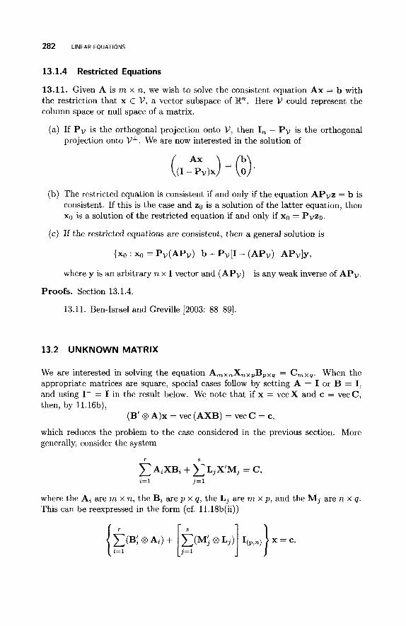
282 LINEAR EQUATIONS
13.1.4 Restricted Equations
13.11. Given A is m x n, we wish to solve the consistent equation Ax = b with the restriction that x E V , a vector subspace of Rn. Here V could represent the column space or null space of a matrix.
(a) If PV is the orthogonal projection onto V , then I, - PV is the orthogonal projection onto V'. We are now interested in the solution of
(b) The restricted equation is consistent if and only if the equation APvz = b is consistent. If this is the case and zo is a solution of the latter equation, then xo is a solution of the restricted equation if and only if xo = PVZO.
(c) If the restricted equations are consistent, then a general solution is
{xO : XO = PV(APV)-b + Pv[I - (APv)-APv]y,
where y is an arbitrary n x 1 vector and (APv)- is any weak inverse of APv.
Proofs. Section 13.1.4.
13.11. Ben-Israel and Greville [2003: 88-89].
13.2 UNKNOWN MATRIX
We are interested in solving the equation AmXnXnXpBpXq = C m x g . When the appropriate matrices are square, special cases follow by setting A = I or B = I, and using I- = I in the result below. We note that if x = vec X and c = vec C, then, by l l . l 6b ) ,
which reduces the problem to the case considered in the previous section. More generally, consider the system
(B' @ A)x = vec (AXB) = vec C = c,
r S
AiXBi + c LjX'Mj = C , i= 1 j = 1
where the Ai are m x n, the Bi are p x q, the Lj are m x p , and the Mj are n x q. This can be reexpressed in the form (cf. 11.18b(ii))
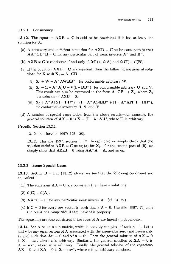
UNKNOWN MATRIX 283
13.2.1 Consistency
13.12. The equation AXB = C is said to be consistent if it has a t least one solution for X.
(a) A necessary and sufficient condition for AXB = C t o be consistent is that AA-CB-B = C for any particular pair of weak inverses A- and B-.
(b) AXB = C is consistent if and only if C(C) c C(A) and C(C’) c C(B’).
(c) If the equation AXB = C is consistent, then the following are general solu- tions for X with XO = A-CB-.
(i) XO + W - A-AWBB- for conformable arbitrary W.
(ii) XO + (I - A-A)U + V(I - BB-) for conformable arbitrary U and V. This result can also be expressed in the form A-CB- + ZO, where ZO is a solution of AZB = 0.
(iii) XO + A-AR(1- BB-) + (I - A-A)SBB- + (I - A-A)T(I - BB-), for conformable arbitrary R, S, and T.
(d) A number of special cases follow from the above results-for example, the general solution of AX = 0 is X = (I - A-A)U, where U is arbitrary.
Proofs. Section 13.2.1.
13.12a-b. Harville [1997: 125-1261,
13.12~. Harville [1997: section 11.121. In each case we simply check that the solution satisfies AXB = C using (a) for XO. For the second part of (ii), we simply show that AZoB = 0 using AA-A = A, and so on.
13.2.2 Some Special Cases
13.13. Setting B = I in (13.12) above, we see that the following conditions are equivalent.
(1) The equations AX = C are consistent (i.e., have a solution).
(3) AA-C = C for any particular weak inverse A- (cf. 13.12a).
(4) k’C = 0 for every row vector k’ such that k’A = 0. Harville [1997: 731 calls the equations compatible if they have this property.
The equations are also consistent if the rows of A are linearly independent.
13.14. Let A be an n x n matrix, which is possibly complex, of rank n - 1. Let u and v be any eigenvectors of A associated with the eigenvalue zero (not necessarily simple) such that Au = 0 and v*A = 0’. Then the general solution of AX = 0 is X = uz’, where z is arbitrary. Similarly, the general solution of XA = 0 is X = wv*, where w is arbitrary. Finally, the general solution of the equations AX = 0 and XA = 0 is X = c u v * , where c is an arbitrary constant.
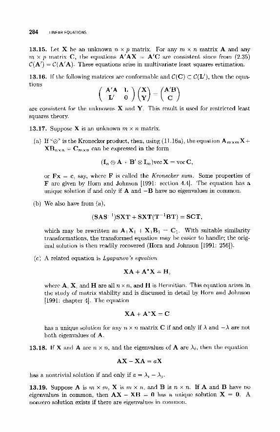
284 LINEAR EQUATIONS
13.15. Let X be an unknown n x p matrix. For any m x n matrix A and any m x p matrix C, the equations A’AX = A’C are consistent since from (2.35) C(A’) = C(A’A). These equations arise in multivariate least squares estimation.
13.16. If the following matrices are conformable and C(C) C C(L’), then the equa- tions
( A;A : ) (Ir) = (A:“)
are consistent for the unknowns X and Y. This result is used for restricted least squares theory.
13.17. Suppose X is an unknown m x n matrix.
(a) If ‘‘8’’ is the Kronecker product, then, using ( l l . l6a) , the equation A,,,X+ XB,,, = C,,, can be expressed in the form
(I, 8 A + B’ 8 1,)vec X = vec C,
or Fx = c , say, where F is called the Kronecker sum. Some properties of F are given by Horn and Johnson [1991: section 4.41. The equation has a unique solution if and only if A and -B have no eigenvalues in common.
(b) We also have from (a),
(SAS-’)SXT + SXT(T-lBT) = SCT,
which may be rewritten as AlXl + XlBl = C1. With suitable similarity transformations, the transformed equation may be easier to handle; the orig- inal solution is then readily recovered (Horn and Johnson [1991: 2561).
(c) A related equation is Lyapunow’s equation
XA + A*X = H,
where A, X, and H are all n x n, and H is Hermitian. This equation arises in the study of matrix stability and is discussed in detail by Horn and Johnson [1991: chapter 41. The equation
X A + A * X = C
has a unique solution for any n x n matrix C if and only if X and -x are not both eigenvalues of A.
13.18. If X and A are n x n, and the eigenvalues of A are Xi , then the equation
AX - XA = aX
has a nontrivial solution if and only if a = X i - X j .
13.19. Suppose A is m x m, X is m x n, and B is n x n. If A and B have no eigenvalues in common, then AX - XB = 0 has a unique solution X = 0. A nonzero solution exists if there are eigenvalues in common.
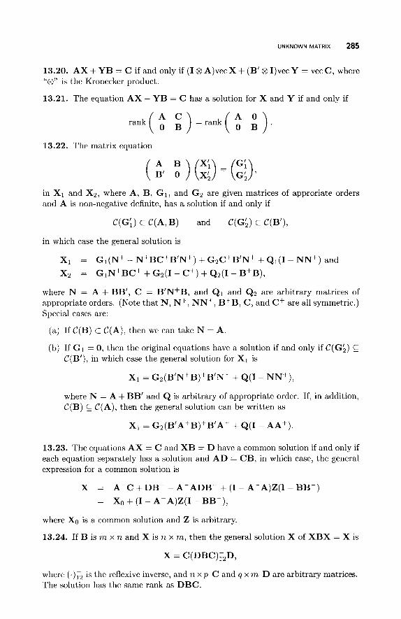
UNKNOWN MATRIX 285
13.20. A X + YB = C if and only if (I @ A)vec X + (B’ @ 1)vecY = vec C, where “8” is the Kronecker product.
13.21. The equation A X - YB = C has a solution for X and Y if and only if
A C A 0 rank ( ) =rank ( ) .
13.22. The matrix equation
A B ( B’ 0 ) (::) = (E:)’ in X1 and X2, where A , B, GI, and G2 are given matrices of approriate orders and A is non-negative definite, has a solution if and only if
C(Gi) c C(A,B) and C(GL) c C(B’),
in which case the general solution is
XI
X2
=
=
G1 (N+ - N+BC+B’N+) + G2C+B’N+ + Q1 (I - N N + ) and
G1N’BC’ + G2(I - C+) + Q2(I - B+B),
where N = A + BB’, C = B’N+B, and Q1 and Qz are arbitrary matrices of appropriate orders. (Note that N, N + , N N t , B+B, C, and C+ are all symmetric.) Special cases are:
(a) If C(B) c C(A), then we can take N = A.
(b) If G1 = 0, then the original equations have a solution if and only if C(G‘,) C C(B’), in which case the general solution for X1 is
Xi = G2(B’N+B)+B‘N+ + Q ( I - N N + ) ,
where N = A + BB’ and Q is arbitrary of appropriate order. If, in addition, C(B) C C(A), then the general solution can be written as
X1 = Gz(B’A+B)+B’A+ + Q(I - A A + )
13.23. The equations A X = C and XB = D have a common solution if and only if each equation separately has a solution and A D = CB, in which case, the general expression for a common solution is
X =
=
A - C + DB- - A-ADB- + (I - A-A)Z(I - BB-)
Xo + (I - A-A)Z(I - BB-),
where Xo is a common solution and Z is arbitrary.
13.24. If B is m x n and X is n x m, then the general solution X of XBX = X is
X = C(DBC),D,
where (.)T2 is the reflexive inverse, and n x p C and q x m D are arbitrary matrices. The solution has the same rank as DBC.
286 LINEAR EQUATIONS
13.25. If B is m x n and X is n x m, then the general solution of XBX = 0 is X = YC, where p as well as the p x m matrix C are arbitrary, and Y is an arbitrary solution of CBY = 0. If X also has to satisfy WBX = 0, then Y is now an arbitrary solution of
(;)BY = 0.
13.26. The equations A l X B l = C1 and A2XB2 = C2 have a common solution if and only if each equation is consistent and
min rank(C1 - AlXB1) = 0, AzXBz=C2
which is equivalent to
0 A1 rank ( ? -C2 A2 ) =rank(A’) + rank(B1, B2).
A proof and further details relating to this problem are given by Tian [2002: 1971
13.27. (Two Unknowns) We wish to consider the solution of the matrix equation AXB + CYD = M for X and Y. Since vec (AXB) = (B’ @ A)vec X, we can rewrite the matrix equation in the form
(B’ @ A, D’ @ C) ( vecY x, = vec M,
which is solvable if and only if (cf. 13.1~)
(B’ @ A, D’ @ C ) (B’ @ A , D’ @ C)-vec M = vec M.
In this case, from (13.4), the general solution is
(:::$) = (B’@A,D’@C)-vecM+ [I - (B’@A,D’@C)-(B’@A,D’@C)]v,
where v is an arbitrary vector. Using his extremal ranks method, Tian [2006b] gives necessary and sufficient rank conditions for solutions X and Y to exist and also provides methods for finding solutions.
Proofs. Section 13.2.2.
13.13. Harville [1997: 731.
13.14. Magnus and Neudecker (1988: 441.
13.16. Harville [1997: 75-76]
13.17a. Graham [1981: 38-39] and Horn and Johnson [1991: 2701.
13.17~. Horn and Johnson [1991: 2701.
13.18. Graham [1981: 401.
13.19. Zhang [1999: 1391 and (b) quoted by Horn and Johnson [1991: 2701.

UNKNOWN MATRIX 287
13.20. Horn and Johnson [1991: 2551.
13.21. Horn and Johnson [1991: 281-2831,
13.22. Magnus and Neudecker [1999: 60-621.
13.23. Ben-Israel and Greville [2003: 541 and Rao and Mitra [1971: 251.
13.24-13.25. Rao and Mitra [1971: 56-57]. They also give solutions to XBXB = XB, BXBX = BX, BXBXB = BXB, and XBXBX = XBX.

This Page Intentionally Left Blank
CHAPTER 14
PARTITIONED MATRICES
Partitioned matrices arise frequently in statistics, especially in proofs. For some partitions and their relationship with ranks, the reader should consult Section 3.6. This chapter is closely linked to the next chapter on patterned matrices.
14.1 SCHUR COMPLEMENT
Definition 14.1. Let E F
A=(. H ) '
where A is possibly rectangular. If E is square and nonsingular, then
S = H - GE-'F = (A/E)
is called the Schur complement of E in A. If H is nonsingular (instead of, or in addition to, E), then
T = E - FH-'G = (A/H)
is the Schur complement of H in A. Schur complements occur in various places in this book, sometimes using a dif-
ferent notation. Because of the wide applicability of Schur complements, we have collected some of the results together here in one place using the present notation, which is the one used in three key references, namely Ouellette [1981], Puntanen
A Matr ix Handbook for Statzsticians. By George A. F. Seber Copyright @ 2008 John Wiley & Sons, Inc.
289
290 PARTITIONED MATRICES
and Styan, [2005b], and Styan [1985]. These writers show how the Schur comple- ment can be used to prove a number of matrix results that are typically proved by other methods. They also show how Schur complements arise naturally in statistics, especially in multivariate analysis and in linear models.
14.1. (Determinants) If A is nonsingular, we have that (see also 14.17)
det E . det(A/E), if E is nonsingular, { det H . det(A/H), if H is nonsingular. det A =
Therefore if A and E are nonsingular, then so is A/E . The same applies to A and H.
14.2. (Ranks) From (3.40a(vi) and (3.4O(vii)) we have:
(a) If E is nonsingular, rankA = rankE + rank(A/E).
(b) If H is nonsingular, rankA = rankH + rank(A/H).
14.3. (Inverses) If A, E, and H are all nonsingular, then:
(a) (A/H)-l = E-l+ E-lF(A/E)- lGE-l .
(b) (A/E)-' = H-l + H- G(A/H) -'FH-~.
14.4. (Inertia) We recall that the inertia Zn(A) of a symmetric matrix A is given by the triple (T+, T - , T O ) , where T+ is the number of positive eigenvalues, T- is the number of negative eigenvalues, and TO is the number of zero eigenvalues. Then, if A is symmetric and E is nonsingular,
Zn(A) = Zn(E) + Zn(A/E).
Ouellette [1981: 207-2101 extends the above result to the case when (A/E) is also part it ioned.
14.5. (Non-negative Definite Matrices) Suppose A is symmetric and E is positive definite.
(a) A is non-negative definite if and only if (A/E) is non-negative definite.
(b) A is positive definite if and only if (
14.6. (Subpartition) Suppose that
/E) is positive definite.
7
K L : F 1
M N : F z . . . . . . . . . . . .
G1 Gz : H
where E and K are nonsingular. Then (E/K) is a nonsingular leading principal submatrix of (A/K), and
(WE) = ( (A/K)/(E/K)) .
SCHUR COMPLEMENT 291
14.7. (Sum) Let
be symmetric (m + n) x (m + n) matrices, where E and K are m x m. Suppose that A and B are non-negative definite (n.n.d.) and E and K are positive definite.
F’E-’F + L’K-lL - (F + L)’(E + K)-’(F + L) is n.n.d. with the same rank as F - EK-lL.
( (A + B)/(E + K)) - (A/E) - (B/K) is n.n.d.
Definition 14.2. (Generalized Schur Complement) Referring to Definition 14.1, if E is rectangular, or square and singular, then we replace E-’ by any weak inverse E- and call (A/E) the generalized Schur complement of E in A . We have a similar definition for (A/H).
We shall use the following notation below:
S = (A/E) = H - GE-F and T = (A/H) = E = FH-G.
14.8. (General Properties of the Generalized Schur Complement)
(a) If A and E are both square and either C(F) C C(E) or C(G’) C(E’), then S is invariant for all weak inverses E- and
det A = det E . det S.
(b) If A and H are both square and either C(G) C C(H) or C(F’) C(H’), then T is invariant for all weak inverses H- and
det A = det H . det T.
(c) If A is non-negative definite and E and H are both square (i.e., G = F‘), then C(F) C C(E) and C(F’) C(H); also (a) and (b) hold.
14.9. Suppose A is non-negative definite and E and H are both square, then:
(a) S and T are invariant with respect to the weak inverses E- and H-
(b) (Rank)
(i) rank A = rank E + rank(A/E) . (ii) rank A = rank H + rank(A/H).
(c) (Inertia)
(i) Zn(A) = Zn(E) + Zn(A/E).
(ii) Zn(A) = Zn(H) + Zn(A/H).
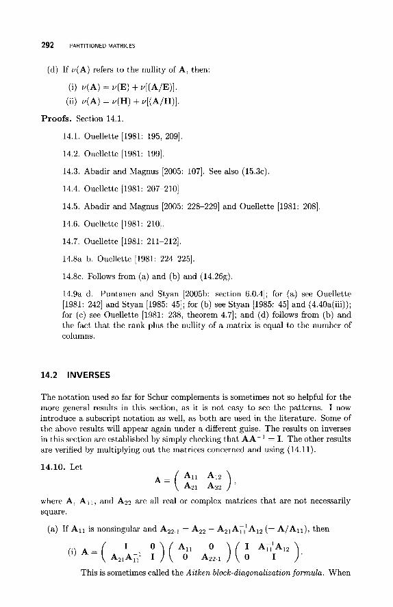
292 PARTITIONED MATRICES
(d) If v(A) refers to the nullity of A, then:
(i) v(A) = v(E) + v[(A/E)].
(ii) v(A) = v(H) + v[(A/H)].
Proofs. Section 14.1.
14.1. Ouellette [1981: 195, 2091.
14.2. Ouellette [1981: 1991.
14.3. Abadir and Magnus [2005: 1071. See also (15.3~).
14.4. Ouellette [1981: 207-2101
14.5. Abadir and Magnus [2005: 228-2291 and Ouellette [1981: 2081.
14.6. Ouellette [1981: 2101.
14.7. Ouellette [1981: 211-2121.
14.8a-b. Ouellette [1981: 224-2251,
14.8~. Follows from (a) and (b) and (14.26g).
14.9a-d. Puntanen and Styan [2005b: section 6.0.41; for (a) see Ouellette [1981: 2421 and Styan [1985: 451; for (b) see Styan [1985: 451 and (4.40a(iii)); for (c) see Ouellette [1981: 238, theorem 4.71; and (d) follows from (b) and the fact that the rank plus the nullity of a matrix is equal t o the number of columns.
14.2 INVERSES
The notation used so far for Schur complements is sometimes not so helpful for the more general results in this section, as it is not easy to see the patterns. I now introduce a subscript notation as well, as both are used in the literature. Some of the above results will appear again under a different guise. The results on inverses in this section are established by simply checking that AA-' = I. The other results are verified by multiplying out the matrices concerned and using (14.11).
14.10. Let
A = ( 2;; ) , where A, All , and A22 are all real or complex matrices that are not necessarily square.
(a) If All is nonsingular and A,,., = A,, - A,,AT~A,, (= A/A11), then
This is sometimes called the Aitken block-diagonalization formula. When
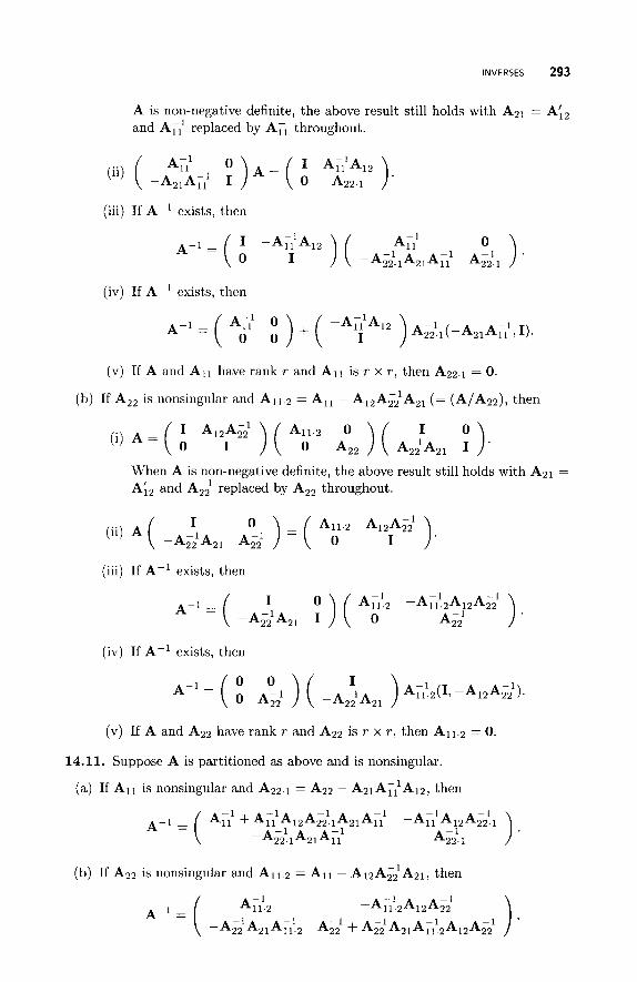
INVERSES 293
A is non-negative definite, the above result still holds with Azl = A{2 and A,' replaced by ATl throughout.
(iii) If A-' exists, then
(iv) If A p l exists, then
(v) If A and All have rank r and Al l is r x r, then A22.1 = 0.
(b) If A,, is nonsingular and All.2 = A,, - A12Ag;A21 (= (A/A22), then
(i) A = ( ; .,2;;; ) ( All.2 o 12) ( A;{A21 ;). When A is non-negative definite, the above result still holds with A21 =
Ai2 and A;. replaced by Ai2 throughout.
(iii) If A-' exists, then
(iv) If A-' exists, then
(v) If A and A22 have rank r and A22 is r x r, then All.2 = 0.
14.11. Suppose A is partitioned as above and is nonsingular.
(a) If A l l is nonsingular and A22.1 = A22 - A21ATIlA12, then
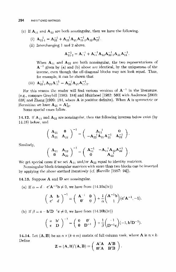
294 PARTITIONED MATRICES
(c) If A,, and A,, are both nonsingular, then we have the following.
(i) A;;l = A;. + A;;A21AT:2A12A2;]
(ii) Interchanging 1 and 2 above,
AT:., = AT: + A ~ ~ A 1 2 A ; ~ l A 2 1 A ~ ~
When All and A22 are both nonsingular, the two representations of A-l given by (a) and (b) above are identical, by the uniqueness of the inverse, even though the off-diagonal blocks may not look equal. Thus, for example, it can be shown that
(iii) A,- , f ,A , ,A~~ = A;;A21AT:2.
For this reason the reader will find various versions of A-' in the literature. (e.g., compare Graybill [1983: 1841 and Muirhead [1982: 5801 with Anderson [2003: 6381 and Zhang [1999: 184, where A is positive definite). When A is symmetric or Hermitian we have A21 = AT,.
Some special cases follow.
14.12. If A,, and A,, are nonsingular, then the following inverses below exist (by 14.18) below, and
Similarly,
A,, ) - I = ( AT; -AT;A12&. ) ( Ad' A,, 0 A;;
We get special cases if we set All and/or A22 equal to identity matrices.
by applying the above method iteratively (cf. Harville [1997: 941).
14.13. Suppose A and D are nonsingular.
Nonsingular block-triangular matrices with more than two blocks can be inverted
(a) If a = d - c'A-'b # 0, we have from (14.10a(iv))
A b A-l 0 (c'A-1,-1) ( c ' d ) - l = ( 0' o)+n( - 1 )
(b) If p = a - b'D-'c # 0, we have from (14.10b(iv))
14.14. Let (A, B) be an n x ( k + rn) matrix of full column rank, where A is n x k . Define
Z = (A, B)'(A, B) = ( ;;; ;;; )
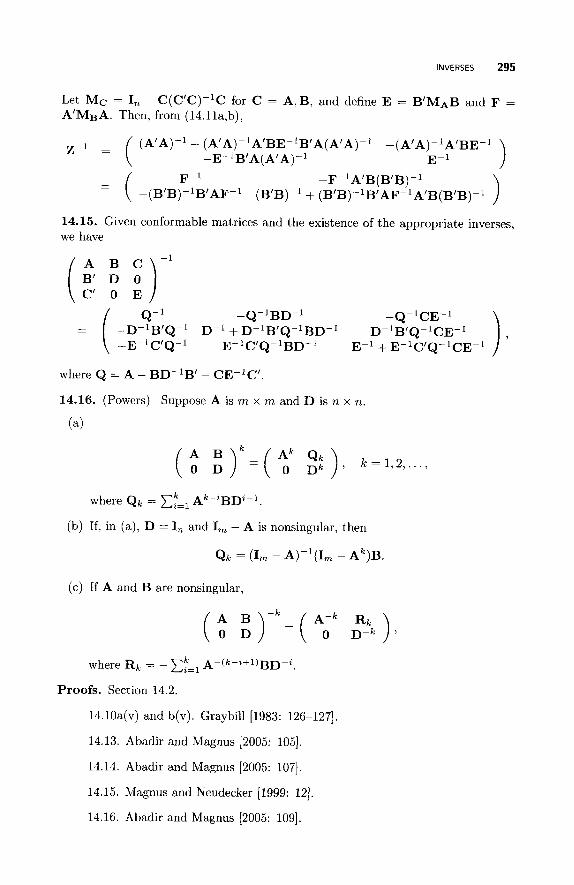
INVERSES 295
Let M c = I, - C(C’C)-’C for C = A , B , and define E = B’MAB and F = A‘MBA. Then, from (14.11a,b),
14.15. Given conformable matrices and the existence of the appropriate inverses, we have
where Q = A - BD-lB’ - CE-IC’
14.16. (Powers) Suppose A is m x m and D is n x n.
(4
( t :)*=( tk ::), k = 1 , 2 , . . . ,
where Q k = C,“=, A”ZBDz-’.
(b) If, in (a), D = I, and I, - A is nonsingular, then
Qk = (I, - A)-’& - A”B.
(c) If A and B are nonsingular,
14.10a(v) and b(v). Graybill [1983: 126-1271.
14.13. Abadir and Magnus 12005: 1051.
14.14. Abadir and Magnus [2005: 1071.
14.15. Magnus and Neudecker (1999: 121.
14.16. Abadir and Magnus [2005: 1091
296 PARTITIONED MATRICES
14.3 DETERMINANTS
14.17. Suppose A is partitioned as in (14.10).
(a) If A,, is nonsingular,
det A = det(A,,) det(A22.1).
If, in addition, A is nonsingular, then so is A22.1, the Schur complement of
Al l .
(b) If A,, is nonsingular,
det A = det(A,,) det(All.2).
If, in addition, A is nonsingular, then so is All.,, the Schur complement of
A,,.
(c) If A, and A;, are any weak inverses of Al l and A22, then:
(i) If C(A21) s C(A22) or C(Ai,) C(Ah,), we have
det A = (det A22) det(A11 - A12Ai2A21).
(ii) If C(A12) C C(A11) or C(Ah,) C(A;,), we have
det A = (det Al l ) det(A22 - A21A;lA12).
14.18. The following two results are often useful.
(a) If A and B are m x m and n x n, respectively, then, for conformable matrices,
d e t ( A 0 ) = d e t ( ) = d e t A . d e t B .
We can set A or B equal to the identity matrix.
Note that the two matrices on the left are nonsingular if and only if both A and B are nonsingular.
(b) Using a similar notation to (a),
O F B E d e t ( .) = d e t ( ) = ( - l ) m n d e t E . d e t F .
14.19. If B and C are n x n matrices, then
det ( -in ) = detB.
14.20. If C = (A,B) is square, then from det(CC’) = det(C’C) = det(C), we have
det(AA’ + BB’) = det B’A B’B ( A‘A A’B )
DETERMINANTS 297
14.21. Let A and D be square matrices. Then:
(a) det ( ) = ddet A - c’(adjA)b,
or det A(d - c’A-lb) if A is nonsingular, where adjA is the adjoint matrix of A.
(b) det ( ) = det D(a - b’D-’c) if D is nonsingular.
det ( A + uu’).
be an n x n matrix such that E is m x m. If
adjA = ( g: i: ) , where El is m x m, then:
(a) det HI = (det
(b) det El = (det A)” det H, for m = 0,1,2, . . . , n - 1.
d e t E form = 0 ,1 ,2 , . . . , n - 1
14.23. If A C = CA. then
det ( ) = det(AD - CB).
If we set A = I, then the above is true.
14.24. If A and B are n x n matrices, then
det ( ) = d e t ( A + B ) . d e t ( A - B ) .
14.25. The determinant of the matrix inversed in (14.15) is
det D . det E . det(A - BD-lB’ - CE-lC’).
Proofs. Section 14.3.
14.17a. We take determinants in (14.10a(i)) and use the fact that the deter- minant of a triangular matrix is the product of its diagonal elements.
14.17b. Similar to (a), but using (14.10b(i)).
14.17~. Schott [2005: 2631; see also (14.8a,b).
14.18a. Harville [1997: 1851, Rao and Bhimasankaram [2000: 2341, and Searle [1982: 971.
298 PARTITIONED MATRICES
14.18b. Harville [1987: 1871
14.19. This follows from (14.18b) and the fact that n2 + n = n(n + 1) is even. See also Searle [1982: 981.
14.21. Abadir and Magnus [2005: 1131
14.22. Ouellette [1981: 205-2061.
14.23. Abadir and Magnus [2005: 1161
14.24. Abadir and Magnus [2005: 1171
14.25. Abadir and Magnus [2005: 1181
14.4 POSITIVE AND NON-NEGATIVE DEFINITE MATRICES
Schur complements arise in this section using a different notation, and the results should be compared with those in Section 14.1. Note that A >. B means that A-B is non-negative definite.
14.26. Let
be a real symmetric matrix (i.e., A12 = A;,, with All and A22 square matrices).
if and only if All and A22 - (a) A + 0 (i.e., is positive definite or p.d.)
(b) A + 0 if and only if A22 and All - A12A;iA21 are p.d.
(c) If A + 0, then
A21AT:A12 (= (A/A11) are p.d.
A22 ? A22 - A2iAT:Ai2.
(d) If A + 0 and A’’ is the leading principal submatrix of A-’ with the same size as A1 1 , then
A” - AT: 2 0.
(e) (Fischer Inequality) If A + 0, then
det A L det All . det A22,
with equality if and only if both sides vanish or A12 = 0.
(f) If A 2 0 and the blocks All, A12, and A22 are square matrices of the same size, then
I det A12I2 5 det All det A22.
(g) If A k 0, then C(A12) C C(A11) and C(A21) C C(A22).
The above results will also hold if A is Hermitian.
POSITIVE AND NON-NEGATIVE DEFINITE MATRICES 299
14.27. Let the real symmetric matrix A be partitioned as in (14.10) above, where All + 0. Then for any square matrix A22 k 0,
A 5 0 if and only if A22 k AZIA;;A~Z.
14.28. Let
where All is a non-negative definite m x m matrix and A12 is m x n. The symmetric (m + n) x (m + n) matrix A is sometimes referred to as a borderd Gramian matrix.
(a) A is nonsingular if and only if rankAl2 = n and All + A12Ai2 is positive definite.
(b) If A is nonsingular, and setting A21 = Ai2, then
where B11 = All + A12AZ1 and B22 = A21BT:A12.
(c) If B11 above is nonsingular, then
de tA = (-l),detB11 'detB22.
(d) If A is nonsingular, then
det A = (-l), det All . det(A21AT;Alz).
14.29. Let A be positive definite and let B = ( real.
), where A, b, and c are
(a) det B = det A(c - b'A-lb) 5 cdet A, with equality if and only if b = 0.
(b) B is positive definite if and only if det B > 0.
(c) If c = b'A-lb, then B is non-negative definite.
(d) x'Ax - 2b'x 2 -b'A-'b.
14.30. Let A and B be real n x n matrices, and let
where A1 and B1 are positive definite. Then
a:A;lal + biBF'b1 - (a1 + bl)'(Al + Bl)-'(al + bl) = (ATlal - BT1bl)'(All + B[')-'(AF1al - B,'bl).
Anderson [2003: 4191 gives an application to testing that several multivariate nor- mal populations are identical.
300 PARTITIONED MATRICES
14.31. Let A and B be n x n positive definite matrices. There exists a unique matrix C such that
Cy = azj, ( i , j ) E { 1 , 2 . . . . , t } cZJ = b'J, ( i , j ) $ { 1 , 2 , . . . , t }
where C-' = c23 and B-' = bzJ . This result has an application to graphical models for determining patterns of independence.
Proofs. Section 14.4.
14.26a. Horn and Johnson [1985: 472, complex case] and Zhang [1999: 175, complex case].
14.26b. Same as (a) with the subscripts 1 and 2 interchanged.
14.26~. Horn and Johnson [1985: 474, in proof of theorem 7.7.81 and Zhang [1999: 175, complex case].
14.26d. Follows from (14.11a); see also Zhang [1999: 175, complex case].
14.26e. Horn and Johnson [1985: 4781 and Zhang [1999: 175, complex case].
14.26f. Abadir and Magnus [2005: 228, 3411.
14.26g. Sengupta and Jammalamadaka [2003: 451; see also (14.8~).
14.27. Zhang [1999: 178, complex case].
14.28. Abadir and Magnus [2005: 230-2311,
14.29. Magnus and Neudecker [1988: 23-24].
14.30. Anderson [2003: 4191.
14.31. Anderson [2003: 614, 6161.
14.5 EIGENVALUES
In this section we assume that the n x n matrix A is partitioned as in (14.10) with Aii being ni x ni, for i = 1,2 (nl + 722 = n). We also continue with the notation XI(A) 2 . . . 2 X,(A) for ordering the eigenvalues when they are real, which is the case for a symmetric matrix.
14.32. Suppose A is non-negative definite. If h and i are integers between 1 and n inclusive, then:
(a) Xh+i-l(A) I h(A11) + Xi(&) , if h + I n + 1,
(b) h + i ~ ~ ( A ) 2 Xh(A11) + Xi(A22), if h + i 2 n + 1,
where Xh(A11) = 0 if h > n1 and Xi(A22) = 0 if i > 722.
EIGENVALUES 301
14.33. Suppose A is non-negative definite and i l , i 2 , . . . , ak are distinct integers beween 1 and n, inclusive. Then for k = 1 ,2 , . . . , n,
k k
CIXtl (Ail) + & - ~ + ~ ( A z z ) ] 5 C Atl (A) j=1 3=1
k
I C[Xt3(All) + X ~ ( A ~ Z ) ] , 3=1
where Xj(Al1) = 0 if j > n1 and Xj(A22) = 0 if j > nz
14.34. Suppose A is symmetric and Xnl(A1l) > Xl(A22).
(a) For j = 1,2, . . . ,711,
and for j = 1 ,2 , . . . , nz,
Tighter bounds are given by Dumbgen [1995]. The above bounds are use- ful in obtaining the asymptotic distribution of the eigenvalues of a random symmetric matrix (Eaton and Tyler [1991]).
(b) For k = 1 ,2 , . . . ,121,
14.35. Suppose A is positive definite, and let B1 = A11 - A12A,-,'A21, Bz = Az2 - AZ1A;;Al2, and C = -B;lAlzA,-,', where A12 = ALl. Then if Xl(B1) < Xnz(B2),
for k = l , 2 , . . . , n1.
Proofs. Section 14.5.
14.32-14.34. Schott [2005: 271-2731.
14.35. Schott [2005: 275-2761,
302 PARTITIONED MATRICES
14.6 GENERALIZED INVERSES
14.6.1 Weak Inverses
14.36. Let A = (All,A12), where All is nonsingular. Then
is a weak inverse of A for arbitrary Y.
14.37. Let A = (ti:), where All is nonsingular. Then
A- = (A:; - XA,,A,-,', X)
is a weak inverse of A for arbitrary X
14.38. Let A be m x n.
(a) (;I) is a weak inverse of (A, B) if and only if AA-B = 0 and BB-A = 0.
(b) (Ap, C-) is a weak inverse of (t) if and only if CA-A = 0 and AC-C = 0.
For conditions on the ranks for the above weak inverses to hold, see Tian [2005b].
14.39. Let A1(pxn) and G = (Gl(nx,), G2(nxq)),
A = (A2(qxn))
with p + q = m. Then C(A{) nC(Ah) = 0 and G is a weak inverse of A if and only if
AIGIAl = Al , A2G1Al= 0, A2G2A2 = A2, and AlGzA2 = 0.
If rank A1 = p, the first two equations above become AlGl = I, and A2G1 = 0.
14.40. Let
with p + q = n. Then C(A1) n C(A2) = 0 and G is a weak inverse of A if and only if
AIGIAl = Al, AlGlAz = 0, A2G2A2 = A2, and A2G2A1= 0.
If rank Al = p , the first two equations above become GlAl = I, and G1A2 = 0.
14.41. Let A be partitioned in the form of (14.10).
C(A11), C(Ahl) (a) If C(A12) C(A{,), ATl is a particular weak inverse of All , and A,,., = A,, - A2,AF1Al2, we have
A22.1
GENERALIZED INVERSES 303
(b) If C(A21) C C(A22), C(Ai2) C C(AL2), A, is a particular weak inverse of A22, and A,,., = A,, - A,2A~2A2,, we have
All.2 -A,.,A12A22
-A22A21A,.2 A22 i- A22A21Al1.2A12A22 A- = (
Necessary and sufficient conditions are given in (14.44) below using a different notation. Some rank conditions for the above to hold are given by Tian and Takane [2005].
14.42. Let A be an n x n non-negative definite matrix partitioned as in (14.10), where All is p x p . Suppose that the n x n matrix G is a weak inverse of A and is partitioned in exactly the same way as A. If each of the first p rows of A is nonzero and is not a linear combination of the remaining rows of A, then
Gii = (Ail - Ai2A&21)-~
for any weak inverse Ai2 of A22. Also G11 is unique.
where V is an n x n non-negative definite matrix, X is n x p, and G11 is n x n.
(a) If G is a weak inverse of A, we have the following.
(i) GI2 is weak inverse of of X’.
(ii) G2l is weak inverse of of X.
(iii) VG12X’ = XG2lV = -XG22X’.
(iv) VGllX = 0, X’G11V = 0, and X’G11X = 0.
(v) V = VGllV - XG22X’.
(vi) VGllV, VG12X’, XG2,V1 and XG22X‘ are symmetric and invariant to the choice of the weak inverse G.
(b) If U is any p x p matrix such that C(X) C(V + XUX’), and W is any weak inverse of V + XUX’, then
w - WX(X‘WX)-X‘W wx(x‘wx)- ( (X‘WX) ~ X’W -(X’WX)- + u is a weak inverse of A.
14.44. Let E F
. = ( G H ) ’
(a) Let E be a particular weak inverse of E and S = H - GEF, the generalized Schur complement. Then
E + EFS-GE -EFS- B = ( -S-GE S -
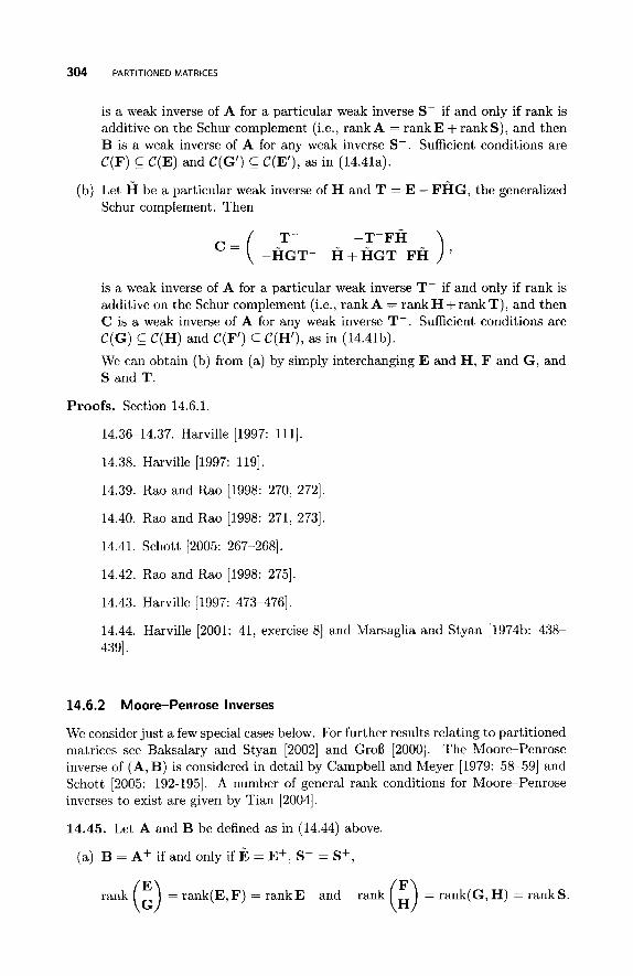
304 PARTITIONED MATRICES
is a weak inverse of A for a particular weak inverse S- if and only if rank is additive on the Schur complement (i.e., rankA = r ankE+rankS) , and then B is a weak inverse of A for any weak inverse S - . Sufficient conditions are C(F) s C(E) and C(G’) C C(E’), as in (14.41a).
(b) Let H be a particular weak inverse of H and T = E - FHG, the generalized Schur complement. Then
1 T- -T-FH -HGT- H + HGT-FH ’ c = (
is a weak inverse of A for a particular weak inverse T- if and only if rank is additive on the Schur complement (i.e., rankA = r ankH+rankT) , and then C is a weak inverse of A for any weak inverse T- . Sufficient conditions are
C(G) We can obtain (b) from (a) by simply interchanging E and H, F and G , and S and T .
C(H) and C(F’) C C(H’), as in (14.41b).
Proofs. Section 14.6.1
14.36-14.37. Harville [1997: 1111
14.38. Harville [1997: 1191.
14.39. Rao and Rao [1998: 270, 2721
14.40. Rao and Rao [1998: 271, 2731
14.41. Schott [2005: 267-2681,
14.42. Rao and Rao [1998: 2751.
14.43. Harville [1997: 473-4761.
14.44. Harville [2001: 41, exercise 81 and Marsaglia and Styan [1974b: 438- 4391.
14.6.2 Moore-Penrose Inverses
We consider just a few special cases below. For further results relating to partitioned matrices see Baksalary and Styan [2002] and Groa [2000]. The Moore-Penrose inverse of (A, B) is considered in detail by Campbell and Meyer [1979: 58-59] and Schott [2005: 192-1951, A number of general rank conditions for Moore-Penrose inverses to exist are given by Tian [2004].
14.45. Let A and B be defined as in (14.44) above.
(a) B = A+ if and only if E = E+, S- = S+,
rank (E) = rank(E,F) = rankE and rank (E) = rank(G,H) = r a n k s .
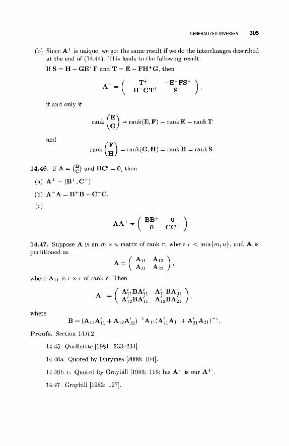
GENERALIZED INVERSES 305
(b) Since A+ is unique, we get the same result if we do the interchanges described at the end of (14.44). This leads to the following result.
If S = H - GE+F and T = E - FH+G, then
T+
if and only if
rank (:) = rank(E, F) = rank E = rank T
and
rank (E) = rank(G, H) = rank H = rank S.
14.46. If A = (g) and BC' = 0, then
(a) A+ = (B+,C+)
(b) A+A = BfB + C+C.
(c)
A A + = ( Br+ ci+ ) 14.47. Suppose A is an m x n matrx of rank r , where r < min{m,n}, and A is partitioned as
A = ( 2:; A22 ) ' where All is r x r of rank r . Then
where B = (AHA:, + A12A:2)-1A11(A;,A11 + A;lA21)-'
Proofs. Section 14.6.2.
14.45. Oiiellettte [1981: 233-2341,
14.46a. Quoted by Dhrymes [2000: 1041.
14.46b-c. Quoted by Graybill [1983: 115; his A- is our A+]
14.47. Graybill [1983: 1271.
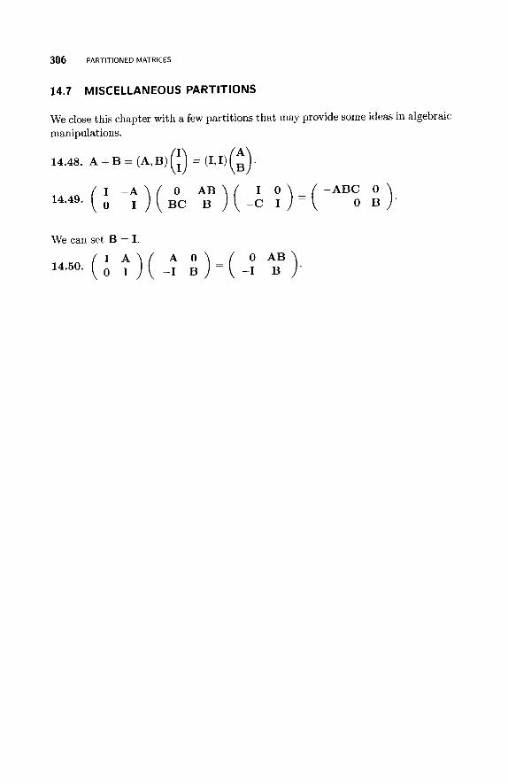
306 PARTITIONED MATRICES
14.7 M I SC EL LAN EO U S PA RTlT I0 N S
We close this chapter with a few partitions that may provide some ideas in algebraic manipulations.
0 A " ) ( I O ) = ( -ABC 0 ) 14.49' ( -; ) ( BC B -c I O B '
We can set B = I.
A 0 0 AB 14*50' ( ) ( -I B ) = ( -I B ) '
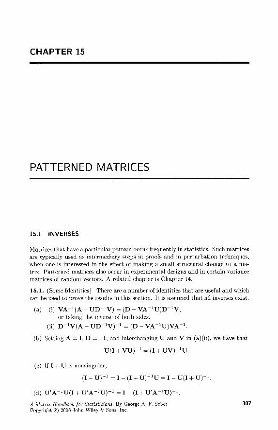
CHAPTER 15
PATTERNED MATRICES
15.1 INVERSES
Matrices that have a particular pattern occur frequently in statistics. Such matrices are typically used as intermediary steps in proofs and in perturbation techniques, when one is interested in the effect of making a small structural change to a ma- trix. Patterned matrices also occur in experimental designs and in certain variance matrices of random vectors. A related chapter is Chapter 14.
15.1. (Some Identities) There are a number of identities that are useful and which can be used to prove the results in this section. It is assumed that all inverses exist.
(a) (i) VA-'(A - UD-'V) = (D - VA-'U)D-'V,
(ii) D-'V(A - UD-lV)-' = (D - VA-'U)VA-'.
or taking the inverse of both sides,
(b) Setting A = I, D = -I, and interchanging U and V in (a)(ii), we have that
U(I + vu)-' = (I + uv)-lu.
(c) If I + U is nonsingular,
(I + u)-1 = I - (I + U ) - w = I - U(I + u)-'.
(d) U'A-'U(I + U'A-'U)-' = I - (I + U'A-lU)-'.
A Matrix Handbook for Statisticians. By George A. F. Seber Copyright @ 2008 John Wiley & Sons, Inc.
307
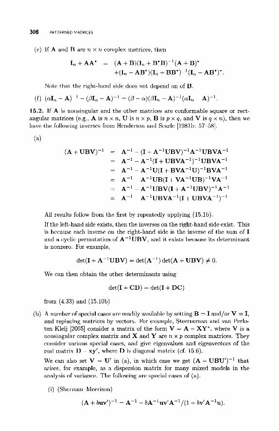
308 PATTERNED MATRICES
(e) If A and B are n x n complex matrices, then
1, + AA' = (A + B)(I, + B*B)-'(A + B)*
+(In. - AB*)(I, +BB*)-l(1, -AB*)*.
Note that the right-hand side does not depend on of B.
15.2. If A is nonsingular and the other matrices are conformable square or rect- angular matrices (e.g., A is n x n, U is n x p , B is p x q, and V is q x n) , then we have the following inverses from Henderson and Searle (1981b: 57-58].
(A + UBV)-' = A-' - (I + A-'UBV)-'A-'UBVA-'
A-' - A-'(I + UBVA-')-'UBVA-'
A-' - A-'U(1 + BVA-'U)-'BVA-'
A-' - A-'UB(1 + VA-'UB)-'VA-'
A-l - A-'UBV(1 + A-'UBV)-'A-'
A-' - A-'UBVA-'(I + UBVA-')-'
=
=
=
=
=
All results follow from the first by repeatedly applying (15.1b).
If the left-hand side exists, then the inverses on the right-hand side exist. This is because each inverse on the right-hand side is the inverse of the sum of I and a cyclic permutation of A-lUBV, and it exists because its determinant is nonzero. For example,
det(I+ A-'UBV) = det(A-') det(A + UBV) # 0.
We can then obtain the other determinants using
de t ( I+ CD) = det ( I+ DC)
from (4.33) and (15.10b)
(b) A number of special cases are readily available by setting B = I and/or V = I, and replacing matrices by vectors. For example, Steerneman and van Perlo- ten Kleij [2005] consider a matrix of the form V = A - XY*, where V is a nonsingular complex matrix and X and Y are n x p complex matrices. They consider various special cases, and give eigenvalues and eigenvectors of the real matrix D - xy', where D is diagonal matrix (cf. 15.6).
We can also set V = U' in (a), in which case we get (A + UBU')-' that arises, for example, as a dispersion matrix for many mixed models in the analysis of variance. The following are special cases of (a).
(i) (Sherman-Morrison)
(A + buv')-' = A-' - bA-'uv'A-'/(l+ bv'A-'u).
INVERSES 309
This is used as an "updating" formula discussed further in (15.11). The situation when A or the modified matrix is singular is investigated by Baksalary and Baksalary [2004c] (see also Section 15.5.2).
x'A-'x 1 + x 'A-~x '
(ii) x'(A + xx')-'x =
(iii) (A + UBU')-' = A-' - A-'UB(I + U'A-'UB)-lU'A-l.
For a good historical discussion and further results see Henderson and Searle [1981b]. They also give some statistical applications of these identities such as inverting the variance matrix for a multinomial vector, inverting a matrix with the pattern of an intraclass correlation matrix, and obtaining the generalized least squares estimates for a variance component model.
15.3. Another set of results can be derived by assuming that B is also nonsingular. From the fourth equation of (15.2a) we have:
(a) (i) (A + UBV)-' = A-' - A-'UB(B + BVA-'UB)-'BVA-'.
(ii) (A + UBV)-' = A-' - A - 'U(B-' + VA-lU)-lVA-l.
(iii) Setting B = I, we have the sc-called Sherman-Morrison- Woodbvry for- mula
(A + UV)-' = A-' - A-'U(I + VA-lU)-'VA-'
This result also holds with A Hermitian.
(iv) Setting A and B equal to identity matrices in ( i ) or (ii), we have
(I + uv)-' = I - U(I + vu)-'v
(b) Setting V = U' in (a)(ii) gives us
(i) (A + UBU')-' = A-' - A-lU(B-' + U'A-'U)-'U'A-'.
(ii) If C = (U'A-'U)-' exists, then using (15.4b) with B and C instead of A and B, we have
(iii) In particular,
We can also interchange A and B and can replace A by A-' and B by B-1.
We note that in (b) (and (a)) we can replace B by -B.
310 PATTERNED MATRICES
(c) Setting B = -D-' in (a)(ii) leads to a number of results like the following:
(i) (A - UD-'V)-' = A-l + A - 'U(D - VA-lU)-lVA-l.
Note that the left-hand side of the above is the inverse of a Schur com- plement. As a special case we have
(ii) (I - UV)-l = I + U(I - VU)-lV, as in (a)(iv) with a sign change.
15.4. Gentle [1998: 621 notes that in linear regression we often need inverses of various sums of matrices and gives the following additional identities for nonsingular A and B.
(a) (A + BB')-lB = A-'B(I + B'A-'B)-l.
(b) (Ap1 + B-l)-l = A(A + B)-'B.
(c) A(A + B)-'B = B(A + B)-lA.
(d) Apl + B-' = A-l(A + B)B-'
We can also add, for nonsingular A + B,
( e ) A - A(A + B)-lA = B - B(A + B)-'B.
15.5. (Non-negative Definite Matrices)
(a) If A is positive definite, then A - bb' is positive definite if and only if b'A-lb < 1.
(b) If A is non-negative definite (n.n.d.), then A - bb' is n.n.d. if and only if b E C(A) and b'A-b 5 1.
15.6. If A = diag(a1, a2, . . . ,a,) is a nonsingular diagonal matrix and C = A + cyuv', then we have the following.
(a) C-' = A-l + ap-lfg', where ,b' = -(1 + ~ C ~ = ~ ( u i w i / a i ) (# 0) , f i = ui /a i , and gi = wi/ai.
(c) The characteristic equation of C is given by
For further details relating to the eigenvalues and eigenvectors of C see Steerneman and van Perlo-ten Kleij [2005] and the references therein.
(d) If a1 = a2 = . . . = a, = a, then C has n - 1 eigenvalues equal to a and one eigenvalue equal to a + cy CrE1 uivi.
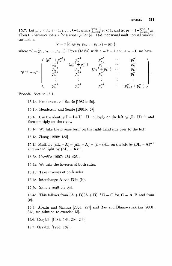
INVERSES 311
15.7. L e t p i > O f o r i = 1 , 2 , . . . , k - l , w h e r e C ~ ~ ~ p p i < l , a n d l e t p k = l - C , = l p ~ . k-1
Then the variance matrix for a nonsingular ( k - 1)-dimensional multinomial random variable is
V = n{diag(pl,pz,. . . , Pk-1) - PP'},
where p' = (pl, pz, . . . , pk-1). From (15.6a) with n = k - 1 and Q = - 1, we have
-1
-1
-1
-1
pk pk
(pT1 + p i 1 ) . . . pk pk
. . . -1 -1
-1 pk
. . . -' (Pz' +Pi1) Pk -1
-1
-1
-1
pk pk pk
pk pk pk . . . -1
. . . (PL21 +P i1 ) -1 -1 -1
pk pk pk
v-1 = n-l
Proofs. Section 15.1.
15.la. Henderson and Searle [1981b: 561.
15.lb. Henderson and Searle [1981b: 571.
15.1~. Use the identity I = I + U - U, multiply on the left by (I + U)-', and then multiply on the right.
15.ld. We take the inverse term on the right-hand side over to the left.
15.le. Zhang [1999: 1851.
15.lf. Multiply (PI, - A) - (@I, -A) = ( p - a)In on the left by (PIn - A)-' and on the right by (@I, - A)-'.
15.3a. Harville [1997: 424-4251.
15.4a. We take the inverses of both sides.
15.4b. Take inverses of both sides.
15 .4~ . Interchange A and B in (b).
15.4d. Simply multiply out.
15.4e. This follows from (A + B)(A + B)-lC = C for C = A, B and from
( c ) .
15.5. Abadir and Magnus [2005: 2271 and Rao and Bhimasankaram [2000: 345, see solution to exercise 151.
15.6. Graybill [1983: 189, 203, 2061.
15.7. Graybill [1983: 1891.
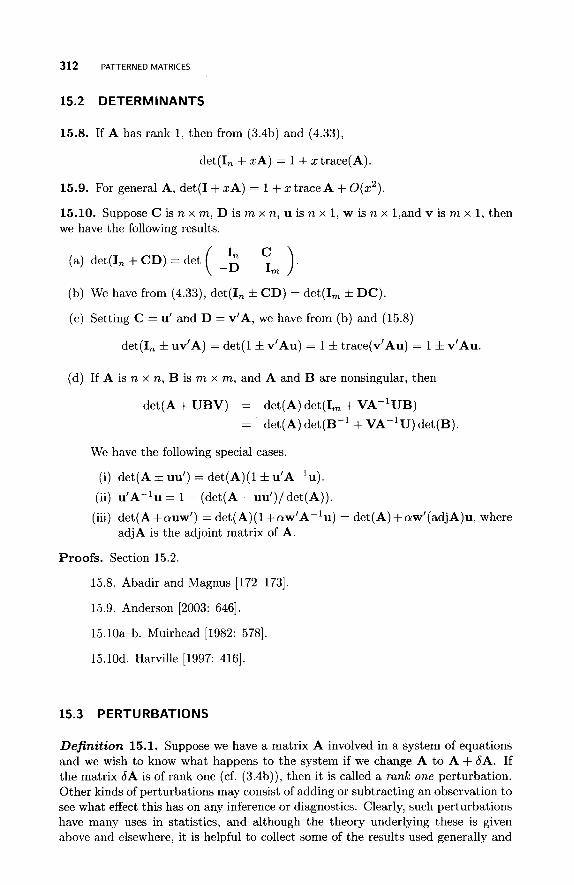
312 PATTERNED MATRICES
15.2 DETERMINANTS
15.8. If A has rank 1, then from (3.4b) and (4.33),
det(1, + zA) = 1 + ztrace(A).
15.9. For general A, det(1 + zA) = 1 + z traceA + O(z2).
15.10. Suppose C is n x m, D is m x n, u is n x 1, w is n x 1,and v is m x 1, then we have the following results.
(a) det(1, + CD) = det (2 ;,) (b) We have from (4.33), det(1, f CD) = det(1, f DC).
(c) Setting C = u’ and D = v’A, we have from (b) and (15.8)
det(1, f uv’A) = det(1 f v’Au) = 1 f trace(v’Au) = 1 f v’Au.
(d) If A is n x n, B is m x m, and A and B are nonsingular, then
det(A + UBV) = det(A) det(1, + VA-’UB) = det(A) det(B-’ + VA-lU) det(B).
We have the following special cases.
(i) det(A * uu‘) = det(A)(l f u’A-lu).
(ii) u ‘ A - ~ u = 1 - (det(A - uu’)/det(A)).
(iii) det(A+auw’) = det(A)(l+aw’A-’u) = det(A)+aw’(adjA)u, where adjA is the adjoint matrix of A.
Proofs. Section 15.2.
15.8. Abadir and Magnus [172-1731.
15.9. Anderson [2003: 6461.
15.10a-b. Muirhead [1982: 5781.
15.10d. Harville [1997: 4161.
15.3 PERTURBATIONS
Definition 15.1. Suppose we have a matrix A involved in a system of equations and we wish to know what happens to the system if we change A to A + &A. If the matrix bA is of rank one (cf. (3.4b)), then it is called a rank one perturbation. Other kinds of perturbations may consist of adding or subtracting an observation to see what effect this has on any inference or diagnostics. Clearly, such perturbations have many uses in statistics, and although the theory underlying these is given above and elsewhere, it is helpful to collect some of the results used generally and
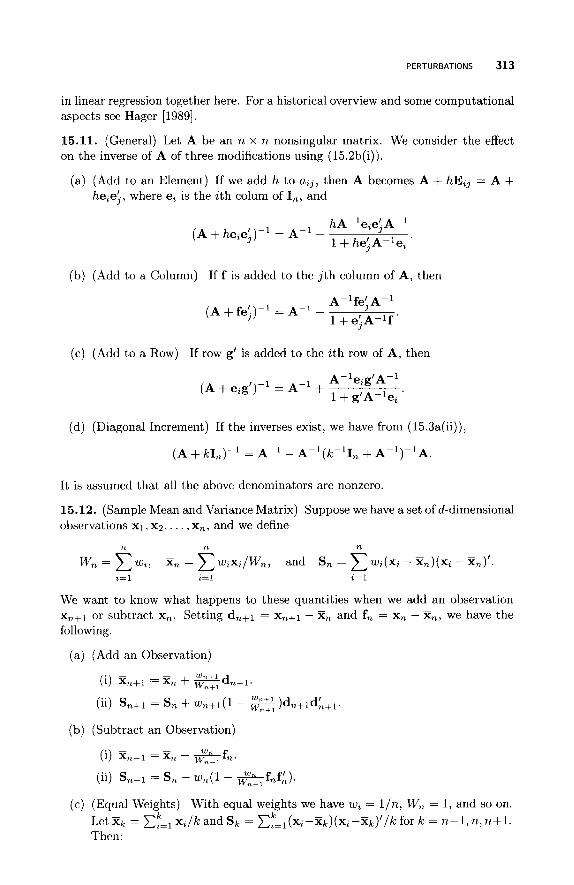
PERTURBATIONS 313
in linear regression together here. For a historical overview and some computational aspects see Hager [1989].
15.11. (General) Let A be an n x n nonsingular matrix. We consider the effect on the inverse of A of three modifications using (15.2b(i)).
(a) (Add to an Element) If we add h to a,,, then A becomes A + hE,, = A + he,ej, where e, is the ith colum of I,, and
(b) (Add to a Column) I f f is added to the j t h column of A, then
A- ' fej A-
1 + e$A-'f ' (A + fei)-' = A-' -
(c) (Add to a Row) If row g' is added to the i th row of A, then
'A-1 (A + eig')-' = A-' + ag .
1 + g'A-lei
(d) (Diagonal Increment) If the inverses exist, we have from (15,3a(ii)),
(A + kin)-' = A-' - A-'(K'I, + A-')-'A.
It is assumed that all the above denominators are nonzero.
15.12. (Sample Mean and Variance Matrix) Suppose we have a set of d-dimensional observations XI, x2,. . . , x,, and we define
n n n
W, = c w,, X, = w,x,/W,, and S, = 1 w,(x, - X,)(x, - X,)'
We want to know what happens to these quantities when we add an observation x,+1 or subtract x,. Setting d,+l = x,+1 - x, and f, = x, - x,, we have the following.
z= 1 ,=1 2= 1
- -
(a) (Add an Observation)
W , + l ( i ) %+I = X n + G d n + l .
(ii) Sn+l = S n + wn+l(l- *)dn+14+1
(b) (Subtract an Observation)
(i) %,-I = X, -
(ii) Sn-l = S, - wn(1 - A f W,_l f ' ) n '
w L
(c) (Equal Weights) With equal weights we have w, = l / n , W, = 1, and so on. Let %k = c,"=, x,/k and s k = ~,"=l(Xz-~k)(xz-X~)'/k for k = n-1,72,12+1. Then:
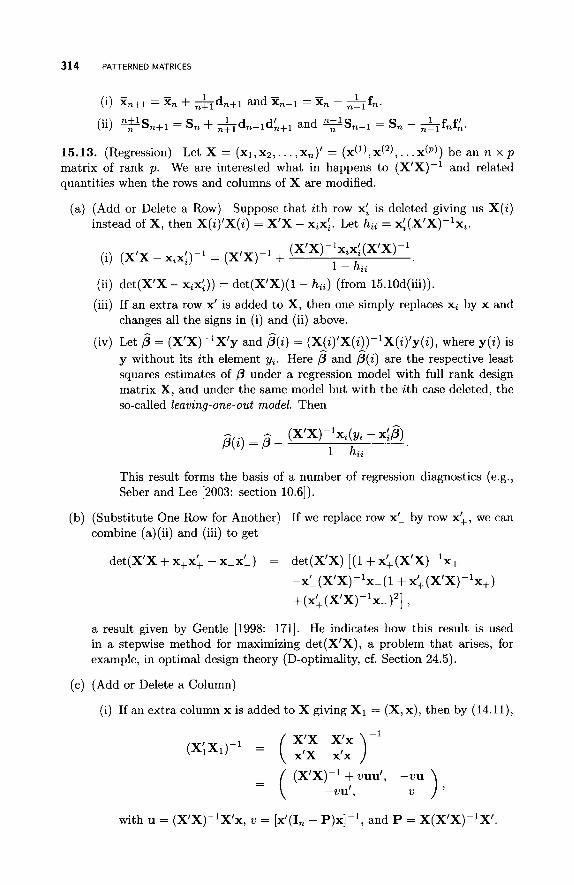
314 PATTERNED MATRICES
- (i) X,+1 = X, + &d,+l and X,-l = x, - Af,.
(ii) *S,+1 = S , + &d,+ld;+’ and %Sn-l = S, - &f,f;.
15.13. (Regression) Let X = (XI, x2,. . . , x,)’ = (x(l) , x ( ~ ) , . . .,(PI) be an n x p matrix of rank p . We are interested what in happens to (X’X)-’ and related quantities when the rows and columns of X are modified.
(a) (Add or Delete a Row) Suppose that i th row xi is deleted giving us X(i) instead of X, then X(i)’X(i) = X’X - xixi. Let hii = x:(X’X)-’xi.
(X’X) -1xix: (X’X) -1 (i) (X’X - xix:)-’ = ( X ’ X ) ~ ‘ +
1 - hii
(ii) det(X’X - xixi)) = det(X’X)(l - hit) (from 15.10d(iii)).
(iii) If an extra row x‘ is added to X, then one simply replaces xi by x and changes all the signs in (i) and (ii) above.
(iv) Let f i = (X’X)-’X’y and p^(i) = (X(i)’X(i))-’X(i)’y(i), where y(i) is y without its i th element yi. Here p and fi(i) are the respective least squares estimates of p under a regression model with full rank design matrix X, and under the same model but with the i th case deleted, the so-called leaving-one-out model. Then
A
(X’X)-’xz(yz - x p ) f i ( 2 ) = p -
1 - hii
This result forms the basis of a number of regression diagnostics (e.g., Seber and Lee [2003: section 10.61).
(b) (Substitute One Row for Another) If we replace row x’ by row x;, we can combine (a)(ii) and (iii) to get
det(X‘X + x+x: - x-x’) = det(X’X) [(1+ x:(X’X)-’x+
-x’ (X’X) -1x- (1 + x; (X’X) -‘x+)
+(x\ (X’X) -‘x-)2] ,
a result given by Gentle [1998: 1711. He indicates how this result is used in a stepwise method for maximizing det(X’X), a problem that arises, for example, in optimal design theory (D-optimality, cf. Section 24.5).
(c) (Add or Delete a Column)
(i) If an extra column x is added to X giving X1 = (X, x), then by (14.11),
= ( (X’X)-1+vuu’, -vu‘,
with u = (X’X)-’X’x, v = [x’(I, - P)x]-l, and P = X(X’X)-’X’
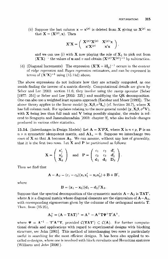
PERTURBATIONS 315
(ii) Suppose the last column x = x(P) is deleted from X giving us X(P) so that X = (X(P),x). Then
,’X(P) ) ’ ( X(P)’X(P) X(P)IX x’x =
and we can use (i) with X now playing the role of X1 to pick out from (X’X)-’ the values of u and w and obtain (X(P)’X(P))-’ by subtraction.
(d) (Diagonal Increments) The expression (X’X + kIP)-’ occurs in the context of ridge regression and Bayes regression estimators, and can be expressed in terms of (X’X)-’ using (15.11d) above.
The above expressions do not indicate how they are actually computed, as one avoids finding the inverse of a matrix directly. Computational details are given by Seber and Lee [2003: section 11.6; they involve using the sweep operator (Seber [1977: 3511 or Seber and Lee [2003: 3351) and modifiying the QR decomposition. One can also use a weighted least squares approach (Escobar and Moser [1993]). The above theory applies to the linear model (y, Xp, a21,) (cf. Section 20.7), where X has full column rank. For updates relating to the more general model (y, Xp, c2V), with X being less than full rank and V being possibly singular, the reader is ref- ered to Sengupta and Jammalamadaka [2003: chapter 91, who also include changes produced in various other statistics.
15.14. (Interchanges in Design Models) Let A = X’PX, where X is n x p , P is an n x n symmetric idempotent matrix, and Al, = 0. Suppose we interchange two rows of X so that A becomes A2. We can assume, without any loss of generality, that it is the first two rows. Let X and P be partitioned as follows:
c2 d:
x3 dl d2 D3 X = ( zi ) and P = ( zi c3 dh ) .
Then we find that
A - A2 = ( ~ 1 - C ~ ) ( X ~ X ; - x~x;) + B + B’,
where B = (XI - xz)(dl - dz)’X3.
Suppose that the spectral decomposition of the symmetric matrix A - A2 is TAT’, where A is a diagonal matrix whose diagonal elements are the eigenvalues of A-A2, with corresponding eigenvectors given by the columns of the orthogonal matrix T. Then, from (15.25),
A t = (A - TAT)’ = A’ + A+T@+T’A+,
where @ = A-’ - T’A+T, provided C(TAT’) c C(A). For further computa- tional details and applications with regard to experimental designs with blocking structure, see John [200l]. This method of interchanging two rows is particularly useful in searching for the most efficient designs. It has been also applied to so- called a-designs, where one is involved with block circulants and Hermitian matrices (Williams and John [ZOOO]).
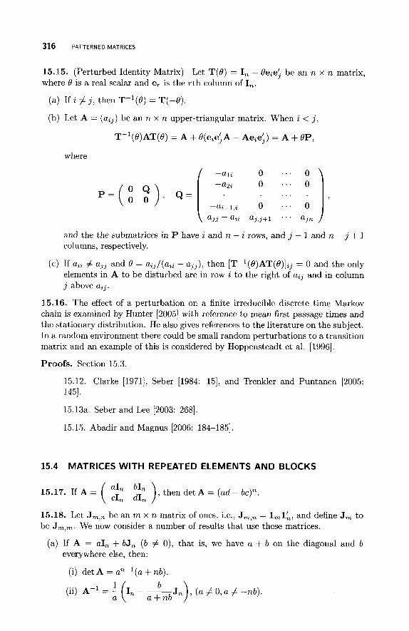
316 PATTERNED MATRICES
15.15. (Perturbed Identity Matrix) Let T(8) = I, - 0eiei be an n x n matrix, where 0 is a real scalar and e, is the rth column of I,.
(a) If i # j, then T-'(0) = T(-0).
(b) Let A = (a i3) be an n x n upper-triangular matrix. When i < j,
T-'(B)AT(O) = A + 8(eieiA - Aeieg) = A + OP,
where
and the the submatrices in P have z and n - z rows, and 3 - 1 and n - 3 + 1 columns, respectively.
(c) If a,, # a3, and 0 = az3/(azz - a,,), then [T-1(0)AT(8)],, = 0 and the only elements in A to be disturbed are in row i to the right of aZ3 and in column 3 above az3.
15.16. The effect of a perturbation on a finite irreducible discrete time Markov chain is examined by Hunter [a0051 with reference to mean first passage times and the stationary distribution. He also gives references to the literature on the subject. In a random environment there could be small random perturbations to a transition matrix and an example of this is considered by Hoppensteadt et al. [1996].
Proofs. Section 15.3
15.12. Clarke [1971], Seber [1984: 151, and Trenkler and Puntanen [2005: 1451.
15.13a. Seber and Lee [2003: 2681.
15.15. Abadir and Magnus [2006: 184-1851,
15.4 MATRICES W I T H REPEATED ELEMENTS AND BLOCKS
15.17. If A = ( :ir El ), then det A = (ad -
15.18. Let J m , , be an m x n matrix of ones, i.e., J,,, = l,l~, and define J , to be Jm,m. We now consider a number of results that use these matrices.
(a) If A = a I , + bJ, ( b # 0 ) , that is, we have a + b on the diagonal and b everywhere else, then:
(i) det A = an-'(a + nb) .
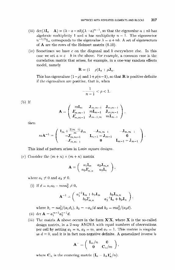
MATRICES WITH REPEATED ELEMENTS AND BLOCKS 317
(iii) det(X1,-A) = (X-~-nb)(X-a)" -~ , so that the eigenvalueafnb has algebraic multiplicity 1 and a has multiplicity n - 1. The eigenvector n- 'I2ln corresponds to the eigenvalue X = a + nb. A set of eigenvectors of A are the rows of the Helmert matrix (8.10).
(iv) Sometimes we have c on the diagonal and b everywhere else. In this case we set a = c - b in the above. For example, a common case is the correlation matrix that arises, for example, in a one-way random effects model, namely
R = (1 - p)In + pJn.
This has eigenvalues (1 - p ) and 1 +p(n- l), so that R is positive definite if the eigenvalues are positive, that is, when
1
n - 1 < p < l -~
(b) If
then
This kind of pattern arises in Latin square designs.
(c) Consider the (m + n) x (m + n) matrix
where a1 # 0 and a3 # 0.
(i) If d = ~ 1 ~ 3 - mnuz # 0,
-1
where b l = na;/(aldl), b2 = -a2/d and b3 = ma;/(asd).
(ii) det A = ay-'a;-'d.
(iii) The matrix A above occurs in the form X'X, where X is the so-called design matrix, in a 2-way ANOVA with equal numbers of observations per cell by setting a1 = n, a3 = m, and a2 = 1. This matrix is singular as d = 0, and it is in fact non-negative definite. A generalized inverse is
where C , is the centering matrix (I, - ln16/n).
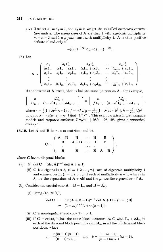
318 PATTERNED MATRICES
(iv) If we set a1 = a3 = 1, and a2 = p, we get the so-called intraclass correla- tion matrix. The eigenvalues of A are then 1 with algebraic multiplicity m + n - 2 and 1 f p f i , each with multiplicity 1. A is then positive definite if and only if
-(mn)-'/2 < p < (mn)-1/2.
(d) Let
. . . a21, b21, + c2Jm b31, + c3Jm . . . b,I, + c,J,
a n l m b,I, + c,J, d,I, + enJm ... y,I, + z,J,
b l L P l f 1;-1
f L - 1 (9 - h ) L i + hJn-1
If the inverse of A exists, then it has the same pattern as A. For example,
b l , - ~ (C - d)I,-i + dJ,-1
wheree= k[1+Xb2(n-1)], f = - X b , g = &[1-X(ad-b2)],h= &X(b2- ad) , and X = (a(c-d)+(n-l)(ad-b')))-'. This example arises in Latin square models and response surfaces; Graybill [1983: 195-1961 gives a numerical example.
15.19. Let A and B be m x m matrices, and let
/ A + B B . . . B B l
I ' B A + B . . . B B . . . .
B . . . B A + B /
where C has n diagonal blocks.
(a) (i) det C = (det A),-' det(A + nB).
(ii) C has eigenvalues X i (i = 1 ' 2 , . . . , m) each of algebraic multiplicity 1 and eigenvalues pi (i = I , 2, . . . , m) each of multiplicity n - 1, where the X i are the eigenvalues of A + n B and the pi are the eigenvalues of A.
(b) Consider the special case A + B = I, and B = J,.
(i) Using (15.18a(i)),
= det C det(A + B - B),-' det[A + B + (n - l )B] = (1 - m)"-l[1 + m(n - l ) ] .
(ii) C is nonsingular if and only if rn > 1.
(iii) If C-' exists, it has the same block structure as C with I, + aJ, in each of the diagonal block positions and bJ, in all the off-diagonal block positions, where
m(m - l ) ( n - 1) (n - 1)m + 1
-(m - 1) (72 - 1)m + 1
a = and b = (m - 1).
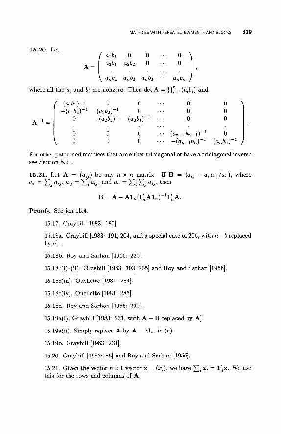
MATRICES WITH REPEATED ELEMENTS AND BLOCKS 319
15.20. Let albl 0 0 . . . ~ 2 b 1 ~ 2 b 2 0 . . .
A = ( . . . . anbl anb2 anb3 . . . anbn
where all the a, and b, are nonzero. Then det A = n~==,(a ,b , ) and
0 0
. . . 0 0 0
0 (an bn )
. . . 0 - ( ~ z b 3 ) - ~ ( ~ 3 6 3 ) ~ ~ . . . 0
. . . 0 0 0 . . . (an-lbn-l)-' 0 0 0 . . . -(an-1bn)-'
and a = C, C, aZ3, then
A-' =
For other patterned matrices that are either tridiagonal or have a tridiagonal inverse see Section 8.11.
15.21. Let A = ( a z j ) be any n x n matrix. If B = (az3 - a, a 3 / a ), where a, = Cp23, a3 = Cza231
B = A - Aln(lkAln)- '1LA.
Proofs. Section 15.4.
15.17. Graybill [1983: 1851.
15.18a. Graybill [1983: 191, 204, and a special case of 206, with a - b replaced by 4. 15.18b. Roy and Sarhan [1956: 2301.
15.18c(i)-(ii). Graybill [1983: 193, 2051 and Roy and Sarhan [1956].
15.18c(iii). Ouellette [1981: 2841.
15.18c(iv). Ouellette [1981: 2851.
15.18d. Roy and Sarhan [1956: 2301.
15.19a(i). Graybill [1983: 231, with A - B replaced by A].
15.19a(ii). Simply replace A by A - XI, in (a).
15.19b. Graybill [1983: 2311.
15.20. Graybill [1983:186] and Roy and Sarhan [1956].
15.21. Given the vector n x 1 vector x = (x,), we have C, z, = 1;x. We use this for the rows and columns of A.
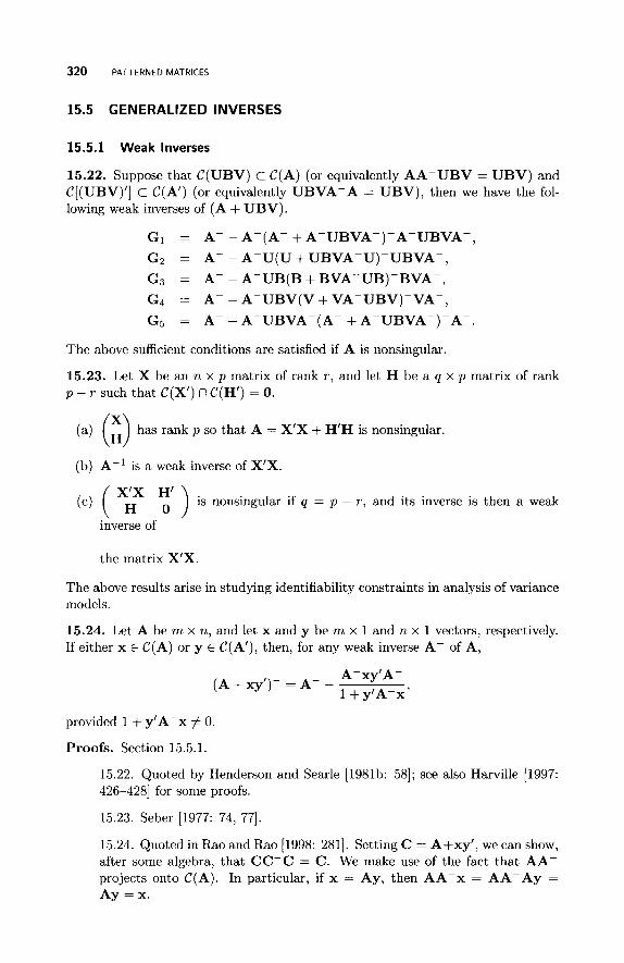
320 PATTERNED MATRICES
15.5 GENERALIZED INVERSES
15.5.1 Weak Inverses
15.22. Suppose that C(UBV) C C(A) (or equivalently AA-UBV = UBV) and C[(UBV)’] C C(A’) (or equivalently UBVA-A = UBV), then we have the fol- lowing weak inverses of (A + UBV).
GI = A- - A-(A- + A-UBVA-)-A-UBVA-,
Gz = A- - A-U(U + UBVA-U)-UBVA-,
G3 = A- - A-UB(B + BVA-UB)-BVA-, G4 = A- - A-UBV(V + VA-UBV)-VA-,
G5 = A- - A-UBVA-(A- + A-UBVA-)-A-.
The above sufficient conditions are satisfied if A is nonsingular.
15.23. Let X be an n x p matrix of rank r , and let H be a q x p matrix of rank p - r such that C(X’) n C(H’) = 0.
(a) (E) has rank p so that A = X’X + H‘H is nonsingular.
(b) A-’ is a weak inverse of X’X
(c) ( :‘ ) is nonsingular if q = p - r , and its inverse is then a weak
inverse of
the matrix X’X
The above results arise in studying identifiability constraints in analysis of variance models.
15.24. Let A be m x n, and let x and y be m x 1 and n x 1 vectors, respectively. If either x E C(A) or y E C(A’), then, for any weak inverse A- of A,
A-xy’A- 1 + y‘A-x
(A + xy’)- = A- -
provided 1 + y‘A-x # 0.
Proofs. Section 15.5.1.
15.22. Quoted by Henderson and Searle [1981b: 581; see also Harville [1997: 426-4281 for some proofs.
15.23. Seber [1977: 74, 771.
15.24. Quoted in Rao and Rao [1998: 2811. Setting C = A+xy‘, we can show, after some algebra, that CC-C = C . We make use of the fact that AA- projects onto C(A). In particular, if x = Ay, then AA-x = AA-Ay = Ay = X.
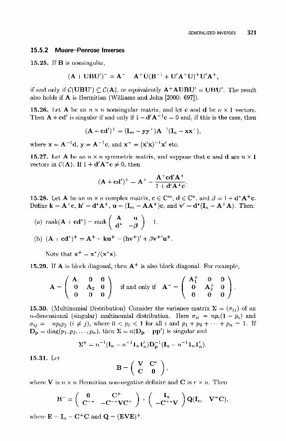
GENERALIZED INVERSES 321
15.5.2 Moore-Penrose Inverses
15.25. If B is nonsingular,
(A + UBU')' = A+ - A+U(B-' + U'A+U)+U'A+,
if and only if C(UBU') 2 C(A), or equivalently A+AUBU' = UBU'. The result also holds if A is Hermitian (Williams and John [2000: 6971).
15.26. Let A be an n x n nonsingular matrix, and let c and d be n x 1 vectors. Then A + cd' is singular if and only if 1 + d'A-'c = 0 and, if this is the case, then
(A + cd')+ = (I, - yy+)A-'(I, - xx'),
where x = A-'d, y = A-lc, and xf = (x'x)-'x' etc.
15.27. Let A be an n x n symmetric matrix, and suppose that c and d are n x 1 vectors in C(A). If 1 + d'A+c # 0, then
A+cd'A+ 1 + d'A+c '
(A + cd')' = A+ -
15.28. Let A be an m x n complex matrix, c 6 P, d 6 @", and p = 1 + d*A+c. Define k = A+c, h' = d*A+, u = (I, - AA+)c, and v' = d*(In - A+A). Then:
(a) rank(A + cd*) = rank (d". -;;)-l.
(b) (A + cd*)+ = A+ - ku' - (hv')' + pv+'u+.
Note that x+ = x*/(x*x).
15.29. If A is block diagonal, then A+ is also block diagonal. For example,
0 0 A: 0 A = ( 8' 2 0) if and only if A+ = ( X ;$ i ) .
15.30. (Multinomial Distribution) Consider the variance matrix X = (oZ j ) of an n-dimensional (singular) multinomial distribution. Here oz, = npt( 1 - p z ) and oz3 = -np,p, ( i # j ) , where 0 < p , < 1 for all i and p l + p2 + . . . + p , = 1. If D, = diag(pl,pz,. . . ,p,), then Z = n(D, - pp') is singular and
Z+ = n-'(I, - n-'l,l~)D;'(I, - n-'1 R 1' n ' )
15.31. Let v c*
B = ( c o ) , where V is n x n Hermitian non-negative definite and C is T x n. Then
where E = I, - C+C and Q = (EVE)+.
322 PATTERNED MATRICES
Proofs. Section 15.5.2.
15.25. John [2001: 11751.
15.26. Schott [2005: 197-1981
15.27. Quoted by Schott [2005: 217, exercise 5.321. Can be proved in a manner similar to that of (15.24).
15.28. Campbell and Meyer [1979: 47-48]. They also list several special cases in which one or more of u, v, and /3 are zero. They also give Moore-Penrose
inverses of
15.30. Follows from (15.26) above, along with D;'p = 1,.
15.31. Campbell and Meyer [1979: 641.
CHAPTER 16
FACTORIZATION OF MATRICES
The factorization of a matrix A can be expressed two ways; either as a reduction XAY = C or as a factorization A = URV. In many cases these are equivalent because of the presence of nonsingular matrices-for example, A = X-lCY-l if X and Y are nonsingular. Authors tend to have different preferences for which form they use. Useful summaries of some of the factorizations are given by Abadir and Magnus [2005: 1581, Horn and Johnson [1985: 1571, and Rao and Rao [1998: 190-1931.
16.1 SIMILARITY REDUCTIONS
As eigenvalues are used in this section, we remind the reader of Definition 6.1. In what follows, we assume that an n x n matrix has eigenvalues XI, A 2 , . . . , A, with lAl l 2 1x21 2 . . . 2 IA,I 2 0 and has distinct eigenvalues p1, p2, . . . , pS, similarly ordered, with algebraic and geometric multiplicities m ( p j ) and g ( p j ) , respectively.
Definition 16.1. Let A and B be n x n matrices over F. We say that A is similar to B if there exists a nonsingular matrix K over F such that K-lAK = B.
16.1. Let A be an n x n real or complex matrix.
(a) A is similar to its transpose.
(b) A*A is similar to AA'
A Matrix Handbook for Statistacians. By George A. F. Seber Copyright @ 2008 John Wiley & Sons, Inc.
323
324 FACTORIZATION OF MATRICES
(c) AA is similar to AX.
(d) A is similar to a symmetric matrix.
(e) A is similar to a complex triangular matrix (either upper or lower) whose diagonal elements are the eigenvalues of A.
16.2. Let A and B be real n x n matrices. If R is a complex nonsingular matrix such that R-IAR = B, then there exists a real nonsingular matrix S such that S-lAS = B.
16.3. Let A be an upper-triangular matrix with distinct diagonal elements diag(A). Then there exists a unit upper-triangular matrix R (i.e., with ones on the diagonal) such that R-lAR = diag(A).
Definition 16.2. Let Jm(X) be an m x m matrix of the form
x 1 0 ." 0 0
Jm(x) = [ 0 ? ! : : : 0 0 1 , 0 0 0 ." x 1 0 0 0 ." 0 X
where Jl(X) = A. Then Jm(X) is said to be a Jordan block matrix . We find it convenient to include the case m = 1.
16.4. Every Jordan block J m ( X ) (m > 1) is not diagonalizable because it has only one linearly independent eigenvector x = (zl,O,. . . ,O) ' , where z1 is arbitrary (cf. Definition 16.3 above (16.10)). This follows from the fact the diagonal elements of the upper-triangular matrix Jm(X) are its eigenvalues, so that it has one eigenvalue X repeated m times, and x satisfies Jm(X)x = Ax.
16.5. Every Jordan block is permutation similar to its transpose since Jm(X)' = IIJ,(X)II, where II = (em,em-l, . . . , e l ) is the backward identity permutation matrix, where (el,eZ,. . . ,em) = I,.
16.6. Let x = (xi) be an m x 1 vector. The Jordan block J = Jm(0) has the following properties.
(a) J x = ( x z , 2 3 , . . . ,xm,O)', representing a forward shzfi.
(b) J'x = (01x1,x2,. . . , x,-1)', representing a backward shzft.
(c) (L- J')x= (x1,~~-51,23-~~,...~2,--,-1)', representing a dzfference operator.
(d) (I, - J')-'x = ( 5 1 , 5 1 + ~ 2 , 5 1 + zz + 2 3 , . . . , z1 + 2 2 + . . . + x,)', which can be called a partial sum operator.
16.7. (Jordan Canonical Form) If A is a real or complex n x n matrix, then there exists a nonsingular matrix R such that
SIMILARITY REDUCTIONS 325
where E:=l ni = n and the X i are the (not necessarily distinct) eigenvalues of A; that is, A is similar t o Jo. The matrix JO is said to be in Jordan canonical forrn, which is unique apart from the order of the blocks. One application of the Jordan canonical form is in the analysis of a system of ordinary differential equations with constant coefficients (Horn and Johnson [1985: 132-1331). The topic of Jordan chains is considered by Abadir and Magnus [2005: section 7.61
If p1, p2 , . . . , ps are the distinct Xi , then we have the following.
(a) The number k of Jordan blocks (including multiple occurrences of the same blocks) is the number of linearly independent eigenvectors of Jo.
(b) The matrix JO is diagonalizable (cf. Definition 16.3 above (16.10)) if and only if k = n.
(c) The number of Jordan blocks correponding to pJ is the geometric multiplicity g ( p j ) . The sum of the orders (sizes) of all the Jordan blocks corresponding to pJ is the algebraic multiplicity m ( p j ) .
(d) JO is not completely determined in general by a knowledge of the eigenvalues and their algebraic and geometric multiplicities. We must also know the sizes of the Jordan blocks corresponding to each Xi .
(e) The minimal polynomial of JO (and therefore of A, as similar matrices have the same minimal polynomial, cf. (6.12)) is
S
f ( P ) = l - I ( P - 1
j = 1
where rj is the order of the largest Jordan block of JO corresponding to p j .
(f) The sizes of the Jordan blocks corresponding to a given pj are determined by a knowledge of the ranks of certain powers.
(g) If A is a real matrix with only real eigenvalues, then the similarity matrix R can be taken to be real.
(h) It is convenient to standardize the order of the Jordan blocks as follows. For each pj we have g ( p j ) blocks that we order in decreasing size, and we order these s groups of blocks according to our convention lpl I > . . . > Ips[; JO is then unique.
16.8. If A and B are n x n similar matrices, then they have the same Jordan canonical form.
16.9. Let A be an n x n upper-triangular matrix with zeros on the main diagonal (sometimes called a strictly upper-triangular matrix) .
(a) There exists a nonsingular n x n matrix S and integers n1, n2,. . . , n, with nl 2 722 2 . . . 2 n, and n1 + n 2 + . . . + n, = n such that
326 FACTORIZATION OF MATRICES
(b) If A is nilpotent with nilpotency index k , then m = dimN(A) , the size of the largest block is k x k , and each block is nilpotent.
Definition 16.3. If A is similar to a diagonal matrix, then A is said to be dzag- onalzzable. Other terms used are dzagonable, szmple, sernz-szrnple or nondefectzve. Note that A can be real or complex.
16.10. A is diagonalizable if and only if one, and hence all, of the following equiv- alent conditions are satisfied (cf. Definition 6.1):
(1) m(p.,) = g(p.,) for each j ; that is, the eigenvalues of A are all regular
(2) g(p l )+g (pz )+ . . .+g (p , ) = n , that is thesumoftheeigenspacesofAisCn.
(3) rank(A - p.,In) = n - m(p.,) for j = 1 , 2 , . . . , s. The equivalence with (1) follows from (6.lb)
(4) A possesses n linearly independent right (respectively left) eigenvectors.
16.11. If A has n distinct eigenvalues, then they are simple and therefore regular, so that by (16.10(1)) above A is diagonalizable.
16.12. A matrix A is diagonalizable if and only if h(A) = 0 , where
h(z) = (z-pl)(z-p2)...(z-p~),
and the p., are the distinct eigenvalues of A. If h(A) = 0, then h(X) = q(X) , the minimal polynomial.
16.13. It follows from (16.12) above that an idempotent matrix A is diagonalizable since h(A) = 0, where
and the eigenvalues of A are X = 0 , l .
16.14. (Product) Suppose A and B are n x n Hermitian matrices with A positive- definite. Then AB has real eigenvalues and is diagonalizable. Also, A B has the same number of positive, negative, and zero eigenvalues as B. Furthermore, any diagonalizable matrix with real eigenvalues is the product of a positive definite Hermitian matrix and a Hermitian matrix.
16.15. (Approximation) Let A = (u t J ) be an n x n matrix. For every E > 0, there exists a matrix A(€) = (u t J (c ) ) with distinct eigenvalues (and is therefore diagonalizable) such that
h ( z ) = z(z - l),
n n
i=l jzl
16.16. Let A be n x n and B be m x m matrices, and let
A 0 c = ( o € 3 )
Then C is diagonalizable if and only if A and B are both diagonalizable.
SIMILARITY REDUCTIONS 327
16.17. (Spectral Decomposition) Suppose A is diagonalizable of rank r .
(a) There exist linearly independent right eigenvectors X I , x2, . . . , x, and linearly independent left eigenvectors yi, yh, . . . , yk such that yixj = bij , where bij = 1 when i = j and 0 otherwise. Also
n
i= 1 n
i=l
for nonzero Xi , where the rank one Fi are not unique unless all the eigen- values are distinct. Here the Fi are idempotent, mutually orthogonal, and CYTIFi = I,. If R = (x1,x2,. . . ,x,) and S = (y1,y2,. . . ,yn)', then A = RAS, where SR = I, implies that S = R-l. Note that as the rank is unchanged when multiplying by a nonsingular matrix, rank A = rank A, and rank A is the number of nonzero eigenvalues of A.
(b) (Unique Decomposition)
(i) We can also write S
A = CPLjEj, j=1
where Ej represents the sum of the Fi corresponding to the same eigen- value and the pj are the distinct eigenvalues (including zero). The Ej, called the spectral set, are unique, idempotent, and mutually orthogonal (i.e., EjEk = 6jkEj) and satisfy Cg,, Ej = I,.
(ii) Also, for k = 1 , 2 , . . . ,
j = 1
(c) If A is nonsingular, then
If A is singular, then
where the summation is over the nonzero eigenvalues, and A+ is the Moore- Penrose inverse of A. This is proved directly from the definition of A+.
For a spectral decomposition of an arbitrary matrix see Rao and Mitra [1971: 381.
328 FACTORIZATION OF MATRICES
16.18. Suppose A is an n x n diagonalizable matrix with distinct eigenvalues X i . Then the Vandermonde matrix (cf. Section 8.12.1)
1 . . . ...
B = . . .
A;-1 . . . A2-1
is nonsingular with inverse B-’ = (&), say. From the previous result (16.17b), with s = n and Ej = Fj, we have
where “18” is the Knonecker product. Now B @ I, can be expressed symbolically as (bijI,) so that using (B @ In)-1 = B-’ 8 I, and defining A’ = I, we have
n
j=1
Substituting in Ak from (16.17b(ii)) gives us
n n
16.19. If A is real symmetric (respectively Hermitian) n x n matrix with distinct eigenvalues pj ( j = 1 ,2 , . . . , s), then m ( p j ) = g ( p j ) for j = 1,2, . . . , s. Hence, by (16.10( 1)) above, all real symmetric (respectively Hermitian) matrices are diagc- nalizable.
Proofs. Section 16.1.
16.la. Horn and Johnson [1985: 134-1351, Meyer [2000a: 5961, and Zhang [1999: 831.
16.lb-c. Zhang [1999: 831.
16.1d. Quoted by Rao and Rao [1998: 1921
16.le. Rao and Bhimasankaram [2000: 288-2891
16.2. Zhang [1999: 1521
16.3. Abadir and Magnus [2006: 1861.
16.5. Horn and Johnson [1985: 1341.
16.6. Abadir and Magnus [2005: 1931.
REDUCTION BY ELEMENTARY TRANSFORMATIONS 329
16.7. For proofs, section 7.51, Horn and 7.81, and Rao
references, and comments see Abadir and Magnus [2005: and Johnson [1985: section 3.11, Meyer [2000a: sections 7.7
I and Bhimasankaram [2000: section 8.61.
16.8. The result follows from the uniqueness of the Jordan canonical form.
16.9a. Abadir and Magnus [2005: 195-1961 and Horn and Johnson [1985: 1231.
16.9b. Meyer[2000a: 5791.
16.10. Rao and Bhimasankaram [2000: 296-2971.
16.11. Horn and Johnson [1985: 481.
16.12. Horn and Johnson [1985: 1451 and Rao and Bhimasankaram [2000: 296-2971.
16.13. Rao and Bhimasankaram [2000: 2971.
16.14. Horn and Johnson [1985: 4651.
16.15. Horn and Johnson [1985: 891.
16.16. Horn and Johnson [1985: 491.
16.17a. Harville [1997: section 21.51.
16.17b. Rao and Bhimasankaram [2000: 299-3001.
16.2 REDUCTION B Y ELEMENTARY TRANSFORMATIONS
16.2.1 Types of Transformation
Definition 16.4. An elementary row transformation of an m x n matrix A over F is one of the following operations:
Multiply row i by a scalar c in F. This achieved by left-multiplying A by the identity matrix I, with its i th diagonal element replaced by c . The latter has determinant c.
Add row j to row i. This is achieved by left-multiplying by the matrix I, + EzJ, where E,, has 1 in the ( i , j ) t h position and zeros elsewhere. This transformation has determinant 1.
Interchange the i th and j t h rows. This is achieved by left-multiplying by the permutation matrix nZJ, where IIZJ is I, with its i th and j t h rows in- terchanged. (Technically the third transformation can be carried out using a sequence of the previous two transformations, but that route is less conve- nient .)
These operations can also be extended to submatrices of partitioned matrices (cf. Zhang 1999: 301).
330 FACTORIZATION OF MATRICES
16.20. Note the following:
(a) IIij is symmetric and orthogonal so that 11,' = IIij.
(b) E:, = 0 and (I, + cE,,)-' = I, - cE,,.
Definition 16.5. An elementary (row) transformataon matrix M is defined to be one of the above three types of matrices, referred to as types ( l ) , (2), and (3). For further details see, for example, Abadir and Magnus [2005: section 6.11
Elementary column transformations can be carried out by right-multiplying A by an elementary transformation matrix (but using E,, = Ei3 instead of E,,).
16.21. The inverse of an elementary transformation matrix is also an elementary transformation matrix. Also, as such matrices are all nonsingular, a product of such matrices is nonsingular. Therefore multiplying A by such a matrix does not change the rank of A (cf. 3.14a).
16.2.2 Equivalence Relation
Definition 16.6. Let A and B be m x n real or complex matrices. If B is obtained from A by elementary row or column transformations matrices, then A is said to be equivalent to B, and we write A - B.
16.22. Any one of the following statements implies the other two.
(1) A - B .
(2) B = RAS for some non-singular matrices R and S.
(3) rankA = rankB (cf. 3.14a).
Definition 16.7. From (16.22(2)) above we see that: (i) A - A (reflexive), (ii) if A - B, then B - A (symmetric), and (iii) if A - B and B - C, then A - C (transitive). Any relation that satisfies these three conditions is called an SRT relation. Thus the equivalence relation "-" is an SRT relation.
Other SRT relations for square matrices are summarised as follows:
(1) If B = R-'AR for nonsingular R, then B is said to be similar to A. This is discussed in Section 16.1 above.
(2) If B = R'AR for nonsingular R, then B is said to be congruent t o A. Its main application is for real matrices. If A and B are complex matrices such that B = R*AR, then B is said to be Hermitian congruent t o A.
(3) If B = U*AU, where U is unitary, then B is said to be unitarily similar to A. If, for real matrices, B = T'AT, where T is orthogonal, we say that B is orthogonally similar to A.
16.2.3 Echelon Form
Definition 16.8. Using elementary row transformations, a real or complex m x n matrix A can be reduced to a matrix B with the following properties:
(1) If a row contains a t least one nonzero entry, then the first nonzero entry is 1.
REDUCTION BY ELEMENTARY TRANSFORMATIONS 331
(2) The zero rows, if any, come last.
(3) In any two consecutive nonzero rows, the leading 1 in the lower row occurs further to the right than the leading 1 in the upper row.
A matrix in the above form is said to be in (row) echelon form. For example,
0 1 * * *
B I I ( 0 0 0 0 1 * !I, 0 0 0 0 0 0
where the elements denoted * are arbitrary. If we now subtract multiples of the second and third rows from the first, we obtain
0 1 * 0 0 *
. z = ( : : ; ; ; :) 0 0 0 0 0 0
This matrix has the additional property:
(4) Each column that contains a leading 1 has zeros elsewhere.
A matrix with the above four properties is said to be in reduced (row) echelon form We shall omit the word L‘row’’ in using the above definitions. Rao and Bhi- masankaram [2000: 167-1701 give a number of algorithms for carrying out various reductions. It should be noted that the terminology relating to echelon forms is not consistent in the literature.
We see that the first three rows of Bz give a row basis for the original matrix A, and the three columns each containing 1 form a column basis for A.
16.23. Any matrix A can be reduced to a unique matrix in reduced echelon form by elementary row transformations.
16.24. The rank of a matrix in reduced echelon form is the number of nonzero rows. This is the same as the rank of the original matrix.
16.25. If A is a nonsingular matrix of order n, then its reduced echelon form is I,. Hence there exist elementary transformation matrices Mk, k = 1 , 2 , . . . , K , such that MKMK-1 . . . M I A = I,, i.e., MA = I,, where M is nonsingular. Also, taking A over to the right-hand side, MKMK-1. . . M11, = A-’. Thus any sequence of elementary row transformations that transforms A to I, transforms I, to A-I.
16.26. For any two n x p matrices A and B, the following statements are equivalent.
(1) C(A’) = C(B’).
(2) The reduced echelon forms of A and B are the same.
(3) B can be obtained from A by a finite sequence of elementary row operations.
(4) B = KA for some nonsingular matrix K.
Proofs. Section 16.2.3.
16.23. Rao and Bhimasankaram [2000: 1721.
16.26. Rao and Bhimasankaram [2000: 171-1721.
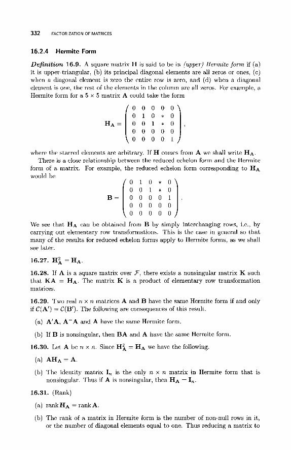
332 FACTORIZATION OF MATRICES
16.2.4 Hermite Form
Definition 16.9. A square matrix H is said to be in (upper) Hermite f o r m if (a) it is upper-triangular, (b) its principal diagonal elements are all zeros or ones, (c) when a diagonal element is zero the entire row is zero, and (d) when a diagonal element is one, the rest of the elements in the column are all zeros. For example, a Hermite form for a 5 x 5 matrix A could take the form
H A = 0 0 1 * 0 , [; ; ; ; ;] where the starred elements are arbitrary. If H comes from A we shall write HA.
There is a close relationship between the reduced echelon form and the Hermite form of a matrix. For example, the reduced echelon form corresponding to HA would be [;;;;;] We see that HA can be obtained from B by simply interchanging rows, i.e., by carrying out elementary row transformations. This is the case in general so that many of the results for reduced echelon forms apply to Hermite forms, as we shall see later.
16.27. H i = HA.
16.28. If A is a square matrix over F , there exists a nonsingular matrix K such that KA = HA. The matrix K is a product of elementary row transformation matrices.
16.29. Two real n x n matrices A and B have the same Hermite form if and only if C(A’) = C(B’). The following are consequences of this result.
B = 0 0 0 0 1 . 0 0 0 0 0
(a) A’A, A-A and A have the same Hermite form.
(b) If B is nonsingular, then B A and A have the same Hermite form.
16.30. Let A be n x n. Since H i = HA we have the following.
(a) AHA = A .
(b) The identity matrix I, is the only n x n matrix in Hermite form that is nonsingular. Thus if A is nonsingular, then HA = I,.
16.31. (Rank)
(a) rankHA = rank A.
(b) The rank of a matrix in Hermite form is the number of non-null rows in it, or the number of diagonal elements equal to one. Thus reducing a matrix to
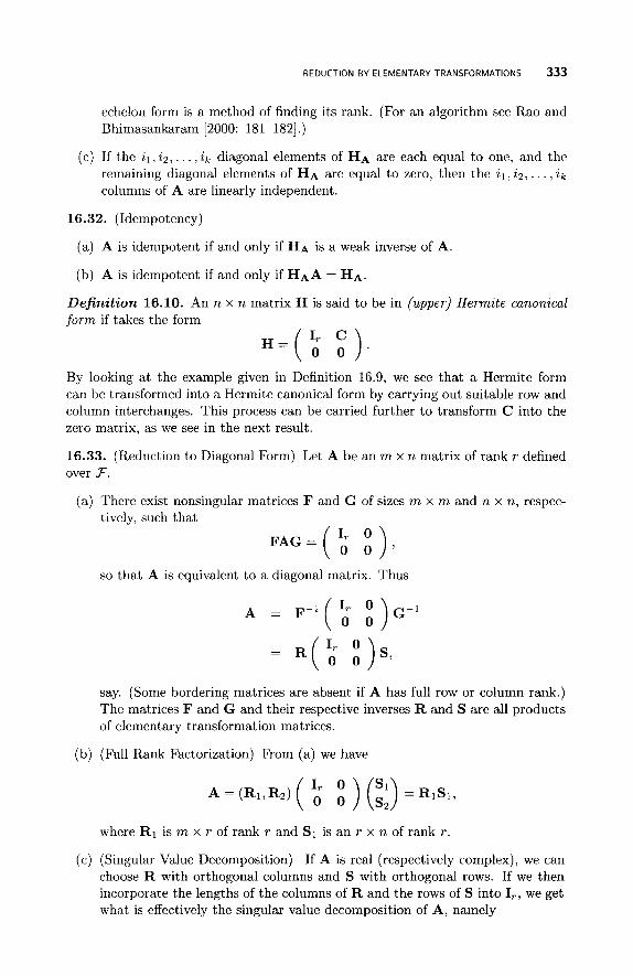
REDUCTION BY ELEMENTARY TRANSFORMATIONS 333
echelon form is a method of finding its rank. (For an algorithm see Rao and Bhimasankaram [2000: 181-1821 .)
(c) If the z l , 2 2 , . . . , z k diagonal elements of HA are each equal to one, and the remaining diagonal elements of HA are equal to zero, then the 2 1 , i 2 , . . . , ik columns of A are linearly independent.
16.32. (Idempotency )
(a) A is idempotent if and only if HA is a weak inverse of A.
(b) A is idempotent if and only if HAA = HA.
Definition 16.10. An n x n matrix H is said to be in (upper) Hermite canonical form if takes the form
By looking at the example given in Definition 16.9, we see that a Hermite form can be transformed into a Hermite canonical form by carrying out suitable row and column interchanges. This process can be carried further to transform C into the zero matrix, as we see in the next result.
16.33. (Reduction to Diagonal Form) Let A be an m x n matrix of rank r defined over F.
(a) There exist nonsingular matrices F and G of sizes m x m and n x n, respec- tively, such that
so that A is equivalent to a diagonal matrix. Thus
say. (Some bordering matrices are absent if A has full row or column rank.) The matrices F and G and their respective inverses R and S are all products of elementary transformation matrices.
(b) (Full Rank Factorization) From (a) we have
where R1 is m x r of rank r and S1 is an r x n of rank r .
(c) (Singular Value Decomposition) If A is real (respectively complex), we can choose R with orthogonal columns and S with orthogonal rows. If we then incorporate the lengths of the columns of R and the rows of S into I,, we get what is effectively the singular value decomposition of A, namely
334 FACTORIZATION OF MATRICES
where P and Q are orthogonal (respectively unitary) matrices and Dr is a diagonal matrix with positive elements. This decomposition is discussed in more detail in Section 16.3. We note that
Thus A can be expressed in the form P 2 Q 2 , where P2 has orthogonal columns and Q 2 has orthogonal rows. We can choose P2 (respectively Q 2 ) to have orthonormal columns (respectively rows).
Proofs. Section 16.2.4.
16.27. Quoted by Graybill [1983: 1311.
16.28. Graybill [1983: 1301 and Rao [1973: 181.
16.29-16.31. Graybill [1983: 138-1401.
16.32. Graybill [1983: 140-1411.
16.33a. Marsaglia and Styan [1974a: 280, theorem 101 and Rao [1973: 191.
16.33b. Marsaglia and Styan [1974a: 271, theorem 11 and Rao [1973: 191.
16.3 SINGULAR VALUE DECOMPOSITION (SVD)
The singular value decomposition is regarded by many as one of the most useful factorizations for real or complex matrices. For example, the SVD has many ap- plications in statistics such as SAS (single-spectrum analysis) in times series (cf. Golyandina et al. [2001: chapter 4]), matrix approximation in dimension reduction techniques, least squares approximation of a square matrix by a scalar multiple of an orthogonal or unitary matrix (Horn and Johnson [1985: 4291, and procrustes analysis (Gower and Dijksterhuis [2004] and Seber [1984: section 5.61). It is also a useful computational tool for calculating various quantities. In what follows, we interpret the transpose as conjugate transpose when dealing with complex matrices.
Definition 16.11. Any m x n real (respectively complex) matrix of rank T (T 5 p = min{m, n} ) can be expressed in the form
Amxn = P m x m x m x n Q h x n r
where P is an m x m orthogonal (respectively unitary) matrix, Q is an n x n orthogonal (respectively unitary) matrix, and X = (uzJ) is an m x n matrix with
SINGULAR VALUE DECOMPOSITION (SVD) 335
This factorization of A is called the singular value decomposition. The uii, abbre- viated to C T ~ = ui(A) ( i = 1,2, . . . , p ) , are called the singular values of A, which are defined to be the positive square roots of the ranked eigenvalues of AA’. These eigenvalues are non-negative as AA’ is non-negative definite (by 10.10).
The columns of p i of P are the orthonormalized right eigenvectors associated with AA’, and the columns qi of Q are the orthonormalized right eigenvectors associated with A’A. The first r columns in each case correspond to the nonzero C T ~ . Note that Aqi = uip i and A ’ p i = uiqi (i = 1 ,2 , . . . , T ) . The vectors p i and qi are also called the left and right singular vectors, respectively, associated with ui.
We note that AA’ and A’A have p common eigenvalues (cf. 6.54c), including some zeros when r < p. Any remaining eigenvalues of AA’ (if m > n) or A’A (if m < n) are zero.
Existence proofs are given by Horn and Johnson [1985: 4111, Rao and Rao [1998: 172, complex case], Schott [2005: 140-141, real case], Searle [1982: 316, real case], and Seber and Lee [2003: 471, real case]. For some computational details see Gentle [1998: section 4.41, Golub and Van Loan [1996], and Stewart [1998, 20011.
In practice, several versions of the SVD are given in the literature, which we give below.
(1) Let A p = d i a g ( u l , u z , . . . , u ~ ) . I f p = n < m , then
A = P (:) Q’ = P,A,Q’,
where the m x n matrix P, consists of the first n columns of P, and A, and Q are both n x n. The zero matrix is omitted if m = n. If p = m < n, then
A = P(Am, 0)Q’ = PA,QA,
where Qm consists of the first m columns of Q. We note that PLP, = I, and QAQm = I,. These two versions are often referred to as the thin singular value decompositions.
Is the decomposition unique? If m 2 n (i.e., p = n) , then E will be unique as the eigenvalues of A’A are unique. However, the eigenvectors making up P, and Q will not be unique unless the eigenvalues are distinct and an appropriate sign convention is adopted for eigenvectors.
(2) If P = (p i j ) and Q = ( q i j ) , with respective columns p i and qi, then
and azj = c‘,=1 UkPzkqjk. If A is complex and P and Q are unitary matrices, then A = EL=, a k p k q ; and = UkpzkqJk.
Note that AA‘P, = P,AZ and A’AQ, = Q,A:. The correct procedure is to find P, and A? from AA’P, = P,AF and then define Q, = A’P,A;’. Alternatively, we can obtain Q, and A: from A’AQT = Q,A: and then define P, = AQ,A,‘ (Abadir and Magnus [2005: 2261).
336 FACTORIZATION OF MATRICES
16.34. Let A be an m x n matrix. From the above we have the following useful informat ion.
(a) The number of nonzero singular values is the rank of A. This provides a useful computational method for finding the rank of a matrix.
(b) The T columns of P, and Qr are orthonormal bases for C(A) and C(A’), respectively, while the remaining columns of P and Q span N(A’) and N ( A ) , respectively.
(c) PA = P,Pk, the orthogonal projection onto C(A).
(d) A and (A*A)l/’ have the same singular values.
(e) Two full-rank factorizations of A (cf. 3.5) are (P,A,)(QC) and (Pr)(A,Q:).
Proofs. Section 16.3.
16.34a-b. Schott [2005: 140-1411.
16.34~. Sengupta and Jammalamadaka [2003: 431.
16.34d. Follows from the fact that (A*A)’/’((A*A)’/’)* = A*A is Hermi- tian with eigenvalues .:(A).
1 6.4 T R I A N G U LA R FAC T O R I Z AT I 0 N S
16.35. ( L U and LDU factorizations) Under certain conditions, a real or complex m x n matrix can be expressed in the form A = L1U1, where L1 is lower-triangular and U1 is upper-triangular. If m < n, then L1 is m x m, while if m > n, L1 is m x n.
(a) A sufficient condition for such a factorization to exist is that for k = I , 2, . . . , p ( p = min{m,n}), each k x k leading principal submatrix Ak of A is nonsin- gular.
(i) The usual factorisation is to have either the diagonal elements of L1 all ones (and written as L), or the diagonal elements of U1 all ones (and written as U) so that
A = LU = LU.
(ii) If we put the diagonal elements from both matrices into a single diagonal matrix D, then
A = LDU.
(b) If m < n, which is often the case, and Ak is nonsingular for k = 1 , 2 , . . . , m, then A = L U , where L is m x m and nonsingular, U is an m x n matrix such that the first m columns form an upper-triangular matrix with unit diagonal elements, and L and U are unique.
(c) A typical application of the above theory is the solution of linear equations, for example Bx = b. If we set A = (B, I,, b) and then factorize A, we can
TRIANGULAR FACTORIZATIONS 337
obtain B-' as a bonus (Rao and Bhimasankaram [2000: 2131). If B is square and nonsingular and B = LU, then we can solve Ly = b for y using forward substitution and solve Ux = y for x by back substitution. The process is usually refered to as Gaussian elimination.
(d) The matrix MI, = I, - Te;, where T E IW" and eI, has 1 for its kth element and zeros elsewhere, is a Gauss transformation if the first k elements of T are zero. If this is the case, and 7i = X ~ / X I , (XI, # 0) for i = k + 1,. . . , n, then
MI,X 1 (XI, 2 2 , . . . , xk, 0 , . . . ,O) '
16.36. (Square Matrix LU Factorizations) matrix and let AI, be its leading k x k principal submatrix.
Let A be a real or complex n x n
(a) Suppose A has rank r . If AI, is nonsingular for k = 1 , 2 , . . . , r , then A may be factored as A = LU, where L and U are n x n. Furthermore, the factorization may be chosen so that either L or U is nonsingular. Both L and U can be chosen to be nonsingular if A is nonsingular (i.e., r = n).
(b) There exist n x n permutation matrices lI1 and I I 2 such that A = lI1LUII2. If A is nonsingular, it may be written as
A = II1LU.
(c) Suppose Ak is nonsingular for k = 1 , 2 , . . . , n - 1.
(i) A can be expressed in the form A = LU = LU, where all the triangular matrices are unique.
(ii) Also, A can also be expressed in the form A = LDU, where D is diagonal and all the matrices are unique. (Note that it is possible for A be singular.)
(iii) If A is a real symmetric matrix, then we can also write A = U'DIU, where U is real and the diagonal matrix D1 has elements fl.
(d) Suppose A is nonsingular and A = L U . If L = ( l t J ) , then, since det A =
de tL . de tU , we have d e t A = ny=,lZZ # 0, detAk = n,"=, l,, # 0 for k = 1 , 2 , . . . , n - 1, and L and U are unique, by (c).
form A = U*DzU, where D2 is a diagonal matrix. (e) If A is Hermitian with an LDU factorization, then we can express it in the
16.37. (Schur Decomposition Theorems) We now consider a series of powerful theorems that can be used to provide shorter proofs for a wide range of other results (e.g., Abadir and Magnus [2005: section 7.41).
Let XI, A 2 , . . . , A,, be the eigenvalues of the n x n matrix A in a prescribed order.
(a) If A is a real or complex matrix, there exists a unitary matrix Q such that Q'AQ = T is upper-triangular with diagonal elements the eigenvalues of A in the same order. Neither Q nor T are unique.
(b) If A is real with real eigenvalues, then Q can be chosen to be real and or- thogonal. The upper-triangular matrix is also real.
338 FACTORIZATION OF MATRICES
(c) If A is real with k real eigenvalues XI, Az, . . . , X I , and complex eigenvalues z, + i y , for j > k , there exists a real orthogonal T such that T’AT = R, where R resembles an upper-triangular matrix, but with diagonal blocks of the form R11,R22,. . . , Rtt. Here RJ3 = A,, for j = 1 , 2 , . . . , k ; and for j > k
where bj 2 cj and bjcj > 0. The elements below these blocks are zero so that R is of upper Hessenberg form. Golub and Van Loan [1996: 3411 refer to such a matrix as quasi-triangular and show how to compute it using QR iterations (cf. Section 16.5). For an application to probability theory see Edelman [ 19971.
16.38. (Cholesky Decomposition for Non-negative Definite Matrices) If A is an n x n non-negative definite matrix, there exist n x n upper-triangular matrices U and U1 with non-negative diagonal elements such that
A = U’U = U1Ui.
If A is positive definite, the matrix U is unique if its diagonal elements are all positive (or all negative); the same applies to U1. Some writers prefer to use lower- triangular matrices L = U’ or L1 = Ui. The result also holds for A Hermitian non-negative definite, that is, there exists an upper-triangular matrix U such that A = U*U. If A is positive definite, then U is unique if its diagonal elements are positive (Rao and Rao [1998: 1731). For some computational aspects when A is non-negative definite see Smith [2001].
16.39. A scaled version of the above when A is positive definite is also used. If D = diag(ull,u22,. . . , unn), then D has an inverse. Let
so that A = U’U fJ’D2fJ = U’DU = LDL’,
where D is a diagonal matrix with positive diagonal elements.
16.40. (Algorithm for the Cholesky Decomposition) If A is a positive definite n x n matrix, and the diagonal elements of U are all positive, we have the following steps.
Step 1: Set
ull = a’” 11 , u1j = - ( j = 2 , 3 , . . . , n). a1j
ull
Step 2: For i = 2 , 3 , . . . , p - 1 set
uzj = 0 ( j = 1 , 2 , . . . , 2- l ) ,
TRIANGULAR FACTORIZATIONS 339
2 - 1 a ~ j - c~,=l u k i u k j
uij = ( j = i + 1,. . . , n). uii
Step 3: Set n-1 112
unn = (arm - c u:i) . k = l
The decomposition A = U D U can be used to avoid the computation of square roots. This modification is called the Banachiewicz factorization or the root-free Cholesky decomposition (Gentle [1998: 93-94]).
16.41. (Matrix Inverse) If A = U’U is a positive definite n x n matrix, we have A-l = U-’(U’)-’ = TT’, where T is upper-triangular. From UT = In we find that T is given by
ti2 = u;* ( i = 1 , 2 , . . . ,n),
t , j = 0 (2 > j ) ,
Then
k=s
which is the product of the r th and sth rows of T.
Proofs. Section 16.4.
16.35a. Golub and Van Loan [1996: 1021.
16.3513. Rao and Bhimasankaram [2000: 211-2121
16.35~. Golub and Van Loan [1996: 88-1031.
16.35d. Golub and Van Loan [1996: 94-95].
16.36a. Horn and Johnson [1985: 1601
16.36b. Horn and Johnson [1985: 1631
16.36c(i). Graybill [1983: 2071 and Rao and Bhimasankaram [ZOOO: 2161
16.36c(iii). Graybill [1983: 2101.
16.36d. Golub and Van Loan [1996: 971.
340 FACTORIZATION OF MATRICES
16.37a. Abadir and Magnus [2005: 1871, Horn and Johnson [1985: 791, Rao and Rao [1998: 174-1751, Schott [2005: 1571, and Zhang [1999: 64-65].
16.3713. Muirhead [1982: 5871 and Schott [2005: 1581.
16.37~. Rao and Rao [1998: 189-1901.
16.38. For an inductive proof for the positive-definite case see Schott [2005: 1471 and Seber [1977: 3881.
16.40. Seber and Lee [2003: 3361.
16.41. Seber [1977: 305-3061,
16.5 ORTHOGONAL-TRIANGULAR REDUCTIONS
The so-called QR decomposition plays an important role in the analysis of regres- sion models, particularly in statistical computing packages. In fact, many of the regression theorems can actually be derived via the QR decomposition (e.g., Ansley [1985], Eubank and Webster [1985], Mandel [1982], and Nelder [1985]).
Definition 16.12. Any n x p real matrix A of rank r can be expressed in the form A = QR, where Q is an n x n orthogonal matrix and R is an n x p upper-triangular matrix. This is called the QR decomposition. If n 2 p , then
= QpRl,
where Qp consists of the first p columns of Q, and R1 is a p x p upper-triangular matrix. Harville [1997: 66-68], Horn and Johnson [1985: 112-1131, and Seber and Lee [2003: 3381 give algorithmic proofs, while Seber [1977: 3881 gives an inductive proof. Some authors refer to A = QpRl as the QR decomposition.
If n 5 p , we replace R by (R2, S), where R2 is an n x n upper-triangular matrix. The above results and those below are also true for complex A if Q is now unitary and we replace ’ by * (cf. Rao and Rao [1998: 1681).
Note that Q‘A = R, and the reduction of A can be carried out using a variety of algorithms. For example, the orthogonal matrix Q’ could consist of a product of Householder reflections or Givens rotations, or one could use the Gram-Schmidt algorithm. For further details of the real case see Seber and Lee [2003: chapter 111.
16.42. We use the above notation in what follows, and we assume n 2 p .
(a) Suppose T = p .
Since R1 has full rank p , A’A = RiQbQpR1 = RiR1 is positive def- inite, and RiR1 is the Cholesky decomposition of A’A. Therefore, if the diagonal elements of R1 are all positive (or all negative), then R1 is unique and Qp = ART1 is unique. Hence the decomposition A = QpRl is also unique. However, the matrix QnPp is not unique because any per- mutation of its columns will still give A = QR.
ORTHOGONAL-TRIANGULAR REDUCTIONS 341
(ii) The Moore-Penrose inverse of A is
A+ = (R;’, 0)Q’ = RT’Q’ P’
(iii) If A is n x n and nonsingular, then
n
det A = det Q det R1 = rii, i=l
where R1 = (r i j ) . This is a useful method of finding a determinant. One application in statistics is in optimal experimental designs. For example, the D-optimal criterion chooses the design matrix X such that det(X’X) is maximized.
(b) Suppose r < p .
We first note that A‘A = RiR1 as above, but now A‘A is non-negative definite. However, R’,R1 is still the Cholesky decomposition of A’A and R1 is unique if the diagonal entries are non-negative. An inductive proof for the case n = p is given by Graybill [1983: 2101.
We can permutate the columns of A by postmultiplying by a permu- tation matrix II so that the first r columns of the permutated matrix A = AII are linearly independent. Then A = QR, where
and Rll is an r x r nonsingular upper-triangular matrix. Thus R is upper-triangular, but with its bottom n - T rows all zeros. Since II-’ = II’ we have
A = QRII’
where QT consists of the first r columns of Q. As II is not unique, QT will not be unique.
A weak inverse of A is given by
R-l 0 A- =11 ( i1 ) Q’,
as AA-A = A.
Additional orthogonal transformations can be applied to A = QRII’ to
where P is orthogonal and Ro is r x r and nonsingular. This is a conve- nient method of finding r.
342 FACTORIZATION OF MATRICES
(v) From (iv), A + = P ( R,’ 0 o ) Q ’
For further computational details see Gentle [1998: 95-1021 and Golub and Van Loan [1996: section 5.21.
There is also a symmetric QR iterative process that is a useful computational tool (Golub and Van loan [1996: section 8.21).
16.43. (Tridiagonal Matrix) If T = QR is a QR decomposition of a symmetric tridiagonal matrix T, all matrices being n x n, then Q has lower bandwidth 1, R has upper bandwidth 2, and
T1 = R Q = (Q’Q)RQ = Q’TQ
is also symmetric and tridiagonal. (The upper bandwidth is the number of nonzero diagonals above the main diagonal, and the lower bandwidth is the number of nonzero diagonals below the main diagonal; all other elements except possibly those in the main diagonal are zero.) The factorization can be computed by applying a sequence of n - 1 Givens rotations.
Proofs. Section 16.5.
16.42a(ii). Bates [1983].
16.42a(iii). Gentle [1998: 1151.
16.42b(i)-(iii). Gentle [1998: 961
16.42b(iv). Gentle [1998: 1151.
16.43. Golub and Van Loan [1996: 4171.
16.6 FURTHER DIAGONAL OR TRIDIAGONAL REDUCTIONS
16.44. (Spectral Decomposition Theorem) Let A be any n x n real symmetric (respectively Hermitian) matrix. Then there exists an orthogonal (respectively unitary) matrix Q = (ql, 9 2 , . . . , q,) such that
Q’AQ = diag(Al,Al,. . . , A , ) = A, say,
where A1 2 A2 2 . . . 2 A, are the ordered eigenvalues of A (which we know are real). When A is Hermitian, Q’ is replaced by Q*. With the above ordering, A is unique and Q is unique up to a postfactor of
where k is the number of different eigenvalues of A; ml , m2, . . . , mk are the algebraic multiplicities, that is A1 = A2 = . . . = A,, > X m l + l = .. . = Amlfma, and so on;
FURTHER DIAGONAL OR TRIDIAGONAL REDUCTIONS 343
and Q(m,) stands for the set of all m, x m, orthogonal (respectively unitary) matrices.
If all the eigenvalues are distinct, each rn, = 1 and S reduces to a diagonal matrix with diagonal elements equal to f l . In this case the columns q, of Q are unique except for their signs. If we stipulate, for example, that the element of q, with the largest magnitude is positive, then S = I, and Q is unique. We note that:
(a) A = QAQ’ = C:=l X,q,qi = C:=l X,F,, where the F, are symmetric, idem- potent, and satisfy F,F, = 0 for all i , j , j # i.
(b) If x = Qy, then x’Ax = y’Q’AQy = Xly; + . . . + Any;. An algorithm for carrrying out this reduction by completing the square rather than finding eigenvalues and eigenvectors (known as Lagrange’s reduction) is described by Rao and Bhimasankaram [2000: 3331.
(c) If A has rank T , A, contains the T nonzero eigenvalues, and Q, contains the corresponding right eigenvectors of A, then A = Q,A,Q~, where QLQ, = I,.
16.45. (Tridiagonal Reduction) Suppose A is a real symmetric n x n matrix.
(a) There exists an orthogonal matrix Q such that
Q‘AQ = B,
where B is tridiagonal. This is a very useful reduction used in numerical anal- ysis because it provides an intermediate step for speeding up a diagonalization process. If Q = ( q l , q Z , . . . ,q,), then the qi are called Lanczos vectors (cf. Golub and Van Loan [1996: 4731)
(b) If ql is defined in (a), then
where R is upper-triangular. The matrix in brackets is a Krylov matrix. If R is nonsingular, then B of (a) has no zero subdiagonal elements.
16.46. (Normal Matrix)
(a) (Diagonal Reduction) An n x n complex matrix is normal (i.e., A A * = A*A) if and only if there exists a unitary matrix Q such that Q*AQ = diag(X1, Xz, . . . , A,), where the X i are the eigenvalues of A.
(b) (Tridiagonal Reduction)
(i) Let A be a real n x n matrix. Then A is normal (i.e., AA’ = A’A) if and only if there is a real orthogonal matrix Q such that
Q’AQ = diag(A1, A l , . . . , Ak) = D1, 1 5 k 5 n,
where tridiagonal D1 is a real block-diagonal matrix, and Aj is either a real 1 x 1 matrix or a real 2 x 2 matrix of the form
“j Pj
= ( -p, “j )
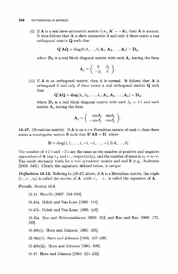
344 FACTORIZATION OF MATRICES
(ii)
(iii)
If A is a real skew-symmetric matrix (i.e., A’ = -A), then A is normal. It then follows that A is skew-symmetric if and only if there exists a real orthogonal matrix Q such that
Q’AQ = diag(O,O,. . . , O , Al, A2,. . . , A t ) = D2,
where D2 is a real block diagonal matrix with each Aj having the form
If A is an orthogonal matrix, then it is normal. It follows that A is orthogonal if and only if there exists a real orthogonal matrix Q such that
Q’AQ = diag(A,, Az, . . . , A,, Al, A2, . . . , A,) = D3,
where D3 is a real block diagonal matrix with each A, = f l and each matrix A, having the form
A, = ( 16.47. (Hermitian matrix) If A is an n x n Hermitian matrix of rank r , then there exists a nonsingular matrix S such that S*AS = D, where
D = d iag ( l , l , . . . ,1, -1, -1,. . . , - 1 , O , O , . . . , O ) .
The number of +l’s and -1’s are the same as the number of positive and negative eigenvalues of A (say r+ and r- , respectively), and the number of zeros is TO = n-r. The result obviously holds for a real symmetric matrix and real S (e.g., Anderson [2003: 6401). Clearly the signature, defined below, is unique.
Definition 16.13. Refering to (16.47) above, if A is a Hermitian matrix, the triple (r+, r- , T O ) is called the inertia of A, while T+ - r- is called the signature of A.
Proofs. Section 16.6.
16.44. Harville [1997: 534-5391.
16.45a. Golub and Van Loan [1996: 4141.
16.45b. Golub and Van Loan [1996: 4161.
16.46a. Rao and Bhimasankaram [2000: 3131 and Rao and Rao [1998: 175, 1901.
16.46b(i). Horn and Johnson [1985: 1051.
16.46b(ii). Horn and Johnson [1985: 107-1081
16.46b(iii). Horn and Johnson [1985: 1081.
16.47. Horn and Johnson [1985: 221-2221.
CONGRUENCE 345
16.7 CONGRUENCE
16.48. (Sylvester’s Law of Inertia) Let A and B be n x n Hermitian matrices. There exists an n x n nonsingular matrix S such that A = SBS’ if and only if A and B have the same inertia (cf. 16.47).
16.49. (Ostrowski) Let A be Hermitian and S nonsingular, both n x n matrices. Then, for each i = 1 , 2 , . . . ,n, there exists a positive real number t9i such that X,,,(SS*) 2 Ot 2 Xmi,(SS*) and
Xi(SAS*) = OiXi(A).
16.50. Let A and B be n x n real or complex symmetric matrices. There exists a nonsingular S such that A = SBS’ if and only if A and B have the same rank.
Proofs. Section 16.7.
16.48-16.50. Horn and Johnson [1985: 223, 224, 2251.
16.8 S I M U LTA N EO US RED U CT I0 N S
16.51. Let A and B be n x n real symmetric matrices.
(a) (i) There exists a real orthogonal matrix Q such that Q’AQ and Q’BQ are both diagonal if and only if AB = BA (that is AB is symmetric).
(ii) The previous result holds for more than two matrices. A set of real symmetric matrices are simultaneously diagonalizable by the same or- thogonal matrix Q if and only if they commute pairwise.
(iii) The above result also holds for Hermitian matrices and unitary Q.
(b) If a real linear combination of A and B is positive definite, then there exists a nonsingular matrix R such that R‘AR and R’BR are diagonal.
(c) If A is also positive definite, there exists a nonsingular S such that S’AS = I, and S’BS = diag(X1, X2,. . . , A n ) , where the X i are the roots of IXA - BI = 0, i.e., are the eigenvalues of A-lB (or BA-’ or A-1/2BA-’/2). The X i are real.
(d) If A and B are both non-negative definite, there exists a nonsingular matrix R such that R‘AR and R’BR are both diagonal.
16.52. Let A and B be n x n complex matrices.
(a) If A and B are both symmetric, there exists a unitary U such that UAU’ and UBU’ are both diagonal if and only if AB is normal; that is, ABBA = BAAB.
(b) If A is Hermitian and B is symmetric, there exists a unitary U such that UAU’ and UBU’ are both diagonal if and only if AB is symmetric; that is AB = BA.
346 FACTORIZATION OF MATRICES
(c) If A is Hermitian positive definite and B is symmetric, then there exists a nonsingular matrix S such that S*AS and S'BS are both diagonal.
(d) Let A be a Hermitian matrix, B be a Hermitian non-negative definite matrix with rank r 5 n, and N be an n x n - r matrix of rank n - r such that N*B = 0. Then:
(i) There exists an n x r matrix L such that L*BL = I, and L*AL = A,
(ii) A necessary and sufficient condition that there exists a nonsingular ma-
where A is an r x r diagonal matrix.
trix R such that R*AR and R*BR are both diagonal is that
rank(N*A) = rank(N*AN).
(iii) A necessary and sufficient condition that there exists a nonsingular ma- trix R such that R*BR and R-'A(R-l)* are both diagonal is
rank(BA) = rank(BAB).
(iv) If, in addition, A is Hermitian non-negative definite, there exists a non- singular matrix R such that R 'AR and R*BR are both diagonal.
(v) If, in addition, A is Hermitian non-negative definite, then there exists a nonsingular matrix R such that R*BR and R-'A(R-l)* are both diagonal.
For other results like (a)-(c) see the table of Horn and Johnson [1985: 2291.
16.53. (Simultaneous Upper-Triangular Reductions) Let A and B be n x n com- plex matrices.
(a) There exist unitary matrices P and Q such that P*AQ = T and P*BQ = S are upper-triangular. If the diagonal elements sii of S are all nonzero, then &(AB-~) = tii/sii for i = 1 , 2 , . . . , n.
(b) If A and B are real, there exist real orthogonal matrices P and Q such that P * A Q is upper quasi-triangular (upper Hessenberg) and P'BQ is upper- triangular.
(c) If A B = B A , then there exists a unitary matrix U such that U*AU and U * B U are both upper-triangular. This result holds for any family of com- muting matrices (Horn and Johnson [1985: 811).
16.54. (Simultaneous Singular Value Decompositions)
(a) (Two Matrices) Let A and B be mxn matrices. There exist unitary matrices P,,, and Qnxn such that A = PElQ ' and B = P&Q*, where Xi ( i = 1,2) are m x n diagonal matrices, if and only if if AB* and B * A are both normal.
(b) (More Than Two Matrices) Given m x n matrices Ai ( i = 1 , 2 , . . . , k ) , there exist unitary matrices P and Q such that A = P&Q* for all i, where the are all diagonal, if and only if each A f A j ( i # j ) is normal and all the pairs of AiAj' (i # j ) commute.
SIMULTANEOUS REDUCTIONS 347
16.55. (Diagonalizable Matrices)
(a) (Two Matrices) Two diagonalizable n x R matrices are simultaneously diag- onalizable; that is, there is a single nonsingular matrix R such that R-’AR and R-’BR are diagonal, if and only if A and B commute (i.e., AB = BA). Commuting matrices play a major role in simultaneous factorizations as we have seen in (16.53~) and (16.54) above. For details see Horn and Johnson [1985: chapter 21.
(b) Let S be an arbitrary (finite or infinite) set of n x n matrices in which every pair commutes. Then:
(i) There is a vector x E Q.” that is an eigenvector of every A E S .
(ii) The members of S can be simultaneously diagonalized.
Proofs. Section 16.8.
16.51a(i). Abadir and Magnus [2005: 1801 and Searle [1982: 312-3131.
16.51a(ii). Rao and Bhimasankaram [2000: 355-3561 and Schott [2005: 163- 1651.
16.48a(iii). Horn and Johnson [1985: 228; they also give other equivalent conditions for the simultaneous diagonalization of two Hermitian matrices] and Rao and Rao [1998: 185-1861.
16.51b. Horn and Johnson [1985: 465, complex case with a real linear com- bination and R* instead of R’] and Schott [2005: 161-162, real case].
16.51~. Abadir and Magnus [2005: 2251 and Searle [1982: 3131. This result also holds for Hermitian matrices (cf. Horn and Johnson [1985: 250-2511 and Rao and Rao [1998: 185-1861),
16.51d. Schott [2005: 1621 and Searle [1982: 313-3141.
16.52a-b. Horn and Johnson [1985: 2351.
16.52~. Horn and Johnson [1985: 4661.
16.52d. For proofs of (d) and further results, see Rao and Mitra [1971: chapter
61.
16.53a. Golub and Van Loan [1996: 3771.
16.5313. Stewart [1972].
16.53~. Zhang [1999: 611 and Meyer [2000a: 522, exercise 7.2.151.
16.54a. Horn and Johnson [1985: 426, exercise 261.
16.5413. Quoted by Rao and Rao [1998: 1921.
16.55a. Horn and Johnson [1985: 501 and Meyer [2000a: 522, exercise 7.2.161.
16.55b. Horn and Johnson [1985: 51-52].
348 FACTORIZATION OF MATRICES
16.9 POLAR DECOMPOSITION
16.56. Let A be an m x n complex matrix of rank r ( r 5 min{m, n})
(a) Suppose m 5 n. Then, using the thin complex version of the singular value decomposition (cf. Section 16.3) we have the polar decomposition
A = PAmQL = (PAmP*)(PQL) = BW,
where B = (AA*)'I2 is an m x m unique Hermitian non-negative definitive matrix of rank r , and W is m x n with orthonormal rows (that is, WW* = Im). If rank A = m, then the matrix W is unique and B is Hermitian positive definite. If A is real. then both B and W can be taken as real.
(b) If m = n, then W is unitary. Furthermore, if A is nonsingular, then W is uniquely determined as B-l A.
(c) Let m 2 n. By applying (a) to A* we can write A = VC, where the m x n matrix V has orthonormal columns and C is an n x n unique non-negative definite Hermitian matrix of rank r . If A nonsingular, then V = W.
(d) B = C if and only if A is normal.
16.57. Suppose that the n x n matrix A has a polar decomposition A = BW. Then it follows from (16.56d) above that A is normal if and only if BW = WB.
Proofs. Section 16.9.
16.56. Horn and Johnson [1985: 412-4141.
16.57. Abadir and Magnus [2005: 226, real case] and Horn and Johnson [1985: 4141.
16.10 MISCELLANEOUS FACTORIZATIONS
16.58. (Takagi Factorization) Let A = ( a z j ) be a real or complex symmetric n x n matrix. Then A can be expressed in the form A = QDQ' (note Q' and not Q"), where Q is an n x n unitary matrix and D is a real non-negative diagonal matrix. The columns of Q are an orthogonal set of right eigenvectors of AA, and the corresponding diagonal elements of D are the non-negative square roots of the corresponding eigenvalues of AA.
16.59. Any square matrix A can be factorized as A = SQDQ'S-l, where S is nonsingular, Q is unitary, and D is diagonal with non-negative main diagonal entries; all matrices are n x n.
16.60. For any square matrix A, there exists a unitary Q and upper-triangular matrix V such that A = QVQ', where all matrices are n x n, if and only if the eigenvalues of AA are real and non-negative. When this condition is true, the main diagonal elements of V may be chosen to be non-negative.
MISCELLANEOUS FACTORIZATIONS 349
16.61. If H is Hermitian, there exists a unitary marix Q such that Q*AQ is tridiagonal (and also Hermitian).
16.62. (Upper Hessenberg Reduction) unitary matrix Q such that QAQ* is upper Hessenberg.
Proofs. Section 16.10.
For any square matrix A there exists a
16.58. Horn and Johnson [1985: 157, 2041 and quoted by Rao and Rao [1998: 1921.
16.59. Horn and Johnson [1985: 157, 2101.
16.60. Quoted by Rao and Rao [1998: 1921.
16.61. Quoted by Rao and Rao [1998: 1901. The real case (Jacobi’s reduction) is discussed by Meyer [2000a: 3531.
16.62. Quoted by Rao and Rao [1998: 1901. It is also described by Meyer [2000a: 351, real case].

This Page Intentionally Left Blank
CHAPTER 17
D I F F E R E N T I AT I0 N
Methods of differentiation and differentials involving scalars, vectors, and matrices are used extensively in statistics. Applications include maximum likelihood and least squares estimation, large sample theory, statistical computing, and Jacobians, the subject of the next chapter. Turkington [2002], for example, applies first and second order differentiation to find maximum likelihood estimates and variance estimates for linear regression models, autoregressive time series, seemingly unre- lated regression equations, and linear simultaneous equations models. Magnus and Neudecker [ 19991 do a similar thing with multivariate models, errors-in-variables models, nonlinear regression, and simultaneous equation models.
Differentiation is also used in sensitivity analysis and perturbation methods, which endeavor to determine the perturbation in a system when there are small changes in the parameters. It is also used in the derivation of elasticities (a term from economics), where one determines the proportional perturbation when there is a proportional change in a parameter. Some examples are model fittting (e.g., Seber and Wild [1989: 121-126, 668]), ecolological population dynamics (Caswell [2001, 2007]), and multivariate elliptical linear regression models (Liu [2002b]). The chapter closes with a few results on difference equations.
17.1 INTRODUCTION
I have endeavored to categorize the methods of differentation for easy reference, though some results, especially relating to a function of a function, fit into more than
A Matrix Handbook for Statisticians. By George A. F. Seber Copyright @ 2008 John Wiley & Sons, Inc.
351
352 DIFFERENTIATION
one category. There is also some overlap of topics as one can consider differentiation either with respect to a vector or matrix, or with respect to an element of a vector or a matrix. A helpful survey of the subject including an historical overview is given by Nel [1980]. He also considers differentiation with respect to patterned matrices (cf. Section 18.3.5).
17.2 SCALAR D I F F E R E NT I AT I0 N
For some analytical background to the subject in a statistical context, the reader is referred to Abadir and Magnus [2005: chapter 131, Magnus and Neudecker [1999], and Schott [2005: chapter 91.
17.2.1
Definition 17.1. We first define the derivative of a matrix or vector with respect to a scalar. If A(t) = ( q ( t ) ) , then aA(t)/at is defined to be (aaij(t)/at); that is, the derivative of A(t) is obtained by differentiating each element of A. The same is true for a vector a(t) = (ai(t)).
Unless specified (e.g., A is symmetric), we assume that the elements of all the matrices differentiated are functionally independent (i.e., unconstrained). Also, the following apply when we have a vector t = ( t t , t z , . . . , t,.)’ and at is replaced by ati.
17.1. We have from the definition:
Differentiation with Respect to t
17.2. (Products) Noting that 8 is the Kronecker product, the following result is used extensively in the next section.
d(A(t) 8 B(t)) aA dB = - @ B + A A - .
at at at (b)
17.3. (Inverse)
(a) Differentiating AA-l = I for nonsingular A(t), we get
(b) If R does not depend on t, then differentiating [R’A(t)R]-lR’A(t)R = I gives us
SCALAR DIFFERENTIATION 353
(c) If A is symmetric and B(t) = R[R’A(t)R]-lR’, where R does not depend on t, then, using (b), we obtain
dA - = -B-B. aB a t a t
(d) If A-(t) is a weak inverse of A(t), then differentiating
a A a t a t
A 1 -AA--A-A. A- aA-(t)
Further details are given in (17.8) below.
A’ = -A(A’A)- ’(AA’) (A’A1-A’. a t (el A at
17.4. (Determinants) If A(t) is nonsingular, then
8 log(det A) a t
AA-A = A g’ 1ves us
The result is also true if A is symmetric. A further result follows by noting that
a d e t A dlog(det A) at ’
= det A at
a[trace(A(t)] = trace [ 8“) at
17.5. (Trace)
deAt a t - = AeAt. 17.6. (Exponential)
Proofs. Section 17.2.1.
17.2. Graham [1981: 381.
17.3d-e. Searle [ 1982: 3351.
17.4. Searle [1982: 337-3381.
17.6. Abadir and Magnus [2005: 3681.
17.2.2
We now consider the special case when t is an element of an n x 1 vector x = (xt). The results in this section still apply if F is a matrix function of a matrix X = ( x z J ) , and we replace x, by xz3 .
17.7. Let F be a square matrix function of a vector x = (xl,x2,. . . , xn)’, then from (17.4) and (17.3a) we have the following.
Differentiation with Respect to a Vector Element
d trace [ F (x) ] ax, = trace (g)
354 DIFFERENTIATION
(b) Suppose F is nonsingular.
d det [F( x)]
dlogdet[F(x)] 1 d d e t F 8x2 d e t F axi
dF dF-1 8x2 d X i
d X i
axi -- - -
- - - -F-l-F-l.
dlogdet(AF-lB) = -trace
If adjF is the adjoint matrix of F, then adjF = (det F)F-' and
dadjF d d e t F dF-1
dxa dxa 8x1 F-' + det F-. -
~~ -
(c) (Kronecker Product) Let F and G be p x q and T x s matrix functions of x.
(i)
(ii)
17.8. Let
dG dF = F @ - + -@G.
d ( F @ G) aXi axc, dxa
We can replace F by vecF and G by vecG in the above equation.
dvec (F @ G) dXi
where K,, (=
d(vec F @ vec G) = (1, @ K P @ I T ) 7
is the commutation matrix.
F be a p x q matrix function of x. If F- is a weak inverse of F, then, un- der certain analytical conditions including continuous differentiability and constant rank in some neighborhood, we have
dF- dF dXi 8x2
F-F = -FF--F-F.
dG dF 8x2 8x2
In particular, there exists a weak inverse G of F such that - = -G-G.
17.9. Let F be a p x q matrix function of x. If F+ is the Moore-Penrose inverse of F, then, under certain analytical conditions including continuous differentiability and constant rank in some neighborhood, we obtain
- ~ - dF+ dXi
17.10. (Eigenvalue and Eigenvector) Let F be a symmetric matrix function of an n x 1 vector x. Let X be a simple eigenvalue of F (i.e., one with an algebraic multiplicity of 1) and corresponding right eigenvector u of unit length. Then, given Fu = X u and H+, the Moore-Penrose inverse of H = F - X I , we obtain
SCALAR DIFFERENTIATION 355
17.11. Consider the idempotent matrix P = X(X’WX)-X‘W, where X is n x p and W is an n x n positive definite matrix such that the elements of W and/or X are functions of a vector z. Then, under certain analytical conditions including continuous differentiability and constant rank in some neighborhood, we obtain
ax ax - = (I, - P)-(X’WX)-X’W + x(x’wx)- ( - ) ’w(In - P) aP az, azi azi
dW
82, +x(x’wx)-x’-(I , - P).
17.12. Suppose X = X(4), where X is n x p of rank p and is a function of 4 = (41, 4 2 , ‘ ’ ’ , M’. Then,
adet(X’X) = det(X‘X) trace a4i
where X+ is the Moore-Penrose inverse of X. This theory arises in nonlinear modeling.
Proofs. Section 17.2.2.
17.7. Harville [1997: 305, 307-3081 and Harville [2001: 158, exercise 321
17.8. Harville [1997: 3121.
17.9. Harville [1997: 5111.
17.10. Harville [1997: section 21.15 for proofs and analytical background].
17.11. Harville [1997: 3151. Derivatives are also given for WP and W - WP.
17.12. Bates and Watts [1987] and Bates and Watts [1988: chapter 41 give further details. For a summary see Seber and Wild [1989: 543-5441.
17.2.3
Definition 17.2. We define the matrix E,, to be an m x n matrix with 1 in the i , j t h position and zeros elsewhere. Thus E,, = ez,mek,3, where ez,m is the i th column of I, and e3,, is the j t h column of I,.
In what follows, we consider the special case of t = x,,, an element of the real mxn matrix X, and include differentiation with respect to a vector element. Results in this section can be derived using the properties given in the previous section along with (17.13) below. We assume that the elements of X are functionally independent (i.e., are “unconstrained’), unless stated otherwise. When m = n, then E,, = E;,.
Differentiation with Respect to a Matrix Element
17.13. (Basic Result)
(a) It is straightforward to show that
ax Eij 1 X unconstrained, E,j + Elj - bijEii, X symmetric,
where bij = 1 when i = j and 6ij = 0 when i # j .
356 DIFFERENTIATION
ax’ (b) dzij = (G) (c) To convert a result given below about an unconstrained X into one for sym-
metric X, we simply replace E,, by E,, + E:, - SZ3EZZ.
17.14. (Products) We assume that the following matrices are conformable and X is unconstrained. The results follow directly from (17.1) and (17.2). Further results can be obtained by setting A and/or B equal to the identity matrix.
~ ( A X B ) ax axij 8 X i j
= A-B = AEijB.
a(AXB) = E:, AXB + X’AE,, B. ~(X’AXB) ax’
= -AXB + X’ (‘) ax,, ax,, ax,,
(d) a(xAx’B) = E,j AX’B + XAE:, B. axzj
= AEB = AE,,X’B + AXE:,B. a(AXX’B)
ax,, ax,,
( f ) a(XAXB) = EijAXB + XAEijB. axij
= EijX’X + XE:,X + XX’Eij. axx‘ x
(h) ~ axij 17.15. (Inverses)
(a) If BXC is nonsingular, we differentiate (BXC)(BXC)-’ = I to get (cf. 17.3a)
a{A(BXC)-lD) = -A(BXC)-lBEijC(BXC)-lD. axij (b) Suppose X is m x m and nonsingular. From (a) we have
where y, is the i th column and zi is the j t h row of X-l.
If X is symmetric, then using (17.13~) we have
ax-1 if i = j ,
where y, is the i th column of X-l.
SCALAR DIFFERENTIATION 357
17.16. (Determinants) Suppose X is square and Ez3 is the cofactor of x , ~ . Then
-= { d det X E 2 3 , X unconstrained, ax23 (2 - & ) E 2 3 , x = X',
where 6,) = 1 when i = j and 0 otherwise.
17.17. (Powers) Let X be nonsingular, and let Ic be a positive integer.
(a) We can prove by induction that
for Ic = 1 , 2 , . . ., where Xo = I,.
(b) Differentiating XkXPk = I gives us
17.18. (Some Matrix Functions) where X is unconstrained.
Let Y be a nonsingular matrix function of X,
= (detY) trace Y-'- [ d d e t Y
When X is symmetric we can use (17.13~) in the following applications.
(i) If Y = AXB, then (from 17.14a)
ddet(AXB) = det(AXB) t r a ~ e [ ( A x B ) - ~ A E , j B ] axij
= det (AXB) { [B(AXB) -'A]'}ij.
(ii) If Y = X'AX, then (from 17.14~)
= det(X'AX) trace{ (X'AX)-' [EljAX + X'AEij]}. d det(X'AX)
d X i j
dvec Y dY = vec -.
(b) dzij l3Xij
d trace Y (c) d X , j = trace (e) .
We can get a corresponding result for (Y-')' by simply replacing Y by Y', as (Y-')' = (Y')-'.
358 DIFFERENTIATION
17.19. (Eigenvalue and Eigenvector) Let X be a symmetric n x n matrix with simple eigenvalue X (i.e., has an algebraic multiplicity of l), and corresponding eigenvector u = (ui) of unit length. Then
2 2 - = 2uu‘ - diag(u,,u2, . . . ,u:). ax
d X i j
Also, if gj is the j t h column of H+, the Moore-Penrose inverse of H = X - XI,, we have - = { au -uigi , if j = i,
8 X i j - (u jg i + u i g j ) , if j < i.
Proofs. Section 17.2.3.
17.14. Graham [1981: 60-64, 691.
17.15b. Harville [2001: 130, exercise 211.
17.16. Searle [1982: 3361.
17.17. Graham [1981: 67-68].
17.18. Harville [1997: section 15.81.
17.19. Harville [1997: 5671.
17.3 VECTOR D I F FE R EN TI AT I 0 N : SCALAR F U N C T I0 N
17.3.1 Basic Results
Definition 17.3. I f f is a function of x, we denote the vector of partial derivatives
(a f /ax i ) by the column vector a f /ax, that is, - =
row vector a f /ax’ = (a f /ax)’. Some authors (e.g., Dhrymes [2000]) reverse the notation.
17.20. (Basic Results) Let x and a be n x 1 vectors, and let A an n x n matrix.
af (g). We also define the
8x‘Ax (b) dx - - (A + A’)x, or 2Ax if A is symmetric.
17.21. (Chain Rule) If z is a differentiable scalar function of y, and y is a differ- entiable function of x, then
which can be expressed in the form of the row vector
a z a z ay ax, dy’ ax,‘
- - - - . -
VECTOR DIFFERENTIATION SCALAR FUNCTION 359
In terms of column vectors,
The function z might include functions such as the trace, the determinant, and quadratic expressions.
Proofs. Section 17.3.1.
17.20. Abadir and Magnus [2005: 356, transposed].
17.3.2 x = vec X
In applying the following results using the chain rule above, it can be more con- venient to work with d(vecX)’ instead of dvecX. The right-hand side is then transposed, as indicated in (17.22) below. Some authors use the reverse notation (e.g., Dhrymes [2000]). Note that the following derivatives are all column vectors.
17.22. If f ( X ) is a scalar function of the matrix X, then
17.23. (Trace)
d trace(AXB) = vec ( A’B’) .
vec x We can obtain this result directly by noting that
trace(AXB) = trace(BAX) = vec (A’B’)’vec X,
and using (17.20a). We can set A or B equal to I.
= [(B’ @ A ) + (B @ A’)]vecX. d trace(X’AXB)
(b) vec x Provided that the appropriate matrices are square, other results follow from trace(CD) = trace(DC) and trace C = trace C’. For example,
trace(X’AXB) = trace(AXBX’) = trace(XBX’A) = trace(BX’AX).
17.24. (Determinants and Log Determinants) are nonsingular, and we use the result vec (AXB) = (B’ @ A)vec X.
The following matrices X and Y
ddet d vec X
= vec [(adjX)’] = (det X)vec (X-”).
If Y = X‘AX, then
= det Y [(Y-” @ A ) + (Y-’ @ A’)]vec X. d d e t Y dvec X
360 DIFFERENTIATION
When A is symmetric, then Y is also symmetric and
d d e t Y d vec X
= 2detY[(Y-’ @A)vecX.
(c) If Y = XBX’, then
d d e t Y d vec X
= det Y[B @ (Y-’)’ + (B’ @ Y-’)]vecX.
When B is symmetric, then Y is symmetric and
d d e t Y d vec X
= 2 det Y [B @ (Y-l)]vec X.
(d) If Y is one of the above functions, then
d(1ogdet Y) 1 d d e t Y ~~
- - a vec X det Y avec X ’
Proofs. Section 17.3.2.
17.23. Dhrymes [2000: 156-157, transposed] and Rogers [1980: 541.
17.24a. Rao and Rao [1998: 2291 and Schott [2005: 3601.
17.24b. Abadir and Magnus [2005: 372-373, transposed].
17.24a-d. Turkington [2002: chapter 41,
17.3.3 Function of a Function
17.25. Suppose y = w‘Az, where A is m x n and w, z, and A are all functions of x. We wish to find the row vector dyldx‘. We first note from (11.16b) and (11.15~) that
y = vec y = (z’ @ w’)vec A = (z @ w)’vec A = [vec (wz’)]’vec A.
Then using W‘AZ = z’A‘w, we get
dW I ,dvecA az = z’A’- + [vec (wz ) I ~ + w‘A-
ax’ dX’ ax’ dX’
dy
17.26. Let y = trace[F(Z)], where F is a square matrix function of Z and Z is a function of x. Then, by the chain rule (17.21), we obtain
dy dvecZ dy- - .~ ax’ a(vecZ)’ ax’ ’
where dy/d(vecZ)’ can be obtained from (17.23) and transposing. We give three examples from Dhrymes [2000: section 5.41.
d trace(AZB) d vec Z = vec ( A’,’ )’ - .
(a) Ox’ 8x1
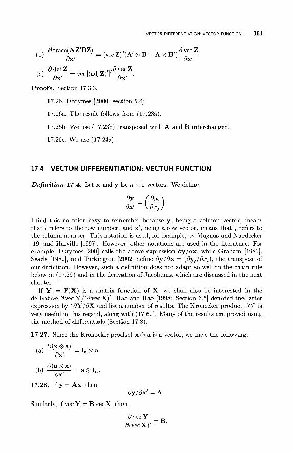
VECTOR DIFFERENTIATION: VECTOR FUNCTION 361
a trace( AZ’BZ) a vec Z dX/ ax’ .
= (vecZ)’(A’@B+A@B’)- (b)
ddet Z dvec Z = vec [(adjZ)’]’-
(c) dx’ .
Proofs. Section 17.3.3.
17.26. Dhrymes [2000: section 5.41.
17.26a. The result follows from (17.23a).
17.26b. We use (17.2313) transposed with A and B interchanged.
17.26~. We use (17.24a).
17.4 V ECTO R D I F F E R E NT I AT I0 N : VECTO R F U N C T I0 N
Definition 17.4. Let x and y be n x 1 vectors. We define
-=($>- a Y ax’
I find this notation easy to remember because y, being a column vector, means that i refers to the row number, and x‘, being a row vector, means that j refers to the column number. This notation is used, for example, by Magnus and Nuedecker [19] and Harville [1997]. However, other notations are used in the literature. For example, Dhrymes [200] calls the above expression dy/dx, while Graham [1981], Searle [1982], and Turkington [2002] define dy/dx = (dyj/azi), the transpose of our definition. However, such a definition does not adapt so well t o the chain rule below in (17.29) and in the derivation of Jacobians, which are discussed in the next chapter.
If Y = F(X) is a matrix function of X , we shall also be interested in the derivative dvecY/(dvecX)’. Rao and Rao [1998: Section 6.51 denoted the latter expression by *dY/dX and list a number of results. The Kronecker product “@” is very useful in this regard, along with (17.60). Many of the results are proved using the method of differentials (Section 17.8).
17.27. Since the Kronecker product x 8 a is a vector, we have the following.
a(x 8 a) (a) ax, = I, @a.
- a@.,. d(a 8 x)
(b) dx’ - 17.28. If y = Ax, then
ay/ax’ = A.
Similarly, if vec Y = B vec X , then
d vec Y d(vec X)’
= B.
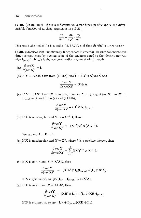
362 DIFFERENTIATION
17.29. (Chain Rule) If z is a differentiable vector function of y and y is a differ- entiable function of x, then, arguing as in (17.21),
az dz d y dx’ dy’ dx”
- - -
This result also holds if z is a scalar (cf. 17.21), and then dz/dx’ is a row vector.
17.30. (Matrices with Functionally Independent Elements) In what follows we can obtain special cases by putting some of the matrices equal to the identity matrix. Also I(,,,) (= K,,) is the vec-permutation (commutation) matrix.
(b) If Y = A X B , then from (11.16b), vecY = (B’ 8 A)vecX and
d vec Y d(vec X)’
= B’@A.
(c) If Y = AX’B and X is m x n, then vec Y = (B’ 8 A)vec X’, vec X’ = I(,,,)vecX and, from (a) and (11.16b),
d vec Y d(vec X)’ = (B’ @ A P ( n , m )
(d) If X is nonsingular and Y = AX-lB , then
vec Y = -(X-’B)’ @ (AX-’)
d(vec X)’
We can set A = B = I.
(e) If X is nonsingular and Y = X k , where k is a positive integer, then
k
= C((X’)”-i @ xi-1). d vec Y
d(vec X)‘ i = l
( f ) If X is m x n and Y = X’AX, then
d vec Y d(vec X)‘ = (X’A’ 8 L)I(,,,~ + (I, 8 X’A).
If A is symmetric, we get ( I n 2 + I(,,,))(I, 8 X’A).
(g) If X is m x n and Y = XBX’, then
If B is symmetric, we get (1,~ + I(,,,))(XB @ Im).
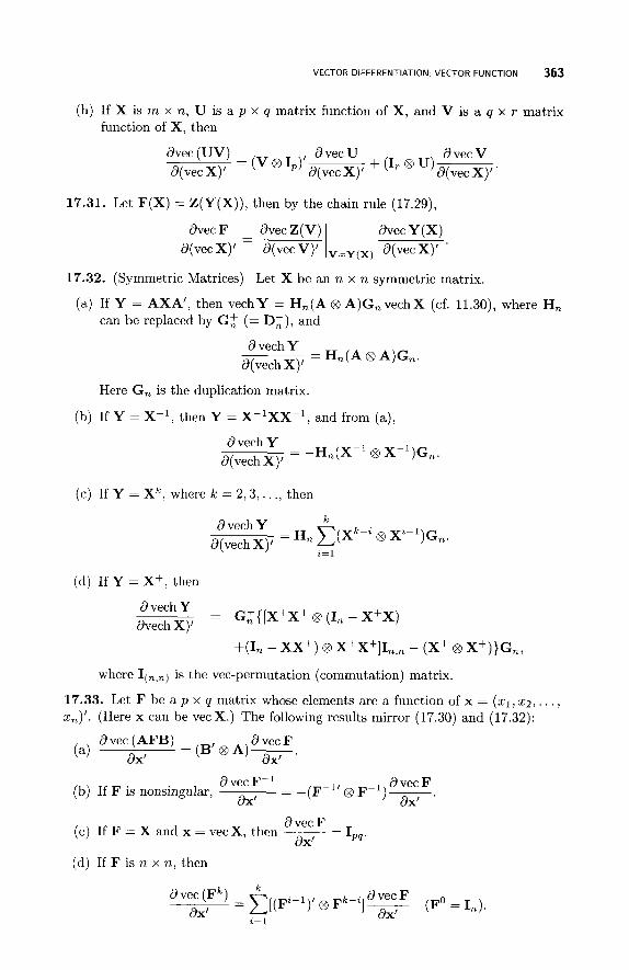
VECTOR DIFFERENTIATION VECTOR FUNCTION
(h) If X is m x n, U is a p x q matrix function of X, and V is a q x T
function of X, then
363
matrix
17.31. Let F(X) = Z(Y(X)), then by the chain rule (17.29),
dvec F dvec Y (X) v,y(x) d(vec X)' '
17.32. (Symmetric Matrices) Let X be an n x n symmetric matrix.
(a) If Y = AXA', then vechY = H,(A @ A)G,vechX (cf. 11.30), where H, can be replaced by G: (= D:), and
13 vech Y d(vech X)l
= H,(A 8 A)G,.
Here G, is the duplication matrix.
(b) If Y = X-', then Y = X-lXX-l, and from (a);
d vech Y d(vech X)' = -H,(X-' @ X-')G,.
(c) If Y = Xk, where k = 2 , 3 , . . ., then
k d vech Y d(vech X)'
= H, x ( X k p i @ Xi-')G, i= l
(d) If Y = X+, then
d vech Y dvech X)'
= G,f{ [X+X+ @ (I, - X + X )
where I(,,,) is the vec-permutation (commutation) matrix.
17.33. Let F be a p x q matrix whose elements are a function of x = (XI, ~ 2 , . . . , (Here x can be vec X.) The following results mirror (17.30) and (17.32):
8 vec (AFB) d vec F = (B' @ A)-.
ax' 8x1
d vec F-l = -(F-l' @ F-l)-. d vec F ax' 8x1
If F is nonsingular,
d vec F dX'
If F = X and x = vecX, then - - - I P T
If F is n x n, then
k dvec (Fk) d vec F
= C[(F"-')' @ Fk-Zldx, (Fo = I,). i= 1
dX'
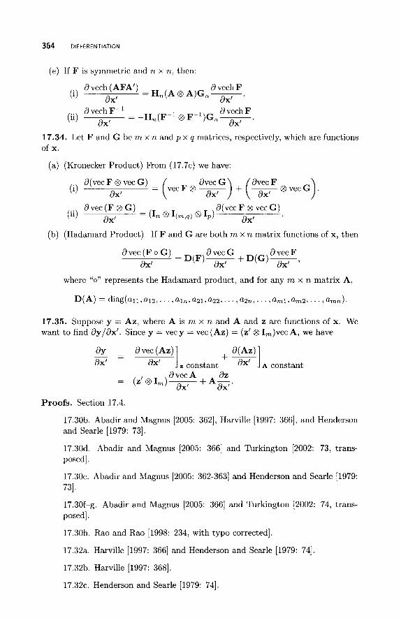
364 DIFFERENTIATION
(e) If F is symmetric and n x n, then:
d vech ( AFA’) d vech F = H,(A @ A)G,-.
( 4 Ox’ dX’ d vech F-’ d vech F
(ii) = -H,(F-~ @ F-~)G,- dX’ dX’
17.34. Let F and G be m x n and p x q matrices, respectively, which are functions of x.
(a) (Kronecker Product) From (17.7~) we have:
a( vec F @ vec G ) = ( r e c F @ w ) + (-8vecG dvec F dX’ dX’ dX’ (4
dvec (F 8 G) -
(b) (Hadamard Product) If F and G are both m x n matrix functions of x, then
d(vec F 8 vec G) dX’ (ii) - (In 63 b , q ) 8 I P ) dX’
dvec (F o G) d vec G dvec F dX’ 1 D(F)- dX’ + D ( G ) T ’
where “0” represents the Hadamard product, and for any m x n matrix A,
D(A) =diag(uii,aiz,...,ai,,azl,azz,...,azn,.. .,aml,ama,. . . ,amn)
17.35. Suppose y = Az, where A is m x n and A and z are functions of x. We want to find dy/dx’. Since y = vecy = vec (Az) = (z’ 8 1,)vec A, we have
d y - d vec ( Az) dX’
-
dvecA dz dX’ dX‘
= (z’81m)- + A -
Proofs. Section 17.4.
17.30b. Abadir and Magnus [2005: 3621, Harville [1997: 3661, and Henderson and Searle [1979: 731.
17.30d. Abadir and Magnus [2005: 3661 and Turkington [2002: 73, trans- posed].
17.30e. Abadir and Magnus [2005: 362-3631 and Henderson and Searle [1979: 731.
17.3Of-g. Abadir and Magnus [2005: 3661 and Turkington [2002: 74, trans- posed].
17.30h. Rao and Rao [1998: 234, with typo corrected].
17.32a. Harville [1997: 3661 and Henderson and Searle [1979: 741.
17.32b. Harville [1997: 3681.
17.32~. Henderson and Searle [1979: 741.
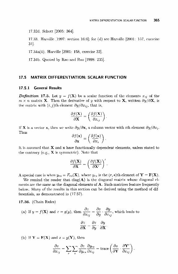
MATRIX DIFFERENTIATION: SCALAR FUNCTION 365
17.32d. Schott [2005: 3641.
17.33. Harville [1997: section 16.61; for (d) see Harville [2001: 157, exercise 311.
17.34a(ii). Harville [2001: 158, exercise 321.
17.34b. Quoted by Rao and Rao [1998: 2351.
17.5 MATRIX DIFFERENTIATION: SCALAR FUNCTION
17.5.1 General Results
Definition 17.5. Let y = f(X) be a scalar function of the elements z , ~ of the rn x n matrix X. Then the derivative of y with respect to X, written ay/aX, is the matrix with (i, j ) t h element ay/dx,, , that is,
If X is a vector x, then we write ay/dx, a column vector with i th element dy/azi. Thus
It is assumed that X and x have functionally dependent elements, unless stated to the contrary (e.g., X is symmetric). Note that
A special case is when yrs = F,,(X), where yrs is the (T , s) th element of Y = F(X). We remind the reader that diag(A) is the diagonal matrix whose diagonal el-
ments are the same as the diagonal elements of A. Such matrices feature frequently below. Many of the results in this section can be derived using the method of dif- ferentials, as demonstrated in (17.57).
17.36. (Chain Rules)
az az ay axij ay axij (a) If y = f (X) and z = g(y), then ~ = - . -, which leads to
az az ay ax ay ax’
-
(b) If Y = F(X) and z = g(Y), then
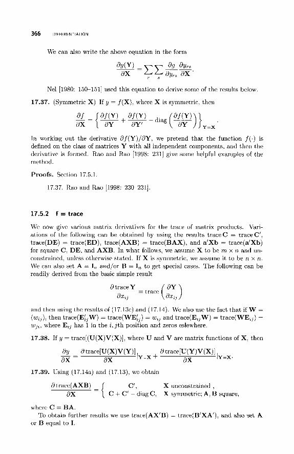
366 DIFFERENTIATION
We can also write the above equation in the form
Nel [1980: 150-1511 used this equation to derive some of the results below.
17.37. (Symmetric X) If y = f(X), where X is symmetric, then
In working out the derivative df(Y)/aY, we pretend that the function f ( . ) is defined on the class of matrices Y with all independent components, and then the derivative is formed. Rao and Rao [1998: 2311 give some helpful examples of the method.
Proofs. Section 17.5.1.
17.37. Rao and Rao [1998: 230-2311.
17.5.2 f = trace
We now give various matrix derivatives for the trace of matrix products. Vari- ations of the following can be obtained by using the results trace C = trace C’, trace(DE) = trace(ED), trace(AXB) = trace(BAX), and a’Xb = trace(a’Xb) for square C , DE, and A X B . In what follows, we assume X to be m x n and un- constrained, unless otherwise stated. If X is symmetric, we assume it to be n x n. We can also set A = I, and/or B = I, to get special cases. The following can be readily derived from the basic simple result
d trace Y = trace (g)
ax,,
and then using the results of (17.13~) and (17.14). We also use the fact that if W = (wzJ) , then trace(E:,W) = trace(WE’ ) = wzJ and trace(E,,W) = trace(WE,,) = wJz, where E,, has 1 in the i , j t h position and zeros eslewhere.
17.38. If y = trace[(U(X)V(X)], where U and V are matrix functions of X, then
dy - d trace[U(X)V(Y)] d X dX
d trace[U(Y)V (X)] dX
~ IY=X. IY=X +
17.39. Using (17.14a) and (17.13), we obtain
d trace(AXB) C‘ , X unconstrained , d X
where C = BA.
or B equal to I.
= { C + C’ - diag C , X symmetric; A, B square,
To obtain further results we use trace(AX’B) = trace(B’XA’), and also set A
MATRIX DIFFERENTIATION SCALAR FUNCTION 367
17.40. If A is m x m, B is n x n, and X is unconstrained, we have from (17.14~) that a trace(X'AXB) a trace(XBX'A)
= A X B + A'XB'.
An important special case is when B = I, and A is symmetric. Then
- - ax ax
d trace( X' AX) = 2AX. ax
17.41. Using (17.14f) and (17.13), we obtain
d trace(XAXB) H'l X unconstrained , d X = { H + H' - diag H, X symmetric,
where H = B X A + AXB. We can get the special case of t r a ~ e [ ( A X ) ~ ] by noting that t r a ~ e [ ( A X ) ~ ] = trace(AXAX) = trace(XAXA). Also, we can set B = I.
17.42. If X is nonsingular and unconstrained, we have from (17.15a):
- - a trace(AX-'B)
ax (b) From (a) we have - (x- 'BAX- l )'.
- - - d trace X-l
ax ( c ) A useful special case is -(X-2)'
(d) When X is symmetric, we have from (17.13) that
d trace X-l = -2(X-2) + diag(X-2). ax
17.43. Using (17.17a) and (17.13), we have for k = 2,3, . . .
d trace Xk k(X"-l)', X unconstrained, ax = { 2kX"-' - k diag(Xk-'), X symmetric.
17.44. Suppose X is unconstrained.
8 trace ex = (ex)'
(a) ax
Proofs. Section 17.5.2.
17.38. Rao and Rao [1998: 2321.
17.39. Harville [2001: 116, exercise 81.
17.40. Graham [1981: 77-78].
17.44a. Abadir and Magnus [2005: 368, exercise 13.291.
17.44b. The derivative is etrace(x2)d trace(X2)/aX, and then use (17.14f) with A = B = I.
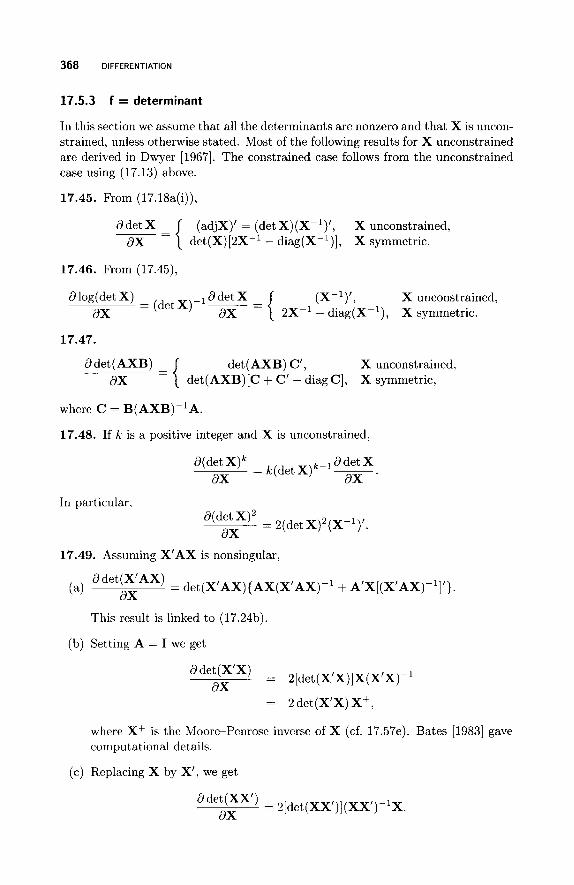
368 DIFFERENTIATION
17.5.3 f = determinant
In this section we assume that all the determinants are nonzero and that X is uncon- strained, unless otherwise stated. Most of the following results for X unconstrained are derived in Dwyer [1967]. The constrained case follows from the unconstrained case using (17.13) above.
17.45. From (17.18a(i)),
d d e t X (adjx)’ = (det X)(X-’)’, X unconstrained, ax det(X)[2XP1 - diag(X-I)], X symmetric.
17.46. From (17.45),
dlog(det X) d d e t X (X-l)’, X unconstrained, = { 2X-’ - diag(X-’), X symmetric.
= (det X)-’- d X dX
17.47.
d det (AXB) det(AXB) C’, X unconstrained, d X { det(AXB)[C + C’ - diag C ] , X symmetric,
where C = B(AXB)-’A.
17.48. If k is a positive integer and X is unconstrained,
d d e t X = k(det X ) ” - ’ ~
dX dX . d(det X)k
In particular,
= 2(det X)’(X-l)’. d(det X)’
dX
17.49. Assuming X’AX is nonsingular,
ddet(X’AX) = det(X’AX){AX(X’AX)-’ + A’X[(X’AX)-’]’}. (a) ax
This result is linked to (17.2413).
(b) Setting A = I we get
= 2 [det (X’X)] X(X’X) - ’ ddet(X’X) d X
= 2 det(X’X) X’,
where X+ is the Moore-Penrose inverse of X (cf. 17.57e). Bates [1983] gave computational details.
(c) Replacing X by X’, we get
a det(XX’) = 2[det (XX’)] (XX’)-’ X. dX
MATRIX DIFFERENTIATION: SCALAR FUNCTION 369
17.50. Let F(X) be a square nonsingular matrix function of X, and let G ( X ) = C[F(X)]-’A. Then
det[F(X)](GXB + G’XB’), if F(X) = AXBX’C, adet[(F(X)I = { det[F(X)](BXG + B’XG’), if F(X) = AX’BXC,
det[F(X)](GXB + BXG)’, if F(X) = AXBXC. ax
17.51. If X is nonsingular,
8 det (AX-‘ B) - det(AX-’B)C’, X unconstrained, dX = { -det(AX-’B)[C + C’ - diag C], X symmetric,
where C = [X-lB(AX-lB)- lAX-l] .
17.52. If F is a nonsingular matrix function of X with det F > 0, then
a log det F a d e t F = (det F ) - ’ ~ ax ax ’
This can be applied to all the previous results.
Proofs. Section 17.5.3.
17.45. Mathai [1997: 91 and Searle [1982: 3371; see also (17.5713).
17.46. Henderson and Searle [1979: 761 and Searle [1982: 331; see also (17.57d).
17.47. Rogers [1980: 521; see also (17.57d).
17.48. Graham [1981: 75-76] and Magnus and Neudecker [1999: 179, k = 21.
17.49a. This result also follows from (17.50).
17.4913. Magnus and Neudecker [1999: 1791 and Rogers [1980: 521.
17.49~. Magnus and Neudecker [1999: 1791.
17.50. Quoted by Magnus and Neudecker [1999: 1801.
17.51. Rogers [1980: 521.
17.5.4 f = yrs
17.53. In what follows we assume that X and Eij (with 1 in the ( i , j ) t h position and zeros elsewhere) are both m x n matrices.
370 DIFFERENTIATION
= AXE:, + A‘XE,,. W’AX) , , (d) ax
(e) ax
( f ) ax
= E,,X’A’ + A’X’E,, .
= AX’E;, + E;,x’A’. a( X’AX’),,
k- 1
(g) If k is a positive integer, ~ = E(X’)jE,s(X’)n-j-l, where j = O
ax xo = I.
Proofs. Section 17.5.4.
17.53. Graham [1981: 60-681.
17.5.5 f = eigenvalue
17.54. If X is a nonrepeated (simple) eigenvalue of the square matrix X with left eigenvector v and right eigenvector u. then
(a)
- = v(v’u)-lu’ dX dX
(b) If A, is a simple eigenvalue, eigenvector (i.e., Ub.0 = I) ,
X is symmetric, and Ug is the normalized right which is also the left eigenvalue, then
Proofs. Section 17.5.5.
17.54a. Lancaster [1964] and Nel [1980: 1411.
17.5413. Lancaster [1964] and Magnus and Neudecker [1999: 1801.
17.6 TRANSFORMATION RULES
We now give some transformation rules that enable us to use the results from one type of differentiation to obtain results for other types.
17.55. Let X be an m x n matrix, and let Y be a function of X. The following equivalent expressions (adapted from Graham’s [ 1981: 65, 741 two “transformation principles”) apply for all conformable At, Bt, C,, and D,, including functions of X, and are simply different ways of writing ayrs/dx,,. If we obtain an expression like (1) or (2) below, for example, in the process of differentiation, then we can immediately obtain (3), which may be more difficult t o get directly.
MATRIX DIFFERENTIATION. MATRIX FUNCTION 371
It should be noted that E,, and E,, may be of different sizes. We also recall (cf. 11.19a) that if C and D are both m x R , then
I (m,n) (D €3 C’) = (C’ €3 D)I(n,m).
17.7 MATRIX DIFFERENT I AT1 0 N : MATRIX F U N C T I0 N
Definition 17.6. Let Y = F(X), where Y is p x q and X is m x n. Then the derivative of Y with respect to X can be defined in different ways. One method is to use the mp x nq matrix (MacRae [1974] and Rogers [1980])
k 3 2 2 . . . d ax ax
d Y dX . . . . .
where the multiplication of a matrix element by a derivative operator corresponds to the operation of differentiation. Some authors-for example, Vetter [1970] - have used the reverse order (d/dX) BY in the above definition. Rogers defines the latter to be a y a y
a y a y aXz1 aXz2
- ~ . . . ~
ax11 az12
- - ... - . . .
This is the definition for dY/dX used by Graham [1981: chapter 61. The above definitions can also be used when X or Y are vectors. Magnus and
Neudecker [1999: chapter 91 and Rao and Rao [1998: 2331 discuss the relative merits of the above definitions and recommend a third alternative definition of a matrix derivative, namely I3 vec Y/d(vec X)’ as the only appropriate definition. This ties in nicely with the use of Jacobians; such derivatives and Jacobians are discussed in the next chapter. Kollo and von Rosen [2005: 1271 define dY/dX = i3(vecY)’/i3vecX, the transpose of the former definition. Their notation has the advantage in that it is consistent with the case dd(X)/dvecX, where is a scalar function. For those interested in results relating to the two previous displayed definitions, the reader is referred to Graham [1981], MacRae [1974], Neudecker [2003], Rogers [1980], and the references therein
372 DIFFERENTIATION
17.8 M ATR I X D I FFER E N TI A LS
We mentioned some transformation rules for finding matrix derivatives in (17.55) above. There is, however, another powerful method for finding derivatives based on matrix differentials using another transformation rule given in (17.60) below. They can be used to derive some of the expressions given above, as indicated in the next chapter, Section 18.2. A good reference for this method is Abadir and Magnus [2005: chapter 131).
Definition 17.7. If y = f (x) is a scalar function of x = (x1,x2,. . . , x,)’, then the differential dy is defined to be
2 = 1 . If X = ( x , ~ ) is an m x n matrix, then we define the differential d X to be the matrix of differentials dxtJr that is, d X = (dx,,). In the case of a vector x = (x,), we have dx = (dx,), so that we can therefore express d X as a vector using vec d X (= dvecX). For some analytical details see Abadir and Magnus [2005: chapter 131, Magnus and Neudecker [1999], and Schott [2005: sections 9.2, 9.31. In what follows, X can be replaced by F(X), a matrix function of X, when obtaining differentials so that d X is replaced by dF.
17.56. (Basic Properties) Let X be an m x n matrix.
(a) If A is a matrix of constants, then d(AX) = AdX.
(b) d(X f Y ) = d X f dY.
(c) d(XY) = (dX)Y + XdY
(d) d(X’) = (dX)’.
(e) dvecX = vecdX.
(f) dvecX’ = vec(dX’) = I~,,,)vec (dX) (cf. Definition 11.6 above (11.18)).
(g) If X is an n x n matrix, we obtain
d(traceX) = trace(dX) = trace(1,dX) = vec (I,)’d(vecX),
from (11.17a).
(h) (Kronecker product) d(X 8 Y) = (dX) 8 Y + X 8 dY.
(i) (Hadamard product) d(X o Y) = (dX) o Y + X o dY.
(j) d(det X) = (det X) trace(X-’dX)
(k) dX-’ = -X-’(dX)X-’.
17.57. (A Scalar Transformation Rule) If y = f (X) is a scalar function of X, then
dy = trace(A’dX) if and only if - = A. Furthermore, from (11.17a), we have af ax
dy = trace(A’dX) = (vec A)’dvec X if and only if = vec A . af d(vec X)
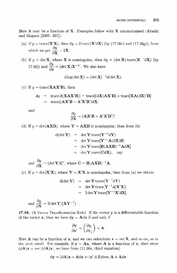
MATRIX DIFFERENTIALS 373
Here A may be a function of X. Examples follow with X unconstrained (Abadir and Magnus [2005: 3571).
(a) If y = trace(X’X), then dy = 2trace(X’dX) (by (17.56~) and (17.56g)), from 8 Y d X
which we get - = 2X.
(b) If y = det X, where X is nonsingular, then dy = (det X) trace(X-’dX) (by d Y d X
17.56j) and - = (det X)X-”. We also have
dlog(det X) = (det X)-’d(det X).
(c) If y = trace(XAX’B), then
dy = trace[d(XAX’B)] = trace[(dX)AX’B] + trace[XA(dX)’B]
= trace[(AX’B + A’X’B’)dX]
and
3 = (AX’B + A’X’B’)’. dX
(d) If y = det(AXB), where Y = A X B is nonsingular, then from (b)
d(det Y) = det Y trace(Y-’dY)
= det Y trace[Y-’A(dX)B]
= det Y trace[B(AXB)-’AdX]
= det Y trace( CdX), say,
dY dX
and - = (det Y)C’, where C = B(AXB)-’A.
( e ) If y = det(X’X), where Y = X’X is nonsingular, then from (a) we obtain
d(det Y) = det Y trace(Y-’dY)
= det Y trace[Y-’d(X’X)]
= 2 det Y trace[Y-’X’dX]
8Y d X
and - = 2(det Y)(XY-’).
17.58. (A Vector Transformation Rule) If the vector y is a differentiable function of the vector x, then we have dy = Adx if and only if
””=(!@)=A. dX’
Here A can be a function of x, and we can substitute x = vecX, and so on, as in the next result. For example, if y = Ax, where A is a function of x, then since (dA)x = vec [(dA)x], we have from (11.16a, third equation)
dy = (dA)x + Adx = (x’ ~3 1)dvec A + Adx
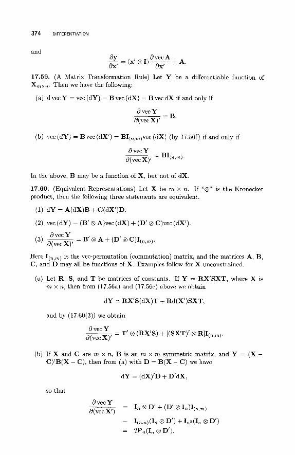
374 DIFFERENTIATION
and a vec A
= (x’ 8 I)----- + A. dy dX’ dX’
17.59. (A Matrix Transformation Rule) Let Y be a differentiable function of X,,,,. Then we have the following:
(a) d vec Y = vec (dY) = B vec (dX) = B vec d X if and only if
a vec Y = B.
d(vec X)’
(b) vec (dY) = B vec (dX’) = BI(,,,)vec (dX) (by 17.56f) if and only if
d vec Y d(vec X)’ = BI(n,m).
In the above, B may be a function of X, but not of dX.
17.60. (Equivalent Representations) Let X be m x n. If “8” is the Kronecker product, then the following three statements are equivalent.
(1) d Y = A(dX)B + C(dX’)D.
(2) vec (dY) = (B’ @ A)vec (dX) + (D’ @ C)vec (dX’).
Here I(,,,) is the vec-permutation (commutation) matrix, and the matrices A, B, C, and D may all be functions of X. Examples follow for X unconstrained.
(a) Let R, S, and T be matrices of constants. If Y = RX’SXT, where X is m x n, then from (17.56a) and (17.56~) above we obtain
d Y = RX’S(dX)T + Rd(X’)SXT,
and by (17.60(3)) we obtain
d vec Y d(vec X)’
= T’ @ (RX’S) + [(SXT)’ @ R]I[,,,).
(b) If X and C are m x n, B is an m x m symmetric matrix, and Y = (X - C)’B(X - C), then from (a) with D = B(X - C ) we have
d Y = (dX)’D + D’dX,
so that
- - d vec Y d(vec X’)
- - - -
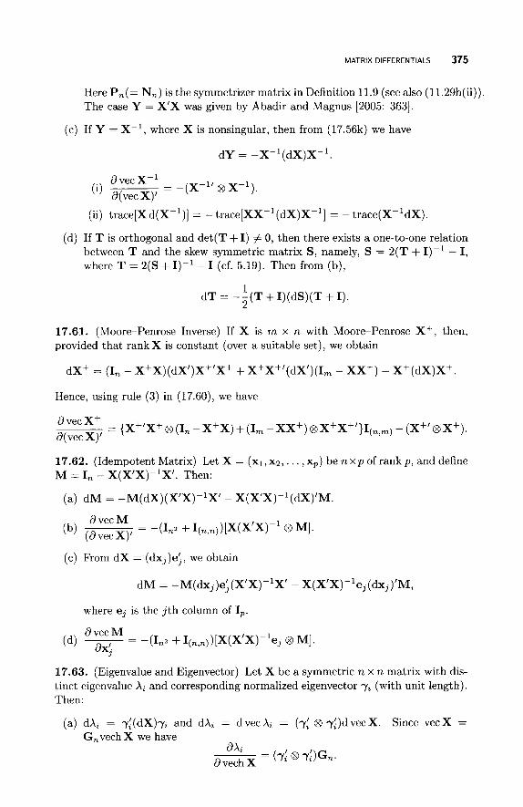
MATRIX DIFFERENTIALS 375
Here P,(= N,) is the symmetrizer matrix in Definition 11.9 (see also (11.29h(ii)). The case Y = X’X was given by Abadir and Magnus [2005: 3631.
If Y = X-’, where X is nonsingular, then from (17.56k) we have
d Y = -X-’(dX)X-’.
(ii) trace[)( d(X-’)] = - trace[XX-’(dX)X-’] = - trace(X-’dX).
If T is orthogonal and de t (T +I) # 0, then there exists a one-to-one relation between T and the skew symmetric matrix S, namely, S = 2(T + I)-’ - I, where T = 2(S + I)-’ - I (cf. 5.19). Then from (b),
1 d T = - z ( T + I ) (dS)(T + I).
17.61. (Moore-Penrose Inverse) If X is m x n with Moore-Penrose X+, then, provided that rankX is constant (over a suitable set), we obtain
dX+ = (I, - X+X)(dX’)X+’X+ + X+X+’(dX’)(I, - XX’) - X+(dX)X+.
Hence, using rule (3) in (17.60), we have
d vec X+ d(vec X)’
17.62. (Idempotent Matrix) Let X = ( X ’ , X ~ , . . . , x,) be n x p of rank p , and define
= {X+’X+@(I,-X+X)+(I,-XX+)@x+X+’}I(,,,) - (X+’@x+).
rn - X(X’X)-’X’. Then:
d M = -M(dX)(X’X)-’X’ - X(X’X)-’(dX)’M.
- d vec M
(d vec X)‘ - -(In2 + I(,,,))[X(X’X)-’ C3 MI.
From d X = (dx,)ei, we obtain
d M = -M(dx,)e;(X’X)-’X’ - X(X’X)-’e,(dx,)’M,
where ej is the j t h column of I,.
17.63. (Eigenvalue and Eigenvector) Let X be a symmetric n x n matrix with dis- tinct eigenvalue Xi and corresponding normalized eigenvector yi (with unit length). Then:
(a) dXi = y,’(dX)yi and dXi = dvecXi = (7: @ yI)dvecX. Since vecX = G,vech X we have
dXa d vech X -- - (rl@ cy,l)Gn.
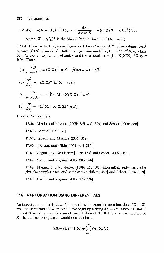
376 DIFFERENTIATION
ax, 8 vech X
(b) dyi = -(X - XiIn)+(dX)yi and ~ = - { ~ i @ (X - XiI,)+}G,,
where (X - X,I,)+ is the Moorepenrose inverse of (X - &In).
17.64. (Sensitivity Analysis in Regression) From Section 20.7.1, the ordinary least squares (OLS) estimate of a full-rank regression model is p = (X’X)-lX‘y, where X = (xl,x2,. . . ,xp) i snxpof rankp , andtheresidualisr = (In-X(X’X)-lX’)y = My. Then:
Proofs. Section 17.8.
17.56. Abadir and Magnus [2005: 355, 362, 3691 and Schott [2005: 3561.
17.57b. Mathai [1997: 711
17.57~. Abadir and Magnus [2005: 3591.
17.60d. Deemer and Olkin [1951: 364-3651,
17.61. Magnus and Neudecker [1999: 1541 and Schott [2005: 3611.
17.62. Abadir and Magnus [2005: 365-3661,
17.63. Magnus and Neudecker [1999: 159-160, differentials only; they also give the complex case, and some second differentials] and Schott [2005: 3691.
17.64. Abadir and Magnus [2006: 375-3761,
17.9 P ERTU R BAT I 0 N US I N G D I FFER E N TI A LS
An important problem is that of finding a Taylor expansion for a function of X+dX, when the elements of dX are small. We begin by writing dX = EY, where E is small, so that X + EY represents a small perturbation of X. If f is a vector function of X, then a Taylor expansion would take the form
W
f ( X + t Y ) =f (X)+-pgg, (X,Y) , 2 = 1
MATRIX LINEAR DIFFERENTIAL EQUATIONS 377
where gz(X,Y) represents some vector function of X and Y . Similarly, if we have a matrix function F, then the expansion would take the form
cc
F(X + EY) = F(X) + C eZG2(X, Y ) , z = 1
where G, is now a matrix function. Schott [2005: section 9.61 demonstrated the method with several examples, and some of the results of these are given below. He also demonstrated how the method can be used for finding differentials and, ultimately, Jacobians.
17.65. Suppose that X is nonsingular and F(X) = X-'. Then
(X + dX)-' = X-l - X-l(dX)X-l + X-l(dX)X-'(dX)X-'
-X-l(dX)X-l(dX)X-l(dX)X-l + . . . . 17.66. Let X be a real symmetric n x n matrix with spectral decomposition X = QAQ', where A = diag(A1, Xz, . . . , A,) and A, = A,(X) is a distinct eigenvalue of X corresponding to the eigenvector q,, the i th column of Q. Let Xz(X + dX) and yz be the eigenvalue and corresponding eigenvector of X + dX. If d X = Q'WQ, where W is "small" and symmetric, then we have the following:
(a) X,(X + dX) = A, + q:Wq, + . . .. (b) rt(X + dX) = qz - (Z - X,I,)+Wq, + . . ..
Proofs. Section 17.9.
17.65-17.66. Schott [2005: 3691.
17.10 MATRIX LINEAR DIFFERENTIAL EQUATIONS
17.67. If x = x ( t ) is an n x 1 vector with elements that are functions o f t and A is an n x n constant matrix, then
-- ax(t) - A X ( ~ ) , x(0) = xo at
has a formal solution x = eAt XO. If A is not a diagonal matrix, then the system of equations is said to be coupled. This coupling, which links azi(t)/at to the other components of x(t), makes the solution harder t o actually find. If A can be transformed to a diagonal or near diagonal form, then the problem may be easier to solve. For example, if A = SJoS-', where JO is the Jordan canonical form of A, then the differential equation becomes
= Joy(t), at Y(0) = Yo,
where x(t) = S y ( t ) and yo = S-'XO. However, if A is diagonalizable, then Jo = diag(X1,. . . , A,), where the X i are the eigenvalues of A. The transformed equations are now uncoupled and have solutions
y z ( t ) = yz(O)eA%t, 2 = I , 2 , . . . ,n.
378 DIFFERENTIATION
For further details see Horn and Johnson [1985: 133-1341.
17.68. If x = x(t) , then ~ ax(t) = Ax(t) + b(t) and x(t0) = xo has solution a t
t x(t) = eA(t-to)xo + eAt ePA"b(s)ds. Lo
Further details are given by Seber and Wild [1989: section 8.31. For solutions of the more general case
A% at + Bx(t) = b(t),
where A may be nonsingular, see Campbell and Meyer [1979: section 9.21.
17.69. If X = X(t) is an m x n matrix with elements that are functions o f t , then
ax(t) = AX + XB, X(0) = Xo a t
has solution X = eAt XO eBt.
Proofs. Section 17.10.
17.68. Bellman [1970: 1731 and Gantmacher [1959: 116-124, 153-1541.
17.69. Graham [1981: 411 and Horn and Johnson [1991: 503-5111,
17.11 SECOND-ORDER DERIVATIVES
Second-order derivatives are often required for determining the stationary values of a function. Below we give some techniques for finding Hessians.
Definition 17.8. Let f ( X ) be a scalar function of the m x n matrix X that is twice differentiable inside the domain of f. Then the Hessian of f is defined to be
If X is a vector, say x, then
0 2 f ( X ) = - - - (&)
If Y is a matrix function of X, we also define the second dzfierential d2Y = d(dY); and in deriving this in applications, we note that d2X = 0. For some analytical details see Abadir and Magnus [2005: chapter 131, Harville [1997: section 15.11, Magnus and Neudecker [1999: chapter 61, and Nel [1980]. A number of examples are given by Nel [1980: section 7.21.
SECOND-ORDER DERIVATIVES 379
17.70. The Hessian as defined above is symmetric.
17.71. (Identification Rules)
(a) d2f(X) = (vecdX)’B(vecdX) if and only if 0 2 f ( X ) = i ( B + B’), where B may depend on X but not on dX.
For example, if f (X) = trace(AXBX’C), where A, B, and C are square ma- trices (not necessarily of the same size) of constants, then taking differentials twice and setting d2X = 0 and d(dX)’ = 0 we have, interchanging “d” and “trace”, and noting that traceF = traceF‘,
d f (X) = trace[A(dX)BX’C + AXB(dX)’C],
and
d2f(X) = 2 trace[A(dX)B(dX)‘C]
= 2 trace[(dX)’CA(dX)B
= 2(vecdX)’(B’ 8 CA)(vecdX),
since trace(D’E) = (vecD)’vecE) and vec (DEF) = (F’ 8 D)vecE. Here “@” is the Kronecker product. We thus have from (a) the following rule:
(b) d2f(X) = trace[A(dX)B(dX)’C] if and only if
02f (X) = a(B’ @ C A + B 8 A’C’).
Similarly, by using trace(FG) = trace(GF), we see that
d2f (X) = trace[B(dX’)C(dX)] if and only if
02f (X) = a(B’ @ C + B @ C’).
For example, if f ( X ) = trace(X’AX), then d2f(X) = 2trace[(dX’)AdX) and
0 2 f ( X ) = I 8 ( A + A’).
(c) d2f(X) = trace[B(dX)C(dX)] if and only if
02f (X) = iI(m,n)(B’ 8 C + C’ 8 B),
where X is m x n and I(m,n) is the commutation (vec-permutation) matrix. We have the following examples for n x n X.
(i) If f ( X ) = trace(X-l), then d2f(X) = 2 t ra~e[X-~(dX)X-’dX] and
0 2 j ( X ) = I(n,n)(x’-2 8 x-l + x’-l 8 X P ) .
(ii) If f (X) = det X , then
V2f(X) = - detX[I(,,,)(X’-’ 8 X-’) - (vecX’-’)(vecX’-’)’].
380 DIFFERENTIATION
(d) We also have the following special case for vectors.
d2 f (x ) = (dx)’A(dx) if and only if
For example, if f ( x ) = x’Bx, where B is a symmetric constant matrix, then d f = 2x’Bdx and d2f = 2(dx)’Bdx. Here A can be a function of x.
V2f(x) = ;(A +A’).
17.72. Suppose X has L-structure (e.g., is symmetric or triangular) so that vec X = A+(X) (cf. Section 18.3.5 for notation), then
If X is symmetric and n x n, then +(X) = vechX and A = G,, the duplication matrix.
We demonstrate the above theory with the example f (X) = trace(X-’). From (17.71c(i)) we obtain
V2f(X) = qn,,)(X’-1 @ x-2 + x ’ - 2 8 x-1). If X is symmetric, then
since I(n,n)A = I(,,,)G, = G, = A, by (11.29d).
17.73. Let F(t), with r , sth elements frs(t), be a nonsingular matrix function of L.
- - a2 det F atiatj
(detF) [ trace ( F-l- ::Ed) +trace ( F - I ~ ) trace ( F - 1 ~ 1
a2 log(det F) at&,
VECTOR DIFFERENCE EQUATIONS 381
17.74. Let d(8 ) = det[X(O)’X(8)], where X is n x p of rank p for 8 E 0, and let k ( 8 ) = logd(8). Then from (17.12),
where X, = dX/dO,. Also
d 2 k ( 8 ) dO,dO, - trace(X+X,X+X,) + trace[X+(X+)’Xk(I, - XX+)X,]
k,, =
=
+ trace(X+X,,),
where X+ is the Moore-Penrose of X . The Hessian H(8) = (h,,) of d(8)is given bY
Proofs. Section 17.11.
17.70. Magnus and Neudecker [1999: 105-1061.
17.71a. Abadir and Magnus [2005: 3531 and Magnus and Neudecker [1999: 1901.
17.71b. Magnus and Neudecker [1999: 192-1931.
17.71~. Abadir and Magnus [2005: 380-3811 and Magnus and Neudecker [1999: 1921.
17.71d. Abadir and Magnus [2005: 3531
17.72. Magnus [1988: 1551.
17.73. Harville [1997: section 15.91.
17.74. Bates and Watts [I9851 and Seber and Wild [1989: 5431.
17.12 VECTOR DIFFERENCE EQUATIONS
Definition 17.9. The vector difference equation
A o ~ t + Aiyt-1 + . . . + A,yt-, = g( t ) ,
with A0 nonsingular and all vectors n-dimensional functions o f t , is called an rth- order vector dzfference equation with constant coeficients. Since A0 is nonsingular, we can set A0 = I d without loss of generality. Difference equations arise in discrete time stochastic processes and in iterative procedures that converge. The case when A0 is singular can be handled using the Drazin inverse of A0 (Campbell and Meyer [1979: 181-184]).
382 DIFFERENTIATION
17.75. The above difference equation can be reduced to a first-order equation as follows. Let zt = (yi ,y$-l , . . . , yiPr+’)’ and
-A1 -A2 . . . -A,-’ -Ar
0 O ) . B = ( Id 0 . . . 0 0 0 . . . Id
Then zt = Bzt-l +el @ g ( t ) , where el is an r-dimensional vector (1,0,. . . , 0)’ and “8” is the Kronecker product. The solution of this was studied by Dhrymes [2000: 175-1781, He applies it t o the general linear structural econometric model.
17.76. If xt = Axt-’ + d, where A and xo are known, then provided that At + 0 as t -+ cc and (I - A)-’ exists, we have xt = Atxo + (I - At)(I - A)-’d and xt + (I - A)-’d as t + 00.
Definition 17.10. (Linear Stationary Iterations) Let Ax = b, with A n x n and expressible in the form A = M - N, where M-’ exists. Let H = M-lN, the iteration matrix, and let d = M-lb. Given an initial n x 1 vector x ( ~ ) , then a linear stationary iteration is
~ ( k ) = H~(k-1) + d, IC = 1 ,2 ,3 , . . . .
17.77. Given the notation above, if p(H) < 1, where p is the spectral radius, then A is nonsingular and
lim x ( k ) = x = A-’b
for every initial vector x ( ~ ) . For details and methods see Meyer [2000a: 620-6261.
Proofs. Section 17.12.
k - c c
17.76. Searle [1982: 2891.
17.77. Meyer [2000a: 6211.
CHAPTER 18
JACOBIANS
Jacobians play a fundamental role in statistical distribution theory. Formulae for Jacobians and their proofs are given in many places, especially in the appendices of statistics books. In the case of complicated transformations, it is not always clear what the sign of the Jacobian is as it will depend on how the variables are ordered. Fortunately, the ordering only affects the sign of the Jacobian, which usually does not matter as in applications we are mainly interested in the absolute value of the Jacobian.
18.1 INTRODUCTION
Before listing a number of results, we look at the meaning of a Jacobian and give a number of different techniques for finding Jacobians.
Definition 18.1. Suppose f : x -+ y = f(x), where x and y belong to Rn, is a one- to-one (bijective) differentiable function, i.e., it has an inverse function g = f - l .
Then axlay’ = (asi/ayj) is called the Jacobian matrix of the transformation x + y, and its determinant
Jx + = det (&) is called the Jacobian of the transformation. (Some authors call the absolute value IJx + y l the Jacobian.) For further comments on this definition see Section 17.7.
A Matrix Handbook for Statisticians. By George A. F. Seber Copyright @ 2008 John Wiley & Sons, Inc.
383
384 JACOBIANS
In the above definition we want to differentiate x with respect to y, so it is more natural to use x = g(y), as does Muirhead [1982: chapter 21, for example. However, as most of the references use y = f (x) , I have decided to stay with the latter in this chapter. As it can be a source of possible confusion, Daniel L. Solomon gives the following mnemonic rule (Searle [1982: 3391) to help get the order of the variables right: If “0” represents the old coordinates (x) and “n” represents the new cordinates (y), then Jo -+
If we interchange two elements of y, we change the sign of Jy+x. Since, in prac- tice, we are generally more interested in the absolute value of the Jacobian, I Jy-xl, it does not matter in what order we list the elements of x and y. Several authors- for example, Mathai [1997], whom I will refer to frequently in this chapter-get around this problem by stating that the sign of a particular Jacobian should be ignored. I shall tend to use absolute values throughout.
As already mentioned, if we want to differentiate x with respect to y, we can endeavor to express the transformation in the form x = g(y). However, it may be easier to find Jy -+ x first as JX + Y = J& x. To see this, we have x = g(f(x)) and
is correct, but Jn ---$ is not (spells no).
Then
We note that Jy --+ x will be expressed in terms of x, which in applications usually has to be replaced by its function of y. For example, two important statistical applications of Jacobians are (i) change of variables in integratioqthat is,
and (ii) probability density functions for functions of random variables, namely
M Y ) = f X k ( Y ) ) l J X + yl.
If x and y are replaced by matrices with Y = F(X), we define
and, if X and Y are symmetric or lower-triangular, we define
JX-Y = Jvech x-vech Y = det
For upper-triangular matrices we can use vech (XI). In order to evaluate the above Jacobians, various properties of the Kronecker
product and of the vec and vech operators are required from Chapter 11. In this chapter we shall concentrate on finding JY,X or IJy-xl, which can then be in- verted. Unless otherwise stated, all matrices and scalars are real. We now give some techniques for finding Jacobians; some of these techniques are demonstrated by Olkin [2002].
METHOD OF DIFFERENTIALS 385
18.2 METHOD OF DIFFERENTIALS
Differentials were introduced in Section 17.8 along with some rules that provide a powerful method for finding Jacobians.
18.1. A key result from (17.28) for vectors is as follows. If d y = Adx, where A may be a function of x, then
dy = A and Jy+x = det A . ax'
In the case of matrices, if d v e c Y = B d v e c X , then
a vec Y a(vec X)'
= B and JY-X = d e t B ,
where B may be a function of X. Also dvec X = vec (dX).
18.2. We recall the following equivalent statements from (17.60), where X is m x n.
(1) d Y = A(dX)B + C(dX')D.
(2) vec (dY) = (B' @ A)vec (dX) + (D' @ C)vec (dX'), or, equivalently,
d vec Y = { (B' 8 A) + (D' @ C)I(n,ml}d vec X.
When the above hold, we see from (2) and (3) that
JY-X = JVeCY-vecX = Jdvecy-dvecx
We demonstrate how these results can be used by working through two examples.
Example 1 Let Y,,, = AmxmXmxnBn,, , where A and B are nonsingular. Then d Y = A(dX)B and vec (dY) = (B' @ A)vec (dX). Using (17.1l(ii)), we get
Jy-x = det(B' 8 A) = (det B)m(det A)".
Thus, Jx-y = (det B)-m(det A)-".
Example 2 Let Y = X-', where X is a nonsingular n x n matrix. Since YX = I,, we have 0 = d(YX) = Y d X + (dY)X, or d Y = -X-l(dX)X-l. Thus, from Example 1 with A = -X-' and B = X-', we have
JY-X = (-1)nZ(detX)-2",
and JX-Y = (-l)nZ(detY)-2n.
18.3 FURTHER TECHNIQUES
In addition to the method of differentials, there are a number of other useful related techniques that we now describe.
386 JACOBIANS
18.3.1 Chain Rule
One useful technique makes use of the chain rule (17.21). This rule leads to the result that if we have the transformations x - y and y -+ z, then JX --+ z - JX --+ y J y -+ z, i.e., Jacobians multiply. If the Jacobian of x -+ z is hard to derive, it may be possible to find an intermediary variable y such that Jx --f y and J y -+ z are easy to find. This method was used frequently by Deemer and Olkin [1951] and Olkin [1953], and several examples of it appear later.
-
18.3.2
This elegant technique is described in detail by Muirhead [1982: chapter 21 and used extensively by Mathai [1997] . We assume that y and x are n x 1 vectors, and we introduce a skew-symmetric product ‘‘A” of differentials called the exterior or wedge product, satisfying (i) dyi A dyj = -dyj A dyi and (ii) dyi A dyi = 0 (a consequence of (i)). To evaluate det(ay/ax’), we begin with
Exterior (Wedge) Product of Differentials
and multipy these together using the above two properties of the exterior product to get
dy1 A dy2 A . . . A dy, = det - dxl A dx2 A . . . A dx,. ( Z ) This result is readily demonstrated for n = 2. We have
8 Y l dy1 A dy2 = ( g d x 1 + -dx2 8x2
-. dYl dY2
ax, 8x1 ax l ax2 *dxl A dxl + - . -dxl A dx2 - -
aYl dY2 dYl dY2 ax2 ax1 ax2 ax2
+- . - d ~ 2 A dxl + - . - d ~ 2 A d ~ 2
= det - dxl Adx:!. (2) We shall define the wedge product for a vector x as
d,x = AY==,dxi.
This approach extends to matrices by setting y = vecY and defining d,Y = Ai,jGDdyij, where 2, denotes the ordered set of distinct elements of Y, ordered ac- cording to y . I have deliberately made this notation different from that of Muirhead
FURTHER TECHNIQUES 387
[1982] and Mathai [1997] to avoid confusion, because they use brackets like (dX) with opposite meanings.
If Y is symmetric or lower-triangular, we can use y = vechY for the distinct elements of Y and define d,Y = d,y = d,vechY. In the case of a skew-symmetric matrix, the diagonal elements are ignored, as they are zero. However, as already noted, the order in which the distinct elements of these matrices are listed is not important in applications.
18.3. It follows from the above that if vecY = y and vecX = x, then
d,Y = d e t - d,X. (2') Since, as already mentioned, the order of the variables can be arbitrary, we have
d,Y = (det C)d,X ==+ IJy-xl = I det CI.
Example 3 Let (y1,y2 , . . . , yn) = Y = A X = (Ax1,Axz , . . . , Ax,). Then, from (18.1), d,yi = (det A)d,xi, so that d,Y = A:==,d,yi = (det A)"d,X, and lJyCxI = I det A[". Alternatively, vec Y = diag(A, A , . . . , A)vec X and, from (18.1), I det CI = I det{diag(A, A , . . . , A)}I = I det Al", as before.
Example 4 Let Y = BX, where the matrices are all n x n lower-triangular matrices so that (y1,y2,. . . , y n ) = (Bxl,Bxz,. . . ,Bx,). For T = 1 , 2 , . . . , n, let y(r) = (yr,?, ~ ~ + l , ~ , . . . , Y,,~) ' be yT without its leading zeros; x ( ~ ) is similarly defined. Note that y(n) = yn,, = bn,nxn,n = bn,nx(n). Then
a, = det (-) 8yn.n = b,,n axn,n
and so on. Hence
r=l r=l
18.3.3 Induced Functional Equations
Olkin and Sampson [1972] described a method whereby one sets up an equation satisfied by the Jacobian and then solves the equation.
Example 5 Suppose Y = AXA', where A is nonsingular and Y is symmetric. To find the Jacobian of this transformation, let Z = BYB', where B is nonsingular and Z is symmetric, so that Z = ABX(AB)'. Then
IJZ-XI = IJZ-Yl ' IJY-XI.
388 JACOBIANS
As the transformation is linear in X, IJy-xI is a positive function of A above, say h(A). Then, by the above equation,
h(AB) = h(A)h(B),
which, for this example, has solution h(A) = I det Al", for some c. Setting A = diag(a, 1 , 1 , . . . , 1) and finding JY-X for this simple case, leads to c = n+ 1 (Olkin and Sampson (1972: 2631).
Olkin and Sampson [1972] derive solutions of the equation h(CD) = h(C)h(D) for diagonal, triangular, orthogonal, and symmetric matrices. Their paper can be referred to for details (see also Mathai [1997: 40-441 for a summary of the main results).
18.3.4 Jacobians involving Transposes
Consider the transformation Y = X', where X is an m x n unconstrained matrix. Then, by (11.18b(i)) and (11.18f(i)),
vecY = vecX' = I(,,,)vecX,
Jy,x = detI(,,,) = (-l)im(m-l)"("-l) , and IJy-xl = 1.
Example 6 Consider the transformation Y,, , = AmxnX/mxnBnxn, where A and B are nonsingular. Setting W = X' and Y = A W B , we have, from Example 1 above and the chain rule (17.21),
Jy-x = Jy-w JW-x = (det B),(det A)" (-1) am(m-l)"(n-l), In practice, we are more interested in absolute values so that we do not need to distinguish between X and X' in linear transformations like the above, as I Jw-xl =
/ J x / - x ~ = 1 and IJy-xl = I J Y - w ~ . Example 7 Suppose we know the Jacobian for the transformation Y = AX, and we want to find the Jacobian for Y = XA. Taking transposes, we obtain Y' = A'X' or W = A'Z. Then
and, by Example 6, IJy-xI = IJw~+zl . Hence the absolute value of the Jacobian for Y = X A can be obtained from the one for Y = A X by simply replacing A by A'. Example 7 is, of course, a special case of Example 6, but the method is instructive.
18.3.5 Patterned Matrices and L-Structures
Sometimes the matrices involved are "patterned" or structured in some way such as symmetric or triangular. We are therefore interested in this case where vecX (where X is m x n) will be in a linear subspace D, of Rmn. For example, if X is n x n and lower-triangular, then vecX will contain zeros in a certain pattern.
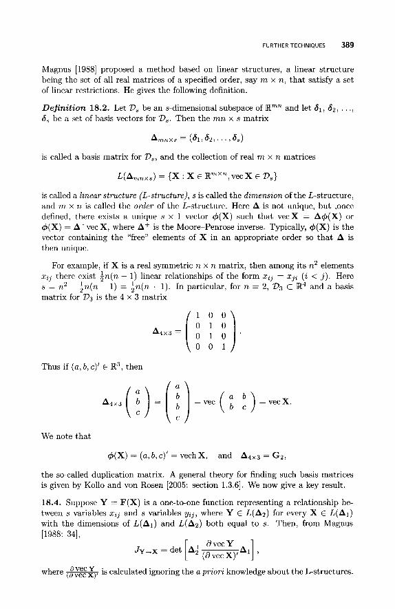
FURTHER TECHNIQUES 389
Magnus [1988] proposed a method based on linear structures, a linear structure being the set of all real matrices of a specified order, say rn x n, that satisfy a set of linear restrictions. He gives the following definition.
Definition 18.2. Let D, be an s-dimensional subspace of R”” and let 61, 62, . . ., 6, be a set of basis vectors for D,. Then the rnn x s matrix
Arnnxs = (61, 62,. ’ . Id,)
is called a basis matrix for Vs, and the collection of real rn x n matrices
L(Amnxs) = {X : X E Rmxn,vecX E D,}
is called a linear structure (L-structure), s is called the dimension of the L-structure, and m x n is called the order of the L-structure. Here A is not unique, but ,once defined, there exists a unique s x 1 vector +(X) such that vecX = A#(X) or +(X) = A+vec X, where A+ is the Moore-Penrose inverse. Typically, 4 ( X ) is the vector containing the “free” elements of X in an appropriate order so that A is then unique.
For example, if X is a real symmetric n x n matrix, then among its n2 elements zij there exist in (n - 1) linear relationships of the form xij = xji (i < j ) . Here s = n2 - in (n - 1) = in (n + 1). In particular, for n = 2, 273 c B4 and a basis matrix for D3 is the 4 x 3 matrix
1 0 0 A4x3= [ 0 1 0 0 1 0 ) .
0 0 1
Thus if (a , b, c)’ E R3, then
We note that
+(X) = (a , b, c)’ = vech X, and A4x3 = Gz,
the secalled duplication matrix. A general theory for finding such basis matrices is given by Kollo and von Rosen [2005: section 1.3.61. We now give a key result.
18.4. Suppose Y = F(X) is a one-to-one function representing a relationship be- tween s variables zij and s variables yij, where Y € L(A2) for every X € L(A1) with the dimensions of L(A1) and L(A2) both equal to s. Then, from Magnus 11988: 341,
where is calculated ignoring the a priori knowledge about the L-structures.
390 JACOBIANS
Henderson and Searle [1979: 74-76] discussed the same idea, but from a slightly different perspective. They define vecp,(Z) as the vector of the distinct elements with pattern pz, where Z = X or Y (they use XI and X2). Then
vecp,(Z) = P,vec Z and vec Z = Qzvecpz(Z) = QzPzvec Z,
where P, and Qz correspond to H and G of Section 11.5.1. In particular, P,Q, = I, Qz has full column rank, and P, = (QLQZ)-'QL is one possible choice for P,. Finally,
Derivatives for patterned matrices are also discussed by Nel [1980: section 61. Kollo and von Rosen [2005: 135-1491 develop derivatives for structured matrices, but use a derivative notation Y 8 a/aX.
We are now going to systematically list Jacobians. If the order of the variables is not well defined, IJI will be quoted instead of J .
18.4 VECTOR TRANSFORMATIONS
The following transformations between n x 1 vectors are one-to-one.
18.5. If y = Ax, where A is nonsingular, then from (17.28) we have
When A = aInr lJytxl = lain.
18.6. (Symmetric Functions) Let yi = x ( t x ) , i = 1,2, . . . , n, where x( ix) is the so-called (elementary) symmetric function representing the sum of all the products of x3 taken i at a time. Thus y1 = X I +.. . + xn, y2 = 51x2 + ~ 1 x 3 +. . . + xn-lxn, and yn = ~ 1 x 2 . . '2,. Then for each xj > 0,
n-1 n
i=l j=i+l
18.7. If
Y1 = x 1 + x 2 + . . . + x n ,
Y2 = x: +x; +". +xi,
then, for each xj > 0,
i = l j = i + l
JACOBIANS FOR COMPLEX VECTORS AND MATRICES 391
18.8. (Polar Coordinates)
(a) Consider the transformation
5 1 = T sin O1 sin 02 . . . sin sin On-lr
5 2 = T sin O1 sin O2 . . . sin cos
z3 = T sin dl sin O2 . . . cos
znP1 = rsin&cose2,
z, = Tcosel, where T > 0, 0 < Bi 5 7r (i = 1 , 2 , . . . , n - 2), and 0 < 8,-1 5 27r. Then, if e = (el, e 2 , . . . , en) / , we have
I J , ~ T, 0 I = rn-l [(sin 01)"-2(sin 0 2 ) " ~ ~ . . . sin
(b) If we reverse the order of the zi and replace Bi by - Oi in (a), we get
z1 = TsinO1,
xCj = T C ~ S ~ ~ C ~ S ~ ~ . . . C O S ~ , -,sine,, j = 2 , 3 , . . . , n - 1 ,
5 , = ~cose1cose2 . . . co~e , -1 ,
where T > 0, -$ < Oi 5 $ (i = 1,. . . ,n - a) , and -7r < 5 T . Then
IJ, ~ r , 8 1 = T ~ - ~ ~ ( c o s ~ , ) ~ - ~ ( c o s ~ , ) ~ - ~ . . .~o~e , - , l .
Proofs. Section 18.4.
18.6. Mathai [1997: 431
18.7. Mathai [1997: 451.
18.8a. Mathai [1997: 451 and Muirhead [1982: 551
18.8b. Mathai [1997: 451.
18.5 JACOBIANS FOR COMPLEX VECTORS AND MATRICES
We demonstrate the meaning of a Jacobian for complex variables using a simple example taken from Mathai [1997: 175-1761, Let y = y 1 + iy2 and x = x1 + ix2, where the x, and y z are all real n x n vectors. Consider the transformation y = Ax where A is real. Then yi = Axi for i = 1,2, and
We define the Jacobian of the transformation to be Jyl,yz+xl,xz. From (18.5) this is det B = (det A)2 (= I det AI2, say).
392 JACOBIANS
If A is complex and A = A1 + iA2, then
and we have y1 = Alxl - A2x2 and y2 = Alx2 + A2x1. Then dylldx; = A l , dyl/dx; = -A2, dyn/dx: = A2, and dy2/dxh = Al . Hence, from Section 5.1.2,
Thus the above equation is true for both the real and complex cases. When vectors are replaced by matrices, the expression Jy, ,y2+x1 ,xZ denotes
the Jacobian of the transformation, where Y1 and Y2 are written as functions of X1 and X2, or where Y = Y1 + iY2 is a function of X = X1 + 2x2, the elements of X being functionally independent. As we have seen from the above example, we can typically go from the real to the complex case by squaring absolute values of determinants or by replacing I det A1 by I det AA*I = I det AI2. We shall also see below that a term like 1xiil for a real diagonal element xii remains the same for a complex element except that I . I now refers to the modulus of a complex number.
18.6 MATRICES WITH FUNCTIONALLY INDEPENDENT ELEMENTS
18.9. If Y,,, = a x m x n r then JY-X = amn and IJy-xl = lalmn. For complex matrices the latter Jacobian becomes la(2mn.
18.10. If Y,,, = AmXmXmXnBnX,, where A and B are nonsingular then, from Example 1 above in Section 18.2,
IJy,xI = I det BI“. I det A(”.
The transformation is clearly one-to-one. In particular, if y = Ax, then
Other cases follow by setting A or B equal to the identity matrix.
by BB* in the above expressions.
18.11. Let Y = AXA’fBXB’, where all the matrices are n x n and A @ A f B @ B are nonsingular. Then vecY = (A @ A 41 B @ B)vec X, so that the transformation is one-to-one, and
If the matrices are complex, we find that we simply replace A by AA* and B
n n
where the C Y ~ and Pj are the respective eigenvalues of A and B.
18.12. Let Y = X-l, where X is n x n and nonsingular.
(a) From Example 2 in Section 18.2 above, JJy,xI = ( I det
MATRICES WITH FUNCTIONALLY INDEPENDENT ELEMENTS 393
(b) When X is complex, we replace X by XX*.
18.13. Let Y = (detX)X-l, where X is n x n, and d e t X > 0 to ensure the transformation is one-to-one.
(a) (i) If X is real, IJy,xl = (n - 1)(1 det Xl)n('L-2).
( i i ) If X is complex, then
IJY~,Y~+x~,x~I = (n - 1)21 det X12"("-2).
(b) (i) If X is real and Z = Y-' = X / d e t X , then
IJz-xI = (n - 1)1 det XIpn2.
This follows from JZ+X = Jz+yJy+x and (18.12).
(ii) When X is complex, )JZ~,Z~-X~,X~I = (n - 1)2)detXI-2nZ.
18.14. If Y = A X - l B and all matrices are n x n and nonsingular, then the transformation is one-to-one and
IJy,xI = I(det B),(det X)-2n(det A)"I.
This can be proved from (18.12) using Y = AZB, Z = X-l, and the chain rule.
18.15. Let Y = Xk, where X is n x n and nonsingular, and k is a positive integer.
(a) If X has nonzero, not necessarily distinct, real eigenvalues XI, X l , . . . , A,, then
We note that the transformation is generally not one-to-one.
(ii) If the eigenvalues are distinct, an alternative expression is given by
[&+XI = Ik"(det X)k-l i=l j=i+l
- x'c = Ik"(det X)k-l fi fi (2) A2 - x j 1 ,
i=l j#i
which, by noting that det X = n, A,, is readily shown to be the same as the expression in (i).
(b) Suppose k = 2, that is, Y = X2.
6) Fl-om (4, n n
(ii) When X is complex and the eigenvalues are distinct, then
n n
394 JACOBIANS
Proofs. Section 18.6.
18.9. Deemer and Olkin [1951: 3471 and Mathai [1997: 177-178, complex case].
18.10. Abadir and Magnus [2005: 3731, Henderson and Searle [1979: 721, and Muirhead [1982: 58 [1997: 1771. The complex case is given by Mathai [1997: 1771.
18.11. Mathai [1997: 75-77].
18.12a. Abadir and Magnus [2005: 3731 and Mathai [1997: 541.
18.12b. Mathai [1997: 1901.
18.13a(i). Abadir and Magnus [2005: 3731 and Mathai [1997: 721.
18.13a(ii). Mathai [1997: 2051.
18.14. Henderson and Searle [1979: 731 and Mathai [1997: 60-611.
18.15a(i). Henderson and Searle [1979: 731.
18.15a(ii). Mathai [1997: 981
18.15b(i). Henderson and Searle [1979: 731.
18.15b(ii). Mathai [1997: 2091.
18.7 SYMMETRIC AND HERMITIAN MATRICES
Let X and Y be n x n real symmetric matrices, unless otherwise stated. We note that if X = X1 + iX2 is Hermitian, then X1 is real symmetric and X2 is real skew-symmetric.
18.16. The following transformations are one-to-one.
(a) If Y = a x , then IJy-xl = lan(n+1)/2 I . (b) If Y = AXA', where A is nonsingular, then [ [ & + X I = (I detA)I"+'.
(c) If Y = AX-lA', where A and X are nonsingular, then
IJy+x) = I (detA)"+l(detX)-("")(.
(d) If X = X1 + iX2 is Hermitian, then Y = Y1 + iY2 = AXA* is Hermitian and I J Y ~ , Y ~ + x ~ , x ~ ~ = IdetAl2".
18.17. Let A and B be real nonsingular matrices, and assume that A 8 A 3~ B 8 B are nonsingular.
(a) The transformation Y = AXA' f BXB' is one-to-one since, from (11.30),
vechY = [H(A 8 A f B 8 B)G]vechX
SYMMETRIC AND HERMITIAN MATRICES 395
The matrix in square brackets is nonsingular because, from (11.29~) and (11.29g), H has full row rank and G full column rank.
(i) If A, ( i = 1,2, . . . , n) are the eigenvalues of AB-l, then
2x1 j = i
(ii) Alternatively, if ai and B, respectively, then
(i = 1,2, . . . , n) are the eigenvalues of A and
When B = 0, it can be shown that the above result reduces to (18.16b).
(iii) If A and B are lower-triangular with respective diagonal elements a,, and b,,, then
n n
i=l j = i
This is the same as (ii) as the diagonal elements of a triangular matrix are its eigenvalues.
(b) If Y = AXB' + BXA', then
n n
where X i ( i = I, 2 , . . . , n) are the eigenvalues of AB- l . We need B@A+A@B to be nonsingular for the transformation to be one-to-one.
18.18. Suppose Y = X-l , where X is nonsingular and symmetric.
(a) From (18.16~) with A = I, IJy-xl = I det
(b) If X = X1 + 2x2 is Hermitian, then Y = Y1 + iY2 is also Hermitian and
IJy1,y2-xlrx21 = I det(XX*)I-n = I det XI-2n.
18.19. Let Y = (det X)XP1, where X is positive definite. (The latter condition is sufficient for the transformation to be one-to-one.)
(a) We have:
(i) det Y = (det X)n-l and
IJy-xl = (n - l)(det X)(n+1)(n-2) /2 .
(ii) If X = X1 + 2x2 is Hermitian and positive definite, and Y = Y1 + ZYz , then
I J Y ~ , Y ~ - X ~ , X ~ I = (n - I)l det
396 JACOBIANS
(b) Suppose Z = Y-l = X / d e t X . Then
(i) IJz+xI = (n - 1)1 detXI-n(n+1)/2.
(ii) If X = XI + iX2 is Hermitian and positive definite, and Z = Z 1 + iZ2, then
IJz1,zz-x1,x21 = (n - 1)1detXI-n2.
18.20. Let Y = Xk, k = 2,3, . . ., and let X i (i = 1,2, . . . , n) be the eigenvalues of X.
i = l j = i + l
where
(ii) If the eigenvalues are di
IJY-XI =
- -
tinct, then k"(det X)k-l = ny kX;-l and z=1
n n
n n k
(b) When k = 2 we have:
(i)
n n
The transformation Y = X2 is generally not one-to-one.
(ii) When X = XI + 2x2 is Hermitian, and Y = Y 1 + i Y 2 , then
7 1 7 1
I J Y ~ , Y ~ - X ~ , X ~ I = 2" I det XI n n [ X i + X j I 2 . i = l j = i + l
18.21. If Y = XAX, where A is symmetric, and X i (i = 1 , 2 , . . . , n) are the eigenvalues of XA, then, since det(XA) = ni Xi , we have
n n n n
If A and X are positive definite and the X i are such that Xi > . . . An > 0, then the transformation is one-to-one.
SKEW-SYMMETRIC AND SKEW-HERMITIAN MATRICES 397
Proofs. Section 18.7.
18.16a. Mathai [1997: 321
18.16b. Abadir and Magnus [2005: 3731, Magnus [1988: 1281, and Mathai [1997: 321.
18.16~. Mathai [1997: 601.
18.17a(i). Magnus [1988: 1281
18.17a(ii). Mathai [1997: 75-77]
18.17a(iii). Magnus [1988: 1281.
18.17b. Magnus [1988: 1281.
18.18b. Mathai [1997: 1901.
18.19a(i). Deemer and Olkin [1951: 357, theorem 4.4; they also give the Jacobian of Y-' in corollary 4.41, Magnus [1988: 1281, and Mathai [1997: 741.
18.19a(ii). Mathai [1997: 2061
18.19b(i). Mathai [1997: 751.
18.19b(ii). Mathai [1997: 2061.
18.20a(i). Magnus [1988: 1281.
18.20a(ii). Henderson and Searle [1979: 791 and Mathai [1997: 981
18.20b(i). Mathai [1997: 66, 691.
18.20b(ii). Mathai [1997: 2091.
18.21. Magnus [1988: 1281 and Mathai [1997: 701.
1 8.8 SKEW- SY M M ET R I C A N D SKEW- H E R M IT I A N MATRICES
Let X and Y be n x n matrices with X real skew-symmetric, that is, X' = -X. Then, for the following transformations, Y is also skew-symmetric. Note that if X = X1 + 2x2 is skew-Hermitian, then X1 is real skew-symmetric and X2 is real symmetric.
18.22. If Y = a x , then lJy,xI = l ~ l ~ ( " - ' ) / ~ .
18.23. Let Y = AXA'. Then the following hold.
(a) I J Y - x I = (I det A/)"-'.
(b) If X = X1 + 2x2 is skew-Hermitian and Y = Y1 + iY2 = AXA*, then Y is skew-Hermitian and
IJy-xl = I det(AA*)l" = I det
398 JACOBIANS
which is the same as for the Hermitian case (cf. 18.16d).
18.24. Let A and B be nonsingular, and let X i ( i = 1 , 2 , . . . n) be the eigenvalues of AB-'.
f l , "_ , , , ( l+XiXj) l . (a) If Y = A X A ' f B X B ' , then IJx-YI = I (detB)"-' If A and B are lower-triangular, then
n n
2 = 1 j=z+l
The above transformations are one-to-one if ( A @ A f B @B) are nonsingular.
(b) If Y = AXB' + BXA', then
n n
i=l j=i+l
The above transformation is nonsingular if (B @ A + A @ B) is nonsingular.
18.25. Let Y = AX-'A', where A is nonsingular.
(a) IJy-xl = I det AIR-ll det
(b) If Y = X-', we can set A = I in (a).
(i) IJy-xl = I detXI-(n-l).
(ii) If X = X - 1 + iX2 is skew-Hermitian and Y = Y1 + iY2, then ( J Y ~ , Y ~ ~ X ~ , X ~ ~ = Idet(XX*)l-n = IdetXI-2n, the same as for the Hermitian case of (18.18b).
18.26. If Y = (det X)X-', where det X # 0, then
IJy-xl = (n - 1)1 det XI("-')(np2)'2.
18.27. Let Y = Xk, k = 3 , 5 , . . ., and let A, ( i = 1 ,2 , . . . , n) be the eigenvalues of X. Then we have
n n
where
If Y = X2, then Y is symmetric and the transformation is not one-to-one.
18.28. If Y = X A X , where A is skew symmetric, then
n n
z=1 j = z + 1
where X, (i = 1 , 2 , . . . , n) are the eigenvalues of X A .
TRIANGULAR MATRICES 399
Proofs. Section 18.8.
18.22. Mathai [1997: 361.
18.23~~. Deemer and Olkin [1951: 3491, Magnus [1988: 1351, Mathai [1997: 361, and Olkin and Sampson [1972: 2631.
18.2313. Mathai [1997: 1851.
18.24. Magnus [1988: 1351.
18.25a. Mathai [1997: 601.
18.25b(ii). Mathai [1997: 1901.
18.26. Magnus 11988: 1361.
18.27. Magnus [1988: 1361.
18.28. Magnus [1988: 135).
18.9 TRIANGULAR MATRICES
Any matrix with a “tilde”-for example, X-will denote a n x n nonsingular lower- triangular matrix. Results for upper-triangular matrices can be obtained by taking transposes. In what follows we assume that the elements in the lower triangle of X are unconstrained (functionally independent). Also, the product of lower- triangular matrices is lower-triangular, and the inverse of a lower-triangular matrix is also lower-triangular.
18.9.1 Linear Transformations
18.29. Let Y = PXQ, where P and Q are lower-triangular and nonsingular. - - -
(a) If the matrices are all real,
n n-z+l
I J Y 3 = I I I P f , c l i i I. i= 1
We get special cases by setting P = I, or Q = I,.
(b) If the matrices are all complex (i.e., Y = Y 1 + i Y 2 , etc.), then we have the following results.
- (i) If Y = PX, then IJq,,qZ+klrk21 = n7=l
(ii) If Y = XQ, then [Jql,qz+kl,k21 =
(or n:=l Ipii12i-1 if the pii’s and z i i ’ s are real).
Iqii12(n--i+1)
(or ny=l Iqii12(n--i)+1 if . the qi i ’s and zii’s are real).
400 JACOBIANS
(c) Given real matrices, if X, and therefore Y , has fixed diagonal elements, then
n
i= 1
(d) Given real matrices, if Y = a x , then
When the matrices and a are complex, we get I u ~ ~ ( ~ + ’ ) . 18.30. (Upper-Triangular) If Z = P’X’Q’, where P and Q are nonsingular, then 2; is upper-triangular.
(a) For real matrices, n
i=l
By interchanging P and Q, taking the transpose, and noting that lJ%+%l = lJk-g,l, we see that the above result is equivalent to (18.29a), but for upper- triangular matrices.
(b) The results for complex matrices are similar t o those given in (18.29a) by transposing, and interchanging (i) and (ii).
- - I - - - 18.31. Let Y = PXQ + RXS, where the matrices are all real.
n i
z=1 J=1
The transformation is one-to-one if Q’ @ P + S’ @ R is nonsingular. Also, if R = 0,
n-z+1 fi f i ( P Z 2 q J J ) = Pll(P22qllP22q22)(P33qllP33q22P33433) ‘ ’ . = f i P h Z Z I
z=13=1 2= 1
as in (18.29a).
(b) If X has fixed diagonal elements, then
n 2-1
Proofs. Section 18.9.1.
18.29a. Magnus [1988: 1311, Mathai [1997: 291, and Olkin and Sampson [1972: 2641.
18.29b. Mathai [1997:179- 1801.
18.29~. Magnus [1988: 1371.
TRIANGULAR MATRICES 401
18.29d. Mathai (1997: 1791
18.30a. Mathai [1997: 291.
18.30b. Mathai [1997: 180-1811.
18.31a. Magnus [1988: 1321
18.31b. Magnus [1988: 1371.
18.9.2 Nonlinear Transformations of X
All matrices are real, unless otherwise stated.
18.32. Let Y = XPX. - - -
n n
(a) lJ-i.+xl = 2n l(det P)(det X) n n ( p i i ~ i i + pjjsj j)( . i=l j=i+l
(b) If X has fixed diagonal elements, then
n n
18.33. Let Y = X-I.
(a) We have n
i=l
(b) If X has fixed diagonal elements, then
18.34. Let Y = (detX)X-', where Y and X are both lower- or both upper- triangular matrices.
(a) Then det Y = (det X)n-l.
(4
I J - Y-x - 1 = (n - 1)1 detXI("+')("-2)/2,
Note that (det X)(nf1)(n-2) > 0 as (n + l ) ( n - 2) is divisible by 2, so we take the positive square root. For the transformation to be one-to-one, we assume det X > 0 (for example, zii > 0 for all i) so that det Y > 0, and define det X = (det Y)l/(n-l), the (n - 1)th positive root of det Y . We can then write
i= 1
402 JACOBIANS
Similar comments apply to (b) and (c) below.
(ii) When X = XI + i X 2 is complex and Y = Y 1 + i Y 2 , then
I J - - - . I = (. - 1)1detXl(n+1)(n-2) Y1,Y2-X1,Xz
(b) If X has fixed diagonal elements, then
(c) If Z = Y - l = X/detX, then
(i) JJi.%) = (n - 1)1 (detX)-n(n+1)/2J.
(ii) When X = XI + i X 2 is complex and Z = Zl + iZ,,
~ J ~ l , ~ z + ~ l , ~ 2 ~ = (n - 1)1detXI-"("+').
18.35. Let Y = A', k = 2,3, . . ..
(a) JJ-i.,%I = k"l(det X)'-' n:=l n,"=,+, pijl, where
- x j j ) , if xii # x j j , if 2 . . - 2 . .
aa - 3 3 .
(b) If X has fixed diagonal elements, then
n n
i=l j=i+l
Proofs. Section 18.9.2.
18.32a. Magnus [1988: 1321.
18.3210. Magnus [1988: 1371.
18.33a. Magnus [1988: 1321 and Olkin and Sampson [1972: 2651.
18.3313. Magnus [1988: 1371.
18.34a(i). Magnus [1988: 1321 and Mathai [1997: 651.
18.34a(ii). Mathai [1997: 2011.
18.34b. Magnus [1988: 1371.
18.34c(i). Mathai [1997: 651.
18.34c(ii). Mathai [1997: 1991.
18.35a. Magnus [1988: 1321.
18.3513. Magnus [1988: 1371.
TRIANGULAR MATRICES 403
18.9.3
If S is an n x n skew-symmetric matrix, then I, + S is nonsingular (cf. 5.19). Also, T = 2(S + In)-' - I, is orthogonal and represents a one-to-one transformation as S = 2(T+I,)-l -I,. (This is a special case of the Caley transformation mentioned in Section 18.12.) Any nonsingular matrix Y can expressed in the form Y = XT, where X is a nonsingular lower-triangular matrix. This representation is unique under two situations (Mathai [1997: 100]):(1) zii > 0 for i = 1 ,2 , . . . , n - 1, and ( 2 ) the elements of X are unrestricted, but the elements of S are restricted in some way. For example, the elements of the first row of (S+In)-', except the first, being of a specific sign such as all negative (Mathai [1997: 991) or all positive (Deemer and Olkin [1951: 3611).
18.36. Assuming that the appropriate conditions above hold so that the represen- tation Y = X [ ~ ( S + I ~ ) - ' - 1 ~ 1 = X(I, - s)(I, + s)-' is unique (i.e., one-to-one),
Decompositions with One Skew-Symmetric Matrix
(Note that YY' = XX.)
18.37. If Y = TXT' = [2(S + In)-' - In]X[2(S + I,)-' - In]', then
n n
If Y = TVT', where V is upper-triangular, then transposing we have Z = TXT', where Z = Y' and X = V'. This implies that the absolute value of the Jacobian is the same as above.
18.38. Let Y = TD,T' = [2(S +I,)-' - In]D,[2(S +In)-' -In]' be a symmetric matrix, where x = ( q , x 2 , . . . ,xn)' with 2 1 > 5 2 > . . . > x,, and D, = diag(x). If the elements of the first row of (S + In)-' except the first are of a specific sign, then
n n
The decomposition of Y is unique if we add the condition that Y should not belong to a set of symmetric matrices that constitutes a set of measure zero in the n(n+ 1)/2-dimensional space. Olkin and Sampson [1972: 2731 also quote the result, but their constant term is incorrectly inverted.
Proofs. Section 18.9.3.
18.36. Deemer and Olkin [1951: 3581 and Mathai [1997: 1011.
18.37. Mathai 11997: 109) and Olkin [1953: 461
18.38. Deemer and Olkin [1951: 360-3611 and Mathai [1997: 1061
404 JACOBIANS
18.9.4 Symmetric Y
18.39. Let Y be symmetric, and let P = (p i3 ) and X be n x n nonsingular lower- triangular matrices. Conditions for the following transformations to be one-to-one can be found using vec and vech as in (18.11) and (18.17). For example, in (a) below, vecY = ( I n z + I(,,,))vecX, where I(n,n) is the vec-permutation (commutation) matrix. We also have vech Y = Hnvec Y and vec X = Gnvech X. The following matrices are all real, unless otherwise stated.
(a) If Y = X + X , then JJY,jcl = 2n.
(b) Suppose X = XI + 2 x 2 is complex.
(i) The Jacobian is either 2'" or 2n if the z,,'s are real.
(ii) If Y = X + X*, then Y is now Hermitian and the transformation is no longer one-to-one unless the z,, are real. In the latter case the Jacobian is 2n.
(c) If Y = XP + P'X' and P is nonsingular, then
n
i= 1
(d) If Y = PX + X'P', then
i= I
(e) If Y = X P + P'X, then
( f ) If Y = P X + XP', then
18.40. Let Y be symmetric, and let P, Q, R, and X be nonsingular lower- triangular matrices. Conditions for the following transformations to be one-to-one can be found using vec and vech.
(a) If Y = Q'XP + P'XQ, then
n- 1
IJy,al = 2" I det P(det Q)" det C(i)I, i=l
where C(i) is the i th (i x i) leading principal minor of C = PQ-l.
TRIANGULAR MATRICES 405
(b) If Y = RQXP + P’XQ’R, then n
z n-z+1 IJ,,xl = 2 7 H ( 4 2 2 4 P 2 z I
z= 1
- - - - (c) If Y = RXPQ’ + QP’X’R, then
n
IJy-xl = 2nl ~(Pz2(12z)n-z+11.zzll. 2 = 1
Proofs. Section 18.9.4.
18.39a. Mathai [1997: 281.
18.39b(i). Mathai [1997: 1791.
18.39b(ii). Mathai [1997: 1811.
18.39~. Mathai [1997: 321.
18.39d. Mathai [1997: 321.
18.39e. Mathai [1997: 371 and Olkin [1953: 431.
18.39f. Deemer and Olkin [1951: 3491 and Mathai [1997: 371.
18.40. Magnus [1988: 1331.
18.9.5 Positive Definite Y
18.41. Let Y be positive definite, and let X be lower-triangular and nonsingular, with positive diagonal elements (which implies the existence of a unique Cholesky decomposition).
(a) If Y = X’X, then n
IJy,xl = 2“ &ji. i = l
(b) If Y = XX’, then n
IJy,xI = 2n rI,,-i+’ 2= 1
(c) Let Y = XX’, where yiz = 1, and xi=, x : ~ = 1 (i = 1 , 2 , . . . , n). Then n
Proofs. Section 18.9.5.
18.41a. Magnus [1988: 1341, Mathai [1997: 561, and Olkin [1953: 431.
18.41b. Deemer and Olkin [1951: 3491, Magnus [1988: 1331, and Mathai [1997: 561.
18.41~. Olkin [1953: 44, theorem 51.
406 JACOBIANS
18.9.6 Hermitian Positive Definite Y
18.42. Suppose Y is an Hermitian positive definite matrix. Let X = XI + i X 2 be a complex lower-triangular matrix, with Xi a real lower-triangular matrix (i = 1,2) , and let V be a complex upper-triangular matrix. Both X and V are assumed to have real positive diagonal elements, which implies the existence of the unique Cholesky decompositions given below.
i = l
2 ( i - 1)+1 (b) If Y = VV*, then IJy1,yz-xl,~21 = 2n ny=l vii
If, in addition, yii = 1 and Xi=, IvikI2 = 1 for i = 1 , 2 , . . . ,n , then
n
i = l
Proofs. Section 18.9.6.
18.42. Mathai [1997: 187, 1941.
18.9.7 Skew-Symmetric Y
18.43. Let X be lower-triangular with fixed diagonal elements, let P, Q, and R be lower-triangular, and let Y be skew-symmetric.
(a) If Y = B’XA - A’X’B, then
n-1
l J y + ~ l = I det B”-’ n det C(i)I, i=l
where C ( i ) is the i th (i x i) leading principal minor of C = AB- l .
(b) If Y = RQXP - P’X’Q’R, then
- - - - (c) If Y = RXPQ’ - QP’X’R, then
Proofs. Section 18.9.7.
18.43. Magnus [1988: 1381.
DECOMPOSITIONS INVOLVING DIAGONAL MATRICES 407
18.9.8 LU Decomposition
18.44. Let Y be any n x n nonsingular matrix. Then, from Section 16.4, Y can be expressed uniquely as a lower-triangular L with unit diagonal elements and an upper-triangular U, that is, Y = LU (or Y = UL, with different U and L). In general, if L is lower-triangular with fixed diagonal elements (not necessarily equal to unity), then we have the following.
(b) If Y = UL, then IJy+i,uI = I nZ1 l:tui;ll
Proofs. Section 18.9.8.
18.44. Magnus [1988: 1391. The case when L has unit diagonal elements is proved by Mathai [1997: 921.
18.10 D EC 0 M POS I TI 0 N S I NVO LVI N G DIAGONAL M ATRl C ES
18.10.1 Square Matrices
In what follows, we define D, = diagw = diag(w1, w2,. . . , wn), where the wi are functionally independent, distinct, and nonzero. We can also use IJY+YI( = 1 for any matrix Y . Unless stated otherwise, all matrices are real. When all the matrices are complex, we assume that X = X1 + 2x2, w = w1 + iw2, and Y = Y1 + iY2, where the Xi, wi, and Yi are all real.
18.45. Let X and Y be n x n matrices with X having unit diagonal elements.
(a) Let Y = D,X.
(i) IJy+,,xl = ny=, / w , ( " - ~ . Since xij = yi j /y i i for i # j, and wi = yii for
(ii) For complex matrices, / J Y ~ , Y ~ + ~ ~ , ~ ~ , X ~ , X ~ ( = ny=l ( w ~ I ~ ( ~ - ' ) . The re-
all i, the transformation is one-to-one.
sult is still true if the yii and w, are all real and positive.
(b) If Y = XD,, we get the same answers as for (a).
(c) Let Y = D,XD,, with yii > 0 and wi > 0 for i = 1,2, . . . , n .
2n- 1 (i) IJy+,,xl = 2n nyE1 wi
(ii) For complex X and D,,
. The transformation is one-to-one as wi =
6 for all i and xij = yiJ/(&&) for i # j .
n 2(2n-1)
IJY1,YZ+Wl,WZ,X1,XZI = 22n n. IWil
i= l
If yii and wi are real and positive, the corresponding value is 2n ny=l wYp3 when Y = D,XD,, and 2" nyzl @-' when Y = D,XDt, with Her- mitian X. The transformation is no longer one-to-one.
408 JACOBIANS
Proofs. Section 18.10.1.
18.45a(i). Mathai [1997: 861.
18.45a(ii). Mathai [1997: 2151.
18.45c(i). Mathai [1997: 861.
18.45c(ii). Mathai [1997: 215, 2171.
18.10.2 One Triangular Matrix
18.46. Suppose Y is a lower-triangular matrix and X is lower-triangular with fixed diagonal elements (for example, unit elements). All matrices are real, unless otherwise stated. Note that det X = n:=l ztt.
(a) Let Y = D,X.
(i) We have n
l J y + , , ~ l = I det XI n 120,1’-~.
2=1
(ii) If the matrices are complex and X = XI + 2 x 2 has unit diagonal ele- ments, then
n
i= 1
(b) Let Y = XD,.
(i) We have n
(ii) If the matrices are complex and X has unit diagonal elements, then
n
i=l
The above transformations are one-to-one. The results for upper-triangular ma- trices are obtained by taking the transposes of the above. For example, if Z =
UD, = X’D,, where Z and U are upper-triangular, then Z’ = D,X and the Jacobian is given by (a). If Z = D,U, then the Jacobian is given by (b).
(c) Let Y = XD,X, then
(i) I J y + , , ~ l = (detX)2 ny=l 1 ( 2 ~ i z i ~ ) l ~ - ~ .
(ii) When X has unit diagonal elements, the Jacobian becomes n:=l Iwiln-2.
This case is also given below.
DECOMPOSITIONS INVOLVING DIAGONAL MATRICES 409
18.47. Let X be lower-triangular with unit diagonal elements, and suppose yii > 0 and wi > 0 for i = 1 , 2 , . . . , n.
(a) If X is real, we have the following Jacobians.
(i) If Y = XD,X, then IJy+,,,I = n;=l w,"-Z.
(ii) If Y = XD,X, then IJy+,,,I = nrzl wj-'.
(n--1) /2 (iii) If Y = D ~ ~ X X D ~ ~ , then IJY+,,,I = nZ1 wi
(iv) If Y = Dz2X'XDz2, then IJy+,, ,I = n;=lwi (n- -1) /2 , that is, the same as (iii).
The above transformations are one-to-one as we can express Y (which is positive definite) in either the form ZZ' or Z'Z, where Z is lower-triangular with positive diagonal elements, that is, a unique Cholesky decomposition (Section 16.5).
To get the results for upper-triangular matrices, we simply write U = X . For example, if Y = UD,U', the Jacobian is given by (ii) as /Jk+g,l = 1. Similarly, if Y = U'D,U, the Jacobian is given by (i).
- - (b) Suppose X = X1 + iX2 is complex, but wi > 0 for all i. Then:
71 2 ( n - i ) (i) If Y = XD,X*, I = ni=, wi .
(ii) If Y = D, XX*DY, ~ J ~ + ~ , ~ ~ , ~ ~ ~ = n:=l w,pl 1/2 - -
(c) Suppose U = U1 + iU2 is upper-triangular and complex with unit diagonal elements, and the wi are real, positive, and distinct for all i.
n 2 ( i - 1 ) . (i) If Y = UD,U*, I J Y + ~ , U ~ , U ~ I = ni=1 wi
(ii) I f Y = D ~ ~ u u * D ~ ~ , ~ ~ y - , , u ~ , u ~ l = nyEl w:-'
18.48. Let Y and X be real nonsingular lower-triangular matrices with distinct, positive diagonal elements, and let Y be a positive definite matrix. Also, suppose that C;=, zz = 1 (i = 1,2, . . . ,n), and the wi (i = 1,2, . . . ,n) are distinct and positive.
(a) If Y = D,X, then n i-1 - 1
l J + + w , ~ l = n i = 1 wi xii '
(For the transformation to be one-to-one we require the condition wi > 0 for all i . To see this we set xii = (1 - Cili x:~)'/', which leads to wi =
(Cj,, y&)'l2 and zij = yij/wi for i > j , so that the inverse function exists.)
1 - - (b) If Y = XD,, then lJ++,,%l = nrT1 ~ " ' x i .
(c) If Y = Dz'X, then IJ++,,%l = 2-n n ~ = , ( ~ : / ~ ) Z - ~ x ~ ~ . (This follows from
(a) by replacing wi by w:" and noting that dwt/2 = iw,1/2dwi.)
(d) If Y = XDz', then IJ++,~~l = 2-" n ~ = = , ( ~ ~ / ~ ) ~ - ' - ~ z ~ ~
410 JACOBIANS
(e) If Y = Dz2XX'Dzz, then IJY+,,~J = n:=l w!~- ' ) /~ xzz n-z
(f) If Y = DzzXXDzz then, Jy+,,a = n:=, wa(n-1)/2 2 2 , '
(g) If Y = XD,X, then l J y + , , ~ 1 = ~ ~ = = , ( W ~ Z ~ ~ ) ~ - ' .
(h) If Y = XD,X, then IJy , , ,~ l = ~ ~ ~ l ( w z ~ z z ) n - 2 .
(i) If X is complex and xi=, 1 ~ ~ ~ 1 ~ = 1, we replace wz by w," in the Jacobians for (a) and (b).
Proofs. Section 18.10.2.
18.46a(i). Magnus [1988: 1411.
18.46a(ii). Mathai [1997: 2111.
18.46b(i). Magnus [1988: 1411.
18.46b(ii). Mathai [1997: 2111.
18.46c(i). Magnus [1988: 1411.
18.46c(ii). Olkin [1953: 451.
18.47a. Mathai [1997: 851.
18.47b. Mathai [1997: 2141.
18.47~. Mathai [1997: 2151.
18.48. Mathai [1997: 88-90, 218 for (i)].
18.10.3 Symmetric and Skew-Symmetric Matrices
18.49. Let Y = D,XD,, where X is symmetric with zii = 1 (i = 1,2,. . . , n) and D, = diag(w), with the wi being distinct. Then
n
IJY-w,Xl = 2" I-I (Wiln .
i = l
If we also add wi > 0 for each i, then wi = Jy,, and xij = yij/(Jy,,&) so that the transformation is one-to-one as the inverse function exists.
18.50. Let Y = Dx + D,X - XD,, where X is skew symmetric and D, = diag(pl,p2,. . . ,pn) is fixed. Then
." ." IJY+X,xl = IPi -& I .
i = l j=i+l
Proofs. Section 18.10.3.
18.49. Mathai [1997: 861 and Olkin [1953: 441.
18.50. Magnus [1988: 1401
POSITIVE DEFINITE MATRICES 411
18.11 POSITIVE DEFINITE MATRICES
18.51. If Y = (det X)X-', where X (and therefore Y ) , is positive definite, then
I &,XI = (n - 1)1 (det X)("+1)("-2)/2 I. 18.52. Let Y = XAX, where all three matrices are positive definite. Then
n n
IJY-XI = n H(A2 + A J ) , 2 = 1 3 = 2
where the A, are the eigenvalues of XA, and are positive. An important special case is when A = In and X is the positive definite square root of Y .
18.53. If Y = Xk, where k = 2,3, . . ., and X is positive definite with distinct eigenvalues A,, then Y is positive definite and IJy-xI is given by (18.20). Let ( Y ) l / k denote the kth positive definite root of Y , and pJ ( j = 1 , 2 , . . . , n) the eigenvalues of Y . Then the transformation Y = Xk is one-to-one, and IJy,xl can be expressed in terms of Y by noting that det X = (det Y)'lk and A3 = p J '/k .
Proofs. Section 18.11.
18.51. Deemer and Olkin [1951: 3571 and Mathai [1997: 741.
18.52. Olkin and Sampson [1972: 2691.
18.53. Mathai [1997: 98, example 2.51.
18.12 C ALEY TRANSFORMATION
18.54. In this section we consider a particular transformation, called the Caley transformation, for nonsymmetric, symmetric, and triangular matrices, and their complex versions.
(a) Let Y = (A + X)-'(A - X) [= 2(A + X)-'A - In], where the matrices are n x n and inverses exist so that the transformation is one-to-one.
(i) For real matrices we have
IJy,xI = 2nZ (IdetA)ln(ldet(A+X)1-2".
The same result holds for Y = (A - X)(A + X)-'.
X)(A* + X*), and 2,' by 22n2 to get IJy1,y2+x1,x2(. (ii) If the matrices are complex, we replace A by AA*, A + X by (A +
(b) Let Y = (I, + X)-'(In - X) = 2(In + X)-' - I,, where X and Y are symmetric.
(i) IJX-YI = 2n(n+1)/2 I det(1, + X)I-(n+').
412 JACOBIANS
(ii) If X = X1 + iX1 is Hermitian and Y = Y1 + iYz, then
IJY1,Yz+xl,xzI = 2nZ( det {(In + X)(In + X*)}
(c) Let Y = (A + X)-'(A - X), where X, A, and Y are all lower-triangular, A and A + X are nonsingular, and all matrices are real. Then
n
I J - x-Y - I = 2n(n+1)/21 det(A + X)I-(n+l) n la221n-z+1,
z = 1
where det(A+X) = nrZl (az2 +z,,). When the matrices are upper-triangular, we see, by taking transposes, that the Jacobian is given by (d).
(d) Let Y = (A - X)(A + X)-', where X, A, and Y are all lower-triangular, A and A + X are nonsingular, and all matrices are real. Then
I J - X+Y - I = 2n(n+1)/21 det(A + y ) l - ( n + l ) fi laz2I2
2 = 1
When the matrices are all upper-triangular, the equation then becomes Y' = (A'-X')(A'+X)-' so that, taking transposes, we get Y = (A+X)-l(A-X), and the Jacobian is given by (c) above. We now look at the complex versions of (c) and (d).
18.55. Let X, A, and Y be complex lower-triangular matrices with A and A + X nonsingular, and Y = Y1 + i Y 2 etc.
(a) Let Y = (A + X)-'(A - XI.
(i) If all the elements are complex
IJY,,Y,-X,,X, I
(ii) If all the diagonal elements of X and A are real and the others complex, then
n n
When the matrices are upper-triangular, we find, by taking transposes, that the Jacobians are given by (b) below.
(b) Let Y = (A - X)(A + X)-'. Then:
(i) If all the elements are complex,
lJYl,Y2+XI,X~l n
= 2n(nf1)I det {(A + X)(A + X)*} . n laiil22. i=l
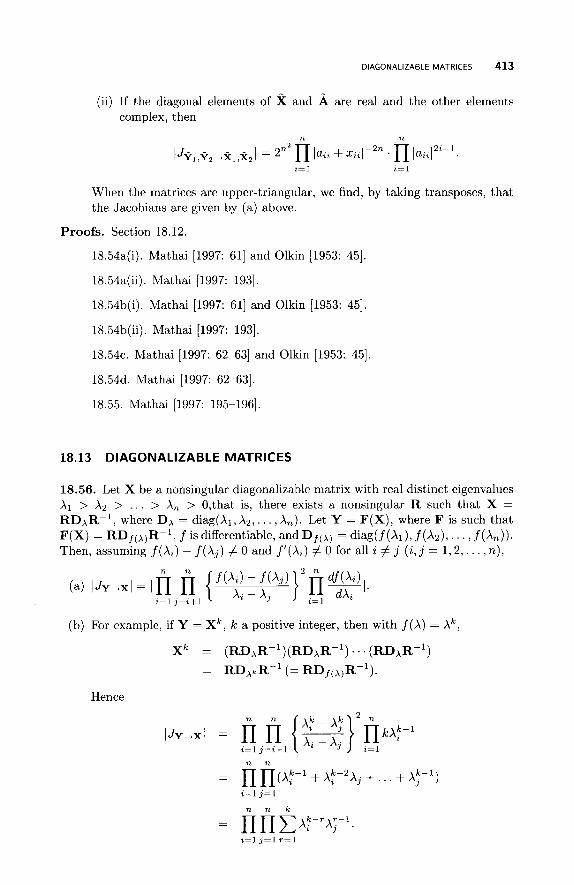
DIAGONALIZABLE MATRICES 413
(ii) If the diagonal elements of X and A are real and the other elements complex, then
n n
z = 1 i=l
When the matrices are upper-triangular, we find, by taking transposes, that the Jacobians are given by (a) above.
Proofs. Section 18.12.
18.54a(i). Mathai [1997: 611 and Olkin [1953: 451.
18.54a(ii). Mathai [1997: 1931.
18.54b(i). Mathai [1997: 611 and Olkin [1953: 451.
18.54b(ii). Mathai [1997: 1931.
18 .54~. Mathai [1997: 62-63] and Olkin [1953: 451.
18.54d. Mathai [1997: 62-63].
18.55. Mathai [1997: 195-1961,
18.13 D I AG 0 N A L I Z A B L E MATRICES
18.56. Let X be a nonsingular diagonalizable matrix with real distinct eigenvalues X1 > X2 > .. . > An > 0,that is, there exists a nonsingular R such that X = RDxR-', where Dx = diag(A1, A 2 , . . . ,An). Let Y = F(X), where F is such that F(X) = RDf(xlR-', f is differentiable, and Df(x) = diag(f(Al), f(A2), . . . , f ( A n ) ) . Then, assuming f ( X , ) - f ( A j ) # 0 and f ' (A , ) # 0 for all z # j ( z , j = 1 ,2 , . . . , n),
(b) For example, if Y = Xk, k a positive integer, then with f ( X ) = Ak,
xk = ( R D ~ R - ~ ) ( R D ~ R - ~ ) . . . ( R D ~ R - ~ )
= RD,,,R-~(= R D ~ ( ~ ) R - ~ ) .
Hence
n n
= rJ(A"-' + xf-2x.j + . . . + A;-')
414 JACOBIANS
The reader is also refered to (18.15a).
(c) In some applications, Y is a random matrix whose eigenvalues are distinct with probability 1. The Jacobian (Jx-yI is then given by IJy-xI-', but it is expressed in terms of the eigenvalues of X rather than Y, which is not so convenient in applications.
(d) If X is symmetric, then
Proofs. Section 18.13.
18.56a. Mathai [1997: 961 and Olkin and Sampson [1972: 267, lemma 91.
18.56b. Henderson and Searle [1979: 731).
18.56d. Mathai [1997: 961 and Olkin and Sampson [1972: 268, lemma 101.
18.14 PAIRS OF MATRICES
18.57. Let Y1 and Y2 be positive definite n x n matrices. If det(Y1 -XY2) = 0 has n distinct roots A1 > A2 > . . . > An > 0, there exists a unique matrix W = (wij), with wli > 0 (i = 1 , 2 , . . . , n) , such that Y1 = WDxW', Y2 = WW', and Dx = diag(A1,. . . , A n ) (cf. 16.51~). Then
n n
IJY~ ,YZ-W,DAI = 2n I(detW)n+2 n n (xi - x j ) l .
i=l j=i+l
18.58. Let X1 and X2 be positive definite.
(a) If Y1 = X,1/2X1X;1/2 and Y2 = X2, then Y1 and Y2 are positive definite and
I J Y ~ , Y ~ - x ~ , x ~ I = I detX21-(n+')/2.
(b) If Y1 = (XI + X2)-'/2X1(X1 + X Z ) - ' / ~ and Y2 = XI + X2, then Y1 and Y2 are positive definite and
I J Y ~ , Y ~ + x ~ , x ~ I = Idet(X1 + X2)l-(n+1)/2.
18.59. Let X1 and X2 be n x n positive definite matrices. If Y1 = XI and Y2 = X1 +X2, then Y1 and Y2 are positive definite and there exists a nonsingular V such that Y1 = VD,V', Y2 = VV', and D, = diag(&, . . . , &), where 1 > 41 > 49 > . . . > &, > 0 are the roots of det(X1 - +(XI + X2)) = 0. Then (cf. 18.57)
I J Y ~ , Y ~ - V , D + I = 2" I(det V)n+2 n n (4i - 4j)l. n n
i=l .j=i+l

PAIRS OF MATRICES 415
Proofs. Section 18.14.
18.57. Deemer and Olkin [1951: 3501.
18.58a. Mathai [1997: 1481.
18.58b. Mathai [1997: 1491 and Seber [1984: 5321.
18.59. Mathai [1997: 1511 and Olkin and Sampson [1972: 270, lemma 141.

This Page Intentionally Left Blank
CHAPTER 19
MATRIX LIMITS, SEQUENCES, AND SERIES
Asymptotic theory and large sample approximations play a key role in statistical distribution theory. In this chapter we apply some of theory of limits to vectors and matrices.
19.1 LIMITS
Definition 19.1. Let A(t) = ( u z 3 ( t ) ) . We say that limt-t,, A(t) = A if uz3( t ) ) -+
uz3 for all i , j . Of particular interest is the case when t = E and t o = 0, as in the following result.
19.1. Suppose A = ( u t 3 ) is nonsingular,
(a) The elements of A-l are continuous functions of the uz3.
(b) If lim,+o A(€) = A , then lim,,o[A(~)]-' = A-l.
(c) lim,,o(A - €I)-' = A-l .
(d) If A is m x n and B is n x m, both independent of E , then
A Matrix Handbook for Statisticians. By George A. F. Seber Copyright @ 2008 John Wiley & Sons, Inc.
417
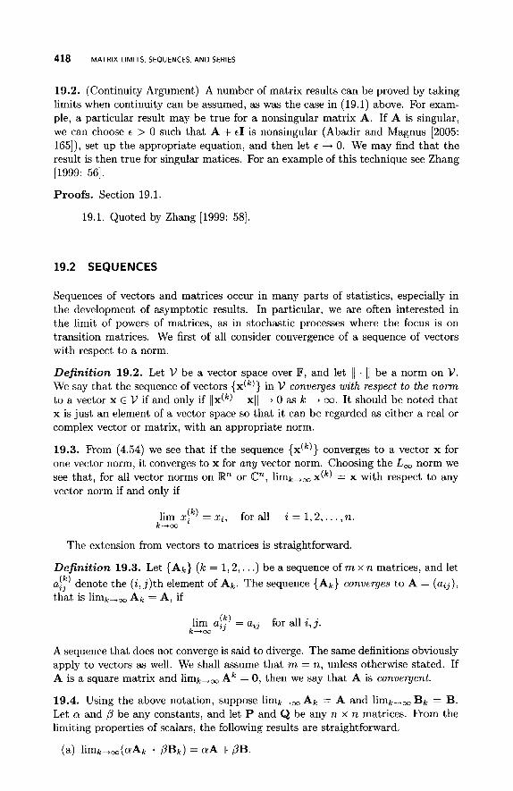
418 MATRIX LIMITS, SEQUENCES, AND SERIES
19.2. (Continuity Argument) A number of matrix results can be proved by taking limits when continuity can be assumed, as was the case in (19.1) above. For exam- ple, a particular result may be true for a nonsingular matrix A. If A is singular, we can choose E > 0 such that A + EI is nonsingular (Abadir and Magnus [2005: 165]), set up the appropriate equation, and then let E + 0. We may find that the result is then true for singular matices. For an example of this technique see Zhang [1999: 561.
Proofs. Section 19.1.
19.1. Quoted by Zhang [1999: 581.
19.2 SEQUENCES
Sequences of vectors and matrices occur in many parts of statistics, especially in the development of asymptotic results. In particular, we are often interested in the limit of powers of matrices, as in stochastic processes where the focus is on transition matrices. We first of all consider convergence of a sequence of vectors with respect to a norm.
Definition 19.2. Let V be a vector space over F, and let 1 1 . 11 be a norm on V . We say that the sequence of vectors {x")} in V converges with respect to the norm to a vector x E V if and only if I I x ( ~ ) - X I / -+ 0 as k -+ 00. It should be noted that x is just an element of a vector space so that it can be regarded as either a real or complex vector or matrix, with an appropriate norm.
19.3. From (4.54) we see that if the sequence {x(~)} converges to a vector x for one vector norm, it converges to x for any vector norm. Choosing the L , norm we see that, for all vector norms on R" or @", lirnk,,~(~) = x with respect to any vector norm if and only if
The extension from vectors to matrices is straightforward.
Definition 19.3. Let { A k } ( k = 1,2 , . . .) be a sequence of m x n matrices, and let a:;) denote the ( i , j ) th element of Ak. The sequence {Ak} converges to A = (a i j ) ,
that is limk,, Ak = A, if
A sequence that does not converge is said to diverge. The same definitions obviously apply to vectors as well. We shall assume that m = n, unless otherwise stated. If A is a square matrix and limk,, Ak = 0, then we say that A is convergent.
19.4. Using the above notation, suppose limk,, A k = A and limk,, B k = B. Let a and ,6 be any constants, and let P and Q be any n x n matrices. From the limiting properties of scalars, the following results are straightforward.
(a) hk+,((YAk + PBk) = d 4- PB.
SEQUENCES 419
(b) limk,, AkBk = A B .
(c) limk,, PAkQ = PAQ.
19.5. The sequence {Ak} converges if and only if the following hold.
(1) Each eigenvalue X of A satisfies either 1x1 < 1 or X = 1.
(2) When X = 1 occurs, the algebraic and geometric multiplicities of the eigen- value 1 are the same.
19.6. If there is a matrix norm 1 1 1 . 1 1 1 such that lllAlll < 1, then A is convergent.
19.7. A is convergent if and only if all the eigenvalues X are less than 1 in modulus (i.e., p(A) < 1, where p(A) is the spectral radius of A) .
19.8. If the eigenvalue 1 occurs with algebraic and geometric multiplicity t (i.e., is semisimple), and all other eigenvalues are less than 1 in modulus, then
lim A k = X(Y’X)-lY’,
where X and Y are the n x t matrices o f t linearly independent right, respectively, left eigenvectors associated with the eigenvalue 1.
19.9. Let A be n x n, let {Ak} ( k = I , 2, . . .) be a sequence of real n x n matrices, and let 1 1 1 . 1 I l p , z n be an matrix norm induced by the L, vector norm. If p = 1,2, or 00
(cf. 4.74), then
k-cc
(a) lirnk-, Ak = 0 if and Only if h k , , II(AkI(lp,zn = 0.
(b) limk,, Ak = A if and only if limk,, IllAk - AIIIp,tn = 0. If we use -
AllF, then this result also applies to m x n matrices; cf. Harville [1997: 4311.)
(c) If lirnk-, Ak = A , then limk,, ~ ~ ~ A k ~ ~ ~ p , ~ n = IIIAIIIp,tn. (The converse may not be true.)
19.10. The following result is useful in the context of limits. Suppose C is a square matrix and (I - C)-’ exists. If
19.11. If 1 1 1 . 1 1 1 is any matrix norm, then
where p is the spectral radius.
Proofs. Section 19.2.
19.3. Horn and Johnson [1985: 2731.
19.5. Hunter [1983a: 151-1521 and Meyer [2000a: 629-6301.
19.6. Harville [1997: 431-4321 and Horn and Johnson [1985: 2981
420 MATRIX LIMITS, SEQUENCES, AND SERIES
19.7. Graybill [1983: 98-99], Horn and Johnson [1985: 2981, and Meyer [2000a: 6171.
19.8. Hunter [1983a: 1531.
19.9. Graybill [1983: 96-97].
19.10. We use (19.14).
19.11. Meyer [2000a: 6191.
19.3 ASYMPTOTICALLY EQUIVALENT SEQUENCES
There are situations where an n x n matrix A is difficult t o work with, but a related matrix is easier to use that gives approximately the same result when n is large. This idea is made rigorous below.
Definition 19.4. Let {A(k)} and {B(k)} be two sequences of real matrices, where A(k) and B(k) are both k x k, and let lllAlllv denote a matrix norm. The two sequences of matrices are defined to be asymptotically equivalent if and only if they satisfy the following two conditions (Graybill [1983: 1011).
(1) IIIA(k)1112 5 c < 00, IIIB(k)(112 5 c < 00 for k = 1 , 2 , . . . , where c is a real
(2) limk,, k-1’2111(A(k) - B(k)lIl~ = 0.
number that does not depend on k .
19.12. Let {A(k)} and {B(k)} be two asymptotically equivalent sequences of k x k matrices.
(a) Then limk,, k-1/2111AklJJp = limk,oo k - 1 ~ 2 ~ ~ ~ B ~ ~ ~ ~ ~ .
(b) Suppose A&\ and BG; exist for each k = 1 ,2 , . . .. If llIA(k)(((2 5 c < 00 and lllBklll2 5 c < cc for k = 1,2, . . . , where c is a real number that does not depend on k , then {AG:} and {B&\} are asymptotically equivalent.
19.13. Let {A(k)), {B(k)}, {F(k)}r and { G ( k ) } be sequences of k x k matrices.
(a) If {A(k)) is asymptotically equivalent to {B(k)}, and {F(k)) is asymptoti- cally equivalent to {G(k) } , then {A(k)F(k)} is asymptotically equivalent to
{B(k)G(k)}.
(b) If, in (a,) {B(k)} is asymptotically equivalent to { C ( k ) } , then {A(k)} is asymp-
(c) If {A(k)B(k)} is asymptotically equivalent to { D ( k ) } , and IIIA&l)1112 5 c < m,
where c is a constant that does not depend on k, then {B(k)} is asymptotically equivalent t o {A,~,D(~,} .
totically equivalent to {C(,+)}.
Proofs. Section 19.3.
19.12. Graybill [1983: 101-1021.
19.13. Graybill [1983: 1021.
SERIES 421
19.4 SERIES
Definition 19.5. Let S k = Al+Aa+. . .+Ak, where the Ai a r e n x n . Theseries s k is said to converge to, or have sum, S if limk+W S k = S; we write S = CEl Ak. A series that does not converge is said to diverge. (In what follows we recall that p(A) is the spectral radius of A.)
19.14. If S k = I, + A + A' + . . . + Ak, then
s k = (I, - A)-'(I, - A"') = (I, - A"' )(In - A)-',
provided (I, - A)-' exists.
19.15. The following conditions are equivalent.
(1) (Newmann Series) I, + A + A' + . . . converges.
(2) 4-4) < 1.
(3) limk,, Ak = 0,that is, A is convergent.
Moreover, when one (and hence all) of these conditions are satisfied, then
(a) I, - A is nonsingular.
(b) I, + A + A' + . . . converges to (I, - A)-'.
19.16. Let A E V be the vector space of n x n matrices, and let 1 1 1 . 1 1 1 be any matrix norm defined on V .
If lllAlll < 1, then (I, - A)-' exists and is given by
m
(I, - A)-l = E A k . k=O
We can obtain another result by setting A = I, - B.
Suppose B E V and B is nonsingular. If F = B-'A, then the infinite series Bpl + FBP1+ F'B-' +. . . converges if and only if limk,m Fk = 0, in which case B - A is nonsingular and
03
(B - A ) - ~ = CF~BB-~. k=O
Replacing A by -A we get
W
(A + B)-' = (C(-B-'A)~)B-' k=O
If A is small, we have the approximation (A + B)-' M B-' - B-'AB-'.
If A is the matrix that is nonsingular, we interchange A and B.
If { a k } , IC = 0,1,. . . is a sequence of scalars, then CEO akAk converges if the series Cp=o l a k I . I I IAl I I of real numbers converges; Ao = I,.
422 MATRIX LIMITS, SEQUENCES, AND SERIES
(d) ~ ~ o c r k A k converges absolutely if cr=o la’klpk < m, where p = p(A) is the spectral radius of A.
Proofs. Section 19.4.
19.14. Consider (I, - A)Sk and S k ( 1 , - A ) and use Definition 19.3.
19.15. Graybill [1983: 1001, Hunter [1983a: 1541, and Meyer [2000a: 6181.
19.16a. We combine (19.6) with (19.15).
19.16b. Harville [1997: 4301.
19.16~. Rao and Rao [1998: 3661.
19.16d. Abadir and Magnus [2005: 2601.
19.5 MATRIX FUNCTIONS
Many functions f ( t ) , whether polynomial or nonpolynomial like exp(t), sin t , and so on, can be generalized to have a matrix argument. Horn and Johnson [1991: chapter 61 have a good discussion on the meaning of f (A) and associated properties. They also define a primary matrix function f (A) associated with the scalar-valued stem function f ( t ) using the Jordan canonical form of A, and their book should be consulted for details. We shall only consider some nonpolynomial functions. The following theorem is helpful in this respect.
19.17. Let f ( t ) be a scalar-valued function with power series representation f ( t ) =
a0 +alt+a2t2 +. . . that has a radius of convergence R > 0. If A is n x n and p(A) < R, where p(.) is the spectral radius, the matrix power series a0 + alA + a2A2 + . . . converges with respect t o every norm on the set of n x n matrices, and its sum is denoted by the primary matrix function f ( A ) .
19.18. Let A be n x n with eigenvalues xi, and suppose f (A) = cr=l C k X k and f ( A ) = cr=1 CkAk.
(a) Since A = RJoR-~, where J0 is the Jordan canonical form of A, we have f ( A ) = R f ( J 0 ) R - l .
(b) det f ( A ) = det R . det f(J0) . (det R)-’ = det(J0) = n:=, f ( A , ) .
(c) tracef(A) = t race(R-lRf(J0)) = trace(f(J0)) = cy=l f(&). See also (19.21).
A number of functions with power series expansions fall into the above category, the most common being the exponential function. In fact (I, + A)”, exp(A), logA, sinA, and cosA can all be defined as primary matrix functions. However, using the Jordan canonical form, we find that all functions f satisfying certain derivative conditions have the property that f ( A ) can be expressed as a polynomial in A (Meyer [2000a: 603-6071), For further details see Abadir and Magnus [2005: chapter 91 and Meyer [2000a: sections 7.3 and 7.91.
MATRIX EXPONENTIALS 423
Proofs. Section 19.5.
19.17. Horn and Johnson [1991: 412).
19.18b. The determinant is the product of its eigenvalues, which are the diagonal elements of the upper-triangular matrix Jo.
19.18~. As in (b), except that the trace is the sum of the eigenvalues.
19.6 MATRIX EXPONENTIALS
Matrix exponentials typically arise as solutions of differential equations (cf. Section 17.10).
Definition 19.6. If A is an n x n matrix, we define
t2 tr 2! r!
exp(At) = I, + t A + -A2 + . . . + -AT + . . . , -co < t < co.
This series converges absolutely for p(A) < 00 (by 19.16d).
19.19. Setting t = 1, we have the following.
(a) The eigenvalues of exp(A) are exp(&) (i = 1 ,2 , . . . , n), where the X i are the eigenvalues of A.
(b) If A is symmetric, then exp(A) is positive definite as each eigenvalue A, of A is real and exp(Xi) is positive.
(c) The matrix exp(A) is always nonsingular (as from (a) the eigenvalues are nonzero) and
[exp(A)]-l = exp(-A).
(d) exp(kA) = [exp(A)lk for k a positive or negative integer.
(e) [exp(A)]* = exp(A*). It then follows that exp(A) is Hermitian if A is Hermitian, and it is unitary if A is skew-Hermitian.
(f) Every n x n unitary matrix U can expressed as exp(iA), where A is some Hermitian n x n matrix. Note that iA is skew-Hermitian.
(g) If U is an n x n symmetric unitary matrix, there exists a real symmetric matrix A such that U = exp(iA).
(h) As the determinant of a matrix is the product of its eigenvalues, it follows from (a) that
since ni exp(Xi) = exp(Ci Xi).
det[exp(A)] = exp(traceA).
(i) If A is real skew-symmetric, then exp(A) is orthogonal and its determinant is 1.
424 MATRIX LIMITS, SEQUENCES, AND SERIES
(j) If A is skew-Hermitian, then C = exp(A) is unitary with I det CJ = 1.
19.20. Let A and B be n x n matrices.
(a) If A B = BA, then
exp(A + B ) = exp(A) exp(B) = exp(B) exp(A).
Although commutativity is a sufficient condition for the above to hold, it is not necessary.
(b) We can have exp(A)exp(B) = exp(B)exp(A), but AB # BA. For an example see Abadir and Magnus [2005: 2561.
(c) det[exp(A + B)] = det[exp(A)] det[exp(B)].
(d) (Lie Product Formula) limn-m [exp( p) exp( g)] This follows from (19.19g) above irrespective of whether (a) holds or not.
= exp(A + B).
19.21. Let A be an n x n diagonalizable matrix with eigenvalues Xi ; that is, there exists a nonsingular matrix R such that
A = RAR-’ = Rdiag(X1, X2,. . . ,Xn)RP1, ~k = R A ~ R R - ~
and exp(A) = Rdiag(exl , . . . , eXn)R-’ = ReARP1, say.
(This method avoids using a power series expansion, and it can be generalized to any function f ( z ) of a diagonalizable matrix by defining f (A) = diag(f(Xl), f(&), . . . , f(X,)) and setting f ( A ) = Rf(A)R-’.) For nondiagonalizable matrices, we can replace A by its Jordan form Jo and use (19.18).
19.22. For general t :
(a) The matrix exp(At) is nonsingular for all finite t . Noting that its eigenvalues are exp(tXi), we have from (19.19g),
det (exp(At) = exp(ttraceA), -m < t < 00.
(b) Using power series expansions, exp(At1) exp(At2) = exp[A(tl + t2)] for all tl and t2.
(c) [exp(At)]-’ = exp(-At).
(d) If “8” is the Kronecker product, we have from (11.9):
(i) exp(I,, 8 At) = I, @I exp(At).
(ii) exp(At 8 Im) = exp(At) 8 I,.
These results hold for any primary matrix function f(.) and not just for exp(.).
(e) exp(At) exp(Bt) = exp[(A+B)t] for all finite t E R if and only if AB = BA.
19.23. (Inequalities)
MATRIX EXPONENTIALS 425
(a) Let A be any n x R matrix. For any matrix norm 1 1 1 . 1 1 1 ,
I l l exp(A)III I exP(lllAIl0.
(b) If A and B are n x n Hermitian matrices, then
II exp(A + B)IIui I II exp(A) exP(B)Ilui,
for any unitarily invariant norm 1 1 . llUi .
19.24. Let f be a continuous function from the space of n x n complex matrices to C with the following properties.
(1) f(XY) = f (YX) for all X and Y.
(2) I(f(X2k)l 5 f([XX*Ik) for all X and for all k = 1,2, . . ..
Then:
(a) f ( X Y ) 2 0 for all Hermitian non-negative definite X and Y. In particular,
f(exp(A)) 2 0
for all Hermitian A.
(b) If(exp(A))l I f(%eA) for all A.
(c) If(exp(A + B))I I f(!Re(A + B)) I f (%eA)f(ReB) for all A , B.
(d) 0 I f(exp(A + B) 5 f(exp(A) exp(B)) for all Hermitian A, B.
Here %e means the “real part of.” Note that (a) and (d) hold when f is the trace or the determinant. The above inequalities arise in statistical mechanics, population biology, and quantum mechanics.
Proofs. Section 19.6.
19.19a. Follows from the fact that A k x = Akx for all k = 1 ,2 , . . ., and for some x. See also Meyer [2000a: : 5251
19.19~. Horn and Johnson [1991: 4351.
19.19d. Abadir and Magnus [2005: 2621 and Horn and Johnson [1991: 4351.
19.19e. Quoted by Horn and Johnson [1991: 439, exercise 91.
19.19f. Quoted by Horn and Johnson [1991: 440, exercise 101.
19.19i. Abadir and Magnus [2005: 2631.
19.19j. Abadir and Magnus [2005: 2641.
19.20a. Abadir and Magnus [2005: 252-531 and Horn and Johnson [1991: 4351.
19.20b. Quoted by Horn and Johnson [1991: 442, exercise 221.

426 MATRIX LIMITS, SEQUENCES, AND SERIES
19.20~. Bhatia [1997: 2541 and Horn and Johnson [1997: 4961.
19.21. Abadir and Magnus [2005: 2601 and Meyer [2000a: 525, 6011.
19.22~. Use (e) to verify that exp(-At) is the inverse.
19.22d. Quoted by Horn and Johnson [1991: 440, exercise 131.
19.22e. Abadir and Magnus [2005: 2521.
19.23a. Horn and Johnson [1991: 501, equation (6.5.25)].
19.23b. Horn and Johnson [1991: 4991.
19.24. Horn and Johnson [1991: 4971.
CHAPTER 20
RANDOM VECTORS
20.1 NOTATION
In this chapter we do not use the convention that random variables have capital letters because of the problem of distinguishing between a random matrix and its observed value in the next chapter. As a rough rule, we generally reserve the latter part of the alphabet, u, u, . . . , z for random vectors and the rest of the alphabet for constants, including matrices of constants.
20.2 VARIANCES AND COVARIANCES
Definition 20.1. I f x = ( x i ) is a vector of random variables, then we define E(x) = (E(lci)), the vector of expected values.
20.1. For conformable vectors and matrices, E(Ax + b) = AE(x) + b.
20.2. Let S be a convex subset of R” and x an n x 1 random vector with finite E(x). If pr(x E S ) = 1 then E(x) E S.
Definition 20.2. If x and y are vectors of random variables, we define the matrix with ( i , j ) t h elements cov(zi,yj) to be cov(x,y), the covariance matrix of x and y. When x = y , we define var(x) = cov(x,x) to be the variance matrix of x. (The terms variance-covariance matrix, covariance matrix and dispersion matrix
A Matrix Handbook for Statisticians. By George A. F. Seber Copyright @ 2008 John Wiley & Sons, Inc.
427
428 RANDOM VECTORS
are also used in the literature for var(x).) In the following, we recall that A implies that A - B is non-negative definite.
20.3. Let var(x) = C. Since, by (20.6b), 0 5 var(a’x) = a’Ca, we have that C is non-negative definite. It is nonsingular (i.e., positive definite) if and only if there do not exist constants a (# 0) and b such that a’x = b (i.e, var(a’x) = 0).
20.4. If E(x) = p and var(x) = C, then x - p E C(C) or equivalently x E C(p, C), with probability 1.
20.5. Let E(x) = px and E(y) = py.
B
( 4
cov(x - a, y - b) = cov(x, y) = E “ x - P d Y - P Y Y I
= E(xY’) - pxp;.
(b) The above result also holds if x = y so that:
(i) var(x - a) = var(x).
(ii) var(x) = E(xx’) - pxpL.
20.6. The following results are extremely useful.
(a) cov(Ax, By) = Acov(x, y)B’.
(b) From (a), var(Ax) = Avar(x)A’.
(c) var(y - Ax) = var(y) - Acov(x, y) - cov(y, x)A’ + Avar(x)A’.
20.7. If x and y are random vectors with respective means px and py , then E((y - Ax - a)(y - Ax - a)’] = var(y - Ax) + (py - Apx - a ) ( p y - Apx -a)’.
20.8. If a, b, c, and d are constants, then
cov(ax + by, c u + dv) = accov(x, u) + ad cov(x, v) + bccov(y, u) + bdcov(y, v).
In particular, var(u + v) = var(u) + cov(u, v) + [cov(u, v)]’ + var(v)
20.9. (Partitioned Vector) Let z = (x’ ,~’)’ be a random vector with mean pz = (pL,pb)‘, where x is m x 1 and y is p x 1. Then:
var(x) cov(x, y) (a) var(z) = Cz2 =
where Cyz = Cky.
(b) C(xZy) 2 C(Czz) and C(Eyz) C C(Cyy)
(c) If E(x) = 0, then cov(y -Ax, x) = 0 if and only if Ax = Bx with probability 1, where B = CYzC;, and C;, is any weak inverse of C,, (i.e., C,,C;,C,, =
Em).
VARIANCES AND COVARIANCES 429
(d) Using (20.8) and (c),
var(y - Ax) =
=
t var(y - Bx).
var[(y - Bx) + (B - A)x)
var(y - Bx) + var[(B - A)x]
for all A.
(e) By (20.6b) we have var(EyzE&x) = var(Bx) = EyzE;zEzY. This matrix and the generalized Schur complement Eyy.z = Eyy - EyzE;zEzy are invariant with respect to the choice of weak inverse ELz (by (14.8) and (20.9b)).
( f ) var(y - Bx) = Eyy.z (= var(y - py - EyzE&(x - p x ) ) , by (20.5b(i)).
(g) (Best Linear Predictor) From (20.7) and (d),
E[(y - A x - a) (y - Ax - a)’] k var(y - Ax)
?
for all conformable A and a, where yx = py + EzYELz(x - p x ) is called the best linear predictor as it minimizes the left-hand side of the above expression, the so-called mean squared prediction error matrix.
E[(Y - %)(Y - FX)’] = Eyy.”
Proofs. Section 20.2.
20.2. Schott [2005: 3771.
20.3. Seber and Lee [2003: 81.
20.4. Rao [1973a: 5221 and Sengupta and Jammalamadaka [2003: 561.
20.6a. Seber and Lee [2003: 71.
20.6~. Expand cov(y - Ax, y - Ax).
20.7. We use (20.5b(i)) with x replaced by y - Ax, and then use (20.5b(ii)) with x replaced by y - A x - a.
20.8. Seber and Lee [2003: 71.
20.9b. Sengupta and Jammalamadaka [2003: 56, with the roles of x and y interchanged].
20.9~. Sengupta and Jammalamadaka [2003: 571
20.9d. Use (20.9~) to prove that the covariance term is zero.
20.9e. var(Bx) = BE,,B’ = EyzE&Ezz(E;z)’Ezy = Eyz(E.&EzzE- where (E&)’ = E&l), say, for some weak inverse E&l) of Ezz, as Ezz is sym-
metric. Then C = E;zEzzE~z~l) is a weak inverse of Ezz as EzzCEzz = Ezz.
20.9f. Using (c) and B = EyzE;z, we obtain
)Ezy, 4 1 )
cov(y - Bx, y - Bx) = cov(y - Bx, y ) = var(y) - Bcov(x, y) = E:yy.z.
20.9g. E[(y - A x - a ) ( y - A x - a)’] k var(y - Ax), by (20.7), and var(y - Ax) k var(y - Bx), from (f) .
430 RANDOM VECTORS
20.3 CORRELATIONS
20.3.1 Population Correlations
Definition 20.3. If x and y are random variables, then their population correla- tion coeficient is defined to be p(x , y) = cov(x, y ) / [ ~ a r ( z ) v a r ( y ) ] ~ / ~ ( = ozy/(ozoy),
say).
20.10. p = p(x, y) has the following well-known properties.
(a) -1 5 p 5 +1.
(b) p2 = 1 if and only if x and y are linearly related. If p = tl, then y - py = z ( x - pz).
if p = -1, then y - py = - z ( x - pz).
(c) p(az, by) = sign(ab) lab1 P ( X l Y) .
Definition 20.4. Suppose x has variance matrix I: = (aij). If corr(x) = ( p z j ) , where pij = ~ij/(oiiojj)’/~, then corr(x) is called the populat-7n correlation ma t r i x of x.
20.11. Let C = corr(x) = (pij) be an n x n correlation matrix.
(a) C = D,1/21:D,’/2, where D, is a diagonal matrix with positive diagonal elements u = diag(al1, ~ 2 2 , . . . , onn).
(b) C is non-negative definite (as I: is).
(c) pii = 1 and Jpijl < 1 (for all i , j , j # i ) .
(d) The largest eigenvalue of C is less than n.
(e) 0 < det C 5 1.
(f) A well-known correlation matrix is of the form C = (1 - p)I, + pJ,, where J, is an n x n matrix with all its elements equal to 1. For C to be positive definite we must have -l/(n - 1) < p < 1. For further details about this matrix see (15.18a).
Definition 20.5. Let x be a d-dimensional random vector with E(x) = p and var(x) = I:, where I: is positive definite. Consider the partitions
where x2 = ( 2 2 , . . . ,xd)’, p2 = (pz , . . . ,pd)’ and &2 is (d - 1) x (d - 1). Here var(x1) = ollr u 1 2 is the vector of covariances betweem x1 and each of the variables in x2, and var(x2) = X22. The (population) multiple correlation coeficient between x1 and x2, denoted by ~ 1 . 2 3 . . .d l is the maximum correlation between x1 and any linear function a’x2 of 22,. . . , xd. Thus
CORRELATIONS 431
Also, R2 is sometimes called the (population) coef ic ient of multiple determinat ion, and R is the positive square root (Muirhead [1982: section 5.21 and Anderson [2003: section 2.51).
20.12. R has the following properties.
(a) R = ( ~ : ~ ~ : 2 2 0 1 2 / 0 1 1 ) ~ / ~
(b) 0 5 R 5 1.
(c) If d1 is the first diagonal element of X-’, then, from (14.11),
U 1 l = (011 - “ ;2X&712)-1
and 1 - R2 = l/(u1’u11).
(d) When x has a nonsingular multivariate normal distribution N d ( P , X) we have from (20.23f) that
E(xi I x 2 ) = pi + &X:,-,’(xz - P Z )
and var(x1 I x 2 ) = u l l . 2 3 . . . d = u11 - a ~ , ~ ~ ~ a 1 2
Then:
(i) 1 - R2 = 011.23 . . .d/ u l l .
(ii) 011.23.. .d 5 u11.
(iii) R is the correlation beween x1 and E(x1 I x 2 ) .
(e) When d = 2, R = Ip1.21 = Ip(~1,xz)l
Definition 20.6. The previous Definition 20.5 can be readily generalized. Let x be a &dimensional random vector with E(x) = ,u and positive definite variance matrix X. Consider the partitions
where XI is k x 1, x 2 is (d - k ) x 1, and so on, and let xi be a variable in x1 (i = 1,2, . . . , k ) . The (population) multiple correlation coefficient between xi and the variables x k + l , . . . , x d in x 2 , denoted by Ri . k + l , k + 2 ,.._, d, is the maximum correlation between x, and any linear function a’xz of x k + 1 , . . . ,xd. Note that R 1 . 2 ,..., d = R.
Definition 20.7. Using the notation of the previous definition, let X l l . 2 = -
(cf. 20.23f). We define the (population) partial correlation coef ic ient pi j . k+l , . . . ,d to be the correlation coefficient between xi and xj, components of X I , in the condi- tional distribution of x1 given x 2 , that is,
X 1 2 X ; i X 2 1 ( = (aij .k+l , . . . ,d ) , say). Given x - N d ( k E), then X11.2 = var(x1 I x 2 )
This is the correlation beween xi and xJ holding x2 fixed.
432 RANDOM VECTORS
Proofs. Section 20.3.1.
20.11d. The eigenvalues A, of C are non-negative and C, A, = trace C = n.
20.11e. Follows from (n, exceed the arithmetic mean) and det C = n, Xi .
20.12. Muirhead [1982: section 5.21
20.13. Anderson [2003: 38-41]; see also Muirhead [1982: 1941.
5 = 1 (a the geometric mean does not
20.3.2 Sample Correlations
Definition 20.8. If x = (2 , ) and y = (yi) are n x 1 vectors representing univariate random samples of size n, then their sample correlation coeficient is defined to be
20.14. T = r(x, y) has the following properties.
(a) r2 5 1. When r2 = I, there is a linear relation between the yi and the zi as in (20.10b), but with parameters replaced by their estimates.
(b) ax, by) = sign(ab) lab1 r(x, y).
Definition 20.9. Let XI, x 2 , . . . , x, be a random sample from a d-dimensional distribution with mean p and positive definite variance matrix X, and let S = ( S , ~ )
be the sample covariance matrix given by S = C7=l(xz - X)(x, - X ) ' / ( n - 1). Let rt3 = S ~ ~ / ( S , , S ~ ~ ) ~ / ~ , where r,, = 1 for i = 1 , 2 , . . . , d. Then R = ( T ~ ~ ) is called the sample correlatzon matrzx. It does not matter if we use n instead of (n - l), that
CORRELATIONS 433
is, use 2, the maximum likelihood estimate of X under normality, instead of S as (n - 1) cancels out of R. Note that S is a random matrix so that it is considered again in the next chapter.
20.15. We now introduce an important device that allows the properties of pop- ulation parameters to be carried over directly to their sample estimates. Consider the discrete random variable y with probability function
1 n
p r ( y = x i ) = - , i = 1 , 2 , . . . , n.
Then
n 1 - 1 1 - E(y) = Exz- = x and var(y) = x(xi - x)(xi - 5) - = X.
n z=1 i = l
We can therefore “translate” sample properties into population properties using an appropriate discrete population.
Definition 20.10. Using the notation of the previous definition, consider the partition
The sample multiple correlation coefficient between x 1 and ~ 2 ~ x 3 , . . . , xd is defined to be
R = ( s ~ , S ~ ~ s l ~ / s 1 1 ) 1 / 2 .
Under normality, R is the maximum likelihood estimate of R, the population mul- tiple correlation. For further details see Anderson [2003: section 4.41.
Sample versions of the other correlations and partial_correlations can be defined in a similar manner. One simply replaces X by S or X in the population defini- tions. For example, replacing X by S in Definition 20.7, we have the sample partial
For further details see Anderson [2003: section 4.31.
20.16. Using the method of (20.15), all the results and optimal properties for population parameters hold for the sample equivalents. For example, from (20.13b),
rz . k + l , k + 2 , . . . , d = ( s ~ s ~ ~ ~ z / s t z ) 1/2 .
Proofs. Section 20.3.2.
20.14a. Proved using the Cauchy-Schwarz inequality or using (20.15).
20.16. Muirhead [1982: 1881.
434 RANDOM VECTORS
20.4 QUADRATICS
20.17. Let x be an d-dimensional random vector with E(x) = p and var(x) = E, a non-negative definite matrix of rank T 5 d. Let A be a real d x d symmetric matrix, and let E = BB’ (cf. 10.10), where B is d x T and B’AB # 0. Then:
(a) With a suitable transformation of the form x = B P z we find that
i=l i=l r
bi b:
xi = C X i ( z i + - ) 2 + ( a - - C ) , X i f O , i = 1 , 2 , . . . , T
i=l i=l
i=l
where b’ = ( b l , b2 , . . . , b,) = p’ABP, z = (z1,z2,. . . , z r ) ’ , E(z) = 0, var(z) = I,, P’B’ABP = diag(X1, X 2 , . . . , X r ) , the X i are the eigenvalues of B’AB (i.e., of EA), P is r x T and orthogonal (i.e., PP’ = I?), and a = p’Ap.
(b) If E is positive definite, we can choose B to be triangular (Cholesky decom- position) or Ell2 (cf. 10.32). In the latter case, we find that
i=l
where the X i are the eigenvalues of E1/2AX’/2 (i.e., of XA), E(u) = 0, var(u) = Id, c’ = (clrc2,. . . , cd ) = (P’X-1/2p)’, and PP’ = I d .
20.18. Let x have mean p and non-negative definite variance matrix X, and let Q = E[(x - a)’A(x - a)] (= E[trace{(x - a)’A(x - a)}]).
(a) Using (20.7),
E(Q) = trace{AE[(x - a) (x - a)’]} = trace(AX) + ( p - a)’A(p - a)’.
(b) If X = 021, we have the useful rule E(Q) = o2 traceA + Q x + ~ ( x ) .
20.19. Let x be a d x 1 random vector with mean p, variance matrix X, and finite fourth moments, so that E(xx’) and E(xx’ 8 xx’) exist, where “8” refers to the Kronecker product. If A and B are real symmetric d x d matrices, then
COV(X’AX, x’Bx) = trace{ ( A @ B)E(xx’ 8 xx’)}
-{trace(AE) + p’Ap}{trace(BX) + p’Bp}.
20.20. Let x be a random vector with elements 21, x2,. . . , 5, distributed as in- dependent random variables with means & , &, . . .,&, common variance p2, and common third and fourth moments about their means, p3 and p4, respectively (i.e., pr = E[(zi - &).I). Let A be any symmetric n x n matrix, and let a = diagA be the column vector of the diagonal elements of A.
MULTIVARIATE NORMAL DISTRIBUTION 435
(a) We have
var(x’Ax) = (p4 - 3p;)a’a + 21-1; trace(A2) + 4p2fl’A2f3 + 4p38‘Aa.
(b) If the xi are each normally distributed as N(O,a’), then 1-13 = 0, 1-14 = 3,4, 1-12 = a’, and
If B is also a symmetric n x n matrix, then
var(x’Ax) = 2a4 trace(A2).
COV(X’AX, x’Bx) = 2a2 trace(AB).
These results are generalized in (20.25).
(c) Let 7 2 = (1-14 - 3,4)/p: be the common kurtosis, and let Pi (i = 1,2) be sym- metric idempotent matrices with pi = diag(Pi), r ankp i = fi (= trace Pi), and P I P 2 = 0. If Pi0 = 0, then from (a) we have:
(i) var(y’Piy) = h4(fi + +yzpI,pi).
(ii) C O V ( Y ’ ~ ~ Y , Y ’ ~ ~ Y ) = a472p’,p2.
This result is useful in examining the robustness of the F-test for a linear hypothesis and a linear model.
Proofs. Section 20.4.
20.17a. Mathai and Provost [1992: 361.
20.17b. Mathai and Provost [1992: 28-29].
20.18. Schott [2005: 4141 and Seber and Lee [2003: 91.
20.19. Schott [2005: 4141.
20.20~~. Quoted by Atiqullah [1962] and derived in Seber and Lee [2003: 10- 111.
20.20b. Seber and Lee [2003: 161.
20.20~. Atiqullah [1962] and Seber and Lee [2003: 236-2371. Here (ii) is obtained from ;{var[(y’(Pl + P,)y] - xi var(y’Piy)}.
20.5 MU LT I VA R I AT E N 0 R M A L D I STR I B U TI 0 N
20.5.1 Definition and Properties
Definition 20.11. Let x be a d x 1 random vector with mean p and variance matrix E, which is positive definite. Then x is said to have a (nonsingular) multivariate normal (or multinormal) distribution if its probability density function is given by
f(x) = f ( X l 1 X 2 , ’ ’ 1 4
= ( 2 ~ ) - ~ / ~ ( d e t E)-”’exp{~(x - P)’X-’/~(X - p ) }
( - -oo<z~<-oo, i = 1 , 2 , . . . , d) .
436 RANDOM VECTORS
We write x N N d ( p , E). When d = 1, we replace N1 by N , the univariate normal distribution. Note that x N N d ( 0 , I d ) if and only if the zi are independently distributed as N ( 0 , l ) . If x - N d ( p , E), then y = E-’l2(x - p ) - N d ( 0 , I d ) . Sampling from a normal distribution is discussed in Section 21.3.
If I: is positive semi-definite (i.e., singular), then the probability distribution still exists, but not the density function. However, we can extend our definition to include the so-called singular multivariate normal distribution using one of the two following equivalent definitions, which includes both the nonsingular and singular cases.
1. The random vector x is multivariate normal if and only if y = a’X is univariate normal for all a . If y = b we define y to be N(b, 0).
2. A random d x 1 vector x with mean p and variance matrix I: has a multivariate normal distribution if it has the same distribution as Az + p, where A is any d x m matrix satisfying E = AA’, and z N Nm(O,Im) .
The singular normal distribution occurs in many places in statistics, for example the distribution of residuals from linear models (Seber and Lee [2003]) and the distribution of the estimated cell proportions from sample survey data (Rao and Scott [1984]). For a general reference on the multivariate normal see Tong [1990].
20.21. Adopting the notation of Definition 20.11, suppose that X is singular of rank r (i.e., positive semi-definite). Then, from (20.4), x - p E C(E) and we can express I: = RR’, where R is d x T of rank r (cf. 10.10). Hence if P x is the orthogonal projector onto C(I:) (cf. 2.49d), we have, for ( Id - Pc)(x - p ) = 0, the density function
f (x) = (2~)~/~[det(R’R)]-~/~exp[-+(x - p)X-(x - p) ] ,
and 0 otherwise. Here E- is a weak inverse of E.
20.22. (A Useful Integral) If A and B are symmetric n x n matrices and B is positive definite, then using the multivariate normal density function we have
+W f W
(x’Ax + a’x + ao) exp[-(x’Bx + b‘x + bo)] d z l . . . dx,
- - 17rn12 2 IB I -1/2 exp( a b’B-lb - bo) 1, ’ . ’ L
x[trace(AB-’) - a’B-lb + ib’B-lAB-lb + 2ao].
20.23. Let x - Nd(p , I:), where the distribution may be singular or nonsingular.
(a) The moment generating function of x is E[exp(t’x)] = exp(t’p+ it’I:t). This uniquely determines the (nonsingular) distribution when C is positive definite.
(b) If C is m x d, then Cx - Nm(Cp, CEC’). The distribution is nonsingular if E is positive definite and C has rank m.
(c) Any subset of a multivariate normal distribution is multivariate normal.
(d) If the covariance of any two vectors that contain disjoint subsets of x is zero, then the two vectors are statistically independent.
MULTIVARIATE NORMAL DISTRIBUTION 437
(e) If cov(Ax, Bx) = 0, then A x and Bx are statistically independent.
(f) Suppose E is positive definite, and let
where x, and p, are d, x 1, Et, is d, x d, (i = 1,2), and dl +d2 = d. We then have the following conditional distribution
x2 I x1 - Ndz(p2.1 ,E22.1)r
where p 2 . 1 = p 2 + E21EF:(xl - p1) and E22.1 = E22 - E21Ey/E12. Note that E22.1 is the Schur complement of El1 in E, and it is frequently expressed in the form (X/E11) (cf. Section 14.1).
(g) The result ( f ) still holds if E is singular and we replace Er: by ETl, any weak inverse of El 1 .
20.24. (Moments) If x N N d ( 0 , E), where E is positive definite, and P d = ;(Id2 + I(d,d)) (= N d , the symmetrizer of (11.29h-i)), then:
(a) E(x 8 x) = vec E.
(b) E(xx’ 8 xx’) = 2Pd(E 8 E) + (vec E)(vec E)’.
If just one of any of the x’s is replaced by a constant vector, then the answer is 0.
(c) var(x 8 x) = 2Pd(E 8 E).
(d) Suppose x N N d ( p , E) and E is positive definite.
(i) E(x @ x) = E(z 8 z) + p @ p = vecX + ( p 8 p ) , where z = x - p.
(ii) var(x 8 x) = 2Pd(X 8 E + E 8 pp‘ + pp’ 8 X).
(e) Higher moments are given by Graybill [1983: section 10.91 for the case x N
N d ( 0 , I d ) .
Proofs. Section 20.5.1.
20.21. Sengupta and Jammalamadaka [2003: 581.
20.22. Graybill [1983: 3421 and Harville [1997: 3221.
20.23. Anderson [2003: chapter 21 and Seber and Lee [2003: chapter 21. For ( f ) see Schott [2005: 260-2611 and Seber and Lee [2003: 25-26], and for (g) see Sengupta and Jammalamadaka [2003: 591.
20.24a-c. Schott [2005: 4161.
20.24d(i). Schott [2005: 4161.
20.24d(ii). Abadir and Magnus (2005: 3101.
438 RANDOM VECTORS
20.5.2 Quadratics in Normal Variables
20.25. Let x - Nd(p, X), where E is positive definite.
(a) We have (x - p)’X:-l(x - p ) N xz and x’X-’x - x;(S), the noncentral chi-squared distribution with noncentrality parameter 6 = p’E-’p.
(b) Using the notation of (20.23f), we have the following:
(i) Q1 = (XI - pl)’Xcf(xl - p1) - xzl (by 20.23~ and (a) above).
(ii) Let Q2 = (x - p)’X-l(x - p ) - (XI - pl)’X;f(xl - pl ) . Then, from (20.23f), x2 I x1 N Ndz(p2.1,E22.1) and, conditional on X I ,
2 Q2 1 ( ~ 2 - P Z . I ) ’ E ~ ; ~ ( X ~ - ~ 2 . 1 ) N x d 2 .
Since this distribution is not a function of xl, it is also the unconditional distribution; (iii) below holds for the same reason.
(iii) Q1 and Qz are statistically independent.
(c) Let A and B be d x d matrices.
(9
E(x’Ax. x’Bx) = trace(AX) trace(BX) + 2 trace(AEBX)
+ trace(AX)p’Bp + trace(BE)p’Ap
+4p’AXBp + (p’Ap)(p’Bp).
(ii) COV(X’AX,X’BX) = 2 trace(AEBX) + 4p’AXBp.
(iii) Setting A = B in (ii), we have
var(x’Ax) = 2 t r a ~ e [ ( A X ) ~ ] + 4p’AEAp.
(d) Let x - N d ( O , I d ) , and let A, B, and C be all d x d symmetric matrices.
(i)
E(X’AX. x / ~ x . x’cx) = trace A trace B trace C + 2 trace A trace(BC)
+2 trace B trace(AC) + 2 trace C trace(AB)
+ 8 trace(ABC).
(ii) If x N Nd(0, X), we replace A, B, and C in the right-hand side of (i) by AX, BE, and CE, respectively.
(e) If x - N d ( 0 , X), then:
6) COV[ (x’Ax)~, (x’Bx)]
= 4 trace(AX) trace(AXBX) + 8 t r a ~ e [ ( A E ) ~ B X l .
MULTIVARIATE NORMAL DISTRIBUTION 439
(ii)
E [ (x’ Ax) ’1 = [trace(AE)]’ + 6 trace(AE) trace[(AE)’] + 8 trace[(AE)’].
( f ) (Moment Generating Function) If Q = x’Ax + a’x + d, where A is real and symmetric, then the moment generating function (m.g.f.) of Q is
i= 1
d
where T’X1/’AE112T = diag(A1,. . . ,Ad),
T is orthogonal, and
c = (c1, . . . , cd)’ = T’(E1/’a + 2E1/’Ap).
Note that
d
n(1 - 2tAi)-1/2 = [det(Id - 2tE1/2AE1/2)]-1/2 = [det(Id - 2tAE)]-’/’.
The m.g.f. can be used to obtain moments of the quadratic form-for example, (c)(iii). Thus if QO = x’Ax we have:
(i) E(Q0) = trace(AE) + p’Ap.
(ii) E[(Qo)’] = 2 trace[(AE)’] + 4p’(AE)Ap + {trace(AE) + p’Ap}’.
(iii)
i=l
E [ ( Q o ) ~ ] = 8{trace[(AE)’] + 3p’(AE)’Ap}
+ 6{t ra~e[ (AE)~] + 2p’AEp}{trace(AE) + p‘Ap}
+{trace(AE) + p‘Ap}’.
General expressions for E(QZ;) and E(QT) are given by Mathai and Provost [1992: 53-54], who also give formulae for E(Qch), where h > 0 and can be a fraction (Mathai and Provost [1992: 56-59]).
440 RANDOM VECTORS
20.26. Let x have the singular normal distribution N d ( p , C ) , where C is non- negative definite of rank T (T < d).
(a) x’C+x - x;(b), the noncentral chi-squared distribution with noncentrality parameter 6 = p’Cp. Here C+ is the Moore-Penrose inverse of C.
(b) (Moment Generating Function) Let C = BB’ (cf. 10.10), where B is d x T
of rank T and B’AB # 0. If A is a d x d real symmetric matrix, then the moment generating functiom (m.g.f.) of Q = x’Ax + a’x + d is
M Q ( ~ ) = [det(I, - 2tB’AB)]-1/2 exp{t(p’Ap + a’p + d )
+$(B’a + 2B’Ap)’(Id - 2tB’AB)-’(B’a + 2B’Ap)).
An alternative expression in terms of eigenvalues is given by Mathai and Provost [1992: 46-47]. Positive, negative, and fractional moments of QO = x’Ax are given by Mathai and Provost [1992: 54-55, 61-65].
The characteristic function of Q is obtained from the m.g.f. by replacing t by i t , where i = n.
20.27. Let Qi = x’Aix + a:x + di, where Ai is a real d x d symmetric matrix ( i = 1 , 2 ) , and suppose x - N&, C).
(a) If C is positive definite, then the joint moment generating function (m.g.f.) of Q1 and Q 2 is
M ~ ~ , ~ ~ ( t l , t a ) = [det(I, - 2tlA1E - 2t2A~E:)]-’/~
x exp{-$(p’E-lp - 2tldl - 2t2d2)
xC-l(tlCal+ t2~a2 + p ) } .
+2(tlCal 1 + t2Ea2 + p)’ (Id - 2tlAlC - 2tZAzC)-’
(b) If E is non-negative definite and C = BB’ (cf. 10.10), where B is d x T of rank T (T < d) , then the joint m.g.f. of Q1 and Q 2 is
M ~ ~ , ~ ~ ( t l , t 2 ) = [det(I, - 2tlB’AlB - 2t2B’A2B)]-’/’
x exp(tl(p’A1p + a;p + dl) + t2(p’A2p + alp + d2)
+;@(I, - 2tlB’AB - 2t2B’AB)P},
where
p = (I, - 2tlB’AiB - 2tzB’A2B)-l
x(tlB’a1 + 2t2B’Alp + tzB’a2 + 2t2BtA2p).
Note that (a) follows from (b) by setting B = B’ = (cf. 10.32). We can obtain various special cases, for example: (i) if we set ai = 0 and di = 0 for i = 1 , 2 , and p = 0, we get the joint m.g.f. of x’A1x and x‘A~x, or (ii) if we set A2 = 0 we get the joint m.g.f. for a quadratic and a linear form.
In (a) and (b), the joint characteristic function is obtained by replacing tl and t~ by it1 and i t 2 , respectively where i = &f.
The above results were proved by Mathai and Provost [1992: 66, section 3.2~1 and extended to more than two quadratics. They can also be used to obtain various
MULTIVARIATE NORMAL DISTRIBUTION 441
product moments, for example if E is positive definite or non-negative definite we have
( i ) cov(x’Ax, a’x) = 2p’AEa.
(ii) cov(x’Alx, x’A~x) = 2trace(AlEAzE) + p‘AlCA2p.
The m.g.f.s can also be used to obtain cumulants. The reader is referred to Mathai and Provost [1992: sections 3.2d and 3.31 for further details.
20.28. (Distribution of a Quadratic) If x N Nd(p, C), where C is positive definite, and A is a d x d symmetric matrix, then from (20.17b) we have the representation
d
Q = X‘AX = c X,(uz + C d 2 ,
z = 1
where the A, are the eigenvalues of C1/2AC1/2 (i.e., of CA), u = (u1,u2,. . . ,ud)’ is distributed as N d ( O , I d ) , c = (c,) = P?- ’ / ’p , and P is orthogonal. Here the u: are independently and identically distributed as x:, while the (u. + c,)’ are independently distributed as non-central chi-square x: (cp) with noncentrality parameter cp.
(a) When p = 0, then c = 0 and we find that Q is a linear combination of statistically independent x: variables. If the distinct eigenvalues are p, with algebraic multiplicity m, ( j = 1 , 2 , . . . , s ) , then Q N cS=, p 3 x m , .
central chi-square variables, each with one degree of freedom.
2
(b) If p # 0, then Q is a linear combination of statistically independent non-
The above results can be used to find various infinite series expansions, including one in terms of chi-square densities, and some approximations for the distribution of Q. If, in (a), m, is even (m, = 2v,, say), then a finite expression for the distribution of Q is available. Details of all this material including expressions for the case when C is singular and results on ratios of quadratics are given by Mathai and Provost [1992: chapter 41. They also give extensive reference lists.
Proofs. Section 20.5.2.
20.25a. Muirhead [1982: 26-27].
20.25b. Schott [2005: 2611.
20.25~. Graybill [1983: 3671 and Schott [2005: 418-4191,
20.25d. Graybill [1983: 3681 and Schott [2005: 420, the expected value of the product of four quadratics is also given]. Magnus [1978] gives an expression for the expectation of the product of any number of quadratics.
20.25e. Graybill [1983: 3681.
20.25f. Mathai and Provost [1992: 40, 421.
20.26a. Schott [2005: 405, he calls 6/2 the noncentrality parameter]
20.26b. Mathai and Provost [1992: 451.
20.27a-b. Mathai and Provost [1992: 67-68].
442 RANDOM VECTORS
20.5.3 Quadratics and Chi-Squared
20.29. Suppose x N Nd(p, E) and A is a d x d real symmetric matrix.
(a) If E is positive definite, then x’Ax - x:(b), where T = rankA (= rank(AE)) and 6 = p‘Ap, if and only if A E is idempotent, namely AEAE = A E (i.e., A E A = A). We get two special cases by setting (i) p = 0 (i.e., 6 = 0 and the distribution is central chi-square, x:) and (ii) E = Id.
(b) If E is non-negative definite, then x’Ax N xz(6), the noncentral chi-square distribution with noncentrality parameter 6 = p’Ap, if and only i f
(1) EAEAE = EAE,
(2) p‘AEAE = p‘AE,
(3) p’AEAp = p’Ap,
(4) trace(AE) = s.
Note that when E is positive definite, the four conditions reduce to (i) A E A = A and (ii) trace(AE) = T .
The above results for x’Ax extend to Q = x’Ax + a’x + d (Mathai and Provost [1992: 201-2141),
20.30. If x N Nd(O,Id), then x’Ax is distributed as the difference of two indepen- dently distributed chi-squared variables if and only if A3 = A (i.e., A is tripotent). If x - Nd(p,I,), then the chi-squared distributions are noncentral. This follows from (8.94b) and (20.29a) above.
Proofs. Section 20.5.3.
20.29a. Muirhead [1982: 311 and Schott [2005: 4031.
20.29b. Christensen [2002: lo], Mathai and Provost [1992: 1991, and Schott [2005: 405-406.
20.5.4 Independence and Quadratics
20.31. Let x - Nd(p, E), and let A1 and A2 be d x d symmetric matrices.
(a) (Craig-Sakamoto) If E is non-negative definite, then x’A~x and x’A2x are statistically independent if and only if
or, equivalently,
(1) EA1EA2E = 0,
(2) EA1EA2/1= 0,
(3) EA2EAlp = 0,
(4) p‘AiEA2p = 0.
MULTIVARIATE NORMAL DISTRIBUTION 443
When p = 0, these reduce to XA1XA2X = 0, and if X is positive definite, the first equation reduces to A1XA2 = 0 (or A2EA1 = 0).
(b) We can extend (a) as follows. If E is non-negative definite and Qi = x’Aix + a:x + d, (i = 1, a), then Q1 and Q2 are statistically independent if and only i f
(1) EAlXA2X = 0,
(2) XAlX(2Azp + a2) = XA2X(2A1p + al) = 0.
(3) (a1 + 2A1p)’X(a2 + 2A2p) = 0.
These are the same as (a) when a1 = a2 = 0. The presence of the constants d l and d2 do not affect independence. Note also the following.
(i) If rank(XA1) = rankA1 or rank(XA1X) = rank(XAl), then XA1XA2X =
(ii) If rank(XA2) = rankA2 or rank(XA1X) = rank(XA2), then XAlXA2X =
0 implies that AlXAzX = 0.
0 implies that XA1XA2 = 0.
(c) If X is non-negative definite and C is a p x d matrix, then x’Ax and Cx are statistically independent if
C E A ( E , p ) = 0.
If X is positive definite, then the two conditions reduce to just one condition, namely C E A = 0, or C A = 0 when X = Id.
(d) If E is non-negative definite, then setting A2 = 0 in (b), x‘Alx + aix + d l and ahx + d2 are statistically independent if and only if
(i) XAlXaz = 0.
(ii) (al + 2Alp)’Xa2 = 0.
Setting A l = 0 as well, we see that aix + dl and ahx + d2 are statis- tically independent if and only if a i X a 2 = 0.
20.32. (Bilinear Forms) Suppose x, N N d , ( O , X,,), where Xii is positive definite (i = 1,2) , and x1 and x2 are statistically independent.
(a) The joint moment generating function of Q A = xiAx2 and Q B = xiBx2 is
(b) Q A and QB are statistically independent if and only if A’X1B = 0 and BX2A’ = 0.
20.33. (Hadamard Product) matrices. Now y = (Ax) o (Bx) = +,(Ax @ Bx)!Pi (cf. 11.38a) with we have the following.
Suppose x N N d ( p , X ) and A and B are m x d = 1, and
(a) E(y) = Dl, + ( A p ) o (Bp), where D is the diagonal matrix with diagonal elements equal to those of BXA’.
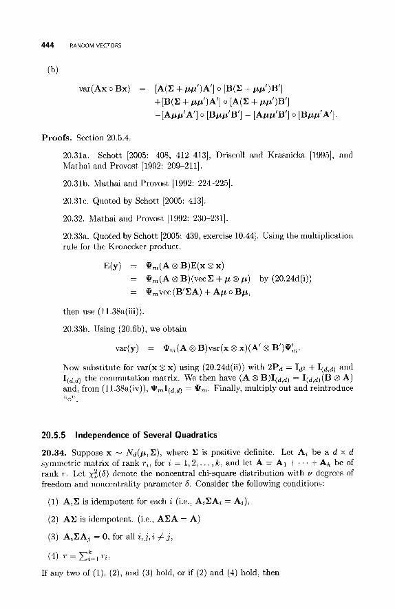
444 RANDOM VECTORS
Proofs. Section 20.5.4.
20.31a. Schott [2005: 408, 412-4131, Driscoll and Krasnicka [1995], and Mathai and Provost [1992: 209-2111.
20.31b. Mathai and Provost [1992: 224-2251,
20.31~. Quoted by Schott [2005: 4131.
20.32. Mathai and Provost [1992: 230-2311,
20.33a. Quoted by Schott [2005: 439, exercise 10.441. Using the multiplication rule for the Kronecker product,
E(y) = *,(A @ B)E(x @ X)
=
=
@,(A @ B)(vec C + p @ p)
9,vec (B’CA) + Ap o Bp,
by (20.24d(i))
then use (11.38a(iii)).
20.33b. Using (20.6b), we obtain
var(y) = Q,(A @ B)var(x @ x)(A’ @ B’)9A.
Now substitute for var(x @ x) using (20.24d(ii)) with 2 P d = Id2 + I(d,d) and I(d,d) the commutation matrix. We then have (A @ B)I(d ,d) = I (d ,q(B @ A) and, from (11,38a(iv)), 9 , I ( d , d ) = 9,. Finally, multiply out and reintroduce “ ,, 0 .
20.5.5 Independence of Several Quadratics
20.34. Suppose x N N d ( p , C ) , where C is positive definite. Let Ai be a d x d symmetric matrix of rank ~ i , for i = 1 , 2 , . . . , k , and let A = A1 + . . . + A k be of rank T . Let xE(6) denote the noncentral chi-square distribution with v degrees of freedom and noncentrality parameter 6. Consider the following conditions:
(1) AiC is idempotent for each i (i.e., AiEAi = Ai),
(2) AC is idempotent. (i.e., ACA = A)
(3) AiCAj = 0, for all i , j ,z # j ,
(4) T = c;=, Ti,
If any two of (l), (2), and (3) hold, or if (2) and (4) hold, then
COMPLEX RANDOM VECTORS 445
(a) x’A,x - x;, (p’Aip) for all i .
(b) X’AX N xF(p’Ap).
(c) x’Alx,. . . , x ’ A ~ x are statistically independent.
The extension of the above result to the case when E is non-negative definite is considered by Mathai and Provost [1992: 2391. When p = 0 and E may be singu- lar, further conditions for quadratics to be independently distributed as chi-square variables are given by Rao and Mitra [1971: section 9.31.
Proofs. Section 20.5.5.
20.34. Schott [2005: 4131.
20.6 COMPLEX RANDOM VECTORS
Complex random vectors arise in several places in statistics, the most notable being multivariate time series (cf. Brillinger [1975: 891) and random matrices (Mehta [2004]).
Definition 20.12. (Complex Random Vectors) Let x = x1 +ix2 and y = y1 +iy2 be complex random vectors, where the xi and yi are all real random vectors. We then define the following:
E(x) = E(x1) + ZE(X~), var(x) = E[(x - Ex)(x - Ex)*], and
~ O V ( X , Y ) = E[(x - Ex)(Y - EY)*],
where x* = xi - ixk.
20.35. Using the notation in the above definition, we readily obtain:
(a) var(x) =V11 +V22+i(-V12+V21), whereVij =cov(x,,xj) , i , j = 1,2 .
(b) COV(X,Y) = cov(xl,Yl) + cov(x2,y2) + i[-cov(x1,y2) + C O V ( X 2 , Y l ) ] .
Definition 20.13. (Complex Normal Distribution) Let x1 and x2 be d x 1 (real) random vectors such that (xi,xk)’ is N2d(,u,E), where p = (pi ,&)’ and
where J? is non-negative definite, and 8 = -8’ (i.e., real skew-symmetric). Then x = x1 Six2 is said to have a complex normal distribution with mean px = p1 +ip2 and variance matrix E[(x-px)(x-pX)*] = Ex, where Ex = El +i& is Hermitian non-negative definite. Here = 2r and E2 = 2@ are real matrices. We say that x - &(pX, Ex). Thus x1 + ix2 is complex normal if and only if
446 RANDOM VECTORS
From (20.35) we can identify
XI = var(x1) + var(xz) and & = -cov(x1, XZ) + cov(x2, XI).
See Mathai [1997: 406-4091 for further details.
20.36. Using the above notation, and assuming that X, is Hermitian positive definite (i.e., !Z1 is positive definite), we have:
(a) (det = det(2X).
(b) EL1 = ( X i + EzET1Ez)-' - iXy1X2(E1 + EzEL'Ez)-'.
(c) The probability density function of x can be written as
1
rd det !Z exp[-(x - p,)*~;'(x -
(d) If x N Ni(p , , Ex) and A is q x d, then Ax - N i ( A p , , A!Z,A*). It follows that the marginal distributions of a multivariate complex normal are complex normal.
(e) If Xz = 0, then XI and xz are statistically independent.
(f) The characteristic function of x is
Eexp[i %e(t*x)] = exp[i %e(t*p,) - t*!Zxt],
where %e is the "real part."
For further background see Krishnaiah [ 19761. Brillinger [1975: 313-3141 gives some asymptotic results for comparing two vector times series.
Proofs. Section 20.6.
20.36. Quoted by Anderson [2003: 64-65].
20.7 REGRESSION MODELS
The study of random vectors would not complete without some discussion of re- gression models. I shall consider mainly linear models, because matrices play a prominent role in these models. Also, other models can sometimes be transformed into linear ones, or else, with large samples, can be approximated by linear ones. There are many good books on linear regression with several different approaches. I personally prefer a geometrical approach using orthogonal projections as developed by Seber [1977, 1980, 19841 and, to a lesser extent, by Seber and Lee [2003]. This approach is being used a lot more in texts because it avoids some of the algebraic manipulations. For the various kinds of linear model see, for example, Christensen [1997, 200ll. An extensive and detailed theoretical treatment of all aspects of linear models is given by Sengupta and Jammalamadaka [2003]. For results on modifying a linear model by, for example, adding or deleting an observation see Section 15.3.
REGRESSION MODELS 447
A typical regression model takes the form y = p + E , where p = (p i ) is an n x 1 vector of unknown parameters, y = ( y i ) , and E = (co) are n x 1 random vectors with E(E) = 0 and var(E) = a2V, where a2 is generally unknown and n x n V may be known. This is usually known as a generalized (weighted) least squares model (cf. Kariya and Kurata [2004], for example). If pi = f(xi;8), where f is a nonlinear function, xi is a known observation, and 0 is unknown, we have a typical nonlinear regression model. The theory of such models is discussed in detail by, for example, Seber and Wild [1989]. In some models, V is known function of p, and quasi-likelihood methods can be used (Seber and Wild [1989: section 2.31). Sometimes V can be a function of other parameters such as autocorrelations in time series models (Seber and Wild [1989: chapter 61) and variances in components of variance models (Sengupta and Jammalamadaka [2003: section 8.31 and Faraway [2006]). We can also have errors-in-variables models where, for example, the xis are measured with error (Seber and Wild [1989: chapter 101 and Carroll et al. [2006]). Other models where p may contain random components are, for example, mixed models and components of variance models (e.g., P.S.R.S R m [1997] and Searle et al. [1992]).
We get another type of nonlinear model when E(y,) = pi, but now g ( p i ) = a + ,@xi and the distribution of yi belongs to the exponential family. This is called a generalized linear model, and such models are discussed by McCullagh and Nelder [1989] and Dobson [2001]. Other transformation methods are described by Carroll and Ruppert [1988], and another approach is via generalized additive models (Tibshirani and Hastie [1990] and Wood [2006]).
Finally, applying large sample maximum likelihood theory to very general prob- ability distributions, we can prove the asymptotic equivalence of large sample tests for nonlinear hypotheses such as the Likelihood ratio, Wuld and Score (Lugrange multiplier) tests by asymptotically linearizing the model and hypothesis. In the linear case, all three test statistics are equivalent (Seber and Wild [1989: section 12.41 and Seber [1980: chapter 111). Examples using this linearization technique are given by Seber [1967, 19801 and Lee et al. [ZOOZ]. We shall now consider the linear regression model.
Definition 20.14. We call the above model y = 0 + E the general linear model if 0 = X p , where X is a known n x p matrix of rank r ( r 5 p < n), and p is a p x 1 vector of unknown parameters. We also assume that V is non-negative definite of rank v, and we shall be interested in testing a linear hypothesis AP = c , where A is q x p of rank s (s 5 q < p ) and c E C(A). We shall refer to the general linear model as M = (y, XP, a2V) and the linear hypothesis as Ho. For making inferences, we shall also assume that y is multivariate normal, namely N , ( X p , a2V).
There have been a large number of theoretical results proved for the above general setup and its special cases. However, my approach to linear models when V is a known nonsingular matrix is somewhat pragmatic: Formulate the theoretical model and hypothesis (e.g., Seber and Lee [2003: section 6.41) and use a statistical computer package such as R to get the required results as well as the diagnostics for validating the model.
If V is a known positive definite matrix, there exists a unique positive defi- nite square root (cf. 10.32) V1/2 so that making the transformation V-1/2y = V-1/2X/3 + V - 1 / 2 ~ we get the model
z = Wp + 77, where var(q) = V-'/2VV-'/2 = I,.
448 RANDOM VECTORS
We therefore begin with the model (y, Xp, a21,). With regard to Ho, we frequently have c = 0. If not we can “remove” c as follows.
Let PO satisfy A& = c and consider the model z = Xy + E , where z = y - Xpo and y = p - 00. Then HO becomes Ay = 0, so for the moment we assume c = 0, which fits in with the method of least squares described below. It should be noted that we can incorporate c if we use a different method of estimation, namely we find af ine unbiased estimators that satisfy a minimum trace criterion (Magnus and Neudecker [1999: chapter 131).
20.7.1
20.37. (Estimation) Consider the model (y, Xp, u21n), where X is n x p of rank r and 8 = Xp.
V Is the Identity Matrix
(a) Assume r < p .
(i) IIy - 8lli is minimized uniquely subject to 8 E C(X) = 0, say, at g, the least squares estimate of 0, where
h
e = pQY, pQ = x(xix)-xi, and PQ is the unique symmetric idempotent matrix representing the orthogonal projection of Y onto 0; (X’X)- is any weak inverse of X’X. Note that y = e^+ (y - g) is an orthogonal decomposition of y , and PQX = X. The matrix Pa is also referred to as the hat matrix in regression diagnostics (Seber and Lee [2003: section 10.21). Other norms and measures can be used for the minimization process to produce alternative estimators to least squares (cf. Gro8 [2003], Rao and Tountenburg [1999], and Seber and Lee [2003: section 3.131.
(ii) If e = Xp , then p is not unique. Since X’(y - 0) = 0 , p satisfies t_he so-called normal equations X‘Xp = X‘y, _which have a solution
h h
h
p = ( x i x ) - x i y = ( x / x ) - x ’ p O y = (xix)-xre. h
(iii) Q = IIy - 011; = y’(1, - Pa)y = €’(In - Pa)€, since (I, - P0)O = 0.
(iv) u2 is usually estimated by its unbiased estimate s2 = Q/(n - r ) , which has certain optimal properties. For example, it is the MINQUE of u2 (Rm and Rm [1998: section 12.61).
(v) r = y - 8 = (I, - P0)y is called the residual vector and is used for diagnostic purposes. Q = r‘r is usually called the residual sum of squares and is often denoted by RSS.
h
(vi) E(r) = 0 and var(r) = a2(I, - PQ).
(vii) For any a, 4 = a‘8 = a’PQy is a linear estimate of 4 = a’@ (i.e., linear
Of all linear unbiased estimates of 4, 3 is the unique estimate with minimum variance. We refer to 3 as the B L U E (Best Linear Unbiased Estimate) of 4.
h A
in y) and is unbiased as PQX = X implies that E($) = 4. (viii) (Gauss-Markov)
REGRESSION MODELS 449
(ix) If B y is any unbiased estimate of 8 , then
D = var(By) - var(8)
is non-negative definite (n.n.d.) and D = 0 if and only if B y = 8. We call 6 the BLUE of 8.
(x) Let y = X P + uu, where the elements of u are i.i.d. with mean zero and variance 1, and density h( . ) satisfying h(-u) = h(u) for all u. Then, provided it exists, the expected information matrix for the parameter vector (P’, a2)’ is
( .Xdx nYmz ) .
h
When u is normal, c = uP2 and I 0 z = l/(2u4).
(b) When X has full rank (i.e., T = p ) then (X’X)- = (X’X)-’ and we have the following:
(i) p = (x’x)-1xr8. (ii) p = (X’X)-’X’y, E(5) = P, and var(P) = u2(X’X)-’.
(iii) From (a) (viii) we find that b’p is the BLUE of b’P. (iv) Suppose the yz are independent random variables with common vari-
ance u2 and common third and fourth moments, p3 and p4, respectively, about their means. Then s2 is the unique non-negative quadratic unbi- ased estimate of u2 with minimum variance when p4 = 3a4 or when the diagonal elements of PQ = X(X’X)-lX’ are all equal.
(v) If, as n + co, n-’X’X converges to a finite positive definite matrix V,, and the largest diagonal element of PQ goes to zero, then fi(p^ - P ) converges in distribution to Nd(0, a2V,).
h
(c) If X has full rank and y - Nn(XP,u21n), then the following hold:
(i) p - N ~ ( P , ~ ~ ( x ’ x ) - ~ ) .
(ii) p is statistically independent of s2 .
(iii) Q/u2 = (n - p ) s 2 / u 2 - &,. (iv) p and Q/n are the maximum likelihood estimates of and u2, respec-
tively, and are also sufficient statistics.
(v) p is the best unbiased estimate of ,d in the sense that, for any b, b‘p is the estimate of b’P with minimum variance among all unbiased estimates, and not just among linear ones; that is, it is the MINVUE of b‘P.
(vi) s2 is the MINVUE of u2.
Definition 20.15. Let X be n x p of rank r. The function b‘P of P is said to be estimable if it has a linear unbiased estimate, c’y, say. Then b‘P = E(c’y) = c‘XP for all P so that b‘ = c’X. Let A’ = (a1,a2,. . . , a4) be a q x p matrix. The hypothesis Ho : AP = 0 is said to be testable if each a# is estimable for i = 1 , 2 , . . . , q, that is AP is estimable. If X has full column rank, then AP is always estimable.
450 RANDOM VECTORS
20.38. Suppose that r < p . The following conditions are equivalent.
(1) A P is estimable.
(2) The rows of A are linearly dependent on the rows of X, that is, there exists a q x n matrix L such that A = LX. If rankA = q, then rankL = q (as rankA 5 rankL, by (3.12)). Note that Ly is a linear unbiased estimator of AP.
(3) C(A’) C C(X’).
(4) A$ is invariant for any choice of p = (X’X)-X’y.
(5) A(X’X)-X’X = A.
20.39. If r < p and A P is estimable, then from (20.38(2)) above we have:
(a) A$ = ~6 = L P ~ ~ = LX(X’X)-X’~ = A(x’x)-x’~.
(b) E(Ap^) = E(L6) = LO = AP.
(c) var(Ap^) = var(L8) = 02LPnL’ = 02A(X’X)-A‘. For a single estimable h
function, A reduces to a’.
20.40. (Estimation with Constraints) Suppose T < p . We wish to find the least squares estimate of P subject to the q estimable constraints A P = 0, that is, subject to o = AP = L X ~ = Lo, or 8 E N(L).
(a) IIy - 011; is uniquely minimized subject to 8 E N ( L ) n R = w, say, when 8 = O H , where 8 H = P,y and P, represents the orthogonal projection onto
A h
W .
h
(b) Q H = I I Y - 8~11; = Y’(L - P,)Y.
(c) From (2.51b) and (2.51d), PQ - P, = PWinn, where w’ n R = C(B) and B = PnL’.
(d) From (c),
6 H = P,y
= P n Y - P w l m Y = 6- B(B’B)-B’y
= 6 - PnL’(LPnL’)-LPny
(e) From (d) and A = LX,
P,i nn = X ( X’X) - A’ [A (X‘X) - A’] -A (X’X) - X’ .
A
( f ) If 6~ = XPH, we have from (d) and (e)
X ~ ^ H = Xp - X(X’X)-A’[A(X’X)-A’]-Ap^.
REGRESSION MODELS 451
If A has full row rank, [A(X’X)-A’]- = [A(X’X)-A’]-l. If, in addition, X has full column rank, then multiplying by X’,
f i ~ = f i - (X’X)-’A’[A(X’X)-lA’]-lAfi. We can also obtain this result using Lagrange multipliers (cf. Seber and Lee [2003: 601.
(g) If we now want to change the constraints to AP = c, where c E C(A), we replace f i by f i - PO (where A,& = c for some PO), Afi by Afi - c, and y by y = y - XPo. QH then becomes y’(In - Pw)y, and Q remains unchanged as (I, - Pn)Y = (I, - Pn)y.
(i) Given the estimable constraints AP = c, another approach is to note that AP = c if and only if ,6 = A-c+(I,-A-A)& where (cf. 13.4) 4 is arbitrary, and A- is any weak inverse of A. Substituting for 0, the constrained model then becomes
(y - XA-c, X(1, - A-A)q5, 021n).
A reasonable choice for A- is A’(AA’)-.
A second approach is use the model (y*, X,P, 02V), where
Y*=(:), X * = ( Z ) , v = ( ‘d. ;), and V is singular (Sengupta and Jammalamadaka [2003: 123, 125, 2441).
20.41. (Hypothesis Testing) Suppose we wish to test HO : AP = c (c # 0), where HO is testable, and A is q x p of rank s (s 5 4 ) .
(a) From (20.40g) and (20.40e),
QH - Q = f ’PwlnnY 1 (A6 - c)’[A(X’X)-A’]-(Afi - c).
(b) E(QH - Q) = 0’5 + (AP - c)’[A(X’X)-A’]-(AP - c).
(c) The test statistic for HO is
(d) When Ho is true, we have the following.
(i) P w l n n y = Pw~nn[y-XP-(XP-XPo)] = P w l n w E , since from (20.40d) with B’ = LPn we have
LPnX(P - P o ) = LX(P - Po) = AP - c = 0.
(ii) If y - N,(XP, u21n), then from (i) the following ratio has an F-distribution, that is.
452 RANDOM VECTORS
Definition 20.16. (Multiple Correlation) Consider the linear model yi = Po + p i ~ i i + P 2 ~ i 2 + . . . + P p - i x i , p - ~ + ~i so that X = (l, ,x(’), . . . , d p - ’ ) ) , where rank X = p . If we define 7 = 8, the correlation coefficient of y and the fitted model 7 is called the multiple correlation coefficient, and is denoted by R. Its square R2, is called the coefficient of (multiple) determination.
20.42. If $ = Cy=l yi/n, then:
h
(a) (y - 7)’1, = 0.
(b) cy=1(Yi - $IZ = cy=“=1(Yi - a2 + E;=l(Gi - !#.
(d) RSS = Ci(yi - Gi)2 = (1 - R2) Ci(yi - j j ) 2 .
Proofs. Section 20.7.1
20.37a(i). Seber and Lee [2003: 36-37].
20.37a(ii). Seber and Lee [2003: 381.
20.37a(iv). Seber and Lee [2003: 441.
20.37a(vi). Use (20.6b). Seber and Lee [2003: section 10.21.
20.37a(viii). Seber and Lee [2003: 42-43].
20.37a(ix). PQ is symmetric and idempotent. Because By is unbiased, (I, - B)8 = 0, so that C[(I, - B)’] I R and PQ = PQB’ = BPa. This leads to D = B(1, - PQ)B’, which is non-negative definite (n.n.d.) as I, - PQ is n.n.d. Finally, D = 0 if and only if (I, - PQ)B’ = 0 or B = PQ.
20.37a(x). Sengupta and Jammalamadaka [2003: 133; they omit the word “expected’] and Seber and Lee [2003: 49, for the normal case].
20.37b(ii). Seber and Lee [2003: 421.
20.37b(iv). Seber and Lee [2003: 451.
20.37b(v). Sen and Singer [1993: section 7.21.
20.37~. Seber and Lee [2003: 47-48 for (i)-(iii); section 3.5 for (iv); 50 for (v)] and Rao [1973a: 319 for (vi)].
20.38. Searle [1971].
20.41b. Use (20.18b) with E(A@ = AP and traceP,lnQ = s.
20.41d(ii). Seber [1977: section 4.51.
20.42. Seber and Lee [2003: 111-1131.
REGRESSION MODELS 453
20.7.2 V Is Positive Definite
20.43. The results for V, a known positive definite matrix, follow directly from the results for V = I, by replacing y by V-1/2y, 8 by V-1/28, and X by V-1/2X through all the previous theory. For example, we now minimize (y - 6)’V-l (y - 8 ) subject to 8 E Q to obtain 8, say. We can do this by changing the inner product space or, more simply, by using the transformation V-1/2 so that X’X becomes X’V-’X and X‘y becomes X’V-ly, giving us
v-1/28 ~ ~ ~ / ~ ~ ( ~ ’ ~ - ~ ~ ) - ~ ’ ~ - ~ y .
Assuming rankX = p , and setting 8 = Xp, we now have two unbiased estimates of P, namely
p = (X’X)-’X’y and p = (x’v-1x)-1x’v-’y
Then using (20.6b),
A
var(P) = a2(X’X)-’X’VX(X’X)-’ and var(p) = a2(X’VX)-l .
The above estimators are often called the ordinary least squares estimate OLSE(P) =
p and the generalized least squares estimate GLSE(P) = p. As 6 is the BLUE of 0, we can expect this estimator t o be more efficient in some sense than 0. Various measures of efficiency are given in (12.6), and a popular one is the Watson efficiency 4 = l/El, where
h
where m = min{p, n - p } and A1 2 A2 2 . . . 2 A, > 0 are the eigenvalues of V . El = 1 if and only if the two estimators are the same. The ratios 4AiA,-i+l/(Ai + A , - ~ + I ) ~ are the squared antieigenvalues of V (cf. Section 6.7), and the pi can be h
taken as the canonical correlations between the OLSE 8 and its residual r = y - 8. For references on the topic see Drury et al. [2002] and the survey by Chu et al. [2005b].
The Watson efficiency has also been applied to partitioned regression models
A
where X and V have full rank. A subset Watson ef ic iency can be defined for the estimate of Pi , and the overall efficiency factorized into components. For details and examples see Chu et al. [2004; 2005a,b].
454 RANDOM VECTORS
20.7.3 V Is Non-negative Definite
We now assume that V is a known singular matrix of rank w (w < n) and that rankX < rankV. For a thorough review and historical summary of the topic see Puntanen and Styan [1989]. Theoretical details are given by Sengupta and Jammalamadaka [2003: chapter 71, Baksalary et al. [1990], and, more briefly, by Christensen [2002]. Singular models arise, for example, in finite population sampling, in some experimental designs, in some state-space models, and in models where some of the y-variables are virtually error-free and are effectively constants.
20.44. Consider the model (y,Xp,a2V), where V is singular and r ankX = T
T < p ) . Let H = Po and M = I, - Po = I, - H, so that from (20.37a(i)) 8 = Hy. L -
(a) The model is consistent (i.e., the inference base is not self-contradictory) if y E C(X, V) with probability 1. This follows from the fact that y - Xp E C(V) with probability 1.
(b) One expression for the best linear unbiased estimate (BLUE) 8 t of 8 takes the form 8 t = Gy if and only if G(X, VM) = (X, 0) (Puntanen et al. [2000]). The numerical value of 8 t is unique with probablity 1, but G is unique if and only if C(X, V) = R".
When V is nonsingular, 8 t = 8 (cf. 20.43).
(c) One general solution to G ( X , V M ) = (X, 0) is
G = I, - VM(MVM)-M + F[I, - M V M ( M V M ) - M ,
where F is arbitrary.
(d) (i) Some representations of 8 t are
e t = ~ - H V M ( M V M ) - M ~
= 6- HVM(MVM)+M~
= 6- HVM(MVM)+~
= y - V M ( M V M ) - M y .
(ii) Also 8 t = X( x' w - X) - X' w - y ,
where W = V + XUX' and U is an arbitrary matrix such that C(W) =
C(X, V ) .
(e) If X has full column rank and 8 t = X p t , then 0' = (X'X)-'X'Bt
( f ) 8t is invariant to the choice of (MVM)-.
(g) Asymptotic theory for 8 t is given by Sengupta and Jammalamadaka [2003: 5221.
(h) (Mean and Variance)
( i ) Since E(My) = MX8 = 0, it follows from (d) that E(8t) = 8.
REGRESSION MODELS 455
(ii) From (d) and HM = 0,
va r (d ) = a2[HVH - HVM(MVM)-MVH]
= a2[V - VM(MVM)-MV]
= a2[X(X’W-X)-X’ - XUX’].
(iii) If X has full column rank and 81 = XPt, then
A
var(Pt) = var(P) - (x’x)-~x’vM(MvM)-Mvx(x’x)-~,
where va@) = (X’X)-lX’VX(X’X)-’.
(i) The residual is
r = y - e +
= My + HVM(MVM)-My
= VM(MVM)-My,
and var(r) = a 2 ~ ~ ( ~ ~ ~ ) - ~ ~ .
(j) Let f = rank(V, X) - rank X. The weighted residual sum of squares is
Qt = (y - Ot)’V-(y - et) = y’M(MVM)-My,
and E(Qt l f ) = c2
(k) If AP is estimable, then the BLUE of AP is
(Ap)t = AX-[I, - VM(MVM)-M)]y.
Furthermore,
~ a r [ ( A p ) ~ ] = a2AX-[V - VM(MVM)-MV](AX-)’
(1) (Inverse Partitioned Matrix Approach) Let
v x ( X ’ (I)-=( 2 2).
(i) e+ = x c k y = XC3y.
(ii) var(8t) = a2XC4X’.
(iii) r = VCly.
(iv) Referring to (j) , Qt = y’Cly.
(m) Ot = e if and only any one of the following conditions hold.
(1) HV = VH.
(2) VV = HVH.
456 RANDOM VECTORS
(3) HVM = 0.
(4) C(VX) c C(X).
For these and further conditions see Puntanen and Styan [1989, 20061 and Isotalo et al. [2005b: chapter 61.
20.45. If X has full column rank p and C(X) C_ C(V), the so-called weakly singular model, then the Watson efficiency is
[det (X'X)I2 ' det(X'VX) . det(X'V+X)
where m = min{p, u - p } and h is the number of nonzero canonical correlations be- ween the ordinary least squares estimate and its residual (Chu et al. (2004, 2005al). These authors have also applied the Watson efficiency to partitioned regression models for the case when V is positive definite. The result about the canonical correlations still applies. For other bounds on the efficiency for the singular model see Sengupta and Jammalamadaka [2003: 316-3181.
20.46. Let U = {U : 0 3 U 3 V,C(U) C(X)}, where A 5 B means that B - A is non-negative definite. The maximal element U in U is called the shorted matrix (operator) with respect to X, and is denoted by S(V I X). Then
var(Ot) = S(V I x). For further references relating to shorted matrices see Mitra and Puntanen [1991], Mitra and Puri [1979], and Mitra et al. [1995].
20.47. (Linear Restrictions) Suppose that we are interested in the linear (es- timable) restrictions A P = c. Let QL be the residual sum of squares after fitting the model subject to the constraints.
(a) QL - Qt = [(AP)t - c] ' [~-~var (AP) t ] - [ (AP) t - c].
the k-distribution, where f = rank(V,X) - rankX, m = rank[var(AP)t], and Qt is given in (20.44j).
Proofs. Section 20.7.3.
20.44a. Christensen [2002: 101 and Rao [1973a: 2971.
20.4413. GroB [2004], Puntanen et al. [2000], and Rao [1973b: 2821.
20.44~. Rao [1978: 12021.
20.44d. See Rao [197313]. The last expression for Ot is derived by Sengupta and Jammalamadaka [2003: 252, with L = I].
OTHER MULTIVARIATE DISTRIBUTIONS 457
We use the fact that (MA)+M = (MA)+ for any A such that (MA)+ exists, since (MA)+M satisfies the four conditions for it to be the Moore-Penrose inverse of MA, and M is idempotent.
20.44f. Sengupta and Jammalamadaka [2003: 2521.
20.44h(iii). Isotalo et al. [2005b: 111.
20.441. Sengupta and Jammalamadaka [2003: 253-2551,
20.44j. Sengupta and Jammalamadaka [2003: 259-2601,
20.44k. Sengupta and Jammalamadaka [2003: 252, 2551.
20.441. Rao [1973b] and Sengupta and Jammalamadaka [2003: 2691.
20.47. Sengupta and Jammalamakada [2003: 277, 2881.
20.8 OTH E R M U LTl VA R I AT E D I S T R I B U T I0 N S
In this section we consider a number of continuous multivariate distributions. These distributions can be regarded as special cases of matrix variate distributions (cf. Section 21.9).
20.8.1 Multivariate &Distribution
Definition 20.17. A d x 1 random vector x = 5 1 , 5 2 , . . . ,zd)‘ has a multivariate t-distribution if its probability density function is given by
( - co<z~<co , i = 1 , 2 , . . . , d),
where X = (gij) is positive definite and I?(.) is the Gamma function. We write x N td(v,p,X). The distribution td(lrO,Id) is called the multivariate Cauchy distribution.
20.48. Suppose x - td(v, p, X), then:
(a) E(x) = p and var(x) = vX/ (v - 2) (n > 2).
(b) (xz ~ p t ) / & - t,, where t, is the univariate t-distribution with v degrees of freedom.
(c) (x -p ) ’X- ’ (x -p) /d - Fd ,” , where Fd,” is the univariate F-distribution with d and v degrees of freedom, respectively.
(d) Any subset of x has a multivariate t-distribution.
For further details see Kotz and Nadarajah [2004]. They also give a number of probability integrals and discuss the noncentral t-distribution.
458 RANDOM VECTORS
20.8.2 Elliptical and Spherical Distributions
Definition 20.18. A d x 1 random vector x is said to have an ellaptical distribution with parameters p ( d x 1) and V (d x d ) positive definite if its density function is of the form
cd(detV)-l12h[(x - p)’V-’(x - p)]
for some function h. We will write x N Ed(p,V) to denote that the distribution belongs to the class of elliptical distributions. The name comes from the fact that the above probability density function is constant on concentric ellipsoids
(x - p)’V-l(x - p ) = c ,
and an alternative name is elliptically contoured distribution. The multivariate t , multivariate normal, the contaminated normal, and a mixture of normal distribu- tions are examples of elliptical distributions. Fang et al. [1990], Gupta and Varga [1993], and Kollo and von Rosen [2005: section 2.31 discuss these and other ex- amples of elliptical distributions. The kurtosis for elliptical distributions need not be zero, so that its typical bell-shaped surface can be more or less peaked than the multivariate normal. This flexibility allows one to study the robustness of sta- tistical inference based on the normal distribution. For the theory and statistical inference based on samples from elliptical distributions see Anderson [1993; 2003, section 3.61, Fang and Anderson [1990], and Kariya and Sinha [1989]. For some asymptotic theory see Anderson [2003: 102, 1581. Matrix versions of the elliptical distribution are also available (Anderson [2003] and Girko and Gupta [1996]).
20.49. Let X N Ed(p, v).
(a) For some function $, the characteristic function of x is
@(t) = E(ezt‘x) = eitfP $(t’Vt).
(b) From (a) we have that any subset of x has an elliptical distribution of the same form. For example, if x1 and p1 are the first lc elements of x and p respectively, and V11 is the leading principal k x k submatrix of X , then x1 &(plrV11).
(c) Provided they exist, E(x) = p and var(x) = aV for some constant a. In terms of the characteristic function a = -2$’(0).
(d) It follows from (c) that all distributions in the class &(p, V) have the same mean p and the same correlation matrix corr(x) = ( p z 3 ) . Since a cancels out, we have pz3 = uz3/(u2zu33)1/2.
(e) Let X = -2$’(O)V = ( ~ 7 % ~ ) be the variance matrix of x, and suppose that x has finite fourth moments. Then:
(i) The marginal distributions of the 2, all have zero skewness and the same
where r;, is the r th cumulant.
OTHER MULTIVARIATE DISTRIBUTIONS 459
(ii) All fourth-order cumulants are determined by K , namely
K v k l - 1111 - K ( ~ y ~ k l + czkcj31 + c d c j k ) .
This result is useful in asymptotic theory relating to smooth functions of elements of the sample variance matrix.
20.50. Let x - J!&(p,v), where v is diagonal. If ~ 1 , z2,. . . ,z, are mutually independent, then x is multivariate normal.
20.51. Suppose x N &(p, V) and x, p, and V are partitioned as follows:
where x1 and ,ul are k x 1 and V11 is k x k . Provided the following exist, then:
(a) E(x1 I x2) = PI + V12V,-,’(x2 - ~ 2 ) .
(b) var(x1 I x2) = g(x2)(V11 - V12V;;V21) for some function g. Moreover, the conditional distribution of x1 given x2 is k-variate elliptical. If g(x2) is a constant so that var(xlIx2) does not depend on x2, then x must be normal.
Definition 20.19. A d x 1 random vector x is said to have a spherical distribution if x and Tx have the same distribution for all d x d orthogonal matrices T. If x has a density function, then this function depends on x only through x’x. The multivariate normal Nd(0, a21d) and the multivariate t, td(v, 0, c 2 1 d ) , are spherical distributions.
20.52. If x - &(o, I d ) , then x has a spherical distribution with a density function of the form cdh(x’x). Let
x1
x2
23
= r sin 81 sin 82 . . . sin 8d-2 sin 8d-1
= T sin 81 sin 8 2 . . . sin 8d-2 cos Od-1
= r sin 81 sin 82 . . . cos 8d-2
zd-1 = rsin81 cos&
xd = rcos81,
where r > 0, 0 < 8i 5 7r ( i = 1,2 , . . . ,d - 2), and 0 < 6d-1 5 27r. Then r, el , 02, . . . , 8 d p l are independent, and the distributions of 81,. . . , 8 d - l are the same for all x, with Ok having a probability density function proportional to 6 k
(so that 8d-1 is uniformly distributed on (0,27r)). Also y = x’x = r2 has probability density function
In particular, if x N Nd(O,Id), we have h(y) = eCYl2 leading to the familiar result that y - x;.
460 RANDOM VECTORS
20.53. Let x have a d-dimensional spherical distribution with pr(x = 0) = 0.
(a) If u = llxll2 = (x’x)’/~ and y = IIxIIzlx, then y is uniformly distributed over a d-dimensional sphere located at the origin with unit radius, and y and u are independent.
(b) If w = a’x/IIx112, where a E Rd and a’a = 1, then
the t-distribution.
(c) If A is a d x d symmetric idempotent matrix of rank k, then z = X’AX/X’X has a beta distribution with parameters i k and $(d - k ) .
Proofs. Section 20.8.2.
20.49. Muirhead [1982: 34-42].
20.50. Muirhead [1982: 351.
20.51. Muirhead [1982: 361.
20.52. Anderson [2003: 47-48] and Muirhead [1982: 36-37].
20.53. Muirhead [1982: 38-39].
20.8.3 Dirichlet Distributions
Definition 20.20. Let x = (51, 5 2 , . . . , zd)’ be a d x 1 random vector. Then x is said to have a Type-l Dirichlet distribution if its density function is given by
(0 < xi < 1, i = 1, . . . , d, z1 + . . . + xd < 1, and ai > 0 for i = 1,. . . , d + 1.)
We shall write x N Dl(d, a) , where a = (ai) .
given by Also x is said to have a Type-2 Dirichlet distribution if its density function is
(0 < 2, < 00, i = 1,. . . ,d , and ai > 0 for i = 1 , 2 , . . . , d + 1.
We shall write x N D2(d, a). The above are special cases of the matrix versions in Section 21.9.
20.54. Let y1, y2,. . . , ym be independently distributed as x 2 variables with degrees of freedom al, a2,. . .am, respectively. If x, = yi/ Cj”==, y j for i = 1 , 2 , . . . , m - 1, then x - D l ( m - 1, a/2) .
Proofs. Section 20.8.3.
20.54. Anderson [2003: 290, quoted in exercise 7.361.
CHAPTER 21
RANDOM MATRICES
21.1 INTRODUCTION
Matrices of random variables occur frequently in statistics, especially in the sub- ject of multivariate analysis. Because the latter is a large subject with numerous reference books, I have had to be somewhat selective in my choice of topics. In this chapter, as in the previous one, the upper- and lowercase letters of the alphabet from a to t , excluding Q, refer to constants, while the remainder generally refer to random variables. Unless otherwise stated, all vectors and matrices are real.
Definition 21.1. Let
be an n x d matrix of random variables with rows that all have the same variance matrix X and are uncorrelated,that is,
cov(x,, xs) = b , J ,
where b,, = 1 for r = s and 6,, = 0 for r # s. We shall call a matrix with the above properties a data matrix.
A Matrix Handbook for Statisticians. By George A. F. Seber Copyright @ 2008 John Wiley & Sons, Inc.
461
462 RANDOM MATRICES
In practice, the x, are usually a random sample, which implies they are indepen- dently and identically distributed, that is, i.i.d. However, this won’t be assumed unless indicated.
21.1. If xi defined above has mean pi for each i, then E(xixg) = 6,jC + pip;.
21.2. (Some Vec Properties) Let X be a data matrix as defined above; that is, the columns of X’ are uncorrelated and have the same variance matrix C. Here “@’’ is the Kronecker product.
(a) var(vecX) = C @I, and var(vecX’) = I, @ C.
(b) Using vec(AXB) = (B’ @ A)vecX, we have, from (20.6b), ( l l . l e ) , and ( 11.1 la) ,
var[vec (AXB)] = (B’ @ A)(C 8 I,)(B’ @ A)’ = (B’XB) 8 (AA’).
(c) var[vec (AX’B)] = var[(B’ @ A)vecX’] = (B’B) @ (ACA’).
(d) cov[vec (AXB),vec (CXD)] = (B’XD) @ (AC’).
(e) From (d) we see that if U = AXB and V = CXD, then U and V are pairwise uncorrelated, that is c o v ( u i j , ~ , ~ ) = 0 for all i , j , T , and s, if AC’ = 0 and/or B’CD = 0.
Proofs. Section 21.1.
21.1. Set xi = xi - pi +pi and use (20.5).
21.2. For (a), see Henderson and Searle [1979: 78, with our X being their X’]; using (20.6), the proofs of (c) and (d) are similar to (b); and (e) follows from (d).
21.2 GENERALIZED QUADRATIC FORMS
21.2.1 General Results
Definition 21.2. If X = (XI, x2,. . . , x,)’ is an n x d data matrix and A = ( u Z J ) is a symmetric n x n matrix, we shall call the expression X‘AX = CZ, C,”=, u ~ ~ x , x ( ~ a generulzzed quadratzc.
21.3. Using the above notation, let T? = Cr=l x,/n and X = (XI - X, . . . ,x, -%)‘. Then:
-
n n - - (a) x’x = C(x, - x)(x2 - x)’ = EX.~: - nxx’ = X’AX (= Q, say),
2=1 2 = 1
where A = ( u Z 3 ) and az3 = 6,, - n-’. Thus, A = I, - l , lh/n = I, - P1 is the so-called centering matrix, where P1 is the orthogonal projection onto (-71,).
(b) Suppose the x, are i.i.d. with mean p and variance matrix C, and S = Q/(n- 1) Then
E(S) = C,
GENERALIZED QUADRATIC FORMS 463
so that S, the so-called sample variance matrix, is an unbiased estimator of E. Some writers define k = (n - l)S/n to be the sample variance matrix; it is the maximum likelihood estimator of C under normality assumptions.
(c) If diag(s) is the diagonal matrix whose elements are the diagonal elements of S, then the sample correlation matrix is given by
R = [ d i a g ( ~ ) ] - ~ / ~ S [ d i a g ( s ) ] - ~ / ~
(d) The (sample) Mahalanobis distance
0,” = (x2 - X)’S-l(xi - X)
- - - is the i th diagonal element of (n - l)X(X’X)-’X, and it is often used for diagnostic purposes.
(e) (i) Taking the trace of (a) and using trace(cd’) = trace(d’c) = d’c, we get
n n
C(X2 - %)’(Xi - x) = c x:xz - nx’x. i=l i=l
(ii)
r=l s=r+l
n
= 7 1 C ( X i - x)(xz - x)’ i= 1
(iii) Taking traces in (ii),
n n n
r=l s=r+l 2 = 1
This result arises in cluster analysis.
We obtain the corresponding univariate cases by taking d = 1 in the above results.
21.4. (Asymptotic Sample Theory) Suppose that the d x 1 vectors X I , x 2 , . . . , x, are independently and identically distributed (i.i.d.) with mean p and variance matrix X .
(a) As n + m, f i ( X - p ) is asymptotically distributed as Nd(0, E).
(b) Let Q = (n - 1)s.
(i) As n + 00, n-1/2(vecQ - nvecE) is asymptotically N d z ( 0 , V), where
V = var{vec [(x2 - p)(x2 - p ) ’ ] } = var[(x2 - p ) 8 (xz - PI] ,
by (11.15~).
(ii) In terms of S, we have (n-l)’/’(vec S-vec E) is asymptotically N,j2(0, V).
464 RANDOM MATRICES
(c) If A is a real symmetric n x n matrix, then, under certain conditions, Q = X‘AX is asymptotically normal as n + 00.
For further details and references see Mathai and Provost [1992: section 4.6bI.
21.5. (Asymptotic Theory) Suppose $(y - 8 ) is asymptotically N d ( 0 , E), and let f(u) be a q-dimensional vector-valued function of u such that each component f,(u) has a nonzero differential at u = 8. If F = (f,,), where f,, = af,(u)/du,, then
&[f(u) - f(8)] is asymptotically N,(O, F’EF).
21.6. Suppose X’ has columns x,, then
n n
E(X’AX) = c c a z , ~ o v ( ~ , , x,) + E(X’)AE(X). 2 = 1 ,=1
21.7. Suppose the x,, the columns of X’, are statistically independent and var(x,) =
X, for z = 1 , 2 , . . . , n. Then, from (21.6),
n
(a) E(X’AX) = C a , , ~ , + E(x’)AE(x). 2 = 1
(b) If E, = E for all a , then from (a) we have
E(X’AX) = (traceA)E + E(X’)AE(X).
(c) Suppose that the x, are i.i.d. with mean 0 and variance matrix E. If V = X’X and E(x,x: 8 x,x:) = !P, then
var(vecV) = n[!P - (vecE)(vecE)’].
21.8. (Independence) Let X’ = (x1, xa, . . . , xn), where the x, are independently distributed as Nd(p , , E) (i = 1 ,2 , . . . , n) and E is positive definite. Suppose A and B are n x n symmetric matrices and C is a k x n matrix. Then:
(a) X’AX and X’BX are statistically independent if and only if AB = 0.
(b) CX and X’AX are statistically independent if and only if CA = 0. Setting C = b’, we have that X’b and X’AX are statistically independent if and only if Ab = 0.
More generally:
(c) Let Q, = X’A,X + f (L,X +X’L:) + C , , where A, and C, are real symmetric matrices (i = 1,2) . Then Q1 and Q2 are statistically independent if and only if
AlA2 = 0, LlA2 = 0, L2Al = 0, and L1Lh = 0.
We can get various special cases by setting A, = 0 or L, = 0. Mathai and Provost [1992: 286-2871 also give results for the case when E is singular.
Proofs. Section 21.2.1
21.3a-b. Seber [1984: 8-91.
GENERALIZED QUADRATIC FORMS 465
21.4a. Anderson [2003: 86-87] and Muirhead [1982: 151.
21.4b. Anderson [2003: 871 and Muirhead [1982: 181.
21.5. Anderson [2003: 1321.
21.6. Mathai and Provost [1992: 2441.
21.7a. Seber [1984: 6-71,
21.7~. Schott [2005: 424-4251.
21.8a-b. Mathai and Provost [1992: 2851 and Schott [2005: 422-4241,
21.8~. Mathai and Provost [1992: 286-2871.
21.2.2 Wishart Distribution
Definition 21.3. Let X = (XI, x2,. . . , xn)’ be an m x d matrix with rows which are independently and identically distributed (i.i.d.) as the multivariate normal distribution Nd(o ,E) , subject t o two conditions, namely (i) d 5 m and (ii) E is positive definite. If W = X’X, then W is said to a have a (nonsingular) Wishart disribution with m degrees of freedom and we write W - Wd(m,E). The joint probability probability density function of the distinct elements of the symmetric matrix W (the i d ( d + 1) variables in the upper triangle, say) is given in (21.67). This Wishart distribution can, of course, be defined directly in terms of its den- sity function, though the above represention is more convenient for developing the theory, especially in the singular case. If a t least one of the two conditions does not hold, then the distribution is said to be singular (cf. Srivastava [2003] for some details). We use m instead of n here as X is used as a “representation” rather than coming from a particular random sample of size m. If W - Wd(m, E) , then we can simply choose any matrix X with rows which are i.i.d. Nd(0,E). Then X’X has the same distribution as W and can be used as a “proxy” for the latter. For this reason, most authors simply set W = X’X (e.g., Seber [1984: 211). For other general references relating to the Wishart distribution see Anderson [2003] and Muirhead [1982]; in fact most theoretical books on multivariate analysis cover the Wishart distribution in detail.
If the xi are independently distributed as N d ( p i , E) with E positive definite, then W = X‘X has a noncentral Wishart distribution, generally written as Wd(m, C; A), where
A = E - ~ / ~ M / M E - ~ / ~ , M = (pl,pz,. . . ,pm)/ = E(x),
and Ell2 is the positive square root of E (cf. 10.32). Here A is called the noncen- trality matrix and, since the distribution of W depends only on the eigenvalues of A, other expressions are used for the noncentrality parameter (Seber [1984: sec- tion 2.3.31). Muirhead [1984: section 10.31 defines A = E-lM’M and gives the probability density function of the noncentral distribution and its properties.
When W has a nonsingular distribution, W-l is said to have an inverted Wishart. For some details see Anderson [2003: section 7.71 and Muirhead [1982: 113, exercise 3.61. A generalized version also exists (Brown [2002]).
466 RANDOM MATRICES
21.9. An important special case is when the x, are all N d ( 0 , u 2 1 d ) . Then the elements of X are all i.i.d. N ( 0 , u2) and X’X - Wd(m, I d ) .
21.10. If the x, ( i = 1 , 2 , . . . , m) are independently distributed as Nd(p, , E) with E positive definite, then using (21.2a) we have
vec (X’) N Nmd (vec (M’) , I, 8 E) ,
where M = ( p l , p 2 , . . . ,,urn)’.
21.11. Suppose W = X’X - Wd(m, E; A), where X is defined above. Then:
(a) E ( W ) = mE + M’M, where M is defined above. For this reason, some authors define the noncentrality parameter to be 9 = M’M or even i9 (e.g., Schott [2005: 422]), which have some advantages, as demonstrated in (21.12) below.
(b) var(vecW) = 2P,[d(E 8 E) + E @ M’M + M’M @ E], where P, is the symmetrizer matrix defined in Section 11.5.1.
21.12. If we redefine the parameters of a noncentral Wishart and write W - Wd(m, E; a), where E is positive definite and = M’M, and C is q x d of rank q, then CWC’ - Wd(m, CEC’; CaC’). In terms of the previous notation, we have A = (CEC’) - 1/2 C9C’ (CEC’) - 1 /2 .
21.13. Suppose W = (w,,) has a nonsingular Wishart distribution Wd(m, E).
(a) W is positive definite with probability 1.
(b) The eigenvalues of W are distinct with probability 1.
(c) E ( W ) = mE, which still holds if W is singular.
(d) Let C be a q x d matrix of rank q.
(i) CWC’ - W,(m,CEC’) and is nonsingular.
(ii) Setting C = a’ (a # 0 ) , we have a’Wa - afx:, where
(iii) By choosing C = (I,,O) ( r 5 d ) , or an appropriate permutation of its columns, we see that an r x r principal submatrix of W has the Wishart distribution W,(m, X,,), where E,, is the corresponding r x r principal submatrix of E.
(iv) If W is singular and rankC 5 q, then CWC’ has a singular Wishart
We have the following special cases.
= a’Xa.
distribution.
(e) w,~ /u , , - x:, ( j = 1 , 2 , . . . , d). However, they are not statistically indepen- dent. Also W , ~ / O ~ , is not chi-square for i # j .
( f ) det W/ det X is distributed as a product of d independent chi-square variables with respective degrees of freedom m, m - 1, . . . , m - d + 1.
GENERALIZED QUADRATIC FORMS 467
(9) The moment generating function (m.g.f.) of W = (wij) is
=
= [det(Id - 2UE)]-m/2,
E{ exp [ t race( U W) ] }
where u = u', u,, = t,, and u , k = u k 3 = at,, ( j < k ) . Since this moment generating function exists in a neighborhood of T = 0, it uniquely determines the (nonsingular) probability density function of W and can therefore be used for deriving a number of results given below. The characteristic function is derived by Muirhead [1982: 871.
We have essentially found the m.g.f. of X'X when the columns of X' are i.i.d. Nd(0, C), where E is positive definite. The m.g.f. of X'AX+i(LX+X'L')+C when the columns of X' are i.i.d. N d ( p , E) is given by Mathai and Provost [1992: section 6.41. They also give results for the cases when the x, are correlated and E is singular.
21.14. Let W - Wd(m, E) , where E is possibly singular, and let A be a d x d (not necessarily symmetric) matrix. Then:
(a) E(WAW) = m[EAE + trace(AE)A] + m2EAE.
(b) If m > d + 1, and E is nonsingular, then
1
m - d - 1 1
m - d - 1
(i) E(WAW-~) =
(ii) E(W-'AW) =
[mEAE-' - A' - (traceA)Id].
[mE-'AE - A' - (traceA)Id].
(c) If m > d + 3, and E is nonsingular, then
E( w - AW - l )
- (m - d - 2)E-lAE-l + E-'A'E-' - trace(AE-')E:-' -
(m - d)(m - d - l ) (m - d - 3)
21.15. Suppose that the columns xi (i = 1,. . . , m) of X' are independently dis- tributed as Nd(pi, E) with E positive definite, and A is a symmetric d x d matrix of rank T . Then, if A is idempotent, we have
X'AX N Wd(m, E; A),
the noncentral Wishart distribution with
A = E-'/2M'AME-1/2 and M = (p1, p 2 , . . . ,p,).
The case when the xi are not independent and C is non-negative definite is consid- ered by Vaish and Chaganty [2004: 3821.
21.16. Suppose that m columns of x' are i.i.d. as Nd(o,E), where E is positive definite, and let A and B be m x m symmetric matrices.
468 RANDOM MATRICES
(a) Let X'AX and X'BX have Wishart distributions. They are statistically independent if and only if AB = 0. (This result is generalized in (21.17).)
(b) Let X'AX have a Wishart distribution. Then X'b is statistically independent of X'AX if and only if A b = 0.
21.17. Suppose that the columns x, (i = 1, . . . , m) of X' are independently dis- tributed as Nd(p,, E), and let Al , A2,. . . , A t be a sequence of n x n symmetric ma- trices with ranks rl, r ~ . . . . ,rt such that cf=, A, = I,. If one (and therefore all) of the conditions of (8.78) hold, then the X'A,X ( i = I , 2 , . . . , t ) are independently dis- tributed as the noncentral Wishart, Wd(r,, E; A t ) , where A, = E-1/2M'AzME-1/2 is the noncentrality parameter and M = (p1, p a , . . . , pm)'. An extension of this result to the case when the x, are not independent and E is non-negative definite is given by Vaish and Chaganty [2004: 3831 and Tian and Styan [2005: 3911.
21.18. If W, - Wd(mt,E) ( i = 1,2) , and W1 and W2 are statistically indepen- dent, then W1 + W2 - Wd(m1 + m2, E).
where E is positive definite, W,i is di x d,, ( i = 1,2), and dl + d2 = d. Suppose E is partioned in the same way as W and E22.1 = E22 - E21ET;E12.
(a) We have W22.1 = W22 - W21WF:W12 - Wdz(m - dl, E22.1)~ and W22.1 isstatistically independent of (W11, W12). Note that W12 = Wil.
(b) If El2 = 0, then Y = W21WF;W12 - Wdz(d1,&) and Y is statistically independent of W22.1.
Definition 21.4. (Hotelling's Distribution) Suppose y - Nd(0, E), W - Wd(m, E), y is statistically independent of W, and both distributions are nonsingular. Then
T 2 = my'W-ly
is said to have a Hotelling's distribution, and we write T2 - T&.
21.20. Referring to the above definition, F = - . F-distribution with d and m - d + 1 degrees of freedom, respectively.
with noncentrality parameter S = O'EO.
2 1.2 1. (Eigenvalues)
T;,, m - d + l Fd,m-d+l, the d m
If, instead, y - Nd(8, E), then F - F,+-d+l,h, the noncentral F-distribution
(a) If the probability density function of the m x d matrix Y is f (Y'Y), then the probability density of B = Y'Y is
where r d ( ' ) is given by (21.67)
GENERALIZED QUADRATIC FORMS 469
(b) If the real symmetric d x d matrix C has a probability density function of the are the eigenvahes of c, form g(X1, &, . . . , A d ) , where
then the probability density function of the eigenvalues is > > . . . >
(c) Suppose W N Wd(m,Id). Using (a) and (b), the probability density function of the eigenvalues of W is
( m - d - 1 ) / 2 d d T d 2 / 2 n,“=, A,
2dm/2rd(;m)rd( i d ) 2=1 2<J
exP(-$ CXJ I-p, - X J ) .
(d) Suppose W N Wd(m,X), where m d and C is positive definite. Then the probability density function of the eigenvalues of W is
where A = diag(X1,. . . , A d ) and When E = I,, we have
is a two-matrix hypergeometric function.
0 0 F d ( - i A , I d ) = oFo(-$A, ) = exp(-; trace A),
which gives us (c)
21.22. (Generalized Eigenvalues) Let Wi (i = 1,2) be independently distributed as nonsingular Wd(mi, X) (i.e., m 1 , m2 2 d and C positive definite). The probability density function of the generalized eigenvalues, namely the roots of
det(W1 - XW2) = 0,
is
for 2 ’ ’ ’ 2 Ad 2 0.
Definition 21.5. (Complex Wishart Distribution) Suppose x1,x2,. . . , x , are independently and identically distributed as the complex multivariate normal dis- tribution N ~ ( O , C , ) (cf. Section 20.6), then W = zz ,x ix ,* is said to have a complex Wishart distribution denoted by W$(m, Ex). It is used in approximating the distributions of estimates of spectral density matrices in multivariate time series and in random normal (Gaussian) processes generally. Some of the properties of the (real) Wishart distribution carry over into the complex case. For a number of references see Brillinger [1975: 901.
21.23. Suppose W = (wij) N W2(m,Cx) , where m 2 d and Ex is Hermitian positive definite. Then:
470 RANDOM MATRICES
(a) The probability density function of the distinct elements of W is
(det W)m-d exp [ - trace( X i 1 W)]
7rd(d-1)/2(det Ex), nf=, r(m - j + 1) ’
(b) E(W) = mXx.
Proofs. Section 21.2.2.
21.11a. Follows from (21.7b) with A = I,.
21.11b. Schott [2005: 4251
21.12. Schott [2005: 4231.
21.13. Seber [1984: 21, 27, 561.
21.14. Styan [1989].
21.15. Schott [2005: 4221.
21.16. Schott [2005: 4221 and Seber [1984: 24-25].
21.18. This can be readily proved using moment generating functions (cf. 21.13g).
21.19a. Seber [1984: 50-511 and Schott [2005: 423-4241,
21.19b. Seber [1984: 51-52].
21.20. Seber [1984: 30-311.
21.21a. Anderson [2003: 539, with Y -+ Y’ and p + d].
21.21b. Anderson [2003: 538-5391 proves this using (a).
21.21~. Anderson [2003: 5391 and Muirhead [1982: 389, with X = 1,nli = Xi].
21.21d. For details see Muirhead [1982: 388-389, with X i = nli].
21.22. Anderson [2003: section 13.2, and section 13.6 for some asymptotic theory].
21.23. Srivastava [1965].
21.3 RANDOM SAMPLES
21.3.1 One Sample
21.24. Let x,, i = 1,2, . . . , n, be a random sample from a d-dimensional distribu- tion with mean p and variance matrix X. Let X = (~1~x2,. . . ,x,)’ be the data matrix and let z, = x, - p (i = 1 ,2 , . . . , n). Suppose that the following third and fourth moment matrices exist, namely
= E(z, @ z,z:) and !P = E(z,z: 8 z,z:),
RANDOM SAMPLES 471
where “€3” is the Kronecker product. Let z = (z i , zl,, . . . zi)’ = vec (X’) - 1, @ p so that E(z) = 0 and E(zz’) = var(vecX’) = I,@E (by (21.2a). Define 6, = E(z@zz’) and ** = E(zz’ @ zz’). Then:
(a) If Kd, (I( , ,d) ) is the commutation (vec-permutation) matrix, E,, = e,e: is an n x n matrix with 1 in the ( i , i) th position and zeros elsewhere, and G =
(Ell, E 2 2 , . . . , En,)’, then
8, = (I, @ Kd, @ Id)(G @ a) -
(b) If K,, = C;=“=,E,, 8 Ei,), then
** = ( 1 , ~ + K,d,,d)(L 8 E 8 I, 8 E) + [vec (I, @ E)][vec (I,
+(I, €3
E)]’
8 I d ) { K n n @ [* - (Id2 + Kdd)(E @ E)
-(vet E)(vec E’]}(I, @ Knd @ Id).
(c) Under normality we have the following results.
(i) 8 = 8* = 0.
(ii) If P d = ;(Id2 + Kdd) (the symmetrizer matrix), then, from (20.24b),
9 = 2 P d ( X @ E) + (vec E)(vec E)’.
(iii) ** = 2P,d(I, @ E 8 I, @ E) + [vec (I, @ E)][vec (I, E)]’. Methods for finding E(x @ x €3 x), E(x @ x 8 x 8 x), and higher moments are given by Meijer [2005].
21.25. Let x,, i = 1 , 2 , . . . ,n, be a random sample from a nonsingular normal distribution N d ( p , E). Then:
(4 x - Nd@, E h )
(b) Q = ( T Z - 1)s N Wd(n - 1, E).
(c) From (b) we can obtain the probability density function of the eigenvalues of Q, and therefore those of S. As this joint distribution is rather intractable, asymptotic theory has been developed for large n for both the eigenvalues and eigenvectors of S, especially as related to providing approximate inferential procedures for principal’ component analysis. The reader is referred to Seber [1984: 197-1991 for a summary of the results, and to Anderson [2003: section 13.51, Muirhead [1982: chapter 91, and Schott [2005: 427-4291 for further details and some derivations.
(d) We consider some properties of S. Here P d is the symmetrizer matrix (cf. 20.2413) and Gd is the duplication matrix.
(i) var(vecS) = (n - 1)-l2Pd(E B E) = (n - 1)p12Pd(E 8 E)Pd.
(ii) We note that the above matrix in ( i ) is singular as S is symmetric, which implies that vec S has repeated elements. We can get round this by using the vector vech S. Then
G:Pd(E @ X)PdGi’. 2
var(vechS) = ~
n - 1
472 RANDOM MATRICES
(iii) As n + 00, (n - 1)’/2(vecS - vecx) is asymptotically distributed as Nd2(OIV), where V = 2Pd(C 8 C).
(iv) From vechS = GdfvecS, (20.6b), and (iii), (n - 1)1/2(vechS - vech C) is asymptotically distributed as Nk(0, GdfVGdf’), where k = d(d+ 1)/2.
(v) If s = diag S and n = diag E, then
2 n - 1
E(s) = u and var(s) = -(C o C),
where “0” is the Hadamard product. Also, as n + 00, (n - 1)’l2(s - u) is asymptotically distributed as Nd(0,2C o C).
(vi) Schott [2005: 431-4321 gives the asymptotic variance matrices for vec R and vech R, where R is the sample correlation matrix.
(e) X and S are statistically independent,
( f ) X and S are jointly sufficient and complete for p and C.
(g) A useful statistic is
(i) T2 = n(r? - p)S-’(sI - p ) - T&-’ (cf. 21.20). This statistic can be
(ii) When the underlying data come from an elliptical distribution, T 2 is
used for testing the null hypothesis Ho : p = po.
asymptotically x:. (h) If Ho : p E V , where V is a pdimensional vector subspace of Rd, then we
have the following.
(i) T$in = min,,vT2 - Td-p,n-l.
(ii) If we have Ho : p = KO, where K is a known d x p matrix of rank p and p is a vector of p unknown paramters, then V = C(K) and
T:in = n ( X ’ S I X - X’S-’KP*),
where p* = (K’S-lK)-lK’S-lx.
that V = N(A) , the null space of A. Then (iii) Suppose we have HO : Ap = 0, where A is d - p x d of rank d - p , so
T , ~ ~ = n ( ~ ~ ) ’ ( ~ ~ ~ ’ ) - l ~ ~ .
A slight generalization of this is given in (i) below.
(i) Let A be a q x d matrix of rank q. Then:
(i) n(AsI-Ap)’(ASA’)-’(AX-Ap) N
(ii) If A is a matrix of contrasts so that Ald = 0, then
This can be used for testing Ho : A p = C.
RANDOM SAMPLES 473
Proofs. Section 21.3.1.
21.24. Neudecker and Trenkler [2002].
21.25a-b. Seber [1984: 631.
21.25d(i)-(v). Schott [2005: 426-4271,
21.25d(vi). Schott [2005: 431-4321,
21.25e. Seber [1984: 631.
21.25f. Anderson [2003: 841.
21.25g(i). Seber [1984: 631.
21.25g(ii). Anderson [2003: 199-2001.
21.25h. Seber [1984: 77-79].
21.25i(i). Seber [1984: 721.
21.25i(ii). Seber [1984: 1241
21.3.2 Two Samples
21.26. Let V I , VZ, . . . , v,, be a random sample from N&l, E), w1, w2,. . . , w,, be an independent random sample from Nd(p2, E), and 8 = p1 - p2. Also define Q1 = ~ r ~ i ( v z - V)(vz - V)’ and Q2 = C ~ ~ l ( w z - W)(wz - W)’. Then:
(a) V - W - Nd(8, (n,’ + n2’)X). (b) Q = Q i + Q 2 N Wd(ni + 722 - 2, E).
(c) n1n2(n1 +~~~) - ‘ (v -w-8) ’S ;~ (v -w-8) N Td,,l+nz-2, the T2 distribution (cf. 21.20), where
We can use this statistic t o test HO : 8 = c .
S, = Q / ( T L ~ + 722 - 2).
(d) If C is a q x d matrix of rank q ( q 5 d) , then
This can be used to test HO : C8 = 0. When C is an appropriate d - 1 x d contrast matrix then the methodology relating to HO is referred to as profile analysis.
The topic of more than two samples is best handled as a special case of the multi- variate linear model described in the next section.
Proofs. Section 21.3.2.
21.26. Seber [1984: 108, 1171.
474 RANDOM MATRICES
21.4 MULTIVARIATE LINEAR MODEL
21.4.1 Least Squares Estimation
Definition 21.6. Let Y = 0 + U, where 0 = XB, B is a p x d matrix of unknown parameters, X is an n x p known matrix of constants of rank r ( r 5 p ) , U =
(u l , . . . un)‘ = (u(l), . . . , u ( ~ ) ) , and the ui are a random sample from a distribution with mean 0 and variance matrix E. Then Y = XB + U is called a multivariate linear model. When d = 1, this reduces to the univariate linear model of Section 20.7.
We have introduced a change in notation in this section. Up till now, X has represented a matrix of random variables, whereas now we assume it t o be a matrix of constants. This will be the case if we can carry out any analysis conditional on the observed value of X. However, the use of X is traditional for linear models, and in some cases the elements of X take only values 0 or 1, thus representing qualitative variables. In this case, X is sometimes referred to as the design matrix, though, as Kempthorne [1980: 2491 argues, a better term is perhaps model matrix. The matrix Y now takes over the role of a data matrix. In what follows we let R = C(X).
Definition 21.7. If we partition Y, 0, and B in the same way that we partitioned U, then the j t h column of the multivariate linear model is the univariate model y(J) = O ( J ) = Xp(j) + u(j), where u(j) has mean 0 and variance matrix njjIn. If P,y(j) is the (ordinary) least squares estimate of O ( j ) (cf. 20.37a), where Pa =
X(X’X)-X’, we say that 0 = P a y is the least squares estimate of 0. When T = p , then setting 0 = Xlh we have B = (X’X)-’X’6 = (X’X)-lX’Y, called the least squares estimate of B. If r < p , then B is not unique and we can use (as in the unvariate case) g = (X’X)-X’Y, where (X’X)- is any weak inverse of (X’X).
21.27. yi = B’xi + ui, where xi is the i th row of X.
21.28. If X has full rank, then E(g) = B.
21.29. We have the following covariance properties.
A
h A
h
(a) cov(y,,y,) = cov(u,,u,) = C ~ , ~ X , where 6,, = 1 when r = s and 0 otherwise.
(b) cov(y(j), y(’))) = cov(u(j), ~ ( ~ 1 ) =
(c) If X has full rank p , then p ( j ) = (X’X)-lX’y(j) and
for all j, k = 1,. . . , d.
C O V ( ~ ( ~ ) , @ ~ ) ) = 0. Ik (X’X)-’ (all j, Ic = 1,. . . , d ) .
21.30. Let G ( 0 ) = (Y - 0)’(Y - 0).
(a) (i) E = G ( Q ) = Y ’ ( I ~ - P ~ ) Y = ~ ’ ( 1 , - P,)u. (ii) E(E) = (n - r )X .
(iii) E is positive definite with probability 1.
Here E is sometimes referred to as the error matrix or residual matrix.
(b) G ( 0 ) - G ( 6 ) = (6 - 0)’(6 - 0) is positive semidefinite for all 0 = XB, and equal to 0 if and only if 0 = Q . We can say that 6 is the minimum of the
MULTIVARIATE LINEAR MODEL 475
matrix G ( 0 ) . As a consequence we have the following properties of the least squares estimate from (10.48b,d) and (10.47a(iii)).
(i) traceG(O) 2 t raceG(6) .
(ii) det G(O) 2 det G(@).
(iii) IlG(0)ll~ 2 IlG(6)ll~, where l lA l l~ = {trace(A’A))ll2 and 1 1 . I I F is the Frobenius norm.
Any of these three results could be used as a definition of @.
21.31. (Generalized Gauss-Markov Theorem) If q5 = Cf, hi8(j), a linear com-
bination of all the elements of 0, then 4 = El=, hid(j) is the BLUE of q5 (i.e., the linear unbiased estimate with minimum variance).
21.32. (Two-Sample Case) Setting V’ = (v1,v2,. . . , vn1), W’ = ( ~ 1 , ~ 2 , . . . ,wn,), and Y = (V’, W’)’ we see that the two-sample problem (cf. 21.26) is a special case of the multivariate model with
The extension to n samples is straightforward.
Definition 21.8. If X has less than full rank, then each univariate model also has less than full rank. From (20.38(2)), aIp(j) is estimable for each i = 1,2, . . . , q and each model j = 1 , 2 , . . . ,d if ai E C(X’). Let A’ = (al,a2,. . . , ap ) . Combining these linear combinations, we say that AB is estimable if A‘ = X’L’ or A = L X for some g x n matrix L.
21.33. Suppose AB is estimable.
(a) If A is g x p of rank q, then L has rank q by (20.38(2)).
(b) A@ = LX(X’X)-X’Y = L P n Y = (PnL’)’Y is invariant for any choice of weak inverse (XX’)- as Pa is invariant. Here POL’ is unique (but not L, unless X has rank p ) and has full row rank.
h
(c) 4 = a’ABb = a’L6b is the BLUE of q5 = a’ABb = a’LOb.
(d) A(X’X)-A = LPnL‘ = (PnL’)PnL’ is invariant and nonsingular by (b).
(el E(A@ = L P ~ X B = LXB = AB, since P ~ X = X.
Proofs. Section 21.4.1.
21.27-21.29. Seber [1984: 4001.
21.30a. Seber [1984: 398, 4021.
21.30b. Seber [1984: 397-3981.
21.31. Seber [1984: 400-4011.
21.32. Seber [1984: section 8.6.41.
476 RANDOM MATRICES
21.33b. E(A6) = (PnL’)’O. If (PnM‘)’Y is another estimate, then [PnM’- PnL’1’0 = 0 and C[Pn(M’ - L’]) I C(X) as the columns of 0 are in C(X). Thus, P n M ’ - PnL’ = 0 C[Pn(M’ - L’] C C(X).
21.33~. The result follows from (21.31) by relabeling.
21.4.2 Statistical Inference
Let Y = 0 + U. In this section we now assume that the underlying distribution of the columns u, of U’ is a (nonsingular) multivariate normal distribution Nd(0, E). The case when X is singular is considered by, for example, Srivastava and von Rosen [2002]. The multivariate model can be expressed in terms of the univariate model vecY = vec (XB) + vecU, where from (21.2~~) vec (XB) = ( I d @I X)vecB and var(vecU) = I: 8 I, (cf. Searle [1978]). A more general model in which var(vecU) = I: 8 V, with V and E possibly singular, is considered by Sengupta and Jammalamakada [2003: chapter lo].
21.34. The likelihood function for Y, the density function of vecY (or, more conveniently, vec (Y’)) is the joint distribution of the independent yz, and it can be expressed in the form
(27rPndl2(det E)-n12 exp{trace[ - 2 (Y - 0)’E-’ ( Y - @)I}. 21.35. Suppose 0 = XB, where X has rank r , and let E be given by (21.30a). We assume n - r 2 d. Then:
(a) E - Wd(n - r , E).
(b) E is statistically independent of 6 (and of % if X has full rank p ) .
(c) The maximum likelihood estimates of X, 0, and B (if X has full rank), The maximum value of the likelihood function are % = E/n, 6, and 6.
is (27rPndl2(det %)-n/2e-nd/2. (This corrects a typo in Seber [1984: 4071.)
(d) If X has full rank, then (6, %) is sufficient for (B, E).
(e) Referring to the j t h column of 6, if X has full rank (cf. 21.29c),
p) - N , ( P ( J ) , oJJ (x ’x ) - l ) .
21.36. Suppose that 0 = XB, where X has rank T . Let A be a known q x p matrix of rank q, and let AB be estimable. We are interested in testing Ho : AB = C , where C is a constant matrix. Then:
(a) Referring to (21.30), the minimum EH, say, of G(XB) subject to AB = C occurs when B equals
% H = 6 - (X’X)-A’[A(X’X)-A’]-1(A6 - C ) .
Although B and BH are not unique when r < p , 0 = XB and OH = XBH are unique. Also EH is positive definite with probability one.
h h h h h h
MULTIVARIATE LINEAR MODEL 477
(b) H = EH - E = (A6 - C)I[A(X’X)-AI]-’(A6 - C).
H is positive definite with probability one.
(c) E(H) = qE + (AB - C)’[A(X’X)-A’]-’(AB - C) = qE + D, say, and D is positive definite.
(d) H and E are statistically independent.
(e) When Ho is true, H N Wd(q,E). When HO is false, H has a noncentral Wishart distribution Wd(q, X; A), with noncentrality matrix given by A =
( f ) Let E i 2 be the positive definite square root of EH (cf. 10.32). Then, when
Ho is true, V = E i 1 / 2 H E i ’ / 2 has a d-dimensional matrix variate Type-1 beta distribution with degrees of freedom q and n - r (cf. Section 21.9)
21.37. Four different criterion are usually computed for testing Ho, and are ex- pressed as functions of eigenvalues of V given in (21.36(f)) above.
E-1/2DE-1/2,
1. Roy’s maximum root test &,,, the maximum eigenvalue of HE-’, based on the so-called union-intersection principle.
(det E/ det E H ) ~ / ~ . 2. Likelihood ratio test
3. The Lawley-Hotelling trace (n - r ) trace(HE-l).
4. P illai’s trace trace (HE,‘ )
These tests are summarised by Seber [1984: chapter 81, but for further details and distribution theory see Muirhead [1982: chapter lo].
Proofs. Section 21.4.2.
21.34. Seber [1984: 4061
21.35. Seber [1984: section 8.41.
21.36. Seber [1984: section 8.61.
21.4.3 Two Extensions
We give two extensions to the theory, which demonstrate how matrix theory can be applied.
21.38. (Generalized Hypothesis) Suppose we want t o test HO : ABD = 0, where A is q x p of rank q ( q 5 p ) and D is a known d x w matrix of rank w (w 5 d) . To do this, let YD = YD so that the linear model Y = XB + U is transformed to
YD = XBD + UD = XA + Uo,
say, where the columns of Ub are i.i.d. N,(O, DIED). Then HO becomes AA = 0 and we can apply the previous theory of (21.36) to this transformed model.
478 RANDOM MATRICES
(a) H now becomes HD = D’HD = (A%D)’[A(X’X)-’A‘]-’A%D and E be- comes ED = D’ED - Wv(n - r, D’ED).
(b) When ABD = 0 is true, HD - W,(q,D’XD). The only change to the previous theory is to replace Y by YD and d by v.
(c) The above theory reduces to that of Section 21.4.2 if we set D = Id and v = d.
This hypothesis is used for carrying out a profile analysis of more than two popu- lations (Seber [1984: section 8.71).
21.39. (Generalized Model and Hypothesis) Consider the model
Y = XAK’ + U,
where X is a known n x p of rank p , A is p x k matrix of unknown parameters, K’ is a known k x d of rank k ( k < d) , and the rows of U are independently and identically distributed (i.i.d.) as Nd(0, E). We wish to test the hypothesis
Ho : AAD = 0:
where A is q x d of rank q and D is k x v of rank v. This model is usually called the growth curve model and it is considered, along with extensions, by Pan and Fang [2002] and Kollo and van Rosen [2005: chapter 41. A brief discussion is given by Seber [1984: section 9.71.
One simple approach to the above model when there are appropriate rank con- ditions is to transform the model to remove K’ using a right inverse of K’. One method, suggested by (Potthoff and Roy [1964] and described in detail by Seber [1984: 4791, is to choose a nonsingular d x d matrix G (usually positive definite) such that the k x k matrix K’G-lK is nonsingular, and transform yi to Clyi, where C1 = G-‘K(K’G-’K)-’ is d x k of rank k . Then K’C1 = I k so that
Y1= YC1= XAK’C1+ UC1 = XA + U1,
where the columns of Ui, namely Clui, are i.i.d. N k ( O , X 1 ) with XI = CiXC1. We have now reduced the model to the previous case, and the theory used there for testing Ho can be applied here with Y replaced by Y1 and d by k .
21.5 DIMENSION REDUCTION TECHNIQUES
21.5.1 Principal Component Analysis (PCA)
Given a data set of interrelated variables represented by an n x d data matrix X = (xl, x2,. . . , xn)’, the aim of principal component analysis (PCA) is to reduce the dimensionality d of the data set, while still retaining as much of the variation present in the data set as possible. This is achieved by transforming to a new set of variables, called the principal components, which are uncorrelated and are ordered so that the first few retain most of the variation present in all of the original variables. Also, we would hope that the components may have some physical interpretation.
We shall first look at the underlying population model that generates the data, and then consider the sample estimates of various quantites. There are numerous
DIMENSION REDUCTION TECHNIQUES 479
books on multivariate analysis that contain chapters or sections on principal compo- nents, e.g., Anderson [2003], Krzanowski [1988], Muirhead [1982], and Seber [1984] (which happen to be in my office when writing this). However, more specialized books are available such as Flury [1988] and Jolliffe [2002].
Definition 21.9. Let x be a random d-dimensional vector with mean p and vari- ance matrix X. Let T = (tl, t 2 , . . . , t d ) be an orthogonal matrix such that, by the spectral theorem (cf. 16.44), we have
X t j = X j t j and
where A1 2 X2 2 . . . 2 are the ordered eigenvalues of C. The sum traceC is sometimes called the total variance. If y = (yj) = T’(x - p) , then y j = t$(x - p) ( j = 1,2, . . . , d) is called the j t h population principal component of x. In developing the population theory there is no loss of generality in assuming p = 0.
A major drawback to the above approach is that it can be sensitive to the units of measurement used for each zi. For this and other remons some authors work with the population correlation matrix corr(x) rather than the variance matrix C. For a discussion of the relative merits of the two approaches see Jolliffe [2002: section 2.31. The optimal properties described below for C also apply to corr(x) if we use the standardized vector z = ( z i ) , where zi = (xi - pi)/&, instead of x.
21.40. (Population Properties)
T’CT = A = diag(XI,X2,. . .,Ad),
(a) c = TAT’ = xf=l xitit;.
(b) The principal components define the principal axes of the family of ellipsoids (x - p)’C-l(x - p) = const.
(c) Since t j has unit length, y j is the length of the orthogonal projection of x - p
(d) As var(y) = A, the y j are uncorrelated and var(yj) = X j .
(e) El=, var(yj) = CjE1 var(zj) = t racez, the total variance. We can use A j / trace C to measure the relative manitude of Xj . If the X i (i = k+ 1,. . . , d) are relatively small so that the corresponding yi are “small” (with zero means and small variances), then y(k) = (yl, y2,. . . , yk)’ can be regarded as a k dimensional approximation for y. Thus y ( k ) can be used as a L L p r ~ ~ y ” for x in terms of explaining a major part of the total variance.
It should be noted that the last few components are likely to be more useful than the first few in detecting outliers that are not apparent from the original variables (Jolliffe [2002: 2371).
in direction tj.
d
( f ) Let T ( k ) = ( t i , . . . , t k ) . Then:
(i) max var(a’x) = var(tix) = var[ti(x - p)] = var(y1) = X I , a‘a= 1 so that y1 is the normalized linear combination of the elements of x - p with maximum variance XI.
var(a’x) = var(tkx) = var(yk) = &, so that tL(x - p)
is the normalized linear combination of the elements x - p uncorrelated with y1, y2, . . . , yk-1 with maximum variance Xk.
(ii) max a‘a=l,T{k-,)a=O
480 RANDOM MATRICES
The above results can be expressed in several different ways (e.g., Jolliffe [2002: 11-12]).
(g) (Predictive Approach) Let B be a d x k matrix, and consider the “best” linear predictor of x - p on the basis of B(x - p). The Frobenius norm of the variance matrix of the prediction error is
11x - C B ( B ’ C B ) - ~ B % ~ ~ ~ = llx1’2(~d - P 81/2B)x1/2 II F ,
where P C 1 / z B is a symmetric idempotent matrix representing the orthogonal projection onto C(C’12B). The norm is a minimum when B is equivalent to T(k). Moreover, minimizing the trace of the variance matrix of the prediction error-that is, maximizing trace(P81/2BC)-yields the same result (Jolliffe [2002: 171).
The results ( f ) and (9) above are optimal properties shared by principal compo- nents, and (e) was used by Hotelling [1933] to define principal components. For further properties see Jolliffe [2002: section 2.11 and Seber [1984: section 5.21. A key theorem for developing such properties is given next.
21.41. Let f be a function defined on P , the set of all d x d non-negative definite matrices. For any C E P , let X,(C) 2 X,(C) 2 . . . 2 &(C) 2 0 be the eigenvalues of C. Then f is strictly increasing and invariant under orthogonal transformations if and only if f (C) = g[Xl(C), . . . , Xd(C)] for some g that is strictly increasing in each argument. This means that minimizing f (C) with respect to C is equivalent to simultaneously minimizing the eigenvalues of C. The functions traceC, IJCIIp = [ t r a ~ e ( C C ’ ) ] l / ~ , and det C satisfy the conditions on f .
21.42. Suppose f satisfies the conditions in (21.41) above and v ( k ) is a k-dimensional vector. Then
f (var[x - c1 - AV(k)l)
is minimized when Av(k) = T(k)y(k) = T(k)Tik)(x - p ) = P ( x - p ) , where P represents the orthogonal projection of x - p onto C ( T ( k ) ) .
Definition 21.10. (Sample Components) In practice, p and C are unknown and have to be estimated from a sample X I , x2,. . . , x,, that is the xi are assumed to be @dependently and iceentically distributed. We-can estimate p by f i = X and C by C = X‘X/n, where X is the centered matrix X = (XI - X, . . . , x, - x)’. Carrying out a similar factorization on E as we did for-C, we obtain the eigenvalues A1 2 i2 2 . . . 2 i d > 0 and an orthogonal matrix T = (i1, i 2 , . . . , i d ) of corresponding eigenvectors. For each observation xi we can define a vector of sample (estimated) principal components ?i = T’(xi - X), which gives us
- - -
h
h A -
Y’ = (?1 ,?2 , . . . , Fn) = T’X’.
Many authors prefer to use the unbiased estimator S of I: instead of 5 in defining the sample components. In this case
and the eigenvalues of S are n i j / (n - 1)
DIMENSION REDUCTION TECHNIQUES 481
The question arises as to whether we should use S or the sample correlation matrix R. However, it is much easier t o base any inference about the population components on S rather than on R using large sample theory. A key result is that if x - Nd(p,x) , then from (21.25b), (n - 1)s - Wd(n - 1,E) . For aspects of large sample theory see Seber [1984: section 5.2.51 for a brief summary. For further details see Anderson [2003: section 11.61 and Muirhead [1982: chapter 91, and see Kollo and Neudecker [1993, 19971 with regard to elliptical distributions. We note that the theory can be modified to handle dependent data such as a time series (Jolliffe [2002: chapter 121). Also, PCA can be used in conjunction with other multivariate techniques (Jolliffe [2002: chapter 91. With some adaption, it can be used for discrete data like contingency tables, in which case it is related to the method of correspondence analyszs and is mentioned briefly in (21.48) below (cf. Jolliffe [2002: sections 5.4 and 13.11).
21.43. The score of the j t h element of the zth sample observation, given by yt3 = ii(xt - x), is related to the orthogonal projection of x, - X onto C(tj ) , namely (cf. 2.4913)
^ ^
Pi, (x, - x) = t,ti(x, - x) = yz3t3.
21.44. Using the result (20.15), we can show that the sample components are the population components for a discrete distribution so that all the optimal properties of population components hold for the sample components. For example, if v is a random vector taking the values x, (i = 1,2, . . . , n) with probability n-l, then E(v) = % and var(v) = %. Applying (20.6b), we have for a’a = 1,
. n - 1
var(a’v) = a’var(v)a = a’xa = - C[a’(xi - x)12,
which takes its maximum value of XI when a = TI. For further details see Jolliffe [2002: section 3.71.
21.45. A sample analogue of (21.40g) can be stated as follows. Let G be an n x d matrix with orthonormal columns. We wish to minimize t h e sum of_the squared distances xi - X from C(G); that is, we wish to minimize IIX’ - PGX’IIF, where 1 1 . / I F is the Frobenius norm and PG represents the orthogonal projection onto G. The minimum is given by G = T(k).
21.46. Let X (which has rank d with probability 1) have a singular value decom- position (thin version; cf. Section 16.3) X n x d = UnxdAdxdV&xd, where u has
o_rthogo?al columns and V is an orthogonal matrix. Setting T = V, we have Y = X T = U A and
n i= 1
h
h
h
- the diagonal rnatLix of zingular values of X, which are the square roots of the eigenvalues of X’X (= nE). For applications see Jolliffe [2002: 451.
21.47. If the & ( j = k + 1 , . . . , d ) are small relative to trace % (cf. 21.40e), we can approximate y i by its first k elements yqq, say.
482 RANDOM MATRICES
21.48. (Contingency Tables) Consider a discrete data set of n frequency observa- tions arranged in an r x c two-way contingency table with nij in the ( i , j ) th cell. Let N = (nij) and define P = n-lN, D, = diag(r), where r = Pl, , D, = diag(c), where c = P’lc, and X = P - rc’. If the variable defining the rows of the contin- gency table is independent of the variable defining the columns, then the matrix of ‘expected counts’ is given by nrc’. Thus, X is a matrix of the residuals that remain when the ‘independence’ model is fitted to P. If we apply the singular value de- composition to a redefined X = D;1/2XD,1/2 in (21.46), we get the components 9, which are the same as those obtained by correspondence analysis (Jolliffe [2002: sections 5.4 and 13.11).
Proofs. Section 21.5.1.
I
21.40b. This follows from
(X - p)’E-’(x - p ) = y’T’E-’Ty = y’A-‘y.
See also Jolliffe [2002: 181.
21.40~. We use ti(x - p ) = lltjll . ll(x - p)ll cos8.
21.40d. Seber [1984: 1761.
21.40e. Seber [1984: 181-1831.
21.40f. Seber [1984: 181, the inequality should be reversed in line -11.
21.41. Okamoto and Kanazawa [1968] and Seber [1984: 177-1781,
21.42. Seber [1984: 1791.
21.5.2 Discriminant Coordinates
Definition 21.11. Suppose we have n d-dimensional observations of which ni belong to group i (i = 1 , 2 , . . . , g ; n = C:=’=, ni). Let xij be the j t h observation in group i, and define
- - Let W = Cy=’=, CYL,(x,, - x, )(x2, - x, )’, the wzthzn-groups matrix, and let B = C;=’=, n,(X, - x )(X, - X )’, the between-groups matrix. Since W and B are generally positive definite with probability 1, the eigenvalues of W-’B (which are the same as those of W-’/2BW-1/2) are positive and distinct with proba- bility 1, say A1 > A2 > . . . > Ad > 0. Let W-’Bc, = ATc, ( r = 1,. . . ,d) , where the c, are suitably scaled eigenvectors, and define the k x d ( k 5 d) matrix C = (cl,c2, . . ,ck)’. If we define z,, = C X , ~ , then the k elements of z,, are called the first k dzscmmznant coordanates. (Some authors have used the term canonzcal varzates, which I have reserved for Section 21.5.3.) These coordinates are deter- mined so as to emphasize group separation, but with decreasing effectiveness, so that k has to be found. The coordinates can be computed using an appropriate
-
DIMENSION REDUCTION TECHNIQUES 483
transformation combined with a principal component analysis. Typically, the c, are scaled so that CSC’ = I,, where S = W/(n - 9) . For further details see Seber [1984: section 5.81.
21.49. The above theory is based on the following results. -
Setting xZI - X.. = xZI - x,. + X,. - X.. , squaring, and summing over i and j , we get
g n, 9
Y ( X i j - %..)(Xij - %)’ = Cni(x i . - x.,)(xz. - x,,)’
Let X = max,,+o(a’Ba/a’Wa), where the maximum occurs at a = c, say. Differentiating (a’Bala‘Wa) with respect to a we obtain Bc - XWc = 0 so that W-IBc = Xc.
21.5.3 Canonical Correlations and Variates
Definition 21.12. Let z = (x’, y’)’ be a d-dimensional random vector with mean p and positive definite variance matrix E. Let x and y have dimensions dl and d2 = d - d l , respectively, and consider the partition
where Eii is d, x d, and X12 = ELl. Let pf be the maximum value of the squared correlation between arbitrary linear combinations a’x and p’y, and let a = a1 and p = bl be the corresponding maximizing values of a and p. Then the positive square root is called the f irst (population) canonical correlation between x and y, and u1 = aix and u1 = b’,y are called the f irst (population) canonical variables. Let p$ be the maximum value of the squared correlation between a’x and p‘y, where a’x is uncorrelated with aix and p‘y is uncorrelated with biy, and let uz = aLx and u2 = bhy be the maximizing values. Then the positive square root &$ is called the second canonical correlation, and u2 and 212 are called the second canonical variables. Continuing in this manner, we obtain r pairs of canonical variables u = (u l r u 2 , . . . ,u,)’ and v = ( V I , U ~ , . . . ,u,)‘. We can then regard u and v as lower-dimensional “representations” of x and y. We shall see below that (i) the elements of u are uncorrelated, (ii) the elements of v are uncorrelated, and (iii) the squares of the correlations between uj and uj ( j = 1,2 , . . . , r ) are collectively maximized in some sense. The mathematics is summarised in the following result.
21.50. Let 1 > p: 2 p$ 2 . . . 2 pk > 0, where m = rankX12, be the m nonzero eigenvalues of Ey:E12ETiE21 (and of ETiE21ET:X12). Let the vectors a1 , a2,. . . ,a, and bl, b2,. . . , b, be the respective corresponding eigenvectors of xT:E12E$E21 and ETiE21XT:E12. Suppose that a and p are arbitrary vectors such that for r 5 m, a’x is uncorrelated with each a$x ( j = 1 , 2 , . . . , r - l ) , and p’y is uncorrelated with each b$y ( j = 1 , 2 , . . . , r - 1). Let uj = a$x and uj = bjy, for j = 1 , 2 , . . . , r. Then we have the following results.
484 RANDOM MATRICES
(a) The maximum squared correlation between a’x and p’y is given by pz and
(b) cov(u,, u k ) = 0 for j # k , and cov(w,, wk) = 0 for j # k.
(c) The squared (population) correlation beween u, and v3 is p,”.
(d) cov(u,, w,) = 0 for i # j .
(e) Since p: is independent of scale, we can scale a, and b, such that aiClla, = 1 and biC22b, = 1. The u3 and w, then have unit variances. Alternatively, we can standardize so that the a, and b, all have unit lengths.
( f ) If the dl x dz matrix Clz has full row rank, and dl < d2, then we have m = d l . All the eigenvalues of C ~ ~ E 1 2 C ~ ~ E 2 1 are therefore positive, while CziE21ET:E12 has dl positive eigenvalues and d2-dl zero eigenvalues. How- ever, the rank of El2 can vary as there may be constraints on El2 such as El2 = 0 (rank 0) or C12 = 021d11&2 (rank 1) .
21.51. Given the above notation, suppose that X is non-negative definite and singular.
(a) The key matrix is now A = CT1E12Ei2E21. The nonzero eigenvalues and rank of this matrix are invariant under any choices of the weak inverses EFl and X i 2 .
(b) The eigenvalues of A are the squares of the canonical correlations between x and y.
(c) The number of canonical correlations equal to 1 is
it occurs when a = a, and p = b,.
k = rank El1 + rank C22 - rank C.
(d) If E is positive definite, then k = 0.
21.52. Suppose x and y have means px and py, respectively. Let u = A ( x - p,) and v = B(y - p y ) , where A and B are any matrices, each with r rows that are linearly independent, satisfying AE11A‘ = I, and BC22B’ = I,. Then E[(u - v)’(u - v)] is minimized when u and v are vectors of the canonical variables.
21.53. Suppose z’ = (x ’ ,~ ’ ) ’ has a positive definite variance matrix E. Then x and y have the same canonical correlations as two random vectors xo and yo with variance matrix E-’, where (xb, yb) is partitioned in the same way as (x’, y’). This result has been extended to the case of a singular C using generalized inverses by Latour et al. [1987].
Definition 21.13. (Sample Estimates) Let z1,z2,. . . , z, be a random sample from the distribution described in Definition 21.12. Let Z = (F’,Y’)’ and % = C:=“=,zz - Z)(zz - %)’/n, where C is partitioned in the same way as C, namely
h
DIMENSION REDUCTION TECHNIQUES 485
say, where Qzt is d, x di and Q 1 2 = Qhl is dl x d2 . We can assume that dl 5 d2. Then given-that C is positive definite and n - 1 2 d, we know that, with probability 1, n C is positive definite and there are no constraints on Qlz-that is, rankQl2 = dl. Let r: > ri > . . . > ~ - 2 ~ > 0 be the eigenvalues of Q;;QlzQ,-,'Q21,
with corresponding eigenvectors a l ,a2, . . . , a d l . We define uij = a;(xi - X), the
ith element of uj = Xaj, where aj is scaled so that -
n A - -
I = i i i ~ l l i i j = n-liiix'xa. 3 - - Cufj/n = uiuj/n.
Then 6 is called the j t h sample canonical correlation and these correlations are
distinct with probability 1. We call uij the j t h sample canonical variable of xi. In a similar fashion we define w i j = bi(yi - y ) , the i th element of vj = Ybj, to be
the j t h sample canonical variable of yi, where b1, b 2 , . . . , bdl are the corresponding eigenvectors of Q,-,'Q21Q;:Q12. The uij and uij are called the scores of the i th observation on the j t h canonical variables. In computing the sample eigenvalues and eigenvectors we can use Qabr C a b = Q a b / n or S a b = Q a b / ( n - 1) (a , b, = 1,2), as the factors n and n - 1 can@ out. Some computer packages use the sample correlation matrix R instead of C. For further details see Seber [1984: section 5.71.
21.54. Using the method of (20.15), the sample canonical variables have the same optimal properties as those described for the population variables, except that population variances and covariances are replaced by their sample counterparts.
21.55. We have the following properties of r j .
(a) The r; are distinct with probability 1.
(b) rj is the square of the sample correlation between the canonical variables
i=l
I..
whose values are in the vectors uj and vj.
Proofs. Section 21.5.3.
21.50. Seber [1984: section 5.7; for (d) see 278, solution to exercise 5.281.
21.51. Rao [1981] and Styan [1985: 50-521.
21.52. Brillinger [1975: 3701.
21.53. Jewel1 and Bloomfield [1983].
21.5.4 Latent Variable Methods
Latent variable methods are similar to PCA in that they endeavor to reduce the dimensionality of the data. However, they do this by imposing a model structure on the data that relates some observed variables to some underlying latent or hidden variables. When the latent variables are continuous or discrete, the method is called factor analysis, while if the latent variables are categorical, the method is usually referred to as latent class analysis. For general references see Bartholornew [1987] and Everitt [1984].
486 RANDOM MATRICES
Definition 21.14. (Factor Analysis) Let x = (x1,52,. . . , zd)’ be a random vector with mean p and variance matrix I:. Let f = ( f l , f i , . . . , f,)’ be an m-dimensional random vector with mean 0 and variance matrix I,. The factor analysis model is defined to be
x = p + r f + E ,
where E is assumed to be uncorrelated with f and has a diagonal variance matrix q = diag($:, $,,”, . . . ,$I:). Here r = (Tjk) is a d x m unknown matrix of constants. The elements of f are called (common) factors or latent vamables, the elements of E are usually called speczfic or unzque factors, and T J k is called the weight or factor loadzng of xj on the factor f k .
21.56. I: = + 9, which leads to
m
ujj = $k + $: = h;j + d);, k = l
say, where h: is called the communalzty or common varaance and $; is called the reszdual uarzance or unzque vamance. The aim of factor analysis is to see if I: can be expressed in the above form for a reasonably small value of m and to estimate the elements of r and q.
21.57. The model is not unique as I’f = (rL)L’f = rofo for any orthogonal L with var(f0) = L’var(f)L = L’1,L = I,. It is therefore usual to impose the constraint that I”W1r has positive diagonal elements; under certain conditions this constraint may provide a unique r. Although factor analysis is very different from PCA, it is often confused with PCA (Jolliffe [2002: chapter 71 and Srivastava [2002: chapter
121).
21.58. Let f = A(x - p ) = A y be a linear “estimate” of f . Then the mean square error is
E(llf - fll;) = trace(A’AI:) - 2 trace(Ar) + m.
This is minimzed when
A = = (I, + r W 1 r ) - l r W 1 .
Proofs. Section 21.5.4.
21.58. Seber [1984: 2211
21.5.5 Classical (Metric) Scaling
Definition 21.15. Given a set of n objects, a proximity measure S,, is a measure of the “closeness” of objects r and s; here closeness does not necessarily refer to physical distance. A proximity S,, is called a dissimilarity if S,, = 0, S,, 2 0, and S,, = S,,, for all r , s = 1 ,2 , . . . , n; the matrix D = (S,,) is called a dissimilarity matrix. We say that D is Euclidean if there exists a pdimensional configuration of points y1, y2,. . . , yn for some p such that the interpoint Euclidean distance drs = l l ~ r - ~ s 1 1 2 = 6,s.
DIMENSION REDUCTION TECHNIQUES 487
21.59. Let A = ( a t J ) be a symmetric n x n matrix, where ars = b,, = aTs - a,. - a., + ti.. so that
Define - -
B = ( b T s ) = C A C ,
where C = (I, - n-ll , lL), the usual centering matrix.
(a) D is Euclidean if and only if B is non-negative definite.
(b) When6;,= ~ ~ x , - x s ~ ~ ~ , X = ( x 1 - X , x 2 - X , . . . , xn-X)’,andA=(6:,) ,we -
find that A = 1,l; diag(XX) - 2 X X + diag(XX’)l,lL. --
Then B = - i C A C = XX’, where X l , = 0. For further details and extensions (e.g., using weights), see Takane [2004]. The next result looks at the reverse of the above process.
21.60. If B of (21.59) is non-negative definite, then we can find the yi as follows. There exists an orthogonal matrix V = (v1, v2,. . . , v,) such that
r o V‘BV = ( ) ( = A , say),
where r = diag(yl,yz,.. . , y p ) and y1 2 7 2 2 . . . 2 7, > 0 are the positive eigenvalues of B . Let V1 = (v1, v2,. . . , v,) and
y = (fiv1, f i V 2 , . . . , &v,)
(y(1), y(2), . . . , y ( P ) )
= (Yl,Y2,.. . ,Yn)’, say.
=
Then:
(a) B1, = 0, since C1, = 0.
(b) B = VAV’ = YY’.
(c) n2y’y = (Y’l,)’(Y’ln) = lLBln = 0, so that 7 = 0.
(d) IIYr - Y ~ I I ~ = 6;s.
21.61. If D is not Euclidean, then some of the eigenvalues of B will be neg- ative. However, if the first k eigenvalues are comparatively large and positive, and the remaining positive or negative eigenvalues are near zero, then the rows of YI, = (y(l), y(2) . . . , y(‘)) will give a reasonable k-dimensional configuration. If the original objects are d-dimensional points xi (i = 1 ,2 , . . . , n) so that I I x , - x , ~ ~ ~ = 6:,, then the n rows of YI, will give an approximate k-dimensional reduction of a d- dimensional system of points. The above procedure is often referred to as classical scaling or principal coordinate analysis (Jolliffe [2002: section 5.21 and Seber [1984: section 5.5.11). Jolliffe [2002: section 5.51 notes that principal coordinate analysis is similar to principal component analysis for certain types of similarity matrix.
Proofs. Section 21.5.5.
21.59a. Seber [1984: 2361.
21.59b. Takane [2004].
21.60. Seber [1984: 2371.
488 RANDOM MATRICES
2 1.6 P ROC R USTES A N A LY S I S (MATCH I N G CO N FIG U RAT I 0 N S )
Classical multidimensional scaling of Section 21.5 can be regarded as a technique for trying to match one set of n points in d-dimensional space by another set in a lower dimensional space. A related technique, commonly known as procrustes analyszs, refers to the problem of matching two configurations of n points in d- dimensional space where there is a preassigned correspondence between the points of one configuration and the points of the other.
21.62. Let A be a real d x d matrix with a singular value decomposition A = PCQ‘, where P and Q are d x d orthogonal matrices and C = diag(cr l ,o~, . . . , C T ~ ) , where the cr, are the singular values. Then, for all orthogonal T,
trace(AT) = trace(TA) 5 t ra~e[(A’A)’/~] ,
with equality if T = 5 = QP’. At the maximum,
AT = PXQ’QP’ = PEP’,
which is non-negative definite. In fact trace(AT) is maximized if and only if AT is non-negative definite.
If A is nonsingular, then TA = (A’A)1/2 has a unique solution
+ = (A’A) -~ /~A’ .
21.63. Given two sets of d-dimensional points x, and y, (i = 1 ,2 , . . . , n) , we wish to move the y, relative to the x, through rotation, reflection and translation, i.e., by the linear transformation T’y, + c, where T is an orthogonal matrix, such that CZl IIx, - T’y, - ell: is minimised. The answer is c = T? - 7 together with the minimum of CrTl IIx, - X- T’(y, - 711; = IlX - YT11; with respect t o orthogonal T, where 11 . IIp is the Frobenius norm. Here
IlX - YTIIg = trace[(X - YT)’(X - YT)] = t race(XX) + trace(Y’Y) - 2 trace(X’YT),
- - - where X’ = (XI - X, . . . , x, - x) and Y is similarly defined. We have to maximize trace(TX’k) = trace(TA), where A = X’k, with respect t o T . From (21.62) the answer is 5 = QP’. If A is nonsingular, we also have that the minimizing T for our original problem is + = (y’XX’y)-lD(y’X),
For further details concerning various aspects of procrustes analysis such as scaling, rotations and/or reflections, projections, and nonorthogonal transformations, see Gower and Dijksterhuis [2004].
Proofs. Section 21.6.
21.62. Gower and Dijksterhuis [2004: section 4.11 and Seber [1984: 254-2551,
21.63. Seber [1984: 2531.
SOME SPECIFIC RANDOM MATRICES 489
21.7 SOME SPECIFIC RANDOM MATRICES
21.64. Let A(z) be a matrix whose elements are function of a random variable 2.
If A is positive definite for all x, then, provided that the expectations exist,
E(A-’) - [E(A)]-l 0,
that is, is non-negative definite.
2 1.65. (Generalized Quadratics)
(a) (Positive Definite) Suppose that the columns of X’ = (x1,x2,. . . ,xn) are statistically independent and A is an n x n non-negative definite matrix of rank T (T 2 d) . If for each xi and all b (# 0) and c, pr(b’xi = c) = 0, then
X’AX is positive definite with probability 1
(b) Let X’ be defined as in (a), and let A be a symmetric matrix of rank T . If the joint distribution of the elements of X is absolutely continuous with respect to the nd-dimensional Lebesque measure, then the following statements hold with probability 1:
rank(X’AX) = min{d, T }
and the nonzero eigenvalues of X‘AX are distinct
Proofs. Section 21.7.
21.64. Groves and Rothenberg [1969].
21.65a. DasGupta [1971: theorem 51 and Eaton and Perlman [1973: theorem 2.31.
21.65b. Okamoto [1973].
21.8 ALLOCATION PROBLEMS
There is a subject area, which is mentioned for completeness, that sometimes uses dimension reducing techniques. This might be described generally as allocation, and includes two topics, discriminant analysis and cluster analysis, for which there are very extensive literatures. The emphasis tends to be on vectors rather than ma- trices. In essence, discriminant analysis is the problem of allocating an observation to one of two (or more) multivariate distributions, given samples from each distri- bution. Cluster analysis is a method of partitioning a cluster of observations into “sensible” groupings or classes (e.g., classifying psychiatric illnesses). Both topics are discussed in Seber [1984: chapters 6 and 71. For further practical overviews of cluster analysis see Everitt [1993], Gordon [1999], and Kaufmann and Rousseeuw [1990]. Discriminant analysis is considered in detail by McLachlan [1992].
490 RANDOM MATRICES
2 1.9 M ATR IX-VA R I ATE D ISTR I B UTI 0 N S
In this section we give the density functions of some well known matrix distributions.
Definition 21.16. (Matrix-Variate Normal) A random matrix p x n matrix Y with E(Y) = M is said to have a matrix-variate normal distribution if y = vec Y - Np,(vec M, @ @ C). Following Kollo and von Rosen [2005: section 2.21, we say that Y N Np,,(M,X,@). These authors show in detail that many of the properties of the multivariate normal carry over to the matrix normal distribution. They also give moments for generalized quadratics and describe matrix-variate elliptical distributions (see also Gupta and Varga [1993]). If pi is the i th column of M and @ = I,, then the columns of Y are independently distributed as N p ( p i , C) and Y' is now the data matrix. In this case we can identify Y = X' and p = d , where X is the data matrix.
21.66. Using the above notation, if @ and C are positive definite so that @ 8 E is positive definite, and m = vec M, then the probability density function of y = vecY is
f (y) =
=
( 2 ~ ) - ~ , / ~ [ d e t ( @ 8 C)]-'/2exp[-$(y - m)'(@ 8 E)-'(y - m)]
(2~)-~, / ' (det @)-P/2(det C)-n/2etr[-$C-'(Y - M)W'(Y - M)'],
where etr= etrace.
21.67. (Wishart Distribution) In Section 21.2.2 we introduced the random sym- metric d x d matrix W, which has a distribution Wd(m,E). When E is positive definite and m 2 d , we can obtain the probability density function of vech W (the distinct elements of W) as
f(vech W) = c-'(det W)("-d-1)/2 etr(-iC- 'W),
where c = 2"d/2(det X)"/21?d($m), "etr " is defined in (21.66) above, and
d
Definition 21.17. (Matrix-Variate Gamma Distribution) Let X be a positive definite d x d random matrix and B a positive definite d x d matrix of constants. Then X is said to have a matrix-variate gamma distribution if the probability density function of x = vech X is
(det X) a-(d+')/2et r ( - BX) , 1 f(x) = (det B)-"Fd(a)
where a > (d - 1)/2. For some applications see Mathai [1991]
Definition 21.18. (Matrix-Variate Beta Distributions) A d x d positive definite random matrix U such that V = I d - U is positive definite is said to have a matrix- variate Type-1 beta distribution with a and b degrees of freedom ( a , b > ( d - l ) /2) if the density function of u = vechU is
MATRIX-VARIATE DISTRIBUTIONS 491
where
and rd(a) is given in (21.67). Note that V = I - U also has a matrix-variate beta Type-1 distribution with b and a degrees of freedom, respectively. Mathai [1997: 259-2601 proves that f (u) is a density function.
The positive definite random d x d matrix Y is said to have a matrix-variate Type-2 beta distribution with a and b degrees of freedom (a , b 2 ( d - 1)/2) if the density function of y = vechY is
For further details see Mathai [1997: 262-2641,
21.68. Suppose, for z = 1 , 2 , that W, has a nonsingular Wishart distribution Wd(m,,X) (X positive definite, ml,m2 2 d ) and W1 and W2 are statistically independent. Since, by (21.61a), W, is positive definite (with probability l), then sois W1+W2. Let V = (W1+W2)-1/2W1(W1+W2)-1/2, where (W1+W2)1/2 is the positive definite square root of W1 + W2 (cf. 10.32). Then:
(a) V has a matrix-variate Type-1 beta distribution defined above with f m l and im2 degrees of freedom, respectively.
(b) The eigenvalues A, of V are distinct with probablity 1 and can be ordered 1 > A 1 > A2 ' ' ' > Ad > 0 (Cf. 21.6513)
(c) The joint probability density function of the A, is
(ml-d-1)/2 (mz-d-1)/2 d
n(et - f ( 4 = c - l ( @ ) [ I j l -o , ) ] 2 . 3
where c = ~ - ~ ' / ~ B d ( ; m l , f m 2 ) r d ( ; d )
(d) Y = W,1/2W1W21/2 has a matrix-variate Type-2 beta distribution with fm1 and fm2 degrees of freedom, respectively.
Definition 21.19. (Matrix-Variate Dirichlet Distributions) A set of positive def- inite p x p random matrices XI, Xz,.. . , XI, (i.e., each X, + 0) is said to have a matrzx-varzate Type-1 Dzrzchlet dzstnbutzon with parameter a = (all. . . , CYI,+~)', where a, > 9 for i = 1 , 2 , . . . , k + 1, if their joint density function is
x(det(1, - X1 - .. . - X k ) ] a k + l - q l k
O 4 X , 4 I p , ( i = 1 , 2 , . . . , k ) , o + ~ x i 4 p . i=l
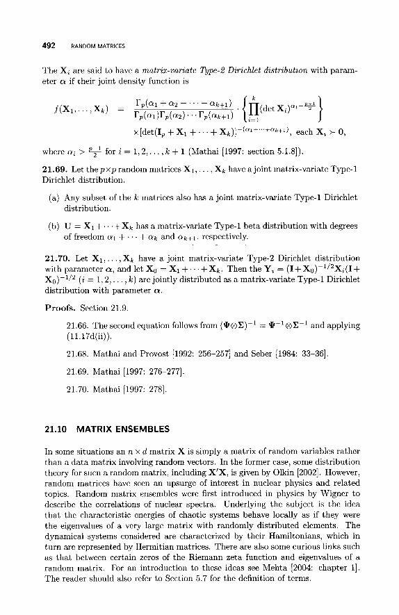
492 RANDOM MATRICES
The Xi are said to have a matrix-variate Type-2 Dirichlet distribution with param- eter a if their joint density function is
x [det(I, + X1 + . . . + X ~ , ) ] - ( ~ l + . " + ~ ~ + l ) , each X, + 0,
where a, > 9 for i = 1,2, . . . , k + 1 (Mathai [1997: section 5.1.81).
21.69. Let t h e p x p random matrices XI , . . . , Xk have ajoint matrix-variate Type-1 Dirichlet distribution.
(a) Any subset of the k matrices also has a joint matrix-variate Type-1 Dirichlet distribution.
(b) U = X1 +. . . +XI, has a matrix-variate Type-1 beta distribution with degrees of freedom a1 + . . . + a k and a1,+1, respectively.
21.70. Let X1, . . . , XI, have a joint matrix-variate Type-2 Dirichlet distribution with parameter a, and let XO = X1+. . .+Xk . Then t h e y , = ( I + X O ) - ~ / ~ X , ( I + Xo)-1/2 ( i = 1 ,2 , . . . , k ) are jointly distributed as a matrix-variate Type-1 Dirichlet distribution with parameter a.
Proofs. Section 21.9.
21.66. The second equation follows from (@@E)-' = @-'@E-' and applying ( ll .l7d(ii)).
21.68. Mathai and Provost [1992: 256-2571 and Seber [1984: 33-36].
21.69. Mathai [1997: 276-2771.
21.70. Mathai [1997: 2781.
21.10 MATRIX ENSEMBLES
In some situations an n x d matrix X is simply a matrix of random variables rather than a data matrix involving random vectors. In the former case, some distribution theory for sucn a random matrix, including X'X, is given by Olkin [2002]. However, random matrices have seen an upsurge of interest in nuclear physics and related topics. Random matrix ensembles were first introduced in physics by Wigner to describe the correlations of nuclear spectra. Underlying the subject is the idea that the characteristic energies of chaotic systems behave locally as if they were the eigenvalues of a very large matrix with randomly distributed elements. The dynamical systems considered are characterized by their Hamiltonians, which in turn are represented by Hermitian matrices. There are also some curious links such as that between certain zeros of the Riemann zeta function and eigenvalues of a random matrix. For an introduction to these ideas see Mehta [2004: chapter I]. The reader should also refer to Section 5.7 for the definition of terms.
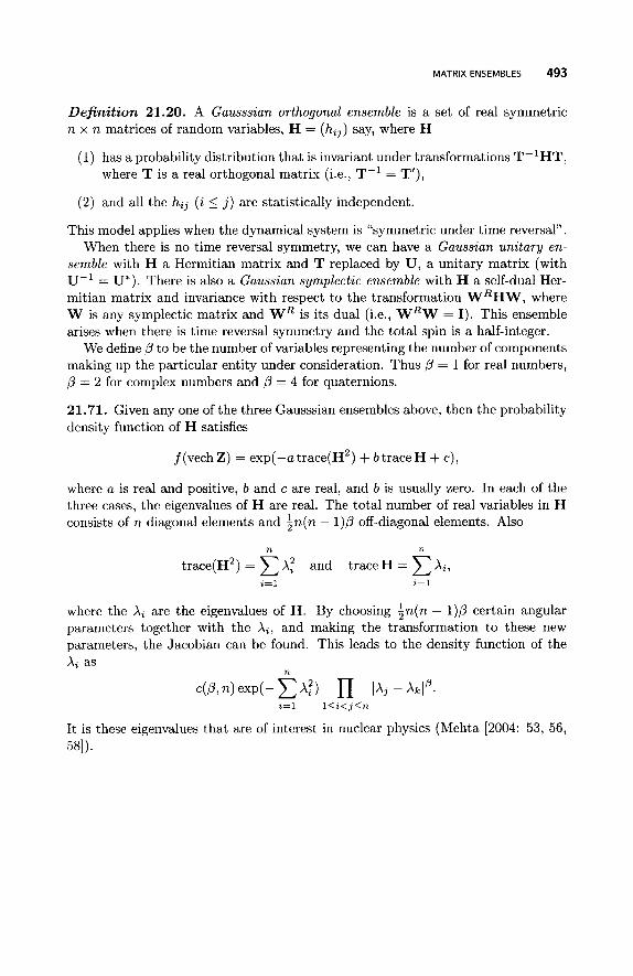
MATRIX ENSEMBLES 493
Dejki t ion 21.20. A Gausssian orthogonal ensemble is a set of real symmetric n x n matrices of random variables, H = (hz3) say, where H
(1) has a probability distribution that is invariant under transformations T-’HT, where T is a real orthogonal matrix (i.e., T - I = T’),
(2) and all the h,, ( i 5 j ) are statistically independent.
This model applies when the dynamical system is “symmetric under time reversal”. When there is no time reversal symmetry, we can have a Gaussian unitary en-
semble with H a Hermitian matrix and T replaced by U, a unitary matrix (with U-’ = U*). There is also a Gaussian symplectic ensemble with H a self-dual Her- mitian matrix and invariance with respect to the transformation WRHW, where W is any symplectic matrix and WR is its dual ( ie . , WRW = I). This ensemble arises when there is time reversal symmetry and the total spin is a half-integer.
We define p to be the number of variables representing the number of components making up the particular entity under consideration. Thus p = 1 for real numbers, p = 2 for complex numbers and p = 4 for quaternions.
21.71. Given any one of the three Gausssian ensembles above, then the probability density function of H satisfies
f(vechZ) = exp(-atrace(H2) + btraceH + c ) ,
where a is real and positive, b and c are real, and b is usually zero. In each of the three cases, the eigenvalues of H are real. The total number of real variables in H consists of n diagonal elements and in(n - l)p off-diagonal elements. Also
n n
trace(H2) = c A: and trace H = c A,,
where the A, are the eigenvalues of H. By choosing in (n - l)p certain angular parameters together with the A,, and making the transformation to these new parameters, the Jacobian can be found. This leads to the density function of the A, as
a=1 ,= 1
n
It is these eigenvalues that are of interest in nuclear physics (Mehta [2004: 53, 56,
581).

This Page Intentionally Left Blank
CHAPTER 22
INEQUALITIES FOR PROBABILITIES AND RANDOM VARIABLES
Inequalities arise in many places in probability and statistics. For example, Tong [1980: chapter 81 gives a number of applications of probability inequalities to si- multaneous confidence regions, hypothesis testing and simultaneous comparisons, ranking and selection problems, and reliability and life testing. Some of the re- sults in this chapter can be proved using the concept of majorization and Schur convexity, discussed in Chapter 23.
22.1 GENERAL PROBABILITIES
Let E, (i = 1 , 2 , . . . , n) be any events.
22.1. (Boole’s Formula)
From this we can derive the following inequalities: n
i= 1
A Matrix Handbook for Statisticians. By George A. F. Seber Copyright @ 2008 John Wiley & Sons, Inc.
495
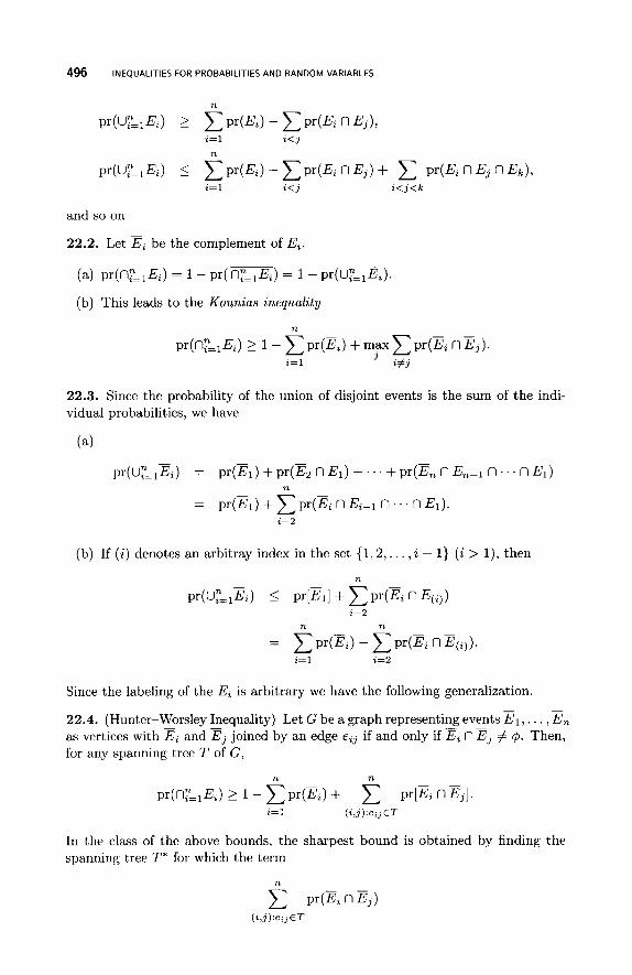
496 INEQUALITIES FOR PROBABILITIES AND RANDOM VARIABLES
i=l i<j
n
and so on
22.2. Let Ei be the complement of Ei. -
(a) pr(nr=lEi) = 1 - pr( n;=lEi) = 1 - pr(UY=,Ei).
(b) This leads to the Kounias inequality
n
22.3. Since the probability of the union of disjoint events is the sum of the indi- vidual probabilities, we have
(4 pr(U~==,E,) = pr(E1) + pr(E2 n E ~ ) + . . . + pr(En n
= pr(E1) + C p r ( E , n E ~ - ~ n . . . n E ~ ) .
n . . . n ~ 1 )
n
i=2
(b) If ( i ) denotes an arbitray index in the set {1,2,. . . , i - l} ( i > l), then
n
pr(UyT1Ei) I pr[E11 + C ~4% n ~ ( i ) )
i=2 n n
i=l i=2
Since the labeling of the Ei is arbitrary we have the following generalization.
22.4. (Hunter-Worsley Inequality) Let G be a graph representing events El,. . . , En as vertices with Ei and E j joined by an edge eij if and only if Ei nE, # 4. Then, for any spanning tree T of G,
-
n n
In the class of the above bounds, the sharpest bound is obtained by finding the spanning tree T' for which the term
n
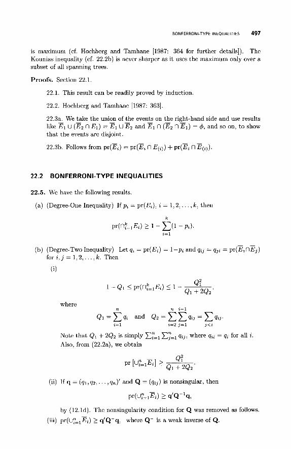
BONFERRONI-TYPE INEQUALITIES 497
is maximum (cf. Hochberg and Tamhane [1987: 364 for further details]). The Kounias inequality (cf. 22.2b) is never sharper as it uses the maximum only over a subset of all spanning trees.
Proofs. Section 22.1.
22.1. This result can be readily proved by induction.
22.2. Hochberg and Tamhane [1987: 3631.
22.3a. We take the union of the events on the right-hand side and use results like El U (Ez n E l ) = El U F2 and El n (Ez n El) = 4, and so on, t o show that the events are disjoint.
22.3b. Follows from pr(Ei) = pr(Ei n E(i)) + pr(Ei n E(i)) .
22.2 BONFERRONCTYPE INEQUALITIES
22.5. We have the following results.
(a) (Degree-One Inequality) If p , = pr(Ei), i = 1 ,2 , . . . , k , then
k k Pr(n,=,EJ 2 1 - C ( 1 - Pz).
2=1
- _ _ (b) (Degree-Two Inequality) Let yi = pr(Ei) = 1-pi and yij = yji = pr (E inEj )
for i , j = 1 , 2 , . . . , k. Then
6)
where n n 2-1
Note that Q1 + 2Q2 is simply Cy=l Cy=, yij, where yii = qi for all i. Also, from (22.2a), we obtain
(ii) If q = (41, y2 , . . . , yn)’ and Q = (y i j ) is nonsingular, then
pr(U:==,Ei) 2 q’Q-lq,
by (12.1d). The nonsingularity condition for Q was removed as follows. -
(iii) pr(U;==,Ei) 2 q’Q-q, where Q- is a weak inverse of Q.
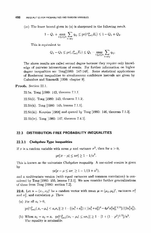
498 INEQUALITIES FOR PROBABILITIES AND RANDOM VARIABLES
(iv) The lower bound given in (a) is sharpened in the following result.
Qi + Q2.
This is equivalent to
Qi - Q Z I ~r(Ur=iEi ) I Qi - ly~2n C qij. i : i # j
The above results are called second degree because they require only knowl- edge of pairwise intersections of events. For further information on higher degree inequalities see Tong[1980: 147-1481, Some statistical applications of Bonferroni inequalities to simultaneous confidence inervals are given by Galambos and Simonelli [1996: chapter 81.
Proofs. Section 22.1.
22.5a. Tong [1980: 143, theorem 7.1.11
22.5b(i). Tong [1980: 143, theorem 7.1.21.
22.5b(ii). Tong [1980: 145, lemma 7.1.11.
22.5b(iii). Kounias [1968] and quoted by Tong [1980: 146, theorem 7.1.31.
22.5b(iv). Tong [1980: 147, theorem 7.4.11.
22.3 DISTRIBUTION-FREE PROBABILITY INEQUALITIES
22.3.1 Chebyshev-Type Inequalities
If x is a random variable with mean p and variance a’, then for a > 0,
pr[lz - p~ I U(T] 2 1 - 1 /2 .
This is known a s the univariate Chebyshev inequality. A one-sided version is given
bY pr[z - p 5 aa] L 1 - 1/(1+ a’),
and a multivariate version (with equal variances and common correlation) is con- sidered by Tong [1980: 155, lemma 7.2.11. We now consider further generalizations of these from Tong [1980: section 7.21.
22.6. Let x = (51, z2)’ be a random vector with mean p = ( p i , pz)’, variances a! and 02, and correlation p . Then:
(a) For all a, > 0,
2 2 2 i f 2 pr[n,2_1(Ix,-p,I I w,)] 2 1 - { ( a ~ + a ~ ) + [ ( a ~ + a ~ ) 2 - 4 4 p a l G ) / ( 2 4 4 ) .
2 112 (b) When a1 = a2 = a, pr[n?=’=,(lx, - p21 5 aa,)] 2 1 - [l + (1 - p ) ]/a2. The equality is attainable.
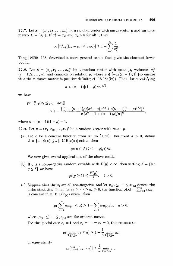
DISTRIBUTION-FREE PROBABILITY INEQUALITIES 499
22.7. Let x = (21, x2,. . . , xn)' be a random vector with mean vector p and variance matrix C = (ai j) . If a: = aii and ai > 0 for all i, then
Tong [1980: 1531 described a more general result that gives the sharpest lower bound.
22.8. Let x = (xl , 2 2 , . . . , zn)' be a random vector with mean p, variances a: (i = 1 , 2 , . . . , n), and common correlation p, where p E [-l/(n - l ) , 11 (to ensure that the variance matrix is positive definite; cf. 15.18a(iv)). Then, for a satisfying
a > (n - 1)[(1- p)/n]1/2,
we have
{[(1+ (n - l)p)(a2 - u)]1/2 + a ( n - 1)(1- p)1/2}2
n{a2 + [l + (n - l)p]/n}2 21- ,
where u = (n - 1)(1 - p) - 1.
22.9. Let x = ( ~ 1 ~ x 2 , . . . , xn)' be a random vector with mean p.
(a) Let q5 be a concave function from Rn to [0,00). For fixed a > 0, define A = {x I d(x) I a} . If E[+(x)] exists, then
pr(x E A ) 2 1 - +(p) /a ,
We now give several applications of the above result.
(b) If y is a non-negative random variable with E(y ) < 00, then setting A = {y : y 5 6) we have
E(Y) pr(y 2 6) 5 -, 6 > 0.
6
(c) Suppose that the xi are all non-negative, and let 5 . . . 5 x ( ~ ) denote the order statistics. Then, for c1 2 . . . 2 cn 2 0, the function +(x) = cyzl ciz(,) is concave in x. If E ( x ( ~ ) ) exists, then
n n
i= 1 i = l
where p(l) 5 . . . 5 p ( n ) are the ordered means.
For the special case c1 = 1 and c2 = .. . = c, = 0, this reduces to
or equivalently
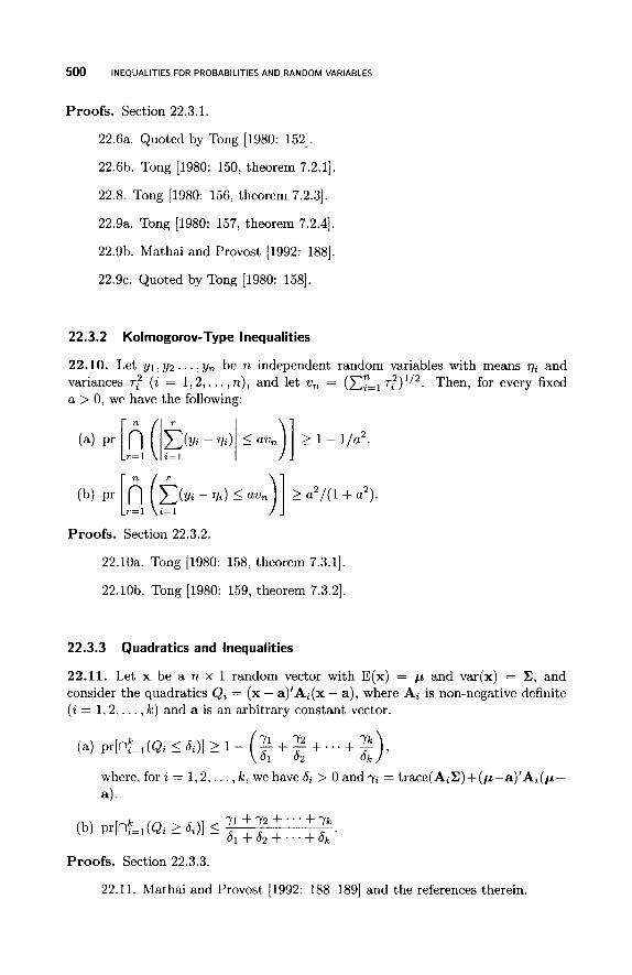
500 INEQUALITIES FOR PROBABILITIES AND RANDOM VARIABLES
Proofs. Section 22.3.1.
22.6a. Quoted by Tong [1980: 1521.
22.613. Tong [1980: 150, theorem 7.2.11.
22.8. Tong [1980: 156, theorem 7.2.31.
22.9a. Tong [1980: 157, theorem 7.2.41.
22.9b. Mathai and Provost [1992: 1881.
22.9~. Quoted by Tong [1980: 1581.
22.3.2 Kolmogorov-Type Inequalities
22.10. Let y1, yz . . . , yn be n independent random variables with means rli and variances 7: (i = 1 , 2 , . . . , n) , and let wn = ( C z , T : ) ~ / ' . Then, for every fixed a > 0, we have the following:
Proofs. Section 22.3.2.
22.10a. Tong [1980: 158, theorem 7.3.11.
22.10b. Tong [1980: 159, theorem 7.3.21.
22.3.3 Quadratics and Inequalities
22.11. Let x be a n x 1 random vector with E(x) = p and var(x) = E, and consider the quadratics Qi = ( x - a)'Ai(x - a) , where Ai is non-negative definite (i = 1,2, . . . , k) and a is an arbitrary constant vector.
where, for i = 1 , 2 , . . . , k , we have 6i > 0 and yi = trace(AiE)+(p-a)'Ai(p-
a).
Proofs. Section 22.3.3.
22.11. Mathai and Provost [1992: 188-1891 and the references therein.
DATA INEQUALITIES 501
22.4 DATA INEQUALITIES
22.12. The following inequalities hold for any numbers, but the main application is to random observations.
(a) Let x1 ,x2 , . . . ,x, be n observations and define ?t = C:=l xi/. and i?’ = Cy=l (xi - :)2/n. Then
( X i - c)2 I (n - 1 ) 2 , i = 1 , 2 , . . . ,n.
Equality holds if all the other xj’s are equal except xi. For an extension of the above see Kabe [1980].
(b) Let x1 2 22 2 . . . 2 2,. Then
. - . A x - oJ(r~ - l ) ) / (n - r~ + 1) 5 x k I T + z J ~ . Equality occurs on the left-hand side if and only if
x k - 1 and X k = xk+l 1 .. ’ = X n, x1 = x2 = . . . =
and on the right-hand side if and only if
= x2 = . . . = x k and xk+l = xk+2 = . . . = 2,.
(c) Suppose xl, x2,. . . , x, are &dimensional observations. Let X, = cy=l xi/n and S, = xi - X,)(X~ - X,)‘/n. Then
(n - 1)S, - (xj - %,)(xj - %,)I is non-negative definite,
or equivalently,
(x. 3 -xn)’S;1(xj -q I n - 1, j = 1 , 2 , . . . ,n.
Thus each xj lies in the interior or on the surface of the ellipsoid (x - x,)’S;l(x - x,) = n - 1. If S, is singular, we can replace S i l by S;, a weak inverse of S,.
(d) If X(j) = Ci:izj xi, then
n2 -S, - (xj - %i(j)(xj - Xcj ) ) ’ n - 1
or equivalently,
is non-negative definite,
Proofs. Section 22.4.
22.12a. Isotalo et al. [2005b: 1761 and Samuelson [1968].
22.1213. Farnum [1989] and Wolkowicz and Styan [1979].
2 2 . 1 2 ~ . Trenkler and Puntanen [2005]
22.12d. Trenkler and Puntanen [2005].
502 INEQUALITIES FOR PROBABILITIES AND RANDOM VARIABLES
2 2.5 I N E Q U A L I T I ES FOR EX P ECTAT I 0 N S
22.13. (Multivariate Jensen's Inequality) Let x be an n x 1 random vector with finite expectation E(x) = p.
(a) Let 4 be a real-valued convex function defined on S , where S is a convex subset of R". If pr(x E S) = 1, then
(b) If 4 is a symmetric (cf. Definition 23.6 above (23.14)) and continuous function on R", then
where ~ ( 1 ) 2 ~ ( 2 ) 2 . . . 2 P ( ~ ) and ~ ( 1 ) 2 q 2 ) 2 . . . 2 qn). 4 ( P ( l ) , P ( 2 ) , . . . , P ( " ) ) 5 E [ 4 ( ~ ( 1 ) , ~ ( 2 ) , ' . . , ~ ( " , ) 1 ,
22.14. (Finite Population) Suppose that zl, zg, . . . ,z, are obtained by sampling without replacement from a finite population, and y1, yg, . . . , yn are obtained by sampling with replacement from the same population. Then if g is continuous and convex.
Proofs. Section 22.5.
22.13. Schott [2005: 3781
22.14. Hoeffding [1963] and quoted by Marshall and Olkin (1979: 331-3431.
22.6 M U LTI VA R I ATE I N EQ U ALlT I ES
22.6.1 Convex Subsets
22.15. Let x E Rd be a random vector with symmetric probability density function f(x),that is, f(-x) = f (x) , such that the set {x : f(x) 2 a } is convex for all a > 0. Suppose that S is a convex subset of Rd and is symmetric about 0 (i.e., if x E S then -x E S also). Then:
(a) pr(x + cb E S ) 2 pr(x f b E S ) for any constant b E S and 0 5 c 5 1.
(b) The result (a) still hold if b is replaced by y, a random vector distributed independently of x.
(c) If x N N d ( O , X ) , then its probability density function satisfies the above conditions.
(d) If x - Nd(0, X I ) and y - Nd(0, Eg), where El - Eg is non-negative definite, then pr(x E S ) 5 pr(y E S ) . This type of result has been extended to elliptically contoured distributions by Perlman [1993].
Many of the unimodal symmetric multivariate distributions centered at the origin, like the multivariate normal and multivariate t-distribution, satisfy the conditions of this theorem. For further background see Anderson 119961.
MULTIVARIATE INEQUALITIES 503
22.6.2 Multivariate Normal
22.16. (Slepian Inequality) Suppose x N Nd(0, C), where C = (aij) is non-negative definite. Let yi = xi/&, i = 1,2, . . . , d so that y N N,j(O, R), where R = ( p i j ) is the population correlation matrix. Then, for any constants c1, c2,. . . , c d ,
is an increasing function for each pi j , i # j. If R is positive definite, then the above is a strictly increasing function of p i j , i # j.
Replacing ci by &cir we see that the result still holds if use the zi instead of the yi.
If all the pij 2 0 ( i # j ) , then
d
If pij 5 0 for all i, j , i # j, the above inequality is reversed. Because we can transform from zi t o yi, researchers have focused, without any
loss of generality, on deriving results for y, where y N Nd(0,R) and R is the correlation matrix.
22.17. (Khatri)
(a) Suppose x = (xil), xt2))’ N N d ( 0 , C), where x ( k ) is dk x 1 ( k = 1,2) and d = dl + d2. Let
C = ( ;;; ;;; ) , where !&k is dk x dk. Let A1 C &tdl and A2 C &tdZ be two convex regions that are symmetric about the origin (cf. 22.15). If El2 has rank zero (i.e.,
= 0) or has rank one, then
2
pr [n:=l(X(k) E Ak)] 2 n Pr(X(k) E Ak). k=l
Setting x ( ~ ) = 5 1 , we have
pr(lz1l I U l , X ( 2 ) E A2) 2 pr(lz1l I adPr(X(2) E A2),
and repeatedly applying this result to each element of ~ ( 2 ) ~ we obtain
d
pr [ n L ( l z i l I ai)] 2 ~ [ P ~ ( I Z ~ I I ai ) . i=l
This inequality is strict if C is positive definite, C is not a diagonal matrix, and all the ais are positive.
The above results have been generalized to the case when the mean of x is not necessarily zero. For details see Tong [1980: theorem 2.2.31.
If the correlation matrix R of x has structure 1 (see (b) below) and is positive definite, then C12 has rank 0 or 1 (quoted by Tong [1980: 33, example 111).
504 INEQUALITIES FOR PROBABILITIES AND RANDOM VARIABLES
(b) Suppose x = ( x i l ) , x i2) , . . . , xiT))’, where x N Nd(0, R) and R = ( p z j ) is the
correlation matrix. Here x ( k ) is d k x 1 (k = 1 , 2 , . . . , r ) , where d k = d. For each k, let A k c Rdk be a convex region symmetric about the origin. Suppose we have the product structure p i j = A&, X i E ( - l , l ) , for all i , j ( j # i), called structure 1 by Tong, then the following inequalities hold.
(i) Firstly,
Pr [ n ; , l ( x ( k ) E Ak)] 2 Pr [ k C ( X ( k ) E A k ) ]
x Pr [ n k @ C ( x ( k ) E Ak)] T
2 k=l
and
2 n PT(X(L) 4. A k ) k = l
holds for every subset C of the integers { 1 , 2 , . . . , r } . The inequalities are strict if the Ai’s are bounded sets with positive probabilities and the Xi’s are nonzero.
(ii) We then have the following special case of the above.
d
pr [ n $ l ( I Z i I 2 ai)] 2 H P ~ ( I ~ ~ I 2 ail. i = l
22.18. (Sid&k’s Theorem) Let x - Nd(0, R(X), where R(X) = ( p i j ( X ) ) is a correla- tion matrix depending on X 6 [0,1] in the following way: For a fixed non-negative definite correlation matrix T = (qj), we define p i j ( X ) = ~ i j for all i, j = 2 , 3 , . . . , d and p l , ( X ) = p j l ( X ) = X ~ 1 j for j = 2, . . . , d. Then R(X) is non-negative definite for X E [0, I], and
is monotonically nondecreasing in X E [0,1] for every ai (i = 1 , 2 , . . . , d) . If T is positive definite (which implies R(X) is positive definite), r1j # 0 for some j > 1, and all the ais are positive, then the above probability is strictly increasing in A.
A consequence of the above result is that if we now have correlation matrix R(X), where X = ( X I , Xz,. . . , A d ) ’ , p i j ( X ) = X i X j ~ i j for all z # j , and each X i E [0,1], then the above probability is monotonically nondecreasing in each X i E [0, I]. It is strictly increasing in Xi if T = (r,j) is positive definite, X i ~ i ~ i j # 0 for some j # i, and all the ais are positive.
22.19. Suppose x N N d ( o , x ) , where a i j = a’ for z = j , aij = p a 2 for a # j , and p E [0,1]. Define for k = 1 , 2 , , . . , d and a > 0,
Pr [nL&zl 5 .i)]
~ r , ( k ) = pr [ n L l ( Z i I a ) ]
ply($\ = p r L ~ & ~ ( ~ ~ i ~ - < ~ ) l
MULTIVARIATE INEQUALITIES 505
and k
pr,(k) = Pr [n,=,(lx,l 2 43 .
pr,(d) L [pr,(k)Pk L [pr,(1)ld, d > 2 2.
Then, for m = 1,2,3, we have
The inequalities are strict if p > 0.
Definition 22.1. Let x = (x1,x2, . . . ,xd)' be a random vector. We say that the elements of x are assoczated random vamables if for any two univariate functions g,(x) of x such that E[g,(x)] exists (z = 1,2) that are nondecreasing in each ar- gument, we have cov[gl(x),g2(x)] 2 0. Esary et al. [1967], who introduced the concept, have given a number of results that can be used to readily verify that a given set of random variables is associated.
22.20. The following statements are true.
(a) Any subset of associated random variables is a set of associated random vari- ables.
(b) The set consisting of a single random variable is associated.
(c) If two sets of associated random variables are independent, then their union is a set of associated random variables.
(d) Independent random variables are associated.
(e) Nondecreasing functions of associated random variables are associated ran-
22.21. If the elements of the d x 1 vector x are associated random variables, then
dom variables.
d pr [nz=1(x2 I a,)] L pr [ n E ~ ( x , I a,)] pr [n,&z I 41
d
L H p r ( x , I a,) z= 1
holds for all a, and all subsets C of { 1 , 2 , . . . , d }
Proofs. Section 22.6.2.
22.15. Results quoted by Schott [2005: 83, exercise 2.611 and follow from (2.65e).
22.16. Tong [1980: section 2.11.
22.17a. Tong [1980: 16-19].
22.17b(i). Quoted by Hochberg and Tamhane [1987: 3671 and proved by Tong [1980: theorems 2.2.4 and 2.3.21.
22.17b(ii). Tong [1980: 28, theorem 2.3.31.
22.18. Tong [1980: 21, theorem 2.2.5, corollary 11.
22.19. Tong [1980: 30, theorem 2.3.41.
22.20. Tong [1980: 87, theorem 5.2.21.
22.21. Tong [1980: 89, theorem 5.2.41.
506 INEQUALITIES FOR PROBABILITIES AND RANDOM VARIABLES
22.6.3 Inequalities For Other Distributions
22.22. (Multivariate &Distribution) Let x = ( X I , 2 2 , . . . , x d ) ’ N Nd(0, R), where we can assume without loss of generality that R = ( p i j ) is the correlation ma- trix with p,i = 1 (cf. 22.16). Let z, = xilu, where u is distributed as a random variable independent of x. Then z = (z1, z2 , . . . , zd)’ has a multivariate t-distribution with Y degrees of freedom and associated correlation matrix R. In terms of the notation of Section 20.8.1, y N t d ( Y , 0, R).
By conditioning on u, the following inequalities from above still hold with xi or yi replaced by zi.
(a) If all the p i j 2 0, then
(b) pr [nf==l((zil I ai)] L &l pr(Izi1 I ai).
This inequality is strict if R is positive definite, R is not a diagonal matrix, and all the ais are positive.
(c) If p i j = X i X j (all i , j , j # i), where each X i E ( - l ,+ l ) , then
d
pr [nt==l(Izil 2 4 2 n p r ( b i l 2 ail. i=l
22.23. (Correlated F-ratios) Let xg, x:, . . . , xE be independent chi-square vari- ables with degrees of freedoom Y O , v 1 , . . . V k , and let Fi = ( X ~ / V ~ ) / ( ~ ~ / Y O ) , i = 1 , 2 , . . . ,k. Then
k
i=l
k
(b) pr [&,(Fi > ai)] > n ~ r ( F i > ai). a= 1
Proofs. Section 22.6.3.
22.22. Hochberg and Tamhane [1987: 3691.
22.23. Tong [1980: 43, theorem 3.2.21.
CHAPTER 23
M A J 0 R I Z AT I 0 N
Majorization does not seem to be a topic very well known in statistical circles. However, majorization can be used to prove a number of inequalities. A key result is (23.7), from which we may assume without any loss of generality (Tong [1980: 1051) that only two coordinates need be different when proving inequalities. Two applications are, for example, species-diversity indices (Tong [1983]) and optimal design theory (Bhaumik [1995]). The topic is also relevant to the finding of optimal statistical tests (Anderson [2003: section 8.101).
23.1 GENERAL PROPERTIES
Definition 23.1. Let x = ( q , x 2 , . . . , zn)' and y = (yi, y ~ , . . . ,yn)' be vectors in R". Suppose the zi are ordered in decreasing order of magnitude as 2 ~ ( 2 ) 2 . . . 2 "("1, with the yi ordered in a similar fashion. We say that x is (strongly) majorized by y (or y majorizes x), and use the symbol x << y (or y >> x), if
Z(1) + Z(2 ) + ' ' ' + X ( i ) I Y(1) + Y(2) + ' ' . + Y ( i ) , 2 = 1,2, . . . , n - 1,
Z l + Z 2 + . . . + 2 , = y1+yz+. . .+y n.
This definition is given by Marshall and Olkin [1979] and Horn and Johnson [1991], except they use qi] instead of Z C ( ~ ) . They and most other authors, except Rao and Rao [1998: chapter 91, use x 3 y instead of x << y; however, I have reserved the
A Matrix Handbook for Statisticians. By George A. F. Seber Copyright @ 2008 John Wiley & Sons, Inc.
507
508 MAJORIZATION
former symbol in the form of A + 0 for positive definite matrices and used A > 0 for matrices with all positive elements.
The above definition has also been exended to infinite sequences (Marshall and Olkin [1979: 161) and to random vectors (Marshall and Olkin [1979: chapter 111).
23.1. If the x, (and the yz) are ordered in increasing magnitude, say x{l} 5 x{2} 5 . . . 5 xtn}, then since = x(n-z+l), x << y if and only if
5{1} + X { 2 } + . . . + X { 2 } 2 Y{1} +Y{2} + . . . + y{%}, 2 = 1 , 2 , . . . , n - 1,
2 1 + 2 2 + . . . + x , = y 1 + y 2 + . . . + y n.
Some authors use this result as their definition, which I find confusing because of the direction of the inequalities. Using the notation 3+1 instead of x ~ ( ~ } , Rao and Rao [1998: 3041 proved the equivalence of the two definitions.
23.2. Let 7r be a permutation of {1,2,. . . , n}. If x, y, and z are in R”, and x, is the vector whose components are a permutation of the elements of x, then the following hold.
(a) x << x.
(b) If z = Cy=, x,/n, then Zln << x.
(c) x << x, for every permutation T .
(d) If x << y and y << z, then x << z.
(c) If x << y and y << x, then y = x, for some permutation T .
( e ) If x << z, y << z, and 0 5 a 5 I, then ax + (I - a ) y << z. ( f ) If x << y, x << z, and 0 5 a 5 I, then x << a y + (1 - a)z .
(g) If z is any vector, then
(:) << (:) if and only if x << y.
23.3. The following conditions are equivalent.
(I) x < y .
(2) x = Ay for some doubly stochastic matrix A
(3) x = By for some orthostochastic matrix B.
Note that A and B are not unique.
GENERAL PROPERTIES 509
23.4. If x 2 0, y 2 0, and x << y, then nl", zi 2 ny=l yi.
23.5. (Schur) If H be an n x n Hermitian matrix with (real) eigenvalues given by the vector X(H) = (X1,X2,. . . ,A,)', where X1 2 . . . 2 A,, and (real) diagonal elements h = (h l l , h 2 2 , . . . h",)', then
h << X(H)
on R". This result is an example of a number of inequalities involving the eigen- values and singular values of a matrix (cf. Marshall and Olkin [1979: chapter 9]), some of which are quoted elsewhere.
23.6. (Fan) If A and B are n x n Hermitian matrices, then
X(A + B) << X(A) + X(B).
Definition 23.2. If Q is a permutation matrix that interchanges just two coor- dinates of a vector x (say xj and xk), then a T-transform, denoted by Tx, has T of the form T = X I + (1 - X)Q, where 0 5 X I 1. What Tx does is transform xj into Xxj + (1 - X ) x k and zk into Xxk + (1 - X)zj, leaving the other elements of x unchanged. For example, if Q interchanges the first two elements of x E R", then Q = ( e 2 , e l , . . . , en) is I, with its first two columns interchanged.
23.7. We have x << y if and only if there exists a finite number of real vectors c1, c2,. . . c, such that x = c1 << c:! << . . . << c,-1 << c, = y, where, for all i, ci and ci+l differ in two coordinates only. Thus if x << y, then y can be derived from x by successive applications of a finite number of T-transforms.
Definition 23.3. (Weak Majorization) We now generalize the Definition 23.1 above. A vector x is said to be weakly (sub)majorized by y, and we denote the relationship by x <<w y, if
x(1) + " ( 2 ) + . . . + z(i) I y(1) + Y ( ~ ) + . . . + y(%), i = 1 ,2 , . . . ,n.
Marshall and Olkin [1979] use the notation x 4" y for weak (sub)majorization. Some authors omit the prefix "sub".
We say that x is weakly (super)majorized by y and denote the relationship by x <<lU y if
z{,} + z{2} + . . . + z{q 2 y{1) + y12) + . . . + qi), i = 1 ,2 , . . . , n.
23.8. The results below follow directly from the previous definitions.
(a) x <<" y if and only if -x KW -y.
(b) x <<w y and x <<" y if and only if x << y.
(c) x 5 y (i.e., z, 5 yi for all i) implies that x eW y and x >" y.
(d) x <<w y if and only if for some u, x 5 u and u << y.
(e) x <<I" y if and only if for some v, x << v and v 2 y.
510 MAJORIZATION
23.9. Let R+ = [ O , c o ) . Then x KW y on R; if and only if there exists a doubly stochastic matrix A such that x = Ay.
23.10. x <<W y if and only if Cy=l q5(x:i) 5 q5(yi) for all continuous monotonically increasing convex functions q5 (cf. Definition 23.5 below).
23.11. Let A and B be n x n symmetric matrices, and suppose that X,(C) 2 X2(C) 2 . . . 2 X,(C) with X(C) the corresponding vector, where C = A or B. Then
X(A + B)) eW X(A) + X(B.
23.12. If A and B are n x n matrices and A 5 B (i.e., aij 5 bij for all i . j ) , then using the notation of (23.11) above we have
23.13. Let A and B be n x n real or complex matrices, and let o l ( C ) 2 o2(C) 2 . . . 2 ok(C) ( k = min{m, n}) , with u(C) the corresponding vector. Then:
(a) a(A + B) <<W a(A) + a(B). (b) If m = n,
( i ) a(AB) <<, cr(A) 0 u(B).
(ii) a(A o B) << a(A) o a(B)
Here “0” is the Hadamard product.
Proofs. Section 23.1
23.2. Rao and Rao [1998: 303-307, for (a)-(g)] and Marshall and Olkin [1979: 7, for (h)].
23.3. Marshall and Olkin [1979: 21-24].
23.4. Quoted by Rao and Rao [1998: 3201.
23.5. Marshall and Olkin and Olkin [1979: 2181 and Zhang [1998: 2301.
23.6. Marshall and Olkin [1979: 2411 and Zhang [1999: 2311.
23.7. Marshall and Olkin [1979: 211 and Rao and Rao [1998: 3161
23.8. Marshall and Olkin [1979: 111.
23.9. Horn and Johnson [1991: 166-1671.
23.11. Anderson [2003: 3571.
23.12. Anderson [2003: 3591.
23.13. Zhang [1998: 2321.
SCHUR CONVEXITY 511
23.2 SCHUR CONVEXITY
Definition 23.4. Let f be a function from R" to R" (m > 1) defined on A c R". Then f is said to be Schur-convex on A if
x,y E R" and x << y on A * f(x) KW f(y).
Also f is said to be strongly Schur-convex on A if
x, y E R" and x <<, y on A + f(x) KW f(y),
and f is said to be strictly Schur-convex on A if
x,y E R" and x << y on A + f(x) << f(y).
If A = R", we drop the words "on A". Note that the label "schur-convex" is a bit misleading as such a function is not necessarily convex.
A function f is Schur-concave if (-f) is Schur-convex. (The above definitions come from Rao and Rao [1998: 3071, except m and n are interchanged.)
The above definitions need to be clarified as follows when m = 1 and f is no longer a vector (say 4 ) . The function 4 is Schur-convex (respectively concave) on A if x, y E R" and x << y on A + 4(x) I @(y) (respectively 4(x) 2 4(y)). If y is not a permutation of x, then 4 is said to be strictly Schur-convex (respectively concave) on A if x,y E R" and x << y on A + 4(x) < 4(y) (respectively 4(x) > +(y)).
Schur convexity or concavity can be used to prove many inequalities. For ex- ample, Marshall and Olkin [1979: chapter 81 list a number of inequalities including those relating to the angles or sides of various geometrical figures such as triangles and polygons. Schur convexity also arises in combinatorial analysis, particularly with respect to graph theory, the theory of network flows, and the study of incidence matrices (Marshall and Olkin [1979: chapter 71).
Definition 23.5. Let f be a function from R" to R" (m > 1) defined on A c Rn, and let x I y (i.e., xi 5 yi for each 2) . Then f is said to be montonically increasing on A if x,y E R" and x 6 y on A + f(x) I f(y), monotonically decreasing if -f is monotonically increasing, and monotone if it is either monotonically increasing or decreasing.
We recall from Section 2.5 that f is convex if
f(ax + (1 - a)y) I crf(x) + (1 - a)f(y),
for every 0 5 a 5 1 and x,y E R"; f is concave if -f is convex.
Definition 23.6. Let f be a function from R" to R", and let y = f(x). Then f is said to be symmetric if, for every permutation T of { 1 ,2 , . . . , n} , there exists a permutation T' of { 1,2, . . . , m} such that f(x,) = y,/ for all x E R".
If m = 1, so that f = 4 , say, then 4 is symmetric if d(x,) = 4(x) for all T .
Examples of symmetric functions for n = 3 are d(x) = x1 + 2 2 + 2 3 , d(x) =
5 1 2 2 + 5 2 2 3 + 53x1, and 4(x) = 2122x3.
23.14. If a function f from R" to R" is convex and symmetric, then it is Schur- convex. In addition, if f is monotonically increasing, then f is strongly Schur- convex.
512 MAJORIZATION
23.15. Let g be a function from R to R, and define
f(x) = (g(~l)>g(~2),"',~(~n))'.
Then, from the previous result, we have the following.
(a) If g is convex, then f is Schur-convex.
(b) If g is a convex monotonically increasing function, then f is strongly Schur- convex.
(c) Taking g(z) = 1x1, g(z) = x2, and g(z) = max{z,O} = z+, respectively, we have
(i) x << y implies that 1x1 <<" IyI.
(ii) x << y, u, = z: and w, = y; implies that u <<" v.
(iii) x << y implies that x+ <<" y+.
23.16. The following symmetric convex functions are Schur-convex.
(a) d(x) = max, Iz,I.
(b) d(x) = (C:=l lzZl')''', T L 1.
23.17. (Sum)
(a) Let Z be an interval of R, and let g be a function from Z to R. If g is (strictly) convex on Z, then +(x) = Cy=, g(z,) is (strictly) Schur-convex on Z", as 4 is symmetric. In this case, x << y on Z implies that d(x) 5 d(y) (or $(x) < d(y) for strict convexity).
There is also a converse result. Suppose g is continuous on Z. If 4 is (strictly) Schur-convex on In, then g is (strictly) convex on Z.
(b) Combining the above, the inequality
n n
i = l i= 1
holds for all continuous convex functions g from R to R if and only if x << y. Also, the same inequality holds for all continuous increasing convex functions g if and only if x <<" y. It holds for continuous decreasing convex functions g if and only if x <<" y.
23.18. The following are examples of strictly convex functions.
(a) For a > 0, g(z) = [z + ( l / z ) la is strictly convex on (0,1]. For a 2 1, g is strictly convex on (0, co).
(b) - logz is strictly convex on (0, a).
(c) g(z) = 1/11: is strictly convex on (0, co).
PROBABILITIES AND RANDOM VARIABLES 513
In each case 4(x) = Cr=l g(zi) is strictly Schur-convex. If xi > 0 and crZl xi = 1, then n-ll, << x (by 23.210) and 4(nP1ln) 5 4(x). We can use this result to set up inequalities. For example, using (a),
23.19. (Product) Let g be a continuous non-negative function defined on an inter- val 1. Then 4(x) = ny=l g(zi) is (strictly) Schur-convex on 1" if and only if logg is (strictly) convex on 1. Since, by (23.2b), :1, << x, we can use this result to obtain various inequalities. For example, logP(z) is strictly convex on R++ = (0,m) so that #(x) = ny=l r(zi) is strictly Schur-convex on Rn++. Hence
n
i = l
For further details about Schur-convex or Schur-concave functions see Marshall and Olkin [1979: chapter 31. Proofs. Section 23.2.
23.14. Rao and Rao [1998: 3181.
23.15a. Marshall and Olkin [1979: 1151 and Rao and Rao [1998: 3191.
23.1510. Marshall Olkin [1979: 1161 and Rao and Rao [1998: 3191.
23.15~. Rao and Rao [1998: 3191.
23.16. Marshall and Olkin [1979: 961.
23.17a. Marshall and Olkin [1979: 64, 671.
23.1710. Marshall and Olkin [1979: 108-1091
23.18-23.19. Marshall and Olkin [1979: 70-73, 751
23.3 PROBABILITIES AND RANDOM VARIABLES
23.20. (Probabilities) For i = 1 ,2 , . . . , n, let p , = pr(E,), and let q, be the proba- bility that at least k of the events El , E2,. . . , En occurs.
(a) If p = (PI. . . . ,prL) ' and q = (91,. . . , qn)', then p << q.
(b) From (a) we have Cr=l~pz = Cy=, q, and n;="=,, 2 nr=, q 2 .
23.21. (Expectations) Let x = ( z 1 , ~ 2 , . . . ,z,)' be a random vector with finite expectation, and define a, = E(z,), ti, = a ( t ) , and b, = E ( Z ( ~ ) ) , where a(1) 2 a(2) 2 . . . 2 a(,) and z(l) 2 ~ ( ~ 1 2 . . . 2 "(,I. Then:
(a) a << b.
(b) a << b.
514 MAJORIZATION
23.22. (Eigenvalues) Let Z be a random Hermitian n x n matrix with eigenvalues XI (Z) 2 X2(Z) 2 . . . 2 X,(Z) (which are all real). Then
(Xl(E[ZI),.’. ,Xn(E[Z]))’ -K (E[Xl(Z)l,..’,E[X,(Z)l)’,
where the Xi(E[Z]) are the eigenvalues of E[Z], the expectation of Z.
23.23. (Singular Values) Let W be an m x n random complex matrix with singular values al(W) 2 . . . 2 ot(W), where t = min(m,n). Then
(01(E[ZI), . ’ f ,an(E[ZI))’ KZu (Ebl(Z)I , . ’ . 3 E[an(Z)l)’
Proofs. Section 23.2.
23.20. Marshall and Olkin [1979: 345-3471,
23.21a. Rao and Rao [1998: 3051.
23.21b. Marshall and Olkin [1979: 3481.
23.22. Marshall and Olkin [1979: 3551.
23.23. Marshall and Olkin [1979: 3571.
CHAPTER 24
OPTIMIZATION AND MATRIX A P P ROX I MAT I0 N
The subject of finding unconstrained or constrained maxima and minima of func- tions is an extensive one. Schott [2005: section 9.71 gives a helpful summary. We consider only a few basic results in this chapter.
24.1 STATIONARY VALUES
Definition 24.1. Let f : x + f (x) be a real-valued function defined on S , a subset of R". Then f has a local m a x i m u m at c if, for some 6 > 0, f ( c ) 2 f (x) for all x such that IIx - cllz < 6. It has a strict local m a x i m u m if f ( c ) > f (x) for all x # c such that IIx - cllz < 6. Also, f has a global (absolute) m a x i m u m at c if f ( c ) 2 f(x) for all x E S. The function f has a local minimum at c if - f has a local maximum at c , and a global (absolute) minimum at c if - f has a global maximum at c .
Let c be an interior point of S (cf. Definition 2.29 below (2.63)). Then there exists a b > 0 such that x E S for all x satisfying IIx - cllz < 6. Suppose f is
then any point c satisfying the above equation is called a stationary point. (Note that f ( c ) is also called a critical value of f at c . ) Such a point can be a local maximum, a local minimum, or a saddle point.
A Matrax Handbook for Statastacaans. By George A. F. Seber Copyright @ 2008 John Wiley & Sons, Inc.
515
516 OPTIMIZATION AND MATRIX APPROXIMATION
24.1. (Unconstrained Local Optimization) Let f be defined as in Definition 24.1 above, and suppose that f is twice differentiable at c , where c is an interior point of S. If c is a stationary value o f f and V2f(c) is the Hessian o f f a t c (cf. Section 17.11), then:
(a) f has a strict local minimum at c if 02f (c) is positive definite.
(b) f has a strict local maximum at c if -V2f(c) is positive definite (i.e., V2f(c) is negative definite).
(c) f has a saddle point at c if V2f(c) is neither positive definite nor negative definite, but is nonsingular.
(c) f may have a local minimum, a local maximum, or a saddlepoint at c if V 2 f ( c ) is singular.
24.2. Minimizing a function is equivalent to minimizing a monotonically increasing transformation of that function. This result is particularly useful in maximum likelihood estimation, which is discussed in Section 24.3.1 below.
24.3. (Method of Lagrange Multipliers for Constrained Optimization) We now give sufficient conditions for finding a strict local maximum or minimum of a real-valued function f defined on S C Rn subject to the vector of constraints g(x) = 0, where g = (g l rg2 , . . . ,gm)’ is m x 1 (m < n).
Let c be an interior point of S, let F(x, A) = f(x)+A’g(x), where A E Rm (called the Lagrange multiplier; some use -A), and suppose that the following conditions hold:
(1) f and g are twice differentiable at c .
(2) B = ag(x)/ax’ = (agz(x)/ax,) has full row rank m at x = c.
(3) x = c is a solution of g(x) = 0 and dF(x, A)/ax = 0 (for some A).
If A is V2f(x) - Czl X,V2g,(x) evaluated at x = c, then f has a strict local maximum at x = c, subject t o g(x) = 0, if
x’Ax < 0, for all x # 0 for which Bx = 0.
A similar result holds for a strict local minimum with the inequality x’Ax > 0 replacing x’Ax < 0. In practice, one can often just simply solve the equations dF(x, A)/ax = 0 and g(x) = 0 for x and A, and then use ad hoc methods to check the nature of the constrained stationary value without having to investigate A.
24.4. Assuming that the conditions of the previous result (24.3) hold, we now give some equivalent sufficient conditions for a strict local maximum or a strict local minimum to exist. Let A be a symmetric n x n matrix and B an m x n matrix of rank m. Let A,, be the leading principal T x r submatrix of A, and let B, be the m x r matrix obtained by deleting the last n - r columns of B. For r = 1 ,2 , . . . , n, define the (m + r ) x (m + r ) matrix A, as
USING CONVEX AND CONCAVE FUNCTIONS 517
If B,, is nonsingular (which can be achieved by rearranging the 2, variables in (24.3)), then x’Ax > 0 holds for all x # 0 satisfying Bx = 0 if and only if
(-l)m det AT > 0 for all T = m + 1,. . . , n.
Also, x’Ax < 0 holds for all x # 0 satisfying Bx = 0 if and only if
( - l ) T det AT > 0 for all T = m + 1,. . . , n.
Examples using the above theory are given by Schott [2005: 380-3811 and Magnus and Neudecker [1999: 1381.
24.5. (Global Optimization) Finding the global maximum or minimum is some- times best achieved by using the ideas of convex sets and functions, as seen in the following results.
(a) On a convex set, the set of points at which the minimum of a convex function is attained is convex, and any local minimum is a global minimum. The same is true for a concave function, except replacing minimum by maximum.
A strictly convex function attains a minimum at no more than one point of a convex set, and a stationary (critical) point is necessarily a minimum.
(b) On a compact convex set, the maximum of a convex function occurs a t an extreme point. The same is true for the minimum of a concave function.
We now focus on convex and concave functions
Proofs. Section 24.1.
24.1. Schott [2005: 371-372; he omits the word “strict”] and Magnus and Neudecker [1999: 122-1231,
24.2. Magnus and Neudecker [1999: 1291.
24.3. Magnus and Neudecker [1999: 135-1381 and quoted by Schott [2005: 379-3801,
24.4. Magnus and Neudecker [1999: 53-54, 1361.
24.5. Quoted by Horn and Johnson [1985: 5351
24.2 USING CONVEX AND CONCAVE FUNCTIONS
24.6. Let f : x + f(x) be a real-valued convex function defined on S , a convex subset of R”.
(a) Corresponding to each interior point a E S , an n x 1 vector t exists, such that
for all x t S.
518 OPTIMIZATION AND MATRIX APPROXIMATION
(b) If S is an open convex set, f is differentiable, and a E S, then
for all x E S.
24.7. (Global Minimum or Maximum) Let f(x) be a real-valued convex (respec- tively concave) function defined for all x E S , an open convex subset of R”. If f is differentiable and c E S is a stationary point of f , then f has a global minimum (respectively maximum) at c . If f is strictly convex or strictly concave, then c is unique.
24.8. Let y = f (X) . If d2f 2 0, then f is convex and f has a global minimum at df = 0. However, if d2f > 0 for all d X # 0, then f is strictly convex and f has a strict global minimum at df = 0. For second-order differentials see Section 17.11.
24.9. (Constrained Global Minimum) Let f be a real-valued function defined and differentiable on an open convex set S in R”, and let g be an m x 1 vector function (m < n) defined and differentiable on S. Let c be a point of S , and let F ( x ) = f(x) +X’g(x), where X E R”. Assume that x = c is a solution of g(x) = 0 and aF(x)/ax = 0. If F is convex (respectively strictly convex) on S , then f has an absolute minimum (respectively unique absolute minimum) at c under the constraint g ( c ) = 0. Under the same conditions, if F is (strictly) concave, then f has a (unique) absolute maximum at c under the constraint g(x) = 0.
24.10. Suppose we wish to minimize y = f ( X ) subject to the constraints G(X) = 0, where G is a matrix function of X. Define the Lagrangian function $(X) =
f (X) - trace[L’G(X)], where L is a matrix of Langrange multipliers. (If G happens to be symmetric, then we can take L to be symmetric also.) If II, is (strictly) convex, then II, has a (strict) global minimum at the point where dlj, = 0 under the constraint G ( X ) = 0.
Proofs. Section 24.2.
24.6. Schott [2005: section 9.81.
24.7. Magnus and Neudecker [1999: 128-1291,
24.8. Abadir and Magnus [2005: 3541.
24.9. Magnus and Neudecker [1999: 1391
24.10. Abadir and Magnus [2005: 3541.
24.3 TWO GENERAL METHODS
24.3.1 Maximum Likelihood
Definition 24.2. Suppose we have a set of random variables denoted by x with continuous probability density function or discrete probability function f(x 1 0) depending on d unknown parameters 0 = (&,&,. . . , Bd)’, where 0 E R (often
TWO GENERAL METHODS 519
R = Rd). We now express this function as a function of 8 , namely l (8) , called the likelihood function. (Any constants or unknown functions of x are sometimes supressed.)
A value of 8, 6 say, that maximizes l(8) or equivalently L(8) = logl(8) for 8 E 0, is called a maximum likelihood estimate of 8. There is no guarantee that such an estimate exists for (almost) every y, nor that is unique if it exists. If L is based on a set of n independent observations, we denote the estimate by Gn to emphasize its dependence on n .
The vector u(8) = aL(8)/a8, or more briefly aL/aO, is usually referred to as the score vector. The equations u(8) = 0 are called the likelihood equations.
24.11. Under fairly general conditions (e.g., Cox and Hinkley [1974] and Makelainen et al. [1981]), we have the following results.
(a) E(u) = 0.
(b) E(uu’) = var(u) = -E(au/dO’) = E(Z) = 10, where Z = -d2L/d8d8’ is usually called the (observed) information matrix and 10 the expected (Fisher) information matrix.
(c) As n + 00, u(8) is approximately distributed as the multivariate normal distribution Nd(0,Io).
(d) 6 is the unique solution of u(8) = 0.
(e) If L is based on a set of n independent observations and 8 0 is the true value of 8, then as n + 00,
(i) (& - 8 0 ) is approximately distributed as N,(O, Iiol), and
(ii) -2[L(&) - L(&)] is approximately distributed as x:, the chi-square distribution.
With additional assumptions, the above theory extends to mutually independent non-identically distributed random variables, and even to dependent variables.
24.12. (Constrained Maximization) Recalling that 8 E R Rd, sometimes R is restricted in some way. For example, in multivariate analysis (cf. Chapter 21) a matrix of parameters may be symmetric or even positive definite, as in the case of a variance matrix, so that technically these constraints should be built into the optimization process. For example, if we wish to maximize an expression subject to a matrix restricted to being positive definite, what frequently happens is that the unrestricted maximum turns out to be positive definite with probability 1. This unrestricted maximum is then also the restricted maximum (e.g., Calvert and Seber [1978: 274-2761). Alternatively, we can express the positive definite matrix in the form A’A (cf. 10.32), where A is unknown. For a selection of examples and proofs see Abadir and Magnus [2005: section 13.121 and Magnus and Neudecker [1999: chapters 15 and 161.
A major problem with maximum likelihood is showing that the estimate obtained is actually a maximum. As a result, various ad hoc methods are used such as convexity arguments.
520 OPTIMIZATION AND MATRIX APPROXIMATION
24.13. Let E and A be n x n matrices. Consider the matrix function f, where
f (E) = log(det A) + trace(E-lA).
If A is positive definite, then, subject to E being positive definite, f (E) is minimized uniquely at E = A.
24.14. Let A be n x n, then:
(a) trace(AA’) is a strictly convex function of A.
(b) If A is positive definite then - log(det A ) is a convex function.
Proofs. Section 24.3.1.
24.13. Seber [1984: 5231.
24.14. Calvert and Seber [1978: 2801.
24.3.2 Least Squares
Definition 24.3. Let y be an n x 1 random vector with mean E(y) = f(8), where 8 is a d x 1 vector of parameters and 8 E s2. Then 8 is a least squares estimate of 8 if 6 minimizes [y - f(O)]’[y - f(8)] with respect to 8 E 0. In practice, f (8) will also depend on some data observations.
If a weight matrix function W(8) (generally a positive definite matrix) is in- cluded, then a minimum of [y-f(B)]’W(B)[y-f(B)], &, say, is called a generalized or weighted least squares estimate. Various iterative methods such a s Iteratively Reweighted Least Squares (IRLS) (e.g., Seber and Wild [1989: 371) are available. In some applications W does not depend on 8.
Under certain general conditions, least squares and generalized least squares es- timates are unique and have certain optimal properties. They generally have some useful asymptotic properties as well, which do not depend on normality assump- tions. However, under normality assumptions, such estimates may be the same as the maximum likelihood estimates, for example in univariate (Seber and Lee [2003]) and multivariate (Seber [1984]) linear models, and nonlinear models (Seber and Wild [1989]). For a further discussion of least squares with respect t o regression models see Section 20.7.
24.4 OPTIMIZING A FUNCTION OF A MATRIX
24.4.1 Trace
24.15. Let A be a real n x n matrix with singular values u1(A) 2 . . . 2 un(A) and singular value decomposition A = PEQ’, where E = diag(al(A), . . . , o n ( A ) ) and P and Q are n x n orthogonal matrices. Let 7, be the collection of all n x n orthogonal matrices. Then
n
max trace(AT) = x a i ( A ) , i=l
T E 7
OPTIMIZING A FUNCTION OF A MATRIX 521
and the maximum is attained at To = QP’, where To is not necessarily unique. Also AT0 is non-negative definite. Furthermore, if TI is an orthogonal matrix such that AT1 is non-negative definite, then TI is the maximizer.
24.16. Let A be an m x n real matrix with singular value decomposition PEIQ’, let B be a real n x m matrix with singular value decomposition B = R&S’, p = min{m, n}, and let 5 be the set of all p x p orthogonal matrices. Here P, Q, R, and S are conformable orthogonal matrices. Then
P
max trace(ATBU) = za i (A)o i (B) (= trace(ElE2)). T E I , , U E I ,
i = l
By substitution we see that equality occurs when T = QR‘ and U = SP’. The above holds for complex matrices if we replace orthogonal matrices by unitary matrices and the trace by its real part.
24.17. Let V be the set of all real m x n matrices C. Suppose X is a given n x T
matrix, V1, Vp, . . . , vk are given m x n matrices, and a l , a2, . . . , ak are given real scalars. Let
V1 = { C : C E V , CX = 0, trace(CVi) = ai for each i},
and let Q = I, - X(X’X)-X represent the orthogonal projection perpendicular to C(X). Then:
(a) min trace(CC’) = trace(CoCb), C E V l
where CO = system of linear equations:
k aiViQ, and (a1, a 2 , . . . , a k ) is a solution to the following
k
z [ t r a c e ( V i Q V l ) ] a i = a j , j = 1 , 2 , . . . , k . i = l
(b) Suppose now that m = n, V1 is the set of all symmetric m x m matrices, and the V, are now all symmetric m x m matrices. Then
CEVl min trace(C2) = trace(C;).
where C1 = cZZ1 a,QVzQ, and (al , a 2 , . . . , CYk) is a solution to the following system of linear equations:
k
k
E[ t race(QV,QV,)]a , = a3 , j = 1 , 2 , . . . , k . ,=1
The above solutions are not necessarily unique if the matrices in the linear equations are singular. This theory can be applied to variance estimation (Rao and Rao [1998: sections 12.5-12.101).
24.18. Let X be an n x p matrix of rank p , V be an n x n positive definite matrix, and W be an m x p matrix. Then trace(GVG’) is minimized with respect to G , subject to GX = W, when G = Go and
Go = W(X’V-lX)-lX’V-l.
522 OPTIMIZATION AND MATRIX APPROXIMATION
If we drop the assumption that rankX = p , then trace(GVG’) is minimized with respect to G, subject to GX = X , when G = G1 and
G1 = X(X’V-lX)+X’V-l,
where (X’V-lX)+ is the Moore-Penrose inverse.
24.19. Let X be an n x p matrix of rank r and V be a non-negative definite n x n matrix. Then the minimum of [trace(V2)/n] subject to VX = 0 and t raceV = 1 is given by Vo, where
1 n - r vo = - (1, - XX+),
and X+ is the Moore-Penrose inverse of X.
Proofs. Section 24.4.1.
24.15. Horn and Johnson [1985: 4321 and Rao and Rao [1998: 347-3481 for the complex case.
24.16. Horn and Johnson [1985: 436, with some matrices replaced by their complex conjugates] and Rao and Rao [ 1998: 357-359, complex case].
24.17. Rao and Rao [1998: 410-4131.
24.18. Abadir and Magnus [2005: 384-3861.
24.19. Abadir and Magnus [2005: 3861.
24.4.2 Norm
In this section we are also involved with matrix approximation as well as optimiza- tion.
Definition 24.4. Let U be the vector space of all m x n real matrices, and let V be a subspace. Given A E U and B E V , we say that B is the closest to A with respect to a given norm 1 1 . 11 if B minimizes IIA - BII. Note that B may not be unique.
24.20. (Eckart-Young) Some of the dimension reduction techniques of Section 21.5 may be described as approximating an n x d data matrix X by another n x r matrix, with r < d. We now consider the broader problem of approximating one matrix by another of lower rank. Let A be an m x n real matrix of rank r with singular value decomposition
r
where P = ( P I , . . . , p m ) , Q = (ql, . . . ,q,), and C T ~ = ai(A), the ordered singular values of A. Let V be the set of rn x n matrices of rank s ( s < r ) .
(a) Then min JIA - Blloi = IIA - Bolloi, BEV
OPTIMIZING A FUNCTION OF A MATRIX 523
for all orthogonally invariant norms 1 1 . Iloi, where
S
Bo = c n i p i q i (= PXlQ’, say). i=l
(b) We have from (a) the special case
T
i=s+l - - .:+l + n:+z ’ ’ . + a:,
where 1 1 . is the F’robenius norm.
(c) If the rows of A sum to zero (i.e., A’l, = 0 ) , then, in terms of the Frobenius norm, B is the rank s matrix whose column differences best approximate the column differences of A. The same result applies to row differences if A l , = 0.
The above results are used in many places in statistics such m the biplot (Jolliffe [2002: section 5.31 and Seber [1984: section 5.3]), classical multidimensional scal- ing (Seber [1984: 240]), sample principal components (Jolliffe [2002: 36-38]), and procrustes analysis (Gower and Dijksterhuis [2004] and Seber [1984: 2521).
24.21. Let A and B be m x n real matrices, p = min{m, n}, and let 7 k be the set of k x k real orthogonal matrices. Then, if 1 1 . JIF is the F’robenius norm,
IIA - UBV11$ = llAll$ - 2 trace(AV’B’U’) + 11B11;
and P 112
min IIA - UBVllp = { x [ c . i ( A ) - ni(B)]’} . U€Tm,V€Tn i=l
The minimizing values of U and V follow from (24.16) above with appropriate substitutions.
24.22. Let A and B be m x n real matrices with respective singular value decom- positions A = PX1Q‘ and B = RXzS’. Let 7p be the set of all p x p real orthogonal matrices. Then, if 1 1 . I I F is the F’robenius norm,
where UO = RP’ and To = SQ’.
24.23. If A is an n x n symmetric matrix, QT is an n x T matrix with orthonormal columns, and S is any T x T matrix, then
and S = Q$AQT is the minimizer.
524 OPTIMIZATION AND MATRIX APPROXIMATION
24.24. We now find nearest approximations for several matrices.
(a) (Symmetric Matrix) Let A be n x n real matrix, and define B = ;(A + A’). Then B is a symmetric matrix closest to A with respect to any orthogonally invariant norm 1 1 . l l o , . Thus if C is any n x n real symmetric matrix, then
11-4 - Blloi I IIA - ClIot.
(b) (Skew-Symmetric Matrix) Referring to (a), if we now have B = ;(A - A’), then B is a skew-symmetric matrix closest to A with respect to any orthog- onally invariant norm.
(c) (Orthogonal Matrix) Let A be a real n x n matrix with singular value de- composition PXQ’, and let 7, be the set of n x n real orthogonal matrices. Then, if 1 1 . I I F is the Frobenius norm,
with To = PQ’.
(d) (Non-negative Definite Matrix) Let A be a real n x n matrix, B = i (A+A’) , and B = QH be a polar decomposition with Q orthogonal and H non- negative definite. If N is the set of all non-negative definite matrices, then
min IIA - C l l ~ = IIA - COIIF, CEN
where Co = i ( B + H) is non-negative definite and unique. Rao and Rao [1998: Sections 11.6 and 11.71 give a number of approximations like the above based on the M , N-invariant generalized matrix norm.
24.25. Suppose X = ( X I , . . . , x,) is an m x n matrix, B = (bl, . . . , bk) is an m x k matrix of rank k ( k I m), Z = ( z l , . . . ,z,) is k x n matrix, and a E R”. If 1 1 . l l u t is any unitarily invariant norm, then IIX - alk - BZII,, is minimized with respect to a, B, and Z when
b = n-lX1, (= %, say), B = ( u l , . . . , uk), and Z’ = ( 0 1 ~ 1 , . . . , ukvk),
where u,, u,, and v, are defined by the singular value decomposition
x - x1; = UXV’ = u1u1v: + . . . + o,u,v;.
min I I X - a l ~ - B Z l l ~ = u g + , + ~ ~ . + u , . 2 In particular,
a 3 7
This problem is related to that of finding a hyperplane that is ‘hearest” to a set of points (Rao and Rao [1998: 399-4001).
Proofs. Section 24.4.2.
24.20a. Rao and Rao [1998: 3921.
24.20~. Harville [1997: 556-5591 and Seber [1984: 206-2071.
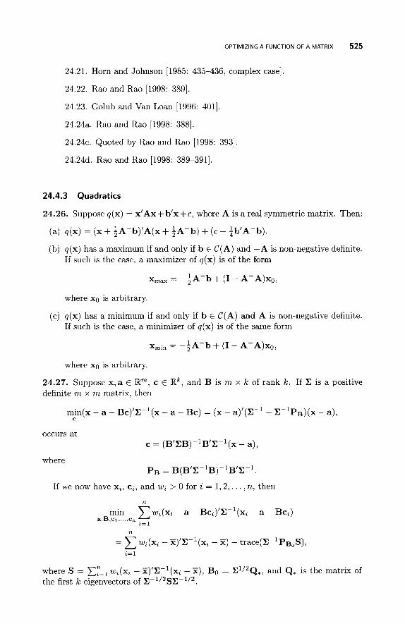
OPTIMIZING A FUNCTION OF A MATRIX 525
24.21. Horn and Johnson [1985: 435-436, complex case].
24.22. Rao and Rao [1998: 3891.
24.23. Golub and Van Loan [1996: 4011.
24.24a. Rao and Rao [1998: 3881.
24.24~. Quoted by Rao and Rao [1998: 3931.
24.24d. Rao and Rao [1998: 389-3911,
24.4.3 Quadratics
24.26. Suppose q(x) = x’Ax + b’x + c, where A is a real symmetric matrix. Then:
(a) q(x) = (x + $A-b)’A(x + iA-b) + (c - ab’A-b).
(b) q(x) has a maximum if and only if b E C(A) and -A is non-negative definite. If such is the case, a maximizer of q(x) is of the form
x,,, = - iA-b + (I - A-A)xo,
where xo is arbitrary.
(c) q(x) has a minimum if and only if b E C(A) and A is non-negative definite. If such is the case, a minimizer of q(x) is of the same form
x,in = -$A-b + (I - A-A)xo,
where xo is arbitrary.
24.27. Suppose x,a E R”, c E Rk, and B is m x k of rank k . If E is a positive definite m x m matrix, then
min(x - a - Bc)’E-’(x - a - Bc) = (x - a)’(E-’ - E - ~ P B ) ( x - a), C
occurs at c = ( B / E B ) - ~ B ~ E - ~ ( ~ - a),
where P B = B(B/E-~B) -~B/E-~ .
If we now have x,, c,, and w, > 0 for z = 1 ,2 , . . . , n, then
n
min C w , ( x , - a - BC,)’E-’(X, - a - BC,) a= 1
a,B,cl , .cn
n
= C w,(x, - %)’E-’(x, - X) - trace(x-lPB,S), 2 1 1
- where S = c:=, w,(x, - x)’E-’(x, - X), Bo = E1/2Q,, and Q* is the matrix of the first k eigenvectors of E-1/2SE-1/2.
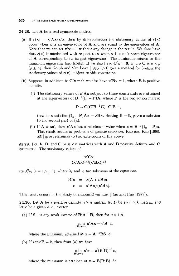
526 OPTIMIZATION AND MATRIX APPROXIMATION
24.28. Let A be a real symmetric matrix.
(a) If T(X) = x’Ax/x’x, then by differentiation the stationary values of T(X)
occur when x is an eigenvector of A and are equal to the eigenvalues of A. Note that we can set x’x = 1 without any change in the result. We then have that T(X) is maximized with respect t o x when x is a unit-norm eigenvector of A corresponding to its largest eigenvalue. The minimum relates to the minimum eigenvalue (see 6.58a). If we also have C’x = 0, where C is n x p ( p 5 n), then Golub and Van Loan [1996: 6211 give a method for finding the stationary values of T(X) subject to this constraint.
(b) Suppose, in addition to C’x = 0, we also have x’Bx = 1, where B is positive definite.
(i) The stationary values of x’Ax subject t o these constraints are attained at the eigenvectors of B-’(I, - P)A, where P is the projection matrix
P = c(c’B-~c)-c’B-~,
that is, x satisfies (I, - P)Ax = XBx. Setting B = I, gives a solution to the second part of (a).
(ii) If A = aa’, then x’Ax has a maximum value when x cx B-’(I, - P)a. This result occurs in problems of genetic selection. Rao and Rao [1998: 5071 give references to two extensions of the above.
24.29. Let A, B, and C be n x n matrices with A and B positive definite and C symmetric. The stationary values of
X’CX (x’ Ax) 1/2 (x’Bx)
(i = 1 ,2 , . . .), where X i and vi are solutions of the equations are
2Cx = X(A+vB)x,
v = x’Ax/(x’Bx)
This result occurs in the study of canonical variates (Rao and Rao [1987])
24.30. Let A be a positive definite n x n matrix, let B be an n x k matrix, and let c be a given Ic x 1 vector.
(a) If S- is any weak inverse of B’A-’B, then for n x 1 x,
min x’Ax = CIS-c,
where the minimum attained at x = A-lBS-c.
B’x=c
(b) If rankB = k , then from (a) we have
min x’x = c’(B’B)-~c, B’x=c
where the minimum is attained at x = B(B’B)-’c.
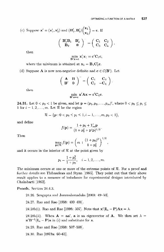
OPTIMIZING A FUNCTION OF A MATRIX 527
Suppose x’ = (xi, x;) and (Bi, B;) (:;) = c . If
then min xix1 = c’Clc,
where the minimum is attained at x1 = B1C;c.
Suppose A is now non-negative definite and c E C(B’). Let
B’x=c
A B ( B ’ O ) - = ( Et -::)’
then min x’Ax = c’C4c
B’x=c
24.31. Let 0 < PO < 1 be given, and let p = (pl,pz,. . . , p m ) ’ , where 0 < po 5 pi 5 1 for z = 1,2, . . . , m. Let R be the region
R = {p : 0 < Po 5 pi 5 1,i = 1,. . . , m , p o < l},
and define
Then
and it occurs in the interior of R at the point given by
The minimum occurs at one or more of the extreme points of R. For a proof and further details see Thibaudeau and Styan [1985]. They point out that their above result applies to a measure of imbalance for experimental designs introduced by Chakabarti [1963].
Proofs. Section 24.4.3.
24.26. Sengupta and Jammalamadaka [2003: 49-50].
24.27. Rao and Rao [1998: 400-4011.
24.28b(i). Rao and Rao [1998: 5071. Note that x’(In - P)Ax = A.
24.28b(ii). When A = aa’, a is an eigenvector of A. We then set X = a’B-’(In - P)a in (i) and substitute for x.
24.29. Rao and Rao [1998: 507-5081.
24.30. Rao [1973a: 60-611.
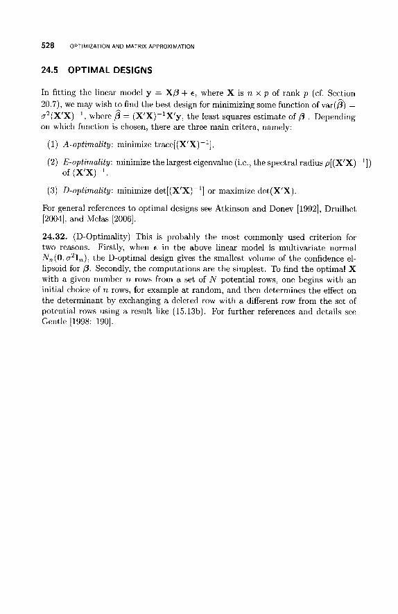
528 OPTIMIZATION AND MATRIX APPROXIMATION
24.5 OPTIMAL DESIGNS
In fitting the linear model y = Xp + E , where X is n x p of rank p (cf. Section 20.7), we may wish to find the best design for minimizing some function of var(B) =
a2(X’X)-l, where ,6 = (X’X)-lX’y, the least squares estimate of p . Depending on which function is chosen, there are three main critera, namely:
(1) A-opt imali ty: minimize trace[(X’X)-l].
(2) E-optimality: minimize the largest eigenvalue (i.e., the spectral radius P[(X’X)-~]) of (X’X)-l.
(3) D-optimality: minimize det[(X’X)-’1 or maximize det(X’X).
For general references to optimal designs see Atkinson and Donev [1992], Druilhet [2004], and Melas [2006].
24.32. (D-Optimality) This is probably the most commonly used criterion for two reasons. Firstly, when E in the above linear model is multivariate normal N,(O, 021n), the D-optimal design gives the smallest volume of the confidence el- lipsoid for p. Secondly, the computations are the simplest. To find the optimal X with a given number n rows from a set of N potential rows, one begins with an initial choice of n rows, for example at random, and then determines the effect on the determinant by exchanging a deleted row with a different row from the set of potential rows using a result like (15.13b). For further references and details see Gentle [1998: 1901.
REFERENCES
Abadir, K. M. and Magnus, J. R. (2005). Matrix Algebra. Cambridge University Press, New York.
Agaian, S. S. (1985). Hadamard Matrices and Their Applications. Springer-.Verlag, New York.
Anderson, T. W. (1955). The integral of a symmetric unimodal function over a symmetric convex set and some probability inequalities. Proceedings of the American Mathemat- ical Society, 6, 170-176.
Anderson, T. W. (1993). Non-normal multivariate distributions: Inference based on el- liptically contoured distributions. In C. R. Rao (Ed.), Multivariate Analysis: Future Directions, Vol. 1, 1-24. North-Holland, Amsterdam.
Anderson, T. W. (1996). Some inequalities for symmetric convex sets with applications. Annals of Statistics, 24, 753-762.
Anderson, T. W. (2003). A n Introduction to Multivariate Statistical Analysis, 3rd ed. John Wiley, New York.
Anderson, T. W. and Styan, G. P. H. (1982). Cochran’s theorem, rank additivity and tripoterit matrices. In G. Kallianpur, P. R. Krishnaiah, and J. K. Ghosh (Eds.), Statis- tics and Probabilzty: Essays in Honor of C. R. Rao, 1-23. North-Holland, New York.
Anderson, W. N. , Jr. and Duffin, R. J . (1969). Series and parallel addition of matrices. SIAM Journal of Applzed Mathematics, 26, 576-594.
Ansley, C. F. (1985). Quick proofs of some regression theorems via the QR algorithm. The American Statistician, 39 ( l ) , 57-59.
Atiqullah, M. (1962). The estimation of residual variance in quadratically balanced least squares problems and the robustness of the F-test. Biometrika, 49, 83-91.
Atkinson, A. C. and Donev, A. N. (1992). Optimum Experimental Designs. Oxford University Press, Oxford, UK.
A Matrix Handbook for Statisticians. By George A. F. Seber Copyright @ 2008 John Wiley & Sons, Inc.
529
530 REFERENCES
Bacharach, M. (1965). Estimating non-negative matrices from marginal data. Interna- tzonal Economic Review, 6, 294-310.
Baksalary, J . K. and Baksalary, 0. M. (2004a). On linear combinations of generalized projectors. Lznear Algebra and Its Applications, 388, 17-24.
Baksalary, J . K. and Baksalary, 0. M. (2004b). Nonsingularity of linear combinations of idempotent matrices. Linear Algebra and Its Applications, 388, 25-29.
Baksalary, J . K. and Baksalary, 0. M. (2004~). Relationships between generalized inverses of a matrix and generalized inverses of its rank-one-modifications. Linear Algebra and Its Applications, 388, 31-44.
Baksalary, J . K. and Puntanen, S. (1990). Spectrum and trace invariance criterion and its statistical applications. Linear Algebra and Its Applications, 142, 121-128.
Baksalary, J. K. and Puntanen, S. (1991). Generalized matrix versions of the Cauchy- Schwarz and Kantorivich inequalities. Aequationes Mathematicae, 41, 103-1 10.
Baksalary, J . K. and Styan, G. P. H. (2002). Generalized inverses of partitioned matrices in Banachiewicz-Schur form. Linear Algebra and Its Applications, 354, 41-47.
Baksalary, J . K., Baksalary, 0. M., and Styan, G. P. H. (2002). Idempotency of linear combinations of an idempotent matrix and a tripotent matrix. Linear Algebra and Its Applications, 354, 21-34.
Baksalary, J. K., Puntanen, S., and Styan, G. P. H. (1990). A property of the disper- sion matrix of the best linear unbiased estimator in the general Gauss-Markov model. Sankhya Series A , 52 (3), 279-296.
Ballantyne, C. S. (1978). Products of idempotent matrices. Linear Algebra and Its Ap- plications, 19, 81-86.
Bapat, R. B. (1990). Permanents in probability and statistics. Linear Algebra and Its Applications. 127, 3-25.
Bapat, R. B. and Raghavan, T. E. S. (1997). Nonnegative Matrices and Applications. Cambridge University Press, Cambridge.
Bartholomew, D. J . (1987). Latent Variable Models and Factor Analysis. Oxford Univer- sity Press, New York.
Basilevsky A. (1983). Applied Matrix Algebra in the Statistical Sciences. North-Holland, Elsevier Science Publishing, New York.
Bates, D. M. (1983). The derivative of the determinant of X'X and its uses. Technomet- rics, 25, 373-376.
Bates, D. M. and Watts, D. G. (1985). Multiresponse estimation with special application to linear systems of differential equations (with Discussion). Technometrics, 27, 329- 360.
Bates, D. M. and Watts, D. G. (1987). A generalized Gauss-Newton procedure for mul- tiresponse parameter estimation. SIAM Journal of Science and Statistical Computing, 8, 49-55.
Bates, D. M. and Watts, D. G. (1988). Nonlinear Regression Analysis. John Wiley, New York.
Bellman, R. (1970). Introduction to Marix Analysis, 2nd ed. McGraw-Hill, New York.
BCnasskni, J. (2002). A complementary proof of an eigenvalue property in correspondence analysis. Linear Algebra and Its Applications, 354, 49-51.
Ben-Israel, A. and Greville, T. N. E. (2003). Generalized Inverses: Theory and Applica- tions, 2nd ed. Springer-Verlag, New York.
Berkovitz, L. D. (2002). Convexity and Optimization in R". John Wiley, New York.
Berman, A. and Plemmons, R. J. (1994). Non-negative Matrices in the Mathematical Sciences. SIAM, Philadelphia. Originally published in 1979 by Academic Press.
REFERENCES 531
Berman, A. and Shaked-Monderer, N. (2003). Completely Positive Matrices. World Sci-
Bhatia, R. (1997). Matrix Analysis. Springer, New York.
Bhaumik, D. K. (1995). Majorization and D-optimality for complete block designs under
Bini, D., Tyrtyshnikov, E., and Yalamov, P. (2001). Structured Matrices: Recent Devel-
Birkhoff, G. and Varga, R. S. (1958). Reactor criticality and non-negative matrices.
Bloomfield, P. and Watson, G. S. (1975). The inefficiency of least squares. Biometrika,
Boshnakov, G. N. (2002). Multi-companion matrices. Linear Algebra and Its Applications,
Bottcher, A. and Silbermann, B. (1999). Introduction to Large Truncated Toeplitz Matri- ces. Springer, New York.
Boullion, T . L. and Odell, P. L. (1971). Generalized Inverse Matrices. John Wiley, New York.
Brillinger, D. R. (1975). Times Series : Data Analysis and Theory. Holt, Rinehart and Winston, New York.
Brown, P. J . (2002). Inverted Wishart distribution, generalized. In A. H. El-Shaarwi and W. W. Piegorsch (Eds), Encyclopedia of Environmetrics. John Wiley, New York
Bullen, P. S. (2003). Handbook of Means and Their Inequalities. Kluwer, Netherlands. Calvert, B. and Seber, G. A. F. (1978). Minimisation of functions of a positive semidefinite
Campbell, S. L. and Meyer, C. D. (1979). Generalized Inverses of Linear Transformations.
Carlitz, L. (1959). Some cyclotomic matrices. Acta Arithmetica 5 , 293-308. Carmeli, M. (1983). Statistical Theory and Random Matrices. Marcel Dekker, New York. Carroll, R. J. and Ruppert, D. (1988). Transformation and Weighting in Regression.
Chapman and Hall, London.
Carroll, R. J., Ruppert, D., and Stefanski, L. A. (2006), Measurement Error in Nonlinear Models: A Modern Perspective, 2nd ed. Chapman and Hall/CRC, Boca Raton, FL.
Caswell, H. (2001). Matrix Population Models, 2nd ed. Sinauer Associates, Sunderland, MA.
Caswell, H. (2006). Applications of Markov chains in demography. In A. N. Langville and W. J. Stewart (Eds), MAM2006: Markov Anniversary Meeting, 319-334. Boson Books, Raleigh, NC.
10, in press.
Indian Statistical Association, 1, 8-23.
New York.
entific, Hackensack, NJ.
correlations. Journal of the Royal Statistical Society, Series B , 57, 139-143.
opments in Theory and Computation. Nova Science Publishers, Inc., New York.
Journal of the Society for Industrial and Applied Mathematics, 6, 354-377.
62, 121-128.
354, 53-83.
matrix A subject to A X = 0. Journal of Multivariate Analysis, 8 , 274-281.
Pitman, London.
Caswell, H. (2007). Sensitivity analysis of transient population dynamics. Ecology Letters,
Chakrabarti, M. C. (1963). On the C-matrix in design of experiments. Journal of the
Ching, W.-K. (2006). Markov Chains: Models, Algorithms and Applications. Springer,
Christensen, R. (1997). Log-linear Models and Logistic Regression. Springer, New York.
Christensen, R. (2001). Advanced Linear Modeling: Multivariate, Times Series, and Spatial Data; Nonparametric Regression and Response Surface Maximization, 2nd ed. Springer, New York.
Christensen, R. (2002). Plane Answers to Complex Questions: The Theory of Linear Models, 3rd ed. Springer, New York.
532 REFERENCES
Chu, K. L., Isotalo, J., Puntanen, S., and Styan, G. P. H. (2004). On decomposing the Watson efficiency of ordinary least squares in a partitioned weakly singular model. Sunkha: The Indian Jounal of Statistics, 66 (4), 634-651.
Chu, K. L., Isotalo, J., Puntanen, S., and Styan, G. P. H. (2005a). Some further results concerning the decomposition of the Watson efficiency in partitioned linear models. Sankha: The Indian Jounal of Statistics, 67 ( l ) , 74-89.
Chu, K. L., Isotalo, J., Puntanen, S., and Styan, G. P. H. (2005b). The efficiency factoriza- tion multiplier for the Watson efficiency in partitioned linear models; Some examples and a literature review. Research Letters in the Information and Mathematical Sci- ences, 8, 165-187. Available online at http://iims.massey.ac.nz/research/letters/.
Clarke, M. R. B. (1971). Algorithm AS41: Updating the sample mean and dispersion matrix. Applied Statistics, 20, 206-209.
Cox, D. R. and Hinkley, D. V. (1974). Theoretical Statistics. Chapman and Hall, London.
Cullen, C. G. (1997). Linear Algebra with Applications, 2nd ed. Addison-Wesley, Reading, MA.
Dagum, E. B. and Luati, A. (2004). A linear transformation and its properties with special application in times series filtering. Linear Algebra and Its Applications, 388, 107-1 17.
Darroch, J. N. and Silvey, S. D. (1963). On testing more than one hypothesis. Annals of Mathematical Statistics, 34, 555-567.
Davis, P. J. (1979). Circulant Matrices. John Wiley, New York.
Debreu, G. and Herstein, I. N. (1953). Nonnegative square matrices. Econornetrica, 21,
Deemer, W. L. and Olkin, I. (1951). The Jacobians of certain matrix transformations useful in multivariate analysis. Biometrika, 38, 345-367.
Dernetrius, L. (1971). Primitivity conditions for growth matrices. Mathematical Bio- sciences, 12, 53-58.
Dobson, A. J . (2001). A n Introduction to Generalized Linear Models, 2nd ed. Chapman and Hall, London.
Dhrymes, P. J . (2000). Mathematics for Econometrics, 3rd ed. Springer-Verlag, New York.
Dragomir, S. S. (2004). Discrete Inequalities of the Cauchy-Bunyakowsky-Schwarz Type. Nova Science Publishers, New York.
Dress, A. W. M. and Wenzel, W. (1995). A simple proof of an identity concerning pfaffians of skew symmetric matrices. Advances in Mathematics, 112, 120-134.
Driscoll, M. F. and Krasnicka, B. (1995). An accessible proof of Craig’s theorem in the general case. The American Statistician, 49 ( l ) , 59-62.
Druilhet, P. (2004). Conditions for optimality in experimental designs. Linear Algebra and Its Applzcations, 388, 147-157.
Drury, S. W., Liu, S., Lu, C.-Y., Puntanen, S., and Styan, G. P. H. (2002). Some comments on several matrix inequalities with applications t o canonical correlations; historical background and recent developments. Sankhii A , 62, 453-507.
Drygas, H. (1970). The Coordinate Free Approach to Gauss-Markov Estimation. Lecture Notes in Operations Research and Mathematical Systems, 40. Springer-Verlag, Berlin.
Duff, I. S., Erisman, A. M., and Reid, J . K . (1986). Direct Methods for Sparse Matrices. Clarendon Press, Oxford.
Dumbgen, L. (1995). A simple proof and refinement of Wielandt’s eigenvalues inequality. Statistics & Probability Letters, 25, 113-115.
Dwyer, P. S. (1967). Some applications of matrix derivatives in multivariate analysis. Journal of the American Statistical Association, 62, 607-625.
597-607.
REFERENCES 533
Eaton, M. L. and Perlman, M. D. (1973). The non-singularity of generalized sample covariance matrices. Annals of Statistics, 1, 710-717.
Eaton, M. L. and Tyler, D. E. (1991). On Wielandt’s inequality and its application to the asymptotic distribution of the eigenvalues of a random symmetric matrix. Annals of Statistics, 19, 260-271.
Edelman, A. (1997). The probability that a random real Gaussian matrix has k real eigenvalues, related distributions and the circular law. Journal of Multivariate Analysis, 60, 203-232.
Elsner, L. (1982)). On the variation of the spectra of matrices. Linear Algebra and Its Applications, 7, 127-138.
Esary, J. D., Proschan, F., and Walkup, D. W. (1967). Associated random variables, with applications. The Annals of Mathematical Statistics, 38, 1466-1474.
Escobar, L. A. and Moser, E. B. (1993). A note on the updating of regression estimates. The American Statistician, 47, 192-194.
Eubank, R. L. and Webster, J . T. (1985). The singular-value decomposition as a tool for solving estimability problems. The American Statistician, 39 (I), 64-66.
Everitt, B. S. (1984). A n Introduction to Latent Variable Models. Chapman and Hall, London.
Everitt, B. S. (1993). Cluster Analysis, 3rd ed. Hodder and Stoughton, London. Fan, K. (1949). On a theorem of Weyl concerning eigenvalues of linear transformations I.
Proceedings of the National Academy of Sciences of the USA, 35, 652-655. Fan, K. (1951). Maximum properties and inequalities for eigenvalues of completely con-
tinuous operators. Proceedings of the National Academy of Sciences of the USA, 37,
Fang, K.-T. and Anderson, T. W. (Eds.) (1990). Statistical Inference in Elliptically Contoured and Related Distributions. Allerton Press, New York.
Fang, K.-T., Kotz, S., and Ng, K.-W. (1990). Symmetric Multivariate and Related Dis- tributions. Chapman and Hall, New York.
Faraway, J . J. (2006). Extending the Linear Model with R: Generalized Linear, Mixed Effects and Nonparametric Models. Chapman and Hall/CRC, FA, USA.
Farebrother, W. (1976). Further results on the mean square error of ridge regression. Journal of the Royal Statistical Society B, 38, 248-250.
Farnum, N. R. (1989). An alternative proof of Samuelson’s inequality and its extensions. The American Statistician, 43 ( l ) , 46-47.
Flury, B. (1988). Common Principal Components and Related Multivariate models. John Wiley, New York.
Friedberg, S. H., Insel, A. J., and Spence, L. E. (2003). Linear Algebra, 3rd ed. Pearson Education, Upper Saddle River, NJ.
Galambos, J . and Simonelli, I. (1996). Bonferroni-type Inequalities with Applications. Springer-Verlag, New York.
Gantmacher, F. R. (1959). The Theory of Matrices, Vol. 1. Chelsea Publishing Co., New York.
Gentle, J. E. (1998). Numerical Linear Algebra for Applications in Statistics. Springer, New York.
Girko, V. L. and Gupta, A. K., (1996). Multivariate elliptically contoured linear models and some aspects of the theory of random matrices. In A. K. Gupta and V. C. Girko (Eds.), Proceedings of the Sixth Lukacs Symposium, Analysis and Theory of Random Matrices, 327-386. VSL, The Netherlands.
Golub, G. H and Van Loan, C. F. (1996). Matrix Computations, 3rd ed. John Hopkins University Press, Baltimore.
760-766.
534 REFERENCES
Golyandina, N., Nekrutkin, V., and Zhigljavsky, A. (2001). Analysis of Time Series Struc- ture: SSA and Related Techniques. Monographs on Statistics and Applied Probability, 90. Chapman and Hall/CRC, Boca Raton, FL.
Goodman, N. R. (1963). Statistical analysis based upon a certain multivariate complex Gaussian distribution (an introduction). Annals of Mathematical Statistics, 34, 152- 177.
Gordon, A. D. (1999). Classification, 2nd ed. Chapman and Hall, Boca Raton, FL. Gower, J. C. and Dijksterhuis, G. B. (2004). Procrustes Problems. Oxford Statistical
Science Series 30, Oxford University Press.
Graham, A. (1981). Kronecker Products and Matrix Calculus. Ellis Horwood, Chichester, UK.
Graham, A. (1987). Nonnegative Matrices and Applicable Topics in Linear Algebra. Ellis Horwood, Chichester, UK.
Graybill, F. A. (1983). Matrices With Applications in Statistics, 2nd ed. Wadsworth, Belmont, CA.
Greenbaum, A. (2007). Iterative solution methods for linear systems. In L. Hogben (Ed.), Handbook of Linear Algebra, Chapter 41. Chapman and Hall/CRC, Taylor and Francis Group, Boca Raton, FL.
Greenberg, B. G. and Sarhan, A. E. (1959). Matrix inversion, its interest and application in data analysis. Journal of the American Statistical Association, 54, 755-766.
Grenander, U. and Szego, G. (1958). Toeplitz Forms and their Applications. University of California Press, Berkeley, CA.
Greub, W. and Rheinboldt, W. (1959). On a generalization of an inequality of L. V. Kantorovich. Proceedings of the American Mathematical Society, 10, 407-415.
Gro6, J. (1999). Solution to a rank equation. Linear Algebra and Its Applications, 289,
Groi3, J. (2000). The Moore-Penrose inverse of a partitioned nonnegative definite matrix. Linear Algebra and Its applications, 321, 113-121.
Gro6, J. (2003). Linear Regression. Springer, New York.
Gro6, J. (2004). The general Gauss-Markov model with possibly singular covariance
Groves, T. and Rothenberg, T. (1969). A note on the expected value of an inverse matrix.
Gupta, A. K. and Varga, R. (1993). Elliptically Contoured Models in Statistics. Kluwer
Gustafson, K. E. (1968). The angle of an operator and positive operator products. Bulletin
Gustafson, K. E. (2000). An extended operator trigonometry. Linear Algebra and Its
Gustafson, K. E. (2002). Operator trigonometry of statistics and economics. Linear
Gustafson, K. E. (2005). The geometry of statistical efficiency. Research Letters in the
127-1 30.
matrix. Statistical Papers, 45, 311-336.
Biometrika, 56, 690-691.
Academic, Dordrecht.
of the American Mathematical Society, 74, 488-492.
Applications, 319, 117-135.
Algebra and its Applications, 354, 141-158.
Information and Mathematical Sciences, 8, 105-121. Available online a t http://iims.massey.ac.nz/research/letters/.
Gustafson, K. E. and Rao, D. K. M. (1997). Numerical Range: The Field of Values of Linear Operators and Matrices. Springer, New York.
Guttman, L. (1955). A generalized simplex for factor analysis. Psychometrika, 20, 173- 192.
Hager, W. W. (1989). Updating the inverse of a matrix. SIAM REview, 11 (2), 221-239.
REFERENCES 535
Halmos, P. R. (1958). Finite-Dimensional Vector Spaces. Van Nostrand, New York. Halton, J . H. (1966a). A combinatorial proof of Cayley’s theorem on Pfaffians. Journal
of Combinatorial Theory, 1, 224-232. Halton, J . H. (1966b). An identity of the Jacobi type for Pfaffians. Journal of Combina-
torial Theory, 1, 333-337. Hanson, A. T. (2006). Visualizing Quaternions. Elsevier, Morgan Kaufmann Publishers,
San Francisco, CA. Hardy, G. H., Littlewood, J. E., and Pdya , G. (1952). Inequalities. Cambridge University
Press, Cambridge, UK. Harville, D. A. (1997). Matrix Algebra f rom a Statistician’s Perspective. Springer, New
York. Harville, D. A. (2001). Matrix Algebra: Exercises and Solutions. Springer-Verlag, New
York. Henderson H. V. and Searle, S. R. (1979). Vec and vech operators for matrices, with some
uses in Jacobians and multivariate statistics. Canadian Journal of Statistics, 7, 65-81. Henderson H. V. and Searle, S. R. (1981a). The vec-permutation matrix, the vec operator
and Kronecker products. Linear and Multilinear Algebra, 9, 271-288. Henderson H. V. and Searle, S. R. (1981b). On deriving the inverse of a sum of matrices.
SIAM Review, 23, 53-60. Henderson H. V., Pukelsheim, F., and Searle, S. R. (1983). On the history of the Kno-
necker product. Linear and Multilinear Algebra, 14, 113-120. Hernindez-Lerma, 0. and Lasserre, J. B. (2003). Markov Chains and Invariant Probabil-
ities. Birkhauser, Boston. Hochberg, Y. and Tamhane, A. C. (1987). Multiple Comparison Procedures. John Wiley,
New York. Hoeffding, W. (1963). Probability inequalities for sums of bounded random variables.
Journal of the American Statistical Association, 58, 13-30. Hoppensteadt, F., Salehi, H., and Skorokhod, A. (1996). On the asymptotic behaviour of
Markov chains with small random perturbations of transition probabilities. In A. K. Gupta and V. C. Girko (Eds.), Proceedings of the Sixth Lukacs Symposium, Analysis and Theory of Random Matrices, 93-100. VSL, The Netherlands.
Horn R. and Johnson, C.A. (1985). Matrix Analysis. Cambridge University Press, Cam- bridge, UK. Corrected reprint edition (1990), which I was unaware of in time to incor- porate any changes there may have been in the theorem statements.
Horn R. and Johnson, C.A. (1991). Topics in Matrix Analysis. Cambridge University Press, Cambridge, UK.
Hotelling, H. (1933). Analysis of a complex of statistical variables into principal compo- nents. Journal of Educational Psychology, 24, 417-441.
Hsu, J . C. (1996). Multiple Comparisons: Theory and Methods. Chapman and Hall, London.
Hsu, P. L. (1953). On symmetric, orthogonal and skew-symmetric matrices. Proceedings of the Royal Society of Edinburgh, 10, 37-44.
Hunter, C. M. and Caswell, H. (2005). The use of the vec-permutation matrix in spatial matrix population models. Ecological Modelling, 188, 15-21.
Hunter, J . J. (1983a). Mathematical Techniques of Applied Probability, Vol. 1. Academic Press, New York.
Hunter, J . J . (1983b). Mathematical Techniques of Applied Probability, Vol. 2. Academic Press, New York.
Hunter, J . J. (1988). Characterizations of generalized inverses associated with Markovian kernels. Linear Algebra and Its Applications, 102, 121-142.
536 REFERENCES
Hunter, J . J . (1990). Parametric forms for generalized inverses of Markovian kernels and
Hunter, J . J. (1991). The computation of stationary distributions of Markov chains Journal of Applied Mathematics and Stochastic Analysis, 4
Hunter, J . J . (1992). Stationary distributions and mean first passage times in Markov Asia-Pacific Journal of Operational Research, 9,
Hunter, J . J . (2005). Stationary distributions and mean first passage times of perturbed Markov chains. Linear Algebra and Its Applications, 410, 217-243.
Isotalo, J., Puntanen, S., and Styan, G. P. H. (2005a). Formulas Useful for Linear Regres- sion Analysis and Related Matrix Theory, 3rd ed. Report A 350, Dept. of Mathematics, Statistics, and Philosophy, University of Tampere, Tampere, Finland, 85 pp.
Isotalo, J . , Puntanen, S., and Styan, G. P. H. (2005b). Matrix Tricks for Linear Statistical Models: Our Personal Top Sixteen, 3rd ed. Report A 363, Dept. of Mathematics, Statistics, and Philosophy, University of Tampere, Tampere, Finland, 207 pp.
Jeffrey, D. J . and Corless, R. M. (2007). Linear algebra in Maple. In L. Hogben (Ed.), Handbook of Linear Algebra, Chapter 72. Chapman and Hall/CRC, Taylor and Francis Group, Boca Raton, FA.
Jewell, N. P. and Bloomfield, P. (1983). Canonical correlations of past and future for times series. Annals of Statistics, 11, 837-847.
John, J. A. (2001). Updating formula in an analysis of variance model. Biometrika, 88,
John, J . A. and Williams, E. R. (1995). Cyclic and Computer Generated Designs, 2nd ed. Monographs on Statistics and Applied probability, 38. Chapman and Hall, London, UK.
their applications. Linear Algebra and Its Applications, 127, 71-84.
through perturbations. ( l) , 29-46.
chains using generalised inverses. 145-153.
1175-1 178.
Jolliffe, I. T. (2002). Principal Component Analysis, 2nd ed. Springer, New York. Kabe, D. G. (1980). On extensions of Samuelson’s inequality (Letter to the Editor). The
Kantor, I. L. and Solodovnikov, A. S. (1989). Hypercomplex Numbers: A n Elementary
Kariya, T. and Kurata, H. (2004). Generalized Least Squares. Wiley, New York. Kariya, T. and Sinha, B. K. (1989). Robustness of Statistical Tests. Academic Press,
Kaufman, L. and Rousseuw, P. J. (1990). Finding Groups in Data: A n Introduction to
Kelly, P. J . and Weiss, M. L. (1979). Geometry and Convexity. John Wiley, New York. Kempthorne, 0. (1980). The term design matrix. The American Statistician, 34 (4), 249. Khatri, C. G. and Rao, C. R. (1981). Some extensions of the Kantorovich inequality and
statistical applications. Journal of Multivariate Analysis, 11, 498-505. Khatri, C. G. and Rao, C. R. (1982). Some generalizations of the Kantorovich inequality.
Sankhy6 A , 44, 91-102. Khattree, R. (1996). Multivariate statistical inferences involving circulant matrices. In A.
K. Gupta and V. C. Girko (Eds.), Proceedings of the Sixth Lukacs Symposium, Analysis and Theory of Random Matrices, 101-110. VSL, The Netherlands.
Klein, T. (2004). Invariant symmetric block matrices for the design of mixture experi- ments. Linear Algebra and Its Applications, 388, 261-278.
Knott, M. (1975). On the minimum efficiency of least squares. Biometrika, 62, 129-132. Koliha, J . J., RakoEeviC, V., and StraSkraba, I. (2004). The difference and sum of projec-
American Statistician, 34 (4), 249.
Introduction to Algebras. Springer-Verlag, Berlin.
Boston.
Cluster Analysis. John Wiley, New York.
tors. Linear Algebra and Its Applications, 388, 279-288.
REFERENCES 537
Kollo, T. and Neudecker, H. (1993). Asymptotics of eigenvalues and unit-length eigen- vectors of sample variance and correlation matrices. Journal of Multivariate Analysis, 47, 283-300. Corrigendum: 1994, 51, 210.
Kollo, T. and Neudecker, H. (1997). Asymptotics of Pearson-Hotelling principal-component vectors of sample variance and correlation matrices. Behaviometrika, 24 (1), 51-69.
Kollo, T. and von Rosen, D. (2005). Advanced Multivariate Statistics with Matrices. Springer, New York.
Kotz, S. and Nadarajah, S. (2004). Multivariate t Distributions and Their Applications. Cambridge University Press, New York.
Kounias, E. (1968). Bounds for the probability of a union of events, with applications. Annals of Statistics, 39, 2154-2158.
Krishnaiah, P. R. (1976). Some recent developments on complex multivariate distribution. Journal of Multivariate Analysis, 6, 1-30.
Krzanowski, W. J . (1988). Principles of Multivariate Analysis. Clarendon Press, Oxford, UK.
Lancaster, P. (1964). On eigenvalues of matrices dependent on a parameter. Numerische Mathematik, 6, 337-346.
Latour, D., Puntanen, S., and Styan, G. P. H. (1987). Equalities and inequalities for the canonical correlations associated with some partitioned generalized inverses of a covariance matrix. Proceedings of the Second International Tampere Seminar on Linear Statistical Models and Their Applications, 541-553. Dept. of Mathematical Sciences, University of Tampere, Finland.
Lay, D. C. (2003). Linear Algebra and Its Applications, 3rd ed. Addison Wesley, Boston. Lay, S. R. (1982). Convex Sets and Their Applications. John Wiley, New York. Lee, A. J . , Nyangoma, S. O., and Seber, G. A. F. (2002). Confidence regions for multino-
mial parameters. Computational Statistics & Data Analysis, 39, 329-342. Leon, S. J . (2007). Matlab. In L. Hogben (Ed.), Handbook of Linear Algebra, Chapter 71.
Chapman and Hall/CRC, Taylor and Francis Group, Boca Raton, FL.
Lidskii, V. (1950). The proper values of the sum and product of symmetric matrices. Dokl. Akad. Nauk. SSSR, 75, 769-772 (in Russian). (Translated by C. D. Benster, U.S. Department of Commerce, National Bureau of Standards, Washingon, D.C., N.B.S. Rep. 2248, 1953).
A further note on a theorem on the difference of the generalized inverses of two non-negative definite matrices. Communications in Statistics-Theory and Methods, 18 (5), 1747-1751.
Liu, S. (2002a). Several inequalities involving Khatri-Rao products of positive semidefinite matrices. Linear Algebra and Its Applications, 354, 175-186.
Liu, S. (2002b). Local influence in multivariate elliptical linear regression models. Linear Algebra and Its Applications, 354, 159-174.
Liu, S. and Neudecker, H. (1996). Several matrix Kantorovich-type inequalities. Journal of Mathematical Analysis and Applications, 197, 23-26.
McCullagh, P. and Nelder, J. A. (1989). Generalized Linear Models, 2nd ed. Chapman and Hall, New York.
McLachlan, G. J . (1992). Discriminant Analysis and Statistical Pattern Recognition. John Wiley, New York. Reproduced in paperback, Wiley-Interscience Series (2004), Hobo- ken, NJ.
MacRae, E. C. (1974). Matrix derivatives with an application to an adaptive decision problem. Annals of Statistics, 2 ( 2 ) , 337-346.
Magnus, J. R. (1978). The moments of products of quadratic forms in normal variables. Statistica Neerlandica, 32, 201-210.
Liski, E. P. and Puntanen, S. (1989).
538 REFERENCES
Magnus, J . R. (1982). Multivariate error components analysis of linear and nonlinear regression models by maximum likelihood. Journal of Econometrics, 19, 239-285.
Magnus, J . R. (1988). Linear Structures. Charles Griffin, London and Oxford University Press, New York.
Magnus, J . R. and Neudecker, H. (1979). The commutation matrix: Some properties and applications. Annals of Statistics, 7, 381-394.
Magnus, J . R. and Neudecker, H. (1999). Matrix Differential Calculus: With Applications in Statistics and Econometrics, revised ed. John Wiley, Chichester, UK.
Maindonald, J . H. (1984). Statistical Computation. John Wiley, New York. Makelainen, T. (1970). Extrema for characterisic roots of product matrices. Soc. Sci.
Fenn. Commentationes Physico-Mathematicae, 38 (4), 27-53. Makelainen, T., Schmidt, K., and Styan, G. P. H. (1981). On the existence and uniqueness
of the maximum likelihood estimate of a vector-valued parameter in fixed-size samples. Annals of Statistics, 9, 758-767.
Mandel, J . (1982). Use of the singular value decomposition in regression analysis. The Amencan Statistician, 36 ( l ) , 15-24.
Marcus, M. and Minc, H. (1964). A Suntey of Matrix theory and Matrix Inequalities. Allyn and Bacon, Boston.
Marsaglia, G. and Styan, G. P. H. (1974a). Equalities and inequalities for ranks of matri- ces. Linear and Multilinear Algebra, 2 , 269-292.
Marsaglia, G. and Styan, G. P. H. (1974b). Rank conditions for generalized inverses of partitioned matrices. Sankhya, 36, 437-442.
Marshall, A. W. and Olkin, I. (1979). Inequalities; Theory of Majorization and Its Appli- cations. Mathematics in Science and Engineering, 143. Academic Press, New York.
Marshall, A. W. and Olkin, I. (1990). Matrix versions of the Cauchy and Kantorovich inequalities. Aequationes Mathematicae, 40, 89-93.
Mathai, A. M. (1997). Jacobians of Matrix Transformations and Functions of Matrix Argument. World Scientific, Singapore.
Mathai, A. M. and Provost, S. B. (1992). Quadratic Forms in Random Variables: Theory and Applications. Marcel Dekker, New York.
Mathai, A. M. and Provost, S. B. (2005). Some complex matrix-variate statistical distri- butions on rectangular matrices. Linear Algebra and Its Applications, 410, 198-216.
Mehta, M. L. (1989). Matrix Theory. Les Editions de Physique, 91944 Les Ulis Cedex, France.
Mehta, M. L. (2004). Random Matrices, 3rd ed. Elsevier Academic Press, New York. Meijer, E. (2005). Matrix algebra for higher order moments.
Melas, V. B. (2006). Functional Approach to Optimal Design. Springer, New York. Merikoski, J. K. and Virtanen, A. (2004). The best possible lower bound for the Perron
root using traces. Linear Algebra and Its Applications, 388, 301-313. Meyer, C. D. (1975). The role of the group generalized inverse in the theory of finite
Markov chains. SIAM Review, 17 (3), 443-464. Meyer, C. D. (2000). Matrix Analysis and Applied Linear Algebra. SIAM, Philadelphia.
See www.matrixanalysis.com/Errata.html for a list of errata (which do not affect my book).
Miller, R. G. (1981). Simultaneous Statistical Inference, 2nd edit. McGraw-Hill, New York.
Minc, H. (1978). Permanents. Addison-Wesley, Reading, MA. Minc, H. (1987). Theory of Permanents 1982-1985. Lznear and Multilinear Algebra, 21,
Linear Algebra and Its Applications, 410, 112-134.
109-148.
REFERENCES 539
Mitra, S. K. and Puntanen, S. (1991). The shorted operator and generalized inverses of matrices. Calcutta Statistical Association Bulletin, 40, 97-102.
Mitra, S. K., Puntanen, S., and Styan, G. P. H. (1995). Shorted matrices and their applications in linear statistical models: A review. Multivariate Statistics and Matrices in Statistics: Proceedings of the 5th Tartu Conference, Tartu-Piihajarve, Estonia, 23-28 May 1994. In E.-M. Tiit, T. Kollo, and H. Niemi (Eds.), New Trends in Probability and Statzstics, Vol. 3, 289-311. VSP, Utrecht, Netherlands, and TEV, Vilnius, Lithuania.
Mitra, S. K. and Puri, M. L. (1979). Shorted operators and generalized inverses of matri- ces. Linear Algebra and Its Applications, 25, 45-56.
Moore, E. H (1935). General analysis. Memoirs of the American Philosophical Society, 1,
Mudholkar, G. S. (1965). A class of tests with monotone power functions for two problems in multivariate statistical analysis. Annals of Mathematzcal Statistics, 36, 1794-1801.
Mudholkar, G. S. (1966). On confidence bounds associated with multivariate analysis and non-independence between two sets of variates. Annals of Mathematical Statistics, 37,
Muirhead, R. J. (1982) Aspects of Multivariate Statistical Theory. John Wiley, New York. Mulholland, H. P. and Smith, C. A. B. (1959). An inequality arising in genetical theory.
Nel, D. G. (1980). On matrix differentiation in statistics. South African Statistical Jour-
Nelder J. A. (1985). An alternative interpretation of the singular-value decomposition in
Neudecker, H. (2003). On two matrix derivatives by Kollo and von Rosen. SORT, 27 (a),
Neudecker, H. and Liu, S. (1994). Letters to the editor. The American Statistician, 48 (4), 351.
Neudecker, H. and Trenkler, G (2002). Third and fourth moment matrices of vecX’ in multivariate analysis. Linear Algebra and Its Applications, 354, 223-229.
Norris, J. R. (1997). Markov Chains. Cambridge University Press, New York.
Northcott, D. G. (1984). Multilinear Algebra. Cambridge University Press, Cambridge.
Noumann, M. and Xu, J . (2005). A parallel algorithm for computing the group inverse via Perron complementation. Electronic Journal of Linear Algebra, 13, 131-145.
Okamoto, M. (1973). Distinctness of the eigenvalues of a quadratic form in a multivariate sample. Annals of Statistics, 1, 763-765.
Okamoto, M. and Kanazawa, M. (1968). Minimization of eigenvalues of a matrix and optimality of principal components. Annals of Mathematical Statistics, 39, 859-863.
Olkin, I. (1953). Note on the Jacobians of certain matrix transformations useful in mul- tivariate analysis. Biometrika, 40, 43-46.
Olkin, I. (2002). The 70th anniversary of the distribution of random matrices. Linear Algebra and Its Applications, 354, 231-243.
Olkin, I. and Sampson, A. R. (1972). Jacobians of matrix transformations and induced functional equations. Linear Algebra and Its Applications, 5 , 257-276.
Ostrowski, A. M. (1973). Solutions of Equations in Euclidean and Banach Spaces. Aca- demic Press, New York.
Ouellette, D. V. (1981). Schur complements and statistics. Linear Algebra and Its Appli- cations, 36, 187-195.
Pan, J.-X. and Fang, K.-T. (2002). Growth Curve Models and Statistical Diagnostics. Springer, New York.
147-209.
1736-1746.
American Mathematical Monthly, 66, 673-683.
nal, 14, 137-193.
regression. The American Statistician, 39 ( l ) , 63-64.
153-164.
540 REFERENCES
Parameswaran, S. (1954). Skew-symmetric determinants. The American Mathematical Monthly, 61 (2), 116.
Parthsarathy, T. and Raghaven, T. E. S. (1971). Some Topics in Two Person Games. Elsevier, New York.
Penrose, R. A. (1955). A generalised inverse for matrices. Proceedings of the Cambridge Philosophical Society, 51, 406-413.
Penrose, R. (1956). On best approximate solutions of linear matrix equations. Proceedings of the Cambridge Philosophical Society, 52, 17-19.
Perlman, M. D. (1990). T.W. Anderson’s theorem on the integral of a symmetric function over a symmetric convex set and its applications in probability and statistics. In G. P. H. Styan (Ed.), The Collected Papers of T. W. Anderson, 1943-1985, 2, 1627-1641. John Wiley, New York.
Perlman, M. D. (1993). Concentration inequalities for multivariate distributions: 11. El- liptically contoured distributions. In M. Shaked and Y. L. Tong (Eds.), Stochastic Inequalities, IMS Lecture Notes-Monograph Series, 22, 284-308. Institute of Mathe- matical Statistics, Hayward, Californina.
Potthoff,, R. F. and Roy, S. N. (1964). A generalized multivariate analysis of variance model useful especially for growth curve models. Biometrika, 51, 313-326.
Pronzato, L, Wynn, H. P., and Zhigljavsky, A. (2005). Kantorovich-type inequalities for operators via D-optimal design theory. Linear Algebra and Its Applications, 410,
Puntanen, S. and Styan, G. P. H. (1989). The equality of the ordinary least squares estimator and the best linear unbiased estimator (with comments by Oscar Kempthorne and by Shayle Searle, and with “Reply” by the authors). The American Statistician, 43 (3), 153-164. See also further comments in 44 (2), 191-192.
Puntanen, S. and Styan, G. P. H. (2005a). Historical introduction: Issai Schur and the early development of the Schur complement. In F. Zhang (Ed.), The Schur Complement and Its Applications, 1-16, Springer, New York.
Puntanen, S. and Styan, G. P. H. (2005b). Schur complements in statistics and probability. In F. Zhang (Ed.), The Schur Complement and Its Applications, 163-226. Springer, New York.
Puntanen, S. and Styan, G. P. H. (2006). Chapter 52: Random Vectors and Linear Statistical Models. In L. Hogben (Ed.), Handbook of Linear Algebra, 52.1-52.17. Taylor and Francis Group, Boca Raton, FL.
Puntanen, S., Styan, G. P. H., and Jensen, S. T. (1998). Three Biblographies and a Guide: A third Guide on Books on Matrices and Books on Inequalities with Statistical and Other Applications, The Seventh Inernational Workshop on Matrices and Statistics, in Celebration of T. W. Anderson’s 80th Birthday, Fort Lauderdale, Florida, 27-100. Nova Southern University, Fort Lauderdale, FL.
Puntanen, S., Styan, G. P. H., and Werner, H. J. (2000). Two matrix-based proofs that the linear estimator Gy is the best linear unbiased estimator. Journal of Statistical Planning and Inference, 88, 173-179.
Rao, A. R. and Bhimasankaram, P. (2000). Linear Algebra, 2nd ed. Hindustan Book Agency, New Delhi.
Rao, C. R. (1973a). Linear Statistical Inference and Its Applications, 2nd ed. John Wiley, New York.
Rao, C. R. (1973b). Representations of best linear unbiased estimators in the Gauss- Markoff model with a singular dispersion matrix. Journal of Multivariate Analysis, 3,
160-169.
276-292.
REFERENCES 541
Rao, C. R. (1978). Choice of best linear estimators in the Gauss-Markoff model with a singular dispersion matrix. Communications in Statistics-Theory and Methods, 7,
Rao, C. R. (1980). Matrix approximations and reduction of dimensionality in multivariate statistical analysis. In P. R Krishnaiah (Ed.), Multivariate Analysis-V, 3-22. North- Holland Publishing Co.
Rao, C. R. (1981). A lemma on g-inverse of a matrix and computation of correlation coefficients in the singular case. Communications in Statistics-Theorg and Methods, 10, 1-10.
Rao, C. R. (1985). The inefficiency of least squares: Extension of Kantorovich inequality. Linear Algebra and Its Applications, 70, 249-255.
Rao, C. R. (2000). Statistical proofs of some matrix inequalities. Linear Algebra and Its
Rao, C. R. (2005). Antieigenvalues and antisingular values of a matrix and applications to problems in statistics. Research Letters in the I n f o m a t i o n and Mathematical Sciences, 8 , 53-76. Available online at http://iims.massey.ac.nz/research/letters/.
R.ao, C. R. and Llitra, S. K . (1971). Generalized Inverse of Matrices and i ts Applications. John Wiley, New York.
Rao, C. R. and Rao, C. V. (1987). Stationary values of the product of two Raleigh coefficients: Homologous canonical variates. Sankhyu B, 49, 113-125.
Rao, C. R. and Rao, M. B. (1998). Matrix Alebra and Its Applications to Statistics and Econometrics. World Scientific, Singapore.
Rao, C. R. and Toutenburg, H. (1999). Linear models: Least Squares and Alternatives. Springer-Verlag, New York.
Rao, 3. N. K . and Scott, A. J. (1984). On chi-squared tests for multiway contingency tables with cell proportions estimated from survey data. Annals of Statistics, 12, 46-60.
Rao, P. S. R. S. (1997). Variance Components Estimation: Mixed Models, Methodologies an.d Applications, Monographs on Statistics and Applied Probability, 48. Chapman and Hall, London.
Richards, D. St. P. (1996). New classes of probability inequalities for some classical dis- tributions. In A. K. Gupta and V. c. Girko (Eds.), Proceedings of the Sixth Lukacs Symposzum, Analysis and Theory of Random Matrices, 217-224. VSL, The Nether- lands.
1199-1208.
Applications, 321, 307-320.
Rockafellar, R. T. (1970). Convex Analysrs. Princeton University Press, Princeton, NJ.
Rogers, G. S. (1980). Matmx Derivatives. Lecture Notes in Statistics, Vol. 2. Marcel Dekker, New York.
Rogers, G. S. (1984). Kronecker products in ANOV - a first step. The American Statis- tician, 38 (3), 197-202.
Rogers, G. S. and Young, D. L. (1978). On testing a multivariate linear hypothesis when the covariance matrix and its inverse have the same pattern. Journal of the American Statistical Association, 73, 203-207.
Rothblum, U. G. (2007). Non-negative matrices and stochastic matrices. In L. Hogben (Ed.). Handbook of Linear Algebra, Chapter 9. Chapman and Hall/CRC, Taylor and Francis Group, Boca Raton, FL.
Roy, S. N. (1954). Proceedings of the American Mathematical Society, 54 (4), 635-638.
Roy, S. N. and Sarhan, A. E. (1956). On inverting a class of patterned matrices. Biometrika,
Ruskeepaa, H. (2007). Mathematica. In L. Hogben (Ed.), Handbook of Linear Algebra,
A useful theorem in matrix theory.
43, 227-231.
Chapter 73. Chapman and Hall/CRC, Taylor and Francis Group, Boca Raton, FL.
542 REFERENCES
Ryan, T. P. (1996). Modern Regression Methods. John Wiley, New York. Samuelson, P. A. (1968). How deviant can you be? Journal of the American Statistical
Scheff6, H. (1953). A method of judging all contrasts in analysis of variance. Annals of
Schott, J . R. (2005). Matrix Analysis for Statistics, 2nd ed. John Wiley, New York. Scott, A. J . and Styan, G. P. H. (1985). On a separation theorem for generalized eigen-
values and a problem in the analysis of sample surveys. Linear Algebra and Its Appli- cations, 70, 209-224.
Searle, S. R. (1971). Linear Models. John Wiley, New York. Reprinted in the Wiley Classics Library Reprint Edition (1997).
Searle, S. R. (1978). A univariate formulation of the multivariate linear model. In H. A. David (Ed.), Contributions to Survey Sampling and Applied Statistics, Papers in Honor of H. 0. Hartley, 181-189. Academic Press, New York
Association, 63, 1522-1525.
Mathematical Statistics, 40, 87-104.
Searle, S. R. (1982). Matrix Algebra for Statistics. John Wiley, New York. Searle, S. R., McCulloch, C. E., and Casella, G. (1992). Variance Components. John
Wiley, New York. Seber, G. A. F. (1964). The linear hypothesis and large sample theory. Annals of Mathe-
matical Statistics, 35, 773-779.
Seber, G. A. F. (1967). Sankhya, Series A , 29 (2), 183-190.
Seber, G. A. F. (1977). Linear Regression Analysis. John Wiley, New York. For the second edition see Seber and Lee (2003) below.
Seber, G. A. F. (1980). The Linear Hypothesis: A General Theory, 2nd ed. Griffin’s Statistical Monographs No. 19. Griffin, High Wycombe, UK.
Seber, G. A. F. (1982). The Estimation of Animal Abundance and Related Parameters, 2nd ed. Griffin, London. Also reprinted in paperback by Blackburn Press, Caldwell, NJ (2002).
Seber, G. A. F. (1984). Multivariate Observations. John Wiley, New York. Also reprinted in the Wiley Interscience Paperback Series (2004).
Seber, G. A. F. and Lee, A. J . (2003). Linear Regression Analysis, 2nd ed. John Wiley, New York.
Seber, G. A. F. and Nyangoma, S. 0. (2000). Residuals for multinomial models. Biometrika,
Seber, G. A. F. and Wild, C. J. (1989). Nonlinear Regression. Wiley: New York. Also reprinted in the Wiley Interscience Paperback Series (2003).
Seeley, J. F. (1971). Quadratic subspaces and completeness. Annals of Mathematical Statistics, 42, 710-721.
Sen, P. K. and Singer, J. M. (1993). Large Sample Methods in Statistics: A n Introduction with Applications. Chapman and Hall, New York.
Seneta, E. (1981). Non-negative Matrices and Markov Chains, 2nd ed. Springer-Verlag, New York.
Sengupta, D. and Jammalamadaka, S. R. (2003). Linear Models: A n Integrated Approach. World Scientific, Singapore.
Shisha, 0. and Mond, B. (1967). Bounds on the difference of means. Inequalities: Proceed- ings of a Symposium held at Wright-Patterson Air Force Base, Ohio, August 19-27, 1965, 293-308. Academic Press, New York.
SlapniEar, I. (2007). Numerical methods for eigenvalues. In L. Hogben (ed.), Handbook of Linear Algebra, Chapter 42. Chapman and Hall/CRC, Taylor and Francis Group, Boca Raton, FL.
Asymptotic linearisation of non-linear hypotheses.
87, 183-191.
REFERENCES 543
Smith, S. P. (2001). The factorability of symmetric matrices and some implications for
Srivastava, M. S. 1965). On the complex Wishart. Annals of Mathematical Statistics, 36,
Srivastava, M. S. (2002). Methods of Multivariate Statistics. Wiley, New York. Srivastava, M. S. (2003). Singular Wishart and multivariate beta distributions. Annals of
Statistics, 31, 1537-1560. Srivastava, M. S. and von Rosen D. (2002). Regression models with unknown singular
covariance matrix. Linear Algebra and Its Applications, 354, 255-273. Steerneman, T. and van Perlo-ten Kleij, F. (2005). Properties of the matrix A - XY*.
Linear Algebra and Its Applications, 410, 70-86. Stefanski, L. A. (1996). A note on the arithmetic-geometric-harmonic mean inequalities.
The American Statistician, 50 (3), 246-247. Stewart, G. W. (1972). On the sensitivity of the eigenvalue problem Ax = XBz. SIAM
Journal of Numerical Analysis, 9, 669-696.
Stewart, G. W. (1998). Matrix Algorithms. Volume 1: Basic Decompositions. SIAM, Philadelphia.
Stewart, G. W. (2001). Mat* Algorithms. Volume 2: Ezgen Systems. SIAM, Philadel- phia.
Stigler, S. M. (1999). Statistics on the Table: The History of Statistical Concepts and Methods. Harvard University Press.
Strang, W. C. (1960). On the Kantorovich inequality. Proceedings of the American Math- ematical Society, 11, 468.
Styan, G. P. H. (1983). On some inequalities associated with ordinary least squares and the Kantorovich inequality. Festscrij? for Eino Haikala on his Seventieth birthday, Acta Universitatis Tamperensis, Series A , 153, 158-166. University of Tampere.
Styan, G. P. H. (1985). Schur complements and linear statistical models. In T. Pukkila and S. Putanen (Eds.), Proceedings of the First Tampere Seminar o n Linear Statis- tical Models and Their Applications, 37-35. Department of Mathematical Sciences, University of Tampere, Finland.
Styan, G. P. H. (1989). Three useful expressions for expectations involving a Wishart matrix and its inverse. In Y. Dodge (Ed.), Statistical Data Analysis and Inference, 283-296. North-Holland, Amsterdam.
Takane, Y. (2004). Matrices with special reference to applications in psychometrics. Lin- ear Algebra and Its Applications, 388, 341-361.
Takane, Y. and Yanai, H. (2005). On the Wedderburn-Guttman theorem. Linear Algebra and Its Applications, 410, 267-278.
Tee, G. J. (2005). Eigenvectors of block circulant and alternating circulant matrices. Research Letters in the Information and Mathematical Sciences, 8 , 123-142. Available online a t http://iims.massey.ac.nz/research/letters/.
Thibaudeau, Y. and Styan, G. P. H. (1985). Bounds for Chakrabarti’s measure of imbal- ance in experimental design. In T. Pukkila and S. Putanen (Eds.), Proceedings of the First Tampere Seminar on Linear Statistical Models and Their Applications, 323-347. Department of Mathematical Sciences, University of Tampere, Finland.
Tian, Y. (2000). Completing block matrices with maximal and minimal ranks. Linear Algebra and Its Applications, 321, 327-345.
Tian, Y. (2002). Upper and lower bounds of matrix expressions using generalized inverses. Linear Algebra and Its Applications, 355, 187-214.
Tian,Y. (2004). Rank equalities for block matrices and their Moorepenrose inverses. Houston Journal of Mathematics, 30 (2), 483-510.
statistical linear models. Linear Algebra and Its Applications, 335, 63-80.
3 13-3 15.
544 REFERENCES
Tian, Y. (2005a). The reverse-order law (AB)’ = B+(A+BB+)+A+ and its equivalent equalities. Journal of Mathematics of Kyoto University, 45, 841-850.
Tian, Y. (2005b). Special forms of generalized inverses of row block matrices. Electronic Journal of Linear Algebra, 13, 249-261.
Tian, Y. (2006a). Invariance properties of a triple matrix product involving generalized inverses. Linear Algebra and Its Applications, 417, 94-107.
Tian, Y. (2006b). Ranks and independence of solutions of the matrix A X B + C Y D = M . Acta Math. Univ. Comeniannae, LXXV ( l ) , 1-10,
Tian, Y. (2006~). The equivalence between (AB)’ = B+A+ and other mixed-type reverse-order laws. International Journal of Mathematical Education in Science and Technology, 37 (3), 331-339.
Tian, Y. and Styan, G. P. H. (2001). Some rank inequalities for idempotent and involu- tionary matrices. Linear Algebra and Its Applications, 335, 101-117.
Tian, Y. and Styan, G. P. H. (2005). Cochran’s theorem for outer inverses of matrices and matrix quadratic forms. Linear and Multilinear Algebra, 53 (5), 387-392.
Tian, Y. and Styan, G. P. H. (2006). Cochran’s statistical theorem revisited. Journal of Statistical Planning and Inference, 136, 2659-2667.
Tian, Y. and Takane, Y. (2005). Schur complements and Banachiewicz-Schur forms. Electronic Journal of Linear Algebra, 13, 405-418.
Tibshirani, R. and Hastie, T . 3 . (1990). Generalized Additive Models. Chapman and Hall, New York.
Tong, Y. L. (1980). Probability Inequalities in Multivariate Distributions. Academic Press, New York.
Tong, Y. L. (1983). Some distribution properties of the sample species-diversity indices and their applications. Biometrics, 39, 999-1008.
Tong, Y. L. (1990). Mulitvariate Normal Distribution. Springer-Verlag, New York. Tracey, D. S. and Dwyer, P. S. (1969). Multivariate maxima and minima with matrix
derivatives. Journal of the American Statistical Association, 64, 1576-1594. Trenkler, G. (1994). Characterizations of oblique and orthogonal projectors. In T . Calinski
and R. Kala (Eds.), Proceedings of the International Conference on Linear Statistical Inference LINSTAT’W, 255-270. Kluwer Academic Publishers, Netherlands.
Trenkler, G. and Puntanen, S. (2005). A multivariate version of Samuelson’s inequality. Linear Algebra and Its Applications, 410, 143-149.
Tsatsomeros, M. (2007). Matrix equalities and inequalities. In L. Hogben (Ed.), Handbook of Linear Algebra, Chapter 14. Chapman and Hall/CRC, Taylor and Francis Group, Boca Raton, FL.
Turkington, D. A. (2002). Matrix Calculus & Zero-One Matrices: Statistical and Econo- metric Applications. Cambridge University Press, Cambridge, UK.
Ukita, Y. (1955). Characterization of 2-type diagonal matrices with an application to order statistics. Journal of Hokkaido College of Art and Literature, 6, 66-75.
Vaish, A. K. and Chaganty, N. R. (2004). Wishartness and independence of matrix quadra- tric forms for Kronecker product covariance structures. Linear Algebra and Its Appli- cations, 388, 379-388.
Varga, R. S. (1962). Matrzx Iterative Analysis. Prentice-Hall, Englewood Cliffs, NJ. Vetter, W. J. (1970). Derivative operations on matrices. IEEE Transactions Automatic
Control, AC-15, 241-244. Wanless, I. M. (2007). Permanents. In L. Hogben (Ed.), Handbook of Linear Algebra,
Chapter 31. Chapman and Hall/CRC, Taylor and Francis Group, Boca Raton, FL. Wang, S. G. and Ip, W. C. (2000). A matrix version of the Wielandt inequality and its
application to statistics. Linear Algebra and Its Applications, 296, 171-181.
REFERENCES 545
Wei, B.-C. (1997). Exponential Family Nonlinear Models. Springer-Verlag, Singapore. Widom, H. (1965). Toeplitz matrices. In 1.1. Hirschmann, Jr. (Ed.), Studies in Real and
Complex Analysis, MAA Studies in Mathematics, Prentice-Hall, Englewood Cliffs, NJ. Wielandt, H. (1955). An extremum property of sums of eigenvalues. Proceedings of the
American Mathematical Society, 6, 106-110. Wijsmann, R. A. (1979). Constructing all simultaneous confidence sets in a given class,
with applications to MANOVA. Annals of Statistics, 7, 1003-1018. Williams, E. R. and John, J. A. (2000). Updating the average efficiency factor in a-designs.
Biometmka, 87, 695-699. Wolkowicz, H. and Styan, G. P. H. (1979). Extensions of Samuelson’s inequality. The
American Statistician, 33, 143-144. See also comments and a reply in 34 (4), 249-250.
Wolkowicz, H. and Styan, G. P. H. (1980). Bounds for eigenvalues using traces. Linear Algebra and Its Applications, 29, 471-506.
Wood, S. D. (2006). Generalized Additive models: A n Introduction with R . Chapman and Hall/CRC, Taylor and Francis Group, Boca Raton, FL.
Zhang, Fuzhen (1997). Quaternions and matrices of quaternions. Linear Algebra and Its Applications, 251, 21-57.
Zhang, Fuzhen (1999). Matrix Theory: Basic Results and Techniques. Springer-Verlag, New York.

This Page Intentionally Left Blank
INDEX
A
Abel’s identity, 277 Adjoint of a matrix
vector element differentiation of, 354 definition, 59 inverse of, 60 partitioned matrix, 297
Adjugate-See Adjoint, 59 Aitken block-diagonalization formula, 292 Angle
between two vectors, 13, 122 minimal, 14
Anti-Hermitian matrix-See Skew-Hermitian, 80
Antieigenvalues definition, 122 Watson efficiency and, 453
Antieigenvector, 122 Area of a triangle, 32 Associated random variables, 505 Asymptotically equivalent sequences, 420
B
Back substitution, 337 Backward shift matrix, 158 Banachiewicz factorization, 339 Basis
definition. 11
of quadratic subspace, 9 Bessel’s inequality, 18 Best linear predictor, 429 Bilinear form(s)
inequalities for, 102 random, 443
Block circulant, 160 Block matrix, 2 Block triangular matrix, 179 BLUE, 448 Boole’s formula, 495 Boolean matrix, 187 Bordered Gramian matrix, 299
C
C-matrix, 160 Caley transformation
Jacobian of, 411 Canonical correlations
and least squares, 453, 456 population, 483 sample, 485
Canonical variables population, 483 sample, 485
Cauchy-Schwarz inequality for complex matrices, 265 for complex matrices using trace, 266 for complex vectors, 261 for real matrices using determinant, 263
547
548 INDEX
for real matrices using trace, 262 for real vectors, 258 subject to a constraint, 259
Cayley-Hamilton theorem, 93 Centered data , 24 Centering matrix, 24, 317, 462, 487 Ceritrosymmetric matrix, 160 Chain rule(s), 358, 362, 365, 386 Characteristic equation
Characterist,ic polynomial definition, 91
Cayley-Hamilton theorem for, 93 definition, 91
Characteristic roots- See Eigenvalue(s), 91 Chebyshev inequalities, 498 Cholesky decomposition
algorithm for, 338 for non-negative definite matrix, 338 for positive definite matrix, 338 .Jacobian of, 405 root free, 339 scaled version of, 338
matrix, 152 Circulant matrix---See Regular circulant
Classical scaling, 487 Cluster analysis, 489 Coefficient of multiple determination
population, 431 Cofactor, 59 Column-centered data , 24 Column space, 18 Corrrniutation matrix-See Vec-permutation
matrix, 242 Cornmuting family
of normal matrices, 86 Commuting matrices, 107
exponential function and, 424 polynomial representation, 100 regular circulants and, 153 siniultaneous reductions and, 345 symmetric regular circulants and, 156
Companion matrix, 94 Coiripletely positive matrix, 223 Complex conjugate
of a niatrix, 2, 79 of a scalar, 79
Complex Jacohian definition. 391
Complex normal distribiition--See
Complex random vector, 445 Complex symmetric matrix, 84 Compound matrix. 61 Computational accuracy, 77 Concave function
Multivariate normal distribution, 445
scalar. 29 vector, 29
bounds, 96 Condition nriniher, 78
Conformable matrices, 2 Congruence
and inertia, 345 definition, 330
definition, 54 Conjugate transpose, 2, 79
Constrained global optimization, 518 Constrained local optimization, 516 Contingency table
and principal components, 482 Continuity argument, 418 Contraction mapping
definition, 27 fixed point and, 27 strict contraction, 27
Convergence in the norm, 418 Convex combination, 28 Convex function
scalar, 29 vector, 29, 511
Convex hull, 28 Convex set
definition, 27 intersection of several, 27 separating hyperplane, 29 sum of several, 28
Correlation coefficient population, 430 sample, 432
Correlation matrix in Hadamard product, 253 population, 430, 479 sample, 432, 463, 481
Countersymmetric matrix-See Persymmetric matrix, 159
Covariance matrix definition, 427
Craig-Sakamoto theorem, 442, 59 Cross-symmetric matrix, 160
D
Data inequalities, 501 Data matrix
definition, 461 vec properties, 462
Decomposable matrix, 210 Determinant, 57
and elementary transformations, 58 Cauchy-Binet formula for, 63 definition, 57 differential of, 373 expand by the diagonal, 61 expansion by row or column, 61 from QR decomposition, 341 Laplace expansion for, 62 matrix differentiation of, 368 matrix element differentiation of, 357 of a matrix product, 58 of a partitioned matrix, 296 of an inverse, 58 of a complex matrix, 114, 81, 391 of a matrix difference, 230 of an exponential function, 423
INDEX 549
of a rank 1 matrix, 312 of a matrix sum, 230 partitioned matrix, 312 product of eigenvalues, 95 row-block transformations and, 58 scalar differentiation of, 353 second-order derivative of, 379-380 Sylvester’s identity for, 63 vec differentiation of, 359 vector element differentiation of, 354
Diagonal product of a matrix, 216 Diagonalizable matrix
definition, 326 exponential function of, 424 Jacobian for, 413 MooreePenrose inverse of, 327 simultaneous reduction of several, 347 spectral decomposition of, 327 unitarily, 86 weak inverse of, 133
when positive definite, 226 Diagonally dominant matrix, 162
Differentiation with respect to a scalar, 352 Dimension, 11 Direct product-See Kronecker product, 234 Direct sum of matrices
and Kronecker product, 235 definition, 234
Direct sum of vector subspaces and matrix index, 51 definition, 10
Discriminant analysis, 489 Discriminant coordinates, 482 Disjoint sets, 10 Disjoint vector subspaces, 10 Dissimilarity matrix, 486 Distance between vectors, 13 Dominant eigenvalue, 91 Dominant eigenvector, 92 Doubly-centered data , 24 Doubly non-negative matrix, 223 Doubly stochastic matrix
definition, 216 majorization and, 508 weak majorization and, 510
Doubly substochastic matrix, 218 Doubly symmetric matrix, 159 Drazin inverse, 145, 381 Dual space, 15 Duplication matrix
definition, 246 Moore-Penrose inverse of, 248
E
Echelon form definition, 330 reduced, 331
monotonicity of, 117 algebraic multiplicity, 92 and canonical correlations, 483
Eigenvalue(s)
and Hadamard product, 253 bounds, 99 bounds for complex matrices, 98 bounds on differences, 97 bounds using traces, 96 classical scaling and, 487 computation of, 105 concavity of smallest, 118 convexity of largest, 118 definition, 91 differential of, 375 dominant, 199 eigenspace of, 92, 103 general properties of, 95 geometric multiplicity of, 92 GerSgorin disc and, 99, 163 inequalities for matrix difference, 119 inequalities for matrix sum, 116 inequalities for matrix product, 119 largest, 110 majorization and, 509, 514 matrix element differentiation of, 358 multiple, 92 of a product, 107 of an exponential function, 423 of a Kronecker product, 236 of a matrix function, 103 of a Wishart matrix, 468 partitioned matrix and, 300 principal components and, 479 product of, 115 quadratic bound on sum, 99 semisimple, 92, 419 simple, 92 spectrum, 92 sum of squared moduli for, 81 vector element differentiation of, 354 weak majorization and, 510
differential of, 375 for distinct eigenvalues, 103 left, 92 left and right, 103 matrix element differentiation of, 358 of Kronecker product, 236 right, 92 vector element differentiation of, 354
Elementary symmetric functions, 92, 390 Elementary transformation, 329 Elimination matrix, 250 Ellipsoid
Eigenvector(s)
definition, 31 inequalities from, 272 principal components and, 479 standard form for, 31 volume of, 32
Elliptically contoured distribution-See
Equivalence relation, 330 Euclidean matrix, 486
Multivariate elliptical distribution, 458
550 INDEX
Euclidean matrix norm-See Frobenius norm,
Euler Equation, 123 Exterior product of differentials, 386
72
F
Factor analysis, 486 Field of values-See Numerical range, 30 Finite homogeneous Markov chain, 213 Finite projective geometry, 8 Forward shift matrix, 158 Forward substitution, 337 Fourier matrix, 151, 154
and discrete Fourier transform, 185 definition, 184
Frobenius inequality for ranks, 38 Frobenius norm, 15
and Eckart-Young theorem, 523 and Lowner ordering, 228 and matrix modulus, 197 and principal components, 480 definition, 68, 71 inequality for matrix sum, 230 matrix approximation, 524 procrustes analysis and, 488 sample principal components and, 481 unitarily invariant, 74
definition, 36 from singular value decomposition, 36, 336 Moore-Penrose inverse of, 141 of non-negative definite matrix, 221 reflexive g-inverse and, 134
definition, 35
definition, 35
Full-rank factorization, 20, 333
Full column rank, 37-39, 53
Full row rank, 37-39, 53
G
Galois field, 8 Gauss transformation, 337 Gaussian elimination, 281, 337 Gaussian orthogonal ensemble, 493 Gaussian symplectic ensemble, 493 Gaussian unitary ensemble, 493 General square root, 74, 266 Generalized eigenvalues, 115
definition, 106 distribution of, 469
Generalized inverse-See Weak inverse, 125 Generalized least squares
definition, 453 efficiency and, 453
M , N-invariant, 77 definition, 68 induced, 68 orthogonally invariant, 74 unitarily invariant, 73
Generalized quadratic, 462 and independence, 464
Generalized matrix norm, 101
expectation of, 464 large sample theory and, 463 positive definite, 489
Generalized Schur complement and rank additivity, 47 determinant and, 291 maximal and minimal ranks, 50 non-negative matrix, 291
Generalized vec-permutation matrix, 245 Generating set, 11 Geometric mean inequality, 270 Givens transformation, 150 Global optimization, 517 Gram-Schmidt orthogonalization, 16
algorithm for-017 Gram-Schmidt orthogonalization
without square roots, 17 Gram matrix
definition, 223 when positive definite, 225
and Markovian kernel, 212 definition, 126, 145
Group inverse
H
Holder’s inequality for matrices, 268 for vectors, 267
Hadamard inequalities for determinants, 273 Hadamard matrix
definition, 164 seminormalized, 164
Hadamard product bounds for determinant of, 253 bounds on eigenvalues, 253 Cauchy-Schwarz inequality for, 266 definition, 251 differential of, 372 of Hermitian matrices, 252 of Hermitian non-negative definite matrices,
of positive definite matrices, 253 of two completely positive matrices, 224 random quadratic from, 443 rank of, 252 submatrix of Kronecker product, 252 transpose of, 252 vector differentiation of, 364 weak majorization and, 510 with correlation matrix, 253
252
Hamiltonian matrix, 89 Hankel matrix, 161 Helmert matrix, 149 Hermite canonical form, 333 Hermite form, 332 Hermitian congruence
definition, 330 Hermitian matrix
definition, 80 eigenvalues and eigenvectors, 104 equivalent conditions, 82
INDEX 551
inertia of, 344 signature of, 344 spectral theorem, 342
and semi-inner product, 14 definition, 219 eigenvalues, 220 full-rank factorization, 221 Gram matrix, 223 non-negative definite square root, 221 pair of, 230 permanent of, 64 principal minors, 220 weak inverse of, 127
Hermitian positive definite matrix and Cauchy-Schwarz inequality, 262 and diagonally dominant, 226 and inner product, 14, 21 condition number for, 96 definition, 219 eigenvalues of, 225 positive definite square root of, 225 positive stable, 190 principal minors of, 225
Hessenberg matrix, 179 Hessian, 378 Hilbert matrix, 226 Hilbert space, 13 Hotelling’s distribution, 468 Householder matrix, 82, 149 Hyperboloid, 31 Hyperplane
Hermitian non-negative definite matrix
distance from, 31 equation of, 31
I
Idempotent matrix, 9 algebraic properties, 166 and weak inverse, 126 definition, 166 differential of, 375 geometrical properties, 20 Hermitian, 113 is diagonalizable, 326 Jordan canonical form of, 166 Moore-Penrose inverse of, 166 product, 175 rank of matrix difference, 45 role in quadratic subspaces, 9 symmetric, 167-168 vector element differentiation of, 355
Imprimitive matrix, 204 Incidence matrix, 186 Indicator matrix, 177, 187 Inequalities for expectations, 502 Inertia, 99
definition, 344 Sylvester’s law of, 345
Information inequalities, 276 Inner product space
unitary space, 13
definition, 13 limiting sequence of, 67
Inner product
Interchanges in design models, 315 Interlacing theorem
for eigenvalues, 112 for singular values, 112
of vector subspaces, 10
definition, 53 matrix element differentiation of, 356 scalar differentiation of, 352 vector element differentiation of, 354
Intersection
Inverse matrix
Inverse of partitioned matrix-See Partitioned matrix, 292
Involutionary matrix, 175
Irreducible matrix, 177 Irreducible non-negative matrix
Housholder, 82
aperiodic (acyclic), 203 definition, 202 periodic (cyclic), 203 periodicity of, 207 Perron-Frobenius eigenvalue, 204
Isomorphic vector spaces, 12 Isomorphism, 12
between real and complex matrices, 80
J
Jacobian, 383 and Caley transformation, 411 and exterior product, 386 and positive definite matrix, 411 chain rule, 386 definition, 383 for pair of matrices, 414 for patterned matrix, 388 for polar coordinates, 391 for symmetric functions, 390 induced functional equation and, 387 involving diagonal matrices, 407 method of differentials, 385 of Cholesky decomposition, 405 of complex inverse, 393 of complex matrix product, 392 of diagonalizable matrix, 413 of Hermitian inverse, 395 of LU decomposition, 407 of matrix inverse, 385, 392 of matrix power, 393 of matrix product, 385, 392 of nonlinear triangular product, 401 of orthogonal skew-symmetric product, 403 of skew-Hermitian inverse, 398 of skew-Hermitian product, 397 of skew-symmetric difference, 406 of skew-symmetric inverse, 398 of skew-symmetric power, 398
Euclidean space, 13 of skew-symmetric product, 397
552 INDEX
of symmetric inverse, 394 of symmetric matrix power, 396 of symmetric product, 394 of symmetric sum of triangular matrices, of transpose, 388 of triangular inverse, 401 of triangular matrix product, 399
Jordan block, 188 Jordan block matrix, 324 Jordan canonical form, 325
of an idempotent matrix, 166
, 40
K
Kantorovich inequality for a positive definite matrix, 264 for real vectors, 260
Kernel-See Null space, 18 Kolmogorov inequalities, 500 Kronecker power, 238 Kronecker product
and diffusion model, 212 and distributive rules, 237 and singular value decomposition, 235 complex conjugate of, 234 conjugate transpose of, 234 definition, 234 determinant of, 235 differential of, 372 eigenvalues and eigenvectors of, 236 Frobenius norm of, 235 inverse of, 235 Moore-Penrose inverse of, 235 of diagonal matrices, 236 of Hadamard matrices, 165 of Hermitian matrices, 236 of idempotent matrices, 236 of non-negative definite matrices, 236 of normal matrices, 87 of orthogonal projection matrices, 169 of two completely positive matrices, 224 of unitary matrices, 236 product rule for, 238 rank of, 235 scalar differentiation of, 352 sum of matrices, 174 trace of, 56, 235 transpose of, 234 vector differentiation of, 364 weak inverse of, 234
Kronecker sum, 284 Krylov matrix, 187
and triangular reduction, 343
L
L-structure definition, 388 second-order derivative and, 380
definition, 219 properties of difference, 227
Lowner ordering of matrices
Lagrange’s reduction, 343
Lagrange identity, 277 Lagrange interpolation polynomial, 183 Lagrange multipliers, 516
Latent roots-See Eigenvalue(s), 91 Lattice of vector subspaces, 10 LDU factorization
definition, 336 Least squares (913) inverse, 136, 146 Least squares estimation, 448, 520
Least squares reflexive (9123) inverse, 137, 146 Left inverse, 36, 39
Length of a vector, 13 Leslie matrix
4 Lanczos vectors, 343
with constraints, 450 -
definition, 53
and diffusion model, 211 definition, 210
Linear equation and Kronecker product, 282 and Kronecker sum, 284 and LU factorization, 281 consistent, 279, 283 general solution of, 283, 280 homogeneous, 281 restricted, 282 singular value decomposition and, 281 two equations, 285-286 two matrix unknowns, 285-286 unknown matrix, 282 unknown vector, 279
Linear functional, 15 Linear independence, 11 Linear model
weakly singular, 456 Linear regression
coefficient of determination, 452 estimable function, 449 Gauss-Markov theorem, 448 general model, 447 hat matrix and, 448 hypothesis testing, 451 maximum likelihood estimation, 449 multiple correlation and, 452 normal equations, 448 residual sum of squares, 448 residual vector, 448 testable hypothesis, 449 with singular variance matrix, 454
Linear stationary iteration, 382 Local optimization, 515 Lower-triangular matrix
LU factorization, 178 elimination matrix for, 250
and a linear equation, 281 definition, 336 Jacobian of, 407
Lyapunov’s equation, 190, 284
M
M-matrix. 191
INDEX 553
Mahalanobis angle, 26 Mahalanobis distance
definition, 26 sample, 463
and permutations, 508 definition, 507 doubly stochastic matrix and, 508 eigenvalues and, 509, 514 expectations and, 513 orthostochastic matrix and, 508 probabilities and, 513 singular values and, 514
Majorization
Maple, 53 Mathematica, 53 Matlab, 53 Matrix-variate distribution
beta, 490 Dirichlet, 491 elliptical, 490 gamma, 490 normal, 490 Wishart, 490
Matrix approximation, 524 Matrix bounds
Matrix cancellation rules, 39, 144 Matrix difference
eigenvalue inequalities for, 119 Matrix differential equation, 377 Matrix differential
definition, 372 perturbation method using, 376 transformation rule, 374
Matrix element matrix differentiation of, 369
Matrix exponential and stable matrix, 189 definition, 423 scalar differentiation of, 353
matrix differentiation of, 371
using Lowner ordering, 146
Matrix function, 422
Matrix game, 189 Matrix index, 51, 188 Matrix limit
Matrix norm definition, 417
and spectral radius, 69-70 definition, 69 induced, 70 minimal, 71 of unitary matrix, 71
Matrix product inverse of, 54 adjoint of, 60 conjugate transpose of, 54 eigenvalue inequalities for, 119 matrix element differentiation of, 356 trace inequality for singular values, 121 von Neumann trace inequalities for, 120
Matrix sequence
convergence of, 418
convergence of, 421
determinant inequality for, 273 eigenvalue inequalities for, 116 F’robenius norm inequality for, 263 singular value inequalities for, 118 Weyl’s theorem, 117
Matrix series
Matrix sum
Maximal and minimal ranks, 49 Maximum likelihood estimation, 519 Metric space
Cauchy sequence, 26 complete, 27 definition, 26
Canberra, 26 definition, 25 Mahalanobis distance, 26 Minkowski, 26
Metric
Minimum norm ( 9 1 4 ) inverse, 134, 146 Minimum norm reflexive (9124) inverse, 135,
Minkowski’s inequality 146
for matrices, 269 for vectors, 268
leading, 1 principal, 1
Minor, 1
ML-matrix, 191, 208 Model matrix, 474 Modulus
of a matrix, 197 of complex scalar, 79
Monotonic functions, 511 Moorepenrose inverse, 39, 113, 126
and cancellation rule, 40 and orthogonal projection matrices, 24 and quadratic subspaces, 9 and a random quadratic, 440 definition, 126, 137 differential of, 375 from QR decomposition, 341-342 limit of a sequence, 140 of a duplication matrix, 248 of a Kronecker product, 235 of a non-negative definite matrix, 141 of a partitioned matrix, 304 of a patterned matrix, 321 of a matrix product, 143 of a regular circulant, 152, 154 of a matrix sum, 143 of a symmetric circulant, 157 of a symmetric idempotent matrix, 140 of a symmetric matrix, 139 of an idempotent matrix, 166 orthogonal projection and, 22 rank of, 138 representation of, 146 uniqueness of, 138 vector element differentiation of, 354
554 INDEX
Multinomial distribution inverse of variance matrix, 311 Moore-Penrose inverse of variance matrix,
321 Multiple correlation coefficient
population, 430 sample, 433
Multivariate t-distribution, 457 Multivariate Cauchy distribution, 457 Multivariate Dirichlet distributions, 460 Multivariate elliptical distribution, 458 Multivariate inequalities, 502
t-distribution and, 506 convex subsets and, 502 correlated F-ratios and, 506 for associated random variables, 505 normal distribution and, 503
definition, 474 estimability, 475 Gauss-Markov theorem, 475 generalized hypothesis, 477 hypothesis testing, 477 least squares estimation, 474 maximum likelihood estimation, 476
complex, 445 definition, 435 moments of, 437
Multivariate linear model
Multivariate normal distribution, 435
Multivariate spherical distribution, 459
N
n-tuple space, 11 Newton’s identities, 93 Nilpotent matrix, 188
Non-negative definite matrix, 39 index of nilpotency, 188
and Cauchy-Schwarz inequality, 258 and matrix norm, 71 generalized Schur complement, 291 monotonicity of eigenvalues, 117 Moore-Penrose inverse of, 141 trace of, 56
aperiodic (acyclic) indices, 201 communicating indices, 201 definition, 195 dominant eigenvalue of, 199 essential indices, 201 incidence matrix for, 187 inessential indices, 201 irreducible, 202 iterative scaling algorithm, 196 pair with same pattern, 196 periodic (cyclic) indices, 201 permanent of, 64, 196 Perron-Frobenius theorem for, 199 Perron root, 98 self-communicating classes, 201 transition states, 201
Non-negative matrix, 195
Noncentral F-distribution, 3
and Hotelling’s distribution, 468 Noncentral chi-square distribution
definition, 2 noncentrality parameter, 2
Nonsingular matrix, 35, 53 Norm
Euclidean, 14 Robenius, 15 induced by inner product, 13, 66 optimization of, 522 parallelogram law and, 66
and Moore-Penrose inverse, 140 and regular circulant, 153 definition, 86 diagonal reduction of, 343 tridiagonal reduction of, 343
orthogonal complement of, 19 orthogonal projection onto, 22
definition, 35 Sylvester’s law of, 38
Normal matrix, 86
Null space, 18
Nullity, 36
Numerical radius, 102 Numerical range, 30
0
Oblique projection matrix, 126 One-sample vector theory-See Random
vector sample, 470 Open sphere, 28 Operator trigonometry, 122 Optimal designs, 528 Ordinary least squares estimate
and weak inverse, 130 relative efficiency of, 263
Orthogonal decomposition and least squares, 448
Orthogonal matrix definition, 80, 147 determinant, 148 differential of, 375 eigenvalues, 148 reflection in a plane, 149 rotation in the plane, 149 tridiagonal reduction, 344
and Moore-Penrose inverse, 130 and weak inverse, 130 difference of two, 23-24 for a partitioned matrix, 23 for intersection of subspaces, 24 Hermitian, 21-22 product of two, 23 sum of two, 24
Orthogonal projection definition, 21
Orthogonal projector-See Orthogonal
Orthogonal
Orthogonal projection matrix, 21
projection matrix, 21
complement, 16-17, 21
INDEX 555
decomposition, 17, 19 mutually, 16 vectors, 16
Orthonormal basis and Bessel’s inequality, 18 definition, 16 existence of, 17 orthogonal projection and, 22 Parseval’s identity and, 17
Orthostochastic matrix, 218 majorization and, 508
P
P-matrix, 191 Parallel sum, 132 Parseval’s identity, 17 Partial correlation coefficient
population, 431 sample, 433
Partitioned matrix adjoint of, 297 and Kronecker product, 235 and Schur complement, 289 determinant of, 312 determinant of a, 296 eigenvalues of, 93, 300 from a perturbation, 312 inverse of, 292 Moore-Penrose inverse of, 304 non-negative definite, 298 orthogonal projection and submatrix, 23 orthogonal projection onto, 23 positive definite, 298 power of block upper-triangular, 295 rank of, 38, 4&41, 47-48 rank of column partition, 46 rank of row partition, 46 repeated elements or blocks, 316 singular values, 101 weak inverse of, 302
Patterned matrix correlation matrix, 430 inverse of, 308 Jacobian of, 388 Moore-Penrose inverse of, 321 Sherman-Morrison-Woodbury formula, 309 Sherman-Morrison formula, 309 some identities, 307 weak inverse of, 320
Pauli matrices, 87 Payoff matrix, 188 Permanent
definition, 63 non-negative matrix, 64 of doubly stochastic matrix, 217 of non-negative matrix, 196
and diagonal dominance, 162 and Fourier matrix, 185 and irreducible periodic matrix, 207 and Kronecker product, 235
Permutation matrix
and LU factorization, 337 and non-negative matrix, 202 and QR decomposition, 341 and reducible non-negative matrix, 202 backward identity, 324 commutation matrix, 242 definition, 151 forward shift, 151-152, 161, 177 is doubly stochastic, 217 P-matrix and, 191 primary, 151 related to permanents, 64
Permutation similar, 151, 177, 324 Perron’s theorem
Perron-Frobenius eigenvalue and eigenvectors,
Perron-Frobenius theorem
for positive matrices, 200
204
for irreducible matrices, 204 for non-negative matrices, 199
Perron matrix, 209 Persymmetric matrix, 159 Perturbation of a matrix, 312 Perturbations for eigenvalues, 100 Pfaffian, 85 PoincarB’s theorems, 113 Polar decomposition, 348 Polynomial
annihilating, 93 minimal, 93 monic, 93
Polynomially positive matrix, 209 Positive definite matrix
and Cauchy-Schwarz inequality, 258 and inner product, 22 and trace, 56 condition number, 78 definition, 220 inner product and, 14 Mahalanobis distance and, 26 with probability one, 489
Positive matrix, 195 Perron’s theorem, 200
Positive stable matrix, 189 and Schwartz matrix, 181
Power-positive matrix, 209 Primitive matrix
definition, 203 index of primitivity, 203 limit theorem, 203
Principal components contingency table and, 482 population, 478 sample, 480
Principal coordinate analysis-See Classical
Principal minor complementary, 61
Probability inequalities Bonferroni, 497 for quadratics, 500
scaling, 487
556 INDEX
Hunter-Worsley, 496 Kounias, 496
Procrustes analysis, 488 Profile analysis, 473 Projection matrix, 20 Projector, 20 Pseudoinverse-See Weak inverse, 125
Q QR decomposition
and Moore-Penrose inverse, 341-342 and weak inverse, 341 definition, 340
Quadratic identities, 277 Quadratic in a random vector-See Random
Quadratic subspace, 9 Quadratic
quadratic, 434
and ellipsoid, 31 optimization of, 525
Quadrics, 32 Quasi-inner product-See Semi-inner product,
Quasilinearization inequalities using, 271
Quaternion matrix definition, 88 self-dual, 88
complex conjugate, 88 conjugate, 88 definition, 87 Hermitian, 88
13
Quaternion
R
Random quadratic and chi-square distribution, 441-442 and independence, 442 and singular normal distribution, 440 covariance of two, 434 Hadamard product and, 443 in normal variables, 438 independence of several, 444 mean of, 434 probability inequalities, 500 reduction of, 434 variance of, 434
asymptotic theory and, 472 Hotelling’s distribution and, 472 hypothesis testing, 472 moments, 470
Random vector sample
Range space-See Column space, 18 Rank 1 perturbation, 312 Rank additivity, 41 Rank of partitioned matrix-See Partitioned
Rank matrix, 37
additivity, 41-42 and Cauchy-Schwarz inequality, 259 column, 35
definition, 35 of matrix difference, 44 of matrix product, 37 of matrix sum, 40 row, 35
Rao-Khatri product, 255 Rectangular inequalities, 273 Reduced echelon form, 331 Reducible matrix, 177 Reduction to diagonal form, 333 Reflexive (912) inverse, 127, 134, 146 Regression measures of relative efficiency, 263 Regression models, 446 Regression perturbation
change a row or column, 314 Regular circulant
basic matrix, 153, 161 definition, 152 eigenvalues and eigenvectors, 153 Moore-Penrose inverse of, 154 nonsingular, 163 representer of, 152 symmetric, 155
Representation-See Quasilinearization, 271 Right inverse, 36, 39
Row-centered data , 24 Row space, 18 Row or column or element perturbation, 313
definition, 53
S
Saddle point, 515 Sample mean vector
Sample variance matrix
Scalar differential
Scalar function
add or subtract an observation, 313
add or subtract an observation, 313
transformation rule, 372
matrix differentiation of, 365 vector differentiation of, 358
Scaling problem, 196 Schur complement, 289
and subpartition, 290 determinant of, 290 inertia and, 290-291 inverse of, 290 non-negative definite, 290 nuliity of, 292 of sum, 291 positive definite, 290 rank of, 290
Schur convexity definitions, 511
Schur decomposition, 106 Schur decomposition theorems, 337 Schur product-See Hadamard product, 251 Schwartz matrix, 181 Schwarz inequality
Second-order derivatives, 378 for inner product, 14
INDEX 557
Second-order differential identification rules, 379
Semi-inner product, 13-14 Seminorm, 13 Semisimple eigenvalue, 419 Sensitivity analysis in regression, 376 Separation theorems
Set(s) for eigenvalues, 111
accumulation point, 28 boundary point, 28 bounded, 28 closed, 28 closure, 28 compact, 28 convex hull, 29 disjoint, 10 exterior point, 28 extreme point, 28-29 inner point, 28 interior point, 28 intersection of, 7 limit point, 28 open, 28 span of, 11 sum of, 7
Sherman-Morrison-Woodbury formula, 309 Sherman-Morrison formula, 308 Shorted matrix, 456 Signature, 344 Similarity
definition, 323 SRT relation, 330
Simultaneous diagonal reductions, 345 Simultaneous singular value decompositions,
Simultaneous upper-triangular reductions, 346 Singular matrix, 53 Singular value decomposition, 334
346
and Kronecker product, 235 and linear equation, 281 and matrix difference, 119 and sample principal components, 481 and trace, 56 and unitarily invariant norm, 74 and weak inverse, 126 definition, 334 diagonal reduction and, 333 Eckart-Young theorem, 522 full-rank factorization, 336 Moore-Penrose inverse and, 137 optimizing trace, 520 polar decomposition and, 348 procrustes analysis and, 488 simultaneous, 43, 346 thin version of, 335
Singular value(s), 335 and gauge function, 75 and quadratic ratio, 11 1 definition, 101, 335 inequalities for matrix difference, 119
inequalities for matrix product, 120 inequalities for matrix sum, 118 maximum, 68, 70 min-max theorem, 109 of Hadamard product, 253 of Kronecker product, 235 weak majorization and, 510, 514
Singular vectors definition, 335
Skew-Hermitian matrix definition, 80 function of unitary matrix, 83
definition, 85 exponential function of, 423 pfaffian of, 85 tridiagonal reduction, 344
Skew-symmetric matrix
Span a vector space, 11 Span of a set, 11, 103 Spectal decomposition, 327 Spectral decomposition
of a regular circulant, 154 of a symmetric matrix, 342 diagonalizable matrix and, 327 of an arbitrary matrix, 327
Spectral norm induced generalized, 68, 74 matrix, 71
Spectral radius, 71, 164, 197 and numerical radius, 102 bounded by matrix norm, 69-70 definition, 92 linear stationary iteration and, 382
Spectrum-See eigenvalue(s), 92 Square bracket multiplication, 194 SRT relation, 330 Stable matrix, 189 Star operator, 251 Stationary distribution-See Transition
matrix, 212 Stationary Markov chain, 212 Stationary point, 515 Stochastic matrix
and Markovian kernel, 212 canonical form, 214 countably infinite, 215 definition, 212 ergodic property, 212 infinite irreducible, 215 regular, 214
Strictly upper-triangular matrix, 325 Sturmian separation theorem, 112 Submatrix
definition, 1 leading principal, 1 principal, 1 proper, 1
Sum of matrices and Kronecker products, 174 and non-negative definite matrix, 172 Cochran’s theorem. 170
558 INDEX
each non-negative definite, 173 each nonsymmetric and idempotent, 171 each rectangular, 172 each symmetric and idempotent, 170, 173 each tripotent, 176
of vector subspaces, 10
definition, 156 Moore-Penrose inverse of, 157
Sum
Symmetric circulant
Symmetric function, 511 Symmetric gauge function
definition, 75 unitarily invariant matrix norm and, 75
and MoorePenrose inverse, 139 least squares estimation and, 448 noncentral Wishart and, 467 symmetrizer matrix, 247
Symmetric matrix definition, 80 expressed as sum of idempotents, 173 general properties, 104 Moore-Penrose inverse of, 139 spectral theorem for, 342 trace of Moore-Penrose inverse, 139
Symmetrizer matrix definition, 247 properties of, 248
Symmetric idernpotent matrix
T
T-transform, 509 Three-dimensional array, 194 Toeplitz matrix, 158
tridiagonal, 180 Trace
and Cauchy-Schwarz inequality, 259 and matrix inner product, 15 definition, 54 differential of, 373 inequality, 274 matrix differentiation of, 366 maximum, 113 modulus hound for, 101 of matrix product, 55, 107, 230 second-order derivative of, 379 sum of eigenvalues, 95 vec differentiation of, 359 von Neumann inequality for matrix product,
120 Trajectory matrix, 162 Transformation rule, 372-374 Transformation rules, 370 Transition matrix
associated stationary distribution, 212 definition, 212
Triangle inequality, 275 Triangular matrix, 178
block form, 179 lower-triangular, 178 reduction to, 343
unit triangular, 178 upper-triangular, 178
Tridiagonal matrix, 180 QR decomposition for, 342
Tridiagonal reduction of normal matrix, 343 of orthogonal matrix, 344 of real skew-symmetric matrix, 344
Tripotent matrix and chi-square distribution, 442 definition, 175
Two-sample vector theory, 473, 475
U
Ultrametric, 26 Unipotent matrix
definition, 188 Unitarily invariant norm
and Cauchy-Schwarz inequality, 266 generalized matrix, 73 matrix, 74 self-adjoint, 76 vector, 65
Unitary matrix definition, 80, 147 eigenvalues, 148 matrix norm of, 71 symmetric, 148
reduction to, 338
reduction to, 337 simultaneous reduction to, 346 strictly, 325
reduction to, 349
Upper-triangular block matrix
Upper-triangular matrix
Upper Hessenherg matrix
V
Vandermonde matrix, 183
Variancecovariance matrix-See Variance
Variance matrix definition, 427 sample, 463
Variational characteristics Courant-Fischer min-max theorem, 109 Raleigh-Ritz ratio, 108
Vec-permutation matrix-See Commutation
Vec function
Vec matrix product
Vec of inverse
Vec operator
and diagonalizable matrix, 328
matrix, 427
matrix, 242
vec differentiation of, 362
vec differentiation of, 362
vec differentiation of, 362
definition, 239 products and, 240 trace and, 240
Vech of matrix product
INDEX 559
vech differentiation of, 363 Vech of Moore-Penrose inverse
vech differentiation of, 363 Vech operator
definition, 246 of symmetric product, 248
Vector difference equation, 381 Vector differential
Vector function
Vector norm
transformation rule, 373
vector differentiation of, 361
L , norm, 66 L, norm, 66 definition, 65 Euclidean L2 norm, 66 limiting sequence, 67 unitarily invariant, 65 all essentially equivalent, 65
definition, 65
definition, 7
basis for, I1 definition, 8 dimension of, 11 direct sum of, 10 disjoint, 10 intersection of, 10 isomorphic, 12 lattice of, 10 orthogonal complement, 16 sum of, 10
Vector seminorm, 66
Vector space
Vector subspace(s)
Volume of parallelotope, 33
W
Watson efficiency, 453, 456
Weak inverse, 125 and Hermite form, 128 and invariance of product, 130 conjugate transpose of, 127 definition, 125 existence, 126 from QR decomposition, 341 of Kronecker product, 234 of partitioned matrix, 302 of sum, 132 of symmetric matrix, 132 patterned matrix, 320 rank of, 127 representation of, 127, 146 transpose of, 126 vector element differentiation of, 354
Weak majorization and eigenvalues, 510 definitions, 509 doubly stochastic matrix and, 510 singular values and, 510
Weighted inner product space, 22 Weighted mean inequality, 270 Weirstrass’s theorem, 30 Weyl’s theorem, 117 Wishart distribution
complex, 469 definition, 465 density function of, 490 eigenvalues of matrix, 468 independence and, 468 inverted, 465 noncentral, 465
z
Z-matrix, 191 Zero-one matrix, 186

This Page Intentionally Left Blank
WILEY SERIES IN PROBABILITY AND STATISTICS ESTABLISHED BY WALTER A. SHEWHART AND SAMUEL S. WILKS
Editors: David J. Balding, Noel A. C. Cressie, Nicholas 1. Fisher, Iain M. Johnstone, J. B. Kadane, Geert Molenberghs, David W. Scott, Adrian F. M. Smith, Sanford Weisberg Editors Emeriti: Vic Barnett, J. Stuart Hunter, David G. Kendall, Jozef L. Teugels
The Wiley Series in Probability and Statistics is well established and authoritative. It covers many topics of current research interest in both pure and applied statistics and probability theory. Written by leading statisticians and institutions, the titles span both state-of-the-art developments in the field and classical methods.
Reflecting the wide range of current research in statistics, the series encompasses applied, methodological and theoretical statistics, ranging from applications and new techniques made possible by advances in computerized practice to rigorous treatment of theoretical approaches.
This series provides essential and invaluable reading for all statisticians, whether in aca- demia, industry, government, or research.
t ABRAHAM and LEDOLTER . Statistical Methods for Forecasting AGRESTI . Analysis of Ordinal Categorical Data AGRESTI . An Introduction to Categorical Data Analysis, Second Edition AGRESTI . Categorical Data Analysis, Second Edition ALTMAN, GILL, and McDONALD . Numerical Issues in Statistical Computing for the
AMARATUNGA and CABRERA . Exploration and Analysis of DNA Microarray and
AND6L . Mathematics of Chance ANDERSON . An Introduction to Multivariate Statistical Analysis, Third Edition
ANDERSON, AUQUIER, HAUCK, OAKES, VANDAELE, and WEISBERG .
ANDERSON and LOYNES . The Teaching of Practical Statistics ARMITAGE and DAVID (editors) . Advances in Biometry ARNOLD, BALAKRISHNAN, and NAGARAJA . Records
Social Scientist
Protein Array Data
* ANDERSON . The Statistical Analysis of Time Series
Statistical Methods for Comparative Studies
* ARTHANARI and DODGE . Mathematical Programming in Statistics * BAILEY . The Elements of Stochastic Processes with Applications to the Natural
Sciences BALAKRISHNAN and KOUTRAS . Runs and Scans with Applications BALAKRISHNAN and NG . Precedence-Type Tests and Applications BARNETT . Comparative Statistical Inference, Third Edition BARNETT . Environmental Statistics BARNETT and LEWIS . Outliers in Statistical Data, Third Edition BARTOSZYNSKI and NIEWIADOMSKA-BUGAJ . Probability and Statistical Inference BASILEVSKY . Statistical Factor Analysis and Related Methods: Theory and
BASU and RIGDON . Statistical Methods for the Reliability of Repairable Systems BATES and WATTS . Nonlinear Regression Analysis and Its Applications
Applications
*Now available in a lower priced paperback edition in the Wiley Classics Library. ?Now available in a lower priced paperback edition in the Wiley-Interscience Paperback Series.
BECHHOFER, SANTNER, and GOLDSMAN . Design and Analysis of Experiments for
BELSLEY . Conditioning Diagnostics: Collinearity and Weak Data in Regression t BELSLEY, KUH, and WELSCH . Regression Diagnostics: Identifying Influential
BENDAT and PIERSOL . Random Data: Analysis and Measurement Procedures,
BERRY, CHALONER, and GEWEKE . Bayesian Analysis in Statistics and
BERNARD0 and SMITH . Bayesian Theory BHAT and MILLER . Elements of Applied Stochastic Processes, Third Edition BHATTACHARYA and WAYMIRE . Stochastic Processes with Applications BILLINGSLEY . Convergence of Probability Measures, Second Edition BILLINGSLEY . Probability and Measure, Third Edition BIRKES and DODGE . Alternative Methods of Regression BISWAS, DATTA, FINE, and SEGAL . Statistical Advances in the Biomedical Sciences:
BLISCHKE AND MURTHY (editors) . Case Studies in Reliability and Maintenance BLISCHKE AND MURTHY ' Reliability: Modeling, Prediction, and Optimization BLOOMFIELD . Fourier Analysis of Time Series: An Introduction, Second Edition BOLLEN . Structural Equations with Latent Variables BOLLEN and CURRAN . Latent Curve Models: A Structural Equation Perspective BOROVKOV . Ergodicity and Stability of Stochastic Processes BOULEAU . Numerical Methods for Stochastic Processes BOX . Bayesian Inference in Statistical Analysis BOX . R. A. Fisher, the Life of a Scientist BOX and DRAPER . Response Surfaces, Mixtures, and Ridge Analyses, Second Edition
Statistical Selection, Screening, and Multiple Comparisons
Data and Sources of Collinearity
Third Edition
Econometrics: Essays in Honor of Arnold Zellner
Clinical Trials, Epidemiology, Survival Analysis, and Bioinformatics
* BOX and DRAPER . Evolutionary Operation: A Statistical Method for Process Improvement
BOX and FRIENDS . Improving Almost Anything, Revised Edition BOX, HUNTER, and HUNTER . Statistics for Experimenters: Design, Innovation,
BOX and LUCERO . Statistical Control by Monitoring and Feedback Adjustment BRANDIMARTE . Numerical Methods in Finance: A MATLAB-Based Introduction
BRUNNER, DOMHOF, and LANGER . Nonparametric Analysis of Longitudinal Data in
BUCKLEW . Large Deviation Techniques in Decision, Simulation, and Estimation CAIROLI and DALANG . Sequential Stochastic Optimization CASTILLO, HADI, BALAKRISHNAN, and SARABIA . Extreme Value and Related
CHAN . Time Series: Applications to Finance CHARALAMBIDES . Combinatorial Methods in Discrete Distributions CHATTERJEE and HADI . Regression Analysis by Example, Fourth Edition CHATTERJEE and HADI . Sensitivity Analysis in Linear Regression CHERNICK . Bootstrap Methods: A Guide for Practitioners and Researchers,
CHERNICK and FRIIS . Introductory Biostatistics for the Health Sciences CHILES and DELFINER . Geostatistics: Modeling Spatial Uncertainty CHOW and LIU . Design and Analysis of Clinical Trials: Concepts and Methodologies,
CLARKE and DISNEY . Probability and Random Processes: A First Course with
and Discovery, Second Editon
t BROWN and HOLLANDER . Statistics: A Biomedical Introduction
Factorial Experiments
Models with Applications in Engineering and Science
Second Edition
Second Edition
Applications, Second Edition * COCHRAN and COX . Experimental Designs, Second Edition
*Now available in a lower priced paperback edition in the Wiley Classics Library. tNow available in a lower priced paperback edition in the Wiley-Interscience Paperback Series.
CONGDON . Applied Bayesian Modelling CONGDON . Bayesian Models for Categorical Data CONGDON . Bayesian Statistical Modelling CONOVER . Practical Nonparametric Statistics, Third Edition COOK. Regression Graphics COOK and WEISBERG . Applied Regression Including Computing and Graphics COOK and WEISBERG . An Introduction to Regression Graphics CORNELL . Experiments with Mixtures, Designs, Models, and the Analysis of Mixture
COVER and THOMAS . Elements of Information Theory COX . A Handbook of Introductory Statistical Methods
CRESSIE . Statistics for Spatial Data, Revised Edition CSORGO and HORVATH . Limit Theorems in Change Point Analysis DANIEL . Applications of Statistics to Industrial Experimentation DANIEL . Biostatistics: A Foundation for Analysis in the Health Sciences, Eighth Edition
Data, Third Edition
* COX . Planning of Experiments
* DANIEL . Fitting Equations to Data: Computer Analysis of Multifactor Data, Second Edition
DASU and JOHNSON . Exploratory Data Mining and Data Cleaning DAVID and NAGARAJA . Order Statistics, Third Edition
DEL CASTILLO . Statistical Process Adjustment for Quality Control DEMARIS . Regression with Social Data: Modeling Continuous and Limited Response
DEMIDENKO . Mixed Models: Theory and Applications DENISON, HOLMES, MALLICK and SMITH . Bayesian Methods for Nonlinear
DETTE and STUDDEN . The Theory of Canonical Moments with Applications in
DEY and MUKERJEE . Fractional Factorial Plans DILLON and GOLDSTEIN . Multivariate Analysis: Methods and Applications DODGE . Alternative Methods of Regression
* DEGROOT, FIENBERG, and KADANE . Statistics and the Law
Variables
Classification and Regression
Statistics, Probability, and Analysis
* DODGE and ROMIG . Sampling Inspection Tables, Second Edition * DOOB . Stochastic Processes
DOWDY, WEARDEN, and CHILKO . Statistics for Research, Third Edition DRAPER and SMITH . Applied Regression Analysis, Third Edition DRYDEN and MARDIA . Statistical Shape Analysis DUDEWICZ and MISHRA . Modem Mathematical Statistics DUNN and CLARK . Basic Statistics: A Primer for the Biomedical Sciences,
DUPUIS and ELLIS . A Weak Convergence Approach to the Theory of Large Deviations EDLER and KITSOS . Recent Advances in Quantitative Methods in Cancer and Human
Third Edition
Health Risk Assessment * ELANDT-JOHNSON and JOHNSON . Survival Models and Data Analysis
t ETHIER and KURTZ . Markov Processes: Characterization and Convergence ENDERS . Applied Econometric Time Series
EVANS, HASTINGS, and PEACOCK . Statistical Distributions, Third Edition FELLER . An Introduction to Probability Theory and Its Applications, Volume I,
FISHER and VAN BELLE . Biostatistics: A Methodology for the Health Sciences FITZMAURICE, LAIRD, and WARE . Applied Longitudinal Analysis
FLEISS . Statistical Methods for Rates and Proportions, Third Edition
Third Edition, Revised; Volume 11, Second Edition
* FLEISS . The Design and Analysis of Clinical Experiments
*Now available in a lower priced paperback edition in the Wiley Classics Library. ?Now available in a lower priced paperback edition in the Wiley-Interscience Paperback Series.
t FLEMING and HARRINGTON . Counting Processes and Survival Analysis
t FULLER. Measurement Error Models FULLER . Introduction to Statistical Time Series, Second Edition
GALLANT . Nonlinear Statistical Models GEISSER . Modes of Parametric Statistical Inference GELMAN and MENG . Applied Bayesian Modeling and Causal Inference from
GEWEKE . Contemporary Bayesian Econometrics and Statistics GHOSH, MUKHOPADHYAY, and SEN . Sequential Estimation GIESBRECHT and GUMPERTZ . Planning, Construction, and Statistical Analysis of
GIFI . Nonlinear Multivariate Analysis GIVENS and HOETING . Computational Statistics GLASSERMAN and YAO . Monotone Structure in Discrete-Event Systems GNANADESIKAN . Methods for Statistical Data Analysis of Multivariate Observations,
GOLDSTEIN and LEWIS . Assessment: Problems, Development, and Statistical Issues GREENWOOD and NIKULIN . A Guide to Chi-Squared Testing GROSS and HARRIS . Fundamentals of Queueing Theory, Third Edition
HAHN and MEEKER. Statistical Intervals: A Guide for Practitioners HALD . A History of Probability and Statistics and their Applications Before 1750 HALD . A History of Mathematical Statistics from 1750 to 1930
t HAMPEL . Robust Statistics: The Approach Based on Influence Functions HANNAN and DEISTLER . The Statistical Theory of Linear Systems HEIBERGER . Computation for the Analysis of Designed Experiments HEDAYAT and SINHA . Design and Inference in Finite Population Sampling HEDEKER and GIBBONS . Longitudinal Data Analysis HELLER . MACSYMA for Statisticians HINKELMANN and KEMPTHORNE . Design and Analysis of Experiments, Volume 1 :
HINKELMANN and KEMPTHORNE . Design and Analysis of Experiments, Volume 2:
HOAGLIN, MOSTELLER, and TUKEY . Exploratory Approach to Analysis
Incomplete-Data Perspectives
Comparative Experiments
Second Edition
* HAHN and SHAPIRO . Statistical Models in Engineering
Introduction to Experimental Design, Second Edition
Advanced Experimental Design
of Variance * HOAGLIN, MOSTELLER, and TUKEY . Exploring Data Tables, Trends and Shapes * HOAGLIN, MOSTELLER, and TUKEY . Understanding Robust and Exploratory
Data Analysis HOCHBERG and TAMHANE . Multiple Comparison Procedures HOCKING . Methods and Applications of Linear Models: Regression and the Analysis
HOEL . Introduction to Mathematical Statistics, Fifth Edition HOGG and KLUGMAN . Loss Distributions HOLLANDER and WOLFE . Nonparametric Statistical Methods, Second Edition HOSMER and LEMESHOW . Applied Logistic Regression, Second Edition HOSMER and LEMESHOW . Applied Survival Analysis: Regression Modeling of
of Variance, Second Edition
Time to Event Data t HUBER . Robust Statistics
HUBERTY . Applied Discriminant Analysis HUBERTY and OLEJNIK . Applied MANOVA and Discriminant Analysis,
HUNT and KENNEDY . Financial Derivatives in Theory and Practice, Revised Edition Second Edition
*Now available in a lower priced paperback edition in the Wiley Classics Library. ?Now available in a lower priced paperback edition in the Wiley-Interscience Paperback Series.
HURD and MIAMEE . Periodically Correlated Random Sequences: Spectral Theory
HUSKOVA, BERAN, and DUPAC . Collected Works of Jaroslav Hajek-
HUZURBAZAR . Flowgraph Models for Multistate Time-to-Event Data IMAN and CONOVER. A Modem Approach to Statistics
JOHN . Statistical Methods in Engineering and Quality Assurance JOHNSON . Multivariate Statistical Simulation JOHNSON and BALAKRISHNAN . Advances in the Theory and Practice of Statistics: A
JOHNSON and BHATTACHARYYA . Statistics: Principles and Methods, Fifih Edition JOHNSON and KOTZ . Distributions in Statistics JOHNSON and KOTZ (editors) . Leading Personalities in Statistical Sciences: From the
JOHNSON, KOTZ, and BALAKRISHNAN . Continuous Univariate Distributions,
JOHNSON, KOTZ, and BALAKRISHNAN . Continuous Univariate Distributions,
JOHNSON, KOTZ, and BALAKRISHNAN . Discrete Multivariate Distributions JOHNSON, KEMP, and KOTZ . Univariate Discrete Distributions, Third Edition JUDGE, GRIFFITHS, HILL, LUTKEPOHL, and LEE. The Theory and Practice of
JURECKOVA and SEN . Robust Statistical Procedures: Aymptotics and Interrelations JUREK and MASON . Operator-Limit Distributions in Probability Theory KADANE . Bayesian Methods and Ethics in a Clinical Trial Design KADANE AND SCHUM . A Probabilistic Analysis of the Sacco and Vanzetti Evidence KALBFLEISCH and PRENTICE . The Statistical Analysis of Failure Time Data, Second
KARIYA and KURATA . Generalized Least Squares KASS and VOS . Geometrical Foundations of Asymptotic Inference
and Practice
with Commentary
t JACKSON . A User’s Guide to Principle Components
Volume in Honor of Samuel Kotz
Seventeenth Century to the Present
Volume I , Second Edition
Volume 2, Second Edition
Econometrics, Second Edition
Edition
t KAUFMAN and ROUSSEEUW . Finding Groups in Data: An Introduction to Cluster Analysis
KEDEM and FOKIANOS . Regression Models for Time Series Analysis KENDALL, BARDEN, CARNE, and LE . Shape and Shape Theory KHURI . Advanced Calculus with Applications in Statistics, Second Edition KHURI, MATHEW, and SINHA . Statistical Tests for Mixed Linear Models KLEIBER and KOTZ . Statistical Size Distributions in Economics and Actuarial Sciences KLUGMAN, PANJER, and WILLMOT . Loss Models: From Data to Decisions,
KLUGMAN, PANJER, and WILLMOT . Solutions Manual to Accompany Loss Models:
KOTZ, BALAKRISHNAN, and JOHNSON . Continuous Multivariate Distributions,
KOVALENKO, KUZNETZOV, and PEGG . Mathematical Theory of Reliability of
KOWALSKI and TU . Modem Applied U-Statistics KVAM and VIDAKOVIC . Nonparametric Statistics with Applications to Science
LACHIN . Biostatistical Methods: The Assessment of Relative Risks LAD . Operational Subjective Statistical Methods: A Mathematical, Philosophical, and
LAMPERTI . Probability: A Survey of the Mathematical Theory, Second Edition
Second Edition
From Data to Decisions, Second Edition
Volume I , Second Edition
Time-Dependent Systems with Practical Applications
and Engineering
Historical Introduction
*Now available in a lower priced paperback edition in the Wiley Classics Library. +Now available in a lower priced paperback edition in the Wiley-Interscience Paperback Series.
LANCE, RYAN, BILLARD, BRILLINGER, CONQUEST, and GREENHOUSE .
LARSON . Introduction to Probability Theory and Statistical Inference, Third Edition LAWLESS . Statistical Models and Methods for Lifetime Data, Second Edition LAWSON . Statistical Methods in Spatial Epidemiology LE . Applied Categorical Data Analysis LE . Applied Survival Analysis LEE and WANG . Statistical Methods for Survival Data Analysis, Third Edition LEPAGE and BILLARD . Exploring the Limits of Bootstrap LEYLAND and GOLDSTEIN (editors) . Multilevel Modelling of Health Statistics LIAO . Statistical Group Comparison LINDVALL . Lectures on the Coupling Method LIN . Introductory Stochastic Analysis for Finance and Insurance LINHART and ZUCCHINI . Model Selection LITTLE and RUBIN . Statistical Analysis with Missing Data, Second Edition LLOYD . The Statistical Analysis of Categorical Data LOWEN and TEICH . Fractal-Based Point Processes MAGNUS and NEUDECKER . Matrix Differential Calculus with Applications in
MALLER and ZHOU . Survival Analysis with Long Term Survivors MALLOWS . Design, Data, and Analysis by Some Friends of Cuthbert Daniel MA", SCHAFER, and SINGPURWALLA . Methods for Statistical Analysis of
MANTON, WOODBURY, and TOLLEY . Statistical Applications Using Fuzzy Sets MARCHETTE . Random Graphs for Statistical Pattern Recognition MARDIA and JUPP . Directional Statistics MASON, GUNST, and HESS . Statistical Design and Analysis of Experiments with
McCULLOCH and SEARLE . Generalized, Linear, and Mixed Models McFADDEN . Management of Data in Clinical Trials, Second Edition
* McLACHLAN . Discriminant Analysis and Statistical Pattern Recognition McLACHLAN, DO, and AMBROISE . Analyzing Microarray Gene Expression Data McLACHLAN and KRISHNAN . The EM Algorithm and Extensions, Second Edition McLACHLAN and PEEL . Finite Mixture Models McNEIL . Epidemiological Research Methods MEEKER and ESCOBAR . Statistical Methods for Reliability Data MEERSCHAERT and SCHEFFLER . Limit Distributions for Sums of Independent
MICKEY, DUNN, and CLARK. Applied Statistics: Analysis of Variance and
Case Studies in Biometry
Statistics and Econometrics, Revised Edition
Reliability and Life Data
Applications to Engineering and Science, Second Edition
Random Vectors: Heavy Tails in Theory and Practice
Regression, Third Edition * MILLER . Survival Analysis, Second Edition
MONTGOMERY, PECK, and VINING . Introduction to Linear Regression Analysis,
MORGENTHALER and TUKEY . Configural Polysampling: A Route to Practical
MUIRHEAD . Aspects of Multivariate Statistical Theory MULLER and STOYAN . Comparison Methods for Stochastic Models and Risks MURRAY . X-STAT 2.0 Statistical Experimentation, Design Data Analysis, and
MURTHY, XIE, and JIANG . Weibull Models MYERS and MONTGOMERY . Response Surface Methodology: Process and Product
MYERS, MONTGOMERY, and VINING . Generalized Linear Models. With
Fourth Edition
Robustness
Nonlinear Optimization
Optimization Using Designed Experiments, Second Edition
Applications in Engineering and the Sciences
*Now available in a lower priced paperback edition in the Wiley Classics Library. ?Now available in a lower priced paperback edition in the Wiley-Interscience Paperback Series.
t NELSON . Accelerated Testing, Statistical Models, Test Plans, and Data Analyses t NELSON . Applied Life Data Analysis
NEWMAN . Biostatistical Methods in Epidemiology OCHI . Applied Probability and Stochastic Processes in Engineering and Physical
OKABE, BOOTS, SUGIHARA, and CHIU . Spatial Tesselations: Concepts and
OLIVER and SMITH . Influence Diagrams, Belief Nets and Decision Analysis PALTA . Quantitative Methods in Population Health: Extensions of Ordinary Regressions PANJER . Operational Risk: Modeling and Analytics PANKRATZ . Forecasting with Dynamic Regression Models PANKRATZ . Forecasting with Univariate Box-Jenkins Models: Concepts and Cases
PEfiA, TIAO, and TSAY . A Course in Time Series Analysis PIANTADOSI . Clinical Trials: A Methodologic Perspective PORT . Theoretical Probability for Applications POURAHMADI . Foundations of Time Series Analysis and Prediction Theory POWELL . Approximate Dynamic Programming: Solving the Curses of Dimensionality PRESS . Bayesian Statistics: Principles, Models, and Applications PRESS . Subjective and Objective Bayesian Statistics, Second Edition PRESS and TANUR . The Subjectivity of Scientists and the Bayesian Approach PUKELSHEIM . Optimal Experimental Design PURI, VILAPLANA, and WERTZ . New Perspectives in Theoretical and Applied
Sciences
Applications of Voronoi Diagrams, Second Edition
* PARZEN . Modem Probability Theory and Its Applications
Statistics t PUTERMAN . Markov Decision Processes: Discrete Stochastic Dynamic Programming
* RAO . Linear Statistical Inference and Its Applications, Second Edition QIU . Image Processing and Jump Regression Analysis
RAUSAND and HOYLAND . System Reliability Theory: Models, Statistical Methods,
RENCHER . Linear Models in Statistics RENCHER . Methods of Multivariate Analysis, Second Edition RENCHER . Multivariate Statistical Inference with Applications
and Applications, Second Edition
* RIPLEY . Spatial Statistics * RIPLEY . Stochastic Simulation
ROBINSON . Practical Strategies for Experimenting ROHATGI and SALEH . An Introduction to Probability and Statistics, Second Edition ROLSKI, SCHMIDLI, SCHMIDT, and TEUGELS . Stochastic Processes for Insurance
ROSENBERGER and LACHIN . Randomization in Clinical Trials: Theory and Practice ROSS . Introduction to Probability and Statistics for Engineers and Scientists ROSSI, ALLENBY, and McCULLOCH . Bayesian Statistics and Marketing
and Finance
t ROUSSEEUW and LEROY . Robust Regression and Outlier Detection * RUBIN . Multiple Imputation for Nonresponse in Surveys
RUBINSTEIN . Simulation and the Monte Carlo Method RUBINSTEIN and MELAMED . Modem Simulation and Modeling RYAN . Modem Engineering Statistics RYAN . Modem Experimental Design RYAN . Modem Regression Methods RYAN . Statistical Methods for Quality Improvement, Second Edition SALEH . Theory of Preliminary Test and Stein-Type Estimation with Applications
SCHIMEK . Smoothing and Regression: Approaches, Computation, and Application SCHOTT . Matrix Analysis for Statistics, Second Edition SCHOUTENS . Levy Processes in Finance: Pricing Financial Derivatives
*Now available in a lower priced paperback edition in the Wiley Classics Library. tNow available in a lower priced paperback edition in the Wiley-Interscience Paperback Series.
* SCHEFFE . The Analysis of Variance
SCHUSS . Theory and Applications of Stochastic Differential Equations SCOTT . Multivariate Density Estimation: Theory, Practice, and Visualization
‘f SEARLE . Linear Models for Unbalanced Data t SEARLE . Matrix Algebra Useful for Statistics t SEARLE, CASELLA, and McCULLOCH . Variance Components
SEARLE and WILLETT . Matrix Algebra for Applied Economics SEBER . A Matrix Handbook For Statisticians
t SEBER . Multivariate Observations SEBER and LEE . Linear Regression Analysis, Second Edition
t SEBER and WILD . Nonlinear Regression SENNOTT . Stochastic Dynamic Programming and the Control of Queueing Systems
* SERFLING . Approximation Theorems of Mathematical Statistics SHAFER and VOVK . Probability and Finance: It’s Only a Game! SILVAPULLE and SEN . Constrained Statistical Inference: Inequality, Order, and Shape
SMALL and McLEISH . Hilbert Space Methods in Probability and Statistical Inference SRIVASTAVA . Methods of Multivariate Statistics STAPLETON . Linear Statistical Models STAPLETON . Models for Probability and Statistical Inference: Theory and Applications STAUDTE and SHEATHER. Robust Estimation and Testing STOYAN, KENDALL, and MECKE . Stochastic Geometry and Its Applications, Second
STOYAN and STOYAN . Fractals, Random Shapes and Point Fields: Methods of
STREET and BURGESS . The Construction of Optimal Stated Choice Experiments:
STYAN . The Collected Papers of T. W. Anderson: 1943-1985 SUTTON, ABRAMS, JONES, SHELDON, and SONG. Methods for Meta-Analysis in
TAKEZAWA . Introduction to Nonparametric Regression TANAKA . Time Series Analysis: Nonstationary and Noninvertible Distribution Theory THOMPSON . Empirical Model Building THOMPSON . Sampling, Second Edition THOMPSON . Simulation: A Modeler’s Approach THOMPSON and SEBER . Adaptive Sampling THOMPSON, WILLIAMS, and FINDLAY . Models for Investors in Real World Markets TIAO, BISGAARD, HILL, PEfiA, and STIGLER (editors) . Box on Quality and
TIERNEY . LISP-STAT: An Object-Oriented Environment for Statistical Computing
TSAY . Analysis of Financial Time Series, Second Edition UPTON and FINGLETON . Spatial Data Analysis by Example, Volume 11:
VAN BELLE . Statistical Rules of Thumb VAN BELLE, FISHER, HEAGERTY, and LUMLEY . Biostatistics: A Methodology for
the Health Sciences, Second Edition VESTRUP . The Theory of Measures and Integration VIDAKOVIC . Statistical Modeling by Wavelets VINOD and REAGLE . Preparing for the Worst: Incorporating Downside Risk in Stock
WALLER and GOTWAY . Applied Spatial Statistics for Public Health Data WEERAHANDI . Generalized Inference in Repeated Measures: Exact Methods in
WEISBERG . Applied Linear Regression, Third Edition
Restrictions
Edition
Geometrical Statistics
Theory and Methods
Medical Research
Discovery: with Design, Control, and Robustness
and Dynamic Graphics
Categorical and Directional Data
Market Investments
MANOVA and Mixed Models
*Now available in a lower priced paperback edition in the Wiley Classics Library. ?Now available in a lower priced paperback edition in the Wiley-Interscience Paperback Series.
WELSH . Aspects of Statistical Inference WESTFALL and YOUNG . Resampling-Based Multiple Testing: Examples and
WHITTAKER . Graphical Models in Applied Multivariate Statistics WINKER . Optimization Heuristics in Economics: Applications of Threshold Accepting WONNACOTT and WONNACOTT . Econometrics, Second Edition WOODING . Planning Pharmaceutical Clinical Trials: Basic Statistical Principles WOODWORTH . Biostatistics: A Bayesian Introduction WOOLSON and CLARKE . Statistical Methods for the Analysis of Biomedical Data,
WU and HAMADA . Experiments: Planning, Analysis, and Parameter Design
WU and ZHANG . Nonparametric Regression Methods for Longitudinal Data Analysis YANG . The Construction Theory of Denumerable Markov Processes YOUNG, VALERO-MOM, and FRIENDLY . Visual Statistics: Seeing Data with
ZELTERMAN . Discrete Distributions-Applications in the Health Sciences
ZHOU, OBUCHOWSKI, and McCLISH . Statistical Methods in Diagnostic Medicine
Methods for p-Value Adjustment
Second Edition
Optimization
Dynamic Interactive Graphics
* ZELLNER . An Introduction to Bayesian Inference in Econometrics
*Now available in a lower priced paperback edition in the Wiley Classics Library. ?Now available in a lower priced paperback edition in the Wiley-Interscience Paperback Series.

This Page Intentionally Left Blank
Related Documents