A Matlab/Octave toolbox for sound processing - LTFAT

LTFAT: A Matlab/Octave toolbox for soundprocessing

Zdenek Prusa, Peter L. Søndergaard, Nicki Holighaus, and Peter BalazsEmail:

{zdenek.prusa,peter.soendergaard,peter.balazs,nicki.holighaus}@oeaw.ac.at

Acoustics Research Institute, Austrian Academy of Sciences, Wohllebengasse 12–14,1040 Vienna, Austria

Abstract. To visualize and manipulate musical signals time-frequencytransforms have been used extensively. The Large Time Frequency Anal-ysis Toolbox is an Octave/Matlab toolbox for modern signal analysis andsynthesis. The toolbox provides a large variety of linear and invertibletime-frequency transforms like Gabor, MDCT, constant-Q, filterbanksand wavelets transforms, and routines for modifying musical signal bymanipulating coefficients by linear and non-linear methods. Combinedwith this the toolbox also supplies a framework for real-time processingof sound signals. It also provides demo scripts devoted either to demon-strating the main functions of the toolbox, or to exemplify their use inspecific signal processing applications.

1 Introduction

Time-Frequency analysis has been used extensively in musical signal processingto visualize music signals and, if a reconstruction algorithm exists, to modify andmanipulate them. A common tool is the phase vocoder [14], which for examplecan be used for time stretching or pitch shifting. This algorithm relies on theShort Time Fourier Transform (STFT) as signal processing background.

While the STFT is very useful for musical signal processing, for some appli-cation the rigid structure, resulting in a fixed time-frequency resolution, mightnot be optimal. Therefore several other time-frequency representation like thewavelet transform [17] or the non-stationary Gabor transform [5] have been used.In particular for the manipulation of musical signals directly in the analysis coef-ficient domain, for example amplifying or attenuating particular time-frequencyregions, a reconstruction method is necessary. And, because if no modificationis done, the original signal should be kept, perfect reconstruction is necessary.To guarantee that for adapted time-frequency transforms, the concept of frameshas been proved to be very useful [3].

The concept of frames was introduced in [15], made popular by [10], andbecame a very active field of mathematics [8]. Frames allow redundant repre-sentations, i.e. having more coefficients than samples. Finding and constructingframes, given certain a-priory properties, is easier than for orthonormal basis

2 Prusa et al.

transforms (ONBs). This can readily be experienced in time-frequency analy-sis: The widely used Gabor transform [16] can be much better localized in thetime-frequency domain if it constitutes a redundant frame rather than a basis.We note that even if it is impossible to find an ONB with certain properties, itis often possible to find a frame. Moreover, analysis with redundant frames canhave the advantage that it is easier to directly interpret the coefficients, e.g. forGabor sequences by the time-frequency localization. This is advantageous formany applications.

The Large Time Frequency Analysis Toolbox (LTFAT) is an Octave/Matlabtoolbox built upon frames. By using frame theory as a unifying common lan-guage, it provides a plethora of signal transforms like Gabor frames, Waveletbases and frames, filterbanks, non-stationary Gabor systems etc. using commoninterfaces.

In this paper we present a preview of the next major version (2.0) of LTFAT,the major linear transforms, the analysis and synthesis methods and the block-processing framework. In comparison to the first major version [36] the toolboxfurther includes wavelets, block processing and the object-oriented frameworkfor frames.

Overall, LTFAT combines a large and well-documented mathematical knowl-edge with an easy to use programming language and a real-time sound sound pro-cessing framework. This allows students, researchers and musicians to learn theunderlying mathematical concepts by reading the documentation, programmingtheir own experiments in Octave and Matlab and getting immediate feedbackwhile listening to the output of their experiments.

2 Frames

Formally, a frame is a collection of functions Ψ = (ψλ)λ∈Λ in a Hilbert space Hsuch that 0 < A ≤ B < ∞ exist with A‖f‖2 ≤

∑λ |〈f, ψλ〉|2 ≤ B‖f‖2 for all

f ∈ H and is called tight, if A = B. The basic operators associated with framesare the analysis and synthesis operators given by (CΨf)[λ] = 〈f, ψλ〉 and DΨ c =∑λ cλψλ, for all f ∈ H and (cλ) ∈ `2(Z), respectively. Their concatenation

SΨ = DΨCΨ is referred to as the frame operator. Any frame admits a, possiblynon-unique, dual frame, i.e. a frame Ψd such that I = DΨdCΨ = DΨCΨd . Themost widely used dual is the so called canonical dual that can be obtained byapplying the inverse frame operator S−1Ψ to the frame elements ψdλ = S−1Ψ ψλ.When we prefer to have a tight system for both analysis and synthesis, we can

instead use the canonical tight frame Ψ t = (ψtλ)λ, defined by ψtλ = S− 1

2

Ψ ψλ andsatisfying I = DΨtCΨt . For algorithmical purposes, like considered in this paper,sampled functions, i.e. H = `2(Z) are considered, for the concrete computationsfinite dimensional signals are used, H = CL, see e.g. [2].

2.1 Frames and Object Oriented Programming

The notion of a frame fits very well with the notion of a class in programminglanguages. A class is a collection of methods and variables that together forms

LTFAT: A Matlab/Octave toolbox for sound processing 3

a logical entity. A class can be derived or inherited from another class, in such acase the derived class must define all the methods and variables of the originalclass, but may add new ones. In the framework presented in this paper, theframe class serves as the base class from which all other classes are derived.

A frame class is instantiated by the user providing information about whichtype of frame is desired, and any additional parameters (like a window function,the number of channels etc.) necessary to construct the frame object. This isusually not enough information to construct a frame for CL in the mathematicalsense, as the dimensionality L of the space is not supplied. Instead, when theanalysis operator of a frame object is presented with an input signal, it deter-mines a value of L larger than or equal to the length of the input signal andonly at this point is the mathematical frame fully defined. The construction wasconceived this way to simplify work with different length signals without theneed for a new frame for each signal length.

Therefore, each frame type must supply the framelength method, whichreturns the next larger length for which the frame can be instantiated. For in-stance, a dyadic wavelet frame with N levels only treats signal lengths which aremultiples of 2N . An input signal is simply zero-extended until it has admissiblelength, but never truncated. Some frames may only work for a fixed length L.

The frameaccel method will fix a frame to only work for one specific spaceCL. For some frame types, this allows precomputing data structures to speed upthe repeated application of the analysis and synthesis operators. This is highlyuseful for iterative algorithms, block processing or other types of processingwhere a predetermined signal length is used repeatedly.

Basic information about a frame can be obtained from the framebounds

methods, returning the frame bounds, and the framered method returning theredundancy of the frame.

2.2 Analysis and Synthesis

The workhorses of the framework are the frana and frsyn methods, providingthe analysis CΨ and synthesis operators DΨ of the frame Ψ . These methodsuse a fast algorithm if available for the given frame. They are the preferredway of interacting with the frame when writing algorithms. However, if directaccess to the operators are needed, the framematrix method returns a matrixrepresentation of the synthesis operator.

For some frame types, e.g. filterbank and nsdgt, the canonical dual frameis not necessarily again a frame with the same structure, and therefore it cannotbe realized with a fast algorithm. Nonetheless, analysis and synthesis with thecanonical dual frame can be realized iteratively. The franaiter method imple-ments iterative computation of the canonical dual analysis coefficients using theframe operator’s self-adjointness via the equation 〈f,S−1φλ〉 = 〈S−1f, φλ〉. Moreprecisely, a conjugate gradients method (pcg) is employed to apply the inverseframe operator S−1 to the signal f iteratively, such that the analysis coefficientscan be computed quickly by the frana method. Note that each conjugate gradi-ents iteration applies both frana and frsyn once. The method frsyniter works

4 Prusa et al.

in a similar fashion to provide the action of the inverse of the frame analysis op-erator. Furthermore, for some frame types the diagonal of the frame operatorS can be used as a preconditioner, providing significant speedup whenever theframe operator is diagonally dominant.

While both methods franaiter and frsyniter are available for all frames,they are recommended only if no means of efficient, direct computation of thecanonical dual frame exists or its storage is not feasible. Their performance ishighly dependent on the frame bounds and the efficiency of frana and frsyn

for the frame type used.

3 Filters and Filterbanks

Time (s)

Fre

qu

en

cy (

Hz)

0 0.2 0.4 0.6 0.8 1 1.2 1.4 1.6 1.8 20

0.5

1

1.5

2

x 104

−40

−35

−30

−25

−20

−15

−10

−5

0

5

(a) SpectrogramTime (s)

Fre

quency (

Hz)

0 0.2 0.4 0.6 0.8 1 1.2 1.4 1.6 1.8 2 0

100

250

500

1000

2000

4000

8000

16000

−65

−60

−55

−50

−45

−40

−35

−30

−25

−20

(b) ERBlet

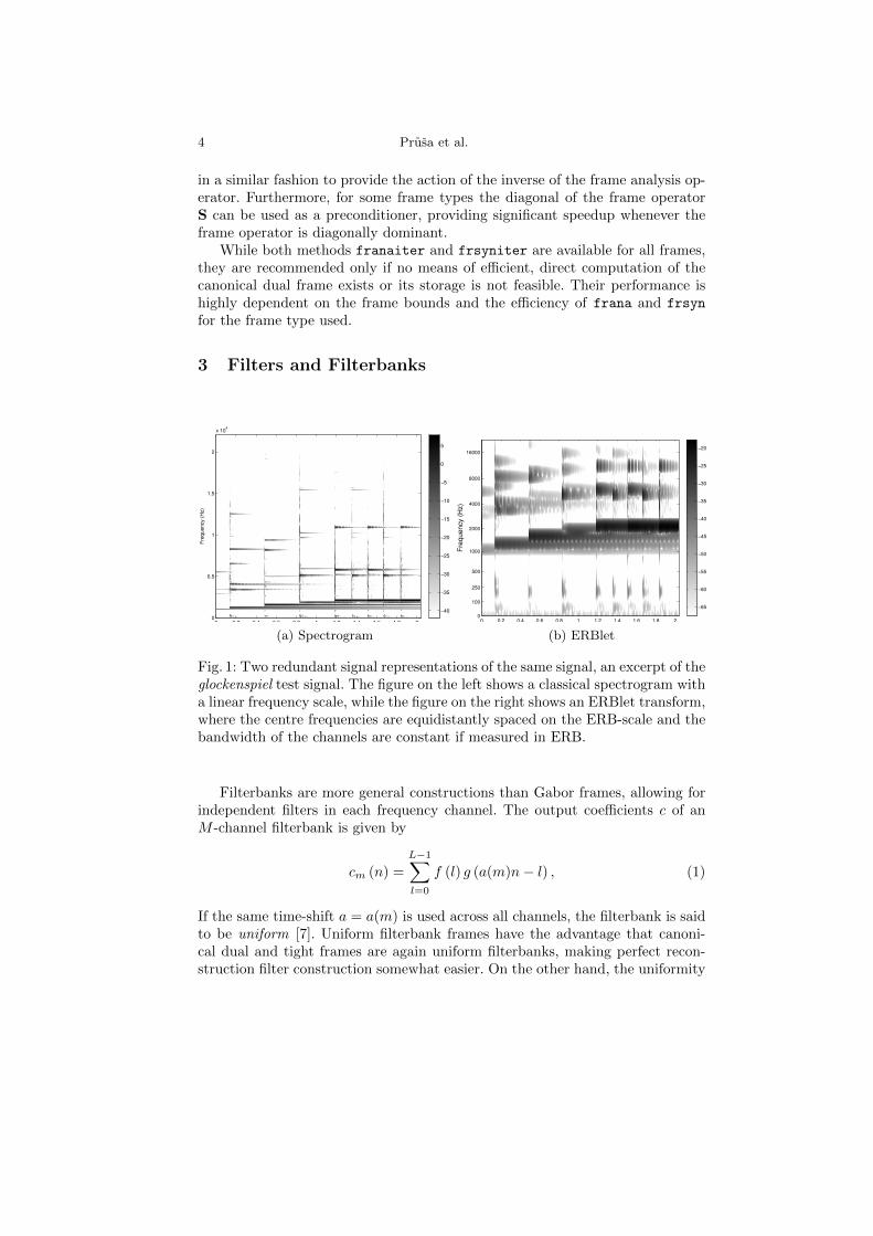
Fig. 1: Two redundant signal representations of the same signal, an excerpt of theglockenspiel test signal. The figure on the left shows a classical spectrogram witha linear frequency scale, while the figure on the right shows an ERBlet transform,where the centre frequencies are equidistantly spaced on the ERB-scale and thebandwidth of the channels are constant if measured in ERB.

Filterbanks are more general constructions than Gabor frames, allowing forindependent filters in each frequency channel. The output coefficients c of anM -channel filterbank is given by

cm (n) =

L−1∑l=0

f (l) g (a(m)n− l) , (1)

If the same time-shift a = a(m) is used across all channels, the filterbank is saidto be uniform [7]. Uniform filterbank frames have the advantage that canoni-cal dual and tight frames are again uniform filterbanks, making perfect recon-struction filter construction somewhat easier. On the other hand, the uniformity


usually means than too many coefficients are kept for subband channels with asmall bandwidth.

Another approach to filterbank inversion is to construct the filterbank in sucha way that it becomes a painless frame [10]. A painless frame has the propertythat its frame operator is a diagonal matrix. This makes it easy to find thecanonical dual and tight frames, and in the case of painless filterbanks theyare again painless filterbanks. A filterbank is painless if the filters are strictlybandlimited with a bandwidth (in radians) that is less than or equal to 2π/a(m).

In a general filterbank, the user must provide filters to cover the whole fre-quency axis, including the negative frequencies. For users working with real-valued signals only, a real filterbank construction exists in LTFAT. These con-structions work as if the filterbank was extended with the conjugates of the givenfilters. They work entirely similar as the real valued Gabor frames.

ERBlets [28] is a family of perfect reconstruction filterbanks with a frequencyresolution that follows the ERB-scale [19]. The ERBlets are included in LTFATthrough a routine that generates the correct filters and downsampling rates. Toaid researchers working with auditory signal processing, the toolbox containsa small collection of routines to generate the most common auditory scales,range compression and specialized auditory filters. An highly redundant ERBlet-representation of a common test signal is shown on Figure 1b, to create anauditory “spectrogram”.

4 Gabor Analysis: Linear Frequency Scales

The Discrete Gabor Transform (DGT) with M channels, time-shift of a andwindow function g ∈ CL is given by

c(m,n) =

L−1∑l=0

f (l) g (l − na) e−2πiml/M ,

where m = 0, . . . ,M−1 and n = 0, . . . , L/a. An overview of the theory of Gaborframes can be found in [21]. The toolbox supports two types of Gabor systems:the normal type dgt and a type dgtreal which only works for real-valued signals.This type of frame simply returns the coefficients of the positive frequencies inthe time-frequency plane. For practical applications it is a convenient way ofnot having to deal with the redundant information in the negative frequencies.An highly redundant DGT-representation of a common test signal is shown onFigure 1a, this is simply a normal spectrogram.

4.1 The Discrete Wilson Transform and the MDCT

The wilson frame type represents a type of time-frequency basis known as aWilson basis [12]. Wilson bases were proposed as substitutes for Gabor frames,because of the impossibility of constructing Gabor systems that would be simul-taneously generated using well-behaved windows, and bases of the consideredsignal spaces.

6 Prusa et al.

A Wilson basis is formed by taking linear combinations of appropriate basisfunctions from a Gabor frame with redundancy 2, [6]. Essentially Gabor atomsof positive and negative frequencies are combined, with suitable fine tuning oftheir phases. This remarkable construction turns a tight Gabor frame into anreal, orthonormal basis, or turns a non-tight Gabor frame into a Riesz basis(corresponding to a bi-orthogonal filterbank). In [25] this system is described asa “linear phase cosine modulated maximally decimated filter bank with perfectreconstruction”.

The MDCT (modified discrete cosine transform) is another substitute for thenon-existent well localised Gabor bases that has become extremely popular re-cently for its numerous applications, in audio coding for instance [27,31,30]. BothWilson and MDCT bases are variations of the same construction, the notabledifference being that the basis vectors of a Wilson basis with M channels arecentered on the M roots of unity in frequency, while the MDCT basis functionsare centered in between.

The coefficients c ∈ CM×N computed by the MDCT of f ∈ CL are given by:For m+ n even:

c (m,n) =√

2

L−1∑l=0

f(l) cos

(π

M

(m+

1

2

)l +

π

4

)g(l − na). (2)

For m+ n odd:

c (m,n) =√

2

L−1∑l=0

f(l) sin

(π

M

(m+

1

2

)l +

π

4

)g(l − na). (3)

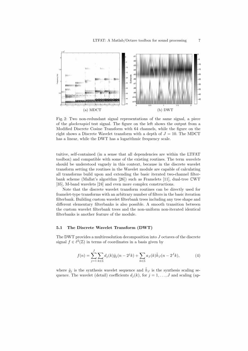
MDCT coefficients of a common test signal are shown on Figure 2a.

4.2 Adaptable Time Scale

Non-stationary Discrete Gabor Systems (NSDGS) [5] is a generalization of Ga-bor frames, where window and time-shift are allowed to change over time, butthe frequency channels are always placed on a linear scale (through the properapplication of a Discrete Fourier Transform).

Similar to filterbanks, an NSDGT must be either uniform or painless to ahave a fast linear reconstruction. A uniform NSDGS has the same frequencyresolution for all time-shifts and a painless NSDGT always has a window lengththat is less than or equal to the corresponding number of channels. In thesecases, the dual and tight systems are again NSDGTs. As for Gabor systems, thereal-valued NSDGT provides only the positive frequencies of the DFT.

NSDGTs are usefull for adapting the time and frequency resolution over time,for instance for tracking the pitch changes in a voice or musical signal.

5 Wavelet Analysis: Logarithmic Frequency Scale

The newly added wavelet module extends the one-dimensional time-frequencysignal processing capabilities of the toolbox. The module is intended to be in-


Time (s)

Fre

qu

en

cy (

Hz)

0 0.2 0.4 0.6 0.8 1 1.2 1.4 1.6 1.8 20

0.5

1

1.5

2

x 104

−45

−40

−35

−30

−25

−20

−15

−10

−5

0

(a) MDCTTime (s)

Su

bb

an

ds

0 0.5 1 1.5 2

a10

d10

d9

d8

d7

d6

d5

d4

d3

d2

d1

−45

−40

−35

−30

−25

−20

−15

−10

−5

0

(b) DWT

Fig. 2: Two non-redundant signal representations of the same signal, a pieceof the glockenspiel test signal. The figure on the left shows the output from aModified Discrete Cosine Transform with 64 channels, while the figure on theright shows a Discrete Wavelet transform with a depth of J = 10. The MDCThas a linear, while the DWT has a logarithmic frequency scale.

tuitive, self-contained (in a sense that all dependencies are within the LTFATtoolbox) and compatible with some of the existing routines. The term waveletsshould be understood vaguely in this context, because in the discrete wavelettransform setting the routines in the Wavelet module are capable of calculatingall transforms build upon and extending the basic iterated two-channel filter-bank scheme (Mallat’s algorithm [26]) such as Framelets [11], dual-tree CWT[35], M-band wavelets [24] and even more complex constructions.

Note that the discrete wavelet transform routines can be directly used forframelet-type transforms with an arbitrary number of filters in the basic iterationfilterbank. Building custom wavelet filterbank trees including any tree shape anddifferent elementary filterbanks is also possible. A smooth transition betweenthe custom wavelet filterbank trees and the non-uniform non-iterated identicalfilterbanks is another feature of the module.

5.1 The Discrete Wavelet Transform (DWT)

The DWT provides a multiresolution decomposition into J octaves of the discretesignal f ∈ `2(Z) in terms of coordinates in a basis given by

f(n) =

J∑j=1

∑k∈Z

dj(k)gj(n− 2jk) +∑k∈Z

aJ(k)hJ(n− 2Jk), (4)

where gj is the synthesis wavelet sequence and hJ is the synthesis scaling se-quence. The wavelet (detail) coefficients dj(k), for j = 1, . . . , J and scaling (ap-

8 Prusa et al.

proximation) coefficients aJ(k) are given by

dj(k) =∑n

f(n)g∗j (n− 2jk) (5)

andaJ(k) =

∑n

f(n)h∗J(n− 2Jk) (6)

respectively, where g∗j (n) is the complex conjugate of the analysis wavelet se-quence and h∗J(n) is the complex conjugate of the analysis scaling sequence. Theanalysis sequences are related in such a way that they are built from the twosuitably designed half-band elementary filters g1(n) (high-pass, also referred toas the discrete wavelet) and h1(n) (low-pass) as follows

hj+1(n) =∑k

hj(k)h1(n− 2k), (7)

gj+1(n) =∑k

gj(k)h1(n− 2k). (8)

The same procedure holds for the synthesis sequences but with the differentelementary filters g1(n) and h1(n). Perfect reconstruction is possible if the ele-mentary filters have been suitably designed. The equations (7),(8) are in fact anenabling factor for the well-known Mallat’s algorithm (also known as the fastwavelet transform). It comprises of an iterative application of the time-reversedelementary two-channel FIR filter bank followed by a factor of two subsampling

dj+1k(k) = (aj ∗ g1(· − n))↓2 (k), (9)

aj+1(k) = (aj ∗ h1(· − n))↓2 (k), (10)

make where ∗ is the convolution operation and a0 = f . The iterative applicationof the elementary filterbank forms a tree-shaped filterbank, where just the low-pass output is iterated on. The signal reconstruction from the coefficients is thendone by applying a mirrored filterbank tree using the synthesis filters g1(n) andh1(n).

In practice when f ∈ CL, the signal boundaries have to be taken into ac-count. Usually the periodic extension is considered (which means the convolu-tions (9),(10) are circular), which requires L to be an integer multiple of 2J . Inthis case, the number of coefficients is halved with each iteration and the overallcoefficient count is equal to L. The approach to considering any other extension(symmetric, zero-padding, etc.) exploits the fact that the filters are FIR andthus the information about the signal extensions can be saved in the additionalcoefficients. The coefficients are obtained by the full linear convolution with (nowcausal) filters. The resulting wavelet representation is called expansive becausethe number of coefficients at level j becomes Lj = b2−jL + (1 − 2−j)(m − 1)c[34], where m is the length of the filters, with no restrictions on L.

DWT coefficients of a common test signal are shown on Figure 2b.


5.2 General Filterbank Trees

The DWT is known to have several drawbacks. First, it is merely 2J -shift in-variant, which becomes a burden in denoising schemes. Secondly, the criticalsubsampling introduces aliasing which is supposed to be cancelled by the syn-thesis filterbank. Provided some modification of the coefficients has been done,the aliasing may no longer be compensated for. Finally, the octave frequency res-olution may not be enough for some applications. The first two shortcomings canbe avoided by the undecimated DWT with a cost of a high redundancy and thefrequency resolution may be improved by the use of the wavelet packets, whereon the other hand the aliasing is an even greater issue. Several modifications ofthe DWT filterbank tree were proposed to avoid the mentioned shortcomingsstill maintaining the wavelet filter tree structure but using different numbers ofthe elementary filters, adding parallel wavelet filter trees, alternating differentelementary filter sets etc. All these alternative constructions in both decimatedand undecimated versions are incorporated in the Wavelet module by means ofthe general filterbank tree framework.

The framework also encompasses building custom wavelet packets and waveletpacket subtrees, which differ from the DWT-shaped trees by allowing further re-cursive decomposition of the high-pass filter output creating possibly a full treefilterbank. The wavelet packet coefficients are outputs of each of the nodes inthe tree. Such a representation is highly redundant, but leaves of any admis-sible subtree form a basis. The best subtree (basis) search algorithm relies oncomparing the entropy of the wavelet packet coefficient subbands.

5.3 CQT

Additionally, LTFAT provides the method cqt for perfectly invertible constant-Q (CQ) filterbanks [22]. While conceptually reminiscent of Wavelet transforms,CQ techniques use a much higher number of channels per octave, resulting in amore detailed, redundant representation. The filters in a CQ transform are placedalong the frequency axis with a constant ratio of center frequency to bandwidth,or Q-factor. Particularly interesting for acoustic signal processing, they provide amuch finer frequency resolution than classical Wavelet techniques and harmonicstructures are left invariant under a shift across frequency channels.

6 Operations on Coefficients

6.1 Frame multipliers

A frame multiplier [4] is an operator constructed by multiplying frame coeffi-cients with a symbol m:

Mmf =

K−1∑k=0

mk 〈f, Ψak 〉ψsk,

10 Prusa et al.

time (seconds)

freq

uenc

y (H

z)

Glockenspiel − dB−scaled CQ−NSGT

0 1 2 3 4 5 50

200

800

3200

12800

22050

(a) CQT spectrogram of the test signal

time (seconds)

freq

uenc

y (H

z)

Mask

0 1 2 3 4 5 50

200

800

3200

12800

22050

(b) Symbol

time (seconds)

freq

uenc

y (H

z)

Glockenspiel (masked) − dB−scaled CQ−NSGT

0 1 2 3 4 5 50

200

800

3200

12800

22050

(c) Effect of the multiplier

time (seconds)

freq

uenc

y (H

z)

Glockenspiel component − dB−scaled CQ−NSGT

0 1 2 3 4 5 50

200

800

3200

12800

22050

(d) Effect of the multiplier using the inversesymbol.

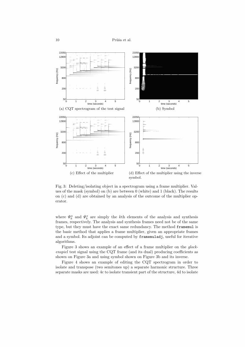
Fig. 3: Deleting/isolating object in a spectrogram using a frame multiplier. Val-ues of the mask (symbol) on (b) are between 0 (white) and 1 (black). The resultson (c) and (d) are obtained by an analysis of the outcome of the multiplier op-erator.

where Ψak and Ψsk are simply the kth elements of the analysis and synthesisframes, respectively. The analysis and synthesis frames need not be of the sametype, but they must have the exact same redundancy. The method framemul isthe basic method that applies a frame multiplier, given an appropriate framesand a symbol. Its adjoint can be computed by framemuladj, useful for iterativealgorithms.

Figure 3 shows an example of an effect of a frame multiplier on the glock-enspiel test signal using the CQT frame (and its dual) producing coefficients asshown on Figure 3a and using symbol shown on Figure 3b and its inverse.

Figure 4 shows an example of editing the CQT spectrogram in order toisolate and transpose (two semitones up) a separate harmonic structure. Threeseparate masks are used: 4c to isolate transient part of the structure, 4d to isolate


time (seconds)

freq

uenc

y (H

z)

Original Glockenspiel signal

0 0.5 1 1.5

200

800

3200

12800

(a) Detail of the CQT of the test signal

time (seconds)

freq

uenc

y (H

z)

CQ−NSGT modified signal

0 0.5 1 1.5

200

800

3200

12800

(b) Detail of the CQT of the result

time (seconds)

freq

uenc

y (H

z)

Sinusoidal mask

0 0.5 1 1.5 50

200

800

3200

12800

(c) Harmonic masktime (seconds)

freq

uenc

y (H

z)

Transient mask

0 0.5 1 1.5 50

200

800

3200

12800

(d) Transient masktime (seconds)

freq

uenc

y (H

z)

Remainder mask

0 0.5 1 1.5 50

200

800

3200

12800

(e) Remainder mask

time (seconds)

freq

uenc

y (H

z)

Extracted sinusoid

0 0.5 1 1.5 50

200

800

3200

12800

(f) Harmonic parttime (seconds)

freq

uenc

y (H

z)

Extracted transient

0 0.5 1 1.5 50

200

800

3200

12800

(g) Transient parttime (seconds)

freq

uenc

y (H

z)

Remainder signal

0 0.5 1 1.5 50

200

800

3200

12800

(h) Remainder

Fig. 4: Transposition of a single harmonic structure of the test signal glockenspiel.

harmonic part of the structure and 4e to remove the structure to be replacedwith the transposed version. The result of the masking operation is shown on4f, 4g and 4h respectively. The only modification done is a frequency shift ofthe harmonic part 4f by 8 bins upwards. The transient part is left as is to avoidphasing effects. The inverse transform is applied to the element-wise sum of thetransient, the remainder and the modified harmonic coefficients layers. The CQTspectrogram of the result is shown on 4b.

The CQT used in both examples was defined for the frequency range 50 Hz– 20 kHz with 48 bins per octave.

12 Prusa et al.

Sound examples can be found at http://ltfat.sourceforge.net/notes/

022.

6.2 Non-linear Analysis and Synthesis

Time (s)

Fre

quency (

Hz)

0 0.05 0.1 0.15 0.2 0.25 0.3 0.350

1000

2000

3000

4000

5000

6000

7000

8000

−40

−35

−30

−25

−20

−15

−10

−5

0

5

(a) Magnitude of coefficientsTime (s)

Fre

quency (

Hz)

0 0.05 0.1 0.15 0.2 0.25 0.3 0.350

1000

2000

3000

4000

5000

6000

7000

8000

0.5

1

1.5

2

2.5

3

(b) Phase difference

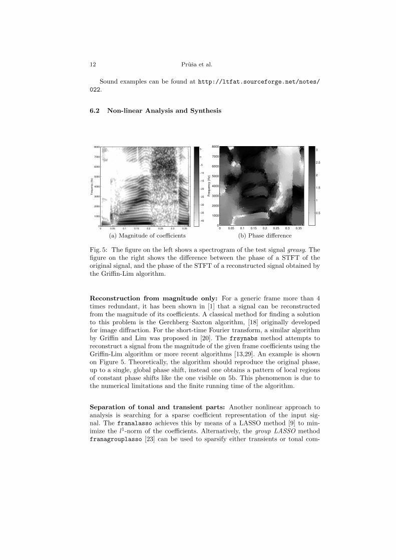
Fig. 5: The figure on the left shows a spectrogram of the test signal greasy. Thefigure on the right shows the difference between the phase of a STFT of theoriginal signal, and the phase of the STFT of a reconstructed signal obtained bythe Griffin-Lim algorithm.

Reconstruction from magnitude only: For a generic frame more than 4times redundant, it has been shown in [1] that a signal can be reconstructedfrom the magnitude of its coefficients. A classical method for finding a solutionto this problem is the Gerchberg–Saxton algorithm, [18] originally developedfor image diffraction. For the short-time Fourier transform, a similar algorithmby Griffin and Lim was proposed in [20]. The frsynabs method attempts toreconstruct a signal from the magnitude of the given frame coefficients using theGriffin-Lim algorithm or more recent algorithms [13,29]. An example is shownon Figure 5. Theoretically, the algorithm should reproduce the original phase,up to a single, global phase shift, instead one obtains a pattern of local regionsof constant phase shifts like the one visible on 5b. This phenomenon is due tothe numerical limitations and the finite running time of the algorithm.

Separation of tonal and transient parts: Another nonlinear approach toanalysis is searching for a sparse coefficient representation of the input sig-nal. The franalasso achieves this by means of a LASSO method [9] to min-imize the l1-norm of the coefficients. Alternatively, the group LASSO methodfranagrouplasso [23] can be used to sparsify either transients or tonal com-

http://ltfat.sourceforge.net/notes/022

http://ltfat.sourceforge.net/notes/022


Time (s)

Fre

quency (

Hz)

0 0.2 0.4 0.6 0.8 1 1.2 1.40

0.5

1

1.5

2

x 104

−40

−35

−30

−25

−20

−15

−10

−5

0

5

(a) Tonal partTime (s)

Fre

quency (

Hz)

0 0.2 0.4 0.6 0.8 1 1.2 1.40

0.5

1

1.5

2

x 104

−50

−45

−40

−35

−30

−25

−20

−15

−10

−5

(b) Transient part

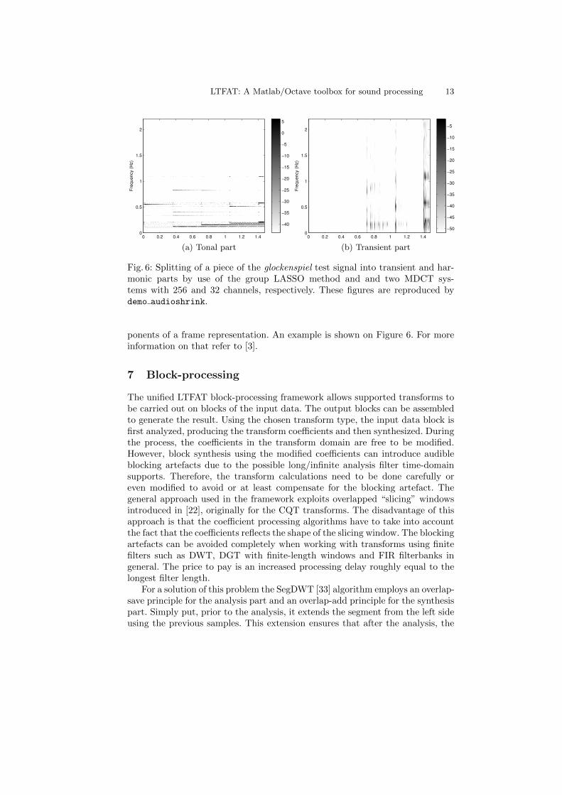
Fig. 6: Splitting of a piece of the glockenspiel test signal into transient and har-monic parts by use of the group LASSO method and and two MDCT sys-tems with 256 and 32 channels, respectively. These figures are reproduced bydemo audioshrink.

ponents of a frame representation. An example is shown on Figure 6. For moreinformation on that refer to [3].

7 Block-processing

The unified LTFAT block-processing framework allows supported transforms tobe carried out on blocks of the input data. The output blocks can be assembledto generate the result. Using the chosen transform type, the input data block isfirst analyzed, producing the transform coefficients and then synthesized. Duringthe process, the coefficients in the transform domain are free to be modified.However, block synthesis using the modified coefficients can introduce audibleblocking artefacts due to the possible long/infinite analysis filter time-domainsupports. Therefore, the transform calculations need to be done carefully oreven modified to avoid or at least compensate for the blocking artefact. Thegeneral approach used in the framework exploits overlapped “slicing” windowsintroduced in [22], originally for the CQT transforms. The disadvantage of thisapproach is that the coefficient processing algorithms have to take into accountthe fact that the coefficients reflects the shape of the slicing window. The blockingartefacts can be avoided completely when working with transforms using finitefilters such as DWT, DGT with finite-length windows and FIR filterbanks ingeneral. The price to pay is an increased processing delay roughly equal to thelongest filter length.

For a solution of this problem the SegDWT [33] algorithm employs an overlap-save principle for the analysis part and an overlap-add principle for the synthesispart. Simply put, prior to the analysis, it extends the segment from the left sideusing the previous samples. This extension ensures that after the analysis, the

14 Prusa et al.

obtained coefficients are exactly the ones one would get analyzing the whole in-put signal and picking up just those coefficients belonging to the processed block.Because of this feature, any coefficient processing algorithm can be applied withthe same impact as if the same algorithm was applied to coefficients withoutdividing the data into blocks at all. The reconstructed segments have the lengthof the extended analyzed ones and the overlapping parts are simply added. Asfor the SegDWT algorithm itself, the left extension length required prior to theanalysis of a given block is

L(Sn) = r(J) + (Sn mod 2J), (11)

where J stands for the number of the wavelet filterbank iterations, Sn for firstsample index of the segment n in the global point of view and r(J) = (2J −1)(m−2), where m is the wavelet filter length. Note that the SegDWT algorithmaccepts any block size s (up to a minimum length s = 2J) and the block sizescan even vary among each other. After processing the wavelet coefficients andapplication of the inverse Mallat’s algorithm, the last L(Sn + s) samples shouldbe saved to be added to the respective reconstructed samples of the followingblock. In case L(Sn + s) > s, additional and more complex buffering have to beemployed. The algorithm delay is r(J) samples for block lengths restricted tovalues s = k2J , k = 1, 2, 3, . . . and r(J) + 2J − 1 otherwise.

The LTFAT block-processing framework combined with suitable open-sourceaudio I/O libraries, like Portaudio http://www.portaudio.com/ and Playrechttp://www.playrec.co.uk/ allows for the true real-time audio stream pro-cessing in Matlab/Octave. The libraries provide interfaces for the cross-platformnon-blocking audio recording and playback. Such processing requires the trans-form routines to be fast enough to deliver the processed blocks on time to assuregapless playback. Not only for this purpose, many of the transforms included inLTFAT were implemented separately in C programming language.

An accompanying contribution [32], presented at this conference, demon-strates capabilities of the block-processing framework in the real-time setting.

References

1. Balan, R., Casazza, P., Edidin, D.: On signal reconstruction without phase. Appl.Comput. Harmon. Anal. 20(3), 345–356 (2006)

2. Balazs, P.: Frames and finite dimensionality: Frame transformation, classificationand algorithms. Applied Mathematical Sciences 2(41–44), 2131–2144 (2008)

3. Balazs, P., Dorfler, M., Kowalski, M., Torresani, B.: Adapted and adaptive lineartime-frequency representations: a synthesis point of view. IEEE Signal ProcessingMagazine (special issue: Time-Frequency Analysis and Applications) to appear, –(2013)

4. Balazs, P.: Basic definition and properties of Bessel multipliers. Journal of Math-ematical Analysis and Applications 325(1), 571–585 (January 2007)

5. Balazs, P., Dorfler, M., Holighaus, N., Jaillet, F., Velasco, G.: Theory, implemen-tation and applications of nonstationary Gabor frames. Journal of Computationaland Applied Mathematics 236(6), 1481–1496 (2011)

http://www.portaudio.com/

http://www.playrec.co.uk/


6. Bolcskei, H., Feichtinger, H.G., Grochenig, K., Hlawatsch, F.: Discrete-time Wil-son expansions. In: Proc. IEEE-SP 1996 Int. Sympos. Time-Frequency Time-ScaleAnalysis (june 1996)

7. Bolcskei, H., Hlawatsch, F., Feichtinger, H.G.: Frame-theoretic analysis of over-sampled filter banks. Signal Processing, IEEE Transactions on 46(12), 3256–3268(2002)

8. Christensen, O.: Frames and Bases. An Introductory Course. Applied and Numer-ical Harmonic Analysis. Basel Birkhauser (2008)

9. Daubechies, I., Defrise, M., De Mol, C.: An iterative thresholding algorithm forlinear inverse problems with a sparsity constraint. Communications in Pure andApplied Mathematics 57, 1413–1457 (2004)

10. Daubechies, I., Grossmann, A., Meyer, Y.: Painless non-orthogonal expansions. J.Math. Phys. 27, 1271–1283 (1986)

11. Daubechies, I., Han, B., Ron, A., Shen, Z.: Framelets: MRA-based constructionsof wavelet frames. Applied and Computational Harmonic Analysis 14(1), 1 – 46(2003)

12. Daubechies, I., Jaffard, S., Journe, J.: A simple Wilson orthonormal basis withexponential decay. SIAM J. Math. Anal. 22, 554–573 (1991)

13. Decorsiere, R., Søndergaard, P.L., MacDonald, E.N., Dau, T.: Optimization Ap-proach to the Reconstruction of a Signal from a Spectrogram-Like Representation.IEEE Trans. Acoust. Speech Signal Process. (submitted, 2013)

14. Dolson, M.: The phase vocoder: a tutorial. Computer Musical Journal 10(4), 11–27(1986)

15. Duffin, R.J., Schaeffer, A.C.: A class of nonharmonic Fourier series. Trans. Amer.Math. Soc. 72, 341–366 (1952)

16. Feichtinger, H.G., Strohmer, T. (eds.): Gabor Analysis and Algorithms.Birkhauser, Boston (1998)

17. Flandrin, P.: Time-Frequency/Time-Scale Analysis. Academic Press, San Diego(1999)

18. Gerchberg, R.W., Saxton, W.O.: A practical algorithm for the determination ofthe phase from image and diffraction plane pictures. Optik 35(2), 237–250 (1972)

19. Glasberg, B.R., Moore, B.: Derivation of auditory filter shapes from notched-noisedata. Hearing Research 47(1-2), 103 (1990)

20. Griffin, D., Lim, J.: Signal estimation from modified short-time Fourier transform.IEEE Trans. Acoust. Speech Signal Process. 32(2), 236–243 (1984)

21. Grochenig, K.: Foundations of Time-Frequency Analysis. Birkhauser (2001)22. Holighaus, N., Dorfler, M., Velasco, G.A., Grill, T.: A framework for invertible, real-

time constant-Q transforms. IEEE Transactions on Audio, Speech and LanguageProcessing 21(4), 775 –785 (2013)

23. Kowalski, M.: Sparse regression using mixed norms. Appl. Comput. Harmon. Anal.27(3), 303–324 (2009)

24. Lin, T., Xu, S., Shi, Q., Hao, P.: An algebraic construction of orthonormal M-band wavelets with perfect reconstruction. Applied mathematics and computation172(2), 717–730 (2006)

25. Lin, Y.P., Vaidyanathan, P.: Linear phase cosine modulated maximally decimatedfilter banks with perfectreconstruction. IEEE Trans. Signal Process. 43(11), 2525–2539 (1995)

26. Mallat, S.G.: A theory for multiresolution signal decomposition: The wavelet rep-resentation. IEEE Trans. Pattern Anal. Mach. Intell. 11(7), 674–693 (Jul 1989)

27. Malvar, H.S.: Signal Processing with Lapped Transforms. Artech House Publishers(1992)

16 Prusa et al.

28. Necciari, T., Balazs, P., Holighaus, N., Søndergaard, P.L.: The ERBlet transform:An auditory-based time-frequency representation with perfect reconstruction. In:Proceedings of the 38th International Conference on Acoustics, Speech, and SignalProcessing (ICASSP 2013). pp. 498–502. IEEE, Vancouver, Canada (May 2013)

29. Perraudin, N., Balazs, P., Søndergaard, P.L.: A fast Griffin-Lim algorithm. In:Proceedings of the IEEE Workshop on Applications of Signal Processing to Audioand Acoustics (WASPAA) (2013)

30. Princen, J.P., Johnson, A.W., Bradley, A.B.: Subband/transform coding using fil-ter bank designs based on time domain aliasing cancellation. Proceedings - ICASSP,IEEE International Conference on Acoustics, Speech and Signal Processing pp.2161–2164 (1987)

31. Princen, J.P., Bradley, A.B.: Analysis/synthesis filter bank design based on timedomain aliasing cancellation. IEEE Transactions on Acoustics, Speech, and SignalProcessing ASSP-34(5), 1153–1161 (1986)

32. Prusa, Z., Søndergaard, P.L., Balazs, P., Holighaus, N.: Real-Time Audio Pro-cessing in the Large Time Frequency Analysis Toolbox (2013), to be presentedat 10th International Symposium on Computer Music Multidisciplinary Research(CMMR)

33. Prusa, Z.: Segmentwise Discrete Wavelet Transform. Ph.D. thesis, Brno Universityof Technology, Brno (2012)

34. Rajmic, P., Prusa, Z.: Discrete Wavelet Transform of Finite Signals: Detailed Studyof the Algorithm. submitted (2013)

35. Selesnick, I., Baraniuk, R., Kingsbury, N.: The dual-tree complex wavelet trans-form. Signal Processing Magazine, IEEE 22(6), 123 – 151 (nov 2005)

36. Søndergaard, P.L., Torresani, B., Balazs, P.: The Linear Time Frequency AnalysisToolbox. International Journal of Wavelets, Multiresolution Analysis and Informa-tion Processing 10(4) (2012)

A Matlab/Octave toolbox for sound processing - LTFAT

Documents