A macroeconomic model for resource allocation in large-scale distributed systems

A Macroeconomic Model for Resource Allocation in

Large-Scale Distributed Systems

Xin Bai a, Dan C. Marinescu a,∗, Ladislau Boloni a,

Howard Jay Siegel b, Rose A. Daley c, I-Jeng Wang c

aSchool of Electrical Engineering and Computer Science

University of Central Florida, Orlando, FL 32816-2362

bDepartment of Electrical and Computer Engineering

and Department of Computer Science

Colorado State University, Fort Collins, CO 80523-1373

cApplied Physics Laboratory

Johns Hopkins University, 11100 Johns Hopkins Road Laurel, MD 20723-6099

Preprint submitted to Elsevier Science 16 March 2007

Abstract

In this paper we discuss an economic model for resource sharing in large-scale distributed

systems. The model captures traditional concepts such as consumer satisfaction and provider

revenues and enables us to analyze the effect of different pricing strategies upon measures

of performance important for the consumers and the providers. We show that given a par-

ticular set of model parameters the satisfaction reaches an optimum; this value represents

the perfect balance between the utility and the price paid for resources. Our results confirm

that brokers play a very important role and can influence positively the market. We also

show that consumer satisfaction does not track the consumer utility, these two important

performance measures for consumers behave differently under different pricing strategies.

Pricing strategies also affect the revenues obtained by providers, as well as, the ability to

satisfy a larger population of users.

Key words: Resource Allocation, Macroeconomic Model, Utility, Price, Consumer

Utility, Consumer Satisfaction, Large-Scale Distributed System

∗ Corresponding author. Phone: (407)8234860 FAX: (407)8235419Email address: [email protected] (Dan C. Marinescu).

2

1 Introduction and Motivation

Computational, service, and data grids, peer-to-peer systems, and ad-hoc wireless networks

are examples of open systems. Individual members of the community contribute computing

cycles, storage, services, and communication bandwidth to the pool of resources available to

the entire community; resources as well as consumers of resources could belong to different

administrative domains. In this case it is difficult to devise global resource allocation policies

and there is no central authority to enforce global policies and schedules. The existence of

multiple administrative domains is a reality in the Grid environments and the Internet. In the

context of our research, each administrative domain corresponds to a different organization

and has complete control of its resources and dictates the price and the amount of resources

available. A broker mediates between producers and consumers in different administrative

domains. The research reported in this paper investigates the use of macroeconomic models

for resource allocation in heterogeneous, distributed computing and communication systems.

Market-oriented economies have proved their advantages over alternative means to control

and manage resource allocation in social systems [8]. It seems reasonable to adapt some of

the successful ideas of economical models to resource allocation in large-scale computing

systems and to study market-oriented resource allocation algorithms. As shown by recent

studies, economic models are attractive for resource providers, beneficial for the consumers

of resources, and have societal benefits for large-scale distributed systems [41–43]. Fewer

resources are wasted, while excess capacity and overloading are averaged over a very large

number of providers and consumers. The system is more scalable and decision-making is dis-

tributed. In an economic model, all participants are considered self-interested. The resource

providers are trying to maximize their revenues. The consumers want to obtain the maximum

possible resources for the minimum possible price. The large number of participants makes

one-to-one negotiations expensive and unproductive.

3

In 1933 the Norwegian economist and Nobel laureate Ragnar Frisch introduced the di-

chotomy macroeconomy/microeconomy [16]. Macroeconomics deals with the economy as

a whole and studies aggregate trends such as total consumption and production [36], while

microeconomics is primarily focused on the economic behavior of individual units and the

role of prices in allocation of scarce resources [39]. While in our model we simulate the

individual customers and producers, the objectives are to improve the aggregate utility and

satisfaction of the entire user population and all the resources of the distributed system. Thus,

it seems more appropriate to call it a macroeconomic model.

The model presented in this paper is based upon concepts borrowed from economics, such

as utility and consumer satisfaction. Informally, utility quantifies the benefits obtained as

the result of being granted a certain amount of resources. Utility-based resource allocation

models have proved their potential in a different context, e.g., when the only resource is

the radio bandwidth, the size of the population is limited, and each participant has a unique

role (e.g., is a consumer) [4]. The heterogeneity of a large-scale distributed system, the large

spectrum of resources and demands placed upon these resources, the scale of the system,

the autonomy of individual resource providers, and the dual role of individual actors, as

consumer of some resources and provider for others, add complexity to the models we study

in this paper.

Different utility functions can be considered; a utility function should be: (i) monotonically

increasing with the amount of allocated resource; (ii) convex for high resource values; and

(iii) fast growing for small amounts of allocated resources. Increasing the resource allocation

will yield lower and lower increase in utility. Intuitively, this is justified by Amdalh’s law:

once a resource is plentiful, the performance bottleneck moves to another type of resource,

and adding additional resource yields little benefit. These observations lead us to conclude

that the utility function will have an S-shaped, sigmoid curve. Sigmoid functions have all

the desirable properties and have been used in many economic models, in biology, and some

4

other areas, as we discuss in Section 3.

In our model, each resource is characterized by a vector with several components. In the

general case, a request may require multiple resources or resources with multiple attributes

thus, more general utility functions are surfaces in hyperspaces with several dimensions. A

discussion of the relative advantages of different families of utility functions is an important

and timely subject, but beyond the scope of this paper. While the sigmoid is selected for us

here, it could be replaced by other functions within the framework of our model.

We define a measure of consumer’s satisfaction that takes into account the utility resulting

from resource consumption and the price paid by the consumer. We show that given a partic-

ular set of model parameters the satisfaction reaches an optimum; this value represents the

perfect balance between the utility and the price paid for resources.

Consumer satisfaction is a more general metric than QoS that typically refers to a single

performance measure (e.g., time to completion or end-to-end delay), and does not reflect

pricing. Moreover, QoS requirements are generally specified by an upper bound (e.g., the

jitter should be less than m milliseconds), while one can provide a continuous function de-

scribing the utility and select a provider that optimizes the satisfaction value, or one that is

very close to the optimum.

We also show that consumer satisfaction does not track the consumer utility; these two impor-

tant performance measures for consumers behave differently under different pricing strate-

gies. Pricing strategies also affect the revenues obtained by providers, as well as the request

acceptance ratio. We introduce three pricing policies and investigate the effect of several pa-

rameters upon critical measures of performance for producers and consumers. The pricing

policies are affected by the relationship between the amount of resources required and the

total amount we pay for them, as well as the overall state of the system. We analyze the case

when the price per unit is constant regardless of the amount of resources consumed (linear

5

pricing); pricing to encourage consumption, i.e., the more resources are used the lower be-

comes the average unit price (sub-linear pricing); and pricing to discourage consumption, i.e.,

the more resources are used the higher becomes the average unit price (super-linear pricing).

We also analyze the effect of resource abundance upon pricing strategies.

We foresee an adaptive and intelligent user behavior based upon the idea that, in the general

case, the same goal may be achieved through different means. We suggest the transformation

of imperative requests into elastic ones that reflect the level of utility. Practically, we specify

a range of target systems, e.g,, clusters with 100 to 10, 000 nodes, and for each potential target

of an elastic request we compute a satisfaction value and choose the one leading to the largest

satisfaction. Assume that we process a very large number of images and could use a variety

of system configurations each with its own utility and the corresponding satisfaction value.

Our best option is to use a cluster with 10, 000 nodes with 4 GB of memory per node, but

there are only a few such systems; at the other extreme, we could use a cluster more likely to

be available soon with only 100 nodes and 2 GB of main memory per node, but the execution

time would increase by four orders of magnitude. An elastic request quantifies the urgency

of the request and allows the broker and/or the user to compare the satisfaction values and

decide whether to pay a higher price for a unique resource, or use a readily available one.

Several models including ours include middlemen to mediate access to resources a strategy

rather common for agent systems. The role of a broker is to reconcile the selfish objectives

of individual resource providers and consumers with some global, societal objectives, e.g.,

to maximize the resource utilization of the system.

The best analogy for a broker in our model is a financial advisor in the real world. Clients

trust their financial advisors and disclose their financial objectives (corresponding to the

utility and satisfaction functions) to them. At the same time, the clients know and accept

the fact that the financial advisor will act in the context of existing laws and stock market

6

regulations, thus, it also serves societal objectives.

Most macroeconomic models include policy makers that establish societal objectives. For

example the Federal Reserve Board establishes monetary policies in the US and there are

counterparts in other countries. In a global economy the policy makers sometimes coordinate

their behavior. In the future our simulation studies should be extended to include policy

makers and multiple brokers.

Our results confirm that brokers play a very important role and can influence positively the

market. The development of broker-to-broker coordination models and an analysis of a more

complex system is well beyond the scope of this paper due to the complexity of the analysis

and space limitations. As expected, even with a set of simplifying assumptions, the models

are extremely complex and can only be evaluated through simulation.

The contributions of this paper are: (i) a macroeconomic model that includes policy makers

whose role is to establish societal objectives, trusted middleman whose role is to ensure

maximum satisfaction to their clients, and producers and consumers of resources; (ii) utility

and satisfaction functions, as well as pricing policies; (iii) a simulation study of the behavior

of a system with a single broker.

The paper is organized as follows: we survey different economic models applied to infor-

mation systems in Section 2 and compare their features with our model. In Section 3, we

introduce the basic elements of our model and define utility and satisfaction function, as well

as pricing strategies. The role of the middlemen is discussed in Section 4 and the results of a

simulation study are analyzed in Section 5; finally, we present our conclusions in Section 6.

7

2 Related Work

The development of the first global macroeconomic model, the Wharton Econometric Fore-

casting Associates LINK project, started in 1968 under the leadership of Nobel laureate

Lawrence Klein [30]. There are two basic analytical approaches to classical macroeconomics:

(a) Keynesian economics focused on demand and (b) supply-side economics focused on sup-

ply.

Interestingly enough, the most complex information system ever conceived, the Internet,

takes advantage of ideas that can be traced back to macroeconomics. While the Internet

is based upon a best effort service model, supply-side economics are reflected by over-

provisioning, namely building an excess bandwidth to ensure some levels of QoS.

Frank Kelly developed in late 1990s an analytical model for a self-managed Internet based

upon utility and cost [25]. Kelly considers a set of sessions s ∈ S that use a set of links l ∈ L;

each link l has a capacity C. If Ls is the set of links used by session s, then Us(rs), S ∈Ls) is a strictly concave, increasing function of the packet source rate, rs. He attempts to

maximize system utility with the constraint that the total bandwidth used on each link by

all connections is lower than the link capacity. If ps is the price function of the rate, then a

distributed algorithm solves a greedy optimization problem for every session:

max Us(rs)− psrs.

It turns out that the adaptive congestion control mechanism introduced in early 1980s for

TCP can be well described by Kelly’s model developed in late 1990s; the price in this case

is the probability of losing packets and the utility is a simple function of the round trip time

(RTT).

8

Extending Kelly’s model to a large-scale distributed system consisting of a collection of

heterogeneous systems, while feasible, would be rather impractical; the need to differentiate

services for individual consumers and specify a different utility function for each one of

them, the variety of prices and the fact that individual entities are consumers and providers at

the same time, makes such an extension very hard and possibly infeasible computationally.

Even though theoretical studies of economic models applied to information systems are only

now beginning to emerge, several companies including IBM (E-Business On Demand [23]),

HP (Adaptive Enterprise [22]), Sun Microsystems (pay-as-you-go [38]), as well as startups

such as Entropia, ProcessTree, Popular Power, Mojo Nation, United Devices, and Parabon

are embedding economics into their resource allocation systems. Economic concepts and

ideas are used for distributed storage systems such as the Stanford Peers Initiative [14] and

GnuNet [19] and distributed databases [3,37]. Java Market [2], JaWS [26], Xenoservers [31],

and others apply economic models for computer services.

The economic concepts and strategies embedded in existing or proposed systems and models

[11] are summarized in Table 1 and surveyed below. An auction starts with owners announc-

ing resources and inviting bids; consumers bid and the winner gets access to the resource.

In an English auction, when no bidder is willing to increase the bid, the auction ends and

the highest bidder wins; in first-price sealed-bid auction, every bidder submits a sealed-bid

and the highest bidder wins; in a Vickrey auction, every bidder submits a sealed-bid and the

highest bidder wins at the price of the second highest bidder; a Dutch auction starts with

a high price lowered until a bidder is willing to pay the current price. In bid-based pro-

portional resource sharing the percentage of resources allocated is a function of user’s bid

relative to others. Bargaining requires direct negotiations between producers and consumers

until they reach a mutually agreeable price. Bartering is conducted among the members of

a community that share each other’s resources. In commodity markets, providers advertise

their resource prices and charge users based on the amount of resources used; posted price

9

Table 1

Economic concepts and strategies in different systems. Abbreviations: Au - Auction; Ba - Bargain-

ing; Bt - Bartering; Cm - Commodity market; Co - Coalition; Mo - Monopoly; Ut -Utility; Cs -

Consumer satisfaction; Pr - Pricing policy; Results - performance results reported in literature, Ana-

litical/Simulation.

System Au Ba Bt Cm Co Mo Ut Cs Pr Results

ContractNet [35] Yes Yes No Yes No No No No No Deployed

Condor [13] No No No Yes No No No No Yes Deployed

Enhanced MOSIX [1] No No No No No No Yes No Yes Simulated

Mariposa [27] (based on

the Contract Net)

Yes Yes No Yes No No No No No Prototype

Rexec/Anemone [12] No No No Yes No Yes No No Yes Prototype

SETI@home [32] No No No Yes No No No No No Deployed

Spawn [41] Yes No No No No No Yes No Yes Prototype

Sun [38]) No No No Yes No No No No No Deployed

Our model No No No No No No Yes Yes Yes Simulation

allows providers to advertise special offers to attract consumers. In case of a monopoly, one

or a small number of resource providers decide a non-negotiable the price. Pricing policy

could be based on a flat fee, the resource usage duration, the subscription, the demand and

supply [28], or could be designed to encourage or discourage consumption.

Arguments that commodities markets are better choices for controlling grid resources than

auction strategies are presented in [42,43] based upon concepts such as price stability, market

equilibrium, consumer efficiency, and provider efficiency. An approach to implement auto-

matic selection of multiple negotiation models to adapt to the computation needs and changes

in a resource environment is discussed in [33]. A task-oriented mechanism for measuring the

economic value of using heterogeneous resources as a common currency is analyzed in [20];

resource consumers can compare the advantage of participating in a computational grid with

10

the alternative of purchasing their own resources necessary, and resource providers can eval-

uate the profit of putting their resources into a grid. A comparative analysis of market-based

resource allocation by continuous double auctions and by the proportional share protocol

versus a conventional round-robin approach is presented in [18]. A game theoretic pricing

strategy for efficient job allocation in mobile grids is discussed in [17]; a grid resource allo-

cation model based upon a game theoretic approach is presented in [24].

Table 1 summarizes the key features of a variety of economic-based systems for resource

allocation. Our approach differs from other models in that it is based upon utility and satis-

faction functions and pricing policies.

3 Basic Concepts

An efficient and fair utilization of the resources can be obtained only through a scheme that

gives incentives to the providers to share their resources and that encourages the consumers

to maximize the utility of the received resources. A well-tested model for such a scheme is

based on an economic model, in which the resources need to be paid for in a real or virtual

currency. This model has the advantage of being provably scalable, and we can successfully

reuse or adapt the models that govern the economy in our society.

To study possible resource management policies, we have to develop resource consump-

tion models that take into account different, possibly contradictory, views of the benefits

associated with resource consumption as well as the rewards for providing resources to the

consumer population. Such models tend to be very complex and only seldom amenable to

analytical solutions.

In this section we introduce the basic concepts and notations for our model. First, we in-

troduce price, utility, and satisfaction functions; then we present our resource provider-

11

consumer model. To capture the objectives of the entities involved in the computational

economy we use: (i) a consumer utility function, 0 ≤ u(r) ≤ 1, to represent the utility

provided to an individual consumer, where r represents the amount of allocated resource; (ii)

a provider price function, p(r), imposed by a resource provider, and (iii) a consumer satisfac-

tion function, s(u(r), p(r)), 0 ≤ s ≤ 1, to quantify the level of satisfaction; the satisfaction

depends on both the provided utility and the paid price.

3.1 Price Functions

0 r

p(r)

super-linear

linear

sub-linear

max

min

TL TH

(a) (b)

Fig. 1. (a) Sub-linear, linear, and super-linear price functions. (b) The unit price varies with ρ, the load

index of the provider.

We discuss the three pricing functions in Figure 1(a). Given the constant, ξ, the three partic-

ular pricing functions we choose are:

(a) The price per unit is constant regardless of the amount of resources consumed (linear

pricing):

p(r) = ξ · r (1)

(b) Discourage consumption: the more resources are used, the higher becomes the average

12

unit price (super-linear pricing):

p(r) = ξ · rd (2)

where d > 1. For this equation, we use d = 1.5 throughout the remainder of the paper.

(c) Encourage consumption: the more resources are used, the lower becomes the average unit

price (sub-linear pricing):

p(r) = ξ · re (3)

where e < 1. For this equation, we use e = 0.5 throughout the remainder of the paper.

We also analyze the effect of resource abundance; in this case we define the load index

ρ as the ratio of total amount of allocated resources to the capacity of the provider and

consider three regions: low, medium, and high load index. We denote the low, medium, and

high regions as the interval of [0, ρTL), [ρTL, ρTH ], and (ρTH , 1], respectively, as shown in

Figure 1(b). The pricing strategy for each region is different. We consider two models, EDL -

Encourage/Discourage Linear, and EDN - Encourage/Discourage Nonlinear. The choice of

the ρTL, ρTH is basically a policy decision. However, in order to have the desired influence

on the system as a whole, the three intervals need to be of a sufficient size. Values such as

ρTL = 0.49 and ρTH = 0.51 make the target interval unreasonably small; very low ρTL and

very high ρTH values make the pricing strategy degenerate into a constant price strategy. The

values used throughout this paper are ρTL = 0.3 and ρTH = 0.7.

For the first model, the unit price is constant in each region, but different in different re-

gions, as defined in Equation 4, and shown in Figure 1(b). We introduce three prices, each

corresponding to a range of the system load: minimal, ξmin, maximal, ξmax, and ξ, the price

corresponding to medium load. For low load the providers use lower prices to encourage

resource consumption, but do not lower the price below ξmin. For high load, the providers

gradually increase the price, up to ξmax. The choice of the ξmin and ξmax are a matter of

policy, however, too low values for ξmin would make resources basically free for nodes with

13

low utilization, and very high values of ξmax would make resources too expensive. We used

the values of ξmax = 2× ξ, and ξmin = 0.5× ξ throughout the remainder of the paper.

p(r) =

(ξmin + ρ

ρTL(ξ − ξmin)

)· r if ρ ∈ [0, ρTL);

ξ · r if ρ ∈ [ρTL, ρTH ];

(ξ + ρ−ρTH

1.0−ρTH(ξmax − ξ)

)· r if ρ ∈ (ρTH , 1.0].

(4)

For the second model, when ρ is low, the provider uses a sub-linear price function; when ρ

is high, the provider uses a super-linear price function; otherwise, the provider uses a linear

price function, as expressed by Equation 5:

p(r) =

ξ · re if ρ ∈ [0, ρTL);

ξ · r if ρ ∈ [ρTL, ρTH];

ξ · rd if ρ ∈ (ρTH , 1.0].

(5)

where e < 1 and d > 1. The choice of e and d follow similar considerations like the choice of

parameters for the EDL model: we need to encourage and discourage the customers, while

still maintaining the prices in a justifiable range. In this paper we are using the values of

e = 0.5 and d = 1.5, which provide an appropriate range of prices.

3.2 Utility Function

The utility function should be a non-decreasing function of r, i.e., we assume that the more

resources are allocated to the consumer, the higher the consumer utility is. However, when

enough resources have been allocated to the consumer, i.e., some threshold is reached, an

increase of allocated resources would bring no improvement of the utility. On the other hand,

14

if the amount of resources is below some threshold the utility is extremely low. Thus, we

expect the utility to be a concave function and reach saturation as the consumer gets all the

resources it can use effectively. These conditions are reflected by the following equations:

du(r)

dr≥ 0, lim

r→∞du(r)

dr= 0 (6)

For example, if a parallel application could use at most 100 nodes of a cluster, its utility

reflected by a utility function does not increase if its allocation increases from 100 to 110

nodes. If we allocate less than 10 nodes then the system may spend most of its time paging

and experiencing cache misses and the execution time would be prohibitively high.

Different functions can be used to model this behavior and we choose one of them, a sigmoid:

u(r) =(r/ω)ζ

1 + (r/ω)ζ (7)

where ζ and ω are constants provided by the consumer, ζ ≥ 2, and ω > 0. Clearly, 0 ≤u(r) < 1 and u(ω) = 1/2.

0

1

r

u

StartingPhase

MaturingPhase

AgingPhase

0.0

1.0

r

s

Low Unit PriceMedium Unit Price

High Unit Price

(a) (b)

Fig. 2. (a) A sigmoid is used to model the utility function; a sigmoid includes three phases: the

starting phase, the maturing phase, and the aging phase. (b) The satisfaction function for a sigmoid

utility function and three linear price functions with low, medium, and high unit price.

A sigmoid is a tilted S-shaped curve that could be used to represent the life-cycles of living,

15

as well as man-made, social, or economical systems. It has three distinct phases: an incipient

or starting phase, a maturing phase, and a declining or aging phase, as shown in Figure 2(a).

3.3 Satisfaction Function

A consumer satisfaction function takes into account both the utility provided to the consumer

and the price paid for the resources. For a given utility, the satisfaction function should in-

crease when the price decreases and, for a given price, the satisfaction function should in-

crease when the utility u increases. These requirements are reflected by Equation (8).

∂s

∂p≤ 0,

∂s

∂u≥ 0 (8)

Furthermore, a normalized satisfaction function should satisfy the following conditions:

• the degree of satisfaction, s(u(r), p(r)), for a given price p(r), approaches the minimum,

0, when the utility, u(r), approaches 0;

• the degree of satisfaction, s(u(r), p(r)), for a given price p(r), approaches the maximum,

1, when the utility, u(r), approaches infinity;

• the degree of satisfaction, s(u(r), p(r)), for a given utility u(r), approaches the maximum,

1, when the price, p(r), approaches 0; and

• the degree of satisfaction, s(u(r), p(r)), for a given utility u(r), approaches the minimum,

0, when the price, p(r), approaches infinity.

These requirements are reflected by Equations (9) and (10).

∀p > 0, limu→0

s(u, p) = 0, limu→∞ s(u, p) = 1 (9)

∀u > 0, limp→0

s(u, p) = 1, limp→∞ s(u, p) = 0 (10)

16

A candidate satisfaction function is [39]:

s(u, p) = 1− e−κ·uµ·p−ε

(11)

where κ, µ, and ε are appropriate positive constants. The satisfaction function based upon

the utility function in Equation 7 is normalized; given a reference price φ we consider also a

normalized price function and we end up with a satisfaction function given by:

s(u, p) = 1− e−κ·uµ·(p/φ)−ε

. (12)

Because u and p are functions of r, satisfaction increases as more resources are allocated,

reaches an optimum, and then declines, as shown in Figure 2(b). The optimum satisfaction

depends upon the pricing strategy; not unexpectedly, the higher the unit price, the lower the

satisfaction.

The 3D surfaces representing the relationship s = s(r, ξ) between satisfaction s and the unit

price ξ and amount of resources r for several pricing functions (super-linear, linear, and sub-

linear) are presented in Figure 3. As we can see from the cut through the surfaces s = s(r, ξ)

at a constat ξ when we discourage consumption (super-linear pricing) the optimum satisfac-

tion is lower and occurs for fewer resources; when we encourage consumption (sub-linear

pricing) the optimum satisfaction is improved and occurs for a larger amount of resources.

These plots reassure us that the satisfaction function has the desired behavior.

3.4 Resource Provider-Consumer Model

Consider a system with n providers offering computing resources and m consumers. To

simplifying the model, we assume that the two sets are disjoint. Call U the set of consumers

and R the set of providers. The n providers are labeled 1 to n and the m consumers are

17

02

46

8100

1

2

3

0

0.2

0.4

0.6

0.8

1

rξ

s

02

46

8100

1

2

3

0

0.2

0.4

0.6

0.8

1

rξ

s

(a) (b)

02

46

8100

1

2

3

0

0.2

0.4

0.6

0.8

1

rξ

s

0 0.1 0.2 0.3 0.4 0.5 0.6 0.7 0.8 0.9

1

0 1 2 3 4 5

s

r

SuperlinearLinear

Sublinear

(c) (d)

Fig. 3. The relationship between satisfaction s and the unit price ξ and amount of resources r. The

satisfaction function is based on a sigmoid utility function and different price functions: (a) discourage

consumption (super-linear); (b) linear; (c) encourage consumption (sub-linear); (d) a cut through the

three surfaces at a constant ξ.

labeled 1 to m. Consider provider Rj, 1 ≤ j ≤ n, and consumer Ui, 1 ≤ i ≤ m, that could

potentially use resources of that provider.

Let rij denote the resource (defined below) of Rj allocated to consumer Ui and let uij denote

its utility for consumer Ui. Let pij denote the price paid by Ui to provider Rj . Let tij denote

the time Ui uses the resource provided by Rj . Let cj denote the resource capacity of Rj , i.e.,

the amount of resources regulated by Rj .

18

The term “resource” here means a vector with components indicating the actual amount of

each type of resource:

rij = (r1ij r2

ij . . . rlij)

where l is a positive integer and rkij corresponds to the amount of resource of the k-th type.

The structure of rij may reflect the rate of CPU cycles, the physical memory required by the

application, the secondary storage, the number of nodes and the interconnection bandwidth

(for a multiprocessor system or a cluster), the network bandwidth (required to transfer data

to/from the site), the graphics capabilities, and so on.

The utility of resource of the k-th type provided by Rj for consumer Ui is a sigmoid:

ukij = u(rk

ij) =(rk

ij/ωki )

ζki

1 + (rkij/ω

ki )

ζki

where ζki and ωk

i are constants provided by consumer Ui, ζki ≥ 2, and ωk

i > 0. Clearly,

0 < u(rkij) < 1 and u(ωk

i ) = 1/2.

The overall utility of resources provided by Rj to Ui is:

• the product over the set of resources provided by Rj , i.e., uij =∏l

k=1 ukij , or

• the weighted average over the set of resources provided by Rj , i.e., uij = 1l

∑lk=1 ak

ijukij ,

where akij values are provided by consumer Ui and

∑lk=1 ak

ij = 1.

Let pkij denote the price consumer Ui pays to provider Rj for a resource of type k. The total

price for consumer Ui for resources provided by provider Rj is:

pij =l∑

k=1

pkij.

The total cost for consumer Ui for resources provided by provider Rj is pij × tij .

Based on Equation 12, we define the degree of satisfaction of Ui for a resource of the k-th

19

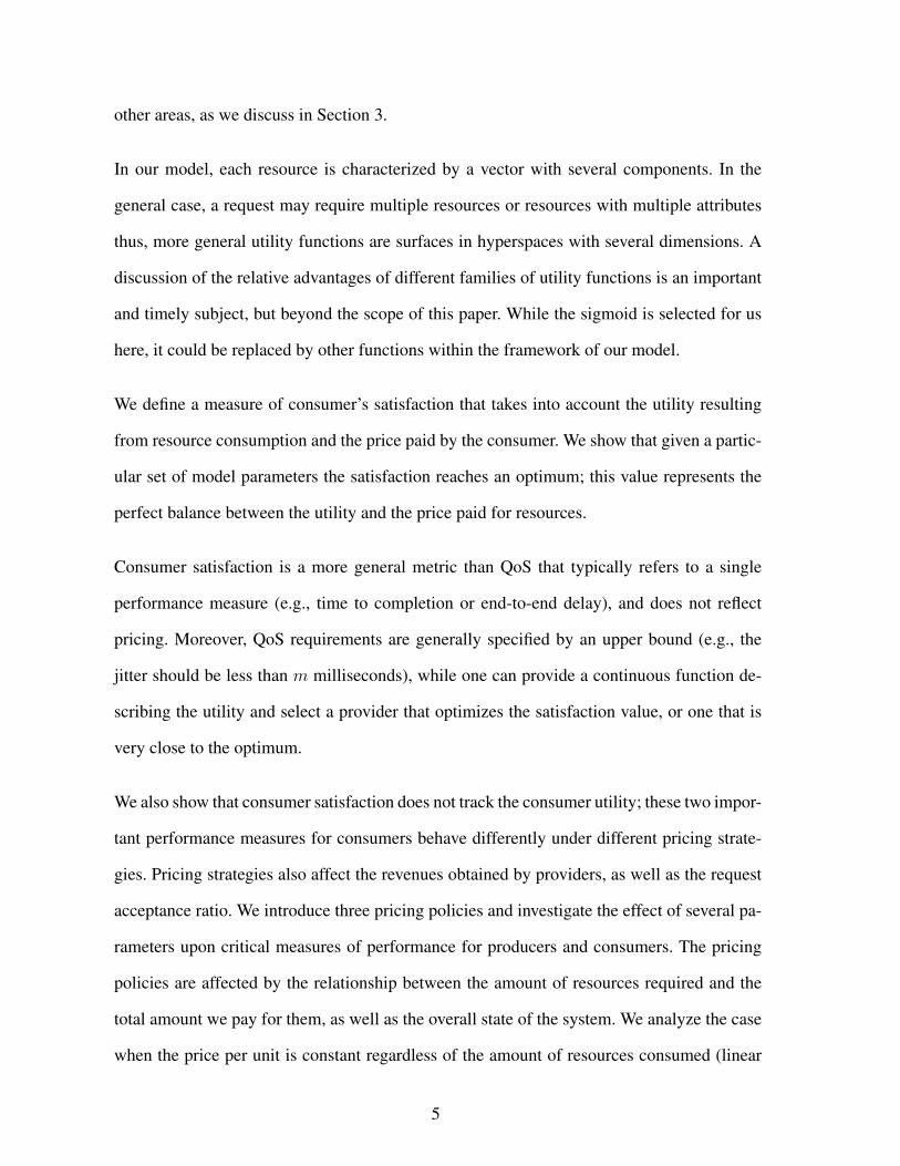
type provided by provider Rj as:

skij(u

kij, p

kij) = 1− e−κk

i ukij

µki (pk

ij/φki )−εk

i, κk

i , φki , µ

ki , ε

ki > 0

where κki , µk

i and εki are appropriate positive constants and φk

i is a reference price.

The overall satisfaction of consumer Ui for resources provided by Rj is:

• the product over the set of resources provided by Rj , i.e., sij =∏l

k=1 skij , or

• the weighted average over the set of resources provided by Rj , i.e., sij = 1l

∑lk=1 bk

ijskij ,

where bkij values are provided by consumer Ui and

∑lk=1 bk

ij = 1.

0 1000 2000 3000 40000

0.2

0.4

0.6

0.8

1

Resource: memory

Util

ity

0 1000 2000 3000 40000

0.05

0.1

0.15

0.2

Resource: memory

Pric

e

0 1000 2000 3000 40000

0.2

0.4

0.6

0.8

1

Resource: memoryS

atis

fact

ion

0 1000 2000 30000

0.2

0.4

0.6

0.8

Resource: computational power

Util

ity

0 1000 2000 30000

0.05

0.1

0.15

0.2

Resource: computational power

Pric

e

0 1000 2000 30000

0.2

0.4

0.6

0.8

1

Resource: computational power

Sat

isfa

ctio

n

Fig. 4. Example of utility (left), price (middle) and satisfaction (right) curves for two resources: mem-

ory (upper row) and computational power (lower row).

We conclude this section with an example. Let us consider a system which has two resources:

memory (measured in MBytes) and computational power (measured in MHz). Let us con-

sider a client which has its utility function calculated by setting ωm = 2000, ζm = 10 for

the memory, while for the computational power ωcp = 2000 and ζcp = 3. The shape of the

utility curve is shown in Figure 4, left. The utility curve is almost linear for the computa-

tional power, while it has a steep ramp for memory at the value of around 2000 MBytes.

A memory allocation smaller than 1000 MBytes has virtually no utility, while adding extra

memory above 3000 MBytes yields very little benefit. The price curves are shown in Fig-

20

ure 4, middle. The shapes of the curves are justified by objective considerations: for instance

high performance processors are an order of magnitude more expensive than consumer grade

processors. Finally, the satisfaction function is calculated with the values for the memory be-

ing: κm = 0.02, φm = 0.6, µm = 3 and εm = 3, while for computational power κcp = 0.03,

φcp = 0.2, µcp = 3 and εcp = 3. The satisfaction curves are shown in Figure 4, right. We

will assume that the overall satisfaction is the product of the satisfaction for memory and

computational power.

Let us now consider the case when the customer receives four offers A, B, C and D. The

offers and the associated cost and satisfaction values are summarized below:

Memory C. power Cost

memory

Cost

c. power

Total cost Satisfaction

A 3000 2000 300 60 360 0.6676

B 2500 2500 250 83.5 333.5 0.8132

C 2300 2500 230 83.5 313.5 0.7574

D 3000 2550 300 129 429 0.4338

Under these conditions, the user will choose offer B, which offers the highest satisfaction.

Notice that B is neither the offer with the largest amount of resources, neither the cheapest

offer.

4 The Role of Brokers

In this paper, we concentrate on optimal resource management policies. A policy is optimal

when the satisfaction function, which reflects both the price paid to carry out a task and the

21

utility resulting from the completion of the task, reaches a maximum. A broker attempts to

operate at or near this optimum.

The role of a broker is to mitigate access to resources. In this paper, we consider provider-

broker-consumer models that involve the set of resource providers R, the set of consumers

U , and broker B. These models assume that a consumer must get all of its resources from

a single provider. Brokers have “societal goals” and attempt to maximize the average utility

and revenue, as opposed to providers and consumers that have individualistic goals; each

provider wishes to maximize its revenue, while each consumer wishes to maximize its utility

and do so for as the lowest cost possible. To reconcile the requirements of a consumer and

the candidate providers, a broker chooses a subset of providers such that the satisfaction is

above a high threshold and all providers in the subset have equal chances to be chosen by

the consumer. We call the size of this subset satisficing size, and denote it by σ; the word

“satisfice” was coined by Nobel Prize winner Herbert Simon in 1957 to describe the desire

to achieve a minimal value of a variable instead of its maximum [34].

The resource negotiation protocol consists of the following steps:

(1) All providers reveal their capacity and pricing parameters to the broker: ∀Rj ∈ R send

vectors cj and ξj where each element corresponds to one type of resource.

(2) A consumer Ui sends to the broker a request with the following information :

(a) the parameters of its utility function: vectors ζi and ωi where each element corre-

sponds to one type of resource,

(b) the parameters of its satisfaction function: vectors µi, εi, κi and φi where each

element corresponds to one type of resource, and

(c) the number of candidate resource providers to be returned.

(3) The broker performs a brokering algorithm and returns a list of candidate resource

providers Ri to consumer Ui.

22

(4) Consumer Ui selects the first provider from Ri and verifies if the provider can allocate

the required resources. If it can not, the consumer moves to the next provider from the

list until the resources are allocated by a provider Rj .

(5) Rj notifies the broker about the resource allocation to Ui.

BROKERING ALGORITHM

INPUT request req, , , a finite set of resource providers ps

OUTPUT a finite set of suggested resource providers ss

BEGIN

determine amount so that req.u(amount) =

FOR each resource provider rp in ps

r = min (amount, available resources of rp)

satisfaction = req.s (req.u(r), rp.p(r))

END FOR

sort elements in ps according to their satisfactions

randomize the sequences of the first items in ps

keep the elements in ps that have the highest req.cardinality satisfaction degrees and remove the rest

ss = ps

END

Fig. 5. The algorithm performed by the broker. The consumer request, req, is elastic. It contains the

parameters describing u and s, the utility and satisfaction functions. τ is the target utility and σ is the

satisficing size. The cardinality specifies the number of resource providers to be returned by the

broker.

The algorithm performed by the broker is summarized in Figure 5. The amount of resources

to be allocated is determined during the algorithm according to a broker strategy. Simple

strategies would be to allocate the same amount of resources to every consumer, or to allocate

to every consumer a random amount of resources. A better strategy, used by our system,

is to allocate an amount of resources such that the utility of each type of resource to the

consumer reaches a certain target utility τ . To determine the amount of resources allocated

to the consumer, the broker uses Equation 13(a) derived from the definition of u(r), Equation

13(b):

r = e

ln( τ1−τ

)

ζ+ ln(ω)

(a) u(r) =(r/ω)ζ

1 + (r/ω)ζ (b) (13)

Several quantities characterize the resource management policy for broker B and its associ-

23

ated providers and consumers:

(a) Average hourly revenue. The average is over the set of providers connected to broker B;

the revenue of a provider is the sum of revenues from all resources it controls.

(b) Request acceptance ratio. The ratio is the number of accepted requests over the number

of requests submitted by the consumers connected to broker B. A request is accepted if a

provider able to allocate resources exists, otherwise the request is rejected and the corre-

sponding satisfaction and utility are set to 0.

(c) Average consumer satisfaction. The average is over the set of all consumers connected to

broker B.

(d) Average consumer utility. This average is over the set of consumers connected to broker

B.

In our model, a broker receives a percentage of the revenues collected by the providers con-

nected to it. More sophisticated mechanisms are possible, for example, in addition to the

percentage of the revenues collected from the providers, a broker may receive a premium

from consumers based upon their level of satisfaction. This policy would encourage brokers

to balance the interests of providers and consumers. Different brokers may have different

policies and may be required to disclose the average values for critical parameters, such as

τ and σ, and their fee structure, during the initial negotiation phase; thus, consumers and

providers will have the choice to work with a broker that best matches their own objective.

5 A Simulation Study

Market-oriented resource allocation algorithms are very difficult to analyze analytically. To

understand the behavior of the system we conducted a simulation study using YAES [9]. A

24

thorough investigation would require multiple brokers, but the model is already very complex

and would require additional protocols for broker selection and renegotiations so we are

considering the case of a single broker.

The resource allocated by provider Rj to consumer Ui are represented by a resource vector

rij = (r1ij r2

ij . . . rlij). For example, if the k-th component is secondary storage, then rk

ij =

20GB is the amount of secondary storage provided by Rj to consumer Ui. The associated

utility and satisfaction vectors are: uij = (u1ij u2

ij . . . ulij) and sij = (s1

ij s2ij . . . sl

ij). The

demand to capacity ratio for resource type k is the ratio of the amount requested by all

consumers to the total capacity of providers for resource k,∑

j ckj . The level of demand is

limited by the sigmoid shape of the utility curve and the finite financial resources of the

consumers. In the computation of the demand-capacity ratio, for each consumer and each

resource, it is assumed that for the requested rkij value the corresponding utility value uk

ij =

0.9, i.e., the consumers request an amount of rkij that results in uk

ij = 0.9. The demand to

capacity ratio vector for all resource types is η = (η1 η2 . . . ηl). For the sake of simplifying

the simulation, we only consider the case when η1 = η2 = · · · = ηl = η.

We run multiple simulation experiments for each case (50 runs/case) and compute 95% con-

fidence intervals for the results. The parameters for our experiments are:

• τ - target utility for the consumers,

• σ - satisficing size; reflects the choices given to the consumer by the broker, and

• η - demand to capacity ratio; measures the commitment and, thus, the load placed upon

providers.

We study the evolution in time of

• average hourly revenue,

• request acceptance ratio (the ratio of resource requests granted to total number of requests),

25

• average consumer satisfaction, and

• average consumer utility.

We investigate the performance of the model for different target utilities, τ , satisficing sizes,

σ, and demand to capacity ratios, η. We study several scenarios, for the linear (Equation 1),

EDN (Equation 5), and EDL (Equation 4) pricing strategies.

We simulate a system of 100 clusters and one broker. The number of nodes of each cluster is

a random variable normally distributed with the mean of 50 and the standard deviation of 30.

Each node is characterized by a resource vector containing the CPU rate, the main memory,

and the disk capacity. For example, the resource vector for a node with one 2 GHz CPU, 1

GB of memory, and a 40 GB disk is (2GHz, 1GB, 40GB).

Initially, there is no consumer in the system. Consumers arrive with an inter-arrival time

exponentially distributed with the mean of 2 seconds. The service time tij is exponentially

distributed with the mean of λ seconds. By varying the λ value we modify demand-capacity

ratio so that we can study the behavior of the system under different loads.

The request is elastic, i.e., instead of requesting a precise amount, consumers only specify

their utility and satisfaction functions. The parameters of the utility and satisfaction functions

are uniformly distributed in the intervals shown in Table 2. A request provides the parameters

of the utility function, ω and ζ , for each element of the resource vector (CPU, Memory, Disk).

We generate ω and ζ such that with a utility of 0.9, the CPU rate, memory space, and disk

space of a request are exponentially distributed with means of 2GHz, 4GB, and 80GB, and

ranges of [0.1GHz, 100GHz], [0.1GB, 200GB], and [0.1GB, 1000GB], respectively. More

precisely, for each element: (a) we generate the amount r according to the corresponding

distribution; (b) we choose a value for ω; (c) set u = 0.9 and compute the corresponding

value of ζ . For a resource vector, we let the overall utility be the product of the utilities of its

scalar resources, and the overall satisfaction be the product of the satisfaction for its scalar

26

Table 2

The parameters for the simulation are uniformly distributed. The parameters and the corresponding

intervals are shown.

Parameter CPU Memory Disk

ξ [5, 10] [5, 10] [5, 10]

ω [0.4, 0.9] [0.5, 1.5] [10, 30]

κ [0.02, 0.04] [0.02, 0.04] [0.02, 0.04]

µ [2, 4] [2, 4] [2, 4]

ε [2, 4] [2, 4] [2, 4]

φ [10, 20] [20, 40] [400, 800]

resources.

When we study the effect of the target utility τ , we use σ = 1 and η = 1.0; when we study the

effect of σ, we use τ = 0.9 and η = 1.0; and when we study the effect of η, we use τ = 0.9

and σ = 1. We also compare the system performance of our scheme for several σ values with

a random strategy. In this case, we randomly choose a provider from the set of all providers,

without considering the satisfaction function. To make the model more realistic, we allow a

resource provider to reject a consumer’s request if the available resources are insufficient to

permit both satisfaction and utility to reach 0.1.

Figures 6, 7, 8, and 9 summarize our findings. In each case, we present the three pricing

strategies, linear, EDN, and EDL. The parameters for the graphs illustrating the effect of the

target utility, τ , at the top of the figure are: σ = 1, η = 1.0, and τ = 0.8, 0.85, 0.9, and 0.95.

The graphs illustrating the effect of the satisficing size, σ, in the middle of the figure use

the following parameters: τ = 0.9, η = 1.0, and σ = 1, 10, and 20; for the random strategy,

27

σ =| R |= 50. The parameters for the graphs illustrating the effect of the demand to capacity

ratio, η, at the bottom of the figure are: τ = 0.9, σ = 1, and η = 0.5, 1.0, 1.5, and 2.0.

0 0.5 1 1.5 2

x 105

0

1

2

3

4

5x 10

6

TIME

AV

ER

AG

E H

OU

RLY

RE

VE

NU

E

τ = 0.8τ = 0.85τ = 0.9τ = 0.95

0 0.5 1 1.5 2

x 105

0

1

2

3

4

5x 10

6

TIME

AV

ER

AG

E H

OU

RLY

RE

VE

NU

E

τ = 0.8τ = 0.85τ = 0.9τ = 0.95

0 0.5 1 1.5 2

x 105

0

1

2

3

4

5x 10

6

TIME

AV

ER

AG

E H

OU

RLY

RE

VE

NU

E

τ = 0.8τ = 0.85τ = 0.9τ = 0.95

0 0.5 1 1.5 2

x 105

0

0.5

1

1.5

2x 10

7

TIME

AV

ER

AG

E H

OU

RLY

RE

VE

NU

E

σ = 1σ = 10σ = 20RANDOM

0 0.5 1 1.5 2

x 105

0

0.5

1

1.5

2x 10

7

TIME

AV

ER

AG

E H

OU

RLY

RE

VE

NU

E

σ = 1σ = 10σ = 20RANDOM

0 0.5 1 1.5 2

x 105

0

0.5

1

1.5

2x 10

7

TIME

AV

ER

AG

E H

OU

RLY

RE

VE

NU

E

σ = 1σ = 10σ = 20RANDOM

0 0.5 1 1.5 2

x 105

0

2

4

6

8

10x 10

6

TIME

AV

ER

AG

E H

OU

RLY

RE

VE

NU

E

η = 0.5η = 1.0η = 1.5η = 2.0

0 0.5 1 1.5 2

x 105

0

2

4

6

8

10x 10

6

TIME

AV

ER

AG

E H

OU

RLY

RE

VE

NU

E

η = 0.5η = 1.0η = 1.5η = 2.0

0 0.5 1 1.5 2

x 105

0

2

4

6

8

10x 10

6

TIME

AV

ER

AG

E H

OU

RLY

RE

VE

NU

E

η = 0.5η = 1.0η = 1.5η = 2.0

Fig. 6. Average hourly revenue vs. time (in seconds) for different target utilities, τ (top), satisficing

sizes, σ (middle), and demand to capacity ratios, η (bottom). The three pricing strategies are: linear

(left), EDN (center), and EDL (right).

The average hourly revenue is an important consideration for resource providers. We notice

that the three pricing strategies exhibit similar behavior: the average hourly revenue increases

rapidly during the transient period, reaches a maximum, and then converges to a steady state,

as shown in Figure 6. For the same value of the target utility, τ , the steady state value for the

linear and the EDN pricing strategies are close to one another and almost half of those for

EDL, as shown in the top row of Figure 6. In all cases, the larger τ the higher the revenue.

In these simulations, σ = 1 (the broker provides a single choice) and the demand to capacity

ratio is η = 1.0. We believe that resource fragmentation is the reason why the steady state

value is lower than the maximum attained at the end of the transient period.

28

Resource fragmentation is an undesirable phenomena where the amount of resources avail-

able cannot meet the target utility value for any request and resources remain idle. This effect

is more pronounced for larger utility values, for example for τ = 0.95 the steady state value

is some 20% lower than its corresponding maximum, while for τ = 0.8 the steady state value

is close to its corresponding maximum.

The next question is if larger satisficing size affects the average revenue. A small value of σ

limits the number of choices to consumers and this restriction leads to lower average hourly

revenues. In our experiments τ = 0.9 and η = 1.0, as shown in the middle row of Figure

6. EDN and EDL are superior to linear pricing. The larger σ, the higher the average hourly

revenue for the provider. The random strategy, which corresponds to the maximum value of

σ =| R | leads to the highest average hourly revenue.

Lastly, we see that the demand to capacity ratio also has an impact upon the average hourly

revenue that is larger for larger η for for all three pricing strategies, as shown in the bottom

row of Figure 6. The conclusion we draw from these results is that the average hourly revenue

increases when we provide a higher target utility (τ closer to 1), increase the satisficing size

(larger σ), and increase the demand to capacity ratio, η, and that differential pricing strategies

(EDN and EDL) are preferable to the linear one.

The request acceptance ratio for various pricing policies and choices of parameters is shown

in Figure 7. We find that the request acceptance ratio shows variations during the transient

period but converges to constant values in the steady state. The EDN pricing strategy appears

optimal, leading to steady state values close to 1.0 for virtually every choice of parameters,

except for the random σ. The steady state values for the linear and EDL strategies are also

high, with values larger than 0.95, but the exact amount is determined by the values of τ , η

and σ. We find that the higher the values of any of these parameters, the higher the request

acceptance ratio.

29

0 0.5 1 1.5 2

x 105

0.93

0.94

0.95

0.96

0.97

0.98

0.99

1

TIME

RE

QU

ES

T A

CC

EP

TA

NC

E R

AT

IO

τ = 0.8τ = 0.85τ = 0.9τ = 0.95

0 0.5 1 1.5 2

x 105

0.995

0.996

0.997

0.998

0.999

1

TIME

RE

QU

ES

T A

CC

EP

TA

NC

E R

AT

IO

τ = 0.8τ = 0.85τ = 0.9τ = 0.95

0 0.5 1 1.5 2

x 105

0.93

0.94

0.95

0.96

0.97

0.98

0.99

1

TIME

RE

QU

ES

T A

CC

EP

TA

NC

E R

AT

IO

τ = 0.8τ = 0.85τ = 0.9τ = 0.95

0 0.5 1 1.5 2

x 105

0.973

0.9735

0.974

0.9745

0.975

0.9755

0.976

TIME

RE

QU

ES

T A

CC

EP

TA

NC

E R

AT

IO

σ = 1σ = 10σ = 20RANDOM

0 0.5 1 1.5 2

x 105

0.93

0.94

0.95

0.96

0.97

0.98

0.99

1

TIME

RE

QU

ES

T A

CC

EP

TA

NC

E R

AT

IO

σ = 1σ = 10σ = 20RANDOM

0 0.5 1 1.5 2

x 105

0.93

0.94

0.95

0.96

0.97

0.98

0.99

1

TIME

RE

QU

ES

T A

CC

EP

TA

NC

E R

AT

IO

σ = 1σ = 10σ = 20RANDOM

0 0.5 1 1.5 2

x 105

0.972

0.973

0.974

0.975

0.976

0.977

TIME

RE

QU

ES

T A

CC

EP

TA

NC

E R

AT

IO

η = 0.5η = 1.0η = 1.5η = 2.0

0 0.5 1 1.5 2

x 105

0.93

0.94

0.95

0.96

0.97

0.98

0.99

1

TIME

RE

QU

ES

T A

CC

EP

TA

NC

E R

AT

IO

η = 0.5η = 1.0η = 1.5η = 2.0

0 0.5 1 1.5 2

x 105

0.93

0.94

0.95

0.96

0.97

0.98

0.99

1

TIME

RE

QU

ES

T A

CC

EP

TA

NC

E R

AT

IO

η = 0.5η = 1.0η = 1.5η = 2.0

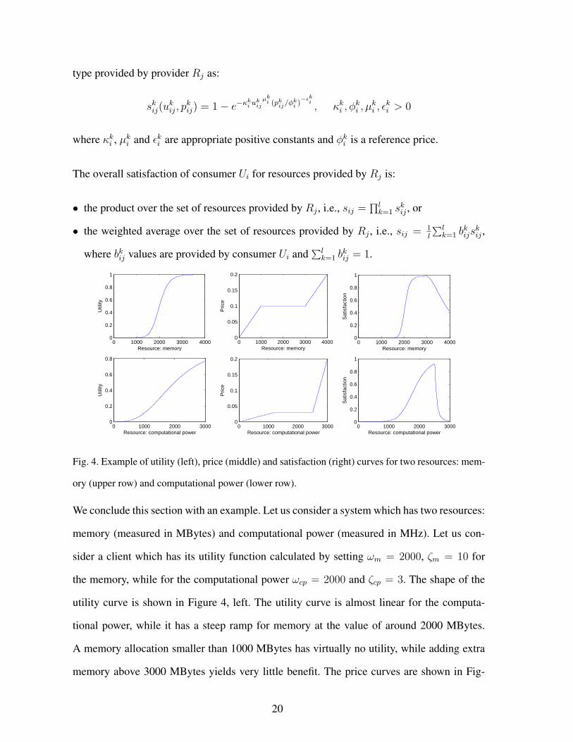
Fig. 7. Request acceptance ratio vs. time (in seconds) for different target utilities, τ (top), satisficing

sizes, σ (middle), and demand to capacity ratios, η (bottom). The three pricing strategies are: linear

(left), EDN (center), and EDL (right).

The three pricing strategies lead to very different consumer satisfaction for the same set of

parameters of the simulation, even though the qualitative behavior is somehow similar in that

the average consumer satisfaction decreases during the transient period and then increases

and reaches a stable value in steady state, as shown in Figure 8. EDN appears to be best

strategy. The larger the target utility, the lower the consumer satisfaction. The highest steady

state average satisfaction is about 80% when τ = 0.8 and when we use the EDN strategy

as compared with less than 50% for EDL and about 70% for linear pricing strategy in terms

of σ. The highest satisfaction occurs when σ = 1. Though this seems counterintuitive it is

well justified; in this case the broker directs the consumer to that resource provider that best

matches the request. When we select at random one provider from the list of all providers

supplied by the broker we observe the lowest average consumer satisfaction because we

30

0 0.5 1 1.5 2

x 105

0.2

0.4

0.6

0.8

1

1.2

TIME

AV

ER

AG

E C

ON

SU

ME

R S

AT

ISF

AC

TIO

N

τ = 0.8τ = 0.85τ = 0.9τ = 0.95

0 0.5 1 1.5 2

x 105

0.2

0.4

0.6

0.8

1

1.2

TIME

AV

ER

AG

E C

ON

SU

ME

R S

AT

ISF

AC

TIO

N

τ = 0.8τ = 0.85τ = 0.9τ = 0.95

0 0.5 1 1.5 2

x 105

0.2

0.4

0.6

0.8

1

1.2

TIME

AV

ER

AG

E C

ON

SU

ME

R S

AT

ISF

AC

TIO

N

τ = 0.8τ = 0.85τ = 0.9τ = 0.95

0 0.5 1 1.5 2

x 105

0.2

0.4

0.6

0.8

1

1.2

TIME

AV

ER

AG

E C

ON

SU

ME

R S

AT

ISF

AC

TIO

N

σ = 1σ = 10σ = 20RANDOM

0 0.5 1 1.5 2

x 105

0.2

0.4

0.6

0.8

1

1.2

TIME

AV

ER

AG

E C

ON

SU

ME

R S

AT

ISF

AC

TIO

N

σ = 1σ = 10σ = 20RANDOM

0 0.5 1 1.5 2

x 105

0.2

0.4

0.6

0.8

1

1.2

TIME

AV

ER

AG

E C

ON

SU

ME

R S

AT

ISF

AC

TIO

N

σ = 1σ = 10σ = 20RANDOM

0 0.5 1 1.5 2

x 105

0.2

0.4

0.6

0.8

1

1.2

TIME

AV

ER

AG

E C

ON

SU

ME

R S

AT

ISF

AC

TIO

N

η = 0.5η = 1.0η = 1.5η = 2.0

0 0.5 1 1.5 2

x 105

0.2

0.4

0.6

0.8

1

1.2

TIME

AV

ER

AG

E C

ON

SU

ME

R S

AT

ISF

AC

TIO

N

η = 0.5η = 1.0η = 1.5η = 2.0

0 0.5 1 1.5 2

x 105

0.2

0.4

0.6

0.8

1

1.2

TIME

AV

ER

AG

E C

ON

SU

ME

R S

AT

ISF

AC

TIO

N

η = 0.5η = 1.0η = 1.5η = 2.0

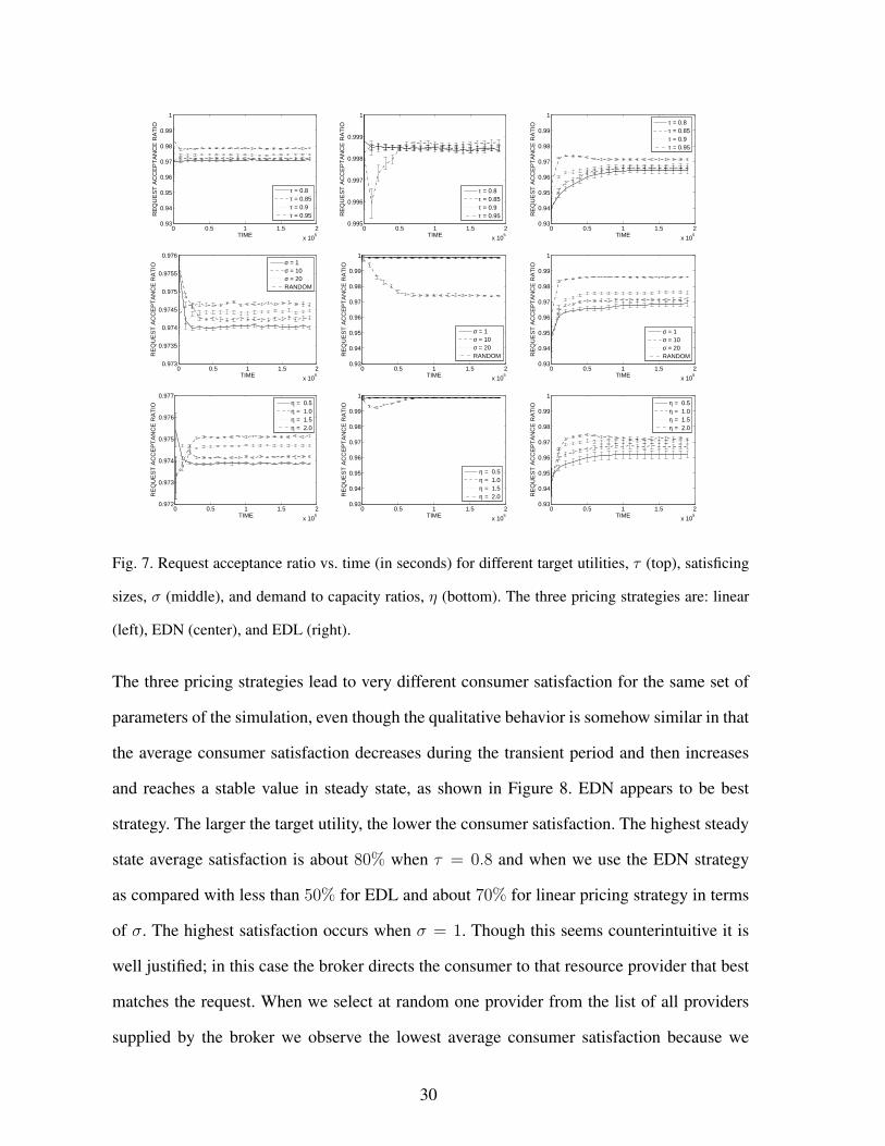
Fig. 8. Average consumer satisfaction vs. time (in seconds) for different target utilities, τ (top), sat-

isficing sizes, σ (middle), and demand to capacity ratio, η (bottom). The three pricing strategies are:

linear (left), EDN (center), and EDL (right).

have a high probability to select a less than optimal match for a given request. Recall that the

optimal match is the top ranked element of the list of providers supplied by the broker. We

also notice that a high demand to capacity ratio has a negative impact upon user satisfaction.

The largest impact of the demand to capacity ratio upon the steady state average consumer

satisfaction is visible for the linear pricing strategy, when the average consumer satisfaction

ranges from about 55% for η = 2.0 to about 75% for η = 0.5.

For the same set of parameters of the simulation the three pricing strategies lead to slightly

different average consumer utility values, but the qualitative behavior is similar, as shown in

Figure 9. The average consumer utility decreases slowly during the transient period because

of system fragmentation; some resources are allocated to consumers due to their cheaper

price, although they are not enough to allow the utility to reach the target value, τ . In steady

31

0 0.5 1 1.5 2

x 105

0.3

0.4

0.5

0.6

0.7

0.8

0.9

1

TIME

AV

ER

AG

E C

ON

SU

ME

R U

TIL

ITY τ = 0.8

τ = 0.85τ = 0.9τ = 0.95

0 0.5 1 1.5 2

x 105

0.3

0.4

0.5

0.6

0.7

0.8

0.9

1

TIME

AV

ER

AG

E C

ON

SU

ME

R U

TIL

ITY τ = 0.8

τ = 0.85τ = 0.9τ = 0.95

0 0.5 1 1.5 2

x 105

0.3

0.4

0.5

0.6

0.7

0.8

0.9

1

TIME

AV

ER

AG

E C

ON

SU

ME

R U

TIL

ITY τ = 0.8

τ = 0.85τ = 0.9τ = 0.95

0 0.5 1 1.5 2

x 105

0.3

0.4

0.5

0.6

0.7

0.8

0.9

1

TIME

AV

ER

AG

E C

ON

SU

ME

R U

TIL

ITY

σ = 1σ = 10σ = 20RANDOM

0 0.5 1 1.5 2

x 105

0.3

0.4

0.5

0.6

0.7

0.8

0.9

1

TIME

AV

ER

AG

E C

ON

SU

ME

R U

TIL

ITY

σ = 1σ = 10σ = 20RANDOM

0 0.5 1 1.5 2

x 105

0.3

0.4

0.5

0.6

0.7

0.8

0.9

1

TIME

AV

ER

AG

E C

ON

SU

ME

R U

TIL

ITY

σ = 1σ = 10σ = 20RANDOM

0 0.5 1 1.5 2

x 105

0.3

0.4

0.5

0.6

0.7

0.8

0.9

1

TIME

AV

ER

AG

E C

ON

SU

ME

R U

TIL

ITY η = 0.5

η = 1.0η = 1.5η = 2.0

0 0.5 1 1.5 2

x 105

0.3

0.4

0.5

0.6

0.7

0.8

0.9

1

TIME

AV

ER

AG

E C

ON

SU

ME

R U

TIL

ITY η = 0.5

η = 1.0η = 1.5η = 2.0

0 0.5 1 1.5 2

x 105

0.3

0.4

0.5

0.6

0.7

0.8

0.9

1

TIME

AV

ER

AG

E C

ON

SU

ME

R U

TIL

ITY η = 0.5

η = 1.0η = 1.5η = 2.0

Fig. 9. Average consumer utility vs. time (in seconds) for different target utilities, τ (top), satisficing

sizes, σ (middle), and demand to capacity ratios, η (bottom). The three pricing strategies: linear (left),

EDN (center), and EDL (right).

state, the average utility reaches a stable value. Overall, the differentiated pricing strategies,

EDN and EDL, perform better and reach higher steady state values. The higher the target

utility, the larger the actual utility; the highest steady-sate utility is about 70% for τ = 0.95

for EDN and EDL, as shown in the top of Figure 9. The larger the satisficing size, the higher

the actual utility; the random strategy leads to 90% utility, as shown in the middle of Figure

9. The lower the demand to capacity ratio, the higher the satisfaction.

Figure 10 summarizes the effect of the three pricing strategies upon the four quantities we

monitored in our experiments, for a particular set of parameters: τ = 0.9, σ = 1, and η = 1.0.

EDL allows the highest average hourly revenue while the linear pricing strategy leads to the

lowest one, as shown in Figure 10(a). EDN leads to the highest request acceptance ratio while

EDL leads to the lowest one, as shown in Figure 10(b). EDN leads to the highest consumer

32

0 0.5 1 1.5 2

x 105

0

0.5

1

1.5

2

2.5

3

3.5x 10

6

TIME

AV

ER

AG

E H

OU

RLY

RE

VE

NU

E

LINEAREDNEDL

0 0.5 1 1.5 2

x 105

0.94

0.95

0.96

0.97

0.98

0.99

1

TIME

RE

QU

ES

T A

CC

EP

TA

NC

E R

AT

IO

LINEAREDNEDL

(a) (b)

0 0.5 1 1.5 2

x 105

0.3

0.4

0.5

0.6

0.7

0.8

0.9

1

TIME

AV

ER

AG

E C

ON

SU

ME

R S

AT

ISF

AC

TIO

N

LINEAREDNEDL

0 0.5 1 1.5 2

x 105

0.55

0.6

0.65

0.7

0.75

0.8

0.85

0.9

0.95

TIME

AV

ER

AG

E C

ON

SU

ME

R U

TIL

ITY LINEAR

EDNEDL

(c) (d)

Fig. 10. (a) The average hourly revenue, (b) the request acceptance ratio, (c) the average consumer

satisfaction, and (d) the average consumer utility vs. time (in seconds) for σ = 1, τ = 0.9, and

η = 1.0, with different price functions.

satisfaction while EDL leads to the lowest one, as shown in Figure 10(c). EDL allows the

highest average hourly revenue while linear pricing strategy leads to the lowest one, as shown

in Figure 10(d).

6 Conclusions and Future Work

Economic models are notoriously difficult to study. The complexity of the utility, price, and

satisfaction-based models precludes analytical studies and in this paper we report on a sim-

33

ulation study. The goal of our simulation study is to validate our choice of utility, price,

and satisfaction function, to study the effect of the many parameters that characterize our

model, and to get some intuition regarding the transient and the steady-state behavior of our

models. We are primarily interested in qualitative rather than quantitative results, i.e., we are

interested in trends, rather than actual numbers.

In our model the actual shape of the utility function is controlled by the parameters dictated

primarily by the application. On the other hand, the satisfaction function reflects mostly the

user’s constraints. The model inhibits selfish behavior: greedy consumers pay a hefty price

and greedy providers who insist on high prices are avoided. The satisfaction function ensures

a balance between the amount of resources consumed and the price paid for them.

The function of a broker is to monitor the system and set τ and σ for optimal performance.

For example, if the broker perceives that the average consumer utility is too low, it has two

choices: increase τ or increase σ. At the same time, the system experiences an increase of

the average hourly revenue and a decrease of the average consumer satisfaction. The fact

that increasing utility could result in lower satisfaction seems counterintuitive, but reflects

the consequences of allocating more resources; we increase the total cost possibly beyond

the optimum predicated by the satisfaction function. The simulation results shown in this

paper are consistent with those in [5,6] where we use linear pricing and simpler models

based upon a synthetic quantity to represent a vector of resources.

The EDL pricing strategy leads to the highest average consumer utility and the highest aver-

age hourly revenue, while it gives the lowest request acceptance ratio and the lowest average

consumer satisfaction. The EDN pricing strategy allows the highest request acceptance ra-

tio and the highest average consumer satisfaction, while it leads to lower average consumer

utility and average hourly revenue than EDL. It is also remarkable that the average consumer

satisfaction does not track the average consumer utility. This shows the importance of the

34

satisfaction function.

One could argue that in practice it would be rather difficult for users to specify the parameters

of their utility and satisfaction function. Of course, this is true in today’s environments, but

entirely feasible in intelligent environments where such information could be provided by

societal services [7]. The advantages of elastic requests is likely to motivate the creation of

such services in the computational economy of the future.

Even though we limit our analysis to a single broker system, we are confident that the most

important conclusions we are able to draw from our model, namely that:

(i) Given a particular set of model parameters the satisfaction reaches an optimum; this value

represents the perfect balance between the utility and the price paid for resources,

(ii) The satisfaction does not track the utility,

(iii) Differentiated pricing perform better than linear pricing,

(iv) Brokers can effectively control the computing economy

will still be valid for multiple broker systems. In such an environment, individual brokers

could enforce different policies; providers and consumers could join the one that best matches

their individual goals. The other simplifying assumptions for our analysis, e.g., the unifor-

mity of the demand to capacity ratio for all resources available at a consumer’s site, will

most likely have second order effects. The restriction we impose by requiring a consumer to

obtain all necessary resources from a single broker is also unlikely to significantly affect our

findings.

It is very difficult to make a direct comparison between systems based on different mod-

els with different objective functions. Our results are qualitative rather than quantitative; the

goal of our work is to show that our formal mathematical model captures and predicts per-

35

formance trends. In Table 1 we compare the features of several systems. Performance results

for existing systems are rarely reported and when they are available it would be hard to cali-

brate them. We are confident that a model that formalizes the selfish goals of consumers and

providers, as well as societal goals, has a significant potential. Our intention is to draw the

attention of the community to the potential of utility, price, and satisfaction-based resource

allocation models. It is well beyond the scope of this paper to cover all angles of such a

complex model.

A fair number of questions require further investigations including: (a) Are there better alter-

natives to the utility, price, and satisfaction functions we introduced? (b) Is the policy aiming

to achieve maximum satisfaction sound, e.g., how should we take into account the societal

importance of activities carried out by individual resource consumers? (c) How can we apply

the models to more complex networks of resource managers? (d) What composition rules

should be used to describe the utility and/or the satisfaction for a group of consumers? (e)

How can we define more complex utility functions that take into account additional con-

straints related to system reliability and deadlines? Future work involves also the study of

more complex systems including policy makers and multiple brokers.

7 Acknowledgments

This research was supported in part by National Science Foundation grants ACI-0296035,

EIA-0296179, and CNS-0615170, the Colorado State University George T. Abell Endow-

ment, and the DARPA Information Exploitation Office under contract No. NBCHC030137.

The authors are greatly indebted to three anonymous reviewers for their constructive com-

ments which helped improve the quality of this paper. One of the authors (dcm) acknowl-

edges useful discussions regarding the Kelly model with Don Towsley. Preliminary versions

and performance results presented in this paper were reported in [5,6].

36

References

[1] Y. Amir, B. Awerbuch, A. Barak, R. S. Borgstrom, and A. Keren. An opportunity cost approach

for job assignment in a scalable computing cluster. IEEE Trans. on Parallel and Distributed

Systems, 11(7):760–768, 2000.

[2] Y. Amir, B. A. B, and R.S.Borgstrom. A cost-benefit framework for online management of a

metacomputing system. In Proc. 1st Int. Conf. on Information and Computation Economies

(ICE 98), pp. 14–47. ACM Press: New York, 1998.

[3] A. Anastasiadi, S. Kapidakis, C. Nikolaou, and J. Sairamesh. A computational economy

for dynamic load balancing and data replication. In Proc 1st Int. Conf. on Information and

Computation Economics ICE’98, 1998.

[4] L. Badia and M. Zorzi. On utility-based radio resource management with and without service

guarantees. In Proc. ACM MSWiM 2004, Modelling, Analysis, and Simulation of Wireless and

Mobile Systems, pp. 244–251. ACM Press, 2004.

[5] X. Bai, L. Boloni, D. C. Marinescu, H. J. Siegel, R. A. Daley, and I.-J. Wang. Are utility, price,

and satisfaction based resource allocation models suitable for large-scale distributed systems? In

Proc. 3rd Int. Workshop on Grid Economics and Business Models (GECON 2006) , Singapore,

2006.

[6] X. Bai, L. Boloni, D. C. Marinescu, H. J. Siegel, R. A. Daley, and I.-J. Wang. A brokering

framework for large-scale heterogeneous systems. 15th Heterogeneous Computing Workshop

(HCW 2006) in Proc. 20th IEEE Int. Parallel and Distributed Processing Symp. (IPDPS 2006)

(CD Proceedings), Rhodes, 2006.

[7] X. Bai, H. Yu, G. Wang, Y. Ji, G. M. Marinescu, D. C. Marinescu, and L. Boloni. Coordination

in intelligent grid environments. Proc. of the IEEE, 93(3):613–630, 2005.

[8] M. Blaugh. Economic Theory in Retrospect. Cambridge University Press, 5th Edition, ISBN

978-0521577014, 1997

37

[9] L. Boloni and D. Turgut. YAES - a modular simulator for mobile networks. In Proc. 8-th

ACM/IEEE Int. Symp. on Modeling, Analysis and Simulation of Wireless and Mobile Systems

MSWIM 2005, pp. 169–173, 2005.

[10] R. Buyya, D. Abramson, and J. Giddy. Nimrod/g: An architecture of a resource management and

scheduling system in a global computational grid. In Proc. 4 th Int. Conf. on High Performance

Computing in the Asia Pacific Region, 1:283–289, 2001.

[11] R. Buyya, H. Stockinger, J. Giddy, and D. Abramson. Economic models for management

of resources in peer-to-peer and grid computing. In Proc. SPIE Int. Conf. on Commercial

Applications for High-Performance Computing, pp. 13–25, Denver, 2001.

[12] B. Chun and D. Culler. Market-based proportional resource sharing for clusters. Technical report,

UC Berkeley, Sept. 1999.

[13] CONDOR. URL http://www.cs.wisc.edu/condor/.

[14] B. F. Cooper and H. Garcia-Molina. Peer-to-peer data preservation through storage auctions.

IEEE Trans. Parallel Distrib. Syst., 16(3):246–257, 2005.

[15] ContractNet FIPA standard URL http://www.fipa.org/specs/fipa00029/

[16] R. Frisch. Propagation problems and impulse problems in dynamc economics. In Econnomic

Essays in Honour of Gustav Cassel, pp. 691-704, Allen and Unwin, London, 1933. Reprinted in

“Readings in Business Cycles,” R. A. Gordon and L. R. Klein, Eds., 1966.

[17] P. Ghosh, N. Roy, S. K. Das, and K. Basu. A pricing strategy for job allocation in mobile

grids using a non-cooperative bargaining theory framework. J. Parallel Distrib. Comput.,

65(11):1366–1383, 2005.

[18] J. Gomoluch and M. Schroeder. Market-based resource allocation for grid computing: A model

and simulation. In Int. Middleware Conf., Workshop Proc., pp. 211–218, Rio de Janeiro, 2003.

[19] C. Grothoff. Resource allocation in peer-to-peer networks - an excess-based economic model.

Wirtschaftsinformatik, 45(3):285–292, 2003.

38

[20] L. He and T. R. Ioerger. Task-oriented computational economic-based distributed resource

allocation mechanisms for computational grids. In Proc. Int. Conf. on Artificial Intelligence,

volume 1, pp. 462–468, Las Vegas, 2004.

[21] G. Heiser, F. Lam, and S. Russel. Resource management in the Mungi single-address-space

operating system. In Proc. 21 st Australasian Computer Science Conf., pp. 417–428, 1998.

[22] HP Grid computing. URL http://www.hp.com/techservers/grid.

[23] IBM Grid computing. URL http://www.ibm.com/grid.

[24] S. U. Khan and I. Ahmad. Non-cooperative, semi-cooperative, and cooperative games-based grid

resource allocation. Proc. Int. Parallel & Distrib. Proc. Symp, (IPDPS 2006), 2006.

[25] F. Kelly. Models for a self-managed Internet. Philosophical Transactions of the Royal Society,

A358:2335–2348, 2000.

[26] S. Lalis and A. Karipidis. Jaws: An open market-based framework for distributed computing

over the internet. In R. Buyya and M. Baker, Eds., GRID, volume 1971 of LNCS, Springer, pp.

36–46. 2000.

[27] Mariposa. URL http://mariposa.cs.berkeley.edu/.

[28] L. W. McKnight and J. Boroumand. Pricing Internet services: Approaches and challenges. IEEE

Computer, 33(2):128–129, 2000.

[29] N. Nisan, S. London, O. Regev, and N. Camiel. Globally distributed computation over the

internet - the popcorn project. In ICDCS ’98: Proc. 18th Int. Conf. on Distributed Computing

Systems, pp. 592–601, Washington, 1998. IEEE Computer Society.

[30] Nobel Lectures, Economics 1969-1980, From Nobel Lectures, Economics 1969-1980, A.

Lindbeck, Editor, World Scientific Publishing, Singapore, 1992.

[31] D. Reed, I. Pratt, P. Menage, S. Early, and N. Stratford. Xenoservers: Accountable execution of

untrusted programs. In Workshop on Hot Topics in Operating Systems, pp. 136–141, 1999.

39

[32] SETI@home. URL http://setiathome.ssl.berkeley.edu/.

[33] W. Shen, Y. Li, H. H. Genniwa, and C. Wang. Adaptive negotiation for agent-based grid

computing. Journal of the American Statistical Association, 97(457), 2002.

[34] H. A. Simon. Models of Man. Wiley, 1957.

[35] R. G. Smith. The contract net protocol: high-level communication and control in a distributed

problem solver. IEEE Trans. on Computers Vol C-29, 12:1104 – 1113, 1980.

[36] B. Snowdown, H. R. Vane. Modern Macroeconomic: Tts Origin, Development and Current

Status. Edward Elgar Publishing, New Edition, ISBN 978-1845422080, 2005.

[37] M. Stonebraker, R. Devine, M. Kornacker, W. Litwin, A. Pfeffer, A. Sah, and C. Staelin. An

economic paradigm for query processing and data migration in Mariposa. In Proc. 3rd Int. Conf.

on Parallel and Distributed Information Systems, 1994.

[38] Sun Microsystems utility computing. URL http://www.sun.com/service/utility.

[39] H. R. Varian. Intermediate Microeconomics: A Modern Approach. Norton, New York, 1999.

[40] W. Vickrey. Counterspeculation and competitive sealed tenders. Journal of Finance, 16(1):8–37,

1961.

[41] C. A. Waldspurger, T. Hogg, B. A. Huberman, J. O. Kephart, and W. S. Stornetta. Spawn: A

distributed computational economy. Software Engineering, 18(2):103–117, 1992.

[42] R. Wolski, J. S. Plank, J. Brevik, and T. Bryan. Analyzing market-based resource allocation

strategies for the computational Grid. The Int. Journal of High Performance Computing

Applications, 15(3):258–281, 2001.

[43] R. Wolski, J. S. Plank, J. Brevik, and T. Bryan. G-commerce: Market formulations controlling

resource allocation on the computational grid. In Proc. 15th Int. Parallel & Distributed

Processing Symposium (IPDPS-01), pp. 23–27, San Francisco, CA, April 2001.

40