A Look on the Cost Side: Market Share and the Competitive Environment

INFORMS is collaborating with JSTOR to digitize, preserve and extend access to Marketing Science.

http://www.jstor.org

A Look on the Cost Side: Market Share and the Competitive Environment Author(s): William Boulding and Richard Staelin Source: Marketing Science, Vol. 12, No. 2 (Spring, 1993), pp. 144-166Published by: INFORMSStable URL: http://www.jstor.org/stable/184037Accessed: 20-03-2015 14:38 UTC

Your use of the JSTOR archive indicates your acceptance of the Terms & Conditions of Use, available at http://www.jstor.org/page/info/about/policies/terms.jsp

JSTOR is a not-for-profit service that helps scholars, researchers, and students discover, use, and build upon a wide range of contentin a trusted digital archive. We use information technology and tools to increase productivity and facilitate new forms of scholarship.For more information about JSTOR, please contact [email protected].

This content downloaded from 152.3.153.137 on Fri, 20 Mar 2015 14:38:46 UTCAll use subject to JSTOR Terms and Conditions

http://www.jstor.org

http://www.jstor.org/action/showPublisher?publisherCode=informs

http://www.jstor.org/stable/184037

http://www.jstor.org/page/info/about/policies/terms.jsp


MARKETING SCIENCE Vol. 12, No. 2, Spring 1993

Printed in U.S.A.

A LOOK ON THE COST SIDE: MARKET SHARE AND THE COMPETITIVE ENVIRONMENT

WILLIAM BOULDING AND RICHARD STAELIN Duke University

In this paper we develop a model relating market share to average costs. We start with a theoretical model of the factors that affect the firm's average cost curve, partitioning these factors into (a) measurable firm and competitive environment characteristics, and (b) unobserved factors that are either fixed, random, or follow a first-order autoregressive process. We then link this theoretical model to an empirical model in which we specify three average cost equations for the organizational areas of purchasing, production, and marketing. Main effects for initial (lagged) market share position, as well as their interactions with factors characterizing the firm's competitive environment, represent the variables of key theoretical interest in our equations. We estimate these equations using PIMS data, and control for fixed, contemporaneous, and autoregressive unobservable factors. Our results suggest that market share can often lead to market power in the form of lower average costs. However, the firm's operating environment greatly moderates the effect of market share on average cost. In particular, we find that market share position only leads to lower average costs when the organizational unit operates in a competitive environment that

gives it both motivation and ability to realize power from its market share position. (Market Share; Average Costs; Market Power; Organizational Complacency; PIMS Data; Panel Data Estimation; Competitive Strategy; Econometric Models)

1. Introduction

The relationship between market share and firm performance has been of considerable interest to researchers and business strategists for several decades. At least three schools of thought exist on the nature of this relationship. One view holds that the nature of this relationship is causal, and emerges from the structure-performance paradigm (Bain 1951 ). Specifically, it holds that market share causes higher prices and lower costs, thus yielding greater profitability. In the marketing area the work of Buzzell et al. (1975) is most

typically identified with this view. A different view is espoused in the work by Demsetz (1973, 1974). This view suggests reverse causality between share and performance; that is, greater efficiency leads to lower costs, which then leads to greater market share. Yet a third view acknowledges a strong correlation between market share and performance, but attributes this to skill, luck, or other unobserved stochastic factors (Mancke 1974, Rumelt and Wensley 1980, Lippman and Rumelt 1982, Jacobson and Aaker 1985, Boulding and Staelin 1990). In this paper we test the proposition that increases in market share lead to lower costs while controlling for the latter two explanations.

Much of the conflicting empirical evidence in the literature can be attributed to meth-

odological issues associated with analyzing existing data bases. For example, factors specific 144

0732-2399/93/1202/0144$01.25 Copyright ? 1993, The Institute of Management Sciences/Operations Research Society of America



MARKET SHARE AND THE COMPETITIVE ENVIRONMENT

to a firm such as managerial skill and the economies of manufacturing scale often are not measured, yet these factors are believed to affect both the variable of strategic interest (e.g., market share), and the dependent variable (e.g., firm performance). Omitting these factors results in biased estimates. Also, due to data limitations, many of the available empirical models represent reduced form estimates of proposed strategy models. As an example, although the hypothesized effects of market share typically operate through prices and costs, most cross-firm market share models employ ROI, not prices and/or costs, as the dependent variable. One suspects that this choice results not from a desire for parsimony, but rather because of the unavailability of usable price and cost data for a cross-section of firms.

Probably the most heavily utilized data source for empirical strategy research is PIMS (see Buzzell and Gale 1987 for a bibliography). Despite its extensively discussed limitations (e.g., Anderson and Paine 1978), recent methodological advances utilizing the panel nature of the PIMS data show that many of the limitations are perceived, rather than actual. For example, work by Jacobson (1990) and Boulding (1990) discusses solutions to the problem of bias caused by unobservables in business performance models. Other work enables access to previously unusable disguised dollar amount variables by solving the disguise bias problem (Moore and Boulding 1987, Hagerty et al. 1988). Work by Boulding and Staelin (1990) expands on the technique demonstrated by Moore and Boulding (1987), using accounting identities to derive usable measures of average price and average cost when performing analyses across firms. In combination, these papers greatly enhance the value of the PIMS data base for strategic research by enabling one to control for factors missing from the PIMS data, as well as adding average cost and price to the set of variables available for strategic analysis.

This paper draws on the above noted advances and uses the PIMS database to gain new insights into the market share-firm performance relationship. In particular, we focus on the cost side of market share-firm performance relationship. The cost of this restricted focus is that it does not indicate the overall effect of market share on firm performance, as is provided by a summary measure such as ROI. However, the benefit of this focus on cost side effects is a better understanding of the underlying process by which market share influences a major determinant of firm performance.

Our basic approach is to partition the effects of market share on the cost structure of a firm into two components. The first effect is associated with the volume resulting from the firm obtaining a particular share of industry sales. Specifically, we ask the question, do larger volumes associate with lower average costs? The second effect is associated with the market share position of the firm after adjusting for volume. The question here is, does market share position, independent of the volume associated with this market share, provide high share firms an opportunity to extract cost concessions in its interactions with outside agents, thereby resulting in lower average costs? We expand on this latter question by addressing the issue of whether this market share effect is conditional on the nature of the firm's competitive environment.

In performing our analyses we look at three components of cost, i.e., (1) inbound (purchasing) costs, (2) processing (production) costs, and (3) outbound (marketing) costs. Thus, our analysis continues the trend of recent empirical studies by obtaining estimates of the effects of market share on different aspects of firm performance (Farris et al. 1989, Boulding and Staelin 1990). As a result, a clearer picture emerges concerning the overall organizational effects due to the strategic choice of market share.

We develop the paper as follows. First, based on a set of concepts grounded in economics, organization theory, and behavioral theory, we posit four basic principles. These four principles form the basis for our hypotheses as to when and how the two components of market share affect the cost structure of a firm. We then build a theoretical model that allows tests of these hypotheses. Next, we review the data constraints of our sample and

145



WILLIAM BOULDING AND RICHARD STAELIN

develop our empirical model. Section 5 presents the estimation results, and ?6 discusses strategic implications.

2. Hypotheses

Our interest centers on how market share influences the average cost of a firm, with the fundamental research question being when, if ever, market share position has any economic value above and beyond its volume influence on average cost. In order to address this question we start with four fundamental principles that generate all of our hypothesized effects. We first state these four principles, and then discuss the concepts that underlie them in greater detail:

(1) A firm operates on an average cost curve that is either monotonically decreasing, monotonically increasing, or U-shaped.

(2) A firm's ability to lower its average costs is increased by either a good market share position or by an easy competitive environment, or both.

(3) A firm's motivation to lower its average costs is increased by either internal pressure (self-imposed) or external pressure (imposed by competition), or both.

(4) For a firm to realize benefits in the form of lower average costs, it must possess both the ability and motivation to decrease costs.

Our first principle requires little discussion. It simply reflects that one should be flexible in representing the relationship between a specific firm's average costs and volume. For example, while firms may initially garner economies of scale, one might expect marginal costs to ultimately exceed average costs, thus leading to increasing average costs. In any event, changes in volume reflect movement along this average cost curve, and could result in either increases or decreases in average cost depending on the firm's position on the curve.

Our second principle is concerned with conditions that could potentially lead to a shift in the average cost curve, as opposed to movement along the average cost curve. However, it should be noted that ability to lower costs is not synonymous with realization of lower costs. Thus, market share (or an easy competitive environment) does not in itself cause lower costs.

More specifically, based upon the substantial and still growing, albeit controversial, literature in economics (e.g., Martin 1988, Schroeter 1988, Staten et al. 1988), we posit that higher market share increases a firm's ability to lower average costs. Implicit in this share-power premise, is that high market share allows firms to gain either price (monopoly power) or cost (monopsony power) benefits, relative to low market share firms, in their relationships with suppliers, channel members, and buyers. Thus, firm power could man- ifest itself in the form of obtaining lower input costs from suppliers; obtaining more functions from channel members at a given price; providing buyers with lower quality (i.e., cheaper) products or services which are nevertheless purchased at the same price; or expending less effort marketing these products or services.

Our belief that an easier competitive environment increases the firm's ability to get lower average cost also derives from economic theory. The logic behind this belief is that easy environments reduce competition, thus keeping input and output costs lower at the margin.

Principle three addresses the motivation of the organization to obtain lower average costs. We base this principle in part on the premise found in the behavioral theory of the firm (Cyert and March 1963), which has firms scanning the environment as part of the planning process. This environmental scanning yields information on what we label "external pressure." We posit that easy competitive environments (i.e., low external pressure), result in what the behavioral theory of the firm labels "organizational slack." We refer to this slack as the firm having less motivation to reduce costs.

Easy competitive environments are not the only cause of organizational slack in our

146



https://www.researchgate.net/publication/24094642_Market_Power_andor_Efficiency?el=1_x_8&enrichId=rgreq-9ae90af0-1f7c-42bd-860e-37d04c1a9ac4&enrichSource=Y292ZXJQYWdlOzIyNzQ0MjAzODtBUzoyMDkwOTA0MjU5NTQzMDRAMTQyNjg2MjQ1MDE3MA==

https://www.researchgate.net/publication/24094610_Estimating_the_Degree_of_Market_Power_in_the_Beef_Packing_Industry?el=1_x_8&enrichId=rgreq-9ae90af0-1f7c-42bd-860e-37d04c1a9ac4&enrichSource=Y292ZXJQYWdlOzIyNzQ0MjAzODtBUzoyMDkwOTA0MjU5NTQzMDRAMTQyNjg2MjQ1MDE3MA==


formulation. Slack also occurs when the organization becomes successful. One frequently hears the phrase "fat and happy" to describe this situation. More formally, the behavioral theory of the firm describes this phenomenon, which we label "internal pressure," as the firm's aspiration level. We posit that a measure of organizational success/aspiration level is market share. We state this belief independent of whether or not market share causes profits. Instead, we rely on the evidence that market share strongly correlates with profitability (Buzzell et al. 1975). This association leads us to posit that as market share reaches/surpasses the firm's aspiration level, motivation to reduce costs due to internal pressure decreases. Alternatively, one can simply state that success breeds complacency, as discussed in organizational behavior textbooks (e.g., Mainiero and Tromley 1989).

Principle four derives from the standard ability-motivation paradigm frequently utilized in behavioral research. This paradigm, which originates from Heider ( 1958), posits that performance requires both ability (which Heider refers to as "can") and motivation (which Heider refers to as "trying").

It should be noted that market share and the competitive environment affect both the ability and motivation constructs. However, these two factors influence ability and motivation in opposite directions. Thus, as market share increases, or the competitiveness of the environment decreases, ability to lower costs increases, but motivation to reduce costs decreases. As a result, the effects of market share or competitive environment on costs appear ambiguous, at first glance. However, when one considers the interaction of these factors one can begin to make unambiguous predictions. For example, consider a scenario in which a firm has a good market share position in a difficult competitive environment. In this scenario ability is "on," due to a good market share position, and motivation is "on," due to external pressure from a hostile competitive environment. Therefore, the firm benefits in the form of obtaining lower average costs.

Table 1 presents four combinations of market share position and competitive environment, where each factor can be either "good" or "bad." It delineates the effects of these individual factors on ability and motivation, as well as the predicted effect of the combination of these factors on cost benefits accruing to the firm. A key point to be drawn from this table is that we do not view a firm's ability and motivation levels as formed in a compensatory fashion. If this were the case, high motivation from a difficult environment would be moderated, and ultimately canceled out by low motivation from a high market share position. Rather, we consider ability and motivation levels as generated in a disjunctive fashion, such that either, but not necessarily both, market share or competitive environment can trigger motivation and ability. We reflect this logic in Table 1 by including a heading for the "overall impact" of market share and competitive environment on motivation and ability.

To summarize our Table 1 predictions, a firm with a bad market share position in a bad competitive environment receives no cost reduction benefits, since they have no ability to obtain lower costs. A firm with a good market share position in a good competitive environment also receives no cost reduction benefits, since they have no motivation to obtain lower costs. However, in a bad competitive environment with a good market share position, and vice-versa, the firm obtains lower average costs since it has both ability and motivation to reduce costs.

Table 1 thus yields a series of testable predictions, all of which are conditional, on the effects of market share and competitive environment. More formally, we state hypotheses relating to deviations from the base condition of bad market share position and a bad competitive environment. Note that these hypotheses relate to shifts in the average cost curve.

In order to test for these shifts, we must first control for movement along the average cost curve. Our first hypothesis bears on the shape of the average cost curve, and derives directly from our first principle. As such, the hypothesis is not very restrictive:

147




TABLE 1

Predicted Marker Share/Competitive Environment Effects

Impact on Impact on Condition Motivation Ability Predicted Effect

(1) Bad Market Share + Bad Competitive Environment +

Overall Impact: + -No Cost Benefits

(2) Good Market Share - + Bad Competitive Environment +

Overall Impact: + + Cost Benefits

(3) Bad Market Share + Good Competitive Environment - +

Overall Impact: + + Cost Benefits

(4) Good Market Share - + Good Competitive Environment - +

Overall Impact: -+ No Cost Benefits

H1: All else equal, firms operate in a region of the average cost curve that is either monotonically increasing, monotonically decreasing, or U-shaped.

Our next three hypotheses relate to shifts in the average cost curve, after controlling for movement along the average cost curve. These hypotheses derive from principles two

through four, as summarized in Table 1, with the usual ceteris paribus caveats, and relate to the conditional effects of market share position and the competitive environment:

H2: Holding fixed a bad competitive environment, increasing levels of market share cause decreasing levels of average costs.

H3: Holding fixed a bad market share position, increasingly good competitive environments lead to decreasing levels of average costs.

H4: Simultaneous improvements in both market share position and the competitive environment ultimately lead to no motivation to reduce costs, and thus yield dissipating cost benefits.

In stating these hypotheses, notice we do not specify differential effects for the three cost areas of the firm. However, Table 2, which describes the characteristics of the three cost areas, indicates differences between these areas. In particular, purchasing and mar-

keting cost outcomes are typically negotiated with outside agents, whereas production

TABLE 2

Cost Component Characteristics

Characteristic Purchasing Production Marketing

Area Managers' Cost Minimize costs in all Minimize unit costs Minimize unit costs Orientation: transactions subject subject to

to downstream downstream demands demands

External Agents: Suppliers Labor Distribution Channels

Ad Agencies Buyers

Determination of Cost Negotiated Internally determined Negotiated Outcome:

148




costs are typically internally determined, with the exception of labor costs. Since the market share position effect operates via the firm interacting with outside agents one might argue that market share position provides no ability to reduce production costs. (Although production does interact with outside labor agents, labor market competition is typically independent of factor or product market competition.) Alternatively, one might argue that market share provides indirect, or "passed through," ability to reduce production costs via interaction with outside agents in the purchasing and marketing areas (e.g., the purchasing area negotiates for more timely delivery of raw materials for production; or the marketing area negotiates for less timely delivery of finished products to customers). Which of these conjectures holds depends on the extent to which orga- nizations have coordinated internal relationships (Deming 1986). Thus, we leave the resolution of these opposing conjectures as an empirical question.

3. Theoretical Model Development

The preceding discussion outlines our beliefs on how volume and market share position, conditional on the competitive environment, affect the three components of average cost. In order to test these beliefs we develop structural equations for a firm's average cost by department, and then develop a methodology for estimating the parameters of theoretical interest in the equations.

We start with the nonrestrictive assumption that firms face an average cost curve, and location on this curve is determined by the firm's chosen output level. Next, we acknowledge that a firm's average cost can change for a multitude of reasons other than market share position, and that these reasons either can result in movement along the average cost curve (e.g., a demand shift) or a shift in the average cost curve. We control for the former by making average cost a function of endogenously determined quantity, and the latter by including both internal firm actions and external forces as independent variables in the average cost function.

We test our hypotheses by performing a within-across firm analysis. We pool across firms because the number of data points available for any one firm in our database precludes meaningful analysis with respect to our hypotheses. However, use of cross- sectional data requires us to adjust for factors that differ across firms. Consequently, we take into consideration not only factors that vary within firms and affect demand or average costs, e.g., shifts in consumer tastes, changes in product quality, changes in the competitive environment, etc., but also factors that vary across firms, e.g., firm size, managerial expertise, efficiency, etc.

We formalize the preceding discussion by making the following assumptions: ( 1 ) Increases in quantity can result in either increases or decreases in average cost.

The downward portion of this curve can be captured by Q'1, where Q denotes quantity sold, and y, < 0. The upward-sloping portion of this curve can be represented by Q-l+DY2, where D is a dummy indicator which assumes a value of 1 when marginal costs exceed average costs (in which case the average cost curve is upward sloping), zero otherwise, and 72 + 7'I > 0.

(2) Shifts in firm i's average cost curve during period t are caused by a vector of firm characteristics and actions (F1i), and competitive environment factors (Z,t), where both vectors can be measured, and increasing values of Z represent increasingly good competitive environments. These shifts can be represented by exp(ilFit) and exp(t2Zit) respectively, where /31, 02, Fit, and Zit are vectors.

(3) Another set of shifts are caused by factors that are unobservable. Assume these unobservable factors can be partitioned into three categories, those which are (a) fixed over the period of analysis, (b) random, or (c) follow a first-order autoregressive process. Specifically let ai represent the fixed effect, pti the random component, and P/it-i the first-order autogressive process, where 6i-I =-- it- + POit-2-

149




(4) Shifts in firm i's average cost curve can be caused by the firm's prior dollar market share position ($MSit_,). Moreover, the magnitude of these effects can vary according to the competitive environment. These shifts are represented by exp(P3$MSit,-), and exp( 34$MSitl * Zit), respectively, where P4 is a vector.

These assumptions lead to the following equation for departmental average cost (ACit), where we suppress department subscripts for parsimony:

ACil = Q1,+Dit2 exp(i Fi, + 32Zi, + 3$MSit-1 + 4$MSi-l *Zi + ai a+ iu + Ppeit- ). ( 1 )

This formulation allows testing of our stated hypotheses. The y coefficients on quantity allow us to test HI. More specifically, Y1 represents the downward sloping portion of the

average cost curve, and (,y + 72) represents the upward sloping portion of this relationship. Thus, HI suggests that 7 is less than zero and 72 is greater than the absolute value of y .

With respect to our other hypotheses, notice that condition ( 1 ) from Table 1 represents the base case in this model, since under our scaling bad market share position and bad competitive environment are both denoted by zero. Condition (2) in Table 1 corresponds to H2, and represents the deviation from the base condition resulting from increasing levels of market share. Thus, we can test H2 in this model by determining if the main effect of market share position, i.e., the coefficient /3, yields a statistically significant negative sign. Condition (3) from Table 1 corresponds to H3, and represents the deviation from the base condition resulting from increasingly good competitive environments. Consequently, we can test H3 by seeing if the /2 coefficients on the competitive environment variables demonstrate the expected negative signs. Finally, H4 corresponds to condition (4) from Table 1. Since simultaneously improving market share position and competitive environment reduces motivation (and thus cost benefits), this effect will reduce the positive benefits suggested by conditions (2) and (3). Therefore, we can test

H4 by checking the /4 coefficients on the market share-competitive environment interaction terms for their expected positive sign.

To prevent bias in our coefficients of theoretical interest, and thus cleanly test our stated hypotheses, we must control for the unobserved factors a,, 4,'t, and PEit-,. In the

next section we present such an approach. In addition, we describe how we operationalize the measures for each of the above-mentioned variables.

4. Data and Model Estimation

As noted previously, we use PIMS data to estimate our model, a database both much used and much criticized (e.g., see Anderson and Paine 1978, Ramanujam and Ven- katraman 1984). The promise contained in the PIMS data is the diverse sample, and the detailed description of the company, competitive environment, and customer base, and thus the ability to discern generalizable strategic relationships (e.g., see Buzzell and Gale 1987). However, this diversity causes difficulties when an analysis treats all business units as "equal" on dimensions not measured by the PIMS data.

In order to fulfill the promise inherent in PIMS data, while avoiding some of the difficulties, we exploit the panel nature of the data. Our sample consists of a time-series cross-section (i.e., the SPIYR database) of all business units for which PIMS has at least four years of history (these data span the years 1970 to 1987); where a business unit is defined as a division of a firm selling a distinct set of products to an identifiable set of customers, in competition with a well-defined set of competitors (Strategic Planning Institute 1987). Our sample contains annual data for 1,736 different business units. Before transformations, we have 13,764 observations for these business units. This sample ultimately reduces to 2,555 observations for our estimating equations after controlling for unobserved variables.

150




Dependent Variables

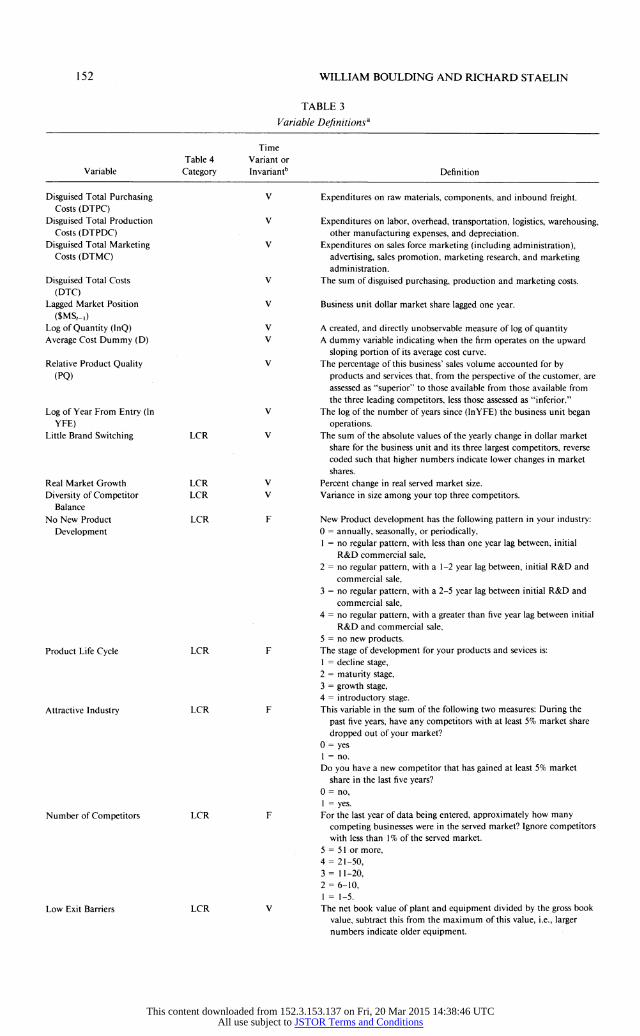
PIMS reports information about costs in separate categories for purchasing, production, and marketing. Purchasing costs consist of raw material and component costs, as well as inbound freight. Production costs consist of labor, including overhead, transportation, logistics and warehousing, manufacturing, and depreciation expenses. Marketing costs include salesforce expenses, advertising and sales promotion, marketing administration, and marketing research. We report these, and all other variable definitions in Table 3. We also note that these variables may not reflect "true" costs, as is often the case with accounting data. For example, we do not directly measure cost of capital (the discount rate times the asset base). Rather, we can only proxy this cost of capital measure via depreciation. To the extent that depreciation rates deviate from the true cost of capital, this introduces error into our manufacturing and total average cost variables, thereby increasing the amount of noise in our empirical modeling.

Two other limitations exist with the cost variables as measured and reported in PIMS. First, each business unit disguises its cost data by multiplying all dollar measures by its own time-invariant disguise factor Ki. Second, data are reported in the form of total, rather than average, costs. We show below, using techniques originally developed by Moore and Boulding (1987) and Boulding and Staelin (1990), how we obtain usable measures of average costs for estimation purposes. However, the particular derivations are unique to this paper.1 In order to conserve space we show this for only one dependent measure, average purchasing costs (APC), although we derive the other two average cost measures in an identical fashion.

Ignoring firm subscripts for simplicity, we begin with the accounting identities

APC- TPC/Q-= TPCt/(TR,/Pt), (2)

where APCt = average unit purchasing costs for year t, TPCt = total purchasing costs, Qt = quantity in units, TR, = total revenues, and Pt = firm's price. PIMS does not contain direct measures of any of the variables included in the accounting identities. However, we observe disguised total purchasing costs (DTPCt) and disguised total revenues (DTRt), which we can write as DTPCt TPCt * Ki, and DTRt = TR, * Ki, where Ki represents the business unit-specific, time-invariant disguise factor.

Using the information from above, we can rewrite (2) multiplying both numerator and denominator by Ki, resulting in

APC - Ki*TPCt/(Ki *TR,/P,). (3)

Since DTPCt K, *TPCt, and DTRt- K, *TRt, we could derive average costs using disguised measures from the PIMS data if we observed Pt. However, Pt is not measured in the PIMS data. Consequently, we must remove Pt from our analysis. We do this by first writing equation (3) in terms of time t - 1, which yields

APCt-_ = Ki*TPCt-1/(Ki *TRt_-/P,t_). (4)

Taking logs and subtracting (4) from (3) yields

In APCt - In APCt- In DTPCt - In DTPCt- - In DTRt + In DTR,-l + In Pt- In P,_-. (5)

Note that the PIMS data contain measures on everything on the right-hand side in (5) except for the price variables, which still appear. However, PIMS does contain a price

' In fact, we believe that the derivation of average cost in this paper is superior to the method used in Boulding and Staelin (1990), since it is completely based on internal firm information. The Boulding and Staelin (1990) method relies on a mix of internal measures and competitive measures (e.g., relative price). The internal measures should contain less error relative to external (competitive) measures, which causes us to prefer the method utilized in this paper.

151




TABLE 3

Variable Definitionsa

Time Table 4 Variant or

Variable Category Invariantb Definition

Disguised Total Purchasing Costs (DTPC)

Disguised Total Production Costs (DTPDC)

Disguised Total Marketing Costs (DTMC)

Disguised Total Costs (DTC)

Lagged Market Position ($MS,_,)

Log of Quantity (InQ) Average Cost Dummy (D)

Relative Product Quality (PQ)

Log of Year From Entry (In YFE)

Little Brand Switching

Real Market Growth Diversity of Competitor

Balance No New Product

Development

Product Life Cycle

Attractive Industry

Number of Competitors

Low Exit Barriers

LCR

LCR LCR

LCR

LCR

LCR

LCR

LCR

V Expenditures on raw materials, components, and inbound freight.

V Expenditures on labor, overhead, transportation, logistics, warehousing, other manufacturing expenses, and depreciation.

V Expenditures on sales force marketing (including administration), advertising, sales promotion, marketing research, and marketing administration.

V The sum of disguised purchasing, production and marketing costs.

V Business unit dollar market share lagged one year.

V A created, and directly unobservable measure of log of quantity V A dummy variable indicating when the firm operates on the upward

sloping portion of its average cost curve. V The percentage of this business' sales volume accounted for by

products and services that, from the perspective of the customer, are assessed as "superior" to those available from those available from the three leading competitors, less those assessed as "inferior."

V The log of the number of years since (InYFE) the business unit began operations.

V The sum of the absolute values of the yearly change in dollar market share for the business unit and its three largest competitors, reverse coded such that higher numbers indicate lower changes in market shares.

V Percent change in real served market size. V Variance in size among your top three competitors.

F New Product development has the following pattern in your industry: 0 = annually, seasonally, or periodically, I = no regular pattern, with less than one year lag between, initial

R&D commercial sale, 2 = no regular pattern, with a 1-2 year lag between, initial R&D and

commercial sale, 3 = no regular pattern, with a 2-5 year lag between initial R&D and

commercial sale, 4 = no regular pattern, with a greater than five year lag between initial

R&D and commercial sale, 5 = no new products.

F The stage of development for your products and sevices is: I = decline stage, 2 = maturity stage, 3 = growth stage, 4 = introductory stage.

F This variable in the sum of the following two measures: During the

past five years, have any competitors with at least 5% market share dropped out of your market?

0 = yes 1 = no.

Do you have a new competitor that has gained at least 5% market share in the last five years?

0 = no, 1 = yes.

F For the last year of data being entered, approximately how many competing businesses were in the served market? Ignore competitors with less than 1% of the served market.

5 = 51 or more, 4 = 21-50, 3 = 11-20, 2 = 6-10, 1 = 1-5.

V The net book value of plant and equipment divided by the gross book value, subtract this from the maximum of this value, i.e., larger numbers indicate older equipment.

152




TABLE 3 (continued)

Time Table 4 Variant or

Variable Category Invariantb Definition

Patent Protection BTE F Does your business benefit from patents on product or process? 0 = no, I = on either product or process, 2 = on both product and process.

Shared Costs BTE F This variable is the sum of the shared facilities, markets/distribution channels, and marketing programs, where shared facilities are coded:

I = less than 10% of P&E, 2 = between 10% and 80% of P&E, 3 = 80% or more of P&E, shared markets/distribution channels are coded: I = less than 25% of sales, 2 = 25% to 49% of sales, 3 = 50% to 74% of sales, 4 = 75% or more of sales, and shared marketing programs are coded: I = less than 10% of marketing, 2 = between 10% and 80% of marketing, 3 = 80% or more of marketing.

Disguised Replacement BTE V The log of the plant and equipment replacement value for the business Value unit.

Disguised R&D BTE V The log of total annual R&D expenditures for the business unit.

Expenditures Disguised Working Capital BTE V The log of total annual working capital requirement for the business

unit.

Preemptive Capacity BTE V The business unit's standard capacity divided by the size of the served market.

a Many of these variables have been recoded from their original values. Definition comes from the PIMS codebook (Strategic Planning Institute

1988) and data forms (Strategic Planning Institute 1987). b Time variant = V, time invariant = F (fixed).

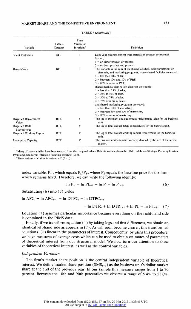
index variable, PI,, which equals Pt/PB, where PB equals the baseline price for the firm, which remains fixed. Therefore, we can write the following identity:

In P, - In PI,1 = In P, - In P,_1. (6)

Substituting (6) into (5) yields

In APC - In APC,- = In DTPC - In DTPC,-i

- In DTR, + In DTR,_- + In PI, - In PI,_-. (7)

Equation (7) assumes particular importance because everything on the right-hand side is contained in the PIMS data.

Finally, if we transform equation (1) by taking logs and first differences, we obtain an identical left-hand side as appears in (7). As will soon become clearer, this transformed equation ( 1 ) is linear in the parameters of interest. Consequently, by using this procedure, we have measures of average costs which can be used to obtain estimates of parameters of theoretical interest from our structural model. We now turn our attention to these variables of theoretical interest, as well as the control variables.

Independent Variables

The firm's market share position is the central independent variable of theoretical interest. We define market share position ($MSt_1) as the business unit's dollar market share at the end of the previous year. In our sample this measure ranges from 1 to 70 percent. Between the 10th and 90th percentiles we observe a range of 5.4% to 53.0%,

153




and a median of 20.7%. As frequently noted about PIMS member companies (e.g., see Day 1986), most of the units within our sample have a relatively strong market share position. However, substantial variation exists, thereby allowing us to test our market position hypotheses.

Quantity is another variable of theoretical interest that is not directly available in the PIMS database. As noted above, in order to derive estimable average cost variables we take logs and first differences of equation ( 1 ). Thus, for estimating purposes we need to obtain the measure In Qt - In Qt-1, where Qt is the firm's output over period t. We do this by starting with the accounting identity

Qt-TRt/Pt or, (8)

KiQl DTRt/Pt, (9)

where all the variables are as previously defined. As before, write (9) for time t - 1, resulting in

KiQt --DTRt-I/Pt-1. (10)

Take logs on (9) and (10), subtract (10) from 9), and write P in terms of PI using equation (6), yielding

In Qt - In Qt-1 In DTRt - In DTRt_i - In PIt + In PIt_-. (11)

Since both DTR and PI are available in the PIMS database, this yields a usable measure of quantity for estimating our empirical model.

We also include a dummy variable D interacted with a quantity term to capture the upward sloping portion of the average cost curve. Since we estimate three different cost equations we actually create three of these dummy variables. However, to conserve space we illustrate how we create this variable for the purchasing costs equation. Specifically, define the following dummy variable:

D l if MPCit/APCit > 1,

Dit = 0 otherwise.

In the above notation MPC refers to the marginal purchasing costs. Thus, our dummy variable reflects the mathematical fact that if marginal costs are greater than average costs, then the average cost curve must be upward sloping. Although neither MPCit or

APCi, is individually observable in the PIMS data, it can be shown that the ratio MPCi,/ APCit is observable.2

We should note that we consider quantity endogenously determined by the firm. This

endogeneity implies that our structural model includes a quantity equation. However, since we have no theoretical interest in the quantity equation, we present only reduced form results. As will soon become clearer, we use only appropriately lagged variables as instruments to avoid problems of contemporaneous correlation.

Our model also includes measures of the competitive environment. These matter for control purposes, since they may directly affect the average cost curve, and because we believe the competitive environment moderates market share effects. We choose to characterize the competitive environment by using two of the forces of competition from the

2 In particular, the following expression reduces to

MPCi,/APCi,: [(DTPCi, - DTPC,- )/( DTRi,/PIi, - DTRi,-i/PIi,- )]/[DTPCi,/(DTRi,/PIi,)],

where all terms in this expression are as previously defined. As noted by a reviewer, this may confuse a total and partial derivative, i.e., confuse dynamic shifts in the average cost curve with movement along a static average cost curve. Consequently, this ratio may be measured with error.

154




framework originally proposed by Porter (1980). This framework represents one possible approach for representing industry structure/competitiveness. We refer to these two external forces as the lack of existing competitive rivalry (LCR) within the industry and the barriers to entry (BTE), the latter representing potential competitive rivalry. Note that we do not include measures for buyer power or supplier power, since we are attempting to measure whether market share provides power over buyers (monopoly power) or power over suppliers (monopsony power) in terms of obtaining lower costs.

Using Porter (1980) as a guide, we select individual variables found in the PIMS data that measure different aspects of the current and potential competitive forces. Table 4 reports the variables used to create our two measures of the competitive environment. Specific definitions for each component making up the forces are found in Table 3.

We note that the PIMS data provide imperfect proxies for our underlying constructs of current and potential competitive rivalry. For example, within an industry one would certainly expect an industry with new entrants, and thus an increased number of competitors, to become more rivalrous than before the new entries. However, our LCR measure assumes that new entry and higher numbers of competitors indicate less competitive rivalry. The reason for this apparent inconsistency is that the entry and number of competitors information in PIMS does not change over time. Therefore, this information only reflects cross-sectional, versus within-industry, differences. Furthermore, it is possible that on a cross-sectional basis, industries with less competitive rivalry attract new entries and higher numbers of competitors. Said differently, the issue is whether these variables measure a change in the competitive environment, or a signal of the competitive conditions. As an empirical check on our conjecture that these variables represent signals of attractive conditions, we decompose the competitive rivalry construct and find that the entry/no exits and number of competitors variables produce the same directional effects as the rest of the components. This empirical result gives credence to the cross-sectional, versus within-industry, interpretation of these variables.

In addition, we note that our measure of lack of competitive rivalry may simplify complex/conditional relationships. For example, we measure the lack of brand switching (i.e., product differentiation) in terms of stability of market shares. We acknowledge that this measure may have different implications for competitive rivalry in early growth versus mature/declining industries. To the extent these simplifications increase error in our competitive rivalry measures, we should observe a decrease in our ability to detect effects of these constructs in our empirical modeling.

Given these caveats as to the imperfect nature of our measures, we operationalize our measures of LCR and BTE as follows. First, take the variables found under the subheadings in Table 4, standardize them with mean zero, and then sum the standardized factors. Next, rescale the resulting variables to strictly nonnegative values. This means that a value of "0" for our two aggregated measures of the competitive environment represents the base case in our model (e.g., the worst possible competitive environment encountered in our sample), while increasing values represent increasingly good competitive environments. For this reason we label our constructs lack of competitive rivalry and barriers to entry.

Our model also includes two time-varying firm specific variables for control purposes. First, we include a measure of product quality (PQ), because the firm's choice of quality can potentially shift its average cost curve.3 Second, we include a proxy variable for firm

3 There is good reason to consider the PIMS measure of quality as endogenously determined in firm performance models (e.g., see Jacobson and Aaker 1987). Therefore, we test for the endogeneity of product quality, but fail to reject the hypothesis of exogenously determined product quality in any of our models (tl,2531

= 0.73, 0.63, 0.50, and 0.35 for purchasing, manufacturing, marketing, and total average costs, respectively). Therefore, we treat product quality as exogenous in estimation.

155




TABLE 4

Factors that Characterize the Firm's Competitive Environment

Lack of Competitive Rivalry (LCR)

Industry has little brand switching Industry has high real-market growth Industry has variance in size of competitors Industry has no regular new product introductions Product is early in product life cycle Industry has recent entrant and/or no recent exits Industry has many competitors Firms have low exist costs

Barriers to Entry (BTE)

BU has patent protection BU has high shared costs BU has high capital costs:

High replacement value of plant and equipment High R&D expenditures High working capital requirements

BU preempts capacity for its served market

experience. Specifically, we include the log of the number of years from the firm's initial entry (In YFE) to control for learning curve differences between firms.

Our theoretical model also includes unspecified firm-specific time-invariant effects (ai), serially correlated effects (pEit-i), and random events (iti). We specify this error structure because many unobserved factors, such as firm efficiency, skill, scale, dissipating returns to an earlier investment, luck, etc., potentially influence both the demand curve and average cost curve facing the individual business. Although we do not measure these variables, we explicitly allow for their existence in our structural model, and subsequently show how we control for these omitted factors by removing their effects from the estimating equations. This prevents the coefficients on our variables of theoretical interest from containing bias due to unobservable fixed, first-order autoregressive, and random variables. We next describe the estimation procedure that enables us to control for these three sets of unobserved factors.

Estimation

To linearize our model and remove unobserved fixed effects requires log and first difference transformations of our structural model. Specifically, taking logs of equation ( 1) produces

In ACi, = y, In Qi, + Di,y2 In Qi, + 13 Fit + 2Zit

+ f3$MSit-i + -4$MSit- *Zit + ai + Ei-. (12)

Lagging (12) one period, subtracting this expression from (12), and recognizing that eit = Ait + P-it-l, yields

In AC, - In ACi-,I = y1 (ln Qi, - In Qit-l) + Y2(Dit*ln Qit - Dit,_*ln Qit-1)

+ 1 (Fi, -

Fit-) + f2(Zit -

Zit-i) + -3($MSit,- -

$MSi-2)

156




+ 34($MSitI *Zit - $MSit-2*Zit-l) + lit

-(1 - P)(Pei-2 + Hit-), (13)

thereby removing ai. Since the error structure for equation (13) still contains an autoregressive component, we lag (13) one period, multiply this lagged equation by the autoregressive parameter p, and then subtract the resulting equation from (13), yielding

In ACi, - In ACi,- - p(ln ACit- - In ACit-2)

= 71((ln Qit - In Qi-i) - p(ln Qit-1 - In Qit-2))

+ y2((Di,*ln Qi, - Dit,-*ln Qit- ) - p(Di-I*ln Qi,-i - Dit-2*1n Qit-2))

+ ,1((Fi, - Fitl) - p(Fit- - Fit-2)) + f2((Zit - Zit-)- (Zit- - Zit-2))

+ /3(($MSit- - $MSit-2)- p($MSit-2- $MSit-3))

+ /44(($MSit_ * Zit - $MSit-2 * Zit) - I p($MSit-2 * Zit- -$MSit_3 * Zit-2))

+ t - -1. (14)

Although taking first differences and then p-differencing controls for unobserved fixed effects and first-order autoregressive effects, this procedure does not sufficiently solve all of the potential unobserved variable problems. Specifically, as empirically shown by Jacobson and Aaker (1985) and Rumelt and Wensley (1980), another unobservability problem plagues market share-firm performance models. To see this, assume there exists a randomly occurring unobserved variable, such as luck, that contemporaneously affects both the firm's demand curve and its market share. Since shifts in demand for the profit maximizing firm result in movement along its average cost curve, failure to control for this movement leads one to mistakenly attribute these changes in average cost to market share position rather than the randomly occurring event. More specifically, failure to control for unobserved demand shifts that drive actual market share might result in an inability to discriminate between two hypotheses for a relationship between market share and average costs: (a) a firm chooses a new point on the same average cost curve due to a demand shift, or (b) the firm incurs a shift in its average cost curve.

We circumvent this problem by using a 2SLS estimation procedure in which we instrument our market share variables as they appear on the right-hand side of our model. Following Jacobson (1990), we use lagged values as instruments; in our case we use two period lags since our estimating equation contains both At and At-i in the error term.4 In this way, as urged by Lippman and Rumelt (1982), we control for contemporaneous unobserved stochastic factors that affect both average costs and market shares.5

In summary, equation (14) represents our estimating equation for each of the three cost components. Note eight important characteristics about equation (14). First, estimation of this equation yields estimates on the structural parameters of theoretical interest from equation (1), i.e., 'Y, 'Y2, il, 102, /33, and /4. Second, we can substitute in our

4 Since the error structure in the estimating equation contains random error from years t and t - 1, any variables we consider endogenous and appear in our estimating equation for either years t or t - 1 (i.e., the market share and quantity variables) must be instrumented to ensure independence from the remaining error term.

5 Our treatment of market share as endogenous implies that our structural model also includes a market share equation. Since we have no theoretical interest in a structural market share equation, we present only reduced form results. Thus, we do not explore the question of whether lower average costs cause higher market shares (although we control for this possibility in exploring whether the reverse is true). However, importantly, the results for the average cost equations are exactly the same as if we did simultaneously estimate and report a market share equation.

157




derived average cost measure in equation (7) for the dependent variable in equation ( 14). Third, we can substitute into equation (14) our derived measure for quantity from equation (1 1 ).6 Fourth, the differencing transformation eliminates the firm-specific time- invariant component, ai, from the estimating equation. Thus, although we do not estimate ai, we control for the possibility that fixed, firm-specific unobservables such as managerial efficiency, firm size, and industry, might affect average costs. In this way our analysis builds on the work in the area of cost and production function estimation dating back to Hoch (1955) and Mundlak ( 1961 ), which suggests the use of within group estimators to control for unobserved managerial efficiency. Fifth, the p-differencing procedure eliminates the autoregressive error from our data. Consequently, equation (14) controls for unobserved variables that follow a first-order autoregressive process. Such variables could include managerial efficiency and consumer tastes. Sixth, since p is not known, we must search over all possible values of p to determine its value.7 Seventh, we need to eliminate any possible correlation between the market share position and quantity variables and the remaining contemporaneous error, tt - _t1. We do this by treating market share and quantity as endogenous in our two-stage least squares estimation procedure, in which we utilize variables lagged two and three periods as instruments. Eighth, although the error structure contains only white noise, adjacent observations from the same firm will be correlated since the white noise contains random error from two consecutive years. Consequently, to guarantee consistent estimates of the standard errors we drop every other observation from the analysis.8

Finally, we adjust the nominal dollar amounts for our cost variables into constant dollars via use of the GNP deflator. In addition, we include time dummies to capture any misspecification of the deflator or any omitted time-specific information. We do not discuss these time dummies further, as they serve a control purpose, but have no strategic implications.

5. Results

Table 5 presents results from our estimation of equation (14) for the three different cost areas. All reported results employ the value of p that minimizes the sums of squared errors. The maximum likelihood estimate of p for the purchasing costs equation equals 0.20, for production costs 0.05, and for marketing costs 0.00. Using these consistent estimates of p in estimation of equation (14) allows us to simultaneously test all stated hypotheses without fear of bias due to first-order autoregressive error. We frame our discussion of results around these hypotheses, and then turn to findings with respect to control variables of interest.

6 Since we only observe quantity in its differenced form, this means we cannot multiply our dummy variable

Di, times the annual value of quantity sold, but instead must multiply the dummy by the difference in quantity sold. In other words, we must assume that firms operate on the same half of the U-shaped curve in consecutive

years. This implies that we measure our structural variable Dit*ln Qit, (in log form) with error. Thus, our estimates of -y and Y2 will be downward biased, making tests of significance for these coefficients more conservative.

7 Note that the expression p(ln ACit_, - In ACit-2) in equation (14) can be moved to the right-hand side. This makes clear that estimates of p may be biased since the term (In ACit_1 - In ACit-2) will not be independent of the random error in equation (14). Therefore, in order to obtain consistent estimates of p, we instrument the term (In ACi-l - In ACi,-2) using instruments lagged two and three periods in order to guarantee independence from the random error term. We thank Bob Jacobson for bringing this to our attention.

8 Another analysis approach which uses all available data (thus increasing efficiency in estimation), directly accounts for the interfirm error covariance structure. An Appendix is available from the authors that presents a method of transforming the data to in order to "correct" for the unique covariance structure implied by equation (14). We do not employ this transformation because the required transformations are not easily accomplished. In addition, we note that we still have a large sample size, and that almost all of the obtained results relevant to our theory testing reach statistical significance.

158




TABLE 5

Average Cost Equation Estimatesa

Average Average Average Purchasing Production Marketing

Independent Variables Mean SD Costb CostC Costd

Firm Factors: PQ 24.78 29.87 -2.8 E-4 -0.0013*** -0.0010**

(3.5 E-4) (4.3 E-4) (5.0 E-4) InYFE 3.13 0.76 0.0073 -0.1572* -0.0364

(0.1032) (0.1006) (0.1076) InQe -0.4614*** -0.5071*** -0.7266***

(0.1017) (0.1150) (0.1237) D *lnQe 0.8845*** 1.2600*** 1.5090***

(0.1001) (0.1280) (0.1530) Competitive Environment:

LCR 9.00 2.61 -0.0117*** -0.0209*** -0.0415*** (0.0040) (0.0053) (0.0062)

BTE 13.00 3.36 -0.0222** -0.0135 -0.0265** (0.0103) (0.0131) (0.0150)

Market Share Position: $MS,t_ 25.33 18.04 -0.0095* -0.0206*** -0.0314***

(0.0067) (0.0077) (0.0087) $MS,_, *LCR 1.4 E-4* 2.5 E-4** 6.4 E-4***

(1.1 E-4) (1.4 E-4) (1.7 E-4) $MS,t- *BTE 2.1 E-4 5.4 E-4* 9.7 E-4**

(3.1 E-4) (4.0 E-4) (4.5 E-4)

a Standard errors in parentheses. b The SSE minimizing value of p used for these estimates equals 0.20. This value of p is significantly different

from 0 at the 0.10 level (t2531 = 1.95). c The SSE minimizing value of p used for these estimates equals 0.05. This value of p is not significantly

different from 0 (t2531 = 0.33). d The SSE minimizing value of p used for these estimates equals 0.

We only observe differences of these values, and thus cannot report summary statistics. ** Significant at the 0.01 level.

** Significant at the 0.05 level. * Significant at the 0.10 level.

H1 concerns movement along the average cost curve. The results in Table 5 suggest that some firms may operate on a downward sloping region of the average cost curve, some may operate on an upward sloping region, and others may operate on a "U" region of the average cost curve. Specifically, we note that the coefficients on the main effect of quantity (i.e., the downward sloping portion of the average cost curve) are negative and significant in all three cost equations. Similarly, the coefficients on quantity interacted with our dummy indicator of upward slope are positive and significant in all three cost equations. Note that the upward slope of the average cost curve equals the sum of the coefficients of the main effect of quantity and quantity interacted with the dummy indicator (also note, as suggested by H1, that 72 is significantly greater than the absolute value of yl1). Summing these coefficients reveals that firms in our sample face fairly symmetric downward and upward sloping average cost curves for all three cost areas. For those firms operating on U-shaped average cost curves this indicates that the U- shape is reasonably symmetric.9 In sum, these results provide little insight into the

9 Technically, if a firm operates on both sides of the "U," a shift parameter is required to make the average cost curve continuous at the minimum point of the U. Analysis revealed that this omitted shift parameter had no impact on the conclusions stated below with respect to the hypothesized market share effects.

159




particular shape of the average cost curve facing an individual firm. Importantly, however, estimation of these coefficients enables us to control for movement along the average cost curve when evaluating the market share effects discussed below.

Our next three hypotheses relate to the conditional effects of market share position and competitive environment on average costs. H2 predicts that holding a bad competitive environment fixed, increasing levels of market share position cause decreasing levels of average costs. The relevant coefficients to test this hypothesis are the main effect of market share position ($MSt_-) variables in the three cost equations. Specifically, in our formulation the main effect of market share position represents the effect of the firm's market share position in the worst competitive environment (i.e., when the market share position-competitive environment interactions are "zeroed out").

Table 5 reveals evidence in strong support of H2. All of the coefficients on the main effect of market share position in the three cost equations exhibit the expected negative sign. Further, all of these coefficients exhibit statistical significance.

H3 represents the converse of H2. In particular, holding a bad market share position fixed, increasingly good competitive environments lead to decreasing levels of average costs. The relevant coefficients to test this hypothesis are the main effects of a good competitive environment, i.e., the lack of existing competitive rivalry (LCR), and barriers to potential competitive rivalry (BTE) in the three cost equations. In our formulation these main effects represent the effect of competitive environment under the worst market share position conditions (i.e., the market share position-competitive environment interactions are again "zeroed out").

The coefficients reported in Table 5 lend strong support to H3. In total there are six coefficients relevant to this hypothesis-two competitive environment estimates in each of the three equations. Five of the six coefficients reach statistical significance, and all six demonstrate the expected negative sign.

H4 predicts dissipating cost benefits as market share position and competitive environment simultaneously improve. The coefficients on the market share position-competitive environment interaction variables allow us to test this hypothesis. Specifically, these coefficients indicate how the main effects of market share position and a good competitive environment are moderated as firms improve along both these dimensions.

The results reported in Table 5 indicate strong support for H4. Six coefficients from the table relate to this hypothesis: the coefficients on the market share position-lack of

existing competitive rivalry and market share position-barriers to potential competitive rivalry interaction variables in each of the three cost equations. Of these coefficients, all six exhibit the expected positive sign, and five reach statistical significance.

Turning to a discussion of our control variables, the coefficient on the product quality variable (PQ) reaches significance in the production and marketing cost equations. In the marketing equation this coefficient is negative, as one would expect. Simply put, as the product increasingly "sells itself," one should see a corresponding reduction in mar-

keting expenditures. Interestingly, this coefficient is also negative in the production equation. This appears to lend support to those that argue (with anecdotal evidence) that it is cheaper to do things right the first time (e.g., Crosby 1979). However, this finding contradicts the basic economic assumption that quality improvements cause a firm to

operate on a higher average cost curve (e.g., see Dorfman and Steiner 1954). One possibility that reconciles the relationship between quality and average costs predicted by economic theory and our results is that the PIMS measure of quality represents the

manager's perception of value, and that this perception is inversely related to consumers'

perceptions of quality.10 For an extended investigation of this possibility we refer the

'1 Note that this inverse relationship would cause sign reversals between the effects of measured quality (managers' perceptions) and "true" quality (customers' perceptions) on average costs.

160




TABLE 6

Total Average Cost Equation Estimatesa

Total

Indepenent Variables Average Cost

Firm Factors: PQ -5.9 E-4**

(2.8 E-4) InYFE -0.0500

(0.0654) lnQ -0.3307***

(0.0742) D*lnQ 0.6251***

(0.0837) Competitive Environment:

LCR -0.0178*** (0.0035)

BTE -0.0168** (0.0085)

Market Share Position: $MS,-, -0.0112**

(0.0050) $MS-_ *LCR 2.5 E-4**

(9.2 E-5) $MS,l * BTE 3.1 E-4

(2.6 E-4)

a Standard errors in parentheses. b The SSE minimizing value of p used for these estimates

equals 0.05. This value of p is not significantly different from 0 (t2531 = 0.52).

*** Significant at the 0.01 level. ** Significant at the 0.05 level.

reader to Boulding (1992), who finds this inverse relationship for a sample of PIMS SBUs manufacturing consumer nondurable goods.

Our other control variable, year from entry (ln YFE), represents a proxy for experience effects. The coefficients on this variable exhibit the expected negative sign, but only the coefficient in the production cost equation reaches statistical significance. This result yields the intuitively appealing implication that experience produces the strongest effects with regard to the manufacturing process.

Finally, with regard to our empirical question as to whether market share effects would exhibit the same pattern of results for the different cost areas, we note the striking similarity of results across the three cost areas. Thus, we conclude that the production area's "in- sulated" position within the firm does not cause differential cost responses to market share and the competitive environment. As a result of this insight, we combine the three cost areas and estimate a "total" average cost equation. We report these estimates in Table 6.

Not surprisingly, given the consistency of our results across the cost areas, Table 6 reveals that all the coefficients relating to our hypotheses demonstrate the expected signs. Further, all of these coefficients reach statistical significance except the coefficient on the market share position-barriers to potential competitive rivalry interaction term, which reaches a marginal level (0.11 ) of significance.

6. Discussion

In this paper, our interest centers on how a firm's output decision (quantity) affects movement along the average cost curve, and whether a firm's market share (lagged)

161




position can shift the average cost curve. Of these two areas, we are most interested in the question of whether initial (lagged) market share position yields market power in the form of lower average costs.

To address these issues, we state four principles that generate a series of theoretical predictions. Specifically, we start with principles based on economic, behavioral, and organizational theory, which lead to conditional predictions about when market share position can lead to market power in the form of lower average costs. This in turn leads to a theoretical structural model which we directly link to our estimating equations. Confronting our model with data yields results in strong support of our hypotheses, and thus, gives credence to our first principles.

Given the controversial nature of the market share-average cost relationship, we go to great lengths to eliminate competing explanations for our findings. First, we control for shifts in demand that cause movement along the average cost curve by including endogenously determined quantity. Second, by including direct measures of the firm's actions and the competitive environment in our model, we control for shifts in the average cost curve due to differences in quality, experience, and environmental conditions. Third, we control for a myriad of unobserved variables such as managerial efficiency, skill, luck, firm size, economies of scale, etc., that potentially bias an observed relationship between market share and average cost. In particular, our estimation technique controls for fixed unobservables, unobservables that follow a first-order autoregressive pattern, and contemporaneous unobservables.

Fourth, we avoid the ambiguity of the reverse causality issue-does higher market share cause lower costs, or do lower costs cause higher market share? We do this via temporal sequencing of the independent and dependent variables. Specifically, we regress last year's market share on this year's average cost. Since events at time t cannot cause events at time t - 1, we rule out the conjecture that the observed relationship between high market share position and low costs is strictly due to lower costs causing higher market shares.

Fifth, one might conjecture that our observed results are an artifact of long run strategic balance (equilibrium) between market share and average costs, i.e., that market share and average costs are cointegrating series (for extended discussions of the phenomenon of cointegration see Engle and Granger (1987) or Powers et al. (1991)). However, as noted by a reviewer, for two series to be cointegrating each series must be integrated. Using the test due to Dickey and Fuller (1979) one can reject the hypothesis that market share is an integrated series, and thus, can reject the hypothesis that market share and costs are cointegrating series.'1

Given these safeguards, we feel comfortable in concluding that market share can some- times lead to market power in the form of lower average costs. In particular, we find that market share position leads to cost reduction benefits when managers have both the ability and the motivation to convert market share into market power.

We include Table 7 as a vehicle to summarize the conditional effects of market share position on average costs. This table presents three by three matrices for each of the three cost areas, as well as for total average costs. In particular, holding fixed the effects of quantity and all else, we present the effects of three levels of market share position (worst, average, best) in combination with three levels of the competitive environment (worst, average, best). Each cell of these matrices represents the overall level of average costs deriving from these market share/competitive environment pairings.

" We are grateful to Bob Jacobson for bringing both the test, and the test result, to our attention. In the Dickey-Fuller procedure one tests whether X = 0 in the following model: AMS,t = XMS ,_ i + e,. If market share is not integrated then X should be negative. As shown by Jacobson, running the test using PIMS data yields an estimate of X equal to -0.033 with a standard error of 0.0027 (i.e., a t-statistic of 12.2), allowing us to reject the hypothesis of an integrated process in favor of an autoregressive process.

162




TABLE 7

Conditional Market Share-Competitive Environment Effects on Average Costs

Lagged Market Shareb Competitive

Environmenta Worst Average Best

(Purchasing)

Worst: 0 -0.2409 -0.9512 Average: -0.3945 -0.5359 -0.9529 Best: -0.7001 -0.7629 -0.9483

(Production)


(Marketing)


(Total)


a Worst competitive environment: LCR = 0, BTE = 0. Average competitive environment: LCR = 9 (LCR), BTE = 13 (BTE). Best competitive environment: LCR = 18 (LCRmax), BTE = 22 (BTEma).

b Worst $MS,_I = 0. Average $MS,1- 25.33 ($MS,-). Best $MS,t = 100.

Reading across "worst" or "average" rows, or down "worst" or "average" columns, indicates that firms can always reduce average costs, regardless of cost area, via a better market share position or a better competitive environment. However, reading across the "best" rows or down the "best" columns indicates that cost benefits generally dissipate (the "best" rows for average purchasing and production costs are exceptions to this statement). This dissipation in cost benefits occurs because motivation to reduce costs declines.

Two overall conclusions about the effects of market share on average costs emerge from Table 7. First, many firms in our sample operate under conditions in which increasing market share position levels lead to increasing cost reduction benefits. Second, however, increasing levels of market share can makefirms worse off(with respect to cost levels) if they become "fat and happy." Although firms can make themselves worse off by improving their market share position, we should note that cost benefits never go to zero in the "best" market share/"best" competitive environment condition. This result is in contrast to our prediction in Table 1, which suggests no cost benefits under this scenario as motivation disappears.

In sum, our empirical findings support the concept that under certain conditions market share can lead to market power in the form of lower average costs. Thus, in a similar fashion to theoretical work of a different nature by Wernerfelt ( 1991 ), we conclude that market share in itself can be an asset. In particular, we conclude that the observed

163




relationship in our data between market share and cost is not entirely due to either (a) lower costs leading to higher shares, (b) volume effects associated with higher market shares, or (c) other "third" factors such as skills or luck causing both higher market shares and lower average costs. Rather, high market share has strategic value, under certain conditions, in that it generates lower costs and thus excess profits, all else equal (i.e., prices).

Taking a broad overview, we see several implications deriving from our research approach. Four of these implications fall under the heading of "decomposition." First, we show the need to decouple the effects of market share on market power from the effects of market share on quantity sold. The first has the effect of shifting the average cost curve, the second is concerned with moving along the curve. Second, we show the need to be more explicit concerning the relationship between market share and market power. Previously, one could propose (and test) the relationship as market share-realization of market power. We decompose (and test) this relationship into market share position- ability/motivation to realize market power. More particularly, we specify first principles deriving from underlying theoretical paradigms that yield predictions as to when and where market share leads to market power on the cost side. Although our results display strong consistency with these principles, we do not directly test these principles (e.g., the disjunctive nature of our ability and motivation constructs). Thus, researchers may want to directly test these principles in the future.

Third, note our decomposition of costs into three areas. We do this to test whether the effects of market share on average costs vary because of unique conditions facing the purchasing, production, and marketing areas. Although our results suggest that the di- rection of these effects does not vary by cost area, our decomposition of costs yields a benefit beyond our "no effects" result. Specifically, each estimate of a distinct cost area serves as a replication of our findings. The consistency of our results indicates the ro- bustness of our model.

Fourth, we note that we decompose the process by which market share influences firm performance. Any effect of market share on firm profit must be due to either cost-side or demand-side effects. We choose to examine a part of this underlying process by focusing on cost-side effects. The "cost" of this decomposition is that we do not obtain a complete picture of the effect of market share on firm performance, which a summary measure such as ROI provides. However, recent work indicates that when using composite measures such as ROI, models containing both components and antecedents of this composite variable potentially lead to biased estimates (Farris et al. 1992). Furthermore, Schmalensee ( 1989) notes that using underlying economic constructs, such as costs, circumvents some of the criticisms associated with use of accounting measures of profitability (e.g., ROI).

Finally, we comment more generally on our modeling approach and our use of PIMS data. We recognize that our modeling approach does not eliminate all the limitations of the PIMS database, and by extension, this research. First, although we can test hypotheses deriving from our first principles, PIMS does not allow tests of the principles themselves. In particular, direct testing of the role of motivation probably requires experimental work. Second, although a rich source of interindustry data, PIMS does not provide particularly good measures of the underlying competitive environment. More specifically, many of the competitive environment variables do not capture the dynamic aspect of competitive markets, i.e., they do not change over time as measured and reported in PIMS.

Despite these limitations, we are optimistic about the opportunities for future research using PIMS data and variations on our modeling approach. We start with an overall framework based on the economic paradigm, posit first principles derived from multiple base disciplines, specify a theoretical model, and translate this model into estimable equations using PIMS data. This approach has two key benefits, as well as a potential cost. With respect to benefits, our approach explicitly controls for external and internal

164




factors that effect a firm's demand and/or average cost curves, enabling us to obtain consistent estimates with regard to the effects of our variables of theoretical interest. Our approach also allows us to make and test conditional predictions about the effects of the variables of theoretical interest. The potential cost is the mixture of base disciplines that produces these conditional predictions. A reviewer of this paper makes this point suc- cinctly, stating that "The mixture of behavioral and economic assumptions will fascinate some readers and anger others."

More generally, regardless of whether or not one agrees with our theoretical model, we see the explicit bridge between theoretical and empirical model development as an important step towards increasing our strategic knowledge base in marketing. Further, we hope that the modeling procedures presented herein enhance the value of PIMS data for other researchers.12 We believe our procedures increase the researcher's ability to specify theoretical models based on the economic paradigm that can be estimated using PIMS data, thereby facilitating the investigation of a host of relevant marketing strategy questions. 13

Acknowledgements. The authors gratefully acknowledge the Business Associates Fund at the Fuqua School of Business, The Strategic Planning Institute (SPI), and the Wharton PIMS Research Center for their research support. Conclusions are our own and not those of SPI. Seminar participants at Carnegie Mellon, Rochester, and UCLA provided helpful comments. Special thanks are due to Mike Moore and Bob Jacobson.

12 In saying this we acknowledge the limitations in our own prior work (Boulding and Staelin 1990). We prefer the results herein over our prior work for a number of reasons. First, as alluded to earlier, our cost measures contain less noise. Second, these estimates control for potential autoregressive error. Third, these estimates control for movement along the average cost curve via the inclusion of the quantity variable, whereas the previous estimates did not control for the "quantity" aspect of market share. Finally, in the previous work we loosely identify the two-sided aspect of how costs respond to market conditions, and note this ambiguity by stating the cost effects in the form of conjectures. This paper tightens up our thinking about the role of ability and motivation, and provides a framework which generates explicit hypotheses that are confirmed by the estimation results.

13 This paper was received February 18, 1991, and has been with the authors 1 month for 2 revisions. Processed by Dominique M. Hanssens, former Area Editor.

References

Anderson, Carl R. and Frant T. Paine (1978), "PIMS: A Reexamination," Academy of Management Review, 3, 602-612.

Bain, Joe S. (1951), "Relation of Profit Rate to Industry Concentration," Quarterly Journal of Economics, 65 (August), 293-324.

Boulding, William (1990), "Unobservable Effects and Business Performance: Do Fixed Effects Matter?," Mar- keting Science, 9, 88-91. (1992), "Market-Driven Quality?," Wharton/PIMS Research Center Working Paper No. 92-007. and Richard Staelin (1990), "Environment, Market Share, and Market Power," Management Science,

36, 1160-1177. Buzzell, Robert D. and Bradley T. Gale (1987), The PIMS Principles, New York: The Free Press.

and Ralph G. M. Sultan (1975), "Market Share: A Key to Profitability," Harvard Business Review, 53, 97-106.

Crosby, Philip B. (1979), Quality Is Free, New York: New American Library. Cyert, Richard M. and James G. March (1963), A Behavioral Theory of the Firm, Englewood Cliffs, NJ:

Prentice-Hall. Day, George S. ( 1986), Analysis for Strategic Marketing Decisions, St. Paul, MN: West Publishing Company. Deming, W. Edwards (1986), Out of the Crisis, Cambridge, MA: Massachusetts Institute of Technology Center

for Advanced Engineering Study. Demsetz, Harold (1973), "Industry Structure, Market Rivalry, and Public Policy," Journal of Law and Economics,

16, 1-9. ( 1974), "Two Systems of Belief About Monopoly," in H. J. Goldschmid, H. M. Mann, and J. F.

Weston (Eds.), Industrial Concentration: The New Learning, Boston: Little, Brown and Company. Dickey, D. A. and W. A. Fuller (1979), "Distribution of the Estimators for Autoregressive Time Series with a

Unit Root," Journal of the American Statistical Association, 74, 427-431. Dorfman, Robert and Peter 0. Steiner (1954), "Optimal Advertising and Optimal Quality," American Economic

Review, 44, 826-836.

165




Engle, R. F. and C. W. S. Granger (1987), "Co-integration and Error Correction: Representation, Estimation, and Testing," Econometrica, 55, 251-276.

Farris, Paul W., Mark E. Parry and Frederick E. Webster, Jr. (1989), "Accounting for the Market Share-ROI Relationship," Marketing Science Institute Technical Working Paper No. 89-118. --- , and Kusum L. Ailawadi (1992), "Structural Analysis of Models with Composite Dependent Variables," Marketing Science, 11, 76-94.

Hagerty, Michael R., James M. Carman and Gary J. Russell (1988), "Estimating Elasticities with PIMS Data: Methodological Issues and Substantive Implications," Journal of Marketing Research, 25, 1-9.

Heider, Fritz (1958), The Psychology of Interpersonal Relations, New York: John Wiley & Sons. Hoch, I. (1955), "Estimation of Production Function Parameters and Testing for Efficiency," Econometrica,

23, 325. Jacobson, Robert (1990), "Unobservable Effects and Business Performance," Marketing Science, 9, 74-85.

and David A. Aaker (1985), "Is Market Share Really All That It's Cracked Up to Be?," Journal of Marketing, 49, 11-22. (1987), "The Strategic Role of Product Quality," Journal of Marketing, 51 (October), 31-41.

Lippman, Steven A. and Richard P. Rumelt (1982), "Uncertain Imitability: An Analysis of Interfirm Differences in Efficiency Under Competition," Bell Journal of Economics, 13 (Autumn), 418-438.

Mainiero, Lisa A. and Cheryl L. Tromley (1989), Developing Managerial Skills in Organization Behavior, Englewood Cliffs, NJ: Prentice-Hall.

Mancke, Richard B. (1974), "Causes of Interfirm Profitability Differences: A New Interpretation of the Evidence," Quarterly Journal of Economics, 88 (May), 181-193.

Martin, Stephen (1988), "Market Power and/or Efficiency," The Review of Economics and Statistics, 70, 331- 335.

Moore, Michael J. and William Boulding (1987), "Economic and Econometric Analysis of Disguised Data," Fuqua School of Business, Duke University Working Paper, Durham, NC.

Mundlak, Y. (1961), "Empirical Production Function Free of Management Bias," Journal ofFarm Economics, 43, 44-56.

Porter, Michael (1980), Competitive Strategy, New York: The Free Press. Powers, Keiko, Dominique M. Hanssens, Yih-Ing Hser and M. Douglas Anglin (1991), "Measuring the Long-

Term Effects of Public Policy: The Case of Narcotics Use and Property Crime," Management Science, 37, 627-644.

Ramanujam, V., and N. Venkatraman (1984), "An Inventory and Critique of Strategy Research Using the PIMS Data," Academy of Management Review, 9, 138-151.

Rumelt, Richard and Robin Wensley (1980), "In Search of the Market Share Effect," Working Paper MGL- 61, University of California, Los Angeles, CA.

Schmalensee, Richard (1989), "Inter-Industry Studies of Structure and Performance," in Richard Schmalensee and Robert Willig, Eds., Handbook of Industrial Organization, Volume II, Amsterdam: North-Holland.

Schroeter, John R. (1988), "Estimating the Degree of Market Power in the Beef Packing Industry," The Review

of Economics and Statistics, 70, 158-162. Staten, Michael, John Umbeck and William Dunkelberg (1988), "Market Share/Market Power Revisited,"

Journal of Health Economics, 7, 73-83.

Strategic Planning Institute (1987), The PIMS Program Data Form, Cambridge, MA: The Strategic Planning Institute. ( 1988), The PIMS Competitive Strategy Research Data Base, Cambridge, MA: The Strategic Planning

Institute. Wernerfelt, Birger (1991), "Brand Loyalty and Market Equilibrium," Marketing Science, 10, 229-245.

166



A Look on the Cost Side: Market Share and the Competitive Environment

Documents