A Local Algorithm for Structure-Preserving Graph Cut

A Local Algorithm for Structure-Preserving Graph CutDawei Zhou

Arizona State University

[email protected]

Si Zhang


[email protected]

Mehmet Yigit Yildirim


[email protected]

Scott Alcorn

Early Warnings LLC.

[email protected]

Hanghang Tong


[email protected]

Hasan Davulcu


[email protected]

Jingrui He∗


[email protected]

ABSTRACT

Nowadays, large-scale graph data is being generated in a variety

of real-world applications, from social networks to co-authorship

networks, from protein-protein interaction networks to road traf-

fic networks. Many existing works on graph mining focus on the

vertices and edges, with the first-order Markov chain as the under-

lying model. They fail to explore the high-order network structures,

which are of key importance in many high impact domains. For

example, in bank customer personally identifiable information (PII)

networks, the star structures often correspond to a set of synthetic

identities; in financial transaction networks, the loop structures

may indicate the existence of money laundering. In this paper, we

focus on mining user-specified high-order network structures and

aim to find a structure-rich subgraph which does not break many

such structures by separating the subgraph from the rest.

A key challenge associated with finding a structure-rich sub-

graph is the prohibitive computational cost. To address this prob-

lem, inspired by the family of local graph clustering algorithms

for efficiently identifying a low-conductance cut without explor-

ing the entire graph, we propose to generalize the key idea to

model high-order network structures. In particular, we start with a

generic definition of high-order conductance, and define the high-

order diffusion core, which is based on a high-order random walk

induced by user-specified high-order network structure. Then we

propose a novelHigh-Order Structure-Preserving LOcalCut (HOS-PLOC) algorithm, which runs in polylogarithmic time with respect

to the number of edges in the graph. It starts with a seed vertex

and iteratively explores its neighborhood until a subgraph with

a small high-order conductance is found. Furthermore, we ana-

lyze its performance in terms of both effectiveness and efficiency.

The experimental results on both synthetic graphs and real graphs

∗To whom correspondence should be addressed

Permission to make digital or hard copies of all or part of this work for personal or

classroom use is granted without fee provided that copies are not made or distributed

for profit or commercial advantage and that copies bear this notice and the full citation

on the first page. Copyrights for components of this work owned by others than ACM

must be honored. Abstracting with credit is permitted. To copy otherwise, or republish,

to post on servers or to redistribute to lists, requires prior specific permission and/or a

fee. Request permissions from [email protected].

KDD ’17, August 13-17, 2017, Halifax, NS, Canada© 2017 Association for Computing Machinery.

ACM ISBN 978-1-4503-4887-4/17/08. . . $15.00

https://doi.org/10.1145/3097983.3098015

demonstrate the effectiveness and efficiency of our proposed HOS-PLOC algorithm.

KEYWORDS

Local Clustering Algorithm, High-Order Network Structure

1 INTRODUCTION

Given a massive graph and an initial vertex, to identify a good par-

tition from the original graph - a subset of vertices with minimum

conductance, is an NP-complete problem [19]. Graph-based local

clustering algorithms [2, 3, 29] provide an important class of tools

to efficiently discover a dense subgraph that contains or is close

to a given vertex without exploring the whole graph. Despite the

elegant theoretical analysis, most existing works are inherently

limited to simple network structures, i.e., vertices and edges, with

the first-order Markov chain as the underlying model.

However, in many real-world applications, high-order network

structures, e.g., triangles, loops, and cliques, are essential for explor-

ing useful patterns on networks. For example, the multi-hop loop

structure may indicate the existence of money laundering in finan-

cial networks [11]; the star structure may correspond to a set of

synthetic identities in PII networks of bank customers [18]. There-

fore, an intriguing research question is whether graph-based local

clustering algorithms can be generalized to model user-specifiednetwork structures in an efficient way. Specifically, the traditional

graph-based local clustering algorithms aim to find a cut by ex-

ploring the first-order connectivity patterns on the level of vertices

and edges, while we aim to find the best cut based on high-order

connectivity patterns on the level of network motifs.

Despite its key importance, it remains a challenge to general-

ize graph-based local clustering algorithms to model high-order

network structures. Specifically, we need to answer the following

questions. First (Q1. Model), it is not clear that how to conduct the

generalized random walk with respect to high-order network struc-

tures. Some existing works [5, 23, 32] have studied the second-order

random walks based on the 3rd-order network structures. However,

it is unknown how to construct high-order random walks on the

basis of the user-specified network structures. Second (Q2. Algo-

rithm), how can we design a high-order local clustering algorithm

that produces a graph cut rich in the user-specified network struc-

tures in an efficient way? This question has been largely overlooked

KDD 2017 Research Paper KDD’17, August 13–17, 2017, Halifax, NS, Canada

655

https://doi.org/10.1145/3097983.3098015

in the previous researches. Third (Q3. Generalization), how can

we generalize our proposed algorithm to solve the real-world prob-

lems on various types of graphs, such as signed graphs, bipartite

graphs and multipartite graphs?

To address these problems, in this paper, we propose a novel

local algorithm for structure-preserving graph clustering named

HOSPLOC. The core of HOSPLOC is to approximately compute

the distribution of high-order random walk [23] that is directly

based on user-specified high-order network structures, and then

utilize the idea of vector-based graph partition methods [24, 25, 29]

to find a cut with a small high-order conductance. Our algorithm

operates on the tensor representation of graph data which allows

the users to specify what kind of network structures should be

preserved in the returned cluster. In addition, we provide analyses

regarding the effectiveness and efficiency of the proposed algorithm.

Furthermore, we present how HOSPLOC can be applied to the

applications with various types of networks, e.g., signed networks,

bipartite networks and multipartite networks. Finally, we evaluate

the performance of HOSPLOC from multiple aspects using various

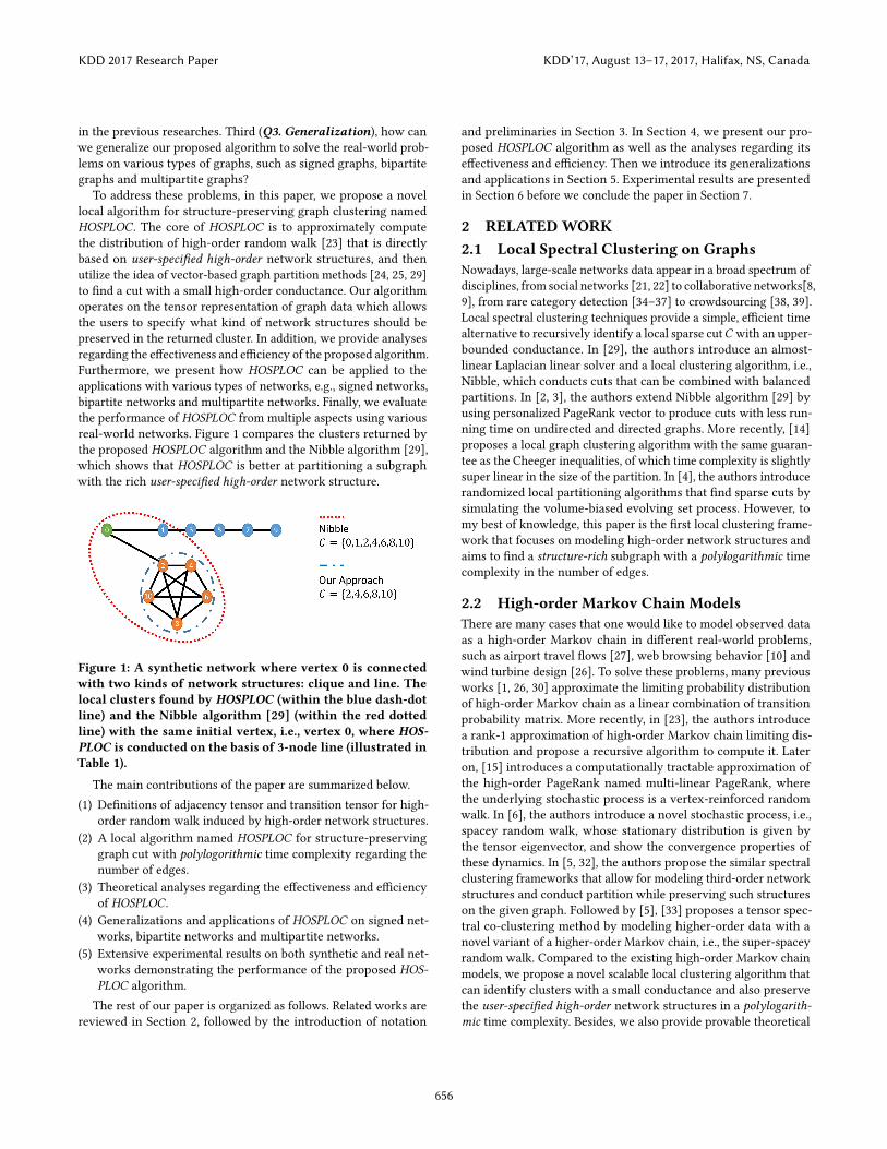
real-world networks. Figure 1 compares the clusters returned by

the proposed HOSPLOC algorithm and the Nibble algorithm [29],

which shows that HOSPLOC is better at partitioning a subgraph

with the rich user-specified high-order network structure.

Figure 1: A synthetic network where vertex 0 is connected

with two kinds of network structures: clique and line. The

local clusters found by HOSPLOC (within the blue dash-dot

line) and the Nibble algorithm [29] (within the red dotted

line) with the same initial vertex, i.e., vertex 0, where HOS-

PLOC is conducted on the basis of 3-node line (illustrated in

Table 1).

The main contributions of the paper are summarized below.

(1) Definitions of adjacency tensor and transition tensor for high-

order random walk induced by high-order network structures.

(2) A local algorithm named HOSPLOC for structure-preserving

graph cut with polylogorithmic time complexity regarding the

number of edges.

(3) Theoretical analyses regarding the effectiveness and efficiency

of HOSPLOC.(4) Generalizations and applications of HOSPLOC on signed net-

works, bipartite networks and multipartite networks.

(5) Extensive experimental results on both synthetic and real net-

works demonstrating the performance of the proposed HOS-PLOC algorithm.

The rest of our paper is organized as follows. Related works are

reviewed in Section 2, followed by the introduction of notation

and preliminaries in Section 3. In Section 4, we present our pro-

posed HOSPLOC algorithm as well as the analyses regarding its

effectiveness and efficiency. Then we introduce its generalizations

and applications in Section 5. Experimental results are presented

in Section 6 before we conclude the paper in Section 7.

2 RELATED WORK

2.1 Local Spectral Clustering on Graphs

Nowadays, large-scale networks data appear in a broad spectrum of

disciplines, from social networks [21, 22] to collaborative networks[8,

9], from rare category detection [34–37] to crowdsourcing [38, 39].

Local spectral clustering techniques provide a simple, efficient time

alternative to recursively identify a local sparse cutC with an upper-

bounded conductance. In [29], the authors introduce an almost-

linear Laplacian linear solver and a local clustering algorithm, i.e.,

Nibble, which conducts cuts that can be combined with balanced

partitions. In [2, 3], the authors extend Nibble algorithm [29] by

using personalized PageRank vector to produce cuts with less run-

ning time on undirected and directed graphs. More recently, [14]

proposes a local graph clustering algorithm with the same guaran-

tee as the Cheeger inequalities, of which time complexity is slightly

super linear in the size of the partition. In [4], the authors introduce

randomized local partitioning algorithms that find sparse cuts by

simulating the volume-biased evolving set process. However, to

my best of knowledge, this paper is the first local clustering frame-

work that focuses on modeling high-order network structures and

aims to find a structure-rich subgraph with a polylogarithmic time

complexity in the number of edges.

2.2 High-order Markov Chain Models

There are many cases that one would like to model observed data

as a high-order Markov chain in different real-world problems,

such as airport travel flows [27], web browsing behavior [10] and

wind turbine design [26]. To solve these problems, many previous

works [1, 26, 30] approximate the limiting probability distribution

of high-order Markov chain as a linear combination of transition

probability matrix. More recently, in [23], the authors introduce

a rank-1 approximation of high-order Markov chain limiting dis-

tribution and propose a recursive algorithm to compute it. Later

on, [15] introduces a computationally tractable approximation of

the high-order PageRank named multi-linear PageRank, where

the underlying stochastic process is a vertex-reinforced random

walk. In [6], the authors introduce a novel stochastic process, i.e.,

spacey random walk, whose stationary distribution is given by

the tensor eigenvector, and show the convergence properties of

these dynamics. In [5, 32], the authors propose the similar spectral

clustering frameworks that allow for modeling third-order network

structures and conduct partition while preserving such structures

on the given graph. Followed by [5], [33] proposes a tensor spec-

tral co-clustering method by modeling higher-order data with a

novel variant of a higher-order Markov chain, i.e., the super-spacey

random walk. Compared to the existing high-order Markov chain

models, we propose a novel scalable local clustering algorithm that

can identify clusters with a small conductance and also preserve

the user-specified high-order network structures in a polylogarith-mic time complexity. Besides, we also provide provable theoretical


656

bounds on the effectiveness and efficiency of the proposed HOS-PLOC algorithm.

3 NOTATIONS AND PRELIMINARIES

In this section, we review the basics of random walks with the

Markov chain interpretation and the Nibble algorithm for local

clustering on graphs [29], which pave the way for the proposed

structure-preserving graph cut algorithm to be introduced in the

next section.

3.1 Notations

Given an undirected graph G = (V ,E), where V consists of n ver-

tices, and E consists ofm edges, we let A ∈ Rn×n denote the ad-

jacency matrix of graph G, D ∈ Rn×n denote the diagonal matrix

of vertex degrees, and d(v) = D(v,v) denote the degree of vertexv ∈ V . The transition matrix of a lazy random walk on graph Gis M = (ATD−1 + I )/2, where I ∈ Rn×n is an identity matrix. For

convenience, we define the indicator vector χC as follows.

χC (v) =

{1 v ∈ C

0 Otherwise

.

In particular, the initial distribution of a random walk starting from

vertex v could be denoted as χv .The volume of a subset C ⊆ V is defined as the summation of

vertex degrees inC , i.e., µ(C) =∑v ∈C d(v). We let C̄ be the comple-

mentary set of C , i.e., C̄ = {v ∈ C̄ |v ∈ V ,v < C}. The conductance

of subset C ⊆ V is therefore defined as Φ(C) = |E(C,C̄) |

min(µ(C),µ(C̄))[7],

where E(C, C̄) = {(u,v)|u ∈ C,v ∈ C̄}, and |E(C, C̄)| denotes thenumber of edges in E(C, C̄). Besides, we represent the elements in

a matrix or a tensor using the convention similar to Matlab, e.g.,

M(i, j) is the element at the ith row and jth column of the matrix

M , andM(i, :) is the ith row ofM , etc.

3.2 Markov Chain Interpretation

The oth order Markov chain S describes a stochastic process that

satisfies [15]

Pr (St+1 = i1 |St = i2, . . . , St−o+1 = io+1, . . . , S1 = it+1)

=Pr (St+1 = i1 |St = i2, . . . , St−o+1 = io+1)(1)

where i1, . . . , it+1 denote the set of states associated with differ-

ent time stamps. Specifically, this means the future state only de-

pends on the past o states. If each vertex in graph G corresponds

to a distinct state, we can interpret the transition matrixM as the

transition matrix of the 1st-order Markov chain. Specifically, the

transition probability between vertex i and vertex j is given by

M(i, j) = Pr (St+1 = i |St = j). In Section 4.1, we introduce the idea

of adjacency tensor and transition tensor for modeling the high-

order network structures, which will lead to the high-order Markov

chains and high-order random walks.

3.3 Nibble Algorithm

Given an undirected graph G and a parameter ϕ > 0, to find a cut

C from G such that Φ(C) ≤ ϕ or to determine no such C exists is

an NP-complete problem [28]. Nibble algorithm [29] is one of the

earliest attempts to partition a graph with a bounded conductance

in polylogarithmic time. Starting from a given vertex, Nibble prov-

ably finds a local cluster in time (O(2bloд6m)/ϕ4)), where b is a

constant which controls the lower bound of the output volume.

This is proportional to the size of the output cluster. The key idea

behind Nibble is to conduct truncated random walks by using the

following truncation operator

[q]ϵ (u) =

{q(u) if q(u) ≥ d(u)ϵ

0 Otherwise

(2)

where q ∈ Rn is the distribution vector over all the vertices in the

graph, and ϵ is the truncation threshold that can be computed as

follows [29]

ϵ =1

(1800 · (l + 2)tlast 2b )

(3)

where l can be computed as l = ⌈loд2(µ(V )/2)⌉, and tlast can be

computed as tlast = (l + 1)⌈2

ϕ2ln

(c1(l + 2)

√µ(V )/2

)⌉.

Then, Nibble applies the vector-based partition method [24, 25,

29] that sorts the probable nodes based on the ratio of function

Ix to produce a low conductance cut. To introduce function Ixmathematically, we first define Sj (q) to be the set of top j vertices uthat maximizes q(u)/d(u). That is Sj (q) = {π (1), . . . ,π (j)}, where

π is the permutation that followsq(π (i))d (π (i)) ≥

q(π (i+1))d (π (i+1)) . In addition,

we let λj (q) =∑u ∈Sj (q) d(u) denote the volume of the set Sj (q).

Finally, the function Ix is defined as follows

Ix (q, λj (q)) =q(π (i))

d(π (i)). (4)

In the next section, we will introduce the high-order structure

preserving graph cut framework, i.e., HOSPLOC. Compared to Nib-

ble, HOSPLOC can model the user-specified network structure and

conduct a structure-rich cut with a small conductance. Moreover,

similar to Nibble, HOSPLOC runs in polylogarithmic time with

respect to the number of edges in the graph.

4 HIGH-ORDER NETWORK STRUCTURE

AND THE HOSPLOC ALGORITHM

In the previous section, we introduced the notations and prelimi-

naries. Now, we generalize the idea of truncated local clustering to

produce clusters that preserve the user-specified high-order networkstructures. We start by introducing the adjacency tensor and the

associated transition tensor based on the user-specified high-ordernetwork structures, followed by the discussion on the stationary

distribution of high-order random walk. Then, we introduce the

definitions of high-order conductance and high-order diffusion core.

Finally, we present the proposed high-order local clustering algo-

rithm HOSPLOC with theoretical analyses on the effectiveness and

efficiency.

4.1 Adjacency Tensor and Transition Tensor

For an undirected graph G, the corresponding adjacency matrix Acould be considered as a matrix representation of the existing edges

on G . However, in many real applications, we may want to explore

and capturemore complex and high-order network structures. Table

1 summarizes the examples of network structures N of different

orders and the corresponding Markov chain. Notice that the order


657

N Example Illustration Markov Chain

1st-order Vertex

0th-order

2nd-order Edge

1st-order

3rd-order

3-node Line

2nd-order

Triangle

kth-order k-node Star (k − 1)th-order

Table 1: Network Structures N and Markov Chains.

of the network structure is different from the order of the Markov

chain (or random walk). For example, the edges in E are considered

as the 2nd-order network structures, and they correspond to the 1

st-

orderMarkovChain (randomwalk) due to thematrix representation

of E. We use k to denote the order of the network structure N.As what will be explained next, the kth-order network structures

correspond to the (k − 1)th-order Markov chain (random walk).

To model the user-specified network structure N, we introducethe definition of adjacency tensor T and the transition tensor P to

represent the high-order random walk induced by the high-order

network structures N.

Definition 4.1 (Adjacency Tensor). Given a graph G = (V ,E),

the kth-order network structure N on G could be represented in a

k-dimensional adjacency tensor T as follows

T (i1, i2, . . . , ik ) =

{1 {i1, i2, . . . , ik } ⊆ V and form N.

0 Otherwise.

(5)

Definition 4.2 (Transition Tensor). Given a graph G = (V ,E)

and the adjacency tensor T for the kth-order network structure N,the corresponding transition tensor P could be computed as

P(i1, i2, . . . , ik ) =T (i1, i2, . . . , ik )∑ni1=1T (i1, i2, . . . , ik )

(6)

By the above definition, we have

∑i1 P(i1, . . . , ik ) = 1. Therefore,

if each vertex inG is a distinguishable state, we can interpret thekth-

order transition tensor P as a (k −1)th-order Markov chain (random

walk), i.e., Pr (St+1 = i1 |St = i2, . . . , St−k+2 = ik ) = P(i1, . . . , ik ).Intuitively, if i1 , i

′1, and they both form N together with i2, . . . , ik ,

then the probabilities of the next state being i1 and being i ′1are

the same given St = i2, . . . , St−k+2 = ik . Notice that the transitionmatrixM of a lazy random walk defined in Subsection 3.1 can be

considered as a special case of Definition 4.2 with the 2nd-order

network structure N, if we allow self-loops.

4.2 Stationary Distribution

For the kth-order network structure N and the corresponding (k −

1)th-order random walk with transition tensor P, if the stationarydistribution X exists, where X is a (k − 1)-dimensional tensor, then

it satisfies [15]

X (i1, i2, . . . , ik−1) =∑ik

P(i1, i2, . . . , ik )X (i2, . . . , ik ). (7)

where X (i1, . . . , ik−1) denotes the probability of being at states

i1, . . . , ik−1 in consecutive time steps upon convergence of the

random walk, and

∑i1, ...,ik−1 X (i1, . . . , ik−1) = 1.

However, for this system, storing the stationary distribution re-

quires O(n(k−1)) space complexity. For the sake of computational

scalability, in high-order random walks, a commonly held assump-

tion is ‘rank-one approximation’ [5, 23], i.e.,

X (i2, . . . , ik ) = q(i2) . . .q(ik ) (8)

where q ∈ Rn×1+ with

∑i q(i) = 1. Then, we have∑

i2, ...,ik

P(i1, . . . , ik )q(i2) . . .q(ik ) = q(i1).

In this way, the space complexity of the stationary distribution

of high-order random walk is reduced to O(n). Although q is an

approximation of the true stationary distribution of the high-order

random walk, [23] theoretically demonstrates the convergence and

effectiveness of the nonnegative vector q if P satisfies certain prop-

erties.

Following [5, 23], in this paper, we also adopt ‘rank-one approx-

imation’ and assume the stationary distribution of the high-order

random walk satisfies Eq. 8. To further simplify the notation, we let

P̄ denote the (k − 2)-mode unfolding matrix of the k-dimensional

transition tensor P . Thus, the (k − 1)th-order random walk satisfies:

q = P̄(q ⊗ . . . ⊗ q) (9)

where ⊗ denotes the Kronecker product symbol. For example, for

the third-order network structure N (e.g., triangle), the transition

tensor P ∈ Rn×n×n can be constructed based on Definition 4.2.

Then, the 1-mode unfolding matrix P̄ of P can be written as follows

P̄ = [P(:, :, 1), P(:, :, 2), . . . , P(:, :,n)]

where P̄ ∈ Rn×n2

. In this way, the associated second-order random

walk with respect to the triangle network structure satisfies

q = P̄(q ⊗ q).

4.3 High-Order Conductance

Given a high-order network structure N, it is usually the case that

the user would like to find a local clusterC on the graphG such that:

(1)C contains a rich set of network structures N; (2) by partitioningall the vertices into C and C̄ , we do not break many such network

structures. For example, in financial fraud detection, directed loops

may refer to money laundering activities. In this case, we want to

ensure the partition preserves rich directed loops inside the cluster

and breaks such structure as less as possible. It is easy to see that

the traditional definition of the conductance Φ(C) introduced in

Subsection 3.1 does not serve this purpose. Therefore, we introduce

the following generalized definition of conductance to preserve

user-defined high-order network structure N.


658

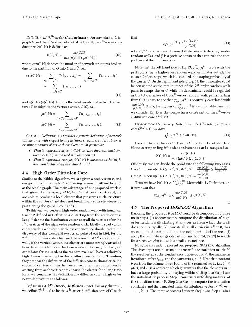
Definition 4.3 (kth-order Conductance). For any cluster C in

graph G and the kth-order network structure N, the kth-order con-ductance Φ(C,N) is defined as

Φ(C,N) =cut(C,N)

min{µ(C,N), µ(C̄,N)}(10)

where cut(C,N) denotes the number of network structures broken

due to the partition of G into C and C̄ , i.e.,

cut(C,N) =∑

i1, ...,ik ∈VT (i1, . . . , ik ) −

∑i1i2, ...,ik ∈C

T (i1, . . . , ik )

−∑

i1, ...,ik ∈C̄

T (i1, . . . , ik )

(11)

and µ(C,N) (µ(C̄,N)) denotes the total number of network struc-

tures N incident to the vertices within C (C̄), i.e.,

µ(C,N) =∑

i1∈C ;i2, ...,ik ∈VT (i1, i2, . . . , ik )

µ(C̄,N) =∑

i1∈C̄ ;i2, ...,ik ∈V

T (i1, i2, . . . , ik ). (12)

Claim 1. Definition 4.3 provides a generic definition of networkconductance with respect to any network structure, and it subsumesexisting measures of network conductance. In particular.

• When N represents edges, Φ(C,N) is twice the traditional con-ductance Φ(C) introduced in Subsection 3.1.

• When N represents triangles, Φ(C,N) is the same as the ‘high-order conductance’ ϕ3 introduced in [5].

4.4 High-Order Diffusion Core

Similar to the Nibble algorithm, we are given a seed vertex v , andour goal is to find a cluster C containing or near v without looking

at the whole graph. The main advantage of our proposed work is

that, given the user-specified high-order network structure N, weare able to produce a local cluster that preserves such structure

within the cluster C and does not break many such structures by

partitioning the graph into C and C̄ .To this end, we perform high-order random walk with transition

tensor P defined in Definition 4.2, starting from the seed vertex v .

Let q(t ) denote the distribution vector over all the vertices after the

t th iteration of the high-order random walk. Ideally, a seed vertex

chosen within a cluster C with low conductance should lead to the

discovery of this cluster. However, as pointed out in [29], for the

2nd-order network structure and the associated 1

st-order random

walk, if the vertices within the cluster are more strongly attached

to vertices outside the cluster than inside it, they may not be good

candidates for the seed, as the random walk will have a relatively

high chance of escaping the cluster after a few iterations. Therefore,

they propose the definition of the diffusion core to characterize the

subset of vertices within the cluster, such that the random walks

starting from such vertices stay inside the cluster for a long time.

Here, we generalize the definition of a diffusion core to high-order

network structures as follows.

Definition 4.4 (kth-Order ξ -Diffusion Core). For any cluster C ,

we define Ck,ξ ∈ C to be the kth-order ξ -diffusion core of C , such

that

χTC̄k,ξ q(t ) ≤ ξ

cut(C,N)

µ(C,N)(13)

where q(t ) denotes the diffusion distribution of t-step high-order

random walks, and ξ is a positive constant that controls the com-

pactness of the diffusion core.

Note that the left hand side of Eq. 13, χTC̄k,ξ q

(t ), represents the

probability that a high-order random walk terminates outside the

clusterC after t steps, which is also called the escaping probability ofthe clusterC . On the right hand side of Eq. 13, the numerator could

be considered as the total number of the kth-order random walk

paths to escape clusterC , while the denominator could be regarded

as the total number of the kth-order random walk paths starting

from C . It is easy to see that χTC̄k,ξ q

(t )is positively correlated with

cut (C,N)µ(C,N) . Since, for a given C , χT

C̄k,ξ q(t )

is a computable constant,

we consider Eq. 13 as the compactness constraint for the kth-order

ξ -diffusion core Ck,ξ ∈ C .

Proposition 4.5. For any cluster C and the k th-Order ξ -diffusioncore Ck,ξ ∈ C , we have

χTC̄k,ξ q(t ) ≤ ξΦ(C,N). (14)

Proof. Given a clusterC ∈ V and a kth-order network structureN, the corresponding kth-order conductance can be computed as

Φ(C,N) =cut(C,N)

min{µ(C,N), µ(C̄,N)}.

Obviously, we can divide the proof into the following two cases.

Case 1 : when µ(C,N) ≥ µ(C̄,N), Φ(C,N) = cut (C,N)µ(C̄,N) ≥

cut (C,N)µ(C,N) .

Case 2 : when µ(C,N) < µ(C̄,N), Φ(C,N) = cut (C,N)µ(C,N) .

Thus, we haveΦ(C,N) ≥ cut (C,N)µ(C,N) . Meanwhile, byDefinition. 4.4,

it turns out that

χTC̄k,ξ q(t ) ≤ ξ

cut(C,N)

µ(C,N)≤ ξΦ(C,N).

�

4.5 The Proposed HOSPLOC Algorithm

Basically, the proposed HOSPLOC could be decomposed into three

main steps: (1) approximately compute the distribution of high-

order random walk starting at any vertex from which the walk

does not mix rapidly; (2) truncate all small entries in q(t ) to 0, thus

we can limit the computation to the neighborhood of the seed; (3)

apply the vector-based graph partition method [24, 25, 29] to search

for a structure-rich cut with a small conductance.

Now, we are ready to present our proposed HOSPLOC algorithm.

The given input are the transition tensor P, the transition matrixM ,

the seed vertex v , the conductance upper-bound ϕ, the maximum

iteration number tmax, and the constants b, c1, ξ . Note that constant

b controls the volume lower bound of the returned set C , i.e., 2b ≤

µ(C), and c1 is a constant which guarantees that the elements in Chave a large probability of staying within C . Step 1 to Step 4 are

the initialization process. Step 1 constructs unfolding matrix P̄ of

the transition tensor P. Step 2 to Step 4 compute the truncation

constant ϵ and the truncated initial distributions vectors r (m),m =

1, . . . ,k − 1. The iterative process between Step 5 and Step 16 aims


659

to identify the proper high-order local cluster C: Step 6 calculates

the updated distribution over all the vertices in current iteration;

Step 7 calculates the truncated local distribution r (t ); the iterativeprocess stops when it finds a proper cluster which satisfies the three

constraints in Step 9 to Step 11, where condition (a) guarantees thatthe conductance of C is upper-bounded by ϕ, condition (b) ensures

that the volume of C is lower-bounded by 2b, and condition (c)

enforces that elements in C have a large probability mass.

Algorithm 1 High-Order Structure-Preserved Local Cut (HOS-PLOC)Input:

(1) Transition tensor P and transition matrixM ,

(2) Initial vertex v ,(3) Conductance upper bound ϕ,(4) Maximum iteration number tmax,

(5) Parameters b, c1, ξ .Output:

Local cluster C;1: Construct the unfolding matrix P̄ of the transition tensor P.

2: Compute constant ϵ based on Eq. 3.

3: Set initial distribution vectors q(t ) = M(t−1)χv , where t =1, . . . ,k − 1.

4: Compute truncated initial local distribution vectors r (t ) =

[q(t )]ϵ , t = 1, . . . ,k − 1.

5: for t = k : tmax do

6: Update distribution vector q(t ) = P̄(r (t−1) ⊗ . . . ⊗ r (t−k+1)).

7: Update truncated distribution vectors r (t ) = [q(t )]ϵ .8: if there exists a j such that:

9: (a)Φ(Sj (q(t ))) <= ϕ,

10: (b)2b <= λj (q

(t )),

11: (c)Ix (q(t ), 2b ) >=

ξc1(l+2)2b

. then

12: return C = Sj (q(t )) and quit.

13: else

14: Return C = ∅.

15: end if

16: end for

Next, we analyze the proposed HOSPLOC algorithm in terms of

effectiveness and efficiency. Regarding the effectiveness, we will

show that for any cluster C , if the seed vertex comes from the kth-

order ξ -diffusion core, i.e., v ∈ Ck,ξ , then the non-empty set C ′

returned by HOSPLOC has a large overlap with C . To be specific,

we have the following theorem.

Theorem 4.6 (Effectiveness of HOSPLOC). LetC be a clus-ter on graph G such that Φ(C,N) ≤ 1

c2(l+2), where 2c1 ≤ c2. If HOS-

PLOC runs with starting vertex v ∈ Ck,ξ and returns a non-emptyset C ′, then we have µ(C ′ ∩C) ≥ 2

b−1.

Proof. Let q(t ), t ≤ tmax, be the distribution of t − step high-

order random walk when the set C ′ = Sj (q(t )) is obtained. Then,

based on Proposition 4.5, we have the following inequality

χTC̄q(t ) ≤ χTC̄k,ξ q

(t ) ≤ ξΦ(C,N) ≤ξ

c2(l + 2). (15)

In Step 11 of Algorithm 1, condition (c) guarantees that

Ix (u) =q(t )(u)

d(u)≥

ξ

c1(l + 2)2b(16)

where u ∈ Sj (q(t )). Since d(u) ≥ 0 and c1(l + 2)2

b ≥ 0, we can infer

the following inequality from Eq. 16

d(u) ≤1

ξc1(l + 2)2

bq(t )(u). (17)

Let j ′ be the smallest integer such that λj′(q(t )) ≥ 2

b. In Step 10

of Algorithm 1, condition (b) guarantees that j ′ ≤ j. By Eq. 15 and

Eq. 17, we have

µ(Sj′(q(t )) ∩ C̄)

=∑

u ∈Sj′ (q(t ))∩C̄

d(u)

≤∑

u ∈Sj′ (q(t ))∩C̄

1

ξc1(l + 2)2

bq(t )(u)

≤1

ξc1(l + 2)2

b (χTC̄q(t ))

≤ξc1(l + 2)2

b

ξc2(l + 2)≤ 2

b−1.

(18)

Due to 2b <= λ′j (q

(t )), it turns out that µ(Sj′(q(t )) ∩ C) ≥ 2

b−1.

Since j ≥ j ′, we have the final conclusion

µ(Sj (q(t )) ∩C) ≥ µ(Sj′(q

(t )) ∩C) ≥ 2b−1. (19)

�

Regarding the efficiency of HOSPLOC, we provide the followinglemma to show the polylogarithmic time complexity of HOSPLOCwith respect to the number of edges in the graph.

Lemma 4.7 (Efficiency of HOSPLOC). Given Graph G andthe k th-order network structure N, k ≥ 3, the time complexity of

HOSPLOC is bounded by O(tmax

2bk

ϕ2k loд3km

).

Proof. To bound the running time of HOSPLOC, we first showthat each iteration in Algorithm 1 takes time O( 1

ϵk). Instead of

conducting dense vector multiplication or Kronecker product, we

track the nonzeros in both matrixes and vectors. Here, we let V t

denote the set of vertices such that {u ∈ V (t ) |r (t )(u) > 0}, and

V (t̂ )be the set with the maximum number of nonzero elements

in {V (t ) |1 ≤ t ≤ tmax }. In Step 6, the Kronecker product chain

r (t−1) ⊗ . . . ⊗ r (t−k+1) can be performed in time proportion to

|V (t−1) | . . . |V (t−k+1) | ≤ |V (t̂ ) |(k−1) ≤ µ(V (t̂ ))(k−1).

Also, [29] shows that µ(V (t )) ≤ 1/ϵ for all t . Therefore, to compute

r (t−1) ⊗ . . . ⊗ r (t−k+1) takes O(µ(V (t̂ ))(k−1)) ≤ O(1/ϵ (k−1)) time.

After that, the matrix vector product can be computed in

O(µ(V (t ),N)) ≤ O(µ(V (t̂ ),N)) ≤ O(µ(V (t̂ )))k ≤ O(1

ϵk).

The truncation in Step 7 can be computed in time O(|V (t̂ ) |). Step

8 to Step 15 require sorting the vertices in |V t | according to r (t ),

which takes time O(|V (t̂ ) | log |V (t̂ ) |). In sum, the time complexity

of each iteration in HOSPLOC is O( 1

ϵk).


660

Since the algorithm runs at most tmax iterations, the overall

time complexity of HOSPLOC is O( tmaxϵk

). By Eq. 3, we can expand

O( tmax

ϵk) as follows

O

(tmax

ϵk

)= O

©«tmax

(2bloд3µ(V )

ϕ2

)k ª®¬ = O(tmax

2bk

ϕ2kloд3km

).

�

Remark 1: The major computation overhead of Algorithm 1

comes from Step 6. Note that O(tmax

2bk

ϕ2k loд3km

)is a strict upper-

bound for considering extreme cases. While, due to the power

law distribution in real networks, we may usually have |V (t ) | ≤√µ(V (t̂ )). Then, the time complexity of Algorithm 1 can be reduced

to O(tmax /ϵk/2) = O(tmax (2

b/ϕ2)k/2loд3k/2m).

Remark 2: Suppose the maximum iteration number of Nibble

and HOSPLOC are both upper-bounded by tmax , then the time

complexity of Nibble is O(tmax 2

b loд4mϕ2

). Considering the k = 3

case, the time complexity of HOSPLOC isO(tmax

23b

ϕ6loд9m

). With-

out considering the impact from the other constants, we can see

that similar to Nibble, HOSPLOC also runs in polylogarithmic time

complexity with respect to the number of edges in the graph.

5 GENERALIZATIONS AND APPLICATIONS

In this section, we will to introduce several generalizations and ap-

plications of our proposedHOSPLOC algorithm on signed networks,

bipartite networks and multipartite networks.

5.1 Community Detection on Signed Network

First, we extend our proposed framework, i.e., HOSPLOC, to solve

problems on signed graphs. In many real applications, the high-

order network structures of interest to us are presented with signed

edges. For instance, Fig. 2 presents an unstable 3-node network

structure and a stable 3-node network structure based on social

status theorem [17]. In community detection [13], we may want to

ensure (1) the stable configurations to be rich within communities

and sparse in-between different communities; (2) the unstable con-

figurations to be sparse within communities and rich in-between

different communities. For this purpose, the adjacency tensor can

be constructed as follows

T (i1, i2, . . . , ik ) =

1 {i1, i2, . . . , ik } is stable structure

0 {i1, i2, . . . , ik } is unstable structure

α Otherwise

(20)

where {i1, i2, . . . , ik } ∈ V and constant 0 < α < 1. By this way,

we can ensure: (1) the returned cluster of HOSPLOC contains rich

stable structures; (2) the partition would most likely break unstable

structures.

5.2 Adversarial Learning on Bipartite Network

We now turn our attention to the problem of user behavior mod-

eling on the adversarial networks. Given an adversarial network

B = (VB ,EB ), the bipartite graph B contains two types of nodes,

i.e., user nodes VU and advertiser campaign nodes VA, i.e., VB =

Figure 2: Social Status Theory Example: (Left) A directed “+"

edge from node v1 to node v2 shows that v2 has a higher sta-tus than v1. (Right) A directed “-" edge from node v1 to node

v2 shows vice versa.

{VU ,VA}. The edges EB only exist between user nodes VU and

advertiser campaign nodes VA. Intuitively, the customers with sim-

ilar activities on the adversarial network should be included in the

same cluster. For this reason, we choose 4-node loop as the base

network structure for HOSPLOC algorithm. Specifically, suppose

both user nodes u1, u2 have user-campaign interactions with the

advertiser campaign nodes a1 and a2, then we have a 4-node loop,

i.e., u1 → a1 → u2 → a2 → u1. In this problem, we consider

the adversarial network as an undirected graph, and the adjacency

tensor can be constructed as follows

T (i1, i2, i3, i4) =

{1 {i1, i2, i3, i4} form a 4-nodes loop

0 Otherwise

(21)

where {i1, i2, i3, i4} ∈ VB . Starting from an initial vertex, the re-

turned clusterCB byHOSPLOC would represent a local user-campaign

community, which consists of both similar users and the users’ fa-

vorite advertiser campaigns.

5.3 Synthetic ID Detection on Multipartite

Network

Now we will explain how to detect synthetic IDs on PII network by

using our proposed HOSPLOC algorithm. PII network is a typical

multipartite network, where each partite set of nodes represents a

particular type of PII, such as users’ names, users’ accounts, and

email addresses, and the edges only exist between different partite

sets of nodes. In synthetic ID fraud [18], criminals often use modi-

fied identity attributes, such as phone number, home address and

email address, to combine with real users’ information and create

synthetic IDs to do malicious activities. Hence, for the synthetic

IDs, there is a high possibility that their PIIs would be shared by

multiple identities, which may compose rich star-shaped structures.

In this case, the adjacency tensor can be constructed as

T (i1, i2, . . . , ik ) =

{1 {i1, i2, . . . , ik } form a k-node star

0 Otherwise

(22)

where {i1, i2, . . . , ik } ∈ VB . Note that the returned partition may

consist of various types of nodes. However, it is viable to trace

back from the extracted PII nodes and discover the set of synthetic

identities.

6 EXPERIMENTAL RESULTS

Now, we demonstrate the performance of our proposed HOSPLOCalgorithm in the sense of effectiveness, efficiency, and parameter


661

(a) Conductance (b) The 3rd-Order Conductance (c) Triangle Density

Figure 3: Effectiveness.

sensitivity. Moreover, we also present two interesting case studies

on bipartite graph and multipartite graph.

6.1 Experiment Setup

Category Network Type Nodes Edges

Citation Author Undirected 61,843 402,074

Paper Undirected 62,602 10,904

Infrastructure Airline Undirected 2,833 15,204

Oregon Undirected 7,352 15,665

Power Undirected 4,941 13,188

Social Epinion Undirected 75,879 508,837

Review Rating Bipartite 8724 90962

Financial PII Multipartite 375 519

Table 2: Statistics of the Networks.

Data sets: We evaluate our proposed algorithm on both synthetic

and real-world network graphs. The statistics of all real data sets

are summarized in Table 2.

• Collaboration Network: We use two collaboration networks from∗.

In network (Author), the nodes are authors, and an edge only

exists when two authors have a co-authored paper. In network

(Paper), the nodes are distinct papers, and an edge only exists

when one paper cites another paper.

• Infrastructure Network: In network (Airline)†, the nodes represent

2,833 airports, and the edges represent the U.S. flights in a one-

month interval. Network (Oregon) [20] is a network of routers in

Autonomous Systems inferred from Oregon route-views between

March 31, 2001, and May 26, 2001. Network (Power)‡contains

the information of the power grid of the western states of U.S. A

node represents a generator, a transformator or a substation, and

an edge represents a power supply line.

• Social Network: Network (Epinion) [20] is a who-trust-whom

online social network. Each node represents a user, and one edge

exits if and only if when one user trusts another user.

• Review Network: Network (Rating) [16] is a bipartite graph, whereone side of nodes represent 643 users, and another side of nodes

represent 7,483 movies. Edges refer to the positive ratings, i.e.,

rating score larger than 2.5, on MovieLens website. Note that

this network is a subgraph from the original one, due to storing

∗https://aminer.org/data

†http://www.levmuchnik.net/Content/Networks/ NetworkData.html

‡http://konect.uni-koblenz.de/networks/opsahl-powergrid

the 4th-order transition tensor of the original graph, i.e., 100s K

vertices and millions edges, requires too much memory.

• Financial Network: Network (PII) is a multipartite graph, which

consists of five types of vertices, i.e., 112 bank accounts, 71 names,

80 emails, 35 addresses, and 77 phone numbers. Edges only exist

between account vertices and PII vertices.

Comparison Methods: In our experiments, we compare our

methods with both local and global graph clustering methods.

Specifically, the comparison algorithm includes three local algo-

rithms, i.e., (1) Nibble [29]; (2) NPR [2]; (3) LS-OQC [31], and two

global clustering algorithms, i.e., (1) NMF [12]; (2) TSC [5]. Among

these five baseline algorithms, TSC algorithm is designed based on

high-order Markov chain, which can model high-order network

structures, i.e., triangle.

Repeatability: Most of the data sets are publicly available. The

code of the proposed algorithms will be released on the authors’

website. For all the results reported, we set c1 = 140 and ξ = 1. The

experiments are mainly performed on a Windows machine with

four 3.5GHz Intel Cores and 256GB RAM.

6.2 Effectiveness Comparison

The effectiveness comparison results conducted on six real undi-

rected graphs by the following three evaluation metrics are shown

in Fig. 3. Among them, (1) Conductance [7] measures the general

quality of a cut on graph, which quantitatively indicates the com-

pactness of a cut; (2) The 3rd-Order Conductance could be com-

puted based on Eq. 10 by treating triangle as the network structure

N, which estimates how well the network structure N is preserved

in the returned cut from being broken by the partitions; (3) Tri-

angle Density [7] computes the ratio of how rich the triangle is

included in the returned cluster.

Moreover, to evaluate the convergence of local algorithms, we

randomly select 30 vertices from one cluster on each testing graph

and run all the local algorithms multiple times by treating each of

these nodes as an initial vertex. In Fig. 3, the heights of bars indicate

the average value of evaluation metrics, and the error bars (only

for local algorithms) represent the standard deviation of evaluation

metrics in multiple runs. We have the following observations: (1) In

general, local algorithms perform better than the global algorithm,

and our HOSPLOC algorithm consistently outperforms the others

on all the evaluation metrics. For example, compared to the best

competitor, i.e., TSC, on network (Airline), HOSPLOC algorithm is


662

97% smaller on conductance, 12.2% smaller on the 3rd-order con-

ductance, 80% larger on triangle density. (2) High-order Markov

chain models, i.e., HOSPLOC and TSC, could better preserve tri-

angles in the returned cluster. For example, on network (Epinion),

both HOSPLOC and TSC return a cluster with much higher triangle

density and much lower the 3rd-order conductance. (3) HOSPLOC

algorithm shows a more robust convergence property than the

other local clustering algorithm by comparing the size of error bars.

For example, among the three local algorithms, only HOSPLOCalgorithm returns the identical cluster on network (Paper) with

different initial vertexes.

(a) The number of vertices (b) The lower bound of C’s volume

Figure 4: Scalability Analysis.

6.3 Scalability Analysis

Here, we evaluate the efficiency of our proposed HOSPLOC algo-

rithmwith triangle as the specified network structure, by comparing

with Nibble algorithm on synthetic graphs. Since our method is

built on higher order of random walk than Nibble, we consider

Nibble as the running time lower bound of HOSPLOC algorithm.

Notice that all the results in Fig. 4 are the average values of multiple

runs by using 30 different initial vertexes on the same graph. In

Fig. 4 (a), we show the running time of HOSPLOC and Nibble on a

series of synthetic graphs with increasing number of vertices but

fixed edge density of 0.5%. We observe that although HOSPLOCrequires more time than Nibble in each run, the running time of

HOSPLOC increases polylogarithmically with the size of the graph

|V |. In Fig. 4 (b), we show the running time of HOSPLOC and Nibble

versus the lower bound of output volume on the synthetic graph

with 5000 vertices and 0.5% edge density, by keeping the other

parameters fixed. We can see that the running time of HOSPLOC is

polynomial with respect to 2b, which is consistent with our time

complexity analysis.

(a) Conductance (b) The 3rd-order conductance

Figure 5: Parameter Analysis w.r.t. Conductance Upper-

bound ϕ.

6.4 Parameter Analysis

In this subsection, we analyze the parameter sensitivity of our pro-

posed HOSPLOC algorithm with triangle as the specified network

structure, by comparing with Nibble algorithm on the synthetic

graph with 5000 vertices and 0.5% edge density. In the experiments,

we evaluate the conductance and the 3rd-order conductance of the

returned cut with different values of input parameter ϕ. In Fig. 5, wehave the following observations: (1) HOSPLOC returns the optimal

cut even with a very lose conductance upper bound ϕ. In Fig. 5 (a),

we can see the output conductance of HOSPLOC converges to the

minimum value when ϕ = 0.4, while the output conductance of

Nibble converges to its minimum value until ϕ = 0.1. (2) Both the

conductance and the 3rd-order conductance of HOSPLOCś cut are

always smaller than Nibble’s cut with different ϕ.

6.5 Case Study

In this subsection, we will consider more complex network struc-

tures and perform our proposed HOSPLOC algorithm on bipartite

and multipartite networks.

Figure 6: Case study on bipartite network Rating. (a) An ex-

ample of detected community by HOSPLOC on Rating. (b)

An example of 4-node loop on Rating.

Case Study on Bipartite Graph.We conduct a case study on

the network (Rating) to find a local community consisting of sim-

ilar taste users and their favorite movies. In this case study, we

construct the transition tensor on the basis of 4-node loop based

on Eq. 21. Fig. 6 (a) presents a miniature of the cluster identified

by our proposed HOSPLOC algorithm regarding 4-node loop that

illustrated in Fig. 6 (b). For example, in Fig. 6, the highlighted red

loop shows that both of the third and the fourth users like the first

and the fourth movies, while the highlighted blue loop represents

that both of the third and the fifth users like the fifth and the last

movies. It seems the fifth user does not like the first movie due to

no direct connection between them. While the interesting part is

the first, the fifth and the last movies are from the same series, i.e.,

Karate Kid I, II, III. Moreover, the fourth movie, i.e., Back to School,

and Karate Kid I, II, III, are all from the category of comedy. It turns

out that our HOSPLOC algorithm returns a community of comedy

movies and their fans.

Case Study on Multipartite Graph. Here, we conduct a case

study on the network (PII) to identify suspicious systemic IDs. In

this case, we treat 5-node star as the underlying network struc-

ture, and the corresponding transition tensor could be generated


663

by Eq. 22. Fig. 7 (a) presents a subgraph of the returned cut by

our proposed HOSPLOC algorithm regarding 5-node star that illus-

trated in Fig. 7 (b). We can see that many PIIs are highly shared by

different accounts. For example, the account connected with blue

lines shares the home address and email address with the account

connected with purple lines, while the account connected with red

lines shares the holder’s name and phone number with the account

connected with blue lines. Comparing with the regular dense sub-

graph detection methods, our method can better identify the IDs

who share their PIIs with others, by exploring the nature structure

of PII, i.e., 5-node star, on the given graph.

Figure 7: Case study on multipartite network PII. (a) An ex-

ample of detected community by HOSPLOC on PII. (b) An

example of 5-node star on PII.

7 CONCLUSION

In this paper, we propose a local clustering framework, i.e., HOS-PLOC, that gives users the flexibility to model any high-order net-

work structures and returns a small high-order conductance cluster

which largely preserves the user-specified network structures. Be-

sides, we analyze its performance in terms of the optimality of the

obtained cluster and the polylogarithmic time complexity on mas-

sive graphs. Furthermore, we generalize the proposed HOSPLOCalgorithm and try to solve multiple real problems on signed net-

works, bipartite networks and multipartite networks, by exploring

the useful high-order network connectivity patterns, such as loops

and stars. Finally, the extensive empirical evaluations on a diverse

set of networks demonstrate the effectiveness and scalability of our

proposed HOSPLOC algorithm.

ACKNOWLEDGMENT

This work is supported by National Science Foundation under Grant

No. IIP-1430144, No. IIS-1552654 and No. IIS-1651203, ONR un-

der Grant No. N00014-15-1-2821 and No. N00014-16-1-2015, DTRA

under Grant No. HDTRA1-16-0017, Army Research Office under

the contract number No. W911NF-16-1-0168, National Institutes

of Health under the grant number No. R01LM011986, Region II

University Transportation Center under the project number No.

49997-33 25, an IBM Faculty Award and a Baidu gift.

REFERENCES

[1] SR A and SR D. 1988. Limit distribution of a high order Markov chain. J R StatSoc (1988).

[2] R. Andersen, F. Chung, and K. Lang. 2006. Local graph partitioning using pagerank

vectors. In IEEE FOCS (2006).

[3] R. Andersen, F. Chung, and K. Lang. 2007. Local partitioning for directed graphs

using PageRank. In International Workshop on Algorithms and Models for theWeb-Graph. Springer.

[4] R. Andersen, S. O. Gharan, Y. Peres, and L. Trevisan. 2016. Almost Optimal Local

Graph Clustering Using Evolving Sets. JACM (2016).

[5] A. R Benson, D. F Gleich, and J. Leskovec. 2015. Tensor spectral clustering for

partitioning higher-order network structures. In SIAM SDM (2015).[6] A. R Benson, D. F Gleich, and L.-H. Lim. 2016. The Spacey Random Walk: A

stochastic Process for Higher-Order Data. arXiv preprint arXiv:1602.02102 (2016).[7] B Bollobás. 2013. Modern graph theory. Springer Science & Business Media

(2013).

[8] C. Chen, J. He, N. Bliss, and H. Tong. 2015. On the connectivity of multi-layered

networks: Models, measures and optimal control. In IEEE ICDM (2015).[9] C. Chen, H. Tong, L. Xie, L. Ying, and Q. He. 2016. FASCINATE: Fast Cross-Layer

Dependency Inference on Multi-layered Networks. In ACM SIGKDD (2016).[10] F. Chierichetti, R. Kumar, P. Raghavan, and T. Sarlos. 2012. Are web users really

markovian?. In ACM WWW (2012).[11] K.-K. R. Choo. 2008. Money laundering risks of prepaid stored value cards. Aus-

tralian Institute of Criminology (2008).

[12] C. Ding, T. Li, and M. I Jordan. 2008. Nonnegative matrix factorization for

combinatorial optimization: Spectral clustering, graph matching, and clique

finding. In IEEE ICDM (2008).[13] S. Fortunato. 2010. Community detection in graphs. Physics reports (2010).[14] S. O. Gharan and L. Trevisan. 2012. Approximating the expansion profile and

almost optimal local graph clustering. In IEEE FOCS (2012).[15] D. F Gleich, L.-H. Lim, and Y. Yu. 2015. Multilinear PageRank. SIMAX (2015).

[16] F M. Harper and J. A Konstan. 2016. The movielens datasets: History and context.

TiiS (2016).[17] A. B Hollingshead et al. 1975. Four factor index of social status. (1975).

[18] C. J. Hoofnagle. 2007. Identity theft: Making the known unknowns known. Harv.JL & Tech. (2007).

[19] T. Leighton and S. Rao. 1999. Multicommodity max-flow min-cut theorems and

their use in designing approximation algorithms. JACM (1999).

[20] J. Leskovec and A. Krevl. 2014. SNAP Datasets: Stanford Large Network Dataset

Collection. http://snap.stanford.edu/data. (June 2014).

[21] J. Li, H. Dani, X. Hu, and H. Liu. 2017. Radar: Residual Analysis for Anomaly

Detection in Attributed Networks. In IJCAI (2017).[22] J. Li, X. Hu, L. Jian, and H. Liu. 2016. Toward Time-Evolving Feature Selection

on Dynamic Networks. In IEEE ICDM (2016).[23] W. Li and M. K Ng. 2014. On the limiting probability distribution of a transition

probability tensor. Linear and Multilinear Algebra (2014).[24] L. Lovász and M. Simonovits. 1990. The mixing rate of Markov chains, an

isoperimetric inequality, and computing the volume. In IEEE FOCS (1990).[25] L. Lovász and M. Simonovits. 1993. Random walks in a convex body and an

improved volume algorithm. Random structures & algorithms (1993).[26] A. E Raftery. 1985. A model for high-order Markov chains. J R Stat Soc Series B

Stat Methodol (1985).[27] M. Rosvall, A. V Esquivel, A. Lancichinetti, J. D West, and R. Lambiotte. 2014.

Memory in network flows and its effects on spreading dynamics and community

detection. Nature communications (2014).[28] J. Šíma and S. E. Schaeffer. 2006. On the NP-completeness of some graph cluster

measures. In Springer SOFSEM (2006).[29] D. A Spielman and S.-H. Teng. 2013. A local clustering algorithm for massive

graphs and its application to nearly linear time graph partitioning. SICOMP(2013).

[30] J. L Teugels. 2008. Markov Chains: Models, Algorithms and Applications. JASA(2008).

[31] C. Tsourakakis, F. Bonchi, A. Gionis, F. Gullo, and M. Tsiarli. 2013. Denser than

the densest subgraph: extracting optimal quasi-cliques with quality guarantees.

In ACM SIGKDD (2013).[32] C. E Tsourakakis, J. Pachocki, and M. Mitzenmacher. 2017. Scalable motif-aware

graph clustering. InWWW (2017).[33] T. Wu, A. R Benson, and D. F Gleich. 2016. General tensor spectral co-clustering

for higher-order data. In NIPS (2016).[34] D. Zhou, J. He, K.-S. Candan, and H. Davulcu. 2015. MUVIR: Multi-View Rare

Category Detection.. In IJCAI (2015).[35] D. Zhou, J. He, Y. Cao, and J. Seo. 2016. Bi-level Rare Temporal Pattern Detection.

In IEEE ICDM (2016).[36] D. Zhou, A. Karthikeyan, K. Wang, N. Cao, and J. He. 2016. Discovering rare

categories from graph streams. Springer DMKD (2016).

[37] D. Zhou, K. Wang, N. Cao, and J. He. 2015. Rare category detection on time-

evolving graphs. In IEEE ICDM (2015).[38] Y. Zhou and J. He. 2016. Crowdsourcing via tensor augmentation and completion.

In IJCAI (2016).[39] Y. Zhou, L. Ying, and J. He. 2017. MultiC2: an Optimization Framework for

Learning from Task and Worker Dual Heterogeneity. In SIAM SDM (2017).


664

http://snap.stanford.edu/data

A Local Algorithm for Structure-Preserving Graph Cut

Documents