A Linear Framework for Time-Scale Separation in Nonlinear Biochemical Systems Jeremy Gunawardena* Department of Systems Biology, Harvard Medical School, Boston, Massachusetts, United States of America Abstract Cellular physiology is implemented by formidably complex biochemical systems with highly nonlinear dynamics, presenting a challenge for both experiment and theory. Time-scale separation has been one of the few theoretical methods for distilling general principles from such complexity. It has provided essential insights in areas such as enzyme kinetics, allosteric enzymes, G-protein coupled receptors, ion channels, gene regulation and post-translational modification. In each case, internal molecular complexity has been eliminated, leading to rational algebraic expressions among the remaining components. This has yielded familiar formulas such as those of Michaelis-Menten in enzyme kinetics, Monod-Wyman- Changeux in allostery and Ackers-Johnson-Shea in gene regulation. Here we show that these calculations are all instances of a single graph-theoretic framework. Despite the biochemical nonlinearity to which it is applied, this framework is entirely linear, yet requires no approximation. We show that elimination of internal complexity is feasible when the relevant graph is strongly connected. The framework provides a new methodology with the potential to subdue combinatorial explosion at the molecular level. Citation: Gunawardena J (2012) A Linear Framework for Time-Scale Separation in Nonlinear Biochemical Systems. PLoS ONE 7(5): e36321. doi:10.1371/ journal.pone.0036321 Editor: Kumar Selvarajoo, Keio University, Japan Received March 3, 2012; Accepted March 29, 2012; Published May 14, 2012 Copyright: ß 2012 Jeremy Gunawardena. This is an open-access article distributed under the terms of the Creative Commons Attribution License, which permits unrestricted use, distribution, and reproduction in any medium, provided the original author and source are credited. Funding: The work described here was supported by the National Science Foundation under grant number 0856285. The funder had no role in study design, data collection and analysis, decision to publish, or preparation of the manuscript. Competing Interests: The author has declared that no competing interests exist. * E-mail: [email protected] Introduction The overwhelming molecular complexity of biological systems presents a formidable scientific challenge. The mere number of protein-coding genes barely captures this complexity, [1]. Tran- scription factor binding to DNA to regulate gene expression and protein post-translational modification, to mention just two well- studied mechanisms, enable combinatorial construction of vast numbers of molecular states, [2]. How such complexity evolves and how it gives rise to robust cellular physiology are among the central questions in biology. One of the few conceptual methods for rising above this complexity, and thereby distilling general principles, has been time-scale separation (Figure 1). A system of interest (dashed box) is identified, which, for a particular behaviour being studied, is assumed to contain all the components relevant to that behaviour. A sub-system (box) within the larger system is taken to be operating sufficiently fast that it may be assumed to have reached a steady state or, as a special case of that, a state of thermodynamic equilibrium. The larger system and its environment adjust on slower time-scales to the steady-state of the sub-system. The components within the sub-system may be viewed as ‘‘fast variables’’, while those additional components within the larger system are ‘‘slow variables’’. Those compo- nents in the environment that might be influenced by the overall system are taken to be operating on the slowest time scale. Such assumptions often enable the internal states of the sub-system to be eliminated, thereby simplifying the description of the larger system’s behaviour. Time-scale separation was first introduced at the molecular level in the famous work of Michaelis and Menten on enzyme kinetics, [3,4]. They considered the following biochemical reaction scheme, in which an enzyme, E, reversibly binds to a substrate, S, to form an intermediate enzyme-substrate complex, ES, which then irreversibly breaks up to form the product of the reaction, P, and release the enzyme: SzE'ES ?PzE : ð1Þ A time-scale separation was assumed in which the free enzyme, E, and the enzyme-substrate complex, ES, were regarded as fast variables, while S and P were regarded as slow variables. (As a matter of historical accuracy, Michaelis and Menten made a simpler rapid equilibrium assumption. The so-called ‘‘quasi steady-state’’ assumption used here, and now universally em- ployed, was first introduced by Briggs and Haldane, [5].) A simple algebraic calculation leads to the Michaelis-Menten rate formula d ½P dt ~ V max ½S K M z½S , ð2Þ in which the aggregated parameters V max and K M are determined by the underlying rate constants for the reactions in (1) and the total amount of enzyme that is present; see equation (9) below. Here, [X] denotes the concentration of the chemical species X. This example has two characteristic features. First, the algebra has eliminated the fast variables, E and ES, leaving a formula that PLoS ONE | www.plosone.org 1 May 2012 | Volume 7 | Issue 5 | e36321

Welcome message from author
This document is posted to help you gain knowledge. Please leave a comment to let me know what you think about it! Share it to your friends and learn new things together.
Transcript

A Linear Framework for Time-Scale Separation inNonlinear Biochemical SystemsJeremy Gunawardena*
Department of Systems Biology, Harvard Medical School, Boston, Massachusetts, United States of America
Abstract
Cellular physiology is implemented by formidably complex biochemical systems with highly nonlinear dynamics, presentinga challenge for both experiment and theory. Time-scale separation has been one of the few theoretical methods fordistilling general principles from such complexity. It has provided essential insights in areas such as enzyme kinetics,allosteric enzymes, G-protein coupled receptors, ion channels, gene regulation and post-translational modification. In eachcase, internal molecular complexity has been eliminated, leading to rational algebraic expressions among the remainingcomponents. This has yielded familiar formulas such as those of Michaelis-Menten in enzyme kinetics, Monod-Wyman-Changeux in allostery and Ackers-Johnson-Shea in gene regulation. Here we show that these calculations are all instances ofa single graph-theoretic framework. Despite the biochemical nonlinearity to which it is applied, this framework is entirelylinear, yet requires no approximation. We show that elimination of internal complexity is feasible when the relevant graph isstrongly connected. The framework provides a new methodology with the potential to subdue combinatorial explosion atthe molecular level.
Citation: Gunawardena J (2012) A Linear Framework for Time-Scale Separation in Nonlinear Biochemical Systems. PLoS ONE 7(5): e36321. doi:10.1371/journal.pone.0036321
Editor: Kumar Selvarajoo, Keio University, Japan
Received March 3, 2012; Accepted March 29, 2012; Published May 14, 2012
Copyright: � 2012 Jeremy Gunawardena. This is an open-access article distributed under the terms of the Creative Commons Attribution License, which permitsunrestricted use, distribution, and reproduction in any medium, provided the original author and source are credited.
Funding: The work described here was supported by the National Science Foundation under grant number 0856285. The funder had no role in study design,data collection and analysis, decision to publish, or preparation of the manuscript.
Competing Interests: The author has declared that no competing interests exist.
* E-mail: [email protected]
Introduction
The overwhelming molecular complexity of biological systems
presents a formidable scientific challenge. The mere number of
protein-coding genes barely captures this complexity, [1]. Tran-
scription factor binding to DNA to regulate gene expression and
protein post-translational modification, to mention just two well-
studied mechanisms, enable combinatorial construction of vast
numbers of molecular states, [2]. How such complexity evolves
and how it gives rise to robust cellular physiology are among the
central questions in biology.
One of the few conceptual methods for rising above this
complexity, and thereby distilling general principles, has been
time-scale separation (Figure 1). A system of interest (dashed
box) is identified, which, for a particular behaviour being
studied, is assumed to contain all the components relevant to
that behaviour. A sub-system (box) within the larger system is
taken to be operating sufficiently fast that it may be assumed to
have reached a steady state or, as a special case of that, a state
of thermodynamic equilibrium. The larger system and its
environment adjust on slower time-scales to the steady-state of
the sub-system. The components within the sub-system may be
viewed as ‘‘fast variables’’, while those additional components
within the larger system are ‘‘slow variables’’. Those compo-
nents in the environment that might be influenced by the
overall system are taken to be operating on the slowest time
scale. Such assumptions often enable the internal states of the
sub-system to be eliminated, thereby simplifying the description
of the larger system’s behaviour.
Time-scale separation was first introduced at the molecular level
in the famous work of Michaelis and Menten on enzyme kinetics,
[3,4]. They considered the following biochemical reaction scheme,
in which an enzyme, E, reversibly binds to a substrate, S, to form
an intermediate enzyme-substrate complex, ES, which then
irreversibly breaks up to form the product of the reaction, P,
and release the enzyme:
SzE'ES?PzE : ð1Þ
A time-scale separation was assumed in which the free enzyme, E,
and the enzyme-substrate complex, ES, were regarded as fast
variables, while S and P were regarded as slow variables. (As a
matter of historical accuracy, Michaelis and Menten made a
simpler rapid equilibrium assumption. The so-called ‘‘quasi
steady-state’’ assumption used here, and now universally em-
ployed, was first introduced by Briggs and Haldane, [5].) A simple
algebraic calculation leads to the Michaelis-Menten rate formula
d½P�dt
~Vmax ½S�
KMz½S� , ð2Þ
in which the aggregated parameters Vmax and KM are
determined by the underlying rate constants for the reactions in
(1) and the total amount of enzyme that is present; see equation (9)
below. Here, [X] denotes the concentration of the chemical
species X.
This example has two characteristic features. First, the algebra
has eliminated the fast variables, E and ES, leaving a formula that
PLoS ONE | www.plosone.org 1 May 2012 | Volume 7 | Issue 5 | e36321

involves only the slow variable, S, on the right hand side. In this
case, P does not appear on the right hand side because of the
irreversibility of (1). Second, the expression on the right hand side
is rational in the concentrations of the slow variables: it is a ratio of
two polynomials in [S]. In this simple case, both numerator and
denominator are first-order (linear) in [S].
Time-scale separations have been used in many distinct areas of
biology, including enzyme kinetics, allosteric enzymes, G-protein
coupled receptors, ligand-gated ion channels, gene regulation in
both prokaryotes and eukaryotes and protein post-translational
modification (see below). The characteristic features noted above,
of elimination leading to a rational expression, are shared by all of
them. Among these rational expressions are the familiar formulas
of Michaelis-Menten in enzyme kinetics, Monod-Wyman-Chan-
geux and Koshland-Nemethy-Filmer in allostery and Shea-Ackers-
Johnson in prokaryotic gene regulation. However, the correspond-
ing analyses have been largely independent and ad hoc. In this
paper we introduce a graph-theoretic framework that underlies all
of these analyses. Despite the biochemical nonlinearity of the
systems to which it is applied, the framework is entirely linear, yet
it is not an approximation. Moreover, it is symbolic in the values of
all rate constants, so that it may be used without having to know
these values in advance. We show that elimination of internal
complexity becomes feasible when the relevant graph is strongly
connected and that, in this case, rational expressions emerge which
can be explicitly described in terms of the graph. This procedure
accounts for the rational expressions arising in all the time-scale
separation examples just mentioned.
In these examples, time-scale assumptions have not always been
justified by data. Instead, time-scale separation has been used as a
hypothesis to simplify complex behaviour and thereby obtain new
insights, which have subsequently guided conceptual understand-
ing and experimental design. We follow the same practice here,
treating time-scale separation as a method of mathematical
simplification whose validity must ultimately be judged by its
conceptual usefulness in guiding new experiments.
The examples mentioned above are reviewed next, to show the
scope of application of the results and to point out some of the
experimental insights. We then introduce the linear framework
and explain how it underlies these different results. We also show
how the framework appears in the study of general biochemical
networks. Finally, as a demonstration of its power, we show how
the framework can be readily adapted to deal with the more
general situation in which a sub-system’s components are subject
to synthesis and degradation. Applications of the framework to
specific biological examples will be reported elsewhere.
Results
Examples of Time-scale SeparationEnzyme kinetics. Time-scale separation has been used to
analyse enzymes with multiple substrates, products and effectors.
As with the Michaelis-Menten formula in (2), the internal
complexity arising from the bound states of the enzyme can be
eliminated, leading to rational expressions involving only sub-
strates, products or effectors. The algebra was formalised in the
King-Altman procedure, [6], and the resulting rational expressions
have been widely used in biochemistry, [7,8]. For a modern
example, see [9].
Enzyme allostery. Balancing supply and demand in meta-
bolic networks requires enzymes to be controlled by molecules that
are structurally distinct from the enzyme’s substrate. Allosteric
regulation separates enzyme activity from control by exploiting
distinct enzyme conformations having distinct activities. A
molecule that binds preferentially to a conformation with weaker
activity is an inhibitor, while one that binds preferentially to a
conformation with stronger activity is an activator. Many enzymes
subject to such regulation are oligomers with an axis of symmetry.
A ‘‘concerted’’ model of enzyme allostery, in which the
conformational changes were assumed to be limited to symmetric
quaternary movements of the oligomer, was put forward in [10].
An independent ‘‘sequential’’ model, in which tertiary changes in
the individual monomers were also allowed, was put forward in
[11]. Subsequent formulations have allowed for additional
complexity, [12,13]. In each case, the enzyme conformations
and ligand binding are assumed to be at thermodynamic
equilibrium and the internal complexity arising from states with
multiple bound ligands is eliminated. Enzyme activity is usually
taken to be proportional to the equilibrium fractional saturation–
the proportion of sites that are bound by ligand–leading to rational
expressions such as the Monod-Wyman-Changeux formula, [10].
G-protein coupled receptors. GPCRs form the largest
signalling superfamily in the human genome and one of the most
clinically-significant, [14,15]. Pioneering quantitative studies of
the b2-adrenergic receptor showed that apparent low- and high-
affinity states of the receptor were explained by a ‘‘ternary
complex model’’, in which the receptor could be simultaneously
bound to both a ligand and an accessory protein, later shown to
be the G-protein, [16]. This basic model has been developed
further to include distinct (allosteric) receptor conformations,
[17,18], and remains widely influential in quantitative pharma-
cology, [19,20]. The possibility that distinct conformations recruit
distinct subsets of the downstream signalling network, has been
suggested as a basis for the phenomenon of collateral efficacy
(‘‘functional selectivity’’, ‘‘protean agonism’’, ‘‘stimulus traffick-
ing’’), [21], although post-translational modification of the
receptor may also play an important role (see below). In these
mathematical models of GPCRs, the conformational changes,
Figure 1. Schematic illustration of time-scale separation. Asystem is shown within the dashed box, which is assumed to contain allthe components relevant to a given behaviour, so that it is partiallyuncoupled from its environment: it influences its environment (arrowsleading outwards) but is not in turn influenced by the environment.Within the system is a smaller sub-system (box) which may be fullycoupled to the larger system (bi-directional arrows). The components inthe sub-system (blue dots) are taken to be operating sufficiently fastthat they may be assumed to have reached a steady state, or a state ofthermodynamic equilibrium, to which the remaining components in thelarger system (green dots), and those in the environment that areinfluenced by the system (magenta dots), adjust on slower time scales.The Michaelis-Menten formula in (2) is derived from a time-scaleseparation of this kind.doi:10.1371/journal.pone.0036321.g001
A Linear Framework for Time-Scale Separation
PLoS ONE | www.plosone.org 2 May 2012 | Volume 7 | Issue 5 | e36321
ligand binding and accessory-protein binding are assumed to be
at thermodynamic equilibrium and bound-states of the receptor
are eliminated, leading to rational expressions for measures of
downstream response.
Ligand-gated ion channels. Ion channels are oligomeric
transmembrane proteins that regulate the movement of ions across
the plasma membrane, [22,23]. Ligand-gated ion channels have
been investigated in exquisite quantitative detail by patch-clamp
recording. The existence of distinct (allosteric) receptor confor-
mations was suggested by an early model of the nicotinic
acetylcholine receptor, [24]. This helped to distinguish the
pharmacological properties of affinity and efficacy and similar
models have since been widely used to understand quantitative
channel behaviour, [25]. These models, like those for allosteric
enzymes and GPCRs, assume that conformations and ligand
binding are at thermodynamic equilibrium and thereby eliminate
bound states of the receptor. Such equilibrium models have been
adapted to yield discrete-state, continuous-time stochastic models
of single receptors [26], from which new receptor conformations
have been inferred, [27,28]. These dynamic models show good
agreement with experimental data, providing some justification for
the assumption of thermodynamic equilibrium in this context.
Bacterial gene regulation. Gene transcription is regulated
indirectly by the binding of transcription factors (TFs) to DNA. A
model for expression of the lambda phage repressor was developed
by Ackers, Johnson and Shea, in which TF binding was assumed
to be at thermodynamic equilibrium and the net rate of gene
transcription was treated as an average over the rates for the
individual binding patterns. An implicit ergodic assumption is
made that, under stationary conditions, the temporal frequency
with which a pattern appears on a single molecule of DNA is the
same as the normalised concentration of the pattern when TFs
bind to many molecules of DNA. This ‘‘thermodynamic formal-
ism’’ has been systematically developed for bacterial genes,
[29,30], and widely exploited in recent studies, [31,32].
Eukaryotic gene regulation. Unlike prokaryotes, eukaryotic
genes may be regulated by multiple transcription factors that can
bind to multiple sites in widely-dispersed enhancer elements,
giving rise to enormous combinatorial complexity, [1]. The
thermodynamic formalism has also been used to analyse this
more complex gene regulation, [33–35]. For instance, it has been
used to determine how the Hedgehog morphogen in the Drosophila
imaginal wing disc regulates the patched and decapentaplegic genes,
[36]. In this and similar analyses, the rate of gene transcription is
taken as the fractional occupancy of an additional binding site for
an aggregated ‘‘basal transcriptional complex’’. The thermody-
namic formalism has also been tested in budding yeast using
random promoter libraries driving fluorescent reporters, [37]. The
formalism typically accounted for around 75% of the variance
between different promoters, after taking into account inherent
experimental variation, providing some justification in this context
for the underlying time-scale separation.
Gene regulation away from thermodynamic
equilibrium. Nucleosome repositioning can play an important
role in eukaryotic gene regulation but is a dissipative process that
cannot be treated at equilibrium. In a novel analysis, Kim and
O’Shea went beyond the thermodynamic formalism to model
regulation of the PHO5 gene in budding yeast, for which the
transcription factor Pho4 induces chromatin remodelling, [38]. A
steady-state time-scale separation and an ad hoc calculation yielded
a rational expression for the transcription rate as a function of
Pho4 concentration that agreed well with experimental measure-
ments.
Protein post-translational modification. Proteins with
multiple types and sites of post-translational modification can
exist in exponentially many global patterns of modification, or
‘‘mod-forms’’. A protein with n sites of phosphorylation, for
instance, has 2n potential phosphoryl-forms, providing another
potent source of combinatorial complexity. Evidence from many
sources reveals that distinct mod-forms may elicit distinct
downstream responses. This was first seen in the PTMs that
decorate the N-terminal tails of histone proteins, where distinct
mod-forms guide differential assembly of transcriptional co-
regulators, chromatin organisation and gene expression, giving
rise to a ‘‘histone code’’, [39,40]. Such encoding has become a
general theme relevant to many cellular processes, with the
emergence of ‘‘co-regulator codes’’, [2], ‘‘tubulin codes’’, [41], and
‘‘GPCR barcodes’’, [42], as reviewed in [43]. From a quantitative
perspective, it is the ‘‘mod-form distribution’’–the relative
concentration of each of the mod-forms–that determines the
functionality of a post-translationally modified protein. A mod-
form with high influence on some downstream process, but at low
relative concentration, may have less impact than one of low
influence but high relative concentration. The overall influence of
the protein is then an average over its mod-form distribution.
Mass-spectrometric methods are now being developed to measure
such distributions, [44]. The mod-form distribution is dynamically
regulated by a continuous tug-of-war between the cognate forward
and reverse modifying enzymes. This strongly dissipative process
allows mod-form concentrations to be maintained far from
equilibrium and to thereby transduce cellular information. Under
very general conditions, the steady-state mod-form concentrations
can be expressed as rational expressions in the enzyme concen-
trations–see equation (12) below–so that the effective complexity of
the mod-form distribution depends, at steady state, only on the
number of enzymes, not on the number of sites or on the types of
modification or on the biochemical mechanisms of the enzymes,
[45]. This enables average responses to be calculated, as in
equation (13) below, and the behaviour of complex PTM systems
to be analysed, without prescribing in advance either the number
of sites or the rate constant values, [46]. The analysis developed in
[45] was the starting point for the present paper.
Summary. The examples above fall into two broad classes,
those considered at thermodynamic equilibrium, some of which
have been treated by methods of statistical mechanics, such as the
thermodynamic formalism in gene regulation, and those consid-
ered at steady state far from equilibrium, to which such methods
do not apply. The framework introduced here integrates both
classes and all the examples above. Thermodynamic equilibrium
permits certain simplifications that are discussed below.
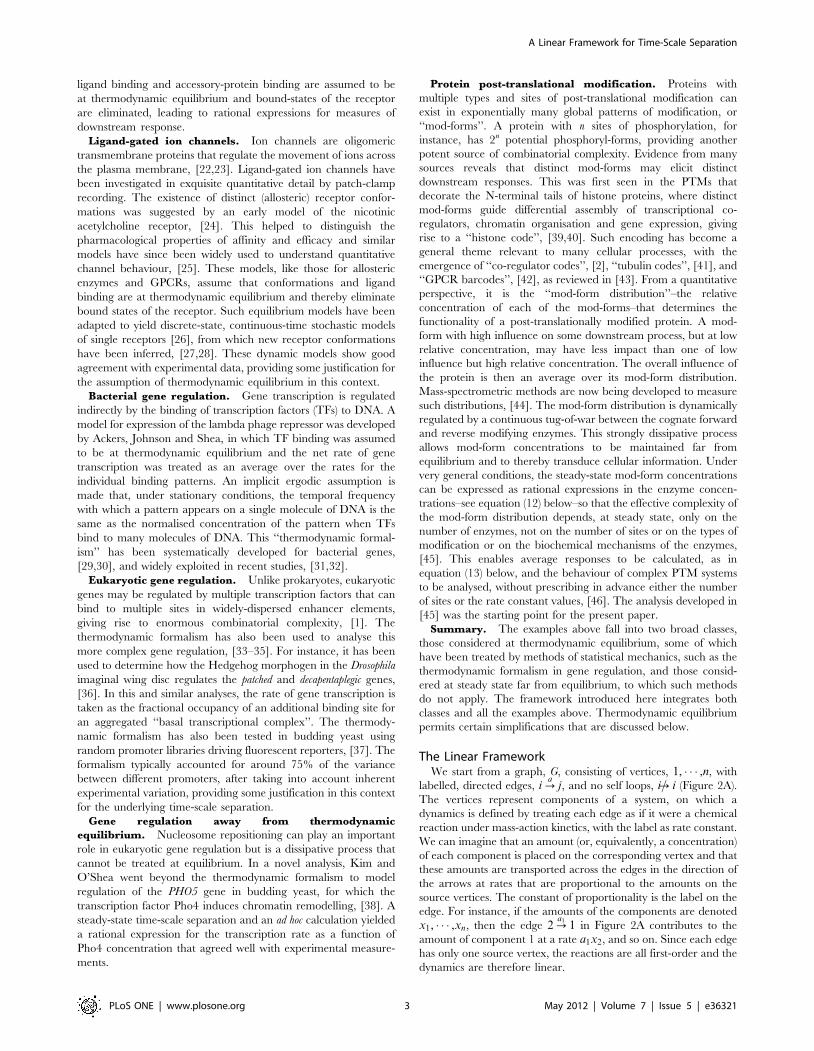
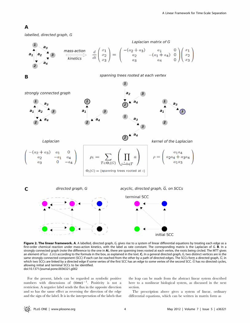
The Linear FrameworkWe start from a graph, G, consisting of vertices, 1, � � � ,n, with
labelled, directed edges, i?a
j, and no self loops, i=? i (Figure 2A).
The vertices represent components of a system, on which a
dynamics is defined by treating each edge as if it were a chemical
reaction under mass-action kinetics, with the label as rate constant.
We can imagine that an amount (or, equivalently, a concentration)
of each component is placed on the corresponding vertex and that
these amounts are transported across the edges in the direction of
the arrows at rates that are proportional to the amounts on the
source vertices. The constant of proportionality is the label on the
edge. For instance, if the amounts of the components are denoted
x1, � � � ,xn, then the edge 2?a1
1 in Figure 2A contributes to the
amount of component 1 at a rate a1x2, and so on. Since each edge
has only one source vertex, the reactions are all first-order and the
dynamics are therefore linear.
A Linear Framework for Time-Scale Separation
PLoS ONE | www.plosone.org 3 May 2012 | Volume 7 | Issue 5 | e36321
For the present, labels can be regarded as symbolic positive
numbers with dimensions of (time){1. Positivity is not a
restriction. A negative label sends the flux in the opposite direction
and so has the same effect as reversing the direction of the edge
and the sign of the label. It is in the interpretation of the labels that
the leap can be made from the abstract linear system described
here to a nonlinear biological system, as discussed in the next
section.
The prescription above gives a system of linear, ordinary
differential equations, which can be written in matrix form as
Figure 2. The linear framework. A. A labelled, directed graph, G, gives rise to a system of linear differential equations by treating each edge as afirst-order chemical reaction under mass-action kinetics, with the label as rate constant. The corresponding matrix is the Laplacian of G. B. In astrongly connected graph (note the difference to the one in A), there are spanning trees rooted at each vertex, the roots being circled. The MTT givesan element of ker L(G) according to the formula in the box, as explained in the text. C. In a general directed graph, G, two distinct vertices are in thesame strongly connected component (SCC) if each can be reached from the other by a path of directed edges. The SCCs form a directed graph, G, inwhich two SCCs are linked by a directed edge if some vertex of the first SCC has an edge to some vertex of the second SCC. G has no directed cycles,allowing initial and terminal SCCs to be identified.doi:10.1371/journal.pone.0036321.g002
A Linear Framework for Time-Scale Separation
PLoS ONE | www.plosone.org 4 May 2012 | Volume 7 | Issue 5 | e36321

dx
dt~ L (G):x , ð3Þ
where x is the column vector of component amounts and L(G) is
called the Laplacian matrix of G. Such matrices were first introduced
by Gustav Kirchhoff in his study of electrical circuits, [47]. They
resemble discretisations of the continuous Laplacian operator but
they are known in many different versions, [48]. As Laplacians
have been widely studied, the results outlined here may be known
under different guises.
Since material is neither created nor lost, the system has at least
one conservation law given by the total amount of matter,
xtot~x1z � � �zxn, which remains constant at all times. Hence,
1{: L(G)~0, where 1 is the all-ones column vector and { denotes
transpose.
If we imagine the system being started with arbitrary amounts of
each component, we expect that the dynamics will eventually relax
to a steady state. This is, indeed, true for any graph. The
dynamical behaviour of (3) has several interesting features, as well
as biological applications; for instance, to the dynamical behaviour
of ligand-gated ion channels. However, our interest here is in the
steady state, so we defer a full discussion of the dynamics to
elsewhere (I. Mirzaev, J. Gunawardena, in preparation). At steady
state, dx=dt~0, or, equivalently, x lies in the kernel of the
Laplacian, x [ ker L(G). The kernel can be determined in two
steps, first for a strongly connected graph and then for any graph.
A strongly connected graph is one in which any two distinct
vertices can be joined by a series of edges in the same direction.
The graph in Figure 2A is not strongly connected (vertex 1 cannot
be reached from vertex 3), unlike that in Figure 2B. Strong
connectivity depends only on the edge structure and not on the
labels. A key observation is that, if the graph is strongly connected,
then ker L(G) is one dimensional, [45]. No matter how many
components are present in the graph and whatever arbitrary
amounts of each component are present initially, once steady state
is reached only a single degree of freedom is left. If the steady-state
amount of any one component is known, then the steady-state
amounts of all components are mathematically determined. This
remarkable rigidity is the basis for the eliminations in all of the
examples discussed here.
To actually calculate the steady states, it is necessary to
determine a canonical basis element r [ ker L(G). This is
provided by the Matrix-Tree Theorem (MTT). Versions of this
go back to Kirchhoff, [49], but the one needed for our purposes
was first proved by Bill Tutte, one of the founders of modern graph
theory, [50]. To calculate ri, take the product of all the labels on a
spanning tree of G rooted at vertex i and add the products over all
such trees (Figure 2B, box). A spanning tree is a fundamental
concept in graph theory. It is a subgraph of G that contains each
vertex of G (spanning) which has no cycles when edge directions
are ignored (tree) and for which i is the only vertex with no
outgoing edges in the tree (rooted). The spanning trees for the
strongly-connected graph in Figure 2B are shown there along with
the calculation of r [ ker L(G). More spanning tree are shown in
Supporting Information S1.
The kernel could have been calculated by standard linear
algebraic methods using determinants. The significance of the
MTT is that it expresses ri as a polynomial in the labels with
positive coefficients (Figure 2B). The cancellations arising from the
alternating signs in a determinant are thereby resolved.
Results equivalent to the MTT have been frequently rediscov-
ered in biology, for instance, in the King-Altman procedure in
enzyme kinetics, [6], and in Terrell Hill’s thermodynamical
studies, [51], but without appreciating the broad scope of its
application.
If x is any steady-state, then, since dim ker L(G)~1, we know
that x~lr, where l [R. The undetermined l reflects the single
degree of freedom that remains at steady state. It can be removed
by normalising in different ways:
1: xi~ri
r1
� �x1 2: xi~
ri
rtot
� �xtot : ð4Þ
In 1, one of the vertices, by convention vertex 1, is chosen as a
reference. In 2, xtot plays a similar role, with rtot~r1z � � �zrn.
It follows from the MTT that the terms in brackets in (4), ri=r1
and ri=rtot, are rational expressions in the labels. The component
amounts, xi, have been eliminated in favour of these rational
expressions, along with x1 or xtot, respectively. The rational
expressions in each of the examples discussed here arise in exactly
this way.
The situation when G is not strongly connected is also of
interest. For a general graph G, the dimension of ker L(G) is
given by the number of terminal strongly connected components.
A strongly connected component (SCC) of a graph G is a maximal
strongly-connected subgraph (Figure 2C). The SCCs themselves
form a directed graph, G, in which two SCCs are linked by a
directed edge if some vertex of the first SCC has an edge to some
vertex of the second SCC. G has no directed cycles, which allows
initial and terminal SCCs to be identified. A description of
ker L(G) in terms of the terminal SCCs is given in the Appendix
of [52]. We go further here by using the MTT to give explicit
expressions for the basis elements in terms of the labels. For each
terminal SCC, t, let rt [Rn be the vector which, for vertices in that
SCC, agrees with the values coming from the MTT applied to that
SCC in isolation, while for any other vertex, j=[t, (rt)j~0. These
vectors form a basis for the kernel of the Laplacian:
ker L(G)~Sr1, � � � ,rT T , ð5Þ
where T is the number of terminal SCCs. An outline proof is
provided in Supporting Information S1.
When G is not strongly connected there is more than one steady
state, up to a scalar multiple. This should not be confused with
multistability, as there is a corresponding increase in the number
of conservation laws. Steady states may also have components with
zero amounts, even when the initial conditions do not, in contrast
to the strongly connected case, in which the MTT shows that each
component is positive at steady state. For some applications, it is
useful to know which steady state is reached from a given initial
condition. Such dynamical issues will be dealt with elsewhere (I.
Mirzaev, J. Gunawardena, in preparation).
We discuss some additional general results later but turn next to
explaining how such a linear framework can be applied to
nonlinear biological systems.
The Uncoupling ConditionThe leap from linearity to nonlinearity can be made in one of
two ways. For time-scale separation, as in the examples discussed
above, nonlinearity is encoded in the labels. Up till now, the labels
have been treated as uninterpreted symbols. In any application the
labels arise from the biochemical details of the system being
studied. A label may be an arbitrary rational expression involving
rate constants of actual chemical reactions or concentrations of
actual chemical species. For instance, the following expression for
a label would be legitimate
A Linear Framework for Time-Scale Separation
PLoS ONE | www.plosone.org 5 May 2012 | Volume 7 | Issue 5 | e36321

a~(k1½X1�zk2½X2�)½X3�
(k3zk4)½X4�,
where k1, � � � ,k4 are rate constants and X1, � � � ,X4 are chemical
species. In our experience, so far, labels have been polynomials in
the concentrations with coefficients that are rational in the rate
constants. However, there is no mathematical reason to exclude
more complex expressions, like the one above. The crucial
restriction, which we refer to as the uncoupling condition, is that if a
concentration, [X], appears in a label, then the species X must not
correspond to a vertex in the graph. It could, however, correspond
to a slow component in a time-scale separation, which is often how
such a label arises. The uncoupling condition is essential to
preserve linearity but it can be circumvented in some cases, as
explained below. The other encoding of nonlinearity will be
discussed later.
The key to applying the framework in a time-scale separation is,
first, to find a directed graph whose components represent the fast
variables in the sub-system, which has a labelling that satisfies the
uncoupling condition, and, second, to show that the steady states
of the linear Laplacian dynamics coincide with those of the full
nonlinear biochemical dynamics of the sub-system. It is crucial to
note that only the steady states need coincide, not the transient
dynamics. If the latter were the same, then the sub-system would
itself be linear, which is not the case in any of the applications. In
this way, dynamical nonlinearity with simple rate constants is
traded for dynamical linearity with complex labels. The trade-off is
highly beneficial, as it allows the steady states of the nonlinear sub-
system to be algorithmically calculated without knowing in
advance the values of any rate constants. This enables the internal
complexity of the fast components to be eliminated, giving rise to
rational expressions based on one or the other of the normalisa-
tions in (4). This procedure underlies all the examples discussed
here. We turn now to outlining how the framework is used in these
applications.
Applications Far from EquilibriumEnzyme kinetics. As a simple demonstration of the frame-
work, we return to the Michaelis-Menten example in the
Introduction. More complex enzymes are treated in essentially
the same way.
We first rewrite the reaction scheme in (1) after annotating the
reactions with their corresponding rate constants:
SzE ES ?k3
PzE ð6Þ
The labelled, directed graph is constructed following the time-scale
separation described in the Introduction. The vertices correspond
to the fast components, which are the enzyme states E and ES.
The edges amalgamate the effects of the reactions in which these
components are involved. Edges outgoing from vertex E absorb
the concentrations of slow components (in this case S), while all
other edges only have rate constants in their labels. The following
graph emerges
E /{{{{{{{{{{?
k1½S�
k2 z k3
ES ð7Þ
in which the vertices have been annotated for convenience with
the names of the corresponding components. [S] is the only
concentration that appears in a label and it is not the
concentration of a vertex in the graph. The uncoupling condition
is therefore satisfied.
It is not difficult to check that, with this labelling, the steady
states of the Laplacian dynamics given by (3) are the same as the
steady states of the fast components given by the actual
biochemical reactions in (6).
Graphs constructed like (7), even for more complex enzymes,
are naturally strongly connected because bound states of the
enzyme usually release the enzyme eventually. (If there are dead-
end complexes, they must be formed reversibly, thereby also
ensuring strong connectivity.) Accordingly, the MTT can be
applied and it follows from the formula in Figure 2B that
rE~k2zk3 , rES~k1½S� : ð8Þ
If the system is assumed to be at a steady state, then it follows from
the second elimination formula in (4) that
½ES �~ rES
rtot
� �Etot
where Etot~½E�z½ES � is the total concentration of enzyme and
rtot~rEzrES . Note how [ES] has been eliminated in favour of
Etot and the expressions appearing in r, which come from the
MTT. The enzyme rate can now be calculated as
d½P�dt
~k3½ES �~ k3Etot½S�(k2zk3)=k1z½S�
,
and the Michaelis-Menten formula in (2) emerges with the usual
aggregated parameters, [8],
Vmax~k3Etot , KM~k2zk3
k1: ð9Þ
King and Altman were the first to formalise this kind of algebra for
more complex enzymes, [6]. They did not use graph theory and
spanning trees but introduced ‘‘reaction patterns’’, a terminology
that has persisted in the biochemical literature, [8]. The King-
Altman procedure is equivalent to the MTT.
Post-translational modification. The advantage of using
the framework introduced here becomes particularly clear when
moving from the behaviour of a single enzyme to that of a network
of enzymes in post-translational modification. The identical
mathematical machinery can be used in this quite different
context. This was first described in [45] but we clarify here several
issues whose significance was only understood more recently.
Consider a substrate, S, that is subject to different types of PTM
(phosphorylation, methylation, acetylation, etc), with each mod-
ification potentially taking place at many sites. (There may be
multiple such substrates but we consider only one for simplicity
here.) We will analyse such a substrate under the assumption that
it, and the enzymes acting upon it, are at steady state. The
substrate S may have many mod-forms, which can be enumerated,
S1, � � � ,SN . The number of mod-forms, N, typically depends
exponentially on the number of sites, although, with modifications
like methylation or ubiquitination, the detailed combinatorics may
be more complicated, [43]. There is a natural directed graph on
the vertices 1, � � � ,N, in which there is an edge i?j if some
A Linear Framework for Time-Scale Separation
PLoS ONE | www.plosone.org 6 May 2012 | Volume 7 | Issue 5 | e36321
k2
'k1

enzyme (and there may be several) is capable of converting Si to Sj.
Note that enzymes may be processive and able to make several
modifications in one encounter between enzyme and substrate, so
that an individual enzyme may be implicated in many edges with
Si as the source vertex. It is an empirical observation that each
individual transformation from Si to Sj can generally be undone, if
not directly, then through intermediate mod-forms. Hence, Si can
be recovered, eventually, from Sj, so that the directed graph is
naturally strongly connected.
This is an obvious setting to apply the linear framework. A
labelling of the edges is needed that captures the underlying
biochemistry and also satisfies the uncoupling condition. PTMs fall
naturally into two biochemical classes: those based on small-
molecule modifications (phosphorylation, methylation, acetylation,
etc) in which the donor molecules are regenerated by core
metabolism and modification is undertaken by a single enzyme;
and those based on polypeptide modifications (ubiquitin, SUMO,
NEDD, etc) in which the donor molecules are synthesised by gene
transcription and modification requires a series of enzymes, [43].
It is easiest to focus on the first class of small-molecule
modifications; analysis of the second class is still work in progress.
With small-molecule modifications, the biochemistry of modi-
fication is significantly different from that of demodification, since
the former involves the donor molecule that brings the modifying
group, while the latter is a hydrolysis. Such details have been
usually disregarded in the literature, where it has been the custom
to treat all enzymes as if they followed the Michaelis-Menten
scheme in (1). This overlooks much of the biochemical knowledge
that has accumulated since 1913, [53]. Reaction mechanisms for
kinases and phosphatases have been analysed, [54,55], although
less is known about the enzymology of other PTMs. One of the
virtues of the linear framework is that it shows how realistic
enzyme mechanisms can be analysed, thereby helping to bridge
the gap between enzyme biochemistry and systems biology, [56].
By making appropriate assumptions regarding the core biochem-
ical machinery that maintains the modifying groups, the modifi-
cation and demodification enzymes may be assumed to follow
mechanisms built up from just three basic reactions: creation of an
intermediate complex; break-up of an intermediate complex; and
conversion of one intermediate complex to another
EzS�?Y� , Y�?EzS� , Y�?Y� : ð10Þ
Here, the intermediate complexes have been denoted Y�, and the
asterisk in S� or Y� can be any index in the list of substrate forms
or intermediate complexes, respectively. This scheme allows for
complex enzyme mechanisms that may have multiple intermedi-
ates, yield multiple products, exhibit arbitrary degrees of
processivity and be fully reversible. Enzymes may also use different
mechanisms for different mod-forms. While (10) is quite general, it
does impose some restrictions on enzyme mechanisms, as
discussed further in [56], although these do not seem to be
restrictive for most metabolic PTMs.
If the enzyme E is able to convert Si to Sj by some mechanism
built up from (10), then the linear framework may be applied to
the enzyme intermediates just as described previously for enzyme
kinetics. The intermediate complexes can be eliminated at steady
state and the rate of conversion from Si to Sj can be calculated as
aE ½Si�½E�, where aE is a (possibly very complicated) rational
expression in the rate constants of the mechanism. For instance, if
the conversion from Si to Sj takes place by the Michaelis-Menten
scheme in (6), then it follows from (8) by using the first elimination
formula in (4) that the conversion rate is given by
k3
KM
� �½S�½E� :
In this case, aE~k3=KM . What the linear framework shows is that
a similar formula holds for any reaction scheme built up from (10),
no matter how complicated.
The key point is that such formulas are linear in [Si], which
means that aE ½E� can be incorporated into a label in the mod-form
graph. If several enzymes are able to convert Si to Sj, each
contributes additively to the rate, and the edge from Si to Sj can be
labelled
XE
aE ½E� : ð11Þ
The concentrations in such labels are those of enzymes. It follows
that the uncoupling condition will be satisfied so long as enzymes
are not also substrates. We assume this, for the moment, but
explain below how it can be circumvented. With this labelling, it
can be shown that the steady states of the Laplacian dynamics in
(3) are identical with the steady states of the nonlinear dynamics
coming from the specified enzyme mechanisms. This holds for
arbitrary numbers of sites, arbitrary numbers of modifying and
demodifying enzymes and arbitrary reaction mechanisms built up
from those in (10), [45]. The MTT can now be applied to show
that the substrate forms can be eliminated at steady state. The
relative concentration of each mod-form, Si, can be explicitly
written down using the second normalisation in (4),
½Si�Stot
~ri(½E1�, � � � ,½Ep�)X
u
ru(½E1�, � � � ,½Ep�): ð12Þ
We assume here that there are p forward and reverse enzymes in
total, E1, � � � ,Ep. The ri are given by the MTT as polynomials in
the free-enzyme concentrations, through the labels described by
(11). We see from (12) that the exponential complexity arising from
combinatorial patterns of modification disappears at steady state:
the effective (algebraic) complexity at steady state depends only on
the number of enzymes, not on the number of sites. As we have
seen, this surprising conclusion is a consequence of the strong
connectivity of the mod-form graph.
In this example, the elimination process is hierarchical. The
enzyme-bound intermediate complexes are first eliminated in
favour of the mod-forms and the free enzymes, yielding the labels
for the mod-form graph, and the mod-forms are then eliminated
to leave only the free enzymes.
As discussed above, different mod-forms may elicit different
downstream responses. The expression in (12) can be thought of as
the steady-state probability of finding the substrate in mod-form Si.
If Si elicits a quantitative level of effect given by ai, then the overall
response of the PTM substrate can be estimated as an average
over this probability distribution,
Xi
ai½Si�Stot
� �: ð13Þ
It is assumed here, as part of the time-scale separation depicted in
Figure 1, that the downstream response is operating sufficiently
slowly to average over the different mod-forms. This is similar to
the calculation of the rate of gene expression as a function of
transcription factor concentrations (Figure 3A). In the case of
A Linear Framework for Time-Scale Separation
PLoS ONE | www.plosone.org 7 May 2012 | Volume 7 | Issue 5 | e36321
PTM, formulas like (13) are functions of free enzyme concentra-
tions, which are set by the enzyme mechanisms and cannot be
readily estimated or approximated. However, since enzymes are
assumed to be neither synthesised nor degraded (see below for how
this restriction can be addressed), there is a conservation law for
each enzyme. These may be explicitly written down in terms of the
symbolic rate constants,
E1,tot ~ w1(½E1�, � � � ,½Ep�)
..
. ... ..
.
Ep,tot ~ wp(½E1�, � � � ,½Ep�)ð14Þ
to give p nonlinear algebraic equations for the p unknown free-
enzyme concentrations. The essential nonlinearity in the bio-
chemistry makes its appearance in these equations. For instance,
for given total amounts of enzymes and substrate, there may be
multiple solutions to (14), giving rise to multistability, [46,57].
Equations (12) and (14) together provide a complete mathematical
description of the substrate’s behaviour at steady state.
For PTM, the uncoupling condition has significant consequenc-
es, as it appears to rule out enzyme cascades, such as the MAP
kinase cascade, in which the substrate at one level becomes the
enzyme for the next. However, in this case, substrate-forms at
distinct levels of the cascade can never be inter-converted and so
appear in distinct connected components of the graph. If the
concentration appearing in a label is that of a component in a
different connected component, then, under suitable conditions,
the analysis can still be undertaken in a recursive manner. Feliu
et al work out the case of a linear cascade, [58], but the general
conditions under which this method can be exploited have not yet
been determined.
Ligand Binding, at Equilibrium and BeyondSeveral examples discussed above involve the binding of ligands
to various kinds of ‘‘scaffolds’’. These examples have usually been
treated by assuming that the ligands and the scaffolds are at
thermodynamic equilibrium. The case of the PHO5 gene in yeast,
discussed above, makes clear that a more general treatment is
necessary. The linear framework is not limited to systems at
equilibrium. We first describe how it can be used in sufficient
generality to allow for dissipative behaviour and then discuss the
simplifications that arise at equilibrium.
Consider a scaffold, S, that may correspond to an allosteric
protein, receptor, ion channel, DNA segment, chromatin, etc. The
scaffold can exist in multiple states, S1, � � � ,Sm, corresponding to
protein conformations, states of binding of accessory proteins,
states of DNA looping, patterns of nucleosome organisation, etc.
The number of scaffold states need not be high; in the Monod-
Wyman-Changeux model of allostery, for instance, m is often two,
corresponding to a ‘‘relaxed’’ and a ‘‘tense’’ state (Figure 3B). The
corresponding state transitions may take place at equilibrium, as in
allosteric transitions, or require energy expenditure and be
dissipative, as in nucleosome reorganisation. Ligands may bind
to multiple sites on the scaffold in each of its states, with
overlapping site preferences and cooperativity. To avoid excessive
notation, we discuss here the case in which distinct ligands do not
compete for sites, so that each site is associated with a specified
ligand, which may or may not be bound there. In this case, the
pattern of ligand binding can be encoded by a bitstring, b1, � � � ,bn,
where n is the number of sites and bi~0 indicates that site i is
empty, while bi~1 indicates that site i is bound by its cognate
ligand. (A more complicated encoding is needed when distinct
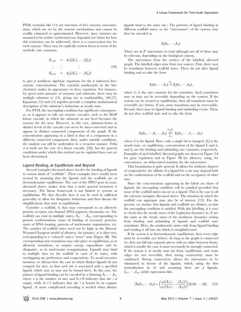
ligands bind to the same site.) The patterns of ligand binding in
different scaffold states, or the ‘‘microstates’’ of the system, may
then be encoded as
Si(b1, � � � ,bn) :
There are m:2n microstates in total although not all of these may
be relevant, depending on the biological context.
The microstates form the vertices of the labelled, directed
graph. The labelled edges arise from two sources. First, there may
be transitions between scaffold states. These do not alter ligand
binding and so take the form
Si(b1, � � � ,bn)?k1
Sj(b1, � � � ,bn) ,
where k1 is the rate constant for the transition. Such transitions
may or may not be reversible depending on the context. If the
system can be treated at equilibrium, then all transitions must be
reversible (see below). If not, some transitions may be irreversible.
Second, there may be ligand binding and unbinding events. These
do not alter scaffold state and so take the form
Si(b1, � � � ,0, � � � ,bn)k3
'k
2½L�
Si(b1, � � � ,1, � � � ,bn)
where L is the ligand. Here, only a single bit is changed. [L] is the
steady-state, or equilibrium, concentration of the ligand L and k2
and k3 are the binding and unbinding rate constants, respectively.
Examples of such labelled, directed graphs are shown in Figure 3A
for gene regulation and in Figure B for allostery, using, for
convenience, an abbreviated notation for the microstates.
This formulation is quite general. It allows for arbitrary degrees
of cooperativity: the affinity of a ligand for a site may depend both
on the conformation of the scaffold and on the occupancy of other
sites.
Since the concentrations appearing in the labels are those of
ligands, the uncoupling condition will be satisfied provided that
none of the scaffold states can act as a ligand. This is the case in all
the relevant examples discussed above. The situation in which the
scaffold can aggregate may also be of interest, [12]. For the
present, we assume that ligands and scaffolds are distinct, so that
the uncoupling condition is satisfied. With this labelling, it is easy
to check that the steady states of the Laplacian dynamics in (3) are
the same as the steady states of the nonlinear dynamics arising
from binding and unbinding of ligands and scaffold state
transitions. Here, the nonlinearity arises only from ligand binding
and trading it off into the labels is straightforward.
If the system is at thermodynamic equilibrium, then every edge
must be reversible (see below). As long as the graph is connected
(ie: does not fall into separate pieces with no edges between them),
which is usually the case, it must necessarily be strongly connected.
If the system is at steady state far from equilibrium, and some
edges are not reversible, then strong connectivity must be
confirmed. Strong connectivity allows the microstates to be
eliminated in favour of the ligands, which, using the first
normalisation in (4) and assuming there are p ligands,
L1, � � � ,Lp, yields expressions like.
½Si(b1, � � � ,bn)�~ ri(½L1�, � � � ,½Lp�)r1(½L1�, � � � ,½Lp�)
� �½S1(0, � � � ,0)� : ð15Þ
A Linear Framework for Time-Scale Separation
PLoS ONE | www.plosone.org 8 May 2012 | Volume 7 | Issue 5 | e36321
3
Here, the reference microstate is taken to the be one in which no
ligands are bound, which is helpful for calculating fractional
saturation, as explained in Supporting Information S1. The
second normalisation in (4) is more suitable for calculating rates of
gene expression, following the method used previously for PTM.
As with PTM, the free-ligand concentrations are determined by
p conservation laws for the p ligands, similar to those in (14).
However, it is often assumed that ligands are in substantial excess
over scaffolds, so that, to a first approximation, ½Li�&Li,tot. If this
is not the case, then the p nonlinear equations must be solved to
determine the actual free-ligand concentrations.
Strong connectivity is not mentioned in the dissipative analysis
of PHO5, [38]. The corresponding gene regulation function was
calculated by Matlab from the steady-state equations. In this
example, the directed graph is essentially identical to that shown in
Figure 4b of [38], which is easily checked to be strongly connected
despite its irreversible edges. As we have seen, it is the strong
connectivity that is essential for eliminating the microstates and
calculating the gene-regulation function.
An important special case of the framework arises when the
system is at thermodynamic equilibrium. In this case, the principle
of detailed balance (DB) provides a simpler alternative to the
MTT. The origins of this principle are discussed further in the
next section. DB states that a chemical reaction at equilibrium is
always reversible and that any pair of such reversible reactions is
independently at equilibrium, irrespective of any other reactions in
which the substrates or products participate. To see the
implications for the labelled, directed graph constructed above,
it is convenient to enumerate the microstates, as we did earlier
when explaining the graphical framework, using the numbers
Figure 3. Ligand binding. A. Gene regulation, with two transcription factors (TFs), L1 and L2, binding to a promoter. A labelled, directed graph canbe constructed as described in the text, with the microstates being denoted here by the bitstrings 00, � � � ,11. In this example there are no changes ofconformational state in the scaffold, as would be the case if there was DNA looping or displacement of nucleosomes. The rate of mRNA transcriptionby RNA polymerase (RNAP) is assumed to depend on the pattern of TF binding as shown and the overall rate is calculated as an average over theprobabilities of finding the promoter in each of the patterns. Assuming the system is at an equilibrium, x, these probabilities are given by the ratios,x00=xtot, � � � ,x11=xtot, which can be calculated using the second elimination formula in (4). B. An allosteric homodimeric protein is shown in twoconformational states, relaxed (R) and tense (T). The labelled, directed graph has both conformational state changes in the scaffold as well as ligandbinding and unbinding. The microstates are denoted here R001, � � �R11,T00, � � � ,T11. Labels have been omitted for clarity. For allosteric enzymes,the overall rate of product formation is usually assumed to be proportional to the fraction of sites that are bound by ligand (fractional saturation), asshown. This can be calculated as described in Supporting Information S1.doi:10.1371/journal.pone.0036321.g003
A Linear Framework for Time-Scale Separation
PLoS ONE | www.plosone.org 9 May 2012 | Volume 7 | Issue 5 | e36321
1,2,3, � � � for the vertices and omitting the details of conformation
and ligand binding. We assume the graph is strongly connected.
DB implies that any edge j ?a
i is reversible. Given any pair of
reversible edges,
jb'a
i ð16Þ
and an equilibrium state x, DB implies that xi~(a=b)xj ,
irrespective of any other edges impinging on i or j. The quantity
(a=b) is an equilibrium constant.
DB makes it easy to calculate the equilibrium state, x. Choose a
reference vertex, 1, which we assume to be a microstate in which
no ligands are bound, such as 1~S1(0, � � � ,0). Given any other
vertex i, choose a path of reversible edges from 1 to i,
1b1
'a1
j1b2
'a2
� � �bk{1
'ak{1
jk{1bk
'ak
i
Such a path must always exist because of strong connectivity. It
then follows that
xi~ak
bk
� �ak{1
bk{1
� �� � � a2
b2
� �a1
b1
� �x1 : ð17Þ
This should be compared to (15) above. The product of
equilibrium constants along the path corresponds to ri=r1. As
before, this quantity is a rational expression in the labels but, now,
the numerator and denominator consist only of the single
monomials, ak � � � a1 and bk � � � b1, respectively. At equilibrium,
DB cuts down the rooted trees of the MTT to a single path from 1.
Of course, there may be many such paths. However, the rate
constants are not free to vary arbitrarily. DB requires that formula
(17) gives the same result no matter which path is taken from 1 to i.
This constraint may be summarised in the ‘‘cycle condition’’: for
any cycle of reversible edges, the product of the rate constants on
clockwise edges equals the product on counterclockwise edges
(Figure 3A). This condition is necessary and sufficient for (17) to be
independent of the path taken and for every equilibrium state of
the graph to satisfy DB; the proof is given in Supporting
Information S1.
The so-called ‘‘thermodynamic formalism’’ has often been used
to analyse systems at equilibrium, [59,60], particularly in the
context of gene regulation, [30,35,61]. The equilibrium state is
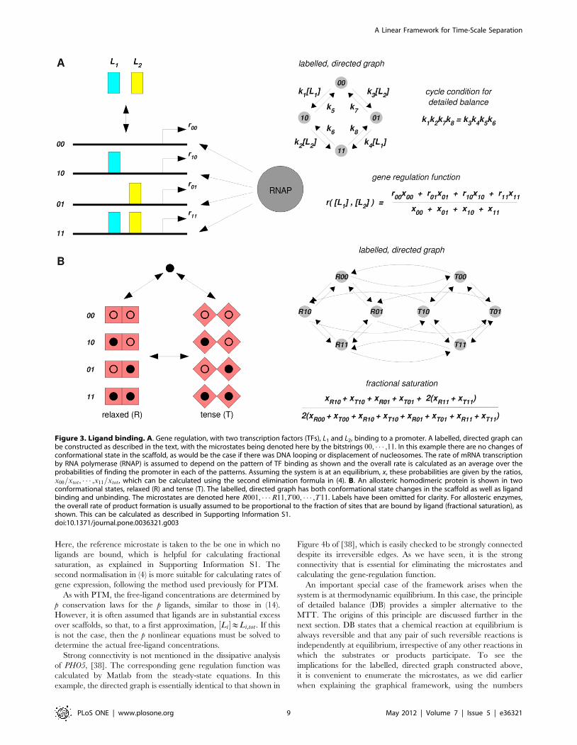
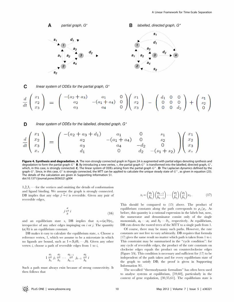
Figure 4. Synthesis and degradation. A. The non-strongly connected graph in Figure A is augmented with partial edges denoting synthesis anddegradation to form the partial graph Gz B. By introducing a new vertex, �, the partial graph Gz is transformed into the labelled, directed graph, G� ,which, in this case, is strongly connected. C. The linear system of ODEs arising from the partial graph Gz. D. The Laplacian dynamics defined by thegraph G� . Since, in this case, G� is strongly connected, the MTT can be applied to calculate the unique steady state of Gz, as given in equation (23).The details of the calculation are given in Supporting Information S1.doi:10.1371/journal.pone.0036321.g004
A Linear Framework for Time-Scale Separation
PLoS ONE | www.plosone.org 10 May 2012 | Volume 7 | Issue 5 | e36321
2

calculated as a sum of interaction energies. The relationship
between this and the linear framework comes through van’t Hoff’s
formula for the equilibrium constant, which may be written, for
the reversible edge (16),
lna
b
� �~
DU
RT: ð18Þ
Here, DU is the difference in Gibbs free energy between
microstate i and microstate j, R is the gas constant (ie: the molar
Boltzmann constant) and T is the absolute temperature. Formula
(18) allows the multiplicative formulation of the linear framework
in (17) to be converted to the additive formulation favoured in
thermodynamics
RT lnxi
x1
� �~{DU1{ � � �{DUk :
In gene regulation studies, the interaction energies have usually
been limited to those of transcription factors binding to DNA and
of transcription factors binding to each other when they are
nearest neighbours or otherwise able to interact physically,
[35,37]. However, both the thermodynamic formalism and the
linear framework can incorporate higher-order interactions and
cooperativities as needed.
The thermodynamic formalism and the linear framework are
equivalent for systems at thermodynamic equilibrium and related
to each other as just explained. The linear framework comes into
its own for analysing systems far from equilibrium and is well
suited to the modern programme of unravelling complex
eukaryotic gene regulation functions, [62].
Chemical Reaction Network Theory (CRNT)We mentioned previously that the linear framework can encode
nonlinearity in two ways and we have discussed at length the first
way, through the labels. Here, we briefly discuss the second way,
through the vertices, which arises in CRNT. In this case, the
framework is not associated with a time-scale separation but
CRNT is often used to determine steady-state properties.
CRNT originates in Horn and Jackson’s pioneering attempt to
extend thermodynamic reasoning from equilibrium to far-from-
equilibrium systems, [63]. If we have a reversible chemical
reaction, such as
k2
'k1
then mass-action kinetics implies that the ratio of the equilibrium
concentrations is independent of the starting conditions of the
reaction and depends only the rate constants,
½B�½A�~
k1
k2: ð19Þ
A similar relationship holds generally for any chemical reaction at
equilibrium. Such formulas can also be deduced directly from
equilibrium thermodynamics, without making kinetic assumptions
about the rates of reactions, [64]. For an isolated reaction such as
this, kinetics is consistent with thermodynamics. However, a
network of chemical reactions may have kinetic equilibria that do
not satisfy thermodynamic constraints. Gilbert Lewis sought to
avoid such paradoxes by suggesting the principle of detailed
balance (DB), as stated in the previous section, [65]. It was later
realised that DB is a consequence of the fundamental time-
reversibility of microscopic processes, whether classical or quan-
tum, [66,67].
Horn and Jackson sought to extend thermodynamic properties
like (19) to steady states far from equilibrium, [63]. Under mass-
action kinetics, any network of chemical reactions gives rise to a
system of nonlinear ordinary differential equations, dx=dt~f (x),for the concentrations, x1, � � � ,xm of the various chemical species.
Here, the nonlinear function f : Rn?Rn defines the dynamics on
the species level. To disentangle the nonlinearities, the stoichio-
metric expressions that appear on either side of a reaction were
treated as new entities called ‘‘complexes’’. A hypothetical reaction
such as Az2B?3C gives rise to the two complexes, Az2B and
3C. Each reaction defines a directed edge between complexes and
the mass-action rate constant provides the edge with a label. Any
network of chemical reactions, N, thereby gives rise to a labelled,
directed graph, GN. The number of vertices in GN is the number of
distinct complexes, m, among all the reactions in the network.
The Laplacian matrix of this graph defines a linear function,
L(GN ) : Rm?Rm, at the complex level that is the analogue of the
nonlinear f : Rn?Rn at the species level. The relationship
between f and L(Gn) is expressed in the fundamental equation.
f (x)~Y : L(GN ):Y(x) , ð20Þ
where Y : Rm?Rn is a linear function that records the
stoichiometry of each species in a complex and Y : Rn?Rm is a
nonlinear function that records the mass-action monomial
corresponding to each complex, [63]. The ‘‘dot’’ signifies
composition of functions. Horn and Jackson were unaware at
the time of the Laplacian interpretation, which was first pointed
out in [68]. The decomposition in (20) is the starting point of
CRNT, which was subsequently developed by Feinberg and his
students, [69,70]. The decomposition leads to Horn and Jackson’s
concept of a ‘‘complex-balanced’’ steady state, x, for which
L(GN ):Y(x)~0. This may be reached far from equilibrium but
still satisfies properties to be expected at equilibrium, including
relationships between concentrations and rate constants that
generalise (19), [63].
Synthesis and DegradationA common feature of all the examples discussed previously is
that synthesis and degradation were entirely ignored, although
they are often significant in the biological context. It is an
indication of the power of the linear framework that it can be
readily extended to accommodate this.
Consider, as before, a labelled, directed graph, G, on vertices
1, � � � ,n but now allow each vertex in this ‘‘core graph’’ to have
additional partial labelled edges,
?si
i or i?di
corresponding to zero-order synthesis or first-order degradation,
respectively (Figure 4A). Each vertex may have any combination
of synthesis and degradation, including neither or both. Call this
‘‘partial graph’’ Gz. As before, there is a linear dynamics on Gz,
which may be described by the system of differential equations
dx
dt~ L (G):x{D:xzS , ð21Þ
A Linear Framework for Time-Scale Separation
PLoS ONE | www.plosone.org 11 May 2012 | Volume 7 | Issue 5 | e36321
BA
where L(G) is the Laplacian matrix of the core graph, G. Here, Dis a diagonal matrix with Dii~di and S is a column vector with
Si~si, using the convention that di or si is zero if the
corresponding partial edge at vertex i is absent.
The dynamics defined by (21) has several different features to
that described by (3). It is easy to construct examples in which
degradation cannot keep up with synthesis, so that a component
becomes infinite and undefined. This usually arises from an error
in formulating the model. Conversely, if synthesis cannot keep up
with degradation, a component may become zero, which may not
be an error. What is required, is to determine whether any
components become infinite at steady state and, if not, to
determine the steady-state values of the components in terms of
the labels.
Elimination also takes a different form in (21) because it is non-
homogeneous: if x is a steady state of (21), it does not follow that lx
is also a steady state. Indeed, the single degree of freedom that is
found in a strongly-connected graph at steady state is no longer
present in the partial graph, as the total amount of matter in the
system is no longer conserved. Irrespective of how much matter is
present initially, it is the rates at which matter enters and leaves the
system that determine the final distribution of amounts, if a steady
state is reached. This requirement is expressed in a constraint on
the steady state. Setting dx=dt~0 in (21) and using the fact that
1{: L(G)~0 in the core graph, we see that
d1x1z � � �zdnxn~s1z � � �zsn : ð22Þ
This reflects the fact that synthesis and degradation must be in
overall balance if Gz is to have a steady state.
To determine the values of the steady state, construct a labelled,
directed graph G� by adding a new vertex � to G (Figure 4B). For
each of the partial edges above, introduce into G� the edges
�?si
i or i?di � ,
respectively. G� is a proper labelled, directed graph, whose
Laplacian dynamics are governed by (3). This graph enables a
complete solution to the problem raised above. We focus on the
case that is most relevant to the applications by assuming that G� is
strongly connected. This will be the case if the core graph G is
strongly connected and there is at least one synthesis edge and one
degradation edge. However, G� may be strongly connected even
when G is not (Figure 4A, B), so that this analysis applies to a wider
class of graphs than previously.
If G� is strongly connected, then the MTT provides a basis
element for the kernel of the Laplacian, rG�[ker L(G�). We have
annotated G� to emphasise that it is quite
different from the corresponding basis element, rG , if the core
graph also happens to be strongly connected. When G� is strongly
connected, no components of the partial graph Gz become
infinite and Gz has a unique steady state x given by
xi~rG�
i
rG��: ð23Þ
Here, all the vertices of Gz have positive amounts at steady state.
The single degree of freedom in G� has been used in (23) to ensure
that x�~1. It can easily be checked that (x1, � � � ,xn,1) is a steady
state of G� if, and only if, (x1, � � � ,xn) is a steady state of Gz. The
condition for vertex � to be at steady state in G� with x�~1
corresponds exactly to equation (22) for synthesis and degradation
to be in balance in Gz.
Equation (23) shows how synthesis and degradation can be
readily accommodated within the linear framework. It may be
used to revisit all the examples discussed previously to understand
the impact of synthesis and degradation. It also opens up for
analysis a range of new biological examples. For instance,
regulated degradation is a key mechanism in the Wnt/beta-
catenin and death-receptor signalling pathways, [71–73]. Analysis
of these using the linear framework is work in progress.
Discussion
We have shown that a simple, linear, graph-theoretic frame-
work integrates time-scale separation analysis across many
different biological areas. An expert in one of these application
areas might say that we have not added anything new to that
particular area. The expert would have a point. However, the
literature suggests that experts in different areas are apparently
unaware that they are all doing the same thing. The aim of this
paper has been to reveal this shared framework and to clarify its
essentials. The neutral mathematical language adopted here–
graphs, spanning trees, strong-connectivity–is spoken more widely
than the dialect adopted in any particular area, allowing a broader
community access to the ideas. The key insight of the paper is that
elimination of internal complexity is a linear procedure that works because the
underlying graph is strongly connected. To the best of our knowledge, this
has not been articulated previously nor has it been made evident
how broadly this idea can be applied.
We believe significant advantages accrue from using such a
framework. First, as mentioned, it helps break down the barriers
between areas: a technique developed in one area may be
exploited in many others. Second, the framework reveals the
simplicity that is obscured by contextual details. Third, the
quantitative analysis of biochemical systems acquires a foundation,
instead of appearing as a series of ad hoc calculations. Fourth, such
a foundation permits new kinds of analysis, such as incorporating
synthesis and degradation, that can now be used wherever the
framework can be applied.
The framework not only unifies, it also suggests new problems to
explore. An intriguing question is whether the dynamical
behaviour of a sub-system retains any vestige of the elimination
that becomes feasible at steady state. When a graph is strongly
connected, the many degrees of freedom that are present at the
start of the dynamics (equivalent to the number of vertices in the
graph) collapse to a single-degree of freedom at steady state. But
how does this collapse come about over time? Do the degrees of
freedom gradually ‘‘condense’’? If so, what does this process of
condensation reveal about the architecture of the graph? It is well
known that transient dynamics, prior to reaching steady state, are
informative about rate constants but it is conceivable that the way
in which degrees of freedom are lost may also tell us about the
structure of the graph and, thereby, about the structure of the
underlying network of biochemical reactions.
Time-scale separation is often used to simplify the dynamics of
the slow components. In the Michaelis-Menten example, for
instance, the differential equation in (2) is a simplified description
of the system’s behaviour, in terms of the slow components only.
The method of ‘‘singular perturbation’’ provides a systematic way
to determine the quality of this approximation and to understand
how it depends on the separation between the time scales, [74].
This has been undertaken for the Michaelis-Menten reaction
mechanism, [75,76], but, surprisingly, it appears not to have been
investigated further in enzyme kinetics and not at all in other
A Linear Framework for Time-Scale Separation
PLoS ONE | www.plosone.org 12 May 2012 | Volume 7 | Issue 5 | e36321
r with the superscript
biological areas. The linear framework provides the starting point
from which to apply singular perturbation. The key to doing so is
to identify one or more non-dimensional parameters, which
become small when the time-scales are separated, [77], from
which the accuracy of the simplified dynamics can be systemat-
ically determined. If such an analysis can be undertaken in
generality, then we would have a powerful new tool for simplifying
and approximating the dynamical behaviour of complex bio-
chemical systems.
What emerges from this may be a new approach for dealing
with molecular complexity. The examples discussed here, espe-
cially gene regulation and post-translational modification, are
combinatorial mechanisms with the potential for creating astro-
nomical numbers of internal cellular states. Making sense of this
combinatorial explosion remains one of the most significant and
intractable challenges facing integrative systems biology. It
presents particular difficulties for computational methods based
on numerical simulation because they require prior specification of
all the details of the system, including the number of sites of
modification or binding, as well as the values of all rate constants.
This has made it hard to distil general principles–those that hold
irrespective of such details. The framework introduced here, in
contrast, allows these details to be treated symbolically and
mathematically, no matter how many components are present.
Details, such as the number of modification or binding sites, may
be treated as variables, without having to give them numerical
values, [46]. A new kind of analysis becomes feasible which may
have the potential to rise above the combinatorial explosion.
Methods
The conclusions were reached by mathematical analysis, for
which further details are provided in Supporting Information S1.
Supporting Information
Supporting Information S1 Additional mathematicaldetails. 1 ‘‘Kernel of the Laplacian for a general graph’’; 2
‘‘Ligand binding at thermodynamic equilibrium’’; 3 ‘‘Synthesis
and degradation’’; and the figure ‘‘Spanning trees for the labelled
directed graph in Paper Figure 4B’’.
(PDF)
Author Contributions
Wrote the paper: JG. Worked out the mathematical theory: JG.
References
1. Davidson EH (2006) The Regulatory Genome: Gene Regulatory Networks in
Development and Evolution. Academic Press.
2. Lonard DM, O’Malley BW (2007) Nuclear receptor coregulators: judges, juries
and executioners of cellular regulation. Mol Cell 27: 691–700.
3. Michaelis L, Menten M (1913) Die kinetik der Invertinwirkung. Biochem Z 49:
333–69.
4. Gunawardena J (2012) Some lessons about models from Michaelis and Menten.
Mol Biol Cell 23: 517–9.
5. Briggs GE, Haldane JBS (1925) A note on the kinetics of enzyme action.Biochem J 19: 338–9.
6. King EL, Altman C (1956) A schematic method of deriving the rate laws forenzyme-catalyzed reactions. J Phys Chem 60: 1375–8.
7. Segel IH (1993) Enzyme Kinetics: Behaviour and Analysis of Rapid Equilibriumand Steady-State EnzymeSystems. Wiley-Interscience.
8. Cornish-Bowden A (1995) Fundamentals of Enzyme Kinetics. London, UK:
Portland Press, 2nd edition.
9. Mescam M, Vinnakota KC, Beard DA (2011) Identification of the catalytic
mechanism and estimation of ‘kinetic parameters for fumarase. J Biol Chem 286:21100–9.
10. Monod J, Wyman J, Changeux JP (1965) On the nature of allosteric transitions:
a plausible model. J Mol Biol 12: 88–118.
11. Koshland DE, Nemethy G, Filmer D (1966) Comparison of experimental
binding data and theoretical models in proteins containing subunits. Biochem-istry 5: 365–85.
12. Herzfeld J, Stanley HE (1974) A general approach to co-operativity and itsapplication to the oxygen equilibrium of hemoglobin and its effectors. J Mol Biol
82: 231–65.
13. Najdi TS, Yang CR, Shapiro BE, Hatfield GW, Mjolsness ED (2006)Application of a generalized MWC model for the mathematical simulation of
metabolic pathways regulated by allosteric enzymes. J Bioinform Comput Biol 4:335–55.
14. Pierce KL, Premont RT, Lefkowitz RJ (2002) Seven-transmembrane receptors.
Nature Rev Mol Cell Biol 3: 639–50.
15. Hill SJ (2006) G-protein coupled receptors: past, present and future.
Br J Pharmacol 147: S27–37.
16. Lean AD, Stadel JM, Lefkowitz RJ (1980) A ternary complex model explains the
agonist-specific binding properties of the adenylate cyclase-coupled b-adrenergicreceptor. J Biol Chem 255: 7108–17.
17. Samama P, Cotecchia S, Costa T, Lefkowitz RJ (1993) A mutation-induced
activated state of the b2-adrenergic receptor: extending the ternary complexmodel. J Biol Chem 268: 4625–36.
18. Weiss JM, Morgan PH, Lutz MW, Kenakin TP (1996) The cubic ternarycomplex receptoroccupancy model I: model description. J Theor Biol 178:
151–67.
19. Lefkowitz RJ (2004) Historical review: A brief history and personal retrospective
of seventransmembrane receptors. Trends Pharmacol Sci 25: 413–22.
20. Bridges TM, Lindsley CW (2008) G-protein coupled receptors: from classicalmodels of modulation to allosteric mechanisms. ACS Chem Biol 19: 530–41.
21. Kenakin T (2005) New concepts in drug discovery: collateral effcacy andpermissive antagonism. Nature Rev Drug Discov 4: 919–27.
22. Changeux JP, Edelstein SJ (2005) Allosteric mechanisms of signal transduction.
Science 308: 1424–8.
23. Colquhoun D (2006) Agonist-activated ion channels. Br J Pharmacol 147:
S17–26.
24. del Castillo J, Katz B (1957) Interaction at end-plate receptors between different
choline derivatives. Proc R Soc Lond B 146: 369–81.
25. Colquhoun D (2006) The quantitative analysis of drug-receptor interactions: a
short history. Trends Pharmacol Sci 27: 149–57.
26. Colquhoun D, Hawkes AG (1981) On the stochastic properties of single ionchannels. Proc Roy Soc Lond B 211: 205–35.
27. Edelstein SJ, Schaad O, Henry E, Bertrand D, Changeux JP (1996) A kineticmechanism for nicotinic acetylcholine receptors based on multiple allosteric
transitions. Biol Cybern 75: 361–79.
28. Lape R, Colquhoun D, Sivilotti LG (2008) On the nature of partial agonism in
the nicotinic receptor superfamily. Nature 454: 722–7.
29. Bintu L, Buchler NE, Garcia GG, Gerland U, Hwa T, et al. (2005)Transcriptional regulation by the numbers: applications. Curr Opin Gen Dev
15: 125–35.
30. Bintu L, Buchler NE, Garcia GG, Gerland U, Hwa T, et al. (2005)
Transcriptional regulation by the numbers: models. Curr Opin Gen Dev 15:
116–24.
31. Setty Y, Mayo AE, Surette MG, Alon U (2003) Detailed map of a cis-regulatory
input function. Proc Natl Acad Sci USA 100: 7702–7.
32. Kuhlman T, Zhang Z, Jr MHS, Hwa T (2007) Combinatorial transcriptional
control of the lactose operon of Escherichia coli. Proc Natl Acad Sci USA 104:6043–8.
33. Zinzen RP, Senger K, Levine M, Papatsenko D (2006) Computational models
for neurogenic gene expression in the drosophila embryo. Current Biol 16:1358–65.
34. Segal E, Raveh-Sadka T, Schroeder M, Unnerstall U, Gaul U (2008) Predictingexpression patters from regulatory sequence in Drosophila segmentation. Nature
451: 535–40.
35. He X, Samee MAH, Blatti C, Sinha S (2010) Thermodynamics-based models oftranscriptional regulation by enhancers: the roles of synergistic activation,
cooperative binding and short-range repression. PLoS Comp Biol 6: e1000935.
36. Parker DS, White MA, Ramos AI, Cohen BA, Barolo S (2011) The cis-
regulatory logic of Hedgehog gradient responses: key roles for Gli bindingaffinity, competition and cooperativity. Sci Signal 4: ra38.
37. Gertz J, Siggia ED, Cohen BA (2009) Analysis of combinatorial cis-regulation in
synthetic and genomic promoters. Nature 457: 215–8.
38. Kim HD, O’Shea EK (2008) A quantitative model of transcription factor-
activated gene expression. Nat Struct Mol Biol 15: 1192–8.
39. Strahl BD, Allis CD (2000) The language of covalent histone modifications.
Nature 403: 41–5.
40. Turner B (2002) Cellular memory and the histone code. Cell 111: 285–91.
41. Janke C, Kneussel M (2010) Tubulin post-translational modifications: encoding
functions on the neuronal microtubule cytoskeleton. Trends Neurosci 33:363–72.
42. Liggett SB (2011) Phosphorylation barcoding as a mechanism for directingGPCR signaling. Sci Signal 4: pe36.
A Linear Framework for Time-Scale Separation
PLoS ONE | www.plosone.org 13 May 2012 | Volume 7 | Issue 5 | e36321

43. Prabhakaran S, Lippens G, Steen H, Gunawardena J (2012) Post-translational
modification: nature’s escape from from genetic imprisonment and the basis for
cellular information processing. Submitted.
44. Prabhakaran S, Everley RA, Landrieu I, Wieruszeski JM, Lippens G, et al.
(2011) Comparative analysis of erk phosphorylation suggests a mixed strategy for
measuring phospho-form distributions. Mol Syst Biol 7: 482.
45. Thomson M, Gunawardena J (2009) The rational parameterisation theorem for
multisite posttranslational modification systems. J Theor Biol 261: 626–36.
46. Thomson M, Gunawardena J (2009) Unlimited multistability in multisite
phosphorylation systems. Nature 460: 274–7.
47. Kirchhoff G (1847) Uber die Auosung der Gleichungen, auf welche man bei der
Untersuchung der linearen Verteilung galvanischer Strome gefuhrt wird. Ann
Phys Chem 72: 497–508.
48. Chung FRK (1997) Spectral Graph Theory. Number 92 in Regional
Conference Series in Mathematics. American Mathematical Society.
49. Moon JW (1970) Counting Labelled Trees. Number 1 in Canadian
Mathematical Monographs. Canadian Mathematical Congress.
50. Tutte WT (1948) The dissection of equilateral triangles into equilateral triangles.
Proc Camb Phil Soc 44: 463–82.
51. Hill TL (1966) Studies in irreversible thermodynamics IV. Diagrammatic
representation of steady state uxes for unimolecular systems. J Theoret Biol 10:
442–59.
52. Feinberg M, Horn F (1977) Chemical mechanism structure and the coincidence
of the stoichiometric and kinetic subspace. Arch Rational Mech Anal 66: 83–97.
53. Anderson KS (2003) Detection and characterization of enzyme intermediates:
utility of rapid chemical quench methodology and single enzyme turn-
over experiments. In: Johnson KA, editor, Kinetic Analysis of
Macromolecules: A Practical Approach, Oxford, UK: Oxford University Press.
pp 19–47.
54. Adams JA (2001) Kinetic and catalytic mechanisms of protein kinases. Chem
Rev 101: 2271–90.
55. Barford D, Das AK, Egloff MP (1998) The structure and mechanism of protein
phosphatases: insights into catalysis and regulation. Annu Rev Biophys Biomol
Struct 27: 133–64.
56. Xu Y, Gunawardena J () Realistic enzymology for post-translational modifica-
tion: zero-order ultrasensitivity revisited. Submitted).
57. Markevich NI, Hoek JB, Kholodenko BN (2004) Signalling switches and
bistability arising from multisite phosphorylation in protein kinase cascades.
J Cell Biol 164: 353–9.
58. Feliu E, Knudsen M, Andersen LN, Wiuf C (2012) An algebraic approach to
signaling cascades with n layers. Bull Math Biol 74: 45–72.
59. Hill TL (1985) Cooperativity Theory in Biochemistry: Steady-State and
Equilibrium Systems. Springer Series in Molecular Biology. New York, USA:Springer-Verlag.
60. Wyman J, Gill SJ (1990) Binding and Linkage: Functional Chemistry of
Biological Macromolecules. University Science Books.61. Ackers GK, Johnson AD, Shea MA (1982) Quantitative model for gene
regulation by lambda phage repressor. Proc Natl Acad Sci USA 79: 1129–33.62. Kim HD, Shay T, O’Shea EK, Regev A (2009) Transcriptional regulatory
circuits: predicting numbers from alphabets. Science 325: 429–32.
63. Horn F, Jackson R (1972) General mass action kinetics. Arch Rational MechAnal 47: 81–116.
64. Dill KA, Bromberg S (2003) Molecular Driving Forces: Statistical Thermody-namics in Chemistry and Biology. New York and London: Garland Science.
65. Lewis GN (1925) A new principle of equilibrium. Proc Natl Acad Sci USA 11:179–83.
66. Tolman RC (1938) The Principles of Statistical Mechanics. Oxford: Clarendon
Press.67. Mahan BH (1975) Microscopic reversibility and detailed balance. J Chem Educ
52: 299–302.68. Craciun G, Dickenstein A, Shiu A, Sturmfels B (2009) Toric dynamical systems.
J Symb Comp 44: 1551–65.
69. Feinberg M (1979) Lectures on Chemical Reaction Networks. Lecture notes,Mathematics Research Center, University of Wisconsin.
70. Gunawardena J (2012) Modelling of interaction networks in the cell: theory andmathematical methods. In: Egelman E, editor, Comprehensive Biophysics,
Elsevier, volume 9.71. Lee E, Salic A, Kruger R, Heinrich R, Kirschner MW (2003) The roles of APC
and Axin derived from experimental and theoretical analysis of the Wnt
pathway. PLoS Biol 1: 116–32.72. Goentoro L, Kirschner MW (2009) Evidence that fold-change and not absolute
level of beta-catenin dictates wnt signaling. Mol Cell 36: 872–84.73. Neumann L, Pforr C, Beaudoin J, Pappa A, Fricker N, et al. (2010) Dynamics
within the CD95 death-inducing signaling complex decide life and death of cells.
Mol Syst Biol 6: 352.74. Klonowski W (1983) Simplifying principles for chemical and enzyme reaction
kinetics. Biophys Chem 18: 73–87.75. Segel LA, Slemrod M (1989) The quasi-steady state assumption: a case study in
perturbation. SIAM Review 31: 446–77.76. Schnell S, Maini P (2003) A century of enzyme kinetics: reliability of the KM
and Vmax estimates. Commments Theor Biol 8: 169–87.
77. Lee CH, Othmer HG (2010) A multi-time scale analysis of chemical reactionnetworks: I. Deterministic systems. J Math Biol 60: 387–450.
A Linear Framework for Time-Scale Separation
PLoS ONE | www.plosone.org 14 May 2012 | Volume 7 | Issue 5 | e36321
Related Documents