A Less Fuel Efficient Fleet: Unintended Consequences of ... · observed facts. Our result indicates that VLS changed fleet composition, skewing it towards high-end and less fuel-efficient

A Less Fuel Efficient Fleet: Unintended

Consequences of Beijing’s Vehicle Lottery System*

Ziying Yanga Félix Muñoz-Garcíab Manping Tangc,†

a School of Finance, Southwestern University of Finance and Economics, Chengdu,

Sichuan, China

b School of Economic Sciences, Washington State University, Pullman, WA, United States

c College of Management, Sichuan Agricultural University, Chengdu, Sichuan, China

Abstract

To control vehicle growth and air pollution, Beijing imposed a vehicle lottery system

(VLS) in January 2011, which randomly allocated a quota of licenses to lottery partici-

pants. Specifically, this paper investigates the effect of this policy on fleet composition.

Using car registration data, we estimate a random coefficient discrete choice model and

conduct counterfactual analysis based on the estimated parameters. We find that the

VLS shifted new auto purchases towards high-end but less fuel-efficient vehicles. Our

theoretical analysis also suggests that high income households are more likely to enter

the lottery under VLS, hence increasing the proportion of high-end vehicle demand.

KEYWORDS: Vehicle Lottery System; Fleet Composition; Fuel Efficiency

JEL CLASSIFICATION: H23; L62; Q51; Q58; R48.

*We gratefully acknowledge the constructive comments from Professors Andrew Cassey, Ana Espinola-Arredondo, Benjamin Cowan, Gregmar Galinato, Dong Lu, Jill McCluskey, Mark Gibson, Shanjun Li, Jia Yan,Dan Yang, and seminar participants at Washington State University. Financial support from the China NationalScience Fund (grant #71620107005) is acknowledged.

†Corresponding author.Email: [email protected] (Z. Yang), [email protected] (F. Muñoz-García), [email protected]

(M. Tang).

1 Introduction

China’s automobile industry has developed rapidly since 2000. Vehicle population increased

from 16.09 million units in 2000 to 62.09 million units in 2009 at an average annual rate of

14.5%.1 The growth rate increased particularly rapidly over the last several years (17% in

2008, 21.76% in 2009, and 24.36% in 2010). However, the fast growth in vehicle ownership

and usage has been accompanied by increase in energy consumption, severe air pollution,

and health concerns in many cities, such as Beijing. To solve these problems, Beijing im-

posed a vehicle lottery system (VLS) to control vehicle population growth in January 2011.

Unlike the vehicle license auction system in Shanghai, new licenses are randomly allocated

through non-transferable lotteries in Beijing. Qualified applicants can enter the lottery at

no cost. Only those who win the lottery have the right to register new vehicles in Beijing.2

Researchers investigate the effect of VLS on vehicle growth, fuel consumption, and pol-

lutant emissions (Hao et al., 2011; Yang et al., 2014; Li and Jones, 2015). They find that VLS

is effective in controlling vehicle growth. Moreover, Yang et al. (2016) estimate the effect of

VLS on distance traveled and commuting time. In addition, VLS causes misallocation and

welfare loss, because those without the highest willingness to pay may get the cars (Li, 2017).

However, to our knowledge, no studies investigate the impact of VLS on fleet composition. It

is urgent to fully understand the effect of VLS, since this policy was also adopted by Guiyang

in 2011. In addition, hybrid VLS systems (combining lottery and auctions) have been imple-

mented in other large cities in the region, and other cities (Chengdu, Chongqing, Qingdao,

and Wuhan) are considering enacting similar systems.3

Our paper mainly focuses on the effect of Beijing’s VLS on fleet composition. First, we

construct and estimate a random coefficient discrete choice model developed by Berry et al.

(1995) using car registration data. The model incorporates household preference hetero-

geneity and unobserved product attributes. To identify the effects of the VLS, we then sim-

ulate outcomes under the counterfactual scenario of no policy and compare them with the

1The average growth rate of vehicle population in the United States from 2000 to 2009 was 1.19%.2Those residents who scrap or sell their existing cars can keep their licenses, and thus do not need to enter

the lottery.3Guangzhou, Tianjin, Hangzhou, and Shenzhen implemented hybrid systems in July 2012, January 2014,

May 2014, and December 2014, respectively.

1

observed facts. Our result indicates that VLS changed fleet composition, skewing it towards

high-end and less fuel-efficient vehicles. In particular, our estimates indicate that the sales-

weighted average price of cars registered in Beijing in 2012 under the VLS was about 62,440

Yuan (US$9,141) higher than under no policy. The fleet fuel efficiency is 12.85 km/L under

the lottery system, relative to 13.41 km/L under no policy. Then we use a theoretical model

to offer a possible explanation for this result. We find that high income households are more

likely to enter the lottery and therefore intend to buy high-end vehicles.

Related literature. Our paper is related to studies by Seik (1998), Xiao and Zhou (2013)

and Xiao et al. (2017), who analyze vehicle quota systems by auction. Seik (1998) inves-

tigates impacts of Singapore’s vehicle quota system on vehicle population, car prices and

traffic congestion; whereas Xiao and Zhou (2013) and Xiao et al. (2017) examine the environ-

mental and welfare consequences of Shanghai’s vehicle auction system. This paper focuses

on Beijing’s VLS which is a non-market based mechanism allocating the quota of vehicle

licenses through lottery, while Shanghai’s vehicle quota system allocates license plates us-

ing an auction, where households with the highest willingness to pay may be more likely to

obtain quota.

Recently, some studies find that the VLS is effective in controlling on vehicle growth,

fuel consumption, and pollutant emissions (Yang et al., 2014; Li and Jones, 2015). In addi-

tion, Li (2017) conducts a welfare analysis of Beijing’s VLS and finds that, compared with a

uniform price auction, Beijing’s VLS led to a welfare loss of nearly 36 billion Yuan (U.S. $6

billion) in Beijing in 2012. However, little is known about the impact of Beijing’s VLS on fleet

composition. Even less is known about why the VLS changes fleet composition. Our study

contributes to this literature.

Our study also adds to the empirical literature on vehicle-related policies. Most of the

literature focuses on fuel taxes (Parry and Small, 2005; Fullerton and Gan, 2005; Bento et al.,

2009; Xiao and Ju, 2014), consumption taxes (Xiao and Ju, 2014), congestion fees and road

pricing (Small et al., 2005; Eliasson et al., 2009; Gibson and Carnovale, 2015), driving restric-

tions (Davis, 2008; Gallego et al., 2013; Viard and Fu, 2015), corporate average fuel economy

(Goldberg, 1998), and Low Emission Zones (Wolff and Perry, 2010; Wolff, 2014). Our analy-

2

sis helps both policymakers and researchers better understand the impacts of VLS, enabling

comparison of policies and indicating applicable policies for both China and other coun-

tries with large metropolitan areas to address problems.

The rest of the paper is organized as follows. Section 2 briefly reviews Beijing’s VLS, and

introduces the data. Section 3 describes the empirical model and the estimation strategies.

Section 4 reports our estimation results and counterfactual analysis. Section 5 concludes.

2 Policy and Data Description

2.1 Policy Description

To reduce traffic congestion and air pollution, Beijing issued a plan to control vehicle regis-

trations on December 13, 2010. On December 23, 2010, Beijing municipal government froze

new registrations and announced that, from January 2011, before purchasing a vehicle, resi-

dents and corporations need to enter a publicly held lottery and win a license plate, which is

necessary to register a vehicle. Each month, there are about 20,000 license plates to allocate,

among which, about 88% (or 17,600) are assigned to private vehicles and the rest for insti-

tutions. The licenses are allocated through random drawings under a monthly lottery-style

quota system for private applicants and every two months for businesses.

The lotteries for private licenses are held on the 26th day of each month. Licenses are

needed for first-time buyers, second-hand vehicle buyers, and those who accept gifted ve-

hicles or transfer out-of-state registration to Beijing. Those who destroy, sell, or trade-in

their existing cars, can retain their license plates to register new vehicles. The eligible partic-

ipants include Beijing residents, and non-residents with temporary residence permits who

have been paying social insurance and income tax for at least five years in Beijing. Individu-

als who have registered vehicles cannot enter the lottery. However, if a household with a car

has a second driver, this driver can enter the lottery. To enter the lottery, applicants can fill

forms on a government website4 or apply at a walk-in service center without cost.

Beijing’s Municipal Commission of Transport publishes the lottery results on the lottery

4http://www.bjhjyd.gov.cn/.

3

system’s website. Each winner can download a certificate online or pick it up at a walk-

in service center. The certificate allows the quota holder to purchase a license plate and

register a vehicle. Licenses cannot be transferred or sold. Each quota is valid for six months.

If a lottery winner does not register a vehicle during this period, the license will be added

to the pool of quotas in the next lottery. Those who allow their quotas to expire cannot

participate in the lottery within the next three years.

To strictly enforce the vehicle lottery, additional policies are issued to prevent Beijing

residents from registering vehicles in nearby cities while driving in Beijing. Out-of-state ve-

hicles need to obtain temporary driving permits to enter the 5th ring road.5 Moreover, these

vehicles are banned to travel within the 5th ring road (inclusively) during peak hours.

2.2 Data

2.2.1 Data Description

There are two main data sources for our analysis. The first data set contains monthly vehicle

registration data in Beijing, Nanjing, Shenzhen, and Tianjin.6 The second data set consists of

household income distributions in each city. Our sample is from January 2009 to December

2012.

Vehicle data. The monthly new passenger vehicle registration information is from Dalian

Wismar Information Co., Ltd.7 This data set includes manufacturer, brand, model year,

model, engine size, car bodystyle, quantity, and purpose of use (private or business).8

In this paper, we focus on passenger vehicles and, hence, we drop observations regis-

tered for business use since business consumers are quite different from private consumer-

s. We aggregate the monthly data into quarterly levels and use the total sales and average

quarterly prices for each quarter to measure their sales and prices. A product is defined

as a unique combination of the model year, manufacturer, brand, model, engine size, and

5The 5th ring road is about 98.58 km in length and the area within it is about 700 km2.6Li (2017) also uses Nanjing and Tianjin as control cities given their similarities with Beijing.7In China, vehicle registration data are not released to the public. We bought the data from Dalian Wismar

Information Co., Ltd, which collects and analyzes market data. The data provider required us not to releasethe data.

8Vehicle bodystyle includes sedan, SUV, MPV, station wagon, and coupe.

4

bodystyle. Consequently, there are 2,141 different products in our analysis. Our sample also

yields 38,359 observations (city-year-quarter-product).

To complete the data set, we collect vehicle attribute data from the website auto.sohu.com

and Car Market Guide, which help us obtain the fuel consumption factors for each type of

vehicle. Transaction prices are not available. As suggested by Li et al. (2015) and Li (2017),

Manufacturer Suggested Retail Prices (MSRP) can be good proxy for retail prices.9 The da-

ta set also includes horsepower (in kilowatts), car weight (in 1,000 kilograms), vehicle size

(in m2), fuel efficiency (in km/liter), and engine size (in Liters). In addition, we also obtain

gasoline prices from National Development and Reform Commission of China to construct

a gas expenditure variable, which measures consumers’ expenditures on gas per kilometer

driven. All prices are in 2012 RMB Yuan. We use the Consumer Price Index to deflate.10

Table 1 provides the summary statistics of our sample. The sales-weighted average price is

199,600 Yuan, which is higher than the average household income.11

Table 1: Summary Statistics of Vehicle Data 2009-2012

Variables Mean S.D. Min Max

Quarterly sales by product 117.42 300.82 1 6,620Price (1,000 Yuan) 199.60 192.97 29.09 2197.41Weight (1,000 kg) 1.37 0.29 0.65 2.89Horsepower (kw) 100.74 34.10 26.50 250.00Vehicle size (m2) 8.02 0.90 4.20 11.57Fuel efficiency (km/liter) 13.02 2.17 5.24 37.04Gas expenditure (Yuan/km) 0.53 0.10 0.16 1.42Engine size (L) 1.84 0.50 0.80 5.70

Note: All money is in 2012 RMB Yuan. The number of observations is 38,359. The meanof price, weight, horsepower, vehicle size, fuel efficiency, gas expenditure, and engine sizeare sales-weighted means.

Household income distribution. Household income would significantly affect vehicle

purchase decisions. It also causes households’ heterogeneous preferences over prices. How-

ever, household income data are not open to the public in China. To control for household

9More discussions about MSRP can be found in Li (2017).10Consumer Price index are from National Bureau of Statistics of the People’s Republic of China.11Vehicle prices are computed based on MSRP and taxes. Taxes include consumption tax (please refer to

Xiao and Ju (2014) for more details), value-added tax (17%), and sales tax. In 2009 and 2010, the sales tax wasreduced to 5 and 7.5 percent for vehicles with engine displacement no more than 1.6 liter, respectively. After2011, these tax deductions were canceled.

5

heterogeneity, we follow Li et al. (2015) and construct household income distribution in each

city and year through the Chinese Household Income Survey (2007) and annual statistical

yearbooks of each city.12

2.2.2 Stylized Facts

The above summary statistics do not show the changes of vehicle characteristics across the

cities over time. Figure 1-3 display quarterly average prices, horsepower, and fuel efficiency,

respectively. As shown in Figure 1, before 2011, Shenzhen has the highest sales-weighted av-

erage price, followed by Beijing, while Tianjin has the lowest.13 However, the sales-weighted

average price in Beijing increases from 194,529 Yuan before January 2011 to 249,245 Yuan

after January 2011, representing a 28.13% increase. After the policy was announced, Beijing

ranks first in sales-weighted average price. Specifically, during the post policy period, the

sales-weighted average price of Beijing is about 8.52% higher than that of Shenzhen, 29.28%

higher than that of Nanjing, and 59.92% higher than that of Tianjin. From Figure 2 and 3, we

can find that sales-weighted average horsepower and fuel efficiency follow similar patterns

as sales-weighted average prices. These stylized facts suggest that Beijing’s VLS may affect

the composition of the fleet, increasing the proportion of high-end, more powerful, but less

fuel-efficient cars.

However, the changes mentioned above could be caused by other factors, such as house-

hold income. Our analysis employs a random coefficient discrete choice model to control

these factors and identify the effects of the vehicle lottery on fleet composition in Beijing.

12We obtain household income levels from the yearbooks. In Beijing, households are divided into five in-come levels: low income households (first quintile), medium-low income households (second quintile), medi-um income households (third quintile), medium-high income households (fourth quintile), and high incomehouseholds (fifth quintile). Nanjing, Shenzhen, and Tianjin use seven income levels: lowest income house-holds (first decile), low income households (second decile), medium-low income households (second quin-tile), medium income households (third quintile), medium-high income households (fourth quintile), highincome households (ninth decile), and highest income households (tenth decile). Please refer to Li et al. (2015)for more details about the procedures to construct household income distribution.

13In particular, the sales-weighted average price of Beijing was about 7.73% lower than that of Shenzhen,11.34% higher than that of Nanjing, and 36.24% higher than that of Tianjin.

6

Figure 1: Quarterly Sales-weighted Average Prices (1,000 Yuan) 2009-2012 in Four Cities

Figure 2: Quarterly Sales-weighted Average Horsepower (kw) 2009-2012 in Four Cities

3 Empirical Model and Estimation

3.1 Utility Function Specification

Our objective is to investigate the effects of Beijing’s vehicle lottery. We set up and estimate

a random-coefficient discrete choice model of automobile oligopoly in the spirit of Berry

et al. (1995).

Let m = 1,2,3,4 denote a market (i.e., Beijing, Nanjing, Shenzhen, and Tianjin) and t de-

note time (quarter by year). In market m at time t , a set of products, j = 0,1, ..., J , is available.

We use 0 to denote the outside option (i.e., the choice of not buying a new vehicle). Let i de-

7

Figure 3: Quarterly Sales-weighted Average Fuel Efficiency (km/L) 2009-2012 in Four Cities

note a household. The utility from the outside option is normalized to εi 0mt , which follows

i.i.d. type I extreme value distribution, as in Berry et al. (1995) and Li (2017). In market m,

the indirect utility of household i when purchasing product j at time t is given by

ui j mt =x j mtβi +αi ln p j mt +λbsdbod y st yl e j +λ f d f i r m j +λq d quar ter

+λy d year +λc dci t y +ξ j mt +εi j mt

(1)

where x j mt is a vector of product j ’s observed characteristics in market m at time t , includ-

ing a constant term, logarithm of horsepower, vehicle weight, gas expenditure per km, vehi-

cle size, and engine size. p j mt is the price of product j in market m at time t . The model also

includes vehicle bodystyle dummies, firm dummies, quarter dummies, year dummies, and

city dummies to capture the fixed effects. ξ j mt is the unobserved (to researchers) character-

istics of product j in market m at time t , such as product quality. εi j mt is an independently

and identically distributed (across products, households, and markets) idiosyncratic shock

that is drawn from the type I extreme value distribution.

Households are heterogenous in their tastes for price and other characteristics. For ex-

ample, households with higher income can be less price sensitive. Household heterogeneity

is captured by random coefficients αi and βi . In particular, αi is household i ’s marginal u-

8

tility from income and it is given by

αi = α+η ln yi mt +σp v pi (2)

where yi mt is household income, and v pi is unobserved household characteristics that affect

household preferences and follow a standard normal distribution. Since households with a

higher income yi mt tend to be less price sensitive, we expect η to be positive.

Similarly, βi k measures household-specific taste on vehicle characteristic x j tk , which is

the kth attribute of product j . Specifically, βi k is defined as

βi k = βk +σk vki (3)

where βk is the average preference across households and σk vki captures random tastes. vk

i

is assumed to have a standard normal distribution.

Combining equations (1), (2), and (3), we obtain

ui j = δ j mt +µi j mt +εi j mt (4)

where the utility function is decomposed into a mean utility

δ j mt =K∑

k=1x j kmt βk + α ln p j mt +λdummi es +ξ j mt (5)

a household-specific utility (i.e., deviation from the mean utility)

µi j mt =K∑

k=1σk x j kmt vk

i + (η ln yi mt +σp v pi ) ln p j mt (6)

and a random taste shock εi j mt .

Every household chooses the product that maximizes his utility. As a result, the utility

specifications imply that the market share for product j in market m at time t is

s j mt (pmt , X dmt ,ξmt ,θ) =

∫ eδ j mt+µi j mt ·1(savi ngi mt ≥ p j mt )

1+∑Jr=1[eδr mt+µi r mt ·1(savi ngi mt ≥ pr mt )]

dP (y)dP (v) (7)

9

where pmt = (p1mt , ..., p Jmt )′ and X dmt includes x j mt , and dummy variables. θ are the model

parameters, where θ1 = (α, β,λ)′, θ2 = (σ,η)′, and θ = (θ1,θ2)′. And P (·) denotes population

distribution functions. 1(savi ngi mt ≥ p j mt ) is an indicator function, which is equal to 1

if a household’s saving is greater than or equal to product j ’s price and the household can

afford to buy vehicle j . Following Xiao et al. (2017), we assume saving to be five times of the

household annual income, i.e., savi ngi mt = yi mt ·5.14

If Nmt is the market size in market m at time t , the demand for product j is Nmt s j mt .

Following the literature (Berry et al., 1995, 2004), the measure of market size is the number

of households in the city in a given year divided by 4.15

3.2 Identification and Estimation

After the idiosyncratic error term εi j mt is integrated out analytically, the econometric er-

ror term will be the unobserved product characteristics, ξ j mt , such as prestige and product

quality. Prices could be correlated with these product characteristics. For example, vehicles

with higher quality generally have higher prices. To address the price endogeneity prob-

lem and estimate the parameters in equation (1), we employ the GMM estimation method

proposed by Berry et al. (1995), which uses the moment condition

E(ξ j t |z j t ) = 0 (8)

where z j mt is a vector of instrumental variables described below.

To derive ξ j mt , we first need to estimate market shares. While the market share in equa-

tion (7) does not have a closed form, it can be evaluated by Monte Carlo simulation with ns

14See Xiao et al. (2017) for more details about reasons for saving setting.15While we measure market size based on the number of households, the unit of lottery participation in the

VLS is the individual. Using a different number as market size does not affect parameter estimates except forthe estimate of the constant coefficient (Xiao and Ju, 2014). Specifically, it changes the market share of eachproduct relative to the outside good, but the relative market share between products does not change.

10

draws from the distributions of v and y .16 The simulated market shares are calculated as

spr edj mt (pmt , X d

mt ,ξmt ,θ) = 1

ns

ns∑i=1

eδ j mt+µi j mt ·1(savi ngi mt ≥ p j mt )

1+∑Jr=1[eδr mt+µi r mt ·1(savi ngi mt ≥ pr mt )]

(9)

Next, we combine the simulated market shares (9) with the observed market shares to

solve for the mean utility levels δmt = (δ1mt , ...,δJmt )′. Theoretically, the vector of mean

utilities δmt can be retrieved by equating the estimated market shares with the observed

market shares from the data for a given θ2:

sobsmt = spr ed

mt (pmt , X dmt ,δmt ;θ2) (10)

However, analytical solutions for δmt are not available because the system of equations

in equation (10) is highly nonlinear. In practice, it can be solved numerically by using the

contraction mapping proposed by Berry et al. (1995) as follows17

δh+1mt = δh

mt + ln sobsmt − ln spr ed

mt (pmt , X dmt ,δh

mt ;θ2) (11)

until the stopping rule ||δhmt −δh+1

mt || ≤ εi n is satisfied, where εi n is the inner-loop tolerance

level. In our analysis, we set εi n = 10−14.18 Once we find δmt , the unobservable attributes

ξ j mt can be solved as

ξ j mt (pmt , X dmt , sobs

mt ,θ) = δ j mt − (ln p j mt , X dj mt )θ1 (12)

The parameters θ1 in equation (12) can be estimated by two-stage least squares (2SLS)

using instrumental variables (IVs). The demand unobservable ξ j mt is a function of prices,

X dj mt , the observed market shares, and parameters. The GMM estimator θ solves the prob-

16To increase computation efficiency and reduce the simulation error, we use Halton sequences to generatethe random draws (see Train (2009) for use of Halton sequences). Our results are based on 300 households ineach market. We also checked ns = 500. We found that it made little difference.

17See Berry et al. (1995) for a proof of convergence.18See Dubé et al. (2012) for a discussion of the importance of a stringent convergence rule. They also pro-

vide a new computational algorithm for implementing the estimator in random-coefficient discrete choicemodel, called mathematical program with equilibrium constraints (MPEC). It converges faster than the algo-rithm that we use here.

11

lem:

minθ

Q(θ) = minθ

(ξ(θ)′Z )W (Z ′ξ(θ)) (13)

where W is the weighting matrix. The convergence criterion for the GMM is 10−8.

To address the price endogeneity problem, we need a set of exogenous instrumental vari-

ables. There are two sets of IVs in our study.

The first set of IVs consists of the exogenous product attributes. The instruments in-

clude: the observed product characteristics (i.e., constant term, horsepower, vehicle weight,

kilometers driven per Yuan of gasoline, vehicle size, and engine size), the sum of correspond-

ing characteristics of other products offered by that firm (if the firm produces more than one

product), and the sum of the same characteristics of vehicles produced by rival firms. Berry

et al. (1995) show that the above instrumental variables are valid for cars.

The second set of IVs includes some cost variables as instruments for vehicle prices, i.e.,

steel prices and labor cost since these are the major inputs in vehicle production.19

4 Empirical Results

In this section, we present parameter estimates for the random coefficient discrete choice

model. We estimate the model without using the 2010Q4 data and the post-policy data

(2011-2012) in Beijing. Then we use the estimates to conduct counterfactual analysis to

investigate policy effects.

4.1 Estimation Results

The results of the estimation are presented in Table 2. The first panel of the table provides

the estimates of the parameters in the mean utility function defined by equation (5). The

parameters in the second panel are the estimates of standard deviations of the taste dis-

tribution of each attribute. The third panel provides the estimate of the coefficient of the

interaction between ln(pr i ce) and ln(i ncome).

19Steel prices are from China Iron and Steel Association, www.chinaisa.org.cn. We measure labor cost bythe annual average salaries in each city and each year. The data comes from the yearbook of each city.

12

Table 2: Estimation Results for the Model

Variables Coef. S.E.

Parameters in the mean utility (θ1)Constant -4.1054∗∗∗ 2.1023Ln(price) -9.0232∗∗∗ 2.4291Ln(horsepower) 2.7730∗∗ 1.1501Weight 2.5713∗∗∗ 0.9104Gas expenditure (Yuan/km) -0.6402∗∗∗ 0.2221Vehicle size 0.7581∗∗∗ 0.0739Engine size 0.2135∗∗∗ 0.2237Random coefficients (σ)Constant 1.3293∗∗∗ 1.2574Ln(price) -0.5962∗∗∗ 0.1168Ln(horsepower) 0.3249∗∗∗ 0.1097Weight -0.2223∗∗∗ 0.5193Gas expenditure (Yuan/km) 0.0092∗∗∗ 1.0609Vehicle size 0.0003∗∗∗ 0.0749Engine size 0.0339∗∗∗ 0.2371Interactions with Ln(income) (η)Ln(price) 0.5629∗∗∗ 0.2690

Note: The model includes bodystyle fixed effects, firm fixed effects, quarterfixed effects, year fixed effects, and city fixed effects. ∗∗∗ significant at 1%;∗∗ significant at 5%; ∗ significant at 10%.

13

All coefficients of vehicle attributes in the mean utility function are with the expected

signs. The results suggest that households prefer powerful but fuel-efficient cars. Vehicles

with larger weight and size are more popular, which is consistent with previous research

(Berry et al., 1995; Petrin, 2002; Deng and Ma, 2010; Xiao and Ju, 2014; Li et al., 2015). More-

over, the results also imply that households prefer vehicles with larger engine size. In the

Chinese automotive market, engine size is usually correlated with whether a vehicle is high-

end or low-end (Deng and Ma, 2010).20

In the second panel, the estimates for idiosyncratic tastes over weight, gas expenditure,

vehicle size and engine size are insignificant. This implies that households are rather homo-

geneous in their preferences on these vehicle attributes. This finding coincides with Xiao

and Ju (2014). However, households do show variation in their preferences on price and

horsepower. This adds to the literature on consumer heterogeneity in preference over vehi-

cles.

The estimate on the interaction between ln pr i ce and ln i ncome is positive and statis-

tically significant, adding to the literature on household heterogeneity. This suggests that

households with higher income are less price sensitive.

4.2 Impact on Fleet Composition

To examine the effects of Beijing’s VLS, we conduct a counterfactual experiment where the

lottery system was not introduced in Beijing. Then we compare the counterfactual result-

s with the observed outcomes under VLS. Since we estimate the model without using the

2010Q4 data and the post-policy data (2011-2012) in Beijing, we use the estimates in Table 2

to simulate market outcomes under no VLS.

With the estimates, we simulate the demand of each product in Beijing in 2012 under

counterfactual scenario. To estimate the impact of Beijing’s VLS on fleet composition, we

first summarize price, horsepower, and fuel efficiency under the cases with and without

VLS. Then we depict car price distribution, horsepower distribution, and fuel efficiency dis-

20For example, cars with smaller engine size, such as Alto and Jeely, fall in the low-end category, while carswith larger engine size, such Cherokee and Redflag, belong to high-end and luxurious vehicles. Hence, it isintuitive that consumers like high-end cars.

14

tribution under these two cases. We compare the distributions under these two scenarios to

identify the fleet changes.

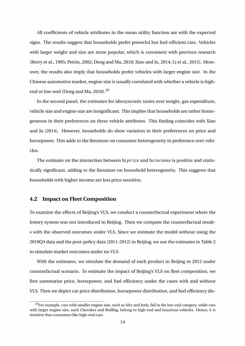
Table 3 compares the price, horsepower, and fuel efficiency of the cohort of new pas-

senger vehicles registered in Beijing in 2012 with and without VLS. From Table 3, there are

significant differences in price, horsepower, and fuel efficiency. Our results indicate that,

under the VLS, the sales-weighted average price in Beijing in 2012 increased in about 62,440

Yuan; a 34.48% increase. We also find that the sales-weighted average horsepower under

the lottery was about 12.25% higher than that under counterfactual scenario of no policy.

Moreover, the fleet becomes less fuel-efficient. The sales-weighted average fuel efficiency of

new vehicles registered under the lottery was 12.85 km/liter, relative to 13.41 km/liter under

no policy. These results are consistent with our discussion above: the lottery system shifts

the new fleet in Beijing toward high-end and more powerful but less fuel-efficient vehicles.

Table 3: Price, Horsepower, and Fuel Efficiency Summary Statistics in Beijing in 2012

Without VLS With VLSVariables Mean S.D. Mean S.D. Difference

Price (1,000 Yuan) 181.11 171.74 243.55 213.67 62.44∗∗∗

Horsepower (kw) 100.98 31.30 113.35 37.28 12.37∗∗∗

Fuel Efficiency(km/L) 13.41 2.09 12.85 2.29 -0.56∗∗∗

Note: All money is in 2012 RMB Yuan. The mean of price, horsepower, andfuel efficiency are sales-weighted means. The new vehicle sales are 949,950under counterfactual scenario and 527,183 under observed scenario in 2012.*** significant at 1%; ** significant at 5%; * significant at 10%.

With the derived demand for each product and the total sales, we calculate the cumu-

lative density function (CDF) of car prices, horsepower, and fuel efficiency, and plot their

distributions. We depict the price distribution, horsepower distribution, and fuel efficiency

distribution in Figure 4, 5, and 6, respectively. As shown in Figure 4, the cumulative distribu-

tion of prices under the lottery system lies to the right of that under counterfactual scenario

of no VLS. This implies that households would buy more expensive cars under the lottery

system. Similarly, Figure 5 and 6 indicate that the cumulative distribution of horsepower

shifts to the left and fuel efficiency lie to the right, relative to the counterfactual scenario of

no policy. That is, the lottery system increases the sales proportion of more powerful but

15

less fuel-efficient cars.

Figure 4: The CDF of Price of New Cars Registered in Beijing in 2012

Figure 5: The CDF of Horsepower of New Cars Registered in Beijing in 2012

4.3 Why Does Fleet Composition Change after VLS

Our analysis finds that the fleet of new passenger cars shifts towards high-end, less fuel-

efficient vehicles. Yang et al. (2014) also note this tendency because households would

16

Figure 6: The CDF of Fuel Efficiency of New Cars Registered in Beijing in 2012

spend all the transportation investments on more expensive vehicles due to VLS. However,

conditional on entering the lottery, the lottery system randomly assigns licenses to buyers

in the lottery pool. Therefore, winning the lottery is not correlated with the characteristics

of the households. So the winners’ purchase preferences and vehicle choices may not be

affected. The purpose of this section is to offer a possible explanation for the result of our

analysis from the perspective of how VLS affects households’ entering lottery decisions.

Under VLS, a household’s decisions can be divided into two stages, as shown in Figure

7. In the stage 1, the household decides whether to enter the lottery. The household on-

ly obtain utility Unot aenter from consumption of other commodities (i.e., complex good) if

he does not enter the lottery. If the household decides to enter the lottery, then we move

to stage 2. Upon entering, the household wins the lottery with probability of δ. Once the

household wins the lottery, he chooses the most preferred vehicle j , obtaining utility U j

from consuming car and from consumption of a numeraire good. Otherwise, the household

only consumes complex good with utility of U0. We employ backward induction to illustrate

the problem.

Stage 2. The household’s indirect utility from choosing vehicle j is U j = U (y − p j ,q j ),

where y is the household income, p j and q j are vehicle j ’s price and non-price character-

istics, respectively. Following Herriges and Kling (1999), we assume additive utilities, i.e.,

17

Figure 7: Two Stages of a Household’s Decisions under VLS

U j =V (y −p j )+ f (q j ). Here, f (q j ) is the utility from consuming vehicle j . And V (·) denotes

the utility from consumption of numeraire good. So the utility function satisfies standard as-

sumptions in the literature: (1) twice continuously differentiable, (2) strictly increasing, i.e.,

V ′(·) > 0, (3) strictly concave, i.e., V ′′(·) < 0, and (4) Inada conditions, i.e., limx→0 V ′(x) =∞and limx→∞V ′(x) = 0. If the household loses the lottery, the utility is U0 = V (y). As a result,

the expected utility in stage 2 is:

EU = δU j + (1−δ)U0 = δV (y −p j )+δ f (q j )+ (1−δ)V (y)

Stage 1. In this stage, the household decides whether to enter the lottery. If the house-

hold does not enter, the indirect utility is defined by Unot aenter =V (y)+ε0. As noted in stage

2, the indirect utility of entering the lottery is specified as Uenter = δV (y − p j )+δ f (q j )+(1−δ)V (y)+ε1. Here, ε0 and ε1 follows i.i.d. type I extreme value distribution. Hence, the

conditional probability of entering the lottery can be written as

Prob(enter) =exp[δV (y −p j )+δ f (q j )+ (1−δ)V (y)]

exp[V (y)]+exp[δV (y −p j )+δ f (q j )+ (1−δ)V (y)]

Taking derivative with respect to y and rearranging the equation, we obtain

∂Prob(enter)

∂y= Prob(enter) · [1−Prob(enter)] ·δ · [V ′(y −p j )−V ′(y)]

18

Given V ′(·) > 0, V ′′(·) < 0, and y − p j < y , it implies V ′(y − p j )−V ′(y) > 0. Therefore,

we find ∂Prob(enter)∂y > 0, meaning that high income households are more likely to enter the

lottery. Although the VLS randomly assigns licenses to buyers in the lottery pool, wealthi-

er consumers enter the lottery due to the policy. Proportion of winners with high income

increases. High income household would buy more expensive vehicles and therefore the

fleet shifts toward high-end but less fuel-efficient cars. Li et al. (2015) also provide addi-

tional evidence to support our illustration. In their stated preference survey conducted in

Guangzhou, the average income of lottery participants ranks second, which comes after that

of bidding participants.

5 Conclusion

With the rapid growth in vehicle population, problems such as congestion, energy short-

ages, air pollution and its health consequences have become a major concern in Beijing and

other cities worldwide. To control vehicle growth and thereby address related environmen-

tal issues, Beijing’s municipal government imposed a vehicle quota system and allocated

the quota through lottery. In this paper, we investigate the impacts of such novel policy on

fleet composition. To do this, we estimate a random coefficient discrete choice model of

automotive oligopoly using registration data of new passenger vehicles in Beijing, Nanjing,

Shenzhen, and Tianjin. To identify the effects of the lottery, we then conduct counterfactual

analysis based on the model estimates.

Our main result suggests vehicle fleet composition changes due to the VLS, shifting it

towards less fuel-efficient cars. This change can undermine the potential benefits of the

VLS. We further illustrate the underlying mechanism of this finding with a theoretical model.

It suggests that households with higher income are more likely to enter the lottery. As a

result, the proportion of wealthy households in the pool increases. This drives the demand

towards high-end vehicles, since high income household would purchase these cars. Our

result would provide the policy market a guideline of what to expect if a similar policy is

implemented in other cities.

19

The VLS in Beijing has been emulated in Guiyang, Guangzhou, Tianjin, Hangzhou, and

Shenzhen, and similar programs are being considered for other Chinese cities, such as Cheng-

du and Wuhan. Our analysis suggests that VLS hinders fleet fuel efficiency due to its impact

on fleet composition. As a result, VLS could still be improved by setting detailed quotas for

fuel efficiency categories or engine size categories.

20

References

Bento, Antonio M., Lawrence H. Goulder, Mark R. Jacobsen, and Roger H. von Haefen. 2009.

“Distributional and Efficiency Impacts of Increased US Gasoline Taxes.” American Eco-

nomic Review, 99(3): 667–699.

Berry, Steven, James Levinsohn, and Ariel Pakes. 1995. “Automobile Prices in Market Equi-

librium.” Econometrica, 63(4): 841–890.

Berry, Steven, James Levinsohn, and Ariel Pakes. 2004. “Differentiated Products Demand

Systems from a Combination of Micro and Macro Data: The New Car Market.” Journal of

Political Economy, 112(1): 68–105.

Davis, Lucas W. 2008. “The Effect of Driving Restrictions on Air Quality in Mexico City.” Jour-

nal of Political Economy, 116(1): 38–81.

Deng, Haiyan, and Alyson C. Ma. 2010. “Market Structure and Pricing Strategy of China’s

Automobile Industry.” Journal of Industrial Economics, 58(4): 818–845.

Dubé, Jean-Pierre, Jeremy T. Fox, and Che-Lin Su. 2012. “Improving the Numerical Perfor-

mance of Static and Dynamic Aggregate Discrete Choice Random Coefficients Demand

Estimation.” Econometrica, 80(5): 2231–2267.

Eliasson, Jonas, Lars Hultkrantz, Lena Nerhagen, and Lena Smidfelt Rosqvist. 2009. “The

Stockholm congestion – charging trial 2006: Overview of effects.” Transportation Research

Part A: Policy and Practice, 43(3): 240–250.

Fullerton, Don, and Li Gan. 2005. “Cost-Effective Policies to Reduce Vehicle Emissions.”

American Economic Review, 95(2): 300–304.

Gallego, Francisco, Juan-Pablo Montero, and Christian Salas. 2013. “The effect of transport

policies on car use: Evidence from Latin American cities.” Journal of Public Economics,

107 47–62.

Gibson, Matthew, and Maria Carnovale. 2015. “The effects of road pricing on driver behavior

and air pollution.” Journal of Urban Economics, 89 62–73.

21

Goldberg, Pinelopi Koujianou. 1998. “The Effects of the Corporate Average Fuel Efficiency

Standards in the US.” Journal of Industrial Economics, 46(1): 1–33.

Hao, Han, Hewu Wang, and Minggao Ouyang. 2011. “Comparison of Policies on Vehicle

Ownership and Use between Beijing and Shanghai and Their Impacts on Fuel Consump-

tion by Passenger Vehicles.” Energy Policy, 39(2): 1016–1021.

Herriges, Joseph A., and Catherine L. Kling. 1999. “Nonlinear Income Effects in Random U-

tility Models.” Review of Economics and Statistics, 81(1): 62–72.

Li, Jun, Pinjie Wu, and Wenna Zhang. 2015. “Car Ownership Choice Analysis under the Vehi-

cle Quota Restriction Policy: A Case Study of Guangzhou.” International Journal of Emer-

gin Engineering Research and Technology, 3(2): 92–102.

Li, Peiheng, and Steven Jones. 2015. “Vehicle restrictions and CO2 emissions in Beijing – A

simple projection using available data.” Transportation Research Part D: Transport and

Environment, 41 467–476.

Li, Shanjun. 2017. “Better Lucky Than Rich? Welfare Analysis of Automobile License Alloca-

tions in Beijing and Shanghai.” Review of Economic Studies, forthcoming.

Li, Shanjun, Junji Xiao, and Yimin Liu. 2015. “The Price Evolution in China’s Automobile

Market.” Journal of Economics and Management Strategy, 24(4): 786–810.

Parry, Ian W. H., and Kenneth A. Small. 2005. “Does Britain or the United States Have the

Right Gasoline Tax?” American Economic Review, 95(4): 1276–1289.

Petrin, Amil. 2002. “Quantifying the Benefits of New Products: The Case of the Minivan.”

Journal of Political Economy, 110(4): 705–729.

Seik, Foo Tuan. 1998. “A Unique Demand Management Instrument in Urban Transport: The

Vehicle Quota System in Singapore.” Cities, 15(1): 27–39.

Small, Kenneth A., Clifford Winston, and Jia Yan. 2005. “Uncovering the Distribution of Mo-

torists’ Preferences for Travel Time and Reliability.” Econometrica, 73(4): 1367–1382.

22

Train, Kenneth E. 2009. Discrete choice methods with simulation.: Cambridge University

Press.

Viard, V. Brian, and Shihe Fu. 2015. “The effect of Beijing’s driving restrictions on pollution

and economic activity.” Journal of Public Economics, 125 98–115.

Wolff, Hendrik. 2014. “Keep Your Clunker in the Suburb: Low-Emission Zones and Adoption

of Green Vehicles.” Economic Journal, 124(578): 481–512.

Wolff, Hendrik, and Lisa Perry. 2010. “Policy Monitor: Trends in Clean Air Legislation in Eu-

rope: Particulate Matter and Low Emission Zones.” Review of Environmental Economics

and Policy, 4(2): 293–308.

Xiao, Junji, and Heng Ju. 2014. “Market Equilibrium and the Environmental Effects of Tax

Adjustments in China’s Automobile Industry.” Review of Economics and Statistics, 96(2):

306–317.

Xiao, Junji, and Xiaolan Zhou. 2013. “An Empirical Assessment of the Impact of the Vehicle

Quota System on Environment: Evidence from China.” School of Management, Fudan

University.

Xiao, Junji, Xiaolan Zhou, and Wei-Min Hu. 2017. “Welfare Analysis of the Vehicle Quota

System in China.” International Economic Review, 58(2): 617–650.

Yang, Jun, Antung A. Liu, Ping Qin, and Joshua Linn. 2016. “The Effect of Owning a Car on

Travel Behavior: Evidence from the Beijing License Plate Lottery.” Working Paper.

Yang, Jun, Ying Liu, Ping Qin, and Antung A. Liu. 2014. “A review of Beijing’s vehicle registra-

tion lottery: Short-term effects on vehicle growth and fuel consumption.” Energy Policy,

75 157–166.

23