a least absolute deviation tuning method to reduce signal

26

BIU Journal of Basic and Applied Sciences 1(1): 26 – 39, 2015.

©Faculty of Basic and Applied Sciences, Benson Idahosa University, Benin City, Nigeria

A LEAST ABSOLUTE DEVIATION TUNING METHOD TO REDUCE SIGNAL

COVERAGE LOSS PREDICTION ERROR IN ELECTROMAGNETIC WAVE

PROPAGATION CHANNEL

*ISABONA, J.1

AND ENAGBONMA, O.2

1Department of Basic Sciences (Physics Unit), Benson Idahosa University, PMB.1100,

Benin City, Nigeria 2Department of Mathematics and Computer Sciences, Benson Idahosa University,

PMB.1100, Benin City, Nigeria.

*Corresponding author: [email protected]

ABSTRACT

The demand for increased mobile phone subscribers require an efficient radio network

planning that involves an accurate prediction of propagation loss. Although various

empirical loss models are in use, they are suitable for a particular environment or a

specific cell radius. The tuning of a model is a process in which the parameters of the

theoretical propagation model are adjusted with the help of measured values obtained

from the experimental data. In this process, several model parameters can be changed.

The objective of tuning is to obtain the values of the predicted model parameters to have

a closest match with minimal prediction error to the experimentally measured data. In

this paper, we have introduced a tuned least absolute deviation (LAD)-based

Walficsh/Ikegami (W/I) model using measured UMTS strength data carried out in GRA,

Benin City, Nigeria. We found that the performance of the tuned W/I model is the best as

root mean square error is lower compared to least square based regression technique.

The tuned model with LAD method best fit into BS 2 and BS 3 with an RMSE of 5.41 as

compared to least square tuning method which has an average RMSE of 16.68 with BS 2

and BS 3. This successfully validates our tuning methodology and suggests that the tuned

model is more accurate for the specified environment.

KEYWORDS: Optimization, Propagation Model Tuning, least absolute deviation

regression method, prediction error, electromagnetic waves,

environment.

INTRODUCTION

In wireless communication

technologies, information is sent by

electromagnetic waves. Electromagnetic

wave propagation in real space is very

complicated and much more complex in

the mobile communication system, which

are mainly displayed in three aspects

(Tiegang, (2013):

(i) The openness of wireless channel-

When electromagnetic wave

transmits in open space, the wireless

27

channels are easily affected by all

kinds of interference signals.

(ii) The complexity and diversity of

propagation environment- The

mobile communication system works

both in big cities with high buildings

and small villages in mountains.

(iii) The random mobility of users-Users

might call anywhere, such as in

rooms, in a high-speed train or car.

Above three aspects have a great

influence on the propagation of

electromagnetic wave in a mobile

communication system; during

propagation an interaction between waves

and environment attenuates the signal

level. It causes path loss and finally it

limits coverage area. Generally, wireless

propagation models are built to predict

the path loss, so as to estimate the field

strength coverage of received signals.

The accurate signal coverage prediction

using propagation pathloss models is a

crucial element in the first step of

network planning. The capability of

determining optimum Base-Station (BS)

locations, obtaining suitable data rates

and estimating coverage without

conducting a series of propagation

measurements (what is very expensive

and time consuming) can be achieved

with propagation models.

Propagation models commonly used

in mobile communication network

planning are mostly empirical models,

which are mathematical model

summarized from a large number of

measured data, for example, Okumura-

Hata’s model, COST231-Hata model,

COST231-Walfisch-Ikegami model and

SPM model, etc.

Empirical propagation models are

designed for a specific type of

communication systems, specific system

parameters and types of environment.

This is due to the different propagation

characteristics which are in different

areas. Thus, if empirical models are

mechanically copied in all areas, a great

error will generate between calculation

results and actual values.

Especially in Nigeria, because of the

vast area of the country and various types

of geography in different places, if you

want to apply a model in different

regions, some parameters must be

modified, which means that a model

correction is needed. This is to reduce its

propagation prediction errors. There are

mainly two sources causing the errors

(Tiegang, 2013): errors from test data for

correction and error from correction

algorithm. Errors from test data are

mainly composed of three aspects: GPS

errors, digital map errors, and CW

(Continuous Wave) test equipment errors.

GPS errors depend on the measuring

accuracy of GPS equipment; digital map

Errors depend on the resolution of digital

maps; CW test equipment errors, on one

hand, result from the test device itself, on

the other hand, from improper operation.

In this paper, the Least Absolute

Deviation (LD) method is introduced to

effectively reduce the errors via

propagation model tuning procedure. We

will describe the method through the

example of COST-231 Walficsh-Ikegami

(W/I) model correction.

MATERIALS AND METHODS

With the rapid growth of the

telecommunication industry in Nigeria,

all operators are paying more and more

Isabona, J. & Enagbonma, O. A Least Absolute Deviation Tuning Method to Reduce Signal Coverage

28

attention to the matching extent between

propagation model and local

environment. In this environment, high

quality of service is a competitive

advantage for a service provider. The

radio propagation environment is very

complicated, and the otherness between

different areas is great, so it is necessary

to carry actual propagation model testing

and tuning, and then obtain the

propagation model which reflects radio

propagation characteristic exactly

(Wenxiao and Mingjing, 2008).

In recent times, operators usually use

special planning software to finish

propagation model tuning. Now, there are

several kinds of popular radio network

planning software, such as ASSET

software of AIRCOM Company in

England, PLANET software of

MARCONI Company in England and

ATOLL software of FOSK Company in

France (Lui et al., 2007)). Though using

planning software to model tuning is

convenient, this software depend on

digital map badly, the cost is expensive,

especially in some small and medium-

sized cities (Wenxiao and Mingjing,

2008). Thus, the process of tuning

propagation models is very important,

and can have major impact on their

accuracy.

A statistical tuning method based on

least-square theory for adjusting the

Walfisch-Bertoni model parameters for

generalized conditions in the CDMA2000

signal propagation environments was

previously proposed (Isabona and Azi,

2012). However, this method relates to

many tuning parameters, the iterative

tuning process is relatively complicated.

In this paper, we engage simple linear-

iterative Least Absolute (LAD) method

for automatics model tuning and

obtaining an exact outdoor propagation

model fitting for UMTS signal

propagation data in the studied

environment. This method, as the name

suggests, minimizes not the sum of

squared deviations but the sum of

absolute values of the deviations.

Consequently it does not put excessive

weight on highly deviating observations

like the least squares does, and hence

produces more robust estimators with

respect to outliers. This is important to

direct a more robust planning of present

and future cellular wireless

communication systems in Nigeria.

Theory of Propagation Model Tuning

The quality of a network plan is

dependent on the accuracy of the

propagation model used to produce

coverage plots and conduct interference

analysis. An unreliable propagation

model will result in a poor network plan,

with too many sites (i.e. investing too

much) or too few sites (i.e. not meeting

the service requirements and a huge cost

to rectify the situation). Propagation

model tuning includes defining the clutter

classes, CW measurements of those

different clutter classes, statistical

analysis of the measurements, tuning of

the planning propagation models and

parameters and final selection of

propagation models, clutter classes and

tuned parameters. Tuning the propagation

model is an iterative process which

requires defining new clutter classes to

obtain better results.

The objective of propagation model

tuning is to obtain values for model

parameters that are in agreement with

measured data. When using these tuned

parameters, the median of the predicted

BIU Journal of Basic and Applied Sciences Vol. 1 no. 1 (2015)

29

path loss shall have a minimum

difference and variance when compared

to median of measured path loss. The

tuning or calibration process can be

achieved either manually or

automatically. The manual tuning process

consists of adjustment of the model

parameters in order to set the error

between measured and predicted signals

near or equal to zero. We then increment

the parameters one by one. These

processes are repeated manually until any

change in parameters will increase error

value. The manual tuning process

requires a large number of repetitions

before a near global minimum is

obtained.

CW Measurement and Measured

Propagation loss Data Totaling

The CW measurements were

conducted from a UMTS network base

station (BS) transmitters, located at the

BIU Campus, Ugbor and Gapiona

Avenues, all evenly distributed in

Government Reserved Area (GRA),

Benin City, Edo Sate, Nigeria. Each of

the BSs in the three study locations are

tagged BS 1, BS 2 and BS 3 in this paper.

The measured CW received signal

strength data which is the Received

Signal Code Power (RSCP) and

transmitter-receiver (T-R) separation

distance (d) are recorded in dBm and m.

Every measurement points of received

signal strength and T-R separation

distance are recorded evenly from all the

predefined routes of three base stations.

Each measurement point is represented in

an average of a set of samples taken over

a small area (10m2) in order to remove

the effects of fast fading (Takahashi,

2004). A CW drive-test system was used

to collect and record signal level data at

various locations in a form of logs which

were later processed with a

communication network analyzer. The

CW drive test process used here is broken

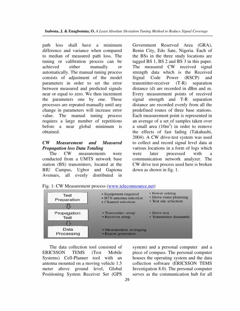
down as shown in fig. 1.

Fig. 1: CW Measurement process (www.telecomsource.net)

The data collection tool consisted of

ERICSSON TEMS (Test Mobile

Systems) Cell-Planner tool with an

antenna mounted on a moving vehicle 1.5

meter above ground level, Global

Positioning System Receiver Set (GPS

system) and a personal computer and a

piece of compass. The personal computer

houses the operating system and the data

collection software (ERICSSON TEMS

Investigation 8.0). The personal computer

serves as the communication hub for all


30

other equipment in the system. The GPS

operates with global positioning satellites

to provide the location tracking for the

system during data collection position on

a global map which has been installed on

the personal computer. The compass help

to determine the various azimuth angles

of the base station transmitters. Average

height of transmit antenna is about 30–32

meters above ground level, with the same

transmit power. Sampling rate of the

collected data, on the average, is about 2–

3 samples per meter. The transmission

parameters are given in table 1.

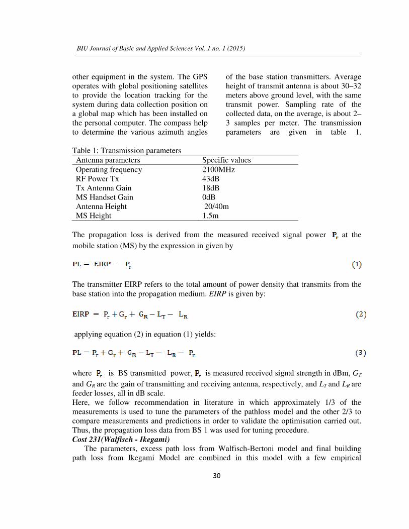
Table 1: Transmission parameters

Antenna parameters Specific values

Operating frequency 2100MHz

RF Power Tx 43dB

Tx Antenna Gain 18dB

MS Handset Gain 0dB

Antenna Height 20/40m

MS Height 1.5m

The propagation loss is derived from the measured received signal power at the

mobile station (MS) by the expression in given by

The transmitter EIRP refers to the total amount of power density that transmits from the

base station into the propagation medium. EIRP is given by:

applying equation (2) in equation (1) yields:

where is BS transmitted power, is measured received signal strength in dBm, GT

and GR are the gain of transmitting and receiving antenna, respectively, and LT and LR are

feeder losses, all in dB scale.

Here, we follow recommendation in literature in which approximately 1/3 of the

measurements is used to tune the parameters of the pathloss model and the other 2/3 to

compare measurements and predictions in order to validate the optimisation carried out.

Thus, the propagation loss data from BS 1 was used for tuning procedure.

Cost 231(Walfisch - Ikegami) The parameters, excess path loss from Walfisch-Bertoni model and final building

path loss from Ikegami Model are combined in this model with a few empirical


31

correction parameters. This model is statistical and not deterministic because you can

only insert a characteristic value, with no considerations of topographical database of

buildings. The model is restricted to flat urban terrain.

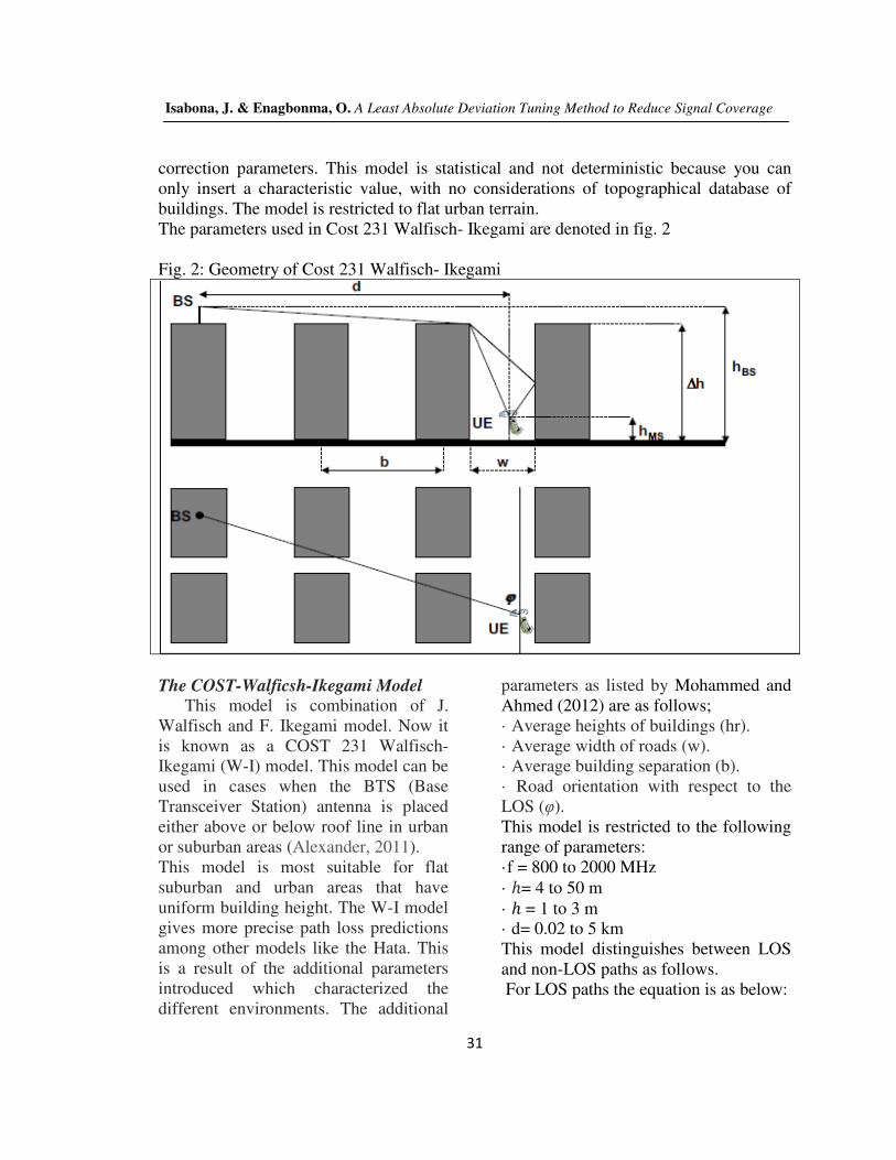
The parameters used in Cost 231 Walfisch- Ikegami are denoted in fig. 2

Fig. 2: Geometry of Cost 231 Walfisch- Ikegami

The COST-Walficsh-Ikegami Model This model is combination of J.

Walfisch and F. Ikegami model. Now it

is known as a COST 231 Walfisch-

Ikegami (W-I) model. This model can be

used in cases when the BTS (Base

Transceiver Station) antenna is placed

either above or below roof line in urban

or suburban areas (Alexander, 2011).

This model is most suitable for flat

suburban and urban areas that have

uniform building height. The W-I model

gives more precise path loss predictions

among other models like the Hata. This

is a result of the additional parameters

introduced which characterized the

different environments. The additional

parameters as listed by Mohammed and

Ahmed (2012) are as follows;

· Average heights of buildings (hr).

· Average width of roads (w).

· Average building separation (b).

· Road orientation with respect to the

LOS (φ).

This model is restricted to the following

range of parameters:

·f = 800 to 2000 MHz

· ℎ= 4 to 50 m

· ℎ = 1 to 3 m

· d= 0.02 to 5 km

This model distinguishes between LOS

and non-LOS paths as follows.

For LOS paths the equation is as below:


32

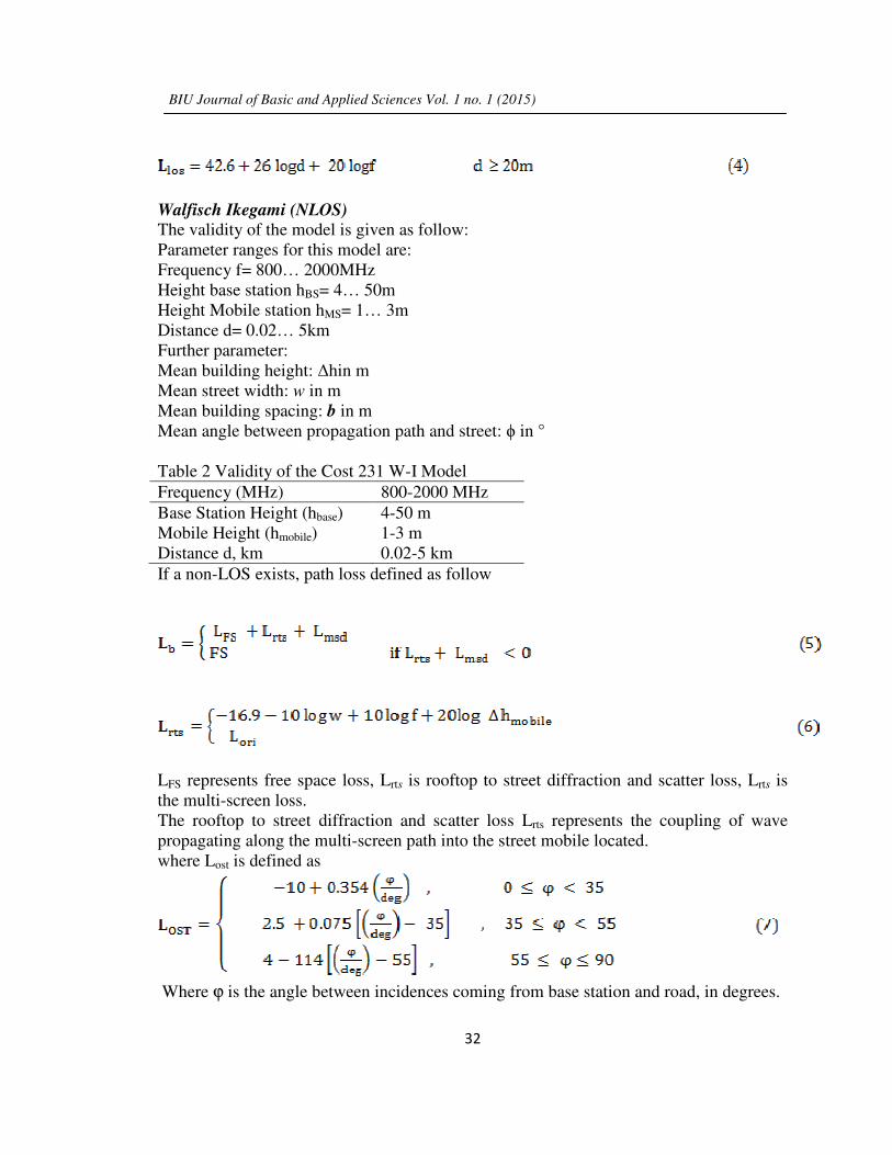
Walfisch Ikegami (NLOS) The validity of the model is given as follow:

Parameter ranges for this model are:

Frequency f= 800… 2000MHz

Height base station hBS= 4… 50m

Height Mobile station hMS= 1… 3m

Distance d= 0.02… 5km

Further parameter:

Mean building height: Δhin m

Mean street width: w in m

Mean building spacing: b in m

Mean angle between propagation path and street: ϕ in °

Table 2 Validity of the Cost 231 W-I Model

Frequency (MHz) 800-2000 MHz

Base Station Height (hbase) 4-50 m

Mobile Height (hmobile) 1-3 m

Distance d, km 0.02-5 km

If a non-LOS exists, path loss defined as follow

LFS represents free space loss, Lrts is rooftop to street diffraction and scatter loss, Lrts is

the multi-screen loss.

The rooftop to street diffraction and scatter loss Lrts represents the coupling of wave

propagating along the multi-screen path into the street mobile located.

where Lost is defined as

Where ϕ is the angle between incidences coming from base station and road, in degrees.


33

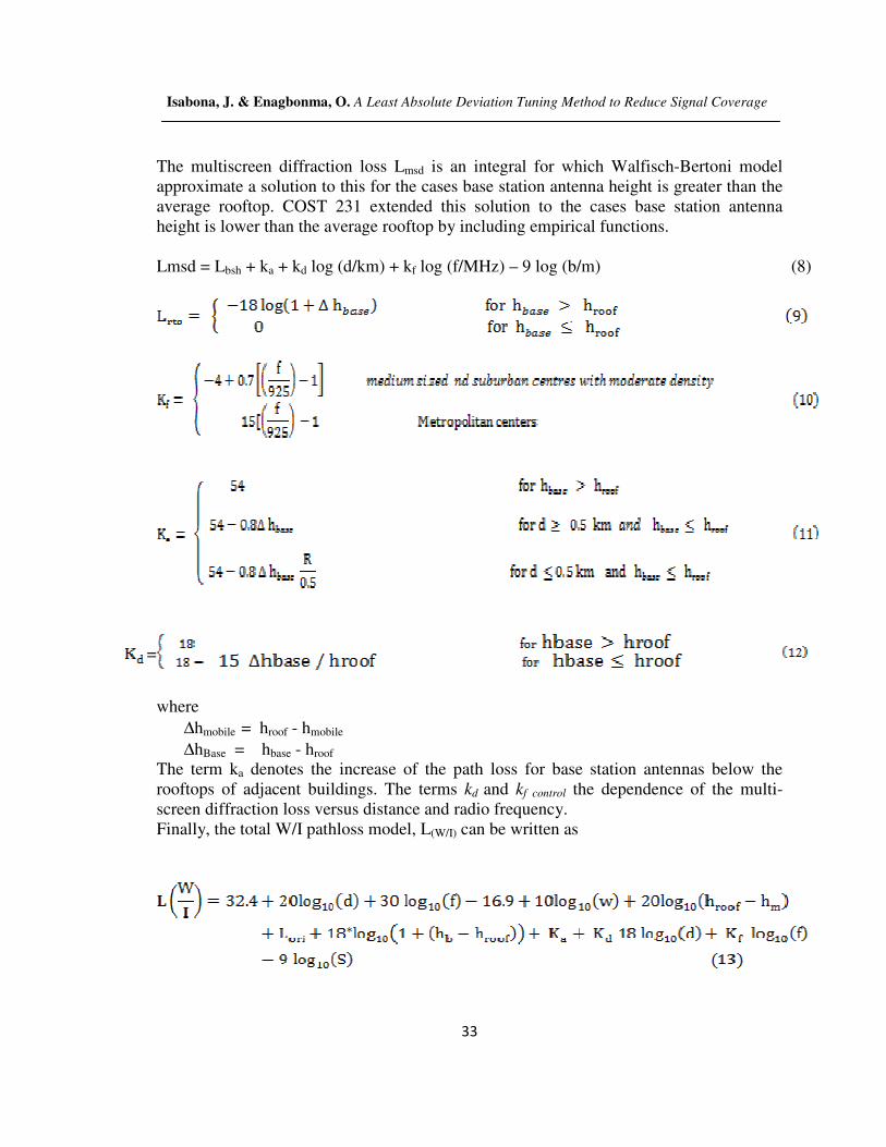
The multiscreen diffraction loss Lmsd is an integral for which Walfisch-Bertoni model

approximate a solution to this for the cases base station antenna height is greater than the

average rooftop. COST 231 extended this solution to the cases base station antenna

height is lower than the average rooftop by including empirical functions.

Lmsd = Lbsh + ka + kd log (d/km) + kf log (f/MHz) – 9 log (b/m) (8)

where

∆hmobile = hroof - hmobile

∆hBase = hbase - hroof

The term ka denotes the increase of the path loss for base station antennas below the

rooftops of adjacent buildings. The terms kd and kf control the dependence of the multi-

screen diffraction loss versus distance and radio frequency.

Finally, the total W/I pathloss model, L(W/I) can be written as

=


34

It is impossible to represent with

total reliability all the features of an

environment; consequently, the

propagation models use approximations

and suppositions (they consider

buildings as half edges, they

approximate to zero the absorption of the

walls, etc), those suppositions cause

error in simulation results. Although

Walfisch Ikegami model of equation

(11) was designed for BS antennas

placed below the mean building height,

however, the model show often

considerable inaccuracies. This is

especially true in cities with an irregular

building pattern like in historical grown

cities. Also the model was designed for

cities on a flat ground. Thus for cities in

a hilly environment the model is not

applicable

Model Tuning Process

Overview This work proposes a method that

consists of statistical model correction

through the multiple linear regression of

the absolute difference from the

propagation loss data obtained by the

W/I (11) in relation to the environment

and the propagation loss data collected

in the studied environment

The W/I propagation model equation is

multivariate, one variable, L. In order to

correct the W/I model to field data, we

will multiply the model’s default

parameters in Eq.1 with variables and

this gives:

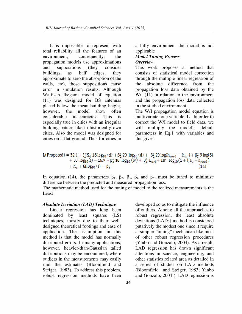
In equation (14), the parameters β1, β2, β3, β4 and β5, must be tuned to minimize

difference between the predicted and measured propagation loss.

The mathematic method used for the tuning of model to the realized measurements is the

Least

Absolute Deviation (LAD) Technique

Linear regression has long been

dominated by least squares (LS)

techniques, mostly due to their well-

designed theoretical footings and ease of

application. The assumption in this

method is that the model has normally

distributed errors. In many applications,

however, heavier-than-Gaussian tailed

distributions may be encountered, where

outliers in the measurements may easily

ruin the estimates (Bloomfield and

Steiger, 1983). To address this problem,

robust regression methods have been

developed so as to mitigate the influence

of outliers. Among all the approaches to

robust regression, the least absolute

deviations (LADs) method is considered

putatively the modest one since it require

a simpler “tuning” mechanism like most

of other robust regression procedures

(Yinbo and Gonzalo, 2004). As a result,

LAD regression has drawn significant

attentions in science, engineering, and

other statistics related area as detailed in

a series of studies on LAD methods

(Bloomfield and Steiger, 1983; Yinbo

and Gonzalo, 2004 ). LAD regression is


35

based on the assumption that the model

has Laplacian distributed errors (Yinbo

and Gonzalo, 2004).

Given the pathloss data set, ynwith n

measurements, which depend on the

input variables x1, x2… xp, x∈Ν, then we

consider a LAD regression model

This model is to be fitted of n, n ∈ Ν points

yi, xi1, xi2,…,xip, i = 1, 2,…., n.

The observations yi, where i = 1, 2…, n will be represented by a vector Y. The unknowns

β1, β2… βp will be represented by a vector Y. Let X be a matrix.

For a given β, the vector of fitted or predicted values, Lp, can be written Lp = X β. Using

the LAD estimation we will pick the coefficients β = (β1, β2… βp)T to minimize the

residual sum of absolute values (RSA), i.e,

Differentiating RSA with respect to β, we get

For all real vectors β for which the function is differentiable, sign is the sign of the

variables.

Thus, RSS is minimal for

Here, the differential correction in equation (17) is implemented using JavaScript

program. It involves expanding the function to be fitted in a Taylor series around current

estimates of the parameters, retaining first-order (linear) terms, and solving the resulting

linear system for incremental changes to the parameters. The program computes finite-

difference approximations to the required partial derivatives, and then uses a simple

elimination algorithm to invert and solve the equations.

RESULTS

The tuned Walficsh-Ikegami (W/I)

model parameters with measured

propagation loss data using LAD

regression method are given in table 3.

Shown in table 4 are the tuned parameters

of W/I model using LS regression

technique; this was done for comparison

and to verify the correctness of our

proposed tuning approach utilized in this

paper.


36

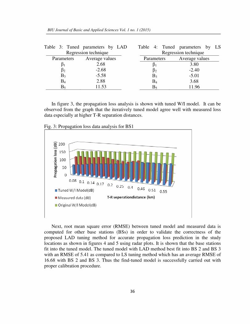
Table 3: Tuned parameters by LAD

Regression technique

Parameters Average values

β1 2.68

β2 -2.68

Β3 -5.58

Β4 2.88

Β5 11.53

Table 4: Tuned parameters by LS

Regression technique

Parameters Average values

β1 3.80

β2 -2.40

Β3 -5.01

Β4 3.68

Β5 11.96

In figure 3, the propagation loss analysis is shown with tuned W/I model. It can be

observed from the graph that the iteratively tuned model agree well with measured loss

data especially at higher T-R separation distances.

Fig. 3: Propagation loss data analysis for BS1

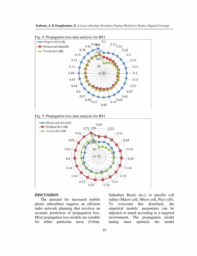
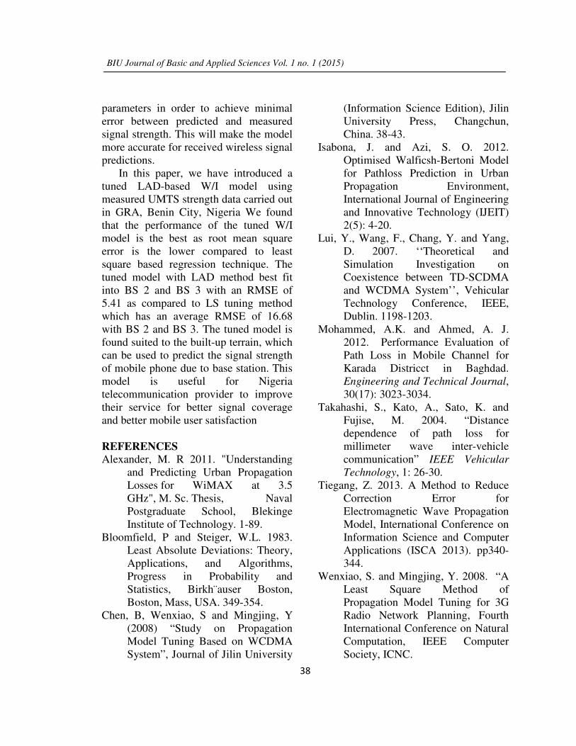
Next, root mean square error (RMSE) between tuned model and measured data is

computed for other base stations (BSs) in order to validate the correctness of the

proposed LAD tuning method for accurate propagation loss prediction in the study

locations as shown in figures 4 and 5 using radar plots. It is shown that the base stations

fit into the tuned model. The tuned model with LAD method best fit into BS 2 and BS 3

with an RMSE of 5.41 as compared to LS tuning method which has an average RMSE of

16.68 with BS 2 and BS 3. Thus the find-tuned model is successfully carried out with

proper calibration procedure.


37



DISCUSSION

The demand for increased mobile

phone subscribers requires an efficient

radio network planning that involves an

accurate prediction of propagation loss.

Most propagation loss models are suitable

for either particular areas (Urban,

Suburban, Rural, etc.), or specific cell

radius (Macro cell, Micro cell, Pico cell).

To overcome this drawback, the

empirical models’ parameters can be

adjusted or tuned according to a targeted

environment. The propagation model

tuning must optimize the model


38

parameters in order to achieve minimal

error between predicted and measured

signal strength. This will make the model

more accurate for received wireless signal

predictions.

In this paper, we have introduced a

tuned LAD-based W/I model using

measured UMTS strength data carried out

in GRA, Benin City, Nigeria We found

that the performance of the tuned W/I

model is the best as root mean square

error is the lower compared to least

square based regression technique. The

tuned model with LAD method best fit

into BS 2 and BS 3 with an RMSE of

5.41 as compared to LS tuning method

which has an average RMSE of 16.68

with BS 2 and BS 3. The tuned model is

found suited to the built-up terrain, which

can be used to predict the signal strength

of mobile phone due to base station. This

model is useful for Nigeria

telecommunication provider to improve

their service for better signal coverage

and better mobile user satisfaction

REFERENCES

Alexander, M. R 2011. "Understanding

and Predicting Urban Propagation

Losses for WiMAX at 3.5

GHz", M. Sc. Thesis, Naval

Postgraduate School, Blekinge

Institute of Technology. 1-89.

Bloomfield, P and Steiger, W.L. 1983.

Least Absolute Deviations: Theory,

Applications, and Algorithms,

Progress in Probability and

Statistics, Birkh¨auser Boston,

Boston, Mass, USA. 349-354.

Chen, B, Wenxiao, S and Mingjing, Y

(2008) “Study on Propagation

Model Tuning Based on WCDMA

System”, Journal of Jilin University

(Information Science Edition), Jilin

University Press, Changchun,

China. 38-43.

Isabona, J. and Azi, S. O. 2012.

Optimised Walficsh-Bertoni Model

for Pathloss Prediction in Urban

Propagation Environment,

International Journal of Engineering

and Innovative Technology (IJEIT)

2(5): 4-20.

Lui, Y., Wang, F., Chang, Y. and Yang,

D. 2007. ‘‘Theoretical and

Simulation Investigation on

Coexistence between TD-SCDMA

and WCDMA System’’, Vehicular

Technology Conference, IEEE,

Dublin. 1198-1203.

Mohammed, A.K. and Ahmed, A. J.

2012. Performance Evaluation of

Path Loss in Mobile Channel for

Karada Districct in Baghdad.

Engineering and Technical Journal,

30(17): 3023-3034.

Takahashi, S., Kato, A., Sato, K. and

Fujise, M. 2004. “Distance

dependence of path loss for

millimeter wave inter-vehicle

communication” IEEE Vehicular

Technology, 1: 26-30.

Tiegang, Z. 2013. A Method to Reduce

Correction Error for

Electromagnetic Wave Propagation

Model, International Conference on

Information Science and Computer

Applications (ISCA 2013). pp340-

344.

Wenxiao, S. and Mingjing, Y. 2008. “A

Least Square Method of

Propagation Model Tuning for 3G

Radio Network Planning, Fourth

International Conference on Natural

Computation, IEEE Computer

Society, ICNC.


39

Yinbo, L. and Gonzalo, R. A. 2004. A

Maximum Likelihood Approach to

Least Absolute Deviation

Regression, EURASIP Journal on

Applied Signal Processing, vol. 12,

pp 1762–1769.

www.telecomsource.net, RF Planning

Bible from Telenor- Telecomm

Source, (Accessed February, 14,

2014)


a least absolute deviation tuning method to reduce signal

Documents