A Knowledge-and-Physical-Capital Model of International ...people.brandeis.edu/~cbown/conferences/mcculloch/Bergstrand.pdf · A Knowledge-and-Physical-Capital Model of International

A Knowledge-and-Physical-Capital Model of International Trade Flows,Foreign Direct Investment, and Multinational Enterprises

by Jeffrey H. Bergstrand and Peter Egger

for presentation at the conference

Is Free Trade Still Optimal in the 21st Century?

A Conference Celebrating Professor Rachel McCullochDepartment of Economics and the International Business School

Brandeis UniversityJune 15, 2007

A Knowledge-and-Physical-Capital Model of International Trade Flows,Foreign Direct Investment, and Multinational Enterprises

Jeffrey H. Bergstrand a,b,* , Peter Egger c,d,e

aDepartment of Finance, Mendoza College of Business, and Kellogg Institute for International Studies,University of Notre Dame, Notre Dame, IN 46556 USA

bCESifo, Munich, GermanycDepartment of Economics, University of Munich, Munich, Germany

dIFO Institute, Munich, GermanyeCESifo, Munich, Germany

Abstract

This paper addresses two important issues at the nexus of the literatures on international trade, foreigndirect investment (FDI), foreign affiliate sales (FAS), and multinational enterprises (MNEs). First, the introductionof a third internationally-mobile factor (physical capital) to the standard 2x2x2 “knowledge-capital” model of MNEswith skilled and unskilled labor allows us to resolve fairly readily the puzzle in the modern MNE literature thatforeign affiliate sales among two identical economies completely displace their international trade. Intra-industrytrade and intra-industry FDI (and FAS) can coexist for national and multinational firms (with identicalproductivities) in identical countries. Second, the introduction also of a third country to the model suggests a formalN-country theoretical rationale for estimating gravity equations of bilateral FDI flows and FAS, in a mannerconsistent with estimating gravity equations for bilateral trade flows.

March 2007

JEL Classifications: F11, F12, F21, F23Keywords: Foreign Direct Investment, International Trade, Multinational Firms, Gravity Equation

*Corresponding author. Department of Finance, Mendoza College of Business, and Kellogg Institute forInternational Studies, University of Notre Dame, IN 46556, USA. Tel.: +1 574 631 6761; fax: +1 574 631 5255.

E-mail address: [email protected] (J.H. Bergstrand).

Acknowledgements

We deeply appreciate extensive and insightful comments on earlier drafts by Eric van Wincoop, BruceBlonigen, Ron Davies, Amy Glass, David Hummels, Kishore Gawande, Keith Maskus, Jim Markusen, HowardSchatz, Deborah Swenson, Chong Xiang, two anonymous referees, and participants at presentations at PurdueUniversity, Syracuse University, Texas A&M University, the European Economic Association meetings (2005), andthe Empirical Investigations in International Trade conference at UC-Santa Cruz (2004). Bergstrand acknowledgesresearch funding from the Mendoza College of Business and Kellogg Institute for International Studies at NotreDame and Egger acknowledges research funding from the Austrian Science Fund through grant P17713-G05.

1Martin and Rey (2004) have advanced a theory of the gravity equation for bilateral portfolio investmentflows. However, no studies have developed a theory for the gravity equation for bilateral FDI stocks/flows.Recently, a few studies have offered theoretical rationales for estimating bilateral FAS gravity equations, cf.,Ghazalian and Furtan (2005), Kleinert and Toubal (2005), and Lai and Zhu (2006); however, these studies assumeexogenously heterogeneous productivities to generate coexistence of multinational and national firms, in the spirit ofthe model in Helpman, Melitz, and Yeaple (2004), and only explain FAS. By contrast, we motivate the endogenouscoexistence of country pairs’ horizontal MNEs and national firms sharing identical productivities, even for identicaleconomies. Moreover, by incorporating capital flows, we provide simultaneously theoretical rationales for trade,FAS, and FDI gravity equations, distinguishing explicitly between FDI (a measure of MNE capital flow) and FAS (ameasure of MNE production). Consequently, our analysis is in the spirit of the “new trade theory” where, as noted inHelpman (2006, p. 592), within-industry heterogeneity results from product differentiation and monopolisticcompetition, and heterogenous productivities among firms are unnecessary to explain large volumes of intra-industrytrade. Since our theoretical model will be static, conventional to the trade and knowledge-capital MNE literatures(cf., Markusen, 2002), bilateral “flows” and “stocks” are conceptually identical. In empirical work, however, flowsand stocks will be distinguished. Traditionally, gravity equations have used bilateral FDI stock data, cf., Blonigen,Davies, Waddell, and Naughton (2004).

I. Introduction

“Multinationals displace trade . . . .” (Markusen, 1995, p. 180)

“The cross-country pattern of FDI is quite well approximated by the ‘gravity’ relationship.”(Barba Navaretti and Venables, 2004, p. 32)

This paper addresses two important issues at the nexus of the literatures on international trade, foreign

direct investment (FDI), foreign affiliate sales (FAS), and multinational enterprises (MNEs). First, the modern 2x2x2

general equilibrium theory of MNEs summarized in Markusen (2002) implies that – in two countries with identical

absolute and relative factor endowments (other things equal) – horizontal MNEs’ foreign affiliate sales displace

completely national firms (with identical productivities) and trade between the two countries. However, the European

Union and the United States, for instance, have both the largest intra-industry bilateral foreign direct investment

flows (and FAS) and intra-industry trade flows. This is a puzzle. Second, while multi-country theoretical foundations

for the trade gravity equation are now well established (cf., Anderson and van Wincoop, 2004, and Feenstra, 2004,

ch. 5, for overviews), there have been virtually no formal N-country (N>2) theoretical frameworks provided in

international economics for estimating gravity equations of aggregate bilateral FDI, despite numerous empirical

studies over the past decade using the gravity equation to explain such flows.1 Blonigen, Davies, Waddell, and

Naughton (2004) note that the “gravity model is arguably the most widely used empirical specification for FDI” (p.

8). Yet the typical rationale for applying the gravity equation to bilateral FDI is by analogy to the trade gravity

equation, cf., Mutti and Grubert (2004, p. 339) and Blonigen (2005, p. 21). This suggests a puzzle similar to one

posed 30 years ago for trade: The gravity equation explains bilateral FDI empirically quite well . . . but why?

We suggest a simple, integrated solution to both puzzles. First, the introduction of a third factor – physical

capital – to the modern two-factor “knowledge-capital” model with only skilled and unskilled labor, combined with

the assumption that headquarters (plant) setups require human (physical) capital, implies that national exporting

2

2We are not the first to try to address this puzzle. Blonigen (2001) and Head and Ries (2001) introduceintermediate goods to address the issue. However, the nature of trade in these models is “vertical,” nor horizontal;Baldwin and Ottaviano (2001) argue that the “intermediates augmented proximity-versus-scale model still has tradeand FDI as substitutes” (p. 432). As an alternative, Baldwin and Ottaviano argue that obstacles to trade generate anincentive for multiproduct firms to simultaneously engage in FDI and trade, in the spirit of the Brander-Krugman“reciprocal-dumping” model for goods trade. Our focus on a third factor and third country is an alternative to this.

3See Lipsey (2002) for more on the distinction between FAS and FDI. The modern 2x2x2 MNE modelexplains trade and FAS simultaneously, but not FDI. As Markusen (2002) notes, “the models in this book areaddressed more closely to affiliate output and sales than to investment stocks” (p. 8). Similarly, the heterogeneousproductivities models cited in footnote 1 cannot explain FDI as these models have only one factor, immobile labor.

enterprises (NEs) can coexist with horizontal MNEs (HMNEs) in pairs of countries with identical relative and

absolute factor endowments (and all firms sharing identical technologies). With skilled labor not being the only

factor used to set up both plants and firms, skilled labor is not completely displaced from plant setups to firm setups

as two countries’ GDPs converge in size. In the 2x2x2 model of Markusen and Venables (2002), there is only a

(highly unlikely) unique combination of trade costs, investment costs and ratio of plant-to-firm setup costs where

NEs and HMNEs can coexist. By contrast, with three factors, NEs and HMNEs with identical productivities can

coexist over a wide range of combinations of trade costs, investment costs, and plant-to-firm setup costs due to the

endogenous adjustment of the relative price of human-to-physical capital. Intra-industry trade and FDI can coexist

for two identical countries.2 Moreover, the existence of human and physical capital allows distinguishing MNEs’

foreign affiliate production from MNEs’ capital flows, two different “concepts of FDI.”3

Second, while introducing a third factor implies coexistence of NEs and HMNEs for identically-sized

economies, this extension cannot explain empirically the “complementarity” of bilateral trade and FDI flows to GDP

similarity. Typical empirical gravity equations of international trade and FDI tend to suggest that both trade and FDI

from country i to country j should be positively related to the size and similarity of their GDPs. However, the

introduction of a third country – rest-of-world (ROW) – to our “knowledge-and-physical-capital” model can explain

readily the complementarity of bilateral trade, FDI, and FAS to changes in a pair of countries’ economic size and

similarity as typical to gravity equations. In a two-country world, gross multilateral and bilateral trade (or FAS) are

identical; NEs and HMNEs must substitute for one another when the two countries are identically sized in the face of

trade and investment costs. However, introducing a third country along with capital mobility allows two countries’

trade, FDI, and FAS to covary positively with increases in these two countries’ GDP similarity because the

“substitution effect” associated with exogenous trade-to-investment costs is potentially offset by a “complementarity

effect” generated by endogenous relative prices of physical-to-human capital interacting with the three countries’

economic sizes. With three countries, both bilateral trade and FAS are maximized when a pair of countries’ GDPs

are identical, unlike a two-country world. Moreover, the presence of the third country can explain why FDI from one

country to another is not maximized when GDPs are identical – which is observed empirically!

3

4We will not provide a theoretical framework that is the perfect complement to the Anderson and vanWincoop (2003) theoretical foundation using a “conditional” general equilibrium (GE) model, which enabled themto derive a closed-form, analytic solution for the trade gravity equation with unit GDP elasticities. Instead, we usean “unconditional” GE approach, where the allocation of bilateral flows across countries is non-separable fromproduction and consumption allocations within countries, whereas a “conditional” GE approach assumes separabilityof bilateral flows from production and consumption allocations, cf., Anderson and van Wincoop (2004). Our modelis in the spirit of Markusen (2002). The benefit of our approach is illuminating the endogenous determination ofrepresentative firms’ outputs, countries’ numbers of NEs vs. MNEs, allocation of MNEs’ capital between countries,etc. The cost is we forego a closed-form solution for the gravity equation, relying instead on regressions of“theoretical” flows (from a numerical GE model) on GDPs, etc. to motivate theoretically estimation of log-lineargravity equations for trade flows, FAS, and FDI flows. Shim (2005) extends the Anderson and van Wincoopconditional GE model to include FAS to further explain the “border puzzle”; however, Shim assumes exogenouslythe (unlikely) unique equilibrium in Markusen and Venables (2000) that generates coexistence of NEs and MNEs.

The complexity of the nonlinear relationships between trade, foreign affiliate sales, FDI, GDP sizes and

similarities, trade costs, and investment costs precludes closed-form solutions, such as the trade gravity equations

derived in Helpman and Krugman (1985) or Anderson and van Wincoop (2003). As in Markusen (2002), we must

employ a numerical version of the general equilibrium (GE) model to motivate the gravity-like relationships among

these variables. However, the theoretical relationships between the bilateral flows – trade, foreign affiliate sales, and

FDI – and GDP sizes and similarities demonstrated graphically are similar, but not identical. Consequently, to avoid

“ocular-metrics” and in the presence of approximation errors associated with the nonlinear relationships, we employ

regressions of “theoretical” flows on pairs of countries’ GDPs, trade and investment costs, and ROW GDP to

motivate theoretically and quantitatively that bilateral trade, FAS, and FDI flows’ economic determinants should be

“well-approximated” by gravity equations – yet not precisely the same gravity relationships.4

The remainder of the paper is as follows. Section 2 presents some typical empirical regression results for

trade and FDI gravity equations to motivate our analysis. Section 3 presents our 3x3x2 GE model of FDI, MNEs

and trade. Section 4 discusses the calibration of the numerical version of the GE model. Section 5 shows how

introduction of the third factor generates “coexistence” of NEs (bilateral intra-industry trade) and HMNEs (bilateral

intra-industry investment) for two identical countries. Section 6 demonstrates how the further introduction of a third

country generates “complementarity” of bilateral FAS, FDI, and trade flows with respect to the country pair’s

economic size and similarity. Section 7 addresses the regressions of “theoretical flows” on GDP sizes and

similarities, trade and investment costs, and ROW GDP to show that bilateral trade, FAS, and FDI flows’

determinants should be “well-approximated” by gravity equations – though not quantitatively identical gravity

relationships. Section 8 concludes.

2. Typical Empirical Gravity Equations for Trade and FDI Flows

In a simple theoretical world of N (>2) countries, one final differentiated good, no trade costs, but

internationally-immobile factors (e.g., labor and/or capital), we know from the trade gravity-equation literature that

the trade flow from country i to country j in year t (Flowijt) will be determined by:

4

5For our sample, RTA has cross-sectional but no time variation, as the Canadian-U.S. FTA and the EC,EFTA, and EC-EFTA FTAs were in place over the entire period. The limitation on number of countries and years inthe sample was dictated by measures of bilateral trade and investment costs to be addressed later.

6Bilateral FAS data is currently available only for a few developed countries and so omitted. By contrast,trade and FDI data is available for many countries. A time trend is included. Data are described in a Data Appendix.

(1)Flow GDP GDP GDPijt it jt tW= /

where GDPW is world GDP, or in log-linear form:

(2)ln ln( ) ln( ) ln( )Flow GDP GDP GDPijt tW

it jt= − + +

Of course, the real world is not so generous as to allow international trade to be “frictionless.” Hence, specification

(2) is augmented typically to include various empirical proxies for bilateral trade costs, such as time-invariant

bilateral distance (DISTij), a dummy variable for common language (LANGij), a (potentially time-varying) dummy

variable for common membership in a regional trade agreement (RTAijt), and a time trend. Table 1 provides

representative gravity equations using pooled cross-section time-series empirical data for bilateral trade and FDI

flows among the 17 most developed OECD countries for 11 years (1990-2000) in columns (1)-(4).5 While numerous

studies separately have estimated gravity equations for trade flows and for FDI flows, few studies have estimated

such equations for both flows using the same specification and years.6 Specification (1) provides empirical results

for trade using the specification analogous to equation (2) including typical RHS covariates. Coefficient estimates

have plausible values, consistent with the literature.

Of course, the standard frictionless gravity equation can be altered algebraically to separate economic size

(GDPi + GDPj) and similarity (sisj), where si = GDPi/(GDPi+GDPj) and analogously for j:

(3)Flow GDP GDP GDP GDP GDP s s GDPijt it jt tW

it jt it jt tW= = +/ ( ) ( ) /2

When countries i and j are identical in size (si=sj=1/2), sisj is at a maximum. In log-linear form, (3) is:

(4)ln ln( ) ln( ) ln( )Flow GDP GDP GDP s sijW

i j i j= − + + +2

Specification (2) in Table 1 for trade flows provides results using the formulation in equation (4). Specifications (3)

and (4) in Table 1 provide coefficient estimates for representative FDI gravity equations for the same OECD

countries and years. We note three interesting results.

First, the gravity equation works almost as well for bilateral FDI as for bilateral trade (using R2 values), as

typically found. Bilateral trade and FDI both increase in economic size and similarity. These results suggest that

NEs and HMNEs coexist when pairs of (similar per capita income) countries have identical GDPs, and that trade and

FDI are complements with respect to GDP similarity. This conflicts with the modern 2x2x2 theory of MNEs.

Second, we observe a notable asymmetry from comparing specification (1) with (3). For trade, the

5

7Bilateral distance and language-dummy coefficient estimates are also quantitatively different; however,this issue is outside our scope. The different coefficient estimates for the RTA dummy variable are addressed later.

8See Egger (2000) for more on the appropriateness of bilateral-pair-specific fixed effects. As noted inAnderson and van Wincoop (2003), an important potential source of omitted variables bias in gravity equations isthe role of “multilateral resistance” terms. In the context of a panel, this suggests including also country-specificdummies for each time period; these “country-and-time” effects are addressed in Baier and Bergstrand (2007). Forour sample of 17 OECD countries for 1990-2000, we assume here that the MR terms are slow moving, so bilateral-pair “fixed” effects should capture the (most important) cross-sectional influence of these terms and time-invariantpair-specific unobserved heterogeneity. This allows estimating coefficients of the GDP terms using time variation.

exporter’s GDP elasticity is similar to the importer’s. However, for FDI the exporter’s GDP elasticity is

significantly greater than the importer’s. Alternatively, a comparison of specification (2) with (4) reveals notably

different elasticities of trade and FDI with respect to GDP similarity.7 These results suggest that bilateral trade and

FDI are “well-approximated by the gravity relationship” – but not precisely the same gravity equation. This is a

puzzle.

Third, following Egger (2000) and others, in the presence of panel data, it has become common to include

bilateral-pair fixed effects to eliminate any omitted variables bias associated with unobserved time-invariant pair-

specific heterogeneity (not captured by bilateral distance and the language and RTA dummies). Columns (5)-(8)

report the results for estimating the trade and FDI gravity equations using pair-specific fixed effects. Since only

GDPs have time variation, their coefficient estimates are presented using within variation (Within-R2 values

reported). Specifications (5)-(8) provide even more striking asymmetries in GDP coefficient estimates. The notable

difference between specifications (5) and (7) is that the exporting (home FDI) country’s GDP elasticity is much

smaller (larger) than the importing (host FDI) country’s GDP elasticity. For specifications (6) and (8), as before for

specifications (2) and (4), the GDP similarity elasticity is notably smaller for trade than for FDI flows. We address

this puzzle as well.8

3. Theoretical Framework

The model we use is a straightforward extension of the 2x2x2 knowledge-capital model in Markusen (2002)

with NEs, HMNEs, and vertical MNEs (VMNEs). The demand side is modeled analogously to that model.

However, we extend that model in two ways. The first distinction is to use three primary factors of production:

unskilled labor, skilled labor (or human/knowledge capital), and physical capital. We assume unskilled and skilled

labor are immobile internationally, but physical capital is mobile in the sense that MNEs will endogenously choose

the optimal allocation of domestic physical capital between home and foreign locations to maximize profits,

consistent with the BEA definition of foreign “direct investment positions” using domestic and foreign-affiliate

6

9In the typical 2x2x2 model, headquarters use home skilled labor exclusively for setups; home (foreign)plants use home (foreign) skilled labor for setups (cf., Markusen, 2002, p. 80). With only immobile skilled andunskilled labor, the 2-factor models preclude home physical capital being utilized to set up foreign plants. We oftenrefer to the transfer of physical capital by MNEs as capital “mobility,” in the tradition of the pre-1960 literature, cf.,Mundell (1957, pp. 321-323) and Lipsey (2002); practically speaking, it is easiest to think of FDI as “greenfield”investment. Consistent with Markusen (2002) and the modern MNE literature, the model is real; there are no paperassets. Moreover, while physical capital can be utilized in different countries, ownership of any country’sendowment of such capital is immobile, again following Mundell (1957). In reality, the presence of (paper) claimsto physical capital allows much easier transfer of resources and is one way of measuring FDI. However, the“current-cost” method of measuring FDI is related to the shares of an MNE’s real fixed investment in plant andequipment that is allocated to the home country relative to foreign affiliate(s); this effectively measures physicalcapital mobility, cf., Borga and Yorgason (2002, p. 27).

10As in Markusen (2002), internationally-immobile skilled labor still creates firm-specific intangible assetsthat are costlessly shared internationally by MNEs with their plants. This aspect is maintained.

11In earlier versions (cf., Bergstrand and Egger, 2004, 2006), we included notation explicitly for possible 2-country HMNEs. However, space constraints limit discussion here to only the 3-country HMNEs, noting that all theresults generalize to allowing 2-country HMNEs.

shares of real fixed investment.9 The introduction of a third factor – combined with an assumption that the setup of a

headquarters requires home skilled labor (to represent, say, research and development) while the setup of a plant in

any country requires the home country’s physical capital (to represent, say, equipment) – helps explain

“coexistence” of HMNEs and NEs for two identically-sized developed countries for a wide range of parameter

values. Differentiated final goods are produced from physical capital, skilled labor, and unskilled labor.10

The second distinction of our model is to introduce a third country. The presence of the third country helps

to explain the “complementarity” of bilateral FAS and trade with respect to a country pair’s economic size and

similarity and that bilateral FDI empirically tends to be maximized when the home country’s GDP is larger than the

host country’s. One implication of a third country is that (in equilibrium) both two-country HMNEs and three-

country HMNEs may surface. As a first venture into the 3-factor, 3-country setting, we limit our scope in this paper

to the 3-country HMNE equilibrium and to studying inter-developed-country bilateral interactions, but where ROW

can be either a developed or developing economy.11 Due to space constraints, we leave study of other interactions

for future work.

3.A. Consumers

Consumers are assumed to have a Cobb-Douglas utility function between final differentiated goods (X) and

homogeneous goods (Y). Consumers’ tastes for differentiated products (e.g.,manufactures) are assumed to be of the

Dixit-Stiglitz constant elasticity of substitution (CES) type, as typical in trade. We let Vi denote the utility of the

representative consumer in country i (i = 1, 2, 3). Let η be the Cobb-Douglas parameter reflecting the relative

importance of manufactures in utility and g be the parameter determining the constant elasticity of substitution, σ,

among these manufactured products (σ / 1-g, g < 0). Manufactures can be produced by three different firm types:

7

12For modeling convenience, we define Yji net of trade costs; tYji surface explicitly in the factor-endowmentconstraints.

national firms (n), horizontal multinational firms (h), and vertical multinational firms (v). In equilibrium, some of

these firms may not exist (depending upon absolute and relative factor endowments and parameter values). These

will be reflected in three sets of components in the first of two RHS bracketed terms in equation (5) below:

(5)

V nxt

h x vxt

Yi jjin

Xjijj ii

h

j jkj

jiv

Xjik jji

j=

⎛

⎝⎜⎜

⎞

⎠⎟⎟∑ + ∑ + ∑

⎛

⎝⎜⎜

⎞

⎠⎟⎟∑

⎡

⎣

⎢⎢⎢

⎤

⎦

⎥⎥⎥

∑⎡

⎣⎢

⎤

⎦⎥

−

=

−

= =

−

≠ =

−

−εε ε

ε

εε

ηη

εε

1

1

31

1

3

1

3 1

1

31

1

( )

The first component reflects national (non-MNE) firms that can produce differentiated goods for the home market or

export to foreign markets from a single plant in the country with its headquarters, where xnji denotes the (endogenous)

output of country j’s national firm in industry X sold to country i, nj is the (endogenous) number of these national

firms in j, and tXji is the gross trade cost of exporting X from j to i.

The second component reflects horizontal MNEs that have plants in foreign countries to be “proximate” to

markets to avoid trade costs; horizontal MNEs cannot export goods. In a three-country HMNE equilibrium, every

HMNE has a plant in its headquarters country and two foreign plants. Let xhi denote the output of a representative

(three-country) HMNE producing in i and selling in i and hj denote the number of multinationals that produce in all

(three) countries and are headquartered in j.

The third component reflects vertical MNEs. VMNEs have a headquarters in one country and a plant in

one of the other countries, just not in the headquarters country. The primary motivation for a VMNE is “cost

differences”; different relative factor intensities and relative factor abundances motivate separating headquarters and

production into different countries. Let vkj denote the number of VMNEs with headquarters in k and a plant in j

(j…k) with the plant’s output potentially sold to any country (including k); such VMNEs include global “export-

platform” MNEs, such as discussed in Ekholm, Forslid, and Markusen (2006) and Blonigen, Davies, Waddell, and

Naughton (2004). Let xvji denote the output of the representative VMNE with production in j and consumption in i.

In the second bracketed RHS term, let Yji denote the output of the homogenous (e.g., agriculture) good

produced in country j under constant returns to scale using unskilled labor and consumed in i.

We let tXji (tYji) denote the gross trade cost for shipping differentiated (homogeneous) good X (Y) from j to

i.12 Let tXji = 1 for i = j, and analogously for tYji. It will be useful to define:

t bt b

Xji Xji Xji

Yji Yji Yji

= + +

= + +

( )( )( )( )1 11 1

ττ

where τ denotes a “natural” trade cost of physical shipment (cif/fob - 1) of the “iceberg” type, while b represents a

8

“policy” trade cost (i.e., tariff rate) which generates potential revenue. For instance, bXji denotes the tariff rate (e.g.,

0.05=5 percent) on imports from j to i in differentiated final good X.

The budget constraint of the representative consumer in country i is assumed to be:

(6)

n p x h p x v p x p Y

r K w S w U n b p x v b p x b p Y

j Xjn

jin

j Xih

jiih

kj Xjv

jiv

j ik jYj ji

jj

i i Si i Ui i j Xji Xjn

jin

kj Xji Xjv

jiv

j ik jYji Yj ji

j ij i

+ ∑ + ∑∑ + ∑∑

= + + + + ∑∑ + ∑∑

= ≠≠ ==

≠≠ ≠≠

1

3

1

3

1

3

where phXi denotes the price charged by the representative HMNE with a plant in i. Let pn

Xj, pvXj,and pYj denote the prices

charged by producers in j for goods X (NEs and VMNEs, respectively) and Y, respectively. In the second line of

equation (6), the first three RHS terms denote factor income; the last three RHS terms denote tariff revenue redistributed

lump-sum by the government in i back to the representative consumer. Let ri denote the rental rate for physical capital

in i, Ki is the physical capital stock in i (used at home or transferred abroad at a cost in units of capital of γ), wSi (wUi) is

the wage rate for skilled (unskilled) workers in i, and Si (Ui) is the stock of skilled (unskilled) workers in i.

Maximizing (5) subject to (6) yields the domestic demand functions:

(7)( ) { }x p P E n h vii Xi Xi il l l≥ =

− −ε εη1

; , ,

where Ei is the income (and expenditure) of the representative consumer in country i from eq. (6), and

(8)( ) ( ) ( )P n t p h p v t pXi j Xji Xj

n

jj

jXih

kj Xji Xjv

jk j= ∑ + ∑ + ∑∑⎡

⎣⎢

⎤

⎦⎥

= = =≠

ε ε ε ε

1

3

1

3

1

31

is the corresponding CES price index. Following the literature, we assume all firms producing in the same country

face the same technology and marginal costs and we assume complementary-slackness conditions (cf., Markusen,

2002). Hence, mill (or ex-manufacturer) prices of all varieties in a specific country are equal in equilibrium. Then,

the relationship between differentiated goods produced in j and at home in i is:

(9)xx

pp t bji

ii

Xj

XiXji Xji=

⎛⎝⎜

⎞⎠⎟ +

−

−

ε

ε

1

11( )

Hence, from now on we can omit superscripts for both prices and quantities of differentiated products for the ease of

presentation. It follows that homogeneous goods demand is:

(10).Yp

Ejij Yi

i=∑ ≥

−

1

3 1 η

3.B. Differentiated Goods Producers

9

13Note it is not necessary that plants (firms) require only physical (human) capital to setup plants (firms);what is necessary is that setups of plants (firms) are relatively more physical (human) capital intensive, which weconjecture is true empirically. Also, the model is robust to assuming instead that plants (firms) require human(physical) capital for setups. The key is that two factors are used in setups, and that the two setups (firms and plants)have different relative factor intensities.

We assume that manufactures can be produced in all three countries using skilled labor, unskilled labor, and

physical capital. Each country is assumed to be endowed with exogenous amounts of internationally immobile

skilled and unskilled labor. Each country is also endowed with an exogenous amount of physical capital; however,

physical capital can be transferred endogenously across countries by MNEs to maximize their profits, thus making

endogenous determination of bilateral FDI flows, cf., footnote 9. Differentiated goods producers operate in

monopolistically competitive markets, similar to Markusen (2002, Ch. 6). Two assumptions used for our theoretical

results that follow are the existence of a third, internationally mobile factor – physical capital – and that any

headquarters setup (fixed cost) requires home skilled labor – to represent R&D – and any plant setup requires the

home country’s physical capital – to represent the resources needed for a domestic or foreign direct investment.13

Assume the production of differentiated good X is given by a nested Cobb-Douglas-CES technology where

FXi denotes production of these goods for both the domestic and foreign markets; we assume MNEs and NEs have

access to the same technology. Let KXi, SXi, and UXi denote the quantities used of physical capital, skilled labor, and

unskilled labor, respectively, in country i to produce X:

(11)F B K S UXi Xi Xi Xi= + −( )χ χ ααχ 1

The specific form of the production function is motivated by two literatures. First, the Cobb-Douglas function

provides a standard, tractable, and empirically relevant method of combining capital and labor; α denotes the share

of “capital” in production. Second, early work by Griliches (1969) indicates that physical capital and human capital

tend to be complements in production; recent evidence for this in the domestic literature is in Goldin and Katz

(1998) and in the MNE literature is in Slaughter (2000). We nest a CES production function within the Cobb-

Douglas function to allow for potential complementarity of physical and human capital; χ determines the degree of

complementarity or substitutability.

NEs and MNEs differ in fixed costs. Each NE incurs only one firm (or headquarters) setup and one plant

setup; each MNE incurs one firm setup (the cost of which is assumed larger than that of an NE, as in Markusen,

2002) and a plant setup for its home market and for each foreign market it enters endogenously. A horizontal MNE

has headquarters at home and plants in three markets to serve them; it has no exports. A vertical MNE has

headquarters at home and one plant abroad, which can export to any market. Maximizing profits subject to the

above technology yields a set of conditional factor demands reported in a technical supplement (available from the

authors).

10

3.C. Homogeneous Goods Producers

We assume homogeneous good (Y) is produced under constant returns to scale in perfectly competitive

markets using only unskilled labor; assume the technology Yi = Ui (i = 1,2,3). In the presence of positive trade costs,

we assume country 1 is the numeraire; hence, pY1 = wU1 = 1.

3.D. Profit Functions, Pricing Equations, and the Definition of FDI

Firms are assumed to maximize profits given the technologies and the demand relationships suggested

above. The profit functions are:

(12a-12c)

π

π γ

π γ

in

Xi Xi ijj

Sni Si Kni i

ih

Xj Xj jjj

Shi Si Khi ijj i

i

ijv

Xj Xj jkk

Svi Si Kvi ij i

p c x a w a r

p c x a w a r

p c x a w a r

= − − −

= − − − +

= − − − +

=

= ≠

=

∑

∑ ∑

∑

( )

( ) [ ]

( ) [ ]

1

3

1

3

1

3

3

1

Eq. (12a) is the profit function for each NE in i. Let cXi denote marginal production costs of differentiated good X in

country i and the last two RHS terms represent, respectively, fixed human and physical capital costs for the NE

producer. Eq. (12b) is the profit function for each HMNE in country i with three plants. The last two terms in (12b)

represent fixed costs of each 3-country HMNE, a single fixed cost of home skilled labor to setup a firm and a fixed

cost of home physical capital for each plant. Each foreign investment incurs an additional investment cost γ (say,

policy or natural foreign direct investment barrier). Consequently, in the context of our model, the flow (and stock)

of FDI of country i’s representative three-country MNE in country j (if profitable) would be aKhiri(1+γij); in our

model, international capital “mobility” is defined as country i’s physical capital being used abroad (say, in j), but the

factor rewards are earned in i, cf., footnote 9. Eq. (12c) is the profit function for a vertical MNE with a headquarters

in i and a plant in j; FDI from i to j is analogously aKviri(1+γij).

A key element of our model is that – in each country – the numbers of NEs (type n), HMNEs (type h), and

VMNEs (type v) are endogenous to the model. Two conditions characterize models in this class. First, profit

maximization ensures markup pricing equations:

(13)pc

XiXi≤

−( )εε

1

Second, free entry and exit ensure:

11

(14a)-(14c)

a w a r c x

a w a rc

x

a w a rc

x

Sni Si Kni iXi

ijj

Shi Si Khi iji j

iXj

jjj

Svi Si Kvi ij iXj

jkk

+ ≥ −∑

+ + ∑ ≥−

∑

+ + ≥−

∑

=

≠ =

=

( )

[ ]( )

[ ]( )

εε

γεε

γεε

1

31

11

1

3

1

3

1

3

3.E. Factor-Endowment and Current-Account-Balance Constraints

We assume that, in equilibrium, all factors are fully employed and that every country maintains multilateral

(though not bilateral) current account balance; endogenous bilateral current account imbalances allow for

endogenous bilateral FDI of physical capital. Following the established literature, this is a static model. The formal

factor-endowment and multilateral current-account-balance constraints are provided in a technical supplement

(available from the authors).

4. Calibration of the Model

The complexity of the model (including the complementary-slackness conditions) introduces a high degree

of nonlinearity, and it cannot be solved analytically. As in Markusen (2002), we provide numerical solutions to the

model. As common, results may be sensitive to choice of parameters. Hence, we go to some effort to choose

parameters and exogenous variables’ values closely related to econometric evidence and empirical data. With three

countries, we have several potential types of asymmetries, e.g., large vs. small GDPs, developed (DC) vs.

developing (LDC) economies. To limit the scope, we focus here on bilateral flows between two developed

economies, initially assuming the third economy (ROW) is also developed. However, in a robustness analysis later,

we compare the results to those with a developing ROW. We use GAMS for our numerical analysis.

4.A. Values of (Exogenous) Factor Endowment, Trade Cost, and Investment Cost Variables

We assume a world endowment of physical capital (K) of 240 units, skilled labor (S) of 90 units, and

unskilled labor (U) of 100 units. Initially, each of the three country’s shares of the world endowments is 1/3; hence,

all three countries have identical absolute and relative factor endowments initially.

We appealed to actual trade data to choose initial values for transport costs (rather than choosing values

arbitrarily, as typical). Using the bilateral final goods trade data from the United Nations’ (UN’s) COMTRADE data

for weights, we calculated the mean final goods bilateral transport cost factors [(cif - fob)/fob] for intra-DC trade

(7.6 percent) and trade between DCs and LDCs (20.2 percent).

We constructed initial values for tariff rates using Jon Haveman’s TRAINS data for the 1990s. Tariff rates

are available at the Harmonized System 8-digit level. Using the UN’s COMTRADE data again, we classified tariff

rates by final goods 5-digit SITC categories. We then weighted each country’s 5-digit SITC final goods tariff to

generate average tariffs at the country level for each year 1990-2000. Tariff rates were then weighted by aggregate

12

bilateral final goods imports to obtain mean regional tariff rates, accounting for free trade agreements and customs

unions. For final goods, the tariff rate was 1.1 percent for intra-DC trade and 9.7 (4.0) percent for trade from DCs to

LDCs (LDCs to DCs).

Data on bilateral costs of investment and on policy barriers to FDI are not available. Carr, Markusen, and

Maskus (2001) used a time-varying country “rating” score from the World Economic Forum’s World

Competitiveness Report that ranges from 0 to 100 (used in section 7). However, ad valorem measures are not

available across countries, much less over time. Consequently, we assumed values to represent informational costs

and policy barriers to FDI between countries. We assumed initially a “tax-rate” equivalent (for γ) of 40 percent for

intra-DC FDI and 90 percent for FDI flows between LDCs and DCs.

4.B. Utility and Technology Parameter Values

Consider first the utility function. In equation (5), the only two parameters are the Cobb-Douglas share of

income spent on differentiated products from various producers (η) and the CES parameter (g) influencing the

elasticity of substitution between differentiated products (σ / 1- g). Initially, we use 0.71 for the value of η, based

upon an estimated share of manufactures trade in overall world trade averaged between 1990 and 2000 using 5-digit

SITC data from the UNs’ COMTRADE data set, which is a plausible estimate. The initial value of g is set at -5,

implying an elasticity of substitution of 6 among differentiated final goods, consistent with a wide range of recent

empirical studies estimating the elasticity between 2 and 10, cf., Baier and Bergstrand (2001) and Head and Ries

(2001).

Consider next production function (11) for differentiated goods. Labor’s share of differentiated goods gross

output is assumed to be 0.8; the Cobb-Douglas formulation implies the elasticity of substitution between capital and

labor is unity. As discussed earlier, Griliches (1969) found convincing econometric evidence that physical capital

and skilled labor were relatively more complementary in production than physical capital and unskilled labor. Most

evidence to date suggests that skills and physical capital are relatively complementary in production, cf., Goldin and

Katz (1998) and Slaughter (2000). Initially, we assume χ = -0.25, implying a technical rate (elasticity) of

substitution of 0.8 [=1/(1-χ)] and complementarity between physical and human capital.

As in Markusen (2002, ch. 5), a firm (or headquarters) setup uses only skilled labor. For national final

goods producers, we assume a headquarters setup requires a unit of skilled labor per unit of output

(aSn,1=aSn,2=aSn,3=1). As in Markusen, we assume “jointness” for MNEs; that is, services of knowledge-based assets

are joint inputs into multiple plants. Markusen suggests that the ratio of fixed headquarters setup requirements for a

horizontal or vertical MNE relative to a domestic firm ranges from 1 to 2 (for a 2-country model). We assume

initially a ratio of 1.01 (aSh,1=aSh,2=aSh,3= aSv,1=aSv,2=aSv,3=1.01). Hence, to bias the theoretical results initially in favor

of multinational activity (that is, in favor of MNEs completely displacing trade), we assume the additional firm setup

cost of an MNE over a national firm is quite small. We assume that every plant (national or MNE) requires one unit

13

14Gross bilateral FAS from i to j is for HMNEs in industry X. Exports from i to j denote the aggregate grossbilateral trade flow of good X and good Y products from i to j.

15The theoretical flows are generated using GAMS and the figures are generated using MATLAB. As withall such programs, MATLAB requires the y (x) axis to be indexed by the sum of exogenous absolute factorendowments (i’s share of the two countries’ absolute factor endowments), not endogenous GDPs. As in Markusen(2002), we often use the terms GDPs, economic sizes, and absolute factor endowments interchangeably; for brevity,the figures’ axes are labeled using GDPs. Of course, in empirical work, instrumenting GDPs by absolute factorendowments in gravity equations generates virtually identical GDP coefficient estimates, cf., Frankel (1997).

of home physical capital (aK=1); MNEs setting up plants abroad face additional fixed investment costs (γ), values for

which were specified above.

5. Coexistence: The Two-Country, Three-Factor Case

In this section, we show theoretically that bilateral intra-industry FAS and intra-industry trade can coexist

when two countries have identical GDPs; HMNEs need not displace NEs completely. The third country is

unnecessary to address coexistence, so we assume for now ROW has zero factor endowments.

In the 2x2x2 model of Markusen (2002) where the two countries have identical absolute as well as relative

factor endowments, the reason HMNEs displace final goods trade completely lies in “setups” of plants and firms

both requiring human capital. The intuition is straightforward: if transport costs between two countries are

sufficiently high and the ratio of headquarters scale economies (fixed costs) relative to plant scale economies (fixed

costs) is large (small), then the relative cost for country i of supplying a foreign market j with goods from foreign

affiliates of i’s HMNEs is low relative to exporting from i. While in some (asymmetric) combinations of the two

countries’ GDPs, HMNEs and NEs can coexist, a redistribution of the world’s factor endowments (with no relative

factor endowment change) always causes trade and FAS to move in opposite directions (due to scarcity of human

capital).

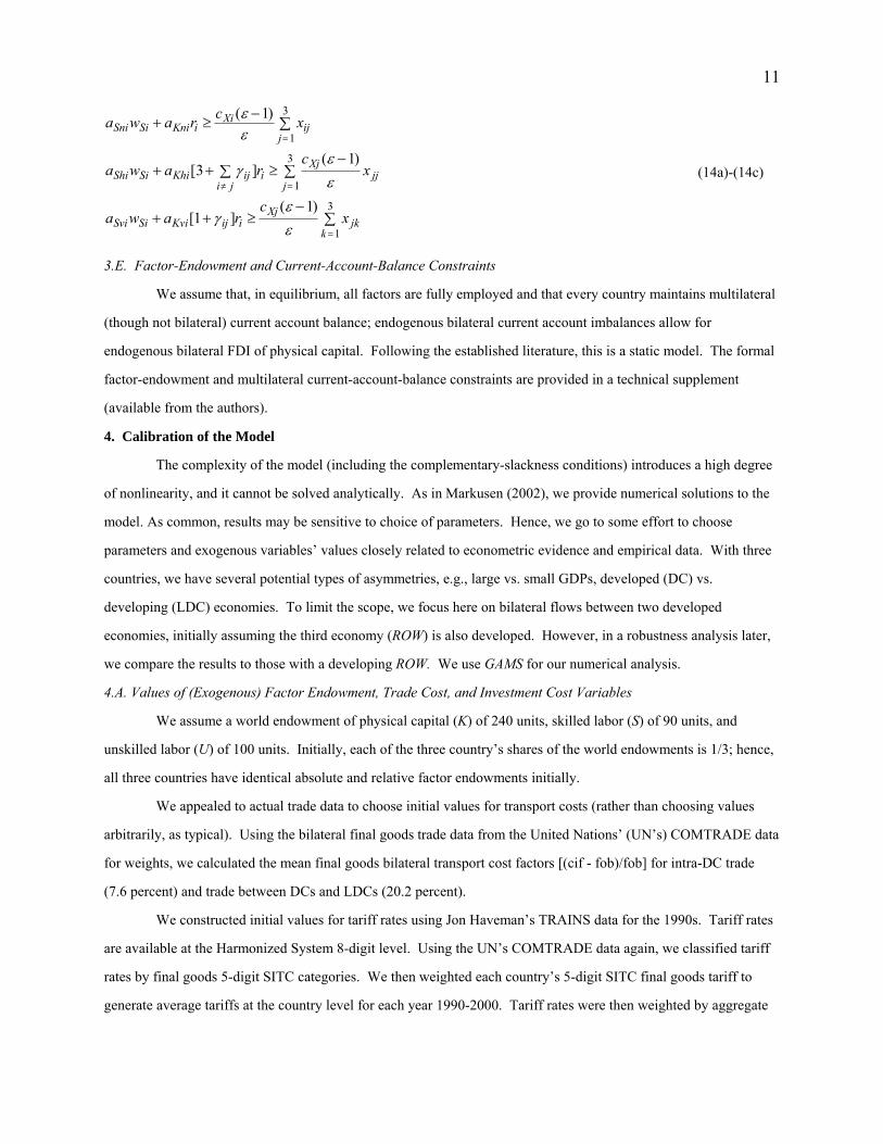
Figures 1a and 1b illustrate the issue for the 2x2x2 case with no physical capital. First, we explain the

figures’ axes and labeling. Given the nonlinear, nonmonotonic relationships in this class of GE models, we must

rely on numerical solutions to the model to obtain “theoretical” relationships, using figures generated by the

numerical model. In these figures, we focus on the bilateral relationships between two economies with identical

relative factor endowments and transaction cost levels. Figures 1a and 1b illustrate the relationships between

country economic size (referred to as the sum of GDPs of i and j) on the y-axis, similarity of economic size on the x-

axis, and final good exports of NEs from i to j (the values of foreign affiliate sales of country i’s HMNEs in country

j) on the z-axis in Figure 1a (1b).14 The lines on the y-axis in the bottom plane range from 1 to 21. The y-axis

indexes the joint absolute factor endowments of countries i and j; line 1 denotes the smallest combination and line 21

denotes the largest combination. The x-axis is indexed from 0 to 1. Each line represents i’s share of both countries’

absolute factor endowments; the center line represents 50 percent, or identical GDP shares for i and j.15

These figures are three-dimensional analogues to a two-dimensional figure in Markusen (2002, p. 99,

Figure 5.5, bottom). Our figures allow a range of total economic sizes for the two countries, whereas Markusen’s

14

16Of course, in the two-country case, the sum of GDPs of i and j is world GDP. However, to maintainconsistent labeling of axes with the three-country case later, we label the y axis with sum of GDPs of i and j.

17Shin (2005) used this assumption to motivate exogenously coexistence of MNEs and NEs.

corresponding figure was for a (single) given total economic size for the two countries.16 Suppose initially that

country j has the smallest possible GDP (i.e., virtually no factor endowments) and country i has virtually all of the

two countries’ endowments; this is the first point on the far RHS of Figures 1a and 1b. When country j is very small,

it is most profitably served by the only other country, i, by national firms exporting from i; hence, HMNEs based in i

will not serve j with foreign affiliate sales (FASij=0). Even a slightly larger GDP in country j (the point to the left of

the initial one) is not enough to make human capital sufficiently scarce to warrant FAS. However, at higher levels

(moving to the left), country j is a large enough market to warrant foreign affiliate production by country i given

investment barriers, and exports by national firms in i are partially “displaced” by the scarcity of human capital. At

equal GDPs, HMNEs displace trade completely (FASij > 0 and trade is zero).

The complete displacement of trade in the 2x2x2 model was formalized in Markusen and Venables (2000,

section 4). More accurately, in their model there exists only a (highly unlikely) unique combination of trade costs (t)

and ratio of national-to-multinational-firm setup costs (f/g) where HMNEs and NEs can coexist when the two

countries are symmetric and the equilibrium is in the factor-price-equalization set (where mill prices and marginal

production costs are equal). In the two-factor case, only if f/g is chosen to equal precisely (1+ t1-ε)/2 can NEs and

HMNEs coexist, where ε is the elasticity of substitution between varieties in their model.17

A resolution to this puzzle lies readily in introducing a third internationally-mobile factor and an

assumption that home physical (human) capital is used to set up a plant (firm). The introduction of physical capital

and the setup requirements can explain the observed coexistence of final goods trade (NEs) and FAS (HMNEs) when

the two countries’ GDPs are identical for a wide range of parameters. In simulations below, ROW has zero factor

endowments; conclusions result solely from introducing physical capital and the setup requirements.

Figures 2a-2c illustrate the implications for foreign affiliate sales, trade, and horizontal foreign direct

investment, respectively, between a pair of developed countries (i,j) with identical relative factor endowments in our

three-factor, two-country, two-good world. The most important point worth noting is that, when the two countries

have identical GDPs, NEs and HMNEs can coexist. However, similar to the 2x2x2 world, once HMNEs arise, FAS

tends to partially displace trade and national exporters no matter how large are the GDPs of countries i and j, cf.,

middle columns in Figures 2a and 2b. The intuition can be seen by starting at the far right side of Figure 2b, when

j’s GDP is small relative to i’s. When j’s GDP share becomes positive (via an exogenous reallocation of initial factor

endowments from i to j), j’s relatively small market is most profitably served by exports from national firms in i and

domestic production in j, identical to the 2x2x2 case. Thus, i exports extensively to j.

15

18Recall, human and physical capital are complements in production of differentiated goods, not in setups.

As j’s (i’s) share of their combined GDPs gets larger (smaller), the number of exporters and varieties in i

(ni) contracts, cf, Figure 3a. However, output per firm in j (xjj, not shown), production, and overall demand expands

proportionately more, such that exports from i to j increase, cf., Figure 2b.

At some point (around 0.7 on the x-axis), as i’s (j’s) share gets even smaller (larger), it becomes more

profitable for i to serve j’s market using HMNEs (h2ij) to avoid trade costs, cf., Figure 3b. So FDI – physical capital

– flows from i to j, so that both countries’ markets can be more efficiently served by HMNEs based in i, cf., Figure

2c. In the two-factor case with only human capital used to set up plants and firms, this would unambiguously

increase the price of skilled (relative to unskilled) labor, displacing completely national firms in i. This need not

occur here. While the replacement of NEs by MNEs requires more human capital for firm setups (as in the 2x2x2

model), the net demand for human capital in i goes down because in our model plant setups require only physical

capital. Since single-plant NEs are being increasingly replaced by multi-plant HMNEs as i and j become more

similar in size (note the “dip” in the center columns of Figure 3a when i’s and j’s shares are very similar), the

relative demand for human capital falls and that for physical capital rises, lowering (raising) the price of human

(physical) capital, cf., Figures 3c and 3d.18 This has two important implications for NEs not being completely

displaced, and thus coexistence of NEs and HMNEs when i and j are identical. First, a higher price of physical

capital in i (as i and j converge in size) raises the relative price of multi-plant HMNE firm setups, reducing the

displacement of single-plant national firms (which serve markets via exports instead) and helping secure their

coexistence with HMNEs. Second, a lower price of human capital in i lowers the price of HMNE and NE firm

setups, also securing coexistence of both types of firms. As j’s share approaches that of i, HMNEs continue to

partially displace national firms. However, even with identical GDPs, HMNEs and national firms can coexist–a

result precluded in the 2x2x2 model.

With physical capital, coexistence of HMNEs and NEs occurs over a wide range of economic sizes, GDP

similarities, plant-to-firm setup costs, and trade costs, because of variable relative prices of human-to-physical

capital, cf., Figures 3c and 3d. We now demonstrate formally such coexistence for a wide parameter range.

Consider the case of two symmetric economies where mill prices of the countries’ differentiated products are

identical (pXi = pXj), as in Markusen and Venables (2000, section 4). Begin with profit functions (12) from section

3.D. With only two countries, there are no three-country HMNEs; we will have two-country HMNEs in equilibrium

(h2). With two symmetric economies in size and relative factor endowments, there are no vertical MNEs (v). Hence,

in equilibrium, zero profits ensure for the representative firm in i (and symmetrically in j):

(15a-15b)π

π γn X X ii ij Sn S Kn

h Xi Xi ii X X jj Sh S Kh

p c x x a w a r

p c x p c x a w a r

= − + − − =

= − + − − − + =

( )( )

( ) ( ) [ ]

0

2 02 2 2

16

19We can also show that the addition of the third factor alone is not sufficient to ensure coexistence. Eliminating the physical capital requirement in plant setup costs (replacing it with human capital) leads to a unique-solution result, as in Markusen and Venables (2000). However, it is not critical that physical (human) capital is usedfor plant (firm) setups; this assumption can be reversed, as long as the world endowment of skilled labor is increased(to ensure positive FDI and FAS).

Since mill prices are the same in i and j, we can use equation (9) to note:

(16)xx

t bijX X= +− −1 11σ ( )

where, due to symmetry, x = xii = xjj.

We can now solve for the necessary condition that ensures coexistence of NEs and HMNEs.

Substituting equation (16) into equation (15a) and solving for (pX - cX)x yields:

( ) ( ) / [ ( ) ]p c x a w a r t bX X Sn S Kn X X− = + + +− −1 11 1σ

However, we know from equation (15b) that:

2 22 2( ) ( [ ] )p c x a w a rX X Sh S Kh− = + + γ

Hence, after some algebra, the necessary condition for coexistence is:

[( ( / ) ( )] / [ ( / ) ] / [ ( ) ]a w r a a w r a t bSh S Kh Sn S Kn X X2 2

1 12 2 1 1+ + = + + +− −γ σ

Thus, unlike in Markusen and Venables (2000), NEs and HMNEs can coexist for two identically-sized economies

across a wide variety of values of trade costs, investment costs, and plant-to-firm setup costs due to the endogeneity

of the relative price of human-to-physical capital.19

As in this class of models, the results are, of course, sensitive quantitatively to levels of transport costs,

investment costs, firm fixed costs, and plant fixed costs. However, these results hold for a wide range of values.

Although the presence of physical capital and the assumption that plant setups use only physical capital generate the

result that horizontal MNEs need not displace trade completely, the degree of substitutability or complementarity of

bilateral trade and FDI with respect to economic size and similarity depends upon the presence of a “third country.”

6. Complementarity: The Three-Country, Three-Factor Case

While the gravity equation is familiar in algebraic form, it will be useful to visualize the frictionless

“gravity” relationship. Figure 4a illustrates the gravity-equation relationship between bilateral trade flows, GDP size,

and GDP similarity summarized in equation (3) for an arbitrary hypothetical set of country GDPs (N>2). Of course,

one notes a qualitative similarity of Figure 4a to Figures 2a-2c.

However, there are (at least) three notable shortcomings that the two-country model cannot address. First,

Figures 2a-2c represent bilateral and multilateral international flows; these figures depict a two-country world. With

only two countries one cannot identify the effect of ROW on the bilateral flow from i to j; a theoretical foundation

17

20In the center cell of the x- and y-axes of Figures 4 and 5, all three countries’ GDPs are identical.

for the bilateral gravity equation needs at least three countries.

Second, with two countries the trade flow from i to j is non-monotonic in GDP similarity, cf., Figure 2b. In

a gravity equation, the trade flow is monotonic in economic similarity, cf., Figure 4a. This conflicts with empirical

results of trade and FDI gravity equations that imply bilateral trade and FDI are complements with respect to GDP

size and similarity.

Third, in contrast to trade gravity equations, typical FDI gravity equation estimates find home country GDP

elasticities significantly larger than host country GDP elasticities, cf., Table 1. This asymmetry cannot be explained

using the two-country, three-factor model, cf., Figure 2c.

In part A, we address these three shortcomings. First, we explain why the introduction of a third country is

necessary to generate “complementary” relationships between two countries’ bilateral trade, FDI, and FAS flows

with the two countries’ GDP size and similarity. We address why the numbers of NEs and HMNEs also change in a

complementary way with respect to changes in the two countries’ economic size and similarity – even though NEs

and HMNEs remain “overall” substitutes. Moreover, by introducing the third country, we can explain readily why

typical empirical FDI gravity equations find home country (i) GDP elasticities significantly larger than host country

(j) GDP elasticities. In part B, we show the explicit relationship between size of the third country’s (ROW’s) GDP

and trade, FDI and FAS of countries i and j, and suggest some “testable” hypotheses about the relationships between

trade from i to j and FDI from i to j with GDPROW.

6.A. A Theoretical Rationale for Estimating Gravity Equations of Trade, FAS, and FDI

In this section, we introduce a third country – ROW – which initially is identical to the other two countries;

the three countries are referred to as i, j, and ROW. Figures 4b-4d (5a-5d) are the analogous “three-country” figures

to two-country Figures 2a-2c (3a-3d).20 First, we note unsurprisingly in Figures 4b-4d that bilateral FAS, trade, and

FDI from i to j, respectively (henceforth, FASij, Tradeij, and FDIij) are all positive monotonic functions of the size of

the two countries’ GDPs for any given share of i in i’s and j’s total GDP, as the gravity equation suggests (cf., Figure

4a) for a given GDPROW. Note in Figures 5a and 5b that the numbers of both NEs and HMNEs increase with a larger

joint economic size. More resources cover more setup costs of NEs and HMNEs; economies of scale and love of

variety expand the number of total varieties produced for all three countries by both types of firms in i.

Second, and more interesting, even though NEs and HMNEs remain substitutes overall, the presence of the

third country allows both bilateral FAS and trade from i to j to reach maximums as these two countries converge in

GDP size, as a gravity equation would suggest; unlike the two-country case, FASij and Tradeij are “complements”

with respect to similarity in i’s and j’s GDPs. Note first that Figures 4b and 4c (5a and 5b) illustrate that FASij and

Tradeij (NEs and HMNEs in i) remain substitutes overall. For any given size and similarity, the number of HMNEs

18

21For instance, as j’s share of i’s and j’s GDPs goes from 0 to ½ (for the smallest sum of GDPs of i and j),the fall in the price of i’s human capital is 7.8 (1.2) percent for the three- (two-) country case and the rise in the priceof i’s physical capital is 16.7 (2.0) percent for the three- (two-) country case.

(NEs) is larger (smaller) in the 3-country world than in the 2-country world; compare any cell in Figure 5b (5a) with

the corresponding cell in Figure 3b (3a). Enlarging the world’s economic size shifts the structure of all three

economies toward relatively more HMNEs and fewer NEs; in this dimension, NEs and HMNEs are “overall”

substitutes. With three countries, HMNEs surface more readily to avoid expensive trade costs; i can more profitably

serve j and ROW by avoiding trade costs and investing in plants abroad. Note in Figure 5b (4d) that i’s number of

three-country HMNEs (i’s bilateral FDI from i to j) is positive even when j’s GDP is quite small relative to i’s.

FASij and FDIij (Tradeij) is larger (smaller) in the 3-country relative to 2-country world. The overall substitution of

FAS and FDI for trade also explains the “flattening” of the FAS (FDI) theoretical surface in Figure 4b (4d) relative

to that in Figure 2a (2c); with more HMNEs in the 3-country world, FAS spreads out over a wider range of GDPs

sizes and similarities since FDI occurs even when j’s GDP is small.

Yet, if the presence of a third country causes FASij to tend to substitute more for Tradeij for any given level

of GDP size and similarity, why do both increase as the country pair’s GDPs become more identical with three

countries but not with two? As the GDPs of countries i and j become more identical, Figures 5c and 5d illustrate that

the price of human (physical) capital tends to fall (rise). However, the larger percentage fall (rise) in the price of

human (physical) capital with three countries than with two dampens the increase in HMNEs and the decrease in

NEs more with three countries.21 The dampening of the increase in the number of HMNEs contributes to

“flattening” the FAS and FDI surfaces with three countries compared with two. The dampening of the decrease in

the number of NEs is sufficient to cause Tradeij to be monotonic in size and similarity of the GDPs of countries i and

j in the three-country case. The combined effect is to cause FASij and Tradeij to – on net – covary positively and

monotonically with respect to country i’s and j’s GDP size and similarity in the three-country world. This is the

main economic reason behind the gravity equation working for FAS, FDI, and trade flows simultaneously!

Consequently, i’s FAS in j and trade from i to j are maximized when these two countries have identical

GDPs (Figures 4b and 4c), as a result of a third country and third factor. Thus, the theoretical relationships between

bilateral trade, FDI, and FAS flows and GDPs in Figures 4b-4d are “well approximated” by the gravity relationship.

However, note that the theoretical surface for FDI in Figure 4d is distinctly asymmetric relative to the other surfaces.

FDI from i to j is maximized when i’s share of the two countries’ GDPs is larger than j’s share. It can be shown

mathematically that such a surface implies the home country GDP elasticity of FDI has to be larger than the host

country GDP elasticity. Thus, with three countries one should expect the empirical result found in specification (3)

in Table 1, that is, a larger home country (i) GDP elasticity than host country (j) GDP elasticity for FDIij.

However, “eyeballing” surfaces 4c and 4d cannot explain the empirical results using (the more

19

econometrically appropriate) fixed effects results in specifications (5)-(8) in Table 1. In section 7 we move beyond

“ocular-metrics” to provide a quantitative theoretical rationale for GDP elasticities estimated using fixed effects.

6.B. The Effect of ROW on Bilateral Trade

In this part, we motivate potentially “testable” propositions about the empirical correlations between FDIij

and GDPROW and between Tradeij and GDPROW. Figures 6a-6c show the relationships between the ROW’s GDP (x-

axis), the combined GDPs of i and j (y-axis), and Tradeij, FASij, and FDIij, respectively (z-axis). Here, the GDPs of

countries i and j are set to be identical to each other, but their combined GDPs can vary. The cell in the middle row

of the first column is defined to be identical absolute (and relative) factor endowments for countries i, j and ROW.

Suppose all three countries have identical absolute factor endowments; when countries i and j have two-thirds of the

world’s GDP (for which there is no empirical counterpart, as will be shown), an increase in ROW’s GDP makes FDIij

relatively more attractive and Tradeij less attractive. As ROW’s size initially increases, the profitability in country i

from having more three-country HMNEs rises to avoid expensive transport costs to either j or ROW; hence, FDI

from i to j (as well as i to ROW) increases, substituting for exports from i to j (Tradeij falls). However, as ROW

continues to increase in economic size (moving to the right along the middle row of the x-y plane), the relative

market sizes of i and j shrink, attracting less exports from i to j by NEs and countries i and j become less attractive

markets in size to be served efficiently by HMNEs in i and j.

The model suggests two potentially “testable” hypotheses. First, Tradeij should decrease monotonically as

ROW’s GDP increases, consistent with previous formal theoretical models for the trade gravity equation ignoring

MNEs and FDI. Second, the model suggests a quadratic relationship between FDIij and GDPROW; this hypothesis is

novel. Clearly, a positive or negative relationship depends on relative GDPs of i, j, and ROW.

However, examination of actual GDPs suggests the likely relationship to dominate empirically for the

second hypothesis is negative. Recall first that the x-axis has 21 columns. In Figure 6c, GDPROW ranges from the

same size as i (or j) in column 1 to 10 times GDPi (or GDPj) in column 21. Thus, column 2 represents GDPROW =

1.5*GDPi and column 3 represents GDPROW = 2*GDPi, or GDPROW = GDPi + GDPj. Thus, the model hypothesizes

that FDIij and GDPROW should be negatively (positively) correlated for observations where GDPi + GDPj < GDPROW

(GDPi + GDPj > GDPROW).

Does GDP data provide any guidance on the relevant hypothesis? For the last year of our sample (2000),

the combined nominal GDP of the two largest economies in the world – the United States and Japan – was US$14.52

trillion; this was less than half of world GDP ($31.43 trillion, using the 160 largest economies) and hence less than

GDPROW (US$16.91 trillion). Consequently, all empirical observations lie in the negatively-sloped region of Figure

6c. Thus, the model implies two “testable” propositions: Tradeij and FDIij should both be negatively related to ROW

GDP. We evaluate these later empirically.

7. A Quantitative Description of the Theoretical Gravity Equations of Trade and FDI

20

22The diversity of quantitative gravity relationships reflects the model’s “unconditional” GE structure, i.e.,non-separability of production, consumption, trade and FDI allocations. This differs from a standard gravityequation, such as equation (1), which is consistent with the “conditional” GE structure emphasized in Anderson andvan Wincoop (2004, pp. 706-707), which employs a critical “trade-separability” assumption, resulting in unit GDPelasticities. See also footnote 4.

23GDPs are, of course, an endogenous variable. The exogenous variables are the absolute endowments ofunskilled labor, skilled labor, and physical capital. Simulations using these variables yield similar outcomes.

The diversity of gravity-like relationships in specifications (5)-(8) in Table 1 suggests a need for a more

quantitative “description” of the theoretical relationships in Figures 4c and 4d.22 To move beyond “ocular-metrics,”

in part A we describe a new methodology to describe quantitatively the relationship between each of the “theoretical

flows” and the exogenous RHS variables, similar to how a regression describes empirical relationships. In part B,

we present the results of these exercises for describing the theoretical relationships between GDP size, GDP

similarity, and the various flows, and compare these to the empirical results in Table 1. In part C, we use the

numerical GE model to illustrate theoretical relationships between trade costs, investment costs, RTAs, trade flows,

and FDI. In part D, we use data on ROW GDP and bilateral trade and investment costs to extend empirical results to

determine if the “testable” propositions regarding ROW GDP, trade costs, investment costs, and trade and FDI flows

hold. In part E, we discuss some sensitivity analyses that were conducted.

7.A. Methodology

The key notion behind the methodology that follows is to describe quantitatively using a single regression

equation a nonlinear theoretical surface relating bilateral flows to GDP size and similarity generated by a numerical

GE model. We have empirical data on GDP sizes and similarities. Our surfaces map certain “theoretical” levels of

bilateral (trade, FDI, or FAS) flows to various GDP sizes and similarities. However, since it is a nonlinear surface,

there is an “approximation error” relating the level of the flow to GDP sizes and similarities. We treat this error term

as normally distributed (and can confirm that assumption) so that a regression of the “theoretical” flow on GDP sizes

and similarities describes the surface quantitatively.

Our methodology using regressions on “theoretical” flows is described most transparently using several

steps. First, consider the bottom plane in Figure 4c. The x-axis indexes country i’s share of i’s and j’s total GDP,

ranging from 0 to 1. The y-axis represents the sum of GDPs of countries i and j (GDPT).23 The x- (y-) axis actually

consists of 99 columns (600 rows); however, if we had used 99 columns (600 rows) in Figure 4c, the entire figure

would be black due to too many lines on the grid. For readability, the figures shown aggregate the 99 columns (600

rows) into 21 columns and rows so each cell’s color content is visible. On the y-axis, the initial level of the country

pair’s GDP sum is set to one. The next line’s GDP sum is six percent larger than the first line’s GDP, the third line’s

GDP sum is six percent larger than the second line’s GDP, and so on for 600 entries. Thus, GDP sums vary from 1

to (approximately) 37. This generates 59,400 (=99x600) cells with “theoretical” observations on (i’s and j’s) GDP

21

24We could have even added a stochastic error term explicitly; this would not have changed our results.

25Not every one of the 59,400 theoretical cells will be used. Also, we exclude all zero theoretical flows. The only difference between our regressions and typical regression analysis using empirical data on both sides of theregression is that the LHS variable is from the theoretical surface; RHS variables are random variables and the errorterm is normally distributed. Note, we are not testing the theory; we are simply describing the theory quantitatively.

sums, GDP shares, and the level of trade flow, FDI, or FAS implied by the model.

We could run a regression of the numerical GE model’s estimates of the (log) levels of the theoretical trade

flows from i to j on (logs of) i’s and j’s GDP sum and similarity (Ei + Ej and sisj, respectively) using each “cell” once

as an observation, similar to Figure 4a. The “error terms” would be the approximation (or rounding) errors

generated from the nonlinearity of the surface and behave as if randomly distributed.24 However, running such a

regression would have limited economic meaning since each cell has the same weight in the distribution. Some of

the cells (in terms of GDP totals and similarity) might not even be observed empirically!

Consequently, we create a more relevant distribution for the cells by benchmarking the (bottom) plane to

empirical data on GDPs from World Development Indicators. We then fill each cell based upon observations of

GDP sums and i’s share of their GDP for that cell; that is, we “match” theoretical values of GDP size and similarity

to their empirical observations for each country pair. Using our sample of the 17 most developed OECD countries’

annual GDPs for 1990-2000, we fill the cells with the observations corresponding to each country pair with a certain

GDP sum and GDP share (i’s share of the GDP of i and j). For example, along the x-axis the first column includes

all observations in the panel for which i’s GDP share is between 0 and (approximately) 1 percent of a country pair’s

total GDP (recall, there are actually 99 columns). Along the y-axis, the first row (of actually 600 rows) includes all

observations in the panel for which the GDP sum is smallest and up to 6 percent higher than that. The largest GDP

sum in the sample (i.e., U.S.-Japan GDP sum for year 2000) amounts to about 37 times that of the smallest country

pair. Thus, we have created a distribution of frequencies of cells based upon GDP sums and similarities using cross-

section and time-series data. We then estimate the regression relationship between the theoretical value for a

country pair’s flow from i to j (using separately each of the three flows) based upon the model with the values for the

GDP sums and i’s GDP shares based on actual GDP data.25

7.B. Regression Results using Theoretical Flows

Specifications (9)-(12) in Table 1 are the results of running the regressions using “theoretical” flows from i

to j. Specification (9) reveals that theoretical trade flows from i to j are positively related to the countries’ GDPs.

The results are qualitatively identical to those in fixed-effects specification (5) in Table 1 using actual trade flows.

The exporter GDP elasticity is smaller than the importer GDP elasticity in both specifications. A comparison of

specification (10) using theoretical flows with fixed-effects specification (6) using actual trade flows shows that the

results are qualitatively similar for GDP size and similarity. GDP similarity elasticities are nearly the same.

22

26The relationships shown in Figures 7a and 7b are for the case of three countries that are identical inabsolute and relative factor endowments, as in Markusen (2002, sections 5.5). If relative factor endowments wereallowed to differ, such as in Markusen (2002, sections 8.5 and 8.6), we would obtain nonmonotonic relationships. However, our purpose in Figures 7a and 7b is to motivate expected empirical relationships for trade and FDI flowswith trade and investment costs in the context of an empirical gravity equation where the interaction of such costsand relative factor endowments is assumed to be minimized by the logarithmic transformation.

Specifications (11) and (12) in Table 1 report the coefficient estimates using the analogous specifications

for “theoretical” FDI flows. Notably, the home country GDP elasticity is larger than the host country GDP elasticity

in specification (11), consistent with fixed-effects specification (7) using actual FDI flows. Moreover, the GDP

similarity elasticity in specification (12) is comparable to that in specification (8) using actual FDI flows. However,

the GDP size elasticities are much larger in specifications (6) and (8) using empirical trade and FDI flows than in

corresponding specifications (10) and (12) using theoretical flows. The relatively high GDP size elasticities may be

sensitive to omitted variables or the particular period used for empirics (1990-2000); our time series was constrained

by bilateral trade and investment cost data availability. We address potential omitted variables bias in part D.

7.C. Effects of Trade and Investment Costs, Regional Trade Agreements, and Relative Factor Endowments

Of course, one of the most important variables in any trade or FDI gravity equation is bilateral distance,

typically included as a proxy for trade or investment costs, respectively. Both trade and investment costs are

included explicitly in our theoretical model (as in Markusen, 2002). Figure 7a (7b) shows the relationship between

bilateral trade (FDI) flows, trade costs, and investments costs in our model. As expected, Tradeij (FDIij) is negatively

related to trade (investment) costs between i and j. Moreover, the model suggests, as common in this literature, that

Tradeij (FDIij) is positively related to investment (trade) costs between i and j. These “testable” propositions are

evaluated empirically later.26

Figures 7c and 7d illustrate the effect of introducing a bilateral regional free trade agreement (RTA)

between countries i and j in our three-country model. The theory suggests that a reduction in bilateral trade costs is

associated with a higher level of bilateral trade, cf., Figure 7c. However, a reduction in trade costs makes bilateral

investment less economical, and should tend to reduce bilateral FDI,cf., McCulloch (1985,1993). Figure 7d confirms

that the model suggests that a free trade agreement between i and j should be associated with a lower level of

bilateral investment from i to j. (Figures 7c-7d also provide a theoretical rationale for the multiplicative relationships

between measures of trade and investment costs, GDPs, and trade and FDI flows in typical gravity equations.) In

section 7D, we evaluate empirically whether trade (investment) is positively (negatively) related to RTA.

Up to now, countries have had identical relative factor endowments. In the interest of robustness, we

allowed ROW to be a developing country by having a larger (smaller) initial share of the world’s unskilled labor

(human and physical capital). With this change, vertical MNEs surface. However, the results are largely robust to

this change. The surfaces examined in Figures 4-7 are qualitatively (not quantitatively) identical with a developed or

23

developing ROW; figures are omitted due to space constraints.

Also, our theoretical surfaces assume countries i and j have identical relative factor endowments. As

discussed in Carr, Markusen, and Maskus (2001), Blonigen, Davies, and Head (2003), and Braconier, Norback, and

Urban (2005), theoretical relationships between relative factor endowments of countries i and j and trade, FAS, and

FDI flows from i to j are interesting as well. However, examining those theoretical relationships for our three-factor

model is well beyond the scope of this paper and the subject of future research. Nevertheless, even developed

country pairs are likely to have different relative factor endowments. To ensure the empirical results that follow

account for variation in relative factor endowments between i and j, we include relative factor endowments of

country pairs.

7.D. Final Empirical Results

The previous sections suggest three potentially “testable” propositions that can be investigated empirically

using time-series (within) variation. First, section 5B suggested Tradeijt should be negatively related to GDPROW and

– based upon the actual size distribution of the world’s GDPs – FDIijt should also be related negatively to GDPROW.

Second, section 6C suggested Tradeijt (FDIijt) should be negatively related to bilateral trade (investment) costs and

positively related to bilateral investment (trade) costs. Third, section 6C suggested Tradeijt (FDIijt) should be

positively (negatively) related to an RTA dummy.

Specifications (13)-(16) in Table 1 report the results using bilateral fixed effects of estimating the same

specifications similar to (5)-(8) but now adding ROW GDP, bilateral trade (cif-fob) and investment costs, and

relative factor endowments of countries i and j. Trade and investment costs data were described in section 4; factor

endowment data are from Baier, Dwyer and Tamura (2004). First, we find that Tradeij and FDIij are both statistically

significantly negatively related to GDPROW as expected. Second, we find that Tradeij (FDIij) is negatively related to

bilateral trade (investment) costs as expected and the coefficient estimate is statistically significant at the 10 percent

level (two-tailed t-tests). The relationship between Tradeij (FDIij) and bilateral investment (trade) costs is not

correctly signed, but these cross-price elasticities are much smaller than the own-price elasticities. Third, due to our

data set (which was limited by investment cost data), we have no time-series variation in the free trade agreement

dummy variable. However, we do have cross-section variation. A reexamination of Table 1's empirical gravity

equation coefficient estimates for the dummy variable representing a free trade agreement (=1 if RTA present, = 0

otherwise) using panel data in specifications (1)-(4) shows that a reduction in “trade costs” (in the form of the

presence of a free trade agreement) is correlated with a higher level of bilateral trade – but a lower level of bilateral

investment – between a pair of countries, consistent with our theory. Finally, while theoretical predictions for the

relationships between relative factor endowments of country i relative to j on flows are beyond the scope of this

paper, we find that FDIij is positively and statistically significantly related to the (log) physical-capital-to-unskilled-

labor (K/U) ratios (in i relative to j) and the (log) human-capital-to-unskilled-labor (S/U) ratios. Tradeij is negatively

24

related to the relative K/U ratios, but is positively and statistically significantly related to the relative S/U ratios.

7.E. Sensitivity of Results to Parameter Selections and Exogenous Variables

Of course, the potential number of alternative calibrations of our numerical GE model is virtually unlimited.

Paper space constraints prevent an exhaustive analysis of permutations from our base calibration. Nevertheless, we

evaluated the sensitivity of the model’s theoretical surfaces to assuming setups of headquarters (plants) require

human (physical) capital and to varying trade-relative-to-investment costs, MNE/NE ratio firm setup costs, the

capital-skill elasticity of technical substitution, and the elasticity of substitution of differentiated goods in utility. A

complete discussion of these findings is in a technical supplement (at http://www.nd.edu/~jbergstr).

8. Conclusions and Directions for Future Research

The introduction of a third internationally-mobile factor to the standard 2x2x2 model allows us to resolve

fairly readily a puzzle in the modern knowledge-capital literature on MNEs (without heterogeneous productivities

among firms) that foreign affiliate sales among two identical economies completely displace their intra-industry

trade. The introduction of a third country suggests a formal N-country theoretical rationale for estimating gravity

equations of FDI flows and foreign affiliate sales, in a manner consistent with estimating trade gravity equations.

Our future research agenda is quite large. We intend to extend our methodological framework to examine

theoretically the economic determinants of trade, FDI, and FAS flows between developed and developing countries,

and among developing countries. We plan to incorporate intermediate goods to better understand the role of

“outsourcing” for NEs and MNEs. We intend to investigate further the role of physical capital for better

understanding the empirical relationships between relative factor endowments and the pattern of MNE behavior as

raised in Carr, Markusen, and Maskus (2001) and Blonigen, Davies, and Head (2003).

REFERENCES

Anderson, James E., and van Wincoop, Eric. “Gravity with Gravitas: A Solution to the Border Puzzle.” AmericanEconomic Review 93, no. 1 (March 2003): 170-192.

Anderson, James E., and van Wincoop, Eric. “Trade Costs.” Journal of Economic Literature 42, no. 3, September2004, 691-751.

Baier, Scott L., and Bergstrand, Jeffrey H. “The Growth of World Trade: Tariffs, Transport Costs, and IncomeSimilarity.” Journal of International Economics 53, no. 1, February 2001, 1-27.

Baier, Scott L., and Bergstrand, Jeffrey H. “Do Free Trade Agreements Actually Increase Members’ InternationalTrade?” Journal of International Economics 71, no. 1, February 2007, 72-95.

Baier, Scott L., Dwyer, Gerald, and Tamura, Robert. “How Important are Capital and Total Factor Productivity forEconomic Growth?” Economic Inquiry 44, no. 1, January 2004, 23-49.

Baldwin, Richard E., and Ottaviano, Gianmarco. “Multiproduct Multinationals and Reciprocal FDI Dumping.” Journal of International Economics 54, no. , 2001, 429-448.

Barba Navaretti, G., and Venables, Anthony J. Multinational Firms in the World Economy, Princeton, NJ:

25

Princeton University Press, forthcoming 2004.

Bergstrand, Jeffrey H., and Egger, Peter. “A Theoretical and Empirical Model of International Trade and ForeignDirect Investment with Outsourcing: Part I, Developed Countries.” Working paper, April 2004.

Bergstrand, Jeffrey H., and Egger, Peter. “A Knowledge-and-Physical-Capital Model of International Trade,Foreign Direct Investment, and Foreign Affiliate Sales: Developed Countries.” Working paper, Jan. 2006.

Blonigen, Bruce A. “In Search of Substitution between Foreign Production and Exports.” Journal of InternationalEconomics 53, no. 1, February 2001, 81-104.

Blonigen, Bruce A. “A Review of the Empirical Literature on FDI Determinants.” Manuscript, 2005.

Blonigen, Bruce A., Davies, Ronald B., and Head, Keith. “Estimating the Knowledge-Capital Model of theMultinational Enterprise: Comment.” American Economic Review 93, no. 3, 2003, 980-994.

Blonigen, Bruce A., Davies, Ronald B., Waddell, Glen R., and Naughton, H. “FDI in Space.” Working paper,University of Oregon, August 2004.

Borga, Maria, and Yorgason, Daniel R. “Direct Investment Positions for 2001: Country and Industry Detail.” Survey of Current Business, U.S. Department of Commerce, July 2002, 25-35.

Braconier, Henrik, Norback, Pehr-Johan, and Urban, Dieter. “Reconciling the Evidence on the Knowledge-CapitalModel.” Review of International Economics 13, no. 4, September 2005, 770-786.

Carr, David, Markusen, James R., and Maskus, Keith E. “Estimating the Knowledge-Capital Model of theMultinational Enterprise.” American Economic Review 91, no. 3, June 2001, 693-708.

Ekholm, Karolina, Forslid, Rikard, and Markusen, James R. “Export-Platform Foreign Direct Investment.” Journalof the European Economic Association, forthcoming 2007.

Feenstra, Robert C. Advanced International Trade: Theory and Evidence. Princeton, NJ: Princeton U. Press, 2004.

Frankel, Jeffrey A. Regional Trading Blocs in the World Economic System. Washington, DC: Institute forInternational Economics, 1997.

Goldin, Claudia, and Katz, Lawrence F. “The Origins of Technology-Skill Complementarity.” Quarterly Journal ofEconomics 113, no. 3, 693-732.

Grazalian, Pascal L., and Furtan, W. Hartley. “The Border Effects: Recognizing the Role of FDI.” Working paper,University of Saskatchewan, 2005.

Griliches, Z. “Capital-Skill Complementarity.” Review of Economics and Statistics 51, no. 4, Nov. 1969, 465-468.

Head, Keith, and Ries, John. “Overseas Investment and Firm Exports.” Review of International Economics 9, no. 1,February 2001, 108-122.

Head, Keith, and Ries, John. “Increasing Returns Versus National Product Differentiation as an Explanation for thePattern of U.S-Canada Trade.” American Economic Review 91, no. 4, September 2001, 858-876.

Helpman, Elhanan. “Trade, FDI, and the Organization of Firms.” Journal of Economic Literature 44, no. 3,September 2006, 589-630.

Helpman, Elhanan, and Krugman, Paul. Market Structure and Foreign Trade. Cambridge, MA: MIT Press, 1985.

26

Helpman, Elhanan, Melitz, Marc, and Yeaple, Stephen. “Export versus FDI with Heterogeneous Firms.” AmericanEconomic Review 94, no. 1, March 2004, 300-316.

Kleinert, Jorn, and Toubal, Farid. “Gravity for FDI.” Working paper, Georg-August-Universitat Gottingen, 2005.

Lai, Huiwen, and Zhu, Susan Chun. “U.S. Exports and Multinational Production.” Review of Economics andStatistics 88, no. 3, August 2006, 531-548.

Lipsey, Robert E.. “Home and Host Country Effects of FDI.” NBER Working Paper No. 9293, October 2002.

Markusen, James R. “The Boundaries of Multinational Enterprises and the Theory of International Trade.” Journalof Economic Perspectives 9, no. 2, Spring 1995, 169-189.

Markusen, James R. Multinational Firms and the Theory of International Trade. Cambridge, MA: MIT Press, 2002.

Markusen, James R., and Venables, Anthony J. “The Theory of Endowment, Intra-Industry, and Multi-NationalTrade.” Journal of International Economics 52, December 2000. 209-234.

Martin, Philippe, and Rey, Helene. “Financial Supermarkets: size Matters for Asset Trade.” Journal ofInternational Economics 64, no. 2, December 2004, 335-361.

McCulloch, Rachel. “US Direct Foreign Investment and Trade.” In Asim Erdilek (ed.), Multinationals as MutualInvaders: Intra-Industry Direct Foreign Investment, New York: St. Martin’s Press, 1985, 129-151.

McCulloch, Rachel. “New Perspectives on Foreign Direct Investment.” In Kenneth Froot (ed.), Foreign DirectInvestment, Chicago: University of Chicago Press, 1993, 37-53.

Mundell, Robert. “International Trade and Factor Mobility.” American Economic Review 47, no. 3, 1957, 321-335.

Mutti, John, and Grubert, Harry. “Empirical Asymmetries in Foreign Direct Investment and Taxation.” Journal ofInternational Economics 62, no. 2, March 2004, 337-358.

Shim, Kieun. “Border Effects and FDI: Can FDI Explain the Border Puzzle?” Working paper, U. of Virginia, 2005.

Slaughter, Matthew J. “Production Transfer withing Multinational Enterprises and American Wages.” Journal ofInternational Economics 50, no. 2, April 2000, 449-472.

DATA APPENDIXBilateral trade flow data are from the UN World Trade Database for 1990-2000. Bilateral (outbound) FDI

stock data are from UNCTAD (country profiles) for same years. GDPs are from World Development Indicators(2004). Bilateral distance was computed using “great circle” distances. Dummy variables for adjacency andcommon language are from CEPII (Centre d’Etudes Prospectives et d’Informations Internationales). The 17 OECDcountries include Australia, Austria, Belgium, Canada, Denmark, Finland, France, Germany, Italy, Netherlands,New Zealand, Norway, Sweden, Switzerland, United Kingdom, and United States.

Table 1Coefficient Estimates from Gravity Equations*

Empirical (LHS) Flows, Pooled Cross-Section, Time-Series Data Empirical (LHS) Flows, Bilateral Fixed Effects “Theoretical” Flows for LHS Variables Empirical (LHS) Flows, Bilateral Fixed Effects

(1) (2) (3) (4) (5) (6) (7) (8) (9) (10) (11) (12) (13) (14) (15) (16)RHS Variables ln Tradeijt ln Tradeijt ln FDIijt ln FDIijt ln Tradeijt ln Tradeijt ln FDIijt ln FDIijt ln Tradeijt ln Tradeijt ln FDIijt ln FDIijt ln Tradeijt ln Tradeijt ln FDIijt ln FDIijt

ln GDPit 0.82(86.77)

0.93(39.62)

0.52(5.44)

2.01(5.74)

0.35(89.13)

0.59(36.00)

0.29(2.19)

1.47(12.85)

ln GDPjt 0.80(85.62)

0.78(33.83)

1.51(15.71)

1.39(4.02)

0.58(146.80)

0.21(146.80)

1.04(7.80)

0.73(1.38)

lnGDPTijt 1.62(111.93)

1.78(50.45)

2.07(14.58)

3.45(6.75)

0.99(138.25)

0.95(61.99)

1.36(5.85)

2.11(2.17)

ln GDPSimijt 0.81(38.02)

1.28(25.86)

0.64(5.07)

1.31(2.95)

0.74(83.50)

1.53(75.13)

0.61(4.13)

1.18(2.09)

ln DISTij -0.62(-42.43)

-0.62(-41.09)

-0.84(-24.24)

-0.75(-21.11)

ln LANGij 0.67(19.69)

0.67(19.65)

1.32(16.70)

1.36(17.42)

RTAijt 0.57(14.52)

0.57(14.48)

-0.53(-5.79)

-0.47(-5.17)

ln ROWGDPijt -4.10(-4.86)

-3.80(-3.42)

-9.18(-2.90)

-9.75(2.20)

ln Transport Costsijt -0.02(-5.78)

-0.02(-5.73)

-0.003(-0.21)

-0.003(-0.21)

ln Investment Costsijt -0.004(-2.73)

-0.005(-3.66)

-0.01(-1.94)

-0.01(-1.72)

ln [(S/U)it/(S/U)jt] 1.81(5.35)

1.49(4.47)

5.48(4.18)

5.73(4.43)

ln [(K/U)it/(K/U)jt] -0.07(-0.09)

-0.20(-2.65)

0.56(1.73)

0.67(2.21)

R2 0.87 0.87 0.57 0.58 0.49 0.49 0.33 0.33 0.89 0.86 0.37 0.71 0.51 0.49 0.28 0.27No. of pairs 272 272 266 266 272 272 266 266 272 272 266 266 263 263 254 254No. of observations 2,983 2,983 2,683 2,683 2,983 2,983 2,683 2,683 2,983 2,983 2,683 2,683 2,069 2,069 1,828 1,828

*t-statistics are in parentheses. In empirical regressions, time dummies are included, but coefficient estimates omitted. Bilateral fixed effects’ coefficient estimates are also not reported for brevity. In bilateral fixed effects(empirical) regressions, R2 denotes “Within R2.” All RHS variables use empirical data.

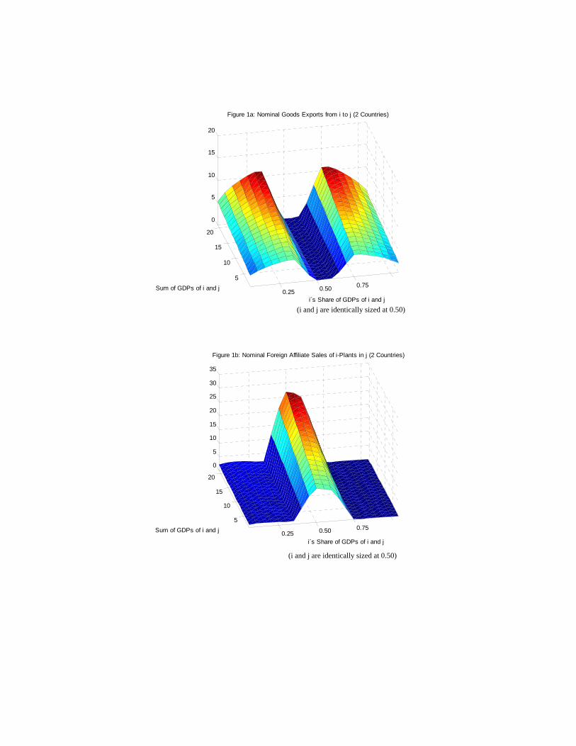
0.25 0.50 0.75

5

10

15

20

0

5

10

15

20

i´s Share of GDPs of i and j

Figure 1a: Nominal Goods Exports from i to j (2 Countries)

Sum of GDPs of i and j

0.25 0.50 0.75

5

10

15

20

0

5

10

15

20

25

30

35

Figure 1b: Nominal Foreign Affiliate Sales of i-Plants in j (2 Countries)

i´s Share of GDPs of i and j

Sum of GDPs of i and j

(i and j are identically sized at 0.50)

(i and j are identically sized at 0.50)

0.25 0.50 0.755

10

15

20

0

0.5

1

1.5

2

2.5

3

Figure 2a: Foreign Affiliate Sales of i`s Plants in j (2 Countries)

i´s Share of GDPs of i and jSum of GDPs of i and j

0.25 0.50 0.75

5

10

15

20

0

5

10

15

20

i´s Share of GDPs of i and j

Figure 2b: Goods Exports from i to j (2 Countries)

Sum of GDPs of i and j

0.25 0.50 0.755

10

15

200

0.02

0.04

0.06

0.08

0.1

i´s Share of GDPs of i and j

Figure 2c: Foreign Direct Investment from i to j (2 Countries)

Sum of GDPs of i and j

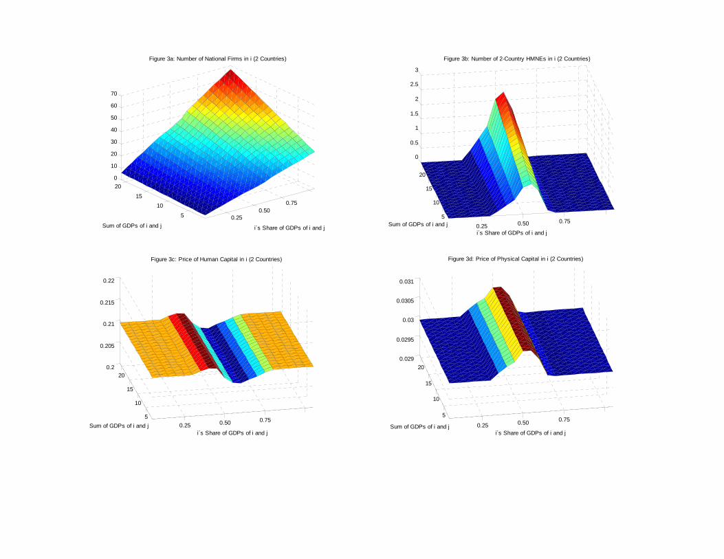
0.25 0.50

0.75

5

1015

200

10

20

30

40

50

60

70

i´s Share of GDPs of i and j

Figure 3a: Number of National Firms in i (2 Countries)

Sum of GDPs of i and j

0.25 0.50 0.75

5

10

15

20

0

0.5

1

1.5

2

2.5

3

Figure 3b: Number of 2-Country HMNEs in i (2 Countries)

i´s Share of GDPs of i and jSum of GDPs of i and j

0.25 0.50 0.755

10

15

200.2

0.205

0.21

0.215

0.22

i´s Share of GDPs of i and j

Figure 3c: Price of Human Capital in i (2 Countries)

Sum of GDPs of i and j

0.25 0.50 0.755

10

15

200.029

0.0295

0.03

0.0305

0.031

i´s Share of GDPs of i and j

Figure 3d: Price of Physical Capital in i (2 Countries)

Sum of GDPs of i and j

0.250.50

0.755

10

15

20

0

10

20

30

40

i´s Share of GDPs of i and j

Figure 4a: Gravity Equation Flow from i to j (3 Countries)

Sum of GDPs of i and j

0.25 0.50 0.75

5

10

15

20

0

2

4

6

8

10

12

Figure 4b: Foreign Affiliate Sales of i`s Plants in j (3 Countries)

i´s Share of GDPs of i and jSum of GDPs of i and j

0.25 0.500.75

5

10

15

20

0

5

10

15

20

25

i´s Share of GDPs of i and j

Figure 4c: Goods Exports from i to j (3 Countries)

Sum of GDPs of i and j

0.25 0.50 0.755

10

15

20

0

0.2

0.4

0.6

0.8

i´s Share of GDPs of i and j

Figure 4d: Foreign Direct Investment from i to j (3 Countries)

Sum of GDPs of i and j

0.250.50

0.75

5

1015

200

10

20

30

40

50

60

70

i´s Share of GDPs of i and j

Figure 5a: Number of National Firms in i (3 Countries)

Sum of GDPs of i and j

0.25 0.50 0.75

5

10

15

20

0

2

4

6

8

10

12

Figure 5b: Number of 3-Country HMNEs in i (3 Countries)

i´s Share of GDPs of i and j

Sum of GDPs of i and j

0.25 0.50 0.755

10

15

20

0.25

0.26

0.27

0.28

0.29

i´s Share of GDPs of i and j

Figure 5c: Price of Human Capital in i (3 Countries)

Sum of GDPs of i and j

0.250.50

0.755

10

15

20

0.04

0.045

0.05

0.055

0.06

i´s Share of GDPs of i and j

Figure 5d: Price of Physical Capital in i (3 Countries)

Sum of GDPs of i and j

510

1520

5

1015

20

4

5

6

7

8

9

GDP of ROW

Figure 6a: Nominal Goods Exports from i to j (3 Countries)

Sum of GDPs of i and j

510

1520

5

1015

20

1

2

3

4

5

GDP of ROW

Figure 6b: Foreign Affiliate Sales of i`s Plants in j (3 Countries)

Sum of GDPs of i and j

510

1520

5

1015

200.05

0.1

0.15

0.2

0.25

0.3

0.35

GDP of ROW

Figure 6c: Foreign Direct Investment from i to j (3 Countries)

Sum of GDPs of i and j

1.0472

1.0487

1.0502

1.0517

0.34

0.39

0.44

0.492.5

3

3.5

4

4.5

Natural trade cost between i and j

Figure 7a: Nominal Goods Exports from i to j (3 Countries)

FDI barrier between i and j

1.04721.0487

1.05021.0517

0.34

0.390.44

0.490.3

0.35

0.4

0.45

0.5

0.55

0.6

Natural trade cost between i and j

Figure 7b: Foreign Direct Investment from i to j (3 Countries)

FDI barrier between i and j

0.250 0.50 0.755

10

15

20

0

0.2

0.4

0.6

0.8

Figure 7c: Change in Level of Nominal Goods Exports from i to j from RTA

i´s Share of GDPs of i and jSum of GDPs of i and j

0.25 0.50 0.755

10

15

20

-0.03

-0.02

-0.01

0

i´s Share of GDPs of i and j

Figure 7d: Change in Level of Foreign Direct Investment from i to j from RTA

Sum of GDPs of i and j