A kinetic model for very low temperature dilute Bose gases ... · We review recent work on a kinetic model ... Keywords low and high temperature quantum kinetics, Bose ... phonon-like

A kinetic model for very low temperature dilute

Bose gases

Linda E. Reichl∗ Minh-Binh Tran†

September 29, 2017

Abstract

We review recent work on a kinetic model for very low temperaturedilute Bose gases. The brief derivation, expressions for hydrodynamicsmodes, and the comparison with a experiment on a BEC of 87Rb atomsare presented.

Keywords low and high temperature quantum kinetics, Bose-Einstein con-densate, quantum Boltzmann equation.

MSC: 82C10, 82C22, 82C40.

Contents

1 Introduction 2

2 The model 3

3 Derivation of the system 63.1 The Kinetic Equation . . . . . . . . . . . . . . . . . . . . . . . . 73.2 Kinetic Equations in Terms of Wigner Functions . . . . . . . . . 93.3 Bogolon Kinetic Equation . . . . . . . . . . . . . . . . . . . . . . 11

4 Microscopic hydrodynamic modes 134.0.1 Zeroth Order Perturbation Theory . . . . . . . . . . . . . 144.0.2 First Order Perturbation Theory . . . . . . . . . . . . . . 154.0.3 Second Order Perturbation Theory . . . . . . . . . . . . . 17

4.1 Comparison to Experiment . . . . . . . . . . . . . . . . . . . . . 19

5 Conclusions 19

6 Acknowledgements 20

∗Department of Physics and Center for Complex Quantum Systems, University of Texas-Austin, Austin, TX 78712, USA. Email: [email protected].†Department of Mathematics, University of Wisconsin-Madison, Madison, WI 53706, USA.

Email: [email protected]

1

arX

iv:1

709.

0998

2v1

[co

nd-m

at.q

uant

-gas

] 2

6 Se

p 20

17

7 Appendix A 20

8 Appendix B 22

9 Appendix C 22

1 Introduction

After the first observation of Bose-Einstein condensation in a gas of rubidium87Rb atoms [3] and then in a gas of sodium 23Na atoms [4], there have been anumber of experiments investigating properties of dilute Bose-Einstein conden-sates (BECs), and it has been shown that the mean field theory of dilute BECs,first proposed by Bogoliubov [5], gives excellent agreement with experiments[9, 26, 36].

If we consider a ideal gas of bosons at temperature T , as the temperatureof the gas is lowered, there is a critical temperature Tc at which a phase transi-tion occurs (Bose-Einstein condensation) and bosons begin to condense into theground state (lowest energy state) of the system. This phase transition also oc-curs for weakly interacting particles like 87Rb and 23Na, which are bosons. Forfinite temperatures T < Tc, the gas can be viewed as a two-fluid system, con-sisting of an irrotational fluid (the condensate) and a normal fluid (the excitedparticles) [6, 39, 40, 47]. The original experiments on BECs confined the atomsto a harmonic optical trap formed by electromagnetic fields. More recently,BECs have also been formed on microelectronic chips [25].

At finite temperatures, the coupling of the condensate and noncondensatedegrees of freedom leads to a two-component condensate-thermal cloud system.The dynamical description of such systems at finite temperature involves a ki-netic equation for the dynamics of thermal excitations coupled to the evolutionequation of the macroscopic phase of the Bose-Einstein condensate. The ther-mal excitations described by Bogoliubov mean field theory can be regarded asa gas of weakly-interacting excitations (“bogolons”), whose energy spectrum isphonon-like at low temperature and particle-like at higher temperatures.

In the pioneering work by Kirkpatrick and Dorfman [31, 32, 33] and Eckern[11], the authors derived a closed kinetic equation for the quasiparticle distribu-tion function of an inhomogeneous Bose gas below the transition temperature.The approach was then employed and extended by Zaremba, Nikuni and Griffin[52]. These theories can be regarded as the consistent time-dependent extensionof the Hartree-Fock-Bogoliubov-Popov theory [37] in which collisions within thethermal cloud and particle-exchange collisions between condensate and thermalatoms are included. Based on a quantum BBGKY hierarchy argument, a similarmodel was also derived in the work [50].

Independently, using a field-theoretic formulation of the non-equilibriumKeldysh theory [7], within the many-body T-matrix approximation, Stoof alsoderived a model [49] that describes the evolution of the full probability distribu-tion for a weakly interacting Bose gas. In this model, using a Hartree-Fock-like

2

ansatz, the total probability distribution can be separated into a product of re-spective probability distributions for the condensate and thermal particles, thatfinally leads to a similar system to the one obtained in [52].

Based on techniques established in the quantum optics community [15], Gar-diner, Zoller and co-workers [12, 30, 13, 29, 14] developed a theory that gives aunified description of the entire range of Bose gas kinetics, combining both co-herent and incoherent processes. Using the above theory, the authors also wrotea different series of papers [18, 17, 16, 34, 8], in which the formation of a BEC inan optical trap was studied. The theories formulated by Stoof [10, 48, 49], andthose formulated by Gardiner-Zoller [12, 13, 14, 29, 30], both have the kineticequations of ZNG as a limiting case. An excellent review of some of these kinetictheories can be found in [41].

All of the above models are based on a picture of excitations with particle-like spectrum. Such models are adequate for high temperature ranges TBEC >T ≥ 0.5TBEC [28], but are inappropriate for describing collective phonon-likeexcitations, which become important at very low temperatures [2]. In order tofix this problem, in [44, 22, 20, 21, 23, 24] authors Reichl and Gust, based on thework of Peletminskii and Yatsenko [38], derived a new kinetic equation whichtakes into account the non-conservation of bogolon number during collisions andthe phonon-like spectrum of bogolons at very low temperature. As a result, anew contribution to the collision operator G31 appears that takes into account1↔3 type collisions between the excitations, addition to the 1↔2 and 2↔2 typecollisions that are known to occur. In [38], Peletminskii and Yatsenko derived amore traditional kinetic equation that could incorporate a mean field descriptionof relaxation processes insuperfluids. This approach was subsequently used todescribe relaxation processes in Fermi superfluids [42, 43] and later used toderive the kinetic equations BECs that are discussed in more detail in subsequentsections.

In this review paper, we revisit the model derived by Reichl and Gust [44,22, 20, 21, 23, 24]. The model, which couples the kinetic equation for bogolonsto the equation for evolution of the condensate, is described in Section 2. InSection 3, we recall the main steps of the derivation of the model by Reichl andGust. In Section 4, we calculate the decay rates of the sound modes as a functionequilibrium temperature, density, particle mass and interaction strength. Weobtain expressions for the decay rates of sound modes that can be applied toany monatomic dilute Bose gas and compare the results to a experiment on aBEC of 87Rb atoms [46]. The value of the sound mode lifetime, predicted bythe new theory, is consistent with experiment reported in [46].

2 The model

In this paper, we are interested in the kinetic equations that describe the dy-namics of excitations (bogolons) in a very low temperature dilute atomic Bose-Einstein condensate [44, 22, 20, 21, 23, 24]. We let f(r,k1, t) denote the devia-tion from equilibrium of the phase space bogolon number density for bogolons, at

3

time t, with position and momentum in the intervals r→r+dr, hk1→hk1+dhk1,respectively (h is Planck’s constant). Then the equation for the spatial Fouriertransform, f(q,k1, t) =

∫dreiq·rf(r,k1, t), satisfies the coupled equations

∂f(q,k1, t)

∂t= i

h

mk1·q

ε(k1) + Λ0

Ek1

f(q,k1, t) + iq·vs(q, t)N eqk1−

−G[f ](q,k1, t), on (q,k1, t) ∈ R3 ×R3 ×R+,(2.1)

f(q,k1, 0) = f0(q,k1), (q,k1) ∈ R3 ×R3, (2.2)

∂2φ(q, t)

∂t2= −i g

m

1

(2π)3

∫R3

dk1 q·k1f(q,k1, t)−

−i gh

q·vs(q, t)neq, on (q, t) ∈ R3 ×R+, (2.3)

φ(q, 0) = φ0(q), ξ ∈ R3, (2.4)

where q is the wave vector for spatial variations of the bogolon density, εk1=

h2|k1|22m , Λ0 is the equilibrium condensate order parameter,

Ek1=

√(εk1

+ Λ0)2 − Λ02

is the bogolon energy, and

N eqk1

= (eEk1/kBT − 1)−1

is the equilibrium Bose-Einstein distribution for bogolons at temperature T withkB being the Boltzmann constant, g = 4πh2a/m is the coupling constant, a isthe s-wave scattering length of the atoms in the gas, and neq is the total particlenumber density. The distribution N eq(k1) is a stationary state of Eq. (2.1).

The macroscopic phase of the condensate, φ(r, t), varies in space and time.The equation for the component φ(q, t) =

∫dreiq·rφ(r, t) with wave vector q is

given by Eq. (2.3). The equilibrium particle density neq that appears in Eq.(2.3) can be written

neq≈ neq0 +

1

(2π)3

∫R3

dk1εk1 + Λ0

Ek1

N eqk1

(2.5)

where neq0 is the density of particles that have condensed into the ground statek = 0. This form of the equilibrium particle density is sometimes called the”Popov approximation” and limits the theory to temperatures below about0.6TC [26]. The superfluid velocity is determined by the spatial variation of themacroscopic phase φ(r, t) and is given by by vs(r, t) = h

m∇rφ(r, t). Therefore,

vs(q, t) = −i hm

q φ(q, t). (2.6)

The macroscopic phase φ(r, t) arises from the broken gauge symmetry in theBose Einstein condensate. From Eqs. (2.1). -(2.4), we see that bogolon distri-bution function and the macroscopic phase are nonlinearly coupled.

4

The collision operator G[f ] that appears in Eq. (2.1) contains the processesthat cause the BEC to relax to equilibrium. In subsequent sections, we con-sider the linearized bogolon kinetic equation so we write the linearized collisionoperator here. Let us define

f(q,k, t) = N eqk (1 +N eq

k )η(q,k, t), (2.7)

then η(q,k, t) is a small quantity that decays to zero as the gas relaxes toequilibrium. We rewrite G[f ] as G[η]. In the hydrodynamic regime where spa-tial variations have very long wavelength, the wave vector |q| is a very smallparameter. The linearized bogolon collision integral can be written G[η] =G12[η] + G22[η] + G13[η] where

G12k1,q =

4πN0g2

hV 2

∑2,3

′δ

(4)1,2+3(W 12

3,2,1)2Meq1 N

eq2 N

eq3 (η2 + η3 − η1)

+8πN0g

2

hV 2

∑2,3

′δ

(4)1+2,3(W 12

1,2,3)2 Meq3 N

eq1 N

eq1 (η3 − η1 − η2), (2.8)

G22k1,q =

4πg2

hV 2

∑2,3,4

′δ

(4)1+2,3+4(W 22

1,2,3,4)2 Meq1 M

eq2 N

eq3 N

eq4

×(η3 + η4 − η1 − η2) (2.9)

and

δG31k1,q =

4πg2

3hV 2

∑2,3,4

′δ

(4)1,2+3+4(W 31

1,2,3,4)2Meq1 N

eq2 N

eq3 N

eq4

×(η2 + η3 + η4 − η1)

+4πg2

hV 2

∑2,3,4

′δ

(4)1+2+3,4(W 31

4,3,2,1)2N eq1 N

eq2 N

eq3 M

eq4

×(η4 − η1 − η2 − η3) (2.10)

whereMeqj = 1+N eq

j , ηj = η(q,kj , t), Ei = Eki , the summation∑′

j =∑

kj 6=0,

and δ(4)1+2,3+4 denotes the product of momentum and energy conserving delta

functions

δ(4)1+2,3+4 = δ(3)(k1 + k2 − k3 − k4)δ(E1 + E2 − E3 − E4). (2.11)

The weighting functions W 121,2,3, W 22

1,2,3,4, and W 311,2,3,4, are given by

W 121,2,3 = u1u2u3 − u1v2u3 − v1u2u3 + u1v2v3 + v1u2v3 − v1v2v3, (2.12)

W 221,2,3,4 = u1u2u3u4 + u1v2u3v4 + u1v2v3u4 + v1u2u3v4 + v1u2v3u4 + v1v2v3v4

(2.13)

5

and

W 311,2,3,4 = u1u2u3v4 + u1u2v3u4 + u1v2u3u4 + v1v2v3u4 + v1v2u3v4 + v1u2v3v4.

(2.14)In the limit that Λ0 → 0, the weighting functions W 12 and W 22 approach 1 whilethe weighting function W 31 approaches zero. However, G12 still approacheszero overall since it is multiplied by N0 which approaches zero. The collisionoperators G12 and G22 are the same as those considered in refs. [31, 33, 32, 37]. They dominate collision processes at higher temperatures where particle-like excitations exist. The collision operator G31 becomes important at lowertemperatures where the excitations take on a more phonon-like character.Thefactors ui and vi are given by

ui =1√2

√εi + Λ0

Ei+ 1 vi =

1√2

√εi + Λ0

Ei− 1 (2.15)

where εj = εkj . In Appendix A, we write these linearized collision operators ina more explicit form.

3 Derivation of the system

In this Section, we outline the key steps of the derivation (cf. [44, 20]) of theBEC kinetic equations shown in Section 2. Let Φ†(x) (Φ(x)) be the quantumfield operator that creates (annihilates) a particle at position x, the Hamiltonianfor N bosons of mass m, in a cubic box with very large volume Ω, can be writtenin the form

H =

∫Ω

dxֆ(x)

(− h2

2m∆x

)Φ(x)

+1

2

∫Ω

∫Ω

dx1dx2V(|x1 − x2|)Φ†(x1)Φ†(x2)Φ(x2)Φ(x1), (3.1)

where and the integration is over the entire volume Ω of the cubic box. Theseoperators satisfy the boson commutation relations [Φ(x1), Φ†(x2)] = δ(x1−x2).We will assume that the interaction between particles is given by the contactpotential V(|x1 − x2|) = gδ(x1 − x2). The evolution of the probability densityoperator ρ for this system follows the quantum Liouville equation

∂ρ(t)

∂t= − i

h[H, ρ(t)]. (3.2)

The equations (3.1) and (3.2) give the exact behavior of the BEC gas.Below the Bose-Einstein condensation transition temperature, Tc, the gauge

symmetry of the fluid is broken. In order to accurately describe the behaviorof the BEC, one needs to incorporate this broken symmetry into the dynamics,by using the one-body reduced density operator

ˆΘ(x1,x2) =

(Φ†(x1)Φ(x2) Φ†(x1)Φ†(x2)

Φ(x1)Φ(x2) Φ(x1)Φ†(x2)

), (3.3)

6

and the one-body reduced density matrix

F(x1,x2, t) = Tr[ρ(t) ˆΘ(x1,x2)

]=

(〈Φ†(x1)Φ(x2)〉 〈Φ†(x1)Φ†(x2)〉〈Φ(x1)Φ(x2)〉 〈Φ(x1)Φ†(x2)〉

), (3.4)

which follows the time evolution equation

− ih∂F(x1,x2, t)

∂t= Tr[ρ(t) [H, ˆΘ(x1,x2)]] (3.5)

According to the Bogoliubov assumption, after a very short time t the densityoperator ρ(t) will be a functional of the single particle reduced density operatorF(x1,x2, t). The density operator then can be written, with an abuse of notation

ρ(t) = ρ′(F), (3.6)

where F denotes the vector containing F(x1,x2, t) for all values of (x1,x2).The quantity F(x1,x2, t) is defined self-consistently so that

F(x1,x2, t) = Tr[ρ′(F) ˆΘ(x1,x2)]. (3.7)

The existence of the broken symmetry can be made explicit if we divide thetotal Hamiltonian into a mean field contribution H0 and a deviation from themean field H1. The total Hamiltonian then takes the form H = H0 + H1, wherethe mean field Hamiltonian is defined

H0 =

∫Ω

dxֆ(x)

(− h2

2m∆x − µ

)Φ(x) + H3, (3.8)

with

H3 =1

2

∫B

dx1[ν(x1)Φ†(x1)Φ(x1) + ν(x1)Φ(x1)Φ†(x1)]

+1

2

∫Ω

dx1Λ†(x1)Φ(x1)Φ(x1) +

1

2

∫Ω

dx1Λ(x1)Φ†(x1)Φ†(x1), (3.9)

and H1 contains deviations from the mean field Hamitloniain

H1 =1

2

∫Ω

∫Ω

dx1dx2V(|x1 − x2|)Φ†(x1)Φ†(x2)Φ(x2)Φ(x1)− H3, (3.10)

In Eq. (3.9), ν(x1) = 2g 〈Φ†(x1)Φ(x1)〉, Λ(x1) = g 〈Φ(x1)Φ(x1)〉, Λ†(x1) =g 〈Φ†(x1)Φ†(x1)〉, and µ is the equilibrium chemical potential.

3.1 The Kinetic Equation

In [20], the authors used the Peletminksii and Yatsenko approach [1, 38] toderive the kinetic equation for the BEC from the above mean field Hamiltonian.The kinetic equation describing the dynamic evolution of the one-body densitymatrix can be written

7

−ih∂F(x1,x2, t)

∂t= Trρ′(F), [H0,

ˆΘ(x1,x2)]+ Trρ′(F), [H1,ˆΘ(x1,x2)]

+i

h

∫ 0

−∞ds Trρ′(F), [H1, S

0,†(0, s)[ ˆΘ(x1,x2), H1]S0(0, s),(3.11)

where S0 is the semigroup operator

S0(s1, s2) = e−H0(s1−s2)/h, (3.12)

and S0,† is the adjoint of S0. The mean field Hamiltonian H0, defined in (3.8)needs to satisfy

Trρ′(F)[H1, Θ(x1,x2)] = 0, (3.13)

In order to remove secular effects in the evolution of the one-body density ma-trix.

We can now introduce the unitary transformation to the reference framemoving with the superfluid (superfluid rest frame)

S(t) = exp

[−i∫

Ω

dxφ(x, t)Φ†(x)Φ(x)

], (3.14)

where φ(x, t) is the macroscopic phase of the condensate wave function. We

let ψ†(x) and ψ(x) denote particle creation and annihilation operators in the

superfluid rest frame. Then S†(t)Φ(x)S(t) = e−iφ(x,t)Φ(x) = ψ(x) and weobtain

−ih ∂∂t〈ψ†1ψ2〉 = (L(+)

1 − L(−)2 )〈ψ†1ψ2〉 − Λ2〈ψ†1ψ

†2〉+ Λ†1〈ψ1ψ2〉+ I11,

−ih ∂∂t〈ψ†1ψ

†2〉 = (L(+)

2 + L(+)1 )〈ψ†1ψ

†2〉+ Λ†2〈ψ

†1ψ2〉+ Λ†1〈ψ1ψ

†2〉+ I12,

−ih ∂∂t〈ψ1ψ2〉 = −(L(−)

2 + L(−)1 )〈ψ1ψ2〉 − Λ1〈ψ†1ψ2〉 − Λ2〈ψ1ψ

†2〉+ I21,

−ih ∂∂t〈ψ1ψ

†2〉 = (L(+)

2 − L(−)1 )〈ψ1ψ

†2〉 − Λ1〈ψ†1ψ

†2〉+ Λ†2〈ψ1ψ2〉+ I22,

(3.15)

where ψj = ψ(xj),

L(±)j = L(xj)±i

h

2(∇xj

·vs(xj)) +m

2v2s(xj) ± ihvs(xj)·∇xj

+ h∂φ(xj)

∂t, (3.16)

with

L(xj) = − h2

2m∆xj

+ ν(xj)− µ, ν(xj) = 2g〈ψ†(xj)ψ(xj)〉,

Λj = Λ(xj) = g〈ψ(xj)ψ(xj)〉, Λ†j = Λ†(xj) = g〈ψ†(xj)ψ†(xj)〉,(3.17)

8

for j = 1, 2. The quantity vs(xj) = hm∇xjφ(xj) is the superfluid velocity. The

quantities(I1,1 I1,2

I2,1 I2,2

)=i

h

∫ 0

−∞ds Trρ′(F)[H1, S

0,†(0, s)[ˆθ(x1,x2), H1]S0(0, s)],

(3.18)where

ˆθ(x1,x2) =

(ψ†(x1)ψ(x2) ψ†(x1)ψ†(x2)

ψ(x1)ψ(x2) ψ(x1)ψ†(x2)

), (3.19)

are the collision integrals governing relaxation processes in the BEC gas.The coupled kinetic equations (3.15) contain the full quantum dynamics of

the BEC gas. If we transform these kinetic equations to equations for the Wignerfunctions, we can write the kinetic equations in the hydrodynamic regime whereall macroscopic quantities are slowly varying in space and time.

3.2 Kinetic Equations in Terms of Wigner Functions

Wigner functions are distribution functions in phase space for quantum systems[51]. They are particularly useful in dealing with transport processes becausein the classical limit they reduce to classical probability distributions in phasespace. The field operators ψ†1 and ψ1 are related to operators a†k1

and ak1 ,that create and annihilate, respectively, a particle with momentum hk1, via theFourier transforms

ψ†1 =1√Ω

∑k1

e−ik1·r1 a†k1, and ψ1 =

1√Ω

∑k1

e+ik1·r1 ak1. (3.20)

We can therefore relate the configuration space distributions to momentumspace distributions via the Fourier transformation(〈ψ†1ψ2〉 〈ψ†1ψ

†2〉

〈ψ1ψ2〉 〈ψ1ψ†2〉

)=

1

Ω

∑k1,k2

e−ik1·r1e+ik2·r2

(〈a†k1

ak2〉 〈a†k1

a†−k2〉

〈a−k1ak2〉 〈a−k1

a†−k2〉

)(3.21)

Let us introduce center of mass and relative coordinates R = 12 (x1 +x2) and

r = x1−x2, respectively, and introduce center of mass and relative wavevectorsk = 1

2 (k1 + k2) and q = k1 − k2, respectively, the Wigner functions for theBEC, whose spatial disturbance has wave vector q, are then defined(

F11(k,q) F12(k,q)F21(k,q) F22(k,q)

)=

∫dr

∫dR e+ik·re+iq·R

(〈ψ†1ψ2〉 〈ψ†1ψ

†2〉

〈ψ1ψ2〉 〈ψ1ψ†2〉

)(3.22)

where hk is the momentum of particles. In the classical limit, F11(k,R) is theparticle number density in the the interval k→k+dk and for spatial disturbanceswith wave vector q→q+dq. The particle number density whose spatial variationhas wavevector q is N(q) =

∑kF11(k,q). The number of particles N(k) with

momentum hk is N(k) =∫dR F11(k,R) = 〈a†kak〉. The component of the

9

order parameters whose spatial variation has wavevector q is given by Λ†(q) =g∑

kF12(k,q) and Λ(q) = g∑

kF21(k,q).Since we are interested in the hydrodynamic regime, where all macroscopic

quantities are slowly varying in space, we keep only the lowest order derivativeswith respect to R in the kinetic equations. This is equivalent to keeping onlythe lowest order contributions from the wave vector q (up to order q2) in thekinetic equations.

We also note that expressions for transport coefficients can be computed fromkinetic equations that are linearized about absolute equilibrium. We thereforenow write the hydrodynamic variables in terms of their equilibrium values plussmall perturbations from their equilibrium values,

Fi,j(q,k) = F eqi,j(k) + δFi,j(q,k), vs(q) = v0s + δvs(q)

Λ(q) = Λ0 + δΛ(q), Λ†(q) = Λ0 + δΛ†(q). (3.23)

where F eqi,j(k), v0s , and Λ0 denote the equilibrium values of the various quantities.

We will study the Bose gas at temperatures below 0.6Tc, where the Popovapproximation has been shown to give good agreement with experiments andF eq11 (0)≈F eq12 (0)≈F eq21 (0)≈F eq22 (0)≈Neq

0 , with Neq0 being the number density of

particles in the condensate at equilibrium.Since we linearize the kinetic equations, each wavevector component evolves

independently. Let us define

e(±)k,q =

h2

2m|k±1

2q|2 + ν0 − µ. (3.24)

The resulting linearized kinetic equations can be written in the following matrixform,

−ih∂δF∂t

= ε(+)k,q δF − δF ε

(−)k,q+ hq·vs(q)F eq − hk·vs(q) q·∇kF

eq

+B F eq − F eq B′+ q·∇kD F eq − F eq D′+ δI (3.25)

where

δF =

(δF11 (q,k, t) δF12 (q,k, t)δF21 (q,k, t) δF22 (q,k, t)

), F eq =

(F eq11 (k) F eq12 (k)F eq21 (k) F eq22 (k)

), (3.26)

ε(+)k,q =

(e

(+)k,q Λ0

−Λ0 −e(+)k,q

), ε

(−)k,q =

(e

(−)k,q −Λ0

Λ0 −e(−)k,q

), (3.27)

B =

(Ψ(q) δΛ†(q)−δΛ(q) −Ψ(q)

), B′ =

(Ψ(q) −δΛ†(q)δΛ(q) −Ψ(q)

), (3.28)

D =

(− 1

2 Ψ(q) − 12δΛ

†(q)12δΛ(q) 1

2 Ψ(q)

), D′ =

(12 Ψ(q) − 1

2δΛ†(q)

12δΛ(q) − 1

2 Ψ(q)

), (3.29)

10

Ψ(q) = h∂φ(q)∂t + δν(q) and

δI =

(δI11 (q,k, t) δI12 (q,k, t)δI21 (q,k, t) δI22 (q,k, t)

). (3.30)

are the linearized collision integrals for the particle kinetic equations. For sim-plicity and without loss of generality, we have set v0

s = 0 (superfluid velocity atequilibrium).

The total particle number density in the interval q→q + dq at time t is is

δN(q, t) =1

V

∑K

δF11(K,q, t). (3.31)

From Eq. (3.25) we can write

−ih∂δF11(k,q, t)

∂t=(ε(+)k,q − ε

(−)k,q

)δF11(k,q, t) + hq·vs(q, t)Neq

k

+hq·vs(q, t) q·∇kNeqk − Λ0δF12(k,q, t)− δΛ(q, t)F eq12 (k)

+Λ0δF21(k,q, t) + δΛ†(q, t)F eq21 (k) + δI11(k,q, t) (3.32)

Note that

Λ0 =g

V

∑k

F eq12 (k) =g

V

∑k

F eq12 (k),

δΛ(q, t) =g

V

∑k

δF21(k,q, t), δΛ†(q, t) =g

V

∑k

δF12(k,q, t). (3.33)

Let us now sum over all momentum states in Eq. (3.32). The terms that dependon ∆ cancel. One can also check that the third term on the right hand side ofEq. (3.32) gives a negligible contribution, compared to the second term, whenone integrates over k. Eq. (3.32) then reduces to

−ih∂δN(q, t)

∂t=h2

m

1

V

∑k

k·qδF11(k,q, t) + hq·vs(q, t)Neq (3.34)

which is the continuity equation for total particle number density.

3.3 Bogolon Kinetic Equation

The dynamics of the excitations (bogolons) in the BEC governs the hydrody-namic relaxation of the BEC. In order to determine the hydrodynamic behaviorof the BEC, we must transform from the particle kinetic equations to kineticequations for the bogolons.

We can transform from the particle kinetic equation to the bogolon kineticequation using the Bogoliubov transformation Sj (see Appendix C) which trans-

forms particle creation and annihilation operators, a†j = a†kjand aj = akj

11

respectively, into bogolon creation and annihilation operators, b†j = b†kjand

bj = bkj , respectively. We can write(〈b†1b2〉 0

0 〈b−1b†−2〉

)= S−1

1 ·(〈a†1a2〉 〈a†1a

†−2〉

〈a−1a2〉 〈a−1a†−2〉

)·S−1

2 , (3.35)

where

Sj =

(uj −vj−vj uj

)and S−1

j =

(uj vjvj uj

), j = 1, 2 (3.36)

with u1 = uk1, u2 = uk2

(see Appendix B). Since excitations (the bogolons)

do not form a condensate, we require that 〈b†1b†−1〉 = 0 and 〈b−1b2〉 = 0. Also,

since we are linearizing the kinetic equations about absolute equilibrium, we canexpress the parameters u1 and v1 in terms of equilibrium quantities. We alsofind(N eq(k) 0

0 N eq(k) + 1

)=

(〈b†kbk〉eq 0

0 〈b−kb†−k〉eq

)= S−1

k ·Feq(k)·S−1

k ,

(3.37)

where N eqk = [exp(βEk)− 1]

−1is the Bose-Einstein distribution for bogolons.

We can expand the particle number distribution in terms of bogolon distri-butions to obtain

δF11(q,k, t) = u2kf(q,k, t) + v2

kf(q,−k, t). (3.38)

and expand the particle current in terms of bogolon currents to obtain∑k

kδF11(q,k, t) =∑k

k[u2kf(q,k, t) + v2

kf(q,−k, t)]

=∑k

kδf(q,k, t). (3.39)

since u2k − v2

k = 1. Thus, we find that the bogolon momentum density is equalto the particle momentum density.

We now write the Hugenholtz-Pines (H-P) equation, µ = ν−∆ for the BEC[19]. Since the time derivative of the macroscopic phase φ(q, t) is proportionalto the chemical potential µ = h∂φ∂t , in the hydrodynamic regime, where we canassume that the system is locally in equilibrium, and write

h∂φ(q, t)

∂t+ δν(q, t)− δΛ(q, t) = 0, (3.40)

whereδν(q, t) = 2g

∑K

δF11(q,k) = 2gδN(q, t), (3.41)

andδΛ(q, t) =

g

2

∑k

(δF12(q,k, t) + δF21(q,k, t)). (3.42)

12

We now make a“Bogoliubov-like” approximation for the nonequilibrium orderparameter, δΛ(q, t) = gδN(q, t). Then the Hugenholtz-Pines equation can bewritten in the form

h∂φ(q, t)

∂t+ gδN(q, t) = 0. (3.43)

This approximation limits us to very dilute gases, and we expect that it limitsthe accuracy of our results for the longitudinal modes to the temperature range0≤T≤0.3Tc. Equation (3.43) gives a closure condition for the hydrodynamicequations. Using Eqs. (3.34), (3.39), and (3.43), we obtain the system ofequations in Eqs. (2.1)-(2.2)-(2.3)-(2.4).

4 Microscopic hydrodynamic modes

In order to obtain the dispersion relation for the hydrodynamic modes of theBEC, we consider one frequency component of the linearized kinetic equations.We can write

f(q,k, t) ∼ eiωt f(q,k, ω) and φ(q, t) ∼ eiωt ϕ(q, ω). (4.1)

Then Eq. (2.1) takes the form

ωf(q,k, ω) =h

mk·qε(k) + Λ0

Ekf(q,k, ω)− i h

mq2ϕ(q, ω)N eq

k + iG[f ](q,k, ω),

(4.2)where we have used the fact that vs(q, ω) = −i hmqϕ(q, ω). Equation (2.3) takesthe form

ω2ϕ(q, ω) = ig

m

1

(2π)3

∫R3

dk q·k f(q,k, ω) + q2 g

mϕ(ξ, ω)neq. (4.3)

Equations (2.1)-(2.2) and (2.3)-(2.4) are the bogolon kinetic equations that de-scribe hydrodynamic behavior of a dilute BEC.

We can combine Eqs. (4.2) and (4.3) and obtain

ω f(k,q, ω)− q2

ω2 − v2Bq

2

gh

m2N eqk

1

(2π)3

∫dk1 q·k1 f(k1,q, ω)

= q·k h

m

(εk + Λ0)

Ekf(k,q, ω) + iG[f ](q,k, ω)

where vB =√

gneq

m is the Bogoliubov speed. Let us define

f(qk, ω) = N eqk M

eqk h(q,k, ω), (4.4)

where Meqk = (1 +N eq

k ). Then Eq. (4.4) takes the form

ω h(k,q, ω)− q2

ω2 − v2Bq

2

gh

m2

1

Meqk

1

(2π)3

∫dk1 q·k1 N eq

k1Meq

k1h(q,k1, ω)

13

= q·k h

m

(εk + Λ0)

Ekh(k,q, ω)

+i

∫ ∞0

dk1

∫dΩ1

√k2

1Neqk1Meq

k1

k2N eqk M

eqk

C(k,k1)h(k1,q, ω), (4.5)

where C(k,k1) is the bogolon collision operator whose properties are describedin Appendix C. Eq. (4.5) is an eigenvalue equation with an unusual structure.This becomes clearer if we write

h(k,q, ω) =1√

k2N eqk M

eqk

Υ(q,k, ω) (4.6)

Then the eigenvalue equation takes the form

ω Υ(q,k, ω)− q2

ω2 − v2Bq

2

ghk

m2

√N eq

k

Meqk

1

(2π)3

∫dk1

1

k1q·k1

√N eq

k1Meq

k1Υ(q,k1, ω)

= q·k h

m

(εk + Λ0)

EkΥ(q,k, ω) + i

∫ ∞0

dk1

∫dΩ1 C(k,k1)Υ(q,k, ω). (4.7)

The hydrodynamic behavior occurs for long wavelength (small q) processes.Therefore, it is enough to consider Eq. (4.7) for small q. Without loss ofgenerality, we can assume that q = qez, where ez is the unit vector along thez-direction.

We will use perturbation theory to solve Eq. (4.7) to second order in q. Weexpand

ω = ω(0) + qω1) + q2ω(2) + ...

Υ(q,k) = Υ(0)(k) + qΥ(1)(k) + q2Υ(2)(k) + ... (4.8)

The time dependence of hydrodynamic modes has the form ei(ω1)q+ω(2)q2+...)t.

If the frequency ω(1) is non-zero, the mode is propagating and ω(1) is the speedof propagation of the mode. The frequency ω(2) gives the decay rate of themode. The non-hydrodynamic modes have a zeroth order contribution ω(0)

which generally causes them to decay rapidly.

4.0.1 Zeroth Order Perturbation Theory

For q = 0, Eq. (4.7) reduces to

ω(0) Υ(0)(k) = +i

∫ ∞0

dk1

∫dΩ1 C(k,k1)Υ(0)(k). (4.9)

where Υ(0)(k)≡Υ(0,k). Thus, to zeroth order in q, Υ(0)(k) is an eigenvector ofthe collision operator with eigenvalue equal to ω(0). As discussed in AppendixC, the collision operator has four eigenvalues equal to zero with eigenfunctions

14

that depend on bogolon energy and momentum, which are conserved during thecollisions between bogolons.

It is useful to note that the bogolon collision operator differs from that ofa monatomic gas of classical particles, which would have a fifth zero eigenvaluecorresponding to conservation of particle number during collisions. The remain-ing nonzero eigenvalues of the collision operator are negative. For a classicalgas, the five zero eigenvalues are the source of the five hydrodynamic modes ofthe gas. In the BEC, there are only four zero eigenvalues, but we know that theBEC has six hydrodynamic modes. The remaining two hydrodynamic modes inthe BEC come from the nonlinear dependence on ω in the eigenvalue equation(4.7). This, in turn comes from the coupling of the macroscopic phase to thebogolon kinetic equation. A classical monatomic gas has one pair of propagat-ing hydrodynamic modes which are sound modes. As we will see, a BEC hastwo pairs of propagating modes, corresponding to first and second sound. Theadditional pair of sound modes in a BEC comes from coupling of the bogolonkinetic equation to the macroscopic phase.

4.0.2 First Order Perturbation Theory

Since the eigenvalues of the collision operator are four-fold degenerate at zerothorder, it is necessary to find the correct combination of zeroth order eigenstates,in order to compute the contributions first order and second order in q.

To first order in q, Eq. (4.7) can be written

ω(1) Υ(0)(k)− 1

(ω(1))2 − v2B

ghk

m2

√N eq

k

Meqk

1

(2π)3

∫dk1

1

k1k1,z

√N eq

k1Meq

k1Υ(0)(k1)

= kzh

m

(εk + Λ0)

EkΥ(0(k) + i

∫ ∞0

dk1

∫dΩ1 C(k,k1)Υ(1)(k). (4.10)

Equation (4.10) is not symmetric with respect to operations from the left andright Therefore, we must find different combinations of eigenstates of C(k,k1)for operations to the right and to the left of Eq(4.10). Let us write

Υ(0)R (k) =

1∑`=0

∑m=−`

ΓR0,`,mΥ(0)0,`,m(k) and Υ

(0)L (k) =

1∑`=0

∑m=−`

ΓL0,`,mΥ(0)0,`,m(k),

(4.11)

where Υ(0)L (k) and Υ

(0)R (k) are left and right eigenvectors respectively, of C(k,k1)

with eigenvalue zero. When we multiply Eq. (4.10) from the left with Υ(0)L (k),

the contribution from the collision operator drops out, and we finally obtain thematrix equation Γ†L·M ·ΓR = 0, where Γ†R is the row matrix

Γ†L = ΓL∗0,0,0,ΓL∗0,1,0,Γ

L∗01,1,Γ

L∗0,1,−1

and ΓR is a column matrix whose transpose is

ΓTR = ΓR0,0,0,ΓR0,1,0,ΓR01,1,ΓR0,1,−1

15

The matrix M is given by

M =

−ω(1) α+ γ

(ω(1))2−v2B0 0

α −ω(1) 00 0 −ω(1) 00 0 0 −ω(1)

(4.12)

where

α =

∫dkΥ

(0)∗0,0,0(k)kz

h

m

(εk + Λ0)

EkΥ

(0)0,0,1(k) (4.13)

and

γ =gh

m2(2π)3

∫dkkΥ

(0)∗0,0,0(k)

√N eq

k

Meqk

∫dk1

k1,z

k1

√N eq

k1Meq

k1Υ

(0)0,0,1(k1) (4.14)

The values of ω(1) can be found from the condition Det[M ] = 0. This givessolutions

ω(1)2 = −ω(1)

1 =1√2

√v2B + α2 −

√(v2B − α2)2 + 4αγ

ω(1)4 = −ω(1)

3 =1√2

√v2B + α2 +

√(v2B − α2)2 + 4αγ

ω(1)6 = ω

(1)5 = 0. (4.15)

Thus, at first order there are six hydrodynamic frequencies. The frequencies

ω(1)2 = −ω(1)

1 correspond to fast sound modes. The frequencies ω(1)4 = −ω(1)

3

correspond to fast sound modes. The frequencies ω(1)6 = −ω(1)

5 = 0 correspondto non-propagating transverse viscous modes in the BEC.

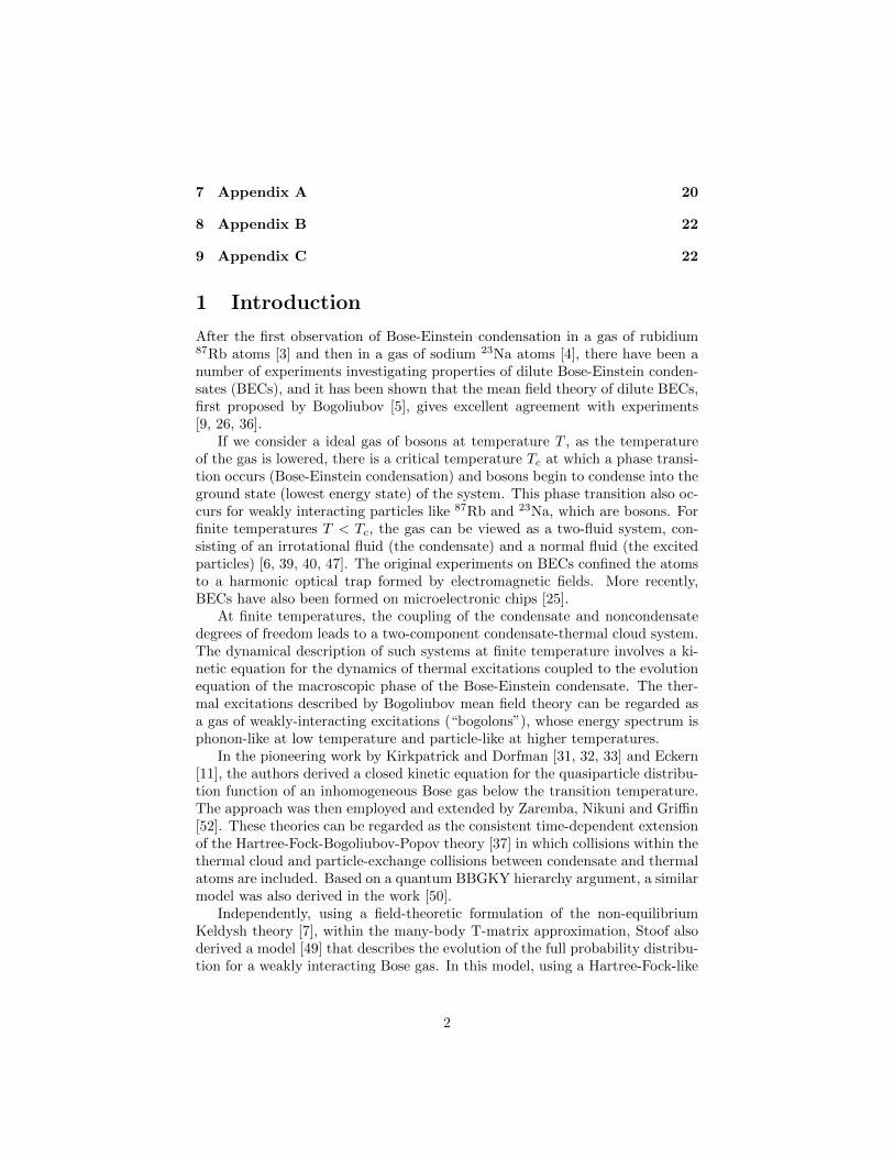
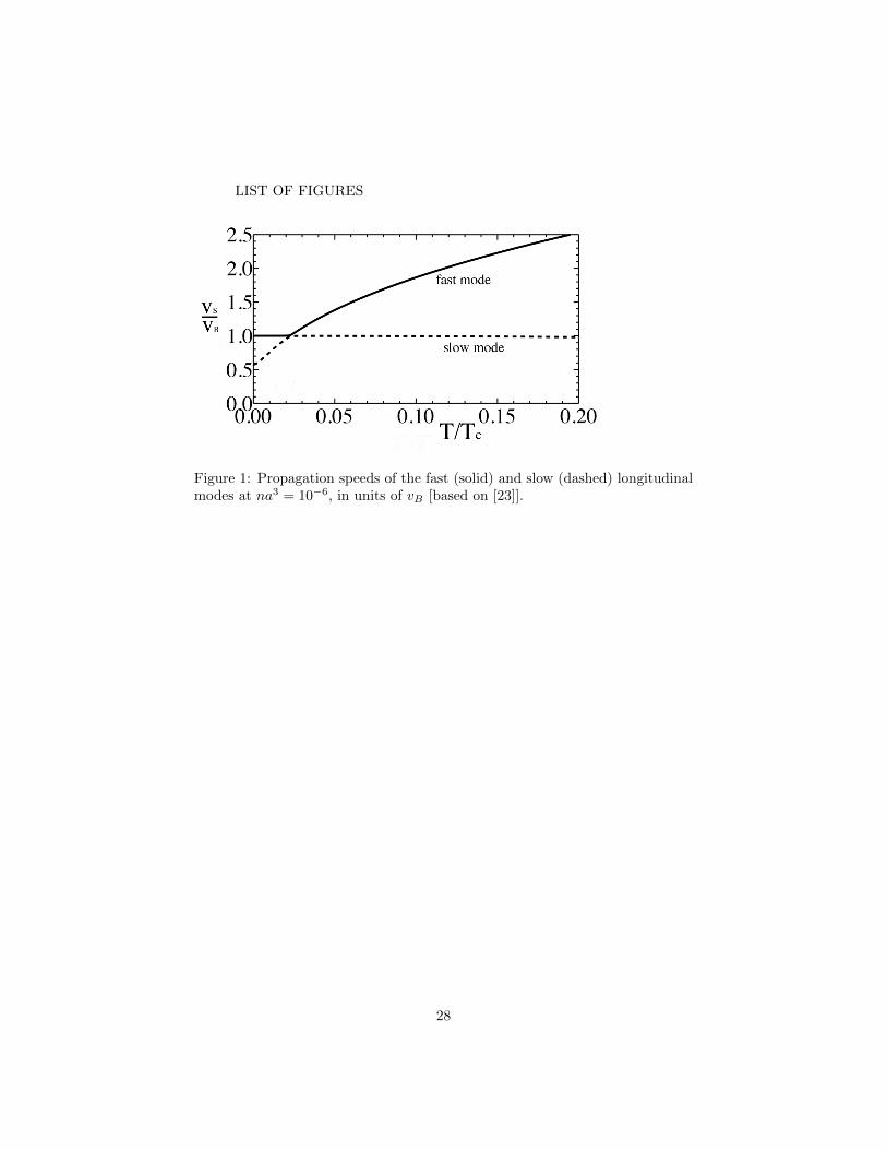
In Fig. 1, we plot the sound speed, in units of the Bogoliubov speed vB , as afunction of fractional distance below the critical temperature for neqa3 = 10−6

[23], which is a value found in experiments. For a rubidium BEC, it would corre-spond to a scattering length a = 5.6×10−9m and a density neq = 5.7×1018m−3.There are several things to note. (i) The speed of both the fast mode and theslow mode approach finite values in the limit T→0 K. This behavior of the soundspeeds is consistent with the behavior of the sound speeds found by Lee andYang [35] using a very different approach. It is a consequence of the fact thatthe bogolon spectrum becomes phonon-like at very low temperature. One doesnot see this behavior of the sound speeds for models with particle-like spectrumat very low temperature [27]. For models with particle-like spectrum, one of thesound speeds goes to zero as T→0 K. (ii) The sound speeds undergo an avoidedcrossing as the temperature is lowered. The temperature at which the avoidedcrossing occurs increases with increasing density of the gas. For neqa3 = 10−5

it occurs at T/Tc≈0.05. For neqa3 = 10−4 it occurs at T/Tc≈0.11 [23].

16

The zeroth order left and right eigenstates can be obtained from the equa-tions Γ†L·M = 0, and M ·ΓR = 0, respectively, once the frequencies are de-termined. For the transverse modes, the left and right eigenstates are com-

plex conjugates of one another and Υ(0)R (k) = Υ

(0)0,1,±1(k). For the longitudinal

modes, the left and right eigenstates are of the form Υ(0)R (k) = Γ0,0,0Υ

(0)0,0,0(k) +

Γ0,1,0Υ(0)0,1,0(k). The exact expression for Γ0,0,0 and Γ0,0,0 for a given mode can

be found by solving M ·ΓR = 0 for the particular first order frequency consid-ered.

4.0.3 Second Order Perturbation Theory

To second order in q, Eq. (4.7) takes the form

ω(2) Υ(0)(k) + ω(1) Υ(1)(k)

− 1

(ω(1))2 − v2B

ghk

m2

√N eq

k

Meqk

1

(2π)3

∫dk1

k1,z

k1

√N eq

k1Meq

k1Υ(1)(k1)

+2ω(1)ω(2)

(ω(1))2 − v2B)2

ghk

m2

√N eq

k

Meqk

1

(2π)3

∫dk1

k1,z

k1

√N eq

k1Meq

k1Υ(0)(k1)

= kzh

m

(εk + Λ0)

EkΥ(1)(k) + i

∫ ∞0

dk1

∫dΩ1 C(k,k1)Υ(2)(k1). (4.16)

The state Υ(1)(k) can be obtained from Eq. (4.10). If we multiply on the

left by Υ(0)L (k) and integrate, we can eliminate the collision operator from this

equation and obtain values for ω(2) for each of the hydrodynamic modes. Thesequantities are the decay rates of the modes.

In order to write explicit expressions for the decay rates, it is useful tointroduce abstract notation. All the eigenfunctions of the collision operatorC(k1,k2) can be written in the form

Υβ,`,m(k) = Υβ,`(k) Ym` (k), (4.17)

where Ym` (k) is a spherical harmonic and k = k/|k|. The eigenstates are or-

thonormalized so that∫ ∞0

dk1

∫dΩ1 Υ∗β1,`1,m1

(k1)Υβ2,`2,m2(k1) = δβ1,β2

δ`1,`2δm1,m2(4.18)

and∫∞

0dk1 Υ∗β1,`

(k1)Υβ2,`(k1) = δβ1,β2. We can also write the collision operator

in a spectral decomposition

C(k1,k2) =

∞∑`=0

∑m=−`

C`(k1, k2) Ym` (k1)Ym∗

` (k2)

=

∞∑β=0

∞∑`=0

∑m=−`

λβ,` Υβ,`,m(k1)Υ∗β,`,m(k2) (4.19)

17

where C`(k1, k2) =∑∞β=0 λβ,` Υβ,`(k1)Υ∗β,`(k2) . Here Υβ,`,m(k1) (with β 6=0)

are eigenstates of C`(k1, k2) with eigenvalues λβ,` < 0.We can now express the operator C`(k1, k2) in “bra-ket” notation as

C` =

∞∑β=0

λβ,`|Υβ,`〉〈Υβ,`|, (4.20)

so that 〈k1|C`|k2〉 = C`(k1, k2) and 〈k|Υβ,`〉 = Υβ,`(k), where 〈k1|k2〉 = δ(k1−k2)and

∫∞0dk |k〉〈k| = 1, where 1 is the unit operator.

The decay rate for the transverse (viscous) modes can be written

ω(2)6 =

1

5

∞∑β=0

1

λβ,2

∣∣〈Υβ,`|kBk|Υβ,2〉∣∣2 (4.21)

where

Bk =h

m

εk + Λ0

Ek(4.22)

The viscosity η of the BEC is related to ω(2)6 via the equation η = ρnω

(2)6 , where

ρn is the density of the normal (non-condensate) part of the the BEC [24].The decay rates for the longitudinal (sound) modes are given by

ω(2) =i

1 + S1

6C0;1 +

1

6C1;0 +

2

15C1;2 + C

′

0

, (4.23)

where

C`′,` =

∞∑β=0

1

λβ,`|〈Υ0,`′ |kBk|Υβ,`〉|2, (4.24)

C′

0 =gh

12π2m2D0,1

1

((ω(1))2 − v2B)

×∞∑β=0

1

λβ,0〈Υ0,`′ |kBk|Υβ,0〉

∫dkkψ∗β,0(k)

√N eq

k

Meqk

(4.25)

and

S =

[(ω(1))2

((ω(1))2 − v2B)2

]gh

m2α

1√3

1

2π2

1

D0,1

∫dkk

√N eq

k

Meqk

ψ0,0(k). (4.26)

The lifetime of the sound modes in the BEC is given by (ω(2)q2)−1 and dependson the speed ω(1) of the sound mode. On the right hand side of (4.23), thefirst three terms are current-current correlation functions similar to those thatdetermine the decay of sound modes in classical gases. The factor of S in thedenominator is a consequence of the macroscopic phase that results from thebroken gauge symmetry in the BEC below T = Tc.

18

4.1 Comparison to Experiment

We can compare the prediction of Eq. (4.23), for the decay rate of sound modesin BECs, to the results found in the Steinhauer experiment [46] in which a soundmode was excited in a 87Rb BEC, and observed to decay. The wavelength ofthe sound wave was about 18×10−6 m (q = 0.35µm−1). The particle densityof the BEC was about neq = 9.71×1019 m−3 which gives a critical temperatureof about Tc = 3.90×10−7 K. The Bogoliubov speed in this case is approx-imately vB ≈ 1.887mm/s, which is approximately the sound speed observedin the experiment [46]. In the experiment, a harmonic trap with frequenciesf1 = f2 = 224 Hz and f3 = 26 Hz was used to create a 1D sound mode. Around〈N〉 = 5×105 atoms in the trap were used, which gives the critical tempera-

ture TC = hm

(〈N〉f1f2f3

1.202

)1/3

≈3.9×10−7. The sound mode had a wave vector

q = 0.35 µm−1 and a lifetime τd∼9 ms. The temperature of the BEC in theexperiment was T = 21±20 nK, which belongs to the temperature regime shownin Figure 2.

The lifetimes τd = i/(ω(2)q2) of the fast and slow sound modes, obtainedfrom Eq. (4.23), are plotted in Figure 2 as a function of temperature for pa-rameters applicable to the Steinhauer experiment. The dotted line corresponds

to the slow modes with speed ±ω(1)2 and the solid line corresponds to the fast

modes with speeds ±ω(1)4 . The life times of the fast and slow sound modes cross

at the same temperature at which the avoided crossing occurs in the fast andslow sound speeds (see Fig. 1). The lifetime of the slow sound mode (dottedline) is of the order of microseconds above the crossing but drops to millisecondsbelow the crossing point. The lifetime of the fast sound mode is of the order ofmilliseconds for temperatures above the crossing point, but then rapidly risesto microseconds for temperatures below the crossing point. The lifetime of thesound mode observed in the experiment was τd∼9 ms. Thus we find, usingthe theory, that the temperature of the experiment was either T = 11±1nK orT = 67±5nK.

It should be noted that we use the uniform density neq = 9.71×1019 m−3,while the density of a BEC in a trap varies slightly in the region that supportsthe sound wave, the change in the decay rates if the density were changedcan be estimated to be 10%. The uncertainty in the prediction, due to a 10%uncertainty in the density is shown in Figure 2 by the faint dashed lines that oneither side of the result for neq = 9.71×1019 m−3. The uncertainty in the densitydoes not significantly change the theoretical prediction for the temperature atwhich sound waves in [46] was measured. Thus, the value of the sound modelifetime, predicted by (2.1) - (2.2) is consistent with that reported in [46].

5 Conclusions

A monatomic BEC has six hydrodynamic modes, two of which are transversemodes and describe viscous properties of the BEC, and the other four modes

19

are longitudinal modes and describe sound mode propagation in the BEC. Amonatomic classical gas has one pair of propagating sound modes, one non-propagating thermal mode, and two non propagating viscous modes. In a BEC,only the viscous modes are non-propagating. A dilute BEC has two pairs ofsound modes, each of which is a mixture of density and temperature waves.

The theory predicts that the two types of sound mode have different speedsand very different lifetimes. Using parameters from the Steinhauer experimenton a rubidium BEC, the theory indicates that one sound mode is long lived(10−2s) and the other short-lived (10−6s). The identity of the long-live modeappears to switch at the temperature of the avoided crossing of the sound speeds.At the temperature of the avoided crossing, neither mode lives a very long time.It has been suggested that this behavior of the sound modes could form thebasis for an accurate way to determine the temperature of the BEC, at very lowtemperature.

6 Acknowledgements

Author LER thanks the Robert A. Welch Foundation (Grant No. F-1051) forsupport of this work. MBT was supported by NSF Grant RNMS (Ki-Net)1107444, ERC Advanced Grant DYCON.

7 Appendix A

We formulate below the form of the collision operator G[η]

G[η](k1) = −N eqk1

(1 +N eqk1)

(M(k1)η(k1)+

+

∫R3

dk2

N eqk2

1 +N eqk1

K(k1,k2)η(k2)) (7.1)

with

M(k1) =

∫R3

dk2

N eqk2

N eqk1

+ 1

2A0TA(k1,k2) +A0

1 +N eqk2

N eqk2

TB(k1,k2)

+B0QA(k1,k2) +B0QB(k1,k2) +1

3

1 +N eqk2

N eqk2

QC(k1,k2)

,

20

K(k1,k2) =

2A0TA(k1,k2)− 2A0

1 +N eqk2

N eqk2

TB(k1,k2)

− 2A0

1 +N eqk1

N eqk1

TB(k2,k1) +B0QA(k1,k2)

− 2B0

1 +N eqk2

N eqk2

RA(k1,k2) + 2B0QB(k1,k2)

−B0

1 +N eqk2

N eqk2

QC(k1,k2)−B0

1 +N eqk1

N eqk1

QC(k2,k1)

.

The functions appearing in the above expressions are defined,

A0 =4πN0g

2

(2π)3hV, B0 =

4πg2

(2π)6h,

TA(k1,k2) =

∫R3

dk3δ(1 + 2− 3)(W 121,2,3)2(N eq

k3+ 1),

TB(k1,k2) =

∫R3

dk3δ(1− 2− 3)(W 123,2,1)2(N eq

k3+ 1),

TB(k2,k1) =

∫R3

dk3δ(2− 1− 3)(W 123,1,2)2(N eq

k3+ 1),

QA(k1,k2) =

∫R3

dk3dk4δ(1 + 2− 3− 4)(W 221,2,3,4)2(N eq

k3+ 1)(N eq

k4+ 1),

RB(k1,k2) =

∫R3

dk3dk4δ(1 + 2− 3− 4)(W 221,3,2,4)2N eq

k3(N eq

k4+ 1),

QB(k1,k2) =

∫R3

dk3dk4δ(1 + 2 + 3− 4)(W 314,3,2,1)2N eq

k3(N eq

k4+ 1),

QC(k1,k2) =

∫R3

dk3dk4δ(1− 2− 3− 4)(W 311,2,3,4)2(N eq

k3+ 1)(N eq

k4+ 1),

(7.2)where

δ(1 + 2− 3− 4)≡δ(k1 + k2 − k3 − k4)δ(E(k1) + E(k2)− E(k3)− E(k4)),

(with similar definitions for δ(1 + 2 − 3) and δ(1 + 2 + 3 − 4). etc), B is thevolume of the box of bosons under consideration, as explained in (3.1),

W 121,2,3 = u1u2u3 − u1v2u3 − v1u2u3 + u1v2v3 + v1u2v3 − v1v2v3, (7.3)

W 221,2,3,4 = u1u2u3u4 + u1v2u3v4 + u1v2v3u4 + v1u2u3v4 + v1u2v3u4 + v1v2v3v4

(7.4)and

W 311,2,3,4 = u1u2u3v4 + u1u2v3u4 + u1v2u3u4 + v1v2v3u4 + v1v2u3v4 + v1u2v3v4.

(7.5)

21

The Bogoliubov factors ui and vi, (i = 1, 2, 3, 4), are given by

ui = uk1 =1√2

√1 +

εki+ Λ0

Eki

and

vi = vki =1√2

√εki

+ Λ0

Eki

− 1.

8 Appendix B

When the BEC is in equilibrium, the mean field Hamiltonian (in the superfluidrest frame) takes the form [44]

H0 =∑i

[(εi − Λ0)a†i ai +

Λ0

2

(a†i ai + a†i ai

)]=g

2N2

0 +∑i

Eib†i bi, (8.1)

where

E1 =

√e2

1 − Λ02 with e1 =

h2k21

2m+ ν0 − µ =

h2k21

2m+ Λ0 (8.2)

and we have used the Hugenholtz-Pines relation µ = ν0 − Λ0 [19]. In termsof these equilibrium quantities, the Bogoliubov transformation parameters takethe form

u1 =1√2

√1 +

e1

E1, v1 =

1√2

√e1

E1− 1 (8.3)

Note also that

u21− v2

1 = 1, Λ0(u21 + v2

1)− 2e1u1v1 = 0, e1(u21 + v2

1)− 2Λ0u1v1 = E1. (8.4)

This transformation has the property that

U−11 ·

(e1 Λ0

−Λ0 −e1

)·U1 = U1·

(e1 −Λ0

Λ0 −e1

)·U−1

1 =

(E1 00 −E1

). (8.5)

9 Appendix C

The collision operator operator C(k,k1), that appears in Eq. (4.5), can beexpanded in spherical harmonics which determine on the angular directions ofthe momenta k and k1.

C(k,k1) =

∞∑`=0

∑m=−`

C`(k, k1)Ym` (k)Ym∗

` (k1) (9.1)

The collision operator C(k,k1) is a symmetric operator and has a complete setof orthonormal eigenfunctions.

22

The eigenvalues λβ,` and eigenstates Υβ,`,m(k1) of the operator C(k1,k2),satisfy the conditions∫

dk2 C(k1,k2)Υ(0)β,`,m(k2) = λβ,`Υ

(0)β,`,m(k1). (9.2)

and ∫dk1 Υ

(0)β,`,m(k1) C(k1,k2) = λβ,`Υ

(0)β,`,m(k2). (9.3)

The eigenvalues λβ,` are independent of m due to the angular symmetry of thecollision operator.

The bogolon momentum and energy are conserved during collisions, althoughbogolon number is not. Therefore, Gk1

h, acting on four conserved quantities,h = Ek, h = kx, h = ky, and h = kz, gives zero. We can use this fact to formfour eigenstates of C(k1,k2). We write them in the form

Υ(0)0,0,0(k1) = Υ0,0(k1)Y0

0(k1), Υ(0)

0,1,0(k1) = Υ0,1(k1)Y0

1(k1),

Υ(0)0,1,1(k1) = Υ0,1(k1)Y1

1(k1), Υ(0)0,1,−1(k1) = Υ0,1(k1)Y−1

1 (k1). (9.4)

where Υ0,0(k) = D0,0Ek√k2N eq

k Feqk and Υ0,1(k) = D0,1k

√k2N eq

k Feqk . The

quantities Dβ,`, are normalization constants given by

D0,0 =

(∫ ∞0

dkk2E2kN

eqk F

eqk

)−1/2

and D0,1 =

(∫ ∞0

dkk4N eqk F

eqk

)−1/2

.(9.5)

The corresponding eigenvalues λβ,` are independent of m and degenerate sothat λ0,0 = λ0,1 = 0 and λ0,1 is three-fold degenerate. The eigenstates can beorthonormalized so that∫ ∞

0

dk1

∫dΩ1 Υ

(0)∗β1,`1,m1

(k1)Υ(0)β2,`2,m2

(k1) = δβ1,β2δ`1,`2δm1,m2 (9.6)

and∫∞

0dk1 Υ∗β1,`

(k1)Υβ2,`(k1) = δβ1,β2 . We can now write the spectral decom-position of the collision operator

C(k1,k2) =

∞∑β=0

∞∑`=0

∑m=−`

λβ,` Υ(0)β,`,m(k1)Υ

(0)∗β,`,m(k2)

(9.7)

where C`(k1, k2) =∑∞β=0 λβ,` Υβ,`(k1)Υ∗β,`(k2) . These four eigenfunctions

form the basis for the hydrodynamic modes in the BEC. They correspond toquantities that are conserved on the microscopic scale.

23

References

[1] A. I. Akhiezer and S. V. Peletminskiı. Methods of statistical physics, vol-ume 104 of International Series in Natural Philosophy. Pergamon Press,Oxford-Elmsford, N.Y., 1981. With a foreword by N. N. Bogoliubov [N. N.Bogolyubov], Translated from the Russian by M. Schukin.

[2] A. J. Allen, C. F. Barenghi, N. P. Proukakis, and E. Zaremba. A dynamicalself-consistent finite temperature kinetic theory: The zng scheme. arXivpreprint arXiv:1206.0145, 2012.

[3] M.H. Anderson, J.R. Ensher, M.R. Matthews, C.E. Wieman, and E.A. Cor-nell. Observation of BoseEinstein Condensation in a dilute atomic vapor.Science, 269(5221):198–201, 1995.

[4] M. R. Andrews, C. G. Townsend, H.-J. Miesner, D. S. Durfee, D. M. Kurn,and W. Ketterle. Observation of interference between two Bose conden-sates. Science, 275 (5300):637–641, 1997.

[5] N. N. Bogoliubov. Studies in Statistical Mechanics, volume 3 of Edited by J.de Boer and G. R. Uhlenbeck. North-Holland, Amsterdam, North-Holland,Amsterdam, 1962.

[6] F. Dalfovo, S. Giorgini, L. P. Pitaevskii, and S. Stringari. Theory ofbose-einstein condensation in trapped gases. Reviews of Modern Physics,71(3):463, 1999.

[7] P. Danielewicz. Quantum theory of nonequilibrium processes, i. Annals ofPhysics, 152(2):239–304, 1984.

[8] M. J. Davis, C. W. Gardiner, and R. J. Ballagh. Quantum kinetic theory.vii. the influence of vapor dynamics on condensate growth. Physical ReviewA, 62(6):063608, 2000.

[9] R. J. Dodd, M. Edwards, C. W. Clark, and K. Burnett. Collective exci-tations of bose-einstein-condensed gases at finite temperatures. PhysicalReview A, 57(1):R32, 1998.

[10] R. A. Duine and H. T. C. Stoof. Stochastic dynamics of a trapped bose-einstein condensate. Physical Review A, 65(1):013603, 2001.

[11] U. Eckern. Relaxation processes in a condensed bose gas. J. Low Temp.Phys., 54:333–359, 1984.

[12] C. Gardiner and P. Zoller. Quantum kinetic theory. A quantum kineticmaster equation for condensation of a weakly interacting Bose gas withouta trapping potential. Phys. Rev. A, 55:2902, 1997.

[13] C. Gardiner and P. Zoller. Quantum kinetic theory. III. Quantum kineticmaster equation for strongly condensed trapped systems. Phys. Rev. A,58:536, 1998.

24

[14] C. Gardiner and P. Zoller. Quantum kinetic theory. V. Quantum kineticmaster equation for mutual interaction of condensate and noncondensate.Phys. Rev. A, 61:033601, 2000.

[15] C. Gardiner and P. Zoller. Quantum noise: a handbook of Markovian andnon-Markovian quantum stochastic methods with applications to quantumoptics, volume 56. Springer Science & Business Media, 2004.

[16] C. W. Gardiner, M. D. Lee, R. J. Ballagh, M. J. Davis, and P. Zoller.Quantum kinetic theory of condensate growth: Comparison of experimentand theory. Physical review letters, 81(24):5266, 1998.

[17] C. W. Gardiner, M. D. Lee, R. J. Ballagh, M. J. Davis, and P. Zoller. Roleof quasiparticles in the growth of a trapped bose-einstein condensate. arXivpreprint cond-mat/9801027, 1998.

[18] C. W. Gardiner, P. Zoller, R. J. Ballagh, and M. J. Davis. Kinetics ofbose-einstein condensation in a trap. Physical review letters, 79(10):1793,1997.

[19] N. M. Hugenholtz and D. Pines. Ground-state energy and excitation spec-trum of a system of interacting bosons. Physical Review, 116(3):489, 1959.

[20] E. D Gust and L. E. Reichl. Collision integrals in the kinetic equationsofdilute bose-einstein condensates. arXiv:1202.3418, 2012.

[21] E. D. Gust and L. E. Reichl. Relaxation modes in bose–einstein conden-sates. Physica Scripta, 2012(T151):014057, 2012.

[22] E. D Gust and L. E. Reichl. Relaxation rates and collision integrals forbose-einstein condensates. Phys. Rev. A, 170:43–59, 2013.

[23] E. D. Gust and L. E. Reichl. Decay of hydrodynamic modes in diluteBose-Einstein condensates. Physical Review A, 90:043615, 2014.

[24] E. D. Gust and L. E. Reichl. The viscosity of dilute bose–einstein conden-sates. Physica Scripta, 2015(T165):014034, 2015.

[25] W. Hansel, P. Hommelhoff, T. W. Hansch, and J. Reichel. Bose-einsteincondensation on a microelectronic chip. Nature, 413(6855):498, 2001.

[26] D. A. W. Hutchinson, E. Zaremba, and A. Griffin. Finite temperatureexcitations of a trapped bose gas. Physical review letters, 78(10):1842,1997.

[27] A. Griffin and E. Zaremba. First and second sound in a uniform bose gas.Physical Review A, 56(6):4839, 1997.

[28] M. Imamovic-Tomasovic and A. Griffin. Quasiparticle kinetic equation ina trapped bose gas at low temperatures. J. Low Temp. Phys., 122:617–655,2001.

25

[29] D. Jaksch, C. Gardiner, K. M. Gheri, and P. Zoller. Quantum kinetic the-ory. IV. Intensity and amplitude fluctuations of a Bose-Einstein condensateat finite temperature including trap loss. Phys. Rev. A, 58:1450, 1998.

[30] D. Jaksch, C. Gardiner, and P. Zoller. Quantum kinetic theory. II. Simu-lation of the quantum Boltzmann master equation. Phys. Rev. A, 56:575,1997.

[31] T. R. Kirkpatrick and J. R. Dorfman. Transport theory for a weakly inter-acting condensed Bose gas. Phys. Rev. A (3), 28(4):2576–2579, 1983.

[32] T. R. Kirkpatrick and J. R. Dorfman. Transport coefficients in a dilute butcondensed bose gas. J. Low Temp. Phys., 58:399–415, 1985.

[33] T. R. Kirkpatrick and J. R. Dorfman. Transport in a dilute but condensednonideal bose gas: Kinetic equations. J. Low Temp. Phys., 58:301–331,1985.

[34] M. D. Lee and C. W. Gardiner. Quantum kinetic theory. vi. the growth ofa bose-einstein condensate. Physical Review A, 62(3):033606, 2000.

[35] T.-D. Lee and C.-N. Yang. Question of parity conservation in weak inter-actions. Physical Review, 104(1):254, 1956.

[36] S. A. Morgan. A gapless theory of bose-einstein condensation in dilutegases at finite temperature. Journal of Physics B: Atomic, Molecular andOptical Physics, 33(19):3847, 2000.

[37] T. Nikuni, E. Zaremba and A. Griffin Bose-condensed gases at finitetemperatures. Cambridge University Press, Cambridge, 2009.

[38] S. Peletminskii and A. Yatsenko. Contribution to the quantum theory ofkinetic and relaxation process. Soviet Physics JETP, 26(773), 1968.

[39] C. J. Pethick and H. Smith. Bose-Einstein condensation in dilute gases.Cambridge university press, 2002.

[40] L. Pitaevskii and S. Stringari. Bose-Einstein condensation and superfluid-ity, volume 164. Oxford University Press, 2016.

[41] N. Proukakis, S. Gardiner, M. Davis, and M. Szymanska. Quantum Gases:Finite temperature and non-equilibrium dynamics, volume 1. World Scien-tific, 2013.

[42] L. E. Reichl. Microscopic modes in a Fermi superfluid. I. Linearized kineticequations. J. Statist. Phys., 23(1):83–110, 1980.

[43] L. E. Reichl. Microscopic modes in a Fermi superfluid. II. Dispersion rela-tions. J. Statist. Phys., 23(1):111–125, 1980.

26

[44] L. E. Reichl and E. D Gust. Transport theory for a dilute bose-einsteincondensate. J Low Temp Phys, 88:053603, 2013.

[45] R. Schley, A. Berkovitz, S. Rinott, I. Shammass, A. Blumkin, and J. Stein-hauer. Planck distribution of phonons in a bose-einstein condensate. Phys-ical review letters, 111(5):055301, 2013.

[46] I. Shammass, S. Rinott, A. Berkovitz, R. Schley, and J. Steinhauer. Phonondispersion relation of an atomic bose-einstein condensate. Physical reviewletters, 109(19):195301, 2012.

[47] H. Spohn. Kinetics of the bose-einstein condensation. Physica D, 239:627–634, 2010.

[48] H. T. C. Stoof. Initial stages of bose-einstein condensation. Physical reviewletters, 78(5):768, 1997.

[49] H. T. C. Stoof. Coherent versus incoherent dynamics during bose-einsteincondensation in atomic gases. J. Low Temp. Phys., 114:11–108, 1999.

[50] S. M’etens Y. Pomeau, M.A. Brachet and S. Rica. Theorie cinetique d’ungaz de bose dilue avec condensat. C. R. Acad. Sci. Paris S’er. IIb M’ec.Phys. Astr., 327:791–798, 1999.

[51] E. Wigner. On the quantum correction for thermodynamic equilibrium.Physical review, 40(5):749, 1932.

[52] E. Zaremba, T. Nikuni, and A. Griffin. Dynamics of trapped bose gases atfinite temperatures. J. Low Temp. Phys., 116:277–345, 1999.

27

LIST OF FIGURES

Figure 1: Propagation speeds of the fast (solid) and slow (dashed) longitudinalmodes at na3 = 10−6, in units of vB [based on [23]].

28

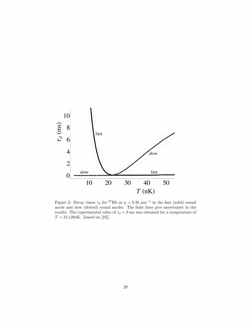
Figure 2: Decay times τd for 87Rb at q = 0.35 µm−1 in the fast (solid) soundmode and slow (dotted) sound modes. The faint lines give uncertainty in theresults. The experimental value of τd = 9 ms was obtained for a temperature ofT = 21±20nK. [based on [23]].

29