A Kalman‐filter bias correction method applied to deterministic, ensemble averaged and probabilistic forecasts of surface ozone

Tellus (2008), 60B, 238–249 Journal compilation C© 2008 Blackwell MunksgaardNo claim to original US government works

Printed in Singapore. All rights reservedT E L L U S

A Kalman-filter bias correction method applied todeterministic, ensemble averaged and probabilistic

forecasts of surface ozone

By LUCA DELLE MONACHE 1,2∗, JAMES WILCZAK 3, STUART MCKEEN 4,5,

GEORG GRELL 4,6, MARIUSZ PAGOWSKI 6,7, STEVEN PECKHAM 4,6, ROLAND STULL 1,

JOHN MCHENRY 8 and JEFFREY MCQUEEN 9, 1Atmospheric Science Programme, Earth and OceanSciences Department, University of British Columbia, Vancouver, British Columbia, Canada; 2Now at Lawrence

Livermore National Laboratory, Livermore, CA, USA; 3Physical Sciences Division, Earth System ResearchLaboratory, National Oceanic and Atmospheric Administration, Boulder, CO, USA; 4Cooperative Institute for

Research in Environmental Sciences, University of Colorado, Boulder, CO, USA; 5Chemical Sciences Division, EarthSystem Research Laboratory, National Oceanic and Atmospheric Administration, Boulder, CO, USA; 6Global SystemsDivision, Earth System Research Laboratory, National Oceanic and Atmospheric Administration, Boulder, CO, USA;

7Cooperative Institute for Research in the Atmosphere, Colorado State University, Fort Collins, CO, USA; 8BaronAdvanced Meteorological Systems, c/o North Carolina State University, Raleigh, NC, USA; 9National Weather Service/ National Centers for Environmental Prediction/National Oceanic and Atmospheric Administration, Camp Springs,

MD, USA

(Manuscript received 26 June 2007; in final form 12 November 2007)

ABSTRACT

Kalman filtering (KF) is used to estimate systematic errors in surface ozone forecasts. The KF updates its estimate of

future ozone-concentration bias using past forecasts and observations. The optimum filter parameter is estimated via

sensitivity analysis. KF performance is tested for deterministic, ensemble-averaged and probabilistic forecasts. Eight

simulations were run for 56 d during summer 2004 over northeastern USA and southern Canada, with 358 ozone surface

stations.

KF improves forecasts of ozone-concentration magnitude (measured by root mean square error) and the ability

to predict rare events (measured by the critical success index), for deterministic and ensemble-averaged forecasts. It

improves the 24-h maximum ozone-concentration prediction (measured by the unpaired peak prediction accuracy),

and improves the linear dependency and timing of forecasted and observed ozone concentration peaks (measured by

a lead/lag correlation). KF also improves the predictive skill of probabilistic forecasts of concentration greater than

thresholds of 10–50 ppbv, but degrades it for thresholds of 70–90 ppbv. KF reduces probabilistic forecast bias. The

combination of KF and ensemble averaging presents a significant improvement for real-time ozone forecasting because

KF reduces systematic errors while ensemble-averaging reduces random errors. When combined, they produce the best

overall ozone forecast.

1. Introduction

The skill of deterministic ozone forecasts can be improved us-

ing ensemble methods (e.g. Delle Monache and Stull, 2003;

McKeen et al., 2005; Delle Monache et al., 2006a, Mallet and

Sportisse, 2006; Wilczak et al., 2006; Thunis et al., 2007; van

Loon et al., 2007), by combining weighted ensemble averaging

∗Corresponding author.

e-mail: [email protected]

DOI: 10.1111/j.1600-0889.2007.00332.x

with the application of linear regression (Pagowski et al., 2005)

or dynamic linear regression (Pagowski et al., 2006), and with

bias removal methods (e.g. McKeen et al., 2005; Wilczak et al.,

2006; Delle Monache et al., 2006b, hereinafter referred to as

DM06b).

Forecast bias (i.e. systematic error) is a problem common to all

chemistry transport models (CTMs) (Russell and Dennis, 2000).

This study evaluates the ability of the Kalman filter (KF) pre-

dictor post-processing bias-removal method in predicting biases

of surface ozone forecasts. The KF correction is an automatic

post-processing method that uses past observations and forecasts

238 Tellus 60B (2008), 2

KF BIAS CORRECTION METHOD APPLIED TO DETERMINISTIC 239

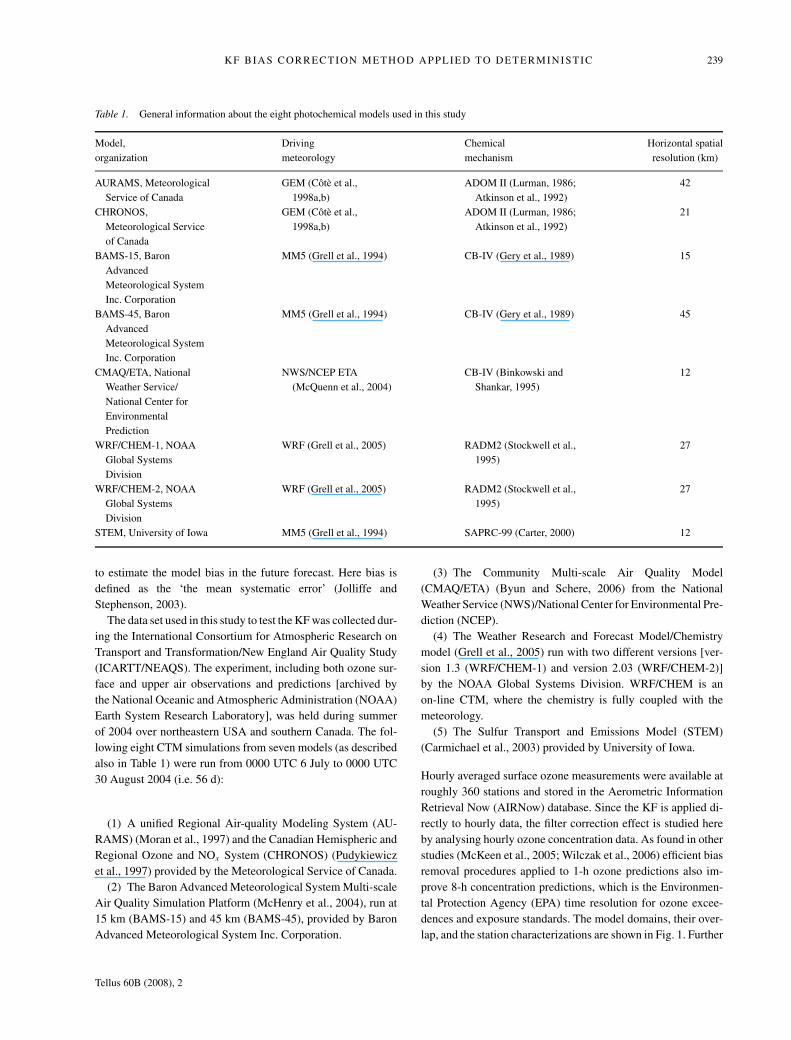
Table 1. General information about the eight photochemical models used in this study

Model, Driving Chemical Horizontal spatial

organization meteorology mechanism resolution (km)

AURAMS, Meteorological

Service of Canada

GEM (Cote et al.,

1998a,b)

ADOM II (Lurman, 1986;

Atkinson et al., 1992)

42

CHRONOS,

Meteorological Service

of Canada

GEM (Cote et al.,

1998a,b)

ADOM II (Lurman, 1986;

Atkinson et al., 1992)

21

BAMS-15, Baron

Advanced

Meteorological System

Inc. Corporation

MM5 (Grell et al., 1994) CB-IV (Gery et al., 1989) 15

BAMS-45, Baron

Advanced

Meteorological System

Inc. Corporation

MM5 (Grell et al., 1994) CB-IV (Gery et al., 1989) 45

CMAQ/ETA, National

Weather Service/

National Center for

Environmental

Prediction

NWS/NCEP ETA

(McQuenn et al., 2004)

CB-IV (Binkowski and

Shankar, 1995)

12

WRF/CHEM-1, NOAA

Global Systems

Division

WRF (Grell et al., 2005) RADM2 (Stockwell et al.,

1995)

27

WRF/CHEM-2, NOAA

Global Systems

Division

WRF (Grell et al., 2005) RADM2 (Stockwell et al.,

1995)

27

STEM, University of Iowa MM5 (Grell et al., 1994) SAPRC-99 (Carter, 2000) 12

to estimate the model bias in the future forecast. Here bias is

defined as the ‘the mean systematic error’ (Jolliffe and

Stephenson, 2003).

The data set used in this study to test the KF was collected dur-

ing the International Consortium for Atmospheric Research on

Transport and Transformation/New England Air Quality Study

(ICARTT/NEAQS). The experiment, including both ozone sur-

face and upper air observations and predictions [archived by

the National Oceanic and Atmospheric Administration (NOAA)

Earth System Research Laboratory], was held during summer

of 2004 over northeastern USA and southern Canada. The fol-

lowing eight CTM simulations from seven models (as described

also in Table 1) were run from 0000 UTC 6 July to 0000 UTC

30 August 2004 (i.e. 56 d):

(1) A unified Regional Air-quality Modeling System (AU-

RAMS) (Moran et al., 1997) and the Canadian Hemispheric and

Regional Ozone and NOx System (CHRONOS) (Pudykiewicz

et al., 1997) provided by the Meteorological Service of Canada.

(2) The Baron Advanced Meteorological System Multi-scale

Air Quality Simulation Platform (McHenry et al., 2004), run at

15 km (BAMS-15) and 45 km (BAMS-45), provided by Baron

Advanced Meteorological System Inc. Corporation.

(3) The Community Multi-scale Air Quality Model

(CMAQ/ETA) (Byun and Schere, 2006) from the National

Weather Service (NWS)/National Center for Environmental Pre-

diction (NCEP).

(4) The Weather Research and Forecast Model/Chemistry

model (Grell et al., 2005) run with two different versions [ver-

sion 1.3 (WRF/CHEM-1) and version 2.03 (WRF/CHEM-2)]

by the NOAA Global Systems Division. WRF/CHEM is an

on-line CTM, where the chemistry is fully coupled with the

meteorology.

(5) The Sulfur Transport and Emissions Model (STEM)

(Carmichael et al., 2003) provided by University of Iowa.

Hourly averaged surface ozone measurements were available at

roughly 360 stations and stored in the Aerometric Information

Retrieval Now (AIRNow) database. Since the KF is applied di-

rectly to hourly data, the filter correction effect is studied here

by analysing hourly ozone concentration data. As found in other

studies (McKeen et al., 2005; Wilczak et al., 2006) efficient bias

removal procedures applied to 1-h ozone predictions also im-

prove 8-h concentration predictions, which is the Environmen-

tal Protection Agency (EPA) time resolution for ozone excee-

dences and exposure standards. The model domains, their over-

lap, and the station characterizations are shown in Fig. 1. Further

Tellus 60B (2008), 2

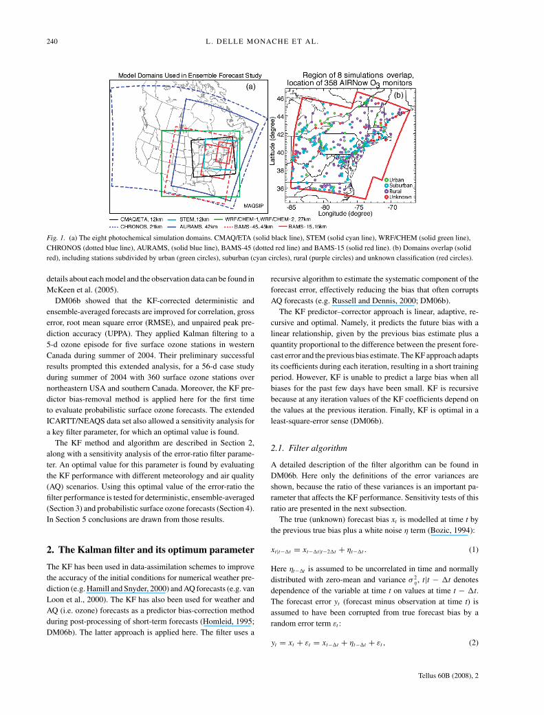
240 L. DELLE MONACHE ET AL.

Fig. 1. (a) The eight photochemical simulation domains. CMAQ/ETA (solid black line), STEM (solid cyan line), WRF/CHEM (solid green line),

CHRONOS (dotted blue line), AURAMS, (solid blue line), BAMS-45 (dotted red line) and BAMS-15 (solid red line). (b) Domains overlap (solid

red), including stations subdivided by urban (green circles), suburban (cyan circles), rural (purple circles) and unknown classification (red circles).

details about each model and the observation data can be found in

McKeen et al. (2005).

DM06b showed that the KF-corrected deterministic and

ensemble-averaged forecasts are improved for correlation, gross

error, root mean square error (RMSE), and unpaired peak pre-

diction accuracy (UPPA). They applied Kalman filtering to a

5-d ozone episode for five surface ozone stations in western

Canada during summer of 2004. Their preliminary successful

results prompted this extended analysis, for a 56-d case study

during summer of 2004 with 360 surface ozone stations over

northeastern USA and southern Canada. Moreover, the KF pre-

dictor bias-removal method is applied here for the first time

to evaluate probabilistic surface ozone forecasts. The extended

ICARTT/NEAQS data set also allowed a sensitivity analysis for

a key filter parameter, for which an optimal value is found.

The KF method and algorithm are described in Section 2,

along with a sensitivity analysis of the error-ratio filter parame-

ter. An optimal value for this parameter is found by evaluating

the KF performance with different meteorology and air quality

(AQ) scenarios. Using this optimal value of the error-ratio the

filter performance is tested for deterministic, ensemble-averaged

(Section 3) and probabilistic surface ozone forecasts (Section 4).

In Section 5 conclusions are drawn from those results.

2. The Kalman filter and its optimum parameter

The KF has been used in data-assimilation schemes to improve

the accuracy of the initial conditions for numerical weather pre-

diction (e.g. Hamill and Snyder, 2000) and AQ forecasts (e.g. van

Loon et al., 2000). The KF has also been used for weather and

AQ (i.e. ozone) forecasts as a predictor bias-correction method

during post-processing of short-term forecasts (Homleid, 1995;

DM06b). The latter approach is applied here. The filter uses a

recursive algorithm to estimate the systematic component of the

forecast error, effectively reducing the bias that often corrupts

AQ forecasts (e.g. Russell and Dennis, 2000; DM06b).

The KF predictor–corrector approach is linear, adaptive, re-

cursive and optimal. Namely, it predicts the future bias with a

linear relationship, given by the previous bias estimate plus a

quantity proportional to the difference between the present fore-

cast error and the previous bias estimate. The KF approach adapts

its coefficients during each iteration, resulting in a short training

period. However, KF is unable to predict a large bias when all

biases for the past few days have been small. KF is recursive

because at any iteration values of the KF coefficients depend on

the values at the previous iteration. Finally, KF is optimal in a

least-square-error sense (DM06b).

2.1. Filter algorithm

A detailed description of the filter algorithm can be found in

DM06b. Here only the definitions of the error variances are

shown, because the ratio of these variances is an important pa-

rameter that affects the KF performance. Sensitivity tests of this

ratio are presented in the next subsection.

The true (unknown) forecast bias xt is modelled at time t by

the previous true bias plus a white noise η term (Bozic, 1994):

xt |t−�t = xt−�t |t−2�t + ηt−�t . (1)

Here ηt−�t is assumed to be uncorrelated in time and normally

distributed with zero-mean and variance σ 2η, t|t − �t denotes

dependence of the variable at time t on values at time t − �t.The forecast error yt (forecast minus observation at time t) is

assumed to have been corrupted from true forecast bias by a

random error term εt :

yt = xt + εt = xt−�t + ηt−�t + εt , (2)

Tellus 60B (2008), 2

KF BIAS CORRECTION METHOD APPLIED TO DETERMINISTIC 241

where again εt is assumed uncorrelated in time and normally

distributed with zero-mean and variance σ 2ε . Thus, yt includes

systematic and random errors.

2.2. Error-ratio parameter sensitivity tests

The KF performance is sensitive to the error ratio σ 2η/σ

2ε . If the

ratio is too high, the forecast-error white-noise variance (σ 2ε) will

be relatively small compared to the true forecast-bias white-noise

variance (σ 2η). Therefore, the filter will put excessive confidence

on the previous forecast, and the predicted bias will respond very

quickly to previous forecast errors. On the other hand, if the ratio

is too low, the predicted bias will change too slowly over time.

Consequently, there exists an optimal value for the ratio that is

given by the climatology of the forecast region, which can be

estimated by evaluating the filter performance in different sit-

uations with different meteorology and different AQ scenarios

(not only for a single AQ episode as in DM06b). In this study,

an optimal value is found that improves real-time surface ozone

forecasts for the largest number of ozone cases, with the largest

number of simulations. Nevertheless, it is recognized that pre-

dictions over different areas (e.g. rural versus urban), or different

model forecasts may have different optimal ratio values.

As described in Section 1, the ICARTT/NEAQS data set offers

a unique opportunity to thoroughly test the filter performance,

both because of its duration (56 d of summer 2004), and due to

the inclusion of eight different photochemical simulations. The

raw and KF-corrected predictions from these simulations can be

tested against surface observations from roughly 360 stations (for

hourly ozone concentrations over the Northeast United States

and Southeast Canada; McKeen et al., 2005). Specifically, with

the ICARTT/NEAQS data set, an optimal error-ratio value can

be estimated to produce a more accurate correction of ozone

forecasts with the KF post-processing predictor method.

DM06b used a ratio value (0.01) from previous studies where

the KF was used to bias-correct weather forecasts, close to

the optimal value (0.06) found by Homleid (1995), who tested

the filter for weather forecasts as well. Here the optimal ratio

value (for ozone surface forecasts) is found by looking at the

average value of the following statistical parameters over the

available surface ozone stations:

1. Pearson product-moment coefficient of linear correlation

(herein ‘correlation’):

correlation =∑Npoint

i=1

{[Co(i) − Co][Cp(i) − Cp]

}√∑Npoint

i=1

[Co(i) − Co

]2 ∑Npoint

i=1

[Cp(i) − Cp

]2(3)

2. RMSE:

RMSE =√

1

Npoint

∑Npoint

i=1[Cp(i) − Co(i)]2. (4)

Here Npoint is the number of all valid observation/prediction cou-

ples of 1-h average concentrations over the 56-d period and 358

stations, Co(i) is the 1-h average observed concentration at a

monitoring station for hour t, Cp(i) is the 1-h average predicted

concentration at a monitoring station for hour t, Co is the av-

erage of 1-h average observed concentrations over all the Npoint

observation/prediction couples available, and Cp is the average

of 1-h average predicted concentrations over all the Npoint obser-

vation/prediction couples available.

Correlation determines the extent to which the observed and

predicted ozone concentration values are linearly related. RMSE

gives important information about the skill of a forecast in pre-

dicting the magnitude of ozone concentration. It is also very

helpful for understanding the filter performance, because it can

be decomposed into systematic and unsystematic components

(Section 3.2).

Since KF is optimal in a least-square-error sense (i.e. is de-

signed to reduce RMSE) the filter optimum is chosen by evaluat-

ing its sensitivity with the RMSE metric. Correlation is included

in this sensitivity analysis to assure the validity of the chosen

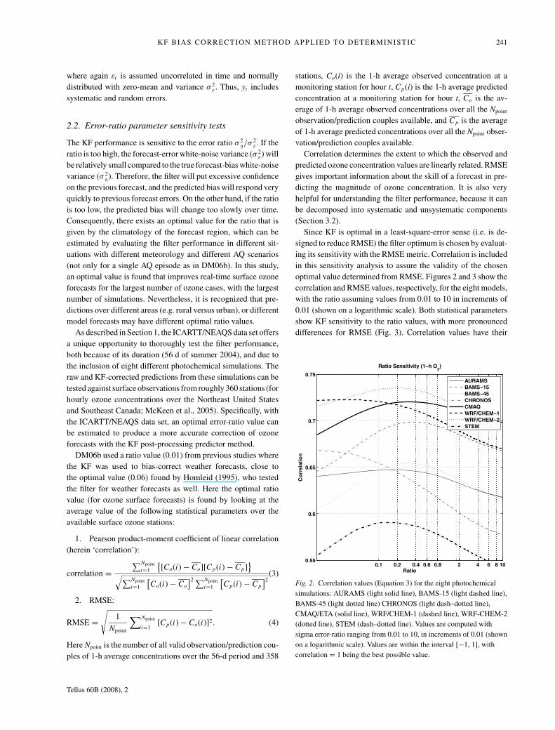
optimal value determined from RMSE. Figures 2 and 3 show the

correlation and RMSE values, respectively, for the eight models,

with the ratio assuming values from 0.01 to 10 in increments of

0.01 (shown on a logarithmic scale). Both statistical parameters

show KF sensitivity to the ratio values, with more pronounced

differences for RMSE (Fig. 3). Correlation values have their

0.1 0.2 0.4 0.6 0.8 2 4 6 8 100.55

0.6

0.65

0.7

0.75

Ratio

Co

rre

lati

on

O3)

AURAMS

BAMS 15

BAMS 45

CHRONOS

CMAQ

WRF/CHEM 1

WRF/CHEM 2

STEM

Fig. 2. Correlation values (Equation 3) for the eight photochemical

simulations: AURAMS (light solid line), BAMS-15 (light dashed line),

BAMS-45 (light dotted line) CHRONOS (light dash–dotted line),

CMAQ/ETA (solid line), WRF/CHEM-1 (dashed line), WRF-CHEM-2

(dotted line), STEM (dash–dotted line). Values are computed with

sigma error-ratio ranging from 0.01 to 10, in increments of 0.01 (shown

on a logarithmic scale). Values are within the interval [−1, 1], with

correlation = 1 being the best possible value.

Tellus 60B (2008), 2

242 L. DELLE MONACHE ET AL.

0.1 0.2 0.4 0.6 0.8 2 4 6 8 1010

15

20

25

30

35

Ratio

RM

SE

(p

pb

v)

O3)

AURAMS

BAMS 15

BAMS 45

CHRONOS

CMAQ/ETA

WRF/CHEM 1

WRF/CHEM 2

STEM

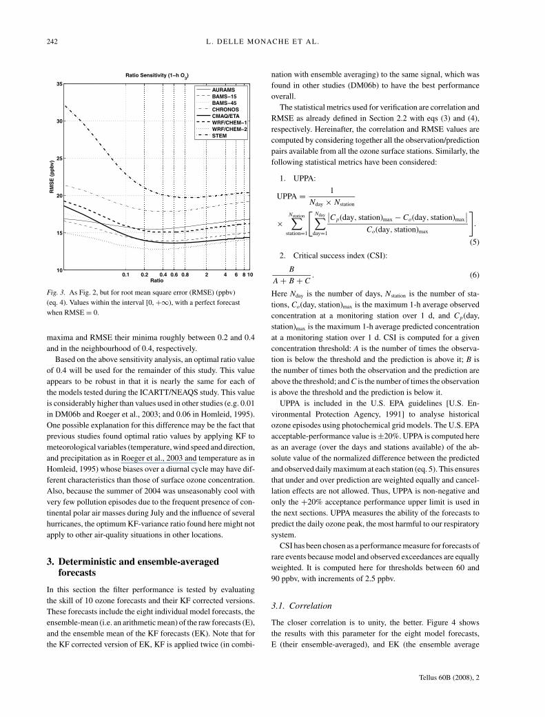
Fig. 3. As Fig. 2, but for root mean square error (RMSE) (ppbv)

(eq. 4). Values within the interval [0, +∞), with a perfect forecast

when RMSE = 0.

maxima and RMSE their minima roughly between 0.2 and 0.4

and in the neighbourhood of 0.4, respectively.

Based on the above sensitivity analysis, an optimal ratio value

of 0.4 will be used for the remainder of this study. This value

appears to be robust in that it is nearly the same for each of

the models tested during the ICARTT/NEAQS study. This value

is considerably higher than values used in other studies (e.g. 0.01

in DM06b and Roeger et al., 2003; and 0.06 in Homleid, 1995).

One possible explanation for this difference may be the fact that

previous studies found optimal ratio values by applying KF to

meteorological variables (temperature, wind speed and direction,

and precipitation as in Roeger et al., 2003 and temperature as in

Homleid, 1995) whose biases over a diurnal cycle may have dif-

ferent characteristics than those of surface ozone concentration.

Also, because the summer of 2004 was unseasonably cool with

very few pollution episodes due to the frequent presence of con-

tinental polar air masses during July and the influence of several

hurricanes, the optimum KF-variance ratio found here might not

apply to other air-quality situations in other locations.

3. Deterministic and ensemble-averagedforecasts

In this section the filter performance is tested by evaluating

the skill of 10 ozone forecasts and their KF corrected versions.

These forecasts include the eight individual model forecasts, the

ensemble-mean (i.e. an arithmetic mean) of the raw forecasts (E),

and the ensemble mean of the KF forecasts (EK). Note that for

the KF corrected version of EK, KF is applied twice (in combi-

nation with ensemble averaging) to the same signal, which was

found in other studies (DM06b) to have the best performance

overall.

The statistical metrics used for verification are correlation and

RMSE as already defined in Section 2.2 with eqs (3) and (4),

respectively. Hereinafter, the correlation and RMSE values are

computed by considering together all the observation/prediction

pairs available from all the ozone surface stations. Similarly, the

following statistical metrics have been considered:

1. UPPA:

UPPA = 1

Nday × Nstation

×Nstation∑

station=1

[Nday∑

day=1

∣∣Cp(day, station)max − Co(day, station)max

∣∣Co(day, station)max

].

(5)

2. Critical success index (CSI):

B

A + B + C. (6)

Here Nday is the number of days, Nstation is the number of sta-

tions, Co(day, station)max is the maximum 1-h average observed

concentration at a monitoring station over 1 d, and Cp(day,

station)max is the maximum 1-h average predicted concentration

at a monitoring station over 1 d. CSI is computed for a given

concentration threshold: A is the number of times the observa-

tion is below the threshold and the prediction is above it; B is

the number of times both the observation and the prediction are

above the threshold; and C is the number of times the observation

is above the threshold and the prediction is below it.

UPPA is included in the U.S. EPA guidelines [U.S. En-

vironmental Protection Agency, 1991] to analyse historical

ozone episodes using photochemical grid models. The U.S. EPA

acceptable-performance value is ±20%. UPPA is computed here

as an average (over the days and stations available) of the ab-

solute value of the normalized difference between the predicted

and observed daily maximum at each station (eq. 5). This ensures

that under and over prediction are weighted equally and cancel-

lation effects are not allowed. Thus, UPPA is non-negative and

only the +20% acceptance performance upper limit is used in

the next sections. UPPA measures the ability of the forecasts to

predict the daily ozone peak, the most harmful to our respiratory

system.

CSI has been chosen as a performance measure for forecasts of

rare events because model and observed exceedances are equally

weighted. It is computed here for thresholds between 60 and

90 ppbv, with increments of 2.5 ppbv.

3.1. Correlation

The closer correlation is to unity, the better. Figure 4 shows

the results with this parameter for the eight model forecasts,

E (their ensemble-averaged), and EK (the ensemble average

Tellus 60B (2008), 2

KF BIAS CORRECTION METHOD APPLIED TO DETERMINISTIC 243

0.4

0.5

0.6

0.7

0.8

0.9C

orr

ela

tio

n

AURAMS

BAMBAM

CHRONOS

CMAQ/ETA

WRF/CHEM

WRF/CHEM STEM E EK

Fig. 4. Correlation values (eq. 3) for the eight models, the ensemble

mean of the raw forecasts (E), and the ensemble mean of the Kalman

filtered forecasts (EK). Black bars represent the raw forecasts, and

white bars indicate the values for the Kalman filtered forecasts. Values

are within the interval [−1, 1], with correlation = 1 being the best

possible value.

of the filtered model forecasts). For each of these ten fore-

casts, the black bar indicates the correlation of the raw forecast

with the observations, while the white bar represents correlation

for the Kalman filtered forecasts. The lower and upper bounds of

the computed correlation values for the 95% confidence interval

differ from the values shown in Fig. 4 only in the first decimal

digit. Indeed, applying a sampling uncertainty of 1/√

N , with

N = 421 082 as in this study, yields a value <1%, confirming

the robustness of the computed correlation values.

Among the raw deterministic forecasts WRF/CHEM-2 has

the highest correlation. Kalman filtering provides significant

improvements for almost all the forecasts, ranging from 7%

(AURAMS) to 24% (BAMS-45) for higher correlation values.

Only the CHRONOS filtered forecast has a correlation with ob-

servations lower than its raw counterpart.

The application of the filter twice (filtered EK) did not result

in any improvement (contrary to DM06b, as discussed further in

the next sections), while ensemble averaging improves the cor-

relation (higher values) for both raw and filtered forecasts. The

results for E and EK suggest that applying ensemble averaging

and then Kalman filtering (E, white bar, Fig. 4), or vice versa

(EK, black bar, Fig. 4), is practically equivalent and provides the

best forecast with this metric.

The accuracy of the forecast in predicting the timing of con-

centration peak and minimum values has been measured by a

lead/lag correlation analysis, with correlation values between

observations and predictions computed with a lag in time going

from −24 to 24 h, in increments of an hour. As shown in Table 2,

for the KF corrected forecasts the lag at which the maximum cor-

relation is obtained is always lower (by 1 h, except for the WRF

Table 2. Lag (hour) at which the correlation between observation and

prediction reach its maximum

Model Raw forecast KF-corrected forecast

AURAMS 1 0

CHRONOS 1 0

BAMS-15 2 1

BAMS-45 2 1

CMAQ/ETA 1 0

WRF/CHEM-1 0 0

WRF/CHEM-2 0 0

STEM 1 0

simulations where it is zero in both cases) than the lag of the

maximum correlation between raw forecasts and observations.

This means that Kalman filtering the ozone forecasts improves

the accuracy of the forecast in predicting the timing of concen-

tration peak and minimum values.

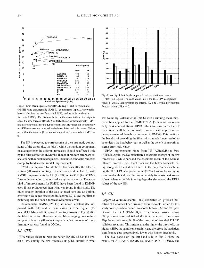
3.2. RMSE

Following Wilmott (1981) we decompose RMSE into systematic

(RMSEs) and unsystematic (RMSEu) (i.e. random) components

to better understand the KF correction effects on the forecast

skill (see DM06b for a detail description of Willmott’s decom-

position). RMSEs indicates the portion of error that depends

on model systematic errors (e.g. inaccurate model parameters),

while RMSEu depends on random errors and on errors resulting

by a model skill deficiency in predicting a specific situation (e.g.

a process not described in the model formulation). The following

relationship holds between RMSE and its components:

RMSE2 = RMSE2s + RMSE2

u . (7)

Figure 5 is built using the forecasts RMSE, RMSEs and RMSEu .

Each arrow tail has as abscissa the raw forecast RMSEs and as

ordinate the raw forecast RMSEu . This point distance from the

origin is equal to the raw forecast RMSE. Similarly, the arrow

head depicts RMSE and its components for the KF forecasts.

RMSE values for both the raw and KF forecasts are reported

in Fig. 5 lower right-hand corner. If an arrow is pointing to the

left-hand side it means KF is reducing the forecast RMSEs , and

if it is pointing downward is reducing RMSEu .

The closer the values of these metrics are to zero the bet-

ter. RMSE is improved (lower values) for all the determinis-

tic forecasts. E is also improved after the correction, while EK

filtered version has a higher RMSE. Among the raw forecasts

WRF/CHEM-2 has the lowest RMSE, while the best overall is

again the unfiltered EK. Also with this metric double filtering did

not provide any improvement as reported in DM06b. Ensemble

averaging and Kalman filtering when combined together, regard-

less of the order on which these operators are applied, provide

the best forecast overall (lowest RMSE).

Tellus 60B (2008), 2

244 L. DELLE MONACHE ET AL.

0 2 4 6 8 10 12 14 16 18 20 22 24 26 28 30 32 340

2

4

6

8

10

12

14

16

18

20

22

24

AURAMS

AURAMS 17.5 15.9

18.2 14

BAMS 45

BAMS 45 19.2 15

CHRONOS

CHRONOS 23.2 17.7

CMAQ/ETA

CMAQ/ETA 21.5 13.5

WRF/CHEM 1

WRF/CHEM 1 22 15.1

WRF/CHEM 2

WRF/CHEM 2 16.6 13.8

STEM

STEM 37.4 19.4

E

E 18.1 11.5

EK

EK 11.2 12.7

RMSE Systematic (ppbv)

RM

SE

U

ns

ys

tem

ati

c (

pp

bv

)

RMSE (ppbv)

Raw KF

Fig. 5. Root mean square error (RMSE) (eq. 4) and its systematic

(RMSEs ) and unsystematic (RMSEu ) components (ppbv). Arrow tails

have as abscissa the raw forecasts RMSEs and as ordinate the raw

forecasts RMSEu . The distance between the arrow tail and the origin is

equal the raw forecast RMSE. Similarly, the arrow head depicts RMSE

and its components for the KF forecasts. RMSE values for both the raw

and KF forecasts are reported in the lower left-hand side corner. Values

are within the interval [0, +∞), with a perfect forecast when RMSE =0.

The KF is expected to correct some of the systematic compo-

nents of the errors (i.e. the bias), while the random component

on average (over the different forecasts) should be affected little

by the filter correction (DM06b). In fact, if random errors are as-

sociated with model inadequacies, then those cannot be removed

except by fundamental model improvements.

RMSEs is improved for all the 10 forecasts after the KF cor-

rection (all arrows pointing to the left-hand side in Fig. 5), with

RMSEs improvements by 1% (for EK) up to 82% (for STEM).

Ensemble averaging does not reduce systematic error. The same

kind of improvements for RMSEs have been found in DM06b,

even if less pronounced than what was found in this study. The

much greater duration of the data set used here and an optimal

error-ratio value (as discussed in Section 2.2) allow the filter to

better capture the ozone-forecast systematic errors.

Unsystematic RMSE(RMSEu) is never substantially im-

proved with KF, and in few cases is even higher (for

WRF/CHEM-2 and EK, upward pointing arrows in Fig. 5) after

the filter correction. However, ensemble averaging does reduce

unsystematic error (filters out unpredictable components), con-

firming what was found in DM06b.

3.3. UPPA

UPPA values closer to zero are better. BAMS-15 has the low-

est UPPA among the raw forecasts (Fig. 6), similar to what

10

15

20

25

30

35

40

45

50

55

60

65

UP

PA

(%

)

AURAMS

BAMBAM

CHRONOS

CMAQ/ETA

WRF/CHEM

WRF/CHEM STEM E EK

Fig. 6. As Fig. 4, but for the unpaired peak prediction accuracy

(UPPA) (%) (eq. 5). The continuous line is the U.S. EPA acceptance

values (+20%). Values within the interval [0, +∞), with a perfect peak

forecast when UPPA = 0.

was found by Wilczak et al. (2006) with a running-mean bias-

correction applied to the ICARTT/NEAQS data set for ozone

daily peak concentrations. UPPA values are lower after the KF

correction for all the deterministic forecasts, with improvements

more pronounced than those presented in DM06b. This confirms

the benefits of providing the filter with a much longer period to

better learn the bias behaviour, as well as the benefit of an optimal

sigma error-ratio value.

UPPA improvements range from 7% (AURAMS) to 50%

(STEM). Again, the Kalman filtered ensemble average of the raw

forecasts (E, white bar) and the ensemble mean of the Kalman

filtered forecasts (EK, black bar) are the better forecasts be-

ing, along with the Kalman filter EK, the only forecasts achiev-

ing the U.S. EPA acceptance value (20%). Ensemble-averaging

combined with Kalman filtering accurately forecasts peak ozone

values, whereas double filtering degrades (increases) the UPPA

values of the raw EK.

3.4. CSI

Larger CSI values (closer to 100%) are better. CSI gives an indi-

cation of the forecast performance for rare events, which for this

study corresponds to ozone thresholds between 60 and 90 ppbv.

During the ICARTT/NEAQS experiments, ozone above

60 ppbv was observed 6% of the time, whereas ozone above

90 ppbv was observed 0.1% of the time, out of a total of 421 082

valid observations. This means that the higher the threshold, the

higher will be the sample uncertainty, and therefore the statistical

significance gets progressively lower with higher thresholds.

The five panels on the left-hand side in Fig. 7 show the

results for AURAMS, BAMS-15, BAMS-45, CHRONOS and

Tellus 60B (2008), 2

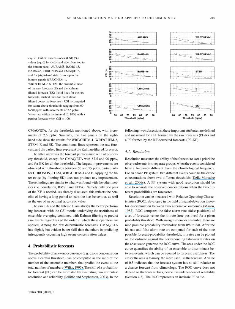
KF BIAS CORRECTION METHOD APPLIED TO DETERMINISTIC 245

01020304050

AURAMS

01020304050

01020304050

CS

I (%

)

01020304050

CHRONOS

60 65 70 75 80 85 900

1020304050

CMAQ/ETA

Threshold (ppbv)

STEM

E

60 65 70 75 80 85 90

EK

Threshold (ppbv)

Fig. 7. Critical success index (CSI) (%)

values (eq. 6) for (left-hand side: from top to

the bottom panel) AURAMS, BAMS-15,

BAMS-45, CHRONOS and CMAQ/ETA

and for (right-hand side: from top to the

bottom panel) WRF/CHEM-1,

WRF/CHEM-2, STEM, the ensemble mean

of the raw forecasts (E) and the Kalman

filtered forecast (EK) (solid lines for the raw

forecasts, dashed lines for the Kalman

filtered corrected forecasts). CSI is computed

for ozone above thresholds ranging from 60

to 90 ppbv, with increments of 2.5 ppbv.

Values are within the interval [0, 100], with a

perfect forecast when CSI = 100.

CMAQ/ETA, for the thresholds mentioned above, with incre-

ments of 2.5 ppbv. Similarly, the five panels on the right-

hand side show the results for WRF/CHEM-1, WRF/CHEM-2,

STEM, E and EK. The continuous lines represent the raw fore-

cast, and the dashed lines represent the Kalman-filtered forecasts.

The filter improves the forecast performance with almost ev-

ery threshold, except for CMAQ/ETA with 87.5 and 90 ppbv,

and for EK for all the thresholds. The largest improvements are

observed with thresholds between 60 and 75 ppbv, particularly

for CHRONOS, STEM, WRF/CHEM-1 and E. Applying the fil-

ter twice (by filtering EK) does not produce any improvement.

These findings are similar to what was found with the other met-

rics (i.e. correlation, RMSE and UPPA). Namely only one pass

of the KF is needed. As already discussed, this reflects the ben-

efits of having a long period to learn the bias behaviour, as well

as the use of an optimal error-ratio value.

The raw EK and the filtered E are always the better perform-

ing forecasts with the CSI metric, underlying the usefulness of

ensemble averaging combined with Kalman filtering to predict

rare events regardless of the order in which these operators are

applied. Among the raw deterministic forecasts, CMAQ/ETA

has slightly but evident better skill than the others in predicting

infrequently occurring high ozone concentration values.

4. Probabilistic forecasts

The probability of an event occurrence (e.g. ozone concentration

above a certain threshold) can be computed as the ratio of the

number of the ensemble members that predict the event to the

total number of members (Wilks, 1995). The skill of a probabilis-

tic forecast (PF) can be estimated by evaluating two attributes:

resolution and reliability (Jolliffe and Stephenson, 2003). In the

following two subsections, these important attributes are defined

and measured for a PF formed by the raw forecasts (PF-R) and

a PF formed by the KF-corrected forecasts (PF-KF).

4.1. Resolution

Resolution measures the ability of the forecast to sort a priori the

observed events into separate groups, when the events considered

have a frequency different from the climatological frequency.

For an ozone PF system, two different events could be the ozone

concentrations above two different thresholds (Delle Monache

et al., 2006c). A PF system with good resolution should be

able to separate the observed concentrations when the two dif-

ferent probabilities are forecasted.

Resolution can be measured with Relative Operating Charac-

teristics (ROC), developed in the field of signal-detection theory

for discrimination between two alternative outcomes (Mason,

1982). ROC compares the false alarm rate (false positives) of

a set of forecasts versus the hit rate (true positives) for a given

probability threshold. With an eight-member ensemble, there are

nine possible probability thresholds: from 0/8 to 8/8. After the

hit rate and false alarm rate are computed for each of the nine

possible forecast-probability thresholds, hit rates can be plotted

on the ordinate against the corresponding false-alarm rates on

the abscissa to generate the ROC curve. The area under the ROC

curve quantifies the ability of an ensemble to discriminate be-

tween events, which can be equated to forecast usefulness. The

closer the area is to unity, the more useful is the forecast. A value

of 0.5 indicates that the forecast system has no skill relative to

a chance forecast from climatology. The ROC curve does not

depend on the forecast bias, hence it is independent of reliability

(Section 4.2). The ROC represents an intrinsic PF value.

Tellus 60B (2008), 2

246 L. DELLE MONACHE ET AL.

10 20 30 40 50 60 70 80 900.6

0.65

0.7

0.75

0.8

0.85

0.9

0.95

1

Concentration Threshold (ppbv)

RO

C A

rea

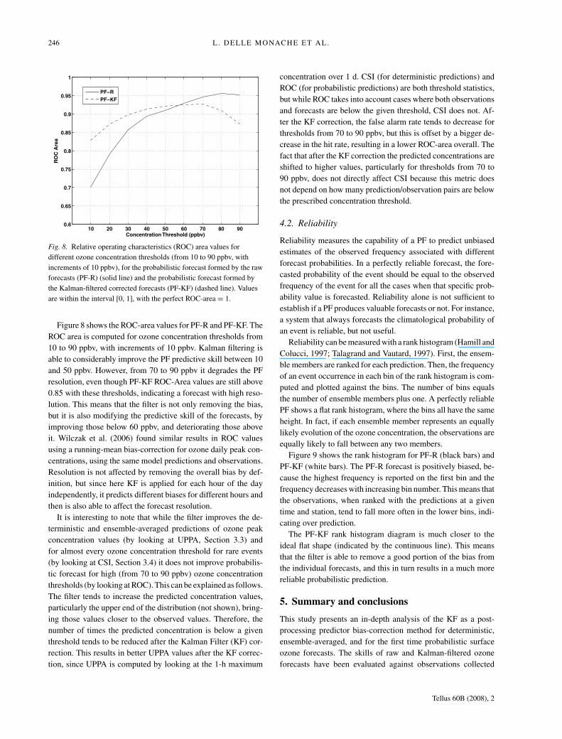
Fig. 8. Relative operating characteristics (ROC) area values for

different ozone concentration thresholds (from 10 to 90 ppbv, with

increments of 10 ppbv), for the probabilistic forecast formed by the raw

forecasts (PF-R) (solid line) and the probabilistic forecast formed by

the Kalman-filtered corrected forecasts (PF-KF) (dashed line). Values

are within the interval [0, 1], with the perfect ROC-area = 1.

Figure 8 shows the ROC-area values for PF-R and PF-KF. The

ROC area is computed for ozone concentration thresholds from

10 to 90 ppbv, with increments of 10 ppbv. Kalman filtering is

able to considerably improve the PF predictive skill between 10

and 50 ppbv. However, from 70 to 90 ppbv it degrades the PF

resolution, even though PF-KF ROC-Area values are still above

0.85 with these thresholds, indicating a forecast with high reso-

lution. This means that the filter is not only removing the bias,

but it is also modifying the predictive skill of the forecasts, by

improving those below 60 ppbv, and deteriorating those above

it. Wilczak et al. (2006) found similar results in ROC values

using a running-mean bias-correction for ozone daily peak con-

centrations, using the same model predictions and observations.

Resolution is not affected by removing the overall bias by def-

inition, but since here KF is applied for each hour of the day

independently, it predicts different biases for different hours and

then is also able to affect the forecast resolution.

It is interesting to note that while the filter improves the de-

terministic and ensemble-averaged predictions of ozone peak

concentration values (by looking at UPPA, Section 3.3) and

for almost every ozone concentration threshold for rare events

(by looking at CSI, Section 3.4) it does not improve probabilis-

tic forecast for high (from 70 to 90 ppbv) ozone concentration

thresholds (by looking at ROC). This can be explained as follows.

The filter tends to increase the predicted concentration values,

particularly the upper end of the distribution (not shown), bring-

ing those values closer to the observed values. Therefore, the

number of times the predicted concentration is below a given

threshold tends to be reduced after the Kalman Filter (KF) cor-

rection. This results in better UPPA values after the KF correc-

tion, since UPPA is computed by looking at the 1-h maximum

concentration over 1 d. CSI (for deterministic predictions) and

ROC (for probabilistic predictions) are both threshold statistics,

but while ROC takes into account cases where both observations

and forecasts are below the given threshold, CSI does not. Af-

ter the KF correction, the false alarm rate tends to decrease for

thresholds from 70 to 90 ppbv, but this is offset by a bigger de-

crease in the hit rate, resulting in a lower ROC-area overall. The

fact that after the KF correction the predicted concentrations are

shifted to higher values, particularly for thresholds from 70 to

90 ppbv, does not directly affect CSI because this metric does

not depend on how many prediction/observation pairs are below

the prescribed concentration threshold.

4.2. Reliability

Reliability measures the capability of a PF to predict unbiased

estimates of the observed frequency associated with different

forecast probabilities. In a perfectly reliable forecast, the fore-

casted probability of the event should be equal to the observed

frequency of the event for all the cases when that specific prob-

ability value is forecasted. Reliability alone is not sufficient to

establish if a PF produces valuable forecasts or not. For instance,

a system that always forecasts the climatological probability of

an event is reliable, but not useful.

Reliability can be measured with a rank histogram (Hamill and

Colucci, 1997; Talagrand and Vautard, 1997). First, the ensem-

ble members are ranked for each prediction. Then, the frequency

of an event occurrence in each bin of the rank histogram is com-

puted and plotted against the bins. The number of bins equals

the number of ensemble members plus one. A perfectly reliable

PF shows a flat rank histogram, where the bins all have the same

height. In fact, if each ensemble member represents an equally

likely evolution of the ozone concentration, the observations are

equally likely to fall between any two members.

Figure 9 shows the rank histogram for PF-R (black bars) and

PF-KF (white bars). The PF-R forecast is positively biased, be-

cause the highest frequency is reported on the first bin and the

frequency decreases with increasing bin number. This means that

the observations, when ranked with the predictions at a given

time and station, tend to fall more often in the lower bins, indi-

cating over prediction.

The PF-KF rank histogram diagram is much closer to the

ideal flat shape (indicated by the continuous line). This means

that the filter is able to remove a good portion of the bias from

the individual forecasts, and this in turn results in a much more

reliable probabilistic prediction.

5. Summary and conclusions

This study presents an in-depth analysis of the KF as a post-

processing predictor bias-correction method for deterministic,

ensemble-averaged, and for the first time probabilistic surface

ozone forecasts. The skills of raw and Kalman-filtered ozone

forecasts have been evaluated against observations collected

Tellus 60B (2008), 2

KF BIAS CORRECTION METHOD APPLIED TO DETERMINISTIC 247

1 2 3 4 5 6 7 8 90

0.05

0.1

0.15

0.2

0.25

0.3

0.35

0.4

Bin (i.e., Interval Index)

Fre

qu

en

cy

Fig. 9. Rank histogram for the probabilistic forecast formed by the raw

forecasts (PF-R) (black bars) and the probabilistic forecast formed by

the Kalman-filtered corrected forecasts (PF-KF) (white bars). The

number of bins equals the number of ensemble members plus one. The

solid horizontal line represents the perfect rank histogram shape (flat).

The closer is the diagram to this horizontal line, the better is the

reliability of the probabilistic forecast.

during the summer 2004 in the Northeast United States and

Southeast Canada, as part of the International Consortium for

Atmospheric Research on Transport and Transformation/New

England Air Quality Study (ICARTT/NEAQS) (McKeen et al.,

2005). The completeness of this data set, including 1-h ozone

forecasts from eight different simulations for 56 d, and observa-

tions from roughly 360 stations, offered a unique opportunity to

thoroughly test the filter performance. However, the summer of

2004 exhibited very few occurrences of pollution episodes be-

cause it was unseasonably cool. The statistics presented in this

study are therefore specific to the summer of 2004 and might not

be climatologically representative.

An optimal KF error-ratio parameter value of 0.4 has been

found by evaluating the filter performance in different situa-

tions with different meteorology and different air quality (AQ)

scenarios. This optimal value considerably inproved the KF per-

formance compared to its performance with the error ratio value

found in Delle Monache et al., 2006b (hereinafter referred to

as DM06b), and is therefore likely to produce a better KF per-

formance for future real-time surface ozone forecasts. However,

a search of the KF optimal ratio value by analysing a data set

including more typical ozone episodes may result in a different

value from what has been found in this study.

Kalman filtering significantly improves the correlation (i.e. the

linear dependency) between the predicted and measured ozone

time series for all the forecasts [except for the Canadian Hemi-

spheric and Regional Ozone and NOx System (CHRONOS), and

the filtered ensemble mean of the KF forecasts (EK)]. A lead/lag

correlation analysis also showed that the KF-corrected ozone

forecasts result in an improved accuracy in predicting the timing

of concentration peak and minimum values. The forecasts hav-

ing the best overall correlation are EK and the Kalman-filtered

ensemble average of the raw forecasts (E). For raw deterministic

forecasts the Weather Research and Forecast Model/Chemistry

model version 2.03 (WRF/CHEM-2) has the best correlation,

although still less than EK and E. Ensemble averaging increases

the correlation with the observations for both raw and filtered

forecasts.

For all the deterministic forecasts, the KF improves the abil-

ity to predict the ozone-concentration magnitude [based on the

root mean square error (RMSE)]. Among the raw forecasts

WRF/CHEM-2 has the lowest RMSE, while the best RMSE

overall is again for the raw EK and the filtered E. The tests in-

volving RMSE systematic (RMSEs) and unsystematic (RMSEu)

components confirmed the results in DM06b: the filter removes

a good portion of the bias while it has a minimal affects on the

random errors. Vice versa, ensemble averaging tends to remove

the unsystematic component of RMSE, while it leaves substan-

tially unaltered the bias. For this reason (considering also the

other statistical metrics), the combination of Kalman filtering

and ensemble averaging (i.e. EK) or vice versa (i.e. the filtered

E), resulted in the best forecasts in this study.

KF improves the ability to predict the daily surface ozone

maximum concentration magnitude. Comparing the unpaired

peak prediction accuracy (UPPA) metric results, the filtered

EK has the lowest (best) value, while Baron Advanced Me-

teorological System Multi-scale Air Quality Simulation Plat-

form run at 15 km (BAMS-15) has the lowest UPPA among the

raw deterministic forecasts (similar to what found by Wilczak

et al. (2006) using a running-mean bias-correction for the

ozone maximum predictions with the ICARTT/NEAQS data

set). E filtered, EK, and EK filtered are the only forecasts hav-

ing UPPA values of sufficiently high accuracy that they are

within the U.S. Environmental Protection Agency (EPA) ac-

ceptance value (120%, U.S. Environmental Protection Agency,

1991). This suggests the necessity of ensemble-averaging and

Kalman filtering to accurately forecast the surface ozone peak

magnitude.

Kalman filtering also improves the ability to predict most

rare events as measured by the Critical Success Index (CSI).

EK and the filtered E are always better than the other forecasts

in forecasting these low-frequency events, demonstrating also

in these cases the usefulness of ensemble averaging combined

with Kalman filtering. The Community Multi-scale Air Quality

Model (CMAQ/ETA) has the highest CSI values among the raw

deterministic forecasts.

Kalman filtering is able to improve considerably the

probabilistic-forecast (PF) predictive skill for ozone concentra-

tions above thresholds from 10 to 50 ppbv. However, from 70 to

90 ppbv it degrades the PF resolution, even though the ROC-Area

values are still above 0.85 with these two thresholds, indicating a

forecast with high resolution. Wilczak et al. (2006) found similar

results in ROC values using a running-mean bias-correction for

Tellus 60B (2008), 2

248 L. DELLE MONACHE ET AL.

ozone daily peak concentrations with the ICARTT/NEAQS data

set.

The rank histograms show that the PF composed by raw fore-

casts is positively biased, whereas PF including the Kalman

filtered forecasts is much closer to the ideal flat shape, mean-

ing that the filter removes successfully most of the bias from

the individual forecasts, and this in turn results in a much more

reliable probabilistic prediction.

Finally, the results of this study indicate that only one applica-

tion of the KF is needed to achieve the best correction (compared

to earlier findings by DM06b suggesting that two applications of

the filter are useful). This reflects the benefits of having a longer

period to learn the bias behaviour (as with the ICARTT/NEAQS

data set used here), as well as the use of an optimal error-ratio

value.

The significance of KF post-processing and ensemble averag-

ing is that they are both effective for real-time AQ forecasting.

Namely, they reduce both systematic biases and random errors

from coupled meteorological and Chemistry Transport Models

(CTMs) to give the best estimate of future conditions, regard-

less of the synoptic situation and for AQ scenarios for which the

underlying models were not specifically tuned.

In this work KF has been applied to improve photochemical

model predictions of surface ozone. Those models are also used

to produce efficient ozone controlling strategies, where different

emission scenarios are considered to understand which action

(e.g. anthropogenic emission reduction) would be most benefi-

cial to reduce ozone concentrations. It is not obvious how KF

could be also used for such applications and this task is left to

future investigations.

6. Acknowledgments

This research is partially funded by Early Start Funding

from the NOAA/NWS Office of Science and Technology

and the NOAA Office of Atmospheric Research Weather

and Air Quality Program and would not be possible with-

out the participation of the AIRNow program and participat-

ing stakeholders. Credit for program support and management

is given to Paula Davidson (NOAA/NWS/OST), Steve Fine

(NOAA/ESRL/CSD), and Jim Meagher (NOAA/ESRL/CSD).

Computational and logistic assistance from the following in-

dividuals and organizations is also gratefully appreciated:

Amenda Stanley (NOAA/ESRL/GSD), Ted Smith (Baron

AMS), Jessica Koury (NOAA/ESRL/PSD), Wendi Madsen

(NOAA/ESRL/PSD), Ann Keane (NOAA/ESRL/PSD), Sophie

Cousineau (MSC), L.-P. Crevier (MSC), Stephane Gaudreault

(MSC), Mike Moran (AQRB/MSC), Paul Makar (AQRB/MSC),

Balbir Pabla (AQRB/MSC), Dezso Devenyi (FSL/NOAA) and

the NOAA/ESRL/GSD High Performance Computing Facility.

The authors thank Veronique Bouchet for being instrumental in

making the CHRONOS model output available. Thanks are also

due to three anonymous reviewers for providing useful com-

ments and suggestions. Luca Delle Monache’s work was per-

formed under the auspices of the U.S. Department of Energy by

Lawrence Livermore National Laboratory under Contract DE-

AC52-07NA27344.

References

Atkinson, R., Baulch, D. L., Cox, R. A., Hampson, R. F., Kerr, J. A.

and co-authors. 1992. Evaluated kinetic and photochemical data for

atmospheric chemistry: supplement IV. Atmos Environ. 26A, 1187–

1230.

Binkowski, F. S. and Shankar, U. 1995. The regional particulate model. I.

Model description and preliminary results. J. Geophys. Res. 100(D12),

26191–26209.

Bozic, S. M. 1994. Digital and Kalman Filtering 2nd

Edition.Butterworth-Heinemann, New York, 160 pp.

Byun, D. W. and Schere, K. L. 2006. Description of the Models-3 Com-

munity Multiscale Air Quality (CMAQ) Model: system overview, gov-

erning equations, and science algorithms. Appl. Mech. Rev. 59, 51–77.

Carmichael, G. R., Tang, Y., Kurata, G., Uno, I., Streets, D. and co-

authors. 2003. Regional-scale chemical transport modeling in support

of the analysis of observations obtained during the TRACE-P experi-

ment. J. Geophys. Res. 108(D21), 8823, doi:10.1029/2002JD003117.

Carter, W. 2000. Documentation of the SAPRC-99 chemical mech-

anism for VOC reactivity assessment. Final Report to California

Air Resources Board Contract No. 92-329, University of California,

Riverside.

Cote, J., Gravel, S., Methot, A., Patoine, A., Roch, M. and co-authors.

1998a. The operational CMC-MRB Global Environmental Multiscale

(GEM) model. Part I: design considerations and formulation. Mon.Wea. Rev. 126, 1373–1395.

Cote, J., Desmarais, J.-G., Gravel, S., Methot, A., Patoine, A. and

co-authors. 1998b. The operational CMC/MRB Global Environmen-

tal Multiscale (GEM) model. Part II: results. Mon. Wea. Rev. 126,

1397–1418.

Delle Monache, L. and Stull, R. B. 2003. An ensemble air quality forecast

over western Europe during an ozone episode. Atmos. Environ. 37,

3469–3474.

Delle Monache, L., Deng, X., Zhou, Y. and Stull, R. B. 2006a. Ozone

ensemble forecasts: 1. A new ensemble design. J. Geophys. Res. 111,

D05307, doi:10.1029/2005JD006310.

Delle Monache, L., Nipen, T., Deng, X., Zhou, Y. and Stull, R. B. 2006b.

Ozone ensemble forecasts: 2. A Kalman-filter predictor bias correc-

tion. J. Geophys. Res. 111, D05308, doi:10.1029/2005JD006311.

Delle Monache, L., Hacker, J. P., Zhou, Y., Deng, X. and Stull,

R. B. 2006c. Probabilistic aspects of meteorological and ozone

regional ensemble forecasts. J. Geophys. Res. 111, D24307,

doi:10.1029/2005JD006917.

Gery, M. W., Whitten, G., Killus, J. and Dodge, M. 1989. A photochemi-

cal kinetics mechanism for urban and regional scale computer models.

J. Geophys. Res. 94, 12295–12356.

Grell, G. A., Dudhia, J. and Stauffer, D. R. 1994. A description of the

fifth-generation Penn State/NCAR Mesoscale Model (MM5). NCAR

Tech. Note, NCAR/TN-398+STR, 122 p.

Grell, G. A., Peckham, S. E., Schmitz, R., McKeen, S. A., Frost, G. and

co-authors. 2005. Fully coupled “online” chemistry within the WRF

model. Atmos. Environ. 39, 6957–6975.

Tellus 60B (2008), 2

KF BIAS CORRECTION METHOD APPLIED TO DETERMINISTIC 249

Hamill, T. and Colucci, S. J. 1997. Verification of Eta-RSM short-range

ensemble forecasts. Mon. Wea. Rev. 125, 1312–1327.

Hamill, T. M. and Snyder, C. 2000. A hybrid ensemble Kalman filter-3D

variational analysis scheme. Mon. Wea. Rev. 128, 2905–2919.

Homleid, M. 1995. Diurnal corrections of short-term surface temperature

forecasts using Kalman filter. Wea. Forecast. 10, 989–707.

Jolliffe, I. T. and Stephenson, D. B. 2003. Forecast Verification: A Prac-titioner’s Guide in Atmospheric Science (eds. I. I. Jolliffe and D. B.

Stephenson), Wiley and Sons, 240 p.

Lurman, F. W., Lloyd, A. C. and Atkinson, R. 1986. A chemical mech-

anism for use in long-range transport/acid deposition computer mod-

eling. J. Geophys. Res. 91, 10905–10936.

Mallet, V. and Sportisse, B. 2006. Ensemble-based air quality fore-

casts: A multimodel approach applied to ozone. J. Geophys. Res. 111,

D18302.

Mason, I. 1982. A model for assessment of weather forecasts. Aust.Meteor. Mag. 30, 291–303.

McHenry, J. N., Ryan, W. F., Seaman, N. L., Coats, C. J., Jr. Pudykiewicz,

J. and co-authors. 2004. A real-time Eulerian photochemical model

forecast system. Bull. Amer. Meteor. Soc. 85, 525–548.

McKeen, S. A., Wilczak, J. M., Grell, G. A., Djalalova, I., Peckham, S.

and co-authors. 2005. Assessment of an ensemble of seven real-time

ozone forecasts over Eastern North America during the summer of

2004. J. Geophys. Res. 110, D21307, doi:10.1029/2005JD005858.

McQueen, J. and co-authors. 2004. Development and evaluation of

the NOAA/EPA prototype air quality model prediction system. In:

Preprints, 20th Conference on Weather Analysis and Forecasting/16thConference on Numerical Weather Prediction, 12–15 January 2004,

Seattle, Washington, USA.

Moran, M. D., Scholtz, M. T., Slama, C. F., Dorkalam, A., Taylor, A.

and co-authors. 1997. An overview of CEPS1.0: version 1.0 of the

Canadian Emissions Processing System for regional-scale air quality

models. In: Proceedings of 7th AWMA Emission Inventory Symposium,

28–30 October 1997, Research Triangle Park, North Carolina, USA.

Pagowski, M., Grell, G. A., McKeen, S. A., Devenyi, D., Wilczak,

J. M. and co-authors. 2005. A simple method to improve

ensemble-based ozone forecasts. Geophys. Res. Lett. 32, L07814,

doi:10.1029/2004GL022305.

Pagowski, M., Grell, G. A., Devenyi, D., Peckham, S. E., McKeen, S.

A. and co-authors. 2006. Application of dynamic linear regression to

improve skill of ensemble-based deterministic ozone forecasts. Atmos.Environ. 40, 3240–3250.

Pudykiewicz, J., Kallaur, A. and Smolarkiewicz, P. K. 1997. Semi-

Lagrangian modeling of tropospheric ozone. Tellus 49B, 231–258.

Roeger, C., Stull, R. B., McClung, D., Hacker, J., Deng, X. and co-

authors. 2003. Verification of mesoscale numerical weather forecast

in mountainous terrain for application to avalanche prediction. Wea.Forecast. 18, 1140–1160.

Russell, A. and Dennis, R. 2000. NARSTO critical review of photochem-

ical models and modeling. Atmos. Environ. 34, 2283–2324.

Stockwell, W. R., Middleton, P., Chang, J. S. and Tang, X. 1995.

The effect of acetyl peroxy-pperoxy radical reactions on peroxy-

acetyl nitrate and ozone concentrations. Atmos. Environ. 29, 1591–

1599.

Talagrand, O. and Vautard, R. 1997. Evaluation of probalistic prediction

systems, Proceedings ECMWF Workshop on Predictability, ECMWF,Reading, UK, 1–25.

Thunis, P. and co-authors. 2007. Analysis of model responses to

emission-reduction scenarios with in the City Delta project. Atmos.Environ. 41, 208–220.

U.S. Environmental Protection Agency. 1991. Guideline for Regulatory

Application Of The Urban Airshed Model. USEPA Rep., EPA-450/4-91-013, Research Triangle Park, North Carolina, USA.

van Loon, M., Builtjes, P. J. H. and Segers, A. J. 2000. Data assimilation

applied to LOTOS: first experiences. Environ. Model. Software 15,

603–609.

van Loon, M. and co-authors. 2007. Evaluation of long-term ozone sim-

ulations from seven regional air quality models and their ensemble.

Atmos. Environ. 41, 2083–2097.

Wilczak, J. M., McKeen, S. A., Djalalova, I. and Grell, G. 2006. Bias-

corrected ensemble predictions of surface O3. J. Geophys. Res. 111,

D23S28, doi:10.1029/2006JD007598.

Wilks, D. S. 1995. Statistical Methods in the Atmospheric Sciences (eds.

R. Dmowska and J. R.Holton). Academic Press, 467 pp.

Willmott, C. J. 1981. On the validation of models. Phys. Geogr. 2, 184–

194.

Tellus 60B (2008), 2