A jump filter for uncertain dynamic systems with dropouts

A jump filter for uncertain dynamic systems with dropouts

D. Dolz, D. E. Quevedo, I. Penarrocha, and R. Sanchis

Abstract— In this work, we consider a state estimation prob-lem for linear uncertain discrete-time systems over a networkwith dropouts. The uncertainty of the plant model is describedby a norm-bounded time-varying parameter that affects thesystem matrix. We design a jump filter that minimizes an upperbound of the trace of the state estimation error covariancefor all possible parameter uncertainties and whose gains areselected from a precalculated finite set depending on the possi-ble measurement reception scenarios. The presented procedureallows us to relate the complexity of the jump filter to theachievable estimation performance.

I. INTRODUCTION

In the latest years, networked control systems, in which thecontroller unit, sensors and actuator are not collocated, havebeen widely extended in the industry due to the reduction onthe installation cost and the increase on the flexibility [9].However the use of a shared network to transmit the infor-mation, leads to some network-induced phenomena such aspacket dropouts and time delays [10], [3].

The networked estimation problem has been given a greatdeal of attention. The Kalman filter has been used to achieveoptimal performance at the expense of a considerable on-linecomputational effort [15], [14]. The pursuit of low imple-mentation cost options has led to the use of precalculatedgains from a finite set [16], [13]. This idea reduces theimplementation computing needs, only requiring the storageof the gains and the selection of the appropriate one ateach instant, at the expense of a reduction in the estimationperformance. Motivated by the use of low cost methods wewill only focus on the last alternative.

Unfortunately, the aforementioned methods will not guar-antee, in general, acceptable performance when the plantmodel has parameter uncertainties (which can be char-acterized e.g., with norm-bounded [20] or polytopic [2]structures). The aim in the estimation problem with modeluncertainties is to guarantee that the estimation error co-variance lies within a certain bound for all the possibleuncertainties [20], [6], [17].

Before presenting our current results, we will first give abrief overview of previous literature of interest. In [20], theauthors designed a predictor for the case when the state ma-trix is affected by constant norm-bounded uncertainties withmeasurement packetized dropouts described by a Bernoullisequence, while in [18] the uncertainties on the output matrix

D. Dolz , I. Penarrocha, and R. Sanchis are with Department of IndustrialSystem Engineering and Design, Universitat Jaume I of Castello, Spain{ddolz,ipenarro,rsanchis}@uji.es

D. E. Quevedo is with the School of Electrical Engineering andComputer Science, The University of Newcastle, NSW, [email protected]

were also included. The predictor design for time-varyingstate matrix uncertainty was conducted in [21].

The approaches in [20], [6], [18] are conservative in thesense of using a memoryless model of the network-induceddropout, and also, because of the adoption of a constantinvariant gain estimation scheme. Markovian jump modelscan represent more accurately the dropout phenomenon andallow to relate the estimator gains with the jump modes [16](the gains can also depend on the states of a Bernoulli pro-cess, e.g. [13]). The authors in [11], [7] study the predictordesign under time-varying and mode dependent uncertaintiesfor Markovian jump systems. However their jump modesdo not explicitly depend on the available measurements.Further, their design methods do not handle the inclusion ofdifferent gain dependency strategies to reduce the estimatorcomplexity.

In this current work we deal with the filter design prob-lem for multisensor uncertain systems under networks withunbounded dropouts. The uncertainty is modeled by a norm-bounded time-varying matrix that affects the state matrix.We model the network effects by a parameter that describesthe measurement outcomes at each instant following a fi-nite Markov chain. Based on this process, we design ajump linear estimator that is adapted to the transmissionoutcome. Our method minimizes an upper bound of thetrace of the state estimation error covariance for all possibleparameter uncertainties. The proposed method also dealswith the covariance-constrained approach proposed in [20],[18], where instead of the trace minimization, the stateestimation error covariance is constrained to lie under agiven bound. The current design allows for the search offavorable trade-offs between estimation performance and on-line computational implementation. Moreover, we study thecounterparts of constraining some filter gains to be equal fordifferent values of the measurement outcomes parameter.

This paper can be seen as an extension to uncertaindynamic systems of recent author’s work [5], [4]. Moreover,in this present work we consider more general dropoutscenarios than the one governed by a Bernoulli process.

The paper has the following structure. In Section II,we discuss the problem of concern. In Section III, wederive the conditions to guarantee stochastic stability and thefilter design. In Section IV we expose some gain groupingapproaches to reduce the implementation cost. Simulationstudies illustrate the results in Section V. Section VI drawsconclusions.

Notation and Basic Definitions: Let R denote the realnumbers set. Let A an B be some matrices and I be theidentity matrix. A � 0 means that matrix A is negative

semidefinite. Similar applies to ≺, � and �. The directsum is represented as

⊕, where A

⊕B is a block diagonal

matrix with A and B on its diagonal. Let L be a givenfinite set, |L| denotes its cardinality. Expected value andprobability are denoted as E{·} and Pr{·}

II. PROBLEM DESCRIPTION

Let us consider linear uncertain discrete-time systems ofthe form

x[t+ 1] = (A+ ∆A[t])x[t] +Bw[t], (1)y[t] = C x[t] + v[t], (2)

where x ∈ Rn is the state, u ∈ Rnu is the control input,y ∈ Rny is the measured output with y =

[y1 · · · yny

]Tand ys being measured with a different sensor (with s =1, . . . , ny). The state disturbance is denoted by w ∈ Rnw

and v ∈ Rny is the sensor noise. Both the disturbance andnoise are assumed mutually uncorrelated and independentGaussian signals with zero mean and known covarianceE{w[t]w[t]T } = W and E{v[t] v[t]T } = V . We considerthat the initial state x[0] is uncorrelated with both of w[t]and v[t]. Matrix A is assumed to be Schur stable.

II. PROBLEM DESCRIPTION

Let us consider linear uncertain discrete-time systems ofthe form

x[t+ 1] = (A+∆A[t])x[t] +Bw[t], (1)

y[t] = C x[t] + v[t], (2)

where x ∈ Rn is the state, u ∈ Rnu is the control input,y ∈ Rny is the measured output, w ∈ Rnw is the statedisturbance and v ∈ Rny is the sensor noise. Both thedisturbance and noise are assumed mutually uncorrelatedand independent gaussian signals with zero mean and knowncovariance E{w[t]w[t]T } = W and E{v[t] v[t]T } = V . Weconsider that the initial state x[0] is uncorrelated with bothof w[t] and v[t]. Matrix A is assumed to be Schur stable.

Filter

x[t]

UncertainPlant

Network

dropouts

•••

m1[t]

mny [t]

transmission outcome

y[t]

m[t], θ[t]

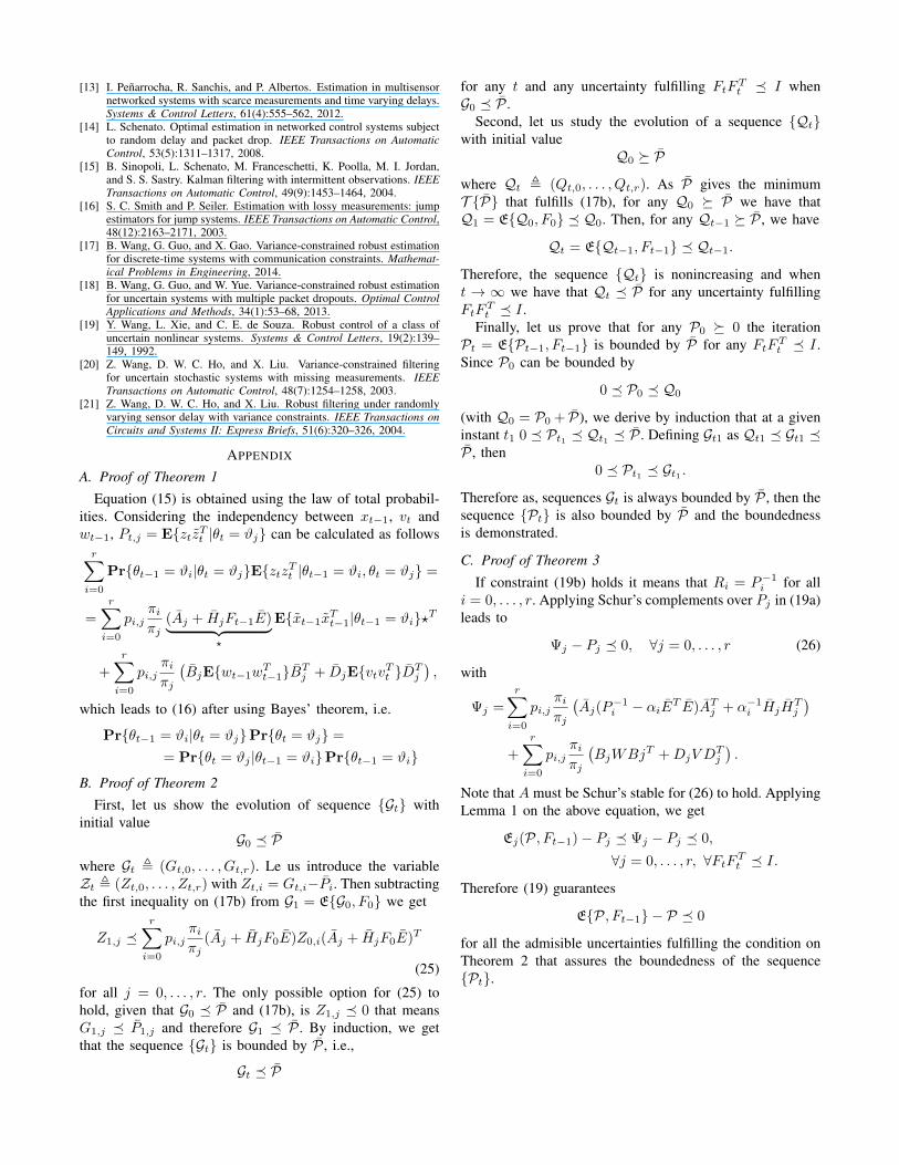
Fig. 1. Networked state estimator.

Matrix ∆A[t] is a real-valued time-varying matrix that rep-resents the parametric uncertainty affecting the state matrixand satisfying

∆A[t] = HF [t]E, F [t]F [t]T � I (3)

where H and E are known constant matrices of appropriatedimensions while F [t] is an unknown but bounded time-varying matrix.

A. Network modeling

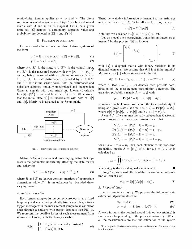
Each sensor samples its output synchronously with the in-put update and sends, independently from each other, a time-tagged message with the measurement sample to an estimatornode through a network with packet dropouts (see Fig. 1).We represent the possible losses of each measurement fromsensor s = 1 to ny with the binary variable

θs[t] =

{1 if ys[t] is received at instant t

0 if ys[t] is lost.(4)

Then, the available information at instant t at the estimatorunit is the pair (ms[t], θs[t]) for all s = 1, . . . , ny, where

ms[t] = θs[t] ys[t]. (5)

Note that we consider ms[t] = 0 if ys[t] is lost.Let us model the measurement transmission outcomes at

instant t by the process θ[t] as follows:

θ[t] =

ny⊕

s=1

θs[t], (6)

with θ[t] a diagonal matrix with binary variables in itsdiagonal elements. We assume that θ[t] is a finite ergodic1

Markov chain [1] whose states are in the set

θ[t] ∈ Θ = {ϑ0, ϑ1, . . . , ϑr}, r = 2ny − 1, (7)

where ϑi (for i = 0, . . . , r) denotes each possible combina-tion of the measurement transmission outcomes. The transi-tion probability matrix Λ = [pi,j ] with pi,j = Pr{θ[t+1] =ϑj

∣∣θ[t] = ϑi} is assumed to be know. We denote the totalprobability of being at a given state i as πi[t] = Pr{θ[t] =ϑi}, where π[t] = [π1[t], . . . , πr[t]] and π[t+ 1] = π[t]Λ.

Remark 1: If we assume an independent Markovainpacket dropout for each sensor transmission such that

Pr{θs[t] = 0|θs[t− 1] = 0} = qs,

Pr{θs[t] = 1|θs[t− 1] = 0} = 1− qs,

Pr{θs[t] = 1|θs[t− 1] = 1} = ps,

Pr{θs[t] = 0|θs[t− 1] = 1} = 1− ps,

then, each element of the transition probability matrix Λ =[pi,j ] of θt for i, j = 0, . . . , r is calculated as

pi,j =

ny∏

s=1

Pr{θs[t] = ϑs,j |θs[t− 1] = ϑs,i}

where ϑs,i is the s-th diagonal element of ϑi. �Using θ[t], we rewrite the available measurement informa-

tion at instant t as

m[t] = θ[t] (Cx[t] + v[t]) . (8)

B. Proposed filter

Let us rewrite x[t] as xt. We propose the following stateestimation algorithm

xt− = A xt−1 (9a)

xt = xt− + Lt(mt − θtCxt−), (9b)

At each instant t, the nominal model (without uncertainty) isrun in open loop, leading to the prior estimation xt− . Whenall the measurements are lost, the best estimation of thesystem state is the prior estimation, i.e., xt = xt− . Otherwise,the estimation state is updated using the updating gain matrixLt .

Considering (1) and (8)-(9), the dynamic of the estimationerror is xt = xt − xt, is

xt = (I−LtθtC) (Axt−1 +∆At−1xt−1 +Bwt−1)−Ltθtvt.(10)

We aim to calculate the gain matrices Lt that minimize thestate estimation error for all the admisible uncertainties whilerequiring low implementation resources. Thus, we relate thegains with θt, as Lt = L(θt), with the following law

L(θt) =

{0 if θt = ϑ0, (all measurements lost)

Li if θt = ϑi, i = 1, . . . , r.(11)

1In an ergordic Markov chain every state can be reached from every statein a finite time.

Fig. 1. Networked state estimation structure.

Matrix ∆A[t] is a real-valued time-varying matrix that rep-resents the parametric uncertainty affecting the state matrixand satisfying

∆A[t] = HF [t]E, F [t]F [t]T � I (3)

where H and E are known constant matrices of appropriatedimensions while F [t] is an unknown but bounded time-varying matrix.

A. Network modeling

Each sensor samples its output synchronously at a fixedfrequency and sends, independently from each other, a time-tagged message with the measurement sample to an estimatornode through a network with packet dropouts (see Fig. 1).We represent the possible losses of each measurement fromsensor s = 1 to ny with the binary variable

θs[t] =

{1 if ys[t] is received at instant t0 if ys[t] is lost.

(4)

Then, the available information at instant t at the estimatorunit is the pair (ms[t], θs[t]) for all s = 1, . . . , ny , where

ms[t] = θs[t] ys[t]. (5)

Note that we consider ms[t] = 0 if ys[t] is lost.Let us model the measurement transmission outcomes at

instant t by the process θ[t] as follows:

θ[t] =

θ1[t]θ2[t]

. . .θny[t]

, (6)

with θ[t] a diagonal matrix with binary variables in itsdiagonal elements. We assume that θ[t] is a finite ergodic1

Markov chain [1] whose states are in the set

θ[t] ∈ Θ = {ϑ0, ϑ1, . . . , ϑr}, r = 2ny − 1, (7)

where ϑi (for i = 0, . . . , r) denotes each possible com-bination of the measurement transmission outcomes. Thetransition probability matrix Λ = [pi,j ] with

pi,j = Pr{θ[t+ 1] = ϑj∣∣θ[t] = ϑi}

is assumed to be known. We denote the total probability ofbeing at a given state i at time t as πi[t] = Pr{θ[t] = ϑi},where π[t] = [π1[t], . . . , πr[t]] and π[t+ 1] = π[t]Λ.

Remark 1: If we assume mutually independent Markovianpacket dropouts for sensor transmissions such that

Pr{θs[t] = 0|θs[t− 1] = 0} = qs,

Pr{θs[t] = 1|θs[t− 1] = 0} = 1− qs,Pr{θs[t] = 1|θs[t− 1] = 1} = ps,

Pr{θs[t] = 0|θs[t− 1] = 1} = 1− ps,for all s = 1 to s = ny then, each element of the transitionprobability matrix Λ = [pi,j ] of θt for i, j = 0, . . . , r iscalculated as

pi,j =

ny∏

s=1

Pr{θs[t] = ϑs,j |θs[t− 1] = ϑs,i}

where ϑs,i is the s-th diagonal element of ϑi. �Using θ[t], we rewrite the available measurement informa-

tion at instant t as

m[t] = θ[t] (Cx[t] + v[t]) . (8)

B. Proposed filter

Let us rewrite x[t] as xt. We propose the following stateestimation algorithm structure

xt− = A xt−1 (9a)xt = xt− + Lt(mt − θtCxt−), (9b)

At each instant t, the nominal model (without uncertainty) isrun in open loop, leading to the prior estimation xt− . Whenall the measurements are lost, the estimation of the system

1In an ergordic Markov chain every state can be reached from every statein a finite time.

state is the prior estimation, i.e., xt = xt− . Otherwise, theestimation state is updated using the updating gain matrixLt .

Considering (1) and (8)-(9), the dynamic of the estimationerror is xt = xt − xt, is

xt = (I−LtθtC) (Axt−1 + ∆At−1xt−1 +Bwt−1)−Ltθtvt.(10)

We aim to calculate the gain matrices Lt that minimizethe state estimation error for all the admisible uncertaintieswhile requiring low implementation resources. We relate thegains with θt, as Lt = L(θt), with the following law

L(θt) =

{0 if θt = ϑ0, (all measurements lost)

Li if θt = ϑi, i = 1, . . . , r.(11)

The matrices are computed off-line leading to the finite set

L(θt) ∈ L = {L0, . . . , Lr}. (12)

To study this estimator it is convenient to introduce therandom process zt =

[xTt xTt

]T. Its dynamics is governed

byzt = (At + HtFt−1E)zt−1 + Btwt + Dtvt (13)

with

At =

[A 00 (I − LtθtC)A

], Ht =

[H

(I − LtθtC)H

],

E =[E 0

], Bt =

[B

(I − LtθtC)B

], Dt =

[0

−Ltθt

].

We will next show how to design a filter to obtain a boundedstate covariance matrix (in the steady state, i.e, when t→∞)for all the admisible uncertainties.

III. MAIN RESULTS

The Markov chain {θt} has a stationary distribution thatsatisfies π = πΛ because of its ergodicity. We assume theinitial condition π0 = π, and in consequence πt = π ∀t.Based on this assumption, the following result expresses theevolution of the state covariance matrix of (13).

Theorem 1: Let Pt−1,i = E{zt−1zTt−1|θt−1 = ϑi}, withi = 1, . . . , r, be the state covariance matrix of z at instantt− 1 given the measurement scenario θt−1 = ϑi. Theexpected value of the state covariance matrix at instant t,E{ztzTt }, is given by

r∑

j=0

E{ztzTt |θ[t] = ϑj}Pr{θ[t] = ϑj} =

r∑

j=0

πjPt,j , (15)

where

Pt,j =

r∑

i=0

pi,jπiπj

(Aj + HjFt−1E)Pt−1,i(Aj + HjFt−1E)T

+r∑

i=0

pi,jπiπj

(BjWBT

j + DjV DTj

), (16)

Proof: See Appendix A.Remark 2: The second diagonal element of Pt,j corre-

sponds to the state estimation error covariance matrix. It isgiven by CxPt,jC

Tx , with Cx =

[0 I

]. �

The above theorem states a recursion for the covariancematrix that depends on the value of the uncertain parameterFt. We thus write

Pt = E{Pt−1, Ft−1},where Pt , (Pt,0, . . . , Pt,r), E{·} , (E0{·}, . . . ,Er{·}),being Ei{·} the linear operator that returns the right handside of equation (16). We also define

T {Pt} , tr

r∑

j=0

πjPt,j

.

A. Boundedness of the state covariance

We show in the following that if for given set of gainsL = {L0, . . . , Lr} such that E{P, Ft−1} − P � 0 holds forall FtF

Tt � I with P , (P0, . . . , Pr), then the sequence

{Pt} (and thus {E{ztzTt }}) is bounded and therefore (13)is stochastically stable.

Theorem 2: Let the set of filter gains L be known. LetP , (P0, . . . , Pr) be the solution of

minPT {P} (17a)

s.t. E{P, Ft−1} − P � 0, P � 0, ∀FtFTt � I. (17b)

Then for any initial condition P0 � 0, we have that in thesteady state, i.e, when t→∞, Pt � P .

Proof: See Appendix B.

B. Filter design

Designing a filter in such a way that (17b) holds becomesimpractical since the matrix Ft is unknown and time-varying.The following lemma is useful to eliminate the dependenceon Ft from the evolution of the state covariance matrix (16).

Lemma 1 ([19]): Let α ≥ 0 be a positive scalar and letP � 0 be a positive-definite matrix such that

α−1I − ETPE � 0

, and ∆At = HFtE with FtFTt � I . Then

(A+∆At)P (A+∆At)T � A(P−1−αETE)−1AT +α−1HHT .

(18)Based on the above result, we will next show how to

design a jump filter to guarantee the boundedness of thestate covariance {Pt} for all the admisible uncertainties. Ourresult is stated in terms of linear matrix inequalities andbilinear equality constraints.

Theorem 3: If there exist matrices Pi, Ri, Li and scalarsαi with i = 0, . . . , r such that

Pj qj¯Aj qj

¯Hj qj¯Bj

¯W qj¯Dj

¯V¯ATj q

Tj

¯M 0 0 0¯HTj q

Tj 0 ¯α 0 0

¯WT ¯BTj q

Tj 0 0 ¯W 0

¯V T ¯DTj q

Tj 0 0 0 ¯V

� 0,

(19a)¯P ¯R = I (19b)

for all j = 0, . . . , r with

qj =

[√p0,jπ0/πj · · ·

√pr,jπr/πj

],

¯Aj =

r⊕

i=0

Aj ,¯Hj =

r⊕

i=0

Hj ,¯Bj =

r⊕

i=0

Bj ,¯Dj =

r⊕

i=0

Dj ,

¯W =

r⊕

i=0

W , ¯V =

r⊕

i=0

V , ¯M =

r⊕

i=0

Ri − αiET E,

¯P =

r⊕

i=0

Pi,¯R =

r⊕

i=0

Ri, ¯α =

r⊕

i=0

αiI,

then,E{P} − P � 0

holds. The optimization problem

minL,P,R

T {P} s.t. (19a), (19b), (20)

for all j = 1, . . . , r leads to the minimum value of thetrace of the state covariance matrix for all the admisibleuncertainties fulfilling FtF

Tt � I . The sequence {Pt} is

bounded, in the steady state, by the state covariance resultingfrom solving (20).

Proof: See Appendix C.Problem (20) is nonconvex because of the bilinear termsRjPj = 0 in (19b). To solve it, one can use the conecomplementarity linearization algorithm [8] over a bisectionalgorithm. An example of the algorithm can be found in [12],[4].

Remark 3: Problem (20) and problem

minL,P,R

V{P} s.t. (19a), (19b), (21)

where

V{P} , tr

(r∑

i=0

CxPiπiCTx

),

minimize both the trace of the state estimation error covari-ance matrix and obtain the same resulting variables Li andCxPiC

Tx , with i = 0, . . . , r. �

Remark 4: The above results can be easily adapted to thecovariance-constrained case (c.f. [20], [18]) i.e.

find Ps.t. E{P, Ft−1} − P � 0, P � 0, ∀FtF

Tt � I,

r∑

i=0

Piπi � Γ,

where Γ is a diagonal matrix denoting the covariance con-traint.

Remark 5: The presented results also apply if insteadof the estimator in (9) we adapt the predictor proposedin [20],[11] as

xt = G(θt) xt−1 + L(θt) (mt−1 − θtCxt−1). (22)

In this case

zt = (At + HFt−1E)zt−1 + Bwt + Dtvt (23)

with

At =

[A 0

A−G(θt) G(θt)− L(θt) θt C

], H =

[HH

],

E =[E 0

], B =

[BB

], Dt =

[0

−L(θt) θt

].

�IV. DESIGN TRADE-OFFS

The gains of the proposed estimator in (9) are adaptedto the transmission outcomes θt, see (11). This requieresstoring a set of r gain matrices. We can decrease the filtercomplexity by imposing some equality constraints over theset L as Li = Lj and adding them in problem (20). We willnext study trade-offs between estimation performance andfilter complexity. We denote as L the set of non zero gainmatrices, i.e, L = L

⋃{0}.To facilitate the online filter gain selection procedure and

minimize the storage requirements, we propose the followingpredefined filter gain sets:• S1. The filter gain is independent of the measurement

scenario, |LS1| = 1.• S2. The filter gains are related to the number of sensors

from which measurements are available, |LS2| = ny .• S3. The filter gains depend on the measurement trans-

mission outcome θt (unconstrained case), |LS3| = r.Note that, case S1 leads to the minimum implementation

cost but maximum estimation error, while case S3 gives thehighest cost and best performance. We analyze these ideasin the example.

V. EXAMPLE

Let us consider the next (randomly chosen) system

A =

0.5 −0.2 0.3−0.3 0.9 −0.3−0.5 0.9 0.01

, B =

−0.2 0 0.2−0.1 0.1 0.2

0 0.2 0.2

,

C =

1 0.8 0.7−0.6 0.9 0.60.2 0.1 0.1

, H =

0.10.20.1

, E =

0.10.10.1

T

Ft = sin(t/5), ny = 3,

where the state disturbances and measurement noise covari-ances are

W =

0.15 0.05 0.050.05 0.3 0.080.05 0.08 0.25

, V =

0.01 0 00 0.01 00 0 0.01

.

We assume that the packet dropouts from each sensor areMarkovian with transition probabilities (see Remark 1)

q = [0.2, 0.4, 0.5],

p = [0.5, 0.8, 0.6].

where q =[q1 · · · qny

]and p =

[p1 · · · pny

]. Then,

the transition probability matrix Λ of θt can be calculated asstated in Remark 1, leading to

π0 =[0.04 0.07 0.13 0.2 0.05 0.09 0.16 0.26

].

Simulation periods, t

Act

ual

trac

eof

the

stat

ees

timat

ion

erro

rco

vari

ance

S1

S2

S3

V{P} for S1

0 1 3 5 ×103

0.02

0.03

0.04

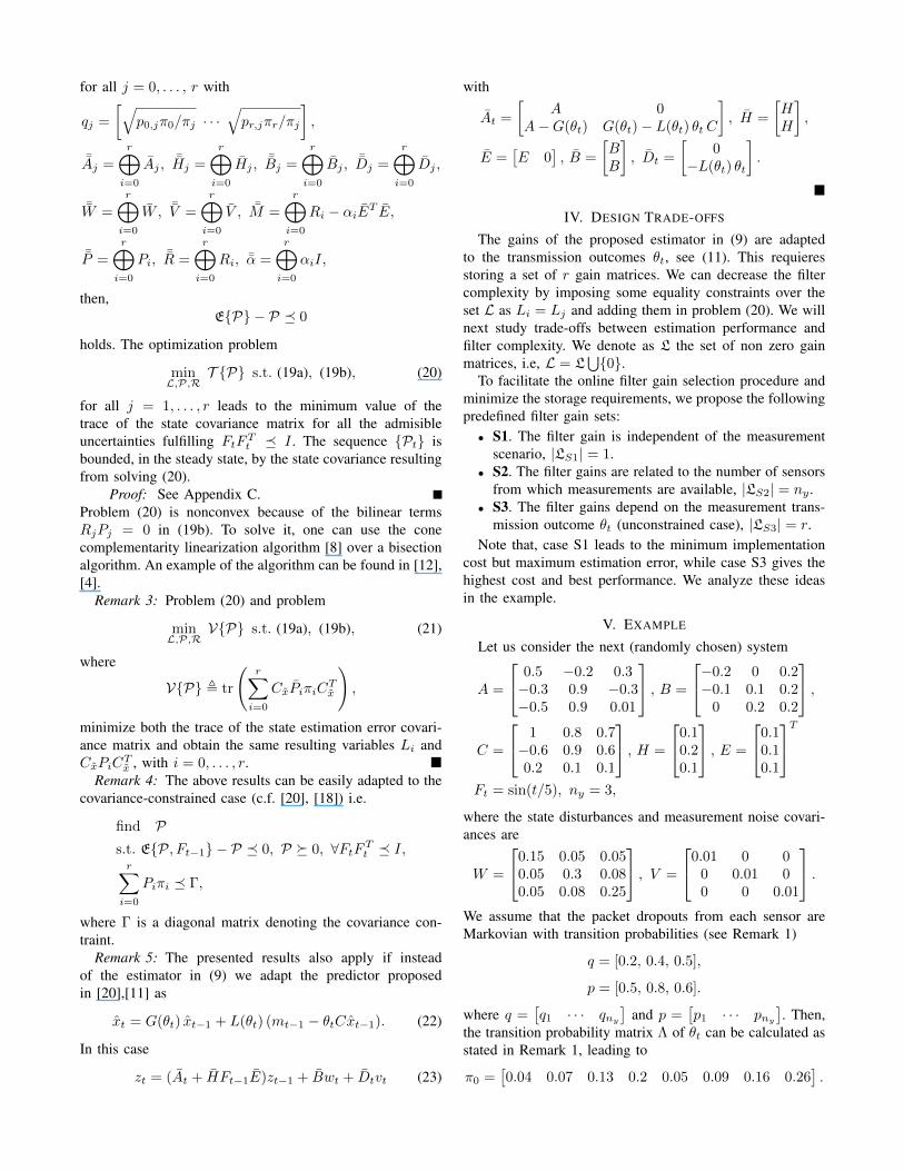
Fig. 2. Evolution of the actual trace of the state estimation error covariancefor cases S1, S2 and S3.

approaches. Both the initial state and the initial state esti-mation have been random initialized. In all the cases, in thesteady state (when t → ∞), the actual trace is above of itsbound obtained from (20), i.e. under V{P}. Case S3 leadsto the best estimation performance at the cost of using themost filter gains, while case C1 has the worst behavior butwith only one filter gain.

VI. CONCLUSIONS

In this paper, we have studied the state estimation prob-lem for a discrete-time linear system with time-varyingbounded uncertainty in the state matrix. The system outputmeasurements arrive to an estimation unit trough a net-work with different dropouts characteristics for each sensortransmission. We have modeled the measurement outcometransmission at each time instant with a finite Markovianprocess. Using this process, we have designed a jump stateestimator that minimizes the upperbound of the trace of thesteady state estimation error covariance for all the posibleuncertainties. Our design procedure allows to reduce the es-timator complexity at the cost of deteriorating the estimationperformances.

Further research directions may include extensions of thecurrent results to delayed measurements and uncertain outputmatrices.

VII. ACKNOWLEDGMENTS

This work has been supported by MICINN project numberDPI2011-27845-C02-0, and grant PREDOC/2011/37 fromUniversitat Jaume I.

REFERENCES

[1] P. Bremaud. Markov Chains. Springer, New York, 1999.[2] B. Chen, L. Yu, and W-A Zhang. Robust Kalman filtering for

uncertain state delay systems with random observation delays andmissing measurements. IET Control Theory Appl., 5(17):1945–1954,2011.

[3] J. Chen, K. H. Johansson, S. Olariu, I. Ch. Paschalidis, and I. Stoj-menovic. Guest editorial special issue on wireless sensor and actuatornetworks. IEEE Trans. Autom. Control, 56(10):2244–2246, 2011.

[4] H. Dong, Z. Wang, D. W. C. Ho, and H. Gao. Variance-constrainedH∞ filtering for a class of nonlinear time-varying systems withmultiple missing measurements: the finite-horizon case. IEEE Trans.Signal Process., 58(5):2534–2543, 2010.

[5] H. Dong, Z. Wang, D. W. C. Ho, and H. Gao. Robust H∞ filtering forMarkovian jump systems with randomly occurring nonlinearities andsensor saturation: the finite-horizon case. IEEE Trans. Signal Process.,59(7):3048–3057, 2011.

[6] L. El Ghaoui, F. Oustry, and M. AitRami. A cone complementaritylinearization algorithm for static output-feedback and related problems.IEEE Trans. Autom. Control, 42(8):1171–1176, 1997.

[7] R. A. Gupta and M.-Y. Chow. Networked control system: Overviewand research trends. IEEE Trans. Ind. Electron., 57(7):2527–2535,2010.

[8] J. P. Hespanha, P. Naghshtabrizi, and Y. Xu. A survey of recent resultsin networked control systems. Proceedings of the IEEE, 95(1):138–162, 2007.

[9] M. S. Mahmoud, P. Shi, and A. Ismail. Robust Kalman filtering fordiscrete-time Markovian jump systems with parameter uncertainty. J.Comput. Appl. Math, 169(1):53–69, 2004.

[10] I. Penarrocha, D. Dolz, and R. Sanchis. Inferential networked controlwith accessibility constraints in both the sensor and actuator channels.Int. J. Syst. Sci., 45(5):1180–1195, 2014.

[11] I. Penarrocha, R. Sanchis, and P. Albertos. Estimation in multisensornetworked systems with scarce measurements and time varying delays.Syst. Control. Lett., 61(4):555–562, 2012.

[12] L. Schenato. Optimal estimation in networked control systems subjectto random delay and packet drop. IEEE Trans. Autom. Control,53(5):1311–1317, 2008.

[13] B. Sinopoli, L. Schenato, M. Franceschetti, K. Poolla, M. I. Jordan,and S. S. Sastry. Kalman filtering with intermittent observations. IEEETrans. Autom. Control, 49(9):1453–1464, 2004.

[14] S. C. Smith and P. Seiler. Estimation with lossy measurements:jump estimators for jump systems. IEEE Trans. Automat. Contr.,48(12):2163–2171, 2003.

[15] B. Wang, G. Guo, and X. Gao. Variance-constrained robust estimationfor discrete-time systems with communication constraints. Math.Probl. Eng., 2014, 2014.

[16] B. Wang, G. Guo, and W. Yue. Variance-constrained robust estimationfor uncertain systems with multiple packet dropouts. Optim. ControlAppl. Methods, 34(1):53–68, 2013.

[17] Y. Wang, L. Xie, and C. E. de Souza. Robust control of a class ofuncertain nonlinear systems. Syst. Control Lett., 19(2):139–149, 1992.

[18] Z. Wang, D. W. C. Ho, and X. Liu. Variance-constrained filtering foruncertain stochastic systems with missing measurements. IEEE Trans.Automat. Contr., 48(7):1254–1258, 2003.

[19] Z. Wang, D. W. C. Ho, and X. Liu. Robust filtering under randomlyvarying sensor delay with variance constraints. IEEE Trans. CircuitsSyst. II, Exp. Briefs, 51(6):320–326, June 2004.

APPENDIX

A. Proof of Theorem 1

Equation (15) is obtained using the law of total probabil-ities. Considering the independency between xt−1, vt andwt−1, Pt,j = E{ztzTt |θt = ϑj} can be calculated as follows

r∑

i=0

Pr{θt−1 = ϑi|θt = ϑj}E{ztzTt |θt−1 = ϑi, θt = ϑj} =

r∑

i=0

pi,jπi

πj(Aj + HjFt−1E)︸ ︷︷ ︸

⋆

E{xt−1xTt−1|θt−1 = ϑi}⋆T

+r∑

i=0

pi,jπi

πj

(BjE{wt−1w

Tt−1}BT

j + DjE{vtvTt }DTj

),

which leads to (16) after using Bayes’ theorem, i.e.Pr{θt−1 = ϑi|θt = ϑj} = Pr{θt = ϑj |θt−1 =ϑi}Pr{θt−1 = ϑi}/Pr{θt = ϑj}.

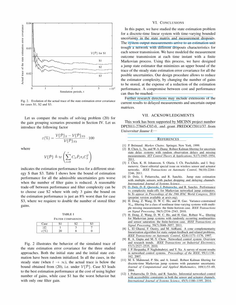
Fig. 2. Evolution of the actual trace of the state estimation error covariancefor cases S1, S2 and S3.

Let us compare the results of solving problem (20) forthe gain grouping scenarios presented in Section IV. Let usintroduce the following factor

ε(%) =V{P}S − V{P}S3

V{P}S3· 100

where

V{P} , tr

(r∑

i=0

CxPiπiCTx

)

indicates the estimation performance loss for a different strat-egy S than S3. Table I shows how the bound of estimationperformance for all the admissible uncertainties gets worsewhen the number of filter gains is reduced. A reasonabletrade-off between performance and filter complexity can beto choose case S2 where with only 3 gains the bound onthe estimation performance is just an 8% worst than for caseS3, where we requiere to double the number of stored filtergains.

TABLE IFILTER COMPARISON.

Case S1 S2 S3|L| 1 3 7ε(%) 20 8 0

Fig. 2 illustrates the behavior of the simulated trace ofthe state estimation error covariance for the three studiedapproaches. Both the initial state and the initial state esti-mation have been random initialized. In all the cases, in thesteady state (when t → ∞), the actual trace is below thebound obtained from (20), i.e. under V{P}. Case S3 leadsto the best estimation performance at the cost of using highernumber of gains, while case S1 has the worst behavior butwith only one filter gain.

VI. CONCLUSIONS

In this paper, we have studied the state estimation problemfor a discrete-time linear system with time-varying boundeduncertainty in the state matrix and measurement dropouts.The system output measurements arrive to an estimation unittrough a network with different dropouts characteristics foreach sensor transmission. We have modeled the measurementoutcome transmission at each time instant with a finiteMarkovian process. Using this process, we have designeda jump state estimator that minimizes an upper bound of thetrace of the steady state estimation error covariance for all theposible uncertainties. Our design procedure allows to reducethe estimator complexity, by changing the number of gainsto be stored, at the expense of a reduction of the estimationperformance. A compromise between cost and performancecan thus be reached.

Further research directions may include extensions of thecurrent results to delayed measurements and uncertain outputmatrices.

VII. ACKNOWLEDGMENTS

This work has been supported by MICINN project numberDPI2011-27845-C02-0, and grant PREDOC/2011/37 fromUniversitat Jaume I.

REFERENCES

[1] P. Bremaud. Markov Chains. Springer, New York, 1999.[2] B. Chen, L. Yu, and W-A Zhang. Robust Kalman filtering for uncertain

state delay systems with random observation delays and missingmeasurements. IET Control Theory & Applications, 5(17):1945–1954,2011.

[3] J. Chen, K. H. Johansson, S. Olariu, I. Ch. Paschalidis, and I. Stoj-menovic. Guest editorial special issue on wireless sensor and actuatornetworks. IEEE Transactions on Automatic Control, 56(10):2244–2246, 2011.

[4] D. Dolz, I. Penarrocha, and R. Sanchis. Jump state estimationwith multiple sensors with packet dropping and delaying channels.International Journal of Systems Science.

[5] D. Dolz, D. E. Quevedo, I. Penarrocha, and R. Sanchis. Performancevs complexity trade-offs for Markovian networked jump estimators.In To appear in Proceedings of the 19th IFAC World Congress, 2014(preprint version available at arxiv.org).

[6] H. Dong, Z. Wang, D. W. C. Ho, and H. Gao. Variance-constrainedH∞ filtering for a class of nonlinear time-varying systems with multi-ple missing measurements: the finite-horizon case. IEEE Transactionson Signal Processing, 58(5):2534–2543, 2010.

[7] H. Dong, Z. Wang, D. W. C. Ho, and H. Gao. Robust H∞ filteringfor Markovian jump systems with randomly occurring nonlinearitiesand sensor saturation: the finite-horizon case. IEEE Transactions onSignal Processing, 59(7):3048–3057, 2011.

[8] L. El Ghaoui, F. Oustry, and M. AitRami. A cone complementaritylinearization algorithm for static output-feedback and related problems.IEEE Transactions on Automatic Control, 42(8):1171–1176, 1997.

[9] R. A. Gupta and M.-Y. Chow. Networked control system: Overviewand research trends. IEEE Transactions on Industrial Electronics,57(7):2527–2535, 2010.

[10] J. P. Hespanha, P. Naghshtabrizi, and Y. Xu. A survey of recent resultsin networked control systems. Proceedings of the IEEE, 95(1):138–162, 2007.

[11] M. S. Mahmoud, P. Shi, and A. Ismail. Robust Kalman filtering fordiscrete-time Markovian jump systems with parameter uncertainty.Journal of Computational and Applied Mathematics, 169(1):53–69,2004.

[12] I. Penarrocha, D. Dolz, and R. Sanchis. Inferential networked controlwith accessibility constraints in both the sensor and actuator channels.International Journal of Systems Science, 45(5):1180–1195, 2014.

[13] I. Penarrocha, R. Sanchis, and P. Albertos. Estimation in multisensornetworked systems with scarce measurements and time varying delays.Systems & Control Letters, 61(4):555–562, 2012.

[14] L. Schenato. Optimal estimation in networked control systems subjectto random delay and packet drop. IEEE Transactions on AutomaticControl, 53(5):1311–1317, 2008.

[15] B. Sinopoli, L. Schenato, M. Franceschetti, K. Poolla, M. I. Jordan,and S. S. Sastry. Kalman filtering with intermittent observations. IEEETransactions on Automatic Control, 49(9):1453–1464, 2004.

[16] S. C. Smith and P. Seiler. Estimation with lossy measurements: jumpestimators for jump systems. IEEE Transactions on Automatic Control,48(12):2163–2171, 2003.

[17] B. Wang, G. Guo, and X. Gao. Variance-constrained robust estimationfor discrete-time systems with communication constraints. Mathemat-ical Problems in Engineering, 2014.

[18] B. Wang, G. Guo, and W. Yue. Variance-constrained robust estimationfor uncertain systems with multiple packet dropouts. Optimal ControlApplications and Methods, 34(1):53–68, 2013.

[19] Y. Wang, L. Xie, and C. E. de Souza. Robust control of a class ofuncertain nonlinear systems. Systems & Control Letters, 19(2):139–149, 1992.

[20] Z. Wang, D. W. C. Ho, and X. Liu. Variance-constrained filteringfor uncertain stochastic systems with missing measurements. IEEETransactions on Automatic Control, 48(7):1254–1258, 2003.

[21] Z. Wang, D. W. C. Ho, and X. Liu. Robust filtering under randomlyvarying sensor delay with variance constraints. IEEE Transactions onCircuits and Systems II: Express Briefs, 51(6):320–326, 2004.

APPENDIX

A. Proof of Theorem 1

Equation (15) is obtained using the law of total probabil-ities. Considering the independency between xt−1, vt andwt−1, Pt,j = E{ztzTt |θt = ϑj} can be calculated as follows

r∑

i=0

Pr{θt−1 = ϑi|θt = ϑj}E{ztzTt |θt−1 = ϑi, θt = ϑj} =

=

r∑

i=0

pi,jπiπj

(Aj + HjFt−1E)︸ ︷︷ ︸?

E{xt−1xTt−1|θt−1 = ϑi}?T

+

r∑

i=0

pi,jπiπj

(BjE{wt−1w

Tt−1}BT

j + DjE{vtvTt }DTj

),

which leads to (16) after using Bayes’ theorem, i.e.

Pr{θt−1 = ϑi|θt = ϑj}Pr{θt = ϑj} =

= Pr{θt = ϑj |θt−1 = ϑi}Pr{θt−1 = ϑi}B. Proof of Theorem 2

First, let us show the evolution of sequence {Gt} withinitial value

G0 � Pwhere Gt , (Gt,0, . . . , Gt,r). Le us introduce the variableZt , (Zt,0, . . . , Zt,r) with Zt,i = Gt,i−Pi. Then subtractingthe first inequality on (17b) from G1 = E{G0, F0} we get

Z1,j �r∑

i=0

pi,jπiπj

(Aj + HjF0E)Z0,i(Aj + HjF0E)T

(25)

for all j = 0, . . . , r. The only possible option for (25) tohold, given that G0 � P and (17b), is Z1,j � 0 that meansG1,j � P1,j and therefore G1 � P . By induction, we getthat the sequence {Gt} is bounded by P , i.e.,

Gt � P

for any t and any uncertainty fulfilling FtFTt � I when

G0 � P .Second, let us study the evolution of a sequence {Qt}

with initial valueQ0 � P

where Qt , (Qt,0, . . . , Qt,r). As P gives the minimumT {P} that fulfills (17b), for any Q0 � P we have thatQ1 = E{Q0, F0} � Q0. Then, for any Qt−1 � P , we have

Qt = E{Qt−1, Ft−1} � Qt−1.

Therefore, the sequence {Qt} is nonincreasing and whent → ∞ we have that Qt � P for any uncertainty fulfillingFtF

Tt � I .

Finally, let us prove that for any P0 � 0 the iterationPt = E{Pt−1, Ft−1} is bounded by P for any FtF

Tt � I .

Since P0 can be bounded by

0 � P0 � Q0

(with Q0 = P0 + P), we derive by induction that at a giveninstant t1 0 � Pt1 � Qt1 � P . Defining Gt1 as Qt1 � Gt1 �P , then

0 � Pt1 � Gt1 .Therefore as, sequences Gt is always bounded by P , then thesequence {Pt} is also bounded by P and the boundednessis demonstrated.

C. Proof of Theorem 3

If constraint (19b) holds it means that Ri = P−1i for alli = 0, . . . , r. Applying Schur’s complements over Pj in (19a)leads to

Ψj − Pj � 0, ∀j = 0, . . . , r (26)

with

Ψj =

r∑

i=0

pi,jπiπj

(Aj(P

−1i − αiE

T E)ATj + α−1i HjH

Tj

)

+

r∑

i=0

pi,jπiπj

(BjWBjT +DjV D

Tj

).

Note that A must be Schur’s stable for (26) to hold. ApplyingLemma 1 on the above equation, we get

Ej(P, Ft−1)− Pj � Ψj − Pj � 0,

∀j = 0, . . . , r, ∀FtFTt � I.

Therefore (19) guarantees

E{P, Ft−1} − P � 0

for all the admisible uncertainties fulfilling the condition onTheorem 2 that assures the boundedness of the sequence{Pt}.