A Hybrid Particle Swarm Optimization Algorithm for Clustering Analysis

14 Int. J. Bio-Inspired Computation, Vol. 1, Nos. 1/2, 2009

Copyright © 2009 Inderscience Enterprises Ltd.

Hybrid particle swarm optimization algorithm with fine tuning operators

G. Ramana Murthy*, M. Senthil Arumugam and C.K. Loo Faculty of Engineering and Technology, Multimedia University, 75450 Malacca, Malaysia E-mail: [email protected] E-mail: [email protected] E-mail: [email protected] *Corresponding author

Abstract: This paper introduces a new approach called hybrid particle swarm optimization like algorithm (hybrid PSO) with fine tuning operators to solve optimisation problems. This method combines the merits of the parameter-free PSO (pf-PSO) and the extrapolated particle swarm optimization like algorithm (ePSO). In order to accelerate the PSO algorithms to obtain the global optimal solution, three fine tuning operators, namely mutation, cross-over and root mean square variants are introduced. The effectiveness of the fine tuning elements with various PSO algorithms is tested through three benchmark functions along with a few recently developed state-of-the-art methods and the results are compared with those obtained without the fine tuning elements. From several comparative analyses, it is clearly seen that the performance of all the three PSO algorithms (pf-PSO, ePSO, and hybrid PSO) is considerably improved with various fine tuning operators and sometimes more competitive than the recently developed PSO algorithms.

Keywords: particle swarm optimization; PSO; benchmark problems; inertia weight; acceleration coefficient; mutation operators; cross-over operators; RMS variants.

Reference to this paper should be made as follows: Ramana Murthy, G, Senthil Arumugam, M. and Loo, C.K. (2009) ‘Hybrid particle swarm optimization algorithm with fine tuning operators’, Int. J. Bio-Inspired Computation, Vol. 1, Nos. 1/2, pp.14–31.

Biographical notes: Gajula Ramana Murthy is currently working as Lecturer in the Faculty of Engineering and Technology at Multimedia University, Malaysia. He obtained his BTech degree in 1991 from Nagarjuna University, AP, India, and MTech in 1993 from G.B. Pant Univ. of Agr. and Tech., India. His research focuses on evolutionary computation in embedded systems and memory optimisation in distributed computing.

M. Senthil Arumugam is currently working as Lecturer in the Faculty of Engineering and Technology at Multimedia University, Malaysia. He obtained his BE in 1994 from Madras University, India and MS (Eng.) in 1998 from BITS, Pilani, India. He received his PhD in Engineering from Multimedia University in 2008. He has been in the teaching field since 1996. His field of research work is on evolutionary computation in control system and embedded systems. He is currently a Reviewer for Applied Soft Computing Journal and few other international journals. He is invited to be a Guest Editor for Scientific Publications.

Chu Kiong Loo obtained his BE in Mechanical Engineering from University of Malaya (UM), Malaysia in 1996 and PhD from University of Science, Malaysia in 2004. He has been an Academic Staff of Multimedia University since 2001 and currently holds the post of Senior Lecturer. His research interest is in humanoid, ubiquitous robotics, soft-computing and quantum bio-inspired visual perception.

1 Introduction

The particle swarm optimization (PSO) algorithm is a parallel evolutionary computation technique introduced by Kennedy and Eberhart (1995) based on the social behaviour metaphor. It is a population-based optimisation technique, as an alternative tool to genetic algorithms (GA) and has gained lots of attention in various optimal control system

applications. PSO, a stochastic search technique with reduced memory requirement, is computationally effective and is easier to implement compared to other evolutionary algorithms (EAs). Also, PSO does not follow the survival of the fittest which is the principle of other EAs. PSO, when compared to other EAs, has very fast converging characteristics; however, it has a slow fine-tuning ability of

Hybrid particle swarm optimization algorithm with fine tuning operators 15

the solution. PSO has more global searching ability at the beginning of the run and local search near the end of the run (Kennedy and Eberhart, 1995). Therefore, while solving problems with more local optima, there are more possibilities for the PSO to explore local optima at the end of the run. Several researches were carried out so far to analyse the performance of the PSO with different settings, e.g., neighbourhood settings (Angeline, 1998; Eberhart and Kennedy, 1995; Ratnaweera et al., 2004; Senthil Arumugam et al., 2007b).

Angeline (1998, 1999) introduced a new version of the PSO that incorporates the concept of selection for PSO algorithm. According to Angeline (1998), the current PSO algorithm is in poor form of selecting the particles by considering the personal best position as additional population members. In the gbest PSO model, a particle is restricted to access only the ‘gbest’ particles and hence restricted 50% of the interaction with the other particles. The purpose of selection in any EAs is to focus the effort of the algorithm on a specific region of the search space. Following the work of Angeline (1999), various mutation operators for a single stage hybrid manufacturing system via conventional PSO (cPSO) and global-local best PSO (GLBest PSO) are incorporated (Senthil Arumugam et al., 2007b). Later, Lovbjerg et al. (2001) chose to investigate the effect of cross-over operator with PSO. Arithmetic cross-over operation was carried out between two randomly selected particles producing two new children replacing their parents. This process is repeated for a number of particles with probability Pc. Thus, the arithmetic cross-over of the positions yields two new positions at random locations. The velocity crossover normalises the length of the sum of the two parent’s velocities, so that only the direction and not the magnitude are affected. The results presented in Lovbjerg et al., (2001) show that the cross-over slows down the rate of convergence on unimodal functions but for the functions with many local minima, crossover takes the lead. Lovbjerg et al. (2001) applied cross-over only for gbest model PSO and no comparison with lbest model.

In this paper, three different fine tuning operators namely, mutation, cross-over and RMS variants are incorporated with pf-PSO, ePSO and hybrid PSO methods and their influences in the improvement of the algorithms are examined for a few benchmark problems. The results are compared with one other with and with out the fine tuning variants and also with those obtained via cPSO [PSO with time varying inertia weight (TVIW)] and GLBest PSO (Senthil Arumugam et al., 2007b). To further strengthen the comparison, the proposed methods are also compared with a few recently developed state-of-the-art papers (Mendes et al., 2004; Parsopoulos and Vrahatis, 2004; Peram et al., 2003; Van Den Bergh and Engelbrecht, 2004).

This paper is organised as follows: in Section 2, a brief review of cPSO and GLBest PSO algorithms is presented; in Section 3, the proposed hybrid PSO algorithm is described along with pf-PSO and ePSO; the design of the fine tuning elements such as mutation, cross-over and RMS

variants is discussed in Section 4; in Sections 5 and 6, the performance of the cPSO, GLBest PSO, pf-PSO, ePSO and hybrid PSO algorithms with and without the fine tuning elements are analysed and compared for three difficult benchmark problems; in Section 7, the performance of the proposed methods with and without FTE is compared with a few state-of-the-art methods and finally the conclusions are given in Section 8.

2 Review of cPSO and GLBest PSO algorithms

The cPSO algorithm considered in this paper comprises standard PSO algorithm (Eberhart and Kennedy, 1995; Eberhart et al., 1996; Kennedy and Eberhart, 1995; Shi and Eberhart, 1998b) with TVIW and time varying acceleration coefficient (TVAC). The velocity and position equation for this method is given in equations (1) and (2)

( ) ( ) ( )( )

1 1

2 2

1 ( ) ( )

( ) ( )i i i i

i i

v t w v t c r t pbest x t

c r t gbest x t

= ⋅ − + × × −

+ × × − (1)

( ) ( ) ( )1i i ix t x t v t= − + (2)

The TVIW which is developed (Eberhart et al., 1996; Shi and Eberhart, 1998a) is given in equation (3).

1 2 2max TVIW ( )

maxiter iterw w w w

iter−⎛ ⎞= = − +⎜ ⎟

⎝ ⎠ (3)

where w1 and w2 are the initial and final values of the inertia weight respectively, iter is the current iteration number and maxiter is the maximum number of allowable iterations.

Ratnaweera et al. (2004) introduced a TVAC which is given in equations (4) and (5). In this method, the TVAC reduces the ‘cognitive’ component and increases the ‘social’ component of acceleration coefficient, c1 and c2 with time.

1 1 1 1max( )

maxi f fiter iterc c c c

iter−⎛ ⎞= − +⎜ ⎟

⎝ ⎠ (4)

2 2 2 2max( )

maxi f fiter iterc c c c

iter−⎛ ⎞= − +⎜ ⎟

⎝ ⎠ (5)

where c1i and c2i are the initial values of the acceleration coefficients c1 and c2; c1f and c2f are the final values of the acceleration coefficients c1 and c2 respectively.

The GLBest PSO method (Senthil Arumugam et al., 2005, 2007b) in which, the inertia weight and acceleration coefficients are neither set to a constant value nor set as a linearly decreasing time varying function. Instead, they are defined as a function of local best (pbest) and global best (gbest) values of the particles in each generation. The GLBest inertia weight (GLBest IW) and GLBest acceleration coefficients (GLBest AC) are given in equations (6) and (7).

1.1( )

ii

i average

gbestGLBestIW w

pbest⎛ ⎞

= = −⎜ ⎟⎜ ⎟⎝ ⎠

(6)

16 G. Ramana Murthy et al.

1( )

i

i

gbestGLBestAC C

pbest⎛ ⎞

= = +⎜ ⎟⎝ ⎠

(7)

The velocity equation for GLBest PSO is also modified as given in equation (8) while the position equation remains same as in the cPSO method.

( ) ( ) ( )11 ( 2 )i i i iv t w v t c r pbest gbest x t= ⋅ − + ⋅ + − (8)

3 Novel approaches to PSO algorithm

Recently, Senthil Arumugam et al. (2007a, 2007b) introduced two new PSO like algorithms namely, the parameter-free PSO (pf-PSO) and the particle swarm optimization like algorithm via extrapolation (ePSO).

3.1 Parameter-free PSO algorithm (pf-PSO)

In pf-PSO algorithm, the position of each particle is updated directly with the local best and global best particle positions and it does not have any velocity equation. In addition, this method does not require any parameters such as inertia weight and the acceleration coefficient. Other than these differences, the pf-PSO method is conceptually similar to the functional behaviour of cPSO. The updated position of each particle is calculated from equation (9).

1 2( ) 1 * * * *( 1) ( 1)i i

i i

gbest gbestx t Rnd gbest Rnd pbestx t x t

⎛ ⎞ ⎛ ⎞= − +⎜ ⎟ ⎜ ⎟− −⎝ ⎠ ⎝ ⎠

(9)

where gbest is the global best value obtained so far until that level of search whereas pbesti is the local best value obtained in that particular population. The random functions (Rnd1 and Rnd2) ensure the stochastic behaviour of the algorithm. The values of Rnd1 and Rnd2 are used to maintain the diversity of the population and they are uniformly distributed in the range of zero to one.

3.2 Extrapolated PSO algorithm (ePSO)

In the ePSO algorithm, the current particle position and the global best particle position are involved in the extrapolation operation. The current particle position of each particle is updated by extrapolating the global best particle position in order to refine the search towards the global optimum value. This ePSO algorithm also includes two extrapolation coefficients (e1 and e2) which are varying from 0.999 to 0.36. A random function (Rnd1) is also included to incorporate the stochastic behaviour into the algorithm’s search to find the optimal solution. The updated position equation for each particle is given in equation (10).

1 1 1

2

( ) [ ] [ * * ] [ *( ( 1))*exp( *(( ( ) ( ( 1)))/ ( )))]

i i

i

x t gbest e Rnd gbest e gbest x te f gbest f x t f gbest= + + − −

− − (10)

where

e1 and e2 = exp (–current generation/max. no. of generation).

f(gbest) is the fitness value at gbest position

f (xi(t)) is the current particle’s fitness value.

3.3 Hybrid PSO algorithm

To incorporate the merits of both the pf-PSO and ePSO methods together into a single method, a hybrid combination of both these methods (hybrid PSO) is proposed in this paper. Various hybrid combinations of pf-PSO and ePSO methods are considered and tested with the standard benchmark problems. From the empirical study of the hybrid combinations, a best hybrid combination of pf-PSO and ePSO method is identified. In the hybrid PSO method, ePSO method is simulated for the first 50% of the total generations and pf-PSO method is implemented in the remaining generations. The ePSO method directs the hybrid PSO method to move closer to the exact optimal solution and then pf-PSO method triggers the hybrid PSO method to reach the optimal solution with a faster convergence rate. Hence, the hybrid PSO method first identifies a near optimal fitness solution and then produces a better solution with a faster convergence rate.

4 Fine tuning operators

Three fine tuning operators namely, mutation, crossover and RMS variants as discussed in Senthil Arumugam et al. (2007b) are incorporated with the three different versions of PSO algorithms, pf-PSO (Senthil Arumugam et al., 2007c), ePSO (Senthil Arumugam et al., 2007a) and hybrid PSO methods to improve their performances. The hybrid PSO method comprises of a hybrid combination of both pf-PSO and ePSO methods (Senthil Arumugam et al., 2007b). These three fine tuning operators were incorporated with cPSO and GLBest PSO methods. In this paper, the effectiveness of these operators is once again tested with the other three PSO algorithms and compared with the results obtained for cPSO and GLBest PSO algorithms.

4.1 Mutation operators

Mutation plays an important role in the development of genetic algorithm (Gen and Cheng, 1997). It is designed for fine-tuning capabilities aimed at achieving high precision. Hence, PSO algorithm with mutation has the potential to reach a better solution. The three mutation operators considered for fine-tuning the PSO performance are listed in Table 1.

Hybrid particle swarm optimization algorithm with fine tuning operators 17

Table 1 Mutation operators

Mutation type Mutation equation

1 No mutation – 2 Single dimension

mutation (SDM) Mutation variant 1 (M1)

1 2

1 2 1

0.010.01

i

i

X Xr XorX Xr Xor+

= + ×

= + ×

3 Two dimension mutation (TDM) Mutation variant 2 (M2)

1 2 3

1 2 1 3

2 3 1 2

0.01 0.010.01 0.010.01 0.01

i

i

i

X Xr Xor XorX Xr Xor XorX Xr Xor Xor

+

+

= + × + ×

= + × + ×

= + × + ×

4 Differential mutation (DM) Mutation variant 3 (M3)

3 1 20.01 ( )iX Xr Xor Xor= + × −

4.2 Cross-over variants

In many papers on evolutionary computation, crossover is the main genetic operator (Michalewicz, 1992) and consists of swapping chromosome parts between individuals. Crossover is not performed on every pair of individuals, its frequency being controlled by a crossover probability (Pc). There are several crossover methods available, among them three cross-over operators namely, arithmetic crossover (AMXO), average convex crossover (ACXO) and root probability cross-over (RPXO) (Gen and Cheng, 1997; Michalewicz, 1992) are considered for fine tuning the performance of various PSO algorithms. The mathematical representation of these three cross-over methods is listed in Table 2.

4.3 Root-mean square (RMS) variants

The RMS variants are used to fine tune the performance of various PSO algorithms in order to obtain a more precise solution and also to improve the convergence rate. Here, three such RMS variants are considered and each of these three RMS variants differs from one another by the number of samples considered in the RMS equation and presented in Table 3.

In the first variant, two chromosomes (say, parents) are involved and a new chromosome (child) is developed and hence named as the 2-D RMS variant.

In the second variant, three chromosomes are involved, one from the current particle and the other two are selected randomly from the other remaining particles, to create a new population.

The third variant is a hybrid RMS variant in which a group of three chromosomes is considered and from the combinations of these three and randomly selected particles, three new chromosomes are developed.

The notations such as Xr1, Xr2, Xr3 represent randomly chosen values within a particle itself whereas Xor1, Xor2, Xor3 are the random values from any other two particles which are chosen for interaction. The randomly selected values Xr1, Xr2, Xr3 of the current particle are modified by the RMS variants.

Table 2 Cross-over operators

Cross-over Mathematical representation

1 No cross-over – 2 Arithmetic

cross-over (AMXO) Crossover variant 1 (C1)

( )( ) 1

1

x x y

x x y

λ λ

λ λ

′ = + −

′′ = − +

λ = [0 1]

3 Average convex cross-over (ACXO)Crossover variant 2 (C2)

( )( )

1

1

x x y

x x y

λ λ

λ λ

′ = + −

′′ = − +

where λ = 0.5

4 Root probability cross-over (RPXO)Crossover variant 3 (C3)

0.5 0.5( ) (1 )x x yλ λ′ = + − λ = [0 1]

Table 3 RMS variants

RMS variants Mathematical representation

1 No variants – 2 Two

dimensional RMS variant [RMS variant 1 (R1)]

2 21 2

3 2Xr XorXr +

=

3 Three dimensional RMS variant [RMS variant 2 (R2)]

2 2 21 2 3

3 3Xr Xor XorXr + +

=

4 Hybrid RMS variant [RMS variant 3 (R3)]

2 2 2 22 3 3 1

1 2

2 21 2

3

2 2

2

Xr Xor Xr XorXr Xr

Xr XorXr

+ += =

+=

5 Testing with benchmark problems

In order to validate the effectiveness of the fine tuning elements in improving the performance of the PSO algorithms, three difficult benchmark functions namely, Rosenbrock, Griewank and Schwefel functions are considered (Senthil Arumugam et al., 2007b; Van Den Bergh and Engelbrecht, 2004). The details about these three benchmark problems are given in the Appendix. All the five PSO algorithms (cPSO, GLBestPSO, pf-PSO, ePSO and hybrid PSO) are simulated with nine fine tuning elements comprising of three mutation operators (M1, M2 and M3), three cross-over operators (C1, C2 and C3) and three RMS variants (R1, R2 and R3) individually. Method A refers to the PSO. The simulation results are recorded for all the 500 runs individually. The simulated results for the PSO algorithms with the fine tuning elements are compared with those obtained without any fine tuning.

18 G. Ramana Murthy et al.

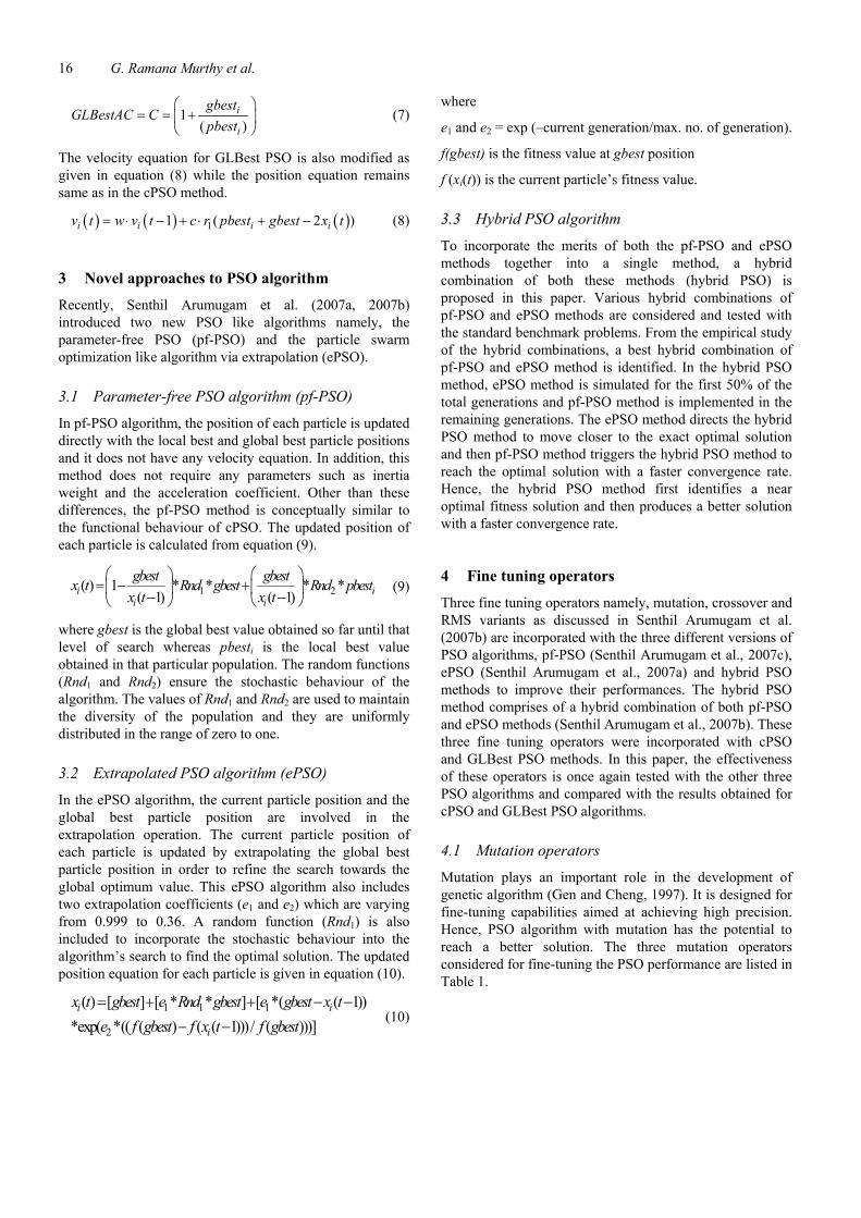
Table 4(a) cPSO algorithm with the fine tuning elements for solving the Rosenbrock function

cPSO Mean Max Min Median SD CV Mean gen

A 56.7933 158.611 3.9888 65.3748 38.2235 0.673 2000 M1 20.0486 28.7464 0.0121 25.4271 10.8234 0.5399 2000 M2 31.8648 108.3346 4.1811 26.0256 23.7756 0.7461 2000 M3 20.8553 26.1191 0.0001 25.4883 9.8775 0.4736 1633.5 C1 29.8524 80.3919 5.3413 26.2226 23.8011 0.7973 703.65 C2 29.7482 77.3142 0.0003 47.8368 40.9902 1.3779 817.05 C3 19.9993 25.8442 0 25.1508 9.8951 0.4948 572.68 R1 0.0001 0.0001 0 0.0001 0 0.5525 485.52 R2 0.6379 3.9866 0 0.0001 1.4208 2.2272 401.86 R3 16.5495 79.7882 0.0001 5.1612 25.9464 1.5678 412.35

Table 4(b) GLBest PSO algorithm with the fine tuning elements for solving the Rosenbrock function

GLBest PSO Mean Max Min Median SD CV Mean gen

A 53.6233 158.009 3.9871 60.8588 35.8485 0.6685 2000 M1 18.5535 27.454 0.0006 23.9653 10.7075 0.5771 2000 M2 31.1135 82.8993 3.9879 24.3616 21.4078 0.6881 2000 M3 20.4762 24.6673 0.0001 24.0559 8.0076 0.3911 1528.29 C1 28.9427 79.9235 3.9922 24.3706 21.4174 0.74 562.93 C2 25.0032 76.8327 0.0003 24.3522 20.8578 0.8342 762.73 C3 16.5906 24.3635 0 23.804 8.8256 0.532 323.75 R1 0.0001 0.0001 0 0.0001 0 0.6259 287.88 R2 0.319 3.9866 0 0.0001 1.1038 3.4603 303.93 R3 15.2668 76.7372 0.0001 4.235 23.3219 1.5276 387.02

Table 4(c) pf-PSO algorithm with the fine tuning elements for solving the Rosenbrock function

pf-PSO Mean Max Min Median SD CV Mean gen

A 0.000055 0.000094 0.000009 0.000054 0.000027 0.497325 240 M1 0.000031 0.000092 0 0.000019 0.000031 1.004407 218.76 M2 0.000032 0.000096 0.000001 0.000023 0.000023 0.721401 223.08 M3 0.000032 0.000092 0.000001 0.000024 0.00003 0.955715 224.36 C1 0.000035 0.00011 0.000001 0.000026 0.000031 0.890734 211.76 C2 0.000034 0.000189 0 0.000022 0.00004 1.168424 211.64 C3 0.000034 0.000093 0.000001 0.000029 0.000026 0.779435 236.04 R1 0.000025 0.000073 0 0.000014 0.000025 0.993147 205.92 R2 0.000026 0.000079 0 0.000008 0.000029 1.11482 206.8 R3 0.000025 0.000091 0 0.000019 0.000029 1.129561 204.4

Hybrid particle swarm optimization algorithm with fine tuning operators 19

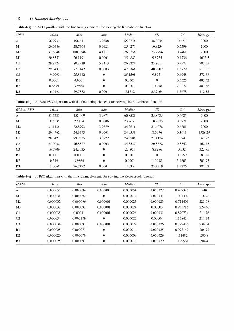
Table 4(d) ePSO algorithm with the fine tuning elements for solving the Rosenbrock function

ePSO Mean Max Min Median SD CV Mean gen

A 28.67408 28.93542 27.36302 28.90436 0.40724 0.0142 447.8 M1 28.53972 28.70499 27.78326 28.65204 0.2822 0.00989 379.04 M2 7.1834 27.93502 2.58618 5.95548 6.44774 0.89759 398.4 M3 14.05486 28.10727 0.17204 3.48901 13.62724 0.96958 413.42 C1 0.3858 1.6175 0.0129 0.21354 0.46522 1.20586 374 C2 27.4775 27.7061 27.24625 27.43655 0.17359 0.00632 604.28 C3 0.48105 1.96343 0.00472 0.24748 0.56306 1.17049 517.92 R1 0.72144 1.55965 0.0025 0.73855 0.40303 0.55864 364.2 R2 0.62226 1.99333 0.00203 0.49618 0.5642 0.90671 450.76 R3 0.33571 1.26164 0.00277 0.24615 0.3554 1.05866 321.6

Table 4(e) Hybrid PSO algorithm with the fine tuning elements for solving the Rosenbrock function

Hybrid PSO Mean Max Min Median SD CV Mean gen

A 5.34E–05 1.99E–04 6.60E–07 4.17E–05 4.55E–05 8.52E–01 399.24 M1 3.79E–05 9.90E–05 2.21E–07 2.69E–05 3.25E–05 8.58E–01 326.84 M2 4.72E–05 9.65E–05 3.72E–07 4.82E–05 3.41E–05 7.22E–01 276.96 M3 4.80E–05 1.61E–04 5.80E–08 4.38E–05 3.64E–05 7.57E–01 265.8 C1 4.37E–05 2.60E–04 2.10E–06 2.05E–05 5.46E–05 1.25E+00 269.84 C2 3.48E–05 9.94E–05 6.62E–07 3.05E–05 3.09E–05 8.88E–01 285.16 C3 4.54E–05 9.42E–05 5.65E–07 4.77E–05 3.19E–05 7.03E–01 275.6 R1 4.77E–05 1.73E–04 1.60E–06 4.92E–05 3.84E–05 8.06E–01 266.88 R2 3.45E–05 9.73E–05 4.04E–07 2.91E–05 2.85E–05 8.26E–01 351.72 R3 2.69E–05 8.99E–05 9.00E–07 1.29E–05 2.96E–05 1.10E+00 245.16

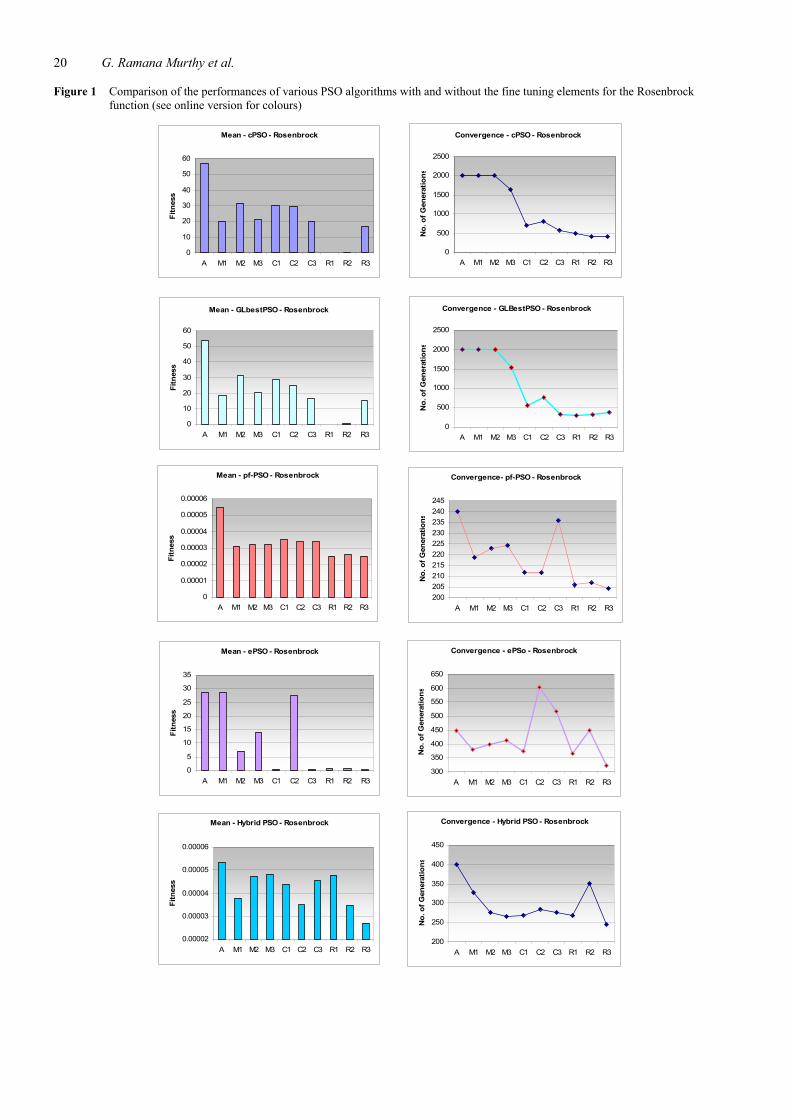
5.1 The Rosenbrock function

All the five PSO algorithms (cPSO, GLBest PSO, pf-PSO, ePSO, and hybrid PSO) are simulated with the nine fine tuning operators individually for solving the Rosenbrock function. The simulations are repeated for 500 times and various statistical analyses are carried out. The Performance of the PSO algorithms with the fine tuning elements is then compared with those obtained without the fine tuning elements and presented in Tables 4(a) to 4(e). The comparisons of the mean fitness values and the convergence rates between all the five PSO algorithms are plotted in Figure 1.

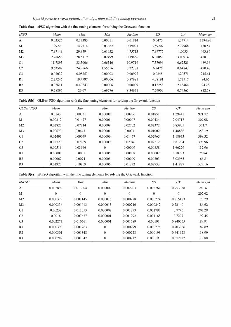
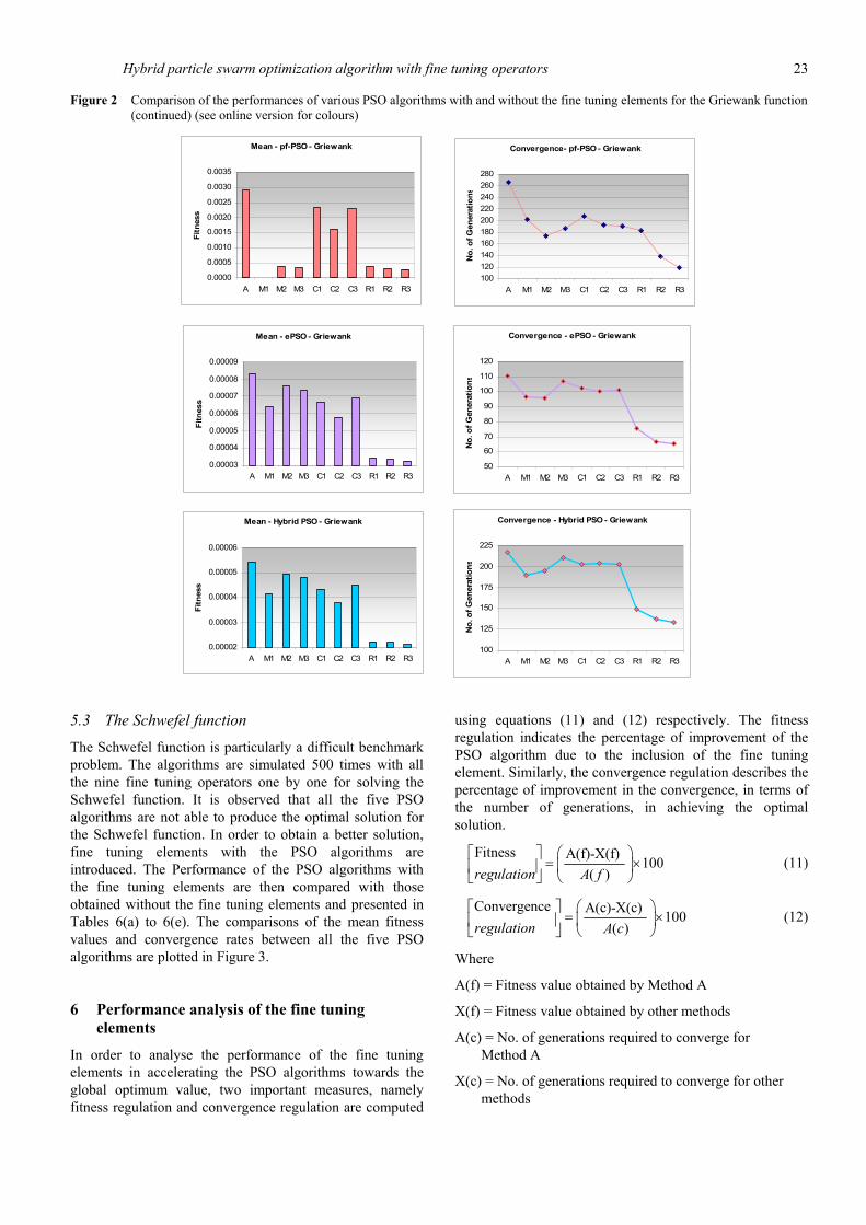
5.2 The Griewank function

All the five mentioned PSO algorithms are simulated 500 times with all the nine fine tuning operators one by one for solving the Griewank function. From the simulation, various statistical analyses are carried out. The performance of the PSO algorithms with the fine tuning elements is then compared with those obtained without the fine tuning elements and presented in Tables 5(a) to 5(e). The comparisons of the mean fitness values and the convergence rates between all the five PSO algorithms are plotted in Figure 2.

20 G. Ramana Murthy et al.

Figure 1 Comparison of the performances of various PSO algorithms with and without the fine tuning elements for the Rosenbrock function (see online version for colours)

Mean - cPSO - Rosenbrock

0

10

20

30

40

50

60

A M1 M2 M3 C1 C2 C3 R1 R2 R3

Fitn

ess

Convergence - cPSO - Rosenbrock

0

500

1000

1500

2000

2500

A M1 M2 M3 C1 C2 C3 R1 R2 R3

No.

of G

ener

atio

ns

Mean - GLbestPSO - Rosenbrock

0

10

20

30

40

50

60

A M1 M2 M3 C1 C2 C3 R1 R2 R3

Fitn

ess

Convergence - GLBestPSO - Rosenbrock

0

500

1000

1500

2000

2500

A M1 M2 M3 C1 C2 C3 R1 R2 R3

No.

of G

ener

atio

ns

Mean - pf-PSO - Rosenbrock

0

0.00001

0.00002

0.00003

0.00004

0.00005

0.00006

A M1 M2 M3 C1 C2 C3 R1 R2 R3

Fitn

ess

Convergence- pf-PSO - Rosenbrock

200205210215220225230235240245

A M1 M2 M3 C1 C2 C3 R1 R2 R3

No.

of G

ener

atio

ns

Mean - ePSO - Rosenbrock

0

5

10

15

20

25

30

35

A M1 M2 M3 C1 C2 C3 R1 R2 R3

Fitn

ess

Convergence - ePSo - Rosenbrock

300

350

400

450

500

550

600

650

A M1 M2 M3 C1 C2 C3 R1 R2 R3

No.

of G

ener

atio

ns

Mean - Hybrid PSO - Rosenbrock

0.00002

0.00003

0.00004

0.00005

0.00006

A M1 M2 M3 C1 C2 C3 R1 R2 R3

Fitn

ess

Convergence - Hybrid PSO - Rosenbrock

200

250

300

350

400

450

A M1 M2 M3 C1 C2 C3 R1 R2 R3

No.

of G

ener

atio

ns

Hybrid particle swarm optimization algorithm with fine tuning operators 21

Table 5(a) cPSO algorithm with the fine tuning elements for solving the Griewank function

cPSO Mean Max Min Median SD CV Mean gen

A 0.03526 0.17385 0.00011 0.01814 0.0475 1.34714 1394.86 M1 1.29226 14.7314 0.03682 0.19021 3.59207 2.77968 450.54 M2 7.97149 29.9594 0.61052 4.75713 7.99777 1.0033 463.86 M3 2.28656 28.5119 0.02499 0.19856 6.88059 3.00914 428.38 C1 11.7895 33.3006 0.66546 10.9719 7.37096 0.62521 489.16 C2 9.63502 24.9566 1.55556 8.22381 6.2476 0.64843 490.48 C3 0.02032 0.08253 0.00003 0.00997 0.0245 1.20571 215.61 R1 2.35246 19.4997 0.00006 0.87981 4.08191 1.73517 84.66 R2 0.05611 0.40243 0.00006 0.00009 0.12258 2.18464 94.28 R3 9.78896 26.07 0.69776 8.34671 7.29909 0.74565 812.58

Table 5(b) GLBest PSO algorithm with the fine tuning elements for solving the Griewank function

GLBest PSO Mean Max Min Median SD CV Mean gen

A 0.0143 0.08331 0.00008 0.00986 0.01851 1.29441 921.72 M1 0.00212 0.01477 0.00001 0.00007 0.00434 2.04717 309.08 M2 0.02827 0.07814 0.00009 0.02702 0.02372 0.83905 371.7 M3 0.00673 0.0443 0.00001 0.0001 0.01002 1.48886 353.19 C1 0.02493 0.09049 0.00006 0.01477 0.02965 1.18933 398.32 C2 0.02723 0.07089 0.00009 0.02946 0.02212 0.81234 396.96 C3 0.00516 0.03946 0 0.00009 0.00858 1.66279 132.96 R1 0.00008 0.0001 0.00005 0.00008 0.00002 0.18293 75.84 R2 0.00067 0.0074 0.00005 0.00009 0.00203 3.02985 66.8 R3 0.01927 0.10809 0.00006 0.01232 0.02733 1.41827 523.16

Table 5(c) pf-PSO algorithm with the fine tuning elements for solving the Griewank function

pf-PSO Mean Max Min Median SD CV Mean gen

A 0.002899 0.013004 0.000002 0.002203 0.002764 0.953358 266.6 M1 0 0 0 0 0 0 202.62 M2 0.000379 0.001145 0.000016 0.000278 0.000274 0.815183 173.29 M3 0.000336 0.001013 0.000015 0.000246 0.000242 0.721401 186.62 C1 0.00232 0.011053 0.000002 0.001873 0.001797 0.7746 207.28 C2 0.0016 0.007627 0.000001 0.001292 0.001168 0.7297 192.45 C3 0.002273 0.010561 0.000001 0.001789 0.00191 0.840065 189.91 R1 0.000393 0.001763 0 0.000299 0.000276 0.703066 182.89 R2 0.000301 0.001348 0 0.000228 0.000193 0.641628 138.99 R3 0.000287 0.001047 0 0.000212 0.000193 0.672822 118.88

22 G. Ramana Murthy et al.

Table 5(d) ePSO algorithm with the fine tuning elements for solving the Griewank function

ePSO Mean Max Min Median SD CV Mean gen

A 8.30E–05 1.00E–04 5.40E–05 8.70E–05 1.40E–05 1.73E–01 1.10E+02 M1 6.38E–05 7.64E–05 4.13E–05 6.68E–05 1.03E–05 1.62E–01 9.65E+01 M2 7.60E–05 9.09E–05 9.20E–06 7.95E–05 1.28E–05 1.68E–01 9.53E+01 M3 7.35E–05 8.80E–05 4.76E–05 7.69E–05 1.24E–05 1.68E–01 1.07E+02 C1 6.65E–05 8.46E–05 4.58E–05 7.40E–05 9.35E–06 1.41E–01 1.02E+02 C2 5.78E–05 7.35E–05 3.98E–05 6.43E–05 8.13E–06 1.41E–01 1.00E+02 C3 6.92E–05 8.59E–05 4.65E–05 7.51E–05 1.06E–05 1.54E–01 1.01E+02 R1 3.44E–05 4.12E–05 2.23E–05 3.60E–05 3.07E–06 8.93E–02 7.56E+01 R2 3.36E–05 4.02E–05 2.17E–05 3.52E–05 3.00E–06 8.93E–02 6.62E+01 R3 3.26E–05 3.91E–05 2.11E–05 3.42E–05 2.92E–06 8.93E–02 6.54E+01

Table 5(e) Hybrid PSO algorithm with the fine tuning elements for solving the Griewank function

Hybrid PSO Mean Max Min Median SD CV Mean gen

A 0.00005 0.0001 0.00002 0.00005 0.00002 0.39924 216.84 M1 0.00004 0.00008 0.00002 0.00004 0.00002 0.3731 189.95 M2 0.00005 0.00009 0.00002 0.00004 0.00002 0.3879 194.4 M3 0.00005 0.00009 0.00002 0.00004 0.00002 0.3879 210.33 C1 0.00004 0.00008 0.00002 0.00004 0.00001 0.3244 202.88 C2 0.00004 0.00007 0.00002 0.00003 0.00001 0.3244 203.83 C3 0.00005 0.00009 0.00002 0.00004 0.00002 0.3544 202.86 R1 0.00002 0.00004 0.00001 0.00002 0 0.2062 148.75 R2 0.00002 0.00004 0.00001 0.00002 0 0.2062 137.34 R3 0.00002 0.00004 0.00001 0.00002 0 0.2062 133.36

Figure 2 Comparison of the performances of various PSO algorithms with and without the fine tuning elements for the Griewank function (see online version for colours)

Mean - cPSO - Griewank

0

2

4

6

8

10

12

A M1 M2 M3 C1 C2 C3 R1 R2 R3

Fitn

ess

Convergence - cPSO - Griewank

0200400600800

1000120014001600

A M1 M2 M3 C1 C2 C3 R1 R2 R3

No.

of G

ener

atio

ns

Mean - GLbestPSO - Griewank

0.000

0.005

0.010

0.015

0.020

0.025

0.030

A M1 M2 M3 C1 C2 C3 R1 R2 R3

Fitn

ess

Convergence - GLBestPSO - Griewank

0

200

400

600

800

1000

A M1 M2 M3 C1 C2 C3 R1 R2 R3

No.

of G

ener

atio

ns

Hybrid particle swarm optimization algorithm with fine tuning operators 23

Figure 2 Comparison of the performances of various PSO algorithms with and without the fine tuning elements for the Griewank function (continued) (see online version for colours)

Mean - pf-PSO - Griewank

0.0000

0.0005

0.0010

0.0015

0.0020

0.0025

0.0030

0.0035

A M1 M2 M3 C1 C2 C3 R1 R2 R3

Fitn

ess

Convergence- pf-PSO - Griewank

100120140160180200220240260280

A M1 M2 M3 C1 C2 C3 R1 R2 R3

No.

of G

ener

atio

ns

Mean - ePSO - Griewank

0.00003

0.00004

0.00005

0.00006

0.00007

0.00008

0.00009

A M1 M2 M3 C1 C2 C3 R1 R2 R3

Fitn

ess

Convergence - ePSO - Griewank

50

60

70

80

90

100

110

120

A M1 M2 M3 C1 C2 C3 R1 R2 R3N

o. o

f Gen

erat

ions

Mean - Hybrid PSO - Griewank

0.00002

0.00003

0.00004

0.00005

0.00006

A M1 M2 M3 C1 C2 C3 R1 R2 R3

Fitn

ess

Convergence - Hybrid PSO - Griewank

100

125

150

175

200

225

A M1 M2 M3 C1 C2 C3 R1 R2 R3

No.

of G

ener

atio

ns

5.3 The Schwefel function

The Schwefel function is particularly a difficult benchmark problem. The algorithms are simulated 500 times with all the nine fine tuning operators one by one for solving the Schwefel function. It is observed that all the five PSO algorithms are not able to produce the optimal solution for the Schwefel function. In order to obtain a better solution, fine tuning elements with the PSO algorithms are introduced. The Performance of the PSO algorithms with the fine tuning elements are then compared with those obtained without the fine tuning elements and presented in Tables 6(a) to 6(e). The comparisons of the mean fitness values and convergence rates between all the five PSO algorithms are plotted in Figure 3.

6 Performance analysis of the fine tuning elements

In order to analyse the performance of the fine tuning elements in accelerating the PSO algorithms towards the global optimum value, two important measures, namely fitness regulation and convergence regulation are computed

using equations (11) and (12) respectively. The fitness regulation indicates the percentage of improvement of the PSO algorithm due to the inclusion of the fine tuning element. Similarly, the convergence regulation describes the percentage of improvement in the convergence, in terms of the number of generations, in achieving the optimal solution.

Fitness A(f)-X(f) 100 ( )regulation A f

⎛ ⎞⎡ ⎤= ×⎜ ⎟⎢ ⎥

⎣ ⎦ ⎝ ⎠ (11)

Convergence A(c)-X(c) 100( )regulation A c

⎛ ⎞⎡ ⎤= ×⎜ ⎟⎢ ⎥

⎣ ⎦ ⎝ ⎠ (12)

Where

A(f) = Fitness value obtained by Method A

X(f) = Fitness value obtained by other methods

A(c) = No. of generations required to converge for Method A

X(c) = No. of generations required to converge for other methods

24 G. Ramana Murthy et al.

Table 6(a) cPSO algorithm with the fine tuning elements for solving the Schwefel function

cPSO Mean Max Min Median SD CV Mean gen

A 5471.6481 6831.954 3638.8455 5542.531 819.7705 0.1498 2000 M1 56.4264 342.7699 0.1322 9.4126 91.1903 1.6161 1587.82 M2 32.1496 77.1827 6.2439 30.2041 21.5443 0.6701 2000 M3 59.2791 355.5729 0.0007 0.001 102.7198 1.7328 852.5 C1 5198.1269 6523.688 3087.9385 5360.593 820.9789 0.1579 1929.27 C2 5020.7595 6414.1185 2924.0725 5112.4355 931.6631 0.1856 2000 C3 1196.0584 2796.873 0.0008 236.8938 520.6938 0.4353 1771.88 R1 4722.5997 3862.7725 0.0007 5364.8905 824.4225 0.1746 1836.58 R2 4225.3361 4645.7745 3522.3955 4321.157 301.5492 0.0714 2000 R3 3979.9271 4986.3915 873.4427 4470.582 895.3806 0.225 2000

Table 6(b) GLBest PSO algorithm with the fine tuning elements for solving the Schwefel function

GLBest PSO Mean Max Min Median SD CV Mean gen

A 4105.402 5171.964 3138.644 4106.011 479.0219 0.1167 2000 M1 49.7468 330.1912 0.001 0.001 86.1555 1.7319 1173.6 M2 26.7635 63.0037 5.3379 24.8047 18.3525 0.6857 2000 M3 21.4088 296.1074 0.0007 0.001 65.9172 3.079 769.68 C1 3776.0743 4599.544 2335.945 3787.083 551.2564 0.146 1683.25 C2 3313.8751 4599.542 1914.774 3313.144 726.9893 0.2194 1727.93 C3 976.0842 2354.171 0.0007 118.439 467.9226 0.4794 1684.04 R1 3670.6661 4211.354 0.0007 3559.935 587.8678 0.1602 1786.6 R2 3435.968 4994.214 3375.534 3559.935 225.7293 0.0657 1832.84 R3 3213.7005 4342.798 779.6206 3553.208 598.8109 0.1863 1632.63

Table 6(c) pf-PSO algorithm with the fine tuning elements for solving the Schwefel function

pf-PSO Mean Max Min Median SD CV Mean gen

A 1208.6889 2215.093 25.29476 1127.718 634.24014 1.29736 561.64 M1 254.96759 1322.002 11.02269 33.21572 362.54636 1.42193 327.08 M2 123.57379 265.0706 57.03588 105.6353 47.55846 0.38486 308.96 M3 379.92226 993.295 25.79685 447.0319 241.09508 0.63459 306.48 C1 1129.9798 3218.137 51.7139 1020.3822 887.95113 0.78581 373.83 C2 1209.0657 3188.8158 20.06378 896.69585 975.25284 0.80662 470.89 C3 1382.3767 2948.719 3.16487 1595.399 873.91342 0.63218 351.32 R1 44.1942 172.1912 0.00083 33.97306 47.0279 1.06412 390.12 R2 20.24307 162.9948 0.04342 2.64876 38.30445 1.89223 441.72 R3 15.27963 60.07266 0.16343 6.35836 19.02873 1.24537 477.84

Hybrid particle swarm optimization algorithm with fine tuning operators 25

Table 6(d) ePSO algorithm with the fine tuning elements for solving the Schwefel function

ePSO Mean Max Min Median SD CV Mean gen

A 1864.7022 5552.812 20.40717 1510.738 1443.334 0.77403 440.92 M1 549.9925 1603.9484 12.7762 350.9287 520.458 0.9463 327.08 M2 160.5528 324.9642 67.4635 147.31 65.5388 0.4082 117.68 M3 10.9397 38.6119 1.4932 8.1519 9.6947 0.8862 529.8 C1 675.4931 2523.206 0.057 4.5259 911.9588 1.3501 163.88 C2 1635.198 2305.8042 897.1263 1654.1658 377.0769 0.2306 167.44 C3 1203.5443 1421.8436 331.8077 1411.408 292.3699 0.2429 431.12 R1 0.4055 1.5206 0.002 0.3952 0.3925 0.9679 425.92 R2 0.6395 2.5036 0.0013 0.3498 0.6555 1.025 287.28 R3 0.1591 0.7706 0.0008 0.0753 0.2142 1.347 360.44

Table 6(e) Hybrid PSO algorithm with the fine tuning elements for solving the Schwefel function

Hybrid PSO Mean Max Min Median SD CV Mean gen

A 998.8497 3830.207 0.000686 711.5707 1038.2926 1.03949 736.92 M1 823.9435 2297.679 12.5477 857.0313 601.071 0.7295 364.8 M2 84.1434 183.2264 30.6073 77.9245 35.1811 0.4181 523.48 M3 10.9397 38.6119 1.4932 8.1519 9.6947 0.8862 545.56 C1 956.7867 2557.3326 0.0301 722.8095 715.1454 0.7474 780.28 C2 966.5485 2818.3358 40.0102 794.1513 736.467 0.762 663.12 C3 965.0214 3440.826 1.7226 792.774 986.7738 1.0225 431.12 R1 4.1693 31.7622 0.0339 1.952 6.8735 1.6486 414.72 R2 5.3937 24.1112 0.0339 3.1503 5.7821 1.072 423.12 R3 0.8561 4.2736 0.0007 0.4304 1.1418 1.3337 433.6

Figure 3 Comparison of the performances of various PSO algorithms with and without the fine tuning elements for the Schwefel function (see online version for colours)

Mean - cPSO - Schwefel

0

1000

2000

3000

4000

5000

A M1 M2 M3 C1 C2 C3 R1 R2 R3

Fitn

ess

Convergence - cPSO - Schwefel

0

500

1000

1500

2000

2500

A M1 M2 M3 C1 C2 C3 R1 R2 R3

No.

of G

ener

atio

ns

Mean - GLBestPSO -Schwefel

0

750

1500

2250

3000

3750

4500

A M1 M2 M3 C1 C2 C3 R1 R2 R3

Fitn

ess

Convergence - GLBestPSO - Schwefel

0

400

800

1200

1600

2000

2400

A M1 M2 M3 C1 C2 C3 R1 R2 R3

No.

of G

ener

atio

ns

26 G. Ramana Murthy et al.

Figure 3 Comparison of the performances of various PSO algorithms with and without the fine tuning elements for the Schwefel function (continued) (see online version for colours)

Mean - pf-PSO - Schwefel

-100

200

500

800

1100

1400

A M1 M2 M3 C1 C2 C3 R1 R2 R3

Fitn

ess

Convergence- pf-PSO - Schwefel

250

325

400

475

550

A M1 M2 M3 C1 C2 C3 R1 R2 R3

No.

of G

ener

atio

ns

Mean - ePSO - Schwefel

0

500

1000

1500

2000

A M1 M2 M3 C1 C2 C3 R1 R2 R3

Fitn

ess

Convergence - ePSO - Schwefel

100

175

250

325

400

475

550

A M1 M2 M3 C1 C2 C3 R1 R2 R3N

o. o

f Gen

erat

ions

Mean - Hybrid PSO - Schwefel

0

200

400

600

800

1000

A M1 M2 M3 C1 C2 C3 R1 R2 R3

Fitn

ess

Convergence - Hybrid PSO - Schwefel

350

425

500

575

650

725

800

A M1 M2 M3 C1 C2 C3 R1 R2 R3

No.

of G

ener

atio

ns

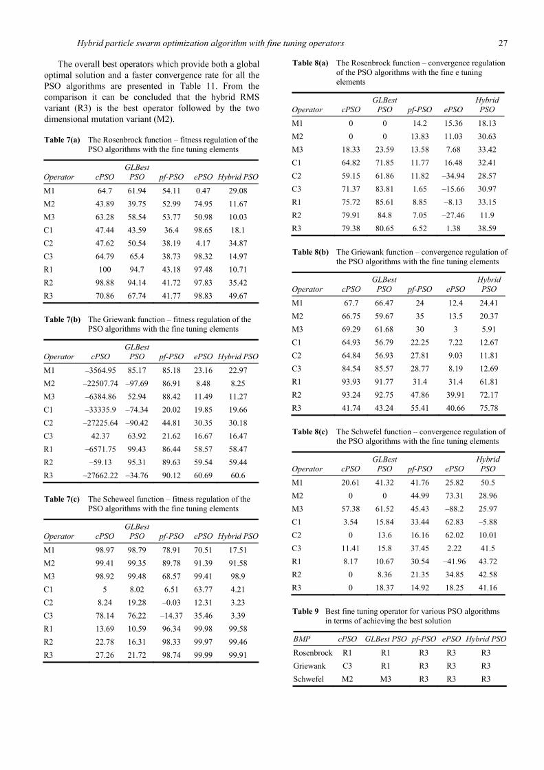
The fitness and convergence regulations of various PSO methods for the Rosenbrock, the Griewank, and the Schwefel functions are shown in the Tables 7(a) to 7(c) and Tables 8(a) to 8(c). From the fitness regulation comparison presented in Tables 7(a) to 7(c), the following conclusions can be drawn.

1 From the positive fitness regulation values obtained by all five PSO algorithms for the Rosenbrock function, it is understood that the presence of the fine tuning elements is unambiguously helpful to achieve better quality solutions.

2 For the Griewank function, the fine tuning elements are not useful for the cPSO method and GLBest PSO while the performance of the remaining methods (pf-PSO, ePSO, and hybrid PSO) is greatly improved, especially with the RMS variants.

3 For the Schwefel function, the near global optimum solution is achieved by cPSO and GLBest PSO algorithms with the help of mutation operators while for the remaining algorithms (pf-PSO, ePSO and hybrid PSO), the RMS variants accelerate their

performance in order to achieve a near global optimum value.

In the convergence regulation comparison presented in Tables 8(a) to 8(c), the RMS variants trigger all the five algorithms to converge faster into the global optimum value for the Rosenbrock and the Griewank functions. For the Rastrigin and the Schwefel functions, the mutation operators trigger almost all the PSO algorithms to reach a near global optimum value with a faster rate of convergence.

The best fine tuning operator for all the five PSO algorithms, in terms of achieving the best near global optimum solution and of a faster convergence rate are identified and presented in Tables 9 and 10. From Table 9, it can clearly be seen that the hybrid RMS variant (R3) is the best operator in accelerating the PSO algorithms towards the global optimal solution. From Table 10, it can be noticed that the hybrid RMS variant (R3) is the best operator in accelerating the PSO algorithms towards the global optimal solution for the Rosenbrock and the Griewank functions whereas the mutation operators (M2 and M3) provide a faster convergence rate for the Schwefel function.

Hybrid particle swarm optimization algorithm with fine tuning operators 27

The overall best operators which provide both a global optimal solution and a faster convergence rate for all the PSO algorithms are presented in Table 11. From the comparison it can be concluded that the hybrid RMS variant (R3) is the best operator followed by the two dimensional mutation variant (M2).

Table 7(a) The Rosenbrock function – fitness regulation of the PSO algorithms with the fine tuning elements

Operator cPSO GLBest

PSO pf-PSO ePSO Hybrid PSO

M1 64.7 61.94 54.11 0.47 29.08 M2 43.89 39.75 52.99 74.95 11.67 M3 63.28 58.54 53.77 50.98 10.03 C1 47.44 43.59 36.4 98.65 18.1 C2 47.62 50.54 38.19 4.17 34.87 C3 64.79 65.4 38.73 98.32 14.97 R1 100 94.7 43.18 97.48 10.71 R2 98.88 94.14 41.72 97.83 35.42 R3 70.86 67.74 41.77 98.83 49.67

Table 7(b) The Griewank function – fitness regulation of the PSO algorithms with the fine tuning elements

Operator cPSO GLBest

PSO pf-PSO ePSO Hybrid PSO

M1 –3564.95 85.17 85.18 23.16 22.97 M2 –22507.74 –97.69 86.91 8.48 8.25 M3 –6384.86 52.94 88.42 11.49 11.27 C1 –33335.9 –74.34 20.02 19.85 19.66 C2 –27225.64 –90.42 44.81 30.35 30.18 C3 42.37 63.92 21.62 16.67 16.47 R1 –6571.75 99.43 86.44 58.57 58.47 R2 –59.13 95.31 89.63 59.54 59.44 R3 –27662.22 –34.76 90.12 60.69 60.6

Table 7(c) The Scheweel function – fitness regulation of the PSO algorithms with the fine tuning elements

Operator cPSO GLBest

PSO pf-PSO ePSO Hybrid PSO

M1 98.97 98.79 78.91 70.51 17.51 M2 99.41 99.35 89.78 91.39 91.58 M3 98.92 99.48 68.57 99.41 98.9 C1 5 8.02 6.51 63.77 4.21 C2 8.24 19.28 –0.03 12.31 3.23 C3 78.14 76.22 –14.37 35.46 3.39 R1 13.69 10.59 96.34 99.98 99.58 R2 22.78 16.31 98.33 99.97 99.46 R3 27.26 21.72 98.74 99.99 99.91

Table 8(a) The Rosenbrock function – convergence regulation of the PSO algorithms with the fine e tuning elements

Operator cPSO GLBest

PSO pf-PSO ePSO Hybrid PSO

M1 0 0 14.2 15.36 18.13 M2 0 0 13.83 11.03 30.63 M3 18.33 23.59 13.58 7.68 33.42 C1 64.82 71.85 11.77 16.48 32.41 C2 59.15 61.86 11.82 –34.94 28.57 C3 71.37 83.81 1.65 –15.66 30.97 R1 75.72 85.61 8.85 –8.13 33.15 R2 79.91 84.8 7.05 –27.46 11.9 R3 79.38 80.65 6.52 1.38 38.59

Table 8(b) The Griewank function – convergence regulation of the PSO algorithms with the fine tuning elements

Operator cPSO GLBest

PSO pf-PSO ePSO Hybrid PSO

M1 67.7 66.47 24 12.4 24.41 M2 66.75 59.67 35 13.5 20.37 M3 69.29 61.68 30 3 5.91 C1 64.93 56.79 22.25 7.22 12.67 C2 64.84 56.93 27.81 9.03 11.81 C3 84.54 85.57 28.77 8.19 12.69 R1 93.93 91.77 31.4 31.4 61.81 R2 93.24 92.75 47.86 39.91 72.17 R3 41.74 43.24 55.41 40.66 75.78

Table 8(c) The Schwefel function – convergence regulation of the PSO algorithms with the fine tuning elements

Operator cPSO GLBest

PSO pf-PSO ePSO Hybrid PSO

M1 20.61 41.32 41.76 25.82 50.5 M2 0 0 44.99 73.31 28.96 M3 57.38 61.52 45.43 –88.2 25.97 C1 3.54 15.84 33.44 62.83 –5.88 C2 0 13.6 16.16 62.02 10.01 C3 11.41 15.8 37.45 2.22 41.5 R1 8.17 10.67 30.54 –41.96 43.72 R2 0 8.36 21.35 34.85 42.58 R3 0 18.37 14.92 18.25 41.16

Table 9 Best fine tuning operator for various PSO algorithms in terms of achieving the best solution

BMP cPSO GLBest PSO pf-PSO ePSO Hybrid PSO

Rosenbrock R1 R1 R3 R3 R3 Griewank C3 R1 R3 R3 R3 Schwefel M2 M3 R3 R3 R3

28 G. Ramana Murthy et al.

7 Comparisons with few recently developed PSO algorithms

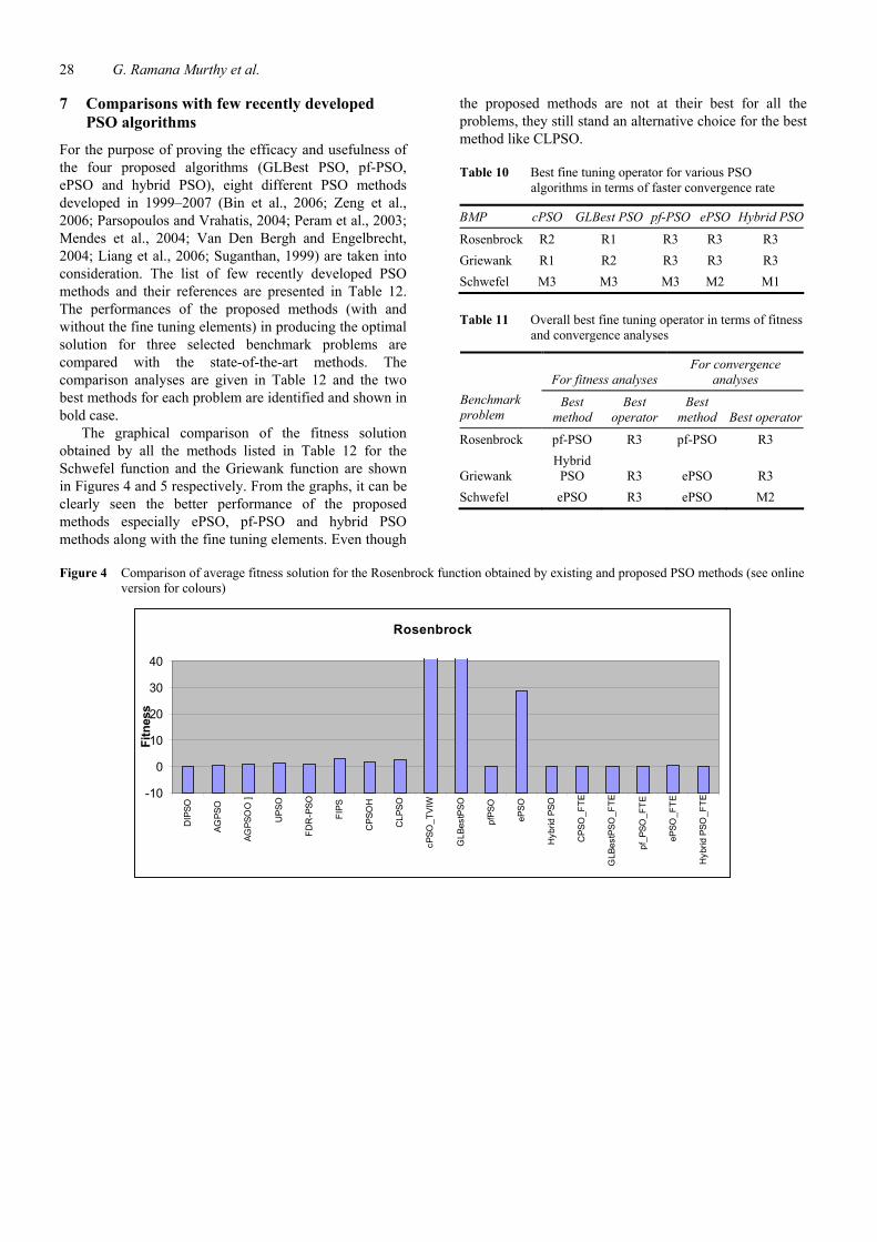
For the purpose of proving the efficacy and usefulness of the four proposed algorithms (GLBest PSO, pf-PSO, ePSO and hybrid PSO), eight different PSO methods developed in 1999–2007 (Bin et al., 2006; Zeng et al., 2006; Parsopoulos and Vrahatis, 2004; Peram et al., 2003; Mendes et al., 2004; Van Den Bergh and Engelbrecht, 2004; Liang et al., 2006; Suganthan, 1999) are taken into consideration. The list of few recently developed PSO methods and their references are presented in Table 12. The performances of the proposed methods (with and without the fine tuning elements) in producing the optimal solution for three selected benchmark problems are compared with the state-of-the-art methods. The comparison analyses are given in Table 12 and the two best methods for each problem are identified and shown in bold case.

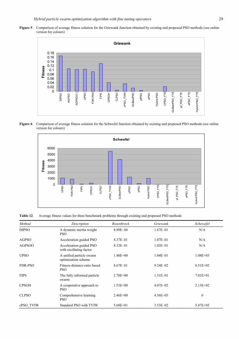
The graphical comparison of the fitness solution obtained by all the methods listed in Table 12 for the Schwefel function and the Griewank function are shown in Figures 4 and 5 respectively. From the graphs, it can be clearly seen the better performance of the proposed methods especially ePSO, pf-PSO and hybrid PSO methods along with the fine tuning elements. Even though

the proposed methods are not at their best for all the problems, they still stand an alternative choice for the best method like CLPSO.

Table 10 Best fine tuning operator for various PSO algorithms in terms of faster convergence rate

BMP cPSO GLBest PSO pf-PSO ePSO Hybrid PSO

Rosenbrock R2 R1 R3 R3 R3 Griewank R1 R2 R3 R3 R3 Schwefel M3 M3 M3 M2 M1

Table 11 Overall best fine tuning operator in terms of fitness and convergence analyses

For fitness analyses For convergence

analyses Benchmark problem

Best method

Best operator

Best method Best operator

Rosenbrock pf-PSO R3 pf-PSO R3

Griewank Hybrid

PSO R3 ePSO R3 Schwefel ePSO R3 ePSO M2

Figure 4 Comparison of average fitness solution for the Rosenbrock function obtained by existing and proposed PSO methods (see online version for colours)

Rosenbrock

-10

0

10

20

30

40

DIP

SO

AGPS

O

AGPS

OO

]

UPS

O

FDR

-PSO

FIPS

CPS

OH

CLP

SO

cPSO

_TVI

W

GLB

estP

SO

pfPS

O

ePSO

Hyb

rid P

SO

CPS

O_F

TE

GLB

estP

SO_F

TE

pf_P

SO_F

TE

ePSO

_FTE

Hyb

rid P

SO_F

TE

Fitn

ess

Hybrid particle swarm optimization algorithm with fine tuning operators 29

Figure 5 Comparison of average fitness solution for the Griewank function obtained by existing and proposed PSO methods (see online version for colours)

Griewank

00.020.040.060.080.1

0.120.140.160.18

DIP

SO

AGPS

O

AGPS

OO

]

UPS

O

FDR

-PSO

FIPS

CPS

OH

CLP

SO

cPSO

_TVI

W

GLB

estP

SO

pfPS

O

ePSO

Hyb

rid P

SO

CPS

O_F

TE

GLB

estP

SO_F

TE

pf_P

SO_F

TE

ePSO

_FTE

Hyb

rid P

SO_F

TE

Fitn

ess

Figure 6 Comparison of average fitness solution for the Schwefel function obtained by existing and proposed PSO methods (see online version for colours)

Schwefel

0

1000

2000

3000

4000

5000

6000

UPS

O

FDR

-PSO

FIPS

CPS

OH

CLP

SO

cPSO

_TVI

W

GLB

estP

SO

pfPS

O

ePSO

Hyb

rid P

SO

CPS

O_F

TE

GLB

estP

SO_F

TE

pf_P

SO_F

TE

ePSO

_FTE

Hyb

rid P

SO_F

TE

Fitn

ess

Table 12 Average fitness values for three benchmark problems through existing and proposed PSO methods

Method Description Rosenbrock Griewank Schewefel

DIPSO A dynamic inertia weight PSO

8.89E–04 1.67E–01 N/A

AGPSO Acceleration guided PSO 4.37E–01 1.07E–01 N/A AGPSOO Acceleration guided PSO

with oscillating factor 8.32E–01 1.02E–01 N/A

UPSO A unified particle swarm optimization scheme

1.40E+00 1.04E–01 1.08E+03

FDR-PSO Fitness-distance-ratio based PSO

8.67E–01 9.24E–02 8.51E+02

FIPS The fully informed particle swarm

2.78E+00 1.31E–01 7.01E+01

CPSOH A cooperative approach to PSO

1.53E+00 4.07E–02 2.13E+02

CLPSO Comprehensive learning PSO

2.46E+00 4.56E–03 0

cPSO_TVIW Standard PSO with TVIW 5.68E+01 3.53E–02 5.47E+03

30 G. Ramana Murthy et al.

Table 12 Average fitness values for three benchmark problems through existing and proposed PSO methods (continued)

Method Description Rosenbrock Griewank Schewefel

GLBest PSO Global local best PSO 5.36E+01 1.43E–02 4.11E+03 pf-PSO A parameter free PSO 5.50E–05 2.90E–03 1.21E+03 ePSO PSO like algorithm via

extrapolation 2.87E+01 8.30E–05 1.87E+02

Hybrid PSO Hybrid combination of pf-PSO and ePSO

5.34E–05 5.40E–05 9.99E+02

CPSO_FTE Standard PSO with the best fine tuning element

1.00E–04 2.30E–02 3.21E+01

GLBest PSO_FTE GLBest PSO with the best fine tuning element

1.00E–04 8.00E–05 2.14E+01

pf_PSO_FTE pf-PSO with the best fine tuning element

2.50E–05 1.00E–07 1.50E+01

ePSO_FTE ePSO with the best fine tuning element

3.36E–01 3.26E–05 1.59E–01

Hybrid PSO_FTE Hybrid PSO with the best fine tuning element

2.69E–05 2.13E–05 8.56E–01

8 Conclusions

The novel approach of hybrid PSO algorithm is proposed and its performance is demonstrated through a few benchmark testing problems. From the simulation results, it is observed that the proposed method exhibits the merits of both the pf-PSO and ePSO methods in solving the optimisation problems. In order to further accelerate the performance of the pf-PSO, ePSO and the hybrid PSO algorithms, nine fine tuning elements are incorporated individually along with all the mentioned PSO algorithms. The performance analyses of these three algorithms with the fine tuning elements are compared with those obtained through the cPSO and GLBest PSO methods. The best operators in terms of achieving the best optimal solution and faster convergence rate by various PSO algorithms for the three benchmark problems are identified. It can be concluded that the hybrid RMS variant (R3) is the best operator followed by two dimensional mutation variant (M2). The proposed methods are also compared with a few recently developed state-of-the-art methods. From the comparative analyses, it is evident that the performances of the proposed methods along with these best operators are more effective and competitive with the existing recently developed PSO methods.

References Angeline, P.J. (1998) ‘Evolutionary optimisation versus particle

swarm optimisation: philosophy and performance differences’, Evolutionary Programming VII, Lecture Notes in Computer Science, Vol. 1447, pp.601–610, Springer.

Angeline, P.J. (1999) ‘Using selection to improve particle swarm optimisation’, Proc. of IJCNN, Washington, USA, pp.84–89.

Bin, J., Lian, Z. and Gu, X. (2006) ‘A dynamic inertia weight particle swarm optimisation algorithm’, Chaos, Solutions & Fractals, doi: 10.1016/j.chaos.2006.09.063.

Eberhart, R.C. and Kennedy, J. (1995) ‘A new optimiser using particle swarm theory’, Proc. Sixth International Symposium on Micro Machine and Human Science, Nagoya, Japan, IEEE Service Center, Piscataway, NJ, pp.39–43.

Eberhart, R.C., Simpson, P. and Dobbins, R. (1996) Computational Intelligence PC Tools, Academic Press, Boston.

Gen, M. and Cheng, R. (1997) Genetic Algorithms and Engineering Design, John Wiley and Sons, Inc.

Kennedy, J. and Eberhart, R.C. (1995) ‘Particle swarm optimisation’, Proc IEEE International Conference on Neural Networks, Perth, Australia, IEEE Service Center, Piscataway, NJ, pp.1942–1948.

Lovbjerg, M., Ramussen, T.K. and Krink, T. (2001) ‘Hybrid particle swarm optimiser with breeding and sub populations’, Proc. of the Genetic and Evolutionary Computation Conference (GECCO), San Francisco, USA.

Liang, J.J., Qin, A., Suganthan, P.N. and Baskar, S. (2006) ‘Comprehensive learning particle swarm optimiser for global optimisation of multimodal functions’, IEEE Trans. Evolutionary Computation, Vol. 10, No. 3, pp.281–295.

Mendes, R., Kennedy, J. and Neves, J. (2004) ‘The fully informed particle swarm: simpler, maybe better’, IEEE Trans. Evolutionary Computation, Vol. 8, pp.204–210.

Michalewicz, Z. (1992) Genetic Algorithms + Data Structures = Evolution Programs, Springer, Verilog.

Parsopoulos, K.E. and Vrahatis, M.N. (2004) ‘UPSO – a unified particle swarm optimisation scheme’, in Lecture Series on Computational Sciences, pp.868–873.

Peram, T., Veeramachaneni, K. and Mohan, C.K. (2003) ‘Fitness-distance-ratio-based particle swarm optimisation’, in Proc. Swarm Intelligence Symp., pp.174–181.

Ratnaweera, A., Halgamuge, S.K. and Watson, C. (2004) ‘Self-organising hierarchical particle swarm optimiser with time-varying acceleration coefficient’, IEEE Transaction on Evolutionary Computation, Vol. 8, No. 3, pp.240–255.

Hybrid particle swarm optimization algorithm with fine tuning operators 31

Senthil Arumugam, M., Rao, M.V.C. and Aarthi, C. (2005) ‘Competitive approaches to PSO algorithms via new acceleration co-efficient variant with mutation operators’, Proceedings of the Fifth International Conference on Computational Intelligence and Multimedia Applications (ICCIMA), August, pp.225–230, IEEE Comp. Sci. Press.

Senthil Arumugam, M., Ramana Murthy, G., Rao, M.V.C. and Loo, C.K. (2007a) ‘A novel effective particle swarm optimisation like algorithm via extrapolation technique’, International Conference on Intelligent and Advanced Systems (ICIAS), Kuala Lumpur, Malaysia.

Senthil Arumugam, M., Rao, M.V.C. and Aarthi, C. (2007b) ‘A new and improved version of particle swarm optimisation algorithm with global-local best parameters’, Knowledge and Information Systems, Springer, doi: 10.1007/s10115-007-0109-z.

Senthil Arumugam, M., Rao, M.V.C. and Aarthi, C. (2007c) ‘A novel approach of parameter free particle swarm optimisation algorithm’, Second National Conference on Innovations in Communication and Computing (NCICC), January.

Shi, Y. and Eberhart, R.C. (1998a) ‘A modified particle swarm optimiser’, Proceedings of the IEEE International Conference on Evolutionary Computation, Anchorage, Alaska.

Shi, Y. and Eberhart, R.C. (1998b) ‘Parameter selection in particle swarm optimisation’, Evolutionary Programming VII, Lecture Notes in Computer Science, Vol. 1447, pp.591–600, Springer.

Suganthan, P.N. (1999) ‘Particle swarm optimiser with neighbourhood operator’, Proceedings of the 1999 Congress of Evolutionary Computation, Vol. 3, pp.1958–1962, IEEE Press.

Van Den Bergh, F. and Engelbrecht, A.P. (2004) ‘A cooperative approach to particle swarm optimisation’, IEEE Trans. Evolutionary Computation, Vol. 8, pp.225–239.

Zeng, J., Jie, J. and Hu, J. (2006) ‘Adaptive particle swarm optimisation guided by acceleration information’, International Conference on Computational Intelligence and Security, Vol. 1, pp.351–355.

Appendix

Benchmark problems

Function Name Search space (initialisation range) Global min

30 2 2 22 1

1( ) (100( ) ( 1) )i i i

if x x x x+

== − + −∑

Rosenbrock 100 100ix− ≤ ≤ (15 – 30) 2 (1, 1, 1,..., 1 )=0df

30 25

1 1

1( ) cos( ) 14000

ni

ii i i

xf x x= =

= − +∑ ∏ Griewank 600 600ix− ≤ ≤ (300 – 600) 5 (0, 0, 0,..., 0 )=0df

308

1( ) 418.98291 ( sin( | |))i i

if x n x x

== × + −∑

Schwefel 500 500ix− ≤ ≤ (–500 – 500) 8(420.9688,...,420.9688) 0f =