A hybrid method for unsteady inviscid fluid flow

This article appeared in a journal published by Elsevier. The attachedcopy is furnished to the author for internal non-commercial researchand education use, including for instruction at the authors institution

and sharing with colleagues.

Other uses, including reproduction and distribution, or selling orlicensing copies, or posting to personal, institutional or third party

websites are prohibited.

In most cases authors are permitted to post their version of thearticle (e.g. in Word or Tex form) to their personal website orinstitutional repository. Authors requiring further information

regarding Elsevier’s archiving and manuscript policies areencouraged to visit:

http://www.elsevier.com/copyright

http://www.elsevier.com/copyright

Author's personal copy

A hybrid method for unsteady inviscid fluid flow q

Jan Nordström a,b,c,*, Frank Ham d, Mohammad Shoeybi d, Edwin van der Weide e,g, Magnus Svärd d,f,Ken Mattsson a,d, Gianluca Iaccarino d, Jing Gong a

a Department of Information Technology, Scientific Computing, Uppsala University, SE-751 05 Uppsala, Swedenb Department of Aeronautical and Vehicle Engineering, KTH, The Royal Institute of Technology, SE-100 44 Stockholm, Swedenc Department of Computational Physics, FOI, The Swedish Defence Research Agency, SE-164 90 Stockholm, Swedend Center for Turbulence Research, CTR, Building 500, Stanford University, Stanford, CA 94305-3035, USAe Department of Aeronautics and Astronautics, Stanford University, Stanford, CA 94305-4035, USAf Center of Mathematics for Applications, University of Oslo, P.B. 1053 Blindern N-0316 Oslo, Norwayg Faculty of Engineering Technology, University of Twente, P.O. Box 217, 7500 AE Enschede, The Netherlands

a r t i c l e i n f o

Article history:Received 27 November 2007Received in revised form 17 September 2008Accepted 18 September 2008Available online 17 October 2008

a b s t r a c t

We show how a stable and accurate hybrid procedure for fluid flow can be constructed. Two separatesolvers, one using high order finite difference methods and another using the node-centered unstruc-tured finite volume method are coupled in a truly stable way. The two flow solvers run independentlyand receive and send information from each other by using a third coupling code. Exact solutions tothe Euler equations are used to verify the accuracy and stability of the new computational procedure.We also demonstrate the capability of the new procedure in a calculation of the flow in and around amodel of a coral.

� 2008 Elsevier Ltd. All rights reserved.

1. Introduction

The generation and transportation of vortexes from wing-tips,rotors and wind turbines, and the generation and propagation ofsound from aircraft, cars and submarines require methods thatcan handle locally highly nonlinear phenomena in complex geom-etries as well as efficient and accurate signal transportation in do-mains with smooth flow and geometries. This technique can alsobe used in adapting an essentially structured mesh to a curvedshock.

The combination of finite volume methods on unstructuredgrids (for the part with nonlinear phenomena and complex geom-etries) and high-order finite difference methods on structuredgrids (for the wave propagation part) meet these demands. Inmany cases separate stand-alone codes using these methods alsoexist. In this paper we will show how to combine the finite volumeand finite difference method and the related codes into a practicalprocedure.

1.1. Background, main ideas and previous results

There are essentially two different types of hybrid methods. Themost common one employs different governing equations in differ-

ent parts of the computational domain. A typical example is noisegenerated in an isolated part of the flow, considered as the soundsource. The nonlinear phenomenon in the complex geometry is of-ten computed by the Euler or Navier–Stokes equations. The soundpropagation to the far field is considered governed by the linearwave equation with source terms from the Euler or Navier–Stokescalculation. This type of hybrid method is discussed in [1,2].

In this paper we consider another type of hybrid method thatuse the same governing equations (in this case the compressibleEuler equations) in the whole computational domain, not just closeto the source. The word hybrid refers to the use of different numer-ical methods in different parts of the computational domain.Examples of this type of hybrid method can be found in [3,4]. Inthis type of coupling procedure (provided that accurate data areknown) a stable and accurate numerical procedure does sufficefor convergence to the true solution.

Many of the flow phenomena that we are interested in last forlong times and information propagate over long distances. Strictstability which prevents error growth on realistic mesh sizes, isvery important for calculations over long times. We have derivedand studied strictly stable unstructured finite volume methods(see [5–7]) and high-order finite difference methods (see [8–13]) for both hyperbolic, parabolic and incompletely parabolicproblems. These methods employ so-called summation-by-partsoperators and impose the boundary conditions weakly (see[5,14]).

In [15] it was proved that a specific interface procedureconnecting finite difference methods and finite volume methods

0045-7930/$ - see front matter � 2008 Elsevier Ltd. All rights reserved.doi:10.1016/j.compfluid.2008.09.010

q This work was carried out while the first and last author were visiting CTR.* Corresponding author. Address: Department of Information Technology, Scien-

tific Computing, Uppsala University, SE-751 05 Uppsala, Sweden.E-mail address: [email protected] (J. Nordström).

Computers & Fluids 38 (2009) 875–882

Contents lists available at ScienceDirect

Computers & Fluids

journal homepage: www.elsevier .com/ locate /compfluid


is stable for hyperbolic systems of equations. This study will relyheavily on these results and we will apply the theoretical resultsto the Euler equations. We will demonstrate that the theoretical re-sults in [15] in combination with two existing efficient codes and athird coupling code will lead to an efficient and practical computa-tional tool.

A three-dimensional code (CDP) that uses the node-centered fi-nite volume method mentioned above has been developed in theCenter for Turbulence Research (CTR) at Stanford University, see[16]. Another three-dimensional multi-block code (NSSUS) thatuses the finite difference technique discussed above is availableat the Department of Aeronautics & Astronautics at Stanford Uni-versity, see [17]. These codes compute approximations to the Euleror Navier–Stokes equations and are the initial building blocks forthe new hybrid method. A third coupling code (Chimps-lite, a sim-plified version of Chimps [18]) will administer the coupling proce-dure and make it possible for the two solvers to communicate in anefficient and scalable way.

The rest of this paper will proceed as follows. For complete-ness, we shortly review the results in [15] in Section 2. In Sec-tion 3 we describe the two sets of computational solvers andthe specific coupling code. In Section 4 we validate the computa-tional procedure against exact solutions and show the abilityto cope with complex geometries and high accuracy require-ments. Finally, we draw conclusions and discuss future work inSection 5.

2. Analysis

To introduce our technique (see [15]) we consider the hyper-bolic system

ut þ Aux þ Buy ¼ 0; �1 6 x 6 1; 0 6 y 6 1 ð1Þ

with suitable initial and boundary conditions. A and B are constantsymmetric matrices with k rows and columns. We consider a sim-plified computational domain that is divided into two sub-domains.A so-called node-centered unstructured finite volume method willbe used to discretize (1) on sub-domain ½�1;0� � ½0;1� with anunstructured mesh, while a high-order finite difference method willbe used on sub-domain ½0;1� � ½0;1� with a structured mesh, seeFig. 1. The fact that the unknowns in the finite volume and the finitedifference methods are located in the nodes and can be co-locatedat the interface is a key ingredient in the coupling procedure we willpresent below.

2.1. The node-centered finite volume method

The so-called node-centered finite volume method is used inthis paper (see [19–23] for more details). In [5,15] it was shownthat the semi-discrete finite volume form of (1) on sub-domain½�1;0� � ½0;1� can be written,

ut þ DLx � A

n ouþ DL

y � Bn o

u ¼ SATLI ðuI � vIÞ þ SATL

O: ð2Þ

The difference operators and the penalty term that imposes theinterface conditions have the form (see [15])

DLx ¼ ðP

LÞ�1Q Lx; DL

y ¼ ðPLÞ�1Q L

y; SATLI ¼ ðPLÞ�1ðEL

I ÞT YI

h i� RL:

SATLO imposes the outer boundary conditions weakly. uI and vI

are vectors which represent u and v (v is the discrete finite differ-ence solution that will be presented below) on the interface,respectively. EL

I is a projection matrix which maps u to uI such thatuI ¼ ðEL

I � IkÞu. The non-zero components of ELI have the value 1

and appear at the interface. Ik is the k� k identity matrix. YI � RL

is a penalty matrix that will be determined below by stabilityrequirements.

PL is a positive diagonal m�m matrix with the control volumesXi on the diagonal. QL

x and QLy are almost skew symmetric m�m

matrices and satisfy

QLx þ ðQ

LxÞ

T ¼ Y; Q Ly þ ðQ

LyÞ

T ¼ X; ð3Þ

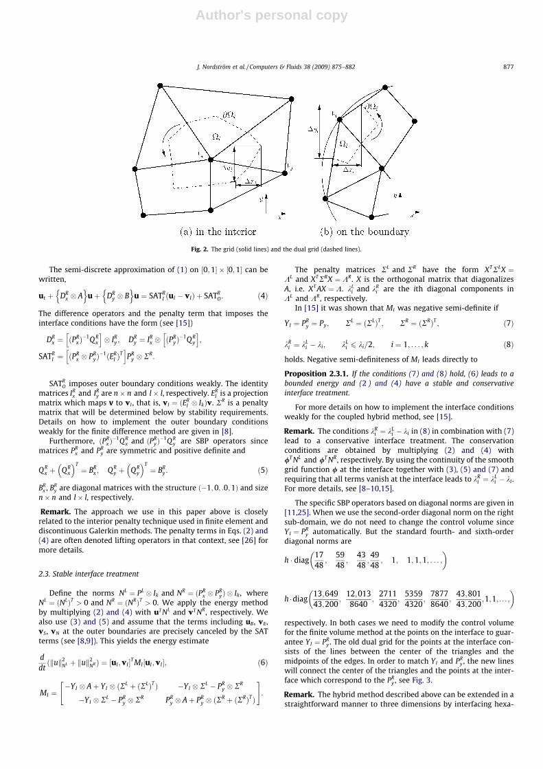
where the non-zero elements in Y and X are Dyi, �Dxi and corre-spond to the boundary points. For the definition of Dxj and Dyj,see Fig. 2. The part of the penalty term SATL

I denoted by YI is therestriction of Y to the interface. For more details on the SBP proper-ties of the finite volume scheme and how to implement the outerboundary conditions weakly, see [5].

2.2. The high-order finite difference method

The high-order finite difference method used in this paper isdescribed in [8–13]. Consider the sub-domain ½0;1� � ½0;1� with astructured mesh of n� l points. The finite difference approxima-tion of u at the grid point ðxi; yjÞ is a k� 1 vector denoted vij. Weorganize the solution in the global vector v ¼ ½v11; . . . ;v1l;v21; . . .,v2l; . . . ;vn1; . . . ;vnl�T . vx and vy are approximations of ux and uy

and are approximated using the high-order accurate SBP operatorsfor the first derivative that were constructed in [24,25].

West

North

East

South

y=1

x=1 x= 1

U V

Interface

y=0

Fig. 1. The hybrid mesh on the computational domain.

876 J. Nordström et al. / Computers & Fluids 38 (2009) 875–882


The semi-discrete approximation of (1) on ½0;1� � ½0;1� can bewritten,

ut þ DRx � A

n ouþ DR

y � Bn o

u ¼ SATRI ðuI � vIÞ þ SATR

O: ð4Þ

The difference operators and the penalty term that imposes theinterface conditions have the form (see [15])

DRx ¼ ðPR

x Þ�1Q R

x

h i� IR

y ; DRy ¼ IR

x � ðPRyÞ�1Q R

y

h i;

SATRI ¼ ðPR

x � PRyÞ�1ðER

I ÞT

h iPR

y � RR:

SATRO imposes outer boundary conditions weakly. The identity

matrices IRx and IR

y are n� n and l� l, respectively. ERI is a projection

matrix which maps v to vI , that is, vI ¼ ðERI � IkÞv. RR is a penalty

matrix that will be determined below by stability requirements.Details on how to implement the outer boundary conditionsweakly for the finite difference method are given in [8].

Furthermore, ðPRx Þ�1Q R

x and ðPRyÞ�1Q R

y are SBP operators sincematrices PR

x and PRy are symmetric and positive definite and

Q Rx þ Q R

x

� �T¼ BR

x ; QRy þ QR

y

� �T¼ BR

y : ð5Þ

BRx , BR

y are diagonal matrices with the structure ð�1;0; :0;1Þ and sizen� n and l� l, respectively.

Remark. The approach we use in this paper above is closelyrelated to the interior penalty technique used in finite element anddiscontinuous Galerkin methods. The penalty terms in Eqs. (2) and(4) are often denoted lifting operators in that context, see [26] formore details.

2.3. Stable interface treatment

Define the norms NL ¼ PL � Ik and NR ¼ ðPRx � PR

yÞ � Ik, whereNL ¼ ðNLÞT > 0 and NR ¼ ðNRÞT > 0. We apply the energy methodby multiplying (2) and (4) with uT NL and vT NR, respectively. Wealso use (3) and (5) and assume that the terms including uB, vE,vS, vN at the outer boundaries are precisely canceled by the SATterms (see [8,9]). This yields the energy estimate

ddtðkuk2

NL þ kuk2NR Þ ¼ ½uI;vI�T MI½uI;vI�; ð6Þ

MI ¼�YI � Aþ YI � ðRL þ ðRLÞTÞ �YI � RL � PR

y � RR

�YI � RL � PRy � RR PR

y � Aþ PRy � ðR

R þ ðRRÞTÞ

" #:

The penalty matrices RL and RR have the form XTRLX ¼KL and XTRRX ¼ KR. X is the orthogonal matrix that diagonalizesA, i.e. XT AX ¼ K. kL

i and kRi are the ith diagonal components in

KL and KR, respectively.In [15] it was shown that MI was negative semi-definite if

YI ¼ PRy ¼ Py; RL ¼ ðRLÞT ; RR ¼ ðRRÞT ; ð7Þ

kRi ¼ kL

i � ki; kLi 6 ki=2; i ¼ 1; . . . ; k ð8Þ

holds. Negative semi-definiteness of MI leads directly to

Proposition 2.3.1. If the conditions (7) and (8) hold, (6) leads to abounded energy and (2 ) and (4) have a stable and conservativeinterface treatment.

For more details on how to implement the interface conditionsweakly for the coupled hybrid method, see [15].

Remark. The conditions kRi ¼ kL

i � ki in (8) in combination with (7)lead to a conservative interface treatment. The conservationconditions are obtained by multiplying (2) and (4) with/T NL and /T NR, respectively. By using the continuity of the smoothgrid function / at the interface together with (3), (5) and (7) andrequiring that all terms vanish at the interface leads to kR

i ¼ kLi � ki.

For more details, see [8–10,15].

The specific SBP operators based on diagonal norms are given in[11,25]. When we use the second-order diagonal norm on the rightsub-domain, we do not need to change the control volume sinceYI ¼ PR

y automatically. But the standard fourth- and sixth-orderdiagonal norms are

h � diag1748

;5948

;4348

;4948

; 1; 1;1;1; . . . ;

� �

h �diag13;64943;200

;12;0138640

;27114320

;53594320

;78778640

;43;80143;200

;1;1; . . . ;� �

respectively. In both cases we need to modify the control volumefor the finite volume method at the points on the interface to guar-antee YI ¼ PR

y . The old dual grid for the points at the interface con-sists of the lines between the center of the triangles and themidpoints of the edges. In order to match YI and PR

y , the new lineswill connect the center of the triangles and the points at the inter-face which correspond to the PR

y , see Fig. 3.

Remark. The hybrid method described above can be extended in astraightforward manner to three dimensions by interfacing hexa-

Fig. 2. The grid (solid lines) and the dual grid (dashed lines).

J. Nordström et al. / Computers & Fluids 38 (2009) 875–882 877


hedra from the structured side with pyramids on the unstructuredside. Stability will be obtained by modifying the correspondingtwo-dimensional finite volume norm (choose the dual grid prop-erly) to match the two-dimensional finite difference norm.

3. Computational tools

The node-centered finite volume code (CDP) and the high orderfinite difference code (NSSUS) are the initial building blocks for thenew hybrid method. Both CDP and NSSUSS are stand-alone codesthat computes approximations to the Euler or Navier–Stokes equa-

tions. The codes are node-based and use SBP operators and penaltytechniques for imposing the boundary and interface conditionsweakly. This numerical technique enables coupling of the twocodes by sending the value of the dependent variables in the nodeslocated on the interface to the other code and at the same timereceiving the co-located data at the interface from the other code.Each code provides boundary data to the other code.

A third coupling code (Chimps-lite) will administer the couplingprocedure and make it possible for the two solvers to communicatein a correct way. Chimps-lite identifies co-located nodes in a pre-processing step and during the execution it manages the exchangeof data between CDP and NSSUS, at each stage in the explicit time-integration procedure [27]. See Fig. 4 for a schematic illustration.

Fig. 3. The modified control volumes for the points on the interface.

Fig. 4. Schematic interface communication.



The development of Chimps-lite is an essential new ingredient thatwill take the coupling idea from a theoretical concept to a practi-cally useful tool for fluid flow investigations. It will be discussedin some detail below.

3.1. Chimps-lite and parallel implementation consideration

In addition to the mathematical and numerical foundation pre-sented previously, the development of a massively parallel (say1000+ processor) hybrid simulation capability requires a fast, scal-able model for the regular exchange of data between the varioussolvers.

One option is to write a new hybrid solver that merges thedesired solver capabilities and includes an additional layer ofcommunication associated with the interfaces. While this optionwill allow us to continue to run in the single-program-multiple-data (SPMD) mode that has emerged as the dominant model forlarge-scale parallel computation, it has the down-side of requir-ing major modifications to both codes. In some cases the codeswill be written in different languages. There may be globalname-space conflicts that prevent us from simply writing acommon ‘‘main” that calls the appropriate solver as a ‘‘subrou-tine”. The required re-coding will invariably introduce additionalbugs that must be corrected. When the stand-alone codes havehad 10s or even hundreds of man-years of development, verifica-tion, and validation, this level of intervention is normallyunacceptable.

An alternative approach is to run both codes in a stand-alonemode under one multiple-program-multiple-data (MPMD) session,and use an additional library of routines to handle the interfacecommunication. This approach requires minimal modifications tothe codes, and is the one we follow in the present implementationusing a simplified version of the CHIMPS coupling library [18]called CHIMPS-lite.

In this model, only two minor modifications are required to theparticipating codes – one associated with the initialization of MPIand the other with exchanging data prior to application of theinterface conditions. These modifications are described in the fol-lowing subsections. Note that the MPI commands in the next sec-tion are shell dependent.

3.2. Communicator splitting

Many MPI environments support running MPMD from the com-mand line. For example, the command:

mpirun -np 10 code1: -np 25 code2

will run code1 on 10 processors, and code2 on 25 processors (i.e.35 processors total), all having a common world communicator.For systems that do not support this model, the same thing canbe accomplished through modifications to the job submissionscript, or even by using a simple shell script that parses the proces-sor number normally available as an environment variable. Forexample:

mpirun -np 35 mpmd.sh

where mpmd.sh is the following:

#!/bin/bash

if [$ PROCID -le 9]

then./code1

else./code2

fi

In either case, both codes will start up with a common worldcommunicator that must be split before normal execution can con-tinue. This splitting is the first modification required in the codes.It can be done at the point where the routine MPI_Init() wouldnormally be called. Instead, both codes should call a common rou-tine in the coupling library that takes a unique key or name fromeach solver, calls MPI_Init(), and then splits the communicatorbased on the key, returning a unique communicator to each solver.All local MPI routines in the solvers should then use this split com-municator for their local MPI calls, and not MPI_COMM_WORLD. Thiscall will of course be collective and blocking.

3.3. Data exchange

In the context of SBP/SAT codes, the application of interfaceconditions is very similar to boundary conditions except that thedata used in forming the penalty terms comes from the point-matched interface data associated with the other solver. The sec-ond modification to the participating codes is thus an exchangeof interface data prior to forming the interface penalty terms. Forthe present computations involving fixed grids and conformalinterfaces, the building of the communication pattern associatedwith this exchange can be considered a preprocessing step becauseit remains fixed throughout the simulation. Consequently the sca-lability of the searches is not critical, however, we have used thescalable search routines described in [18] to locate matchingpoints.

On the first call to the data exchange, both codes provide the listof coordinates of their interface points to CHIMPS-lite, which thenproceeds to build the communication pattern associated with thedata exchange based on matching point coordinate locations be-tween solvers (within a small tolerance). On subsequent calls,the same communication pattern can be reused, making the costof each exchange very modest. Fig. 4 illustrates this process sche-matically. By using the CHIMPS-lite routines to build the commu-nication pattern and manage the data exchanges, it is nevernecessary for the solvers to have any direct knowledge of eachother’s partitioning details.

4. Numerical calculations

The coupling procedure applied to the scalar advection equationwas extensively tested and validated in [15]. Here we will makesure the theoretical results derived above for the symmetrized con-stant coefficient system also apply to the fully non-linear Eulerequations.

Remark. The stability analysis above was done on a system withconstant symmetric matrices. Here we multiply the constantcoefficient version of the Euler equations with a symmetrizingmatrix from the left. We use the symmetrizer derived in [28]. Oncethe penalty matrices are obtained, the whole system is trans-formed back to non-symmetric form and implemented.

4.1. Validation

The coupling procedure applied to the scalar advection equationwas extensively tested and validated in [15]. Here we will makesure these results also apply to a non-linear system of equations(the Euler equations). We calculate the propagation of a vortexwith constant velocity (an exact solution to the Euler equations)across an interface. A typical mesh for this calculation is shownin Fig. 5. We use the explicit three-stage third-order time-steppingscheme of Le and Moin [27]. The solution is advanced with a globaltime-step based on the smallest grid size in both domains.



The accuracy of the coupled procedure for various orders ofaccuracy of the NSSUS finite difference code is shown in Tables1–5. The errors are computed when the vortex is centered at theinterface. The presence of second-order errors produced by CDPwill limit the overall convergence rate to 2 even if NSSUS runs withhigher accuracy. Similar results have been produced for variouscombinations of directions and orders of accuracy in NSSUS andthey indicate that the procedure converges with the appropriaterate.

As can be seen in the tables, the highest gain in accuracy isobtained for the case where the vortex propagates from the high-order accurate NSSUS region into the second-order accurate CDPregion. We illustrate that in Fig. 6 which shows the solution andthe error for the coupling between NSSUS (second and fourth or-der) and CDP. The error levels in both calculations are very small(of the order 10�4). The error levels for the second-order NSSUS

are visible long before the vortex hits the interface. For thefourth-order case, nothing can be seen until the vortex reachesthe interface.

4.2. An application

The new hybrid method can handle nonlinear phenomena incomplex geometries as well as efficient and accurate signal trans-portation in domains with smooth flow and geometries. Wedemonstrate that capability in a calculation of the flow througha two-dimensional model of a coral. In this calculation we usethe sixth-order accurate version of NSSUS. The geometry andthe corresponding mesh can be seen in Fig. 7. The center of thecoral is at ðx; yÞ ¼ ð0;0Þ. The interface is located at x ¼ 0:6. The cal-culation proceeds as follows. First we compute a steady statesolution. Next, we take the steady state solution and add the vor-tex centered at ðx; yÞ ¼ ð�1:5;0Þ. That is our initial solution, seeFig. 8a.

As time passes, the vortex propagates through the coral (in theunstructured finite volume region) and sits at t ¼ 2:6 just at theinterface leaving the coral, see Fig. 8b. The shape of the vortex ismodified by the coral. At t ¼ 3:6 the vortex has left the coral regionand is now propagating (with sixth-order accuracy) downstream,see Fig. 9a. The vortex seems to return to it’s original form. Finally,at t ¼ 4:4 the vortex is approaching the right boundary and it iseven closer to it’s original shape, see Fig. 9b.

Table 1Error as vortex propagate from second-order NSSUS region intosecond-order CDPregion.

N log lðNSSUSÞ2

� �qðNSSUSÞ log lðCDPÞ

2

� �qðCDPÞ

51 � 51 �2.88 – �3.22 –101 � 101 �3.50 2.06 �3.77 1.83201 � 201 �4.11 2.03 �4.36 1.96401 � 401 �4.71 2.00 �4.96 1.99

Fig. 5. Mesh for the accuracy validation of the interface procedure.

Table 3Error as vortex propagate from 6th-order NSSUS region into second-order CDP region.

N log lðNSSUSÞ2


2

� �qðCDPÞ

51 � 51 �3.89 – �3.82 –101 � 101 �4.92 3.41 �4.41 1.98201 � 201 �5.68 2.53 �5.01 2.00401 � 401 �6.31 2.11 �5.62 2.02

Table 2Error as vortex propagate from fourth-order NSSUS into region second-order CDPregion.

N log lðNSSUSÞ2


2

� �qðCDPÞ

51 � 51 �4.00 – �3.82 –101 � 101 �4.89 2.96 �4.41 1.98201 � 201 �5.63 2.47 �5.01 2.00401 � 401 �6.30 2.21 �5.62 2.02

Table 4Error as vortex propagate from second-order CDP region into second-order NSSUSregion.

N log lðCDPÞ2

� �qðCDPÞ log lðNSSUSÞ

2

� �qðNSSUSÞ

51 � 51 �3.03 – �3.01 –101 � 101 �3.65 2.05 �3.60 1.93201 � 201 �4.25 2.00 �4.19 1.98

Table 5Error as vortex propagate from second-order CDP region into fourth-order NSSUSregion.

N log lðCDPÞ2

� �qðCDPÞ log lðNSSUSÞ

2

� �qðNSSUSÞ

51 � 51 �3.03 – �3.06 –101 � 101 �3.65 2.05 �3.65 1.95201 � 201 �4.25 2.00 �4.25 1.98



Fig. 6. Vortex propagating over interface. The columns correspond to three different times. The first row show the density distribution. The second and third rows show thedensity error for the second and fourth-order NSSUS coupled to CDP, respectively.

Fig. 7. Geometry and grid topology of hybrid calculation around coral.

Fig. 8. Time sequence for the vortex–coral interaction, t ¼ 0:0 and t ¼ 2:3.



5. Conclusions and future work

We have developed a hybrid method constructed by the cou-pling of two stand-alone existing CFD codes. The coupling isadministered by a third separate coupling code.

The hybrid method allows for individual development of thestand-alone CFD codes. No development with consideration tothe other code is required since the CFD codes only communicatewith each other through the third coupling code.

We have demonstrated that the hybrid method is an accurate,efficient and a practically useful computational tool that can han-dle complex geometries as well as wave propagation phenomena.

The next step involves including the viscous terms. Initial workin that direction is ongoing, see [29]. With an efficient hybridmethod for the Navier–Stokes equations, large scale flow problemsin complex geometries including wave propagation effects, can beanalyzed.

References

[1] Lyrintzis AS. Review: the use of Kirchhoff’s method in computationalaeroacoustics. J Fluids Eng 1994;116:665–76.

[2] Wells VL, Renaut RA. Computing aerodynamically generated noise. Annu RevFluid Mech 1997;29:161–99.

[3] Burbeau A, Sagaut P. A dynamic p-adaptive discontinuous Galerkin method forviscous flow with shocks. Comput Fluids 2005;34(4–5):401–17.

[4] Rylander T, Bondeson A. Stable FEM-FDTD hybrid method for Maxwell’sequations. Comput Phys Commun 2000;125:75–82.

[5] Nordström J, Forsberg K, Adamsson C, Eliasson P. Finite volume, methodsunstructured meshes and strict stability. Appl Numer Math 2003;45:453–73.

[6] Svärd M, Nordström J. Stability of finite volume approximations for theLaplacian operator on quadrilateral and triangular grids. Appl Numer Math2004;51:101–25.

[7] Svärd M, Gong J, Nordström J. Strictly stable artificial dissipation for finitevolume schemes. Appl Numer Math 2007;56(12):1481–90.

[8] Carpenter MH, Nordstrom J, Gottlieb D. A stable and conservative interfacetreatment of arbitrary spatial accuracy. J Comput Phys 1999;148:341–6.

[9] Nordström J, Carpenter MH. Boundary and interface conditions for high orderfinite difference methods applied to the Euler and Navier–Stokes equations. JComput Phys 1999;148:621–45.

[10] Nordström J, Carpenter MH. High-order finite difference methods,multidimensional linear problems and curvilinear coordinates. J ComputPhys 2001;173:149–74.

[11] Mattsson K, Nordström J. Summation by parts operators for finite differenceapproximations of second derivatives. J Comput Phys 2004;199:503–40.

[12] Svärd M, Nordström J. On the order of accuracy for difference approximationsof initial-boundary value problems. J Comput Phys 2006;218(1):333–52.

[13] Svärd M, Carpenter MH, Nordström J. A stable high-order finite differencescheme for the compressible Navier–Stokes equations: far-field boundaryconditions. J Comput Phys 2007;225(1):1020–38.

[14] Carpenter MH, Gottlieb D, Abarbanel S. Time-stable boundary conditions forfinite-difference schemes solving hyperbolic systems: methodology andapplication to high-order compact schemes. J Comput Phys 1994;129(2).

[15] Nordström J, Gong Jing. A stable hybrid method for hyperbolic problems.J Comput Phys 2006;212(2):436–53.

[16] Ham F, Mattsson K, Iaccarino G. Accurate and stable finite volume operatorsfor unstructured flow solvers. Annual Research Briefs, CTR, StanfordUniversity; 2006.

[17] Svard M, Van der Weide E. Stable and high-order accurate finite differenceschemes on singular grids. Annual Research Briefs, CTR, Stanford University;2006.

[18] J.J. Alonso, S. Hahn, F. Ham, M. Herrmann, G. Iaccarino, G. Kalitzin, P.LeGresley, K. Mattsson, G. Medic, P. Moin, H. Pitsch, J. Schluter, M. Svard,E. van der Weide, D. You, and X. Wu, Chimps: A high-performancescalable module for multi-physics simulations, AIAA Paper 2006-5274,2006.

[19] T. Gerhold, O. Friedrich, and J. Evans, Calculation of complex three-dimensional configurations employing the DLR-s-code, AIAA Paper 97-0167,1997.

[20] Haselbacher A, McGuirk JJ, Page GJ. Finite volume discretization aspects forviscous flows on mixed unstructured grids. AIAA J 1999;37(2).

[21] Mavriplis DJ. Accurate multigrid solution of the Euler equations onunstructured and adaptive meshes. AIAA J 1990;28(2).

[22] Mavriplis DJ, Venkatakrishnan V. A unified multigrid solver for the Navier–Stokes equations on mixed element meshes, Technical report, Institute forComputer Applications in Science and Engineering; 1995.

[23] Weiss JM, Maruszewski JP, Smith WA. Implicit solution ofpreconditioned Navier–Stokes equations using algebraic multigrid.AIAA J 1999;37(1).

[24] Kreiss H-O, Scherer G. Finite element and finite difference methods forhyperbolic partial differential equations. In: De Boor C, editor. Mathematicalaspects of finite elements in partial differential equation. New York: AcademicPress; 1974.

[25] Strand B. Summation by parts for finite difference approximation for d/dx. JComput Phys 1994;110(1):47–67.

[26] Arnold DN, Brezzi F, Cockburn B, Marini LD. Unified analysis of discontinuousGalerkin methods for eliptic problems. SIAM J Numer Anal2002;39(5):1749–79.

[27] Le H, Moin P. An improvement of fractional step methods for theincompressible Navier–Stokes equations. J Comput Phys 1991;92:369–79.

[28] Abarbanel S, Gottlieb D. Optimal time splitting for two- and three-dimensionalNavier–Stokes equations with mixed derivatives. J Comput Phys1981;41:1–43.

[29] Gong J, Nordström J. A stable and efficient hybrid scheme for viscous problemsin complex geometries. J Comput Phys 2007;226:1291–309.

Fig. 9. Time sequence for the vortex–coral interaction, t ¼ 3:6 and t ¼ 4:4.


A hybrid method for unsteady inviscid fluid flow

Documents