A Hybrid Graph Representation for Recursive Backtracking Algorithms

A Hybrid Graph Representation for Recursive

Backtracking Algorithms

Faisal N. Abu-Khzam1,�, Michael A. Langston2,Amer E. Mouawad1, and Clinton P. Nolan2,��

1 Department of Computer Science and MathematicsLebanese American University

Beirut, Lebanon{faisal.abukhzam,amer.mouawad}@lau.edu.lb

http://www.csm.lau.edu.lb/fabukhzam2 Department of Electrical Engineering and Computer Science

University of TennesseeKnoxville, TN 37996-3450 USA

{langston,nolan}@eecs.utk.eduhttp://www.cs.utk.edu/~langston

Abstract. Many exact algorithms for NP-hard graph problems adoptthe old Davis-Putman branch-and-reduce paradigm. The performanceof these algorithms often suffers from the increasing number of graphmodifications, such as deletions, that reduce the problem instance andhave to be “taken back” frequently during the search process. The use ofefficient data structures is necessary for fast graph modification modulesas well as fast take-back procedures. In this paper, we investigate prac-tical implementation-based aspects of exact algorithms by providing ahybrid graph representation that addresses the take-back challenge andcombines the advantage of O(1) adjacency-queries in adjacency-matriceswith the advantage of efficient neighborhood traversal in adjacency-lists.

Keywords: data structures, exact algorithms, recursive backtracking,vertex cover, dominating set.

1 Introduction

The interest in exact algorithms for hard graph problems is now more thanfifty years old. Countless exact and parameterized algorithms with improvedworst-case run-times have been developed in the last several years only [5,6,11].However, most research in this area concentrates on worst-case analysis, dealingwith data structure design and implementation from an abstract level only.� This research has been supported in part by the research council of the Lebanese

American University.�� This research has been supported in part by the U.S. Department of Energy under

the EPSCoR Laboratory Partnership Program. It has used resources of the NationalEnergy Research Scientific Computing Center, which is supported by the Office ofScience under Contract No. DE-AC02-05CH11231.

D.T. Lee, D.Z. Chen, and S. Ying (Eds.): FAW 2010, LNCS 6213, pp. 136–147, 2010.c© Springer-Verlag Berlin Heidelberg 2010

Hybrid Graph Representation 137

In this paper, we investigate the practical aspects of some exact algorithmsfor NP-hard graph-theoretic problems. The majority of such exact algorithmsadopt the classical recursive backtracking methodology, with the adjacency-listor adjacency-matrix as default graph representation. We present a hybrid graphrepresentation that trades space for time to combine the advantage of O(1)adjacency-queries in adjacency-matrices and the advantage of efficient neighbor-hood traversal in adjacency-lists.

Our interest in practical and efficient exact implementations of graph algo-rithms for hard computational problems has been motivated by several recentdevelopments such as:

– More random access memory and cache memory availability making memory-intensive computations more affordable.

– The increased availability of high performance platforms.– The fact that many NP-complete problems are hard to approximate within

reasonable relative errors A notorious example is the Maximum Clique prob-lem [3,9].

– The advances in designing exact and parameterized algorithms, and the factthat search-tree based algorithms are the dominant method.

– Highly demanding application domains. In some application domains, datatakes months and years to collect and exact solutions are badly needed.Hence, users are often tolerant to accurate answers that take reasonabletime (hours or days).

– Multi-fold approximations. Double inaccuracy arises when “approximate”solutions are provided for “simplified” models of real problems (protein fold-ing methods are typical examples).

This paper is concerned mainly with implementation strategies that are suitablefor recursive backtracking algorithms on graphs. Many aspects of our methodscan also be used with hyper-graphs and with other types of problems.

2 Background

In the area of exact algorithms and parameterized complexity, the worst-caserun-times for many different graph algorithms are constantly being improved.Such improvements usually involve an increase in the number of polynomial-timereductions during search. Due to the exponential number of search-tree nodes,polynomial time (housekeeping) reductions could have a butterfly effect on theefficiency of such algorithms. Obviously, this could render worst-case algorithmsless practical then some simpler exact algorithms that tend to require less workat every search-tree node1.

Moreover, search-tree based algorithms suffer from the increasing number ofactions associated with branching decisions that have to be taken, then (fre-quently) taken back, at every search-tree node. A challenging task, therefore,1 We use the expression “worst-case algorithm” when referring to the algorithm (for a

given problem) with the current smallest asymptotic upper bound on its run-time.

138 F.N. Abu-Khzam et al.

is to reduce the additional cost of undo operations. Generally, every operationis pushed onto a stack and later popped out and performed in reverse. We de-note this action by “explicit-undo.” Our hybrid graph representation addressesthose challenges by reducing the cost of deletion operations via “implicit-undo.”To illustrate the efficiency of our representation, several implementations us-ing different techniques were developed and compared for two well-known graphproblems: Dominating Set and Vertex Cover.

2.1 Classical Graph Representation

For the sake of completeness, we ought to mention some elementary facts. Graphsare usually represented using one of two data structures: adjacency matrices (am)or adjacency lists (al). In addition, we often use a degrees’ array to keep track ofactive vertices and the current cardinalities of their neighborhoods. When usingam, neighborhood traversal takes Ω(n) where n is the number of vertices in thegraph. This is reduced to O(d), where d is the maximum vertex degree, if weuse al instead. On the other hand, checking if two vertices are adjacent requiresO(d) in al and O(1) in am.

2.2 The Dominating Set Problem

In the Dominating Set problem, henceforth ds, we are given an n-vertex graphG = (V, E), and we are asked to find a set D ⊂ V of smallest possible cardinalitysuch that every vertex of G is either in D or adjacent to some vertex in D. ds hasreceived great attention, being a classical NP-hard graph optimization problemwith many logistical applications.

Until 2004, the best algorithm for ds was still the trivial O∗(2n) enumera-tion2. In that same year, three algorithm were independently published break-ing the O∗(2n) barrier [7,8,10]. The best worst-case algorithm was presented byGrandoni with a running time in O∗(1.8019n) [8]. Using measure-and-conquer,a bound of O∗(1.5137n) was obtained on the running time of Grandoni’s algo-rithm [4]. This was later improved to O∗(1.5063) in [13] and the current bestworst-case algorithm can be found in [12] where a general algorithm for countingminimum dominating sets in O∗(1.5048) is also presented.

For our experimental work, we implemented two versions of the algorithm of[4] where ds is solved by reduction to Minimum Set Cover:

– al ds opt: optimization version using the adjacency-lists representation;– hybrid ds opt: optimization version using the hybrid graph representation.

2.3 The Vertex Cover Problem

In the (parameterized) Vertex Cover problem, or vc for short, we are given agraph G = (V, E), together with a parameter k, and we are asked to find a set C

2 Throughout this paper we use the modified big-Oh notation that suppresses allpolynomially bounded factors. For functions f and g we say f(n) ∈ O∗(g(n)) iff(n) ∈ O(g(n)poly(n)), where poly(n) is a polynomial.

Hybrid Graph Representation 139

of cardinality k such that C ⊆ V and the subgraph induced by V \C is edgeless.The current fastest worst-case vc algorithm runs in O(kn + 1.2852k) time [1].An optimization algorithm for vc can be obtained by obvious modificationsto the parameterized algorithm of [1], or using the Maximum Independent Setalgorithm from [6].

For comparison purposes, four versions were implemented for vc:

– al vc opt: an optimization version using the adjacency-lists representation,based on simple modifications of the parameterized vc algorithm;

– hybrid vc opt: an optimization version using the hybrid graph represen-tation;

– hybrid vc parm: a parameterized version using the hybrid graph represen-tation but not taking advantage of the folding technique described in [1,2];

– hybrid vcf parm: a parameterized version using the hybrid graph repre-sentation and modified for fast edge-contraction operations.

3 The Hybrid Graph Representation

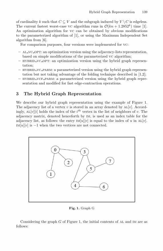
We describe our hybrid graph representation using the example of Figure 1.The adjacency list of a vertex v is stored in an array denoted by al[v]. Accord-ingly, al[v][i] holds the index of the ith vertex in the list of neighbors of v. Theadjacency matrix, denoted henceforth by im, is used as an index table for theadjacency list, as follows: the entry im[u][v] is equal to the index of u in al[v].im[u][v] is −1 when the two vertices are not connected.

Fig. 1. Graph G

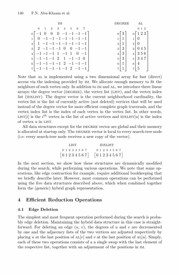
Considering the graph G of Figure 1, the initial contents of al and im are asfollows:

140 F.N. Abu-Khzam et al.

im degree al

⎡⎢⎢⎢⎢⎢⎢⎢⎢⎢⎢⎣

0 1 2 3 4 5 6 7

0 −1 0 0 0 −1 −1 −1 −11 0 −1 −1 −1 −1 −1 −1 −12 1 −1 −1 −1 −1 −1 −1 −13 2 −1 −1 −1 0 0 −1 −14 −1 −1 −1 1 −1 1 0 −15 −1 −1 −1 2 1 −1 −1 06 −1 −1 −1 −1 2 −1 −1 −17 −1 −1 −1 −1 −1 2 −1 −1

⎤⎥⎥⎥⎥⎥⎥⎥⎥⎥⎥⎦

⎡⎢⎢⎢⎢⎢⎢⎢⎢⎢⎢⎣

0 31 12 13 34 35 36 17 1

⎤⎥⎥⎥⎥⎥⎥⎥⎥⎥⎥⎦

⎡⎢⎢⎢⎢⎢⎢⎢⎢⎢⎢⎣

0 1 2

0 1 2 31 02 03 0 4 54 3 5 65 3 4 76 47 5

⎤⎥⎥⎥⎥⎥⎥⎥⎥⎥⎥⎦

Note that al is implemented using a two dimensional array for fast (direct)access via the indexing provided by im. We allocate enough memory to fit theneighbors of each vertex only. In addition to im and al, we introduce three lineararrays: the degree vector (degree), the vertex list (list), and the vertex indexlist (idxlist). The degree vector is the current neighborhood cardinality, thevertex list is the list of currently active (not deleted) vertices that will be usedinstead of the degree vector for more efficient complete graph traversals, and thevertex index list is the index of each vertex in the vertex list. In other words,list[i] is the ith vertex in the list of active vertices and idxlist[u] is the indexof vertex u in list.

All data structures except for the degree vector are global and their memoryis allocated at startup only. The degree vector is local to every search-tree node(i.e: every search-tree node receives a new copy of the vector).

list idxlist

[ 0 1 2 3 4 5 6 7

0 1 2 3 4 5 6 7] [ 0 1 2 3 4 5 6 7

0 1 2 3 4 5 6 7]

In the next section, we show how these structures are dynamically modifiedduring the search, while performing various operations. We note that some op-erations, like edge contraction for example, require additional bookkeeping thatwe briefly describe later. However, most common operations can be performedusing the five data structures described above, which when combined togetherform the (generic) hybrid graph representation.

4 Efficient Reduction Operations

4.1 Edge Deletion

The simplest and most frequent operation performed during the search is proba-bly edge deletion. Maintaining the hybrid data structure in this case is straight-forward. For deleting an edge (u, v), the degrees of u and v are decrementedby one and the adjacency lists of the two vertices are adjusted respectively byplacing u at the last position of al[v] and v at the last position of al[u]. Simply,each of these two operations consists of a a single swap with the last element ofthe respective list, together with an adjustment of the positions in im.

Hybrid Graph Representation 141

The delete edge function

Input: Edge (u,v).Begin

int i, j, x;i = im[v][u];j = −−degree[u];x = al[u][j];al[u][i] = x;al[u][j] = v;im[x][u] = i;im[v][u] = j;Repeat the previous steps for i = im[u][v] and j = −−degree[v];

End

Going back to our illustrative graph G, after deleting edge (0, 3), the modifiedal, im, and degree will look as follows (changes in bold):

im degree al

⎡⎢⎢⎢⎢⎢⎢⎢⎢⎢⎢⎣

0 1 2 3 4 5 6 7

0 −1 0 0 2 −1 −1 −1 −11 0 −1 −1 −1 −1 −1 −1 −12 1 −1 −1 −1 −1 −1 −1 −13 2 −1 −1 −1 0 0 −1 −14 −1 −1 −1 1 −1 1 0 −15 −1 −1 −1 0 1 −1 −1 06 −1 −1 −1 −1 2 −1 −1 −17 −1 −1 −1 −1 −1 2 −1 −1

⎤⎥⎥⎥⎥⎥⎥⎥⎥⎥⎥⎦

⎡⎢⎢⎢⎢⎢⎢⎢⎢⎢⎢⎣

0 21 12 13 24 35 36 17 1

⎤⎥⎥⎥⎥⎥⎥⎥⎥⎥⎥⎦

⎡⎢⎢⎢⎢⎢⎢⎢⎢⎢⎢⎣

0 1 2

0 1 2 31 02 03 5 4 04 3 5 65 3 4 76 47 5

⎤⎥⎥⎥⎥⎥⎥⎥⎥⎥⎥⎦

Notice that edge deletion runs inO(1) since all the information required for switch-ing positions in al can be found in im. Now assume we want to undo this opera-tion. This can be accomplished by simply setting degree[0] = degree[3] = 3.The only difference between this state and the initial state is that the positionsof the neighbors have changed in the adjacency lists. Knowing that every search-tree node will maintain its own copy of the degree vector, no actions whatsoeverneed to be taken to undo this operation, thus we have an “implicit-undo” for edgedeletion operations.

Remark 1. Checking if two vertices u and v are adjacent still takes constant timebut requires one additional checking: u and v are adjacent when −1 < im[u][v] <degree[v].

4.2 Vertex Deletion

Deleting a vertex v runs in Ω(d) time where d is the (current) degree of v. We runthe edge deletion operation for every active neighbor of v. In addition, we remove

142 F.N. Abu-Khzam et al.

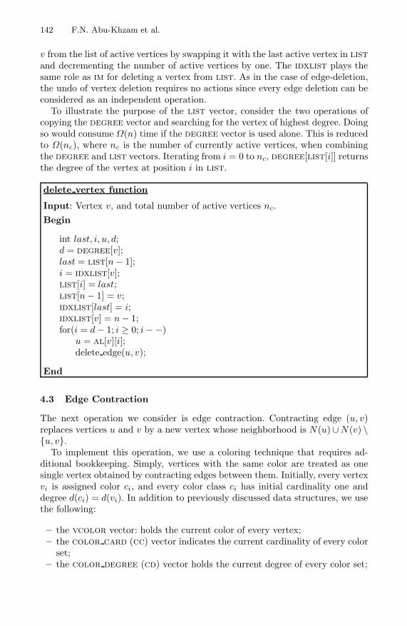
v from the list of active vertices by swapping it with the last active vertex in listand decrementing the number of active vertices by one. The idxlist plays thesame role as im for deleting a vertex from list. As in the case of edge-deletion,the undo of vertex deletion requires no actions since every edge deletion can beconsidered as an independent operation.

To illustrate the purpose of the list vector, consider the two operations ofcopying the degree vector and searching for the vertex of highest degree. Doingso would consume Ω(n) time if the degree vector is used alone. This is reducedto Ω(nc), where nc is the number of currently active vertices, when combiningthe degree and list vectors. Iterating from i = 0 to nc, degree[list[i]] returnsthe degree of the vertex at position i in list.

delete vertex function

Input: Vertex v, and total number of active vertices nc.Begin

int last, i, u, d;d = degree[v];last = list[n − 1];i = idxlist[v];list[i] = last;list[n − 1] = v;idxlist[last] = i;idxlist[v] = n − 1;for(i = d − 1; i ≥ 0; i −−)

u = al[v][i];delete edge(u, v);

End

4.3 Edge Contraction

The next operation we consider is edge contraction. Contracting edge (u, v)replaces vertices u and v by a new vertex whose neighborhood is N(u)∪N(v) \{u, v}.

To implement this operation, we use a coloring technique that requires ad-ditional bookkeeping. Simply, vertices with the same color are treated as onesingle vertex obtained by contracting edges between them. Initially, every vertexvi is assigned color ci, and every color class ci has initial cardinality one anddegree d(ci) = d(vi). In addition to previously discussed data structures, we usethe following:

– the vcolor vector: holds the current color of every vertex;– the color card (cc) vector indicates the current cardinality of every color

set;– the color degree (cd) vector holds the current degree of every color set;

Hybrid Graph Representation 143

– the color set list (csl) holds the list of vertices belonging to every colorset.

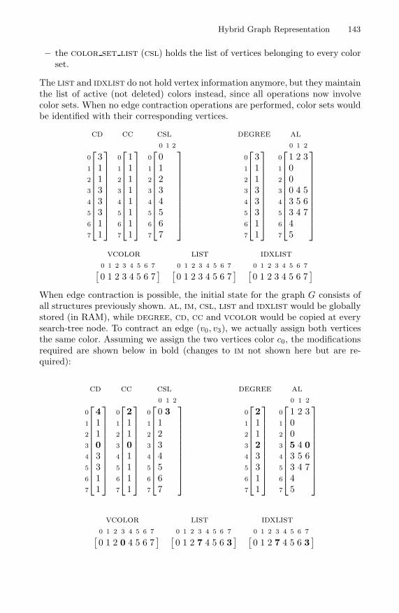
The list and idxlist do not hold vertex information anymore, but they maintainthe list of active (not deleted) colors instead, since all operations now involvecolor sets. When no edge contraction operations are performed, color sets wouldbe identified with their corresponding vertices.

cd cc csl degree al

⎡⎢⎢⎢⎢⎢⎢⎢⎢⎢⎢⎣

0 31 12 13 34 35 36 17 1

⎤⎥⎥⎥⎥⎥⎥⎥⎥⎥⎥⎦

⎡⎢⎢⎢⎢⎢⎢⎢⎢⎢⎢⎣

0 11 12 13 14 15 16 17 1

⎤⎥⎥⎥⎥⎥⎥⎥⎥⎥⎥⎦

⎡⎢⎢⎢⎢⎢⎢⎢⎢⎢⎢⎣

0 1 2

0 01 12 23 34 45 56 67 7

⎤⎥⎥⎥⎥⎥⎥⎥⎥⎥⎥⎦

⎡⎢⎢⎢⎢⎢⎢⎢⎢⎢⎢⎣

0 31 12 13 34 35 36 17 1

⎤⎥⎥⎥⎥⎥⎥⎥⎥⎥⎥⎦

⎡⎢⎢⎢⎢⎢⎢⎢⎢⎢⎢⎣

0 1 2

0 1 2 31 02 03 0 4 54 3 5 65 3 4 76 47 5

⎤⎥⎥⎥⎥⎥⎥⎥⎥⎥⎥⎦

vcolor list idxlist

[ 0 1 2 3 4 5 6 7

0 1 2 3 4 5 6 7] [ 0 1 2 3 4 5 6 7

0 1 2 3 4 5 6 7] [ 0 1 2 3 4 5 6 7

0 1 2 3 4 5 6 7]

When edge contraction is possible, the initial state for the graph G consists ofall structures previously shown. al, im, csl, list and idxlist would be globallystored (in RAM), while degree, cd, cc and vcolor would be copied at everysearch-tree node. To contract an edge (v0, v3), we actually assign both verticesthe same color. Assuming we assign the two vertices color c0, the modificationsrequired are shown below in bold (changes to im not shown here but are re-quired):

cd cc csl degree al

⎡⎢⎢⎢⎢⎢⎢⎢⎢⎢⎢⎣

0 41 12 13 04 35 36 17 1

⎤⎥⎥⎥⎥⎥⎥⎥⎥⎥⎥⎦

⎡⎢⎢⎢⎢⎢⎢⎢⎢⎢⎢⎣

0 21 12 13 04 15 16 17 1

⎤⎥⎥⎥⎥⎥⎥⎥⎥⎥⎥⎦

⎡⎢⎢⎢⎢⎢⎢⎢⎢⎢⎢⎣

0 1 2

0 0 31 12 23 34 45 56 67 7

⎤⎥⎥⎥⎥⎥⎥⎥⎥⎥⎥⎦

⎡⎢⎢⎢⎢⎢⎢⎢⎢⎢⎢⎣

0 21 12 13 24 35 36 17 1

⎤⎥⎥⎥⎥⎥⎥⎥⎥⎥⎥⎦

⎡⎢⎢⎢⎢⎢⎢⎢⎢⎢⎢⎣

0 1 2

0 1 2 31 02 03 5 4 04 3 5 65 3 4 76 47 5

⎤⎥⎥⎥⎥⎥⎥⎥⎥⎥⎥⎦

vcolor list idxlist

[ 0 1 2 3 4 5 6 7

0 1 2 0 4 5 6 7] [ 0 1 2 3 4 5 6 7

0 1 2 7 4 5 6 3] [ 0 1 2 3 4 5 6 7

0 1 2 7 4 5 6 3]

144 F.N. Abu-Khzam et al.

Since we are dealing with simple graphs, any edge between two vertices belongingto the same color set is deleted and no more than one edge is allowed between acolor set and another. Clearly, such an operation can be implicitly taken back,but is also more time and space consuming than simple vertex deletion.

This technique makes it possible to implement the vertex folding operation,introduced in [1], for the parameterized vc algorithm.

4.4 The Vertex Cover Folding Operation

Let (G, k) be an instance of the Vertex Cover problem and let u ∈ V (G) be adegree-two vertex with neighbors v and w. If v and w are adjacent, then thereis a minimum vertex cover that contains v and w (and not u). So it is safe todelete u, add v and w to the potential solution and decrement k by two. Inthe case where v and w are non-adjacent, an equivalent Vertex Cover instanceis obtained by contracting edges uv and uw and decrementing k by one. Thislatter operation is known as degree-two vertex folding.

As we shall see, applying the coloring technique to implement vertex foldingconsiderably improves the runtime on certain recalcitrant instances, but slowsdown the computation on graphs where folding rarely occurs. In such cases, theoverhead of maintaining color-sets is a drawback. Note that folding alone madeit possible to obtain a worst-case run time of O∗(1.285k) in [1]. Yet, our resultsshow that excluding folding from the same algorithm is faster on a large numberof instances, especially real ones.

5 Experimental Results

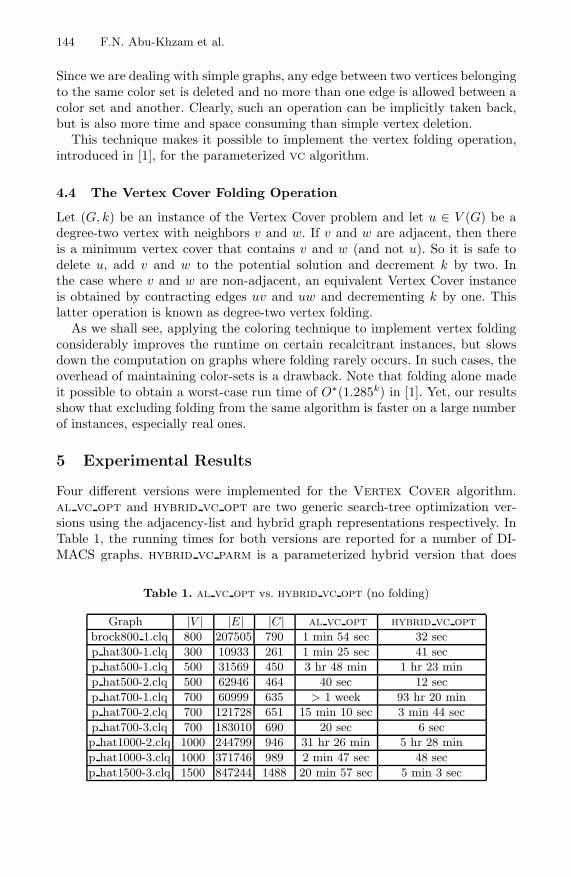
Four different versions were implemented for the Vertex Cover algorithm.al vc opt and hybrid vc opt are two generic search-tree optimization ver-sions using the adjacency-list and hybrid graph representations respectively. InTable 1, the running times for both versions are reported for a number of DI-MACS graphs. hybrid vc parm is a parameterized hybrid version that does

Table 1. al vc opt vs. hybrid vc opt (no folding)

Graph |V | |E| |C| al vc opt hybrid vc opt

brock800 1.clq 800 207505 790 1 min 54 sec 32 sec

p hat300-1.clq 300 10933 261 1 min 25 sec 41 sec

p hat500-1.clq 500 31569 450 3 hr 48 min 1 hr 23 min

p hat500-2.clq 500 62946 464 40 sec 12 sec

p hat700-1.clq 700 60999 635 > 1 week 93 hr 20 min

p hat700-2.clq 700 121728 651 15 min 10 sec 3 min 44 sec

p hat700-3.clq 700 183010 690 20 sec 6 sec

p hat1000-2.clq 1000 244799 946 31 hr 26 min 5 hr 28 min

p hat1000-3.clq 1000 371746 989 2 min 47 sec 48 sec

p hat1500-3.clq 1500 847244 1488 20 min 57 sec 5 min 3 sec

Hybrid Graph Representation 145

Table 2. hybrid vc parm vs. hybrid vcf parm (with folding) on a 4-regular graphhaving 300 vertices and 600 edges

Vertex Cover Size (|K|) Answer No Folding With Folding

192 yes 14 sec < 1 sec

191 yes 17 sec 6 sec

190 yes 2 hr 14 min 6 min 27 sec

165 no > 4 days 46 min 56 sec

160 no 38 hr 2 min 2 min 32 sec

Table 3. al ds opt vs. hybrid ds opt

Graph |V | |E| |D| al ds opt hybrid ds opt

rgraph1 100 400 16 21 min 4 sec 4 min 11 sec

rgraph2 100 600 11 5 min 5 sec 53 sec

rgraph3 100 1500 6 41 sec 5 sec

rgraph4 150 1200 14 16 hr 46 min 2 hr 27 min

rgraph5 150 1500 11 3 hr 31 min 28 min 20 sec

rgraph6 150 3000 6 2 min 8 sec 12 sec

rgraph7 150 3000 7 27 min 16 sec 2 min 1 sec

rgraph8 200 4500 9 5 hr 44 min 30 min 8 sec

rgraph9 200 5000 8 1 hr 20 min 6 min 46 sec

rgraph10 200 6000 6 1 hr 36 min 7 min 13 sec

rgraph11 200 12000 4 6 min 49 sec 17 sec

rgraph12 250 9000 8 14 hr 37 min 56 min 53 sec

rgraph13 250 10000 7 1 hr 30 min 5 min 34 sec

rgraph14 250 12000 5 4 hr 41 min 16 min 19 sec

rgraph15 250 24000 3 19 sec < 1 sec

rgraph16 300 22461 4 8 min 31 sec 17 sec

rgraph17 300 22258 4 28 min 32 sec 1 min 10 sec

rgraph18 300 11063 8 133 hr 38 min 5 hr 54 min

rgraph19 300 11287 8 > 7 days 8 hr 14 min

rgraph20 1000 374633 3 4 min 37 sec 2 min 29 sec

rgraph21 1000 374552 3 28 min 37 sec 6 min 36 sec

not take advantage of vertex folding, while hybrid vcf parm is a parameter-ized version implemented using the coloring technique described in the previoussection for folding.

In general, the folding technique is at most two times slower than the simplegeneric branching algorithm. It gets faster as the difference between the highestand lowest vertex-degrees gets smaller. In particular, applying vertex folding,via our coloring technique, is much faster on regular graphs. To illustrate, testswere run on a 4-regular graph, by varying the input parameter, and results arereported in Table 2.

As for the Dominating Set problem, al ds opt denotes the optimiza-tion version using the adjacency-lists representation and hybrid ds opt the

146 F.N. Abu-Khzam et al.

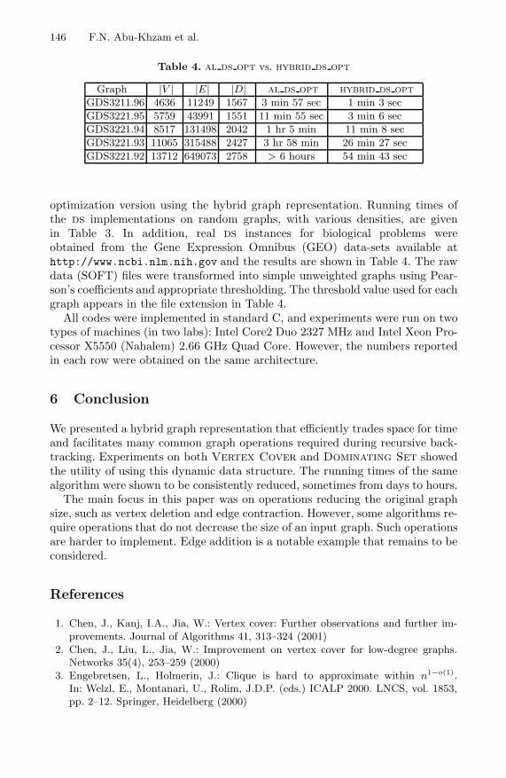
Table 4. al ds opt vs. hybrid ds opt

Graph |V | |E| |D| al ds opt hybrid ds opt

GDS3211.96 4636 11249 1567 3 min 57 sec 1 min 3 sec

GDS3221.95 5759 43991 1551 11 min 55 sec 3 min 6 sec

GDS3221.94 8517 131498 2042 1 hr 5 min 11 min 8 sec

GDS3221.93 11065 315488 2427 3 hr 58 min 26 min 27 sec

GDS3221.92 13712 649073 2758 > 6 hours 54 min 43 sec

optimization version using the hybrid graph representation. Running times ofthe ds implementations on random graphs, with various densities, are givenin Table 3. In addition, real ds instances for biological problems wereobtained from the Gene Expression Omnibus (GEO) data-sets available athttp://www.ncbi.nlm.nih.gov and the results are shown in Table 4. The rawdata (SOFT) files were transformed into simple unweighted graphs using Pear-son’s coefficients and appropriate thresholding. The threshold value used for eachgraph appears in the file extension in Table 4.

All codes were implemented in standard C, and experiments were run on twotypes of machines (in two labs): Intel Core2 Duo 2327 MHz and Intel Xeon Pro-cessor X5550 (Nahalem) 2.66 GHz Quad Core. However, the numbers reportedin each row were obtained on the same architecture.

6 Conclusion

We presented a hybrid graph representation that efficiently trades space for timeand facilitates many common graph operations required during recursive back-tracking. Experiments on both Vertex Cover and Dominating Set showedthe utility of using this dynamic data structure. The running times of the samealgorithm were shown to be consistently reduced, sometimes from days to hours.

The main focus in this paper was on operations reducing the original graphsize, such as vertex deletion and edge contraction. However, some algorithms re-quire operations that do not decrease the size of an input graph. Such operationsare harder to implement. Edge addition is a notable example that remains to beconsidered.

References

1. Chen, J., Kanj, I.A., Jia, W.: Vertex cover: Further observations and further im-provements. Journal of Algorithms 41, 313–324 (2001)

2. Chen, J., Liu, L., Jia, W.: Improvement on vertex cover for low-degree graphs.Networks 35(4), 253–259 (2000)

3. Engebretsen, L., Holmerin, J.: Clique is hard to approximate within n1−o(1).In: Welzl, E., Montanari, U., Rolim, J.D.P. (eds.) ICALP 2000. LNCS, vol. 1853,pp. 2–12. Springer, Heidelberg (2000)

Hybrid Graph Representation 147

4. Fomin, F.V., Grandoni, F., Kratsch, D.: Measure and conquer: domination - a casestudy. In: Caires, L., Italiano, G.F., Monteiro, L., Palamidessi, C., Yung, M. (eds.)ICALP 2005. LNCS, vol. 3580, pp. 191–203. Springer, Heidelberg (2005)

5. Fomin, F.V., Grandoni, F., Kratsch, D.: Solving connected dominating set fasterthan 2n. Algorithmica 52(2), 153–166 (2008)

6. Fomin, F.V., Grandoni, F., Kratsch, D.: Measure and conquer: a simple O(20.288n)independent set algorithm. In: Proceedings of the seventeenth annual ACM-SIAMsymposium on Discrete algorithm (SODA), New York, USA, pp. 18–25 (2006)

7. Fomin, F.V., Kratsch, D., Woeginger, L., Woeginger, G.J.: Exact (exponential) al-gorithms for the dominating set problem. In: Hromkovic, J., Nagl, M., Westfechtel,B. (eds.) WG 2004. LNCS, vol. 3353, pp. 245–256. Springer, Heidelberg (2004)

8. Grandoni, F.: A note on the complexity of minimum dominating set. J. DiscreteAlgorithms 4(2), 209–214 (2006)

9. Hastad, J.: Clique is hard to approximate within n(1−ε). Acta Mathematica,627–636 (1996)

10. Randerath, B., Schiermeyer, I.: Exact algorithms for minimum dominating set.Technical report, Zentrum fur Angewandte Informatik Koln, Lehrstuhl Specken-meyer (2004)

11. van Rooij, J.M., Bodlaender, H.L.: Exact algorithms for edge domination. Techni-cal Report UU-CS-2007-051, Department of Information and Computing Sciences,Utrecht University (2007)

12. van Rooij, J.M., Nederlof, J., van Dijk, T.C.: Inclusion/exclusion meets measureand conquer: Exact algorithms for counting dominating sets. Technical ReportUU-CS-2008-043, Department of Information and Computing Sciences, UtrechtUniversity (2008)

13. van Rooij, J.M., Bodlaender, H.L.: Design by measure and conquer, a faster exactalgorithm for dominating set. In: Albers, S., Weil, P. (eds.) STACS. LIPIcs, vol. 1,pp. 657–668. Schloss Dagstuhl - Leibniz-Zentrum fuer Informatik, Germany (2008)