P OLITECNICO DI MILANO DIPARTIMENTO DI ELETTRONICA,I NFORMAZIONE E BIOINGEGNERIA DOCTORAL P ROGRAMME I N I NFORMATION TECHNOLOGY A HOLISTIC APPROACH TOWARDS FUTURE SELF - TUNING APPLICATIONS IN HOMOGENEOUS AND HETEROGENEOUS ARCHITECTURES Doctoral Dissertation of: Emanuele Vitali Supervisor: Prof. Gianluca Palermo Tutor: Prof. Cristina Silvano The Chair of the Doctoral Program: Prof. Barbara Pernici Year 2021 – Cycle XXXII

Welcome message from author
This document is posted to help you gain knowledge. Please leave a comment to let me know what you think about it! Share it to your friends and learn new things together.
Transcript
POLITECNICO DI MILANODIPARTIMENTO DI ELETTRONICA, INFORMAZIONE E BIOINGEGNERIA
DOCTORAL PROGRAMME IN INFORMATION TECHNOLOGY
A HOLISTIC APPROACH TOWARDS FUTURE
SELF-TUNING APPLICATIONS IN HOMOGENEOUS
AND HETEROGENEOUS ARCHITECTURES
Doctoral Dissertation of:Emanuele Vitali
Supervisor:Prof. Gianluca Palermo
Tutor:Prof. Cristina Silvano
The Chair of the Doctoral Program:Prof. Barbara Pernici
Year 2021 – Cycle XXXII

Abstract
WITH the beginning of the dark silicon era, application optimiza-tion, even with the exploitation of heterogeneity, has becomean important topic of research. One methodology to obtain op-
timized applications for different architectures is application autotuning.Indeed, applications can obtain the same result with different codes. How-ever, different codes have different extra-functional properties, such as ex-ecution time or energy consumption which may change across differentarchitectures. To obtain the best, application autotuning techniques havebeen proposed in literature. It is very difficult for the original applicationdeveloper to select the best configuration that can enforce the constraintsacross different machines, with unknown input and varying configurations.
Given this background, I envision future applications not as monolithiccode but as a sequence of modules that are capable of autotuning them-selves and can exploit platform heterogeneity. This thesis consists of acollection of methodologies that were developed during my Ph.D. whichaim at giving the programmers ways to create these self-tuning modules.
I divided my Ph.D. thesis into two sections, the first one is dedicatedto general application autotuning techniques, while the second will be fo-cused on a single application, GeoDock, which has been an industrial usecase that I used to develop and validate the proposed techniques. In the firsthalf, we will see the benefit that can be introduced by run-time dynamicautotuning focusing on the condition of the machine, constraints given tothe application, or characteristics of the input data. In the second half, wewill see the developement of GeoDock from a monolithic non tunable ap-
I

plication to an heterogeneous and tunable one, and we will see how this hasdramatically improved its performances (from tens of ligands per secondprocessed on a single node to thousands).
II
Contents
1 Introduction 11.1 Thesis Motivations . . . . . . . . . . . . . . . . . . . . . . 21.2 Thesis Contributions . . . . . . . . . . . . . . . . . . . . . 31.3 Thesis Outline . . . . . . . . . . . . . . . . . . . . . . . . 4
2 Previous work 92.1 Background and definitions . . . . . . . . . . . . . . . . . . 92.2 Autotuning . . . . . . . . . . . . . . . . . . . . . . . . . . 11
2.2.1 Autotuning Time Strategies . . . . . . . . . . . . . . 112.2.2 Autotuning Integration Strategies . . . . . . . . . . . 12
2.3 mARGOt . . . . . . . . . . . . . . . . . . . . . . . . . . . 192.3.1 Application-knowledge . . . . . . . . . . . . . . . . 212.3.2 Monitors . . . . . . . . . . . . . . . . . . . . . . . . 222.3.3 Application Manager . . . . . . . . . . . . . . . . . 222.3.4 Integration Effort . . . . . . . . . . . . . . . . . . . 24
2.4 Summary . . . . . . . . . . . . . . . . . . . . . . . . . . . 25
3 Methodology 27
I General Autotuning Techniques 31
4 A Seamless Online Compiler and System Runtime Autotuning Frame-work 334.1 Introduction . . . . . . . . . . . . . . . . . . . . . . . . . . 33
III
Contents
4.2 Background . . . . . . . . . . . . . . . . . . . . . . . . . . 354.3 Proposed Methodology . . . . . . . . . . . . . . . . . . . . 36
4.3.1 Step 1: Reduce the compiler flag space . . . . . . . . 384.3.2 Step 2: Integration . . . . . . . . . . . . . . . . . . . 38
4.4 Experimental Results . . . . . . . . . . . . . . . . . . . . . 404.5 Summary . . . . . . . . . . . . . . . . . . . . . . . . . . . 44
5 A library for tunable Multipliers Hardware Accelerators 455.1 Introduction . . . . . . . . . . . . . . . . . . . . . . . . . . 465.2 Background . . . . . . . . . . . . . . . . . . . . . . . . . . 485.3 Target Class of Multiplication Algorithms . . . . . . . . . . 495.4 The Proposed Approach . . . . . . . . . . . . . . . . . . . 515.5 Experimental Results . . . . . . . . . . . . . . . . . . . . . 565.6 Summary . . . . . . . . . . . . . . . . . . . . . . . . . . . 60
6 Autotuning a Server-Side Car Navigation System 616.1 Introduction . . . . . . . . . . . . . . . . . . . . . . . . . . 626.2 Background . . . . . . . . . . . . . . . . . . . . . . . . . . 646.3 Monte Carlo Approach for Probabilistic Time-Dependent Rout-
ing . . . . . . . . . . . . . . . . . . . . . . . . . . . . . . . 666.4 The Proposed Approach . . . . . . . . . . . . . . . . . . . 69
6.4.1 Unpredictability Feature . . . . . . . . . . . . . . . . 726.4.2 Error Prediction Function . . . . . . . . . . . . . . . 73
6.5 Integration Flow . . . . . . . . . . . . . . . . . . . . . . . 746.6 Experimental Results . . . . . . . . . . . . . . . . . . . . . 79
6.6.1 Training the Model . . . . . . . . . . . . . . . . . . 796.6.2 Validation Results . . . . . . . . . . . . . . . . . . . 816.6.3 Comparative Results with Static Approach . . . . . . 836.6.4 Overhead Analysis . . . . . . . . . . . . . . . . . . . 876.6.5 System-Level Performance Evaluation . . . . . . . . 88
6.7 Summary . . . . . . . . . . . . . . . . . . . . . . . . . . . 89
7 Demonstrating the benefit of Autotuning in Object Detection context 917.1 Introduction . . . . . . . . . . . . . . . . . . . . . . . . . . 927.2 Background . . . . . . . . . . . . . . . . . . . . . . . . . . 947.3 Motivations . . . . . . . . . . . . . . . . . . . . . . . . . . 947.4 The Proposed Approach . . . . . . . . . . . . . . . . . . . 98
7.4.1 Reactive approach . . . . . . . . . . . . . . . . . . . 997.4.2 Proactive approach . . . . . . . . . . . . . . . . . . . 101
7.5 Summary . . . . . . . . . . . . . . . . . . . . . . . . . . . 106
IV
Contents
II Geometric Docking case studies 107
8 Background 109
9 Introducing Autotuning in GeoDock in a Homogeneous Context 1139.1 Introduction . . . . . . . . . . . . . . . . . . . . . . . . . . 1139.2 Background . . . . . . . . . . . . . . . . . . . . . . . . . . 1159.3 Methodology . . . . . . . . . . . . . . . . . . . . . . . . . 116
9.3.1 Application Description . . . . . . . . . . . . . . . . 1169.3.2 Analysis of Geodock . . . . . . . . . . . . . . . . . 1179.3.3 Exposing Tunable Application Knobs . . . . . . . . . 1239.3.4 Application Autotuning . . . . . . . . . . . . . . . . 125
9.4 Experimental Setup . . . . . . . . . . . . . . . . . . . . . . 1289.4.1 Data Sets . . . . . . . . . . . . . . . . . . . . . . . . 1289.4.2 Metrics of Interest . . . . . . . . . . . . . . . . . . . 1289.4.3 Target Platform . . . . . . . . . . . . . . . . . . . . 129
9.5 Experimental Results . . . . . . . . . . . . . . . . . . . . . 1299.5.1 Data Dependency Evaluation . . . . . . . . . . . . . 1299.5.2 Trade-off Analysis . . . . . . . . . . . . . . . . . . . 1319.5.3 Time-to-solution Model Validation . . . . . . . . . . 1339.5.4 Use-case Scenarios . . . . . . . . . . . . . . . . . . 134
9.6 Summary . . . . . . . . . . . . . . . . . . . . . . . . . . . 137
10 Porting and Tuning Geodock kernels to GPU using OpenACC 13910.1 Introduction . . . . . . . . . . . . . . . . . . . . . . . . . . 13910.2 Background . . . . . . . . . . . . . . . . . . . . . . . . . . 14110.3 The Proposed Approach . . . . . . . . . . . . . . . . . . . 142
10.3.1 Application Description . . . . . . . . . . . . . . . . 14210.3.2 Profiling . . . . . . . . . . . . . . . . . . . . . . . . 14410.3.3 Implementation . . . . . . . . . . . . . . . . . . . . 145
10.4 Experimental Results . . . . . . . . . . . . . . . . . . . . . 14810.4.1 Performance evaluation on the GPU . . . . . . . . . 14810.4.2 Performance comparison with baseline . . . . . . . . 15010.4.3 Performance evaluation on the CPU . . . . . . . . . . 152
10.5 Summary . . . . . . . . . . . . . . . . . . . . . . . . . . . 153
11 Optimizing GeoDock Throughput in Heterogeneous Platforms 15511.1 Introduction . . . . . . . . . . . . . . . . . . . . . . . . . . 15611.2 Background . . . . . . . . . . . . . . . . . . . . . . . . . . 15711.3 The Proposed Approach . . . . . . . . . . . . . . . . . . . 158
11.3.1 OpenACC Implementation . . . . . . . . . . . . . . 159
V
Contents
11.3.2 Hybrid OpenMP/OpenACC Implementation . . . . . 16111.4 Experimental Results . . . . . . . . . . . . . . . . . . . . . 167
11.4.1 Single GPU . . . . . . . . . . . . . . . . . . . . . . 16811.4.2 Multi-GPUs . . . . . . . . . . . . . . . . . . . . . . 170
11.5 Summary . . . . . . . . . . . . . . . . . . . . . . . . . . . 174
12 Improving GeoDock GPU efficiency with Cuda and Dynamic KernelTuning 17512.1 Introduction . . . . . . . . . . . . . . . . . . . . . . . . . . 17612.2 Background . . . . . . . . . . . . . . . . . . . . . . . . . . 17712.3 Porting to CUDA . . . . . . . . . . . . . . . . . . . . . . . 178
12.3.1 General Considerations . . . . . . . . . . . . . . . . 17812.3.2 Kernels analysis and optimizations . . . . . . . . . . 181
12.4 Experimental Results . . . . . . . . . . . . . . . . . . . . . 19012.5 Autotuning . . . . . . . . . . . . . . . . . . . . . . . . . . 19212.6 Summary . . . . . . . . . . . . . . . . . . . . . . . . . . . 194
13 Conclusions 19713.1 Main contributions . . . . . . . . . . . . . . . . . . . . . . 19713.2 Recommendation for future works . . . . . . . . . . . . . . 199
Publications 201
Bibliography 205
VI
CHAPTER1Introduction
With the end of Dennard scaling and the beginning of the Dark Siliconera [1], power consumption has become the limit of modern systems. Mul-ticore processors have been the first answer to the end of Dennard scaling,however dark silicon limits even this approach. For this reason, in the latestyears, heterogeneous architectures have become always more widespread,thanks to their lower cost of FLOPs per watt [2].
This shift of paradigm introduces a change in application development,since writing code while targeting heterogeneity is more difficult. The pro-grammer needs to consider more details when designing the application,such as data movement between processor and co-processor. Moreover, ithas become fundamental to consider extra-functional properties (EFP) suchas energy efficiency or time-to-solution. In particular energy efficiency,which was a property mainly related to embedded systems, is now con-sidered fundamental in a wider range of contexts up to High-PerformanceComputing (HPC).
Among all the possibilities, this thesis focuses on two software aspects.The first aspect is Application Parameterization. When writing an appli-cation, it is possible to obtain the same result with different EFPs. It isgood practice for programmers to expose some implementation parameters
1
Chapter 1. Introduction
whenever they may alter EFP without altering the behavior of the code.Examples of these parameters may be the number of worker threads, or thealgorithm used for a specific operation (e.g. the sorting algorithm). An-other possible parameter is the hardware used for the execution of a func-tion. These parameters in literature are called software knobs if they can bemodified only at compile time. If they can be modified at run-time, they arecalled dynamic knobs.
The second aspect is Approximate Computing. In this approach, theobjective of an application is to compute a result that is good enough forthe user and not the exact one [3]. This allows avoiding some computation,which means energy, to obtain the result. This approach is commonly usedto expose accuracy-throughput software knobs. It is common in multimediaapplications or where is possible to use techniques such as task skipping [4]or loop perforation [5]. It has been shown in literature [6] that this techniquecan exchange the accuracy of the result for throughput. For this reason,approximate hardware has also been explored [7, 8].
Given all these aspects, optimizing applications across different systemsis becoming a complex task. Indeed, the tradeoffs exposed by approxi-mate computing or by the software knobs make applications difficult to setup for the end-user. Moreover, requirements might contain constraints onextra-functional properties, or some input properties can create some opti-mization opportunities.
In this context, to help developers, the autonomic computing approachhas been proposed [9], where the applications are enhanced with a set ofself-* properties, such as self-healing, self-optimization or self-protection.This thesis will focus on the self-optimization property. This property aimsat enhancing the application by enabling it to find and exploit optimizationopportunities given by the system evolution.
1.1 Thesis Motivations
With the rise of heterogeneous platforms, the already difficult task of opti-mizing an application has become even more difficult. Indeed, the amountof possibilities to tune extra-functional properties has increased, since wealso need to consider which component we are going to run the application(or even part of it) on.
In order to obtain the best, application autotuning techniques have beenproposed in literature. The importance of autotuning lies in the fact thatit is very difficult for the original application developer to select the bestconfiguration that can enforce the constraints across different machines,
2
1.2. Thesis Contributions
with unknown input and varying configurations.In this context, I want to insert the work of my thesis. I envision future
application not as monolithic code, but as a sequence of self-tuning mod-ules, capable of adapt themselves in two orthogonal directions. The first isadaptivity to the input, intended as being able to change how the applicationperforms its work according to some characteristics of the input data. Thesecond is adaptivity to the platform, intended as being capable of changingaccording to varying runtime constraints and exploit, whenever available,the heterogeneity of present and future platforms.
This thesis consists of a collection of methodologies that aim at advanc-ing the state of the art in the field of application autotuning with a focus onheterogeneity.
1.2 Thesis Contributions
The main contribution of this thesis is a collection of techniques to enhancea target application with autotuning capabilities, with a focus on hetero-geneous contexts in the second part of the thesis. As these techniques arestrongly tailored to the target application, they are not implemented in a sin-gle framework. However, the methodology behind them is general and canbe easily ported into similar contexts. Furthermore, these methodologieshave been developed inside two European Projects, ANTAREX (AutoTun-ing and Adaptivity appRoach for Energy efficient eXascale HPC systems)and E4C (Exscalate4Cov).
In particular, the contributions are the following:
1. A framework to automatically tune compiler flags or library parame-ters at function level. The framework exploits different tools (mAR-GOt [10], COBAYN [11], LARA [12], MilepostGCC [13]) in a jointeffort to ease the programmer job and automatically and seamlesslyobtain the best possible configuration according to the underlying ar-chitecture for every different hotspot kernel in the code.
2. Analysis of applications to find and expose autotuning possibilitiesin a reactive way. Applications have been made capable to react tochanges in the underlying configurations or changing requirementsprovided by the user.
3. A methodology has been developed to respect a requirement on timeto solution of an application that has been previously enriched withautotuning capabilities.
3
Chapter 1. Introduction
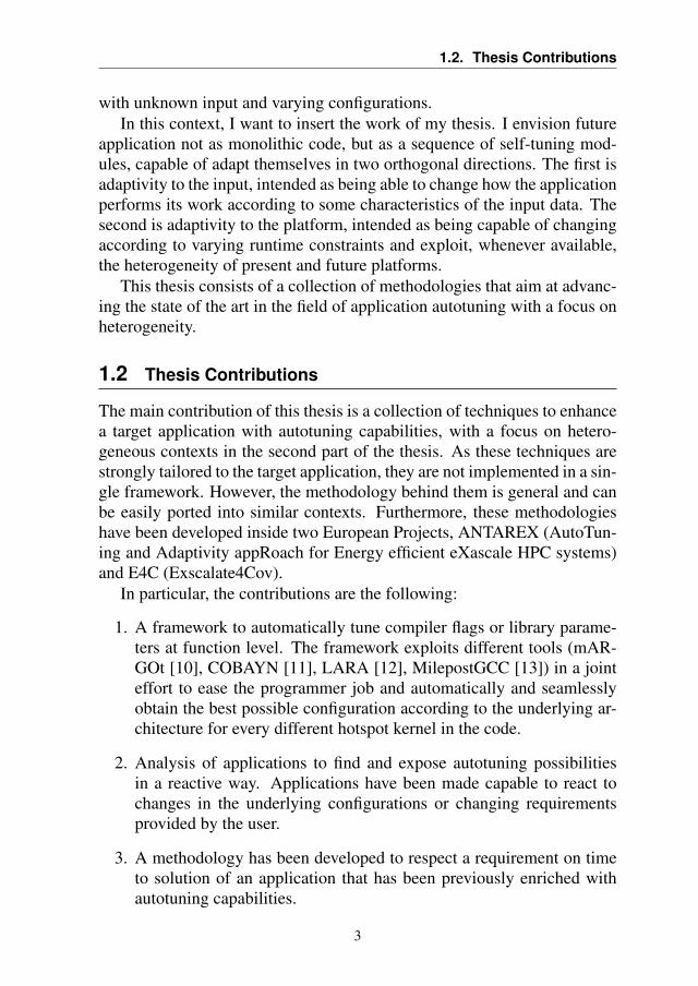
Table 1.1: Techniques developed in this thesis and application for which they were tai-lored. Global means that the technique does not have a specific application.
Technique Global GeoDock PTDR Object Detection MultiplicationFunction Level Autotuning Chapter 4
Reactive Autotuning Chapter 9 Chapter 7Time to Solution Chapter 9
Proactive Autotuning Chapter 12 Chapter 6 Chapter 7Heterogeneity Parameters Tuning Chapter 10
Hybrid approach Chapter 11Tunable Library Chapter 5
4. A methodology to proactively autotune applications according to theinput data.The objective of this methodology is to increase computa-tion efficiency and thus save energy and time.
5. Porting of an application to the heterogeneous context, using the Ope-nACC language, and optimization of its computation organization onthe GPU.
6. Optimization of the distribution of the computation across CPU andGPU, mapping the kernels on the most suitable hardware according tothe characteristics of the kernel itself.
7. Creation of a parametric library for the synthesis of long unsignedmultipliers on FPGA. The library allows the programmers to createhardware accelerators to perform this important operation with a fo-cus on parametrization and the offering of several trade-offs in perfor-mance and cost.
As previously mentioned, these methodologies have been studied in dif-ferent use cases and application. Table 1.1 reports for all the techniquespreviously described on which application they have been ported and inwhich chapter this will be discussed.
In the remainder of this thesis, I will write using the first-person plural toacknowledge the support from my advisor and colleagues. However, I takeresponsibility for all the decisions and choices described in this thesis, sinceI was the main investigator. The only exceptions are the works described,Chapter 4 and Chapter 9, which are a joint effort with other colleagues.
1.3 Thesis Outline
This thesis is organized into three main sections. The first section focuseson the state of the art in application autotuning. Firstly we describe the re-search done up to now, then a background section focuses on the mARGOtautotuner, a tool that I contributed to develop.
4
1.3. Thesis Outline
User Required code
Self-Tuning Module
Heterogeneity Space
Originalapplication
source code
Code FeatureExtraction
Compilerflags space
Compiler flags
Compiler FlagSelection
Libraries Parameter
Space
DSL seamlessintegration
Enhancedapplication
source code
Profilingbinary
Applicationknowledge
Adaptivebinary
Runtime library
Framework API
Autotuner
Profiling library
Manual Integration
Application Specific Code
Data Features
HLS Kernels
GPU Kernels
FPGA Kernel
GPU Kernel
Constraints
Manual KnobsExposition
FunctionInstrumentation
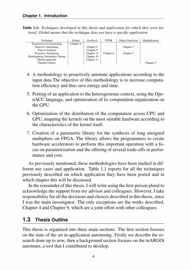
Figure 1.1: Global architecture of the proposed framework.
The second section is divided into 4 chapters, and focuses on differentmethodologies for autotuning applications, at compiler, library or applica-tion level. The third section focuses on a single application, a moleculardocking tool, that has been used as a use case several times during myPh.D. to develop and validate new techniques. In last section we will alsodescribe its evolution and we will refer to some experiments that were madepossible thanks to the introduced innovation.
Finally, Chapter 13 summarizes the proposed approach and states rec-ommendations for future works.
The work of this thesis has not been implemented in a single frameworkbut is a collection of methodologies. However, they aim at suggesting aglobal collective paradigm for writing future applications.
Figure 1.1 shows the global vision of a self-tuning module. As we cansee, a lot of different components are added to the original source code ofthe application to obtain the final adaptive binary. Not all of these compo-nents are present together in any of the analyzed scenarios, however, therehas always been a global view that has driven the work of this thesis.
5
Chapter 1. Introduction
We can clusterize the components into three different macro categories:
• Code-related tunable parameters.
• Data features.
• Heterogeneous components.
The first category comprehends all of those characteristics such as com-piler flags and library-related parameters, whose optimality may be depen-dent on the environment of the execution of the code. The autotuning ofthese parameter has been investigated in Chapter 4 and Chapter 9.
In Chapter 4 we propose a methodology to seamlessly and automati-cally select, at function level, the optimal configuration of compiler flagsand OpenMP parameters. In Chapter 9 instead, we study a particular appli-cation to find autotuning opportunities, and we propose a technique to setand enforce a time to solution on the application runtime.
The second category is related to the application data. Indeed, some ap-plications may require different behavior according to different inputs, andthe optimality of the application can change (there is no one-fits-all solu-tion). We investigated this perspective mainly in Chapter 6 and Chapter 7.
In Chapter 6 we studied a Probabilistic Time-Dependent Routing algo-rithm for a navigation application and noticed that some characteristics ofthe input, which we called Data Features, could be used to tune the Mon-teCarlo simulation to improve the computation efficiency. In Chapter 7 westudied different object detection networks and demonstrated that no so-lution is optimal for all the images. Even if we were unable to build apredictor, we believe that this work shows the potential of the autotuningparadigm in this field.
The third category is related to the exploitation of heterogeneity sincewe want our application to be able to use all the computing resources avail-able on the machine where it is running. This approach has been studiedon the GPU with the evolution of the geometric docking application (Chap-ter 10, Chapter 11 and Chapter 12 ) and on FPGA with the development ofa parametric library for unsigned long multiplication (Chapter 5).
In particular, in Chapter 10 we followed a traditional approach for GPUkernel development using the OpenACC language followed by a parame-ter space exploration and autotuning. In Chapter 11 we further optimizedthe previous work by considering hardware characteristics when selectingwhere to run the different kernels that compose the application. Finally, inChapter 12, we optimized the application for a novel GPU and we applied
6

1.3. Thesis Outline
the Data Feature approach in a heterogeneous context, showing that it canintroduce benefits.
In Chapter 5 we developed a library to create, exploiting High LevelSynthesis, hardware accelerators for the multiplication of large unsignedintegers. The library is heavily parametrized and can create acceleratorsthat cover several orders of magnitude in terms of performance and resourceutilization, according to the constraints of the programmers.
The content of most of the chapters of this thesis has already been pub-lished in international conferences or journals. The reuse of the imagesfrom those sources has been highlighted under each caption.
7

CHAPTER2Previous work
The main focus of this thesis is to develop a general approach for applica-tion autotuning in a heterogeneous system. The approach will be proposedwith several case studies, where it has been tailored to specific applications.
This chapter provides at first an introduction to the related researchfield, and it defines a common terminology in the state-of-the-art. Thenit describes the mARGOt framework, an autotuning framework that I con-tributed to develop to support the analysis carried out in this thesis.
2.1 Background and definitions
The methodology proposed by this thesis belongs to the autonomic com-puting research topic. In this field, computing systems can be called auto-nomic if they are able, thanks to a set of elements, to manage themselveswithout a human in the loop. In the original work [9], four aspects of self-management have been identified.
• Self-Configuration: the system shall be able to configure automati-cally, according to high-level policies. When a new component isintegrated, it has to seamlessly integrate into the system. An examplecan be found in [14].
9
Chapter 2. Previous work
• Self-Optimization: the system will have to seek to improve their per-formances. They have to continually monitor, experiment and tunetheir parameters.
• Self-Healing: the system has to detect and repair localized softwareand hardware problems, as proposed in [15].
• Self-Protection: the system must defend itself from attacks, as pro-posed in [16].
In this work, we will focus on Self-Optimization property. Previous surveys[17–19] can give a more detailed view on the autonomic computing fieldfor the other self-* properties.
In the autonomic computing field, a system is composed of both hard-ware and software components. Therefore, in literature, several approacheshave been proposed to optimize the efficiency of both. In particular, we candivide these approaches into two orthogonal categories:
• Resource Managers: in this category fall all the approaches wherethe Self-Optimization property is obtained through resource manage-ment or allocation. Usually, there is a task at system level that isin charge of distributing the resources across the different applica-tions. This approach is quite wide-spread and can be found in datacenters [20,21], in grid computing [22], in multicores [23–25], in em-bedded contexts [26, 27] or in heterogeneous systems [28].
• Application Autotuners: all the approaches where the Self-Optimizationproperty is obtained at software level by the application itself fall inthis category. Here the application can manage some configurationparameters to reach the end-user requirement. In this thesis, we willfocus on this approach.
Before going in-depth with the literature in the autotuning field, we needto clarify the definition of some key concepts. The first important keywordis the term application. In this work, with application we consider a sub-set of all the possible software that may run on the system. In particular,we will consider only the applications that perform an elaboration withoutany human interaction, such as a molecular docking application or a nav-igation system. Another key concept is the definition of metrics. We callmetric any measurable property of the application that can be targeted byan optimization problem, i.e. what in literature is called Extra FunctionalProperty (EFP) or Non Functional Property, such as energy consumption,time to solution, or quality of the result that the end-user can be interested
10
2.2. Autotuning
in minimizing or maximizing. Examples of metrics that we will see in thisthesis are the minimization of energy consumption, in the navigation sys-tem application, while respecting user service level agreement. Or the timeto solution of a batch molecular docking application while maximizing theoutput quality. As we already mentioned, many applications expose sometunable parameters, called Software Knobs, that can be modified to changethe EFPs of the application according to the end-user requirements. Finally,there is the concept of Input Features. It is possible in some circumstancesthat some characteristics of the input (such as its size) can help the processof self-optimization. This happens if some correlation between the inputand the metric can be found.
2.2 Autotuning
In this section, we will introduce and classify all those techniques proposedin the literature that aims at giving the Self-Optimization property.
A first classification of the autotuning techniques can be done by clus-tering them according to when autotuning happens, which means at deploytime or runtime. We define this classification as "Autotuning Time Classifi-cation" A second classification can be done according to the invasiveness ofthe autotuning technique in the original application. We define this classi-fication as "Autotuning Integration Classification". In this section, we willsee the difference between the two taxonomies and we will explore the stateof the art following the second classification strategy
2.2.1 Autotuning Time Strategies
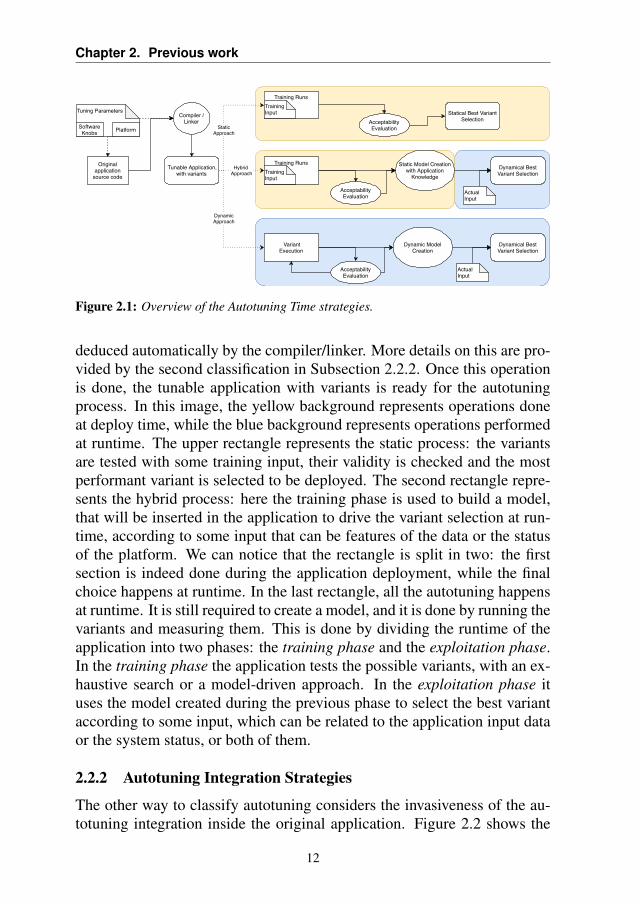
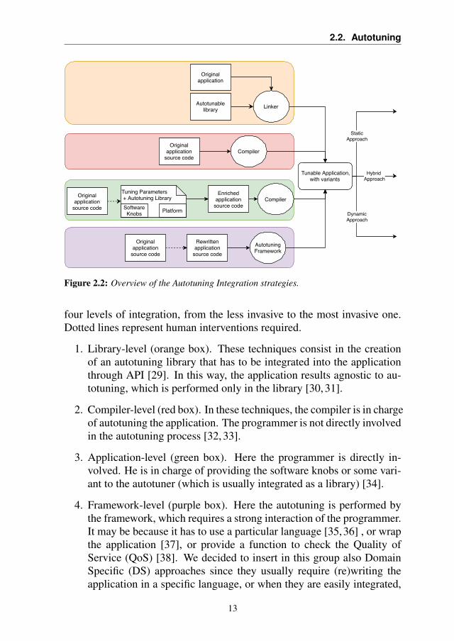
We can distinguish different autotuning approaches according to "when"the autotuning happens during the lifetime of the application. On one hand,the autotuning is performed during the software installation on the plat-form: variants are generated statically, they are tested (all or through amodel-driven approach) and the best one is selected. This approach is alsocalled static autotuning. On the other hand, the variations are generated atruntime giving more flexibility (at the cost of greater overheads). This ap-proach is also known as dynamic autotuning. Between these two extremesolutions, there is a compromise in the middle: the variants can be createdat deploy or design time, but selected at runtime.
Figure 2.2 shows the difference between these three approaches. theleft part is common to all of them and shows how the original code can beenriched before applying autotuning strategies. The tuning parameters canbe manually inserted into or exposed from the application, or they can be
11
Chapter 2. Previous work
Tuning Parameters
Originalapplication
source code
SoftwareKnobs Platform
Compiler /Linker
Hybrid Approach
DynamicApproach
StaticApproach
Tunable Application,with variants
AcceptabilityEvaluation
Training Runs
Statical Best VariantSelection
Static Model Creationwith Application
Knowledge
TrainingInput
Dynamical BestVariant Selection
Actual Input
Dynamic ModelCreation
Dynamical BestVariant Selection
Actual Input
AcceptabilityEvaluation
Training RunsTrainingInput
VariantExecution
AcceptabilityEvaluation
Figure 2.1: Overview of the Autotuning Time strategies.
deduced automatically by the compiler/linker. More details on this are pro-vided by the second classification in Subsection 2.2.2. Once this operationis done, the tunable application with variants is ready for the autotuningprocess. In this image, the yellow background represents operations doneat deploy time, while the blue background represents operations performedat runtime. The upper rectangle represents the static process: the variantsare tested with some training input, their validity is checked and the mostperformant variant is selected to be deployed. The second rectangle repre-sents the hybrid process: here the training phase is used to build a model,that will be inserted in the application to drive the variant selection at run-time, according to some input that can be features of the data or the statusof the platform. We can notice that the rectangle is split in two: the firstsection is indeed done during the application deployment, while the finalchoice happens at runtime. In the last rectangle, all the autotuning happensat runtime. It is still required to create a model, and it is done by running thevariants and measuring them. This is done by dividing the runtime of theapplication into two phases: the training phase and the exploitation phase.In the training phase the application tests the possible variants, with an ex-haustive search or a model-driven approach. In the exploitation phase ituses the model created during the previous phase to select the best variantaccording to some input, which can be related to the application input dataor the system status, or both of them.
2.2.2 Autotuning Integration Strategies
The other way to classify autotuning considers the invasiveness of the au-totuning integration inside the original application. Figure 2.2 shows the
12
2.2. Autotuning
Tuning Parameters + Autotuning Library
Originalapplication
SoftwareKnobs Platform
Compiler
Hybrid Approach
DynamicApproach
StaticApproach
Tunable Application,with variants
Originalapplication
source code
Originalapplication
source code
Originalapplication
source code
Autotunablelibrary Linker
Rewrittenapplication
source code
Enrichedapplication
source code
AutotuningFramework
Compiler
Figure 2.2: Overview of the Autotuning Integration strategies.
four levels of integration, from the less invasive to the most invasive one.Dotted lines represent human interventions required.
1. Library-level (orange box). These techniques consist in the creationof an autotuning library that has to be integrated into the applicationthrough API [29]. In this way, the application results agnostic to au-totuning, which is performed only in the library [30, 31].
2. Compiler-level (red box). In these techniques, the compiler is in chargeof autotuning the application. The programmer is not directly involvedin the autotuning process [32, 33].
3. Application-level (green box). Here the programmer is directly in-volved. He is in charge of providing the software knobs or some vari-ant to the autotuner (which is usually integrated as a library) [34].
4. Framework-level (purple box). Here the autotuning is performed bythe framework, which requires a strong interaction of the programmer.It may be because it has to use a particular language [35,36] , or wrapthe application [37], or provide a function to check the Quality ofService (QoS) [38]. We decided to insert in this group also DomainSpecific (DS) approaches since they usually require (re)writing theapplication in a specific language, or when they are easily integrated,
13
Chapter 2. Previous work
that is done under human supervision (e.g. [39]) the check for resultaccuracy acceptability.
Library level techniques
The first technique for autotuning an application that has been proposed inliterature is the library approach: The idea is to isolate compute-intensivekernels behind a library Application Programming Interface (API) and tooptimize the implementations for the underlying architectures. In this way,the application developer is released from the optimization task. This ap-proach is domain-specific since the libraries exploit domain knowledgeto perform aggressive optimizations. An example of this approach is theBLAS API (Basic Linear Algebra Subprograms, [29]). The API definesa set of primitives for linear algebra, that has become a de-facto standardfor dense linear algebra applications. For example, the ATLAS [30] andSPIRAL [31] libraries exploit the BLAS interface.
The implementation of these two libraries employs two different ap-proaches. ATLAS employs the concept of "automated empirical optimiza-tion of software" (AEOS). It consists of a collection of parametric or op-timized routines to perform the same operation. At compile time, ATLAStests and measures their performance, then it selects the fastest one to use atruntime. SPIRAL uses a domain-specific language (DSL) to write the rou-tines. The framework then uses this language to generate optimized codefor the library according to the underlying architecture. In both cases, tar-geting a restricted number of functionalities enables the autotuning librariesto explore a vast design space. They exploit heuristics to prune the spaceand find the optimal implementation.
Other examples of this approach can be found in different domains, suchas sparse matrix [40], Fast Fourier transforms [41] or Stencil computation[42, 43].
Finally, an interesting solution has been proposed in [44], where thelibrary is in charge of optimizing memory, communication, and paralleliza-tion layout of an application targeting an HPC cluster. This allows thedomain expert developer to focus only on creating the optimal algorithmwithout having to consider how the actual computations are organized.
Compiler level techniques
A second category comprehends all those tools that can insert autotun-ing technique at compile-time, without requiring user intervention. Thesetechniques are more general and are not constrained by the domain of
14
2.2. Autotuning
applicability. Usually, compiler optimizations have been designed witha do-not-harm philosophy. This means that they are not performed insome cases where they can slow down common workloads. This approachhowever eliminates a lot of possibilities. Indeed, some optimizations arearchitecture-dependent, and thanks to autotuning, the compiler can exploremore aggressive optimization techniques that tailor the application to theunderlying platform.
Examples of these techniques are insertion of parallelization with SIMDor GPU-kernel creations or loop tiling, unrolling, permutation, and so on.These techniques can be found in tools like ADAPT [32]. Here code is en-riched with automatic parallelization, a monitoring system, and a runtimeselection of the most performing variant of the code. This result can beobtained thanks to the online compilation of the different variants, wherethe parameters are selected and tuned. Others rely on polyhedral transfor-mation techniques to obtain the variants. For example in [33] the compilergenerates multiple candidates through a model based on polyhedral tech-niques, then tests the variants and selects the best one. A similar approachhas been proposed in [45], where the authors propose a compiler that cangenerate, thanks to polyhedral models, parallel code for heterogeneous plat-forms. The compiler manages not only the kernel generation but also all therequired data movement and the load balancing between the heterogeneouscompute units.
Another interesting approach has been proposed in [46], where a sourceto source compiler introduces some approximation by modifying the gen-erated assembly code: it removes or duplicates or moves some instructionsto reduce the energy consumption of the application. It validates the gener-ated code with statistical tests and accepts the variants only if the test givesan error lower than a given constraint.
In [47] the authors propose an autotuning framework for the InsiemeCompiler, which is able to automatically analyze the source code, identifyregions of interests and create several variants that can be selected at run-time. In [48] they further optimize this approach by enabling multi-regionautotuning for parallel applications. In this follow-up work, the compilercan detect different regions of the application and autotune several param-eters (such as number of OpenMP threads, loop tiling, and so on), and itevaluates the interferences of changing these parameters across differentregions. This enables optimizations that are not possible when consideringeach kernel individually.
In [49] the authors suggest the use of a Deep Neural Network to autotunethe code. They create a framework that is able to rewrite OpenCL source
15
Chapter 2. Previous work
code in a way that produces a meaningful feature vector for a DNN, whichis trained to select the optimal resource to use to run that code (CPU orGPU) or other feature such as thread coarsening.
Finally, [50] propose DDOT, an autotuner that introduces a data-drivenapproach for compiler and runtime parameters. It exploits existing knowl-edge collected through experiments on different application to suggest theoptimal value for these parameters for every requesting application. DDOTis able to provide the optimal values for the parameters quickly and withhigh accuracy thanks to its utilization of collaborative filtering. Indeed, itis able to find a utilize similarities to previously optimized applications.
Application level techniques
The third category of autotuning techniques is the one strictly related toan application. As we already mentioned, some applications expose somesoftware knobs that can be used to change their behavior. However, thisis not always true. Usually, human intervention is needed to expose themfrom the original source code. The advantage of this approach is that allowsto explore possibilities that for a general approach are not available (i.e.algorithm selection or application parameter tuning).
In [34, 51] authors suggest using control theory to create dynamic au-totuner. The application requires software knobs that enable performance-accuracy trade-offs, and the developer is in charge of providing (or iden-tifying) them. after that the autotuner is connected (or created [51]) andtrained. During the runtime, the correct variant is selected according toplatform condition and knobs value. Here the programmer is required onlyin the identification of the available knobs and in the evaluation of QoS ofthe application, so the human intervention is light.
An alternative approach suggests training a Bayesian network for au-tomatic algorithm selection [52]. In this work, the autotuner consists ofthe bayesian network, which has to be trained at deploy time with traininginputs to drive the choice of the correct variation at runtime. The interven-tion of the programmer here happens in two of the steps: the knob exposi-tion and the training of the network. The knob required by this approachis to have different algorithmic implementations of an operation (such asdifferent sorting algorithms). The training set must be representative ofreal-world instances, and this too must be provided by the user.
Finally, several approaches can select the optimal version between dif-ferent implementations of a function [53, 54]. These approaches can tar-get heterogeneous platforms, where the different implementations run ondifferent hardware [55, 56]. They can manage workload splitting across
16
2.2. Autotuning
the different compute units, or autotune kernel launch parameters typicalof GPUs (such as grid configurations). These approaches are interestingbecause the autotuner is agnostic to the application. It sees the differentversions of the function as software knobs, and the modeling algorithm canselect the best variant according to the status and input. This allows addingthis new perspective, function autotuning, to the classical software knobs.
An interesting approach to expose software knobs is provided by ATune-IL [57]. Here an instrumentation language is proposed that can be used toannotate through pragmas the original source code. After that, a sourceto source compiler generates the different variants, and autotuning is per-formed statically.
In this class we insert mARGOt [10], an autotuner that we developedand whose features will be explained more in detail in Section 2.3.
Frameworks and Domain-Specific techniques
We insert in the last category two different techniques, that have a strongimpact on the original application. The application often needs to be com-pletely rewritten to cope with the constraints imposed by this final categoryof techniques. Indeed, often the programming language is the key com-ponent of these techniques [35]. We also inserted some Domain Specifictechniques because they can be applied, maybe in a seamless way, but onlyif an expert programmer evaluates their validity in the context of the ap-plication. Examples of this last case are [39, 58]. We can cluster thesetechniques into different groups, according to their application context.
Many approaches are related to the approximate computing field. Here,the quality of the result becomes a knob, that can be tuned: usually, bylowering the quality the application can save some energy. An example ofthis approach can be found in [59]. Here the programmer has to rewrite theapplication to use anytime computing techniques. The advantage is that aquick (and not precise) result is obtained in a lower time, and iterative re-finements allow to increase the accuracy of the result itself. The executionof the application can be stopped at any moment, and this is another advan-tage of this approach. Other examples are [38,39,60]. In these approaches,there is no iterative refinement but a proactive prediction. Models are cre-ated that can select at compile time or run time the value for the knobs.In particular [60] uses Bayesian network to build the model, and selectsat runtime the values of the knobs. In [38] statistical QoS are tested atcompile-time and the selected version is the fastest among those that donot violate them. Finally, in [39] a subsampled image is used as a canaryto select which approximations can be applied. Moreover, among the ap-
17
Chapter 2. Previous work
proximate computing techniques, some do not require human interventionin rewriting code. However, they are strictly domain-specific and there isstill human in the loop since the decision of whether to apply or not mustbe taken from the human. Those techniques are [58, 61]. The first one ap-plies approximation to CUDA kernels (such as removing atomic accessesor reducing the thread granularity), tests for QoS acceptability and selectsat deploy time the best performing implementation. The second one tar-gets six particular patterns in parallel kernels and applies approximationsto them at compile time. The autotuning is performed statically by testingthe QoS of the different solutions and selecting the best one that does notviolate the constraints.
Another domain-specific approach, related to GPU kernel autotuning,is [62]. In this paper, the autotuner is in charge of managing at runtime theCUDA kernel parameters such as grid size, loop unrolling, ...
Other approaches, no more restricted to a domain, are complete frame-works that are used to wrap the original application or decompose it intotunable kernels that can also be exposed to other languages. An example ofthe first can be found in [37]. Here the focus is on the autotuning frame-work, that is agnostic from the application. It wraps the application itselfand, once the knobs are given to the tool, it defines a Design Space Explo-ration (DSE) and uses models to optimally perform it. The human in thisapproach has to expose the knobs as application parameters, at compile-time, and to integrate it inside the framework. An example of the secondapproach is SEJITS [63]. Here the kernels are written using "efficiencylanguage", such as C or CUDA, to obtain the best performance, while theglobal application is written using "consumer language" such as python.the framework is in charge to use just-in-time compilation to exploit theefficient kernels when available. The idea behind this approach is to havea library of kernels that can be used by multiple applications, hiding thecomplexity of efficient programming to high-level users.
Finally, some frameworks require a complete re-writing of the applica-tion in their own language. This approach is for sure the most invasive one,however allows more in-depth autotuning than the other approaches, sincethe language is designed for this purpose. The most important example isthe Petabricks language [35, 36, 64, 65]. The language comes with the sup-port of all the compiling infrastructure. It offers the possibility of selectingalgorithm implementation [35]. A further refinement allows the choice tobe driven at runtime by input features [64]. It is possible to manage ap-proximate applications [36] and to search for the optimal configuration atruntime [65].
18
2.3. mARGOt
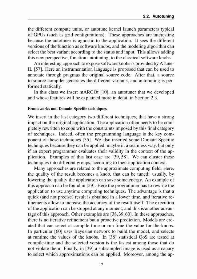
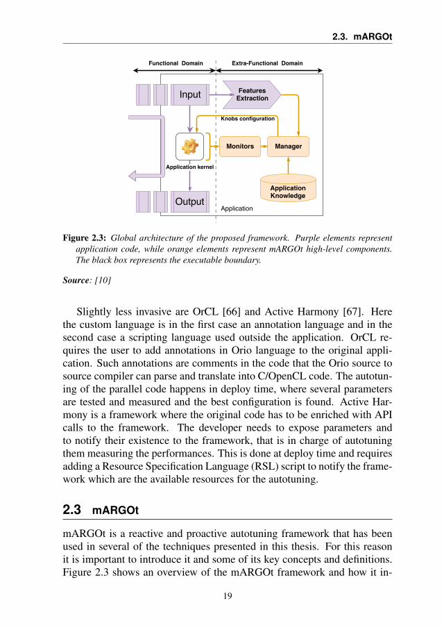
Figure 2.3: Global architecture of the proposed framework. Purple elements representapplication code, while orange elements represent mARGOt high-level components.The black box represents the executable boundary.
Source: [10]
Slightly less invasive are OrCL [66] and Active Harmony [67]. Herethe custom language is in the first case an annotation language and in thesecond case a scripting language used outside the application. OrCL re-quires the user to add annotations in Orio language to the original appli-cation. Such annotations are comments in the code that the Orio source tosource compiler can parse and translate into C/OpenCL code. The autotun-ing of the parallel code happens in deploy time, where several parametersare tested and measured and the best configuration is found. Active Har-mony is a framework where the original code has to be enriched with APIcalls to the framework. The developer needs to expose parameters andto notify their existence to the framework, that is in charge of autotuningthem measuring the performances. This is done at deploy time and requiresadding a Resource Specification Language (RSL) script to notify the frame-work which are the available resources for the autotuning.
2.3 mARGOt
mARGOt is a reactive and proactive autotuning framework that has beenused in several of the techniques presented in this thesis. For this reasonit is important to introduce it and some of its key concepts and definitions.Figure 2.3 shows an overview of the mARGOt framework and how it in-
19
Chapter 2. Previous work
teracts with an application. In this chapter, we will assume that the targetapplication has a single kernel g that elaborates an input i to generate thedesired output o. However, mARGOt has been designed to be capable ofmanaging different kernels (each one defined block) of an application in acompletely independent way. We also assume that the kernel already ex-poses the software-knobs needed to alter its behavior. Let x = [x1, . . . , xn]the vector of software-knobs, then we define a kernel as o = g(x, i).
Given this abstraction of the target application, we define the end-userrequirements. The metrics of interest (the EFPs) are defined as the vectorm = [m1,m2, . . . ,mn]. If the application programmer is able to find someproperties of the input, we will define such properties as the vector f =[f1, f2, . . . , fn]. Given these definitions, the requirements of the applicationcan be formalized as in Equation 2.1:
max(min) r(x;m | f)s.t. C1 : ω1(x;m | f) ∝ k1 with α1 confidence
C2 : ω2(x;m | f) ∝ k2
. . .
Cn : ωn(x;m | f) ∝ kn
(2.1)
where r is the objective function defined as a composition of any variabledefined either in m or in x by using their mean values. C represents the setof constraints. Each Ci is a constraint expressed as the function ωi, definedover the software-knobs or the EFPs and it must satisfy the relationship∝∈ {<,≤, >,≥} with a threshold value ki. If ωi targets a statistical vari-able it also has to have a confidence αi. Since mARGOt is agnostic to thedistribution of the parameter, the confidence is expressed as an integer co-efficient of its standard deviation (i.e. two times the standard deviation).If there are input features, then the value of the rank function r and theconstraint functions ωi may also depend from f .
The main goal of mARGOt is to solve the following optimization prob-lem: finding the configuration x that satisfies all the constraints C and max-imizes (minimizes) the objective function r, given the current input i. Theapplication must have a configuration. If it is not possible to satisfy allthe constraints, mARGOt will relax some of them, until it finds a feasiblesolution. For this reason, the constraints have a priority. mARGOt startsrelaxing the lowest priority constraints first. Therefore, the end-user is re-quired to give a priority to all the constraints. As shown in Figure 2.3, themARGOt framework is composed of the application manager, the moni-tors, and the application knowledge. In the next subsections, we will seeeach component in detail, and we will conclude this section with someconsiderations on the integration effort required to insert mARGOt in the
20
2.3. mARGOt
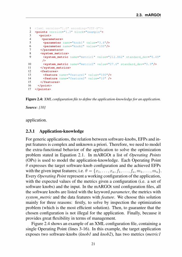
1 <?xml version="1.0" encoding="UTF-8"?>2 <points version="1.3" block="example">3 <point>4 <parameters>5 <parameter name="knob1" value="3.4"/>6 <parameter name="knob2" value="100"/>7 </parameters>8 <system_metrics>9 <system_metric name="metric1" value="212.862" standard_dev="6.49"
/>10 <system_metric name="metric2" value="27.6" standard_dev="0.9"/>11 </system_metrics>12 <features>13 <feature name="feature1" value="100"/>14 <feature name="feature2" value="10" />15 </features>16 </point>17 </points>
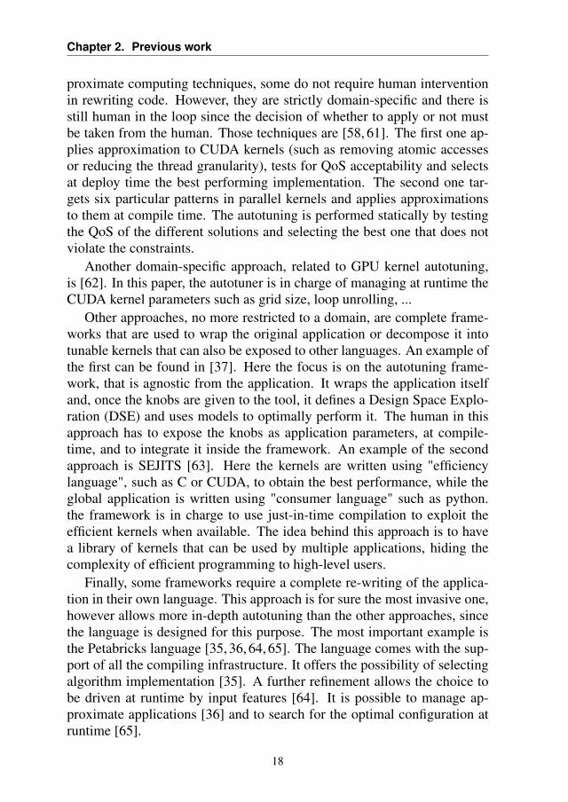
Figure 2.4: XML configuration file to define the application-knowledge for an application.
Source: [10]
application.
2.3.1 Application-knowledge
For generic applications, the relation between software-knobs, EFPs and in-put features is complex and unknown a priori. Therefore, we need to modelthe extra-functional behavior of the application to solve the optimizationproblem stated in Equation 2.1. In mARGOt a list of Operating Points(OPs) is used to model the application-knowledge. Each Operating Pointθ expresses the target software-knob configuration and the achieved EFPswith the given input features; i.e. θ = {x1, . . . , xn, f1, . . . , fn,m1, . . . ,mn}.Every Operating Point represent a working configuration of the application,with the expected values of the metrics given a configuration (i.e. a set ofsoftware knobs) and the input. In the mARGOt xml configuration files, allthe software knobs are listed with the keyword parameter, the metrics withsystem_metric and the data features with feature. We choose this solutionmainly for three reasons: firstly, to solve by inspection the optimizationproblem (which is the most efficient solution). Then, to guarantee that thechosen configuration is not illegal for the application. Finally, because itprovides great flexibility in terms of management.
Figure 2.4 shows an example of an XML configuration file, containing asingle Operating Point (lines 3-16). In this example, the target applicationexposes two software-knobs (knob1 and knob2), has two metrics (metric1
21
Chapter 2. Previous work
and metric2) and it is possible to extract two features from the input (fea-ture1 and feature2). For this reason, the OP is composed of three sections:the software-knobs configuration (lines 4-7), the metric section with the ex-pected performance distribution (lines 8-11), and the related feature cluster(lines 12-15).
The OP list is a required input and mARGOt is agnostic to the methodol-ogy used to obtain it. Typically this is a design-time task, known as DesignSpace Exploration (DSE) in literature. It is a well-known problem, aimedat finding the Pareto Set. There are several previous approaches to findit efficiently [68–70]. The chosen methodology is out of scope from themARGOt perspective.
Moreover, mARGOt has the capability of changing the application knowl-edge at runtime.
2.3.2 Monitors
It is important to observe the behavior of the application and the platformduring the execution. For this reason, mARGOt has monitors. They areof critical importance because they provide feedback information. As wehave seen, application knowledge defines the expected behavior which maychange because of factors that are external from the application. For exam-ple, a power capper reduces the frequency of the processor. We expect theapplication to notice the performance degradation, and to react by changingits configuration to compensate. This is only possible thanks to feedbackinformation.
If it is not possible to monitor an EFP at runtime, mARGOt can stillwork. It will operate in an open-loop, basing its decision only on the ex-pected behavior.
2.3.3 Application Manager
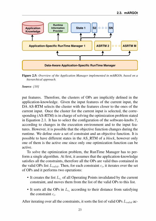
This component is the core of the mARGOt dynamic autotuner since itprovides the self-optimization capability. It is implemented using a hierar-chical structure, as shown in Figure 2.5, where each level of the hierarchytargets a specific problem. The Data-Aware Application-Specific Run-TimeManager (DA AS-RTM) provides a unified interface to application devel-opers to set or change the application requirements, to set or change theapplication-knowledge and to retrieve the most suitable configuration x.Internally, the DA AS_RTM clusters the application-knowledge accord-ing to the input features f by creating an Application-Specific Run-TimeManager (AS-RTM) for each cluster of Operating Points with the same in-
22
2.3. mARGOt
Data-Aware Application-Specific RunTime Manager
Application-Specific RunTime Manager 1 ASRTM 2
Application Knowledge
Runtime Information
Provider State 1 S2 SN
ASRTM M
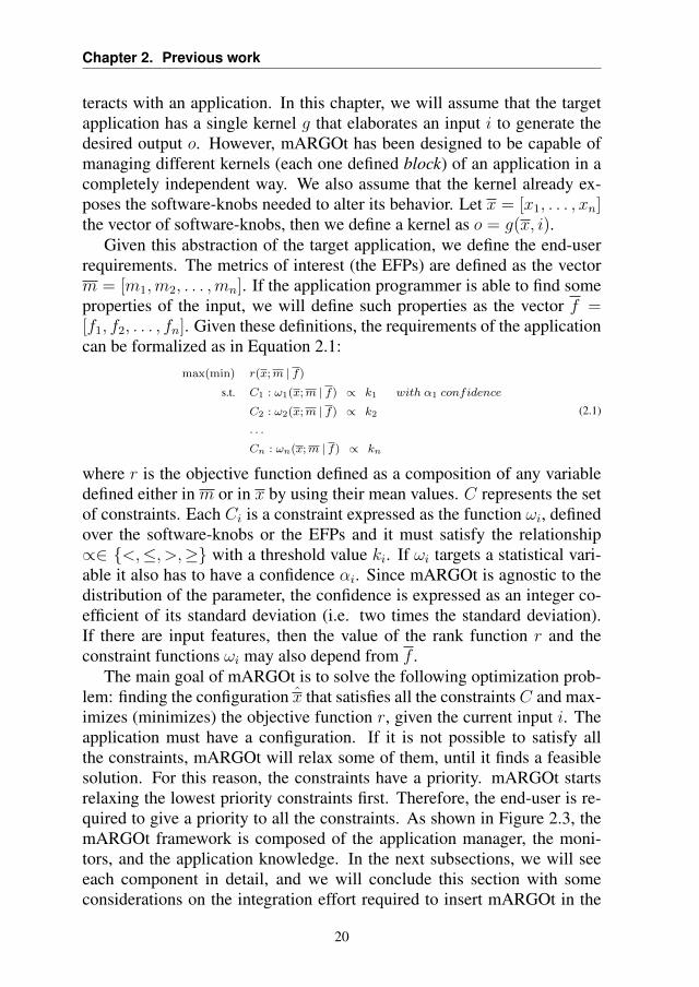
Figure 2.5: Overview of the Application Manager implemented in mARGOt, based on ahierarchical approach.
Source: [10]
put features. Therefore, the clusters of OPs are implicitly defined in theapplication-knowledge. Given the input features of the current input, theDA AS-RTM selects the cluster with the features closer to the ones of thecurrent input. Once the cluster for the current input is selected, the corre-sponding (AS-RTM) is in charge of solving the optimization problem statedin Equation 2.1. It has to select the configuration of the software-knobs x,according to changes in the execution environment and to the input fea-tures. However, it is possible that the objective function changes during theruntime. We define state a set of constraint and an objective function. It ispossible to have different states in the AS_RTM of a block, however onlyone of them is the active one since only one optimization function can beactive.
To solve the optimization problem, the RunTime Manager has to per-form a single algorithm. At first, it assumes that the application-knowledgesatisfies all the constraints, therefore all the OPs are valid thus contained inthe valid OPs list Lvalid. Then, for each constraint ci, it iterates over the setof OPs and it performs two operations:
• It creates the list Lci of all Operating Points invalidated by the currentconstraint, and moves them from the list of the valid OPs to this list.
• It sorts all the OPs in Lci according to their distance from satisfyingthe constraint ci.
After iterating over all the constraints, it sorts the list of valid OPs Lvalid ac-
23
Chapter 2. Previous work
cording to the objective function r. If the list of the valid Operative Pointsis not empty, it returns the one that maximizes the objective function. Oth-erwise, mARGOt iterates over the constraints according to their priority, inreverse order, until it finds a constraint ci with a non-empty Lci . Then thebest OP is the closest to satisfy the constraint ci, i.e. Lci [0]. This algorithmmust always return a single OP.
2.3.4 Integration Effort
While designing the framework, we focused on three points to ease theintegration effort:
• separation of concerns between functional and extra-functional prop-erties.
• limit the intrusiveness as much as possible.
• ease of use of the instrumentation code.
However, it is still required to the end-user or to the application developerto identify constraints, requirements, software knobs, and input features.
To ease the integration process, we provide a utility tool that generatesa high-level interface for the target application. This tool takes as inputtwo XML files that describe the extra-functional properties of interest. Inparticular, the main configuration file describes the adaptation layer, andthe second configuration file describes the list of known operating points,as seen in Figure 2.4. The main configuration file defines:
1. The monitors of interest for the application;
2. The optimization parameters, i.e. the EFPs of interest, software-knobs,and input features;
3. The optimization problem stated in Equation 2.1.
Starting from these configuration files, the utility tool generates a librarycontaining all the required glue code to hide, as much as possible, the im-plementation details. In particular, this library exposes five functions to thedevelopers:
• init. A global function that initializes the data structures.
• update. A function that updates the software-knobs of a block withthe optimal configuration found.
• start_monitor. A function that starts all the monitors of a block.
24
2.4. Summary
• stop_monitor A function that stops all the monitors of a block.
• log A function that logs the monitors of a block.
This library hides the details of the basic usage of the framework. However,if application developers require more advanced adaptation strategies, forexample changing the application requirements at runtime, they will needto use the real mARGOt interface, since the high-level interface providedby the generated library will no more be enough.
2.4 Summary
In this chapter, we have seen the background and the state of the art in theautotuning field. We explored it through two perspectives, the time of au-totuning and the intrusiveness. In a second moment we have introducedmARGOt, an autotuning framework that we developed, and we will seehow we used it to enhance applications in Chapter 4, Chapter 9 and Chap-ter 6.
25

CHAPTER3Methodology
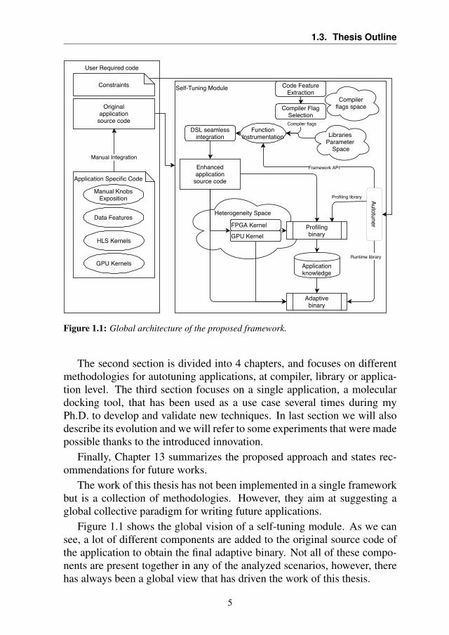
This chapter is focused on explaining the conceptual framework that is be-hind the work done in this thesis. As already mentioned in Chapter 2, thisframework has not been implemented but it is an important reference modelthat has guided me through all my work. For this reason, we could call it ameta-framework, since it is an ideal entity. It is fundamental to understandthe whole work done in this thesis since it has always driven the research.
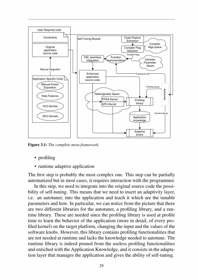
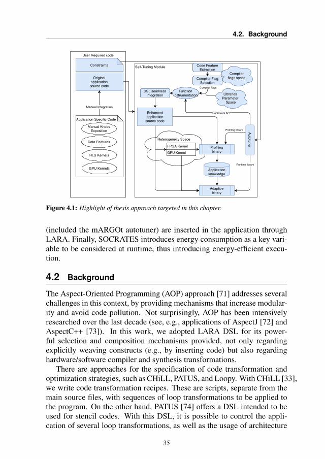
We consider future applications as a sequence of self-tuning modules,that can adapt at runtime to the changing condition of the platform theyare executed on. Moreover, they shall be able to exploit the heterogene-ity, whenever available, and organize themselves to run each section of theapplication on the hardware that is most suitable to the computations thatare being executed (i.e. if the application has a strong control-flow boundsection, should be running on the CPU, while if there is a section with a lotof data-parallel computation it should run on the GPU). However, to reachthis goal the original application needs to be changed and integrated by thedeveloper. As we can see in Figure 3.1, there are two different areas. Thefirst one is the user required code, and the second is the actual self-tuningmodule.
The user required code can be divided into two macro-areas, the first
27
Chapter 3. Methodology
being the mandatory code (i.e. the application code and the constraint con-figuration) and the second the application-specific code, which is useful tohave in a module but not mandatory. Application-specific code consists ofpieces of code that have to be manually or semi-manually integrated into theoriginal application to create more opportunities for the autotuning of theapplication during the runtime. Examples of application-specific code arethe manual exposition of software knobs, such as searching accuracy-timeto solution tradeoffs, or when inserting heterogeneity in a homogeneousapplication. The addition of the application-specific code to the applicationhas to be done at design time since it needs to be performed by a program-mer. More in detail, the operation that we envision in this category are:
• Manual Knob Exposition: the application is analyzed to find and ex-pose some software knobs that were no present in the original applica-tion formulation. These knobs can be related to performance-accuracytradeoffs, or other parameters that were in the original application de-cided once (such as command line parameters) and never changed dur-ing the run of the application itself. An example of this analysis isdone in Chapter 9.
• Data Features: an analysis of the input data is performed, to take ad-vantage during the runtime of some features of the input. This usuallymeans that we want to cluster the set of inputs and manage the clustersin different ways during the runtime since we can take advantage ofthe features of the punctual input that we found with this analysis. Anexample of this is done in Chapter 6
• Heterogeneous Kernels: the application is analyzed and a hotspot ker-nel is ported to a more suitable architecture, that can be the GPU oran FPGA. The kernel is integrated into the original application flow,following the traditional approach of heterogeneous computing. Anexample of this can be found in Chapter 10.
The important section of Figure 3.1 is the right part, what is called theself-tuning module. This module is the key component of future applica-tions. The original application is enriched with several components, thusbecoming able to perform self-management during its runtime. We can no-tice from the picture that there are three main phases to obtain the ultimategoal of having an adaptive binary (which is the self-tuning module runtimeimplementation):
• create the enhanced application source code
28
User Required code
Self-Tuning Module
Heterogeneity Space
Originalapplication
source code
Code FeatureExtraction
Compilerflags space
Compiler flags
Compiler FlagSelection
Libraries Parameter
Space
DSL seamlessintegration
Enhancedapplication
source code
Profilingbinary
Applicationknowledge
Adaptivebinary
Runtime library
Framework API
Autotuner
Profiling library
Manual Integration
Application Specific Code
Data Features
HLS Kernels
GPU Kernels
FPGA Kernel
GPU Kernel
Constraints
Manual KnobsExposition
FunctionInstrumentation
Figure 3.1: The complete meta-framework.
• profiling
• runtime adaptive application
The first step is probably the most complex one. This step can be partiallyautomatized but in most cases, it requires interaction with the programmer.
In this step, we need to integrate into the original source code the possi-bility of self-tuning. This means that we need to insert an adaptivity layer,i.e. an autotuner, into the application and teach it which are the tunableparameters and how. In particular, we can notice from the picture that thereare two different libraries for the autotuner, a profiling library, and a run-time library. These are needed since the profiling library is used at profiletime to learn the behavior of the application (more in detail, of every pro-filed kernel) on the target platform, changing the input and the values of thesoftware knobs. However, this library contains profiling functionalities thatare not needed at runtime and lacks the knowledge needed to autotune. Theruntime library is indeed pruned from the useless profiling functionalitiesand enriched with the Application Knowledge, and it consists in the adapta-tion layer that manages the application and gives the ability of self-tuning.
29
Chapter 3. Methodology
In this thesis, we used the mARGOt autotuner, described in detail inSection 2.3.
However, the autotuner alone is unable to do anything. To enable theself-tuning, we also need to provide the autotuner the software knobs. Thiswork can be done manually, as we already mentioned, or in a semi-automaticalway. Indeed, the top right part of the self-tuning module picture focuseson this use case. Some features are common to all the applications, suchas compiler flags. Other possible knobs derive from libraries, that may beused in the program. In both these cases, it is possible to semi-automaticallyinsert these knobs in the application code. We need to instrument the ap-plication at function level. In this way, we can learn the behavior of thedifferent sets of parameters and compiler flags on these functions. We willsee in Chapter 4 a study in this direction. The autotuner API can also beinserted during the function instrumentation, and they are needed to profilethe behavior of the function. The last way to enrich an application is, aswe already have seen, to insert some heterogeneous kernels. Sadly thereis no way to do this automatically since as we will see in Chapter 10 evendirective-based approaches require heavy modification of the original ap-plication source code.
Once all of these operations are done, and we have obtained the enrichedcode, a training phase occurs to extract knowledge from the application. Adesign space exploration has to be performed, to find the Pareto optimalfrontier in the available parameter space. Previous research [68–70] haveproposed methodologies to obtain the Pareto set. In this thesis, however, themethodology used to search the Pareto set is not important, and will not beinvestigated. This operation allows building the Application Knowledge,where the interaction of the software knobs with the evaluation metrics onthe target machine is stored.
Once the Application Knowledge is obtained, it is possible to build theadaptive binary. This binary is the objective of the work of this thesis, andconsists in the revised version of the original application as a sequence ofself-tuning modules, able to adapt to the changing condition of the platformwhere they have been trained, or to changes in the requirements and theinput data.
30

Part I
General Autotuning Techniques
31

CHAPTER4A Seamless Online Compiler and System
Runtime Autotuning Framework
In this chapter, we address the problem of fine-grain autotuning, enablingthe change of compiler flags across different functions or the number ofinvolved OpenMP threads, with the final purpose of having the target ap-plication always working in the most efficient configuration. In particular,we propose SOCRATES, an approach where several tools are joined to-gether to reach the self-tuning capability of the application. Moreover, wefocus on reaching this goal with as little intrusiveness as possible, to easethe adoption of this solution by the programmers and to avoid introducingsubstantial changes in the original codebase. We demonstrate that thanksto SOCRATES we are able to maintain the running application in its op-timal configuration (in terms of efficiency) while the objective function orthe underlying platform change.
4.1 Introduction
Thanks to the continuous evolution of computing platforms, achieving per-formance portability of applications is a difficult task for developers. Per-
33
Chapter 4. A Seamless Online Compiler and System Runtime AutotuningFramework
formances are strongly dependent on the underlying platform and somecharacteristics of the input data. Moreover, they are also influenced bythe system runtime. The autotuning approach has been proposed as thesolution to this problem. Indeed, having code able to adapt to differentplatforms and conditions could enable performance portability. However,this approach has several unresolved questions. Among them, we can men-tion that writing such code needs a flexible and high-level language capableto express functional aspects, without constraining the implementation. Inthis way, it could be customized later, when the platform is decided, thusgenerating a program optimized for that platform.
As we have seen in Chapter 2, several approaches have been proposed,from the less intrusive but more restricted ones to rewriting completely theapplication to obtain adaptation. The target of these approaches is to givethe autotuning capabilities to the application, thus finding the best config-uration for the target platform. Usually, the less intrusive solution aims atfinding one best-fit-all solution, without considering that the environmentcan change. Indeed, the workload may change, or the resource managermay allocate new cores to the application during the runtime. The solu-tions able to target these opportunities are the dynamic autotuners. How-ever, their drawback is that they require a high level of intrusiveness in theoriginal application.
In this chapter, we aim at obtaining a dynamic solution able to adaptat runtime changes of the configuration with an approach that has as littleintrusiveness as possible. Indeed, configuring some extra-functional prop-erties such as compiler flags and/or number of OpenMP threads can be nottrivial if we want to always have the optimal configuration whenever the ex-ternal conditions of the application are changing. This chapter introducesthe SOCRATES approach. With this approach, we aim at offering the run-time autotuning of these Extra-Functional parameters at function level, witha framework that does not require any modification to the original applica-tion.
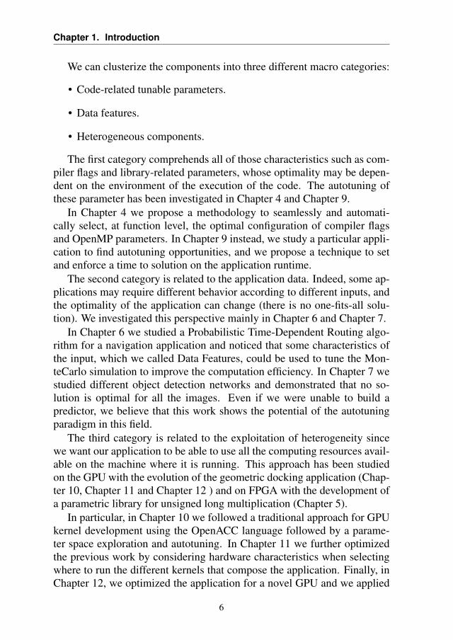
Figure 4.1 shows the components of the global autotuning vision tar-geted in this chapter. As we can see, most of the components are on theright side, the automatic one, while on the left side there are only the con-straints and the original application source code. The main contributionindeed is the separation of concern: when writing the application, the de-veloper does not need to be concerned with autotuning. After that, in aseparate step, the autotuning is inserted into the application. We use anaspect-oriented language, LARA [12], to achieve the separation of con-cerns. Indeed, in this work, the extra-functional parts of the application
34
4.2. Background
User Required code
Self-Tuning Module
Heterogeneity Space
Originalapplication
source code
Code FeatureExtraction
Compilerflags space
Compiler flags
Compiler FlagSelection
Libraries Parameter
Space
DSL seamlessintegration
Enhancedapplication
source code
Profilingbinary
Applicationknowledge
Adaptivebinary
Runtime library
Framework API
Autotuner
Profiling library
Manual Integration
Application Specific Code
Data Features
HLS Kernels
GPU Kernels
FPGA Kernel
GPU Kernel
Constraints
Manual KnobsExposition
FunctionInstrumentation
Constraints Code FeatureExtraction
Compiler FlagSelection
FunctionInstrumentation Libraries
Parameter Space
Compilerflags space
DSL seamlessintegration
Autotuner
Figure 4.1: Highlight of thesis approach targeted in this chapter.
(included the mARGOt autotuner) are inserted in the application throughLARA. Finally, SOCRATES introduces energy consumption as a key vari-able to be considered at runtime, thus introducing energy-efficient execu-tion.
4.2 Background
The Aspect-Oriented Programming (AOP) approach [71] addresses severalchallenges in this context, by providing mechanisms that increase modular-ity and avoid code pollution. Not surprisingly, AOP has been intensivelyresearched over the last decade (see, e.g., applications of AspectJ [72] andAspectC++ [73]). In this work, we adopted LARA DSL for its power-ful selection and composition mechanisms provided, not only regardingexplicitly weaving constructs (e.g., by inserting code) but also regardinghardware/software compiler and synthesis transformations.
There are approaches for the specification of code transformation andoptimization strategies, such as CHiLL, PATUS, and Loopy. With CHiLL [33],we write code transformation recipes. These are scripts, separate from themain source files, with sequences of loop transformations to be applied tothe program. On the other hand, PATUS [74] offers a DSL intended to beused for stencil codes. With this DSL, it is possible to control the appli-cation of several loop transformations, as well as the usage of architecture
35
Chapter 4. A Seamless Online Compiler and System Runtime AutotuningFramework
extensions (i.e., SSE). Loopy [75] allows the programmer to specify a seriesof loop transformations which are then automatically applied and guaran-teed to be correct by formal verification. These are specified in a script (asin CHiLL) and are applied to the internal polyhedral representation.
Tuning the OpenMP parameters is not a novelty, since it has alreadybeen proposed in [76–78]. There the focus is on automatic parallelizationof code with automatic selection of parameters done in a second phase. Theapproach of these works focuses on finding the one-fit-all solution for thegiven platform, without considering dynamic autotuning.
Overall, the proposed approach improves the state of the art thanks to theflexibility of its components: it allows to decouple the autotuning problemfrom writing the application and inserts dynamical autotuning that considerthe evolution of the system in taking the optimal decision.
4.3 Proposed Methodology
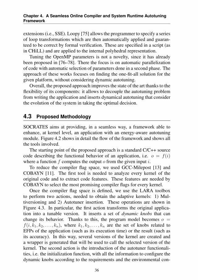
SOCRATES aims at providing, in a seamless way, a framework able toenhance, at kernel level, an application with an energy-aware autotuningmodule. Figure 4.2 shows in detail the flow of the framework and shows allthe tools involved.
The starting point of the proposed approach is a standard C/C++ sourcecode describing the functional behavior of an application, i.e. o = f(i)where a function f computes the output o from the given input i.
To reduce the compiler flag space, we used GCC-Milepost [13] andCOBAYN [11]. The first tool is needed to analyze every kernel of theoriginal code and to extract code features. These features are needed byCOBAYN to select the most promising compiler flags for every kernel.
Once the compiler flag space is defined, we use the LARA toolboxto perform two actions, needed to obtain the adaptive kernels: 1) Mul-tiversioning and 2) Autotuner insertion. These operations are shown inFigure 4.3. In particular, the first action transforms the original applica-tion into a tunable version. It inserts a set of dynamic knobs that canchange its behavior. Thanks to this, the program model becomes o =f(i, k1, k2, . . . , kn), where k1, k2, . . . , kn are the set of knobs related toEFPs of the application (such as its execution time) or the result (such asits accuracy). In this way, several versions of the kernel are created anda wrapper is generated that will be used to call the selected version of thekernel. The second action is the introduction of the autotuner functionali-ties, i.e. the initialization function, with all the information to configure thedynamic knobs according to the requirements and the environmental con-
36
4.3. Proposed Methodology
Figure 4.2: Tool flow of the SOCRATES approach from the original application sourcecode to the generation of the application adaptive binary.
Source: [79]
dition. Moreover, it inserts the autotuner functions that wrap the kernel calland monitor its behavior. In particular, three of these functions are required:start, update and stop. The first function will start the monitoring system,the second will select the version of the kernel according to the monitorvalues and the third will stop the monitoring system. In the example, weonly show an application with a single kernel, but the strong point of thismethodology is that it can be applied on more than one kernel.
After the LARA step, we have obtained the Enhanced application code,which needs to be profiled in order to create the application knowledgerequired by the final adaptive application binary. This is done by run-ning a profiling campaign on all the available alternative kernels, collectingtheir behavior on the underlying architecture. Finally, using the application
37
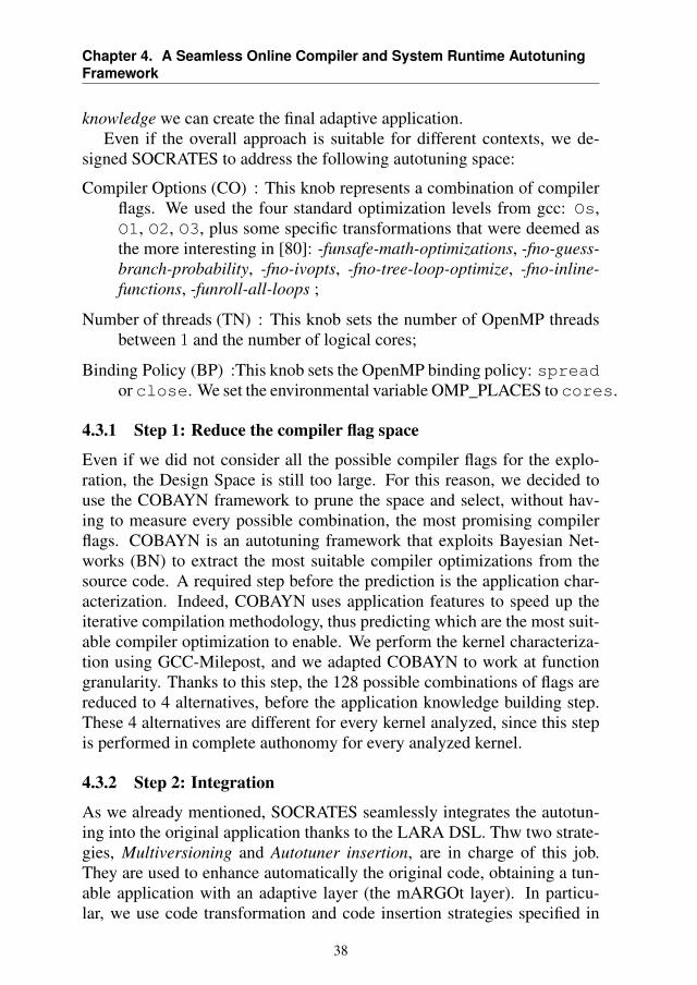
Chapter 4. A Seamless Online Compiler and System Runtime AutotuningFramework
knowledge we can create the final adaptive application.Even if the overall approach is suitable for different contexts, we de-
signed SOCRATES to address the following autotuning space:
Compiler Options (CO) : This knob represents a combination of compilerflags. We used the four standard optimization levels from gcc: Os,O1, O2, O3, plus some specific transformations that were deemed asthe more interesting in [80]: -funsafe-math-optimizations, -fno-guess-branch-probability, -fno-ivopts, -fno-tree-loop-optimize, -fno-inline-functions, -funroll-all-loops ;
Number of threads (TN) : This knob sets the number of OpenMP threadsbetween 1 and the number of logical cores;
Binding Policy (BP) :This knob sets the OpenMP binding policy: spreador close. We set the environmental variable OMP_PLACES to cores.
4.3.1 Step 1: Reduce the compiler flag space
Even if we did not consider all the possible compiler flags for the explo-ration, the Design Space is still too large. For this reason, we decided touse the COBAYN framework to prune the space and select, without hav-ing to measure every possible combination, the most promising compilerflags. COBAYN is an autotuning framework that exploits Bayesian Net-works (BN) to extract the most suitable compiler optimizations from thesource code. A required step before the prediction is the application char-acterization. Indeed, COBAYN uses application features to speed up theiterative compilation methodology, thus predicting which are the most suit-able compiler optimization to enable. We perform the kernel characteriza-tion using GCC-Milepost, and we adapted COBAYN to work at functiongranularity. Thanks to this step, the 128 possible combinations of flags arereduced to 4 alternatives, before the application knowledge building step.These 4 alternatives are different for every kernel analyzed, since this stepis performed in complete authonomy for every analyzed kernel.
4.3.2 Step 2: Integration
As we already mentioned, SOCRATES seamlessly integrates the autotun-ing into the original application thanks to the LARA DSL. Thw two strate-gies, Multiversioning and Autotuner insertion, are in charge of this job.They are used to enhance automatically the original code, obtaining a tun-able application with an adaptive layer (the mARGOt layer). In particu-lar, we use code transformation and code insertion strategies specified in
38
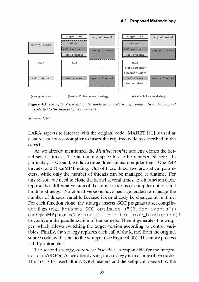
4.3. Proposed Methodology
Figure 4.3: Example of the automatic application code transformation from the originalcode (a) to the final adaptive code (c).
Source: [79]
LARA aspects to interact with the original code. MANET [81] is used asa source-to-source compiler to insert the required code as described in theaspects.
As we already mentioned, the Multiversioning strategy clones the ker-nel several times. The autotuning space has to be represented here. Inparticular, as we said, we have three dimensions: compiler flags, OpenMPthreads, and OpenMP binding. Out of these three, two are statical param-eters, while only the number of threads can be managed at runtime. Forthis reason, we need to clone the kernel several times. Each function clonerepresents a different version of the kernel in terms of compiler options andbinding strategy. No cloned versions have been generated to manage thenumber of threads variable because it can already be changed at runtime.For each function clone, the strategy inserts GCC pragmas to set compila-tion flags (e.g., #pragma GCC optimize ("O3,fno-ivopts"))and OpenMP pragmas (e.g., #pragma omp for proc_bind(close))to configure the parallelization of the kernels. Then it generates the wrap-per, which allows switching the target version according to control vari-ables. Finally, the strategy replaces each call of the kernel from the originalsource code, with a call to the wrapper (see Figure 4.3b). The entire processis fully automated.
The second strategy, Autotuner insertion, is responsible for the integra-tion of mARGOt. As we already said, this strategy is in charge of two tasks.The first is to insert all mARGOt headers and the setup call needed by the
39
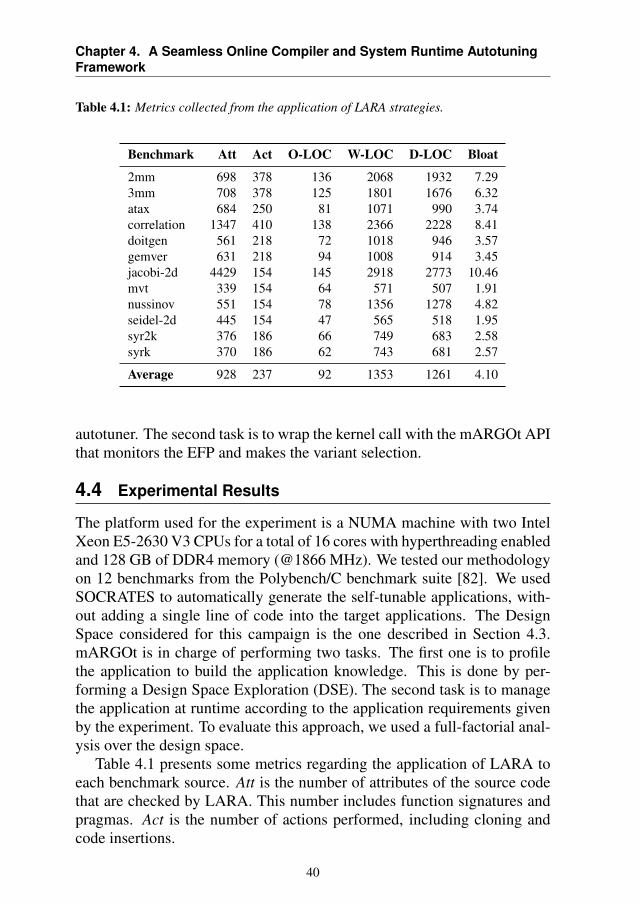
Chapter 4. A Seamless Online Compiler and System Runtime AutotuningFramework
Table 4.1: Metrics collected from the application of LARA strategies.
Benchmark Att Act O-LOC W-LOC D-LOC Bloat
2mm 698 378 136 2068 1932 7.293mm 708 378 125 1801 1676 6.32atax 684 250 81 1071 990 3.74correlation 1347 410 138 2366 2228 8.41doitgen 561 218 72 1018 946 3.57gemver 631 218 94 1008 914 3.45jacobi-2d 4429 154 145 2918 2773 10.46mvt 339 154 64 571 507 1.91nussinov 551 154 78 1356 1278 4.82seidel-2d 445 154 47 565 518 1.95syr2k 376 186 66 749 683 2.58syrk 370 186 62 743 681 2.57
Average 928 237 92 1353 1261 4.10
autotuner. The second task is to wrap the kernel call with the mARGOt APIthat monitors the EFP and makes the variant selection.
4.4 Experimental Results
The platform used for the experiment is a NUMA machine with two IntelXeon E5-2630 V3 CPUs for a total of 16 cores with hyperthreading enabledand 128 GB of DDR4 memory (@1866 MHz). We tested our methodologyon 12 benchmarks from the Polybench/C benchmark suite [82]. We usedSOCRATES to automatically generate the self-tunable applications, with-out adding a single line of code into the target applications. The DesignSpace considered for this campaign is the one described in Section 4.3.mARGOt is in charge of performing two tasks. The first one is to profilethe application to build the application knowledge. This is done by per-forming a Design Space Exploration (DSE). The second task is to managethe application at runtime according to the application requirements givenby the experiment. To evaluate this approach, we used a full-factorial anal-ysis over the design space.
Table 4.1 presents some metrics regarding the application of LARA toeach benchmark source. Att is the number of attributes of the source codethat are checked by LARA. This number includes function signatures andpragmas. Act is the number of actions performed, including cloning andcode insertions.
40
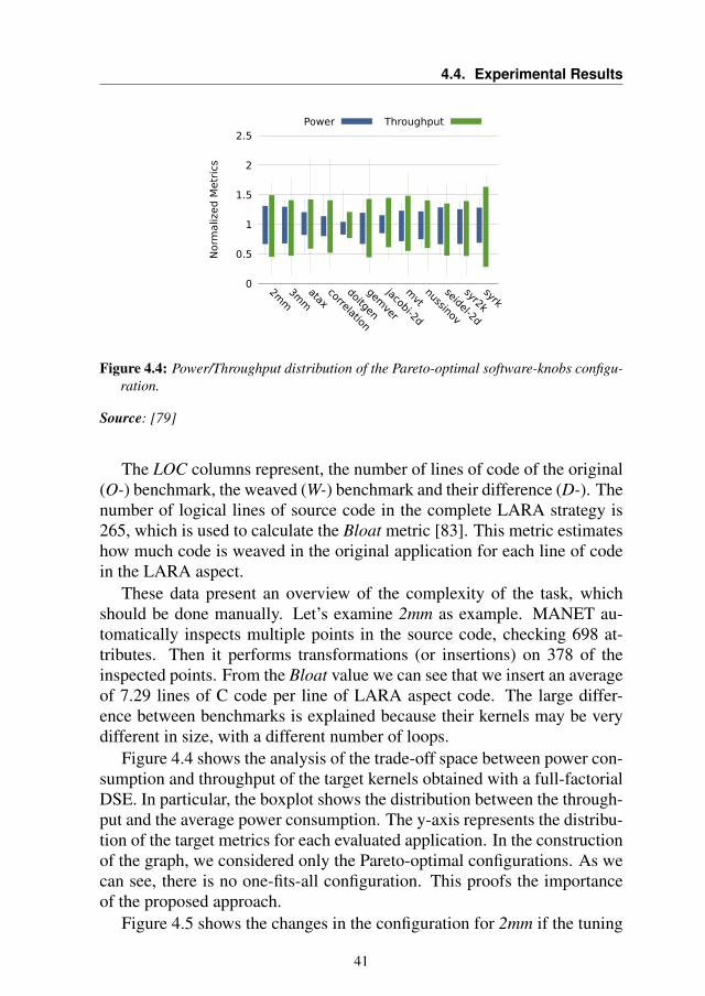
4.4. Experimental Results
0
0.5
1
1.5
2
2.5
2mm
3mm
ataxcorrelation
doitgen
gemver
jacobi-2d
mvt
nussinov
seidel-2d
syr2k
syrk
Norm
aliz
ed
Metr
ics
Power Throughput
Figure 4.4: Power/Throughput distribution of the Pareto-optimal software-knobs configu-ration.
Source: [79]
The LOC columns represent, the number of lines of code of the original(O-) benchmark, the weaved (W-) benchmark and their difference (D-). Thenumber of logical lines of source code in the complete LARA strategy is265, which is used to calculate the Bloat metric [83]. This metric estimateshow much code is weaved in the original application for each line of codein the LARA aspect.
These data present an overview of the complexity of the task, whichshould be done manually. Let’s examine 2mm as example. MANET au-tomatically inspects multiple points in the source code, checking 698 at-tributes. Then it performs transformations (or insertions) on 378 of theinspected points. From the Bloat value we can see that we insert an averageof 7.29 lines of C code per line of LARA aspect code. The large differ-ence between benchmarks is explained because their kernels may be verydifferent in size, with a different number of loops.
Figure 4.4 shows the analysis of the trade-off space between power con-sumption and throughput of the target kernels obtained with a full-factorialDSE. In particular, the boxplot shows the distribution between the through-put and the average power consumption. The y-axis represents the distribu-tion of the target metrics for each evaluated application. In the constructionof the graph, we considered only the Pareto-optimal configurations. As wecan see, there is no one-fits-all configuration. This proofs the importanceof the proposed approach.
Figure 4.5 shows the changes in the configuration for 2mm if the tuning
41
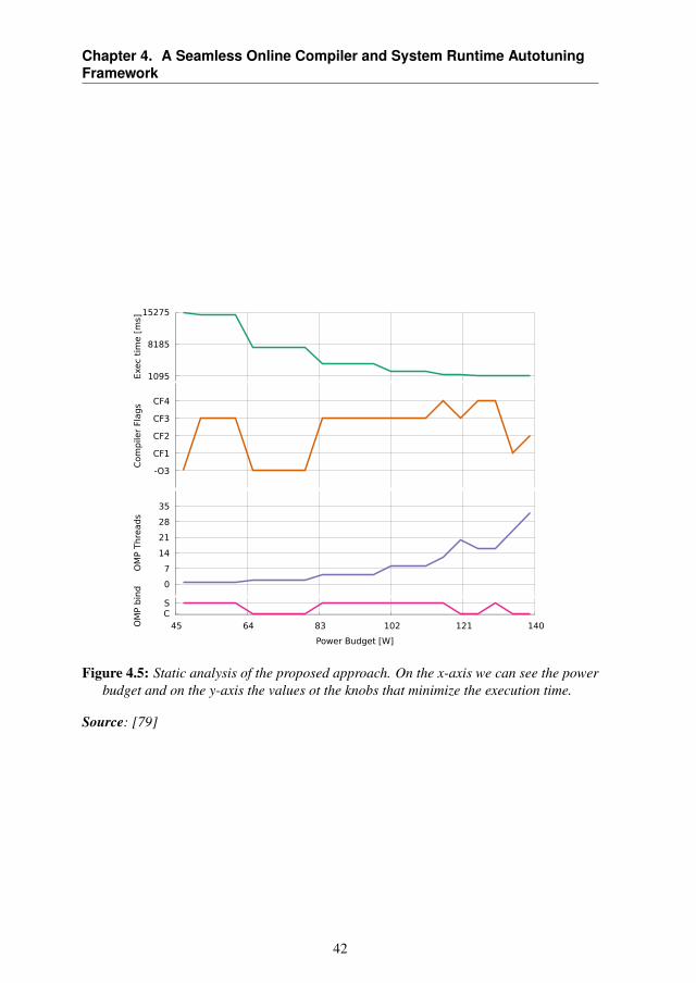
Chapter 4. A Seamless Online Compiler and System Runtime AutotuningFramework
1095
8185
15275
Exe
c ti
me [
ms]
-O3
CF1
CF2
CF3
CF4
Com
pile
r Fl
ags
0
7
14
21
28
35
OM
P T
hre
ads
CS
45 64 83 102 121 140OM
P b
ind
Power Budget [W]
Figure 4.5: Static analysis of the proposed approach. On the x-axis we can see the powerbudget and on the y-axis the values ot the knobs that minimize the execution time.
Source: [79]
42
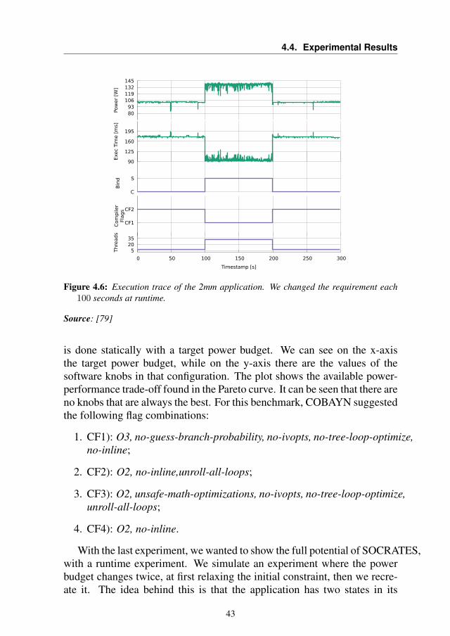
4.4. Experimental Results
80 93
106 119 132 145
Pow
er
[W]
90
125
160
195
Exe
c Ti
me [
ms]
C
S
Bin
d
CF1
CF2
Com
pile
rFl
ags
5 20 35
0 50 100 150 200 250 300
Thre
ads
Timestamp [s]
Figure 4.6: Execution trace of the 2mm application. We changed the requirement each100 seconds at runtime.
Source: [79]
is done statically with a target power budget. We can see on the x-axisthe target power budget, while on the y-axis there are the values of thesoftware knobs in that configuration. The plot shows the available power-performance trade-off found in the Pareto curve. It can be seen that there areno knobs that are always the best. For this benchmark, COBAYN suggestedthe following flag combinations:
1. CF1): O3, no-guess-branch-probability, no-ivopts, no-tree-loop-optimize,no-inline;
2. CF2): O2, no-inline,unroll-all-loops;
3. CF3): O2, unsafe-math-optimizations, no-ivopts, no-tree-loop-optimize,unroll-all-loops;
4. CF4): O2, no-inline.
With the last experiment, we wanted to show the full potential of SOCRATES,with a runtime experiment. We simulate an experiment where the powerbudget changes twice, at first relaxing the initial constraint, then we recre-ate it. The idea behind this is that the application has two states in its
43
Chapter 4. A Seamless Online Compiler and System Runtime AutotuningFramework
execution, the energy save configuration and the throughput configuration.The first one optimizes the Throughput per Watt2 (Thr/W 2), while the sec-ond is interested only in the throughput. Figure 4.6 reports the executiontrace of the target application (2mm). We can notice that the parameter setchanges whenever (at 100 and 200 seconds) we change the target configu-ration. mARGOt adapts the knobs to meet the configuration requirement.
4.5 Summary
This chapter contributes to the thesis by presenting SOCRATES, an auto-tuning framework designed to enable performance portability without re-quiring user contribution. We have shown by applying SOCRATES to theOpenMP polybench suite that it enables application adaptivity at runtime.It allows to always select the better configuration according to runtime con-straints that can change during the application lifetime.
The outcome of this work has been published in the Design, Automationand Test in Europe Conference, 2018 [79].
44
CHAPTER5A library for tunable Multipliers Hardware
Accelerators
In this chapter, we will consider the first heterogenous autotuning tech-nique, targeting Field Programmable Gate Arrays (FPGA). In this context,we will create a tunable library that follows the idea of others in literaturethat can generate different accelerators for an important primitive operationin computer science, the large unsigned multiplication. This operation rep-resents a significant computation effort in some cryptographic techniques.Thus, the use of dedicated hardware is an appealing solution to improveperformance or efficiency.
The library can generate several large integer multipliers with differentcharacteristics in terms of throughput and area occupancy through HighLevel Synthesis. In this way, even programmers that are not expert in usingor programming FPGA can easily and quickly create accelerators for theirapplication. The goal of this chapter is to provide a library that enables theend-user to explore a wide range of possibilities, in terms of performanceand resource utilization, without requiring them to know implementationand synthesis details. Experimental results show the large flexibility of thegenerated architectures and that the generated Pareto-set of multipliers can
45
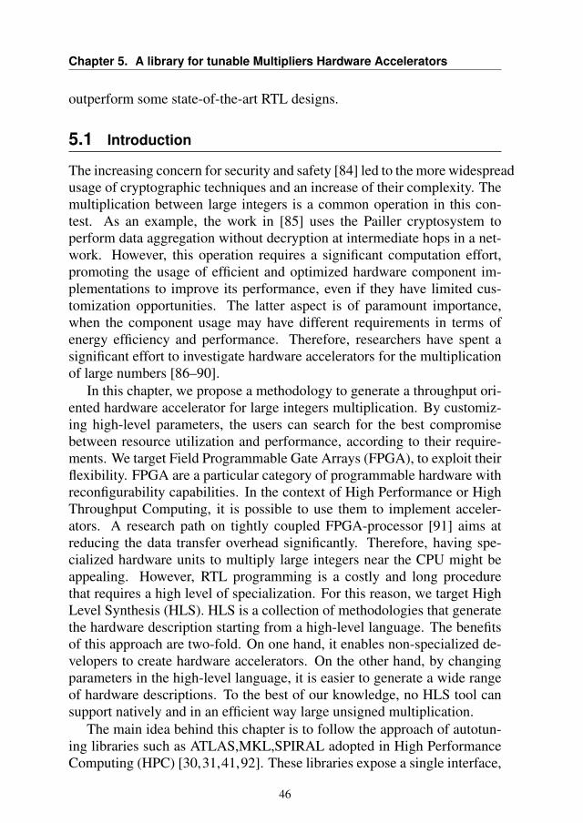
Chapter 5. A library for tunable Multipliers Hardware Accelerators
outperform some state-of-the-art RTL designs.
5.1 Introduction
The increasing concern for security and safety [84] led to the more widespreadusage of cryptographic techniques and an increase of their complexity. Themultiplication between large integers is a common operation in this con-test. As an example, the work in [85] uses the Pailler cryptosystem toperform data aggregation without decryption at intermediate hops in a net-work. However, this operation requires a significant computation effort,promoting the usage of efficient and optimized hardware component im-plementations to improve its performance, even if they have limited cus-tomization opportunities. The latter aspect is of paramount importance,when the component usage may have different requirements in terms ofenergy efficiency and performance. Therefore, researchers have spent asignificant effort to investigate hardware accelerators for the multiplicationof large numbers [86–90].
In this chapter, we propose a methodology to generate a throughput ori-ented hardware accelerator for large integers multiplication. By customiz-ing high-level parameters, the users can search for the best compromisebetween resource utilization and performance, according to their require-ments. We target Field Programmable Gate Arrays (FPGA), to exploit theirflexibility. FPGA are a particular category of programmable hardware withreconfigurability capabilities. In the context of High Performance or HighThroughput Computing, it is possible to use them to implement acceler-ators. A research path on tightly coupled FPGA-processor [91] aims atreducing the data transfer overhead significantly. Therefore, having spe-cialized hardware units to multiply large integers near the CPU might beappealing. However, RTL programming is a costly and long procedurethat requires a high level of specialization. For this reason, we target HighLevel Synthesis (HLS). HLS is a collection of methodologies that generatethe hardware description starting from a high-level language. The benefitsof this approach are two-fold. On one hand, it enables non-specialized de-velopers to create hardware accelerators. On the other hand, by changingparameters in the high-level language, it is easier to generate a wide rangeof hardware descriptions. To the best of our knowledge, no HLS tool cansupport natively and in an efficient way large unsigned multiplication.
The main idea behind this chapter is to follow the approach of autotun-ing libraries such as ATLAS,MKL,SPIRAL adopted in High PerformanceComputing (HPC) [30,31,41,92]. These libraries expose a single interface,
46
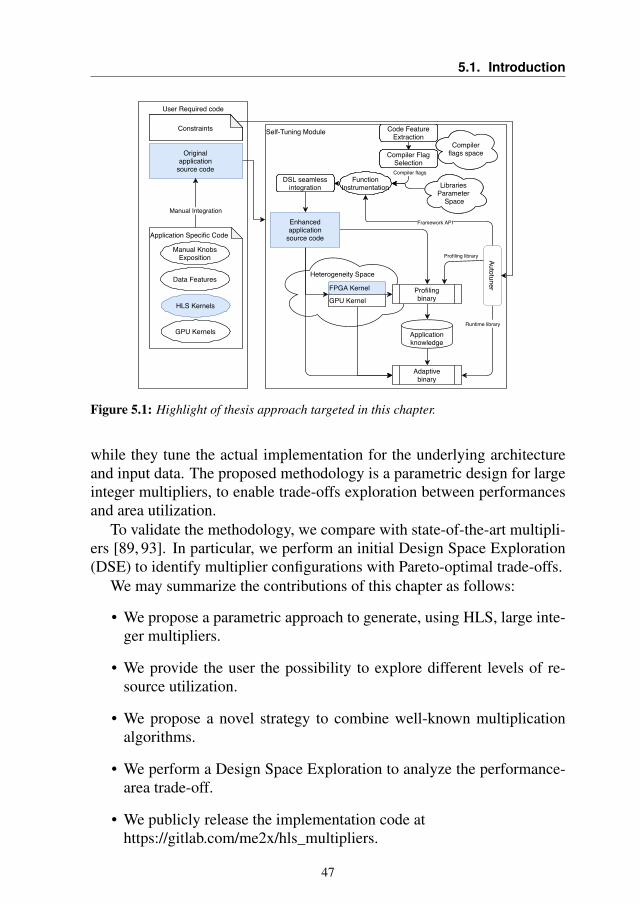
5.1. Introduction
User Required code
Self-Tuning Module
Heterogeneity Space
Originalapplication
source code
Code FeatureExtraction
Compilerflags space
Compiler flags
Compiler FlagSelection
Libraries Parameter
Space
DSL seamlessintegration
Enhancedapplication
source code
Profilingbinary
Applicationknowledge
Adaptivebinary
Runtime library
Framework API
Autotuner
Profiling library
Manual Integration
Application Specific Code
Data Features
HLS Kernels
GPU Kernels
FPGA Kernel
GPU Kernel
Constraints
Manual KnobsExposition
FunctionInstrumentation
Constraints Code FeatureExtraction
Compiler FlagSelection
FunctionInstrumentation Libraries
Parameter Space
Compilerflags space
DSL seamlessintegration
Autotuner
Figure 5.1: Highlight of thesis approach targeted in this chapter.
while they tune the actual implementation for the underlying architectureand input data. The proposed methodology is a parametric design for largeinteger multipliers, to enable trade-offs exploration between performancesand area utilization.
To validate the methodology, we compare with state-of-the-art multipli-ers [89, 93]. In particular, we perform an initial Design Space Exploration(DSE) to identify multiplier configurations with Pareto-optimal trade-offs.
We may summarize the contributions of this chapter as follows:
• We propose a parametric approach to generate, using HLS, large inte-ger multipliers.
• We provide the user the possibility to explore different levels of re-source utilization.
• We propose a novel strategy to combine well-known multiplicationalgorithms.
• We perform a Design Space Exploration to analyze the performance-area trade-off.
• We publicly release the implementation code athttps://gitlab.com/me2x/hls_multipliers.
47
Chapter 5. A library for tunable Multipliers Hardware Accelerators
In the context of the global framework, this chapter focuses on enablingthe heterogeneous computing approach with a different architecture. In thiscase, the focus moves on creating an accelerator on an FPGA. This is onlya first step toward a heterogeneous self-tuning module that relies on thisplatform. It is however important since it creates a starting point for futureapplications, that can exploit the proposed library and can couple it withthe autotuning framework (for example to change the deployed multiplieraccording to constraints on the FPGA area available) and realize a real self-tunable module.
5.2 Background
This section describes the works in the literature related to the proposedapproach. In particular, we focus on two main aspects. At first, we describedifferent implementations of large integer multiplication. Then we analyzeautotuning libraries and how they approach alternative implementations.
Large integer multiplications If we focus on software, the GMP library [94]contains a collection of optimized algorithms. The optimal one is chosenat runtime according to the underlying architecture and operands size. Thislibrary is empirically considered the reference implementation for softwaremultiplication. For example, both the FLINT library [95] and the NTLlibrary [96] exploit GMP in their internal implementation. While soft-ware multiplications focus on the execution time, a hardware implemen-tation must consider multiple extra-functional properties, such as area con-sumption and energy efficiency. Therefore, it is not possible to identifya single optimal solution for a given data size. A large fraction of liter-ature investigates multiplication between small numbers, for example upto 128 bits [90]. An interesting approach has been proposed in a previouswork [93], which employs an Open Source generator to optimize the usageof the Digital Signal Processor (DSP) available on the FPGA. However,it has been optimized for latency and not throughput. Rafferty et al. [89]provide an extensive comparison of different techniques to perform integermultiplications with arbitrary size and inspired us for this work. In par-ticular, it is possible to use four base algorithms: the direct multiplication(Schoolbook), the Comba multiplication, the Karatsuba multiplication, andthe Number Theoretic Transforms (NTT). Direct multiplication exploits thegreatest number of DSPs, limiting its applicability for large numbers. Onthe opposite side, the Comba multiplier uses the least amount of resources,but it is the slowest. In the middle range lies the Karatsuba multiplier. Fi-
48
5.3. Target Class of Multiplication Algorithms
nally, NTT relies on Fourier transform and it requires a significant operandsize (greater than 16384 bits [89]) to outweigh the initialization cost. More-over, it is possible to combine different base algorithms, to leverage theirstrength. We consider the combined approach [89] as the baseline for themultipliers generated by the proposed approach. A significant fraction ofthe related works reported in this section targets FPGA. As previously men-tioned, properly programming these devices with RTL requires experiencedprogrammers. Since our objective is to provide the possibility to performlarge unsigned multiplications to a large audience, we will target HLS. Theproposed library will have to be integrated into the high-level code, andfrom there the HLS tool translates the functional behavior to logic leveland it creates the hardware description [97–100].
Autotuning Libraries The typical workload of HPC includes scientific ap-plications that belong to a wide range of domains. However, these applica-tions typically share several computing-intensive patterns in their hotspots,usually algebraic operations. To implement an efficient code that performssuch tasks requires the knowledge of the underlying architecture, introduc-ing the problem of performance portability. Moreover, the application de-veloper must perform this engineering task for every application. Auto-tuning libraries solve this problem by isolating a small set of performance-critical functionalities with a standard application programming interface(API). The function implementation uses different architecture-specific op-timizations that are automatically applied according to the target platform.In this way, they release the application developer from the optimizationtask. An example of this approach is the BLAS API (Basic Linear AlgebraSubprograms, [29]). The API defines a set of primitives for linear alge-bra, which has become standard for dense linear algebra applications. Forexample, the ATLAS [30] and SPIRAL [31] autotuning libraries exploitthe BLAS interface. We have already analyzed this approach in detail inSubsection 2.2.2.
5.3 Target Class of Multiplication Algorithms
The basic multiplication method, named schoolbook, replicates the paperand pen method that is commonly used. Its drawback is that it requires avery large amount of load and store to update the result when we considerlarge integers. For this reason, literature investigates alternative multiplica-tion methods. Among all of them, this work targets the intermediate sizeof operands, where the non-optimality of the direct approach starts to be a
49
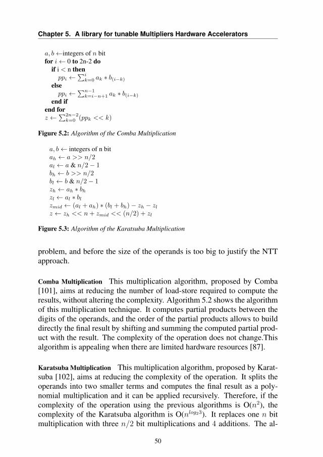
Chapter 5. A library for tunable Multipliers Hardware Accelerators
a, b←integers of n bitfor i← 0 to 2n-2 do
if i < n thenppi ←
∑ik=0 ak ∗ b(i−k)
elseppi ←
∑n−1k=i−n+1 ak ∗ b(i−k)
end ifend forz ←
∑2n−2k=0 (ppk << k)
Figure 5.2: Algorithm of the Comba Multiplication
a, b← integers of n bitah ← a >> n/2al ← a & n/2− 1bh ← b >> n/2bl ← b & n/2− 1zh ← ah ∗ bhzl ← al ∗ blzmid ← (al + ah) ∗ (bl + bh)− zh − zlz ← zh << n+ zmid << (n/2) + zl
Figure 5.3: Algorithm of the Karatsuba Multiplication
problem, and before the size of the operands is too big to justify the NTTapproach.
Comba Multiplication This multiplication algorithm, proposed by Comba[101], aims at reducing the number of load-store required to compute theresults, without altering the complexity. Algorithm 5.2 shows the algorithmof this multiplication technique. It computes partial products between thedigits of the operands, and the order of the partial products allows to builddirectly the final result by shifting and summing the computed partial prod-uct with the result. The complexity of the operation does not change.Thisalgorithm is appealing when there are limited hardware resources [87].
Karatsuba Multiplication This multiplication algorithm, proposed by Karat-suba [102], aims at reducing the complexity of the operation. It splits theoperands into two smaller terms and computes the final result as a poly-nomial multiplication and it can be applied recursively. Therefore, if thecomplexity of the operation using the previous algorithms is O(n2), thecomplexity of the Karatsuba algorithm is O(nlog23). It replaces one n bitmultiplication with three n/2 bit multiplications and 4 additions. The al-
50
5.4. The Proposed Approach
gorithm is reported in Algorithm 5.3 However, recursively applying thealgorithm requires a high number of hardware resources [88].
Karatsuba-Comba Multiplication The Karatsuba algorithm is an appealingapproach to implement a large integer multiplication, due to the lower com-plexity of the operation. Therefore, to mitigate the resource requirements,researchers investigated the possibility to combine the Karatsuba and theComba algorithms [89, 103]. Previous works investigate both software im-plementation [103] and hardware implementation [89]. In particular, thelatter focuses on a hardware implementation that performs a single iterationof the Karatsuba algorithm, while it uses the Comba algorithm to computethe three internal multiplications. Experimental results demonstrate thatthis solution has the lowest latency for operands between 512 and 16384bits [89].
5.4 The Proposed Approach
This section describes the proposed methodology and its implementation.In particular, we propose to use a parametric high-level architecture de-scription and to rely on a High Level Synthesis framework for the actualhardware implementation of the multiplier. At first, we describe the gener-ated architecture template and extract the high-level parameters. Then, wedescribe how these high-level parameters change the generation of the mul-tiplier. Since we are targeting HLS, we aim at exploiting the DSPs availableon the FPGA board. For this reason, we will not decompose the operationto the bit level.
Architecture Template The proposed methodology provides an architecturaltemplate that combines the multiplication algorithms described in Section 5.3,allowing the exploration of a wide range of performance-resources trade-offs. The idea is to use a divide et impera approach. We use recursion toreduce the operands bit-width to increase multiplication efficiency, whilewe use sharing techniques to limit the required amount of logic in the com-putation. Figure 5.4 shows the architecture template and highlights thesizes of the operands across the different layers. We split the multiplicationalgorithm into three phases: (1) Karatsuba Operands Decomposition: werecursively apply the Karatsuba algorithm to reduce the complexity of themultiplication. Every recursion step is named "layer". (2) Products Evalu-ation using the Comba Algorithm. (3) Karatsuba Result Composition: we
51
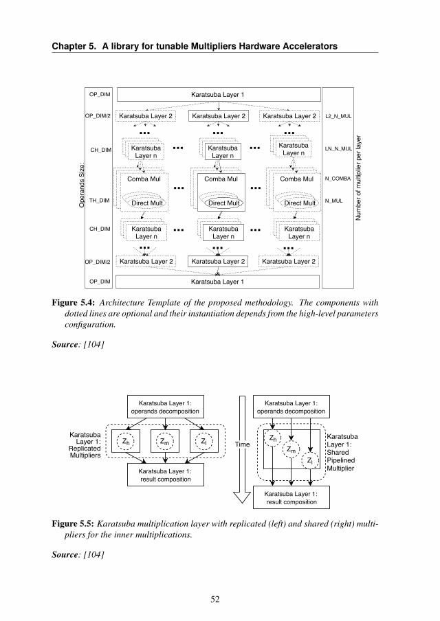
Chapter 5. A library for tunable Multipliers Hardware Accelerators
Karatsuba Layer 1
Karatsuba Layer 2
...
Karatsuba Layer 1
Karatsuba Layer 2 Karatsuba Layer 2Karatsuba Layer 2
OP_DIM
OP_DIM/2
CH_DIM
Ope
rand
s Si
ze:
TH_DIM
CH_DIM
OP_DIM/2
OP_DIM
Karatsuba Layer 2 Karatsuba Layer 2
Comba Mul
Direct Mult
...
... Comba Mul
Direct Mult
... Comba Mul
Direct Mult
... ...
...
...
...
...
... ...
KaratsubaLayer n
Num
ber o
f mul
tiplie
r per
laye
r
L2_N_MUL
LN_N_MUL
N_COMBA
N_MUL
KaratsubaLayer n
KaratsubaLayer n
KaratsubaLayer n
KaratsubaLayer n
KaratsubaLayer n
... ... ...
Figure 5.4: Architecture Template of the proposed methodology. The components withdotted lines are optional and their instantiation depends from the high-level parametersconfiguration.
Source: [104]
Time
Karatsuba Layer 1:operands decomposition
Karatsuba Layer 1: result composition
Karatsuba Layer 1: Shared Pipelined Multiplier
ZhZm
Zl
Karatsuba Layer 1:operands decomposition
Karatsuba Layer 1: result composition
Karatsuba Layer 1:
Replicated Multipliers
Zh Zm Zl
Figure 5.5: Karatsuba multiplication layer with replicated (left) and shared (right) multi-pliers for the inner multiplications.
Source: [104]
52
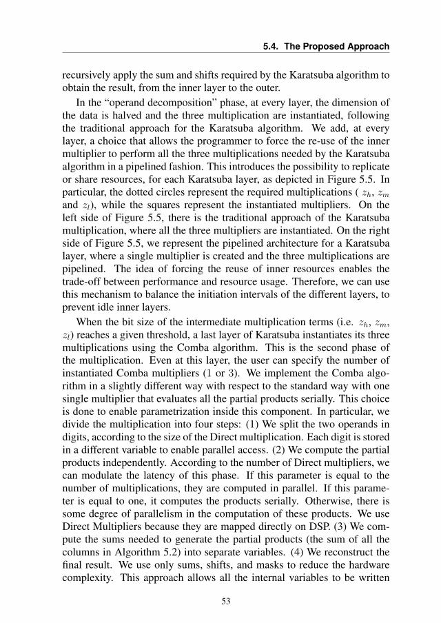
5.4. The Proposed Approach
recursively apply the sum and shifts required by the Karatsuba algorithm toobtain the result, from the inner layer to the outer.
In the “operand decomposition” phase, at every layer, the dimension ofthe data is halved and the three multiplication are instantiated, followingthe traditional approach for the Karatsuba algorithm. We add, at everylayer, a choice that allows the programmer to force the re-use of the innermultiplier to perform all the three multiplications needed by the Karatsubaalgorithm in a pipelined fashion. This introduces the possibility to replicateor share resources, for each Karatsuba layer, as depicted in Figure 5.5. Inparticular, the dotted circles represent the required multiplications ( zh, zmand zl), while the squares represent the instantiated multipliers. On theleft side of Figure 5.5, there is the traditional approach of the Karatsubamultiplication, where all the three multipliers are instantiated. On the rightside of Figure 5.5, we represent the pipelined architecture for a Karatsubalayer, where a single multiplier is created and the three multiplications arepipelined. The idea of forcing the reuse of inner resources enables thetrade-off between performance and resource usage. Therefore, we can usethis mechanism to balance the initiation intervals of the different layers, toprevent idle inner layers.
When the bit size of the intermediate multiplication terms (i.e. zh, zm,zl) reaches a given threshold, a last layer of Karatsuba instantiates its threemultiplications using the Comba algorithm. This is the second phase ofthe multiplication. Even at this layer, the user can specify the number ofinstantiated Comba multipliers (1 or 3). We implement the Comba algo-rithm in a slightly different way with respect to the standard way with onesingle multiplier that evaluates all the partial products serially. This choiceis done to enable parametrization inside this component. In particular, wedivide the multiplication into four steps: (1) We split the two operands indigits, according to the size of the Direct multiplication. Each digit is storedin a different variable to enable parallel access. (2) We compute the partialproducts independently. According to the number of Direct multipliers, wecan modulate the latency of this phase. If this parameter is equal to thenumber of multiplications, they are computed in parallel. If this parame-ter is equal to one, it computes the products serially. Otherwise, there issome degree of parallelism in the computation of these products. We useDirect Multipliers because they are mapped directly on DSP. (3) We com-pute the sums needed to generate the partial products (the sum of all thecolumns in Algorithm 5.2) into separate variables. (4) We reconstruct thefinal result. We use only sums, shifts, and masks to reduce the hardwarecomplexity. This approach allows all the internal variables to be written
53
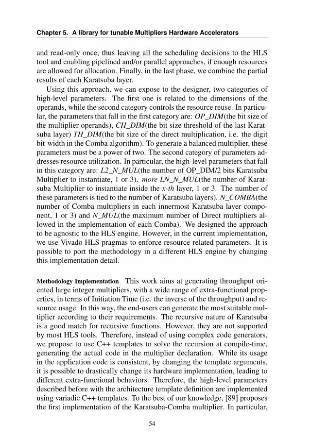
Chapter 5. A library for tunable Multipliers Hardware Accelerators
and read-only once, thus leaving all the scheduling decisions to the HLStool and enabling pipelined and/or parallel approaches, if enough resourcesare allowed for allocation. Finally, in the last phase, we combine the partialresults of each Karatsuba layer.
Using this approach, we can expose to the designer, two categories ofhigh-level parameters. The first one is related to the dimensions of theoperands, while the second category controls the resource reuse. In particu-lar, the parameters that fall in the first category are: OP_DIM(the bit size ofthe multiplier operands), CH_DIM(the bit size threshold of the last Karat-suba layer) TH_DIM(the bit size of the direct multiplication, i.e. the digitbit-width in the Comba algorithm). To generate a balanced multiplier, theseparameters must be a power of two. The second category of parameters ad-dresses resource utilization. In particular, the high-level parameters that fallin this category are: L2_N_MUL(the number of OP_DIM/2 bits KaratsubaMultiplier to instantiate, 1 or 3). more LN_N_MUL(the number of Karat-suba Multiplier to instantiate inside the x-th layer, 1 or 3. The number ofthese parameters is tied to the number of Karatsuba layers). N_COMBA(thenumber of Comba multipliers in each innermost Karatsuba layer compo-nent, 1 or 3) and N_MUL(the maximum number of Direct multipliers al-lowed in the implementation of each Comba). We designed the approachto be agnostic to the HLS engine. However, in the current implementation,we use Vivado HLS pragmas to enforce resource-related parameters. It ispossible to port the methodology in a different HLS engine by changingthis implementation detail.
Methodology Implementation This work aims at generating throughput ori-ented large integer multipliers, with a wide range of extra-functional prop-erties, in terms of Initiation Time (i.e. the inverse of the throughput) and re-source usage. In this way, the end-users can generate the most suitable mul-tiplier according to their requirements. The recursive nature of Karatsubais a good match for recursive functions. However, they are not supportedby most HLS tools. Therefore, instead of using complex code generators,we propose to use C++ templates to solve the recursion at compile-time,generating the actual code in the multiplier declaration. While its usagein the application code is consistent, by changing the template arguments,it is possible to drastically change its hardware implementation, leading todifferent extra-functional behaviors. Therefore, the high-level parametersdescribed before with the architecture template definition are implementedusing variadic C++ templates. To the best of our knowledge, [89] proposesthe first implementation of the Karatsuba-Comba multiplier. In particular,
54
5.4. The Proposed Approach
Karatsuba Layer 1: Operands Decomposition
Karatsuba Layer 1: Result Composition
Karatsuba Layer 2: Result Composition
2048
1024
512O
pera
nds
Size
:
Karatsuba Layer 2: Operands Decomposition
256
Num
ber o
f mul
tiplie
r per
laye
r
1
3
1
1
2
128
32
Karatsuba Layer 3:
Operands Decomposition
Karatsuba Layer 4:
Operands Decomposition
Karatsuba Layer 4:
Result Composition
Comba Mul
Direct Mult
Karatsuba Layer 3:
Result Composition
Karatsuba Layer 3:
Operands Decomposition
Karatsuba Layer 4:
Operands Decomposition
Karatsuba Layer 4:
Result Composition
Comba Mul
Direct Mult
Karatsuba Layer 3:
Result Composition
Karatsuba Layer 3:
Operands Decomposition
Karatsuba Layer 4:
Operands Decomposition
Karatsuba Layer 4:
Result Composition
Comba Mul
Direct Mult
Karatsuba Layer 3:
Result Composition
Figure 5.6: An example of multiplier that can be generated by the proposed approach,according the high-level parameters configuration.
it investigates a hardware design that uses a single layer of Karatsuba, toreduce the operands bit-width, and three Comba multipliers to perform theinner products. However, its implementation does not follow a pipelineapproach and it exposes limited flexibility. On the contrary, our proposedapproach is throughput oriented, and it enables a greater level of flexibilitysince it enables the reuse of pipelined components. Indeed, by changinghigh-level parameters, it is possible to set the number of Karatsuba layers.Moreover, it is possible to define for each layer the reuse policies to limitthe area of the multiplier, leading to unexplored multiplier architectures.
Figure 5.6 shows an example of a generated multiplier architecture. Wereport the operands bit-size on the left side of the image, while on the rightside we report the number of multipliers used in each layer. In particu-lar, it aims at multiplying two 2048 bit integers (OP_DIM= 2048). Thisinstance exploits 4 layers of Karatsuba to reduce the size of the operands(CH_DIM= 256). Moreover, we enforce the reuse of all the multipliers, ex-cept the ones of the third Karatsuba layer (L2_N_MUL= 1, L3_N_MUL=3, L4_N_MUL= 1, N_COMBA= 1). Finally, we use two (N_MUL= 2) 32bits (TH_DIM= 32) direct multipliers in each Comba multiplier. This mul-tiplier is declared with a single line of cpp code, where we set the param-eters in this simple way: multiplier <2048,256,32,1,2,1,3,1>(A,B,OUT),where A and B are two ap_uint<2048>and out is an ap_uint<4096>variables.The actual parametrized interface of the whole library is:
55
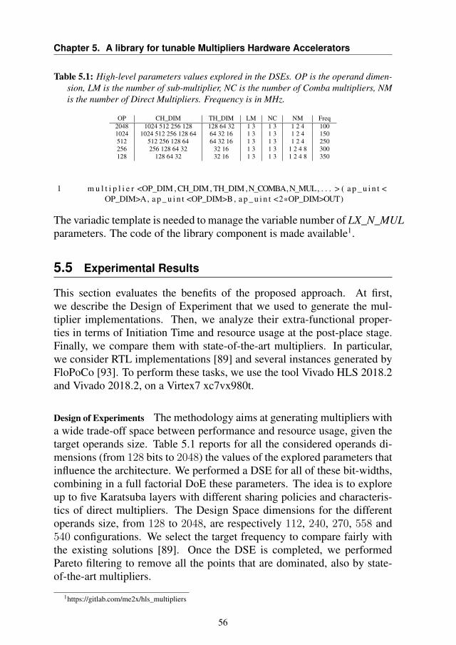
Chapter 5. A library for tunable Multipliers Hardware Accelerators
Table 5.1: High-level parameters values explored in the DSEs. OP is the operand dimen-sion, LM is the number of sub-multiplier, NC is the number of Comba multipliers, NMis the number of Direct Multipliers. Frequency is in MHz.
OP CH_DIM TH_DIM LM NC NM Freq2048 1024 512 256 128 128 64 32 1 3 1 3 1 2 4 1001024 1024 512 256 128 64 64 32 16 1 3 1 3 1 2 4 150512 512 256 128 64 64 32 16 1 3 1 3 1 2 4 250256 256 128 64 32 32 16 1 3 1 3 1 2 4 8 300128 128 64 32 32 16 1 3 1 3 1 2 4 8 350
1 m u l t i p l i e r <OP_DIM , CH_DIM, TH_DIM ,N_COMBA,N_MUL, . . . > ( a p _ u i n t <OP_DIM>A, a p _ u i n t <OP_DIM>B , a p _ u i n t <2*OP_DIM>OUT)
The variadic template is needed to manage the variable number of LX_N_MULparameters. The code of the library component is made available1.
5.5 Experimental Results
This section evaluates the benefits of the proposed approach. At first,we describe the Design of Experiment that we used to generate the mul-tiplier implementations. Then, we analyze their extra-functional proper-ties in terms of Initiation Time and resource usage at the post-place stage.Finally, we compare them with state-of-the-art multipliers. In particular,we consider RTL implementations [89] and several instances generated byFloPoCo [93]. To perform these tasks, we use the tool Vivado HLS 2018.2and Vivado 2018.2, on a Virtex7 xc7vx980t.
Design of Experiments The methodology aims at generating multipliers witha wide trade-off space between performance and resource usage, given thetarget operands size. Table 5.1 reports for all the considered operands di-mensions (from 128 bits to 2048) the values of the explored parameters thatinfluence the architecture. We performed a DSE for all of these bit-widths,combining in a full factorial DoE these parameters. The idea is to exploreup to five Karatsuba layers with different sharing policies and characteris-tics of direct multipliers. The Design Space dimensions for the differentoperands size, from 128 to 2048, are respectively 112, 240, 270, 558 and540 configurations. We select the target frequency to compare fairly withthe existing solutions [89]. Once the DSE is completed, we performedPareto filtering to remove all the points that are dominated, also by state-of-the-art multipliers.
1https://gitlab.com/me2x/hls_multipliers
56
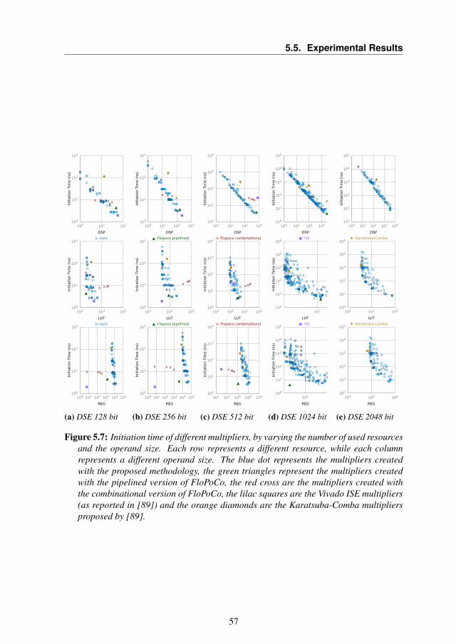
5.5. Experimental Results
Init
iati
on T
ime (
ns)
DSP
o
o
o
oo
o
o
oo
o
o
o
oo
o
oo
o
o
o
o
o
o
o
o
o
o
o
o
o
o
o
o
o
oo
o
o
oo
ooo
oo
o
o
oooo
o
o
oo
o
o
o
oo
o
ooo
oo
o
oo
o
o
xx
▲
x x
◼
◆
100
101
102
103
100 101 102
o: ours
Init
iati
on T
ime (
ns)
LUT
o
o
o
oo
o
o
oo
o
o
o
oo
o
oo
o
o
o
o
o
o
o
o
o
o
o
o
o
o
o
o
o
oo
o
o
o o
ooo
oo
o
o
oooo
o
o
oo
o
o
o
oo
o
ooo
oo
o
oo
o
o
xx
▲
xx
◼
◆
100
101
102
103
103 104 105
o: ours
Init
iati
on T
ime (
ns)
REG
o
o
o
oo
o
o
oo
o
o
o
oo
o
oo
o
o
o
o
o
o
o
o
o
o
o
o
o
o
o
o
o
oo
o
o
oo
ooo
oo
o
o
oooo
o
o
oo
o
o
o
oo
o
ooo
oo
o
oo
o
o
xx
▲
xx
◼
◆
100
101
102
103
100 101 102 103 104 105
(a) DSE 128 bit
Init
iati
on T
ime (
ns)
DSP
oo
oo
o
oo
o
o
o
oo
o
o
ooo
oo o
ooo
o
o
o
o
o
o oo
o
oo
oo
o o
o
ooo
oo
o
o
o
o
o
o
o
o
o
o
oo
oo
o
o
o
o
o
o
o
ooo
o
o
o
o
oo
o
o
o
oo
o
▲
x xx
x
◼
◆
100
101
102
103
100 101 102 103
▲: Flopoco pipelined
Init
iati
on T
ime (
ns)
LUT
oo
oo
o
o o
o
o
o
oo
o
o
oooo oo
ooo
o
o
o
o
o
ooo
o
oo
oo
oo
o
ooo
oo
o
o
o
o
o
o
o
o
o
o
oo
oo
o
o
o
o
o
o
o
ooo
o
o
o
o
oo
o
o
o
oo
o
▲
xxx
x
◼
◆
100
101
102
103
103 104 105
▲: Flopoco pipelined
Init
iati
on T
ime (
ns)
REG
oo
oo
o
oo
o
o
o
oo
o
o
oooooo
ooo
o
o
o
o
o
ooo
o
oo
oo
oo
o
ooo
oo
o
o
o
o
o
o
o
o
o
o
oo
oo
o
o
o
o
o
o
o
ooo
o
o
o
o
oo
o
o
o
oo
o
▲
x xx
x
◼
◆
100
101
102
103
100 101 102 103 104 105
(b) DSE 256 bit
Init
iati
on T
ime (
ns)
DSP
o
o
ooo
o
oo
o
oo
o
o
o
o
oo
o
o
o
o
o
o
o
o
o
oo
o
o
oo
o
oo
o
o
oo
oo
o
o
o
o
o
o
o
o
o
oo
o
o
o
oo
o
o
o
o
o
ooo
o
o
o
oo
o
oooo
o
o
o
o
o
o
o
o
oo▲
xxxx ◼
◆
100
101
102
103
104
100 101 102 103
x: Flopoco combinational
Init
iati
on T
ime (
ns)
LUT
o
o
ooo
o
o o
o
oo
o
o
o
o
oo
o
o
o
o
o
o
o
o
o
oo
o
o
oo
o
oo
o
o
oo
oo
o
o
o
o
o
o
o
o
o
oo
o
o
o
oo
o
o
o
o
o
ooo
o
o
o
oo
o
ooooo
o
o
o
o
o
o
o
oo▲
x xx x◼
◆
100
101
102
103
104
103 104 105 106
x: Flopoco combinational
Init
iati
on T
ime (
ns)
REG
o
o
ooo
o
o o
o
oo
o
o
o
o
oo
o
o
o
o
o
o
o
o
o
oo
o
o
oo
o
oo
o
o
oo
oo
o
o
o
o
o
o
o
o
o
oo
o
o
o
oo
o
o
o
o
o
ooo
o
o
o
oo
o
ooo
oo
o
o
o
o
o
o
o
oo▲
xxxx◼
◆
100
101
102
103
104
102 103 104 105 106
(c) DSE 512 bit
Init
iati
on T
ime (
ns)
DSP
o
o
o
o
o
o
o
oo
o
o
o
oo
oo
o
o
oo
o
o
o
oooo
o
oo
o
o
o
o
o
oo
o
o
o
o
oo
o
o
o
o
o
o
oo
o
o
o
oo
o
o
o
o
o
o
o
o
o
o
o
o
o
o
oo
o
ooo
o
oo
ooo
o
o
o
o
o
o
o
o
o
o
oo
o
o
o
o
o
o
ooo
oo
oo
o
o
o
o
o
o
oo
o
oo
o
o
o
o
o
o
oo
o
o
o
o
o
oo
oo
o
o
o
oo
o
o
o
o
o
o
o
o
o
o
o
o
o
o
o
ooo
o
o
o
o
o
o
o
o
o
oo
o
o
o
oo
o
o
oo
oo
o
o
o
o
oo
o
o
o
o
o
o
o
o
o
o
o
oo
o
o
o
oo
o
o
oo
o
o
o
o
o
o
o
o
o
o
o
oo
oo
o
o
o
o
o
o
o
o
oo
o
o
o
o
o
o
o
o
o
o
o
o
o
oo
o
x
▲
◆
100
101
102
103
104
105
100 101 102 103
◼: ISE
Init
iati
on T
ime (
ns)
LUT
o
o
o
o
o
o
o
oo
o
o
o
oo
oo
o
o
oo
o
o
o
oooo
o
oo
o
o
o
o
o
oo
o
o
o
o
oo
o
o
o
o
o
o
oo
o
o
o
oo
o
o
o
o
o
o
o
o
o
o
o
o
o
o
oo
o
ooo
o
oo
oo o
o
o
o
o
o
o
o
o
o
o
o o
o
o
o
o
o
o
oo o
oo
oo
o
o
o
o
o
o
oo
o
oo
o
o
o
o
o
o
oo
o
o
o
o
o
oo
oo
o
o
o
oo
o
o
o
o
o
o
o
o
o
o
o
o
o
o
o
o oo
o
o
o
o
o
o
o
o
o
o o
o
o
o
o o
o
o
oo
oo
o
o
o
o
oo
o
o
o
o
o
o
o
o
o
o
o
o o
o
o
o
oo
o
o
o o
o
o
o
o
o
o
o
o
o
o
o
oo
oo
o
o
o
o
o
o
o
o
oo
o
o
o
o
o
o
o
o
o
o
o
o
o
oo
o
x
▲
◆
100
101
102
103
104
105
105
◼: ISE
Init
iati
on T
ime (
ns)
REG
o
o
o
o
o
o
o
o o
o
o
o
oo
oo
o
o
oo
o
o
o
oooo
o
oo
o
o
o
o
o
ooo
o
o
o
o o
o
o
o
o
o
o
oo
o
o
o
oo
o
o
o
o
o
o
o
o
o
o
o
o
o
o
oo
o
ooo
o
oo
oo o
o
o
o
o
o
o
o
o
o
o
o o
o
o
o
o
o
o
oo o
oo
oo
o
o
o
o
o
o
o o
o
oo
o
o
o
o
o
o
oo
o
o
o
o
o
oo
oo
o
o
o
oo
o
o
o
o
o
o
o
o
o
o
o
o
o
o
o
o oo
o
o
o
o
o
o
o
o
o
o o
o
o
o
oo
o
o
oo
oo
o
o
o
o
oo
o
o
o
o
o
o
o
o
o
o
o
oo
o
o
o
o o
o
o
oo
o
o
o
o
o
o
o
o
o
o
o
oo
oo
o
o
o
o
o
o
o
o
oo
o
o
o
o
o
o
o
o
o
o
o
o
o
oo
o▲
◆
100
101
102
103
104
105
105
(d) DSE 1024 bit
Init
iati
on T
ime (
ns)
DSP
o
ooo
ooo
oo oo
o
o
o
o
o
o
o
o
oo
o
o
o
oo
oo
oo
o
o
o
oo
o
oo
o
o
o
o
oo
o
o
o
o
o
oo
o
o
o
oo
o
o
o
o
o
o
o
o
o
oo
oo
o
o
oo
oo
o
o
o
o
o
o
o
o
o
o
o
oo
o
oo
o
oo
o
o
o
o
o
ooo
o
o
o
◆
100
101
102
103
104
105
100 101 102 103 104
♦: Karatsuba-Comba
LUT
o
ooo
oo o
oooo
o
o
o
o
o
o
o
o
oo
o
o
o
oo
oo
oo
o
o
o
oo
o
oo
o
o
o
o
ooo
o
o
o
o
oo
o
o
o
oo
o
o
o
o
o
o
o
o
o
oo
oo
o
o
oo
o o
o
o
o
o
o
o
o
o
o
o
o
oo
o
oo
o
oo
o
o
o
o
o
o oo
o
o
o
◆
100
101
102
103
104
105
104 105 106
♦: Karatsuba-Comba
REG
o
ooo
ooo
oooo
o
o
o
o
o
o
o
o
oo
o
o
o
oo
oo
oo
o
o
o
o o
o
oo
o
o
o
o
ooo
o
o
o
o
oo
o
o
o
oo
o
o
o
o
o
o
o
o
o
oo
o o
o
o
oo
o o
o
o
o
o
o
o
o
o
o
o
o
oo
o
oo
o
oo
o
o
o
o
o
o oo
o
o
o
◆
100
101
102
103
104
105
104 105 106
(e) DSE 2048 bit
Figure 5.7: Initiation time of different multipliers, by varying the number of used resourcesand the operand size. Each row represents a different resource, while each columnrepresents a different operand size. The blue dot represents the multipliers createdwith the proposed methodology, the green triangles represent the multipliers createdwith the pipelined version of FloPoCo, the red cross are the multipliers created withthe combinational version of FloPoCo, the lilac squares are the Vivado ISE multipliers(as reported in [89]) and the orange diamonds are the Karatsuba-Comba multipliersproposed by [89].
57
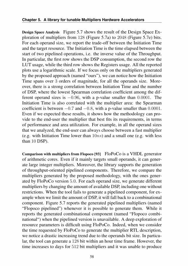
Chapter 5. A library for tunable Multipliers Hardware Accelerators
Design Space Analysis Figure 5.7 shows the result of the Design Space Ex-ploration of multipliers from 128 (Figure 5.7a) to 2048 (Figure 5.7e) bits.For each operand size, we report the trade-off between the Initiation Timeand the target resource. The Initiation Time is the time elapsed between thestart of two pipelined operations, i.e. the inverse value of the Throughput.In particular, the first row shows the DSP consumption, the second row theLUT usage, while the third row shows the Registers usage. All the reportedplots use a logarithmic scale. If we focus only on the multipliers generatedby the proposed approach (named “ours”), we can notice how the InitiationTime spans over 3 orders of magnitude, for all the operands size. More-over, there is a strong correlation between Initiation Time and the numberof DSP, where the lowest Spearman correlation coefficient among the dif-ferent operand sizes is −0.96, with a p-value smaller than 0.0001. TheInitiation Time is also correlated with the multiplier area: the Spearmancoefficient is between −0.7 and −0.8, with a p-value smaller than 0.0001.Even if we expected these results, it shows how the methodology can pro-vide to the end-user the multiplier that best fits its requirements, in termsof performance and area utilization. For example, in all the operand sizesthat we analyzed, the end-user can always choose between a fast multiplier(e.g. with Initiation Time lower than 10ns) and a small one (e.g. with lessthan 10 DSP).
Comparison with multipliers from Flopoco [93] FloPoCo is a VHDL generatorof arithmetic cores. Even if it mainly targets small operands, it can gener-ate large integer multipliers. Moreover, the library supports the generationof throughput-oriented pipelined components. Therefore, we compare themultipliers generated by the proposed methodology, with the ones gener-ated by FloPoCo version 5.0. For each operand size, we generate differentmultipliers by changing the amount of available DSP, including one withoutrestrictions. When the tool fails to generate a pipelined component, for ex-ample when we limit the amount of DSP, it will fall back to a combinationalcomponent. Figure 5.7 reports the generated pipelined multipliers (named“Flopoco pipelined”) whenever it is possible to generate them. While itreports the generated combinational component (named “Flopoco combi-national“) when the pipelined version is unavailable. A deep exploration ofresource parameters is difficult using FloPoCo. Indeed, when we considerthe time requested by FloPoCo to generate the multiplier RTL description,we notice a drastic increasing trend due to the operands bit size. In particu-lar, the tool can generate a 128 bit within an hour time frame. However, thetime increases to days for 512 bit multipliers and it was unable to produce
58
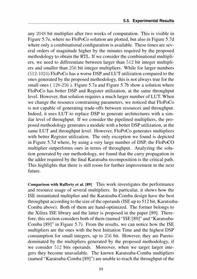
5.5. Experimental Results
any 2048 bit multiplier after two weeks of computation. This is visible inFigure 5.7e, where no FloPoCo solution are plotted, but also in Figure 5.7dwhere only a combinational configuration is available. These times are sev-eral orders of magnitude higher by the minutes required by the proposedmethodology to obtain the RTL. If we consider the combinational multipli-ers, we need to differentiate between larger than 512 bit integer multipli-ers and smaller than 256 bit integer multipliers. While for larger numbers(512-1024) FloPoCo has a worse DSP and LUT utilization compared to theones generated by the proposed methodology, this is not always true for thesmall ones ( 128-256 ). Figure 5.7a and Figure 5.7b show a solution whereFloPoCo has better DSP and Register utilization, at the same throughputlevel. However, that solution requires a much larger number of LUT. Whenwe change the resource constraining parameters, we noticed that FloPoCois not capable of generating trade-offs between resources and throughput.Indeed, it uses LUT to replace DSP to generate architectures with a sim-ilar level of throughput. If we consider the pipelined multipliers, the pro-posed methodology generates a module with a better DSP utilization, at thesame LUT and throughput level. However, FloPoCo generates multiplierswith better Register utilization. The only exception we found is depictedin Figure 5.7d where, by using a very large number of DSP, the FloPoCOmultiplier outperforms ours in terms of throughput. Analyzing the solu-tion generated by our methodology, we found that the carry propagation inthe adder required by the final Karatsuba recomposition is the critical path.This highlights that there is still room for further improvement in the nextfuture.
Comparison with Rafferty et al. [89] This work investigates the performanceand resource usage of several multipliers. In particular, it shows how theISE instantiated multiplier and the Karatsuba-Comba design have the bestthroughput according to the size of the operands (ISE up to 512 bit, Karatsuba-Comba above). Both of them are hand-optimized. The former belongs tothe Xilinx ISE library and the latter is proposed in the paper [89]. There-fore, this section considers both of them (named “ISE [89]” and “Karatsuba-Comba [89]” in Figure 5.7). From the results, we can notice how the ISEmultipliers are the ones with the best Initiation Time and the highest DSPconsumption for small integers, up to 256 bit. However, they are Pareto-dominated by the multipliers generated by the proposed methodology, ifwe consider 512 bits operands. Moreover, when we target larger inte-gers they become unavailable. The known Karatsuba-Comba multipliers(named “Karatsuba-Comba [89]”) are unable to reach the throughput of the
59
Chapter 5. A library for tunable Multipliers Hardware Accelerators
multipliers generated by the proposed methodology, with the same amountof DSP, for all the analyzed bit sizes. However, we can notice that thehand-designed hardware can efficiently use LUT and Registers, comparedto other multipliers that target a similar throughput. This behavior is due tothe HLS procedure that is unable to reach the same optimization level whenit translates high-level languages into hardware description. Both the solu-tions presented in [89] are not flexible and do not allow any performance-resource trade-off exploration.
5.6 Summary
Working with FPGA increases the complexity of evaluating the performance-power tradeoffs that the developer needs to consider when writing applica-tions. In this chapter, we have seen a methodology that allows generatinga tunable library of large integer multipliers using HLS. It uses a para-metric Karatsuba-Comba multiplication template to instantiate throughputoriented multipliers. This flexibility enables the end-user to select the mostsuitable multiplier, according to the application requirements, after havingevaluated the possible trade-offs. Indeed, from experimental results, wecan notice how the proposed methodology can generate multipliers with arange of performances and resource usage that is greater than one order ofmagnitude.
The outcome of this work has been published in the Design, Automationand Test in Europe Conference, 2021 [104].
60
CHAPTER6Autotuning a Server-Side Car Navigation
System
In this chapter, we study a HPC application and we try to improve the com-putation efficiency of this application by searching for a proactive way tolimit the amount of computation required. In particular, we analyze a Prob-abilistic Time-Dependent Routing application (PTDR), a component in atraffic navigator application. We propose a novel approach for dynamicallyselecting the number of samples used for the Monte Carlo simulation thatis used to solve the PTDR, thus improving the computation efficiency. Thefocal point of this approach is the study of the input and the research of afunction that can extract characteristics of the input that can be used to drivethe application. Once this function is found, we integrate it into the orig-inal application with the LARA aspect-oriented language, already used inChapter 4 for a different purpose. We manage the runtime process of selec-tion with mARGOt autotuner, which has been enriched with the proactivefunctionality thanks to this case study.
61
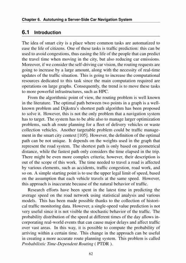
Chapter 6. Autotuning a Server-Side Car Navigation System
6.1 Introduction
The idea of smart city is a place where common tasks are automatized toease the life of citizens. One of these tasks is traffic prediction: this can beused to avoid congestions, thus easing the life of the people that can predictthe travel time when moving in the city, but also reducing car emissions.Moreover, if we consider the self-driving car vision, the routing requests aregoing to increase by a large amount, along with the necessity of real-timeupdates of the traffic situation. This is going to increase the computationalresources dedicated to this task since the main computation required areoperations on large graphs. Consequently, the trend is to move these tasksto more powerful infrastructures, such as HPC.
From the algorithmic point of view, the routing problem is well knownin the literature. The optimal path between two points in a graph is a well-known problem and Dijkstra’s shortest path algorithm has been proposedto solve it. However, this is not the only problem that a navigation systemhas to target. The system has to be able also to manage larger optimizationproblems, such ah route planning for a fleet of delivery vehicles or wastecollection vehicles. Another targetable problem could be traffic manage-ment in the smart city context [105]. However, the definition of the optimalpath can be not unique. It depends on the weights used in the graph thatrepresent the road system. The shortest path is only based on geometricaldistance, while the fastest path only considers the time elapsed in the trip.There might be even more complex criteria; however, their description isout of the scope of this work. The time needed to travel a road is affectedby various elements, such as accidents, traffic congestion, road work, andso on. A simple starting point is to use the upper legal limit of speed, basedon the assumption that each vehicle travels at the same speed. However,this approach is inaccurate because of the natural behavior of traffic.
Research efforts have been spent in the latest time in predicting theaverage speed on the road network using statistical analysis and variousmodels. This has been made possible thanks to the collection of histori-cal traffic monitoring data. However, a single-speed value prediction is notvery useful since it is not visible the stochastic behavior of the traffic. Theprobability distribution of the speed at different times of the day allows in-corporating real-world events that can cause major delays and affect trafficover vast areas. In this way, it is possible to compute the probability ofarriving within a certain time. This change in the approach can be usefulin creating a more accurate route planning system. This problem is calledProbabilistic Time-Dependent Routing ( PTDR ).
62
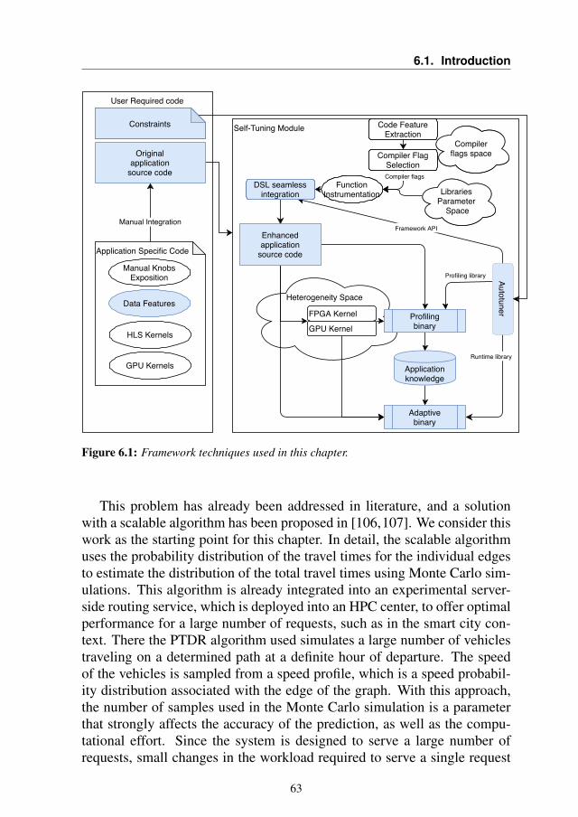
6.1. Introduction
User Required code
Self-Tuning Module
Heterogeneity Space
Originalapplication
source code
Code FeatureExtraction
Compilerflags space
Compiler flags
Compiler FlagSelection
Libraries Parameter
Space
DSL seamlessintegration
Enhancedapplication
source code
Profilingbinary
Applicationknowledge
Adaptivebinary
Runtime library
Framework API
Autotuner
Profiling library
Manual Integration
Application Specific Code
Data Features
HLS Kernels
GPU Kernels
FPGA Kernel
GPU Kernel
Constraints
Manual KnobsExposition
FunctionInstrumentation
Constraints Code FeatureExtraction
Compiler FlagSelection
FunctionInstrumentation Libraries
Parameter Space
Compilerflags space
DSL seamlessintegration
Autotuner
Figure 6.1: Framework techniques used in this chapter.
This problem has already been addressed in literature, and a solutionwith a scalable algorithm has been proposed in [106,107]. We consider thiswork as the starting point for this chapter. In detail, the scalable algorithmuses the probability distribution of the travel times for the individual edgesto estimate the distribution of the total travel times using Monte Carlo sim-ulations. This algorithm is already integrated into an experimental server-side routing service, which is deployed into an HPC center, to offer optimalperformance for a large number of requests, such as in the smart city con-text. There the PTDR algorithm used simulates a large number of vehiclestraveling on a determined path at a definite hour of departure. The speedof the vehicles is sampled from a speed profile, which is a speed probabil-ity distribution associated with the edge of the graph. With this approach,the number of samples used in the Monte Carlo simulation is a parameterthat strongly affects the accuracy of the prediction, as well as the compu-tational effort. Since the system is designed to serve a large number ofrequests, small changes in the workload required to serve a single request
63
Chapter 6. Autotuning a Server-Side Car Navigation System
can affect the overall efficiency. The original version [106] is based on aworst-case tuning of the required number of samples, without any capabil-ity of adapting to the road or the starting time. A reactive approach likethe one suggested in [108] is not viable, thanks to its high overhead, wepropose a methodology to proactively select the number of samples to usein the Monte Carlo simulation required for the PTDR algorithm.
In the context of the global framework, this chapter introduces the con-cept of data features. We define as data feature some characteristics of theinput that can be captured with a quick function before the run of the ker-nel and that can drive the run to obtain benefits from the extra-functionalpoint of view. Figure 6.1 shows the involved components, which in thiscircumstance are only the autotuning framework and some custom writ-ten functionalities to extract the data features. These functions are thenintegrated, together with the autotuner, with the DSL seamless integrationprocess to enforce the separation of concern between the functional and theextra-functional code.
In particular, the contributions of this chapter can be summarised as fol-lows:
• A methodology has been proposed to proactively self-adapt the PTDRalgorithm presented in [106, 107] to the input data;
• A probabilistic error model has been studied to correlate the charac-teristics of the input data to the number of samples used in the MonteCarlo simulation;
• An aspect-oriented programming language has been used to separatethe functional version of the application from the adaptivity layer.
6.2 Background
Many formulations of the problem of determining the optimal path in astochastic time-dependent graph have been proposed [109]. The startingpoint of this work is closest to the Shortest-path problem with on-time ar-rival reliability (SPOTAR) formulation. This is a variant of the Stochasticon-time arrival (SOTA) problem, which has a practical solution as shownin [110]. The objective of these algorithms is to maximize the probabil-ity of arriving within a time budget and can handle optimal routing in astochastic network. However, they are not able to manage time-dependentsolutions. In [109] there is a practical result for a time-dependent SOTAapproach. [111] approach the SPOTAR problem from the theoretical point
64
6.2. Background
of view, and suggests a way to extend it with time dependency. Other worksshow different theoretical approaches and practical application of the SOTAproblem [110, 112–114]. In particular, the last work [113] presents a solu-tion for the SPOTAR problem as a heuristic based on a policy-based SOTAapproach. However, the authors assume the network as time-invariant,which is not true if we consider long travels. Moreover, this solution isnot usable in on-line systems since the scalability to real-world graph is aconcerning issue.
This chapter proposes an approach that is built on top of [106, 107],where an approximate solution of the time-dependent variant of the SPOTARproblem based on Monte Carlo simulations is proposed. Our approach isbased on the k-shortest paths algorithm [115–117] to determine the pathsto use for the PTDR estimation. This separation allows us to implement thewhole approach in an online HPC system that can provide adaptive routingin real-time. Since the PTDR is based on Monte Carlo techniques, we canfind in literature some methodologies to improve its efficiency. As reportedin [118], there are two main ways to improve it. The first one is to improvethe sampling efficiency, the second is to target the sampling convergence.However, in both cases, the optimal solution is reached by exploiting theiterative nature of the Monte Carlo simulation. Indeed, several techniqueshave been proposed to determine which is the best next sample to maximizethe gathered knowledge [118, 119] thus improving the sampling efficiency.However, in the implementation under analysis, this approach is not validsince it requires analyzing the result at each sampling iteration, while wewant to exploit the parallelism of the underlying HPC architecture [107]that excludes any iterative approach to the Monte Carlo. For the same rea-son, we have to discard also the approaches that require a statistical prop-erty evaluation after every iteration. For example, [108] check the erroracceptability after every sample, which is not acceptable for our approach.Both approaches would introduce too much overhead. As already analyzedin [106], the specific problem requires that the number of samples is chosena priori in a proactive rather than in a reactive manner.
A solution closer to the proposed one has been envisioned in [120], witha two-step approach. The authors suggest having a first shot with a reducednumber of samples to provide an initial approximate solution as fast as pos-sible, and then to refine it to the required accuracy in successive iterations.In our context, this idea suffers from two big weaknesses. First, the ap-proximate result is suitable for scientific workflows where it can be used totrigger the next stage of computations, which is not our case. Second, inthe iterative phase, it uses a reactive approach that we already discussed is
65
Chapter 6. Autotuning a Server-Side Car Navigation System
not ideal in our case, since we require a proactive solution in this specificproblem to exploit HPC capabilities.
6.3 Monte Carlo Approach for Probabilistic Time-DependentRouting
Many theoretical formulations and several algorithms have been developedto solve the problem of computing the distribution of the travel times of aroad [109]. In this chapter, we consider a path-based approach (SPOTAR)where the paths are known a-priori (since they are evaluated in the pre-vious K alternative paths step) and the goal is to evaluate the travel-timedistributions for each one of those paths [121].
The complete traffic navigator application pipeline is shown in Fig-ure 6.2. The focus of this chapter is on the efficient estimation of the arrivaltime distribution (PTDR - Probabilistic Time-Dependent Routing phase).To provide a global view of the traffic navigator pipeline, the three mainsteps of the application can be described as follows:
1. Determinate the K-alternative paths. In this scenario getting the short-est path is not sufficient when no traffic information is inserted inthe road computation. For this reason, we need to evaluate morethan one road using a K-shortest path with limited overlap algorithm[115–117]. This step is out of the scope of this thesis.
2. For every path, evaluate the travel time using the PTDR module. Theexact solution of the travel time estimation has exponential complex-ity, which is approximated with the Monte Carlo approach proposedin [106]. This module is the focus of this chapter, which aims at opti-mizing the Monte Carlo simulation used in the PTDR algorithm.
3. This last step gathers all the predicted times, and reorders all themeasured paths, according to the timing distributions and user pref-erence [122].
The need for performance pushes us to implement this pipeline in an HPCsystem. Moreover, we focus on improving the performances by not doinguseless computation, following the approximate computing paradigm. Thisapproach is designed to be used in an online system to serve a large volumeof routing requests.
The definition of a probabilistic road network is inspired by the defini-tion of the stochastic time-dependent network described by Miller-Hooks[121]. The only difference is in the conception of the segment travel times,
66
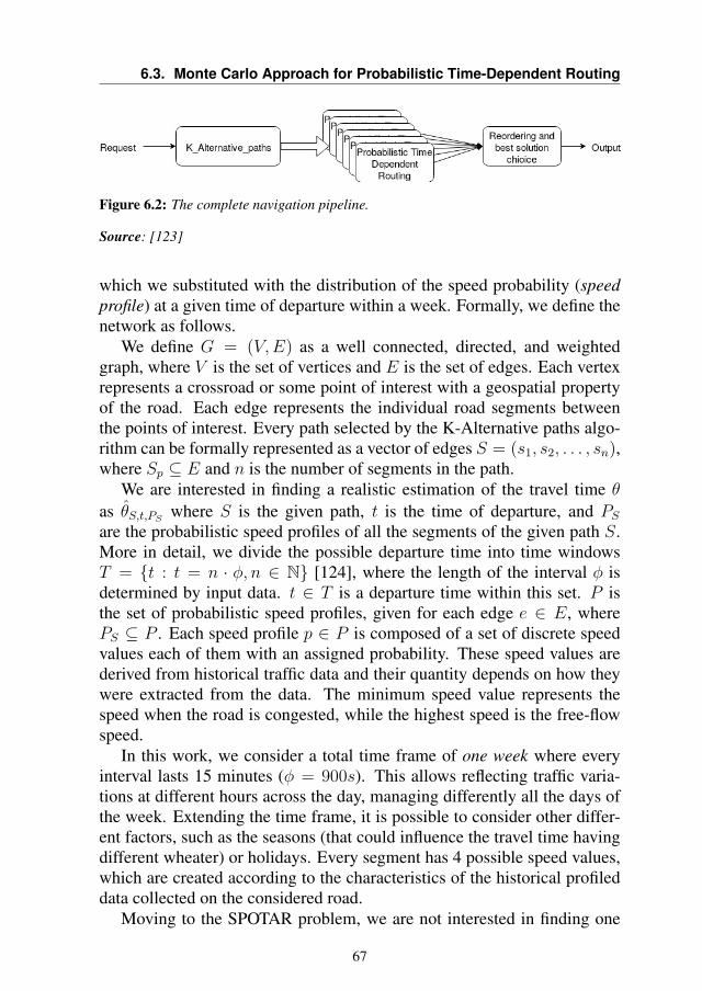
6.3. Monte Carlo Approach for Probabilistic Time-Dependent Routing
Figure 6.2: The complete navigation pipeline.
Source: [123]
which we substituted with the distribution of the speed probability (speedprofile) at a given time of departure within a week. Formally, we define thenetwork as follows.
We define G = (V,E) as a well connected, directed, and weightedgraph, where V is the set of vertices and E is the set of edges. Each vertexrepresents a crossroad or some point of interest with a geospatial propertyof the road. Each edge represents the individual road segments betweenthe points of interest. Every path selected by the K-Alternative paths algo-rithm can be formally represented as a vector of edges S = (s1, s2, . . . , sn),where Sp ⊆ E and n is the number of segments in the path.
We are interested in finding a realistic estimation of the travel time θas θS,t,PS where S is the given path, t is the time of departure, and PSare the probabilistic speed profiles of all the segments of the given path S.More in detail, we divide the possible departure time into time windowsT = {t : t = n · φ, n ∈ N} [124], where the length of the interval φ isdetermined by input data. t ∈ T is a departure time within this set. P isthe set of probabilistic speed profiles, given for each edge e ∈ E, wherePS ⊆ P . Each speed profile p ∈ P is composed of a set of discrete speedvalues each of them with an assigned probability. These speed values arederived from historical traffic data and their quantity depends on how theywere extracted from the data. The minimum speed value represents thespeed when the road is congested, while the highest speed is the free-flowspeed.
In this work, we consider a total time frame of one week where everyinterval lasts 15 minutes (φ = 900s). This allows reflecting traffic varia-tions at different hours across the day, managing differently all the days ofthe week. Extending the time frame, it is possible to consider other differ-ent factors, such as the seasons (that could influence the travel time havingdifferent wheater) or holidays. Every segment has 4 possible speed values,which are created according to the characteristics of the historical profileddata collected on the considered road.
Moving to the SPOTAR problem, we are not interested in finding one
67
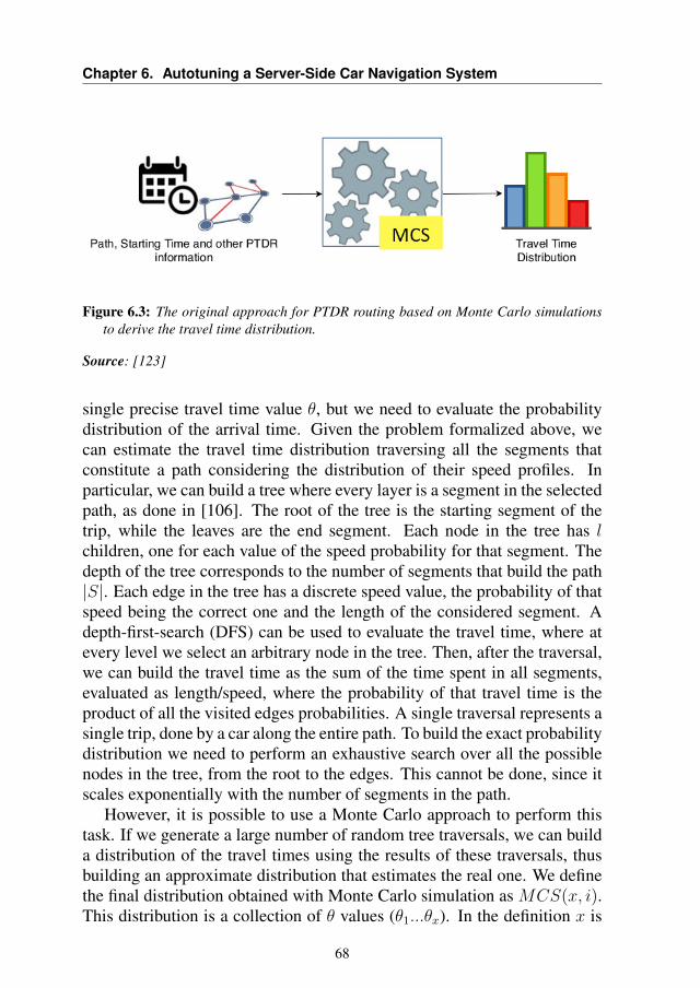
Chapter 6. Autotuning a Server-Side Car Navigation System
Figure 6.3: The original approach for PTDR routing based on Monte Carlo simulationsto derive the travel time distribution.
Source: [123]
single precise travel time value θ, but we need to evaluate the probabilitydistribution of the arrival time. Given the problem formalized above, wecan estimate the travel time distribution traversing all the segments thatconstitute a path considering the distribution of their speed profiles. Inparticular, we can build a tree where every layer is a segment in the selectedpath, as done in [106]. The root of the tree is the starting segment of thetrip, while the leaves are the end segment. Each node in the tree has lchildren, one for each value of the speed probability for that segment. Thedepth of the tree corresponds to the number of segments that build the path|S|. Each edge in the tree has a discrete speed value, the probability of thatspeed being the correct one and the length of the considered segment. Adepth-first-search (DFS) can be used to evaluate the travel time, where atevery level we select an arbitrary node in the tree. Then, after the traversal,we can build the travel time as the sum of the time spent in all segments,evaluated as length/speed, where the probability of that travel time is theproduct of all the visited edges probabilities. A single traversal represents asingle trip, done by a car along the entire path. To build the exact probabilitydistribution we need to perform an exhaustive search over all the possiblenodes in the tree, from the root to the edges. This cannot be done, since itscales exponentially with the number of segments in the path.
However, it is possible to use a Monte Carlo approach to perform thistask. If we generate a large number of random tree traversals, we can builda distribution of the travel times using the results of these traversals, thusbuilding an approximate distribution that estimates the real one. We definethe final distribution obtained with Monte Carlo simulation as MCS(x, i).This distribution is a collection of θ values (θ1...θx). In the definition x is
68
6.4. The Proposed Approach
the number of random tree traversals, and i is the input set of the θ function(i.e. S, t, PS).
These distributions usually have a long-tailed shape, because of proper-ties of the traffic such as accidents, which are rare events but have a strongimpact on the travel time. For this reason, to estimate correctly the distribu-tion of the travel times, large numbers of samples (x) are needed. As we al-ready mentioned, we cannot rely on run-time stability analysis of the MonteCarlo simulation, since we target parallel architectures we need that everysample θ of the Monte Carlo simulation, which means each tree traversal,has to be independent of the others. However, we need to know beforehandthe number of samples θ required to build the probability distribution, toefficiently exploit the parallelism.
To summarise, Figure 6.3 represent the original PTDR algorithm. Allthe required data (such as starting and ending point and starting time) aregiven to the Monte Carlo simulation, which can provide the probability dis-tribution for the given route thanks to a fixed a-priori number of traversals.
6.4 The Proposed Approach
The considered Monte Carlo simulation uses a fixed number of samples x inall the performed run. This is the conventional approach, where this numberis selected with worst-case analysis. Indeed, this is the lowest number ofsamples required to guarantee a target accuracy [107]. Here we present atechnique that we propose, which allows selecting at runtime the number ofsamples needed for the Monte Carlo simulation to guarantee the accuracyaccording to characteristics of the input data.
However, before moving to the proposed methodology, we want to prop-erly contextualize the problem. Even if we are trying to build the traveltime distribution, what we are really interested in is to know a value, τi,that guarantees that the travel time will be within that value: P (θ < τi) ≥ ywhere i is the input set of the travel-time function and y is the probabilityvalue. This value, τi, is the output of the PTDR. To enable our approxi-mation, we need to characterize this value with an additional property, y,where y is the probability that the travel time will be lower than τ . Theresulting formulation of this property is τi,y.
With the Monte Carlo simulation, we can evaluate the value of τi,y usingx samples as follows τxi,y = MCS(x, i, y). In particular, the value τxi,y isobtained selecting the y-th percentile of the distribution obtained from theMonte Carlo simulation on a finite number of samples (i.e. if y = 95% thenτxi,y is the 95th percentile of the distribution).
69
Chapter 6. Autotuning a Server-Side Car Navigation System
With the proposed approach, we want to minimize the execution timeof the MCS, while minimizing the prediction error defined as errorxi,y =|τi,y−τxi,y |
τi,y. The target problem can be expressed as follows:
minimizex
cpu_timexi
subject to errorxi,y ≤ ε(6.1)
where ε is the maximum tolerated error that can be done in the computa-tion. We want to link this error to the output of the MCS, in particular tothe desired percentile of the predicted travel time. This allows us to abstractfrom the actual path. Since there is a strong correlation between the execu-tion time and the used number of samples x, it is possible to simplify theproblem as a minimization of the number of samples x instead of cpu_timeConsidering the properties of the Monte Carlo approach, we can derive thatτi,y ≡ τ∞i,y, where τ∞i,y is the output of the MCS function when evaluatedwith an infinite number of samples. Thus, we can rewrite the error as
errorxi,y =|τ∞i,y − τxi,y|
τ∞i,y(6.2)
Another property of Monte Carlo is that the value τxi,y is a random variable,asymptotically normally distributed with mean µτxi,y and standard deviationστxi,y [125]. Then, thanks to the central limit theorem [126], if we considera number of samples high enough, the average value does not depend onthe number of Monte Carlo simulations. Moreover, the standard deviationdecreases constantly while we increase the number of samples used in theMonte Carlo simulation. Given all of these properties, it is possible todefine the error as a random variable characterized by a normal distributionwith mean 0 and a standard deviation στxi,y/µτxi,y . In the following, we refer
to the standard deviation of the error as ντxi,y =στxi,y
µτxi,y
. This is defined as
the coefficient of variation (relative standard deviation) of the result of theMonte Carlo simulation.
However, given the probabilistic nature of the problem, it is impossibleto guarantee that the error will always be below ε. On the other hand, itis possible to relax the problem by introducing the concept of confidenceinterval (CI) on the error. In particular, thanks to the normal distribution ofthe error, we can correlate the selected confidence interval with the expectederror:
P (errorxi,y ≤ ε) ≥ CI =⇒ ˆerrorxi,y ≤ n(CI)× ντxi,y ≤ ε (6.3)
70
6.4. The Proposed Approach
where n(CI) is a value that express the confidence level. We derived theconfidence level from the 1-3 σ-intervals of the normal distribution, son(68%)=1, n(95%)=2 and n(99.7%)=3. Thus, by decreasing the numberof Monte Carlo simulations used to derive τxi,y, on the one hand, we reducethe application execution time, but on the other hand we are also affect-ing the accuracy, which can be seen from the increase of the coefficient ofvariation ντxi,y .
An additional problem comes from the input dependency of τxi,y. Thismeans that, if the input is unknown (such as an unknown path) it is notpossible to predict the possible Monte Carlo error, using only the number ofsamples as prediction variable. To deal with this, we need to find a featureui of the inputs i that can be used to quickly evaluate the input and find thenumber of samples necessary to contain the error below the threshold ε. Inthis way, we can evaluate the error using ui instead of the real value i thustransforming the original problem into
errorxi,y ≤ n(CI)× ντxui,y . (6.4)
We found this feature ui , which we called unpredictability, since it rep-resents a set of characteristics of the inputs i (road, starting time,...) thatprovides information about how complex is the prediction of τi,y. There-fore this unpredictability is also related to the number of samples requiredto ensure a confidence level on the error The details on the unpredictabilityfeature and the function used to evaluate it are presented in Section 6.4.1.
With this new formulation of the problem, the error is no more directlyrelated to the specific input set i but only to the identified feature ui. Thus,the number of samples needed to satisfy the constraint on the confidencecan be extracted by ντxui,y ≤
εn(CI)
. The missing step to finalize the method-ology is to determine the correlation between the unpredictability functionand the output error. This has been done running a profiling phase on arepresentative set of inputs, to extract the values of ντxui,y that we then usedto evaluate the correlation. The details on this profiling campaign are pre-sented in Section 6.4.2
To summarise, Figure 6.4 shows the proposed methodology. We add anadaptivity layer on top of the Monte Carlo simulation to quickly determine,at runtime, from the characteristics of the actual input, the number of sam-ples required to satisfy the accuracy requirement. This is possible thanksto the feature-extraction procedure that estimates the unpredictability giventhe input data. The dynamic autotuner combines the data feature with theprofiled knowledge plus the extra-functional requirements to correctly con-figure the Monte Carlo simulation before its run.
71
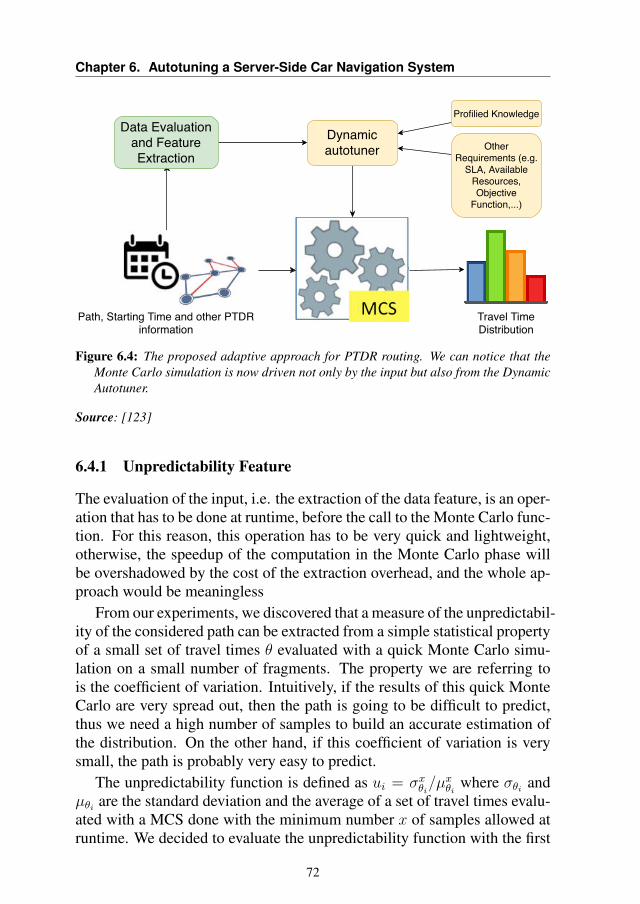
Chapter 6. Autotuning a Server-Side Car Navigation System
Path, Starting Time and other PTDRinformation
Data Evaluationand FeatureExtraction
Dynamicautotuner Other
Requirements (e.g.SLA, Available
Resources,Objective
Function,...)
Profilied Knowledge
Travel TimeDistribution
Figure 6.4: The proposed adaptive approach for PTDR routing. We can notice that theMonte Carlo simulation is now driven not only by the input but also from the DynamicAutotuner.
Source: [123]
6.4.1 Unpredictability Feature
The evaluation of the input, i.e. the extraction of the data feature, is an oper-ation that has to be done at runtime, before the call to the Monte Carlo func-tion. For this reason, this operation has to be very quick and lightweight,otherwise, the speedup of the computation in the Monte Carlo phase willbe overshadowed by the cost of the extraction overhead, and the whole ap-proach would be meaningless
From our experiments, we discovered that a measure of the unpredictabil-ity of the considered path can be extracted from a simple statistical propertyof a small set of travel times θ evaluated with a quick Monte Carlo simu-lation on a small number of fragments. The property we are referring tois the coefficient of variation. Intuitively, if the results of this quick MonteCarlo are very spread out, then the path is going to be difficult to predict,thus we need a high number of samples to build an accurate estimation ofthe distribution. On the other hand, if this coefficient of variation is verysmall, the path is probably very easy to predict.
The unpredictability function is defined as ui = σxθi/µxθi
where σθi andµθi are the standard deviation and the average of a set of travel times evalu-ated with a MCS done with the minimum number x of samples allowed atruntime. We decided to evaluate the unpredictability function with the first
72
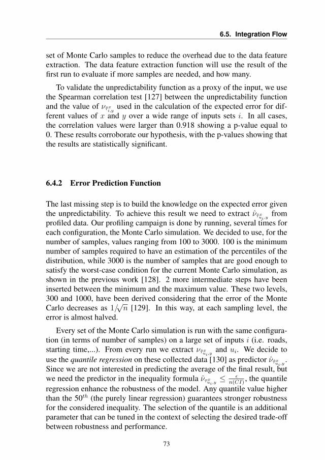
6.5. Integration Flow
set of Monte Carlo samples to reduce the overhead due to the data featureextraction. The data feature extraction function will use the result of thefirst run to evaluate if more samples are needed, and how many.
To validate the unpredictability function as a proxy of the input, we usethe Spearman correlation test [127] between the unpredictability functionand the value of ντxi,y used in the calculation of the expected error for dif-ferent values of x and y over a wide range of inputs sets i. In all cases,the correlation values were larger than 0.918 showing a p-value equal to0. These results corroborate our hypothesis, with the p-values showing thatthe results are statistically significant.
6.4.2 Error Prediction Function
The last missing step is to build the knowledge on the expected error giventhe unpredictability. To achieve this result we need to extract ντxui,y fromprofiled data. Our profiling campaign is done by running, several times foreach configuration, the Monte Carlo simulation. We decided to use, for thenumber of samples, values ranging from 100 to 3000. 100 is the minimumnumber of samples required to have an estimation of the percentiles of thedistribution, while 3000 is the number of samples that are good enough tosatisfy the worst-case condition for the current Monte Carlo simulation, asshown in the previous work [128]. 2 more intermediate steps have beeninserted between the minimum and the maximum value. These two levels,300 and 1000, have been derived considering that the error of the MonteCarlo decreases as 1/
√n [129]. In this way, at each sampling level, the
error is almost halved.
Every set of the Monte Carlo simulation is run with the same configura-tion (in terms of number of samples) on a large set of inputs i (i.e. roads,starting time,...). From every run we extract ντxui,y and ui. We decide touse the quantile regression on these collected data [130] as predictor ντxui,y .Since we are not interested in predicting the average of the final result, butwe need the predictor in the inequality formula ντxui,y ≤
εn(CI)
, the quantileregression enhance the robustness of the model. Any quantile value higherthan the 50th (the purely linear regression) guarantees stronger robustnessfor the considered inequality. The selection of the quantile is an additionalparameter that can be tuned in the context of selecting the desired trade-offbetween robustness and performance.
73
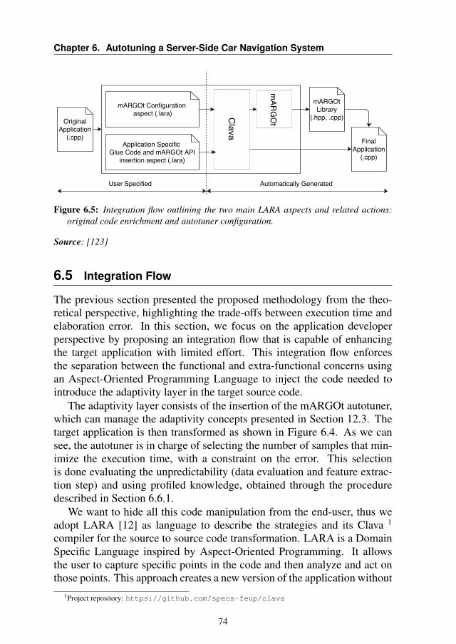
Chapter 6. Autotuning a Server-Side Car Navigation System
Clava
OriginalApplication
(.cpp) FinalApplication
(.cpp)
mARGOtLibrary
(.hpp, .cpp)
mARGOt Configuration aspect (.lara)
Application Specific Glue Code and mARGOt API
insertion aspect (.lara)
mAR
GOt
User Specified Automatically Generated
Figure 6.5: Integration flow outlining the two main LARA aspects and related actions:original code enrichment and autotuner configuration.
Source: [123]
6.5 Integration Flow
The previous section presented the proposed methodology from the theo-retical perspective, highlighting the trade-offs between execution time andelaboration error. In this section, we focus on the application developerperspective by proposing an integration flow that is capable of enhancingthe target application with limited effort. This integration flow enforcesthe separation between the functional and extra-functional concerns usingan Aspect-Oriented Programming Language to inject the code needed tointroduce the adaptivity layer in the target source code.
The adaptivity layer consists of the insertion of the mARGOt autotuner,which can manage the adaptivity concepts presented in Section 12.3. Thetarget application is then transformed as shown in Figure 6.4. As we cansee, the autotuner is in charge of selecting the number of samples that min-imize the execution time, with a constraint on the error. This selectionis done evaluating the unpredictability (data evaluation and feature extrac-tion step) and using profiled knowledge, obtained through the proceduredescribed in Section 6.6.1.
We want to hide all this code manipulation from the end-user, thus weadopt LARA [12] as language to describe the strategies and its Clava 1
compiler for the source to source code transformation. LARA is a DomainSpecific Language inspired by Aspect-Oriented Programming. It allowsthe user to capture specific points in the code and then analyze and act onthose points. This approach creates a new version of the application without
1Project repository: https://github.com/specs-feup/clava
74
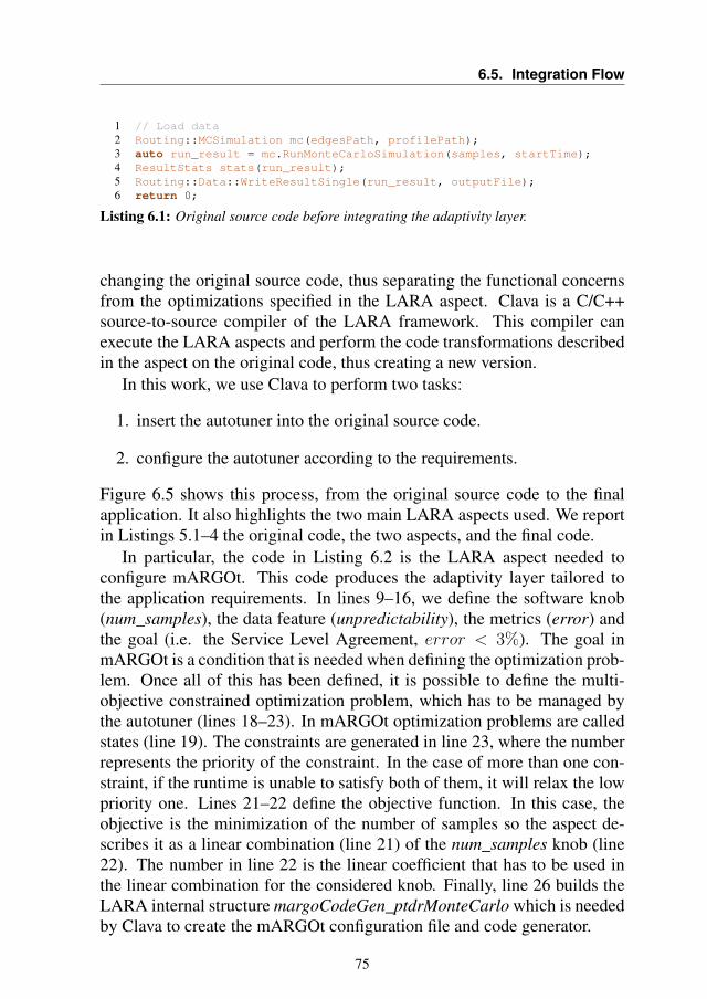
6.5. Integration Flow
1 // Load data2 Routing::MCSimulation mc(edgesPath, profilePath);3 auto run_result = mc.RunMonteCarloSimulation(samples, startTime);4 ResultStats stats(run_result);5 Routing::Data::WriteResultSingle(run_result, outputFile);6 return 0;
Listing 6.1: Original source code before integrating the adaptivity layer.
changing the original source code, thus separating the functional concernsfrom the optimizations specified in the LARA aspect. Clava is a C/C++source-to-source compiler of the LARA framework. This compiler canexecute the LARA aspects and perform the code transformations describedin the aspect on the original code, thus creating a new version.
In this work, we use Clava to perform two tasks:
1. insert the autotuner into the original source code.
2. configure the autotuner according to the requirements.
Figure 6.5 shows this process, from the original source code to the finalapplication. It also highlights the two main LARA aspects used. We reportin Listings 5.1–4 the original code, the two aspects, and the final code.
In particular, the code in Listing 6.2 is the LARA aspect needed toconfigure mARGOt. This code produces the adaptivity layer tailored tothe application requirements. In lines 9–16, we define the software knob(num_samples), the data feature (unpredictability), the metrics (error) andthe goal (i.e. the Service Level Agreement, error < 3%). The goal inmARGOt is a condition that is needed when defining the optimization prob-lem. Once all of this has been defined, it is possible to define the multi-objective constrained optimization problem, which has to be managed bythe autotuner (lines 18–23). In mARGOt optimization problems are calledstates (line 19). The constraints are generated in line 23, where the numberrepresents the priority of the constraint. In the case of more than one con-straint, if the runtime is unable to satisfy both of them, it will relax the lowpriority one. Lines 21–22 define the objective function. In this case, theobjective is the minimization of the number of samples so the aspect de-scribes it as a linear combination (line 21) of the num_samples knob (line22). The number in line 22 is the linear coefficient that has to be used inthe linear combination for the considered knob. Finally, line 26 builds theLARA internal structure margoCodeGen_ptdrMonteCarlo which is neededby Clava to create the mARGOt configuration file and code generator.
75
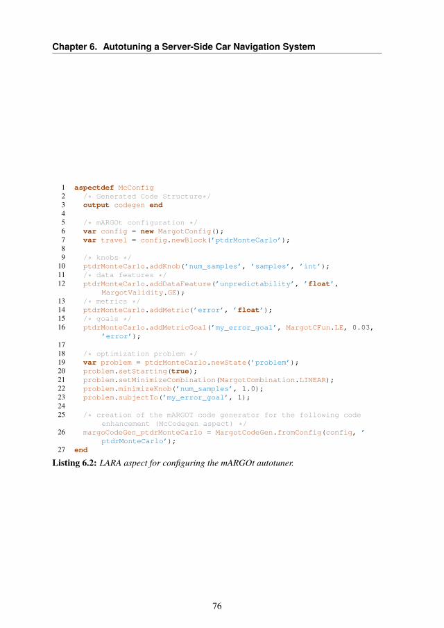
Chapter 6. Autotuning a Server-Side Car Navigation System
1 aspectdef McConfig2 /* Generated Code Structure*/3 output codegen end45 /* mARGOt configuration */6 var config = new MargotConfig();7 var travel = config.newBlock(’ptdrMonteCarlo’);89 /* knobs */
10 ptdrMonteCarlo.addKnob(’num_samples’, ’samples’, ’int’);11 /* data features */12 ptdrMonteCarlo.addDataFeature(’unpredictability’, ’float’,
MargotValidity.GE);13 /* metrics */14 ptdrMonteCarlo.addMetric(’error’, ’float’);15 /* goals */16 ptdrMonteCarlo.addMetricGoal(’my_error_goal’, MargotCFun.LE, 0.03,
’error’);1718 /* optimization problem */19 var problem = ptdrMonteCarlo.newState(’problem’);20 problem.setStarting(true);21 problem.setMinimizeCombination(MargotCombination.LINEAR);22 problem.minimizeKnob(’num_samples’, 1.0);23 problem.subjectTo(’my_error_goal’, 1);2425 /* creation of the mARGOT code generator for the following code
enhancement (McCodegen aspect) */26 margoCodeGen_ptdrMonteCarlo = MargotCodeGen.fromConfig(config, ’
ptdrMonteCarlo’);27 end
Listing 6.2: LARA aspect for configuring the mARGOt autotuner.
76
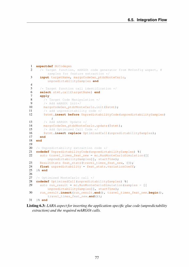
6.5. Integration Flow
1 aspectdef McCodegen2 /* Target function, mARGOt code generator from McConfig aspect, #
samples for feature extraction */3 input targetName, margoCodeGen_ptdrMonteCarlo,
unpredictabilitySamples end45 /* Target function call identification */6 select stmt.call{targetName} end7 apply8 /* Target Code Manipulation */9 /* Add mARGOt Init*/
10 margoCodeGen_ptdrMonteCarlo.init($stmt);11 /* add unpredictability code */12 $stmt.insert before UnpredictabilityCode(unpredictabilitySamples)
;13 /* Add mARGOt Update */14 margoCodeGen_ptdrMonteCarlo.update($stmt);15 /* Add Optimized Call Code */16 $stmt.insert replace OptimizedCall(unpredictabilitySamples);17 end18 end1920 /* Unpredictability extraction code */21 codedef UnpredictabilityCode(unpredictabilitySamples) %{22 auto travel_times_feat_new = mc.RunMonteCarloSimulation([[
unpredictabilitySamples]], startTime);23 ResultStats feat_stats(travel_times_feat_new, {});24 float unpredictability = feat_stats.variationCoeff;25 }% end2627 /* Optimized MonteCarlo call */28 codedef OptimizedCall(unpredictabilitySamples) %{29 auto run_result = mc.RunMonteCarloSimulation(samples - [[
unpredictabilitySamples]], startTime);30 run_result.insert(run_result.end(), travel_times_feat_new.begin(),
travel_times_feat_new.end());31 }% end
Listing 6.3: LARA aspect for inserting the application-specific glue code (unpredictabilityextraction) and the required mARGOt calls.
77
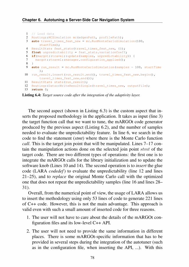
Chapter 6. Autotuning a Server-Side Car Navigation System
1 // Load data2 Routing::MCSimulation mc(edgesPath, profilePath);3 auto travel_times_feat_new = mc.RunMonteCarloSimulation(100,
startTime);4 ResultStats feat_stats(travel_times_feat_new, {});5 float unpredictability = feat_stats.variationCoeff;6 if(margot::travel::update(samples, unpredictability)) {7 margot::travel::manager.configuration_applied();8 }9 auto run_result = mc.RunMonteCarloSimulation(samples - 100, startTime
);10 run_result.insert(run_result.end(), travel_times_feat_new.begin(),
travel_times_feat_new.end());11 ResultStats stats(run_result);12 Routing::Data::WriteResultSingle(travel_times_new, outputFile);13 return 0;
Listing 6.4: Target source code after the integration of the adaptivity layer.
The second aspect (shown in Listing 6.3) is the custom aspect that in-serts the proposed methodology in the application. It takes as input (line 3)the target function call that we want to tune, the mARGOt code generatorproduced by the previous aspect (Listing 6.2), and the number of samplesneeded to evaluate the unpredictability feature. In line 6, we search in thecode to find the statement (stmt) where there is the Monte Carlo functioncall. This is the target join point that will be manipulated. Lines 7–17 con-tain the manipulation actions done on the selected join point stmt of thetarget code. There are two different types of operations: the first one is tointegrate the mARGOt calls for the library initialization and to update thesoftware knob (Lines 10 and 14). The second operation is to insert the gluecode (LARA codedef ) to evaluate the unpredictability (line 12 and lines21–25), and to replace the original Monte Carlo call with the optimizedone that does not repeat the unpredictability samples (line 16 and lines 28–31).
Overall, from the numerical point of view, the usage of LARA allows usto insert the methodology using only 53 lines of code to generate 221 linesof C++ code. However, this is not the main advantage. This approach isvalid even with such a small amount of inserted code for three reasons.
1. The user will not have to care about the details of the mARGOt con-figuration files and its low-level C++ API.
2. The user will not need to provide the same information in differentplaces. There is some mARGOt-specific information that has to beprovided in several steps during the integration of the autotuner (suchas in the configuration file, when inserting the API, ...). With this
78
6.6. Experimental Results
automated insertion, the information has to be provided only once,thus reducing the error probability.
3. This approach allows separation of concerns. All the extra-functionaloptimization, including the proposed approximation methodology, arekept separate from the original application. In this way, the developerof the original application does not need to be involved in the opti-mization process.
6.6 Experimental Results
In this section, we will show the results of the proposed methodology ap-plied to the PTDR algorithm. The platform that we used for the exper-iments consists of several nodes equipped with Intel Xeon E5-2630 V3CPUs (@2.8 GHz) with 128 GB of DDR4 memory (@1866 MHz) on adual-channel memory configuration. At first, we analyze the results of themodel training, needed to build the model that estimates the expected er-ror (see Section 6.6.1). Then, in Section 6.6.2 we validate the approach byverifying that it satisfies the constraint imposed on the error ε. We comparethe proposed approach to the original version, which decides the numberof samples a priori to satisfy the worst case, in Section 6.6.3. Finally, inSection 6.6.4, we evaluate the overhead introduced, and in Section 6.6.5we evaluate the optimization impact on the whole process, at system level.
6.6.1 Training the Model
As we already said, before using the proposed approach we need to trainthe error prediction model. So, the first phase is done off-line, and it con-sists in training the error model ( ˆerrorxi,y). This is done, as presented inSection 6.4.2, by using a different number of samples. To train the quantileregression model, we profiled data extracted by running random request tothe PTDR algorithm on a training set. The training set has been built us-ing 300 different paths across the Czech Republic, all characterized withtime-slots. In this way, we are able to consider different speed-profiles foreach segment of the paths. All the requests have been made for all the fourlevels of sampling used by the proposed methodology (i.e. 100, 300, 1000and 3000, as described in Section 6.4.2). The output of the model trainingis represented in Figure 6.6. The points in the three plots represent the out-put of the profiling runs, and are the same across the different images. Thelines are the quantile regression lines, which is the model that will be usedat runtime. The three sub-figures are different for the value of the quantile
79
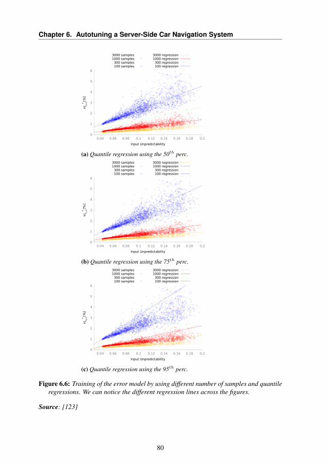
Chapter 6. Autotuning a Server-Side Car Navigation System
0
1
2
3
4
5
6
0.04 0.06 0.08 0.1 0.12 0.14 0.16 0.18 0.2
ν τ u
i,yx [%
]
Input Unpredictability
3000 samples1000 samples300 samples100 samples
3000 regression1000 regression300 regression100 regression
(a) Quantile regression using the 50th perc.
0
1
2
3
4
5
6
0.04 0.06 0.08 0.1 0.12 0.14 0.16 0.18 0.2
ν τ u
i,yx [%
]
Input Unpredictability
3000 samples1000 samples300 samples100 samples
3000 regression1000 regression300 regression100 regression
(b) Quantile regression using the 75th perc.
0
1
2
3
4
5
6
0.04 0.06 0.08 0.1 0.12 0.14 0.16 0.18 0.2
ν τ u
i,yx [%
]
Input Unpredictability
3000 samples1000 samples300 samples100 samples
3000 regression1000 regression300 regression100 regression
(c) Quantile regression using the 95th perc.
Figure 6.6: Training of the error model by using different number of samples and quantileregressions. We can notice the different regression lines across the figures.
Source: [123]
80
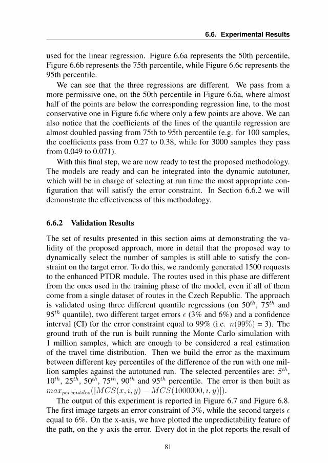
6.6. Experimental Results
used for the linear regression. Figure 6.6a represents the 50th percentile,Figure 6.6b represents the 75th percentile, while Figure 6.6c represents the95th percentile.
We can see that the three regressions are different. We pass from amore permissive one, on the 50th percentile in Figure 6.6a, where almosthalf of the points are below the corresponding regression line, to the mostconservative one in Figure 6.6c where only a few points are above. We canalso notice that the coefficients of the lines of the quantile regression arealmost doubled passing from 75th to 95th percentile (e.g. for 100 samples,the coefficients pass from 0.27 to 0.38, while for 3000 samples they passfrom 0.049 to 0.071).
With this final step, we are now ready to test the proposed methodology.The models are ready and can be integrated into the dynamic autotuner,which will be in charge of selecting at run time the most appropriate con-figuration that will satisfy the error constraint. In Section 6.6.2 we willdemonstrate the effectiveness of this methodology.
6.6.2 Validation Results
The set of results presented in this section aims at demonstrating the va-lidity of the proposed approach, more in detail that the proposed way todynamically select the number of samples is still able to satisfy the con-straint on the target error. To do this, we randomly generated 1500 requeststo the enhanced PTDR module. The routes used in this phase are differentfrom the ones used in the training phase of the model, even if all of themcome from a single dataset of routes in the Czech Republic. The approachis validated using three different quantile regressions (on 50th, 75th and95th quantile), two different target errors ε (3% and 6%) and a confidenceinterval (CI) for the error constraint equal to 99% (i.e. n(99%) = 3). Theground truth of the run is built running the Monte Carlo simulation with1 million samples, which are enough to be considered a real estimationof the travel time distribution. Then we build the error as the maximumbetween different key percentiles of the difference of the run with one mil-lion samples against the autotuned run. The selected percentiles are: 5th,10th, 25th, 50th, 75th, 90th and 95th percentile. The error is then built asmaxpercentiles(|MCS(x, i, y)−MCS(1000000, i, y)|).
The output of this experiment is reported in Figure 6.7 and Figure 6.8.The first image targets an error constraint of 3%, while the second targets εequal to 6%. On the x-axis, we have plotted the unpredictability feature ofthe path, on the y-axis the error. Every dot in the plot reports the result of
81
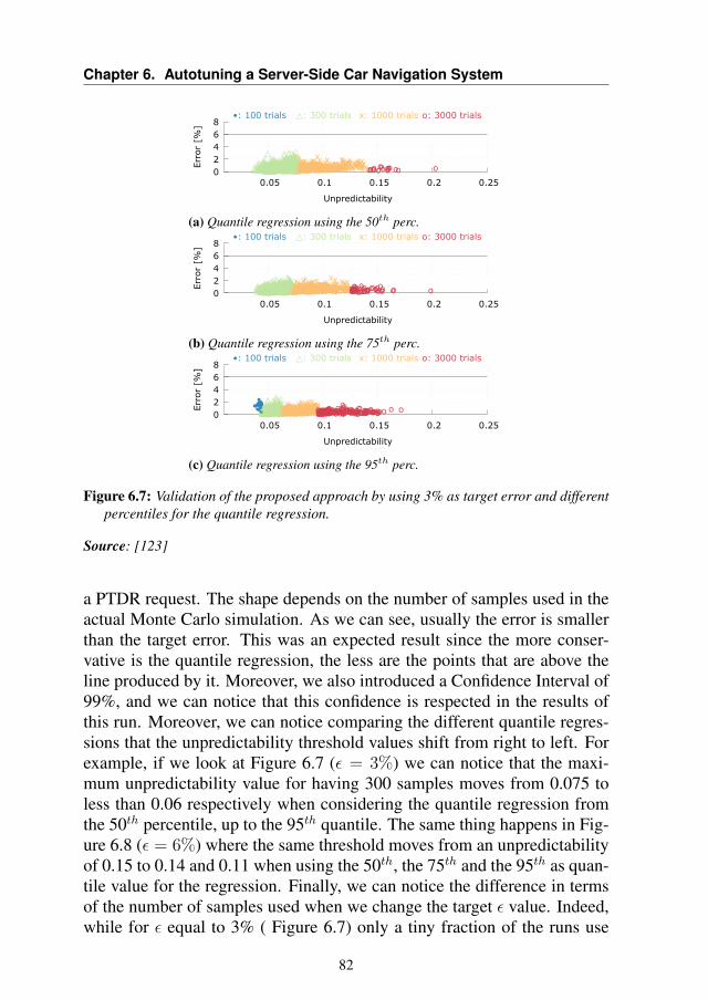
Chapter 6. Autotuning a Server-Side Car Navigation System
0 2 4 6 8
0.05 0.1 0.15 0.2 0.25
•: 100 trials △: 300 trials x: 1000 trials o: 3000 trials
Err
or
[%]
Unpredictability
△ xxx△ xx△△ xx△△ △ xx△ x△△△ xx xxx xx△ x△ xx△ x△ xx△△△△
x△ △ x△
x△ x△
x△ x x△
x△△△△ xx x△ x△△ △△ x△△ △△△ x xx△△ xxx△△
△ ox△ xxx△△△ x x△ x△ xx△ x xx
xx△△△ xx△△
x△ △ x△△ x△△ x△ x
△ x△ x x△ x x△ △△
x△△△ x△△△ △ x△△ x x△△△ △ x△△ x△△ x△ xxx△ x△△ x
△x△ xx
x△△△△△△
△ x△ △△ x x△ △ x△△ x△ △△ △ x△△
xx△△ △△△
△ △△△ xx△xxx△ △△
△x△ o△△
△xx△ x x
xx△△△ x△ △ x△△
xx△ △△ x△ x x x△
x△△△ x△
x△x
△ xx△△ △△△ x△ △ xx△△ x△ x△ △
△x△ △ x△△ △△
△△ xx△ △△△ △ x△△ xx△ x△ x△ xx△ x△ △ x△ △△ o△ x△ x xx△ x△△△ x△
x△△△ x△△ x△
△xx△ x
△ xx△ x△△ x△△ xx△△ x xxx
x△ x△
△△△△△ △ x△ △x△ xx△△ x x△ x△△△ x
△x x△ xx△ x△ x
△△ △△ x x xxx△ x△ x△△ △ x△ x△△ △ △ x xx△△△ △ x△ △ xx△ xxx△△ △ x△ △△ x△ x△ x xx△ x△ x△
x△ x△ x△ x△ xx x
x△ x△ x△△x
xx△ xx△ x△ x△△ x x△
x△ x△ △ x△ △△△ x△△△ x△ xx△ △△△△ △
x△ △ x△△△ △△x
△x△△△△△ △△△△△
△△ △ xx△ △△
xx△△ x△△x
△
△ x△x
x x△ x△△△
△ xx△ x△△ xx x△ xxx x△x△△ xx x△
△x
x△ x△△ xxx xx oxx△ △ x x△ xxx
x△△xx△△
△x△
△△△△ xx△△△△△
△△x
△ x△△ △ x△ x x△ xx o△△ x o△ x△△△△△ △ x△△ △△ △ x△△ x△
x ox△△△ x△
△△△△△ x△ △
xx△△△ xx xx△
△△ △△x△
xxx△△ x xxx△
xx△ xxxx o△ △x△ xx xx△
△△ △ x△△△ △△△△△△△ xxx△△ x△ x△△△ x△ xx△
△△ x△
x△△ x△ xx△ x△△ x△ xxx△
△ x x△ △
xx x△△ x△ xx△ x△△ xxx△ x△ x△ xx△ x△△△
xxx△ x x△
△△ x△ x△△ x△△ x x△ x△△ x△ x△△
xxx△ xxxxx
△△
△△ △△△
x△△
ox xx x△△ △
△△△△ xx x x
xxx△ △ x△ x△ △ x△ x x x△△ x△△ x△△△
△△△△ x△ x△ xx△
△ △ xx△ x x△△△
x x△△△△△ xx△△
x△ x△xx△ △△ △△ x△△ x△△ xx△ △x x
△x△ x x xx
△o△ xx△ x△ x
△ x△ △ x△△△△△△△△
△△△△ x x△△ x△ x△△ xx△ x△△△
x△△
xx ox△ xxxx△ x△△△
△ △ x△ △△ x xx x△ x△ xxxx△xx△ x
△△△ x△ ox△ △ xx△ x△x ox
△△
△△ x△
x△ x△x x△ △△ x
△ x△ x△ △△ xxxxxx xxx△ x x△ x△△ x△ x△
x△△x△ x△ x△△ △△△ △△△ △△ xxx△△ x o△△△△ xxx△ xxxx△ x△ x
△x xx△△△ x△ oxx△ △△ o△△△ x△△△△ xxx
△△ x xx△△△△△
△
△△ △ x x△ x△ x△ x△ x△△ x x△ x△ x
x△△ xx△ x x△△ x x△ xx xx xxx
△△ x△ xx△△△ △ x x△△△△ △ x△xxx△△△△ △△
x x△△△△ △△△ x x△△ x
△△△
△△△
xx x△
xx△
o△ x△ x△ x△△ x△ xx x
△x△ x△△
△x△ △△△ x△ xx△△△△x△ △△ x△
△△
x x△△ xx x△△ xx x△ xx△ △△ x△△ xx x xx△△ x△ x△ x x△△
△x
△ x△△△ △△△△ x△ △△△ x△
o△△△x△
△
△△ x xx△ △ x△ △△ x△△△ △ xx x△△△ x△ △△ △△ △ x△
△△ x△ △
△△△ △△ xx△△
xx x△x
△x△ △△△△ x
x△△ △
△△△△ xxxx△△△ △△ △△ x△ x
△ △
xx△ △ x△△ △△ x x△ xx
△△ x△
(a) Quantile regression using the 50th perc.
0 2 4 6 8
0.05 0.1 0.15 0.2 0.25
•: 100 trials △: 300 trials x: 1000 trials o: 3000 trials
Err
or
[%]
Unpredictability
△ xxx△ xx△ x xx
△xx ox△ x△△△ xxxxx ox△ o△ xx△ x△ xxx△x△ x△ x x△ x△ x△ x△
xx△
xx△△△ xxx△ x△△△△ x△△ xx
△ xxx△ xxx x△ x△ ox△ xx x△△ △ xx△ xx x△△ x ox x xx△△ xxx△ x△ △ x△ △ x△△ x△△
x xxx x△ x o△ x△ x△△△ x△△△△ x△△ x x△ x△△
xxx x△
△ x△ xx△△x△△ x△x△ xx
x△△ x△△△△ x
△ △x x x△ x x△△ x△△
△ △ xxx xxx△ x△ x△ x△
△ xxx x ox△ △△ x x△ o△△ x x△△ x xxxx△
△ x△x
x△ △ ox△ x△ x△ xxxxx△ xx x△ xxxx xx△△ △△ x x△△ x△△ △ x△ △△ △△
x△△ x△△△ x x△ xx△△△△ △ x△△ x x
△ x△ x△ x△△ x△ xx△ x△ oxx△ x ox△ x△△△ x△△
xx△ xx△ xxx xx△ xx xx△ x△ x x△△ x xx△ xxxx
△△ x△ x△ x△△ △ o△ x x△ xx△△ x xx x△ △△ x
△ x x△ xxx x△xx△ x△ x x xxx△ xx x
△△ x x△ △△△△ x x xx△ △△ △△△ △ xx△ xx△
△△△ x△△△ o△ x△ x
xxxx△ x△x△ x△ x△ xxx x x x△ x△ x△△ x xx△ x△△ x△ x△△ xx△ x△ x△
x x△ x△△ x△ △△ x△ xx△ x x
x△ x x△ △ x△△△ xx x△ x xx△△△ △ x△△
△△ △△ xx△△△ xxx△ x△△ o△△ x
x xxx△ o△△ x△ xx△x△△ xxx
△ x xx xxx△△ x x ox△ xx△ x△△ xxx xx oxx△ xx x△ xxx x△△ x
x xx△x△ x△xx x△△△ xx△x△ x△ x△
△△ xx x o△
xx ox△ x o△ △△△△△ △△ x△△△△ x△△△
xx x oox
△△ ox△△
△x△ x△△ xxxx△ xxx△△x△ △△ x△ x ox△△ x xxxx xxx oxx x o△ △ o
△ oxxx△△△△ x△△△ x△△△△△△ xx△△
△ x△ x△△△ x△
x xx△△ xxx△△ x△ xx△
x△ x x△ xx x△x x x△△
xx xx△ x△ xx△ x△△ xxx△ x△x△ x
x△ x△△ △ xx x△ x x△ x△ x△ x△△ x△△ xxxx△ △ x△ x△△ xxx△ oxx o o△ xx△△△ △
△x△ ox ox x△△ △ x△
△ △ xx x xxxxx xx
△ x△△ x△ x x x△
△ x△△ x△△△ x△△ △
x△ x△ xx△△ △ xx△ xxx△ x x
x△△△△△ xx△ △ xxxx x△△△△ xx
x△△ x△ x xx△ xx
xx x△ x xxxx o△ x△△
x△ xx o△ △ x△△ x△ △△△△△ xx△ x xxx xx
△△△ xx△ x△△ x xxx ox ox△ xxxx△ x△△△△ △ x△ x
△ xxx x△
x△ xx xxx△
x△xx△ x x△ ox
△△ x△△ x△ x ox△△△△ xxx△ xx x o△ △△ x
△ x△ xxx△ xx xx xx oxx△
x x△ △ xx x△ xx
xx△ x△x△ x△△ x△△ △△△△△ xx x△ xx o△
△ xx xxx△ xx xx△ x△ x△ x xx△△ xx△ oxx△ xx
o△△
△ xx
x△△ xx x△△ x xx
△ x△ △△ x△△ △ x o△o△ xx x△ x△△ x x△ x△ △ xx△ x x△ △ o
△△ xx△ x△
xx xxx△△ x△xxxx△ x xx△△△△ △ xxx
△ x△△△△ xx xxx△ △△ △△△ x x△△ x
x△△△△△ xx x△ xx△ ox△△ x△ x△△ x△ xx x△ x△ xx△ x△△△ xx x△ xx△△△△ x△ x△ xx△△ xx△△ xx x△△ x x x△ x x△
x△△△△ xxx xx△△ xx x△ △ x△
△ △ xxx
△△△ △△△△ x△ △△△ ox o△
x△ x△△
△△x
xx△△ x△ x△ oxx△ xxx x△△△ x△ x
△x△△ x△ x△x
△ △△ △△ △△ xx△△ xx xx xx△△ △△△△ x x△△ △ xx△ △ xxx x
x△△△△ △△ x△ x△△ x x△△
x△△ △ x x x△ xxx△ x△
(b) Quantile regression using the 75th perc.
0 2 4 6 8
0.05 0.1 0.15 0.2 0.25
•: 100 trials △: 300 trials x: 1000 trials o: 3000 trials
Err
or
[%]
Unpredictability
△ x x o△ xx△ xx xxx x ox△ xxx△ ox oxx ox• o△ ox△ x△ x oxxx△
xx△ x△ ox x△ xx oox xx△△△ xxx△ o△
△xx o
△△ xx△ x x x△x x xxx xx oxx xoxx△△ xx△ x
x x x△ x ox oxx△△ x xxx o
•x x△ △ xx x o△ xx xxx x△ x o△ xx xx△ x o△△△ xx△
•x ox xxx x△x o△ x x△ x xx x xx△ xx ox ox ox x xxx x△ o△ xx xx
xx x△• o△ x△ x oxx xxx△ xx x△ x△△ xxx o ox△△△ x o△ o△△ x ox△ x o ox
x△•
x△ x x△ △ ooxx•
o△ xxxxx△ xx xx ox xx ox△
xx xx o△x
xxx△ xx x△ x xx△△ x
△△ △ xx△ oo△△△•
x x△△ oxx o△
o△
xxx o△ x x△ x△ ox x
x x oo△ o△△
x x△ x xxx ox△ ox△ xxx xx ox△ x△ x x•△ x xx△ o oxxx△ x
•x△ xx△ x o△ xxx
xxxx x ox x△△
△x△ oo△ ox
xo
x xx
△ x△ xx oxx△ x x ox△ x x△ x△△△
xx ox△△△ x x△ x ox
x oxx△ x△x
△△△ ox ox x oxx xx
oxxx x△ oxxxxx
o ox x△ x△△x
x x△ xx△ o
△o△△ oox o△ x△ x x△ xx△ x△ x• xx ox△ xxxx
xx△ x o△△△ xx xx xxx△△△ x x△ x△△xx oxxxx ox
x△ox△ ox• ox o
x o△ ox△ x△ xxx oxxx x o△ o ox oxxx△ ox o△△ o o△ o△△ xxx ox oxx
△xx
xx
xxx xxx xxx xx x
△xxxx oxx
△ xxx x△ o△ ox△△ xxx ox xx oxx o oxxx
△△△ xx ox△△
△ x x△△ ox x ooxx△ ox△• xx• x△ x oxx x• xxx xxx△△
xx
x x ox△•
x ox xxxxx oxxx o• △ ox ox x
x△△ x x xx△△ x△ x△△△△ x△
xxx ox xx x△ x△ xxxxx x xxx△ ox xx△ ox x ox xx oxx x o
△x x x ox• xx ox△ o△ x xxx△ oxx△ oox xx△ △ oxx△
xo△ xx xx x△△ ox△ xxx x△△ o△ x• △ oxx△ oxx o oxx
x• x△ x xx△ ox ox
x△△ xxxxx xx x ox oxx xxxx△△ x△ xx ox• xx△ x△△△ x△△ △ x△ o△ xx△△ x ox△ x xx△ x x oxx
△△△ xx△ x ox xx xx△ x△ xx x△△ xx x oo△ xx ox o△ xx ox△ o△ o△△ o△ xx o△ x
x△△△
△△△△ △△ xx△
x oxx xxx
x△ ox△ xx△ x oxx ox oox oxx x
•xx xx△ x oxx
△xxx ox x
△ xx ooxx x△ x o△ x ox oxx xxx△ x△ x ox•△ x xxxx△ x△ o
o△ x△ xx xx x△
xxx
oxxx
x oxxx xxxxxxo△ ox o
△△ o△ xx x△△ x△△ x△△ xx oxx
xx x oxx xx xxxx xxx xx ox x△
x oo△△ x ox ooxx xx ox△△ xxx△
△ x xxx
x o oxx x△ x• x△△△ o o△ ox ox ox o△•
x o△ xxxxxxx x△ x oxx xx△ xx ox xxxxx xx xox x△ xx xx△△△ x xxxxxx△△△ xx xox△ x
•x△△ x ox△ xx△△ x△ △ oxxx ox
△ox
xx x△ x△
△ xx ox xx xx xx•
xx△
x xxx
△ x xxxx• x△ xx ox△ △ oo△△ xx x△△ ooo△ x x△ xx xx△ ox x oxx△ ox x△ x ox△ x ox o△x△ x xx△ x△ x
△• ox o△ x△ xxxxx x oo△△
x△ x△ oxx△ x xx o△△△ oxxxx△ x xx xx x△△△ x△
x△ o oxx oo ox xxx• △xxx x
o△△ xxx△ x xxx xxx△ x△ x△ xx x△ xx o△ xx△△ xx oo△ oxx△ xx
(c) Quantile regression using the 95th perc.
Figure 6.7: Validation of the proposed approach by using 3% as target error and differentpercentiles for the quantile regression.
Source: [123]
a PTDR request. The shape depends on the number of samples used in theactual Monte Carlo simulation. As we can see, usually the error is smallerthan the target error. This was an expected result since the more conser-vative is the quantile regression, the less are the points that are above theline produced by it. Moreover, we also introduced a Confidence Interval of99%, and we can notice that this confidence is respected in the results ofthis run. Moreover, we can notice comparing the different quantile regres-sions that the unpredictability threshold values shift from right to left. Forexample, if we look at Figure 6.7 (ε = 3%) we can notice that the maxi-mum unpredictability value for having 300 samples moves from 0.075 toless than 0.06 respectively when considering the quantile regression fromthe 50th percentile, up to the 95th quantile. The same thing happens in Fig-ure 6.8 (ε = 6%) where the same threshold moves from an unpredictabilityof 0.15 to 0.14 and 0.11 when using the 50th, the 75th and the 95th as quan-tile value for the regression. Finally, we can notice the difference in termsof the number of samples used when we change the target ε value. Indeed,while for ε equal to 3% ( Figure 6.7) only a tiny fraction of the runs use
82
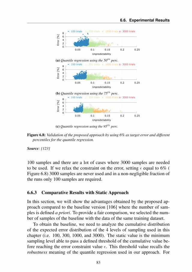
6.6. Experimental Results
0 2 4 6 8
0.05 0.1 0.15 0.2 0.25
•: 100 trials △: 300 trials x: 1000 trials o: 3000 trials
Err
or
[%]
Unpredictability
• • △△• •
••• •••
• • x•
••••• △• • △• △•
• △•△
△• •• △△•
•
•
••••
△• △• •
• ••△△•
△•
••• ••
•
• ••• •• △•• ••• △△△•
••△•
• ••△
••△
△△
•••
•
△•••
•
••
△△• △△•
•••△
•••
• • △• • •• • △• ••
△••
△•• △
••• △•••
△••• ••
•• •
△
•••• ••
• △• • △• •
•
••
△•• •
•
△••
•
△
• •• •••• △
• •••
•
•
•
△•• △•
•• • △•• △△••
•
•
••
•••••
•△ △
•• •• •△
• x•
• • △••• △
△△••• •
• •△
• •△△••
• △• ••△
••••
• △• △• △•
△•••
•
••△• • △•••
•• •• • • •
• •
△
••
•••• △••
••• • △•• △△
•△
••• •
•• △• ••• •
• x•△•
△ △△• △•• • △•
• •••
△
•• △•• • ••
△• △
△• ••• △•• •
••• △ △• △•• ••
••
•••
•
△•
•
•
• △△•• •
△•△••••• •
△• △△•
△• △•
• •••• △
•△• •• △••
••
•••
• • • △ △•••• • •• • △
•
•△
•••
• • △••• x• △
•
△△△
••• •
•••△•△• △
••
△ △△• △• •••△
• △• △•• •
• △•• △△• △
•••
•
△••
••••
•• △• △△• •
••
•• •• ••
••• •• •••• •
••• • •• •••
•• △
•••
•△••• △
•• △•• △
•
△• △• △• ••
• • △•
△• • •△ △• △ △• △△
••
• ••
△•• △•• △•
• △•
△
△•
△△••• •
•• •
△••
•• ••
••• △•••• •
•••• •
•• •
•
△• △••• ••• △•
•• △•• △
x•••
••• ••△•• •
• ••
•• △• • x
△•
•• △
••• ••• •
•• △△
••
•△
•••• ••••
•
•△
△••• •
•
•••••
•
△△△△△
••
△• △• •△•• • • •
••• △•
•
•• ••••••• △• △
••• △
••△•
•••
•••• △•••
••••
•
• △
•△
•• • △• • •
•△••
•• • △•
△••
•••
•△•
•• △
△• △•• • △
•△
• △△•
••
•
• ••• △••
△•
• ••• △•
••• △••
•△
△• △△
•••
••
••
△•• △
•△
• △•• •
••• • •
•△△
•△
•• △•• ••• •• •△
△•
•••
• △•••
••• • △
•
△•
△
•
••• △
••
••
••
•
△△
•••• • △••
•
△••
•
•
•••• ••
•
•
•••
• △△• ••
△• △•△ △△
•• △• △•• △• •• △• • △•••
•••••• • •
• •△
•
•
••
•••△
•• •••
• △•• △
•x△• △•• △•
••
•••
• △• •• ••• △•
••△△
△△
△• •
•
••• • △• △•• •
△•• •
••
△•
•••
•△• •
• ••
△
△••
• •• •• •• ••
△ △
• △•△ △•
•
• △△•••
•△
• △•△
•• △
• ••
••• ••• ••• •• △
•
△••• △
•• •• •
•
••
△•
△•
•△• △• △
△△•• • •• △△
•• ••x
•••
• △•••
• △•
••• △•• •
••
• ••• • • △•
△• △•
△••
••
•
△• △•
△
•
•• •△
•• △
••
△•
••• △•
•△ △••△
• •△
•••
• ••••••
• △••••
•••• •• • △•••• ••• • △
••
△•• • •
•• △•
••
△••
△• •• •• △•
•△
• △••
• ••
••• •
•• • ••△
• •△
•••• •
• •• △•• •
△△•
• •• △
•• △•
△
•• •
••••••
△••
△•
•••
•
•• • △•• •
△•
△••••
•
••
••
••• △• x• •• △••
•••
△△• •△• ••
△
•
•••
•
•
△•
•• △•••
••
••
•
•• •••
• •• ••△
△
•
•△△△•
•••• ••••
• △••
••
•••
•••△•••
••
•• ••
•
•
••△
•
• ••• •• △△• △••
• ••
(a) Quantile regression using the 50th perc.
0 2 4 6 8
0.05 0.1 0.15 0.2 0.25
•: 100 trials △: 300 trials x: 1000 trials o: 3000 trials
Err
or
[%]
Unpredictability
•
△△ △• △••
•△ △•• △ x△• △•••△
•△
•
△ △•• x
• △
•
• •• △△••••
•• • △• △• △•
•• △△• △••
•• △
•
•
• △••
•
•△•• △
•• △△△•• △△△•△
• x△• △△△•
••△
••
•
• •
••
△ △• △△••
•
•△
•
• △• •
△
•• △•
• △•••
△△
•△•
•x•
•• △••• △••••
••
•
•
△•• •
•△•• △•
••• ••△
•△•• △•△• △•
•••••
•••
△•
•• △△• • △•• △••
• •
△•
• △△•• •
••• ••• △
••
△△△• •• • △
• x•• △ △•• △ △ △△•••••
• △• • △△••• △••△ △
•
△• △
• △• △• △••
△•
• •• • △• • △
△•
•
△• △• •• △
• ••
•• ••
••x△
••••
•△• •△△•
△• △•
•••△
• ••• •• x•△• • △△• △•••
△• ••
•• △
•• △•• △△• △• △
△•△
• • △••• △••
△ △△•
•• •• •• •••• △•• △•
△△
•• •
△
•△• •• •
•△△• △△
• △• •••
••
• △ △△△• △•
△•• ••• •••• △△
△△• •• • •• • △•• △△
••• • △•••
x• △• △
x△••• △
•△
• △• △•
△• • △△△•
△• △• ••••
• △•• △•
△•• △△• △•
△•
△△•
••• •• •• △• △△• △••• • △• • △••• ••△• △••
••• • •• •••
•
•
△
△•
••
△△•• △
••x•• △
•△△△• x
••
•• △ △• △•
••△ △
•
△
△•
△•••
•△△ △•• △ △
•△
••
△△△△△ x△△• • △
△•
△△△△•• △△△•
••
••
••
• △△•• △•••• △
•△••• △• △ △• △
△ x
•• △ x
• ••
••• •• △•• •• •
••• △
• △x△••• △
•
•• •••
•• •△△
••
•
•
△△△•••
•• △• x△••• △△
•△△•△• △△
△ △ x• • △• x△ △△••• • △
••• ••
••• •• •••
••
△•
△• •• △• △••• •
△
•
△•
•
△• △•
•△
•• △• △• △•••
△• • •• △
•
• △••
△•△•• △
•••
△•••
△△• △•• •△
△△• • △• ••••
••• △•• △△
• △• •△
• ••
• △△•• △△• △△•• △• •
••△•• x△ x• △•
• • △•
••
• △ △△
• △•• △△
•△••△
• △ △ △•• ••
• △•••
•
•• • △• △• •△••
• △•• △
△••
•
△△
••••• △△••
△•
△• △•
••• △
• △•• •••
△△• •
•△• △• △
△△•• △• △•
• △•
•• x• •
△
•• •
• ••• • •• △• • △•• △
• •••△
△• •••
•△△• △△ x△• △△ △
△• △
•••
••
△••• • △△ △• △•
△△△△△
•
△•
△△•• △•
x△• •
△••
••
•x••• ••
△• △•
•• △x
••• •• △
•△• •
• △ △△ △△△
△△ △• △△•
••• △
•△• △• •△
• ••
•
•• ••••••
•• △
△△
•• △
△
•
••••△△• △•• △• △• △• △
•
△•
• △△•
x△
△• △
•x••• ••••• △•△•• △
△△
••
• •• △•• • △ △• △• △• △•
△•• △△
•△
•△△•
•△ △
• △ x•• △△• △•
△•△△
△•• △• △ △•
△• •
•
△•
••• ••••••
•• •• •• △
△•
• •••••
•△
•
• △•• ••
•• △•△• △•• △
••• △• △•
• △
• △△••△
•
•△•
•
•••
•△ △• • △••
•• •• •• △••
•△△
••
••
△•• △△ △• •△•
•••••
△• △△
•
•• △•
△••
△••
•△△△•
•• •
•••
•• ••• △△ x
• △• △•
• ••
△ △△• •△• •• x
••• •△△ △•
•• △• •• ••• •• •• △• •••••• △△•• △
△△• •
•△•
•••
• • △••
•
• •••
••△△
••• •• ••• •
△••△ △
• •△••
•
△△ △•△
••• ••
(b) Quantile regression using the 75th perc.
0 2 4 6 8
0.05 0.1 0.15 0.2 0.25
•: 100 trials △: 300 trials x: 1000 trials o: 3000 trials
Err
or
[%]
Unpredictability
• △△△•△△• △△△•△
△ x△• △••• △△ △△△ x△• x
•△
△• △• △△△•
△• △
••△
•x• △• △△ x△△ △••••
△△
•
• △•• △
△ △•• △△• △△
△• • △△△• △• x△• △△ △•••△△• △• △△• △
x△ △ △△•• △△•• △• • △•• △• △△
△△△ △△△ △•
△ x••
•
△△••
△••• △△••△ x
△△••
△△△
x• △•
• △△△△ △△• △• △• △△
x•• △△• △•
x•
•
△△ △• △ △•• △
••• △
△•
△ △△△• △•••••• △△• x x△• ••
△ △• x
•
• △△•
• △ xx△△••
△• • △• •
xx△△• △• △△ x△ △
• △△△• △
△△• △
△△• △
• △ x•
△ △△• △ △• △
••△ △•
• △•• • △△• x△•••
•• △•• △△△
x• △•△
•△ x• △
△••
•x△ △
•
△ x
△
• △△• △△• △△• △△
△
•△△
•△
△• △△ x△• △•
△△•
•
△
△△• △ x△ △△
•
••
△•△•
•△ x
• △△• △△△
•△ x
△ △• •• △•
△ x• △△△x• △△• △
• △ △x△△•
△△△•• △ △• △
•• • △△ x△• △• • △• •
x△• △△△•• △ △•••
x• x• △
x△△△• △
•△•
△•
△•
△• △△
xx
△
△• △• • △△△• △△• △
•x••
△△• △
• △• △△• △
•• △•△• △• △△• △△••• △
•
•△• △•
•
• △•△
△△•
••
• △• ••
••△
x△
••• △△△• x•• x
•• △△
x△ △
• x••△• △△
△ △•△ △△
△• △ x△ x△
△•
•△ △ x
••△ x• △•
•△△△
△△ x△△• △ △ △
△ △△△ △△• △△△△•△
• △ △•△ △△•△ △△• △• △
△ △••• △△
△
x△ △△ x△• x x△△△•••
••
△••
•
• △△•• △△ △ xx△•
• x△•• • △• △•• △△•
△• △△△△△△
•••△
• △x△•• △ △△
△△△ △
•x△ △
△x•• x
• x•
△△• •• △△•••
△• ••• •• △△•••
x• △△△• △• △ △△△△
△△△•• x△ x△• x• • △
△△
△△△•
•x• • △
△x△• △
•△△
•△
•△ △△ △
•
x•
△• x△• △
△•• x
△x
• △ △• △• △• △•• △△• △△△ △•
•x• △
•
• △△△• x△
△ x x• △△••
• • x•
• x△ x△△•
•△△••• △△ △ x△ x△
△ △△• △• • △• △△ x
△• △•
• △••••
•••
△• △• △△••
•
△△• △ △△•
•
△ x••••
• △△•△△△ △• △•
••• △△
x
••
△
△△
x△• △△ x△ x•
△x△
△•x
• △••
x• △
△ x• △△•
••
•••
••• △△•
△ △△
• △•
•
△• x△• △
••
•△△• x
△ xx△ x△△△• △•△•
•• △
•△• △
△△ x• △•△△ △△
△△ △• △△•
•
x•
x△•
△ △△
• △•
△ x△•• △ △△△ △
• •• △ x••• △△ △• △• △△
x△△△ △△x
△△
△ △△• △△△
x•△
△ △△•
△•
△•△••
••• △
•
••• △△ △
••△ x• △ △
• △△△△ △△△△• △• △• △
△
△•• △ △•
xx△△
••
x△•• △△△
••
•
△△△• △ x△•△• •• △•
• • △x
•x△ △• △
△ △•• △x• △
•
△
△△• △△• △
x△•△△• △△ x△△
△
△•• △• △△••
•• △
△△•• • △△△ △△△•••
• △• △
△△•
•• △••
△ △•• △△
• • •••x△
△• x••
x△△• △• △••
x•
x△△
•△• △△• △△• △ △△ △
• △△•••
• △••• △
••
• △△• • △△ △•• △△ x• △△
• △△
△△
•
x△
•
△△•• △△△•
△ x•• • x△△•
•• • △△•
△• △•• x△ x
•
△• △△△△
• △ △ x•• △• △• x△△•
△△△
x••• x
•△••
•• △• △• △• •• ••△• △ x△
•
xx x△ x△△• •••• △ x•
• ••△• • △△△ △△
•• ••
•
• △• △• • △△
••△△• △△ △ x• x△△
•△
•
(c) Quantile regression using the 95th perc.
Figure 6.8: Validation of the proposed approach by using 6% as target error and differentpercentiles for the quantile regression.
Source: [123]
100 samples and there are a lot of cases where 3000 samples are neededto be used. If we relax the constraint on the error, setting ε equal to 6% (Figure 6.8) 3000 samples are never used and in a non-negligible fraction ofthe runs only 100 samples are required.
6.6.3 Comparative Results with Static Approach
In this section, we will show the advantages obtained by the proposed ap-proach compared to the baseline version [106] where the number of sam-ples is defined a priori. To provide a fair comparison, we selected the num-ber of samples of the baseline with the data of the same training dataset.
To obtain the baseline, we need to analyze the cumulative distributionof the expected error distribution of the 4 levels of sampling used in thischapter (i.e. 100, 300, 1000, and 3000). The static value is the minimumsampling level able to pass a defined threshold of the cumulative value be-fore reaching the error constraint value ε. This threshold value recalls therobustness meaning of the quantile regression used in our approach. For
83
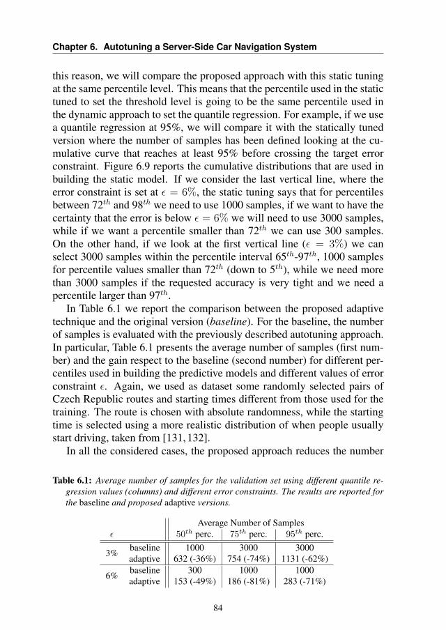
Chapter 6. Autotuning a Server-Side Car Navigation System
this reason, we will compare the proposed approach with this static tuningat the same percentile level. This means that the percentile used in the statictuned to set the threshold level is going to be the same percentile used inthe dynamic approach to set the quantile regression. For example, if we usea quantile regression at 95%, we will compare it with the statically tunedversion where the number of samples has been defined looking at the cu-mulative curve that reaches at least 95% before crossing the target errorconstraint. Figure 6.9 reports the cumulative distributions that are used inbuilding the static model. If we consider the last vertical line, where theerror constraint is set at ε = 6%, the static tuning says that for percentilesbetween 72th and 98th we need to use 1000 samples, if we want to have thecertainty that the error is below ε = 6% we will need to use 3000 samples,while if we want a percentile smaller than 72th we can use 300 samples.On the other hand, if we look at the first vertical line (ε = 3%) we canselect 3000 samples within the percentile interval 65th-97th, 1000 samplesfor percentile values smaller than 72th (down to 5th), while we need morethan 3000 samples if the requested accuracy is very tight and we need apercentile larger than 97th.
In Table 6.1 we report the comparison between the proposed adaptivetechnique and the original version (baseline). For the baseline, the numberof samples is evaluated with the previously described autotuning approach.In particular, Table 6.1 presents the average number of samples (first num-ber) and the gain respect to the baseline (second number) for different per-centiles used in building the predictive models and different values of errorconstraint ε. Again, we used as dataset some randomly selected pairs ofCzech Republic routes and starting times different from those used for thetraining. The route is chosen with absolute randomness, while the startingtime is selected using a more realistic distribution of when people usuallystart driving, taken from [131, 132].
In all the considered cases, the proposed approach reduces the number
Table 6.1: Average number of samples for the validation set using different quantile re-gression values (columns) and different error constraints. The results are reported forthe baseline and proposed adaptive versions.
Average Number of Samplesε 50th perc. 75th perc. 95th perc.
3% baseline 1000 3000 3000adaptive 632 (-36%) 754 (-74%) 1131 (-62%)
6% baseline 300 1000 1000adaptive 153 (-49%) 186 (-81%) 283 (-71%)
84
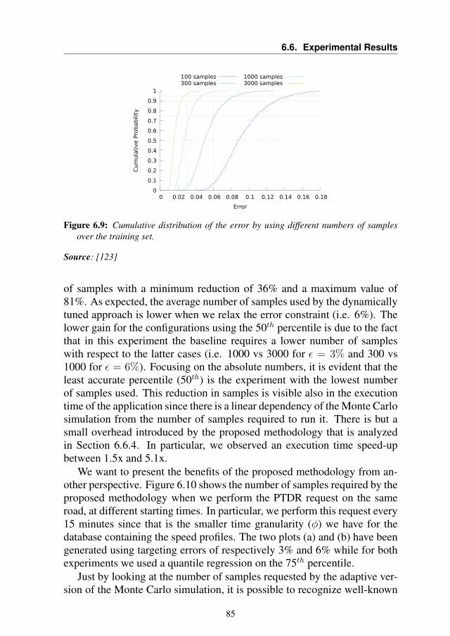
6.6. Experimental Results
0
0.1
0.2
0.3
0.4
0.5
0.6
0.7
0.8
0.9
1
0 0.02 0.04 0.06 0.08 0.1 0.12 0.14 0.16 0.18
Cum
ula
tive P
rob
ab
ility
Error
100 samples300 samples
1000 samples3000 samples
Figure 6.9: Cumulative distribution of the error by using different numbers of samplesover the training set.
Source: [123]
of samples with a minimum reduction of 36% and a maximum value of81%. As expected, the average number of samples used by the dynamicallytuned approach is lower when we relax the error constraint (i.e. 6%). Thelower gain for the configurations using the 50th percentile is due to the factthat in this experiment the baseline requires a lower number of sampleswith respect to the latter cases (i.e. 1000 vs 3000 for ε = 3% and 300 vs1000 for ε = 6%). Focusing on the absolute numbers, it is evident that theleast accurate percentile (50th) is the experiment with the lowest numberof samples used. This reduction in samples is visible also in the executiontime of the application since there is a linear dependency of the Monte Carlosimulation from the number of samples required to run it. There is but asmall overhead introduced by the proposed methodology that is analyzedin Section 6.6.4. In particular, we observed an execution time speed-upbetween 1.5x and 5.1x.
We want to present the benefits of the proposed methodology from an-other perspective. Figure 6.10 shows the number of samples required by theproposed methodology when we perform the PTDR request on the sameroad, at different starting times. In particular, we perform this request every15 minutes since that is the smaller time granularity (φ) we have for thedatabase containing the speed profiles. The two plots (a) and (b) have beengenerated using targeting errors of respectively 3% and 6% while for bothexperiments we used a quantile regression on the 75th percentile.
Just by looking at the number of samples requested by the adaptive ver-sion of the Monte Carlo simulation, it is possible to recognize well-known
85
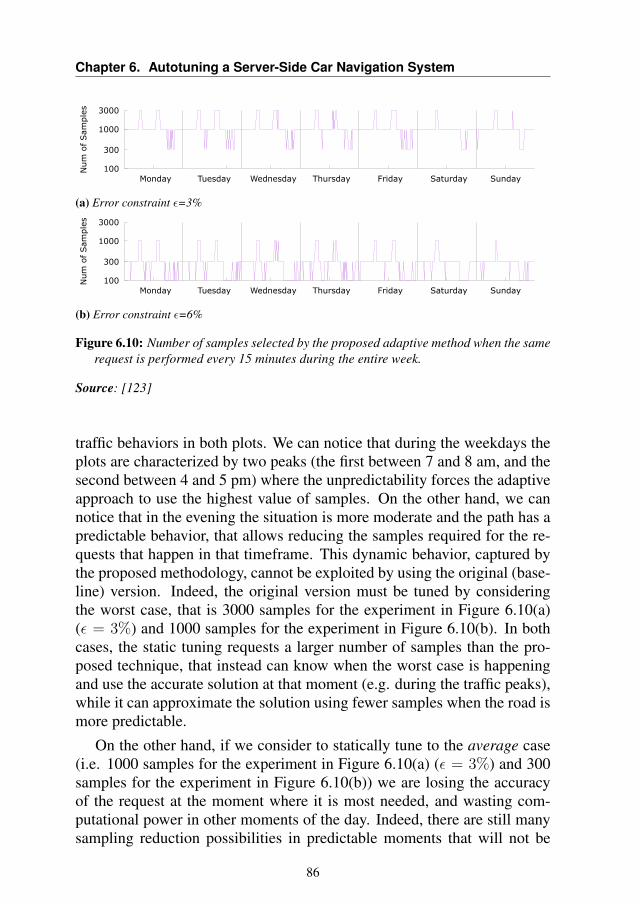
Chapter 6. Autotuning a Server-Side Car Navigation System
100
300
1000
3000
Monday Tuesday Wednesday Thursday Friday Saturday Sunday
Num
of
Sam
ple
s
(a) Error constraint ε=3%
100
300
1000
3000
Monday Tuesday Wednesday Thursday Friday Saturday Sunday
Num
of
Sam
ple
s
(b) Error constraint ε=6%
Figure 6.10: Number of samples selected by the proposed adaptive method when the samerequest is performed every 15 minutes during the entire week.
Source: [123]
traffic behaviors in both plots. We can notice that during the weekdays theplots are characterized by two peaks (the first between 7 and 8 am, and thesecond between 4 and 5 pm) where the unpredictability forces the adaptiveapproach to use the highest value of samples. On the other hand, we cannotice that in the evening the situation is more moderate and the path has apredictable behavior, that allows reducing the samples required for the re-quests that happen in that timeframe. This dynamic behavior, captured bythe proposed methodology, cannot be exploited by using the original (base-line) version. Indeed, the original version must be tuned by consideringthe worst case, that is 3000 samples for the experiment in Figure 6.10(a)(ε = 3%) and 1000 samples for the experiment in Figure 6.10(b). In bothcases, the static tuning requests a larger number of samples than the pro-posed technique, that instead can know when the worst case is happeningand use the accurate solution at that moment (e.g. during the traffic peaks),while it can approximate the solution using fewer samples when the road ismore predictable.
On the other hand, if we consider to statically tune to the average case(i.e. 1000 samples for the experiment in Figure 6.10(a) (ε = 3%) and 300samples for the experiment in Figure 6.10(b)) we are losing the accuracyof the request at the moment where it is most needed, and wasting com-putational power in other moments of the day. Indeed, there are still manysampling reduction possibilities in predictable moments that will not be
86
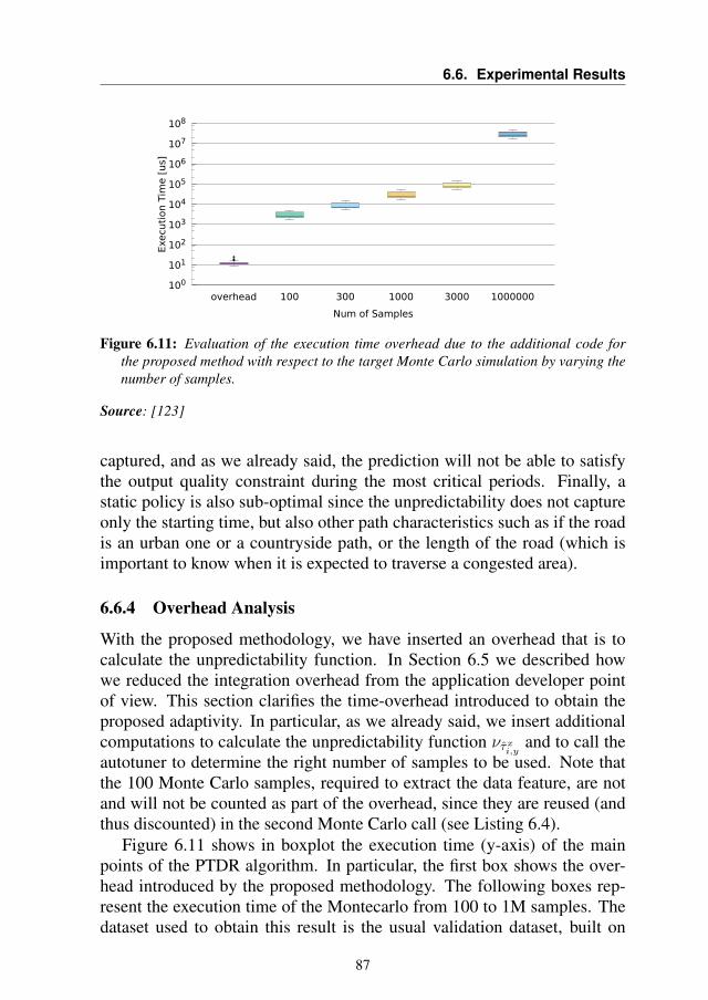
6.6. Experimental Results
100
101
102
103
104
105
106
107
108
overhead 100 300 1000 3000 1000000
Exe
cuti
on T
ime [
us]
Num of Samples
Figure 6.11: Evaluation of the execution time overhead due to the additional code forthe proposed method with respect to the target Monte Carlo simulation by varying thenumber of samples.
Source: [123]
captured, and as we already said, the prediction will not be able to satisfythe output quality constraint during the most critical periods. Finally, astatic policy is also sub-optimal since the unpredictability does not captureonly the starting time, but also other path characteristics such as if the roadis an urban one or a countryside path, or the length of the road (which isimportant to know when it is expected to traverse a congested area).
6.6.4 Overhead Analysis
With the proposed methodology, we have inserted an overhead that is tocalculate the unpredictability function. In Section 6.5 we described howwe reduced the integration overhead from the application developer pointof view. This section clarifies the time-overhead introduced to obtain theproposed adaptivity. In particular, as we already said, we insert additionalcomputations to calculate the unpredictability function ντxi,y and to call theautotuner to determine the right number of samples to be used. Note thatthe 100 Monte Carlo samples, required to extract the data feature, are notand will not be counted as part of the overhead, since they are reused (andthus discounted) in the second Monte Carlo call (see Listing 6.4).
Figure 6.11 shows in boxplot the execution time (y-axis) of the mainpoints of the PTDR algorithm. In particular, the first box shows the over-head introduced by the proposed methodology. The following boxes rep-resent the execution time of the Montecarlo from 100 to 1M samples. Thedataset used to obtain this result is the usual validation dataset, built on
87
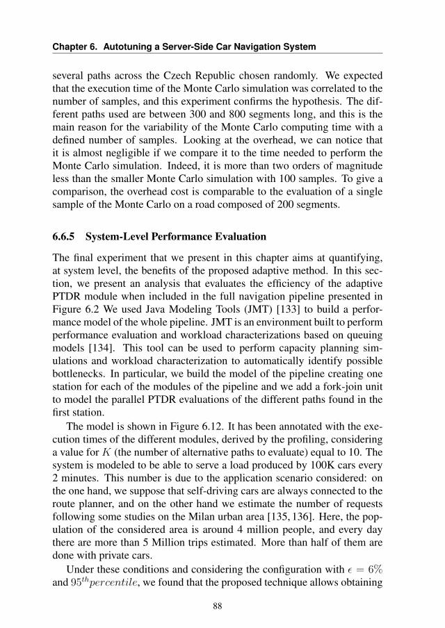
Chapter 6. Autotuning a Server-Side Car Navigation System
several paths across the Czech Republic chosen randomly. We expectedthat the execution time of the Monte Carlo simulation was correlated to thenumber of samples, and this experiment confirms the hypothesis. The dif-ferent paths used are between 300 and 800 segments long, and this is themain reason for the variability of the Monte Carlo computing time with adefined number of samples. Looking at the overhead, we can notice thatit is almost negligible if we compare it to the time needed to perform theMonte Carlo simulation. Indeed, it is more than two orders of magnitudeless than the smaller Monte Carlo simulation with 100 samples. To give acomparison, the overhead cost is comparable to the evaluation of a singlesample of the Monte Carlo on a road composed of 200 segments.
6.6.5 System-Level Performance Evaluation
The final experiment that we present in this chapter aims at quantifying,at system level, the benefits of the proposed adaptive method. In this sec-tion, we present an analysis that evaluates the efficiency of the adaptivePTDR module when included in the full navigation pipeline presented inFigure 6.2 We used Java Modeling Tools (JMT) [133] to build a perfor-mance model of the whole pipeline. JMT is an environment built to performperformance evaluation and workload characterizations based on queuingmodels [134]. This tool can be used to perform capacity planning sim-ulations and workload characterization to automatically identify possiblebottlenecks. In particular, we build the model of the pipeline creating onestation for each of the modules of the pipeline and we add a fork-join unitto model the parallel PTDR evaluations of the different paths found in thefirst station.
The model is shown in Figure 6.12. It has been annotated with the exe-cution times of the different modules, derived by the profiling, consideringa value for K (the number of alternative paths to evaluate) equal to 10. Thesystem is modeled to be able to serve a load produced by 100K cars every2 minutes. This number is due to the application scenario considered: onthe one hand, we suppose that self-driving cars are always connected to theroute planner, and on the other hand we estimate the number of requestsfollowing some studies on the Milan urban area [135, 136]. Here, the pop-ulation of the considered area is around 4 million people, and every daythere are more than 5 Million trips estimated. More than half of them aredone with private cars.
Under these conditions and considering the configuration with ε = 6%and 95thpercentile, we found that the proposed technique allows obtaining
88
6.7. Summary
Figure 6.12: Complete navigation pipeline modeled using JMT.
Source: [123]
a 36% reduction in terms of the number of resources needed to satisfy thetarget workload. In particular, we have studied 2 cases. The first one con-siders the number of resources needed to satisfy the steady-state conditions,which means the throughput in terms of input requests satisfied by all thestages. In this case, with the static approach, we need at least 777 com-puting resources (cores). Among them, 400 cores (52% of the entire set)should be dedicated to PTDR. By applying the proposed technique, only497 cores are needed, we can reduce to 120 (24% of the entire set) thoserequired for the PTDR stage. The second case considers a more dynamicenvironment where following the rule of thumb proposed in [137] we keepthe average utilization rate of each station below 70%. In this way, the sys-tem is not completely utilized and is more prepared to react to a burst ofrequests without introducing any delay. In this second case, with the staticapproach, we need 1010 cores to allocate the entire pipeline, and 572 ofthem (57% of the entire set) should be dedicated to the PTDR stage. Byapplying the proposed technique, we can reduce the number of cores to646, and out of them, only 172 (26% of the entire set) are dedicated to thePTDR.
6.7 Summary
In this chapter, we focused on Probabilistic Time-Dependent Routing toshow how it is possible to improve computation efficiency, introducing a
89
Chapter 6. Autotuning a Server-Side Car Navigation System
methodology to reduce the computation when it is deemed unneeded. Themethodology can quickly test the input data and extract some features thatare used to drive the computation phase. The runtime decision is basedon a probabilistic error model, learned offline. We have shown that theproposed approach, by focusing the computation effort where it is needed,can save a large fraction of simulations (between 36% and 81%) comparedto static autotuning, since it can capture more information from the currentinput. We have also shown that considering the entire routing pipeline,the proposed approach can save actual resources, thus making the pipelinecheaper to deploy, without losing the capability of serving a large numberof requests.
Finally, we have inserted the whole methodology in the original appli-cation with an aspect-oriented language (LARA) that allowed us to enforcethe separation of concerns between the functional and the extra-functionalrequirements, and to ease the methodology integration for the programmer.
The outcome of this work has been published in the journal IEEE Trans-actions on Emerging Topics in Computing [123].
90
CHAPTER7Demonstrating the benefit of Autotuning in
Object Detection context
In this chapter, we will show the potential benefit of autotuning the in-ference process in the Deep Neural Network (DNN) context, tackling theobject detection challenge. We benchmarked different neural networks tofind the optimal detector in the COCO 17 well-known database [138], andwe demonstrate that there is not a one-fit-all solution. This is even moreevident if we also consider the time to solution (i.e. the time required by anetwork to process an image) as a deciding factor. Indeed, we demonstratethat thanks to a reactive methodology it is possible to respect changing re-quirements that by using a single network would be violated. Moreover, webelieve that a proactive approach could further improve the autotuning ap-proach, allowing to select the best network among the available ones givensome characteristics of every single image. However, we were not able toidentify a predictor function that would allow this approach. Nonetheless,we believe that this work can be useful as a motivational work for furtherinvestigation in this direction.
91
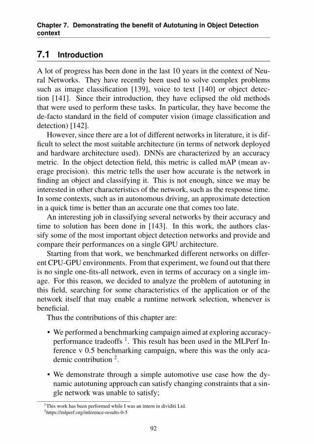
Chapter 7. Demonstrating the benefit of Autotuning in Object Detectioncontext
7.1 Introduction
A lot of progress has been done in the last 10 years in the context of Neu-ral Networks. They have recently been used to solve complex problemssuch as image classification [139], voice to text [140] or object detec-tion [141]. Since their introduction, they have eclipsed the old methodsthat were used to perform these tasks. In particular, they have become thede-facto standard in the field of computer vision (image classification anddetection) [142].
However, since there are a lot of different networks in literature, it is dif-ficult to select the most suitable architecture (in terms of network deployedand hardware architecture used). DNNs are characterized by an accuracymetric. In the object detection field, this metric is called mAP (mean av-erage precision). this metric tells the user how accurate is the network infinding an object and classifying it. This is not enough, since we may beinterested in other characteristics of the network, such as the response time.In some contexts, such as in autonomous driving, an approximate detectionin a quick time is better than an accurate one that comes too late.
An interesting job in classifying several networks by their accuracy andtime to solution has been done in [143]. In this work, the authors clas-sify some of the most important object detection networks and provide andcompare their performances on a single GPU architecture.
Starting from that work, we benchmarked different networks on differ-ent CPU-GPU environments. From that experiment, we found out that thereis no single one-fits-all network, even in terms of accuracy on a single im-age. For this reason, we decided to analyze the problem of autotuning inthis field, searching for some characteristics of the application or of thenetwork itself that may enable a runtime network selection, whenever isbeneficial.
Thus the contributions of this chapter are:
• We performed a benchmarking campaign aimed at exploring accuracy-performance tradeoffs 1. This result has been used in the MLPerf In-ference v 0.5 benchmarking campaign, where this was the only aca-demic contribution 2.
• We demonstrate through a simple automotive use case how the dy-namic autotuning approach can satisfy changing constraints that a sin-gle network was unable to satisfy;
1This work has been performed while I was an intern in dividiti Ltd.2https://mlperf.org/inference-results-0-5
92
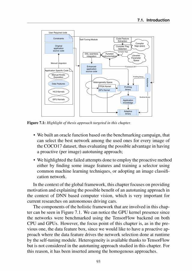
7.1. Introduction
User Required code
Self-Tuning Module
Heterogeneity Space
Originalapplication
source code
Code FeatureExtraction
Compilerflags space
Compiler flags
Compiler FlagSelection
Libraries Parameter
Space
DSL seamlessintegration
Enhancedapplication
source code
Profilingbinary
Applicationknowledge
Adaptivebinary
Runtime library
Framework API
Autotuner
Profiling library
Manual Integration
Application Specific Code
Data Features
HLS Kernels
GPU Kernels
FPGA Kernel
GPU Kernel
Constraints
Manual KnobsExposition
FunctionInstrumentation
Constraints Code FeatureExtraction
Compiler FlagSelection
FunctionInstrumentation Libraries
Parameter Space
Compilerflags space
DSL seamlessintegration
Autotuner
Figure 7.1: Highlight of thesis approach targeted in this chapter.
• We built an oracle function based on the benchmarking campaign, thatcan select the best network among the used ones for every image ofthe COCO17 dataset, thus evaluating the possible advantage in havinga proactive (per image) autotuning approach;
• We highlighted the failed attempts done to employ the proactive methodeither by finding some image features and training a selector usingcommon machine learning techniques, or adopting an image classifi-cation network.
In the context of the global framework, this chapter focuses on providingmotivation and explaining the possible benefit of an autotuning approach inthe context of DNN based computer vision, which is very important forcurrent researches on autonomous driving cars.
The components of the holistic framework that are involved in this chap-ter can be seen in Figure 7.1. We can notice the GPU kernel presence sincethe networks were benchmarked using the TensorFlow backend on bothCPU and GPUs. However, the focus point of this chapter is, as in the pre-vious one, the data feature box, since we would like to have a proactive ap-proach where the data feature drives the network selection done at runtimeby the self-tuning module. Heterogeneity is available thanks to TensorFlowbut is not considered in the autotuning approach studied in this chapter. Forthis reason, it has been inserted among the homogenous approaches.
93
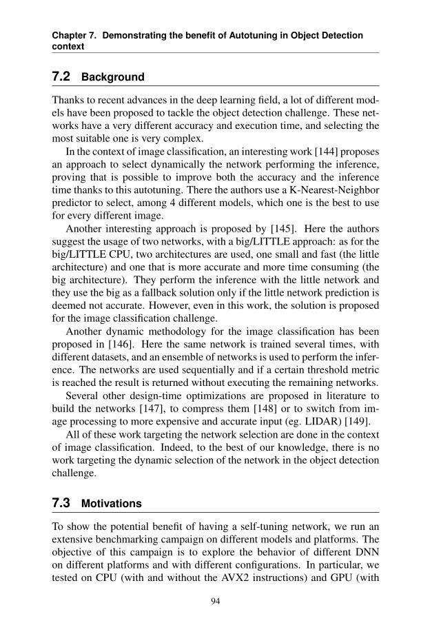
Chapter 7. Demonstrating the benefit of Autotuning in Object Detectioncontext
7.2 Background
Thanks to recent advances in the deep learning field, a lot of different mod-els have been proposed to tackle the object detection challenge. These net-works have a very different accuracy and execution time, and selecting themost suitable one is very complex.
In the context of image classification, an interesting work [144] proposesan approach to select dynamically the network performing the inference,proving that is possible to improve both the accuracy and the inferencetime thanks to this autotuning. There the authors use a K-Nearest-Neighborpredictor to select, among 4 different models, which one is the best to usefor every different image.
Another interesting approach is proposed by [145]. Here the authorssuggest the usage of two networks, with a big/LITTLE approach: as for thebig/LITTLE CPU, two architectures are used, one small and fast (the littlearchitecture) and one that is more accurate and more time consuming (thebig architecture). They perform the inference with the little network andthey use the big as a fallback solution only if the little network prediction isdeemed not accurate. However, even in this work, the solution is proposedfor the image classification challenge.
Another dynamic methodology for the image classification has beenproposed in [146]. Here the same network is trained several times, withdifferent datasets, and an ensemble of networks is used to perform the infer-ence. The networks are used sequentially and if a certain threshold metricis reached the result is returned without executing the remaining networks.
Several other design-time optimizations are proposed in literature tobuild the networks [147], to compress them [148] or to switch from im-age processing to more expensive and accurate input (eg. LIDAR) [149].
All of these work targeting the network selection are done in the contextof image classification. Indeed, to the best of our knowledge, there is nowork targeting the dynamic selection of the network in the object detectionchallenge.
7.3 Motivations
To show the potential benefit of having a self-tuning network, we run anextensive benchmarking campaign on different models and platforms. Theobjective of this campaign is to explore the behavior of different DNNon different platforms and with different configurations. In particular, wetested on CPU (with and without the AVX2 instructions) and GPU (with
94
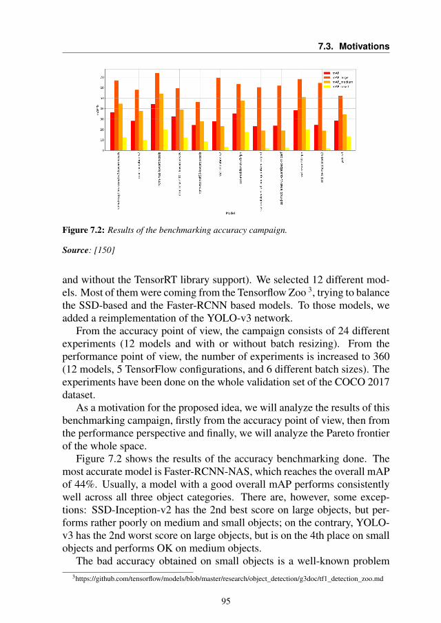
7.3. Motivations
Figure 7.2: Results of the benchmarking accuracy campaign.
Source: [150]
and without the TensorRT library support). We selected 12 different mod-els. Most of them were coming from the Tensorflow Zoo 3, trying to balancethe SSD-based and the Faster-RCNN based models. To those models, weadded a reimplementation of the YOLO-v3 network.
From the accuracy point of view, the campaign consists of 24 differentexperiments (12 models and with or without batch resizing). From theperformance point of view, the number of experiments is increased to 360(12 models, 5 TensorFlow configurations, and 6 different batch sizes). Theexperiments have been done on the whole validation set of the COCO 2017dataset.
As a motivation for the proposed idea, we will analyze the results of thisbenchmarking campaign, firstly from the accuracy point of view, then fromthe performance perspective and finally, we will analyze the Pareto frontierof the whole space.
Figure 7.2 shows the results of the accuracy benchmarking done. Themost accurate model is Faster-RCNN-NAS, which reaches the overall mAPof 44%. Usually, a model with a good overall mAP performs consistentlywell across all three object categories. There are, however, some excep-tions: SSD-Inception-v2 has the 2nd best score on large objects, but per-forms rather poorly on medium and small objects; on the contrary, YOLO-v3 has the 2nd worst score on large objects, but is on the 4th place on smallobjects and performs OK on medium objects.
The bad accuracy obtained on small objects is a well-known problem3https://github.com/tensorflow/models/blob/master/research/object_detection/g3doc/tf1_detection_zoo.md
95
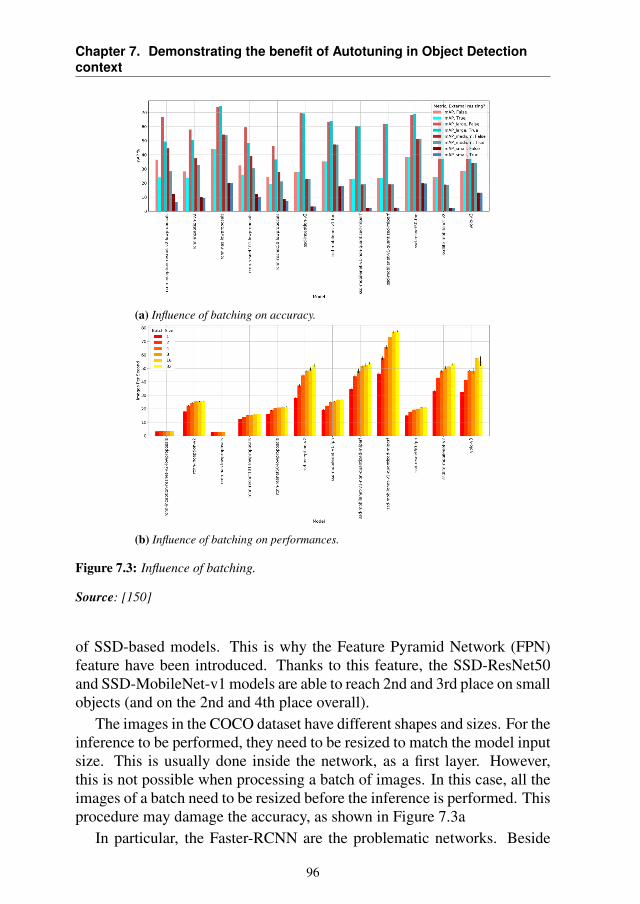
Chapter 7. Demonstrating the benefit of Autotuning in Object Detectioncontext
(a) Influence of batching on accuracy.
(b) Influence of batching on performances.
Figure 7.3: Influence of batching.
Source: [150]
of SSD-based models. This is why the Feature Pyramid Network (FPN)feature have been introduced. Thanks to this feature, the SSD-ResNet50and SSD-MobileNet-v1 models are able to reach 2nd and 3rd place on smallobjects (and on the 2nd and 4th place overall).
The images in the COCO dataset have different shapes and sizes. For theinference to be performed, they need to be resized to match the model inputsize. This is usually done inside the network, as a first layer. However,this is not possible when processing a batch of images. In this case, all theimages of a batch need to be resized before the inference is performed. Thisprocedure may damage the accuracy, as shown in Figure 7.3a
In particular, the Faster-RCNN are the problematic networks. Beside
96
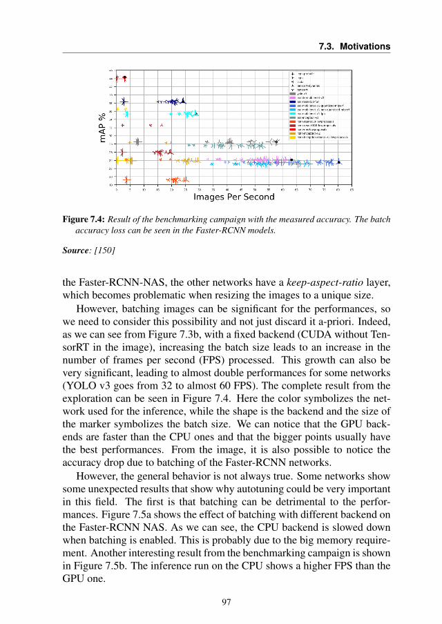
7.3. Motivations
Figure 7.4: Result of the benchmarking campaign with the measured accuracy. The batchaccuracy loss can be seen in the Faster-RCNN models.
Source: [150]
the Faster-RCNN-NAS, the other networks have a keep-aspect-ratio layer,which becomes problematic when resizing the images to a unique size.
However, batching images can be significant for the performances, sowe need to consider this possibility and not just discard it a-priori. Indeed,as we can see from Figure 7.3b, with a fixed backend (CUDA without Ten-sorRT in the image), increasing the batch size leads to an increase in thenumber of frames per second (FPS) processed. This growth can also bevery significant, leading to almost double performances for some networks(YOLO v3 goes from 32 to almost 60 FPS). The complete result from theexploration can be seen in Figure 7.4. Here the color symbolizes the net-work used for the inference, while the shape is the backend and the size ofthe marker symbolizes the batch size. We can notice that the GPU back-ends are faster than the CPU ones and that the bigger points usually havethe best performances. From the image, it is also possible to notice theaccuracy drop due to batching of the Faster-RCNN networks.
However, the general behavior is not always true. Some networks showsome unexpected results that show why autotuning could be very importantin this field. The first is that batching can be detrimental to the perfor-mances. Figure 7.5a shows the effect of batching with different backend onthe Faster-RCNN NAS. As we can see, the CPU backend is slowed downwhen batching is enabled. This is probably due to the big memory require-ment. Another interesting result from the benchmarking campaign is shownin Figure 7.5b. The inference run on the CPU shows a higher FPS than theGPU one.
97
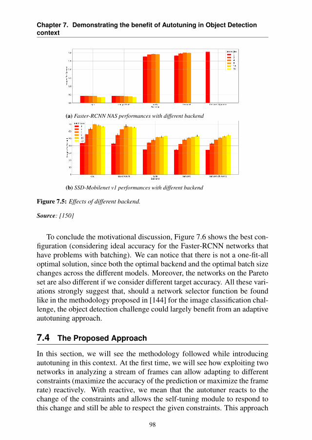
Chapter 7. Demonstrating the benefit of Autotuning in Object Detectioncontext
(a) Faster-RCNN NAS performances with different backend
(b) SSD-Mobilenet v1 performances with different backend
Figure 7.5: Effects of different backend.
Source: [150]
To conclude the motivational discussion, Figure 7.6 shows the best con-figuration (considering ideal accuracy for the Faster-RCNN networks thathave problems with batching). We can notice that there is not a one-fit-alloptimal solution, since both the optimal backend and the optimal batch sizechanges across the different models. Moreover, the networks on the Paretoset are also different if we consider different target accuracy. All these vari-ations strongly suggest that, should a network selector function be foundlike in the methodology proposed in [144] for the image classification chal-lenge, the object detection challenge could largely benefit from an adaptiveautotuning approach.
7.4 The Proposed Approach
In this section, we will see the methodology followed while introducingautotuning in this context. At the first time, we will see how exploiting twonetworks in analyzing a stream of frames can allow adapting to differentconstraints (maximize the accuracy of the prediction or maximize the framerate) reactively. With reactive, we mean that the autotuner reacts to thechange of the constraints and allows the self-tuning module to respond tothis change and still be able to respect the given constraints. This approach
98
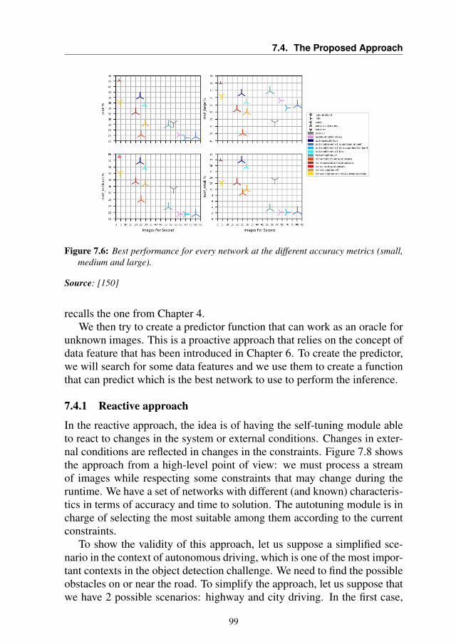
7.4. The Proposed Approach
Figure 7.6: Best performance for every network at the different accuracy metrics (small,medium and large).
Source: [150]
recalls the one from Chapter 4.We then try to create a predictor function that can work as an oracle for
unknown images. This is a proactive approach that relies on the concept ofdata feature that has been introduced in Chapter 6. To create the predictor,we will search for some data features and we use them to create a functionthat can predict which is the best network to use to perform the inference.
7.4.1 Reactive approach
In the reactive approach, the idea is of having the self-tuning module ableto react to changes in the system or external conditions. Changes in exter-nal conditions are reflected in changes in the constraints. Figure 7.8 showsthe approach from a high-level point of view: we must process a streamof images while respecting some constraints that may change during theruntime. We have a set of networks with different (and known) characteris-tics in terms of accuracy and time to solution. The autotuning module is incharge of selecting the most suitable among them according to the currentconstraints.
To show the validity of this approach, let us suppose a simplified sce-nario in the context of autonomous driving, which is one of the most impor-tant contexts in the object detection challenge. We need to find the possibleobstacles on or near the road. To simplify the approach, let us suppose thatwe have 2 possible scenarios: highway and city driving. In the first case,
99

Chapter 7. Demonstrating the benefit of Autotuning in Object Detectioncontext
(a) Execution time for every frame.
(b) mAP of all categories
(c) mAP of the car category
Figure 7.7: Execution log of the same stream with the two different networks, with achange of network in the middle.
we need to have a quick response and we need to identify "big" objects suchas cars, while in the second case we have a slower speed, which means thatwe can use a slower network but we require a greater accuracy since weneed to identify the "small" pedestrians.
In this simplified example, the autotuner is in charge of switching fromcontext 1 (city driving) to context 2 (highway) and back whenever a thresh-old speed is passed. For this experiment, we have used the KITTI dataset[151], which is a dataset created for the autonomous driving context. Asthe first network (the fast one for the highway context), we retrained theSSDLite-Mobilenet, while as the accurate network we retrained the Faster-RCNN NAS network.
We show in Figure 7.7 an example of a run where we hypothesize tostart the trip inside the city, where the most accurate network is used, and
100
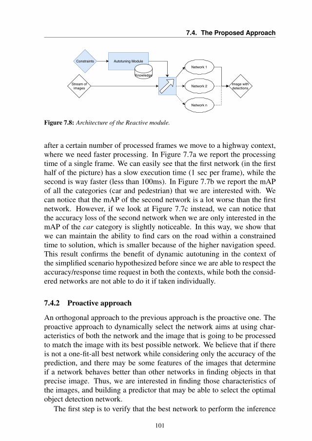
7.4. The Proposed Approach
Autotuning Module
Stream ofimages Network 2
Network n
Image withdetections
Network 1Constraints
Knowledge
Figure 7.8: Architecture of the Reactive module.
after a certain number of processed frames we move to a highway context,where we need faster processing. In Figure 7.7a we report the processingtime of a single frame. We can easily see that the first network (in the firsthalf of the picture) has a slow execution time (1 sec per frame), while thesecond is way faster (less than 100ms). In Figure 7.7b we report the mAPof all the categories (car and pedestrian) that we are interested with. Wecan notice that the mAP of the second network is a lot worse than the firstnetwork. However, if we look at Figure 7.7c instead, we can notice thatthe accuracy loss of the second network when we are only interested in themAP of the car category is slightly noticeable. In this way, we show thatwe can maintain the ability to find cars on the road within a constrainedtime to solution, which is smaller because of the higher navigation speed.This result confirms the benefit of dynamic autotuning in the context ofthe simplified scenario hypothesized before since we are able to respect theaccuracy/response time request in both the contexts, while both the consid-ered networks are not able to do it if taken individually.
7.4.2 Proactive approach
An orthogonal approach to the previous approach is the proactive one. Theproactive approach to dynamically select the network aims at using char-acteristics of both the network and the image that is going to be processedto match the image with its best possible network. We believe that if thereis not a one-fit-all best network while considering only the accuracy of theprediction, and there may be some features of the images that determineif a network behaves better than other networks in finding objects in thatprecise image. Thus, we are interested in finding those characteristics ofthe images, and building a predictor that may be able to select the optimalobject detection network.
The first step is to verify that the best network to perform the inference
101
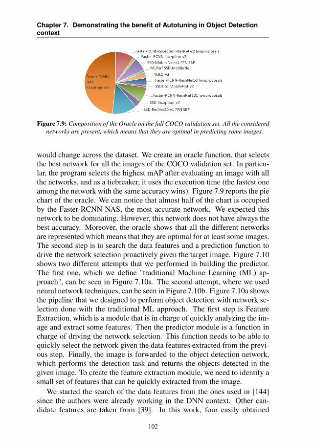
Chapter 7. Demonstrating the benefit of Autotuning in Object Detectioncontext
Figure 7.9: Composition of the Oracle on the full COCO validation set. All the considerednetworks are present, which means that they are optimal in predicting some images.
would change across the dataset. We create an oracle function, that selectsthe best network for all the images of the COCO validation set. In particu-lar, the program selects the highest mAP after evaluating an image with allthe networks, and as a tiebreaker, it uses the execution time (the fastest oneamong the network with the same accuracy wins). Figure 7.9 reports the piechart of the oracle. We can notice that almost half of the chart is occupiedby the Faster-RCNN NAS, the most accurate network. We expected thisnetwork to be dominating. However, this network does not have always thebest accuracy. Moreover, the oracle shows that all the different networksare represented which means that they are optimal for at least some images.The second step is to search the data features and a prediction function todrive the network selection proactively given the target image. Figure 7.10shows two different attempts that we performed in building the predictor.The first one, which we define "traditional Machine Learning (ML) ap-proach", can be seen in Figure 7.10a. The second attempt, where we usedneural network techniques, can be seen in Figure 7.10b. Figure 7.10a showsthe pipeline that we designed to perform object detection with network se-lection done with the traditional ML approach. The first step is FeatureExtraction, which is a module that is in charge of quickly analyzing the im-age and extract some features. Then the predictor module is a function incharge of driving the network selection. This function needs to be able toquickly select the network given the data features extracted from the previ-ous step. Finally, the image is forwarded to the object detection network,which performs the detection task and returns the objects detected in thegiven image. To create the feature extraction module, we need to identify asmall set of features that can be quickly extracted from the image.
We started the search of the data features from the ones used in [144]since the authors were already working in the DNN context. Other can-didate features are taken from [39]. In this work, four easily obtained
102
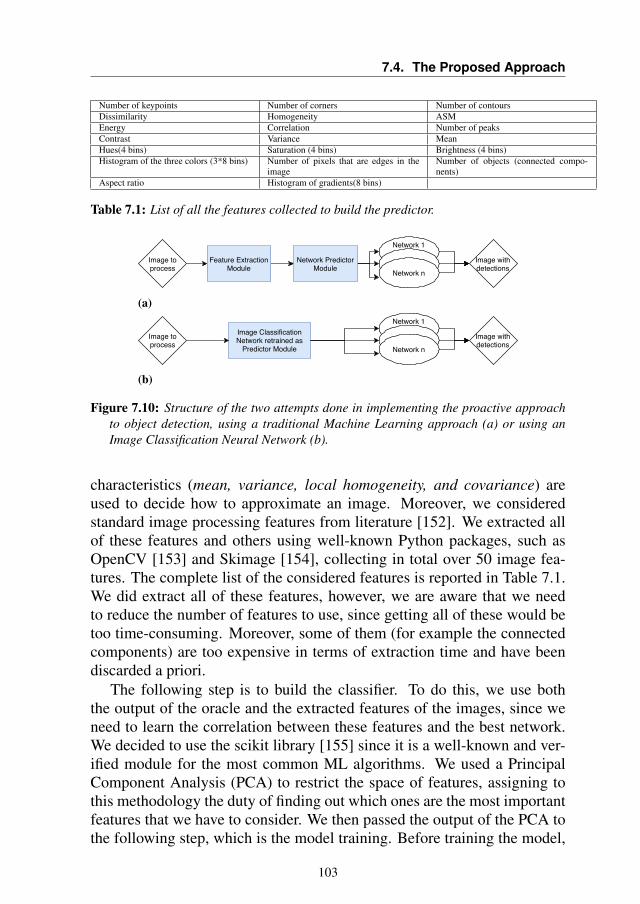
7.4. The Proposed Approach
Number of keypoints Number of corners Number of contoursDissimilarity Homogeneity ASMEnergy Correlation Number of peaksContrast Variance MeanHues(4 bins) Saturation (4 bins) Brightness (4 bins)Histogram of the three colors (3*8 bins) Number of pixels that are edges in the
imageNumber of objects (connected compo-nents)
Aspect ratio Histogram of gradients(8 bins)
Table 7.1: List of all the features collected to build the predictor.
Feature ExtractionModule
Image toprocess
Network PredictorModule
Network 1
Network n
Image withdetections
(a)
Image ClassificationNetwork retrained as
Predictor ModuleImage toprocess
Network 1
Network n
Image withdetections
(b)
Figure 7.10: Structure of the two attempts done in implementing the proactive approachto object detection, using a traditional Machine Learning approach (a) or using anImage Classification Neural Network (b).
characteristics (mean, variance, local homogeneity, and covariance) areused to decide how to approximate an image. Moreover, we consideredstandard image processing features from literature [152]. We extracted allof these features and others using well-known Python packages, such asOpenCV [153] and Skimage [154], collecting in total over 50 image fea-tures. The complete list of the considered features is reported in Table 7.1.We did extract all of these features, however, we are aware that we needto reduce the number of features to use, since getting all of these would betoo time-consuming. Moreover, some of them (for example the connectedcomponents) are too expensive in terms of extraction time and have beendiscarded a priori.
The following step is to build the classifier. To do this, we use boththe output of the oracle and the extracted features of the images, since weneed to learn the correlation between these features and the best network.We decided to use the scikit library [155] since it is a well-known and ver-ified module for the most common ML algorithms. We used a PrincipalComponent Analysis (PCA) to restrict the space of features, assigning tothis methodology the duty of finding out which ones are the most importantfeatures that we have to consider. We then passed the output of the PCA tothe following step, which is the model training. Before training the model,
103
Chapter 7. Demonstrating the benefit of Autotuning in Object Detectioncontext
we have to create the training and the test set. From the available 5000images (for which we have the array of features with the associated bestnetwork), we create a training set of 4500 images, while the other 500 areleft as validation set. Since the goal is to implement a classification layer,we have tested most of the classifier engines available in the scikit-learnmodule. Among them, we tested Decision Tree, Random Forest, Bagging,AdaBoost, Extra Trees, Gradient Boosting, SGD, MLP, KNeighbors. How-ever, no one of those algorithms was able to provide a robust classifier thatcould be used as the predictor, as we can notice from Figure 7.11. In par-ticular, Figure 7.11a shows the result on the complete set of networks. Inmost cases, the accuracy of the validation set was around 40% which isalso the number of occurrences of the most accurate model always (the lastcolumn in the figure). The tree predictor is the one that shows the worstresult, around 30%. To reduce the noise in the data available for the learn-ing phase, we restricted the number of models. We decided to use only theones that were Pareto optimal in the benchmarking study. This reduced thenumber of available models to 6. Nonetheless, even with the reduced num-ber of target networks, the traditional ML classifiers were unable to learnhow to predict the best network to use to perform object detection giventhe image. The result of this final experiment is reported in Figure 7.11b.We can notice that even with this reduction in the possible networks thereis no valid predictor: the last column (Faster-RCNN-NAS) is the predictorthat always selects the Faster-RCNN-NAS network to perform the detectionsince it is the most accurate one. This predictor has an accuracy of 55%,which means that in more than half of the test images the RCNN-NAS hasthe optimal accuracy in the reduced validation set. All the predictors havea worse result, meaning that they can guess the optimal network with lessaccuracy than always selecting the same, and most used, network.
Since the traditional approach did not lead us to a working solution forour problem, we decided to attempt using a DNN classifier. In particular,we selected a MobilenetV2, trained on the ImageNet dataset. We decided toperform transfer learning, thus only modifying the last layers (the classifierlayers) of the network, without changing the feature extraction layers. Thenetwork we used to perform the transfer learning has 154 frozen layers andthe last layer has 1280 features coming out, to which we attach the denselayers used to perform the classification. The total number of parametersof this network is 5,149,771, and more than half of them are frozen, so theycannot be trained during the transfer learning. As we can see, we have muchmore features than with the previous approach. We used the keras [156]framework to perform the transfer learning. Since the oracle shows that
104
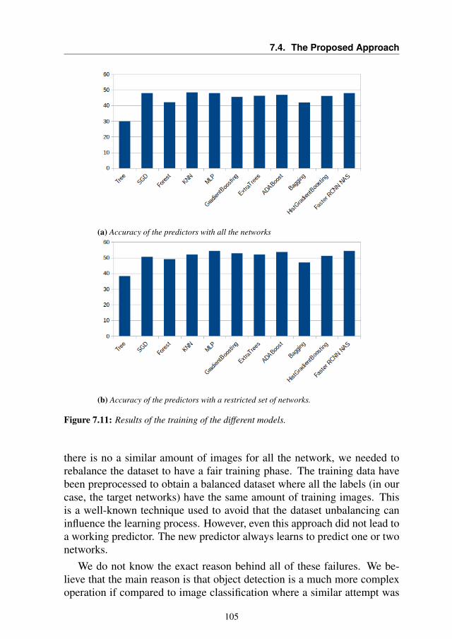
7.4. The Proposed Approach
(a) Accuracy of the predictors with all the networks
(b) Accuracy of the predictors with a restricted set of networks.
Figure 7.11: Results of the training of the different models.
there is no a similar amount of images for all the network, we needed torebalance the dataset to have a fair training phase. The training data havebeen preprocessed to obtain a balanced dataset where all the labels (in ourcase, the target networks) have the same amount of training images. Thisis a well-known technique used to avoid that the dataset unbalancing caninfluence the learning process. However, even this approach did not lead toa working predictor. The new predictor always learns to predict one or twonetworks.
We do not know the exact reason behind all of these failures. We be-lieve that the main reason is that object detection is a much more complexoperation if compared to image classification where a similar attempt was
105
Chapter 7. Demonstrating the benefit of Autotuning in Object Detectioncontext
successful [144]. Indeed, the DNN used to tackle this challenge are morecomplex than the classification networks: [143] shows how most object de-tection networks are composed of two sections, a region proposal networkthat aims at creating the bounding boxes of the objects, and a feature extrac-tor, which is an image classification network that provides the label to theobject extracted with the first stage. We think that this failure may be dueto the fact that the image features extracted with traditional image process-ing or with feature extraction layers trained for the classification problemare not enough. Indeed, these features may not be sufficient to model theregion proposal problem. Thus, a different set of features may be needed.
7.5 Summary
In this chapter, we have studied the possibility of applying autotuning in theobject detection context, where to the best of our knowledge has not beenalready attempted before. We have shown why the autotuning methodologycould be very profitable for this context, with a large benchmarking cam-paign that demonstrates that there is not a one-fit-all optimal solution. Wehave seen that using a reactive approach leads to benefits: we were able tosatisfy changing requirements by exploiting two networks that were unableto satisfy the given constraints if taken singularly. Even if our attempt inbuilding a working predictor was not successful, we believe that this canbe a motivational study that could inspire some researchers, more expert inthe DNN field, that this approach could be meaningful.
The outcome of this work has been accepted for publication to the SAMOS2021 international conference.
106
Part II
Geometric Docking case studies
107

CHAPTER8Background
In this secon half of the thesis we will describe some techiniques introducedon a molecular docking application called GeoDock. This application is akey component of this thesis, since half of the work that I did during myPh.D. was focused on improving the performance of this particular use case.
GeoDock is a component, in charge of geometric docking, of the Ligen[157] tool, which is itself a component in the EXSCALATE (EXaSCalesmArt pLatform Against paThogEns)1 tool-flow. This tool-flow is the in-silico section of a real drug discovery pipeline.
The goal of a drug discovery process is to find new drugs starting froma huge exploration space of candidate molecules. Typically, this processinvolves several in vivo, in vitro and in silico tasks ranging from chemicaldesign to toxicity analysis and in vivo experiments. Figure 8.1 shows thecomplete pipeline of a traditional drug discovery approach. We can no-tice that the virtual screening is a step in the exploratory research phase.Molecular docking represents but one stage of this step [158, 159]. It aimsat estimating the three-dimensional pose of a given molecule, named ligandwhen it interacts with the target protein. The ligand is much smaller thanthe target protein. For this reason, we only consider a region of the protein,
1https://www.exscalate.eu/en/platform.html
109
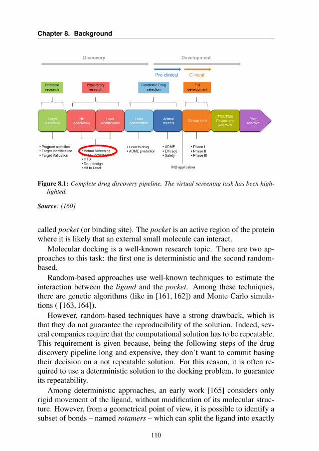
Chapter 8. Background
Figure 8.1: Complete drug discovery pipeline. The virtual screening task has been high-lighted.
Source: [160]
called pocket (or binding site). The pocket is an active region of the proteinwhere it is likely that an external small molecule can interact.
Molecular docking is a well-known research topic. There are two ap-proaches to this task: the first one is deterministic and the second random-based.
Random-based approaches use well-known techniques to estimate theinteraction between the ligand and the pocket. Among these techniques,there are genetic algorithms (like in [161, 162]) and Monte Carlo simula-tions ( [163, 164]).
However, random-based techniques have a strong drawback, which isthat they do not guarantee the reproducibility of the solution. Indeed, sev-eral companies require that the computational solution has to be repeatable.This requirement is given because, being the following steps of the drugdiscovery pipeline long and expensive, they don’t want to commit basingtheir decision on a not repeatable solution. For this reason, it is often re-quired to use a deterministic solution to the docking problem, to guaranteeits repeatability.
Among deterministic approaches, an early work [165] considers onlyrigid movement of the ligand, without modification of its molecular struc-ture. However, from a geometrical point of view, it is possible to identify asubset of bonds – named rotamers – which can split the ligand into exactly
110
two disjoint non-empty fragments when they are removed. Rotamers canindependently be rotated without changing the chemical connectivity of theligand. Therefore, most approaches evaluate also the changes in the shapeof the ligand that can be generated from the rotation of all its rotamers.For example, in [166] the molecular docking framework can deal with theflexibility of the ligand molecule by adopting a model of the electrostaticinteractions to finalize the docking. Similar works such as DOCK [167],FlexX [168], FlexX-Scan [169] and sur-flex [170] provide deterministicmolecular docking algorithms that are able to modify the shape of the lig-ands exploitintg the rotable bonds. These algorithms rely on both geomet-ric and pharmacophoric properties in their docking procedure. However,all these works implement a different docking procedure with respect toGeoDock.
From the computational point of view, the evaluation of each ligand isindependent of the evaluation of all the other candidates. This and the hugeamount of candidates to process makes this problem an embarrassingly par-allel one. Nonetheless, to find the optimal pose of the ligand when it inter-acts with the pocket, we still have to manage a large number of degreesof freedom, produced by the rotamers. To simplify the computation, thepocket is usually represented as a static structure, where the position of theatoms cannot change during the docking process. However, the ligand is aset of atoms connected by covalent bonds, i.e. atoms that share an electronpair. These atoms can move during the docking process and the shape ofthe ligand can change thanks to the rotation of the rotamers. Indeed, whilethe target pocket is represented as a rigid structure to simplify the compu-tation, the ligand is represented as a flexible set of atoms bound together bychemical bonds, i.e. sharing electron pairs between atoms (covalent bond).This makes the evaluation of the interactions between a single ligand andthe pocket from the chemical and physical perspective a computationally-intensive problem. For this reason, state of the art approaches [171–175]suggest separating the pose prediction task from the virtual screening task.These two tasks are very similar to each other in their organization: the firstone (pose prediction) focuses on finding the best positioning of a ligand ina pocket. The second one (virtual screening) aims at selecting a small set ofpromising ligands across a large dataset of candidates that maximize the fitto the given binding site. However, several industrial applications [163,176]perform both tasks into a single software module.
A fundamental difference between the pose prediction and the virtualscreening task lies in how the chemical and physical interactions betweenligand and pocket are used. Indeed, in the pose prediction task, it is possible
111
Chapter 8. Background
to estimate the position of the ligand without using them (geometrical ap-proach) or not (pharmacophoric approach). However, chemical informationis needed when performing the virtual screening. The pharmacophoric ap-proach is the most computational-intensive, while the geometric approachis more lightweight, thus faster. However, the best solution according toa pharmacophoric score implies a good geometrical score and a more ac-curate prediction. Indeed, there are no guarantees on the chemical com-patibility of the pocket-ligand pair when using the geometrical approach.The optimal solution obtained with a geometric approach may be eithera non-valid solution or a poor solution from a pharmacophoric perspec-tive. Therefore, it is mandatory to use pharmacophoric information whendoing the final selection. The geometrical approach may be useful to fil-ter among all the candidate ligands those that cannot geometrically fit thetarget pocket. This allows to perform the chemical scoring on an alreadyreduced set, thus speeding up the virtual screening process as a whole.
Nowadays, the amount of candidates evaluated with a virtual screen-ing pipeline is in recently reached 1 billion docked molecules on the entireSummit Supercomputer [177]. The objective of our research is to enable theexascale drug discovery paradigm, which can manage hundreds of billionsor trillions of candidate drugs. This can be obtained thanks to the speed-upin the first phase of the drug discovery process, the one performed throughcomputer simulations (in-silico). Indeed, having better docking perfor-mances allows testing more candidates. This can be obtained by applyingautotuning techniques to the algorithms, or exploiting the heterogeneity ofthe HPC facilities as we will see in the following chapters.
112
CHAPTER9Introducing Autotuning in GeoDock in a
Homogeneous Context
In this chapter, we studied the original monolithic GeoDock applicationto find optimization and autotuning opportunities. In particular, we ana-lyzed the algorithm to identify some application related software knobs,that allow applying the approximate computing paradigm. Those knobs re-lax constraints on the correctness of the result, allowing higher throughput.Moreover, we study that is possible to find a relation between the exposedtrade-offs and the input size. We exploit this relation to force a constrainton the time-to-solution, maximizing the output quality under this time con-straint. The output of this work is an initial tunable version of the applica-tion, although it is still running on the CPU only.
9.1 Introduction
During the virtual screening process, the time budget is an important con-straint that has to be considered when designing a screening campaign. Itis common practice to have a domain-expert human, whose job is to tunethe size of the database of molecules to dock according to the time budget.
113
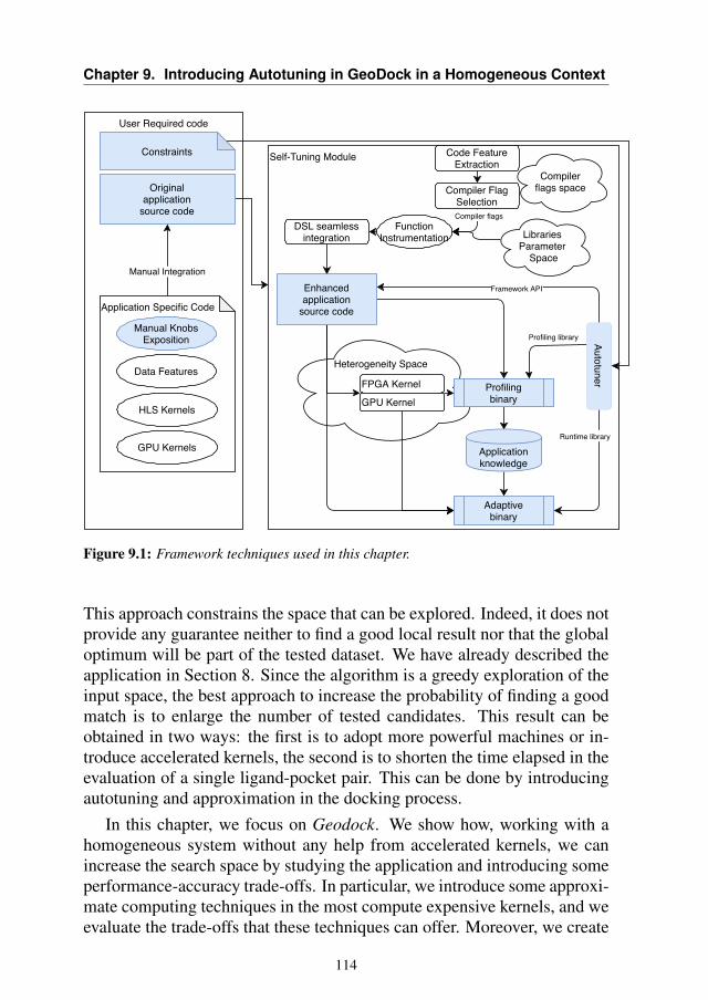
Chapter 9. Introducing Autotuning in GeoDock in a Homogeneous Context
User Required code
Self-Tuning Module
Heterogeneity Space
Originalapplication
source code
Code FeatureExtraction
Compilerflags space
Compiler flags
Compiler FlagSelection
Libraries Parameter
Space
DSL seamlessintegration
Enhancedapplication
source code
Profilingbinary
Applicationknowledge
Adaptivebinary
Runtime library
Framework API
Autotuner
Profiling library
Manual Integration
Application Specific Code
Data Features
HLS Kernels
GPU Kernels
FPGA Kernel
GPU Kernel
Constraints
Manual KnobsExposition
FunctionInstrumentation
Figure 9.1: Framework techniques used in this chapter.
This approach constrains the space that can be explored. Indeed, it does notprovide any guarantee neither to find a good local result nor that the globaloptimum will be part of the tested dataset. We have already described theapplication in Section 8. Since the algorithm is a greedy exploration of theinput space, the best approach to increase the probability of finding a goodmatch is to enlarge the number of tested candidates. This result can beobtained in two ways: the first is to adopt more powerful machines or in-troduce accelerated kernels, the second is to shorten the time elapsed in theevaluation of a single ligand-pocket pair. This can be done by introducingautotuning and approximation in the docking process.
In this chapter, we focus on Geodock. We show how, working with ahomogeneous system without any help from accelerated kernels, we canincrease the search space by studying the application and introducing someperformance-accuracy trade-offs. In particular, we introduce some approxi-mate computing techniques in the most compute expensive kernels, and weevaluate the trade-offs that these techniques can offer. Moreover, we create
114
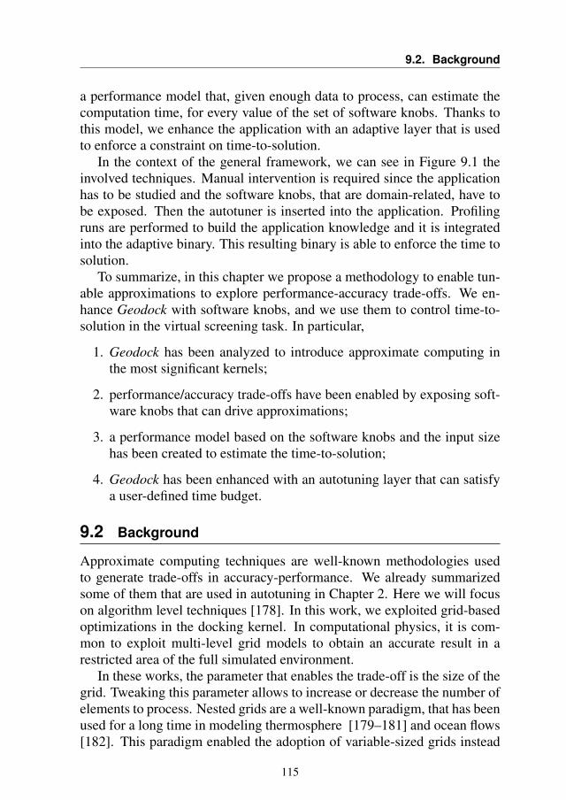
9.2. Background
a performance model that, given enough data to process, can estimate thecomputation time, for every value of the set of software knobs. Thanks tothis model, we enhance the application with an adaptive layer that is usedto enforce a constraint on time-to-solution.
In the context of the general framework, we can see in Figure 9.1 theinvolved techniques. Manual intervention is required since the applicationhas to be studied and the software knobs, that are domain-related, have tobe exposed. Then the autotuner is inserted into the application. Profilingruns are performed to build the application knowledge and it is integratedinto the adaptive binary. This resulting binary is able to enforce the time tosolution.
To summarize, in this chapter we propose a methodology to enable tun-able approximations to explore performance-accuracy trade-offs. We en-hance Geodock with software knobs, and we use them to control time-to-solution in the virtual screening task. In particular,
1. Geodock has been analyzed to introduce approximate computing inthe most significant kernels;
2. performance/accuracy trade-offs have been enabled by exposing soft-ware knobs that can drive approximations;
3. a performance model based on the software knobs and the input sizehas been created to estimate the time-to-solution;
4. Geodock has been enhanced with an autotuning layer that can satisfya user-defined time budget.
9.2 Background
Approximate computing techniques are well-known methodologies usedto generate trade-offs in accuracy-performance. We already summarizedsome of them that are used in autotuning in Chapter 2. Here we will focuson algorithm level techniques [178]. In this work, we exploited grid-basedoptimizations in the docking kernel. In computational physics, it is com-mon to exploit multi-level grid models to obtain an accurate result in arestricted area of the full simulated environment.
In these works, the parameter that enables the trade-off is the size of thegrid. Tweaking this parameter allows to increase or decrease the number ofelements to process. Nested grids are a well-known paradigm, that has beenused for a long time in modeling thermosphere [179–181] and ocean flows[182]. This paradigm enabled the adoption of variable-sized grids instead
115
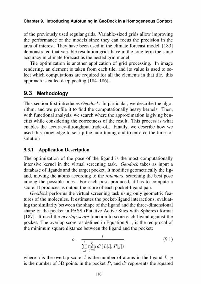
Chapter 9. Introducing Autotuning in GeoDock in a Homogeneous Context
of the previously used regular grids. Variable-sized grids allow improvingthe performance of the models since they can focus the precision in thearea of interest. They have been used in the climate forecast model. [183]demonstrated that variable resolution grids have in the long term the sameaccuracy in climate forecast as the nested grid model.
Tile optimization is another application of grid processing. In imagerendering, an element is taken from each tile, and its value is used to se-lect which computations are required for all the elements in that tile. thisapproach is called deep peeling [184–186].
9.3 Methodology
This section first introduces Geodock. In particular, we describe the algo-rithm, and we profile it to find the computationally heavy kernels. Then,with functional analysis, we search where the approximation is giving ben-efits while considering the correctness of the result. This process is whatenables the accuracy-throughput trade-off. Finally, we describe how weused this knowledge to set up the auto-tuning and to enforce the time-to-solution
9.3.1 Application Description
The optimization of the pose of the ligand is the most computationallyintensive kernel in the virtual screening task. Geodock takes as input adatabase of ligands and the target pocket. It modifies geometrically the lig-and, moving the atoms according to the rotamers, searching the best poseamong the possible ones. For each pose produced, it has to compute ascore. It produces as output the score of each pocket-ligand pair.
Geodock performs the virtual screening task using only geometric fea-tures of the molecules. It estimates the pocket-ligand interactions, evaluat-ing the similarity between the shape of the ligand and the three-dimensionalshape of the pocket in PASS (Putative Active Sites with Spheres) format[187]. It used the overlap score function to score each ligand against thepocket. The overlap score, as defined in Equation 9.1, is the reciprocal ofthe minimum square distance between the ligand and the pocket:
o =l
l∑i=0
p
minj=0
d2(L[i], P [j])
(9.1)
where o is the overlap score, l is the number of atoms in the ligand L, pis the number of 3D points in the pocket P , and d2 represents the squared
116
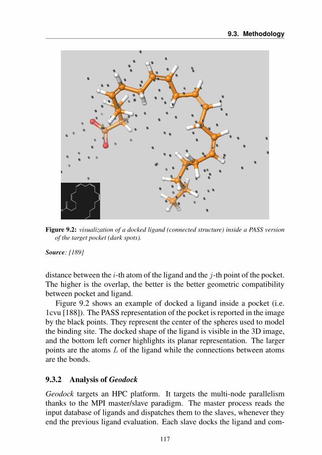
9.3. Methodology
Figure 9.2: visualization of a docked ligand (connected structure) inside a PASS versionof the target pocket (dark spots).
Source: [189]
distance between the i-th atom of the ligand and the j-th point of the pocket.The higher is the overlap, the better is the better geometric compatibilitybetween pocket and ligand.
Figure 9.2 shows an example of docked a ligand inside a pocket (i.e.1cvu [188]). The PASS representation of the pocket is reported in the imageby the black points. They represent the center of the spheres used to modelthe binding site. The docked shape of the ligand is visible in the 3D image,and the bottom left corner highlights its planar representation. The largerpoints are the atoms L of the ligand while the connections between atomsare the bonds.
9.3.2 Analysis of Geodock
Geodock targets an HPC platform. It targets the multi-node parallelismthanks to the MPI master/slave paradigm. The master process reads theinput database of ligands and dispatches them to the slaves, whenever theyend the previous ligand evaluation. Each slave docks the ligand and com-
117
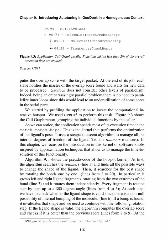
Chapter 9. Introducing Autotuning in GeoDock in a Homogeneous Context
99.9% - MPISlaveTask
98.7% - Molecule::MatchProbesShape
89.2% - Molecule::MeasureOverlap
08.2% - Fragment::CheckBumps
Figure 9.3: Application Call Graph profile. Functions taking less than 2% of the overallexecution time are omitted.
Source: [189]
putes the overlap score with the target pocket. At the end of its job, eachslave notifies the master of the overlap score found and waits for new datato be processed. Geodock does not consider other levels of parallelism.Indeed, being an embarrassingly parallel problem there is no need to paral-lelize inner loops since this would lead to an underutilization of some coresin the serial parts.
We started by profiling the application to locate the computational in-tensive hotspot. We used GPROF1 to perform this task. Figure 9.3 showsthe Call Graph report, grouping the individual functions by the caller.
As we can notice, the application spends most of its execution time in theMatchProbesShape. This is the kernel that performs the optimizationof the ligand’s pose. It uses a steepest descent algorithm to manage all theinternal degrees of freedom of the ligand (i.e. the rotamers rotations). Inthis chapter, we focus on the introduction in this kernel of software knobsinspired by approximation techniques that allow us to manage the time-to-solution of this functionality.
Algorithm 9.1 shows the pseudo-code of the hotspot kernel. At first,the algorithm searches the rotamers (line 1) and finds all the possible waysto change the shape of the ligand. Then, it searches for the best shapeby rotating the bonds one by one. (lines from 2 to 20). In particular, itgrows left and right ligand fragments, starting from the two extremes of thebond (line 3) and it rotates them independently. Every fragment is rotatedstep by step up to a 360 degree angle (lines from 4 to 5); At each step,we have to check whether the ligand shape is valid since there is a non-nullpossibility of internal bumping of the molecule. (line 6), If a bump is found,it invalidates that shape and we need to continue with the following rotationstep. If the ligand shape is valid, the algorithm computes the overlap scoreand checks if it is better than the previous score (lines from 7 to 9). At the
1GNU gprof https://sourceware.org/binutils/docs/gprof/
118
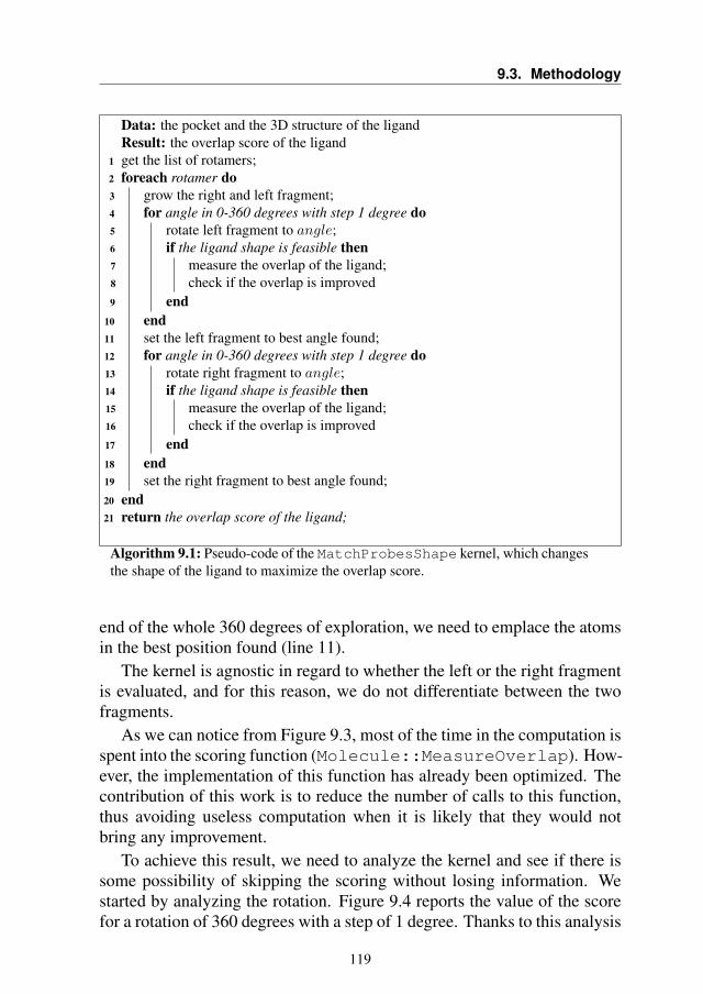
9.3. Methodology
Data: the pocket and the 3D structure of the ligandResult: the overlap score of the ligand
1 get the list of rotamers;2 foreach rotamer do3 grow the right and left fragment;4 for angle in 0-360 degrees with step 1 degree do5 rotate left fragment to angle;6 if the ligand shape is feasible then7 measure the overlap of the ligand;8 check if the overlap is improved9 end
10 end11 set the left fragment to best angle found;12 for angle in 0-360 degrees with step 1 degree do13 rotate right fragment to angle;14 if the ligand shape is feasible then15 measure the overlap of the ligand;16 check if the overlap is improved17 end18 end19 set the right fragment to best angle found;20 end21 return the overlap score of the ligand;
Algorithm 9.1: Pseudo-code of the MatchProbesShape kernel, which changesthe shape of the ligand to maximize the overlap score.
end of the whole 360 degrees of exploration, we need to emplace the atomsin the best position found (line 11).
The kernel is agnostic in regard to whether the left or the right fragmentis evaluated, and for this reason, we do not differentiate between the twofragments.
As we can notice from Figure 9.3, most of the time in the computation isspent into the scoring function (Molecule::MeasureOverlap). How-ever, the implementation of this function has already been optimized. Thecontribution of this work is to reduce the number of calls to this function,thus avoiding useless computation when it is likely that they would notbring any improvement.
To achieve this result, we need to analyze the kernel and see if there issome possibility of skipping the scoring without losing information. Westarted by analyzing the rotation. Figure 9.4 reports the value of the scorefor a rotation of 360 degrees with a step of 1 degree. Thanks to this analysis
119
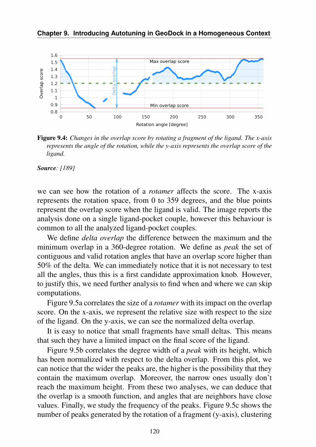
Chapter 9. Introducing Autotuning in GeoDock in a Homogeneous Context
0.8
0.9
1
1.1
1.2
1.3
1.4
1.5
1.6
0 50 100 150 200 250 300 350
Max overlap score
Min overlap score
Delt
a o
verl
ap
Overl
ap s
core
Rotation angle [degree]
Figure 9.4: Changes in the overlap score by rotating a fragment of the ligand. The x-axisrepresents the angle of the rotation, while the y-axis represents the overlap score of theligand.
Source: [189]
we can see how the rotation of a rotamer affects the score. The x-axisrepresents the rotation space, from 0 to 359 degrees, and the blue pointsrepresent the overlap score when the ligand is valid. The image reports theanalysis done on a single ligand-pocket couple, however this behaviour iscommon to all the analyzed ligand-pocket couples.
We define delta overlap the difference between the maximum and theminimum overlap in a 360-degree rotation. We define as peak the set ofcontiguous and valid rotation angles that have an overlap score higher than50% of the delta. We can immediately notice that it is not necessary to testall the angles, thus this is a first candidate approximation knob. However,to justify this, we need further analysis to find when and where we can skipcomputations.
Figure 9.5a correlates the size of a rotamer with its impact on the overlapscore. On the x-axis, we represent the relative size with respect to the sizeof the ligand. On the y-axis, we can see the normalized delta overlap.
It is easy to notice that small fragments have small deltas. This meansthat such they have a limited impact on the final score of the ligand.
Figure 9.5b correlates the degree width of a peak with its height, whichhas been normalized with respect to the delta overlap. From this plot, wecan notice that the wider the peaks are, the higher is the possibility that theycontain the maximum overlap. Moreover, the narrow ones usually don’treach the maximum height. From these two analyses, we can deduce thatthe overlap is a smooth function, and angles that are neighbors have closevalues. Finally, we study the frequency of the peaks. Figure 9.5c shows thenumber of peaks generated by the rotation of a fragment (y-axis), clustering
120
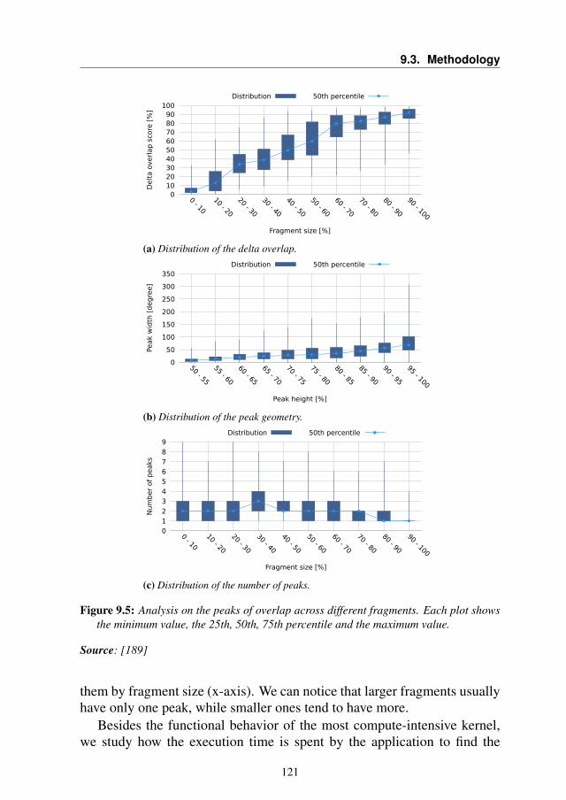
9.3. Methodology
0 10 20 30 40 50 60 70 80 90
100
0 - 10
10 - 20
20 - 30
30 - 40
40 - 50
50 - 60
60 - 70
70 - 80
80 - 90
90 - 100
Delt
a o
verl
ap s
core
[%
]
Fragment size [%]
Distribution 50th percentile
(a) Distribution of the delta overlap.
0
50
100
150
200
250
300
350
50 - 55
55 - 60
60 - 65
65 - 70
70 - 75
75 - 80
80 - 85
85 - 90
90 - 95
95 - 100
Peak
wid
th [
degre
e]
Peak height [%]
Distribution 50th percentile
(b) Distribution of the peak geometry.
0 1 2 3 4 5 6 7 8 9
0 - 10
10 - 20
20 - 30
30 - 40
40 - 50
50 - 60
60 - 70
70 - 80
80 - 90
90 - 100
Num
ber
of
peaks
Fragment size [%]
Distribution 50th percentile
(c) Distribution of the number of peaks.
Figure 9.5: Analysis on the peaks of overlap across different fragments. Each plot showsthe minimum value, the 25th, 50th, 75th percentile and the maximum value.
Source: [189]
them by fragment size (x-axis). We can notice that larger fragments usuallyhave only one peak, while smaller ones tend to have more.
Besides the functional behavior of the most compute-intensive kernel,we study how the execution time is spent by the application to find the
121
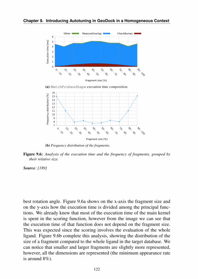
Chapter 9. Introducing Autotuning in GeoDock in a Homogeneous Context
0
1
2
3
4
5
6
0 - 10
10 - 20
20 - 30
30 - 40
40 - 50
50 - 60
60 - 70
70 - 80
80 - 90
90 - 100
Exe
cuti
on t
ime [
ms]
Fragment size [%]
Other MeasureOverlap CheckBumps
(a) MatchProbesShape execution time composition.
7
8
9
10
11
12
13
14
15
16
0 - 10
10 - 20
20 - 30
30 - 40
40 - 50
50 - 60
60 - 70
70 - 80
80 - 90
90 - 100
Frequency
dis
trib
uti
on [
%]
Fragment size [%]
(b) Frequency distribution of the fragments.
Figure 9.6: Analysis of the execution time and the frequency of fragments, grouped bytheir relative size.
Source: [189]
best rotation angle. Figure 9.6a shows on the x-axis the fragment size andon the y-axis how the execution time is divided among the principal func-tions. We already knew that most of the execution time of the main kernelis spent in the scoring function, however from the image we can see thatthe execution time of that function does not depend on the fragment size.This was expected since the scoring involves the evaluation of the wholeligand. Figure 9.6b complete this analysis, showing the distribution of thesize of a fragment compared to the whole ligand in the target database. Wecan notice that smaller and larger fragments are slightly more represented,however, all the dimensions are represented (the minimum appearance rateis around 8%).
122
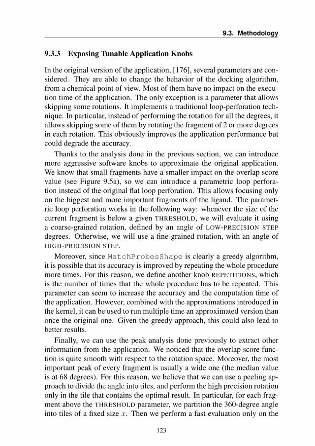
9.3. Methodology
9.3.3 Exposing Tunable Application Knobs
In the original version of the application, [176], several parameters are con-sidered. They are able to change the behavior of the docking algorithm,from a chemical point of view. Most of them have no impact on the execu-tion time of the application. The only exception is a parameter that allowsskipping some rotations. It implements a traditional loop-perforation tech-nique. In particular, instead of performing the rotation for all the degrees, itallows skipping some of them by rotating the fragment of 2 or more degreesin each rotation. This obviously improves the application performance butcould degrade the accuracy.
Thanks to the analysis done in the previous section, we can introducemore aggressive software knobs to approximate the original application.We know that small fragments have a smaller impact on the overlap scorevalue (see Figure 9.5a), so we can introduce a parametric loop perfora-tion instead of the original flat loop perforation. This allows focusing onlyon the biggest and more important fragments of the ligand. The paramet-ric loop perforation works in the following way: whenever the size of thecurrent fragment is below a given THRESHOLD, we will evaluate it usinga coarse-grained rotation, defined by an angle of LOW-PRECISION STEPdegrees. Otherwise, we will use a fine-grained rotation, with an angle ofHIGH-PRECISION STEP.
Moreover, since MatchProbesShape is clearly a greedy algorithm,it is possible that its accuracy is improved by repeating the whole proceduremore times. For this reason, we define another knob REPETITIONS, whichis the number of times that the whole procedure has to be repeated. Thisparameter can seem to increase the accuracy and the computation time ofthe application. However, combined with the approximations introduced inthe kernel, it can be used to run multiple time an approximated version thanonce the original one. Given the greedy approach, this could also lead tobetter results.
Finally, we can use the peak analysis done previously to extract otherinformation from the application. We noticed that the overlap score func-tion is quite smooth with respect to the rotation space. Moreover, the mostimportant peak of every fragment is usually a wide one (the median valueis at 68 degrees). For this reason, we believe that we can use a peeling ap-proach to divide the angle into tiles, and perform the high precision rotationonly in the tile that contains the optimal result. In particular, for each frag-ment above the THRESHOLD parameter, we partition the 360-degree angleinto tiles of a fixed size x. Then we perform a fast evaluation only on the
123
Chapter 9. Introducing Autotuning in GeoDock in a Homogeneous Context
0
0.2
0.4
0.6
0.8
1
0 50 100 150 200 250 300 350 0
50
100
150
200
250
300
350
400C
um
ula
tive p
rob
ab
ility
dis
trib
uti
on
Num
ber
of
evalu
ati
ons
Tile size [degrees]
Probability to find the highest peak in a fragmentEvaluations required to process a fragment
Proposed tile size
Figure 9.7: For each tile size (x-axis), the relation between the number of evaluated ro-tations (y2-axis) and the probability that the width of the best peak is greater than thegiven size (y1-axis).
Source: [189]
central element of each tile. In a second refinement, we examine the opti-mal tile with rotations of HIGH-PRECISION STEP degrees. With this tilingapproach, the number of evaluated rotations (y) is a function of the tile sizeand of the HIGH-PRECISION STEP parameter, as described in Equation 9.2
y =360◦
x+
x
HIGH-PRECISION STEP(9.2)
Since we want to minimize the computation effort while preserving theprobability of finding the best score, we minimize Equation 9.2. The solu-tion of this is reported in Equation 9.3.
x = 6 ∗√10 ∗√
HIGH-PRECISION STEP (9.3)
For example, if we set HIGH-PRECISION STEP at the original accuracy(1 degree), the optimal tile size is at 18 degrees. As we can see from Fig-ure 9.7, the probability of identifying the most important peak with thispeeling element is still well above 90%, which means that this approxima-tion is acceptable. Indeed, Figure 9.7 shows, for each tile size (x-axis), theprobability that the most important peak is wider than the evaluated tile size(y1-axis, blue line) and the number of evaluated iterations (y2-axis, greenline). The red line highlights the value obtained when minimizing the num-ber of evaluation with the proposed technique. As a consequence Equa-
124
9.3. Methodology
tion 9.3, we observe that a change in parameter HIGH-PRECISION STEPimplies a change in the value of the optimal tile size and in the probabilityof finding the best peak.
To summarize, starting from the original algorithm described in Algo-rithm 9.1, we introduced five tunable software-knobs: HIGH-PRECISIONSTEP, LOW-PRECISION STEP, THRESHOLD, REPETITIONS and ENABLEREFINEMENT, that enable approximation on the application and reduce thenumber of evaluations of the score function. The driving idea is that wewant to focus the elaboration only when it is required. And we try to avoiduseless computation thanks to the functional behavior analyzed in Subsec-tion 9.3.2.
To summarize, we report in Algorithm 9.2 the final parametric algorithmof MatchProbesShape. The outer loop (line 2) contains the originalalgorithm and consist of repeating the pose optimization according to REP-ETITIONS. The optimization of the pose is described for the left fragmentbetween line 5 and line 16. We test the relative size of the fragment againstthe THRESHOLD (line 5), to decide if perform either a coarse-grained ex-ploration or a fine-grained one. The coarse-grained exploration (line 6)uses the LOW-PRECISION STEP. The fine grained exploration (lines 9-15)is parametrized and has two possibilities. According to ENABLE REFINE-MENT, we can perform a two-step optimization using iterative refinements,or a flat exploration using HIGH-PRECISION STEP. The two-step optimiza-tion is done with the peeling technique that we explained before. We eval-uate the peeling elements of the rotation (line 10), then we refine the explo-ration of the most promising tile using HIGH-PRECISION STEP (line 11).Again, thanks to the symmetry of the problem, the procedure is applied tothe right fragment (lines 17-28) in the same way.
9.3.4 Application Autotuning
The software knobs defined aim at decreasing the time-to-solution of theapplication. However, as a side-effect, they also reduce the accuracy ofthe results. From the end-user point of view, a manual selection of theseparameters is not an easy task. Therefore we use the mARGOt autotun-ing framework to autotune the application and select the software-knobsconfiguration that maximizes the accuracy given a time budget.
The autotuner requires knowledge about the application behavior in or-der to select the most suitable configuration. There are two types of infor-mation needed by mARGOt to build the knowledge for this application:
1. Platform Independent knowledge, related to the error introduced with
125
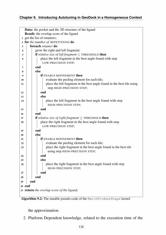
Chapter 9. Introducing Autotuning in GeoDock in a Homogeneous Context
Data: the pocket and the 3D structure of the ligandResult: the overlap score of the ligand
1 get the list of rotamers;2 for the number of REPETITIONS do3 foreach rotamer do4 grow the right and left fragment;5 if relative size of left fragment ≤ THRESHOLD then6 place the left fragment in the best angle found with step
LOW-PRECISION STEP;7 end8 else9 if ENABLE REFINEMENT then
10 evaluate the peeling element for each tile;11 place the left fragment in the best angle found in the best tile using
step HIGH-PRECISION STEP;12 end13 else14 place the left fragment in the best angle found with step
HIGH-PRECISION STEP;15 end16 end17 if relative size of right fragment ≤ THRESHOLD then18 place the right fragment in the best angle found with step
LOW-PRECISION STEP;19 end20 else21 if ENABLE REFINEMENT then22 evaluate the peeling element for each tile;23 place the right fragment in the best angle found in the best tile
using step HIGH-PRECISION STEP;24 end25 else26 place the right fragment in the best angle found with step
HIGH-PRECISION STEP;27 end28 end29 end30 end31 return the overlap score of the ligand;
Algorithm 9.2: The tunable pseudo-code of the MatchProbesShape kernel.
the approximation.
2. Platform Dependent knowledge, related to the execution time of the
126
9.3. Methodology
application on the actual machine that is used.
The first knowledge can be obtained by running only once, on a represen-tative set of pocket and ligands, an experimental campaign. It is importantthat the set is large, in order to avoid bias. Once this knowledge is built, itcan be used in different runs and on different platforms, since the error onlydepends on the knobs related to the approximation of the application.
On the other hand, to enforce a time-to-solution constraint, we need toknow the execution time on the given platform and the input set before-hand. Given the architecture of the application, and since the problem isdata-parallel, the overhead introduced by the MPI synchronization is con-sidered negligible even when scaling on a supercomputer machine with alarge set of nodes. Therefore, assuming that those nodes are homogeneous,we predict the time on the serial application and split it according to thenumber of available resources.
Considering a single software-knobs configuration, it is possible to usefeatures of the input database to estimate the time to solution. For thisreason, we model the entire database as a set of ligands with the same av-erage features. In particular, the model is built with a multivariate linearregression with interaction to estimate the time-to-solution tla for the aver-age ligand. The vector of predictors x is composed by the number of pointsof the target pocket xpp, the average number of atoms in a ligand xla, theaverage number of rotamers in a ligand xlr, and all the possible interactionsamong them (i.e. xpp · xla, xpp · xlr, xla · xlr, and xpp · xla · xlr). Thus, thetarget model is simply composed of tla = α · x + β, where α is the vectorof predictor coefficient, while β is the intercept.
To generalize this approach, we consider the parameters of the regres-sion as a function of the proposed software knobs. This is possible becausethe impact of the input on the execution time is strongly dependent on thesoftware-knobs configuration. Considering this, we can build a model toestimate the time-to-solution as stated in Equation 9.4. Here, k is the vec-tor of software knobs and ν is the number of ligands to dock, in the inputdatabase.
t = ν · (α(k) · x+ β(k)) (9.4)
As we already mentioned, we should train the performance model ev-ery time we change the computing platform. However, the experiment de-scribed in Subsection 9.5.1 characterize the size of the database required totrain the model.
To recap, we enhanced the original algorithm of the application finding
127
Chapter 9. Introducing Autotuning in GeoDock in a Homogeneous Context
and exposing software knobs, thus enabling performance-accuracy trade-offs. We used mARGOt to automatically configure the application requir-ing the user to provide only a couple of simple parameters, i.e. the numberof available nodes and the available time-budget. The characteristics of theactual input can be either provided by the user or extracted by a preliminaryinput analysis.
9.4 Experimental Setup
Before showing the benefit of the proposed approach, we need to define theboundaries of the experiment, in terms of dataset, metrics of interest, andexecution platform.
9.4.1 Data Sets
To evaluate the proposed methodology and its benefits, we used a databaseof 113K ligands.
The ligands were different both in terms of atoms (from 28 to 153) andin rotamers (from 2 to 53). Moreover, the order of the ligands inside thedataset is randomized, in order to remove bias due to their size.
We used 6 pockets protein pockets complexes derived from the RCSBProtein Data Bank (PDB) [188]: 1b9v, 1c1v, 1cvu, 1c2, 1dh3, 1fm9. In par-ticular, the PASS [187] version of the pockets has also been used togetherwith the database of ligands. The PASS version uses spheres to representbinding sites. This solution has been widely used in the context of fastdocking [187].
9.4.2 Metrics of Interest
The most important way to measure the performance of Geodock is to con-sider two metrics, the throughput (i.e. how many atoms per second it canevaluate) and, as previously said, the time to solution.
Now we need to identify a metric to estimate the error introduced bythe approximation. We call this metric overlap degradation. It is used toquantify the mean loss of accuracy introduced by approximation techniqueswith respect to the baseline. We consider as baseline the configuration thatleads, on average, to the better overlap score: HIGH-PRECISION STEP = 1◦,THRESHOLD = 0, REPETITIONS = 3 and ENABLE REFINEMENT = false.The overlap degradation is defined as described in Equation 9.5,
scoredegradation = (1− overlapapproxoverlaporiginal
)× 100 (9.5)
128

9.5. Experimental Results
where overlapapprox is the mean score of the top 1% of the ligands of theevaluated configuration, while overlaporiginal is the mean score of the top1% ligands of the baseline. Since this metrics evaluates the loss in accuracyof the approximated application, the lower it is its value, the closer is theapproximated application to the original one.
9.4.3 Target Platform
The platform used to execute the experiments is composed of two dedicatednodes of the supercomputer GALILEO, at the CINECA supercomputingcenter. Each node is equipped with two Intel Xeon E5-2630 V3 CPUs(@2.8 GHz) and 128 GB of DDR4 NUMA memory (@1866 MHz) on adual-channel memory configuration.
9.5 Experimental Results
In this section, we evaluate the benefits of the proposed approach usingfour different experiments. The first experiment is needed to evaluate thedata sensitivity. Geodock is a data-dependent application, so we want tofind out how many ligands are needed to stabilize the input sensitivity. Thismeans, how many ligands are needed to evaluate a configuration. The sec-ond experiment targets the approximation techniques. We want to show theenabled trade-off with respect to the baseline, evaluating the effect of thedegradation of the overlap score on a single ligand.
The third experiment validates the accuracy of the time-to-solution model.Finally, the fourth experiment shows the benefits of the proposed approach,in two different scenarios.
9.5.1 Data Dependency Evaluation
To evaluate the trade-off space, we need to find the set of Pareto optimalconfigurations, which are the configurations that are non-dominated con-sidering both target metrics (throughput and accuracy). However, this ap-plication needs to work with a database of ligands that is heterogeneous interms of the number of atoms and rotamers. Thus it is possible that theperformance and the input dataset are correlated, and that the applicationperformance depends on the input.
This experiment aims at finding the dependence of the performance ofthe configuration from the input dataset. If we manage to find its indepen-dence, we can avoid profiling the configuration behavior for every different
129
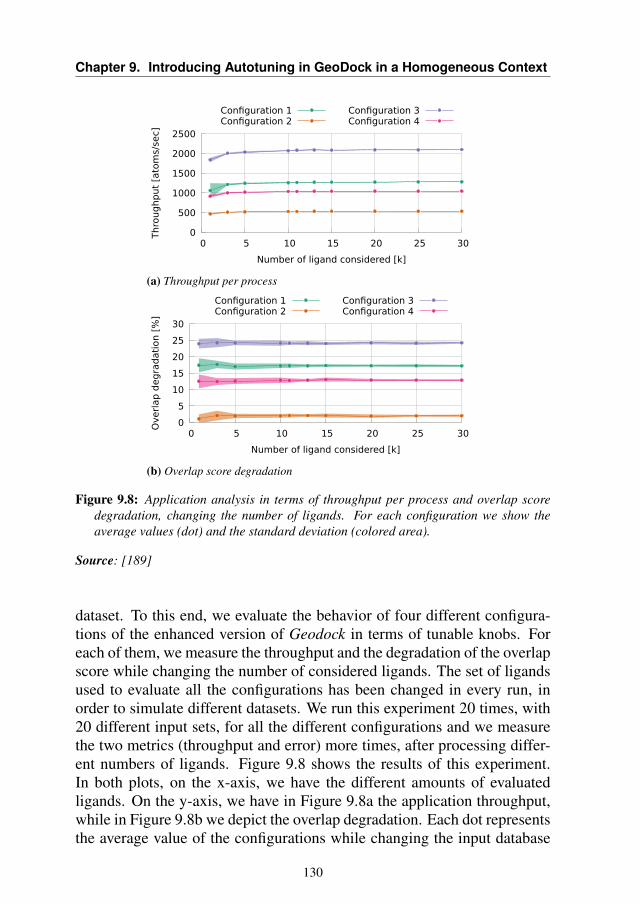
Chapter 9. Introducing Autotuning in GeoDock in a Homogeneous Context
0
500
1000
1500
2000
2500
0 5 10 15 20 25 30
Thro
ughput
[ato
ms/
sec]
Number of ligand considered [k]
Configuration 1Configuration 2
Configuration 3Configuration 4
(a) Throughput per process
0
5
10
15
20
25
30
0 5 10 15 20 25 30
Overl
ap d
egra
dati
on [
%]
Number of ligand considered [k]
Configuration 1Configuration 2
Configuration 3Configuration 4
(b) Overlap score degradation
Figure 9.8: Application analysis in terms of throughput per process and overlap scoredegradation, changing the number of ligands. For each configuration we show theaverage values (dot) and the standard deviation (colored area).
Source: [189]
dataset. To this end, we evaluate the behavior of four different configura-tions of the enhanced version of Geodock in terms of tunable knobs. Foreach of them, we measure the throughput and the degradation of the overlapscore while changing the number of considered ligands. The set of ligandsused to evaluate all the configurations has been changed in every run, inorder to simulate different datasets. We run this experiment 20 times, with20 different input sets, for all the different configurations and we measurethe two metrics (throughput and error) more times, after processing differ-ent numbers of ligands. Figure 9.8 shows the results of this experiment.In both plots, on the x-axis, we have the different amounts of evaluatedligands. On the y-axis, we have in Figure 9.8a the application throughput,while in Figure 9.8b we depict the overlap degradation. Each dot representsthe average value of the configurations while changing the input database
130
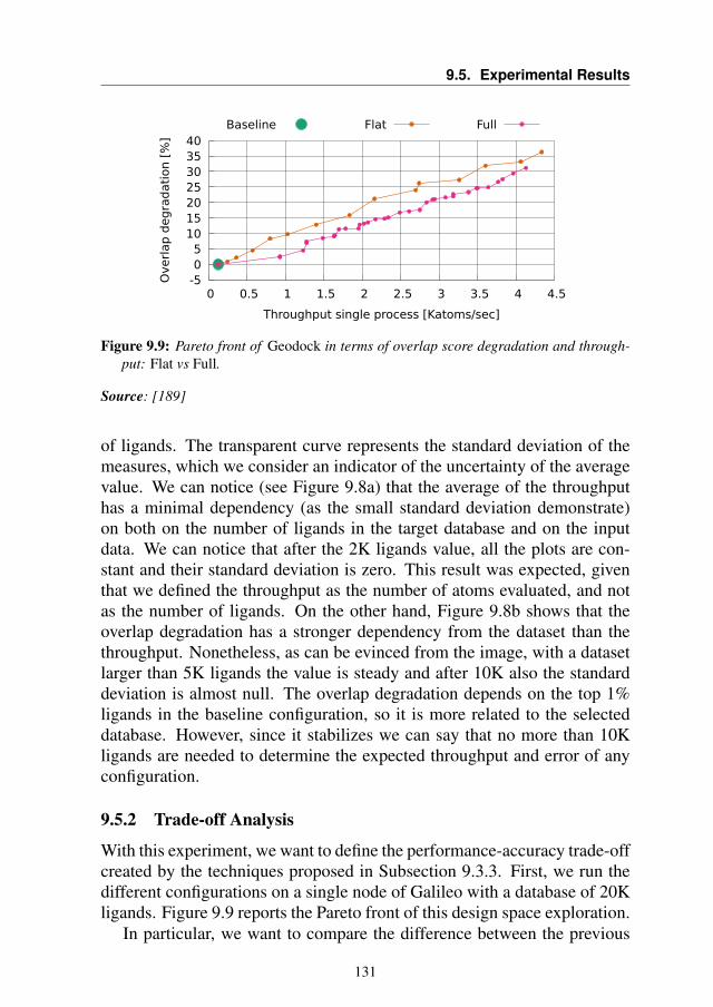
9.5. Experimental Results
-5 0 5
10 15 20 25 30 35 40
0 0.5 1 1.5 2 2.5 3 3.5 4 4.5
Overl
ap
deg
rad
ati
on [
%]
Throughput single process [Katoms/sec]
Baseline Flat Full
Figure 9.9: Pareto front of Geodock in terms of overlap score degradation and through-put: Flat vs Full.
Source: [189]
of ligands. The transparent curve represents the standard deviation of themeasures, which we consider an indicator of the uncertainty of the averagevalue. We can notice (see Figure 9.8a) that the average of the throughputhas a minimal dependency (as the small standard deviation demonstrate)on both on the number of ligands in the target database and on the inputdata. We can notice that after the 2K ligands value, all the plots are con-stant and their standard deviation is zero. This result was expected, giventhat we defined the throughput as the number of atoms evaluated, and notas the number of ligands. On the other hand, Figure 9.8b shows that theoverlap degradation has a stronger dependency from the dataset than thethroughput. Nonetheless, as can be evinced from the image, with a datasetlarger than 5K ligands the value is steady and after 10K also the standarddeviation is almost null. The overlap degradation depends on the top 1%ligands in the baseline configuration, so it is more related to the selecteddatabase. However, since it stabilizes we can say that no more than 10Kligands are needed to determine the expected throughput and error of anyconfiguration.
9.5.2 Trade-off Analysis
With this experiment, we want to define the performance-accuracy trade-offcreated by the techniques proposed in Subsection 9.3.3. First, we run thedifferent configurations on a single node of Galileo with a database of 20Kligands. Figure 9.9 reports the Pareto front of this design space exploration.
In particular, we want to compare the difference between the previous
131
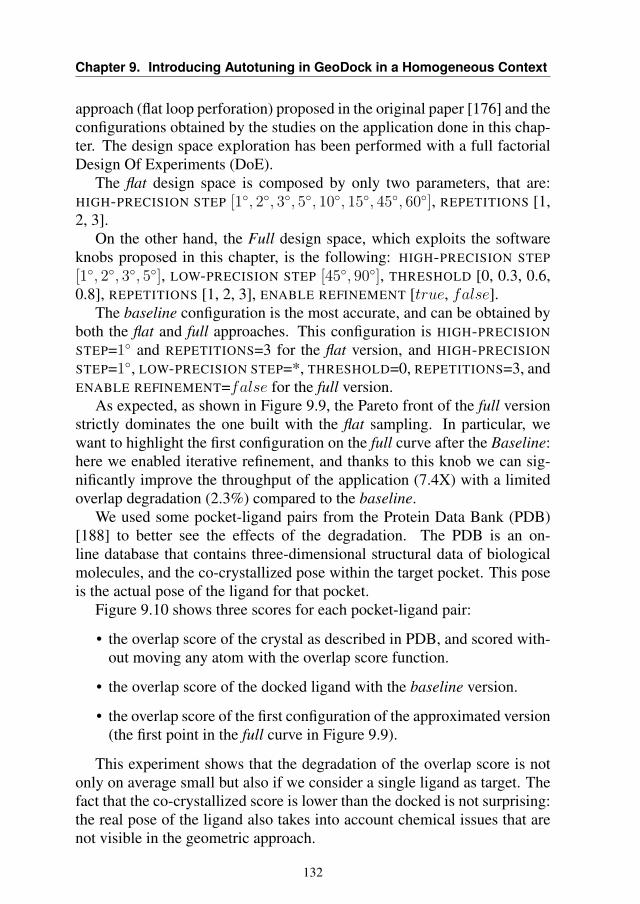
Chapter 9. Introducing Autotuning in GeoDock in a Homogeneous Context
approach (flat loop perforation) proposed in the original paper [176] and theconfigurations obtained by the studies on the application done in this chap-ter. The design space exploration has been performed with a full factorialDesign Of Experiments (DoE).
The flat design space is composed by only two parameters, that are:HIGH-PRECISION STEP [1◦, 2◦, 3◦, 5◦, 10◦, 15◦, 45◦, 60◦], REPETITIONS [1,2, 3].
On the other hand, the Full design space, which exploits the softwareknobs proposed in this chapter, is the following: HIGH-PRECISION STEP[1◦, 2◦, 3◦, 5◦], LOW-PRECISION STEP [45◦, 90◦], THRESHOLD [0, 0.3, 0.6,0.8], REPETITIONS [1, 2, 3], ENABLE REFINEMENT [true, false].
The baseline configuration is the most accurate, and can be obtained byboth the flat and full approaches. This configuration is HIGH-PRECISIONSTEP=1◦ and REPETITIONS=3 for the flat version, and HIGH-PRECISIONSTEP=1◦, LOW-PRECISION STEP=*, THRESHOLD=0, REPETITIONS=3, andENABLE REFINEMENT=false for the full version.
As expected, as shown in Figure 9.9, the Pareto front of the full versionstrictly dominates the one built with the flat sampling. In particular, wewant to highlight the first configuration on the full curve after the Baseline:here we enabled iterative refinement, and thanks to this knob we can sig-nificantly improve the throughput of the application (7.4X) with a limitedoverlap degradation (2.3%) compared to the baseline.
We used some pocket-ligand pairs from the Protein Data Bank (PDB)[188] to better see the effects of the degradation. The PDB is an on-line database that contains three-dimensional structural data of biologicalmolecules, and the co-crystallized pose within the target pocket. This poseis the actual pose of the ligand for that pocket.
Figure 9.10 shows three scores for each pocket-ligand pair:
• the overlap score of the crystal as described in PDB, and scored with-out moving any atom with the overlap score function.
• the overlap score of the docked ligand with the baseline version.
• the overlap score of the first configuration of the approximated version(the first point in the full curve in Figure 9.9).
This experiment shows that the degradation of the overlap score is notonly on average small but also if we consider a single ligand as target. Thefact that the co-crystallized score is lower than the docked is not surprising:the real pose of the ligand also takes into account chemical issues that arenot visible in the geometric approach.
132
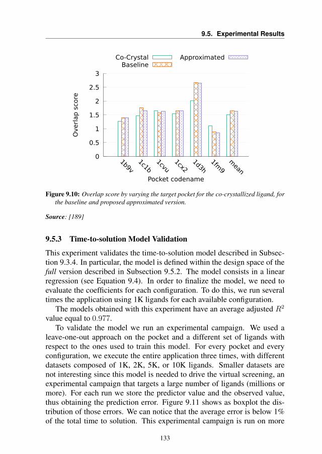
9.5. Experimental Results
0
0.5
1
1.5
2
2.5
3
1b9v1c1b
1cvu1cx2
1d3h1fm
9m
ean
Overl
ap
sco
re
Pocket codename
Co-CrystalBaseline
Approximated
Figure 9.10: Overlap score by varying the target pocket for the co-crystallized ligand, forthe baseline and proposed approximated version.
Source: [189]
9.5.3 Time-to-solution Model Validation
This experiment validates the time-to-solution model described in Subsec-tion 9.3.4. In particular, the model is defined within the design space of thefull version described in Subsection 9.5.2. The model consists in a linearregression (see Equation 9.4). In order to finalize the model, we need toevaluate the coefficients for each configuration. To do this, we run severaltimes the application using 1K ligands for each available configuration.
The models obtained with this experiment have an average adjusted R2
value equal to 0.977.To validate the model we run an experimental campaign. We used a
leave-one-out approach on the pocket and a different set of ligands withrespect to the ones used to train this model. For every pocket and everyconfiguration, we execute the entire application three times, with differentdatasets composed of 1K, 2K, 5K, or 10K ligands. Smaller datasets arenot interesting since this model is needed to drive the virtual screening, anexperimental campaign that targets a large number of ligands (millions ormore). For each run we store the predictor value and the observed value,thus obtaining the prediction error. Figure 9.11 shows as boxplot the dis-tribution of those errors. We can notice that the average error is below 1%of the total time to solution. This experimental campaign is run on more
133
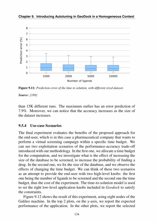
Chapter 9. Introducing Autotuning in GeoDock in a Homogeneous Context
0
1
2
3
4
5
6
7
8
1000 2000 5000 10000
Pre
dic
tion e
rror
[%]
Number of ligands
Figure 9.11: Prediction error of the time to solution, with different sized dataset.
Source: [189]
than 15K different runs. The maximum outlier has an error prediction of7.9%. Moreover, we can notice that the accuracy increases as the size ofthe dataset increases.
9.5.4 Use-case Scenarios
The final experiment evaluates the benefits of the proposed approach forthe end-user, which is in this case a pharmaceutical company that wants toperform a virtual screening campaign within a specific time budget. Wecan see two exploitation scenarios of the performance-accuracy trade-offintroduced with our methodology. In the first one, we allocate a time budgetfor the computation, and we investigate what is the effect of increasing thesize of the database to be screened, to increase the probability of finding adrug. In the second one, we fix the size of the database, and we observe theeffects of changing the time budget. We can think of these two scenariosas an attempt to provide the end-user with two high-level knobs: the firstone being the number of ligands to be screened and the second one the timebudget, thus the cost of the experiment. The time-to-solution model is usedto set the right low-level application knobs included in Geodock to satisfythe constraints.
Figure 9.12 shows the result of this experiment, using eight nodes of theGalileo machine. In the top 2 plots, on the y-axis, we report the expectedperformance of the application. In the other plots, we report the selected
134
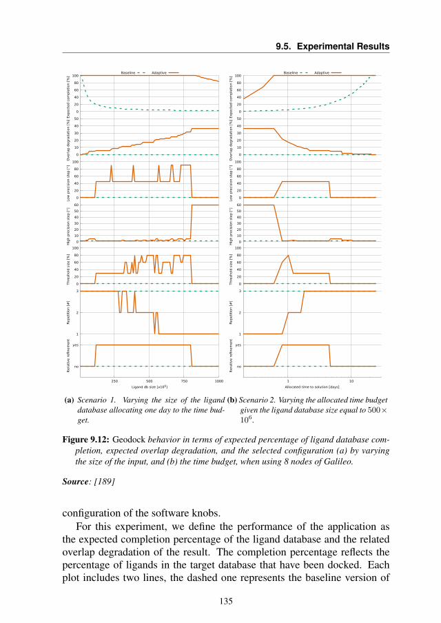
9.5. Experimental Results
0
20
40
60
80
100
Expect
ed c
om
ple
tion [
%]
Baseline Adaptive
0
10
20
30
40
50
Overl
ap d
egra
dati
on [
%]
0
20
40
60
80
100
Low
pre
cisi
on s
tep [
°]
0
10
20
30
40
50
60
Hig
h p
reci
sion s
tep [
°]
0
20
40
60
80
100
Thre
shold
siz
e [
%]
1
2
3
Repeti
tion [
#]
no
yes
250 500 750 1000
Itera
tive r
efinem
ent
Ligand db size [x106]
(a) Scenario 1. Varying the size of the liganddatabase allocating one day to the time bud-get.
0
20
40
60
80
100
Expect
ed c
om
ple
tion [
%]
Baseline Adaptive
0
10
20
30
40
50
Overl
ap d
egra
dati
on [
%]
0
20
40
60
80
100
Low
pre
cisi
on s
tep [
°]
0
10
20
30
40
50
60
Hig
h p
reci
sion s
tep [
°]
0
20
40
60
80
100
Thre
shold
siz
e [
%]
1
2
3
Repeti
tion [
#]
no
yes
1 10
Itera
tive r
efinem
ent
Allocated time to solution [days]
(b) Scenario 2. Varying the allocated time budgetgiven the ligand database size equal to 500×106.
Figure 9.12: Geodock behavior in terms of expected percentage of ligand database com-pletion, expected overlap degradation, and the selected configuration (a) by varyingthe size of the input, and (b) the time budget, when using 8 nodes of Galileo.
Source: [189]
configuration of the software knobs.For this experiment, we define the performance of the application as
the expected completion percentage of the ligand database and the relatedoverlap degradation of the result. The completion percentage reflects thepercentage of ligands in the target database that have been docked. Eachplot includes two lines, the dashed one represents the baseline version of
135
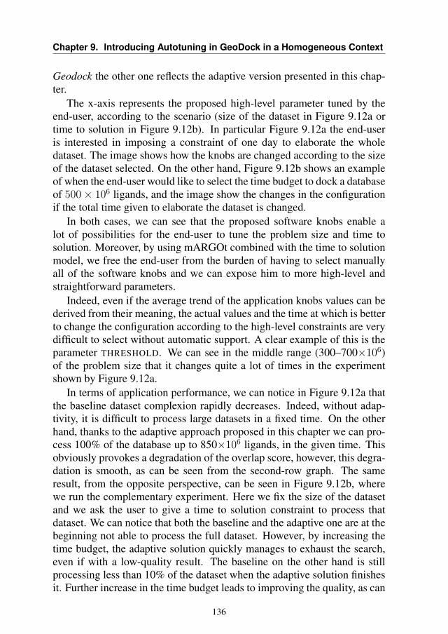
Chapter 9. Introducing Autotuning in GeoDock in a Homogeneous Context
Geodock the other one reflects the adaptive version presented in this chap-ter.
The x-axis represents the proposed high-level parameter tuned by theend-user, according to the scenario (size of the dataset in Figure 9.12a ortime to solution in Figure 9.12b). In particular Figure 9.12a the end-useris interested in imposing a constraint of one day to elaborate the wholedataset. The image shows how the knobs are changed according to the sizeof the dataset selected. On the other hand, Figure 9.12b shows an exampleof when the end-user would like to select the time budget to dock a databaseof 500× 106 ligands, and the image show the changes in the configurationif the total time given to elaborate the dataset is changed.
In both cases, we can see that the proposed software knobs enable alot of possibilities for the end-user to tune the problem size and time tosolution. Moreover, by using mARGOt combined with the time to solutionmodel, we free the end-user from the burden of having to select manuallyall of the software knobs and we can expose him to more high-level andstraightforward parameters.
Indeed, even if the average trend of the application knobs values can bederived from their meaning, the actual values and the time at which is betterto change the configuration according to the high-level constraints are verydifficult to select without automatic support. A clear example of this is theparameter THRESHOLD. We can see in the middle range (300–700×106)of the problem size that it changes quite a lot of times in the experimentshown by Figure 9.12a.
In terms of application performance, we can notice in Figure 9.12a thatthe baseline dataset complexion rapidly decreases. Indeed, without adap-tivity, it is difficult to process large datasets in a fixed time. On the otherhand, thanks to the adaptive approach proposed in this chapter we can pro-cess 100% of the database up to 850×106 ligands, in the given time. Thisobviously provokes a degradation of the overlap score, however, this degra-dation is smooth, as can be seen from the second-row graph. The sameresult, from the opposite perspective, can be seen in Figure 9.12b, wherewe run the complementary experiment. Here we fix the size of the datasetand we ask the user to give a time to solution constraint to process thatdataset. We can notice that both the baseline and the adaptive one are at thebeginning not able to process the full dataset. However, by increasing thetime budget, the adaptive solution quickly manages to exhaust the search,even if with a low-quality result. The baseline on the other hand is stillprocessing less than 10% of the dataset when the adaptive solution finishesit. Further increase in the time budget leads to improving the quality, as can
136
9.6. Summary
be seen in the second-row graph. It is interesting to note that the adaptivesolution can exhaust the dataset in less than 1 day, with less than 40% ofdegradation, while the baseline is still stuck at less than 10%, and requiresmore than 20 days to finish the run.
Finally, this experiment shows how the adaptive approach can providean output with a limited overlap degradation (less than 10%), while thebaseline can process only the 10% of input data set (Figure 9.12b, more orless at 2 days of run time). This result demonstrates the effectiveness of theextracted low-level knobs in Geodock.
9.6 Summary
In this chapter, we have analyzed Geodock as a representative HPC ap-plication. From the analysis of the application and domain knowledge, wewere able to identify five software-knobs that enable accuracy-performancetrade-offs, by focusing the computation where it is really useful and has animpact on the output value. The adaptive version of Geodock is charac-terized by different levels of accuracy, that are automatically managed bymARGOt according to the needs of the end-user of the virtual screeningexperimental campaign. In particular, experimental results demonstratedhow, by scaling the quality of the results, the application is able to completea virtual screening campaign over a given ligand database, with differenttime budgets. These results are an important advantage for pharmaceuticalcompanies where the usage of software and HPC systems have become animportant asset in the search for novel drugs. Due to the large number ofpossible molecules to evaluate, the proposed approach can either lower thecost of the virtual screening process or allow to evaluate a larger number ofligands, thus increasing the chances of finding a good candidate drug.
The analysis derived from the work presented in this chapter has beenused to optimize and tune a very large virtual screening run on the wholeMARCONI machine from CINECA (>250Kcores, >10PetaFlops system).When this work has been done, this machine was at position number 17 onthe top 500. In particular, this experiment has performed one of the largestvirtual screening campaign for the ZIKA virus considering a database of1.2B ligands. The resulting candidates are currently under in-vitro and in-vivo testing.
The outcome of this work has been published in the Journal of Super-computing [189].
137

CHAPTER10Porting and Tuning Geodock kernels to
GPU using OpenACC
In this chapter, we focus on porting Geodock to a heterogeneous node,showing how it is possible to significantly improve computation efficiencyby using heterogeneous architecture. In this chapter, we will describe howwe analyzed and rewrote the application to match the GPU parallel archi-tecture, and we performed a minimal static autotuning to select, before therun, the optimal configuration for some GPU parameters. In this imple-mentation of GeoDock, we used the OpenACC language to implement theparallel kernels on the GPU.
10.1 Introduction
In the last decade, energy consumption has become an important issue alsoin the HPC domain. For this reason, a switch from homogeneous systemsto heterogeneous systems has begun. By using different hardware accelera-tors, such as GPUs or Xeon-phi, heterogeneous systems usually have betterenergy efficiency and can provide more FLOPs. Indeed, most of the toppositions in the Green500 list (as of June 2020, [2]) are occupied by het-
139
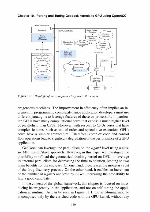
Chapter 10. Porting and Tuning Geodock kernels to GPU using OpenACC
User Required code
Self-Tuning Module
Heterogeneity Space
Originalapplication
source code
Code FeatureExtraction
Compilerflags space
Compiler flags
Compiler FlagSelection
Libraries Parameter
Space
DSL seamlessintegration
Enhancedapplication
source code
Profilingbinary
Applicationknowledge
Adaptivebinary
Runtime library
Framework API
Autotuner
Profiling library
Manual Integration
Application Specific Code
Data Features
HLS Kernels
GPU Kernels
FPGA Kernel
GPU Kernel
Constraints
Manual KnobsExposition
FunctionInstrumentation
Constraints Code FeatureExtraction
Compiler FlagSelection
FunctionInstrumentation Libraries
Parameter Space
Compilerflags space
DSL seamlessintegration
Autotuner
Figure 10.1: Highlight of thesis approach targeted in this chapter.
erogeneous machines. The improvement in efficiency often implies an in-crement in programming complexity, since application developers must usedifferent paradigms to leverage features of these co-processors. In particu-lar, GPUs have many computational cores that expose a much higher levelof parallelism than CPUs. However, with respect to CPUs cores that havecomplex features, such as out-of-order and speculative execution, GPUscores have a simpler architecture. Therefore, complex code and controlflow operations lead to significant degradation of the performance of a GPUapplication.
GeoDock can leverage the parallelism on the ligand level using a clas-sic MPI master/slave approach. However, in this paper we investigate thepossibility to offload the geometrical docking kernel on GPU, to leverageits internal parallelism for decreasing the time to solution, leading to twomain benefits for the end-user. On one hand, it decreases the monetary costof the drug discovery process. On the other hand, it enables an incrementof the number of ligands analyzed by LiGen, increasing the probability tofind a good candidate.
In the context of the global framework, this chapter is focused on intro-ducing heterogeneity in the application, and not on self-tuning the appli-cation at runtime. As can be seen in Figure 11.1, the self-tuning moduleis composed only by the enriched code with the GPU kernel, without any
140
10.2. Background
autotuning functionality inserted in. Nonetheless, this work is importantbecause introduces some key concepts in working with heterogeneous plat-forms. Indeed, this is the starting point in creating a heterogeneous self-tuning module.
To summarize, the main contributions of this chapter are the following:
• We create a kernel for accelerating GeoDock, using OpenACC direc-tives.
• We analyze the obtained performance and discuss the language andalgorithm limits, comparing it with the CPU baseline.
10.2 Background
To harness GPU capabilities, application developers may choose betweentwo main approaches. In the first approach, they use specific computinglanguages, such as CUDA [190] or OpenCL [191], for writing device codeand for managing data transfers. Those languages provide application de-velopers the finest control of the computation. However, even if the lan-guage is based on C/C++, they require to rewrite the algorithm according tothe memory model and the parallelization scheme of the chosen language.Moreover, they introduce a maintainability problem since the device codeis not usually suitable for running on the host device, which leads to codeduplication.
A second approach is to decorate the original source code with compilerdirectives to highlight the region of code to offload and to describe datatransfers between the host and device memory. The compiler generatesautomatically the device code and the required glue code for data transfer.The benefit of this approach is that the application is written in a singlelanguage, which may run on the device and the host as well. However, sincethe device code is automatically generated, it may suffer from performancepenalties. Moreover, application developers are still in charge of exposingenough parallelism and of minimizing control flow operations, to have aperformance improvement.
In this chapter we decided to use the directive language OpenACC [192]to exploit GPU capabilities. The starting point is an already optimized codefor the CPU, that was already designed to expose parallelism to leverage theCPU vector units.
141
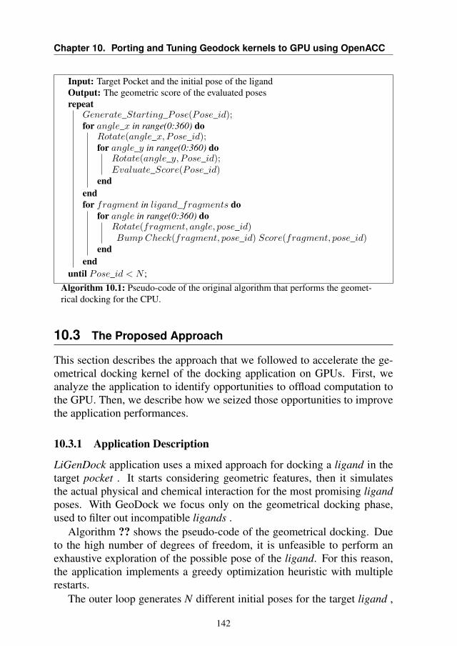
Chapter 10. Porting and Tuning Geodock kernels to GPU using OpenACC
Input: Target Pocket and the initial pose of the ligandOutput: The geometric score of the evaluated posesrepeat
Generate_Starting_Pose(Pose_id);for angle_x in range(0:360) do
Rotate(angle_x, Pose_id);for angle_y in range(0:360) do
Rotate(angle_y, Pose_id);Evaluate_Score(Pose_id)
endendfor fragment in ligand_fragments do
for angle in range(0:360) doRotate(fragment, angle, pose_id)Bump Check(fragment, pose_id) Score(fragment, pose_id)
endend
until Pose_id < N ;Algorithm 10.1: Pseudo-code of the original algorithm that performs the geomet-rical docking for the CPU.
10.3 The Proposed Approach
This section describes the approach that we followed to accelerate the ge-ometrical docking kernel of the docking application on GPUs. First, weanalyze the application to identify opportunities to offload computation tothe GPU. Then, we describe how we seized those opportunities to improvethe application performances.
10.3.1 Application Description
LiGenDock application uses a mixed approach for docking a ligand in thetarget pocket . It starts considering geometric features, then it simulatesthe actual physical and chemical interaction for the most promising ligandposes. With GeoDock we focus only on the geometrical docking phase,used to filter out incompatible ligands .
Algorithm ?? shows the pseudo-code of the geometrical docking. Dueto the high number of degrees of freedom, it is unfeasible to perform anexhaustive exploration of the possible pose of the ligand. For this reason,the application implements a greedy optimization heuristic with multiplerestarts.
The outer loop generates N different initial poses for the target ligand ,
142
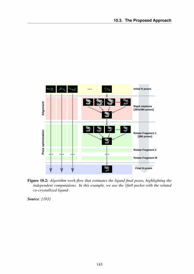
10.3. The Proposed Approach
Alig
nm
ent
Rigid rotations[360x360 poses]
Rotate Fragment 1[360 poses]
Rotate Fragment 2
Final N poses
Rotate Fragment M
Po
se o
pti
miz
atio
n
Initial N poses
Figure 10.2: Algorithm work-flow that estimates the ligand final poses, highlighting theindependent computations. In this example, we use the 1fm9 pocket with the relatedco-crystallized ligand .
Source: [193]
143
Chapter 10. Porting and Tuning Geodock kernels to GPU using OpenACC
maximizing the probability to avoid local minimum. Each iteration of theouter loop aims at docking the ith initial pose of the ligand .
Within the body of the outer loop, the docking algorithm is divided intotwo sections. The first one (lines 3-9) performs rigid rotations of the ligand, to find the best alignment with the target pocket , according to the scoringfunction. We will refer to this section of the algorithm as Rigid Rotation orAlignment. In the last section of the algorithm (lines 10-14), we optimizethe shape of the ligand by evaluating each fragment in an independent fash-ion (line 10). In particular, we rotate each fragment to find the angle thatmaximizes the scoring function without overlapping with the other atomsof the ligand (lines 11-13). We will refer to this section of the algorithmas Optimize Pose. We need to evaluate each fragment sequentially, sincea fragment may include another fragment. Therefore, if we parallelize thepose optimization over the fragments, we might change the ligand structurein an unpredictable way, invalidating the outcome of the application.
Finally, Figure 10.2 depicts the geometric docking workflow, highlight-ing data dependencies. In particular, the initial poses are independent, sinceevery initial pose represents the actual starting point of the docking algo-rithm. For every starting pose, we perform rigid rotations to select the mostsuitable alignment of the initial pose of the ligand for the target pocket .After the Rigid Rotations, we proceed with the Pose Optimization phase,evaluating each fragment of the ligand sequentially. As output, we retrieveN poses, one for each starting pose.
10.3.2 Profiling
To identify bottlenecks of the application on CPU, we profiled the applica-tion using Score-P, a well-known profiling tool [194]. Figure 10.3 reportsthe result of this analysis for the most significant functions. In particular,for each function we report the percentage of time spent in that function,comprehending children, and the number of times that it is called in thealgorithm. From the results, we noticed that the main bottleneck of theapplication is the scoring function. Even if the function itself is rather sim-ple, we need to call it every time we modify the ligand structure, to drivethe pose optimization process. In particular, the scoring function evaluates“how good” is the position of every atom of the ligand inside the pocket .The actual score of the ligand is the average score of the atoms. Due to thecode optimization, this function leverages the CPU vector units to processthe score of each atom, leading to an execution time of less than 100ns.However, due to the high number of calls from the algorithm (107), this
144
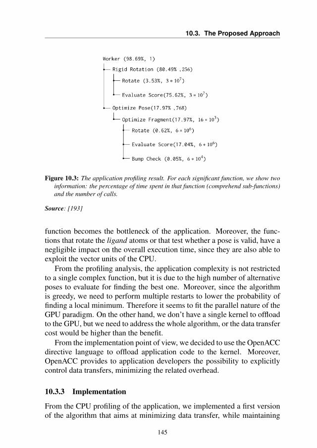
10.3. The Proposed Approach
Figure 10.3: The application profiling result. For each significant function, we show twoinformation: the percentage of time spent in that function (comprehend sub-functions)and the number of calls.
Source: [193]
function becomes the bottleneck of the application. Moreover, the func-tions that rotate the ligand atoms or that test whether a pose is valid, have anegligible impact on the overall execution time, since they are also able toexploit the vector units of the CPU.
From the profiling analysis, the application complexity is not restrictedto a single complex function, but it is due to the high number of alternativeposes to evaluate for finding the best one. Moreover, since the algorithmis greedy, we need to perform multiple restarts to lower the probability offinding a local minimum. Therefore it seems to fit the parallel nature of theGPU paradigm. On the other hand, we don’t have a single kernel to offloadto the GPU, but we need to address the whole algorithm, or the data transfercost would be higher than the benefit.
From the implementation point of view, we decided to use the OpenACCdirective language to offload application code to the kernel. Moreover,OpenACC provides to application developers the possibility to explicitlycontrol data transfers, minimizing the related overhead.
10.3.3 Implementation
From the CPU profiling of the application, we implemented a first versionof the algorithm that aims at minimizing data transfer, while maintaining
145
Chapter 10. Porting and Tuning Geodock kernels to GPU using OpenACC
the application structure. We decided to introduce parallelism on the num-ber of poses (they can all be managed in parallel and are completely inde-pendent). In this way, we transfer data only at the beginning and at the endof the docking algorithm (i.e. once in the lifetime of the ligand ).
From the implementation point of view, the following changes are re-quired to generate the binary of the offloaded kernel, i.e. the parallel regionin OpenACC jargon. All the data structures interacting with the offloadedkernel have to be compliant with the OpenACC guidelines [195] for han-dling data. In particular, this means that the data structures that interactwith the offloaded kernels must manage data transfers in the constructorand destructor. The constructor allocates memory on the device side andit copies the initialized data into device memory. The destructor must freeboth the device and the host memory. Moreover, it is mandatory to markeach function called inside the parallel region with the OpenACC “routine”directive.
Since we plan to parallelize the computation over the initial poses, we re-quire a private data structure to represent the initial pose of the ligand. TheOpenACC language provides the private keyword to express this con-cept. However, the system runtime available on our platform was not ableto support this feature1. Since it is a class containing arrays, whose copyconstructor has been redefined according to the OpenACC manual [196],it is not clear the source of the problem. Therefore, we decided to bypassthe issue by replicating the initial pose and by using manual managementof the data. Even if it required a fair amount of code refactoring, we stilltried to maintain the original structure of the application.
With this modification, we fixed the illegal access issue, but the GPUapplication was slower than the CPU one. We analyzed the problem andnoticed that this was not due to data movement since everything was resi-dent on the GPU. We found out that we were not really exploiting the par-allelism of the GPU because parallelizing the computation of all the poseswas not giving enough work to the GPU. At this point the Rigid Rotationsare still happening sequentially for every restart. Indeed, having to insist onthe same data structure for all the Rigid Rotations of one pose was limitingthe amount of exposed parallelism.
To obtain an advantage from the use of the accelerator, we had to reworkthe source code to find (and expose) more parallel computation, as shownin Algorithm 10.2. To achieve the desired result, we had to modify therotation and scoring functions, unifying them to avoid storing all the tem-
1The GeoDock execution triggered an illegal access to the GPU memory when trying to transfer the privatedata structure.
146
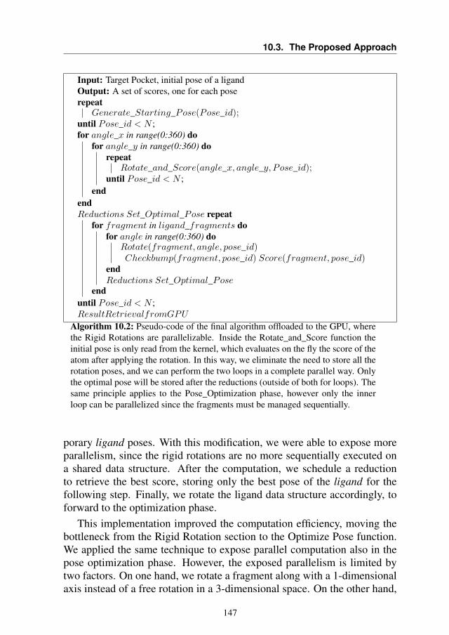
10.3. The Proposed Approach
Input: Target Pocket, initial pose of a ligandOutput: A set of scores, one for each poserepeat
Generate_Starting_Pose(Pose_id);until Pose_id < N ;for angle_x in range(0:360) do
for angle_y in range(0:360) dorepeat
Rotate_and_Score(angle_x, angle_y, Pose_id);until Pose_id < N ;
endendReductions Set_Optimal_Pose repeat
for fragment in ligand_fragments dofor angle in range(0:360) do
Rotate(fragment, angle, pose_id)Checkbump(fragment, pose_id) Score(fragment, pose_id)
endReductions Set_Optimal_Pose
enduntil Pose_id < N ;ResultRetrievalfromGPU
Algorithm 10.2: Pseudo-code of the final algorithm offloaded to the GPU, wherethe Rigid Rotations are parallelizable. Inside the Rotate_and_Score function theinitial pose is only read from the kernel, which evaluates on the fly the score of theatom after applying the rotation. In this way, we eliminate the need to store all therotation poses, and we can perform the two loops in a complete parallel way. Onlythe optimal pose will be stored after the reductions (outside of both for loops). Thesame principle applies to the Pose_Optimization phase, however only the innerloop can be parallelized since the fragments must be managed sequentially.
porary ligand poses. With this modification, we were able to expose moreparallelism, since the rigid rotations are no more sequentially executed ona shared data structure. After the computation, we schedule a reductionto retrieve the best score, storing only the best pose of the ligand for thefollowing step. Finally, we rotate the ligand data structure accordingly, toforward to the optimization phase.
This implementation improved the computation efficiency, moving thebottleneck from the Rigid Rotation section to the Optimize Pose function.We applied the same technique to expose parallel computation also in thepose optimization phase. However, the exposed parallelism is limited bytwo factors. On one hand, we rotate a fragment along with a 1-dimensionalaxis instead of a free rotation in a 3-dimensional space. On the other hand,
147
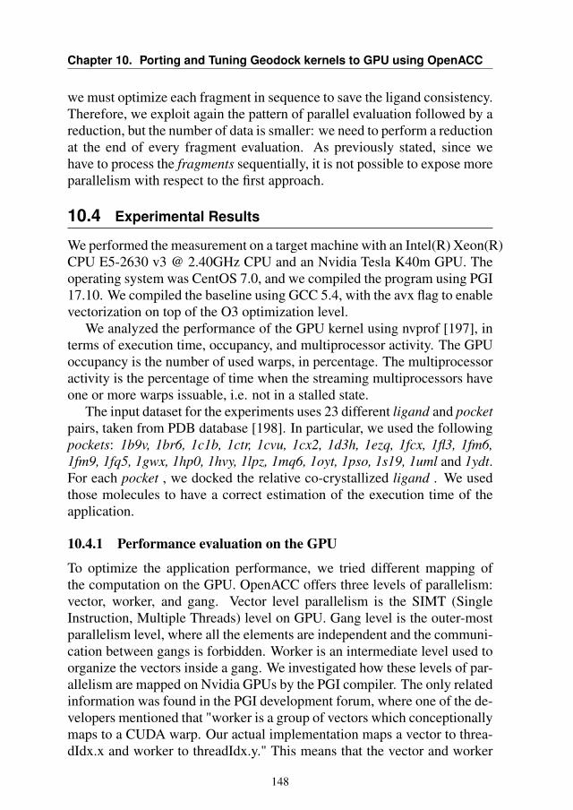
Chapter 10. Porting and Tuning Geodock kernels to GPU using OpenACC
we must optimize each fragment in sequence to save the ligand consistency.Therefore, we exploit again the pattern of parallel evaluation followed by areduction, but the number of data is smaller: we need to perform a reductionat the end of every fragment evaluation. As previously stated, since wehave to process the fragments sequentially, it is not possible to expose moreparallelism with respect to the first approach.
10.4 Experimental Results
We performed the measurement on a target machine with an Intel(R) Xeon(R)CPU E5-2630 v3 @ 2.40GHz CPU and an Nvidia Tesla K40m GPU. Theoperating system was CentOS 7.0, and we compiled the program using PGI17.10. We compiled the baseline using GCC 5.4, with the avx flag to enablevectorization on top of the O3 optimization level.
We analyzed the performance of the GPU kernel using nvprof [197], interms of execution time, occupancy, and multiprocessor activity. The GPUoccupancy is the number of used warps, in percentage. The multiprocessoractivity is the percentage of time when the streaming multiprocessors haveone or more warps issuable, i.e. not in a stalled state.
The input dataset for the experiments uses 23 different ligand and pocketpairs, taken from PDB database [198]. In particular, we used the followingpockets: 1b9v, 1br6, 1c1b, 1ctr, 1cvu, 1cx2, 1d3h, 1ezq, 1fcx, 1fl3, 1fm6,1fm9, 1fq5, 1gwx, 1hp0, 1hvy, 1lpz, 1mq6, 1oyt, 1pso, 1s19, 1uml and 1ydt.For each pocket , we docked the relative co-crystallized ligand . We usedthose molecules to have a correct estimation of the execution time of theapplication.
10.4.1 Performance evaluation on the GPU
To optimize the application performance, we tried different mapping ofthe computation on the GPU. OpenACC offers three levels of parallelism:vector, worker, and gang. Vector level parallelism is the SIMT (SingleInstruction, Multiple Threads) level on GPU. Gang level is the outer-mostparallelism level, where all the elements are independent and the communi-cation between gangs is forbidden. Worker is an intermediate level used toorganize the vectors inside a gang. We investigated how these levels of par-allelism are mapped on Nvidia GPUs by the PGI compiler. The only relatedinformation was found in the PGI development forum, where one of the de-velopers mentioned that "worker is a group of vectors which conceptionallymaps to a CUDA warp. Our actual implementation maps a vector to threa-dIdx.x and worker to threadIdx.y." This means that the vector and worker
148
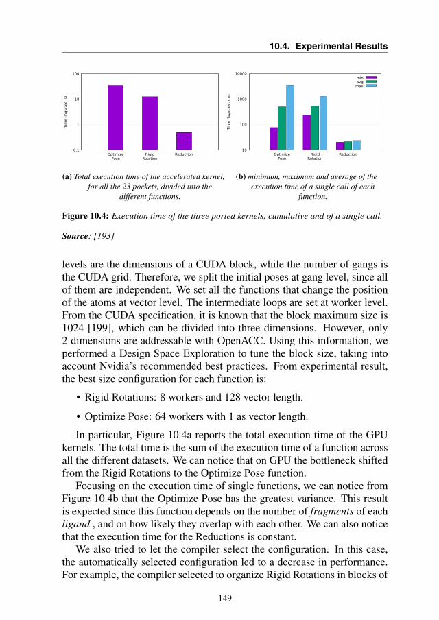
10.4. Experimental Results
0.1
1
10
100
OptimizePose
RigidRotation
Reduction
Tim
e (
log
scale
, s)
(a) Total execution time of the accelerated kernel,for all the 23 pockets, divided into the
different functions.
10
100
1000
10000
OptimizePose
RigidRotation
Reduction
Tim
e (
logsc
ale
, m
s)
minavg
max
(b) minimum, maximum and average of theexecution time of a single call of each
function.
Figure 10.4: Execution time of the three ported kernels, cumulative and of a single call.
Source: [193]
levels are the dimensions of a CUDA block, while the number of gangs isthe CUDA grid. Therefore, we split the initial poses at gang level, since allof them are independent. We set all the functions that change the positionof the atoms at vector level. The intermediate loops are set at worker level.From the CUDA specification, it is known that the block maximum size is1024 [199], which can be divided into three dimensions. However, only2 dimensions are addressable with OpenACC. Using this information, weperformed a Design Space Exploration to tune the block size, taking intoaccount Nvidia’s recommended best practices. From experimental result,the best size configuration for each function is:
• Rigid Rotations: 8 workers and 128 vector length.
• Optimize Pose: 64 workers with 1 as vector length.
In particular, Figure 10.4a reports the total execution time of the GPUkernels. The total time is the sum of the execution time of a function acrossall the different datasets. We can notice that on GPU the bottleneck shiftedfrom the Rigid Rotations to the Optimize Pose function.
Focusing on the execution time of single functions, we can notice fromFigure 10.4b that the Optimize Pose has the greatest variance. This resultis expected since this function depends on the number of fragments of eachligand , and on how likely they overlap with each other. We can also noticethat the execution time for the Reductions is constant.
We also tried to let the compiler select the configuration. In this case,the automatically selected configuration led to a decrease in performance.For example, the compiler selected to organize Rigid Rotations in blocks of
149
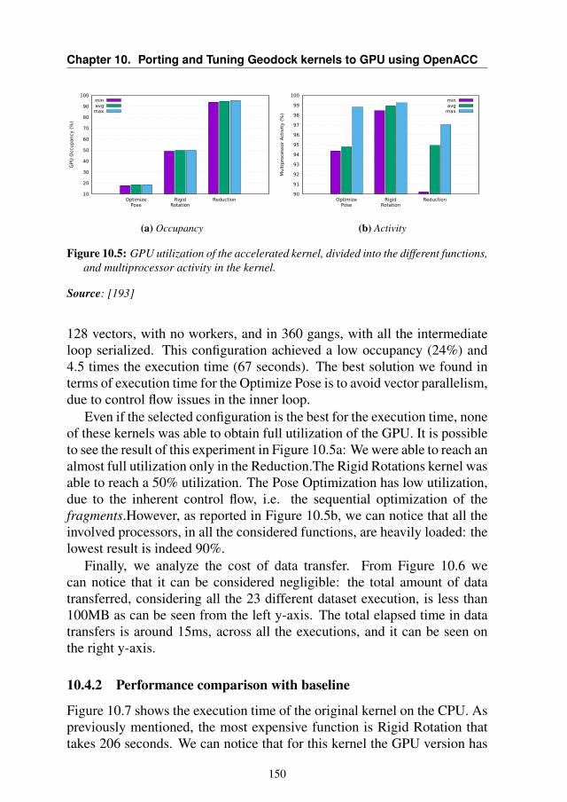
Chapter 10. Porting and Tuning Geodock kernels to GPU using OpenACC
10
20
30
40
50
60
70
80
90
100
OptimizePose
RigidRotation
Reduction
GPU
Occ
upancy
(%
)
minavg
max
(a) Occupancy
90
91
92
93
94
95
96
97
98
99
100
OptimizePose
RigidRotation
Reduction
Mult
ipro
cess
or
Act
ivit
y (
%)
minavg
max
(b) Activity
Figure 10.5: GPU utilization of the accelerated kernel, divided into the different functions,and multiprocessor activity in the kernel.
Source: [193]
128 vectors, with no workers, and in 360 gangs, with all the intermediateloop serialized. This configuration achieved a low occupancy (24%) and4.5 times the execution time (67 seconds). The best solution we found interms of execution time for the Optimize Pose is to avoid vector parallelism,due to control flow issues in the inner loop.
Even if the selected configuration is the best for the execution time, noneof these kernels was able to obtain full utilization of the GPU. It is possibleto see the result of this experiment in Figure 10.5a: We were able to reach analmost full utilization only in the Reduction.The Rigid Rotations kernel wasable to reach a 50% utilization. The Pose Optimization has low utilization,due to the inherent control flow, i.e. the sequential optimization of thefragments.However, as reported in Figure 10.5b, we can notice that all theinvolved processors, in all the considered functions, are heavily loaded: thelowest result is indeed 90%.
Finally, we analyze the cost of data transfer. From Figure 10.6 wecan notice that it can be considered negligible: the total amount of datatransferred, considering all the 23 different dataset execution, is less than100MB as can be seen from the left y-axis. The total elapsed time in datatransfers is around 15ms, across all the executions, and it can be seen onthe right y-axis.
10.4.2 Performance comparison with baseline
Figure 10.7 shows the execution time of the original kernel on the CPU. Aspreviously mentioned, the most expensive function is Rigid Rotation thattakes 206 seconds. We can notice that for this kernel the GPU version has
150
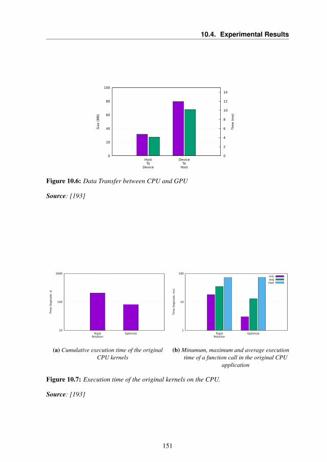
10.4. Experimental Results
0
20
40
60
80
100
HostTo
Device
DeviceTo
Host
0
2
4
6
8
10
12
14
Siz
e (
MB
)
Tim
e (
ms)
Figure 10.6: Data Transfer between CPU and GPU
Source: [193]
10
100
1000
RigidRotation
Optimize
Tim
e (
log
scale
, s)
(a) Cumulative execution time of the originalCPU kernels
1
10
100
RigidRotation
Optimize
Tim
e (
log
scale
, m
s)
minavg
max
(b) Minumum, maximum and average executiontime of a function call in the original CPU
application
Figure 10.7: Execution time of the original kernels on the CPU.
Source: [193]
151
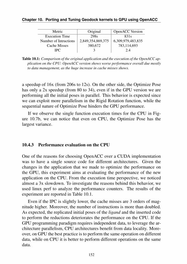
Chapter 10. Porting and Tuning Geodock kernels to GPU using OpenACC
Metric Original OpenACC VersionExecution Time 298s 831s
Number of Intructions 2,849,354,869,375 6,309,979,483,835Cache Misses 380,672 783,114,693
IPC 3 2.4
Table 10.1: Comparison of the original application and the execution of the OpenACC ap-plication on the CPU: OpenACC version shows worse performance overall due mostlyto data management, as the huge increase in cache misses shows.
a speedup of 16x (from 206s to 12s). On the other side, the Optimize Posehas only a 2x speedup (from 80 to 34), even if in the GPU version we areperforming all the initial poses in parallel. This behavior is expected sincewe can exploit more parallelism in the Rigid Rotation function, while thesequential nature of Optimize Pose hinders the GPU performance.
If we observe the single function execution times for the CPU in Fig-ure 10.7b, we can notice that even on CPU, the Optimize Pose has thelargest variance.
10.4.3 Performance evaluation on the CPU
One of the reasons for choosing OpenACC over a CUDA implementationwas to have a single source code for different architectures. Given thechanges in the application that we made to optimize the performance onthe GPU, this experiment aims at evaluating the performance of the newapplication on the CPU. From the execution time perspective, we noticedalmost a 3x slowdown. To investigate the reasons behind this behavior, weused linux perf to analyze the performance counters. The results of theexperiment are reported in Table 10.1.
Even if the IPC is slightly lower, the cache misses are 3 orders of mag-nitude higher. Moreover, the number of instructions is more than doubled.As expected, the replicated initial poses of the ligand and the inserted codeto perform the reductions deteriorates the performance on the CPU. If theGPU programming paradigm requires independent data, to leverage the ar-chitecture parallelism, CPU architectures benefit from data locality. More-over, on GPU the best practice is to perform the same operation on differentdata, while on CPU it is better to perform different operations on the samedata.
152
10.5. Summary
10.5 Summary
In the drug discovery process, the virtual screening of a large chemicallibrary is a crucial task. The benefits of an improvement in the time spent onevaluating the interaction from a ligand and the target pocket , are twofold.On one side it reduces the monetary cost of the process, on the other sideit enables the end-user to increase the number of the evaluated ligands ,increasing the probability of finding a better solution.
In this chapter, we focued on a newer version of GeoDock, again op-timized only for the CPU, and we performed a porting of the most com-pute intensive kernel to the GPU using the OpenACC directive language.We performed an experimental campaign to evaluate the performance ofthe application in terms of execution time, occupancy, and multiprocessoractivity. We also evaluated the OpenACC paradigm as "write once run ev-erywhere", and noticed that the application has to be changed to obtainperformances on different architectures.
We believe that it is possible to further improve the obtained resultswith a different approach. In the following chapter, we reorganized theapplication structure to exploit asynchronous queues and offload only thesections with heavy parallelism (i.e. the Rigid Rotation kernel), while usingthe CPU for the control flow bound sections (i.e. the Optimize Pose kernel).
The outcome of this work has been published in the 6th internationalworkshop on Parallelism in Bioinformatics 2018 [193].
153

CHAPTER11Optimizing GeoDock Throughput in
Heterogeneous Platforms
In this chapter, we further optimize the geometric docking application totake full advantage of the whole heterogeneous platform. In particular, inthe previous chapter, we have seen that simply porting the kernel to theGPU gives an improvement in performances, however, it has drawbacks.The most obvious one is that it leaves the CPU idle. Moreover, even if weconsider using the CPU to run the same kernels in parallel, distributing thedataset between the two compute units, we noticed that different sectionsof the application are more suitable for the different architectures.
With this chapter we investigate a different way to divide the compu-tation across the available computing resources, trying to bind the compu-tation to the most suitable architecture. From the implementation point ofview, we used OpenMP on top of the OpenACC implementation to organizethe computation.
We show with an experimental campaign that this approach is able tofully exploit the underlying node and obtain a better throughput up to 25%just with a re-organization of the computation without changing the com-putational resources available on the node.
155
Chapter 11. Optimizing GeoDock Throughput in Heterogeneous Platforms
11.1 Introduction
As we already mentioned, power consumption is becoming a key factor inthe HPC context. For this reason, accelerators have begun to be used along-side the traditional CPUs in this context. Among them, the most commonlyused accelerators are GPGPUs. Indeed, most of the top positions in boththe Top500 and Green500 are occupied by heterogeneous platforms thatexploit the GPGPU as an accelerator. Depending on the application al-gorithm, hardware accelerators might significantly improve the applicationthroughput with respect to general purposes CPUs, considering the samepower consumption.
However, to create a heterogeneous application the programmer mustconsider the characteristics of the application and of the available computeunits. In the previous chapter (Chapter 10) we investigated the benefits andlimitations of using the OpenACC [192] language extension in a molec-ular docking application, to accelerate the computation done in the mostcompute-intensive kernels of GeoDock. In this chapter, we implement ahybrid version by using OpenMP [200] and OpenACC to leverage opti-mally all the processing elements on a heterogeneous node. In particular,given the limitation analyzed in the previous chapter, we aim at mappingeach phase of the application on the most suitable processing element. Tosummarize, the contributions of this chapter are the following:
• We propose a Hybrid CPU/GPU version of the geometric docking al-gorithm capable to fully exploit the node heterogeneity;
• We analyze the resource utilization of the different solutions to findthe best configuration also in presence of multi-GPU nodes, searchingfor the best balance.
• We discuss the obtained results, comparing them with the sequentialCPU application, the GPU implementation of the previous chapter andthe traditional data-splitting across the different compute units of thedataset
In the context of the global framework, this chapter is focused on opti-mizing heterogeneity in the application, and not on the self-tuning at run-time. Indeed, as we can notice in Figure 11.1, the involved components arethe same as the previous chapter: the enriched code with the GPU kernel,without any runtime autotuning functionality inserted in. Nonetheless, thiswork is still in the context of the global framework, because it is focused ontuning the application. The performed tuning in this case is not automatical
156
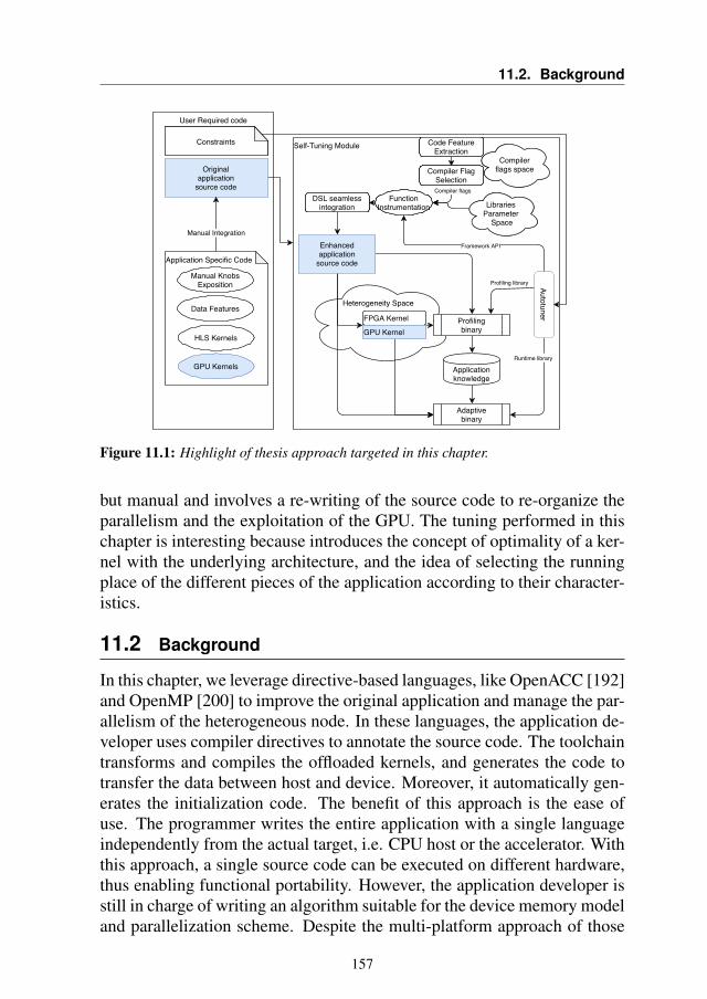
11.2. Background
User Required code
Self-Tuning Module
Heterogeneity Space
Originalapplication
source code
Code FeatureExtraction
Compilerflags space
Compiler flags
Compiler FlagSelection
Libraries Parameter
Space
DSL seamlessintegration
Enhancedapplication
source code
Profilingbinary
Applicationknowledge
Adaptivebinary
Runtime library
Framework API
Autotuner
Profiling library
Manual Integration
Application Specific Code
Data Features
HLS Kernels
GPU Kernels
FPGA Kernel
GPU Kernel
Constraints
Manual KnobsExposition
FunctionInstrumentation
Constraints Code FeatureExtraction
Compiler FlagSelection
FunctionInstrumentation Libraries
Parameter Space
Compilerflags space
DSL seamlessintegration
Autotuner
Figure 11.1: Highlight of thesis approach targeted in this chapter.
but manual and involves a re-writing of the source code to re-organize theparallelism and the exploitation of the GPU. The tuning performed in thischapter is interesting because introduces the concept of optimality of a ker-nel with the underlying architecture, and the idea of selecting the runningplace of the different pieces of the application according to their character-istics.
11.2 Background
In this chapter, we leverage directive-based languages, like OpenACC [192]and OpenMP [200] to improve the original application and manage the par-allelism of the heterogeneous node. In these languages, the application de-veloper uses compiler directives to annotate the source code. The toolchaintransforms and compiles the offloaded kernels, and generates the code totransfer the data between host and device. Moreover, it automatically gen-erates the initialization code. The benefit of this approach is the ease ofuse. The programmer writes the entire application with a single languageindependently from the actual target, i.e. CPU host or the accelerator. Withthis approach, a single source code can be executed on different hardware,thus enabling functional portability. However, the application developer isstill in charge of writing an algorithm suitable for the device memory modeland parallelization scheme. Despite the multi-platform approach of those
157
Chapter 11. Optimizing GeoDock Throughput in Heterogeneous Platforms
languages, the kernels must be tuned according to the target platform, sinceperformance portability is still an open problem [201]. Indeed, one of theconclusions of the previous chapter is that the code modified and optimizedfor the GPU was not efficient when compiled and run on the CPU as theoriginal code.
To improve computation efficiency, we aim at optimizing the exploita-tion of all the computational resources available in an HPC node, whilecontinuing to use MPI for inter-node communication. In modern systems,the HPC node typically includes several CPUs and GPUs. The multi-GPUproblem has been investigated in literature. For example, the approachesproposed in [202, 203] suggest extending OpenMP to support multiple ac-celerators seamlessly. OpenACC has runtime functions to support the uti-lization of multiple GPU, however, lacks GPU to GPU data transfer, insingle node [204] and multinode [205]. A previous work in literature [206]investigates a hybrid approach with OpenMP and OpenACC. It proposesthe usage of OpenMP to support a multi-GPU OpenACC application, as-signing each GPU to an OpenMP thread. In this context, each OpenMPthread performs the data transfer between the host and the target device,without performing any other computation.
In this chapter, we extend the previous one by suggesting a new ap-proach that offloads to the GPU the most compute-intensive kernels, us-ing a hybrid approach of OpenMP and OpenACC. In this way, we exploitmulti-GPU nodes offloading to accelerators only the kernels that maximizethe advantage of being run on the GPU, while keeping the utilization of thisresource as high as possible. Unlikely previous approaches, we rely on theCPU to execute the kernels that are less suitable for the GPU. Moreover,to maximize the utilization of the resources, every OpenMP thread has aGPU associated. In this way, the computing thread has access to both theCPU and the GPU. Thanks to this, we can split the workload across thecompute units, associating the kernels to the compute units according tothe characteristics of the function to evaluate and of the compute unit itself.
11.3 The Proposed Approach
In this section, we describe the proposed approach to accelerate GeoDockusing GPUs. First, we quickly recap in Section 11.3.1 the work done inthe previous chapter where we accelerated the whole algorithm with GPUs,relying on OpenACC. Then, we describe in Section 11.3.2 the analysis thatleads us to implement the hybrid OpenMP/OpenACC solution. As we havealready explained, the idea is to allocate the workload on the heterogeneous
158
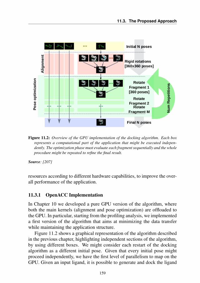
11.3. The Proposed Approach
Figure 11.2: Overview of the GPU implementation of the docking algorithm. Each boxrepresents a computational part of the application that might be executed indepen-dently. The optimization phase must evaluate each fragment sequentially and the wholeprocedure might be repeated to refine the final result.
Source: [207]
resources according to different hardware capabilities, to improve the over-all performance of the application.
11.3.1 OpenACC Implementation
In Chapter 10 we developed a pure GPU version of the algorithm, whereboth the main kernels (alignment and pose optimization) are offloaded tothe GPU. In particular, starting from the profiling analysis, we implementeda first version of the algorithm that aims at minimizing the data transferwhile maintaining the application structure.
Figure 11.2 shows a graphical representation of the algorithm describedin the previous chapter, highlighting independent sections of the algorithm,by using different boxes. We might consider each restart of the dockingalgorithm as a different initial pose. Given that every initial pose mightproceed independently, we have the first level of parallelism to map on theGPU. Given an input ligand, it is possible to generate and dock the ligand
159
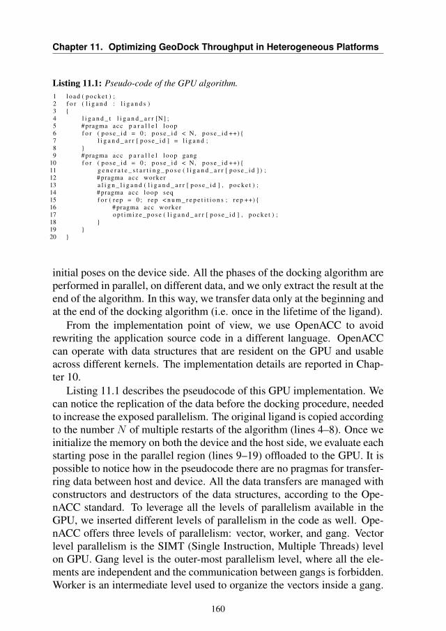
Chapter 11. Optimizing GeoDock Throughput in Heterogeneous Platforms
Listing 11.1: Pseudo-code of the GPU algorithm.1 l o a d ( p o c k e t ) ;2 f o r ( l i g a n d : l i g a n d s )3 {4 l i g a n d _ t l i g a n d _ a r r [N ] ;5 # pragma acc p a r a l l e l l oop6 f o r ( p o s e _ i d = 0 ; p o s e _ i d < N, p o s e _ i d ++) {7 l i g a n d _ a r r [ p o s e _ i d ] = l i g a n d ;8 }9 # pragma acc p a r a l l e l l oop gang
10 f o r ( p o s e _ i d = 0 ; p o s e _ i d < N, p o s e _ i d ++) {11 g e n e r a t e _ s t a r t i n g _ p o s e ( l i g a n d _ a r r [ p o s e _ i d ] ) ;12 # pragma acc worker13 a l i g n _ l i g a n d ( l i g a n d _ a r r [ p o s e _ i d ] , p o c k e t ) ;14 # pragma acc loop seq15 f o r ( r e p = 0 ; r e p < n u m _ r e p e t i t i o n s ; r e p ++) {16 # pragma acc worker17 o p t i m i z e _ p o s e ( l i g a n d _ a r r [ p o s e _ i d ] , p o c k e t ) ;18 }19 }20 }
initial poses on the device side. All the phases of the docking algorithm areperformed in parallel, on different data, and we only extract the result at theend of the algorithm. In this way, we transfer data only at the beginning andat the end of the docking algorithm (i.e. once in the lifetime of the ligand).
From the implementation point of view, we use OpenACC to avoidrewriting the application source code in a different language. OpenACCcan operate with data structures that are resident on the GPU and usableacross different kernels. The implementation details are reported in Chap-ter 10.
Listing 11.1 describes the pseudocode of this GPU implementation. Wecan notice the replication of the data before the docking procedure, neededto increase the exposed parallelism. The original ligand is copied accordingto the number N of multiple restarts of the algorithm (lines 4–8). Once weinitialize the memory on both the device and the host side, we evaluate eachstarting pose in the parallel region (lines 9–19) offloaded to the GPU. It ispossible to notice how in the pseudocode there are no pragmas for transfer-ring data between host and device. All the data transfers are managed withconstructors and destructors of the data structures, according to the Ope-nACC standard. To leverage all the levels of parallelism available in theGPU, we inserted different levels of parallelism in the code as well. Ope-nACC offers three levels of parallelism: vector, worker, and gang. Vectorlevel parallelism is the SIMT (Single Instruction, Multiple Threads) levelon GPU. Gang level is the outer-most parallelism level, where all the ele-ments are independent and the communication between gangs is forbidden.Worker is an intermediate level used to organize the vectors inside a gang.
160
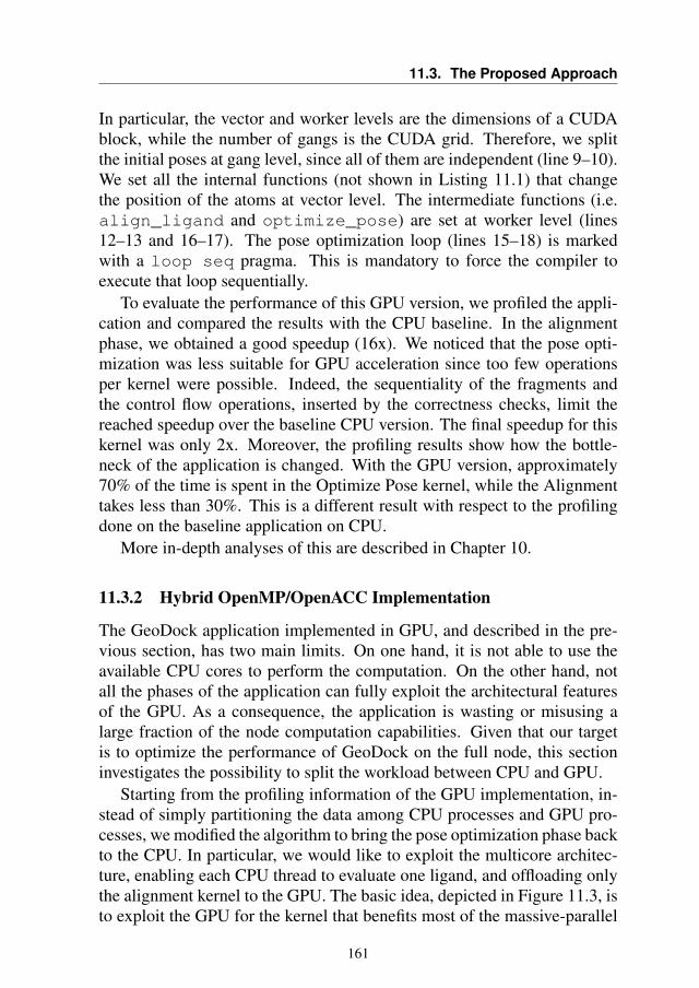
11.3. The Proposed Approach
In particular, the vector and worker levels are the dimensions of a CUDAblock, while the number of gangs is the CUDA grid. Therefore, we splitthe initial poses at gang level, since all of them are independent (line 9–10).We set all the internal functions (not shown in Listing 11.1) that changethe position of the atoms at vector level. The intermediate functions (i.e.align_ligand and optimize_pose) are set at worker level (lines12–13 and 16–17). The pose optimization loop (lines 15–18) is markedwith a loop seq pragma. This is mandatory to force the compiler toexecute that loop sequentially.
To evaluate the performance of this GPU version, we profiled the appli-cation and compared the results with the CPU baseline. In the alignmentphase, we obtained a good speedup (16x). We noticed that the pose opti-mization was less suitable for GPU acceleration since too few operationsper kernel were possible. Indeed, the sequentiality of the fragments andthe control flow operations, inserted by the correctness checks, limit thereached speedup over the baseline CPU version. The final speedup for thiskernel was only 2x. Moreover, the profiling results show how the bottle-neck of the application is changed. With the GPU version, approximately70% of the time is spent in the Optimize Pose kernel, while the Alignmenttakes less than 30%. This is a different result with respect to the profilingdone on the baseline application on CPU.
More in-depth analyses of this are described in Chapter 10.
11.3.2 Hybrid OpenMP/OpenACC Implementation
The GeoDock application implemented in GPU, and described in the pre-vious section, has two main limits. On one hand, it is not able to use theavailable CPU cores to perform the computation. On the other hand, notall the phases of the application can fully exploit the architectural featuresof the GPU. As a consequence, the application is wasting or misusing alarge fraction of the node computation capabilities. Given that our targetis to optimize the performance of GeoDock on the full node, this sectioninvestigates the possibility to split the workload between CPU and GPU.
Starting from the profiling information of the GPU implementation, in-stead of simply partitioning the data among CPU processes and GPU pro-cesses, we modified the algorithm to bring the pose optimization phase backto the CPU. In particular, we would like to exploit the multicore architec-ture, enabling each CPU thread to evaluate one ligand, and offloading onlythe alignment kernel to the GPU. The basic idea, depicted in Figure 11.3, isto exploit the GPU for the kernel that benefits most of the massive-parallel
161
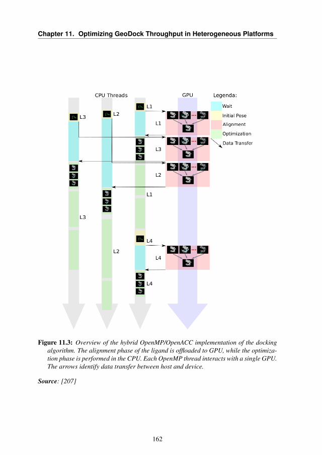
Chapter 11. Optimizing GeoDock Throughput in Heterogeneous Platforms
Figure 11.3: Overview of the hybrid OpenMP/OpenACC implementation of the dockingalgorithm. The alignment phase of the ligand is offloaded to GPU, while the optimiza-tion phase is performed in the CPU. Each OpenMP thread interacts with a single GPU.The arrows identify data transfer between host and device.
Source: [207]
162
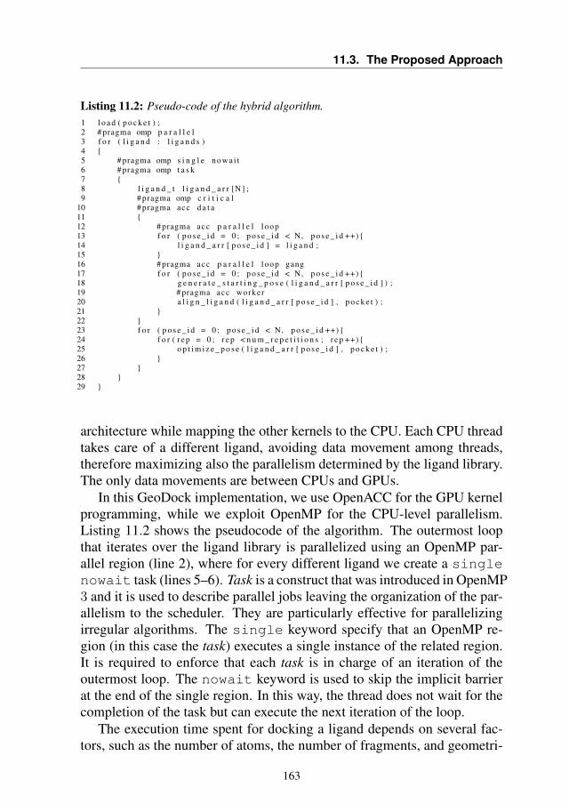
11.3. The Proposed Approach
Listing 11.2: Pseudo-code of the hybrid algorithm.1 l o a d ( p o c k e t ) ;2 # pragma omp p a r a l l e l3 f o r ( l i g a n d : l i g a n d s )4 {5 # pragma omp s i n g l e n ow a i t6 # pragma omp t a s k7 {8 l i g a n d _ t l i g a n d _ a r r [N ] ;9 # pragma omp c r i t i c a l
10 # pragma acc d a t a11 {12 # pragma acc p a r a l l e l l oop13 f o r ( p o s e _ i d = 0 ; p o s e _ i d < N, p o s e _ i d ++) {14 l i g a n d _ a r r [ p o s e _ i d ] = l i g a n d ;15 }16 # pragma acc p a r a l l e l l oop gang17 f o r ( p o s e _ i d = 0 ; p o s e _ i d < N, p o s e _ i d ++) {18 g e n e r a t e _ s t a r t i n g _ p o s e ( l i g a n d _ a r r [ p o s e _ i d ] ) ;19 # pragma acc worker20 a l i g n _ l i g a n d ( l i g a n d _ a r r [ p o s e _ i d ] , p o c k e t ) ;21 }22 }23 f o r ( p o s e _ i d = 0 ; p o s e _ i d < N, p o s e _ i d ++) {24 f o r ( r e p = 0 ; r e p < n u m _ r e p e t i t i o n s ; r e p ++) {25 o p t i m i z e _ p o s e ( l i g a n d _ a r r [ p o s e _ i d ] , p o c k e t ) ;26 }27 }28 }29 }
architecture while mapping the other kernels to the CPU. Each CPU threadtakes care of a different ligand, avoiding data movement among threads,therefore maximizing also the parallelism determined by the ligand library.The only data movements are between CPUs and GPUs.
In this GeoDock implementation, we use OpenACC for the GPU kernelprogramming, while we exploit OpenMP for the CPU-level parallelism.Listing 11.2 shows the pseudocode of the algorithm. The outermost loopthat iterates over the ligand library is parallelized using an OpenMP par-allel region (line 2), where for every different ligand we create a singlenowait task (lines 5–6). Task is a construct that was introduced in OpenMP3 and it is used to describe parallel jobs leaving the organization of the par-allelism to the scheduler. They are particularly effective for parallelizingirregular algorithms. The single keyword specify that an OpenMP re-gion (in this case the task) executes a single instance of the related region.It is required to enforce that each task is in charge of an iteration of theoutermost loop. The nowait keyword is used to skip the implicit barrierat the end of the single region. In this way, the thread does not wait for thecompletion of the task but can execute the next iteration of the loop.
The execution time spent for docking a ligand depends on several fac-tors, such as the number of atoms, the number of fragments, and geometri-
163
Chapter 11. Optimizing GeoDock Throughput in Heterogeneous Platforms
cal properties of both the target pocket and ligand. Since these factors mightdrastically change between ligands of the same library, we might considerour docking algorithm as an irregular application. Therefore, the proposedimplementation leverages the tasks construct to create a task for every lig-and to be docked. As soon as an OpenMP thread becomes free, a pendingtask is assigned to it, until there is a task waiting to be executed. Moreover,we use the tied task implementation to limit migration, restraining a task tobe executed on the same thread that generated it. Moreover, we bind eachOpenMP thread to a physical core, by using the OpenMP environment vari-able OMP_PLACES=cores. In this way, we can associate a ligand to onephysical core, avoiding the extra movement of the data.
Beside the Task construct, we tried to exploit other OpenMP strategiesto make the application parallel. In particular, we evaluated the taskloopkeyword, which is a construct used to create one task for each iteration ofa loop, and the traditional parallel for. The first construct is not supportedby PGI 17.10, so we were not able to exploit it. The parallel for has em-pirically shown slightly worse throughput in the considered case. We alsotried all the OpenMP scheduling algorithms (static, dynamic, and guided)and none of them was able to improve the performance obtained with thetask construct.
The GPU kernel is implemented inside an OpenMP critical region(line 9) to avoid race conditions. We also considered using OpenACC fea-tures, such as asynchronous queues, however, they performed worse thanthis implementation. We exploit the implicit barrier at the end of the par-allel region to enforce thread synchronization at the end of the library ofligands to be docked.
The GeoDock algorithm implementation is similar to the one describedin Section 11.3.1. In particular, the data replication (lines 12–15) and thealignment phase (lines 16–21) are almost the same. The only difference isin the data structure implementation, due to the limited support of C++ stan-dard libraries from OpenACC. For this reason, we manually managed datacopies before and after the critical section used to offload the alignment tothe GPU. These changes are omitted in the application pseudocode. How-ever, we encountered a key issue in the memory management of the hybridsolution. In the GPU version, we used CUDA unified memory to reducethe impact of data organization on the application developer. This featureenables addresses accessible from different types of architectures (normalCPU and CUDA GPU cores) hiding the complexity of the managementfrom the programmer. If we use this implementation, the Unified Memory
164
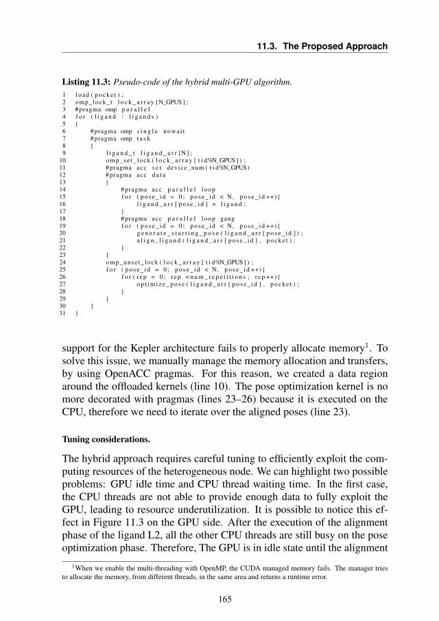
11.3. The Proposed Approach
Listing 11.3: Pseudo-code of the hybrid multi-GPU algorithm.1 l o a d ( p o c k e t ) ;2 omp_lock_t l o c k _ a r r a y [N_GPUS ] ;3 # pragma omp p a r a l l e l4 f o r ( l i g a n d : l i g a n d s )5 {6 # pragma omp s i n g l e n ow a i t7 # pragma omp t a s k8 {9 l i g a n d _ t l i g a n d _ a r r [N ] ;
10 omp_se t_ lock ( l o c k _ a r r a y [ t i d%N_GPUS ] ) ;11 # pragma acc s e t device_num ( t i d%N_GPUS)12 # pragma acc d a t a13 {14 # pragma acc p a r a l l e l l oop15 f o r ( p o s e _ i d = 0 ; p o s e _ i d < N, p o s e _ i d ++) {16 l i g a n d _ a r r [ p o s e _ i d ] = l i g a n d ;17 }18 # pragma acc p a r a l l e l l oop gang19 f o r ( p o s e _ i d = 0 ; p o s e _ i d < N, p o s e _ i d ++) {20 g e n e r a t e _ s t a r t i n g _ p o s e ( l i g a n d _ a r r [ p o s e _ i d ] ) ;21 a l i g n _ l i g a n d ( l i g a n d _ a r r [ p o s e _ i d ] , p o c k e t ) ;22 }23 }24 omp_unse t_ lock ( l o c k _ a r r a y [ t i d%N_GPUS ] ) ;25 f o r ( p o s e _ i d = 0 ; p o s e _ i d < N, p o s e _ i d ++) {26 f o r ( r e p = 0 ; r e p < n u m _ r e p e t i t i o n s ; r e p ++) {27 o p t i m i z e _ p o s e ( l i g a n d _ a r r [ p o s e _ i d ] , p o c k e t ) ;28 }29 }30 }31 }
support for the Kepler architecture fails to properly allocate memory1. Tosolve this issue, we manually manage the memory allocation and transfers,by using OpenACC pragmas. For this reason, we created a data regionaround the offloaded kernels (line 10). The pose optimization kernel is nomore decorated with pragmas (lines 23–26) because it is executed on theCPU, therefore we need to iterate over the aligned poses (line 23).
Tuning considerations.
The hybrid approach requires careful tuning to efficiently exploit the com-puting resources of the heterogeneous node. We can highlight two possibleproblems: GPU idle time and CPU thread waiting time. In the first case,the CPU threads are not able to provide enough data to fully exploit theGPU, leading to resource underutilization. It is possible to notice this ef-fect in Figure 11.3 on the GPU side. After the execution of the alignmentphase of the ligand L2, all the other CPU threads are still busy on the poseoptimization phase. Therefore, The GPU is in idle state until the alignment
1When we enable the multi-threading with OpenMP, the CUDA managed memory fails. The manager triesto allocate the memory, from different threads, in the same area and returns a runtime error.
165
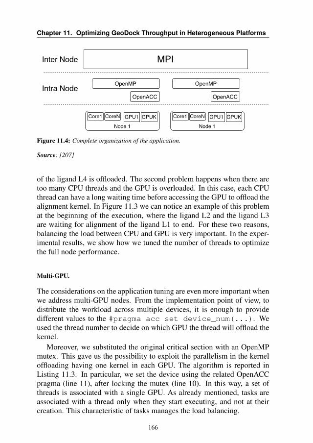
Chapter 11. Optimizing GeoDock Throughput in Heterogeneous Platforms
MPI
Node 1
Inter Node
Intra Node OpenMP
OpenACC
Core1
OpenMP
OpenACC
CoreN GPU1 GPUK
Node 1
Core1 CoreN GPU1 GPUK
Figure 11.4: Complete organization of the application.
Source: [207]
of the ligand L4 is offloaded. The second problem happens when there aretoo many CPU threads and the GPU is overloaded. In this case, each CPUthread can have a long waiting time before accessing the GPU to offload thealignment kernel. In Figure 11.3 we can notice an example of this problemat the beginning of the execution, where the ligand L2 and the ligand L3are waiting for alignment of the ligand L1 to end. For these two reasons,balancing the load between CPU and GPU is very important. In the exper-imental results, we show how we tuned the number of threads to optimizethe full node performance.
Multi-GPU.
The considerations on the application tuning are even more important whenwe address multi-GPU nodes. From the implementation point of view, todistribute the workload across multiple devices, it is enough to providedifferent values to the #pragma acc set device_num(...). Weused the thread number to decide on which GPU the thread will offload thekernel.
Moreover, we substituted the original critical section with an OpenMPmutex. This gave us the possibility to exploit the parallelism in the kerneloffloading having one kernel in each GPU. The algorithm is reported inListing 11.3. In particular, we set the device using the related OpenACCpragma (line 11), after locking the mutex (line 10). In this way, a set ofthreads is associated with a single GPU. As already mentioned, tasks areassociated with a thread only when they start executing, and not at theircreation. This characteristic of tasks manages the load balancing.
166
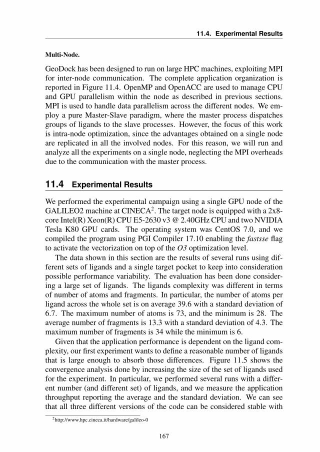
11.4. Experimental Results
Multi-Node.
GeoDock has been designed to run on large HPC machines, exploiting MPIfor inter-node communication. The complete application organization isreported in Figure 11.4. OpenMP and OpenACC are used to manage CPUand GPU parallelism within the node as described in previous sections.MPI is used to handle data parallelism across the different nodes. We em-ploy a pure Master-Slave paradigm, where the master process dispatchesgroups of ligands to the slave processes. However, the focus of this workis intra-node optimization, since the advantages obtained on a single nodeare replicated in all the involved nodes. For this reason, we will run andanalyze all the experiments on a single node, neglecting the MPI overheadsdue to the communication with the master process.
11.4 Experimental Results
We performed the experimental campaign using a single GPU node of theGALILEO2 machine at CINECA2. The target node is equipped with a 2x8-core Intel(R) Xeon(R) CPU E5-2630 v3 @ 2.40GHz CPU and two NVIDIATesla K80 GPU cards. The operating system was CentOS 7.0, and wecompiled the program using PGI Compiler 17.10 enabling the fastsse flagto activate the vectorization on top of the O3 optimization level.
The data shown in this section are the results of several runs using dif-ferent sets of ligands and a single target pocket to keep into considerationpossible performance variability. The evaluation has been done consider-ing a large set of ligands. The ligands complexity was different in termsof number of atoms and fragments. In particular, the number of atoms perligand across the whole set is on average 39.6 with a standard deviation of6.7. The maximum number of atoms is 73, and the minimum is 28. Theaverage number of fragments is 13.3 with a standard deviation of 4.3. Themaximum number of fragments is 34 while the minimum is 6.
Given that the application performance is dependent on the ligand com-plexity, our first experiment wants to define a reasonable number of ligandsthat is large enough to absorb those differences. Figure 11.5 shows theconvergence analysis done by increasing the size of the set of ligands usedfor the experiment. In particular, we performed several runs with a differ-ent number (and different set) of ligands, and we measure the applicationthroughput reporting the average and the standard deviation. We can seethat all three different versions of the code can be considered stable with
2http://www.hpc.cineca.it/hardware/galileo-0
167
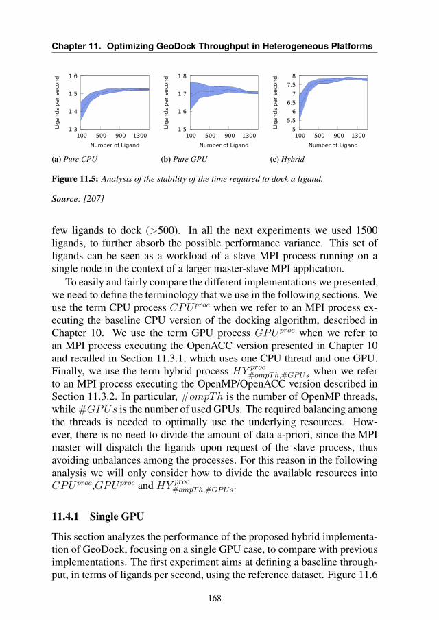
Chapter 11. Optimizing GeoDock Throughput in Heterogeneous Platforms
1.3
1.4
1.5
1.6
100 500 900 1300
Lig
and
s p
er
seco
nd
Number of Ligand
(a) Pure CPU
1.5
1.6
1.7
1.8
100 500 900 1300
Lig
and
s p
er
seco
nd
Number of Ligand
(b) Pure GPU
5
5.5
6
6.5
7
7.5
8
100 500 900 1300
Lig
and
s p
er
seco
nd
Number of Ligand
(c) Hybrid
Figure 11.5: Analysis of the stability of the time required to dock a ligand.
Source: [207]
few ligands to dock (>500). In all the next experiments we used 1500ligands, to further absorb the possible performance variance. This set ofligands can be seen as a workload of a slave MPI process running on asingle node in the context of a larger master-slave MPI application.
To easily and fairly compare the different implementations we presented,we need to define the terminology that we use in the following sections. Weuse the term CPU process CPUproc when we refer to an MPI process ex-ecuting the baseline CPU version of the docking algorithm, described inChapter 10. We use the term GPU process GPUproc when we refer toan MPI process executing the OpenACC version presented in Chapter 10and recalled in Section 11.3.1, which uses one CPU thread and one GPU.Finally, we use the term hybrid process HY proc
#ompTh,#GPUs when we referto an MPI process executing the OpenMP/OpenACC version described inSection 11.3.2. In particular, #ompTh is the number of OpenMP threads,while #GPUs is the number of used GPUs. The required balancing amongthe threads is needed to optimally use the underlying resources. How-ever, there is no need to divide the amount of data a-priori, since the MPImaster will dispatch the ligands upon request of the slave process, thusavoiding unbalances among the processes. For this reason in the followinganalysis we will only consider how to divide the available resources intoCPUproc,GPUproc and HY proc
#ompTh,#GPUs.
11.4.1 Single GPU
This section analyzes the performance of the proposed hybrid implementa-tion of GeoDock, focusing on a single GPU case, to compare with previousimplementations. The first experiment aims at defining a baseline through-put, in terms of ligands per second, using the reference dataset. Figure 11.6
168
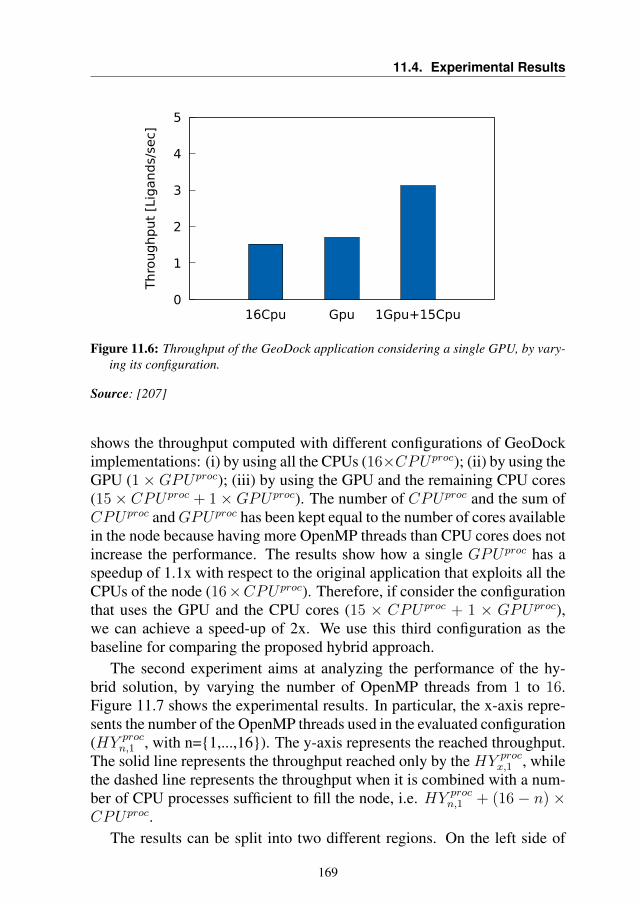
11.4. Experimental Results
0
1
2
3
4
5
16Cpu Gpu 1Gpu+15Cpu
Thro
ughput
[Lig
ands/
sec]
Figure 11.6: Throughput of the GeoDock application considering a single GPU, by vary-ing its configuration.
Source: [207]
shows the throughput computed with different configurations of GeoDockimplementations: (i) by using all the CPUs (16×CPUproc); (ii) by using theGPU (1×GPUproc); (iii) by using the GPU and the remaining CPU cores(15× CPUproc + 1×GPUproc). The number of CPUproc and the sum ofCPUproc andGPUproc has been kept equal to the number of cores availablein the node because having more OpenMP threads than CPU cores does notincrease the performance. The results show how a single GPUproc has aspeedup of 1.1x with respect to the original application that exploits all theCPUs of the node (16×CPUproc). Therefore, if consider the configurationthat uses the GPU and the CPU cores (15 × CPUproc + 1 × GPUproc),we can achieve a speed-up of 2x. We use this third configuration as thebaseline for comparing the proposed hybrid approach.
The second experiment aims at analyzing the performance of the hy-brid solution, by varying the number of OpenMP threads from 1 to 16.Figure 11.7 shows the experimental results. In particular, the x-axis repre-sents the number of the OpenMP threads used in the evaluated configuration(HY proc
n,1 , with n={1,...,16}). The y-axis represents the reached throughput.The solid line represents the throughput reached only by the HY proc
x,1 , whilethe dashed line represents the throughput when it is combined with a num-ber of CPU processes sufficient to fill the node, i.e. HY proc
n,1 + (16 − n) ×CPUproc.
The results can be split into two different regions. On the left side of
169
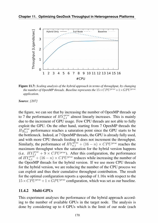
Chapter 11. Optimizing GeoDock Throughput in Heterogeneous Platforms
0
1
2
3
4
1 2 3 4 5 6 7 8 9 10 11 12 13 14 15 16
Thro
ughput
[Lig
ands/
sec]
#CPU
Hybrid Only Full Node Baseline
Figure 11.7: Scaling analysis of the hybrid approach in terms of throughput, by changingthe number of OpenMP threads. Baseline represents the 15×CPUproc+1×GPUproc
application.
Source: [207]
the figure, we can see that by increasing the number of OpenMP threads upto 7 the performance of HY proc
n,1 almost linearly increases. This is mainlydue to the increment of GPU usage. Few CPU threads are not able to fullyexploit the GPU. On the other hand, starting from 7 OpenMP threads theHyprocn,1 performance reaches a saturation point since the GPU starts to bethe bottleneck. Indeed, at 7 OpenMP threads, the GPU is already fully used,and with more CPU threads feeding it does not increment the throughput.Similarly, the performance of HY proc
n,1 + (16 − n) × CPUproc reaches themaximum throughput when the saturation for the hybrid version happens(i.e. HY proc
7,1 + 9 × CPUproc). After this configuration, the performanceof HY proc
n,1 + (16− n)× CPUproc reduces while increasing the number ofthe OpenMP threads for the hybrid version. If we use more CPU threadsfor the hybrid version, we are reducing the number of the CPU process wecan exploit and thus their cumulative throughput contribution. The resultfor the optimal configuration reports a speedup of 1.16x with respect to the15×CPUproc+1×GPUproc configuration, which was set as our baseline.
11.4.2 Multi-GPUs
This experiment analyses the performance of the hybrid approach accord-ing to the number of available GPUs in the target node. The analysis isdone by considering up to 4 GPUs which is the limit of our node (each
170
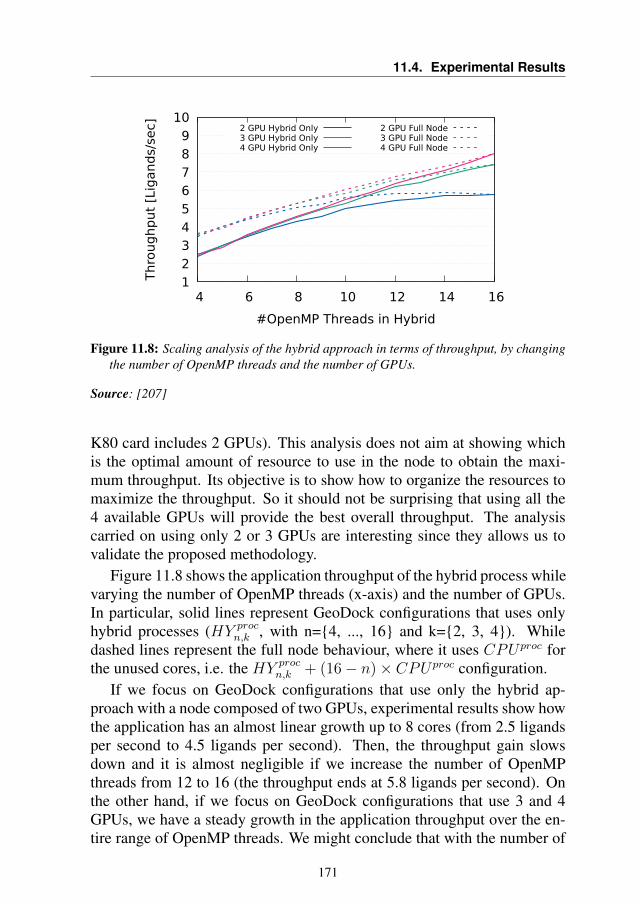
11.4. Experimental Results
1 2 3 4 5 6 7 8 9
10
4 6 8 10 12 14 16
Thro
ughput
[Lig
ands/
sec]
#OpenMP Threads in Hybrid
2 GPU Hybrid Only3 GPU Hybrid Only4 GPU Hybrid Only
2 GPU Full Node3 GPU Full Node4 GPU Full Node
Figure 11.8: Scaling analysis of the hybrid approach in terms of throughput, by changingthe number of OpenMP threads and the number of GPUs.
Source: [207]
K80 card includes 2 GPUs). This analysis does not aim at showing whichis the optimal amount of resource to use in the node to obtain the maxi-mum throughput. Its objective is to show how to organize the resources tomaximize the throughput. So it should not be surprising that using all the4 available GPUs will provide the best overall throughput. The analysiscarried on using only 2 or 3 GPUs are interesting since they allows us tovalidate the proposed methodology.
Figure 11.8 shows the application throughput of the hybrid process whilevarying the number of OpenMP threads (x-axis) and the number of GPUs.In particular, solid lines represent GeoDock configurations that uses onlyhybrid processes (HY proc
n,k , with n={4, ..., 16} and k={2, 3, 4}). Whiledashed lines represent the full node behaviour, where it uses CPUproc forthe unused cores, i.e. the HY proc
n,k + (16− n)× CPUproc configuration.If we focus on GeoDock configurations that use only the hybrid ap-
proach with a node composed of two GPUs, experimental results show howthe application has an almost linear growth up to 8 cores (from 2.5 ligandsper second to 4.5 ligands per second). Then, the throughput gain slowsdown and it is almost negligible if we increase the number of OpenMPthreads from 12 to 16 (the throughput ends at 5.8 ligands per second). Onthe other hand, if we focus on GeoDock configurations that use 3 and 4GPUs, we have a steady growth in the application throughput over the en-tire range of OpenMP threads. We might conclude that with the number of
171
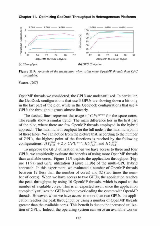
Chapter 11. Optimizing GeoDock Throughput in Heterogeneous Platforms
5
6
7
8
9
12 16 20 24 28 32Thro
ug
hp
ut
[Lig
and
s/se
c]
#OpenMP Threads in Hybrid
2 GPU 3 GPU 4 GPU
(a) Throughput
70
75
80
85
90
95
100
12 16 20 24 28 32
Uti
lizati
on (
%)
#OpenMP Threads in Hybrid
2 GPU 3 GPU 4 GPU
(b) GPU Utilization
Figure 11.9: Analysis of the application when using more OpenMP threads than CPUavailables.
Source: [207]
OpenMP threads we considered, the GPUs are under-utilized. In particular,the GeoDock configurations that use 3 GPUs are slowing down a bit onlyin the last part of the plot, while in the GeoDock configurations that use 4GPUs the throughput grows almost linearly.
The dashed lines represent the usage of CPUproc for the spare cores.The results show a similar trend. The main difference lies in the first partof the plot, where there are few OpenMP threads employed in the hybridapproach. The maximum throughput for the full node is the maximum pointof these lines. We can notice from the picture that, according to the numberof GPUs, the highest point of the functions is reached by the followingconfigurations: HY proc
14,2 + 2× CPUproc, HY proc16,3 , and HY proc
16,4 .To improve the GPU utilization when we have access to three and four
GPUs, we empirically evaluate the benefits of using more OpenMP threadsthan available cores. Figure 11.9 depicts the application throughput (Fig-ure 11.9a) and GPU utilization (Figure 11.9b) of the multi-GPU hybridapproach. In this experiment, we evaluated a number of OpenMP threadsbetween 12 (less than the number of cores) and 32 (two times the num-ber of cores). When we have access to two GPUs, the application reachesthe peak throughput by using 16 OpenMP threads, which is equal to thenumber of available cores. This is an expected result since the applicationcompletely utilizes the GPUs without overloading the system with OpenMPthreads. However, when we have access to more than two GPUs, the appli-cation reaches the peak throughput by using a number of OpenMP threadsgreater than the available cores. This benefit is due to the increased utiliza-tion of GPUs. Indeed, the operating system can serve an available worker
172
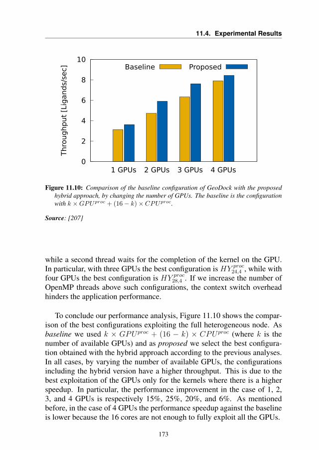
11.4. Experimental Results
0
2
4
6
8
10
1 GPUs 2 GPUs 3 GPUs 4 GPUs
Thro
ug
hp
ut
[Lig
and
s/se
c] Baseline Proposed
Figure 11.10: Comparison of the baseline configuration of GeoDock with the proposedhybrid approach, by changing the number of GPUs. The baseline is the configurationwith k ×GPUproc + (16− k)× CPUproc.
Source: [207]
while a second thread waits for the completion of the kernel on the GPU.In particular, with three GPUs the best configuration is HY proc
24,4 , while withfour GPUs the best configuration is HY proc
28,4 . If we increase the number ofOpenMP threads above such configurations, the context switch overheadhinders the application performance.
To conclude our performance analysis, Figure 11.10 shows the compar-ison of the best configurations exploiting the full heterogeneous node. Asbaseline we used k × GPUproc + (16 − k) × CPUproc (where k is thenumber of available GPUs) and as proposed we select the best configura-tion obtained with the hybrid approach according to the previous analyses.In all cases, by varying the number of available GPUs, the configurationsincluding the hybrid version have a higher throughput. This is due to thebest exploitation of the GPUs only for the kernels where there is a higherspeedup. In particular, the performance improvement in the case of 1, 2,3, and 4 GPUs is respectively 15%, 25%, 20%, and 6%. As mentionedbefore, in the case of 4 GPUs the performance speedup against the baselineis lower because the 16 cores are not enough to fully exploit all the GPUs.
173
Chapter 11. Optimizing GeoDock Throughput in Heterogeneous Platforms
11.5 Summary
Working with heterogeneous platforms introduces more complexity whenwriting applications since the programmer needs to consider the creationof kernels for the accelerators and how to distribute the computations thathave to be performed across the different hardware. This is even morecomplex since the different hardware have different characteristics, and thedeveloper needs to consider those characteristics when designing the appli-cations and selecting which kernel will run where.
In this chapter, we have seen how it is possible to further optimize theGeoDock application that we have seen in the previous chapter. In partic-ular, we have seen how, thanks to an improved organization of the compu-tation and on the selection of the more suitable platform for the differentkernel, we were able to improve the throughput of GeoDock (up to 25%)without changing the underlying architecture.
The outcome of this work has been published in the Journal of Super-computing [207].
174
CHAPTER12Improving GeoDock GPU efficiency with
Cuda and Dynamic Kernel Tuning
With the rise of the COVID19 pandemic, the GeoDock application (de-scribed in Section 8) needed to be further optimized to be usable in thesearch for a drug to find a therapeutic cure against the virus. In this chap-ter we will show a porting of GeoDock to a newer supercomputer, with amore powerful GPU component, and we will optimize the application withCUDA in order to obtain the most from the powerful V100 GPGPU. Thislead to a drastic improvement in the performances (more than 3x). More-over we introduce some data-driven autotuning in the application that allowus to avoid some not needed computation, further improving the speedupunder certain circumstances.
The work described in this chapter has been carried out as part of theExscalate4COVID European project, and since GeoDock is a key compo-nent in the EXSCALATE pipeline for drug discovery, it was fundamentalfor the largest virtual screening ever performed (November 2020) [208].
175
Chapter 12. Improving GeoDock GPU efficiency with Cuda and DynamicKernel Tuning
12.1 Introduction
The SARS-COV2 pandemic has created new challenges for the whole world,which had to put a lot of effort into researching a way to contrast the spreadof the epidemy. In this context, we insert our effort spent in improving theperformance of GeoDock. The application is needed to perform a large vir-tual screening campaign to find potential candidate drugs that can contrastthe virus. However, to manage such a large number of candidates (in theorder of billions) in a reasonable time we need to improve the capabilitiesof the application itself. Moreover, knowing beforehand the target plat-form capabilities (Marconi100 supercomputer from CINECA and HPC5from ENI) allows us to make some decisions in the porting of the applica-tion, that has been tailored for those machine architectures. In particular,since both of them are heterogeneous machines, with the same GPU accel-erator (the NVIDIA V100 GPGPU cards), we decided to rewrite the mostcompute-intensive kernels from OpenACC to CUDA, to harness the fullpower of the GPU.
From the autotuning point of view, we inserted in the main algorithmsome knowledge that makes it able to select at runtime the number of itera-tion (and thus, the dimension of the CUDA grids). This mechanism exploitssome features of the data (and of the docking algorithm) to optimize, with-out loss of precision, the execution time. For this reason, we classify it asproactive autotuning.
Thus the contributions of this chapter are:
• An in-depth analysis of the porting from OpenACC to CUDA of theimportant kernels of GeoDock.
• The introduction of the proactive autotuning in the application.
In the context of the global framework, this chapter provides a workingexample of a heterogenous autotuning module.
The components of the framework that are involved in this chapter canbe seen in Figure 12.1. We can notice the GPU kernel presence since thekey point of this work is the automatic tunability of those kernels. We usethe data feature to select the kernel grid parameters, thus creating a realdynamic application that will change its configuration according to its datainput.
176
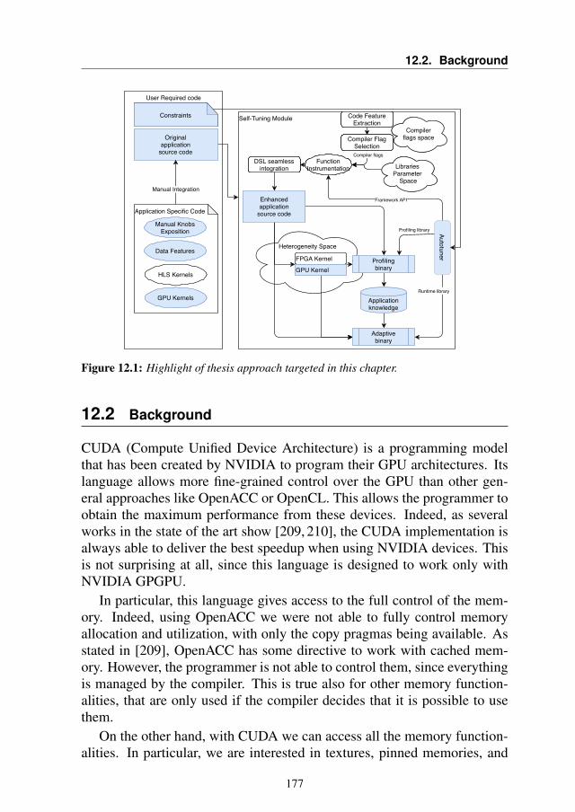
12.2. Background
User Required code
Self-Tuning Module
Heterogeneity Space
Originalapplication
source code
Code FeatureExtraction
Compilerflags space
Compiler flags
Compiler FlagSelection
Libraries Parameter
Space
DSL seamlessintegration
Enhancedapplication
source code
Profilingbinary
Applicationknowledge
Adaptivebinary
Runtime library
Framework API
Autotuner
Profiling library
Manual Integration
Application Specific Code
Data Features
HLS Kernels
GPU Kernels
FPGA Kernel
GPU Kernel
Constraints
Manual KnobsExposition
FunctionInstrumentation
Constraints Code FeatureExtraction
Compiler FlagSelection
FunctionInstrumentation Libraries
Parameter Space
Compilerflags space
DSL seamlessintegration
Autotuner
Figure 12.1: Highlight of thesis approach targeted in this chapter.
12.2 Background
CUDA (Compute Unified Device Architecture) is a programming modelthat has been created by NVIDIA to program their GPU architectures. Itslanguage allows more fine-grained control over the GPU than other gen-eral approaches like OpenACC or OpenCL. This allows the programmer toobtain the maximum performance from these devices. Indeed, as severalworks in the state of the art show [209, 210], the CUDA implementation isalways able to deliver the best speedup when using NVIDIA devices. Thisis not surprising at all, since this language is designed to work only withNVIDIA GPGPU.
In particular, this language gives access to the full control of the mem-ory. Indeed, using OpenACC we were not able to fully control memoryallocation and utilization, with only the copy pragmas being available. Asstated in [209], OpenACC has some directive to work with cached mem-ory. However, the programmer is not able to control them, since everythingis managed by the compiler. This is true also for other memory function-alities, that are only used if the compiler decides that it is possible to usethem.
On the other hand, with CUDA we can access all the memory function-alities. In particular, we are interested in textures, pinned memories, and
177
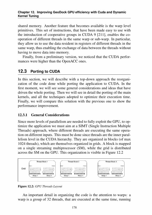
Chapter 12. Improving GeoDock GPU efficiency with Cuda and DynamicKernel Tuning
shared memory. Another feature that becomes available is the warp levelprimitives. This set of instructions, that have been made easy to use withthe introduction of cooperative groups in CUDA 9 [211], enables the co-operation of different threads in the same warp or sub-warp. In particular,they allow us to use the data resident in registers of different threads in thesame warp, thus enabling the exchange of data between the threads withouthaving to move data into memory.
Finally, from a preliminary version, we noticed that the CUDA perfor-mances were higher than the OpenACC ones.
12.3 Porting to CUDA
In this section, we will describe with a top-down approach the reorgani-zation of the code done while porting the application to CUDA. In thefirst moment, we will see some general considerations and ideas that havedriven the whole porting. Then we will see in detail the porting of the mainkernels, and all the techniques adopted to optimize their execution time.Finally, we will compare this solution with the previous one to show theperformance improvement.
12.3.1 General Considerations
Since more levels of parallelism are needed to fully exploit the GPU, to op-timize the application we must aim at a SIMT (Single Instruction MultipleThreads) approach, where different threads are executing the same opera-tion on different inputs. This must be done since threads are the inner paral-lelism level in the CUDA hierarchy. They are organized in blocks (of max1024 threads), which are themselves organized in grids. A block is mappedon a single streaming multiprocessor (SM), while the grid is distributedacross the SM on the GPU. This organization is visible in Figure 12.2
Figure 12.2: GPU Threads Layout
An important detail in organizing the code is the attention to warps: awarp is a group of 32 threads, that are executed at the same time, running
178
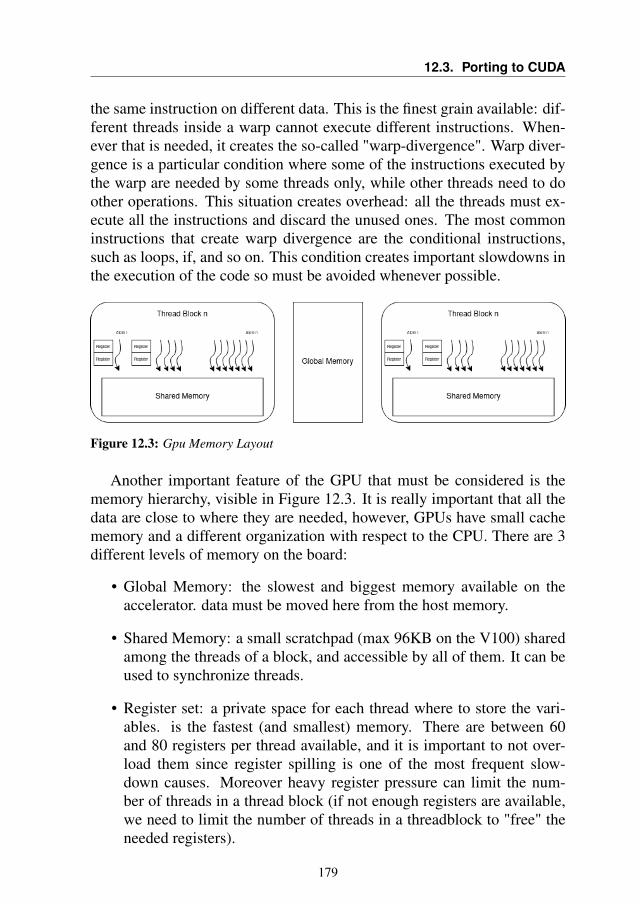
12.3. Porting to CUDA
the same instruction on different data. This is the finest grain available: dif-ferent threads inside a warp cannot execute different instructions. When-ever that is needed, it creates the so-called "warp-divergence". Warp diver-gence is a particular condition where some of the instructions executed bythe warp are needed by some threads only, while other threads need to doother operations. This situation creates overhead: all the threads must ex-ecute all the instructions and discard the unused ones. The most commoninstructions that create warp divergence are the conditional instructions,such as loops, if, and so on. This condition creates important slowdowns inthe execution of the code so must be avoided whenever possible.
Figure 12.3: Gpu Memory Layout
Another important feature of the GPU that must be considered is thememory hierarchy, visible in Figure 12.3. It is really important that all thedata are close to where they are needed, however, GPUs have small cachememory and a different organization with respect to the CPU. There are 3different levels of memory on the board:
• Global Memory: the slowest and biggest memory available on theaccelerator. data must be moved here from the host memory.
• Shared Memory: a small scratchpad (max 96KB on the V100) sharedamong the threads of a block, and accessible by all of them. It can beused to synchronize threads.
• Register set: a private space for each thread where to store the vari-ables. is the fastest (and smallest) memory. There are between 60and 80 registers per thread available, and it is important to not over-load them since register spilling is one of the most frequent slow-down causes. Moreover heavy register pressure can limit the num-ber of threads in a thread block (if not enough registers are available,we need to limit the number of threads in a threadblock to "free" theneeded registers).
179
Chapter 12. Improving GeoDock GPU efficiency with Cuda and DynamicKernel Tuning
On the application side, the main challenge is the reorganization of thecomputation, to maximize the parallelism, while keeping the computationbalanced. We have already found three different levels of parallelism inthe application, as can be seen in Chapter 10 and Chapter 11. These par-allelism levels allow us to target the multinode machine, and to distributethe computation across different nodes with limited impact of communi-cation on the performances. The outer level is the number of candidateligands to evaluate: since this number is in the order of billions, we canconsider this problem embarrassingly parallel. This allows us to distributethe ligands across the different nodes and cores of the supercomputer, witha very small communication overhead (we do not need to synchronize thenodes during the runtime, but only at the beginning and at the end of thecomputation). The intermediate level is due to the adopted docking algo-rithm: multiple restarts where every restart has a different starting pose.For this reason, all the poses are independent and can be evaluated in par-allel. Indeed, besides the initial situation, even at this level all the data canbe considered independent and don’t need synchronization before the finalscore evaluation phase, where the best-scored pose is selected. The innerlevel of parallelism is given by the atoms: every ligand is composed of sev-eral atoms that are moved according to some rotations and translation. Thisis the SIMT approach that we are searching for since the same instruction(rotate or translate) is applied to different data (the atoms). Moreover, weneed to give strong attention to memory organization. We aim at reducingto the minimum the number of expensive operations (such as data trans-fer, memory allocation, and deallocation). Meanwhile, we need to keep thedata as close as possible to the compute units.
To optimize the utilization of the GPU accelerators, they are sharedamong different threads, asynchronously. Every ligand will be tied to athread, that is tied to an asynchronous queue and a reserved space in theGPU memory. The reservation of the space at thread level instead of atligand level allows us to allocate and deallocate that memory only once inthe lifetime of the thread. This is a first optimization that allows savinga lot of memory operations, since this memory space is not linked to thedocking of a single ligand, but is linked to the lifetime of the application.The drawback of this approach is that we need to allocate the worst casespace, and this must be known at compile-time. This introduces a limitationon the maximum size of the processed ligands. However, this is not a realissue in the application since it can be changed at compile time. Moreover,some data structures (such as the pocket space) can be shared among all thethreads that are using the same GPU: this can be done since they are read-
180
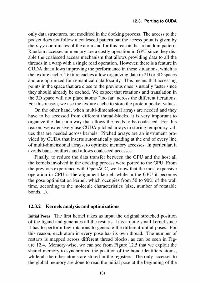
12.3. Porting to CUDA
only data structures, not modified in the docking process. The access to thepocket does not follow a coalesced pattern but the access point is given bythe x,y,z coordinates of the atom and for this reason, has a random pattern.Random accesses in memory are a costly operation in GPU since they dis-able the coalesced access mechanism that allows providing data to all thethreads in a warp with a single read operation. However, there is a feature inCUDA that allows improving the performance in these situations, which isthe texture cache. Texture caches allow organizing data in 2D or 3D spacesand are optimized for semantical data locality. This means that accessingpoints in the space that are close to the previous ones is usually faster sincethey should already be cached. We expect that rotations and translation inthe 3D space will not place atoms "too far" across the different iterations.For this reason, we use the texture cache to store the protein pocket values.
On the other hand, when multi-dimensional arrays are needed and theyhave to be accessed from different thread-blocks, it is very important toorganize the data in a way that allows the reads to be coalesced. For thisreason, we extensively use CUDA pitched arrays in storing temporary val-ues that are needed across kernels. Pitched arrays are an instrument pro-vided by CUDA that inserts automatically padding at the end of every lineof multi-dimensional arrays, to optimize memory accesses. In particular, itavoids bank-conflicts and allows coalesced accesses.
Finally, to reduce the data transfer between the GPU and the host allthe kernels involved in the docking process were ported to the GPU. Fromthe previous experience with OpenACC, we know that the most expensiveoperation in CPU is the alignment kernel, while in the GPU it becomesthe pose optimization kernel, which occupies from 50 to 90% of the walltime, according to the molecule characteristics (size, number of rotatablebonds,...).
12.3.2 Kernels analysis and optimizations
Initial Poses The first kernel takes as input the original stretched positionof the ligand and generates all the restarts. It is a quite small kernel sinceit has to perform few rotations to generate the different initial poses. Forthis reason, each atom in every pose has its own thread. The number ofrestarts is mapped across different thread blocks, as can be seen in Fig-ure 12.4. Memory-wise, we can see from Figure 12.5 that we exploit theshared memory to synchronize the position of the bond identifiers atoms,while all the other atoms are stored in the registers. The only accesses tothe global memory are done to read the initial pose at the beginning of the
181
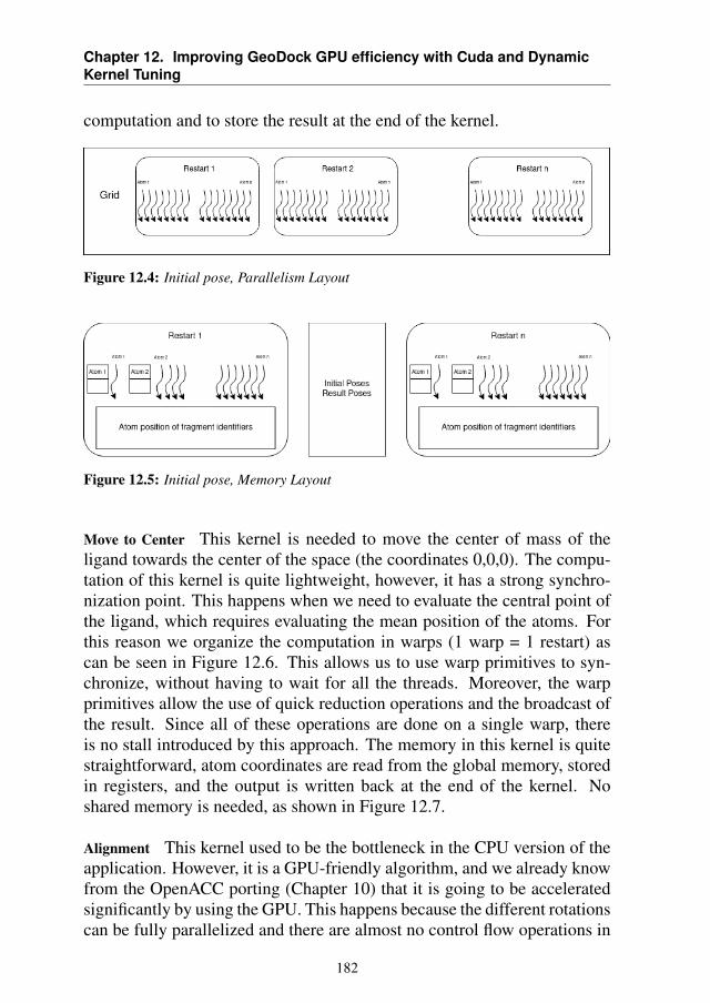
Chapter 12. Improving GeoDock GPU efficiency with Cuda and DynamicKernel Tuning
computation and to store the result at the end of the kernel.
Figure 12.4: Initial pose, Parallelism Layout
Figure 12.5: Initial pose, Memory Layout
Move to Center This kernel is needed to move the center of mass of theligand towards the center of the space (the coordinates 0,0,0). The compu-tation of this kernel is quite lightweight, however, it has a strong synchro-nization point. This happens when we need to evaluate the central point ofthe ligand, which requires evaluating the mean position of the atoms. Forthis reason we organize the computation in warps (1 warp = 1 restart) ascan be seen in Figure 12.6. This allows us to use warp primitives to syn-chronize, without having to wait for all the threads. Moreover, the warpprimitives allow the use of quick reduction operations and the broadcast ofthe result. Since all of these operations are done on a single warp, thereis no stall introduced by this approach. The memory in this kernel is quitestraightforward, atom coordinates are read from the global memory, storedin registers, and the output is written back at the end of the kernel. Noshared memory is needed, as shown in Figure 12.7.
Alignment This kernel used to be the bottleneck in the CPU version of theapplication. However, it is a GPU-friendly algorithm, and we already knowfrom the OpenACC porting (Chapter 10) that it is going to be acceleratedsignificantly by using the GPU. This happens because the different rotationscan be fully parallelized and there are almost no control flow operations in
182

12.3. Porting to CUDA
Figure 12.6: Move to center, Parallelism Layout
Figure 12.7: Move to center, Memory Layout
the algorithm. Moreover, to maximize the distribution of the computations,we divided the alignment phase into 3 different kernels:
1. Score evaluation and reduction to obtain the maximum score. Thereduction can manage a maximum of 1024 angles. The limit to thenumber of angles is due to the fact that every thread evaluates an angle,and the max number of threads per block is 1024.
2. If more than 1024 angles are being tested in a single pose, a reductionkernel is in charge of selecting the best angle.
3. The final kernel is in charge of placing the molecule with the anglethat was showing the best score.
Using this organization, we can have different parallelism and a better bal-ancing among the threads.
Evaluate Score This is the main kernel of the alignment phase, wheremost of the computations are done. Since there are quite a lot of evaluationsto be performed, we map a full rotation on a single thread, that evaluatesthe rotation matrix and applies it to all the atoms of the ligand. With thisorganization up to 1024 angles can be evaluated in a thread block, as canbe seen in Figure 12.8. For this reason, it is possible that more than 1thread block handles a restart. If this happens, we need kernel number 2(the reduction kernel), otherwise, that kernel can be skipped.
183
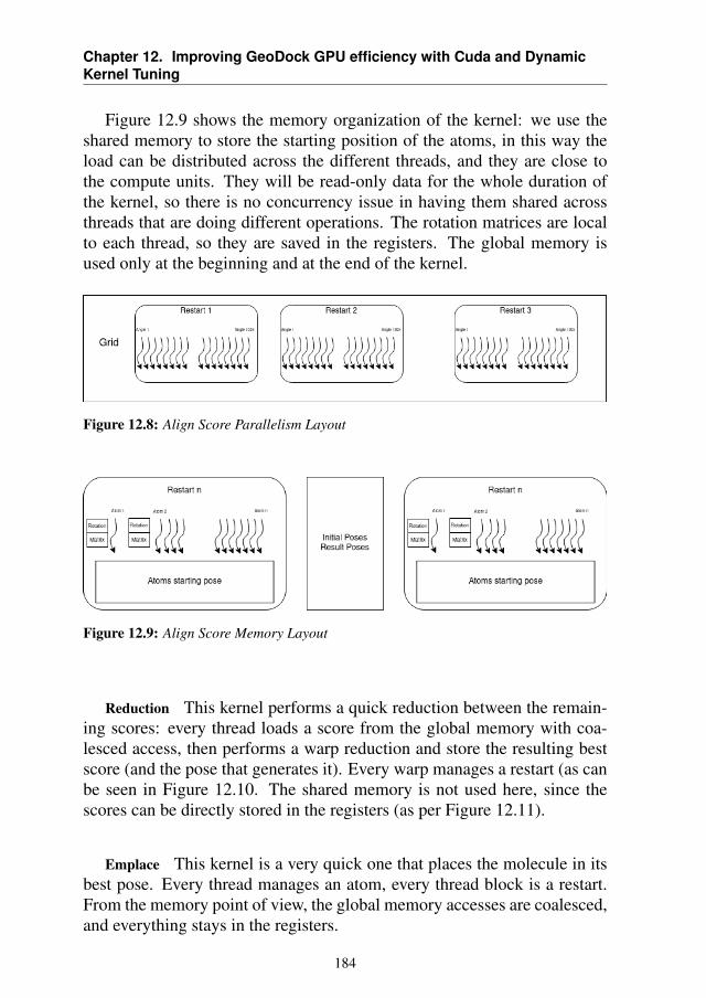
Chapter 12. Improving GeoDock GPU efficiency with Cuda and DynamicKernel Tuning
Figure 12.9 shows the memory organization of the kernel: we use theshared memory to store the starting position of the atoms, in this way theload can be distributed across the different threads, and they are close tothe compute units. They will be read-only data for the whole duration ofthe kernel, so there is no concurrency issue in having them shared acrossthreads that are doing different operations. The rotation matrices are localto each thread, so they are saved in the registers. The global memory isused only at the beginning and at the end of the kernel.
Figure 12.8: Align Score Parallelism Layout
Figure 12.9: Align Score Memory Layout
Reduction This kernel performs a quick reduction between the remain-ing scores: every thread loads a score from the global memory with coa-lesced access, then performs a warp reduction and store the resulting bestscore (and the pose that generates it). Every warp manages a restart (as canbe seen in Figure 12.10. The shared memory is not used here, since thescores can be directly stored in the registers (as per Figure 12.11).
Emplace This kernel is a very quick one that places the molecule in itsbest pose. Every thread manages an atom, every thread block is a restart.From the memory point of view, the global memory accesses are coalesced,and everything stays in the registers.
184
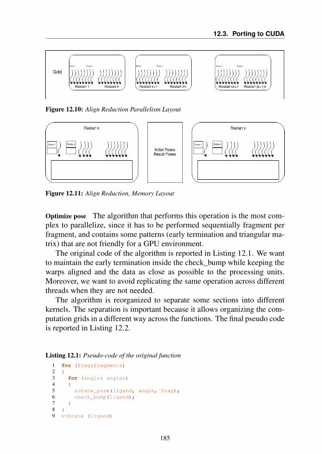
12.3. Porting to CUDA
Figure 12.10: Align Reduction Parallelism Layout
Figure 12.11: Align Reduction, Memory Layout
Optimize pose The algorithm that performs this operation is the most com-plex to parallelize, since it has to be performed sequentially fragment perfragment, and contains some patterns (early termination and triangular ma-trix) that are not friendly for a GPU environment.
The original code of the algorithm is reported in Listing 12.1. We wantto maintain the early termination inside the check_bump while keeping thewarps aligned and the data as close as possible to the processing units.Moreover, we want to avoid replicating the same operation across differentthreads when they are not needed.
The algorithm is reorganized to separate some sections into differentkernels. The separation is important because it allows organizing the com-putation grids in a different way across the functions. The final pseudo codeis reported in Listing 12.2.
Listing 12.1: Pseudo-code of the original function1 for (frag:fragments)2 {3 for (angle: angles)4 {5 rotate_pose(ligand, angle, frag);6 check_bump(ligand);7 }8 }9 vibrate (ligand)
185
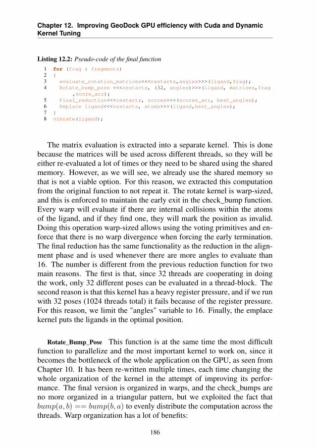
Chapter 12. Improving GeoDock GPU efficiency with Cuda and DynamicKernel Tuning
Listing 12.2: Pseudo-code of the final function1 for (frag : fragments)2 {3 evaluate_rotation_matrices<<<restarts,angles>>>(ligand,frag);4 Rotate_bump_pose <<<restarts, (32, angles)>>>(ligand, matrices,frag
,score_arr);5 Final_reduction<<<restarts, scores>>>(scores_arr, best_angles);6 Emplace ligand<<<restarts, atoms>>>(ligand,best_angles);7 }8 vibrate(ligand);
The matrix evaluation is extracted into a separate kernel. This is donebecause the matrices will be used across different threads, so they will beeither re-evaluated a lot of times or they need to be shared using the sharedmemory. However, as we will see, we already use the shared memory sothat is not a viable option. For this reason, we extracted this computationfrom the original function to not repeat it. The rotate kernel is warp-sized,and this is enforced to maintain the early exit in the check_bump function.Every warp will evaluate if there are internal collisions within the atomsof the ligand, and if they find one, they will mark the position as invalid.Doing this operation warp-sized allows using the voting primitives and en-force that there is no warp divergence when forcing the early termination.The final reduction has the same functionality as the reduction in the align-ment phase and is used whenever there are more angles to evaluate than16. The number is different from the previous reduction function for twomain reasons. The first is that, since 32 threads are cooperating in doingthe work, only 32 different poses can be evaluated in a thread-block. Thesecond reason is that this kernel has a heavy register pressure, and if we runwith 32 poses (1024 threads total) it fails because of the register pressure.For this reason, we limit the "angles" variable to 16. Finally, the emplacekernel puts the ligands in the optimal position.
Rotate_Bump_Pose This function is at the same time the most difficultfunction to parallelize and the most important kernel to work on, since itbecomes the bottleneck of the whole application on the GPU, as seen fromChapter 10. It has been re-written multiple times, each time changing thewhole organization of the kernel in the attempt of improving its perfor-mance. The final version is organized in warps, and the check_bumps areno more organized in a triangular pattern, but we exploited the fact thatbump(a, b) == bump(b, a) to evenly distribute the computation across thethreads. Warp organization has a lot of benefits:
186
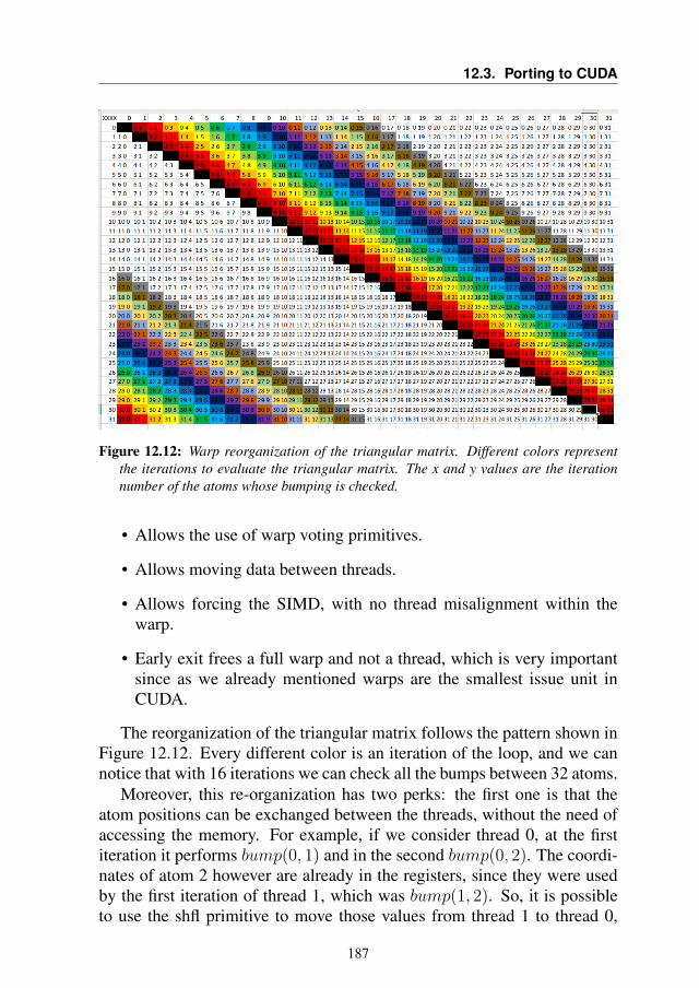
12.3. Porting to CUDA
Figure 12.12: Warp reorganization of the triangular matrix. Different colors representthe iterations to evaluate the triangular matrix. The x and y values are the iterationnumber of the atoms whose bumping is checked.
• Allows the use of warp voting primitives.
• Allows moving data between threads.
• Allows forcing the SIMD, with no thread misalignment within thewarp.
• Early exit frees a full warp and not a thread, which is very importantsince as we already mentioned warps are the smallest issue unit inCUDA.
The reorganization of the triangular matrix follows the pattern shown inFigure 12.12. Every different color is an iteration of the loop, and we cannotice that with 16 iterations we can check all the bumps between 32 atoms.
Moreover, this re-organization has two perks: the first one is that theatom positions can be exchanged between the threads, without the need ofaccessing the memory. For example, if we consider thread 0, at the firstiteration it performs bump(0, 1) and in the second bump(0, 2). The coordi-nates of atom 2 however are already in the registers, since they were usedby the first iteration of thread 1, which was bump(1, 2). So, it is possibleto use the shfl primitive to move those values from thread 1 to thread 0,
187
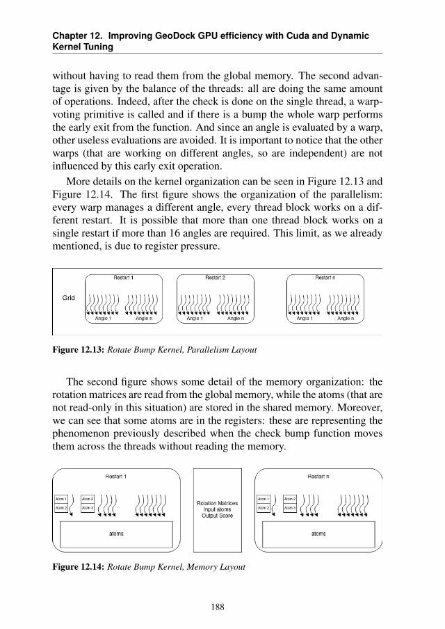
Chapter 12. Improving GeoDock GPU efficiency with Cuda and DynamicKernel Tuning
without having to read them from the global memory. The second advan-tage is given by the balance of the threads: all are doing the same amountof operations. Indeed, after the check is done on the single thread, a warp-voting primitive is called and if there is a bump the whole warp performsthe early exit from the function. And since an angle is evaluated by a warp,other useless evaluations are avoided. It is important to notice that the otherwarps (that are working on different angles, so are independent) are notinfluenced by this early exit operation.
More details on the kernel organization can be seen in Figure 12.13 andFigure 12.14. The first figure shows the organization of the parallelism:every warp manages a different angle, every thread block works on a dif-ferent restart. It is possible that more than one thread block works on asingle restart if more than 16 angles are required. This limit, as we alreadymentioned, is due to register pressure.
Figure 12.13: Rotate Bump Kernel, Parallelism Layout
The second figure shows some detail of the memory organization: therotation matrices are read from the global memory, while the atoms (that arenot read-only in this situation) are stored in the shared memory. Moreover,we can see that some atoms are in the registers: these are representing thephenomenon previously described when the check bump function movesthem across the threads without reading the memory.
Figure 12.14: Rotate Bump Kernel, Memory Layout
188
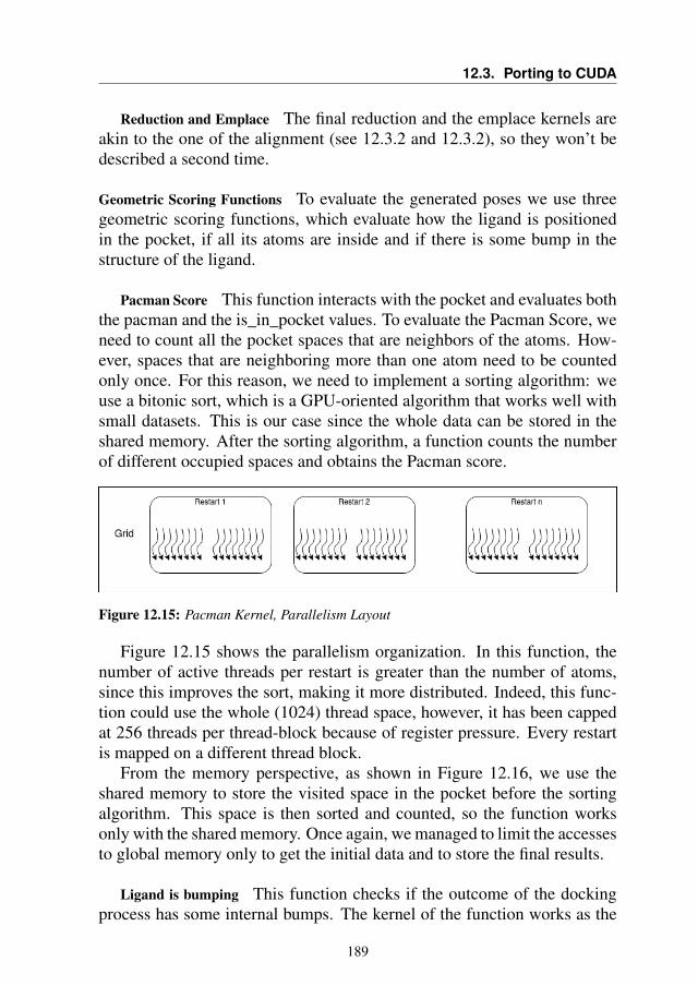
12.3. Porting to CUDA
Reduction and Emplace The final reduction and the emplace kernels areakin to the one of the alignment (see 12.3.2 and 12.3.2), so they won’t bedescribed a second time.
Geometric Scoring Functions To evaluate the generated poses we use threegeometric scoring functions, which evaluate how the ligand is positionedin the pocket, if all its atoms are inside and if there is some bump in thestructure of the ligand.
Pacman Score This function interacts with the pocket and evaluates boththe pacman and the is_in_pocket values. To evaluate the Pacman Score, weneed to count all the pocket spaces that are neighbors of the atoms. How-ever, spaces that are neighboring more than one atom need to be countedonly once. For this reason, we need to implement a sorting algorithm: weuse a bitonic sort, which is a GPU-oriented algorithm that works well withsmall datasets. This is our case since the whole data can be stored in theshared memory. After the sorting algorithm, a function counts the numberof different occupied spaces and obtains the Pacman score.
Figure 12.15: Pacman Kernel, Parallelism Layout
Figure 12.15 shows the parallelism organization. In this function, thenumber of active threads per restart is greater than the number of atoms,since this improves the sort, making it more distributed. Indeed, this func-tion could use the whole (1024) thread space, however, it has been cappedat 256 threads per thread-block because of register pressure. Every restartis mapped on a different thread block.
From the memory perspective, as shown in Figure 12.16, we use theshared memory to store the visited space in the pocket before the sortingalgorithm. This space is then sorted and counted, so the function worksonly with the shared memory. Once again, we managed to limit the accessesto global memory only to get the initial data and to store the final results.
Ligand is bumping This function checks if the outcome of the dockingprocess has some internal bumps. The kernel of the function works as the
189
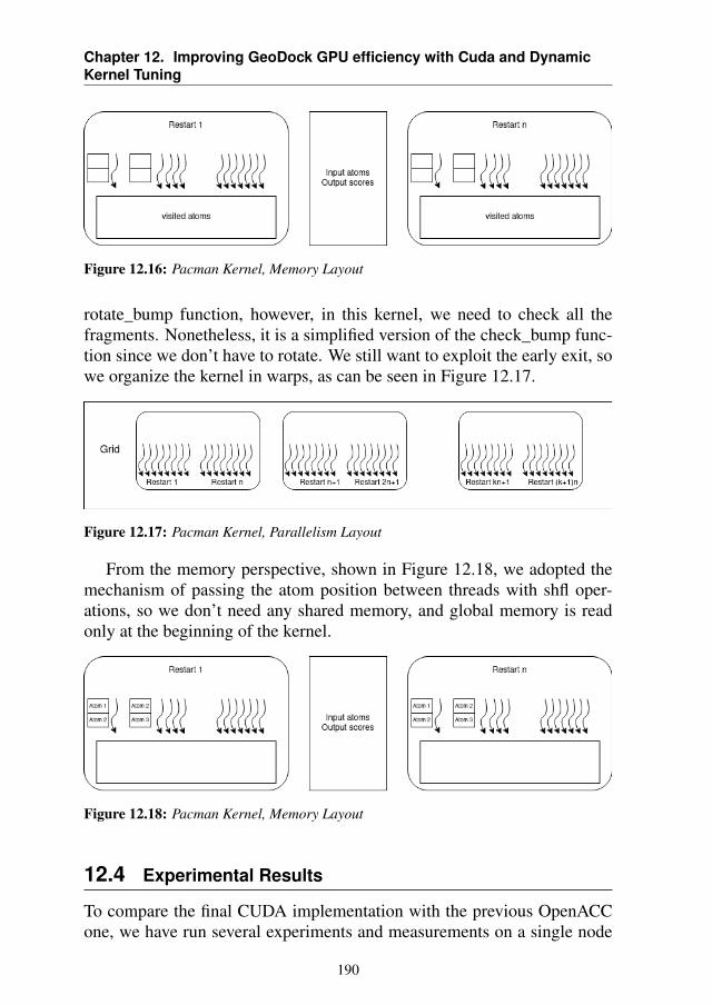
Chapter 12. Improving GeoDock GPU efficiency with Cuda and DynamicKernel Tuning
Figure 12.16: Pacman Kernel, Memory Layout
rotate_bump function, however, in this kernel, we need to check all thefragments. Nonetheless, it is a simplified version of the check_bump func-tion since we don’t have to rotate. We still want to exploit the early exit, sowe organize the kernel in warps, as can be seen in Figure 12.17.
Figure 12.17: Pacman Kernel, Parallelism Layout
From the memory perspective, shown in Figure 12.18, we adopted themechanism of passing the atom position between threads with shfl oper-ations, so we don’t need any shared memory, and global memory is readonly at the beginning of the kernel.
Figure 12.18: Pacman Kernel, Memory Layout
12.4 Experimental Results
To compare the final CUDA implementation with the previous OpenACCone, we have run several experiments and measurements on a single node
190
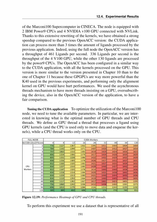
12.4. Experimental Results
of the Marconi100 Supercomputer in CINECA. The node is equipped with2 IBM Power9 CPUs and 4 NVIDIA v100 GPU connected with NVLink.Thanks to this extensive rewriting of the kernels, we have obtained a strongspeedup compared to the previous OpenACC version: the CUDA applica-tion can process more than 3 times the amount of ligands processed by theprevious application. Indeed, using the full node the OpenACC version hasa throughput of 461 Ligands per second. 336 Ligands per second is thethroughput of the 4 V100 GPU, while the other 130 ligands are processedby the power9 CPUs. The OpenACC has been configured in a similar wayto the CUDA application, with all the kernels processed on the GPU. Thisversion is more similar to the version presented in Chapter 10 than to theone of Chapter 11 because these GPGPUs are way more powerful than theK40 used in the previous experiments, and performing only the alignmentkernel on GPU would have hurt performances. We used the asynchronousthreads mechanism to have more threads insisting on a GPU, oversubscrib-ing the device, also in the OpenACC version of the application, to have afair comparison.
Tuning the CUDA application To optimize the utilization of the Marconi100node, we need to tune the available parameters. In particular, we are inter-ested in knowing what is the optimal number of GPU threads and CPUthreads. We define as GPU thread a thread that processes a ligand usingGPU kernels (and the CPU is used only to move data and enqueue the ker-nels), while a CPU thread works only on the CPU.
Figure 12.19: Performance Heatmap of GPU and CPU threads.
To perform this experiment we use a dataset that is representative of all
191
Chapter 12. Improving GeoDock GPU efficiency with Cuda and DynamicKernel Tuning
the possible ligands’ size and fragment numbers, since we need to staticallysetup the amount of workers before running the experiments. In this way,we can avoid to repeat this effort when we change the dataset. We will seein the following section an orthogonal technique to optimize the applicationconsidering input characteristics. Figure 12.19 shows the outcome of thedesign space exploration done. On the columns, we report the number ofGPU threads allocated for the job, while the rows have the CPU threads. Wecan notice that the total amount of threads can be more than the availablethreads on the Power9 processors since we are open to the possibility thatoversubscription and hyperthreading could bring some benefit. However,from the results of the experiment, we can notice that this hypothesis isnot true, since the optimal points on the heatmap are around 64GPU and20CPU threads, which are less than the number of logical cores availableon the node. Nonetheless, the hyperthreading approach is correct, sincethe optimal point has more thread than the number of physical cores of thenode.
Finally, thanks to this CUDA porting, we were able to increase thethroughput by 1000 ligands per second, on the same dataset. Indeed, thetotal throughput of the node was 1445 ligands per second: the porting pro-vided a speedup of more than 3x compared to the OpenACC version ofChapter 10.
12.5 Autotuning
Even if autotuning is not the focal point of this chapter, we believe that ispossible to further speed up the application by applying the techniques de-veloped in the previous chapters. In particular, we analyzed the applicationand noticed that there is an important data dependency that, if addressedcorrectly, can allow the application to save some operations. In particular,it is a repetition of the evaluation of some poses that happens wheneverthere are not enough fragments in the ligand to generate the initial poses.These repetitions are not improving the accuracy of the result but they areonly performing the same pose evaluation more times, so it is desirable toavoid them. We applied the technique developed in Chapter 6, to proac-tively select the number of poses to test. In particular, we used the numberof fragments as data-feature and the number of poses as software knob. Itis important to notice that this software knob strongly influences the ap-plication since for several kernels it is involved in the grid organization.Indeed, by changing this parameter the dimension of the CUDA grids areeffectively modified, and the amount of calculation required to obtain the
192
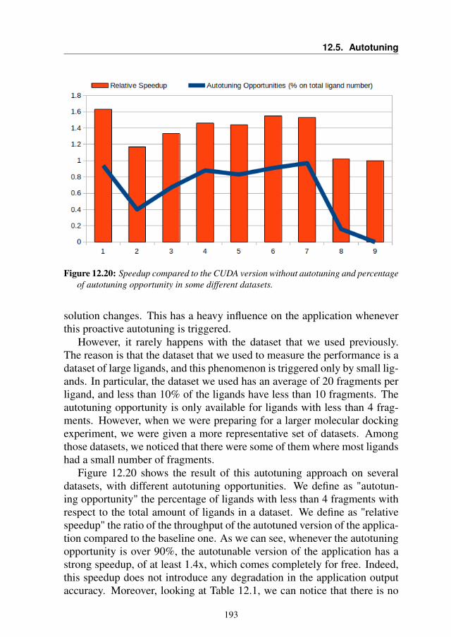
12.5. Autotuning
Figure 12.20: Speedup compared to the CUDA version without autotuning and percentageof autotuning opportunity in some different datasets.
solution changes. This has a heavy influence on the application wheneverthis proactive autotuning is triggered.
However, it rarely happens with the dataset that we used previously.The reason is that the dataset that we used to measure the performance is adataset of large ligands, and this phenomenon is triggered only by small lig-ands. In particular, the dataset we used has an average of 20 fragments perligand, and less than 10% of the ligands have less than 10 fragments. Theautotuning opportunity is only available for ligands with less than 4 frag-ments. However, when we were preparing for a larger molecular dockingexperiment, we were given a more representative set of datasets. Amongthose datasets, we noticed that there were some of them where most ligandshad a small number of fragments.
Figure 12.20 shows the result of this autotuning approach on severaldatasets, with different autotuning opportunities. We define as "autotun-ing opportunity" the percentage of ligands with less than 4 fragments withrespect to the total amount of ligands in a dataset. We define as "relativespeedup" the ratio of the throughput of the autotuned version of the applica-tion compared to the baseline one. As we can see, whenever the autotuningopportunity is over 90%, the autotunable version of the application has astrong speedup, of at least 1.4x, which comes completely for free. Indeed,this speedup does not introduce any degradation in the application outputaccuracy. Moreover, looking at Table 12.1, we can notice that there is no
193
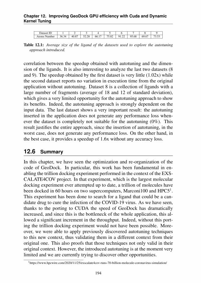
Chapter 12. Improving GeoDock GPU efficiency with Cuda and DynamicKernel Tuning
Dataset ID 1 2 3 4 5 6 7 8 9Atoms Number 36.34 40.87 52.28 66.17 75.82 91.22 95.68 69.67 73.53
Table 12.1: Average size of the ligand of the datasets used to explore the autotuningapproach introduced.
correlation between the speedup obtained with autotuning and the dimen-sion of the ligands. It is also interesting to analyze the last two datasets (8and 9). The speedup obtained by the first dataset is very little (1.02x) whilethe second dataset reports no variation in execution time from the originalapplication without autotuning. Dataset 8 is a collection of ligands with alarge number of fragments (average of 18 and 12 of standard deviation),which gives a very limited opportunity for the autotuning approach to showits benefits. Indeed, the autotuning approach is strongly dependent on theinput data. The last dataset shows a very important result: the autotuninginserted in the application does not generate any performance loss when-ever the dataset is completely not suitable for the autotuning (0%). Thisresult justifies the entire approach, since the insertion of autotuning, in theworst case, does not generate any performance loss. On the other hand, inthe best case, it provides a speedup of 1.6x without any accuracy loss.
12.6 Summary
In this chapter, we have seen the optimization and re-organization of thecode of GeoDock. In particular, this work has been fundamental in en-abling the trillion docking experiment performed in the context of the EXS-CALATE4COV project. In that experiment, which is the largest moleculardocking experiment ever attempted up to date, a trillion of molecules havebeen docked in 60 hours on two supercomputers, Marconi100 and HPC51.This experiment has been done to search for a ligand that could be a can-didate drug to cure the infection of the COVID-19 virus. As we have seen,thanks to the porting to CUDA the speed of GeoDock has dramaticallyincreased, and since this is the bottleneck of the whole application, this al-lowed a significant increment in the throughput. Indeed, without this port-ing the trillion docking experiment would not have been possible. More-over, we were able to apply previously discovered autotuning techniquesto this new context, thus validating them in a different context from theiroriginal one. This also proofs that those techniques not only valid in theiroriginal context. However, the introduced autotuning is at the moment verylimited and we are currently trying to discover other opportunities.
1https://www.hpcwire.com/2020/11/25/exscalate4cov-runs-70-billion-molecule-coronavirus-simulation/
194

12.6. Summary
The outcome of this work has been published in an abstract at the Eu-roHPC 2021 summit and a paper is currently in preparation. This work hasalso won the HIPEAC Tech Transfer award in October 20202
2https://www.hipeac.net/news/6940/winners-of-the-hipeac-tech-transfer-awards-2020/
195

CHAPTER13Conclusions
In this thesis, we addressed the problem of application autotuning, and howwe can give the application an adaptation layer even in heterogeneous con-texts. The main outcome is a meta-framework composed of a collection oftechniques that allows the user to enhance the application with a proactiveor adaptive behavior. Those techniques require the user to interact with theapplication since in most cases some knowledge is not available withouthuman interaction. However, after the initial effort, the application showseffective benefits during its lifetime.
We have experimentally evaluated the proposed approach and its ex-ploitation in different scenarios, in particular seeing how those techniquescan benefit also real HPC applications. The remainder of this chapter sum-marises the finding and limitations of the proposed approach and providesrecommendations for future works.
13.1 Main contributions
The main results of the work carried out in this thesis might be summarisedas follows:
1. A methodology has been proposed to review applications in order to
197
Chapter 13. Conclusions
reformulate them as a sequence of self-tuning modules. A self-tuningmodule is in this context a kernel that performs one of the functional-ities of the original application that has been enhanced with an adap-tivity layer. Thus it is able to adapt, in a reactive or a proactive way,to changes in the execution context of the application due to externalfactors (such as the condition of the machine) or input data.
2. An approach has been proposed to provide to application developersa way to automatically and seamlessly find the best possible config-uration of an application according to the underlying architecture fordifferent hotspots kernels. This approach provides self-optimizationcapabilities to the target application and targets compiler options andOpenMP parameters.
3. A Probabilistic Time Depending Routing application has been stud-ied and a methodology to proactively reduce the computation loadrequired with limited accuracy loss has been proposed. This method-ology allows increasing the computation efficiency, thus leading toreduced energy and time consumption.
4. In the context of Deep neural networks, we have benchmarked severalobject detection networks to build a knowledge base. We then sup-posed a scenario in the automotive context where none of the bench-marked networks was able to respect all the constraints, however, ifwe use more than one network it becomes possible to satisfy the re-quirements. This is possible with the introduction of application auto-tuning, which reacts to the changing environment and select the mostsuitable network at runtime. Moreover, we believe that it could bepossible to create a predictor that is able to select the most suitablenetwork according to the characteristics of the image. However, inthis case, we were only able to prove that this could be beneficial butwe were unable to build the actual predictor.
5. A molecular docking application designed for High Performance Com-puting platforms has been studied several times, in a first moment tointroduce a mechanism to enforce a time to solution on a homoge-neous node, then its hotspot kernels have been ported to GPGPU toincrease its performances. This work has been done using the Ope-nACC language, and the resulting application has been optimized toexploit in the best way the available resources of the node. Finally, thesearch for the maximum throughput forced us to re-organize the ap-plication one more time and rewrite its kernels using CUDA. On this
198
13.2. Recommendation for future works
final version of the molecular docking application, we also appliedautotuning techniques to avoid some useless computation whenevercertain conditions on the input were met. This application has beenused in the world largest molecular docking experiment
6. We created an open-source library that can be used in High Level Syn-thesis to create hardware accelerators for the multiplication of LargeUnsigned Integers. The focus of this library is its flexibility, which al-lows creating large and high throughput multiplier and small and slowones. This design choice is done to follow the paradigm of autotuninglibraries that tailor the functionality to the underlying architectures (inthis case, we tailor the architecture to the user’s needs).
13.2 Recommendation for future works
Experimental evaluations of the proposed techniques have promising re-sults; however, there are still possible improvements that can be investi-gated. In our opinion, the most challenging open questions are the follow-ing:
1. The search for knobs and metrics must be provided by end-users andapplication developers since they are application-specific. However,there are works [6] in literature where generic error metrics are foundand applied to different applications. It could be interesting to inves-tigate their effectiveness in order to create a methodology to automat-ically insert adaptivity in applications.
2. The extraction of the data features that enables the proactive auto-tuning is always delegated to the human programmer. Indeed, theprogrammer must have the intuition that some characteristics of theinput can be used to drive the selection of the software knobs. It couldbe very interesting to study some methodologies to automatically findsome input features and their impact on general applications.
3. Some of the proposed techniques support automatic integration. Aninteresting work would be to enlarge this support. This could becomeeven more important if the previous point (a methodology for auto-matic search of input feature) becomes real.
We hope that the work discussed in this thesis will motivate researchersto further investigate the application autotuning topic, even in heteroge-neous contexts. We believe that our view on future applications, seen as a
199

Chapter 13. Conclusions
sequence of self-tuning modules, is correct and we hope that the proposedmeta-framework could help future programmers in organizing their appli-cations.
200
Publications
Articles published or under review in international journals
1. Kim Grüttner, Ralph Görgen, Sören Schreiner, Fernando Herrera, PabloPeñil, Julio Medina, Eugenio Villar, Gianluca Palermo, William For-naciari, Carlo Brandolese, Davide Gadioli, Emanuele Vitali, DavideZoni, Sara Bocchio, Luca Ceva, Paolo Azzoni, Massimo Poncino,Sara Vinco, Enrico Macii, Salvatore Cusenza, John Favaro, Raùl Va-lencia, Ingo Sander, Kathrin Rosvall, Nima Khalilzad, Davide Quaglia“CONTREX: Design of embedded mixed-criticality CONTRol sys-tems under consideration of EXtra-functional properties.” Micropro-cessors and Microsystems 51 (2017): 39-55.
2. Cristina Silvano, Giovanni Agosta, Andrea Bartolini, Andrea R. Bec-cari, Luca Benini, Loïc Besnard, João Bispo, Radim Cmar, João M.P.Cardoso, Carlo Cavazzoni, Daniele Cesarini, Stefano Cherubin, Fed-erico Ficarelli, Davide Gadioli, Martin Golasowski, Antonio Libri,Jan Martinovic, Gianluca Palermo, Pedro Pinto, Erven Rohou, KaterinaSlaninová, Emanuele Vitali “The ANTAREX domain specific lan-guage for high performance computing” Microprocessors and Microsys-tems 68 (2019): 58-73
3. Davide Gadioli, Emanuele Vitali, Gianluca Palermo, Cristina Silvano“mARGOt: a Dynamic Autotuning Framework for Self-aware Ap-proximate Computing” IEEE Transactions on Computers, 68 (2019),713-728
201
Chapter 13. Conclusions
4. Emanuele Vitali, Davide Gadioli, Gianluca Palermo, Martin Gola-sowski, João Bispo, Pedro Pinto, Jan Martinovic, Katerina Slaninová,João M. P. Cardoso, Cristina Silvano “An Efficient Monte Carlo-basedProbabilistic Time-Dependent Routing Calculation Targeting a Server-Side Car Navigation System” IEEE Transactions on Emerging Topicsin Computing
5. Emanuele Vitali, Davide Gadioli, Gianluca Palermo, Andrea Beccari,Carlo Cavazzoni, Cristina Silvano “ Exploiting OpenMP and Ope-nACC to accelerate a geometric approach to molecular docking inheterogeneous HPC nodes”. Journal of Supercomputing 75 (2019):3374-3396
6. Davide Gadioli, Gianluca Palermo, Stefano Cherubin, Emanuele Vi-tali, Giovanni Agosta, Candida Manelfi, Andrea R. Beccari, CarloCavazzoni, Nico Sanna, Cristina Silvano “Tunable Approximationsfor Controlling Time-to-Solution in an HPC Molecular Docking Mini-App”, The Journal of Supercomputing, 77: 841-869
Articles published in proceedings of international conferences
1. Davide Gadioli, Ricardo Nobre, Pedro Pinto, Emanuele Vitali, AmirH Ashouri, Gianluca Palermo, João M. P. Cardoso, Cristina Silvano“SOCRATES-A seamless online compiler and system runtime auto-tuning framework for energy-aware applications” Design, Automationand Test in Europe Conference and Exhibition (DATE), 2018
2. Cristina Silvano, Gianluca Palermo, Giovanni Agosta, Amir H Ashouri,Davide Gadioli, Stefano Cherubin, Emanuele Vitali, Luca Benini, An-drea Bartolini, Daniele Cesarini, João M. P. Cardoso, João Bispo,Pedro Pinto, Riccardo Nobre, Erven Rohou, Loïc Besnard, ImaneLasri, Nico Sanna, Carlo Cavazzoni, Radim Cmar, Jan Martinovic,Katerina Slaninová, Martin Golasowski, Andrea R Beccari, CandidaManelfi ”Autotuning and adaptivity in energy efficient HPC systems:the ANTAREX toolbox” Proceedings of the ACM International Con-ference on Computing Frontiers, 2018
3. Cristina Silvano, Giovanni Agosta, Andrea Bartolini, Andrea R. Bec-cari, Luca Benini, Loïc Besnard, João Bispo, Radim Cmar, João M. P.Cardoso, Carlo Cavazzoni, Stefano Cherubin, Davide Gadioli, Mar-tin Golasowski, Imane Lasri, Jan Martinovic, Gianluca Palermo, Pe-dro Pinto, Erven Rohou, Nico Sanna, Katerina Slaninová, Emanuele
202
13.2. Recommendation for future works
Vitali “ANTAREX: A DSL-based Approach to Adaptively Optimiz-ing and Enforcing Extra-Functional Properties in High PerformanceComputing” Euromicro Conference on Digital System Design, 2018
4. Cristina Silvano, Giovanni Agosta, Andrea Bartolini, Andrea R. Bec-cari, Luca Benini, Loïc Besnard, João Bispo, Radim Cmar, João M. P.Cardoso, Carlo Cavazzoni, , Daniele Cesarini, Stefano Cherubin, Fed-erico Ficarelli, Davide Gadioli, Martin Golasowski, Imane Lasri, An-tonio Libri, Candida Manelfi, Jan Martinovic, Gianluca Palermo, Pe-dro Pinto, Erven Rohou, Nico Sanna, Katerina Slaninová, EmanueleVitali “Supporting the Scale-Up of High Performance Application toPre-Exascale Systems: The ANTAREX Approach,” 2019 27th Eu-romicro International Conference on Parallel, Distributed and Network-Based Processing (PDP)
5. Emanuele Vitali, Davide Gadioli, Fabrizio Ferrandi, Gianluca Palermo“Parametric Throughput Oriented Large Integer Multipliers for HighLevel Synthesis” Design, Automation and Test in Europe Conferenceand Exhibition (DATE), 2021
6. Emanuele Vitali, Anton Lokhmotov, Gianluca Palermo “Dynamic Net-work selection for the Object Detection task: why it matters and whatwe (didn’t) achieve” to appear in SAMOS, 2021
Articles published in proceedings of international workshops
1. Emanuele Vitali, Gianluca Palermo “ Early stage interference check-ing for automatic design space exploration of mixed critical systems”Proceedings of the 9th Workshop on Rapid Simulation and Perfor-mance Evaluation: Methods and Tools, 2017
2. Emanuele Vitali, Davide Gadioli, Gianluca Palermo, Andrea Beccari,Cristina Silvano “Accelerating a Geometric Approach to MolecularDocking with OpenACC” Proceedings of the 5th International Work-shop on Parallelism in Bioinformatics, 2018
Posters published/presented in poster sessions co-located withinternational conference
1. Emanuele Vitali, Davide Gadioli, Andrea Beccari, Carlo Cavazzoni,Cristina Silvano, Gianluca Palermo “An hybrid approach to acceler-ate a molecular docking application for virtual screening in heteroge-
203

Chapter 13. Conclusions
neous nodes” Proceedings of the 16th ACM International Conferenceon Computing Frontiers, 2019
2. Gianluca Palermo, Davide Gadioli, Emanuele Vitali, Cristina Silvano,Federico Ficarelli, Chiara Latini, Andrea Beccari, Candida Manelfi “EXSCALATE4COV: Towards an Exascale-Ready Docking PlatformTargeting Urgent Computing” EuroHPC Summit Week 2021.
204
Bibliography
[1] Hadi Esmaeilzadeh, Emily Blem, Renee St Amant, Karthikeyan Sankaralingam, and DougBurger. Dark silicon and the end of multicore scaling. In Computer Architecture (ISCA),2011 38th Annual International Symposium on, pages 365–376. IEEE, 2011.
[2] Wu-chun Feng and Kirk Cameron. The green500 list: Encouraging sustainable supercomput-ing. Computer, 40(12):50–55, December 2007.
[3] S. Venkataramani, S. T. Chakradhar, K. Roy, and A. Raghunathan. Approximate computingand the quest for computing efficiency. In 2015 52nd ACM/EDAC/IEEE Design AutomationConference (DAC), pages 1–6, 2015.
[4] Martin Rinard. Probabilistic accuracy bounds for fault-tolerant computations that discardtasks. In Proceedings of the 20th annual international conference on Supercomputing, pages324–334. ACM, 2006.
[5] Henry Hoffmann, Sasa Misailovic, Stelios Sidiroglou, Anant Agarwal, and Martin Rinard.Using code perforation to improve performance, reduce energy consumption, and respond tofailures. 2009.
[6] Sasa Misailovic, Stelios Sidiroglou, Henry Hoffmann, and Martin Rinard. Quality of ser-vice profiling. In Proceedings of the 32nd ACM/IEEE International Conference on SoftwareEngineering-Volume 1, pages 25–34. ACM, 2010.
[7] Amir Yazdanbakhsh, Divya Mahajan, Bradley Thwaites, Jongse Park, Anandhavel Nagen-drakumar, Sindhuja Sethuraman, Kartik Ramkrishnan, Nishanthi Ravindran, Rudra Jariwala,Abbas Rahimi, et al. Axilog: Language support for approximate hardware design. In 2015Design, Automation & Test in Europe Conference & Exhibition (DATE), pages 812–817.IEEE, 2015.
[8] Sana Mazahir, Osman Hasan, Rehan Hafiz, Muhammad Shafique, and Jörg Henkel. An area-efficient consolidated configurable error correction for approximate hardware accelerators. InProceedings of the 53rd Annual Design Automation Conference, pages 1–6, 2016.
[9] Jeffrey O Kephart and David M Chess. The vision of autonomic computing. Computer,36(1):41–50, 2003.
[10] Davide Gadioli, Emanuele Vitali, Gianluca Palermo, and Cristina Silvano. Margot: a dy-namic autotuning framework for self-aware approximate computing. IEEE transactions oncomputers, 68(5):713–728, 2018.
205
Bibliography
[11] Amir Hossein Ashouri, Giovanni Mariani, Gianluca Palermo, Eunjung Park, John Cavazos,and Cristina Silvano. Cobayn: Compiler autotuning framework using bayesian networks.ACM Trans. Archit. Code Optim., 13(2):21:1–21:25, 2016.
[12] João M. P. Cardoso, José G. F. Coutinho, Tiago Carvalho, Pedro C. Diniz, Zlatko Petrov,Wayne Luk, and Fernando Gonçalves. Performance-driven Instrumentation and MappingStrategies Using the LARA Aspect-oriented Programming Approach. Softw. Pract. Exper.,2016.
[13] Grigori Fursin et al. Milepost-gcc: Machine learning enabled self-tuning compiler. Intern,Journal of Parallel Programming, 2011.
[14] David Garlan, S-W Cheng, A-C Huang, Bradley Schmerl, and Peter Steenkiste. Rainbow:Architecture-based self-adaptation with reusable infrastructure. Computer, 37(10):46–54,2004.
[15] L. Dailey Paulson. Computer system, heal thyself. Computer, 35(8):20–22, 2002.
[16] Rema Ananthanarayanan, Mukesh Mohania, and Ajay Gupta. Management of conflictingobligations in self-protecting policy-based systems. In Autonomic Computing, 2005. ICAC2005. Proceedings. Second International Conference on, pages 274–285. IEEE, 2005.
[17] Amina Khalid, Mouna Abdul Haye, Malik Jahan Khan, and Shafay Shamail. Survey offrameworks, architectures and techniques in autonomic computing. In 2009 Fifth Interna-tional Conference on Autonomic and Autonomous Systems, pages 220–225. IEEE, 2009.
[18] Markus C Huebscher and Julie A McCann. A survey of autonomic computing - degrees,models, and applications. ACM Computing Surveys (CSUR), 40(3):7, 2008.
[19] Sara Mahdavi-Hezavehi, Vinicius HS Durelli, Danny Weyns, and Paris Avgeriou. A system-atic literature review on methods that handle multiple quality attributes in architecture-basedself-adaptive systems. Information and Software Technology, 90:1–26, 2017.
[20] William E Walsh, Gerald Tesauro, Jeffrey O Kephart, and Rajarshi Das. Utility functions inautonomic systems. In Autonomic Computing, 2004. Proceedings. International Conferenceon, pages 70–77. IEEE, 2004.
[21] Gerald Tesauro, Nicholas K Jong, Rajarshi Das, and Mohamed N Bennani. A hybrid re-inforcement learning approach to autonomic resource allocation. In Autonomic Computing,2006. ICAC’06. IEEE International Conference on, pages 65–73. IEEE, 2006.
[22] David Abramson, Rajkumar Buyya, and Jonathan Giddy. A computational economy forgrid computing and its implementation in the nimrod-g resource broker. Future GenerationComputer Systems, 18(8):1061–1074, 2002.
[23] Henry Hoffmann, Martina Maggio, Marco D Santambrogio, Alberto Leva, and Anant Agar-wal. Seec: a general and extensible framework for self-aware computing. 2011.
[24] Juan A Colmenares, Gage Eads, Steven Hofmeyr, Sarah Bird, Miquel Moretó, David Chou,Brian Gluzman, Eric Roman, Davide B Bartolini, Nitesh Mor, et al. Tessellation: refactoringthe os around explicit resource containers with continuous adaptation. In Proceedings of the50th Annual Design Automation Conference, page 76. ACM, 2013.
[25] Frank Hannig, Sascha Roloff, Gregor Snelting, Jürgen Teich, and Andreas Zwinkau.Resource-aware programming and simulation of mpsoc architectures through extension ofx10. In Proceedings of the 14th International Workshop on Software and Compilers for Em-bedded Systems, pages 48–55. ACM, 2011.
[26] Luigi Palopoli, Tommaso Cucinotta, Luca Marzario, and Giuseppe Lipari. Aquosa-adaptivequality of service architecture. Software: Practice and Experience, 39(1):1–31, 2009.
206
Bibliography
[27] Shuangde Fang, Zidong Du, Yuntan Fang, Yuanjie Huang, Yang Chen, Lieven Eeckhout,Olivier Temam, Huawei Li, Yunji Chen, and Chengyong Wu. Performance portability acrossheterogeneous socs using a generalized library-based approach. ACM Transactions on Archi-tecture and Code Optimization (TACO), 11(2):21, 2014.
[28] P. Bellasi, G. Massari, and W. Fornaciari. A rtrm proposal for multi/many-core platformsand reconfigurable applications. In 7th International Workshop on Reconfigurable andCommunication-Centric Systems-on-Chip (ReCoSoC), pages 1–8, 2012.
[29] Chuck L Lawson, Richard J. Hanson, David R Kincaid, and Fred T. Krogh. Basic linear al-gebra subprograms for fortran usage. ACM Transactions on Mathematical Software (TOMS),5(3):308–323, 1979.
[30] R. Clint Whaley, Antoine Petitet, and Jack J. Dongarra. Automated empirical optimiza-tion of software and the ATLAS project. Parallel Computing, 27(1–2):3–35, 2001. Alsoavailable as University of Tennessee LAPACK Working Note #147, UT-CS-00-448, 2000(www.netlib.org/lapack/lawns/lawn147.ps).
[31] José M. F. Moura, Jeremy Johnson, Robert W. Johnson, David Padua, Viktor K. Prasanna,Markus Püschel, and Manuela Veloso. SPIRAL: Automatic implementation of signal pro-cessing algorithms. In High Performance Extreme Computing (HPEC), 2000.
[32] Michael J Voss and Rudolf Eigenmann. Adapt: Automated de-coupled adaptive programtransformation. In Parallel Processing, 2000. Proceedings. 2000 International Conferenceon, pages 163–170. IEEE, 2000.
[33] Gabe Rudy, Malik Murtaza Khan, Mary Hall, Chun Chen, and Jacqueline Chame. A pro-gramming language interface to describe transformations and code generation. In Workshopon Languages and Compilers for Parallel Computing, 2010.
[34] Henry Hoffmann, Stelios Sidiroglou, Michael Carbin, Sasa Misailovic, Anant Agarwal, andMartin Rinard. Dynamic knobs for responsive power-aware computing. In ACM SIGPLANNotices, volume 46, pages 199–212. ACM, 2011.
[35] Jason Ansel, Cy Chan, Yee Lok Wong, Marek Olszewski, Qin Zhao, Alan Edelman, andSaman Amarasinghe. PetaBricks: a language and compiler for algorithmic choice, vol-ume 44. ACM, 2009.
[36] Jason Ansel, Yee Lok Wong, Cy Chan, Marek Olszewski, Alan Edelman, and Saman Ama-rasinghe. Language and compiler support for auto-tuning variable-accuracy algorithms. InProceedings of the 9th Annual IEEE/ACM International Symposium on Code Generation andOptimization, pages 85–96. IEEE Computer Society, 2011.
[37] Jason Ansel, Shoaib Kamil, Kalyan Veeramachaneni, Jonathan Ragan-Kelley, Jeffrey Bos-boom, Una-May OReilly, and Saman Amarasinghe. Opentuner: An extensible frameworkfor program autotuning. In Parallel Architecture and Compilation Techniques (PACT), 201423rd International Conference on, pages 303–315. IEEE, 2014.
[38] Woongki Baek and Trishul M Chilimbi. Green: a framework for supporting energy-consciousprogramming using controlled approximation. In ACM Sigplan Notices, volume 45, pages198–209. ACM, 2010.
[39] Michael A Laurenzano, Parker Hill, Mehrzad Samadi, Scott Mahlke, Jason Mars, and LingjiaTang. Input responsiveness: using canary inputs to dynamically steer approximation. ACMSIGPLAN Notices, 51(6):161–176, 2016.
[40] Richard Vuduc, James W Demmel, and Katherine A Yelick. Oski: A library of automaticallytuned sparse matrix kernels. In Journal of Physics: Conference Series, volume 16, page 521.IOP Publishing, 2005.
207
Bibliography
[41] Matteo Frigo and Steven G. Johnson. Fftw: an adaptive software architecture for the fft. InICASSP, 1998.
[42] Yongpeng Zhang and Frank Mueller. Autogeneration and autotuning of 3d stencil codes onhomogeneous and heterogeneous gpu clusters. IEEE Transactions on Parallel and DistributedSystems, 24(3):417–427, 2012.
[43] Matthias Christen, Olaf Schenk, and Helmar Burkhart. Patus: A code generation and auto-tuning framework for parallel iterative stencil computations on modern microarchitectures.In Parallel & Distributed Processing Symposium (IPDPS), 2011 IEEE International, pages676–687. IEEE, 2011.
[44] Philipp Gschwandtner, Herbert Jordan, Peter Thoman, and Thomas Fahringer. Allscale API.Comput. Informatics, 39(4):808–837, 2020.
[45] Philip Pfaffe, Tobias Grosser, and Martin Tillmann. Efficient hierarchical online-autotuning:a case study on polyhedral accelerator mapping. In Proceedings of the ACM InternationalConference on Supercomputing, pages 354–366, 2019.
[46] Jonathan Dorn, Jeremy Lacomis, Westley Weimer, and Stephanie Forrest. Automaticallyexploring tradeoffs between software output fidelity and energy costs. IEEE Transactions onSoftware Engineering, 45(3):219–236, 2017.
[47] H. Jordan, P. Thoman, J. J. Durillo, S. Pellegrini, P. Gschwandtner, T. Fahringer, andH. Moritsch. A multi-objective auto-tuning framework for parallel codes. In SC ’12: Proceed-ings of the International Conference on High Performance Computing, Networking, Storageand Analysis, pages 1–12, 2012.
[48] Juan José Durillo, Philipp Gschwandtner, Klaus Kofler, and Thomas Fahringer. Multi-objective region-aware optimization of parallel programs. Parallel Comput., 83:3–21, 2019.
[49] Chris Cummins, Pavlos Petoumenos, Zheng Wang, and Hugh Leather. End-to-end deep learn-ing of optimization heuristics. In 2017 26th International Conference on Parallel Architec-tures and Compilation Techniques (PACT), pages 219–232. IEEE, 2017.
[50] Sotirios Xydis, Eleftherios Christoforidis, and Dimitrios Soudris. Ddot: Data driven onlinetuning for energy efficient acceleration. In 2020 57th ACM/IEEE Design Automation Confer-ence (DAC), pages 1–6, 2020.
[51] Antonio Filieri, Henry Hoffmann, and Martina Maggio. Automated multi-objective controlfor self-adaptive software design. In Proceedings of the 2015 10th Joint Meeting on Founda-tions of Software Engineering, pages 13–24. ACM, 2015.
[52] Haipeng Guo. A bayesian approach for automatic algorithm selection. In Proceedings ofthe International Joint Conference on Artificial Intelligence (IJCAI03), Workshop on AI andAutonomic Computing, Acapulco, Mexico, pages 1–5, 2003.
[53] Ari Rasch, Michael Haidl, and Sergei Gorlatch. Atf: A generic auto-tuning framework. InHigh Performance Computing and Communications; IEEE 15th International Conferenceon Smart City; IEEE 3rd International Conference on Data Science and Systems (HPCC/S-martCity/DSS), 2017 IEEE 19th International Conference on, pages 64–71. IEEE, 2017.
[54] Renato Miceli, Gilles Civario, Anna Sikora, Eduardo César, Michael Gerndt, HoussamHaitof, Carmen Navarrete, Siegfried Benkner, Martin Sandrieser, Laurent Morin, et al. Auto-tune: A plugin-driven approach to the automatic tuning of parallel applications. In Interna-tional Workshop on Applied Parallel Computing, pages 328–342. Springer, 2012.
[55] Jesús Cámara, Javier Cuenca, and Domingo Giménez. Integrating software and hardware hi-erarchies in an autotuning method for parallel routines in heterogeneous clusters. The Journalof Supercomputing, pages 1–20, 2020.
208
Bibliography
[56] Cedric Nugteren and Valeriu Codreanu. Cltune: A generic auto-tuner for opencl kernels.In Embedded Multicore/Many-core Systems-on-Chip (MCSoC), 2015 IEEE 9th InternationalSymposium on, pages 195–202. IEEE, 2015.
[57] Christoph A Schaefer, Victor Pankratius, and Walter F Tichy. Atune-il: An instrumentationlanguage for auto-tuning parallel applications. In European Conference on Parallel Process-ing, pages 9–20. Springer, 2009.
[58] Mehrzad Samadi, Janghaeng Lee, D. Anoushe Jamshidi, Amir Hormati, and Scott Mahlke.Sage: Self-tuning approximation for graphics engines. In Proceedings of the 46th AnnualIEEE/ACM International Symposium on Microarchitecture, MICRO-46, pages 13–24, NewYork, NY, USA, 2013. ACM.
[59] Joshua San Miguel and Natalie Enright Jerger. The anytime automaton. In ACM SIGARCHComputer Architecture News, volume 44, pages 545–557. IEEE Press, 2016.
[60] Xin Sui, Andrew Lenharth, Donald S Fussell, and Keshav Pingali. Proactive control of ap-proximate programs. ACM SIGOPS Operating Systems Review, 50(2):607–621, 2016.
[61] Mehrzad Samadi, Davoud Anoushe Jamshidi, Janghaeng Lee, and Scott Mahlke. Para-prox: Pattern-based approximation for data parallel applications. ACM SIGPLAN Notices,49(4):35–50, 2014.
[62] Martin Tillmann, Thomas Karcher, Carsten Dachsbacher, and Walter F Tichy. Application-independent autotuning for gpus. In PARCO, pages 626–635, 2013.
[63] Bryan Catanzaro, Shoaib Kamil, Yunsup Lee, Krste Asanovic, James Demmel, Kurt Keutzer,John Shalf, Kathy Yelick, and Armando Fox. Sejits: Getting productivity and performancewith selective embedded jit specialization. Programming Models for Emerging Architectures,1(1):1–9, 2009.
[64] Yufei Ding, Jason Ansel, Kalyan Veeramachaneni, Xipeng Shen, Una-May OReilly, andSaman Amarasinghe. Autotuning algorithmic choice for input sensitivity. In ACM SIGPLANNotices, volume 50, pages 379–390. ACM, 2015.
[65] Jason Ansel, Maciej Pacula, Yee Lok Wong, Cy Chan, Marek Olszewski, Una-May OReilly,and Saman Amarasinghe. Siblingrivalry: online autotuning through local competitions. InProceedings of the 2012 international conference on Compilers, architectures and synthesisfor embedded systems, pages 91–100. ACM, 2012.
[66] Nick Chaimov, Boyana Norris, and Allen Malony. Toward multi-target autotuning for ac-celerators. In 2014 20th IEEE International Conference on Parallel and Distributed Systems(ICPADS), pages 534–541. IEEE, 2014.
[67] Cristian Tapus, I-Hsin Chung, Jeffrey K Hollingsworth, et al. Active harmony: Towardsautomated performance tuning. In Proceedings of the 2002 ACM/IEEE conference on Super-computing, pages 1–11. IEEE Computer Society Press, 2002.
[68] Gianluca Palermo, Cristina Silvano, and Vittorio Zaccaria. Respir: a response surface-basedpareto iterative refinement for application-specific design space exploration. IEEE Trans-actions on Computer-Aided Design of Integrated Circuits and Systems, 28(12):1816–1829,2009.
[69] J. Bergstra, N. Pinto, and D. Cox. Machine learning for predictive auto-tuning with boostedregression trees. In 2012 Innovative Parallel Computing (InPar), pages 1–9, May 2012.
[70] Prasanna Balaprakash, Stefan M. Wild, and Paul D. Hovland. Can search algorithms savelarge-scale automatic performance tuning? Procedia Computer Science, 4:2136 – 2145,2011. Proceedings of the International Conference on Computational Science, ICCS 2011.
209
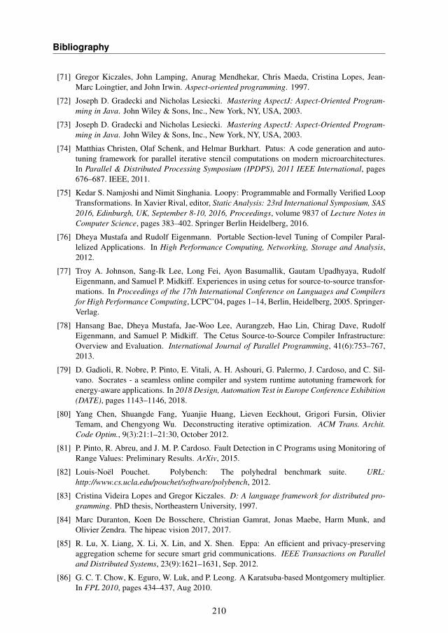
Bibliography
[71] Gregor Kiczales, John Lamping, Anurag Mendhekar, Chris Maeda, Cristina Lopes, Jean-Marc Loingtier, and John Irwin. Aspect-oriented programming. 1997.
[72] Joseph D. Gradecki and Nicholas Lesiecki. Mastering AspectJ: Aspect-Oriented Program-ming in Java. John Wiley & Sons, Inc., New York, NY, USA, 2003.
[73] Joseph D. Gradecki and Nicholas Lesiecki. Mastering AspectJ: Aspect-Oriented Program-ming in Java. John Wiley & Sons, Inc., New York, NY, USA, 2003.
[74] Matthias Christen, Olaf Schenk, and Helmar Burkhart. Patus: A code generation and auto-tuning framework for parallel iterative stencil computations on modern microarchitectures.In Parallel & Distributed Processing Symposium (IPDPS), 2011 IEEE International, pages676–687. IEEE, 2011.
[75] Kedar S. Namjoshi and Nimit Singhania. Loopy: Programmable and Formally Verified LoopTransformations. In Xavier Rival, editor, Static Analysis: 23rd International Symposium, SAS2016, Edinburgh, UK, September 8-10, 2016, Proceedings, volume 9837 of Lecture Notes inComputer Science, pages 383–402. Springer Berlin Heidelberg, 2016.
[76] Dheya Mustafa and Rudolf Eigenmann. Portable Section-level Tuning of Compiler Paral-lelized Applications. In High Performance Computing, Networking, Storage and Analysis,2012.
[77] Troy A. Johnson, Sang-Ik Lee, Long Fei, Ayon Basumallik, Gautam Upadhyaya, RudolfEigenmann, and Samuel P. Midkiff. Experiences in using cetus for source-to-source transfor-mations. In Proceedings of the 17th International Conference on Languages and Compilersfor High Performance Computing, LCPC’04, pages 1–14, Berlin, Heidelberg, 2005. Springer-Verlag.
[78] Hansang Bae, Dheya Mustafa, Jae-Woo Lee, Aurangzeb, Hao Lin, Chirag Dave, RudolfEigenmann, and Samuel P. Midkiff. The Cetus Source-to-Source Compiler Infrastructure:Overview and Evaluation. International Journal of Parallel Programming, 41(6):753–767,2013.
[79] D. Gadioli, R. Nobre, P. Pinto, E. Vitali, A. H. Ashouri, G. Palermo, J. Cardoso, and C. Sil-vano. Socrates - a seamless online compiler and system runtime autotuning framework forenergy-aware applications. In 2018 Design, Automation Test in Europe Conference Exhibition(DATE), pages 1143–1146, 2018.
[80] Yang Chen, Shuangde Fang, Yuanjie Huang, Lieven Eeckhout, Grigori Fursin, OlivierTemam, and Chengyong Wu. Deconstructing iterative optimization. ACM Trans. Archit.Code Optim., 9(3):21:1–21:30, October 2012.
[81] P. Pinto, R. Abreu, and J. M. P. Cardoso. Fault Detection in C Programs using Monitoring ofRange Values: Preliminary Results. ArXiv, 2015.
[82] Louis-Noël Pouchet. Polybench: The polyhedral benchmark suite. URL:http://www.cs.ucla.edu/pouchet/software/polybench, 2012.
[83] Cristina Videira Lopes and Gregor Kiczales. D: A language framework for distributed pro-gramming. PhD thesis, Northeastern University, 1997.
[84] Marc Duranton, Koen De Bosschere, Christian Gamrat, Jonas Maebe, Harm Munk, andOlivier Zendra. The hipeac vision 2017, 2017.
[85] R. Lu, X. Liang, X. Li, X. Lin, and X. Shen. Eppa: An efficient and privacy-preservingaggregation scheme for secure smart grid communications. IEEE Transactions on Paralleland Distributed Systems, 23(9):1621–1631, Sep. 2012.
[86] G. C. T. Chow, K. Eguro, W. Luk, and P. Leong. A Karatsuba-based Montgomery multiplier.In FPL 2010, pages 434–437, Aug 2010.
210
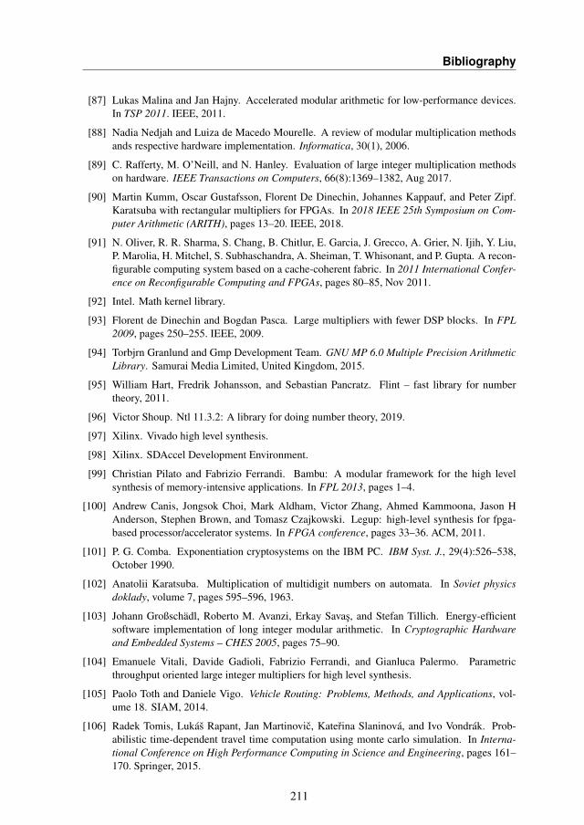
Bibliography
[87] Lukas Malina and Jan Hajny. Accelerated modular arithmetic for low-performance devices.In TSP 2011. IEEE, 2011.
[88] Nadia Nedjah and Luiza de Macedo Mourelle. A review of modular multiplication methodsands respective hardware implementation. Informatica, 30(1), 2006.
[89] C. Rafferty, M. O’Neill, and N. Hanley. Evaluation of large integer multiplication methodson hardware. IEEE Transactions on Computers, 66(8):1369–1382, Aug 2017.
[90] Martin Kumm, Oscar Gustafsson, Florent De Dinechin, Johannes Kappauf, and Peter Zipf.Karatsuba with rectangular multipliers for FPGAs. In 2018 IEEE 25th Symposium on Com-puter Arithmetic (ARITH), pages 13–20. IEEE, 2018.
[91] N. Oliver, R. R. Sharma, S. Chang, B. Chitlur, E. Garcia, J. Grecco, A. Grier, N. Ijih, Y. Liu,P. Marolia, H. Mitchel, S. Subhaschandra, A. Sheiman, T. Whisonant, and P. Gupta. A recon-figurable computing system based on a cache-coherent fabric. In 2011 International Confer-ence on Reconfigurable Computing and FPGAs, pages 80–85, Nov 2011.
[92] Intel. Math kernel library.
[93] Florent de Dinechin and Bogdan Pasca. Large multipliers with fewer DSP blocks. In FPL2009, pages 250–255. IEEE, 2009.
[94] Torbjrn Granlund and Gmp Development Team. GNU MP 6.0 Multiple Precision ArithmeticLibrary. Samurai Media Limited, United Kingdom, 2015.
[95] William Hart, Fredrik Johansson, and Sebastian Pancratz. Flint – fast library for numbertheory, 2011.
[96] Victor Shoup. Ntl 11.3.2: A library for doing number theory, 2019.
[97] Xilinx. Vivado high level synthesis.
[98] Xilinx. SDAccel Development Environment.
[99] Christian Pilato and Fabrizio Ferrandi. Bambu: A modular framework for the high levelsynthesis of memory-intensive applications. In FPL 2013, pages 1–4.
[100] Andrew Canis, Jongsok Choi, Mark Aldham, Victor Zhang, Ahmed Kammoona, Jason HAnderson, Stephen Brown, and Tomasz Czajkowski. Legup: high-level synthesis for fpga-based processor/accelerator systems. In FPGA conference, pages 33–36. ACM, 2011.
[101] P. G. Comba. Exponentiation cryptosystems on the IBM PC. IBM Syst. J., 29(4):526–538,October 1990.
[102] Anatolii Karatsuba. Multiplication of multidigit numbers on automata. In Soviet physicsdoklady, volume 7, pages 595–596, 1963.
[103] Johann Großschädl, Roberto M. Avanzi, Erkay Savas, and Stefan Tillich. Energy-efficientsoftware implementation of long integer modular arithmetic. In Cryptographic Hardwareand Embedded Systems – CHES 2005, pages 75–90.
[104] Emanuele Vitali, Davide Gadioli, Fabrizio Ferrandi, and Gianluca Palermo. Parametricthroughput oriented large integer multipliers for high level synthesis.
[105] Paolo Toth and Daniele Vigo. Vehicle Routing: Problems, Methods, and Applications, vol-ume 18. SIAM, 2014.
[106] Radek Tomis, Lukáš Rapant, Jan Martinovic, Katerina Slaninová, and Ivo Vondrák. Prob-abilistic time-dependent travel time computation using monte carlo simulation. In Interna-tional Conference on High Performance Computing in Science and Engineering, pages 161–170. Springer, 2015.
211
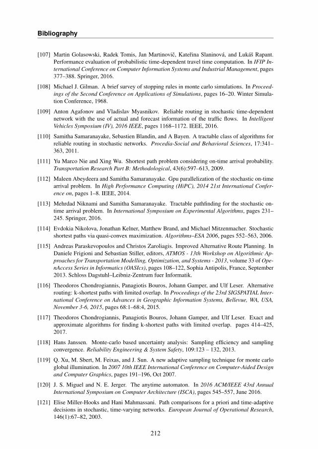
Bibliography
[107] Martin Golasowski, Radek Tomis, Jan Martinovic, Katerina Slaninová, and Lukáš Rapant.Performance evaluation of probabilistic time-dependent travel time computation. In IFIP In-ternational Conference on Computer Information Systems and Industrial Management, pages377–388. Springer, 2016.
[108] Michael J. Gilman. A brief survey of stopping rules in monte carlo simulations. In Proceed-ings of the Second Conference on Applications of Simulations, pages 16–20. Winter Simula-tion Conference, 1968.
[109] Anton Agafonov and Vladislav Myasnikov. Reliable routing in stochastic time-dependentnetwork with the use of actual and forecast information of the traffic flows. In IntelligentVehicles Symposium (IV), 2016 IEEE, pages 1168–1172. IEEE, 2016.
[110] Samitha Samaranayake, Sebastien Blandin, and A Bayen. A tractable class of algorithms forreliable routing in stochastic networks. Procedia-Social and Behavioral Sciences, 17:341–363, 2011.
[111] Yu Marco Nie and Xing Wu. Shortest path problem considering on-time arrival probability.Transportation Research Part B: Methodological, 43(6):597–613, 2009.
[112] Maleen Abeydeera and Samitha Samaranayake. Gpu parallelization of the stochastic on-timearrival problem. In High Performance Computing (HiPC), 2014 21st International Confer-ence on, pages 1–8. IEEE, 2014.
[113] Mehrdad Niknami and Samitha Samaranayake. Tractable pathfinding for the stochastic on-time arrival problem. In International Symposium on Experimental Algorithms, pages 231–245. Springer, 2016.
[114] Evdokia Nikolova, Jonathan Kelner, Matthew Brand, and Michael Mitzenmacher. Stochasticshortest paths via quasi-convex maximization. Algorithms–ESA 2006, pages 552–563, 2006.
[115] Andreas Paraskevopoulos and Christos Zaroliagis. Improved Alternative Route Planning. InDaniele Frigioni and Sebastian Stiller, editors, ATMOS - 13th Workshop on Algorithmic Ap-proaches for Transportation Modelling, Optimization, and Systems - 2013, volume 33 of Ope-nAccess Series in Informatics (OASIcs), pages 108–122, Sophia Antipolis, France, September2013. Schloss Dagstuhl–Leibniz-Zentrum fuer Informatik.
[116] Theodoros Chondrogiannis, Panagiotis Bouros, Johann Gamper, and Ulf Leser. Alternativerouting: k-shortest paths with limited overlap. In Proceedings of the 23rd SIGSPATIAL Inter-national Conference on Advances in Geographic Information Systems, Bellevue, WA, USA,November 3-6, 2015, pages 68:1–68:4, 2015.
[117] Theodoros Chondrogiannis, Panagiotis Bouros, Johann Gamper, and Ulf Leser. Exact andapproximate algorithms for finding k-shortest paths with limited overlap. pages 414–425,2017.
[118] Hans Janssen. Monte-carlo based uncertainty analysis: Sampling efficiency and samplingconvergence. Reliability Engineering & System Safety, 109:123 – 132, 2013.
[119] Q. Xu, M. Sbert, M. Feixas, and J. Sun. A new adaptive sampling technique for monte carloglobal illumination. In 2007 10th IEEE International Conference on Computer-Aided Designand Computer Graphics, pages 191–196, Oct 2007.
[120] J. S. Miguel and N. E. Jerger. The anytime automaton. In 2016 ACM/IEEE 43rd AnnualInternational Symposium on Computer Architecture (ISCA), pages 545–557, June 2016.
[121] Elise Miller-Hooks and Hani Mahmassani. Path comparisons for a priori and time-adaptivedecisions in stochastic, time-varying networks. European Journal of Operational Research,146(1):67–82, 2003.
212
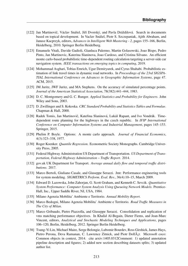
Bibliography
[122] Jan Martinovic, Václav Snášel, Jirí Dvorský, and Pavla Dráždilová. Search in documentsbased on topical development. In Vaclav Snášel, Piotr S. Szczepaniak, Ajith Abraham, andJanusz Kacprzyk, editors, Advances in Intelligent Web Mastering - 2, pages 155–166, Berlin,Heidelberg, 2010. Springer Berlin Heidelberg.
[123] Emanuele Vitali, Davide Gadioli, Gianluca Palermo, Martin Golasowski, Joao Bispo, PedroPinto, Jan Martinovic, Katerina Slaninova, Joao Cardoso, and Cristina Silvano. An efficientmonte carlo-based probabilistic time-dependent routing calculation targeting a server-side carnavigation system. IEEE transactions on emerging topics in computing, 2019.
[124] Mohammad Asghari, Tobias Emrich, Ugur Demiryurek, and Cyrus Shahabi. Probabilistic es-timation of link travel times in dynamic road networks. In Proceedings of the 23rd SIGSPA-TIAL International Conference on Advances in Geographic Information Systems, page 47.ACM, 2015.
[125] JM Juritz, JWF Juritz, and MA Stephens. On the accuracy of simulated percentage points.Journal of the American Statistical Association, 78(382):441–444, 1983.
[126] D. C. Montgomery and G. C. Runger. Applied Statistics and Probability for Engineers. JohnWiley and Sons, 2003.
[127] D. Zwillinger and S. Kokoska. CRC Standard Probability and Statistics Tables and Formulae.Chapman & Hall, 2000.
[128] Radek Tomis, Jan Martinovic, Katerina Slaninová, Lukáš Rapant, and Ivo Vondrák. Time-dependent route planning for the highways in the czech republic. In IFIP InternationalConference on Computer Information Systems and Industrial Management, pages 145–153.Springer, 2015.
[129] Phelim P. Boyle. Options: A monte carlo approach. Journal of Financial Economics,4(3):323–338, 1977.
[130] Roger Koenker. Quantile Regression. Econometric Society Monographs. Cambridge Univer-sity Press, 2005.
[131] Federal Highway Administration US Department of Transportation. US Department of Trans-portation, Federal Highway Administration – Traffic Report. 2014.
[132] gov.uk UK Department for Transport. Average annual daily flow and temporal traffic distri-butions. 2017.
[133] Marco Bertoli, Giuliano Casale, and Giuseppe Serazzi. Jmt: Performance engineering toolsfor system modeling. SIGMETRICS Perform. Eval. Rev., 36(4):10–15, March 2009.
[134] Edward D. Lazowska, John Zahorjan, G. Scott Graham, and Kenneth C. Sevcik. QuantitativeSystem Performance: Computer System Analysis Using Queueing Network Models. Prentice-Hall, Inc., Upper Saddle River, NJ, USA, 1984.
[135] Milano Agenzia Mobilita’ Ambiente e Territorio. Annual Mobility Report.
[136] Marco Bedogni, Milano Agenzia Mobilita’ Ambiente e Territorio. Road Traffic Measures inThe City of Milan.
[137] Marco Gribaudo, Pietro Piazzolla, and Giuseppe Serazzi. Consolidation and replication ofvms matching performance objectives. In Khalid Al-Begain, Dieter Fiems, and Jean-MarcVincent, editors, Analytical and Stochastic Modeling Techniques and Applications, pages106–120, Berlin, Heidelberg, 2012. Springer Berlin Heidelberg.
[138] Tsung-Yi Lin, Michael Maire, Serge Belongie, Lubomir Bourdev, Ross Girshick, James Hays,Pietro Perona, Deva Ramanan, C. Lawrence Zitnick, and Piotr Dollár. Microsoft coco:Common objects in context, 2014. cite arxiv:1405.0312Comment: 1) updated annotationpipeline description and figures; 2) added new section describing datasets splits; 3) updatedauthor list.
213
Bibliography
[139] Alex Krizhevsky, Ilya Sutskever, and Geoffrey E Hinton. Imagenet classification with deepconvolutional neural networks. Communications of the ACM, 60(6):84–90, 2017.
[140] Dario Amodei, Sundaram Ananthanarayanan, Rishita Anubhai, Jingliang Bai, Eric Batten-berg, Carl Case, Jared Casper, Bryan Catanzaro, Qiang Cheng, Guoliang Chen, et al. Deepspeech 2: End-to-end speech recognition in english and mandarin. In International confer-ence on machine learning, pages 173–182, 2016.
[141] Ross Girshick, Jeff Donahue, Trevor Darrell, and Jitendra Malik. Rich feature hierarchies foraccurate object detection and semantic segmentation. In Proceedings of the IEEE Conferenceon Computer Vision and Pattern Recognition (CVPR), June 2014.
[142] Olga Russakovsky, Jia Deng, Hao Su, Jonathan Krause, Sanjeev Satheesh, Sean Ma, ZhihengHuang, Andrej Karpathy, Aditya Khosla, Michael Bernstein, et al. Imagenet large scale visualrecognition challenge. International journal of computer vision, 115(3):211–252, 2015.
[143] Jonathan Huang, Vivek Rathod, Chen Sun, Menglong Zhu, Anoop Korattikara, Alireza Fathi,Ian Fischer, Zbigniew Wojna, Yang Song, Sergio Guadarrama, et al. Speed/accuracy trade-offs for modern convolutional object detectors. In Proceedings of the IEEE conference oncomputer vision and pattern recognition, pages 7310–7311, 2017.
[144] Ben Taylor, Vicent Sanz Marco, Willy Wolff, Yehia Elkhatib, and Zheng Wang. Adaptivedeep learning model selection on embedded systems. ACM SIGPLAN Notices, 53(6):31–43,2018.
[145] E. Park, D. Kim, S. Kim, Y. Kim, G. Kim, S. Yoon, and S. Yoo. Big/little deep neural net-work for ultra low power inference. In 2015 International Conference on Hardware/SoftwareCodesign and System Synthesis (CODES+ISSS), pages 124–132, 2015.
[146] Hokchhay Tann, Soheil Hashemi, and Sherief Reda. Flexible deep neural network processing.arXiv preprint arXiv:1801.07353, 2018.
[147] Mingxing Tan, Bo Chen, Ruoming Pang, Vijay Vasudevan, Mark Sandler, Andrew Howard,and Quoc V Le. Mnasnet: Platform-aware neural architecture search for mobile. In Proceed-ings of the IEEE Conference on Computer Vision and Pattern Recognition, pages 2820–2828,2019.
[148] Sicong Liu, Yingyan Lin, Zimu Zhou, Kaiming Nan, Hui Liu, and Junzhao Du. On-demanddeep model compression for mobile devices: A usage-driven model selection framework. InProceedings of the 16th Annual International Conference on Mobile Systems, Applications,and Services, MobiSys 2018, pages 389–400, New York, NY, USA, 2018. Association forComputing Machinery.
[149] A. Mazouz and C. P. Bridges. Multi-sensory cnn models for close proximity satellite opera-tions. In 2019 IEEE Aerospace Conference, pages 1–7, 2019.
[150] Emanuele Vitali and Anton Lokhmotov. omni benchmark-ing object detection. https://towardsdatascience.com/omni-benchmarking-object-detection-b390cc4114cd. Accessed: 2021-02-22.
[151] Andreas Geiger, Philip Lenz, and Raquel Urtasun. Are we ready for autonomous driving?the kitti vision benchmark suite. In Conference on Computer Vision and Pattern Recognition(CVPR), 2012.
[152] Mahmoud Hassaballah, Aly Amin Abdelmgeid, and Hammam A Alshazly. Image featuresdetection, description and matching. In Image Feature Detectors and Descriptors, pages11–45. Springer, 2016.
[153] OpenCV. Open source computer vision library, 2015.
214
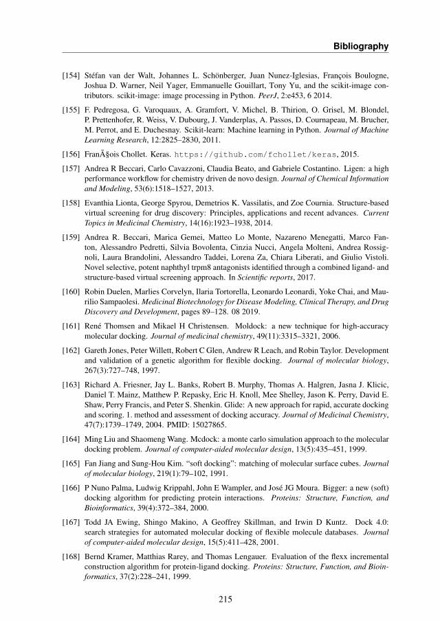
Bibliography
[154] Stéfan van der Walt, Johannes L. Schönberger, Juan Nunez-Iglesias, François Boulogne,Joshua D. Warner, Neil Yager, Emmanuelle Gouillart, Tony Yu, and the scikit-image con-tributors. scikit-image: image processing in Python. PeerJ, 2:e453, 6 2014.
[155] F. Pedregosa, G. Varoquaux, A. Gramfort, V. Michel, B. Thirion, O. Grisel, M. Blondel,P. Prettenhofer, R. Weiss, V. Dubourg, J. Vanderplas, A. Passos, D. Cournapeau, M. Brucher,M. Perrot, and E. Duchesnay. Scikit-learn: Machine learning in Python. Journal of MachineLearning Research, 12:2825–2830, 2011.
[156] François Chollet. Keras. https://github.com/fchollet/keras, 2015.
[157] Andrea R Beccari, Carlo Cavazzoni, Claudia Beato, and Gabriele Costantino. Ligen: a highperformance workflow for chemistry driven de novo design. Journal of Chemical Informationand Modeling, 53(6):1518–1527, 2013.
[158] Evanthia Lionta, George Spyrou, Demetrios K. Vassilatis, and Zoe Cournia. Structure-basedvirtual screening for drug discovery: Principles, applications and recent advances. CurrentTopics in Medicinal Chemistry, 14(16):1923–1938, 2014.
[159] Andrea R. Beccari, Marica Gemei, Matteo Lo Monte, Nazareno Menegatti, Marco Fan-ton, Alessandro Pedretti, Silvia Bovolenta, Cinzia Nucci, Angela Molteni, Andrea Rossig-noli, Laura Brandolini, Alessandro Taddei, Lorena Za, Chiara Liberati, and Giulio Vistoli.Novel selective, potent naphthyl trpm8 antagonists identified through a combined ligand- andstructure-based virtual screening approach. In Scientific reports, 2017.
[160] Robin Duelen, Marlies Corvelyn, Ilaria Tortorella, Leonardo Leonardi, Yoke Chai, and Mau-rilio Sampaolesi. Medicinal Biotechnology for Disease Modeling, Clinical Therapy, and DrugDiscovery and Development, pages 89–128. 08 2019.
[161] René Thomsen and Mikael H Christensen. Moldock: a new technique for high-accuracymolecular docking. Journal of medicinal chemistry, 49(11):3315–3321, 2006.
[162] Gareth Jones, Peter Willett, Robert C Glen, Andrew R Leach, and Robin Taylor. Developmentand validation of a genetic algorithm for flexible docking. Journal of molecular biology,267(3):727–748, 1997.
[163] Richard A. Friesner, Jay L. Banks, Robert B. Murphy, Thomas A. Halgren, Jasna J. Klicic,Daniel T. Mainz, Matthew P. Repasky, Eric H. Knoll, Mee Shelley, Jason K. Perry, David E.Shaw, Perry Francis, and Peter S. Shenkin. Glide: A new approach for rapid, accurate dockingand scoring. 1. method and assessment of docking accuracy. Journal of Medicinal Chemistry,47(7):1739–1749, 2004. PMID: 15027865.
[164] Ming Liu and Shaomeng Wang. Mcdock: a monte carlo simulation approach to the moleculardocking problem. Journal of computer-aided molecular design, 13(5):435–451, 1999.
[165] Fan Jiang and Sung-Hou Kim. “soft docking”: matching of molecular surface cubes. Journalof molecular biology, 219(1):79–102, 1991.
[166] P Nuno Palma, Ludwig Krippahl, John E Wampler, and José JG Moura. Bigger: a new (soft)docking algorithm for predicting protein interactions. Proteins: Structure, Function, andBioinformatics, 39(4):372–384, 2000.
[167] Todd JA Ewing, Shingo Makino, A Geoffrey Skillman, and Irwin D Kuntz. Dock 4.0:search strategies for automated molecular docking of flexible molecule databases. Journalof computer-aided molecular design, 15(5):411–428, 2001.
[168] Bernd Kramer, Matthias Rarey, and Thomas Lengauer. Evaluation of the flexx incrementalconstruction algorithm for protein-ligand docking. Proteins: Structure, Function, and Bioin-formatics, 37(2):228–241, 1999.
215
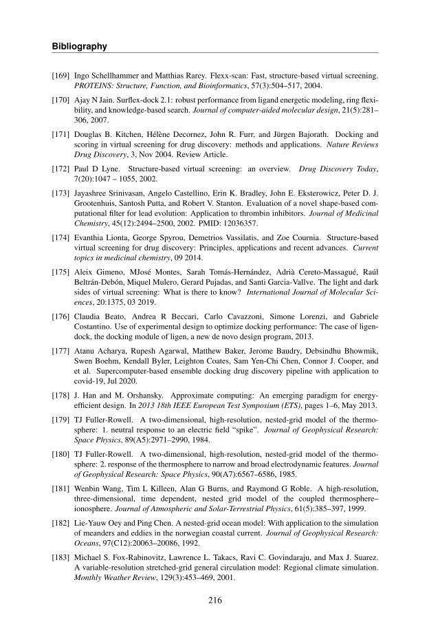
Bibliography
[169] Ingo Schellhammer and Matthias Rarey. Flexx-scan: Fast, structure-based virtual screening.PROTEINS: Structure, Function, and Bioinformatics, 57(3):504–517, 2004.
[170] Ajay N Jain. Surflex-dock 2.1: robust performance from ligand energetic modeling, ring flexi-bility, and knowledge-based search. Journal of computer-aided molecular design, 21(5):281–306, 2007.
[171] Douglas B. Kitchen, Hélène Decornez, John R. Furr, and Jürgen Bajorath. Docking andscoring in virtual screening for drug discovery: methods and applications. Nature ReviewsDrug Discovery, 3, Nov 2004. Review Article.
[172] Paul D Lyne. Structure-based virtual screening: an overview. Drug Discovery Today,7(20):1047 – 1055, 2002.
[173] Jayashree Srinivasan, Angelo Castellino, Erin K. Bradley, John E. Eksterowicz, Peter D. J.Grootenhuis, Santosh Putta, and Robert V. Stanton. Evaluation of a novel shape-based com-putational filter for lead evolution: Application to thrombin inhibitors. Journal of MedicinalChemistry, 45(12):2494–2500, 2002. PMID: 12036357.
[174] Evanthia Lionta, George Spyrou, Demetrios Vassilatis, and Zoe Cournia. Structure-basedvirtual screening for drug discovery: Principles, applications and recent advances. Currenttopics in medicinal chemistry, 09 2014.
[175] Aleix Gimeno, MJosé Montes, Sarah Tomás-Hernández, Adrià Cereto-Massagué, RaúlBeltrán-Debón, Miquel Mulero, Gerard Pujadas, and Santi Garcia-Vallve. The light and darksides of virtual screening: What is there to know? International Journal of Molecular Sci-ences, 20:1375, 03 2019.
[176] Claudia Beato, Andrea R Beccari, Carlo Cavazzoni, Simone Lorenzi, and GabrieleCostantino. Use of experimental design to optimize docking performance: The case of ligen-dock, the docking module of ligen, a new de novo design program, 2013.
[177] Atanu Acharya, Rupesh Agarwal, Matthew Baker, Jerome Baudry, Debsindhu Bhowmik,Swen Boehm, Kendall Byler, Leighton Coates, Sam Yen-Chi Chen, Connor J. Cooper, andet al. Supercomputer-based ensemble docking drug discovery pipeline with application tocovid-19, Jul 2020.
[178] J. Han and M. Orshansky. Approximate computing: An emerging paradigm for energy-efficient design. In 2013 18th IEEE European Test Symposium (ETS), pages 1–6, May 2013.
[179] TJ Fuller-Rowell. A two-dimensional, high-resolution, nested-grid model of the thermo-sphere: 1. neutral response to an electric field “spike”. Journal of Geophysical Research:Space Physics, 89(A5):2971–2990, 1984.
[180] TJ Fuller-Rowell. A two-dimensional, high-resolution, nested-grid model of the thermo-sphere: 2. response of the thermosphere to narrow and broad electrodynamic features. Journalof Geophysical Research: Space Physics, 90(A7):6567–6586, 1985.
[181] Wenbin Wang, Tim L Killeen, Alan G Burns, and Raymond G Roble. A high-resolution,three-dimensional, time dependent, nested grid model of the coupled thermosphere–ionosphere. Journal of Atmospheric and Solar-Terrestrial Physics, 61(5):385–397, 1999.
[182] Lie-Yauw Oey and Ping Chen. A nested-grid ocean model: With application to the simulationof meanders and eddies in the norwegian coastal current. Journal of Geophysical Research:Oceans, 97(C12):20063–20086, 1992.
[183] Michael S. Fox-Rabinovitz, Lawrence L. Takacs, Ravi C. Govindaraju, and Max J. Suarez.A variable-resolution stretched-grid general circulation model: Regional climate simulation.Monthly Weather Review, 129(3):453–469, 2001.
216
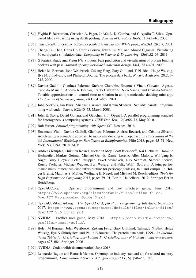
Bibliography
[184] Fábio F. Bernardon, Christian A. Pagot, João L. D. Comba, and Cláudio T. Silva. Gpu-based tiled ray casting using depth peeling. Journal of Graphics Tools, 11(4):1–16, 2006.
[185] Cass Everitt. Interactive order-independent transparency. White paper, nVIDIA, 2(6):7, 2001.
[186] Cheng-Kai Chen, Chris Ho, Carlos Correa, Kwan-Liu Ma, and Ahmed Elgamal. Visualizing3d earthquake simulation data. Computing in Science & Engineering, 13(6):52–63, 2011.
[187] G Patrick Brady and Pieter FW Stouten. Fast prediction and visualization of protein bindingpockets with pass. Journal of computer-aided molecular design, 14(4):383–401, 2000.
[188] Helen M. Berman, John Westbrook, Zukang Feng, Gary Gilliland, T. N. Bhat, Helge Weissig,Ilya N. Shindyalov, and Philip E. Bourne. The protein data bank. Nucleic Acids Res, 28:235–242, 2000.
[189] Davide Gadioli, Gianluca Palermo, Stefano Cherubin, Emanuele Vitali, Giovanni Agosta,Candida Manelfi, Andrea R Beccari, Carlo Cavazzoni, Nico Sanna, and Cristina Silvano.Tunable approximations to control time-to-solution in an hpc molecular docking mini-app.The Journal of Supercomputing, 77(1):841–869, 2021.
[190] John Nickolls, Ian Buck, Michael Garland, and Kevin Skadron. Scalable parallel program-ming with cuda. Queue, 6(2):40–53, March 2008.
[191] John E. Stone, David Gohara, and Guochun Shi. Opencl: A parallel programming standardfor heterogeneous computing systems. IEEE Des. Test, 12(3):66–73, May 2010.
[192] Rob Farber. Parallel programming with OpenACC. Newnes, 2016.
[193] Emanuele Vitali, Davide Gadioli, Gianluca Palermo, Andrea Beccari, and Cristina Silvano.Accelerating a geometric approach to molecular docking with openacc. In Proceedings of the6th International Workshop on Parallelism in Bioinformatics, PBio 2018, pages 45–51, NewYork, NY, USA, 2018. ACM.
[194] Andreas Knüpfer, Christian Rössel, Dieter an Mey, Scott Biersdorff, Kai Diethelm, DominicEschweiler, Markus Geimer, Michael Gerndt, Daniel Lorenz, Allen Malony, Wolfgang E.Nagel, Yury Oleynik, Peter Philippen, Pavel Saviankou, Dirk Schmidl, Sameer Shende,Ronny Tschüter, Michael Wagner, Bert Wesarg, and Felix Wolf. Score-p: A joint perfor-mance measurement run-time infrastructure for periscope,scalasca, tau, and vampir. In Hol-ger Brunst, Matthias S. Müller, Wolfgang E. Nagel, and Michael M. Resch, editors, Tools forHigh Performance Computing 2011, pages 79–91, Berlin, Heidelberg, 2012. Springer BerlinHeidelberg.
[195] OpenACC.org. Openacc programming and best practices guide, June 2015.https://www.openacc.org/sites/default/files/inline-files/OpenACC_Programming_Guide_0.pdf.
[196] OpenACC-Standard.org. The OpenACC Application Programming Interface, November2017. https://www.openacc.org/sites/default/files/inline-files/OpenACC.2.6.final.pdf.
[197] NVIDIA. Profiler user guide, May 2018. https://docs.nvidia.com/cuda/profiler-users-guide/.
[198] Helen M Berman, John Westbrook, Zukang Feng, Gary Gilliland, Talapady N Bhat, HelgeWeissig, Ilya N Shindyalov, and Philip E Bourne. The protein data bank, 1999–. In Interna-tional Tables for Crystallography Volume F: Crystallography of biological macromolecules,pages 675–684. Springer, 2006.
[199] NVIDIA. Cuda toolkit documentation, June 2018.
[200] Leonardo Dagum and Ramesh Menon. Openmp: an industry standard api for shared-memoryprogramming. Computational Science & Engineering, IEEE, 5(1):46–55, 1998.
217
Bibliography
[201] S. Sawadsitang, J. Lin, S. See, F. Bodin, and S. Matsuoka. Understanding performance porta-bility of openacc for supercomputers. In 2015 IEEE International Parallel and DistributedProcessing Symposium Workshop, pages 699–707, May 2015.
[202] Yonghong Yan, Jiawen Liu, Kirk W. Cameron, and Mariam Umar. Homp: Automated distri-bution of parallel loops and data in highly parallel accelerator-based systems. pages 788–798,05 2017.
[203] Yonghong Yan, Pei-Hung Lin, Chunhua Liao, Bronis R. de Supinski, and Daniel J. Quin-lan. Supporting multiple accelerators in high-level programming models. pages 170–180, 022015.
[204] Rengan Xu, Xiaonan Tian, Sunita Chandrasekaran, and Barbara Chapman. Multi-gpu sup-port on single node using directive-based programming model. Sci. Program., 2015:3:3–3:3,January 2016.
[205] Stefano Markidis, Jing Gong, Michael Schliephake, Erwin Laure, Alistair Hart, David Henty,Katherine Heisey, and Paul Fischer. Openacc acceleration of the nek5000 spectral elementcode. The International Journal of High Performance Computing Applications, 29(3):311–319, 2015.
[206] Rengan Xu, Sunita Chandrasekaran, and Barbara Chapman. Exploring programming multi-gpus using openmp and openacc-based hybrid model. 05 2013.
[207] Emanuele Vitali, Davide Gadioli, Gianluca Palermo, Andrea Beccari, Carlo Cavazzoni, andCristina Silvano. Exploiting openmp and openacc to accelerate a geometric approach tomolecular docking in heterogeneous hpc nodes. The Journal of Supercomputing, 75(7):3374–3396, 2019.
[208] Gianluca Palermo, Davide Gadioli, Emanuele Vitali, Cristina Silvano, Federico Ficarelli,Chiara Latini, Andrea R Beccari, and Candida Manelfi. Exscalate4cov: Towards an exascale-ready docking platform targeting urgent computing. EuroHPC Week, 2021.
[209] Seyyed Reza Miri Rostami and Mohsen Ghaffari-Miab. Finite difference generated transientpotentials of open-layered media by parallel computing using openmp, mpi, openacc, andcuda. IEEE Transactions on Antennas and Propagation, 67(10):6541–6550, 2019.
[210] Gabriell Alves de Araujo, Dalvan Griebler, Marco Danelutto, and Luiz Gustavo Fernan-des. Efficient nas parallel benchmark kernels with cuda. In 2020 28th Euromicro Inter-national Conference on Parallel, Distributed and Network-Based Processing (PDP), pages9–16. IEEE, 2020.
[211] M Harris and K Perelygin. Cooperative groups: Flexible cuda thread programming, 2017.
218
Related Documents