A Holistic Approach to Multi-Scale, Coupled Modeling of ...

A Holistic Approach to Multi-Scale, Coupled Modeling of Hydrologic

Processes, Flow Dynamics, Erosion, and Sediment Transport

by

Jongho Kim

A dissertation submitted in partial fulfillment

of the requirements for the degree of

Doctor of Philosophy

(Civil Engineering)

in the University of Michigan

2013

Doctoral Committee:

Assistant Professor Valeriy Y. Ivanov, Chair

Assistant Professor Mark G. Flanner

Professor Nikolaos D. Katopodes

Professor Steve J. Wright

© Jongho Kim 2013

ii

DEDICATION

With great pleasure, I dedicate this to my wife, Eun Go.

iii

ACKNOWLEDGEMENTS

Over the last four and half years as a graduate student, this dissertation work has been

supported by the Graham Environmental Sustainability Institute at the University of Michigan

through the grant, the Rackham International Student Fellowship at the University of Michigan,

the Graduate Fellowship of the Department of Civil and Environmental Engineering at the

University of Michigan, and the NSF Grant EAR 1151443 .

The first unutterable appreciation is devoted to my advisor, Prof. Valeriy Y. Ivanov who

truly deserves to be admirable and support me throughout this long journey by offering me

motivation and encouragement. He always struggles with me every time we met challenging

problems, provides relevant and in-depth advice and guidance about complicated issues, and

motivates me to investigate many unresolved curious problems scattered in an interdisciplinary

area and to make a progress toward the higher scientific goal and vision. Other than the academic

assistances, he sincerely expresses encouragement rather than disappointment with a generous,

thoughtful, nice attitude when I am in a state of chaos and thus insufficiency of progress.

I am also very appreciative of their invaluable advice from my Ph.D. Committee

members: Prof. Nikolaos D. Katopodes, Prof. Steve J. Wright, and Prof. Mark G. Flanner. In

particular, I am very grateful to Dr. Katopodes for his organized remark and clear explanation on

research of flow dynamics; to Dr. Wright for his sharp opinion and insight coming out of his

iv

long-term experience on research of sediment transport; and to Dr. Flanner for his unforeseen

angles of view on research I have never considered.

Successful and satisfactory journey of dissertation cannot be attained without their helps.

I would like to thank to Dr. Brett Sanders for his help with the overland flow code and for

sharing his experience for the numerical difficulties; to Dr. D.S.L. Lawrence for her help with

experimental data used for verifying the upscaled regression equation developed in vegetated

area; and to my Italian friend, Dr. Simone Fatichi for sharing his wisdom in stochastic

downscaling to project future climate conditions. Furthermore, I would like to thank to all of the

other members in environmental water resources group including Prof. Aline Cotel and my

colleagues and friends, Antonio Francipane, April Warnock, Lingli He, Sara Rimer, Jenahvive

Morgan, Chase Dwelle, Frank Sedlar, and TaoTao for sharing their expertise and friendship.

Thanks for having a wonderful Ann Arbor life together to my Korean brothers: Sukhoon Pyo,

Seungjun Ahn, Joon-Oh Seo, Jun-Hyuk Kwon, and Hyon-Sohk Ohm.

To the greatest extent, this dissertation is devoted to my parents, Ilkyun Kim and Duckja

Im who always trust me every time I need to decide and express their unconditional love toward

us; and to my sister and brother, Eunja Kim and Hyun-Chul Kim who have been of great role in

our family to the part that I should do while I leave. Thank you very much.

Lastly, none of any conventional words can describe my love and gratitude to my wife,

Eun Go. The satisfactory completion of doctoral program cannot be attained without her

sacrifices and support. Her optimistic, pleasurable characteristics make me relieve any stress, and

enable to refresh myself to continue to work. Although any earthly deeds cannot compensate her

support, I will promise to keep me appreciate and remember it for the rest of my life.

v

TABLE OF CONTENTS

DEDICATION ................................................................................................................................ ii

ACKNOWLEDGEMENTS ........................................................................................................... iii

LIST OF TABLES .......................................................................................................................... x

LIST OF FIGURES ...................................................................................................................... xii

LIST OF APPENDICES .............................................................................................................. xxi

ABSTRACT ................................................................................................................................ xxii

CHAPTER

I. Introduction ............................................................................................................................... 1

1.1 Motivation of a holistic, multi-scale, coupled approach .................................................. 1

1.1.1 Climate change and human activity in watershed systems ....................................... 1

1.1.2 Significance and challenges of a multi-scale coupled approach ............................... 2

1.1.3 Characteristics of watershed systems: connectivity and non-linearity ..................... 4

1.1.4 The need for a holistic, multi-scale, coupled model ................................................. 5

1.2 Research scope ................................................................................................................. 6

II. Coupled modeling of hydrologic and hydrodynamic processes including overland and

channel flow: “tRIBS-OFM” ............................................................................................... 10

2.1 Introduction .................................................................................................................... 10

2.2 Description of the coupled model .................................................................................. 14

2.2.1 Model heritage: tRIBS ............................................................................................ 14

2.2.2 Model heritage: OFM ............................................................................................. 19

2.2.3 OFM modification .................................................................................................. 19

2.2.4 Information exchange between the hydrologic and hydrodynamic models ........... 23

vi

2.3 OFM verification ............................................................................................................ 26

2.3.1 One dimensional flow problem over mild-sloped plane ......................................... 26

2.3.2 One dimensional flow over steeply sloped plane ................................................... 28

2.3.3 Two dimensional flow problem in V-shaped catchment domain ........................... 29

2.3.4 A hydraulic jump problem for steep-to-mild slope transition ................................ 39

2.4 Model application ........................................................................................................... 41

2.4.1 Model application to a synthetic watershed ............................................................ 41

2.4.2 Model application to a natural watershed ............................................................... 46

2.4.2.1 A description of the Peacheater Creek watershed....................................... 46

2.4.2.2 Calibration of channel and hillslope routing parameters ............................ 48

2.4.2.3 Soil parameter calibration ........................................................................... 49

2.4.2.4 Parameterization of the hydrodynamic routing model................................ 51

2.4.2.5 Simulation results........................................................................................ 53

2.4.2.6 Hydrology-hydrodynamics coupling .......................................................... 58

2.5 Conclusions .................................................................................................................... 62

III. Hairsine-Rose erosion equations coupled with hydrological processes and overland flow

at watershed scale: “tRIBS-OFM-HRM” ......................................................................... 65

3.1 Introduction .................................................................................................................... 65

3.2 Governing equations ...................................................................................................... 70

3.3 Numerical model ............................................................................................................ 76

3.4 Model verification .......................................................................................................... 83

3.4.1 Rainfall-induced erosion ......................................................................................... 83

3.4.2 Overland flow-induced erosion............................................................................... 88

3.4.3 Lucky Hills watershed ............................................................................................ 91

3.4.3.1. Lucky Hills watershed and its numerical representation ........................... 91

3.4.3.2. Model calibration and confirmation........................................................... 97

3.4.3.3. Spatial characteristics of flow and erosion processes .............................. 104

3.4.3.4. Size-dependent characteristics and spatial variability of concentration .. 107

3.4.3.5. North- and south-facing characteristics of watershed system .................. 110

3.5 Summary ...................................................................................................................... 113

vii

IV. Hydraulic resistance to overland flow on surfaces with partially submerged

vegetation ............................................................................................................................ 116

4.1 Introduction .................................................................................................................. 116

4.2 Model suitability and simulation setup ........................................................................ 121

4.2.1 Model suitability ................................................................................................... 121

4.2.2 Simulation setup.................................................................................................... 122

4.3 Methods for determining a representative value of resistance coefficient ................... 125

4.3.1 Equivalent Roughness Surface ............................................................................. 126

4.3.2 Equivalent Friction Slope ..................................................................................... 127

4.4 Simulation results ......................................................................................................... 129

4.4.1 Overall characterization of flow variables ............................................................ 129

4.4.2 Results for the method of Equivalent Roughness Surface .................................... 133

4.4.3 Results for the method of Equivalent Friction Slope ............................................ 137

4.4.4 Predictive equations for nt ..................................................................................... 140

4.4.5 Verification of the regression equation ................................................................. 143

4.4.6 Comparison of results with previous studies ........................................................ 145

4.5 Discussion .................................................................................................................... 151

4.5.1 Effects of vegetation cover fraction ...................................................................... 151

4.5.2 Effects of bed slope ............................................................................................... 155

4.5.3 Effects of inflow rate ............................................................................................ 159

4.5.4 Effects of bed surface roughness condition .......................................................... 160

4.5.5 Relationship between flow depth or velocity and the Manning coefficient ......... 163

4.5.6 Validity of performance skill ................................................................................ 164

4.6 Conclusions .................................................................................................................. 165

V. On the non-uniqueness of sediment yield: effects of initialization and surface shield .. 167

5.1 Introduction .................................................................................................................. 167

5.2 Model appropriateness and simulation design ............................................................. 171

5.2.1 Model appropriateness .......................................................................................... 171

5.2.2 Modeling erosion processes .................................................................................. 171

viii

5.2.3 Simulation setup.................................................................................................... 174

5.2.3.1 Domain and modeling configuration ........................................................ 174

5.2.3.2 Rainfall forcing ......................................................................................... 175

5.2.3.3 Soil characterization.................................................................................. 178

5.2.3.4 Model parameterization ............................................................................ 179

5.3 Simulation results ......................................................................................................... 180

5.3.1 Case 1 .................................................................................................................... 181

5.3.2 Case 2 .................................................................................................................... 182

5.3.3 Case 3 .................................................................................................................... 182

5.3.4 Cases 4 and 5 ........................................................................................................ 183

5.4 Discussion .................................................................................................................... 188

5.4.1 Variations of sediment yield for the same flow volume ....................................... 188

5.4.2 Initialization effects on the non-uniqueness of sediment yield ............................. 194

5.4.3 Patterns of evolution of sediment yield and critical time scales ........................... 197

5.4.4 Patterns of temporal evolution specific to particle sizes ....................................... 203

5.5 Conclusions .................................................................................................................. 207

VI. Research summary and perspectives for future studies ................................................. 210

6.1 Summary of research .................................................................................................... 210

6.2 Critical assumptions and limitations of the research .................................................... 215

6.3 Uncertainties in the multi-scale modeling .................................................................... 219

6.3.1 Verification of the coupled model ........................................................................ 219

6.3.2 Calibration of the coupled model .......................................................................... 221

6.4 An feasibility study of soil loss assessment ................................................................. 222

6.4.1 USLE database and rainfall disaggregation .......................................................... 224

6.4.2 Numerical representation and results .................................................................... 228

6.5 Future studies ............................................................................................................... 230

6.5.1 Eco-hydrologic-hydraulic-morphologic modeling and their interactions............. 230

6.5.2 Future assessment studies with uncertainty analyses under climate change ........ 231

6.5.3 A longer time simulation with a parallel mode ..................................................... 233

ix

APPENDICES ............................................................................................................................ 234

NOTATION ................................................................................................................................ 244

BIBLIOGRAPHY ....................................................................................................................... 248

x

LIST OF TABLES

Table 2.1: A summary of processes considered in the hydrologic model tRIBS. ........................ 17

Table 2.2: The soil hydraulic and thermal parameters used in calibration for

Peacheater Creek ................................................................................................................... 18

Table 2.3: The Manning roughness coefficients [s/m1/3

] used in calibration for

Peacheater Creek ................................................................................................................... 52

Table 2.4: The error indices of the simulation results for Peacheater Creek. ............................... 53

Table 3.1: Hydraulics-based erosion and sediment transport models ........................................... 67

Table 3.2: Simulation conditions and parameters for Aridsol (Solonchak) after Sander

et al. [1996] ............................................................................................................................ 84

Table 3.3: A summary of observed rainfall, runoff, and sediment for events used in

simulations for the Lucky Hills watershed. Rainfall was measured at “Gage 83”.

Runoff and sediment were measured at flume “FL103” ....................................................... 97

Table 3.4: Parameters used to represent hydrologic, hydraulic, and sediment erosion-

transport dynamics of the Lucky Hills watershed. The letter “C” refers to the

parameters whose values were calibrated; “L” refers to the parameters whose

values were inferred from literature ...................................................................................... 99

Table 4.1: The mean values and the correlation coefficients for the entire domain for

the cases of both Vf = 0 and Vf = 0.3. Only a subset of cases with small, medium,

and high friction slopes were selected for the case of Vf = 0.3. (Corr=Correlation) .......... 132

Table 4.2: A summary of the simulation cases. Each characteristic was permutated

with all other variables. The total number of simulations is 324 ......................................... 134

Table 4.3: A summary of simulation cases used in comparisons with the equivalent

roughness surface method. The total number of simulations is 144 .................................... 135

Table 4.4: A summary of simulation cases with high inflow rates. The total number of

simulations is 30 .................................................................................................................. 143

Table 4.5: A summary of simulation cases used for the verification of the regression

equation. The total number of simulations is 12 .................................................................. 144

xi

Table 4.6: A summary of experimental studies used in the comparison. Notation “lab”

is used for data obtained in laboratory conditions; “field” is used to denote field

studies .................................................................................................................................. 146

Table 4.7 The means and the standard deviations of the difference between the

upscaled and base Manning‟s coefficient . Results for all simulations are

presented. (SD=Standard deviation) .................................................................................... 153

Table 5.1: A summary of five principal simulation cases. The total number of

simulations is 95 .................................................................................................................. 177

Table 5.2: The model parameters used to represent hydrologic, hydraulic, and

sediment erosion-transport dynamics .................................................................................. 180

Table 5.3: Variations of sediment yield VSY [%] for all Cases shown in Figure 5.7 with

respect to the same volume of rainfall corresponding to either the second event

(Cases 1, 2, and 3 in sub-plots (a)-(c)), the entire single event (Cases 3 and 4, sub-

plots (d)-(e)), or hourly volumes (Case 5, sub-plot (f)).The last two columns

represent variations illustrated in Figure 5.7-(d) ................................................................. 192

Table 6.1: A summary of USLE field locations and WebMET database climate

stations used for rainfall disaggregation. The “Lat.” and “Lon.” denote the latitude

of longitude of the USLE locations; the “mi” denotes the distances in miles

between original locations and WebMET meteorological stations. The last column

reports the period for which the hourly time series of precipitation in WebMET

stations are available. ........................................................................................................... 225

Table 6.2: Parameters used to represent hydrologic, hydraulic, and sediment erosion-

transport dynamics for the location of Watkinsville, GA. The letter “C” refers to

the parameters whose values were calibrated; “L” refers to the parameters whose

values were inferred from literature. ................................................................................... 229

xii

LIST OF FIGURES

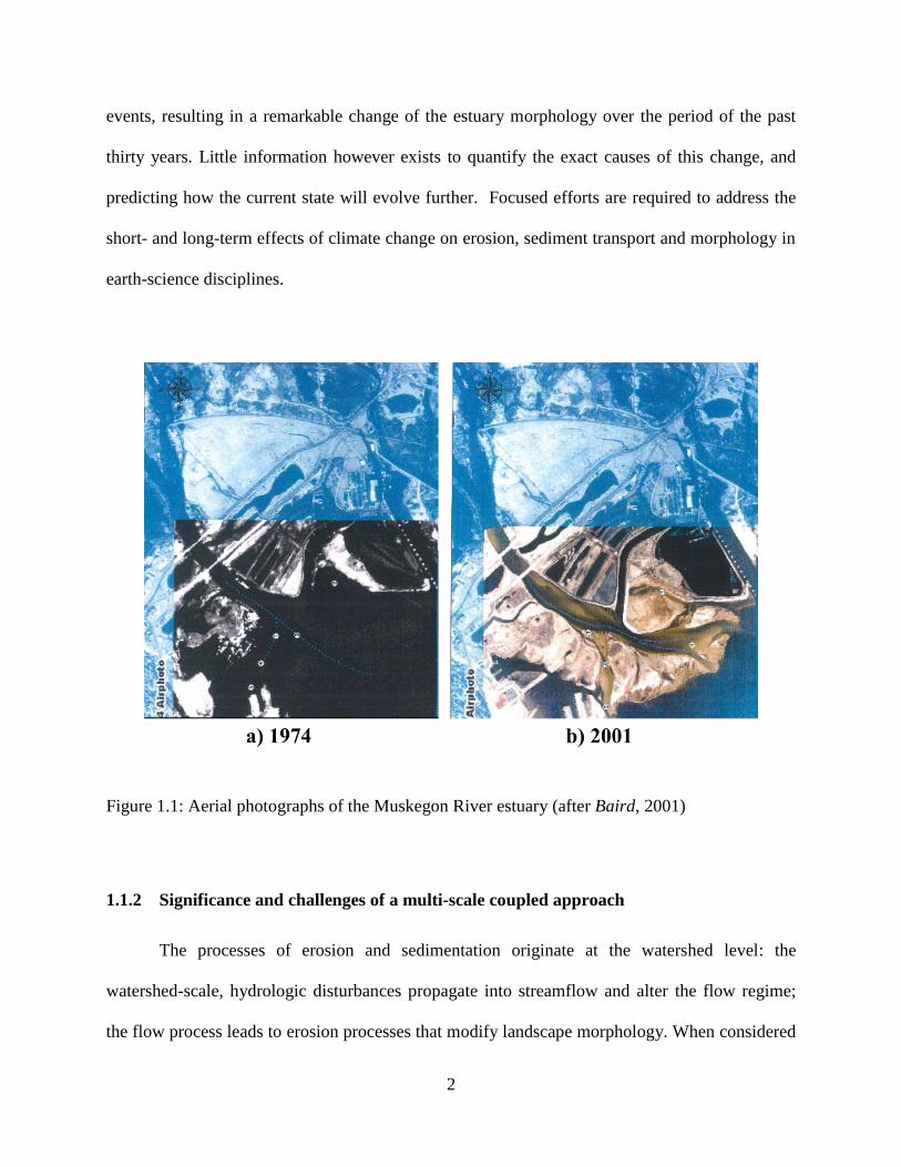
Figure 1.1: Aerial photographs of the Muskegon River estuary (after Baird, 2001)...................... 2

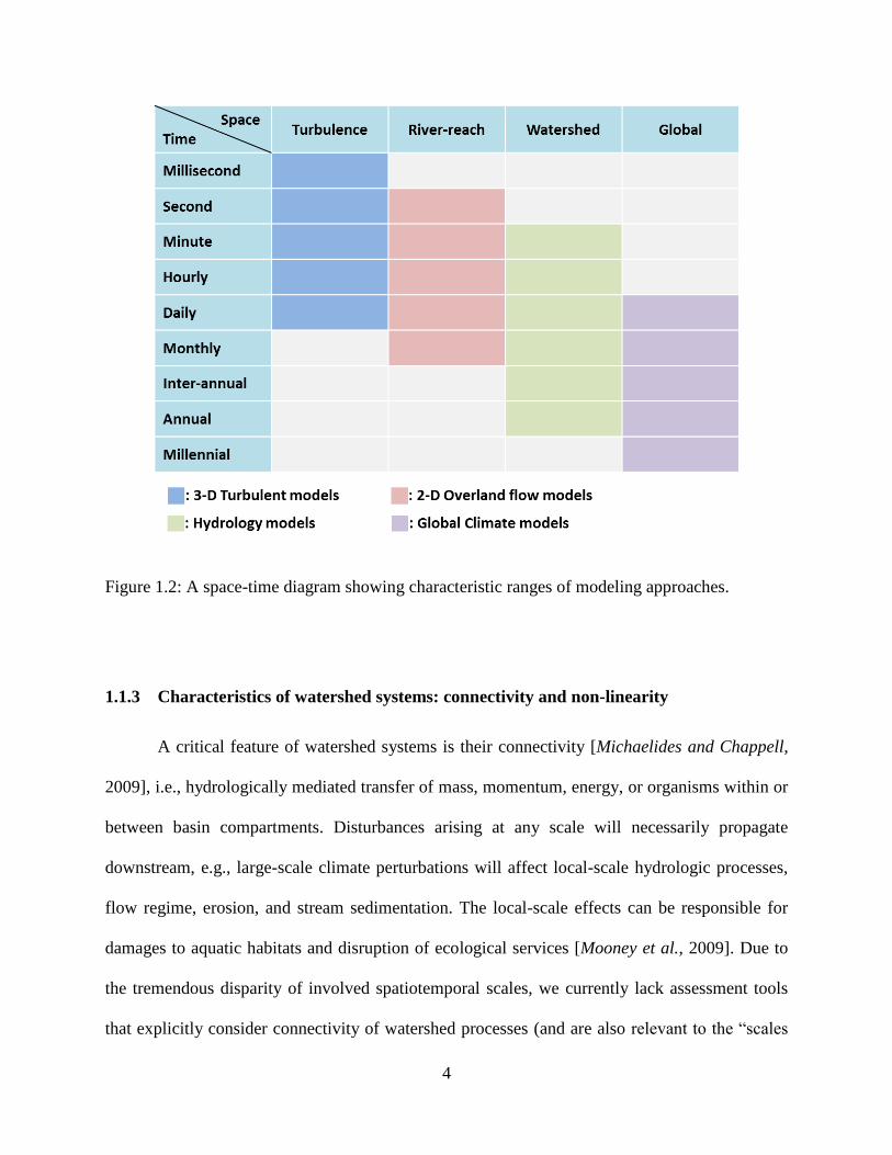
Figure 1.2: A space-time diagram showing characteristic ranges of modeling

approaches. .............................................................................................................................. 4

Figure 2.1: Flow regimes near the wet and dry boundary on a sloped bed: (a) the

quiescent flow regime characteristic of hydraulic applications, such as flooding

and wave runup; (b) an incorrect representation of flow regime using the concept

(a) for hydrological applications; and (c) the sheet flow representation of a flow

regime for hydrological applications with low runoff on a steeply sloped bed. .................... 21

Figure 2.2: A schematic diagram of the mapping procedure. ....................................................... 25

Figure 2.3: Two comparisons of the simulated hydrographs with: (a) the kinematic

analytical solution, and numerical simulations by Gottardi and Venutelli [2008];

(b) the experimental data of Schreiber and Bender [1972] and the analytical

solution. The calculated results of (b) (green and blue lines) are based on the

dynamic wave method. .......................................................................................................... 27

Figure 2.4: A V-shaped catchment: a plan view (left; not to scale) and a 3-D

representation (right). ............................................................................................................ 30

Figure 2.5: A comparison of hydrographs simulated by the presented model with

numerical results of four different models. “CD” implies the critical depth

boundary condition and “ZDG” stands for the zero depth gradient boundary

condition. ............................................................................................................................... 31

Figure 2.6: The evolution of cell-centered flow depth (left plot) and velocity (right plot)

along the channel (x = 805 m). The outlet of the domain is at y = 1000 m. Each

line shows a profile for every 5 min during the first 60 min of simulation. The last

four profiles, corresponding to times 45, 50, 55 and 60 min, are overlapped

because the steady state was reached. .................................................................................... 32

Figure 2.7: The evolution of cell-centered flow depth (upper subplots) and velocity

(lower subplots) along the hillslope. The transverse profiles were taken at y =

503.3 m. The channel is located between coordinates 800 and 820 m, while the

rest of the region can be regarded as hillslopes. Each profile is shown for every 3

xiii

minutes during the first 30 minutes of simulation. The zoomed in figures of the

channelized area are shown on the right. ............................................................................... 33

Figure 2.8: The flux, the bottom slope, and the friction slope terms in the x- (left plot)

and y- (right plot) momentum equations along the channel (corresponding to the

coordinate x = 805 m) at time of 30 min. The domain outlet is at y = 1000 m. In

the left figure, the black line is identical to the blue line. ...................................................... 34

Figure 2.9: The longitudinal profiles of the flux, the bottom slope, and the friction

slope terms in the x- (upper plots) and y- (lower plots) momentum equations (y =

503.3 m) at time of 30 min. The channel is between coordinates 800 and 820 m.

The zoomed in figures near the channel area are shown on the right. ................................... 35

Figure 2.10: The spatial distributions of cell-centered variables at time of 30 minutes:

the flow depth and velocity magnitude, as well as flux, the bottom slope and the

friction slope terms in the x- and y- momentum equations. .................................................. 37

Figure 2.11: Flow depth profiles for a steep-to-mild slope transition. The tailwater

(M3) profile followed by a hydraulic jump and the drawdown (M2) profile are all

very well simulated by the dynamic wave solution (the analytical profile cannot

be clearly seen because it coincides with the simulated profile). .......................................... 40

Figure 2.12: Four different meshes used in simulations: (a) and (d) show the three-

dimensional representation of the synthetic domain, and have a uniform resolution.

The cell size of the domain in (d) is 9 times smaller than that of the domain in (a);

(b) and (c) have refined cell resolution defined according to the convergence of

surface contributing area (CA), which are refined in the region, where the surface

contributing area of each Voronoi cell is greater than 10 and 1 percent of the total

contributing area of basin, respectively. ................................................................................ 42

Figure 2.13: The outlet hydrographs for four different input meshes and three

precipitation scenarios. Only the dynamic model formulation was used. “CA” is

contributing area and “R” is rainfall rate. .............................................................................. 43

Figure 2.14: The spatial distribution of velocity in coarser mesh (left plot) and a

refined mesh (for CA 10%; right plot). The same location is illustrated in both

plots. The numerical values and figure legends denote the simulated velocities in

[m/s]. ...................................................................................................................................... 45

Figure 2.15: The location (left plot), landuse (middle plot), and initial groundwater

depth distribution (right plot) of the Peacheater Creek watershed. ....................................... 47

Figure 2.16: The effect of soil parameters on streamflow; mean areal precipitation

(upper and right axis) and hydrographs (lower and left axis) of the observed

discharge and simulated runoff and discharge. The illustrated cases have the same,

spatially two different values of Manning‟s coefficient (See Table 2.3 and 2.4). ................. 50

xiv

Figure 2.17: The effect of the Manning‟s coefficient scenario on streamflow

simulation. The mean areal precipitation (upper and right axis) and observed

(black line) and simulated (dash lines) hydrographs are illustrated. The cases

shown have the same soil parameters as the Case 4 of the soil scenarios. ............................ 51

Figure 2.18: The frequency of runoff occurrence as the percentage of the total

simulation time over 200 hours (for Case 4). Infiltration excess runoff (upper-left),

saturation excess runoff (upper-right), perched return flow runoff (lower-left),

and groundwater exfiltration runoff (lower-right) are shown. ............................................... 55

Figure 2.19: An illustration of spatially mean (a) precipitation, (b) evapotranspiration,

and (c) instantaneous runoff production as well as the simulated hydrographs by

(d) tRIBS (that uses a kinematic wave approximation for rectangular channels)

and (e) tRIBS-OFM. .............................................................................................................. 57

Figure 2.20: The spatial distributions of flow depth (left plots) and velocity magnitude

(right plots) for the soil scenario Case 4. The light and shade effects represent

topography; the lighter shade implies a flat area, while the shaded areas imply

steep terrain. ........................................................................................................................... 60

Figure 2.21: A two-dimensional representation of velocity vectors at hour 65. The soil

scenario Case 4 was used. ...................................................................................................... 61

Figure 2.22: The effects of a hypothetical dam “constructed” in the outlet region of

Peacheater Creek on the flow hydrograph. The soil scenario Case 4 was used. ................... 62

Figure 3.1: Simulated (a) hydrographs and (b) sedigraphs for three cases in the

rainfall-induced erosion problem. .......................................................................................... 85

Figure 3.2: The time series of the total sediment concentration at the hillslope bottom

for three cases considered in the rainfall-induced erosion problem. “Experimental

data” refer to measurements by Proffitt et al. [1991] and the “Analytical solution”

refers to Sander et al. [1996]. ................................................................................................ 85

Figure 3.3: The time series of (a) deposited masses and (b) concentrations of each

sediment class at the hillslope bottom for the simulation case 2 of the rainfall-

induced erosion problem; i=1 corresponds to smallest sediment particles and i=10

refers to largest particles. ....................................................................................................... 86

Figure 3.4: The simulated longitudinal distributions of sediment concentration (the top

panel) and the fractions of deposited mass of each sediment class “i” relative to

the total mass (the bottom panel) for the simulation case 2. Each column panel

represents distributions for a given simulation time, i.e., 1, 5, 10, and 50 min. .................... 87

Figure 3.5: A comparison of (a) the sediment concentrations and (b) the mass fractions

of each sediment class with the analytical solution of Sander et al. [2002]. A

steady-state situation for a case of net deposition in overland flow is considered. ............... 89

xv

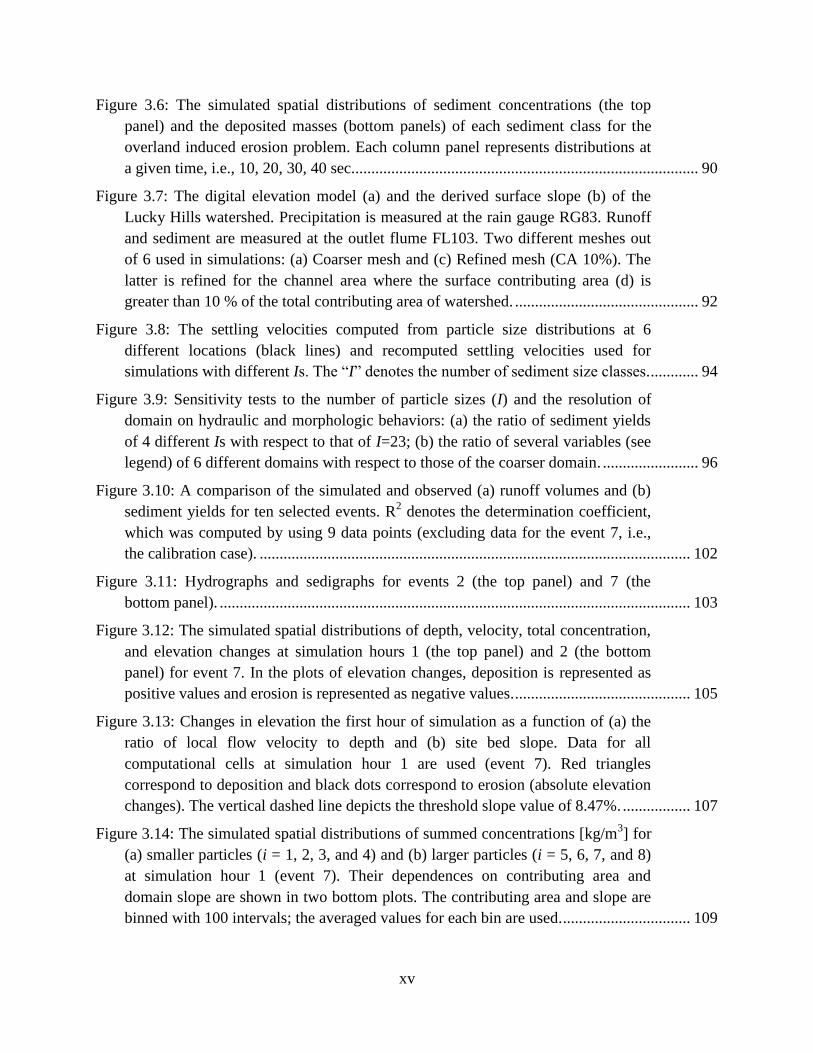
Figure 3.6: The simulated spatial distributions of sediment concentrations (the top

panel) and the deposited masses (bottom panels) of each sediment class for the

overland induced erosion problem. Each column panel represents distributions at

a given time, i.e., 10, 20, 30, 40 sec....................................................................................... 90

Figure 3.7: The digital elevation model (a) and the derived surface slope (b) of the

Lucky Hills watershed. Precipitation is measured at the rain gauge RG83. Runoff

and sediment are measured at the outlet flume FL103. Two different meshes out

of 6 used in simulations: (a) Coarser mesh and (c) Refined mesh (CA 10%). The

latter is refined for the channel area where the surface contributing area (d) is

greater than 10 % of the total contributing area of watershed. .............................................. 92

Figure 3.8: The settling velocities computed from particle size distributions at 6

different locations (black lines) and recomputed settling velocities used for

simulations with different Is. The “I” denotes the number of sediment size classes. ............ 94

Figure 3.9: Sensitivity tests to the number of particle sizes (I) and the resolution of

domain on hydraulic and morphologic behaviors: (a) the ratio of sediment yields

of 4 different Is with respect to that of I=23; (b) the ratio of several variables (see

legend) of 6 different domains with respect to those of the coarser domain. ........................ 96

Figure 3.10: A comparison of the simulated and observed (a) runoff volumes and (b)

sediment yields for ten selected events. R2 denotes the determination coefficient,

which was computed by using 9 data points (excluding data for the event 7, i.e.,

the calibration case). ............................................................................................................ 102

Figure 3.11: Hydrographs and sedigraphs for events 2 (the top panel) and 7 (the

bottom panel). ...................................................................................................................... 103

Figure 3.12: The simulated spatial distributions of depth, velocity, total concentration,

and elevation changes at simulation hours 1 (the top panel) and 2 (the bottom

panel) for event 7. In the plots of elevation changes, deposition is represented as

positive values and erosion is represented as negative values. ............................................ 105

Figure 3.13: Changes in elevation the first hour of simulation as a function of (a) the

ratio of local flow velocity to depth and (b) site bed slope. Data for all

computational cells at simulation hour 1 are used (event 7). Red triangles

correspond to deposition and black dots correspond to erosion (absolute elevation

changes). The vertical dashed line depicts the threshold slope value of 8.47%. ................. 107

Figure 3.14: The simulated spatial distributions of summed concentrations [kg/m3] for

(a) smaller particles (i = 1, 2, 3, and 4) and (b) larger particles (i = 5, 6, 7, and 8)

at simulation hour 1 (event 7). Their dependences on contributing area and

domain slope are shown in two bottom plots. The contributing area and slope are

binned with 100 intervals; the averaged values for each bin are used. ................................ 109

xvi

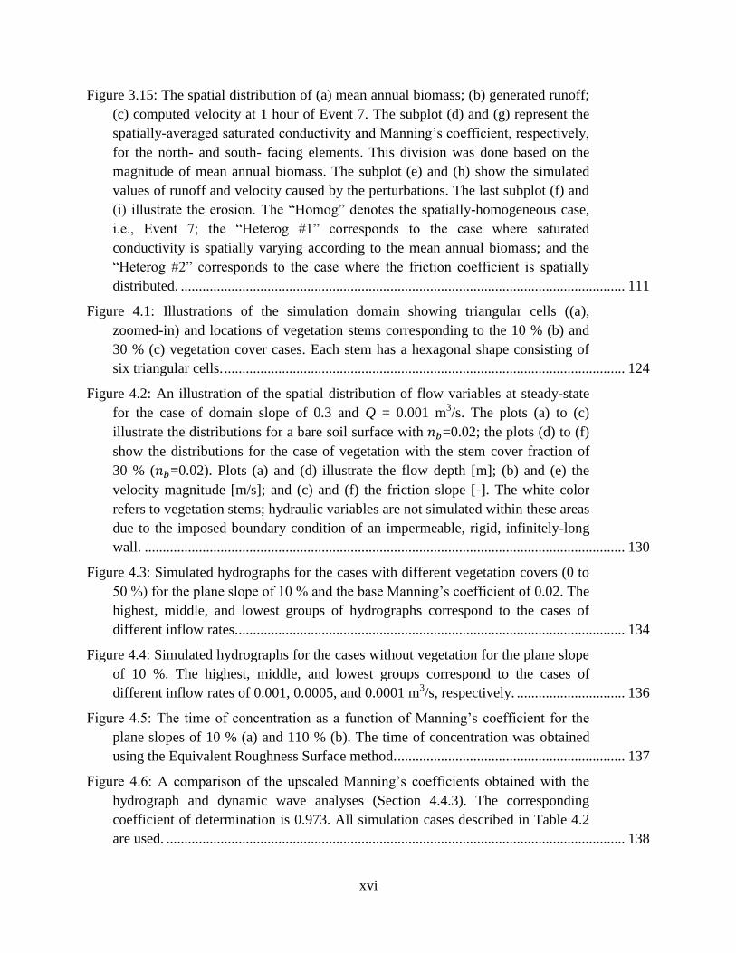
Figure 3.15: The spatial distribution of (a) mean annual biomass; (b) generated runoff;

(c) computed velocity at 1 hour of Event 7. The subplot (d) and (g) represent the

spatially-averaged saturated conductivity and Manning‟s coefficient, respectively,

for the north- and south- facing elements. This division was done based on the

magnitude of mean annual biomass. The subplot (e) and (h) show the simulated

values of runoff and velocity caused by the perturbations. The last subplot (f) and

(i) illustrate the erosion. The “Homog” denotes the spatially-homogeneous case,

i.e., Event 7; the “Heterog #1” corresponds to the case where saturated

conductivity is spatially varying according to the mean annual biomass; and the

“Heterog #2” corresponds to the case where the friction coefficient is spatially

distributed. ........................................................................................................................... 111

Figure 4.1: Illustrations of the simulation domain showing triangular cells ((a),

zoomed-in) and locations of vegetation stems corresponding to the 10 % (b) and

30 % (c) vegetation cover cases. Each stem has a hexagonal shape consisting of

six triangular cells. ............................................................................................................... 124

Figure 4.2: An illustration of the spatial distribution of flow variables at steady-state

for the case of domain slope of 0.3 and Q = 0.001 m3/s. The plots (a) to (c)

illustrate the distributions for a bare soil surface with =0.02; the plots (d) to (f)

show the distributions for the case of vegetation with the stem cover fraction of

30 % ( =0.02). Plots (a) and (d) illustrate the flow depth [m]; (b) and (e) the

velocity magnitude [m/s]; and (c) and (f) the friction slope [-]. The white color

refers to vegetation stems; hydraulic variables are not simulated within these areas

due to the imposed boundary condition of an impermeable, rigid, infinitely-long

wall. ..................................................................................................................................... 130

Figure 4.3: Simulated hydrographs for the cases with different vegetation covers (0 to

50 %) for the plane slope of 10 % and the base Manning‟s coefficient of 0.02. The

highest, middle, and lowest groups of hydrographs correspond to the cases of

different inflow rates. ........................................................................................................... 134

Figure 4.4: Simulated hydrographs for the cases without vegetation for the plane slope

of 10 %. The highest, middle, and lowest groups correspond to the cases of

different inflow rates of 0.001, 0.0005, and 0.0001 m3/s, respectively. .............................. 136

Figure 4.5: The time of concentration as a function of Manning‟s coefficient for the

plane slopes of 10 % (a) and 110 % (b). The time of concentration was obtained

using the Equivalent Roughness Surface method. ............................................................... 137

Figure 4.6: A comparison of the upscaled Manning‟s coefficients obtained with the

hydrograph and dynamic wave analyses (Section 4.4.3). The corresponding

coefficient of determination is 0.973. All simulation cases described in Table 4.2

are used. ............................................................................................................................... 138

xvii

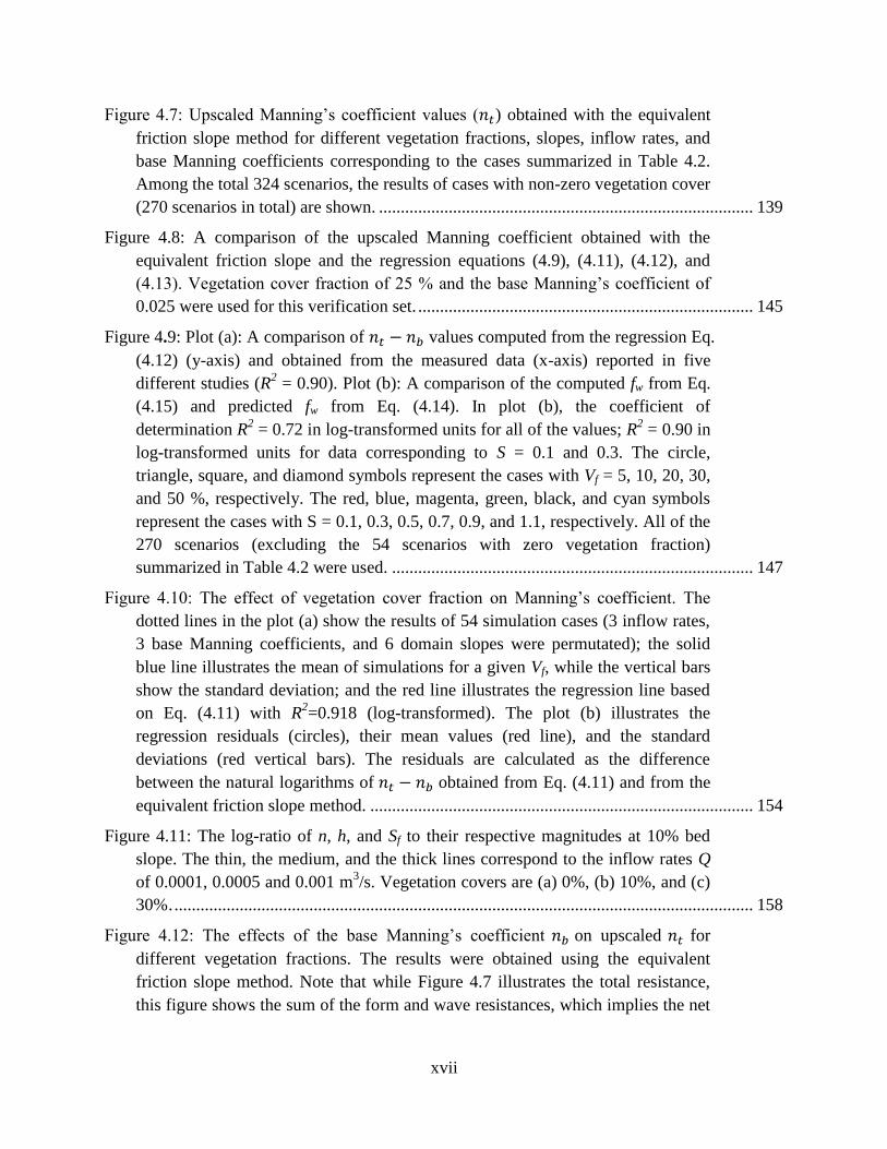
Figure 4.7: Upscaled Manning‟s coefficient values ( ) obtained with the equivalent

friction slope method for different vegetation fractions, slopes, inflow rates, and

base Manning coefficients corresponding to the cases summarized in Table 4.2.

Among the total 324 scenarios, the results of cases with non-zero vegetation cover

(270 scenarios in total) are shown. ...................................................................................... 139

Figure 4.8: A comparison of the upscaled Manning coefficient obtained with the

equivalent friction slope and the regression equations (4.9), (4.11), (4.12), and

(4.13). Vegetation cover fraction of 25 % and the base Manning‟s coefficient of

0.025 were used for this verification set. ............................................................................. 145

Figure 4.9: Plot (a): A comparison of values computed from the regression Eq.

(4.12) (y-axis) and obtained from the measured data (x-axis) reported in five

different studies (R2 = 0.90). Plot (b): A comparison of the computed fw from Eq.

(4.15) and predicted fw from Eq. (4.14). In plot (b), the coefficient of

determination R2 = 0.72 in log-transformed units for all of the values; R

2 = 0.90 in

log-transformed units for data corresponding to S = 0.1 and 0.3. The circle,

triangle, square, and diamond symbols represent the cases with Vf = 5, 10, 20, 30,

and 50 %, respectively. The red, blue, magenta, green, black, and cyan symbols

represent the cases with S = 0.1, 0.3, 0.5, 0.7, 0.9, and 1.1, respectively. All of the

270 scenarios (excluding the 54 scenarios with zero vegetation fraction)

summarized in Table 4.2 were used. ................................................................................... 147

Figure 4.10: The effect of vegetation cover fraction on Manning‟s coefficient. The

dotted lines in the plot (a) show the results of 54 simulation cases (3 inflow rates,

3 base Manning coefficients, and 6 domain slopes were permutated); the solid

blue line illustrates the mean of simulations for a given Vf, while the vertical bars

show the standard deviation; and the red line illustrates the regression line based

on Eq. (4.11) with R2=0.918 (log-transformed). The plot (b) illustrates the

regression residuals (circles), their mean values (red line), and the standard

deviations (red vertical bars). The residuals are calculated as the difference

between the natural logarithms of obtained from Eq. (4.11) and from the

equivalent friction slope method. ........................................................................................ 154

Figure 4.11: The log-ratio of n, h, and Sf to their respective magnitudes at 10% bed

slope. The thin, the medium, and the thick lines correspond to the inflow rates Q

of 0.0001, 0.0005 and 0.001 m3/s. Vegetation covers are (a) 0%, (b) 10%, and (c)

30% . ..................................................................................................................................... 158

Figure 4.12: The effects of the base Manning‟s coefficient on upscaled for

different vegetation fractions. The results were obtained using the equivalent

friction slope method. Note that while Figure 4.7 illustrates the total resistance,

this figure shows the sum of the form and wave resistances, which implies the net

xviii

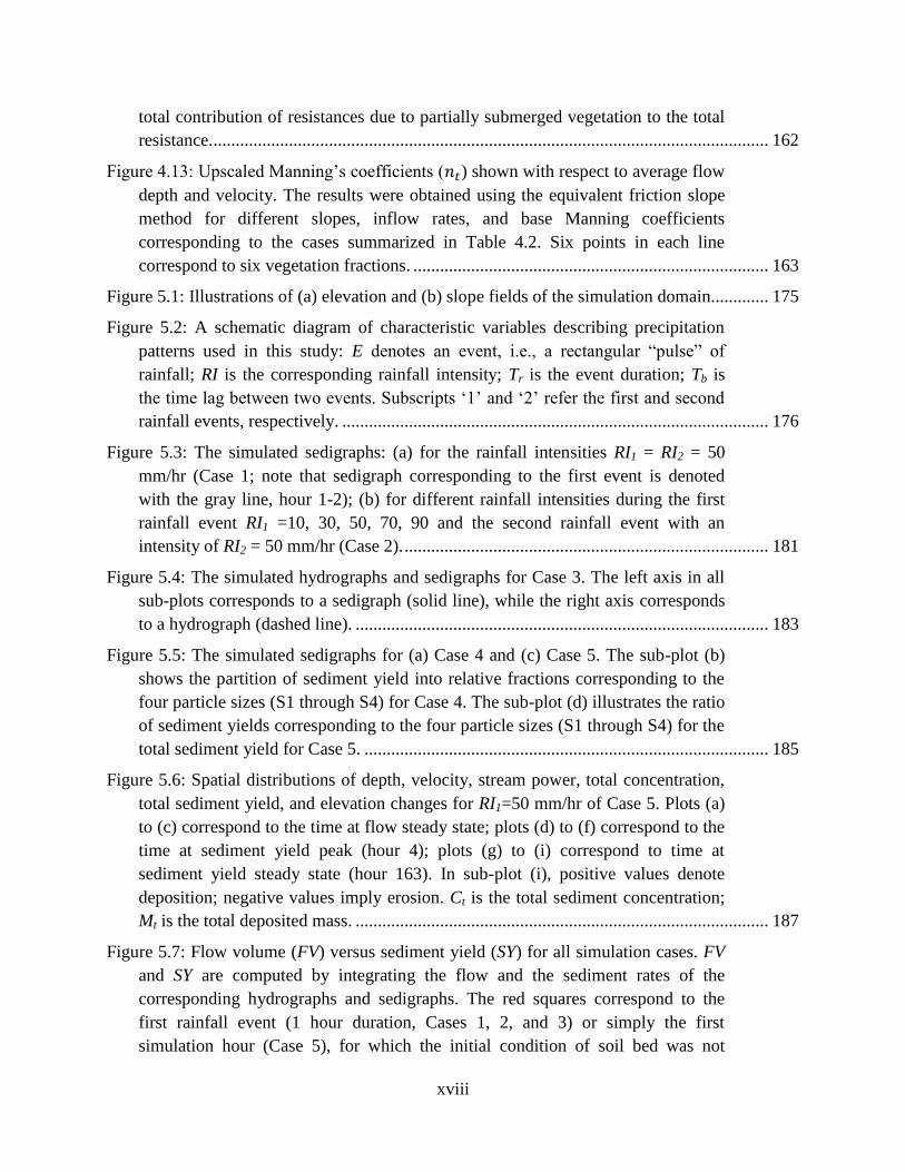
total contribution of resistances due to partially submerged vegetation to the total

resistance. ............................................................................................................................. 162

Figure 4.13: Upscaled Manning‟s coefficients ( ) shown with respect to average flow

depth and velocity. The results were obtained using the equivalent friction slope

method for different slopes, inflow rates, and base Manning coefficients

corresponding to the cases summarized in Table 4.2. Six points in each line

correspond to six vegetation fractions. ................................................................................ 163

Figure 5.1: Illustrations of (a) elevation and (b) slope fields of the simulation domain............. 175

Figure 5.2: A schematic diagram of characteristic variables describing precipitation

patterns used in this study: E denotes an event, i.e., a rectangular “pulse” of

rainfall; RI is the corresponding rainfall intensity; Tr is the event duration; Tb is

the time lag between two events. Subscripts „1‟ and „2‟ refer the first and second

rainfall events, respectively. ................................................................................................ 176

Figure 5.3: The simulated sedigraphs: (a) for the rainfall intensities RI1 = RI2 = 50

mm/hr (Case 1; note that sedigraph corresponding to the first event is denoted

with the gray line, hour 1-2); (b) for different rainfall intensities during the first

rainfall event RI1 =10, 30, 50, 70, 90 and the second rainfall event with an

intensity of RI2 = 50 mm/hr (Case 2). .................................................................................. 181

Figure 5.4: The simulated hydrographs and sedigraphs for Case 3. The left axis in all

sub-plots corresponds to a sedigraph (solid line), while the right axis corresponds

to a hydrograph (dashed line). ............................................................................................. 183

Figure 5.5: The simulated sedigraphs for (a) Case 4 and (c) Case 5. The sub-plot (b)

shows the partition of sediment yield into relative fractions corresponding to the

four particle sizes (S1 through S4) for Case 4. The sub-plot (d) illustrates the ratio

of sediment yields corresponding to the four particle sizes (S1 through S4) for the

total sediment yield for Case 5. ........................................................................................... 185

Figure 5.6: Spatial distributions of depth, velocity, stream power, total concentration,

total sediment yield, and elevation changes for RI1=50 mm/hr of Case 5. Plots (a)

to (c) correspond to the time at flow steady state; plots (d) to (f) correspond to the

time at sediment yield peak (hour 4); plots (g) to (i) correspond to time at

sediment yield steady state (hour 163). In sub-plot (i), positive values denote

deposition; negative values imply erosion. Ct is the total sediment concentration;

Mt is the total deposited mass. ............................................................................................. 187

Figure 5.7: Flow volume (FV) versus sediment yield (SY) for all simulation cases. FV

and SY are computed by integrating the flow and the sediment rates of the

corresponding hydrographs and sedigraphs. The red squares correspond to the

first rainfall event (1 hour duration, Cases 1, 2, and 3) or simply the first

simulation hour (Case 5), for which the initial condition of soil bed was not

xix

„disturbed‟ (i.e., intact soil bed condition). Black stars correspond to either the

second event (Cases 1, 2, and 3 in sub-plots (a)-(c)), the entire single event (Cases

3 and 4, sub-plots (d)-(e)), or hourly volumes (Case 5, sub-plot (f)). Specifically,

sub-plots (d) and (e) illustrate FVt and SYt that were computed for the entire

simulation period of Cases 3 and 4 to ensure the same runoff volume. Sub-plot (f)

illustrates a regression between hourly sediment yield (SYhr) and flow (FVhr) of

Case 5. .................................................................................................................................. 190

Figure 5.8: The partition into relative fractions corresponding to the four particle sizes

(S1 to S4) of sediment yield (SYi,2) generated by the second event for (a) Case 2

and (c) Case 3; and the partition of spatially-averaged deposited mass

immediately prior to the second event (Mi,2ini

) for (b) Case 2 and (d) Case 3. All

sub-plots correspond to the results of RI2=50 mm/hr. ......................................................... 196

Figure 5.9: An illustration of dynamic, unsteady evolution of erosion and sediment

transport response to a continuous rainfall of RI1 = 50 mm/hr simulated in Case 5.

The temporal evolution of (a) the hourly flow volume (FVhr) and (b) the hourly

instantaneous, spatially-averaged total concentrations (Ct,hrini

) and total deposited

mass (Mt,hrini

) as well as the total sediment yield (SYt,hr). The left axis is used for

Mt,hrini

and Ct,hrini

, while the right axis is used for SYt,hr. The two time scales, t1 and

t2, are identified with the two vertical dashed lines; the three corresponding phases

(I, II, and III) are also illustrated. The results obtained for the other rainfall

intensities and also specific for each particle size are provided in Figure 5.10. .................. 198

Figure 5.10: The time series of spatially-averaged concentration (Chrini

), deposited

mass (Mhrini

), and the outlet sediment yield (SYhr) as bulk characteristics (column

a) and specific for each particle size (columns b, c, d, and e). Simulation results

are for Case 5. The five sub-plots in the same row correspond to the same rainfall

intensity: from 10 mm/hr in the top row, to 90 mm/hr in the bottom row. In each

sub-plot, the left axis is used for Mhrini

and Chrini

, while the right axis is used for

SYhr. Two vertical dotted lines represent the time to peak (t1) and the time at

steady state (t2), respectively. .............................................................................................. 201

Figure 5.11: The Shields parameter related to the two time scales, the time to peak (t1)

and the time to steady state (t2): the green dashed lines correspond to t1, while the

red dashed lines correspond to t2. For S4 („+‟ symbol), t1 and t2 are overlapped

and for RI1=10 mm/hr, steady state is not reached. ............................................................. 202

Figure 5.12: An illustration of dynamic, unsteady evolution of erosion and sediment

transport response to a continuous rainfall of RI1 = 50 mm/hr simulated in Case 5.

The cumulative total sediment yield resolved at the hourly scale SYt,hrcum

plotted

against the spatially-averaged, species-specific (for the four particle sizes, S1 to

S4) (c) concentration Ci,hrini

and (d) deposited mass Mi,hrini

. The two time scales,

t1 and t2, are identified with the two horizontal dashed lines; the three

xx

corresponding phases (I, II, and III) are also illustrated. The results obtained for

the other rainfall intensities and also specific for each particle size are provided in

Figure 5.13. .......................................................................................................................... 205

Figure 5.13: The cumulative total sediment yield resolved at the hourly scale (SYt,hrcum

)

versus the hourly instantaneous, spatially-averaged (a) concentrations (Ci,hrini

) and

(b) deposited mass (Mi,hrini

) corresponding to four particle sizes (S1 to S4) and

five rainfall intensities (RI1,) of 10, 30, 50, 70, and 90 for Case 5. ..................................... 206

Figure 6.1: Parameters of the microcanonical disaggregation model for the location of

Watkinsville, GA. The rainfall data for a station at the Athens airport are used.

The left plot shows the probability that the cascade weight is 0 or 1 against the

time scale, while the right plot shows the parameter of Beta distribution for the

cascade weights. The dashed lines are a fitted logarithmic function (left plot) and

a fitted power law (right plot). The blue circles indicate the time scales over

which the models disaggregate rainfall.. ............................................................................. 226

Figure 6.2: An example of generated rainfall series. The top plot is first based on the

total amount and duration of storm and then aggregated into rainfall series with 5,

15, 30, and 60 minute intervals in order to verify that the disaggregated storm

characteristics satisfy the peak intensities over these intervals. .......................................... 227

Figure 6.3: A comparison of runoff and sediment yield obtained from observed date

and simulations. The five observed data values correspond to observations at 5

plots at the Watkinsville, GA, for a storm event starting on 19th

of October in

1950. The green circles indicate the simulation results for 15 different

disaggregation rainfall inputs. ............................................................................................. 230

xxi

LIST OF APPENDICES

A. Error Indices. .......................................................................................................................... 234

B. Eigenvalues and eigenvectors of Jacobian ............................................................................. 237

xxii

ABSTRACT

Watershed systems supply services and goods to human society. They should be

sustainable, maintain natural structure and function, and continue to meet societal needs in the

long-term. Numerous efforts investigated the effects of climate change on watershed components.

However, comprehensive studies of climate impacts relevant to the scale of human decisions

have been extremely limited. One of the goals of this dissertation is to develop a holistic, multi-

scale watershed model that describes essential physical processes. A coupling framework

between hydrologic processes, hydrodynamics, and soil erosion and sedimentation is developed

and presented. A previously existing model describing hydrological processes (tRIBS) has been

integrated with a solution of the Saint-Venant shallow water equations (OFM) and the Hairsine-

Rose formulation of erosion and deposition processes (HRM). The system of equations is

resolved using the finite volume method based on the Roe‟s approximate Riemann solver on an

unstructured grid. The resultant tRIBS-OFM-HRM model is one of the most comprehensive,

process-scale tools required for evaluations of climate signals that propagate through a non-linear

hydrological system.

The model has been used in several basic science applications. First, it has been applied

to address the problem of roughness upscaling for areas covered by partially submerged

obstacles, such as vegetated hillslopes. Two approaches, “Equivalent Roughness Surface” and

the “Equivalent Friction Slope”, for computing the upscaled Manning roughness coefficient are

xxiii

proposed. Predictive equations with several prognostic variables are developed to quantify the

additional resistance caused by partially submerged vegetation. The effects of all independent

variables are quantitatively investigated.

Second, the coupled model has been used to address a possible mechanism leading to the

non-uniqueness of soil erosion. It is attributed to two major conflicting effects: erosion

enhancement, due to supply of highly erodible sediment, and erosion impediment, due to

formation of a shielding layer that constrains the availability of lighter particles overlain by

heavier sediment. Two characteristic time scales, the time to peak and the time to steady-state,

are shown to separate three characteristic periods that correspond to flow-limited, source-limited,

and steady-state regimes. These time scales are demonstrated to be log-linearly and negatively

related to the spatially averaged Shields parameter.

1

CHAPTER I

Introduction

1.1 Motivation of a holistic, multi-scale, coupled approach

1.1.1 Climate change and human activity in watershed systems

Human societies require services and goods supplied by watershed systems, which should

be sustainable, maintain natural structure and function, and continue to meet societal needs in the

long-term [Meyer and Pulliam, 1992]. However, the world is undergoing a period of rapid

climate change, rarely experienced in the past [IPCC (Intergovernmental Panel on Climate

Change), 2001; 2007]. Its impacts, in concert with other human pressures, such as the

accelerated rates of water re-allocation and consumption, promise to alter the character and

services of watershed systems. Global-scale climate change and local-scale human impacts on

landuse inevitably affect the state of the atmosphere, surface and subsurface processes,

streamflow, erosion and sedimentation. They may lead to a variety of undesirable implications.

Figure 1.1 shows one striking example of such changes through aerial photographs of the

Muskegon River estuary [Baird, 2001]. This region has been highly affected by climate change

due to shorter and warmer winters, and warmer summer temperatures and extreme precipitation

2

events, resulting in a remarkable change of the estuary morphology over the period of the past

thirty years. Little information however exists to quantify the exact causes of this change, and

predicting how the current state will evolve further. Focused efforts are required to address the

short- and long-term effects of climate change on erosion, sediment transport and morphology in

earth-science disciplines.

Figure 1.1: Aerial photographs of the Muskegon River estuary (after Baird, 2001)

1.1.2 Significance and challenges of a multi-scale coupled approach

The processes of erosion and sedimentation originate at the watershed level: the

watershed-scale, hydrologic disturbances propagate into streamflow and alter the flow regime;

the flow process leads to erosion processes that modify landscape morphology. When considered

3

in the context of long-term effects of climate change on such important drivers as precipitation

and temperature, perturbations at larger scale impact local-scale hydrological signals, especially

evaporation and runoff, which subsequently affect streamflow variations. The flow motion

ultimately leads to an effect on sediment transport and erosion rates, and modifies the

morphology of the surface; the resultant morphologic change in turn affects the flow dynamics.

Therefore, modeling the impacts of climate change on landscape evolution, catchment

morphology and sediment yields requires a holistic approach, involving many significant

components such as hydrology, hydraulics, vegetation dynamics, erosion and sedimentation.

Any assessment of potential impact of climate change should consider all related

processes that occur different spatial and temporal scales, and employ an integrated approach

capable of simulating all involved process components simultaneously. Models including

individual components or a subset of coupled processes (e.g., hydrology-erosion or hydraulics-

erosion) have been previously developed with moderate-to-satisfactory success. However,

models including all critical process components have not yet been proposed. The likely reason

is the complexity of coupling, in which related processes operate at a range of temporal and

spatial scale. For example, climate change and morphologic variations are characteristic of

global spatial and long-term temporal scales; hydrologic processes are conveyed at the watershed

scale, over relatively short-term temporal scales; hydraulic and erosion processes are concerned

with a river-reach or a hillslope spatial, and short-term temporal scales (see Figure 1.2). Another

reason why fully coupled models have not been developed is because relevant processes extend

across several disciplines. The connection between hydrology and hydraulics in overland flow

modeling, and the effects of channel and hillslope erosion processes on the total sediment budget

in watershed erosion modeling have not been fully considered at the relevant level of detail.

4

Figure 1.2: A space-time diagram showing characteristic ranges of modeling approaches.

1.1.3 Characteristics of watershed systems: connectivity and non-linearity

A critical feature of watershed systems is their connectivity [Michaelides and Chappell,

2009], i.e., hydrologically mediated transfer of mass, momentum, energy, or organisms within or

between basin compartments. Disturbances arising at any scale will necessarily propagate

downstream, e.g., large-scale climate perturbations will affect local-scale hydrologic processes,

flow regime, erosion, and stream sedimentation. The local-scale effects can be responsible for

damages to aquatic habitats and disruption of ecological services [Mooney et al., 2009]. Due to

the tremendous disparity of involved spatiotemporal scales, we currently lack assessment tools

that explicitly consider connectivity of watershed processes (and are also relevant to the “scales

5

of human decisions” and ecosystem services). Further, watersheds are non-linear systems; their

dynamics depend on „convective‟ and „dissipative‟ characteristics of involved processes. The

latter are inevitably time- and space- varying and depend on forcings, and initial and boundary

conditions. Physically-based, “process-scale” approaches considering both connectivity and non-

linearity of watershed systems are required for robust assessments of non-linear effects.

Compensation and mitigation of climate impacts are also limited due to the difficulty of

evaluation of climate signals that propagate through a non-linear hydrological system.

1.1.4 The need for a holistic, multi-scale, coupled model

Comprehensive studies of climate impacts relevant to the scale of human decisions, such

as an agricultural field, a stream reach, or a flood-control structure, have been extremely limited.

For example, global and regional scale studies have examined the impact of projected climate

change on a number of large-scale hydrologic variables [Barnett et al., 2005; Milly et al., 2005].

They however lacked the propagation of this information through watershed systems to seek a

more detailed level of flow characteristics (i.e., those that extend beyond the traditional metrics

of bulk, area-integrated runoff) that can be directly responsible for major impacts on water

quality and aquatic habitat characteristics. At the other end of research spectrum, hydraulic

engineers carried out stream-reach scale studies addressing flow regimes and details of flow

dynamics. However, by assuming artificial boundary conditions these studies have failed to

connect to catchment- and larger-scale (e.g., climate) information. This has essentially

“disengaged” channel flow from watershed processes [Milly et al., 2002; Arnell, 2003;

Cherkauer and Sinha, 2010]. As a result, at present we entirely lack assessments of climate

impacts on spatially-distributed flow characteristics, water quality, and aquatic systems through a

6

holistic, multi-scale approach. Understanding and predicting the corresponding shifts across a

range of space-time scales is one of the most fundamental, yet poorly quantified challenges

facing society today.

1.2 Research scope

A new holistic, coupled model that considers hydrological processes, flow dynamics, and

erosion and sediment transport is developed and presented in detail in the following chapters.

Chapter II of this dissertation addresses a coupling framework between a hydrologic

model and a hydrodynamic model. The resultant coupled model, tRIBS-OFM, considers

spatially-distributed, physically-based hydrologic processes over the land-surface and subsurface

by using tRIBS (Triangulated irregular network – based, Real time Integrated Basin Simulator);

the hydrodynamic component is the Overland Flow Model (OFM), which solves the two-

dimensional Saint-Venant (shallow-water) equations using Roe‟s approximate Riemann solver

on an unstructured grid. The original OFM formulation targeted hydraulic applications and did

not provide an accurate solution for partially-submerged mesh cells. Modifications of the

hydrodynamic model are proposed in this chapter by applying a new method of reconstruction of

variables. Several comparisons with analytical solutions, observed data, and other numerical

models, and two applications to a synthetic domain and a real-world basin, the Peacheater Creek

watershed located near Christie, OK, U.S.A., are also presented.

Chapter III outlines a novel, two-dimensional, physically-based model of soil erosion and

sediment transport. The Hairsine-Rose formulation of erosion and deposition processes is used to

account for size-selective sediment transport and differentiate bed material into original and

7

deposited soil layers. The formulation has been integrated within the framework of the

hydrologic and hydrodynamic model tRIBS-OFM. The resultant model explicitly couples the

hydrodynamic formulation with the advection-dominated transport equations for sediment of

multiple particle sizes. The finite volume method based on Roe‟s approximate Riemann solver

on an unstructured grid is described with the system of equations including both the Saint-

Venant and the Hairsine-Rose equations. The chapter also provides verifications with analytical

solutions and empirical data for two benchmark cases; two sensitivity tests to grid resolution and

the number of particle sizes; and an application at the catchment scale for the Lucky Hills

watershed located in southeastern Arizona, U.S.A. Additionally, spatial output has been analyzed

and the driving role of topography in erosion processes is discussed.

The developed coupled model has been used in several basic science applications. In

Chapter IV the developed model is used to numerically investigate the characteristics of

upscaling the Manning resistance coefficient for areas covered by partially submerged vegetation

elements, such as shrub or tree stems. A number of high-resolution hydrodynamic simulations

corresponding to scenarios with different domain slopes, inflow rates, bed roughness, and

vegetation cover fractions are carried out. Using simulations performed at fine space-time scales,

two methods are developed for computing the upscaled Manning coefficient, called “Equivalent

Roughness Surface (ERS)” and “Equivalent Friction Slope (EFS)”. Further, the effects of four

independent variables on the total Manning coefficient are discussed. A regression relation that

includes all four variables and the additional resistance due to partially submerged vegetation

representing the sum of the form and wave resistances is presented. The upscaled values

computed from the developed regression relation are validated through a comparison with

8

estimates reported in five different empirical studies. The simulated wave resistance coefficients

are also compared with those predicted from an equation proposed in a previous study.

Chapter V addresses possible reasons leading to non-uniqueness of soil erosion

susceptibility; specifically, the role of shielding layer in multi-size particle dynamics are

discussed. To obtain relevant insights, 95 numerical simulations using synthetic storms of

varying intensity, duration, and lag time between successive events (to obtain different runoff

conditions in a zero-order catchment) are presented. The design targets to generate flow and

„perturb‟ soil substrate by a first rainfall event, creating the initial conditions of flow and

sediment prior to the onset of a subsequent rainfall event. Due to the affected particle size

distribution, a shielding layer composed of larger particles is formed in some cases. The results

indicate that unless the initial condition of flow and sediment spatial distribution is identical, the

same volume of runoff can generate different total sediment yields even in conditions of identical

rainfall forcing. The reasons for non-uniqueness are attributed to two major conflicting effects

occurring during the erosion process: erosion enhancement, because of supply of highly erodible

sediment from upstream areas, and erosion impediment, because of formation of a shielding

layer that constrains the availability of lighter particles due to heavier sediment. Long-term

simulations with continuous rainfall also show that a peculiar feature of sediment yield series is

the existence of maximum before the steady-state is reached. Two characteristic time scales, the

time to peak and the time to steady-state, are eventually presented to separate three characteristic

periods that correspond to flow-limited, source-limited, and steady-state regimes

Chapter VI summarizes this dissertation and addresses perspectives for ongoing and

future studies. Major conclusions and critical assumptions of conducted research, and a

feasibility study for national assessment of soil loss are presented. The latter objective focuses on

9

investigating interactions among the components of agricultural farming such as tillage,

conservative practices, and landuse management. It is conjectured that through extensive

observations of USLE (Universal Soil Loss Equation) database, the developed model can be

further verified, and representative parameter sets for complex conditions can be obtained to

carry out relevant assessments. Lastly, the uncertainty and non-linearity of processes of erosion

and sedimentation related to climate projections and hydrological conditions such as extreme

precipitation and dynamically varying vegetation state during growing and dormant seasons is

argued to be a fruitful research agenda that will be addressed in future.

10

CHAPTER II

Coupled modeling of hydrologic and hydrodynamic processes including

overland and channel flow: “tRIBS-OFM”

2.1 Introduction

A description of overland and channel flow processes plays a crucial role in a variety of

hydrologic, hydraulic, agricultural, and ecological problems, such as rainfall-runoff modeling,

flood routing, sedimentation and erosion, irrigation and drainage, and environmental change of

aquatic habitats. In particular, the consequences of flow-related events were recently addressed

in the light of abnormal meteorological phenomena occurring possibly due to climate change

[Chen et al., 2008; Makkeasorn et al., 2008; L H Li et al., 2010], i.e., more violent storms with

higher precipitation intensities, leading to extreme flooding events [Dankers and Feyen, 2008;

Kay et al., 2009; Mantua et al., 2010]. Such abnormal events may have numerous undesirable

implications for human life and damage of property, as well as ecological consequences.

Therefore, a number of studies have investigated the rainfall-runoff mechanism and ways to

diminish human and property damages from floods by using physically-based hydrologic and

hydraulic models for predictions [Hunter et al., 2007].

11

Overland flow can be regarded as the propagation of shallow water waves, which can be

mathematically represented by the Saint-Venant equations, the so called “dynamic wave”

formulation, or by their simplified versions, e.g., the inertia-free and kinematic approximations

[Katopodes, 1982]. In the dynamic wave model, the momentum equation is balanced among

inertial, pressure, gravitational, frictional, and momentum source terms, while in the inertia-free

model, the local and convective acceleration terms are neglected; in the kinematic wave model,

not only these but the pressure term is also neglected. Researchers and engineers have

historically developed hydrologic models based on simplified approximations that can be

applicable for problems of flood wave propagation in steep terrain because of their

computational efficiency or simplicity [Parlange et al., 1981; Hromadka et al., 1985; Hromadka

and Nestlinger, 1985; Govindaraju et al., 1990; Keskin and Agiralioglu, 1997; Odai, 1999;

Moramarco and Singh, 2000; Wang et al., 2002; Downer and Ogden, 2004; Panday and

Huyakorn, 2004; Tsai and Yang, 2005; Howes et al., 2006; Kollet and Maxwell, 2006a; Du et al.,

2007; Alonso et al., 2008; Prestininzi, 2008; Goderniaux et al., 2009; J K Huang and Lee, 2009].

However, simplified models have several limitations for applications in cases of flow over flat

slopes, flow into large reservoirs, flow reversals, and strong backwater conditions. These

limitations may seriously constrain the applicability of simplified models to a range of practical

problems as well as conditions of the changing world.

In order to enhance the applicability and accuracy of simplified models, several dynamic

wave models have been previously developed for simulating overland flow by calculating the

full version of the momentum equations in the Saint-Venant equations [Akanbi and Katopodes,

1988; DiGiammarco et al., 1996; Katopodes and Bradford, 1999; Horritt, 2002; Begnudelli and

Sanders, 2006; Gottardi and Venutelli, 2008]. However, the dynamic wave model formulation

12

requires detailed watershed topographic and channel cross sectional data and poses serious

challenges for the numerical solution when applied continuously over storm-interstorm periods.

Additionally, such models neglect a detailed description of crucial components of the hydrologic

processes, such as evapotranspiration, interception, infiltration, and groundwater dynamics.

These models treat these processes implicitly through “well-defined” inputs or assumptions to

compute the components of flow regime in terms of the maximum water depth, discharge and

velocities of flow as well as the maximum inundation area.

Runoff generation, the crucial process for simulating overland and channel flow, is highly

affected by the spatial variability of antecedent moisture and hydrologic processes of infiltration

and percolation, groundwater recharge/discharge, and evapotranspiration, as determined by the

spatial distribution of meteorological forcing. Because of the strong interdependence between

surface hydraulics and the subsurface hydrology, there has been an increased interest in recent

years in the development of coupled surface and subsurface models [Bixio et al., 2000;

VanderKwaak and Loague, 2001; Morita and Yen, 2002; Panday and Huyakorn, 2004; Kollet

and Maxwell, 2006a; Goderniaux et al., 2009; Camporese et al., 2010; Rihani et al., 2010; Shen

and Phanikumar, 2010]. All of these studies represent the flow processes in the variably

saturated zone by solving the Richards equation. The surface flow phenomenon is also

considered by solving different approximations of the Saint-Venant equations: the inertia-free

formulation is used most often, while the kinematic [Kollet and Maxwell, 2006b; Rihani et al.,

2010] and dynamic [Morita and Yen, 2002] forms were also proposed. The numerical simulation

of the coupled surface and subsurface equations is carried out using either an unstructured

triangular mesh [VanderKwaak and Loague, 2001; Goderniaux et al., 2009] or a rectangular grid

(the rest of the studies cited above). With the exception of the studies by Rihani et al. [2010] and

13

Shen and Phanikumar [2010], most of the above cited model developments focus on the

subsurface phenomena, simplistically describing above-surface processes (e.g.,

evapotranspiration). Energy exchanges between the subsurface and the atmosphere are neglected.

However, if one intends to take into account the spatiotemporal structure of runoff production

and the related effect on the flow regime, both a spatially-distributed, comprehensive hydrologic

model that considers all relevant processes, and a hydrodynamic model solving the full dynamic

equations have to be considered to accurately predict flow characteristics (e.g., depth, velocity

vectors, vorticities, shear stress, etc.).

A coupled model, tRIBS-OFM is introduced in this Chapter. The key features of the

tRIBS-OFM include 1) the generality of the dynamic wave formulation that can deal with

various boundary conditions and its numerical implementation based on an unstructured

triangular mesh; 2) the capability of applying the model for challenging hydrological situations,

such as a partially wetted domain and low-flow conditions; and 3) coupling of the hydrodynamic

component with a hydrological model, which provides a seamless transition from the

hydrometeorologic boundary conditions to those that are required by the hydrodynamic

simulation at the catchment scale.

The overarching objective of the coupled framework is to quantitatively predict the

spatial and temporal hydrologic response to imposed scenarios of climate change, land-use

variations, soil, and vegetation types in small- to large-scale basins. First, model backgrounds are

provided and modifications necessary for the coupled model are described. These modifications

are stressed because in large domains with both steep and flat slopes, the typical shallow water

solver developed for hydraulic applications does not accurately capture the flow regime in a

large number of partially-submerged cells of an unstructured grid. Next, model verifications are

14

carried out in which the simulation results are compared with analytical solutions, observed data,

and other numerical models; a one-dimensional plane and a V-shaped domain are used. The

effects of inertia and pressure terms in the momentum equation are investigated for the V-shaped

catchment. The results of using both the kinematic and dynamic formulations are also presented.

Lastly, applications to both a synthetic domain and the Peacheater Creek watershed (64 km2)

located near Christie, OK, are performed to illustrate the model multi-scale capabilities and the

feasibility of various aspects of watershed streamflow simulation: runoff production occurrences

and rates, streamflow, flow depth, velocities, and a reservoir problem.

2.2 Description of the coupled model

2.2.1 Model heritage: tRIBS

The coupled model presented in this study consists of a hydrologic model and a

hydrodynamic model. The hydrologic model, the TIN (Triangulated Irregular Network) - Based

Real Time Integrated Basin Simulator (tRIBS), has the capability to explicitly utilize a variety of

data, such as topography, soil type, land use, and vegetation. The tRIBS model is forced with

meteorological series that consist of precipitation, radiation, metrics of atmospheric turbulence,

temperature and humidity. The model simulates in a spatially-explicit manner a number of

hydrologic processes such as rainfall interception, evapotranspiration, infiltration with

continuous soil moisture accounting, lateral moisture transfer in the unsaturated and saturated

zones, and one-dimensional channel runoff routing. In particular, the model stresses the role of

topography in lateral soil moisture redistribution, accounting for the effects of spatially

heterogeneous and anisotropic soil in a simplified manner. The model computational basis,

structure, and the description of process parameterizations are detailed by Ivanov et al. [2004a].

15

A brief outline of the implemented process parameterizations is provided in the following and

summarized in Table 2.1.

For simulating precipitation interception, the Rutter canopy water balance model [Rutter

et al., 1971; Rutter et al., 1975] is used. Canopy water dynamics is species dependent

such that the parameters can vary for different vegetation types.

For estimating surface energy budget, shortwave and longwave radiation components are

simulated, accounting for geographic location, time of year, aspect and slope of the

element surface [Bras, 1990]. The combination equation [Penman, 1948; Monteith, 1965],

gradient [Entekhabi, 2000], and force-restore [Lin, 1980; Z Hu and Islam, 1995] methods

are used to estimate the latent, sensible, and ground heat fluxes at the land surface. An

optimum is sought in terms of the surface temperature that leads to the energy balance.

Soil water content in the root zone and top soil layer constrains evapotranspiration from

vegetated surfaces and bare soil. A species-dependent parameterization of stomatal

conductance allows for the diurnal variation of transpiration flux.

Latent heat energy is partitioned into evaporation from wet canopy, vegetation

transpiration, and bare soil evaporation; the latter two are limited by available moisture in

the soil zone, depending on vegetation fractional coverage of an element and canopy state.

For simulating the process of infiltration, an assumption of gravity-dominated flow in a

sloped column of heterogeneous, anisotropic soil is used, so that the effect of capillary

forces is approximated [Cabral et al., 1992; Ivanov et al., 2004a]. All soil parameters

described in Table 2.2 are allowed to vary in space over a heterogeneous basin area; there

are specific assumptions about changes in the soil saturated hydraulic conductivity that

are detailed in Ivanov et al. [2004a]. By considering the evolution of the wetting and top

16

fronts and the fluctuation of the water table in any given element, the vadose zone is

conceptualized with five states: initial, unsaturated, perched, surface saturated, and

completely saturated [Ivanov et al., 2004a]. The first three states are defined for cases

where the soil infiltration capacity is not constrained by the conductivity at the surface,

while the surface saturated state is generated when the soil‟s infiltration capacity is

constrained by the entire saturated profile that exhibits a decay of conductivity with depth.

In the unsaturated state, only the wetting front is present, while in the perched (surface

saturated) state, the top front is shallower than the wetting front (located at the soil

surface). For the fully saturated state, the soil infiltration capacity is zero. The unsaturated

and saturated zones are coupled, accounting for the interaction of the moving infiltration

front with a time-varying water table. Topography and soil control the magnitude of

lateral moisture transfer in the unsaturated zone. Continuous soil moisture accounting

allows the representations of both storm and interstorm conditions, thus permitting long-

term simulation over a range of hydrometeorological forcings.

For simulating the groundwater dynamics, a model based on the Boussinesq‟s equation

under the Dupuit-Forchheimer assumptions is used, allowing for a lateral water

redistribution in the saturated zone and its dynamic interactions with the unsaturated zone.

The lateral exchanges between contiguous elements are calculated by using the depth-

averaged aquifer transmissivity, and the local slope of water table.

Runoff generation is made possible via four mechanisms: saturation excess [Dunne and

Black, 1970], infiltration excess [Horton, 1933; Loague et al., 2010], perched subsurface

stormflow [Weyman, 1970], and groundwater exfiltration [Hursh and Brater, 1941].

Runoff is generated by representing the movement of infiltration fronts, water table

17

fluctuations, and lateral moisture fluxes in the unsaturated and saturated zones. The

runoff computed in this hydrologic module is used as input to the hydrodynamic overland

flow model.

A snowpack dynamic model has been recently added [Rinehart et al., 2008] that permits

the simulation of energy and mass budgets of snow-covered areas.

Table 2.1: A summary of processes considered in the hydrologic model tRIBS.

Processes Governing equations and methods

Rainfall interception Rutter canopy water balance model [Rutter et al., 1971; Rutter et al.,

1975]

Surface energy

balance

The combination equation method for latent heat flux [Penman, 1948;

Monteith, 1965], gradient method for sensible heat flux [Entekhabi,

2000], and force-restore method for ground water flux [Lin, 1980; Z Hu

and Islam, 1995]

Evapotranspiration The bare soil evaporation [Deardorff, 1978], canopy evaporation, and

transpiration [Eltahir and Bras, 1993]

Infiltration Gravity-dominated unsaturated flow [Cabral et al., 1992; Ivanov et al.,

2004a]

Groundwater

dynamics

Quasi-3D Boussinesq‟s equation under the Dupuit-Forchheimer

assumptions [Ivanov et al., 2004a]

Runoff generation Saturation excess [Dunne and Black, 1970], infiltration excess [Horton,

1933], perched stormflow [Weyman, 1970], and groundwater exfiltration

[Hursh and Brater, 1941]

Snowpack dynamics Snowpack dynamic model [Rinehart et al., 2008]

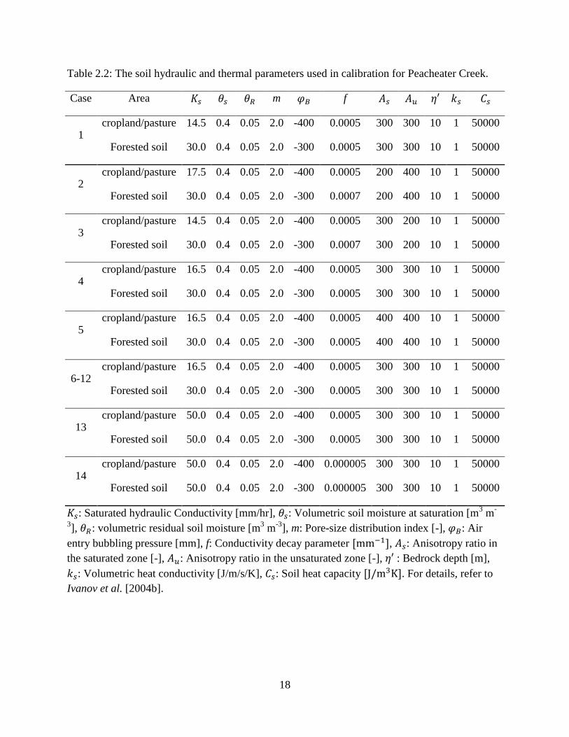
18

Table 2.2: The soil hydraulic and thermal parameters used in calibration for Peacheater Creek.

Case Area m f

1 cropland/pasture 14.5 0.4 0.05 2.0 -400 0.0005 300 300 10 1 50000

Forested soil 30.0 0.4 0.05 2.0 -300 0.0005 300 300 10 1 50000

2 cropland/pasture 17.5 0.4 0.05 2.0 -400 0.0005 200 400 10 1 50000

Forested soil 30.0 0.4 0.05 2.0 -300 0.0007 200 400 10 1 50000

3 cropland/pasture 14.5 0.4 0.05 2.0 -400 0.0005 300 200 10 1 50000

Forested soil 30.0 0.4 0.05 2.0 -300 0.0007 300 200 10 1 50000

4 cropland/pasture 16.5 0.4 0.05 2.0 -400 0.0005 300 300 10 1 50000

Forested soil 30.0 0.4 0.05 2.0 -300 0.0005 300 300 10 1 50000

5 cropland/pasture 16.5 0.4 0.05 2.0 -400 0.0005 400 400 10 1 50000

Forested soil 30.0 0.4 0.05 2.0 -300 0.0005 400 400 10 1 50000

6-12 cropland/pasture 16.5 0.4 0.05 2.0 -400 0.0005 300 300 10 1 50000

Forested soil 30.0 0.4 0.05 2.0 -300 0.0005 300 300 10 1 50000

13 cropland/pasture 50.0 0.4 0.05 2.0 -400 0.0005 300 300 10 1 50000

Forested soil 50.0 0.4 0.05 2.0 -300 0.0005 300 300 10 1 50000

14 cropland/pasture 50.0 0.4 0.05 2.0 -400 0.000005 300 300 10 1 50000

Forested soil 50.0 0.4 0.05 2.0 -300 0.000005 300 300 10 1 50000

: Saturated hydraulic Conductivity [mm/hr], : Volumetric soil moisture at saturation [m3 m

-

3], : volumetric residual soil moisture [m

3 m

-3], m: Pore-size distribution index [-], : Air

entry bubbling pressure [mm], f: Conductivity decay parameter , : Anisotropy ratio in

the saturated zone [-], : Anisotropy ratio in the unsaturated zone [-], : Bedrock depth [m],

: Volumetric heat conductivity [J/m/s/K], : Soil heat capacity . For details, refer to

Ivanov et al. [2004b].

19

2.2.2 Model heritage: OFM

The hydrodynamic Overland Flow Model (OFM) is a high resolution, depth-averaged,

two-dimensional finite volume model that solves the Saint-Venant equations on the basis of an

unstructured triangular grid. Early contributions to the numerical solution of the Saint-Venant

equations were made by Leendertse [1967], Liggett [1968], and Abbott [1974]. In this study,

Roe‟s approximate Riemann solver [Roe, 1981] is used to compute fluxes. The hydrodynamic

model was originally developed by Bradford and Katopodes [1999] to simulate turbidity currents

and was later used to model surface irrigation [Bradford and Katopodes, 2001]. It has been

previously successfully applied to a wide range of hydrodynamic scenarios [Bradford and

Sanders, 2002] and extended to an unstructured triangular mesh [Begnudelli and Sanders, 2006].

In order to enhance the run-time efficiency, a Local Time Stepping (LTS) scheme was developed

that showed an increased performance by 50 to 70 %, without a loss of accuracy or mass

conservation [Sanders, 2008]. The OFM is able to compute the depth of flow, the velocity field,

and the location and elevation of the free surface. A detailed outline of the governing equations,

Roe‟s approximate Riemann solver implemented in the model, boundary conditions, etc. are

provided in the Chapter III.

2.2.3 OFM modification

The original OFM was designed for hydraulic applications such as flooding and dam

break problems. In order to adapt the design to hydrologic applications, several modifications

have been made for calculating the flux, bottom slope, and friction slope terms by applying a

different reconstruction method of variables. Before describing these changes in the tRIBS-OFM

20

framework, the method for identifying partially-submerged cells, a situation frequently occurring

in hydrologic applications, is explained in the following.

The standard OFM design classifies the computational cells (i.e., triangles of unstructured

triangular mesh) into three different groups corresponding to fully-submerged (wet), partially-

submerged, and non-submerged (dry) conditions. The model first checks conditions at all cell

vertices. Similar to the published studies by Jones et al. [2008] and Camporese et al. [2010], the

model identifies “wet nodes” by comparing the depth at each vertex with a very small, pre-

defined tolerance value (e.g., ). The model then labels cells as “wet”, only if all vertices

have depths larger than the tolerance value. Cells under any other conditions are defined as “dry

cells”. Once a cell is identified as a “wet” cell, the model solves both the continuity and

momentum equations for this cell, yielding the x- and y- components of velocity of the flow.

However, if a cell has been identified as “dry”, the model sets the flow velocity to zero, and

therefore does not compute the momentum equations. This procedure prevents the numerical

instability that would be otherwise generated because of unrealistically high velocities that would

result from dividing the volume fluxes by very small depths. The condition of numerical

instability is the “classical” but critical problem of applying a fully dynamic model to a

hydrologic simulation with small runoff production.

The first difference in dealing with partially-submerged cells in hydrologic vs. hydraulic

applications concerns the existence of dry or “partially wet” cells. Hydraulic applications such as

flood propagation and wave runup involve a large number of initially wet cells (river or ocean)

and a distinct wet and dry boundary (floodplain or coastline). Several approaches have been

developed to track wet and dry fronts and handle the phenomenon by using information of

neighboring wet cells [Titov and Synolakis, 1995; Bradford and Sanders, 2002; Xia et al., 2010]

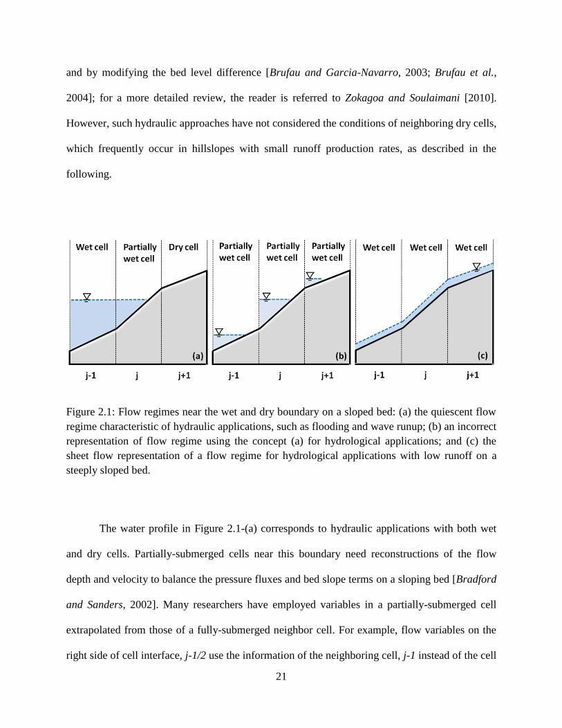
21

and by modifying the bed level difference [Brufau and Garcia-Navarro, 2003; Brufau et al.,

2004]; for a more detailed review, the reader is referred to Zokagoa and Soulaimani [2010].

However, such hydraulic approaches have not considered the conditions of neighboring dry cells,

which frequently occur in hillslopes with small runoff production rates, as described in the

following.

Figure 2.1: Flow regimes near the wet and dry boundary on a sloped bed: (a) the quiescent flow

regime characteristic of hydraulic applications, such as flooding and wave runup; (b) an incorrect

representation of flow regime using the concept (a) for hydrological applications; and (c) the

sheet flow representation of a flow regime for hydrological applications with low runoff on a

steeply sloped bed.

The water profile in Figure 2.1-(a) corresponds to hydraulic applications with both wet

and dry cells. Partially-submerged cells near this boundary need reconstructions of the flow

depth and velocity to balance the pressure fluxes and bed slope terms on a sloping bed [Bradford

and Sanders, 2002]. Many researchers have employed variables in a partially-submerged cell

extrapolated from those of a fully-submerged neighbor cell. For example, flow variables on the

right side of cell interface, j-1/2 use the information of the neighboring cell, j-1 instead of the cell

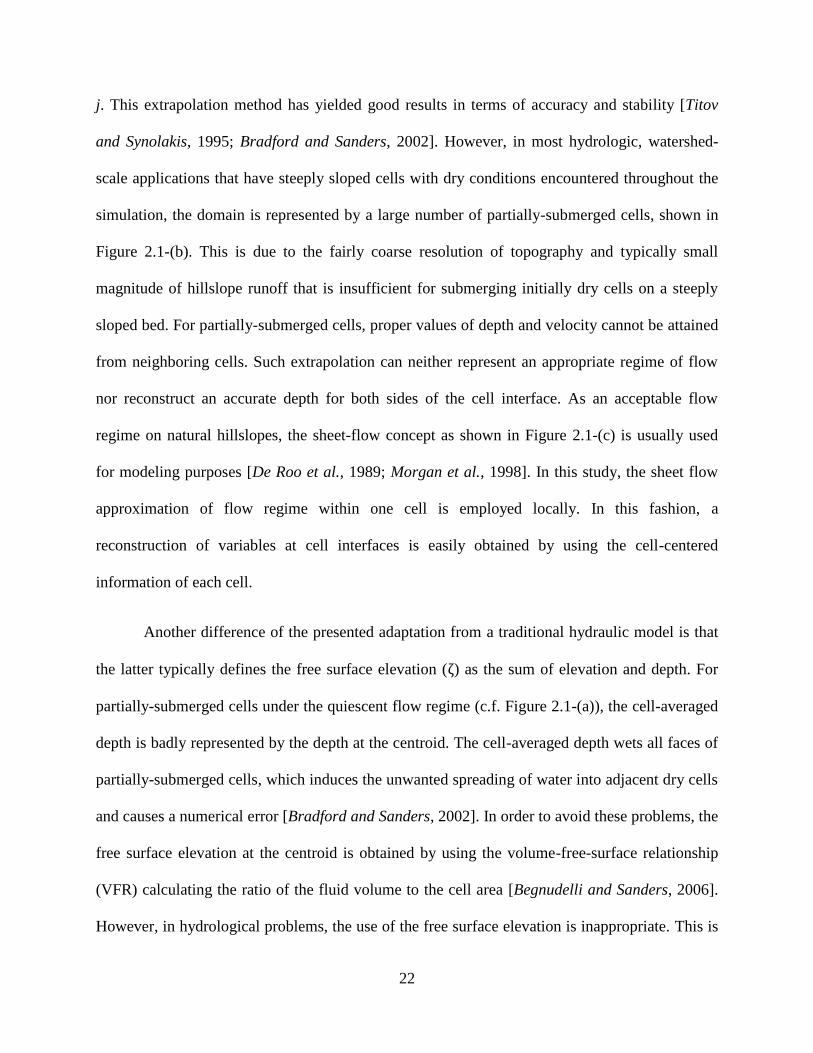
22

j. This extrapolation method has yielded good results in terms of accuracy and stability [Titov

and Synolakis, 1995; Bradford and Sanders, 2002]. However, in most hydrologic, watershed-

scale applications that have steeply sloped cells with dry conditions encountered throughout the

simulation, the domain is represented by a large number of partially-submerged cells, shown in

Figure 2.1-(b). This is due to the fairly coarse resolution of topography and typically small

magnitude of hillslope runoff that is insufficient for submerging initially dry cells on a steeply

sloped bed. For partially-submerged cells, proper values of depth and velocity cannot be attained

from neighboring cells. Such extrapolation can neither represent an appropriate regime of flow

nor reconstruct an accurate depth for both sides of the cell interface. As an acceptable flow

regime on natural hillslopes, the sheet-flow concept as shown in Figure 2.1-(c) is usually used

for modeling purposes [De Roo et al., 1989; Morgan et al., 1998]. In this study, the sheet flow

approximation of flow regime within one cell is employed locally. In this fashion, a

reconstruction of variables at cell interfaces is easily obtained by using the cell-centered

information of each cell.

Another difference of the presented adaptation from a traditional hydraulic model is that

the latter typically defines the free surface elevation ( ) as the sum of elevation and depth. For

partially-submerged cells under the quiescent flow regime (c.f. Figure 2.1-(a)), the cell-averaged

depth is badly represented by the depth at the centroid. The cell-averaged depth wets all faces of

partially-submerged cells, which induces the unwanted spreading of water into adjacent dry cells

and causes a numerical error [Bradford and Sanders, 2002]. In order to avoid these problems, the

free surface elevation at the centroid is obtained by using the volume-free-surface relationship

(VFR) calculating the ratio of the fluid volume to the cell area [Begnudelli and Sanders, 2006].

However, in hydrological problems, the use of the free surface elevation is inappropriate. This is

23

because the free surface elevation in partially-submerged cells is nearly always smaller than the

bed elevation of cell interfaces, and thus, their corresponding flow depths at interfaces are set to

zero. For example, on the left side of each cell interface, the free surface elevation is less than the

bed elevation at the interface, so that its flow depth has a zero value, as shown in Figure 2.1-(b).

Fluxes cannot be properly calculated in such cells with this type of representation. On the other

hand, the sheet flow approximation does not need to perform an additional calculation of the free

surface elevation in the cell interfaces. Cell depths at cell interfaces are attained as flow depths at

the centroid, shown in Figure 2.1-(c).

One of the consequences of the original OFM extrapolation or free surface elevation

estimation of partially-submerged cells in overland flow is the development of a “no-flow

phenomenon”. This refers to a situation when runoff is stored within a cell without the possibility

to flow out. So, the generated runoff fills up the cell until it becomes fully inundated, i.e. “wet”,

according to the accepted definition. At this time, the momentum flux is computed and water

starts flowing to a downstream cell. Note that this numerical problem is very critical in domains

characterized by high bed slopes and low flow conditions (e.g., hillslope areas of the watershed),

where most of the cells correspond to partially-submerged cells. On the other hand, we found

that the local sheet flow approximation using the depth at the cell center instead of free surface

elevations allows one to avoid all of the aforementioned problems.

2.2.4 Information exchange between the hydrologic and hydrodynamic models

This work couples the hydrologic and hydrodynamic models described previously by

using a built-in mapping procedure to exchange information between the computational

24

architectures of the two models. The mapping procedure is needed because tRIBS calculates

physical processes such as interception, infiltration, evapotranspiration as well as runoff, in

elements using the dual diagram of the Triangulated Irregular Network (TIN) - the Voronoi

Polygon Network (VPN) [Ivanov et al., 2004a]. The OFM model computes the flow variables,

including the water depth and velocities, using the TIN [Begnudelli and Sanders, 2006]. The

VPN-based variables obtained after taking into account physical hydrologic processes must be

transferred to the triangle-based variables that will be used in the hydrodynamic model. To do

that, it is assumed that the VPN-based quantities are uniformly distributed inside each Voronoi

cell. Thus, a triangle-based quantity is calculated by spatially-weighting the hydrologic quantities

using the areal fractions of the three Voronoi polygons that compose any given triangle. In this

way, any exchanged quantity is fully conserved.

Three areal Voronoi fractions in each TIN triangle (see Figure 2.2) are calculated with

the ratio as specified in Eq. (2.1). The triangle-based variable at each TIN triangle is computed

by summing the three values using Eq. (2.2). For example, a transformed variable of runoff is

used as the source term in the continuity equation; this transformation of information plays a

crucial role in integrating the two models. As another example of how the mapping procedure is

used, the spatially-variable Manning coefficient given in vertex-based form can be seamlessly

transferred to the cell-based form through the following mapping procedure

∑(

)

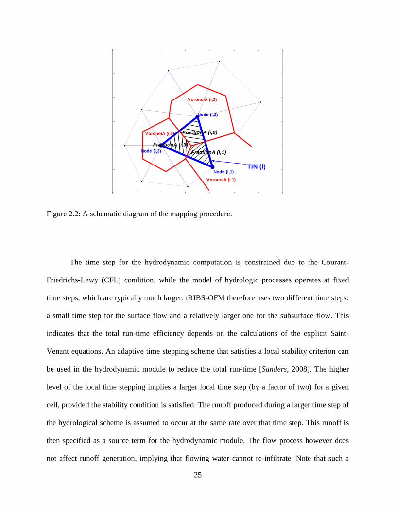
25

Figure 2.2: A schematic diagram of the mapping procedure.

The time step for the hydrodynamic computation is constrained due to the Courant-

Friedrichs-Lewy (CFL) condition, while the model of hydrologic processes operates at fixed

time steps, which are typically much larger. tRIBS-OFM therefore uses two different time steps:

a small time step for the surface flow and a relatively larger one for the subsurface flow. This

indicates that the total run-time efficiency depends on the calculations of the explicit Saint-

Venant equations. An adaptive time stepping scheme that satisfies a local stability criterion can

be used in the hydrodynamic module to reduce the total run-time [Sanders, 2008]. The higher

level of the local time stepping implies a larger local time step (by a factor of two) for a given

cell, provided the stability condition is satisfied. The runoff produced during a larger time step of

the hydrological scheme is assumed to occur at the same rate over that time step. This runoff is

then specified as a source term for the hydrodynamic module. The flow process however does

not affect runoff generation, implying that flowing water cannot re-infiltrate. Note that such a

0 1 2 3 4 5 6 70

1

2

3

4

5

6

FractionA (i,3)

Node (i,3)

Node (i,1)

Node (i,2)

FractionA (i,2)

FractionA (i,1)

TIN (i)

VoronoiA (i,2)

VoronoiA (i,1)

VoronoiA (i,3)

26

one-way exchange of information between modules implies that the coupling between the

surface and subsurface is executed in a “loose” fashion [Sulis et al., 2010].

2.3 OFM verification

The numerical results of the coupled model are compared with an analytical solution,

experimental data, and results obtained by previously developed numerical models. The

analytical solution can be calculated using the kinematic-wave theory only if a domain is of

simple geometry. An impervious soil surface condition is assumed for the verifications, implying

that all precipitation is allowed to become runoff.

2.3.1 One dimensional flow problem over mild-sloped plane

One dimensional flow along an inclined plane with a unit width and a length of 200 m is

simulated. The plane has a bottom slope of 0.001 and a Manning‟s roughness coefficient of 0.03

s/m1/3

. The forcing is a spatially uniform rainfall of 60 mm/hr continuous intensity over the

duration of 1 hour. From the analytical solution of the kinematic-wave problem, the time of

concentration is 31.6 min, the uniform (normal) depth is 0.0316 m, the equilibrium discharge is

, and the kinematic-wave number, (where is the bottom slope,

is the channel length, and is the uniform depth) is 6.25, and the Froude number is 0.188.

The kinematic wave number in this example is small and very close to the threshold value for

of 5.0 above which the kinematic approximation is appropriate [Morris and Woolhiser,

1980]. Also, some internal points have the kinematic-wave number less than 5, meaning that the

dynamic wave method is a better option for the solution. The mesh spacing is 0.5 m, the number

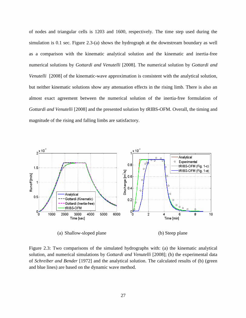
27

of nodes and triangular cells is 1203 and 1600, respectively. The time step used during the

simulation is 0.1 sec. Figure 2.3-(a) shows the hydrograph at the downstream boundary as well

as a comparison with the kinematic analytical solution and the kinematic and inertia-free

numerical solutions by Gottardi and Venutelli [2008]. The numerical solution by Gottardi and

Venutelli [2008] of the kinematic-wave approximation is consistent with the analytical solution,

but neither kinematic solutions show any attenuation effects in the rising limb. There is also an

almost exact agreement between the numerical solution of the inertia-free formulation of

Gottardi and Venutelli [2008] and the presented solution by tRIBS-OFM. Overall, the timing and

magnitude of the rising and falling limbs are satisfactory.

(a) Shallow-sloped plane (b) Steep plane

Figure 2.3: Two comparisons of the simulated hydrographs with: (a) the kinematic analytical

solution, and numerical simulations by Gottardi and Venutelli [2008]; (b) the experimental data

of Schreiber and Bender [1972] and the analytical solution. The calculated results of (b) (green

and blue lines) are based on the dynamic wave method.

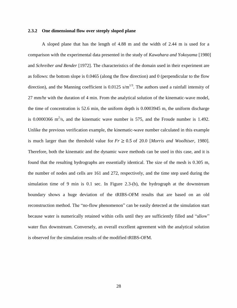
28

2.3.2 One dimensional flow over steeply sloped plane

A sloped plane that has the length of 4.88 m and the width of 2.44 m is used for a

comparison with the experimental data presented in the study of Kawahara and Yokoyama [1980]

and Schreiber and Bender [1972]. The characteristics of the domain used in their experiment are

as follows: the bottom slope is 0.0465 (along the flow direction) and 0 (perpendicular to the flow

direction), and the Manning coefficient is 0.0125 s/m1/3

. The authors used a rainfall intensity of

27 mm/hr with the duration of 4 min. From the analytical solution of the kinematic-wave model,

the time of concentration is 52.6 min, the uniform depth is 0.0003945 m, the uniform discharge

is 0.0000366 m2/s, and the kinematic wave number is 575, and the Froude number is 1.492.

Unlike the previous verification example, the kinematic-wave number calculated in this example

is much larger than the threshold value for of 20.0 [Morris and Woolhiser, 1980].

Therefore, both the kinematic and the dynamic wave methods can be used in this case, and it is

found that the resulting hydrographs are essentially identical. The size of the mesh is 0.305 m,

the number of nodes and cells are 161 and 272, respectively, and the time step used during the

simulation time of 9 min is 0.1 sec. In Figure 2.3-(b), the hydrograph at the downstream

boundary shows a huge deviation of the tRIBS-OFM results that are based on an old

reconstruction method. The “no-flow phenomenon” can be easily detected at the simulation start

because water is numerically retained within cells until they are sufficiently filled and “allow”

water flux downstream. Conversely, an overall excellent agreement with the analytical solution

is observed for the simulation results of the modified tRIBS-OFM.

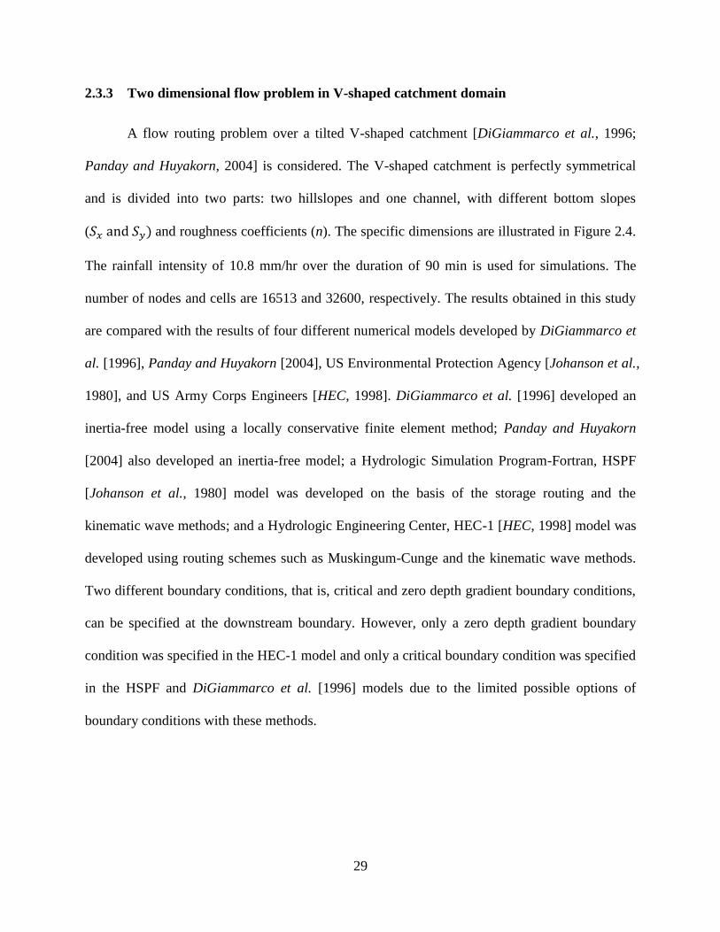
29

2.3.3 Two dimensional flow problem in V-shaped catchment domain

A flow routing problem over a tilted V-shaped catchment [DiGiammarco et al., 1996;

Panday and Huyakorn, 2004] is considered. The V-shaped catchment is perfectly symmetrical

and is divided into two parts: two hillslopes and one channel, with different bottom slopes

( and roughness coefficients (n). The specific dimensions are illustrated in Figure 2.4.

The rainfall intensity of 10.8 mm/hr over the duration of 90 min is used for simulations. The

number of nodes and cells are 16513 and 32600, respectively. The results obtained in this study

are compared with the results of four different numerical models developed by DiGiammarco et

al. [1996], Panday and Huyakorn [2004], US Environmental Protection Agency [Johanson et al.,

1980], and US Army Corps Engineers [HEC, 1998]. DiGiammarco et al. [1996] developed an

inertia-free model using a locally conservative finite element method; Panday and Huyakorn

[2004] also developed an inertia-free model; a Hydrologic Simulation Program-Fortran, HSPF

[Johanson et al., 1980] model was developed on the basis of the storage routing and the

kinematic wave methods; and a Hydrologic Engineering Center, HEC-1 [HEC, 1998] model was

developed using routing schemes such as Muskingum-Cunge and the kinematic wave methods.

Two different boundary conditions, that is, critical and zero depth gradient boundary conditions,

can be specified at the downstream boundary. However, only a zero depth gradient boundary

condition was specified in the HEC-1 model and only a critical boundary condition was specified

in the HSPF and DiGiammarco et al. [1996] models due to the limited possible options of

boundary conditions with these methods.

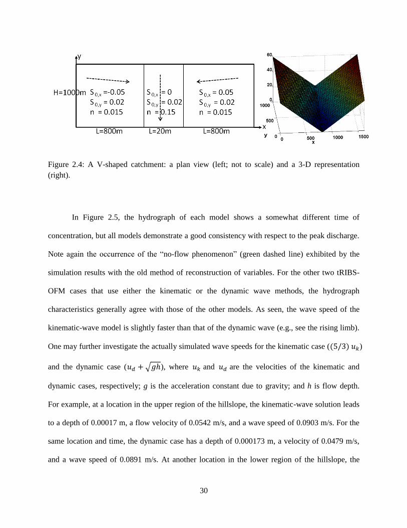
30

Figure 2.4: A V-shaped catchment: a plan view (left; not to scale) and a 3-D representation

(right).

In Figure 2.5, the hydrograph of each model shows a somewhat different time of

concentration, but all models demonstrate a good consistency with respect to the peak discharge.

Note again the occurrence of the “no-flow phenomenon” (green dashed line) exhibited by the

simulation results with the old method of reconstruction of variables. For the other two tRIBS-

OFM cases that use either the kinematic or the dynamic wave methods, the hydrograph

characteristics generally agree with those of the other models. As seen, the wave speed of the

kinematic-wave model is slightly faster than that of the dynamic wave (e.g., see the rising limb).

One may further investigate the actually simulated wave speeds for the kinematic case ( )

and the dynamic case ( √ ), where and are the velocities of the kinematic and

dynamic cases, respectively; g is the acceleration constant due to gravity; and h is flow depth.

For example, at a location in the upper region of the hillslope, the kinematic-wave solution leads

to a depth of 0.00017 m, a flow velocity of 0.0542 m/s, and a wave speed of 0.0903 m/s. For the

same location and time, the dynamic case has a depth of 0.000173 m, a velocity of 0.0479 m/s,

and a wave speed of 0.0891 m/s. At another location in the lower region of the hillslope, the

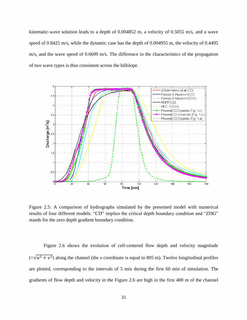
31

kinematic-wave solution leads to a depth of 0.004852 m, a velocity of 0.5055 m/s, and a wave

speed of 0.8425 m/s, while the dynamic case has the depth of 0.004955 m, the velocity of 0.4495

m/s, and the wave speed of 0.6699 m/s. The difference in the characteristics of the propagation

of two wave types is thus consistent across the hillslope.

Figure 2.5: A comparison of hydrographs simulated by the presented model with numerical

results of four different models. “CD” implies the critical depth boundary condition and “ZDG”

stands for the zero depth gradient boundary condition.

Figure 2.6 shows the evolution of cell-centered flow depth and velocity magnitude

(=√ ) along the channel (the x coordinate is equal to 805 m). Twelve longitudinal profiles

are plotted, corresponding to the intervals of 5 min during the first 60 min of simulation. The

gradients of flow depth and velocity in the Figure 2.6 are high in the first 400 m of the channel

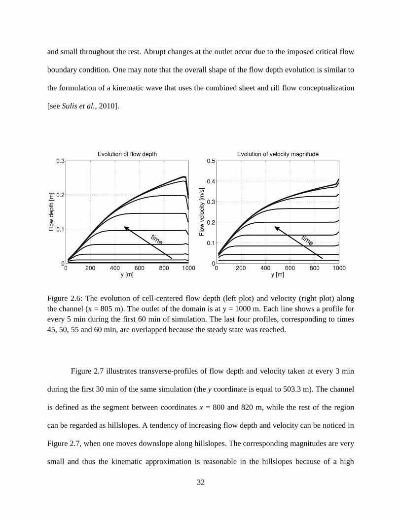
32

and small throughout the rest. Abrupt changes at the outlet occur due to the imposed critical flow

boundary condition. One may note that the overall shape of the flow depth evolution is similar to

the formulation of a kinematic wave that uses the combined sheet and rill flow conceptualization

[see Sulis et al., 2010].

Figure 2.6: The evolution of cell-centered flow depth (left plot) and velocity (right plot) along

the channel (x = 805 m). The outlet of the domain is at y = 1000 m. Each line shows a profile for

every 5 min during the first 60 min of simulation. The last four profiles, corresponding to times

45, 50, 55 and 60 min, are overlapped because the steady state was reached.

Figure 2.7 illustrates transverse-profiles of flow depth and velocity taken at every 3 min

during the first 30 min of the same simulation (the y coordinate is equal to 503.3 m). The channel

is defined as the segment between coordinates x = 800 and 820 m, while the rest of the region

can be regarded as hillslopes. A tendency of increasing flow depth and velocity can be noticed in

Figure 2.7, when one moves downslope along hillslopes. The corresponding magnitudes are very

small and thus the kinematic approximation is reasonable in the hillslopes because of a high

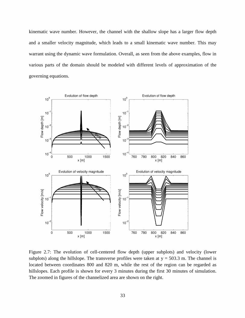
33

kinematic wave number. However, the channel with the shallow slope has a larger flow depth

and a smaller velocity magnitude, which leads to a small kinematic wave number. This may

warrant using the dynamic wave formulation. Overall, as seen from the above examples, flow in

various parts of the domain should be modeled with different levels of approximation of the

governing equations.

Figure 2.7: The evolution of cell-centered flow depth (upper subplots) and velocity (lower

subplots) along the hillslope. The transverse profiles were taken at y = 503.3 m. The channel is

located between coordinates 800 and 820 m, while the rest of the region can be regarded as

hillslopes. Each profile is shown for every 3 minutes during the first 30 minutes of simulation.

The zoomed in figures of the channelized area are shown on the right.

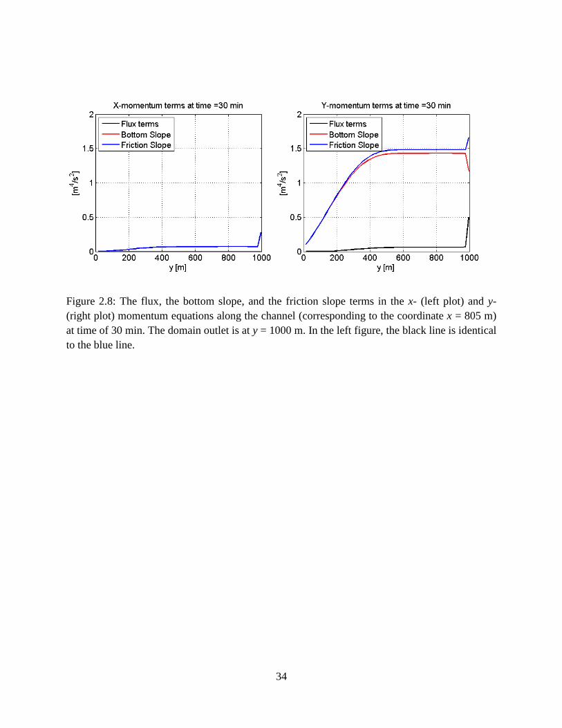
34

Figure 2.8: The flux, the bottom slope, and the friction slope terms in the x- (left plot) and y-

(right plot) momentum equations along the channel (corresponding to the coordinate x = 805 m)

at time of 30 min. The domain outlet is at y = 1000 m. In the left figure, the black line is identical

to the blue line.

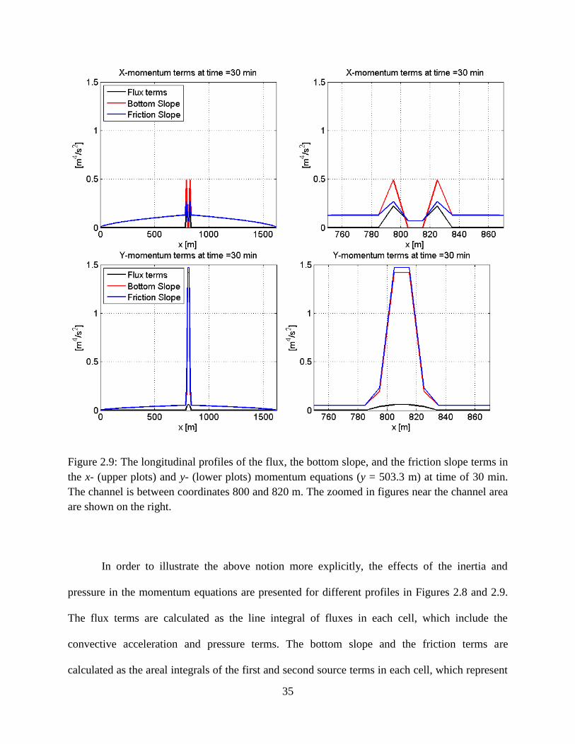
35

Figure 2.9: The longitudinal profiles of the flux, the bottom slope, and the friction slope terms in

the x- (upper plots) and y- (lower plots) momentum equations (y = 503.3 m) at time of 30 min.

The channel is between coordinates 800 and 820 m. The zoomed in figures near the channel area

are shown on the right.

In order to illustrate the above notion more explicitly, the effects of the inertia and

pressure in the momentum equations are presented for different profiles in Figures 2.8 and 2.9.

The flux terms are calculated as the line integral of fluxes in each cell, which include the

convective acceleration and pressure terms. The bottom slope and the friction terms are

calculated as the areal integrals of the first and second source terms in each cell, which represent

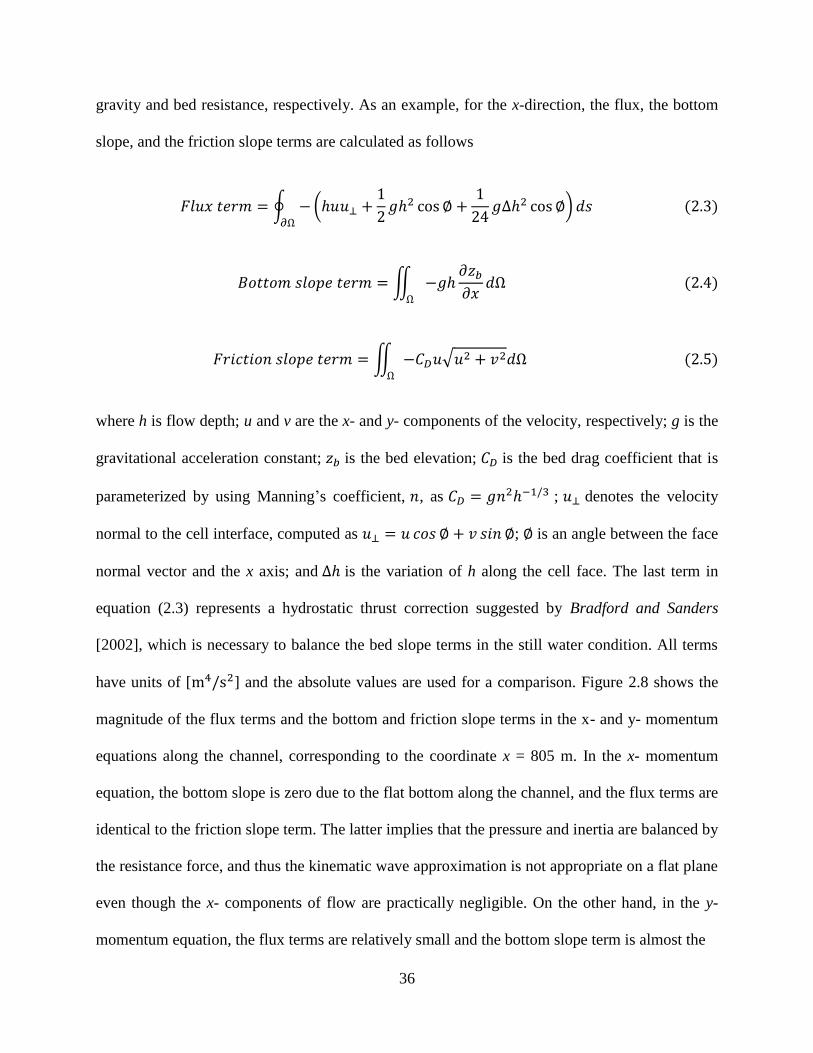
36

gravity and bed resistance, respectively. As an example, for the x-direction, the flux, the bottom

slope, and the friction slope terms are calculated as follows

∮ (

)

∬

∬ √

where h is flow depth; u and v are the x- and y- components of the velocity, respectively; g is the

gravitational acceleration constant; is the bed elevation; is the bed drag coefficient that is

parameterized by using Manning‟s coefficient, , as ; denotes the velocity

normal to the cell interface, computed as ; is an angle between the face

normal vector and the x axis; and is the variation of h along the cell face. The last term in

equation (2.3) represents a hydrostatic thrust correction suggested by Bradford and Sanders

[2002], which is necessary to balance the bed slope terms in the still water condition. All terms

have units of [ ] and the absolute values are used for a comparison. Figure 2.8 shows the

magnitude of the flux terms and the bottom and friction slope terms in the x- and y- momentum

equations along the channel, corresponding to the coordinate x = 805 m. In the x- momentum

equation, the bottom slope is zero due to the flat bottom along the channel, and the flux terms are

identical to the friction slope term. The latter implies that the pressure and inertia are balanced by

the resistance force, and thus the kinematic wave approximation is not appropriate on a flat plane

even though the x- components of flow are practically negligible. On the other hand, in the y-

momentum equation, the flux terms are relatively small and the bottom slope term is almost the

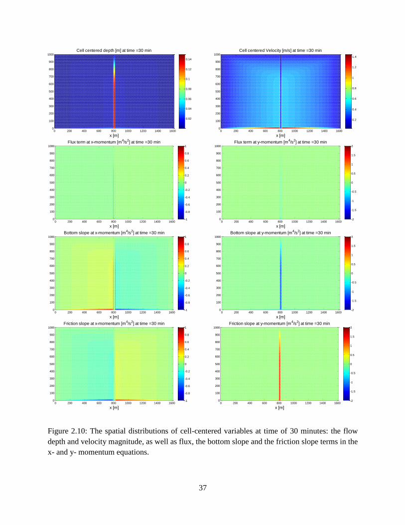
37

Figure 2.10: The spatial distributions of cell-centered variables at time of 30 minutes: the flow

depth and velocity magnitude, as well as flux, the bottom slope and the friction slope terms in the

x- and y- momentum equations.

0 200 400 600 800 1000 1200 1400 16000

100

200

300

400

500

600

700

800

900

1000

x [m]

y [m

]

Cell centered depth [m] at time =30 min

0.02

0.04

0.06

0.08

0.1

0.12

0.14

0 200 400 600 800 1000 1200 1400 16000

100

200

300

400

500

600

700

800

900

1000

x [m]

y [m

]

Cell centered Velocity [m/s] at time =30 min

0.2

0.4

0.6

0.8

1

1.2

1.4

0 200 400 600 800 1000 1200 1400 16000

100

200

300

400

500

600

700

800

900

1000

x [m]

y [m

]

Flux term at x-momentum [m4/s

2] at time =30 min

-1

-0.8

-0.6

-0.4

-0.2

0

0.2

0.4

0.6

0.8

1

0 200 400 600 800 1000 1200 1400 16000

100

200

300

400

500

600

700

800

900

1000

x [m]

y [m

]

Flux term at y-momentum [m4/s

2] at time =30 min

-2

-1.5

-1

-0.5

0

0.5

1

1.5

2

0 200 400 600 800 1000 1200 1400 16000

100

200

300

400

500

600

700

800

900

1000

x [m]

y [m

]

Bottom slope at x-momentum [m4/s

2] at time =30 min

-1

-0.8

-0.6

-0.4

-0.2

0

0.2

0.4

0.6

0.8

1

0 200 400 600 800 1000 1200 1400 16000

100

200

300

400

500

600

700

800

900

1000

x [m]

y [m

]

Bottom slope at y-momentum [m4/s

2] at time =30 min

-2

-1.5

-1

-0.5

0

0.5

1

1.5

2

0 200 400 600 800 1000 1200 1400 16000

100

200

300

400

500

600

700

800

900

1000

x [m]

y [m

]

Friction slope at x-momentum [m4/s

2] at time =30 min

-1

-0.8

-0.6

-0.4

-0.2

0

0.2

0.4

0.6

0.8

1

0 200 400 600 800 1000 1200 1400 16000

100

200

300

400

500

600

700

800

900

1000

x [m]

y [m

]

Friction slope at y-momentum [m4/s

2] at time =30 min

-2

-1.5

-1

-0.5

0

0.5

1

1.5

2

38

same with the friction slope term. Still, one can expect small errors (less than 5 %) to occur if the

kinematic wave method is used for this flow situation.

The importance of the flux terms in the channel area is highlighted in Figure 2.9, which

provides longitudinal profiles (i.e., along the x- axis). The flux terms are nearly zero, and the two

other terms are almost the same in the hillslope region. Thus, the kinematic wave approximation

for both directions is a natural simplification. However, in the transitional area between the

hillslope and the channel (e.g., 780 < x < 800 m), the flux terms become significant and their

magnitudes are of the same order as the other terms. Consequently, the “dynamic” effects are

generally minor for a simple hillslope but should be considered for a consistent description of the

flow situation where topography is characterized by flat slopes or where vastly varying slopes

exist.

The spatial distributions of cell-centered variables such as the flow depth, the velocity,

and the terms of the momentum equation (in both the x- and y- directions) at time equal to 30

min are shown in Figure 2.10. The figure allows one to appreciate the spatial variability of flow

situations that can be described with various degrees of approximation of the Saint-Venant

equations. It illustrates the differences between the channel and hillslopes as well as the

symmetry of simulated variables for both hillslopes. The flow depth is less than few centimeters

in the hillslopes, but it is larger by one order of magnitude in the channel. The flow velocity in

the hillslopes is higher than that in the channel and it is generally less than 0.5 m/s. In terms of

the spatial distribution of the momentum terms, the same conclusions can be made, i.e., the

relative importance of the inertia and pressure terms is not very high and the kinematic

approximation is appropriate for the hillslope areas. However, the influence of inertia and

pressure increases when an abrupt change of topography occurs near the channel. The preceding

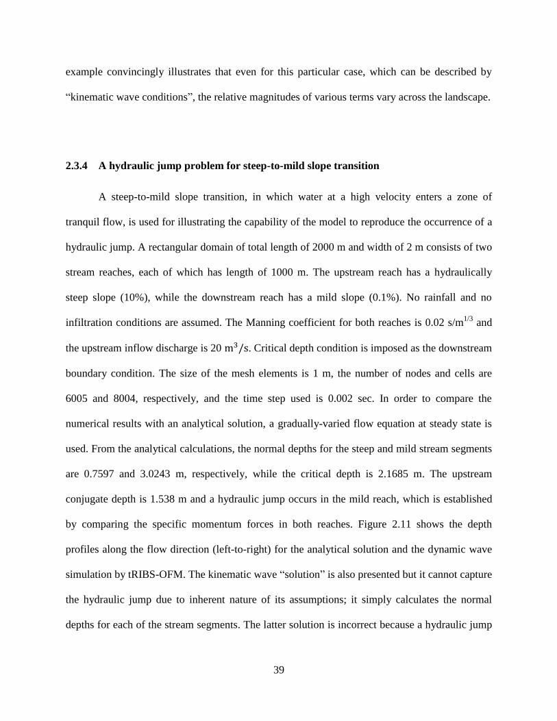
39

example convincingly illustrates that even for this particular case, which can be described by

“kinematic wave conditions”, the relative magnitudes of various terms vary across the landscape.

2.3.4 A hydraulic jump problem for steep-to-mild slope transition

A steep-to-mild slope transition, in which water at a high velocity enters a zone of

tranquil flow, is used for illustrating the capability of the model to reproduce the occurrence of a

hydraulic jump. A rectangular domain of total length of 2000 m and width of 2 m consists of two

stream reaches, each of which has length of 1000 m. The upstream reach has a hydraulically

steep slope (10%), while the downstream reach has a mild slope (0.1%). No rainfall and no

infiltration conditions are assumed. The Manning coefficient for both reaches is 0.02 s/m1/3

and

the upstream inflow discharge is 20 . Critical depth condition is imposed as the downstream

boundary condition. The size of the mesh elements is 1 m, the number of nodes and cells are

6005 and 8004, respectively, and the time step used is 0.002 sec. In order to compare the

numerical results with an analytical solution, a gradually-varied flow equation at steady state is

used. From the analytical calculations, the normal depths for the steep and mild stream segments

are 0.7597 and 3.0243 m, respectively, while the critical depth is 2.1685 m. The upstream

conjugate depth is 1.538 m and a hydraulic jump occurs in the mild reach, which is established

by comparing the specific momentum forces in both reaches. Figure 2.11 shows the depth

profiles along the flow direction (left-to-right) for the analytical solution and the dynamic wave

simulation by tRIBS-OFM. The kinematic wave “solution” is also presented but it cannot capture

the hydraulic jump due to inherent nature of its assumptions; it simply calculates the normal

depths for each of the stream segments. The latter solution is incorrect because a hydraulic jump

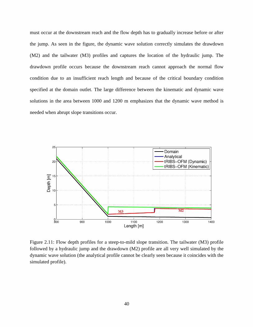
40

must occur at the downstream reach and the flow depth has to gradually increase before or after

the jump. As seen in the figure, the dynamic wave solution correctly simulates the drawdown

(M2) and the tailwater (M3) profiles and captures the location of the hydraulic jump. The

drawdown profile occurs because the downstream reach cannot approach the normal flow

condition due to an insufficient reach length and because of the critical boundary condition

specified at the domain outlet. The large difference between the kinematic and dynamic wave

solutions in the area between 1000 and 1200 m emphasizes that the dynamic wave method is

needed when abrupt slope transitions occur.

Figure 2.11: Flow depth profiles for a steep-to-mild slope transition. The tailwater (M3) profile

followed by a hydraulic jump and the drawdown (M2) profile are all very well simulated by the

dynamic wave solution (the analytical profile cannot be clearly seen because it coincides with the

simulated profile).

41

2.4 Model application

2.4.1 Model application to a synthetic watershed

The presented model shows a good performance when compared to other model results

for the cases of simple domain topography and rainfall input. In order to investigate the rainfall-

runoff phenomenon under more complicated conditions, a synthetic domain is used with three

different inputs of precipitation and four mesh types. The synthetic domain selected for the

simulations represents a wide range of geometric characteristics, such as slope magnitudes and

flow drainage directions. The three different inputs of precipitation correspond to uniform

intensities of 10, 50 and 100 mm/hr. The domain is 2 km 2 km and the dimension of a typical

TIN element in the coarsest mesh is about 30 m 40 m (the elements are of triangular shape).

Figure 2.12-(a) and 2.12-(d) show the three-dimensional topographic representations of the

coarser and finer mesh illustrating both valleys and hillslopes. The four different mesh types

shown in Figure 2.12-(a) to 2.12-(d) are used to evaluate the sensitivity of the hydrograph

simulation to mesh resolution. The domain shown in Figure 2.12-(a) has a uniform coarse

resolution, where each cell has an area of 600 m2. The domain shown in Figure 2.12-(d) is

resolved at a finer scale, with cells that are 9 times smaller. The domains shown in Figure 2.12-(b)

and 2.12-(c) have nested regions resolved at a finer scale (same as Figure 2.12-(d)). This mesh

generation is performed by refining the region where the flow concentration is anticipated

according to the convergence of surface contributing areas. For example, Figure 2.12-(b) and

2.12-(c) are refined in the region where the surface contributing area of each Voronoi cell

(defined using the steepest drainage direction approach, e.g., Ivanov et al. [2004a]) is greater

than 10 and 1 percent of the total contributing area of the domain, respectively. The total

contributing area at the outlet of all domains is 4 km2. In total, 2601, 4717, 7918 and 22801

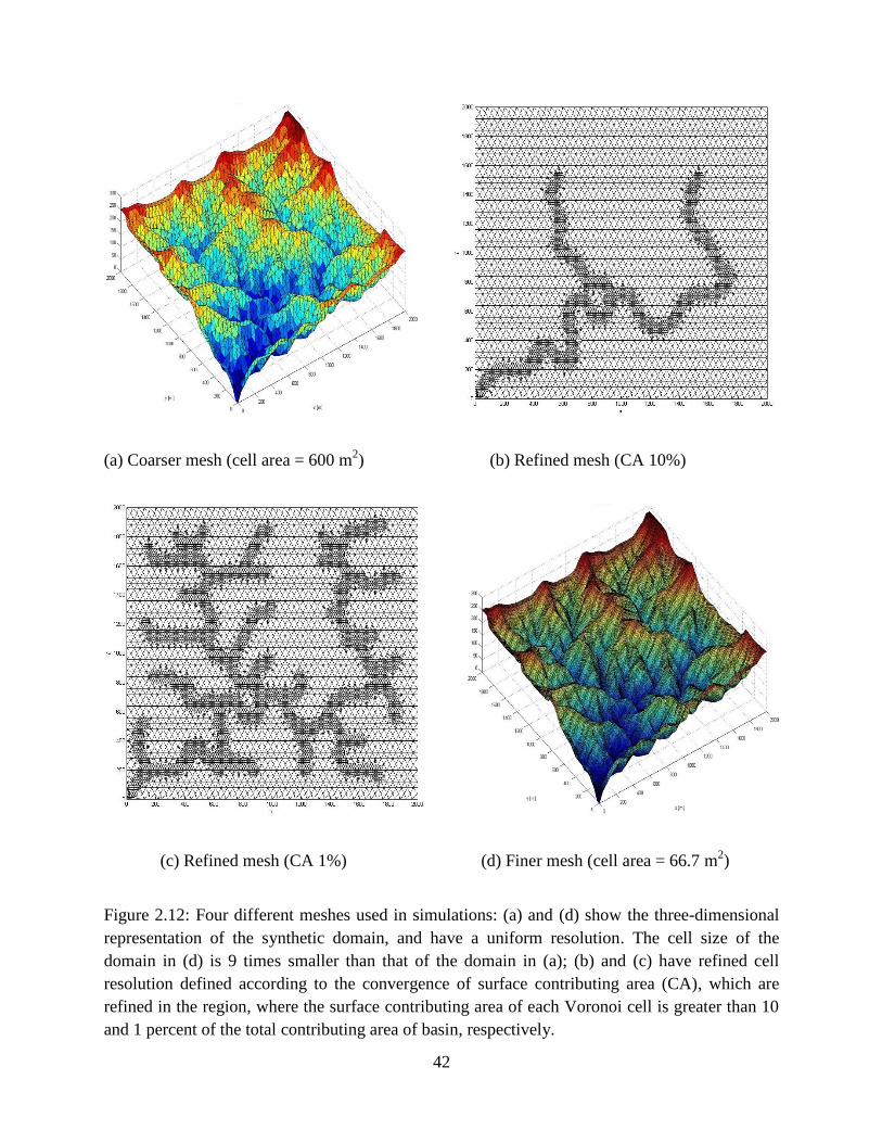
42

(a) Coarser mesh (cell area = 600 m2) (b) Refined mesh (CA 10%)

(c) Refined mesh (CA 1%) (d) Finer mesh (cell area = 66.7 m2)

Figure 2.12: Four different meshes used in simulations: (a) and (d) show the three-dimensional

representation of the synthetic domain, and have a uniform resolution. The cell size of the

domain in (d) is 9 times smaller than that of the domain in (a); (b) and (c) have refined cell

resolution defined according to the convergence of surface contributing area (CA), which are

refined in the region, where the surface contributing area of each Voronoi cell is greater than 10

and 1 percent of the total contributing area of basin, respectively.

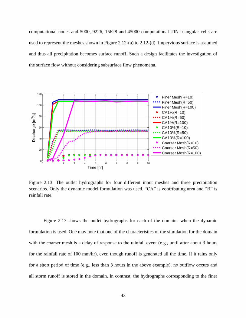
43

computational nodes and 5000, 9226, 15628 and 45000 computational TIN triangular cells are

used to represent the meshes shown in Figure 2.12-(a) to 2.12-(d). Impervious surface is assumed

and thus all precipitation becomes surface runoff. Such a design facilitates the investigation of

the surface flow without considering subsurface flow phenomena.

Figure 2.13: The outlet hydrographs for four different input meshes and three precipitation

scenarios. Only the dynamic model formulation was used. “CA” is contributing area and “R” is

rainfall rate.

Figure 2.13 shows the outlet hydrographs for each of the domains when the dynamic

formulation is used. One may note that one of the characteristics of the simulation for the domain

with the coarser mesh is a delay of response to the rainfall event (e.g., until after about 3 hours

for the rainfall rate of 100 mm/hr), even though runoff is generated all the time. If it rains only

for a short period of time (e.g., less than 3 hours in the above example), no outflow occurs and

all storm runoff is stored in the domain. In contrast, the hydrographs corresponding to the finer

0 1 2 3 4 5 6 7 8 9 100

20

40

60

80

100

120

Time [hr]

Dis

ch

arg

e [m

3/s

]

Finer Mesh(R=10)

Finer Mesh(R=50)

Finer Mesh(R=100)

CA1%(R=10)

CA1%(R=50)

CA1%(R=100)

CA10%(R=10)

CA10%(R=50)

CA10%(R=100)

Coarser Mesh(R=10)

Coarser Mesh(R=50)

Coarser Mesh(R=100)

44

mesh cases exhibit non-zero outflow at the outlet shortly after 1.5 hours. All domains show

similar values of peak discharge after a steady state is achieved because the same magnitude of

precipitation is used (the minor difference in magnitudes is due to slightly different total runoff

production because the runoff outside of Voronoi cells located along the boundaries is assumed

to be zero). For the lower rate of precipitation (see also Figure 2.13), a similar effect of the

dependence of the time of concentration on mesh resolution can be observed. These results imply

that the model behavior is resolution-dependent.

In previous research by Begnudelli and Sanders [2007], Yu and Lane [2006] and Sulis et

al. [2011], similar results were achieved, in terms of the effect of grid resolution on the flow.

Begnudelli and Sanders [2007] applied their model to simulate the St. Francis dam break

problem with different Manning‟s coefficients and with different mesh resolutions. According to

their results, an increase in the mesh resolution had a significant effect on the flood behavior: the

time of concentration was smaller for a finer mesh than for a coarser mesh due to the higher

speed of the flood in the former case. Begnudelli and Sanders [2007] explained this phenomenon

by stating that “a poorly resolved grid behaves similarly to a grid with an unrealistically large

resistance parameter”.

To provide a deeper insight for such an effect, slope characteristics of four mesh types

were examined. In the channel network, slopes are typically small, with magnitudes lower than 1

degree. In the hillslope, slopes can be very steep, larger than 40 degrees. Such a high slope

magnitude results in a significant elevation difference among the triangle vertices, particularly

for a coarse mesh. Therefore, using a refined mesh near the channel can contribute to different

delineations of channel and floodplain. A coarser mesh represents a much wider channel width

than a mesh with a finer resolution. The implication is that a wider channel width influences the

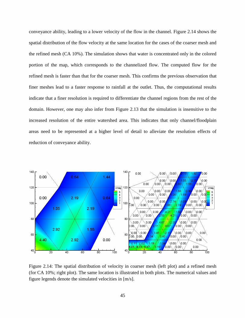
45

conveyance ability, leading to a lower velocity of the flow in the channel. Figure 2.14 shows the

spatial distribution of the flow velocity at the same location for the cases of the coarser mesh and

the refined mesh (CA 10%). The simulation shows that water is concentrated only in the colored

portion of the map, which corresponds to the channelized flow. The computed flow for the

refined mesh is faster than that for the coarser mesh. This confirms the previous observation that

finer meshes lead to a faster response to rainfall at the outlet. Thus, the computational results

indicate that a finer resolution is required to differentiate the channel regions from the rest of the

domain. However, one may also infer from Figure 2.13 that the simulation is insensitive to the

increased resolution of the entire watershed area. This indicates that only channel/floodplain

areas need to be represented at a higher level of detail to alleviate the resolution effects of

reduction of conveyance ability.

Figure 2.14: The spatial distribution of velocity in coarser mesh (left plot) and a refined mesh

(for CA 10%; right plot). The same location is illustrated in both plots. The numerical values and

figure legends denote the simulated velocities in [m/s].

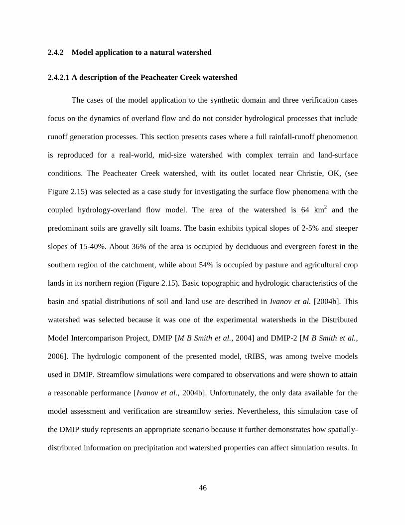
46

2.4.2 Model application to a natural watershed

2.4.2.1 A description of the Peacheater Creek watershed

The cases of the model application to the synthetic domain and three verification cases

focus on the dynamics of overland flow and do not consider hydrological processes that include

runoff generation processes. This section presents cases where a full rainfall-runoff phenomenon

is reproduced for a real-world, mid-size watershed with complex terrain and land-surface

conditions. The Peacheater Creek watershed, with its outlet located near Christie, OK, (see

Figure 2.15) was selected as a case study for investigating the surface flow phenomena with the

coupled hydrology-overland flow model. The area of the watershed is 64 km2 and the

predominant soils are gravelly silt loams. The basin exhibits typical slopes of 2-5% and steeper

slopes of 15-40%. About 36% of the area is occupied by deciduous and evergreen forest in the

southern region of the catchment, while about 54% is occupied by pasture and agricultural crop

lands in its northern region (Figure 2.15). Basic topographic and hydrologic characteristics of the

basin and spatial distributions of soil and land use are described in Ivanov et al. [2004b]. This

watershed was selected because it was one of the experimental watersheds in the Distributed

Model Intercomparison Project, DMIP [M B Smith et al., 2004] and DMIP-2 [M B Smith et al.,

2006]. The hydrologic component of the presented model, tRIBS, was among twelve models

used in DMIP. Streamflow simulations were compared to observations and were shown to attain

a reasonable performance [Ivanov et al., 2004b]. Unfortunately, the only data available for the

model assessment and verification are streamflow series. Nevertheless, this simulation case of

the DMIP study represents an appropriate scenario because it further demonstrates how spatially-

distributed information on precipitation and watershed properties can affect simulation results. In

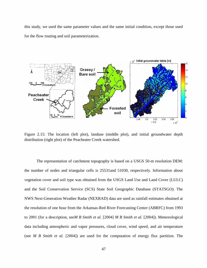
47

this study, we used the same parameter values and the same initial condition, except those used

for the flow routing and soil parameterization.

Figure 2.15: The location (left plot), landuse (middle plot), and initial groundwater depth

distribution (right plot) of the Peacheater Creek watershed.

The representation of catchment topography is based on a USGS 50-m resolution DEM:

the number of nodes and triangular cells is 25531and 51030, respectively. Information about

vegetation cover and soil type was obtained from the USGS Land Use and Land Cover (LULC)

and the Soil Conservation Service (SCS) State Soil Geographic Database (STATSGO). The

NWS Next-Generation Weather Radar (NEXRAD) data are used as rainfall estimates obtained at

the resolution of one hour from the Arkansas-Red River Forecasting Center (ABRFC) from 1993

to 2001 (for a description, seeM B Smith et al. [2004] M B Smith et al. [2004]). Meteorological

data including atmospheric and vapor pressures, cloud cover, wind speed, and air temperature

(see M B Smith et al. [2004]) are used for the computation of energy flux partition. The

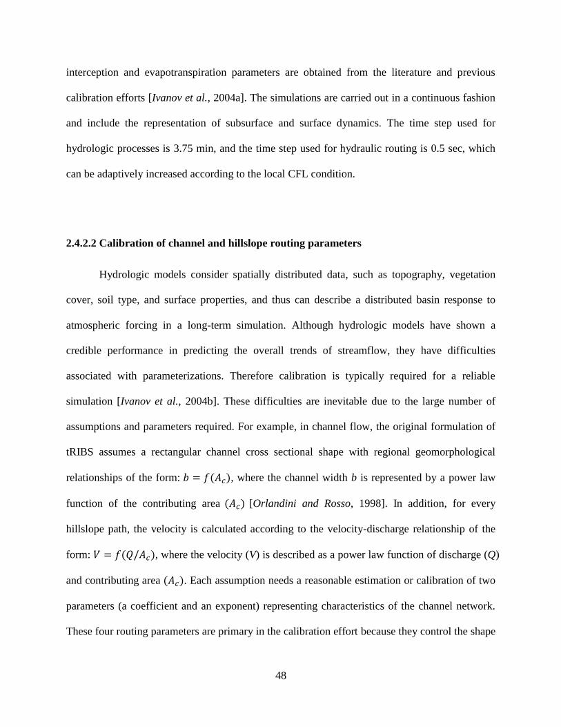
48

interception and evapotranspiration parameters are obtained from the literature and previous

calibration efforts [Ivanov et al., 2004a]. The simulations are carried out in a continuous fashion

and include the representation of subsurface and surface dynamics. The time step used for

hydrologic processes is 3.75 min, and the time step used for hydraulic routing is 0.5 sec, which

can be adaptively increased according to the local CFL condition.

2.4.2.2 Calibration of channel and hillslope routing parameters

Hydrologic models consider spatially distributed data, such as topography, vegetation

cover, soil type, and surface properties, and thus can describe a distributed basin response to

atmospheric forcing in a long-term simulation. Although hydrologic models have shown a

credible performance in predicting the overall trends of streamflow, they have difficulties

associated with parameterizations. Therefore calibration is typically required for a reliable

simulation [Ivanov et al., 2004b]. These difficulties are inevitable due to the large number of

assumptions and parameters required. For example, in channel flow, the original formulation of

tRIBS assumes a rectangular channel cross sectional shape with regional geomorphological

relationships of the form: , where the channel width b is represented by a power law

function of the contributing area [Orlandini and Rosso, 1998]. In addition, for every

hillslope path, the velocity is calculated according to the velocity-discharge relationship of the

form: , where the velocity (V) is described as a power law function of discharge (Q)

and contributing area . Each assumption needs a reasonable estimation or calibration of two

parameters (a coefficient and an exponent) representing characteristics of the channel network.

These four routing parameters are primary in the calibration effort because they control the shape

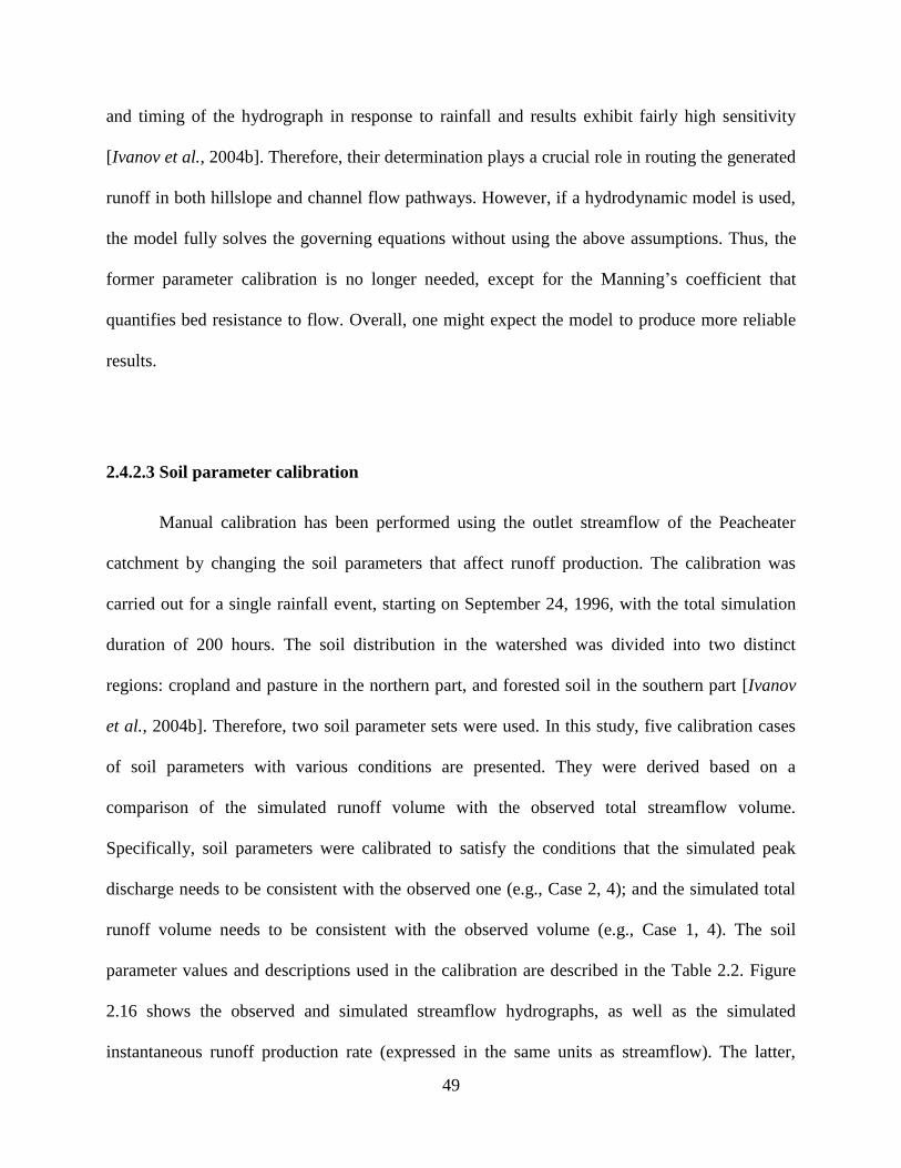
49

and timing of the hydrograph in response to rainfall and results exhibit fairly high sensitivity

[Ivanov et al., 2004b]. Therefore, their determination plays a crucial role in routing the generated

runoff in both hillslope and channel flow pathways. However, if a hydrodynamic model is used,

the model fully solves the governing equations without using the above assumptions. Thus, the

former parameter calibration is no longer needed, except for the Manning‟s coefficient that

quantifies bed resistance to flow. Overall, one might expect the model to produce more reliable

results.

2.4.2.3 Soil parameter calibration

Manual calibration has been performed using the outlet streamflow of the Peacheater

catchment by changing the soil parameters that affect runoff production. The calibration was

carried out for a single rainfall event, starting on September 24, 1996, with the total simulation

duration of 200 hours. The soil distribution in the watershed was divided into two distinct

regions: cropland and pasture in the northern part, and forested soil in the southern part [Ivanov

et al., 2004b]. Therefore, two soil parameter sets were used. In this study, five calibration cases

of soil parameters with various conditions are presented. They were derived based on a

comparison of the simulated runoff volume with the observed total streamflow volume.

Specifically, soil parameters were calibrated to satisfy the conditions that the simulated peak

discharge needs to be consistent with the observed one (e.g., Case 2, 4); and the simulated total

runoff volume needs to be consistent with the observed volume (e.g., Case 1, 4). The soil

parameter values and descriptions used in the calibration are described in the Table 2.2. Figure

2.16 shows the observed and simulated streamflow hydrographs, as well as the simulated

instantaneous runoff production rate (expressed in the same units as streamflow). The latter,

50

influenced by soil parameters, is an output of hydrologic processes and used as an input to the

model of hydrodynamic routing. Overall, small discrepancies between hydrographs can be

detected, as shown in Figure 2.16. But for Cases 2 and 4, the peak discharge agrees well with the

observed value and hydrographs exhibit a similar shape. Based on various error indices, Case 4

shows the best fit with the observed data (See Table 2.4).

Figure 2.16: The effect of soil parameters on streamflow; mean areal precipitation (upper and

right axis) and hydrographs (lower and left axis) of the observed discharge and simulated runoff

and discharge. The illustrated cases have the same, spatially two different values of Manning‟s

coefficient (See Table 2.3 and 2.4).

51

Figure 2.17: The effect of the Manning‟s coefficient scenario on streamflow simulation. The

mean areal precipitation (upper and right axis) and observed (black line) and simulated (dash

lines) hydrographs are illustrated. The cases shown have the same soil parameters as the Case 4

of the soil scenarios.

2.4.2.4 Parameterization of the hydrodynamic routing model

The Saint-Venant equations are fundamental physics-based equations describing flow

motion using mass and momentum conservation laws. Therefore, all parameters used in the

equations can be theoretically measurable. For example, many researchers have parameterized

the bed drag coefficient ( ) by using Manning‟s, Chezy‟s, or Darcy-Weisbach coefficients, to

calculate the friction terms. These coefficients can be obtained by measuring the roughness

height over the flow surface, but it is quite impossible to get measured data for every

computational element due to the spatial heterogeneity. As an alternative approach to this

problem, calibration of the roughness coefficient can be performed in the hydrodynamic routing

problem. In this study, two different cases were used due to insufficient information about the

roughness in this watershed. First, a spatially uniform Manning coefficient and second, two

values of the coefficient corresponding to the hillslope and channel flow paths were used (See

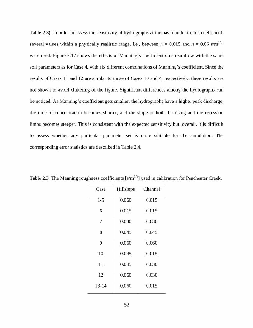
52

Table 2.3). In order to assess the sensitivity of hydrographs at the basin outlet to this coefficient,

several values within a physically realistic range, i.e., between n = 0.015 and n = 0.06 s/m1/3

,

were used. Figure 2.17 shows the effects of Manning‟s coefficient on streamflow with the same

soil parameters as for Case 4, with six different combinations of Manning‟s coefficient. Since the

results of Cases 11 and 12 are similar to those of Cases 10 and 4, respectively, these results are

not shown to avoid cluttering of the figure. Significant differences among the hydrographs can

be noticed. As Manning‟s coefficient gets smaller, the hydrographs have a higher peak discharge,

the time of concentration becomes shorter, and the slope of both the rising and the recession

limbs becomes steeper. This is consistent with the expected sensitivity but, overall, it is difficult

to assess whether any particular parameter set is more suitable for the simulation. The

corresponding error statistics are described in Table 2.4.

Table 2.3: The Manning roughness coefficients [s/m1/3

] used in calibration for Peacheater Creek.

Case Hillslope Channel

1-5 0.060 0.015

6 0.015 0.015

7 0.030 0.030

8 0.045 0.045

9 0.060 0.060

10 0.045 0.015

11 0.045 0.030

12 0.060 0.030

13-14 0.060 0.015

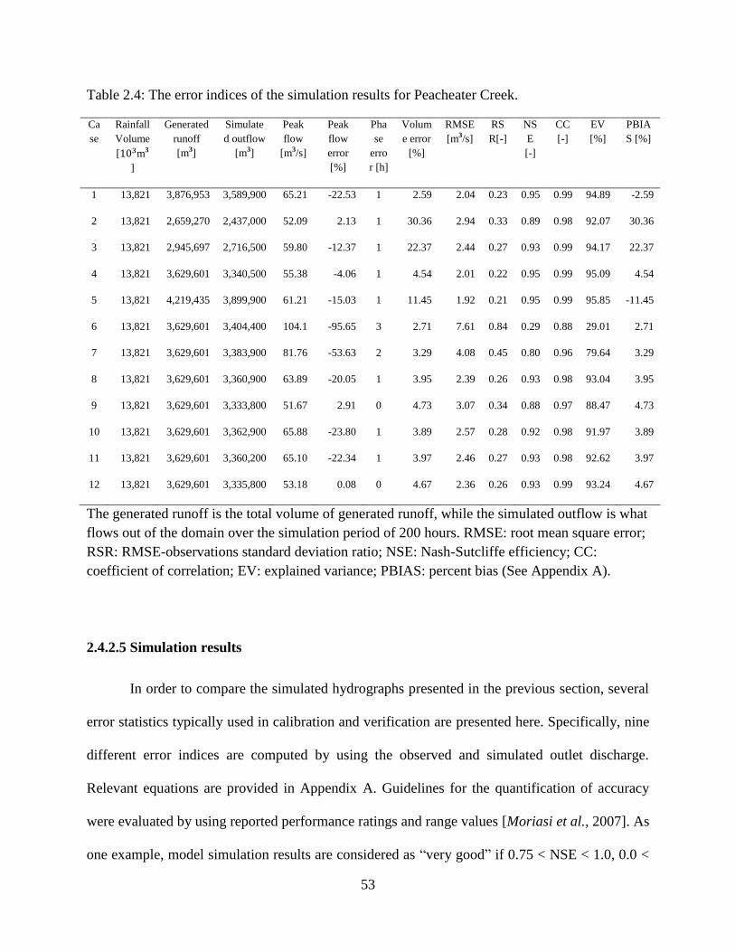
53

Table 2.4: The error indices of the simulation results for Peacheater Creek.

Ca

se

Rainfall

Volume

[ m3

]

Generated

runoff

[m3]

Simulate

d outflow

[m3]

Peak

flow

[m3/s]

Peak

flow

error

[%]

Pha

se

erro

r [h]

Volum

e error

[%]

RMSE

[m3/s]

RS

R[-]

NS

E

[-]

CC

[-]

EV

[%]

PBIA

S [%]

1 13,821 3,876,953 3,589,900 65.21 -22.53 1 2.59 2.04 0.23 0.95 0.99 94.89 -2.59

2 13,821 2,659,270 2,437,000 52.09 2.13 1 30.36 2.94 0.33 0.89 0.98 92.07 30.36

3 13,821 2,945,697 2,716,500 59.80 -12.37 1 22.37 2.44 0.27 0.93 0.99 94.17 22.37

4 13,821 3,629,601 3,340,500 55.38 -4.06 1 4.54 2.01 0.22 0.95 0.99 95.09 4.54

5 13,821 4,219,435 3,899,900 61.21 -15.03 1 11.45 1.92 0.21 0.95 0.99 95.85 -11.45

6 13,821 3,629,601 3,404,400 104.1 -95.65 3 2.71 7.61 0.84 0.29 0.88 29.01 2.71

7 13,821 3,629,601 3,383,900 81.76 -53.63 2 3.29 4.08 0.45 0.80 0.96 79.64 3.29

8 13,821 3,629,601 3,360,900 63.89 -20.05 1 3.95 2.39 0.26 0.93 0.98 93.04 3.95

9 13,821 3,629,601 3,333,800 51.67 2.91 0 4.73 3.07 0.34 0.88 0.97 88.47 4.73

10 13,821 3,629,601 3,362,900 65.88 -23.80 1 3.89 2.57 0.28 0.92 0.98 91.97 3.89

11 13,821 3,629,601 3,360,200 65.10 -22.34 1 3.97 2.46 0.27 0.93 0.98 92.62 3.97

12 13,821 3,629,601 3,335,800 53.18 0.08 0 4.67 2.36 0.26 0.93 0.99 93.24 4.67

The generated runoff is the total volume of generated runoff, while the simulated outflow is what

flows out of the domain over the simulation period of 200 hours. RMSE: root mean square error;

RSR: RMSE-observations standard deviation ratio; NSE: Nash-Sutcliffe efficiency; CC:

coefficient of correlation; EV: explained variance; PBIAS: percent bias (See Appendix A).

2.4.2.5 Simulation results

In order to compare the simulated hydrographs presented in the previous section, several

error statistics typically used in calibration and verification are presented here. Specifically, nine

different error indices are computed by using the observed and simulated outlet discharge.

Relevant equations are provided in Appendix A. Guidelines for the quantification of accuracy

were evaluated by using reported performance ratings and range values [Moriasi et al., 2007]. As

one example, model simulation results are considered as “very good” if 0.75 < NSE < 1.0, 0.0 <

54

RSR < 0.5 and PBIAS < 10 %. According to these criteria, most simulation cases can be

evaluated as “very good”, even though few of them (for the Cases 2, 3, 5 and 6) exhibit small

discrepancies. Cases 4, 9 and 12 show particularly good results in terms of the peak flow error

and volume error. Therefore, Case 4 is used for comparisons throughout the rest of the

manuscript.

Figure 2.18 shows the spatial distribution of the frequency of runoff occurrence as the

fraction of the total simulation time (equal to 200 hours). The pattern of infiltration excess runoff

in the northern region of the basin is due to the particular structure of storm (as inferred from 4

km x 4km radar images) that passed the watershed area. Saturation excess runoff does not exhibit

a particular dependence on the soil type because the infiltration capacity and lateral rates of

moisture redistribution are high. This runoff mechanism, on the other hand, is highly influenced

by topography. Therefore, it frequently occurs near the stream network of the watershed with

large contributing areas and flat slopes of the terrain. The perched return runoff and the

groundwater exfiltration runoff are also mainly generated near the stream network.

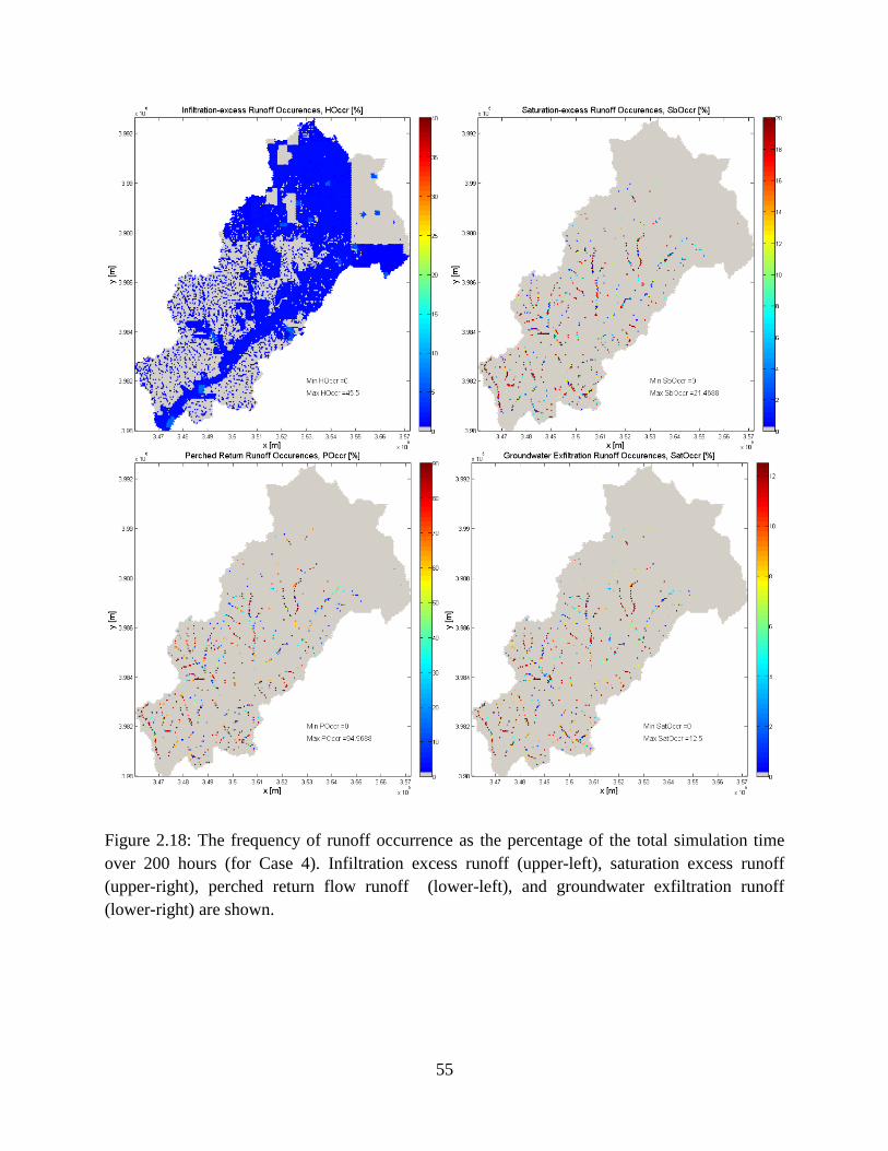
55

Figure 2.18: The frequency of runoff occurrence as the percentage of the total simulation time

over 200 hours (for Case 4). Infiltration excess runoff (upper-left), saturation excess runoff

(upper-right), perched return flow runoff (lower-left), and groundwater exfiltration runoff

(lower-right) are shown.

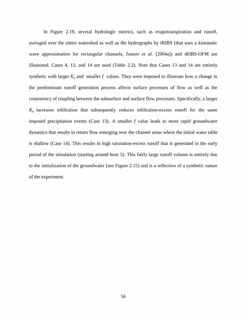
56

In Figure 2.19, several hydrologic metrics, such as evapotranspiration and runoff,

averaged over the entire watershed as well as the hydrographs by tRIBS (that uses a kinematic

wave approximation for rectangular channels, Ivanov et al. [2004a]) and tRIBS-OFM are

illustrated. Cases 4, 13, and 14 are used (Table 2.2). Note that Cases 13 and 14 are entirely

synthetic with larger and smaller f values. They were imposed to illustrate how a change in

the predominant runoff generation process affects surface processes of flow as well as the

consistency of coupling between the subsurface and surface flow processes. Specifically, a larger

increases infiltration that subsequently reduces infiltration-excess runoff for the same

imposed precipitation events (Case 13). A smaller f value leads to more rapid groundwater

dynamics that results in return flow emerging near the channel areas where the initial water table

is shallow (Case 14). This results in high saturation-excess runoff that is generated in the early

period of the simulation (starting around hour 5). This fairly large runoff volume is entirely due

to the initialization of the groundwater (see Figure 2.15) and is a reflection of a synthetic nature

of the experiment.

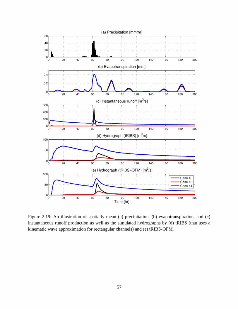
57

Figure 2.19: An illustration of spatially mean (a) precipitation, (b) evapotranspiration, and (c)

instantaneous runoff production as well as the simulated hydrographs by (d) tRIBS (that uses a

kinematic wave approximation for rectangular channels) and (e) tRIBS-OFM.

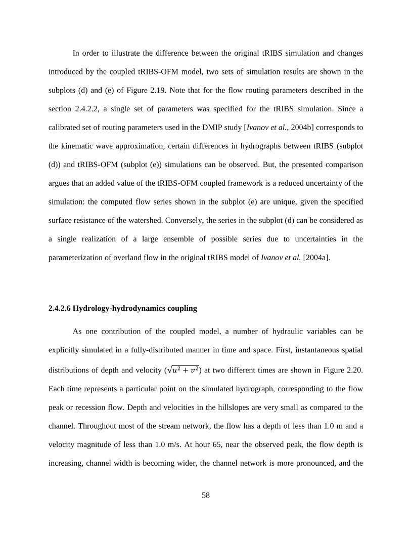
58

In order to illustrate the difference between the original tRIBS simulation and changes

introduced by the coupled tRIBS-OFM model, two sets of simulation results are shown in the

subplots (d) and (e) of Figure 2.19. Note that for the flow routing parameters described in the

section 2.4.2.2, a single set of parameters was specified for the tRIBS simulation. Since a

calibrated set of routing parameters used in the DMIP study [Ivanov et al., 2004b] corresponds to

the kinematic wave approximation, certain differences in hydrographs between tRIBS (subplot

(d)) and tRIBS-OFM (subplot (e)) simulations can be observed. But, the presented comparison

argues that an added value of the tRIBS-OFM coupled framework is a reduced uncertainty of the

simulation: the computed flow series shown in the subplot (e) are unique, given the specified

surface resistance of the watershed. Conversely, the series in the subplot (d) can be considered as

a single realization of a large ensemble of possible series due to uncertainties in the

parameterization of overland flow in the original tRIBS model of Ivanov et al. [2004a].

2.4.2.6 Hydrology-hydrodynamics coupling

As one contribution of the coupled model, a number of hydraulic variables can be

explicitly simulated in a fully-distributed manner in time and space. First, instantaneous spatial

distributions of depth and velocity (√ ) at two different times are shown in Figure 2.20.

Each time represents a particular point on the simulated hydrograph, corresponding to the flow

peak or recession flow. Depth and velocities in the hillslopes are very small as compared to the

channel. Throughout most of the stream network, the flow has a depth of less than 1.0 m and a

velocity magnitude of less than 1.0 m/s. At hour 65, near the observed peak, the flow depth is

increasing, channel width is becoming wider, the channel network is more pronounced, and the

59

flow velocity is higher than at other times. Next, detailed information on the direction and

magnitude of the two-dimensional velocity at hour 65 is shown in Figure 2.21. Most of the

velocity vectors are directed toward the channel from hillslopes, reflecting water accumulation.

On the other hand, only small vectors with the streamwise direction exist within the stream

network because the adopted size of grid cells (50 m resolution) is not sufficiently fine to

represent the channel network. This detailed velocity information is necessary for obtaining other

“derivative” metrics of flow conditions, such as shear stress and vorticity. These variables are

required for investigating the effects of climate and watershed hydrology on soil erosion,

sediment transport, and impacts on fish habitats.

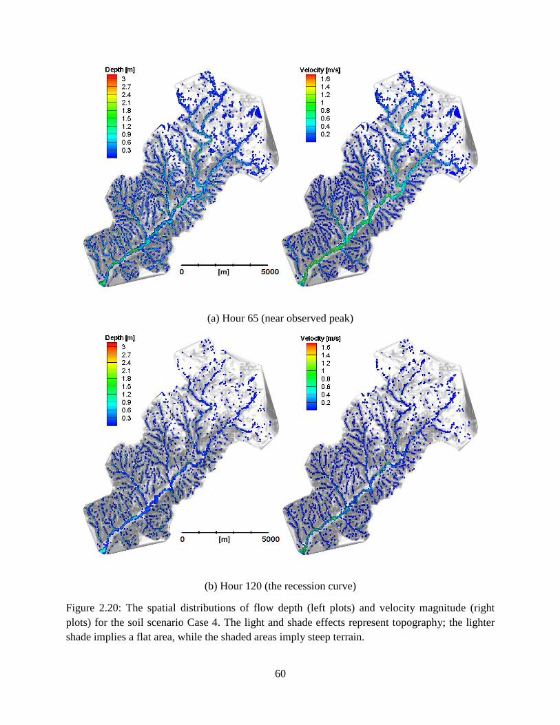
60

(a) Hour 65 (near observed peak)

(b) Hour 120 (the recession curve)

Figure 2.20: The spatial distributions of flow depth (left plots) and velocity magnitude (right

plots) for the soil scenario Case 4. The light and shade effects represent topography; the lighter

shade implies a flat area, while the shaded areas imply steep terrain.

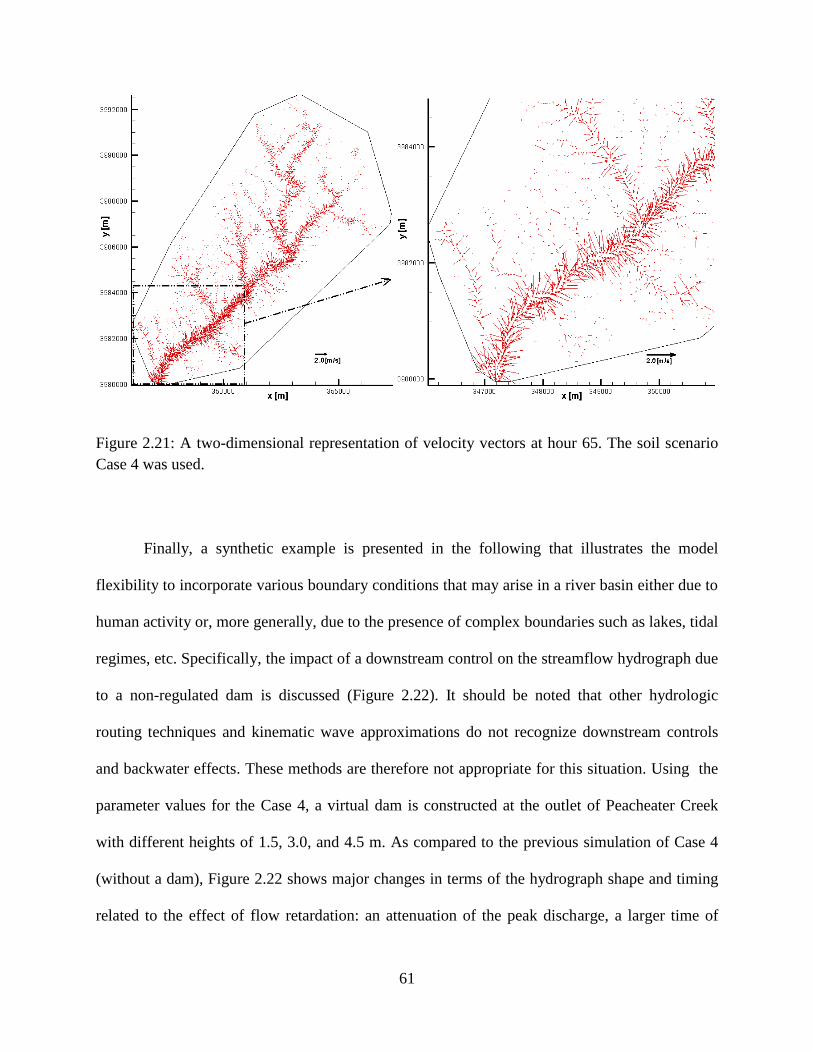
61

Figure 2.21: A two-dimensional representation of velocity vectors at hour 65. The soil scenario

Case 4 was used.

Finally, a synthetic example is presented in the following that illustrates the model

flexibility to incorporate various boundary conditions that may arise in a river basin either due to

human activity or, more generally, due to the presence of complex boundaries such as lakes, tidal

regimes, etc. Specifically, the impact of a downstream control on the streamflow hydrograph due

to a non-regulated dam is discussed (Figure 2.22). It should be noted that other hydrologic

routing techniques and kinematic wave approximations do not recognize downstream controls

and backwater effects. These methods are therefore not appropriate for this situation. Using the

parameter values for the Case 4, a virtual dam is constructed at the outlet of Peacheater Creek

with different heights of 1.5, 3.0, and 4.5 m. As compared to the previous simulation of Case 4

(without a dam), Figure 2.22 shows major changes in terms of the hydrograph shape and timing

related to the effect of flow retardation: an attenuation of the peak discharge, a larger time of

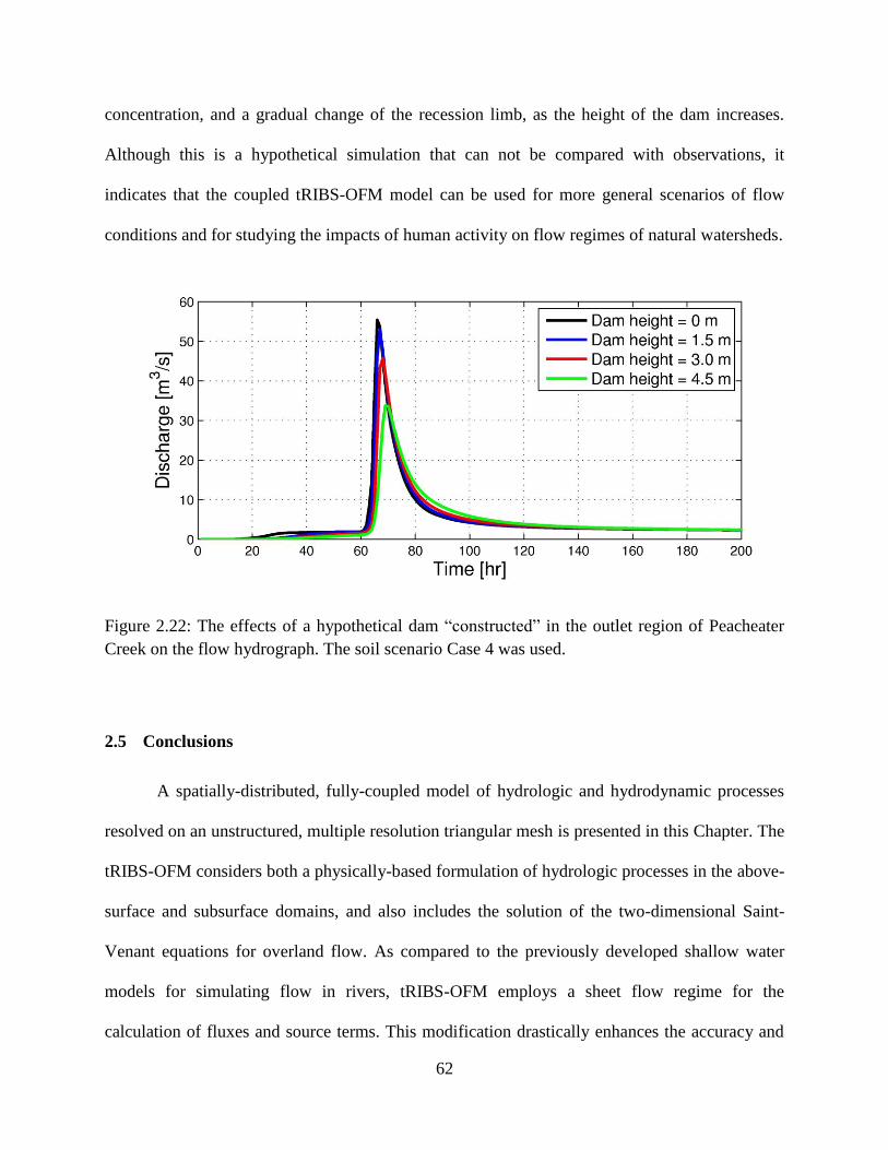
62

concentration, and a gradual change of the recession limb, as the height of the dam increases.

Although this is a hypothetical simulation that can not be compared with observations, it

indicates that the coupled tRIBS-OFM model can be used for more general scenarios of flow

conditions and for studying the impacts of human activity on flow regimes of natural watersheds.

Figure 2.22: The effects of a hypothetical dam “constructed” in the outlet region of Peacheater

Creek on the flow hydrograph. The soil scenario Case 4 was used.

2.5 Conclusions

A spatially-distributed, fully-coupled model of hydrologic and hydrodynamic processes

resolved on an unstructured, multiple resolution triangular mesh is presented in this Chapter. The

tRIBS-OFM considers both a physically-based formulation of hydrologic processes in the above-

surface and subsurface domains, and also includes the solution of the two-dimensional Saint-

Venant equations for overland flow. As compared to the previously developed shallow water

models for simulating flow in rivers, tRIBS-OFM employs a sheet flow regime for the

calculation of fluxes and source terms. This modification drastically enhances the accuracy and

63

consistency of the formulation avoiding the numerical “no-flow phenomenon” in the partially-

submerged cells that occurs in steeply sloped areas with low runoff production rates.

As a consistent outcome of the illustrated applications, the flow model confirms its

sensitivity with respect to surface roughness coefficients and mesh resolution. Specifically, mesh

resolution, especially near the channel and floodplain regions, affects the speed of wave

propagation in the drainage network and thus a coarser mesh has a larger time of concentration.

Insufficient information about roughness characteristics of the domain gives rise to significant

uncertainties associated with flow routing.

The popular kinematic wave assumption may be inappropriate in some parts of the flow

domain. In contrast, the dynamic wave routing method shows more accurate, physically-

consistent results, especially in the areas of confluence of channel and hillslope and the regions

where abrupt transitions of terrain slope occur. Thus, the developed coupled model is an

appropriate tool to use for cases with time-varying flow conditions.

The work of this Chapter expands previous research by adapting a hydrodynamic model

to watershed-scale simulations, which makes it suitable for providing a more coherent and

comprehensive description of runoff phenomena and flow characteristics. The essential strengths

of the coupled model are as follows. 1) The model can solve the overland flow problem in all

situations that cannot be addressed with traditional hydrologic models. These include hydraulic

jumps, backwater conditions, and control structure effects. In particular, tRIBS-OFM is one of a

few existing comprehensive hydrologic-hydrodynamic models that can be used for simulating

flow converging-diverging effects due to microtopographic disturbances and vegetation features

at both micro (cm) and macro (km) scales. 2) The model reduces the uncertainty associated with

64

parameterizations used by traditional hydrologic routing procedures. 3) The model can be used to

obtain detailed information about flow regime characteristics, i.e. the flow depth and velocity. 4)

The model is especially valuable in hydraulic problems related to stream or river domains (e.g.,

flood inundation), where upstream or downstream boundary conditions of a river cannot be

easily specified and need to be computed independently with a hydrologic model. According to

the definition of a drainage watershed, all surface water located within the watershed ultimately

converges to an outlet. Therefore, the coupled model needs only two types of “known” boundary

conditions, i.e., non-transmissible (wall) for all boundaries except for an outlet or transmissible

(open) boundary conditions for an outlet. 5) Finally, if further combined with other geoscience

and engineering models, such as those representing erosion and sediment transport, or a model of

aquatic habitat, the proposed model will be useful for addressing a range of scientific questions,

for example, how meteorological and hydrological signals affect streamflow regimes,

morphological variability, and quality of aquatic habitats.

65

CHAPTER III

Hairsine-Rose erosion equations coupled with hydrological processes and

overland flow at watershed scale: “tRIBS-OFM-HRM”

3.1 Introduction

Soil erosion and excessive sedimentation are among the most important threats to

sustainable agriculture and watershed management worldwide [Oldeman et al., 1991; Bai et al.,

2008]. Erosion leads to significant soil loss [Buringh, 1981; Brown, 1984] and imposes

substantial social costs [Pimentel et al., 1995; Noel, 2001]. Major problems and concerns related

to soil erosion are as follows. (1) Rainfall- and runoff-induced erosion from watersheds and farm

fields produce major non-point source pollutants for many significant environmental resources

[Hogarth et al., 2004b]. (2) River bank erosion and the associated rise of channel bed can lead to

a diminished flow capacity and higher vulnerability to floods. (3) Land degradation caused by

acceleration of agricultural activities, deforestation, and urbanization remove fertile topsoil,

resulting in a decrease of agricultural productivity [Fiener et al., 2008]. (4) Streamflow

characteristics and erosion processes are critical in determining stream physical habitat

properties and can be responsible for undesired ecological impacts on biotic composition [Poff

and Allan, 1995; Bunn and Arthington, 2002; Poff and Zimmerman, 2010].

66

In order to enhance the understanding of the erosion mechanism and investigate how to

reduce social costs, a number of continuing efforts have been undertaken to simulate the erosion

process over the last few decades. Depending on what model is given an emphasis in an overall

approach, studies can be conceptually divided into two classes. First, hydrologically-based

erosion models can be categorized either as empirical or mechanistic. Empirical models are

usually derived by processing data observed at a plot-scale with further application of statistical

or stochastic scaling techniques that extract general characteristics for parsimonious estimation

of soil erosion. These models have been widely used due to their simplicity and reduced

computational cost and data requirements. However, empirical models are limited in their

capabilities: they use lumped parameters that cannot be directly measured in the field and ignore

non-linearities, thus limiting transferability of parameters from one watershed to another.

Conversely, mechanistic or sometimes referred to as “physically based” models originate from

conservation laws with parameters that bear physical meaning. These models enforce mass

conservation and simplified versions of momentum conservation for flow, as well as mass

conservation for sediment that is present in both the flow and stream bed. For a detailed review

of the most commonly used hydrologically-based erosion models, the reader is referred to

Merritt et al. [2003] and Aksoy and Kavvas [2005].

As another type of approach to erosion and sediment transport modeling, hydraulics-

based erosion models focus on accurate solutions of flow mechanisms and coupling sediment

motions to the flow dynamics. These models generally do not consider hydrological processes,

assuming artificial or “known” boundary conditions. They solve various simplified forms of the

Saint-Venant or shallow-water equations combined with advection-dominated sediment transport

equations. Among this type of models that have been recently developed are those reported in

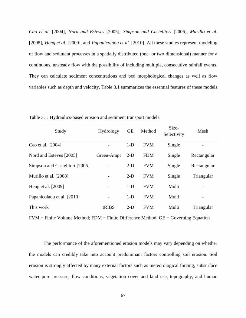
67

Cao et al. [2004], Nord and Esteves [2005], Simpson and Castelltort [2006], Murillo et al.

[2008], Heng et al. [2009], and Papanicolaou et al. [2010]. All these studies represent modeling

of flow and sediment processes in a spatially distributed (one- or two-dimensional) manner for a

continuous, unsteady flow with the possibility of including multiple, consecutive rainfall events.

They can calculate sediment concentrations and bed morphological changes as well as flow

variables such as depth and velocity. Table 3.1 summarizes the essential features of these models.

Table 3.1: Hydraulics-based erosion and sediment transport models.

Study Hydrology GE Method Size-

Selectivity Mesh

Cao et al. [2004] - 1-D FVM Single -

Nord and Esteves [2005] Green-Ampt 2-D FDM Single Rectangular

Simpson and Castelltort [2006] - 2-D FVM Single Rectangular

Murillo et al. [2008] - 2-D FVM Single Triangular

Heng et al. [2009] - 1-D FVM Multi -

Papanicolaou et al. [2010] - 1-D FVM Multi -

This work tRIBS 2-D FVM Multi Triangular

FVM = Finite Volume Method; FDM = Finite Difference Method; GE = Governing Equation

The performance of the aforementioned erosion models may vary depending on whether

the models can credibly take into account predominant factors controlling soil erosion. Soil

erosion is strongly affected by many external factors such as meteorological forcing, subsurface

water pore pressure, flow conditions, vegetation cover and land use, topography, and human

68

activities. It is also influenced by the soil‟s inherent properties such as erodibility, cohesiveness,

and particle size distribution. Among the external factors, meteorological forcing, land use, and

topographic data are typically given as input to an erosion model, and the last two are usually

known at sufficiently high accuracy. Given appropriate meteorological input, the performance of

a model depends mainly on the capability to reproduce the remaining factors: hydrological

dynamics, including subsurface and above-surface phenomena, and hydrodynamic flow motions

caused by complex topography at the watershed scale. Similarly, while soil erodibility and

cohesiveness are considered in many erosion models as parameters, sediment particle size

distribution is not generally included and a single sediment size is used. Overall, among external

and internal factors, hydrological and hydraulic characteristics and particle size distribution are

arguably the three most crucial elements in modeling erosion because of several reasons: (1) the

partition of rainfall into runoff and “losses” (e.g. infiltration) strongly influences the overall

magnitude of sediment erosion; for example, the sensitivity to this partition is very high in semi-

arid areas, where more than 90 percent of precipitation is lost to infiltration [Nearing et al.,

2007]; (2) the two-dimensional spatial variability of hydraulic or sediment state variables due to

precipitation, topography or man-made infrastructures can affect the capability of accurate

prediction of detachment and deposition of sediment; and (3) size differences of bed material

impact the load and spatiotemporal variability of sediment dynamics. From a practical point, it is

particularly valuable to discern fine sediments because many materials that impair water quality

tend to adhere to them.

None of the advanced hydraulics-based erosion studies listed in Table 3.1 consider all of

the crucial factors and thus satisfy the aforementioned needs. Specifically, some of these studies

employ the one-dimensional formulations of governing equations for flow and sediment; only a

69

few studies consider grain-size dependences. Moreover, most of these studies (with the exception

of the study by Nord and Esteves [2005] that uses the Green-Ampt method for estimating runoff-

loss partition) take little account of hydrologic processes at a relevant level of detail. It is

especially of great importance in estimating runoff generation including saturation-excess runoff,

perched and groundwater exfiltration as well as infiltration-excess runoff because it varies

greatly depending on topography, climate, soil type, groundwater table, and initial conditions as

well [Noto et al., 2008]. Therefore, this work represents a first attempt to combine all necessary

processes within a single framework.

Previously developed hydrologic and hydrodynamic models are coupled here with the

Hairsine-Rose (H-R) formulation [Hairsine and Rose, 1991; 1992; Sander et al., 2007a] to

describe soil erosion and sediment transport. The H-R model can account for size-selective

sediment transport based on particle size distribution. The formulation differentiates composition

of the bed into original and deposited soil layers, recognizing whether material has an “intact” or

a “loose” condition. Formulations of the governing equations and a description of the numerical

model are provided in Sections 3.2 and 3.3. Model verification is subsequently carried out, in

which simulation results are compared with analytical solutions and empirical data. Two

benchmark laboratory cases dealing with rainfall-induced erosion and overland flow-induced

erosion are used. The numerical model is further applied at catchment scale to the Lucky Hills

watershed located in southeastern Arizona, U.S.A. Before calibration, we performed two

sensitivity tests to a grid resolution and the number of particle size. Model confirmation is then

carried out for the outlet using observed data for ten rainfall events with parameter values

obtained through calibration for a single rainfall event. An analysis of spatially distributed size-

dependent dynamics concludes this manuscript.

70

3.2 Governing equations

The present numerical model is comprised of three primary components: hydrology

(tRIBS), flow dynamics (OFM), and erosion and sediment transport (H-R model). Governing

equations or methods for the description of hydrologic processes considered in tRIBS are

summarized in Table 2.1; for more detailed information, the reader is referred to Ivanov et al.

[2004a]. Furthermore, the overland flow model was formerly developed by Bradford and

Katopodes [1999] for simulating turbid underflows and was later extended to an unstructured

triangular mesh [Begnudelli and Sanders, 2006]. It has been successfully used for a wide range

of hydrodynamic applications of surface irrigation [Bradford and Katopodes, 2001], dam break-

[Begnudelli and Sanders, 2007; Begnudelli et al., 2008] or urban- [Sanders et al., 2008] flooding

phenomenon, and efficiency enhancement through a Local Time Stepping scheme [Sanders,

2008]. Most details of unstructured mesh formulation such as neighboring mapping functions are

followed by the approach of Begnudelli and Sanders [2006].

For the purpose of attaining a numerical solution in the erosion and sediment transport

problem, the two-dimensional (2-D) Saint-Venant equations coupled with a formulation of

sediment mass conservation and bed morphology evolution are used. The 2-D Saint-Venant

equations are based on the assumption of hydrostatic pressure distribution in the vertical, so they

are appropriate for vertically-mixed water bodies. These equations, based on a vertical

coordinate system, in conservative form are as follows

√

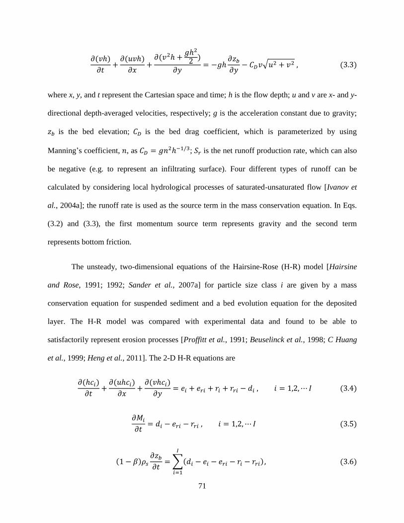
71

√

where x, y, and t represent the Cartesian space and time; h is the flow depth; u and v are x- and y-

directional depth-averaged velocities, respectively; g is the acceleration constant due to gravity;

is the bed elevation; is the bed drag coefficient, which is parameterized by using

Manning‟s coefficient, , as ; is the net runoff production rate, which can also

be negative (e.g. to represent an infiltrating surface). Four different types of runoff can be

calculated by considering local hydrological processes of saturated-unsaturated flow [Ivanov et

al., 2004a]; the runoff rate is used as the source term in the mass conservation equation. In Eqs.

(3.2) and (3.3), the first momentum source term represents gravity and the second term

represents bottom friction.

The unsteady, two-dimensional equations of the Hairsine-Rose (H-R) model [Hairsine

and Rose, 1991; 1992; Sander et al., 2007a] for particle size class i are given by a mass

conservation equation for suspended sediment and a bed evolution equation for the deposited

layer. The H-R model was compared with experimental data and found to be able to

satisfactorily represent erosion processes [Proffitt et al., 1991; Beuselinck et al., 1998; C Huang

et al., 1999; Heng et al., 2011]. The 2-D H-R equations are

∑

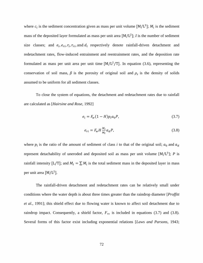
72

where is the sediment concentration given as mass per unit volume ; is the sediment

mass of the deposited layer formulated as mass per unit area ; I is the number of sediment

size classes; and respectively denote rainfall-driven detachment and

redetachment rates, flow-induced entrainment and reentrainment rates, and the deposition rate

formulated as mass per unit area per unit time . In equation (3.6), representing the

conservation of soil mass, is the porosity of original soil and is the density of solids

assumed to be uniform for all sediment classes.

To close the system of equations, the detachment and redetachment rates due to rainfall

are calculated as [Hairsine and Rose, 1992]

(3.7)

(3.8)

where is the ratio of the amount of sediment of class i to that of the original soil; and

represent detachability of uneroded and deposited soil as mass per unit volume [ ]; P is

rainfall intensity ; and ∑ is the total sediment mass in the deposited layer in mass

per unit area .

The rainfall-driven detachment and redetachment rates can be relatively small under

conditions where the water depth is about three times greater than the raindrop diameter [Proffitt

et al., 1991]; this shield effect due to flowing water is known to affect soil detachment due to

raindrop impact. Consequently, a shield factor, Fw, is included in equations (3.7) and (3.8).

Several forms of this factor exist including exponential relations [Laws and Parsons, 1943;

73

Mutchler and McGregor, 1983] or a power law [Proffitt et al., 1991]. Using the power law

relation by Proffitt et al. [1991], the shield factor is formulated as

(3.9)

where a threshold of is used, where is the mean raindrop size. An exponent b

varies depending on the type of soil and can be obtained with a best fit using experimental data,

e.g., for clay, b=0.66 [Proffitt et al., 1991], and for loam, b=1.13 [Mutchler and McGregor,

1983].

The proportion of shielding of the deposited layer, H, is calculated as

, where

is a calibrated parameter denoting the mass of deposited sediment

needed to completely sheild the original soil, given as mass per unit area . Note that the

shield factor Fw is included in this relation using an analogy that the shield mass is expected to

vary linearly with the rainfall redetachability, i.e., is a constant. [Heng et al., 2011].

The entrainment and reentrainment rates due to overland flow are evaluated as follows

[Hairsine and Rose, 1992]

(3.10)

(3.11)

where is the stream power [Bagnold, 1966] in units of , computed as

√ , where ; is the critical stream power, below which

soil entrainment or reentrainment do not occur; F is the effective fraction of excess stream power

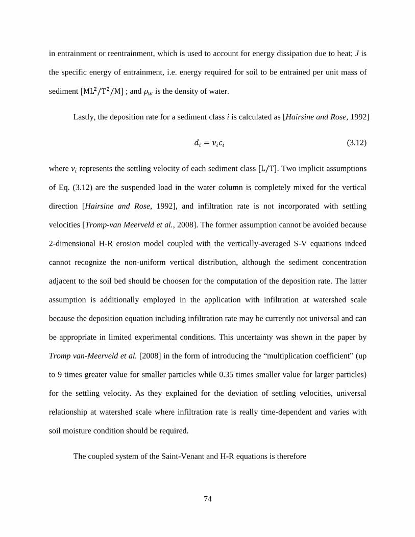
74

in entrainment or reentrainment, which is used to account for energy dissipation due to heat; J is

the specific energy of entrainment, i.e. energy required for soil to be entrained per unit mass of

sediment ; and is the density of water.

Lastly, the deposition rate for a sediment class i is calculated as [Hairsine and Rose, 1992]

(3.12)

where represents the settling velocity of each sediment class . Two implicit assumptions

of Eq. (3.12) are the suspended load in the water column is completely mixed for the vertical

direction [Hairsine and Rose, 1992], and infiltration rate is not incorporated with settling

velocities [Tromp-van Meerveld et al., 2008]. The former assumption cannot be avoided because

2-dimensional H-R erosion model coupled with the vertically-averaged S-V equations indeed

cannot recognize the non-uniform vertical distribution, although the sediment concentration

adjacent to the soil bed should be choosen for the computation of the deposition rate. The latter

assumption is additionally employed in the application with infiltration at watershed scale

because the deposition equation including infiltration rate may be currently not universal and can

be appropriate in limited experimental conditions. This uncertainty was shown in the paper by

Tromp van-Meerveld et al. [2008] in the form of introducing the “multiplication coefficient” (up

to 9 times greater value for smaller particles while 0.35 times smaller value for larger particles)

for the settling velocity. As they explained for the deviation of settling velocities, universal

relationship at watershed scale where infiltration rate is really time-dependent and varies with

soil moisture condition should be required.

The coupled system of the Saint-Venant and H-R equations is therefore

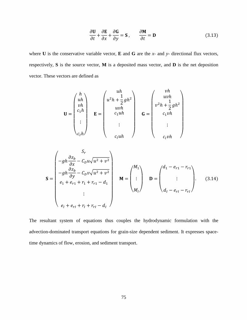
75

where U is the conservative variable vector, E and G are the x- and y- directional flux vectors,

respectively, S is the source vector, M is a deposited mass vector, and D is the net deposition

vector. These vectors are defined as

(

)

(

)

(

)

(

√

√

)

(

)

(

)

The resultant system of equations thus couples the hydrodynamic formulation with the

advection-dominated transport equations for grain-size dependent sediment. It expresses space-

time dynamics of flow, erosion, and sediment transport.

76

3.3 Numerical model

The hydrologic model operates in a continuous fashion, simulating conditions of both

storm and interstorm periods, propagating these conditions to both subsurface states and flow

regimes. Consequently, hydrologic applications inevitably encounter flow conditions associated

with low precipitation and runoff rates that result in many partially-submerged mesh cells [Kim

et al., 2012b]. Tracking and handling wet and dry fronts occurring in these cells has traditionally

been of great interest and generally treated by using the information of neighboring wet cells

[Titov and Synolakis, 1995; Bradford and Sanders, 2002; Xia et al., 2010] and by modifying the

bed level difference [Brufau and Garcia-Navarro, 2003; Brufau et al., 2004]. However, such

approaches were developed based on hydraulic applications such as flood propagation and wave

runup, and were not targeted in hydrologic, watershed-scale applications that have steeply sloped

cells with dry conditions encountered throughout the simulation. As a result, these cells can

cause a numerical artifact so called “no-flow phenomenon” that hampers an accurate calculation

of the flux, bottom slope, and friction slope terms [Kim et al., 2012b]. This phenomenon refers to

a situation when runoff is stored within a cell without the possibility to flow out. So, the

generated runoff fills up the cell until it becomes inundated, i.e. “wet” cells. This numerical

problem is very critical in domains characterized by high bed slopes and low flow conditions

(e.g., hillslope areas of the watershed). Previously developed shallow water models for

simulating flow in rivers have not addressed this numerical problem. The tRIBS-OFM model

resolved it by using a representation of the sheet flow regime; this modification significantly

enhanced the accuracy of calculation of fluxes and source terms. A more detailed description of

the differences between the hydrologic and hydrodynamic approaches in dealing with wet/dry

situations is provided in the Chapter 2.2.3.

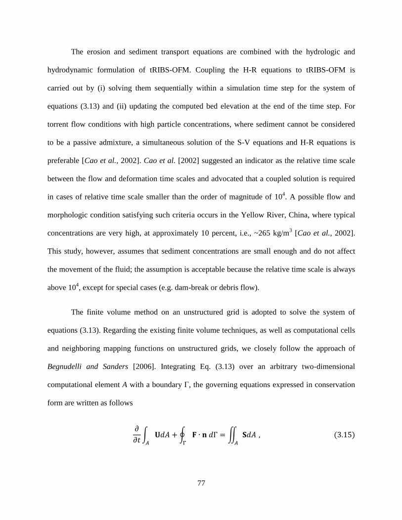
77

The erosion and sediment transport equations are combined with the hydrologic and

hydrodynamic formulation of tRIBS-OFM. Coupling the H-R equations to tRIBS-OFM is

carried out by (i) solving them sequentially within a simulation time step for the system of

equations (3.13) and (ii) updating the computed bed elevation at the end of the time step. For

torrent flow conditions with high particle concentrations, where sediment cannot be considered

to be a passive admixture, a simultaneous solution of the S-V equations and H-R equations is

preferable [Cao et al., 2002]. Cao et al. [2002] suggested an indicator as the relative time scale

between the flow and deformation time scales and advocated that a coupled solution is required

in cases of relative time scale smaller than the order of magnitude of 104. A possible flow and

morphologic condition satisfying such criteria occurs in the Yellow River, China, where typical

concentrations are very high, at approximately 10 percent, i.e., ~265 kg/m3 [Cao et al., 2002].

This study, however, assumes that sediment concentrations are small enough and do not affect

the movement of the fluid; the assumption is acceptable because the relative time scale is always

above 104, except for special cases (e.g. dam-break or debris flow).

The finite volume method on an unstructured grid is adopted to solve the system of

equations (3.13). Regarding the existing finite volume techniques, as well as computational cells

and neighboring mapping functions on unstructured grids, we closely follow the approach of

Begnudelli and Sanders [2006]. Integrating Eq. (3.13) over an arbitrary two-dimensional

computational element A with a boundary Γ, the governing equations expressed in conservation

form are written as follows

∫ ∮ ∬

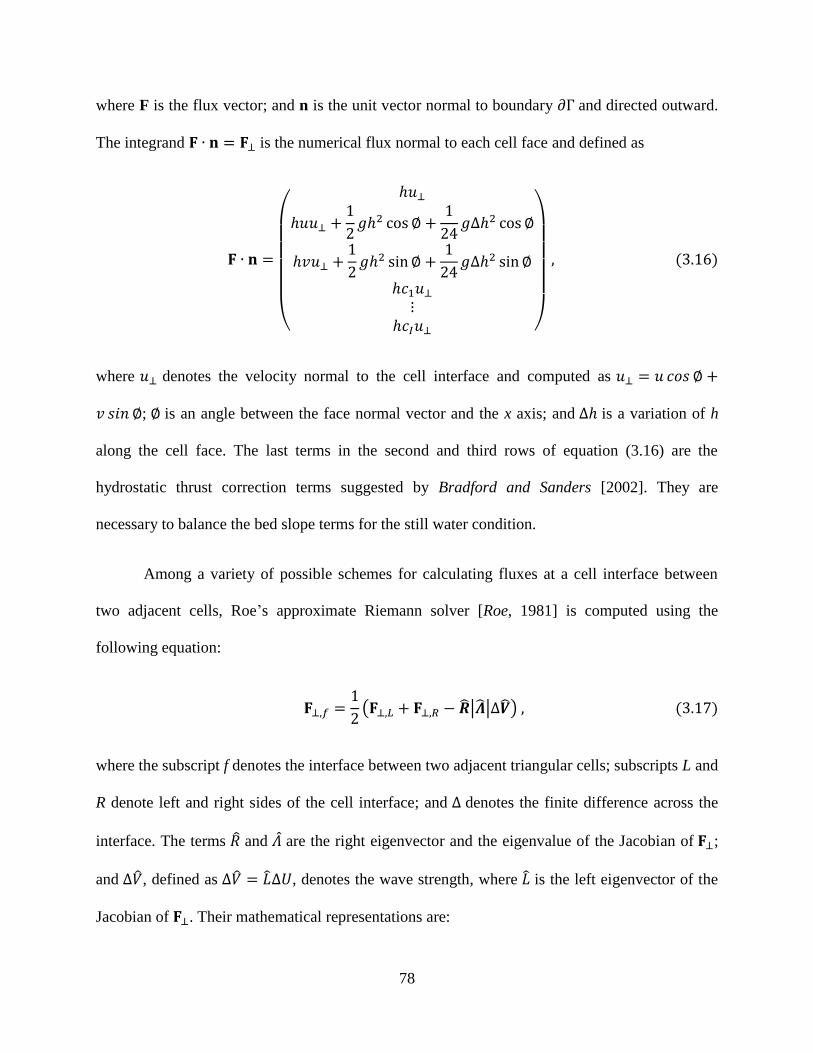
78

where F is the flux vector; and n is the unit vector normal to boundary and directed outward.

The integrand is the numerical flux normal to each cell face and defined as

(

)

where denotes the velocity normal to the cell interface and computed as

; is an angle between the face normal vector and the x axis; and is a variation of h

along the cell face. The last terms in the second and third rows of equation (3.16) are the

hydrostatic thrust correction terms suggested by Bradford and Sanders [2002]. They are

necessary to balance the bed slope terms for the still water condition.

Among a variety of possible schemes for calculating fluxes at a cell interface between

two adjacent cells, Roe‟s approximate Riemann solver [Roe, 1981] is computed using the

following equation:

( | | )

where the subscript f denotes the interface between two adjacent triangular cells; subscripts L and

R denote left and right sides of the cell interface; and denotes the finite difference across the

interface. The terms and are the right eigenvector and the eigenvalue of the Jacobian of ;

and , defined as , denotes the wave strength, where is the left eigenvector of the

Jacobian of . Their mathematical representations are:

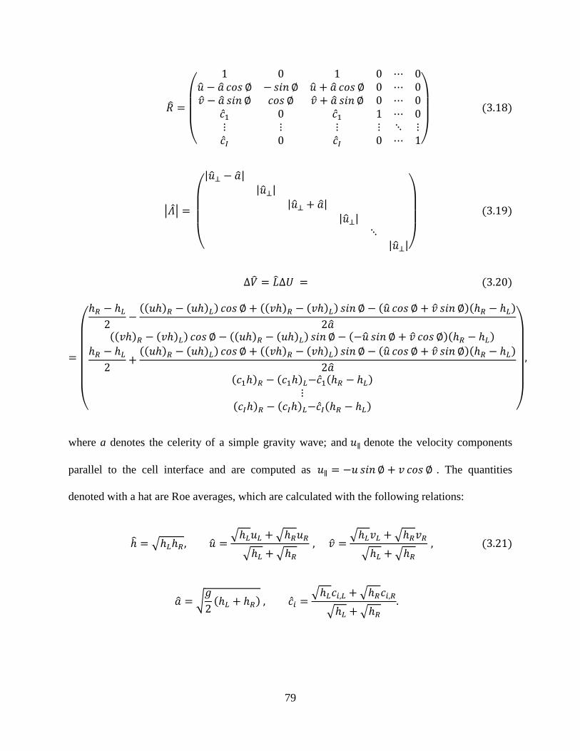
79

(

)

| |

(

| |

| |

| |

| |

| |)

(

)

where a denotes the celerity of a simple gravity wave; and denote the velocity components

parallel to the cell interface and are computed as . The quantities

denoted with a hat are Roe averages, which are calculated with the following relations:

√ √ √

√ √

√ √

√ √

√

√ √

√ √

80

Since Roe‟s method does not calculate the correct flux for critical flow, a local depression wave

is introduced at critical flow locations by replacing the first and third eigenvalues with the

following equation [C Hirsch, 1990]:

| |

where . This relation is used when - | | and the other

eigenvalues, | |, remain unmodified.

Under the assumption that all source terms in the flow and erosion equations are constant

within a cell triangle, they are calculated as

∬

In the computation of the bottom slope, the gradient of is obtained by applying Green‟s

theorem to transform the area integral to the line integral. Thus, the integration of along the

cell boundaries gives

where the subscripts 0, 1 and 2 are three counter-clockwise vertices of a cell triangle. All

variables used for computations of source terms are evaluated at the cell center.

Finally, Eq. (3.13) and Eq. (3.6) are solved by using the following update equation

[

∑

]

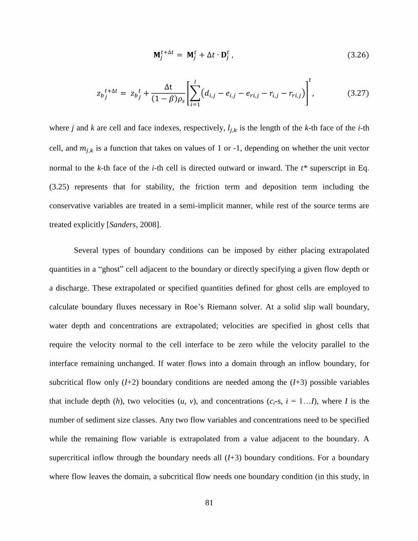
81

[∑( )

]

where j and k are cell and face indexes, respectively, is the length of the k-th face of the i-th

cell, and is a function that takes on values of 1 or -1, depending on whether the unit vector

normal to the k-th face of the i-th cell is directed outward or inward. The t* superscript in Eq.

(3.25) represents that for stability, the friction term and deposition term including the

conservative variables are treated in a semi-implicit manner, while rest of the source terms are

treated explicitly [Sanders, 2008].

Several types of boundary conditions can be imposed by either placing extrapolated

quantities in a “ghost” cell adjacent to the boundary or directly specifying a given flow depth or

a discharge. These extrapolated or specified quantities defined for ghost cells are employed to

calculate boundary fluxes necessary in Roe‟s Riemann solver. At a solid slip wall boundary,

water depth and concentrations are extrapolated; velocities are specified in ghost cells that

require the velocity normal to the cell interface to be zero while the velocity parallel to the

interface remaining unchanged. If water flows into a domain through an inflow boundary, for

subcritical flow only (I+2) boundary conditions are needed among the (I+3) possible variables

that include depth (h), two velocities (u, v), and concentrations (ci-s, i = 1…I), where I is the

number of sediment size classes. Any two flow variables and concentrations need to be specified

while the remaining flow variable is extrapolated from a value adjacent to the boundary. A

supercritical inflow through the boundary needs all (I+3) boundary conditions. For a boundary

where flow leaves the domain, a subcritical flow needs one boundary condition (in this study, in

82

the form of free outfall or zero-depth gradient boundary condition), while no boundary condition

is needed for a supercritical flow.

The proposed model is based on an explicit time integration scheme and thus a stability

restriction, the Courant-Friedrichs-Lewy (CFL) condition, must be satisfied in each cell. For a

triangular mesh, the time step in the model is defined as [Begnudelli and Sanders, 2006]:

, |

|

-

where Cr is the Courant number, is the number of cells, and

is the wave speed normal to

the k-th face of the j-th cell. Furthermore, the restriction on the time step presented by Heng et al.

[2009] is also considered. Specifically, negative concentrations should not be generated and an

approximate estimate of the corresponding time step is

( )

This relation usually limits the time step because it yields estimates that are smaller than those

obtained with the CFL criteria.

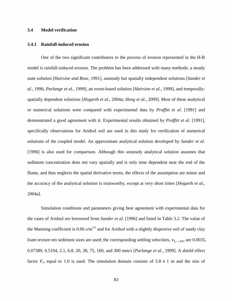
83

3.4 Model verification

3.4.1 Rainfall-induced erosion

One of the two significant contributors to the process of erosion represented in the H-R

model is rainfall-induced erosion. The problem has been addressed with many methods: a steady

state solution [Hairsine and Rose, 1991], unsteady but spatially independent solutions [Sander et

al., 1996; Parlange et al., 1999], an event-based solution [Hairsine et al., 1999], and temporally-

spatially dependent solutions [Hogarth et al., 2004a; Heng et al., 2009]. Most of these analytical

or numerical solutions were compared with experimental data by Proffitt et al. [1991] and

demonstrated a good agreement with it. Experimental results obtained by Proffitt et al. [1991],

specifically observations for Aridsol soil are used in this study for verification of numerical

solutions of the coupled model. An approximate analytical solution developed by Sander et al.

[1996] is also used for comparison. Although this unsteady analytical solution assumes that

sediment concentration does not vary spatially and is only time dependent near the end of the

flume, and thus neglects the spatial derivative terms, the effects of the assumption are minor and

the accuracy of the analytical solution is trustworthy, except at very short times [Hogarth et al.,

2004a].

Simulation conditions and parameters giving best agreement with experimental data for

the cases of Aridsol are borrowed from Sander et al. [1996] and listed in Table 3.2. The value of

the Manning coefficient is 0.06 s/m1/3

and for Aridsol with a slightly dispersive soil of sandy clay

loam texture ten sediment sizes are used; the corresponding settling velocities, , are 0.0035,

0.07389, 0.5194, 2.1, 6.8, 20, 38, 75, 160, and 300 mm/s [Parlange et al., 1999]. A shield effect

factor Fw equal to 1.0 is used. The simulation domain consists of 5.8 1 m and the size of

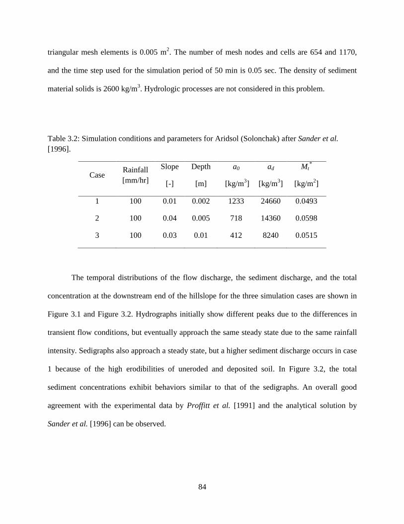
84

triangular mesh elements is 0.005 m2. The number of mesh nodes and cells are 654 and 1170,

and the time step used for the simulation period of 50 min is 0.05 sec. The density of sediment

material solids is 2600 kg/m3. Hydrologic processes are not considered in this problem.

Table 3.2: Simulation conditions and parameters for Aridsol (Solonchak) after Sander et al.

[1996].

Case Rainfall

[mm/hr]

Slope

[-]

Depth

[m]

a0

[kg/m3]

ad

[kg/m3]

Mt*

[kg/m2]

1 100 0.01 0.002 1233 24660 0.0493

2 100 0.04 0.005 718 14360 0.0598

3 100 0.03 0.01 412 8240 0.0515

The temporal distributions of the flow discharge, the sediment discharge, and the total

concentration at the downstream end of the hillslope for the three simulation cases are shown in

Figure 3.1 and Figure 3.2. Hydrographs initially show different peaks due to the differences in

transient flow conditions, but eventually approach the same steady state due to the same rainfall

intensity. Sedigraphs also approach a steady state, but a higher sediment discharge occurs in case

1 because of the high erodibilities of uneroded and deposited soil. In Figure 3.2, the total

sediment concentrations exhibit behaviors similar to that of the sedigraphs. An overall good

agreement with the experimental data by Proffitt et al. [1991] and the analytical solution by

Sander et al. [1996] can be observed.

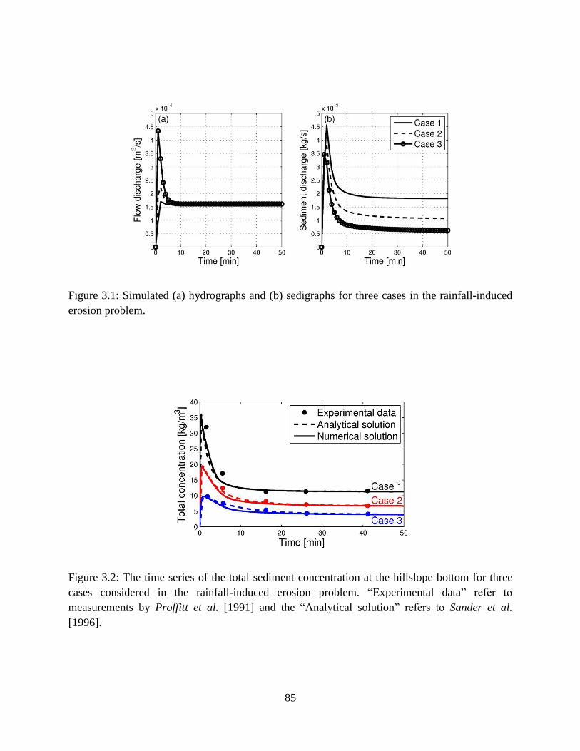
85

Figure 3.1: Simulated (a) hydrographs and (b) sedigraphs for three cases in the rainfall-induced

erosion problem.

Figure 3.2: The time series of the total sediment concentration at the hillslope bottom for three

cases considered in the rainfall-induced erosion problem. “Experimental data” refer to

measurements by Proffitt et al. [1991] and the “Analytical solution” refers to Sander et al.

[1996].

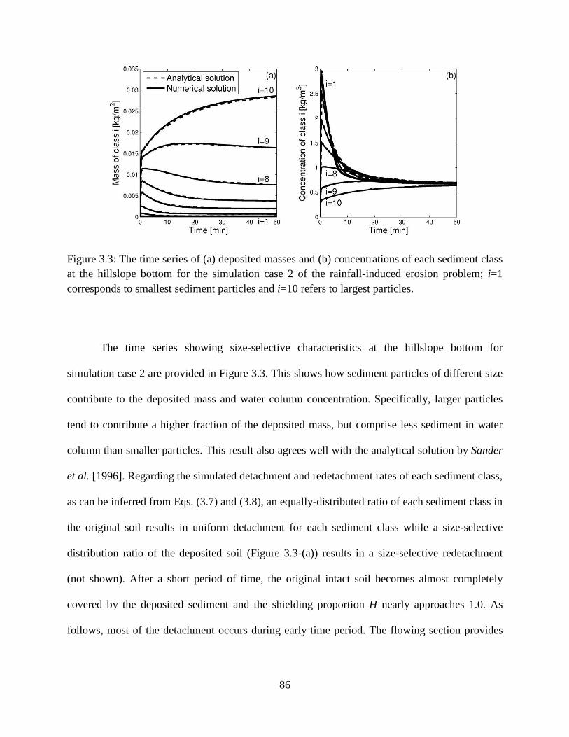
86

Figure 3.3: The time series of (a) deposited masses and (b) concentrations of each sediment class

at the hillslope bottom for the simulation case 2 of the rainfall-induced erosion problem; i=1

corresponds to smallest sediment particles and i=10 refers to largest particles.

The time series showing size-selective characteristics at the hillslope bottom for

simulation case 2 are provided in Figure 3.3. This shows how sediment particles of different size

contribute to the deposited mass and water column concentration. Specifically, larger particles

tend to contribute a higher fraction of the deposited mass, but comprise less sediment in water

column than smaller particles. This result also agrees well with the analytical solution by Sander

et al. [1996]. Regarding the simulated detachment and redetachment rates of each sediment class,

as can be inferred from Eqs. (3.7) and (3.8), an equally-distributed ratio of each sediment class in

the original soil results in uniform detachment for each sediment class while a size-selective

distribution ratio of the deposited soil (Figure 3.3-(a)) results in a size-selective redetachment

(not shown). After a short period of time, the original intact soil becomes almost completely

covered by the deposited sediment and the shielding proportion H nearly approaches 1.0. As

follows, most of the detachment occurs during early time period. The flowing section provides

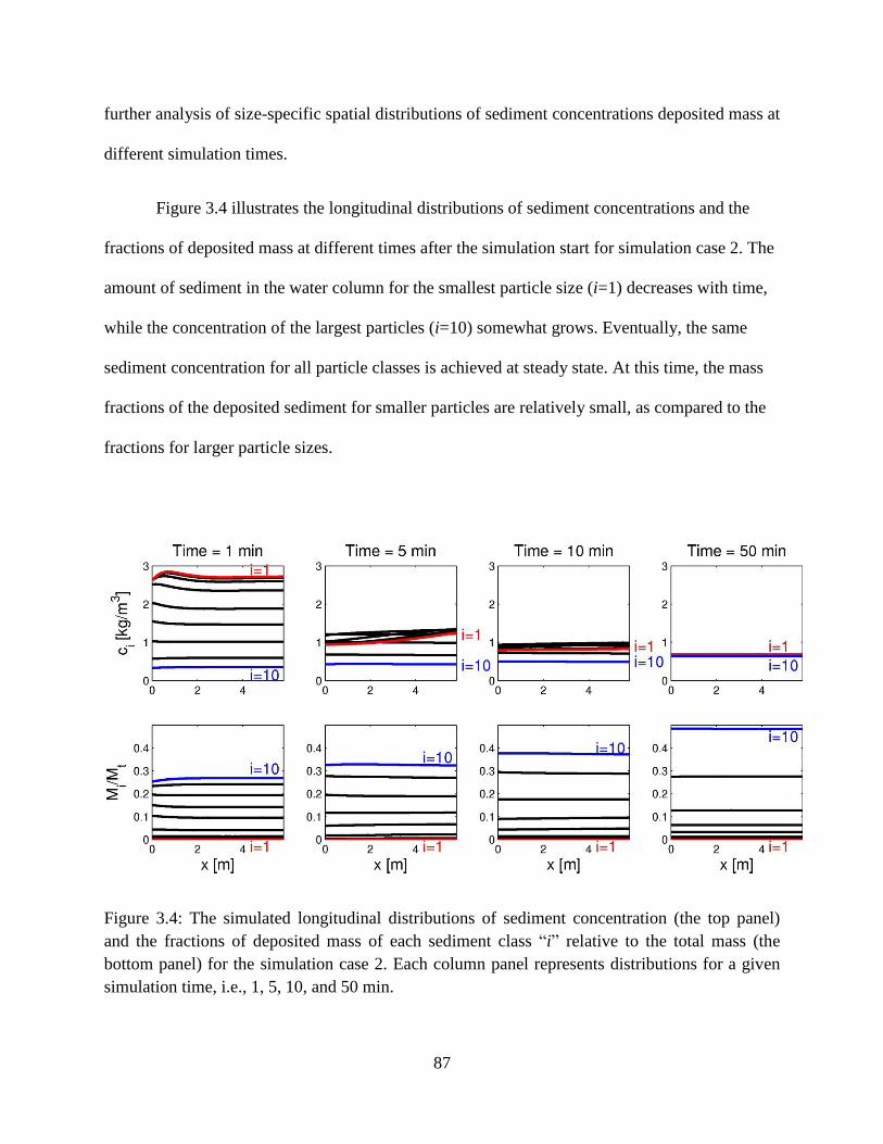
87

further analysis of size-specific spatial distributions of sediment concentrations deposited mass at

different simulation times.

Figure 3.4 illustrates the longitudinal distributions of sediment concentrations and the

fractions of deposited mass at different times after the simulation start for simulation case 2. The

amount of sediment in the water column for the smallest particle size (i=1) decreases with time,

while the concentration of the largest particles (i=10) somewhat grows. Eventually, the same

sediment concentration for all particle classes is achieved at steady state. At this time, the mass

fractions of the deposited sediment for smaller particles are relatively small, as compared to the

fractions for larger particle sizes.

Figure 3.4: The simulated longitudinal distributions of sediment concentration (the top panel)

and the fractions of deposited mass of each sediment class “i” relative to the total mass (the

bottom panel) for the simulation case 2. Each column panel represents distributions for a given

simulation time, i.e., 1, 5, 10, and 50 min.

88

3.4.2 Overland flow-induced erosion

In order to evaluate and verify the overland flow-induced erosion component of the H-R

model, a sediment-laden overland flow problem [Beuselinck et al., 1999; Sander et al., 2002;

Heng et al., 2009] is presented. An overland flow rate of 0.00125 m3/s is imposed at the hillslope

upstream boundary; Concentrations of 10 kg/m3 are specified for all sediment classes, which

results in a net deposition of sediment over the domain. The parameter values are specified as

follows: the Manning coefficient is 0.01 s/m1/3

, the critical stream power is 0.18639 W/m2, the

effective fraction of excess stream power is 0.01, the slope of domain is 0.02, the density of

sediment is 2600 kg/m3, and the settling velocities, , are 0.00043, 0.0037, 0.02, 0.083, 0.23,

0.46, 0.74, 1.1, 1.7, and 3.2 mm/s, respectively. The simulation domain has the dimensions of 10

1 m and the size of mesh elements is 0.005 m2. The number of mesh nodes and triangular cells

are 1116 and 2010, respectively. The time step used during the simulation period of 6 min is

0.005 sec. Hydrologic components are not considered in this problem.

The flow imposed as a boundary condition reaches the outlet and the system achieves

steady-state nearly immediately (not shown). The total sediment yield at the outlet contains

primarily finer particles as compared to coarser sediments. This is consistent with a theoretical

understanding of overland flow erosion: lighter soil particles are more easily moved away from

their sites of origin, as compared to slowly moving heavier particles. The spatial distributions of

concentrations and mass fractions of each sediment class at steady-state are compared with an

analytical solution of Sander et al. [2002] in Figure 3.5. Although small differences are present

in the simulated concentrations of larger particles near the upstream end, an overall good

agreement of the simulation results with the analytical solution can be observed. This might be

because of kinematic vs. dynamic computation effect and boundary condition effect. Since only

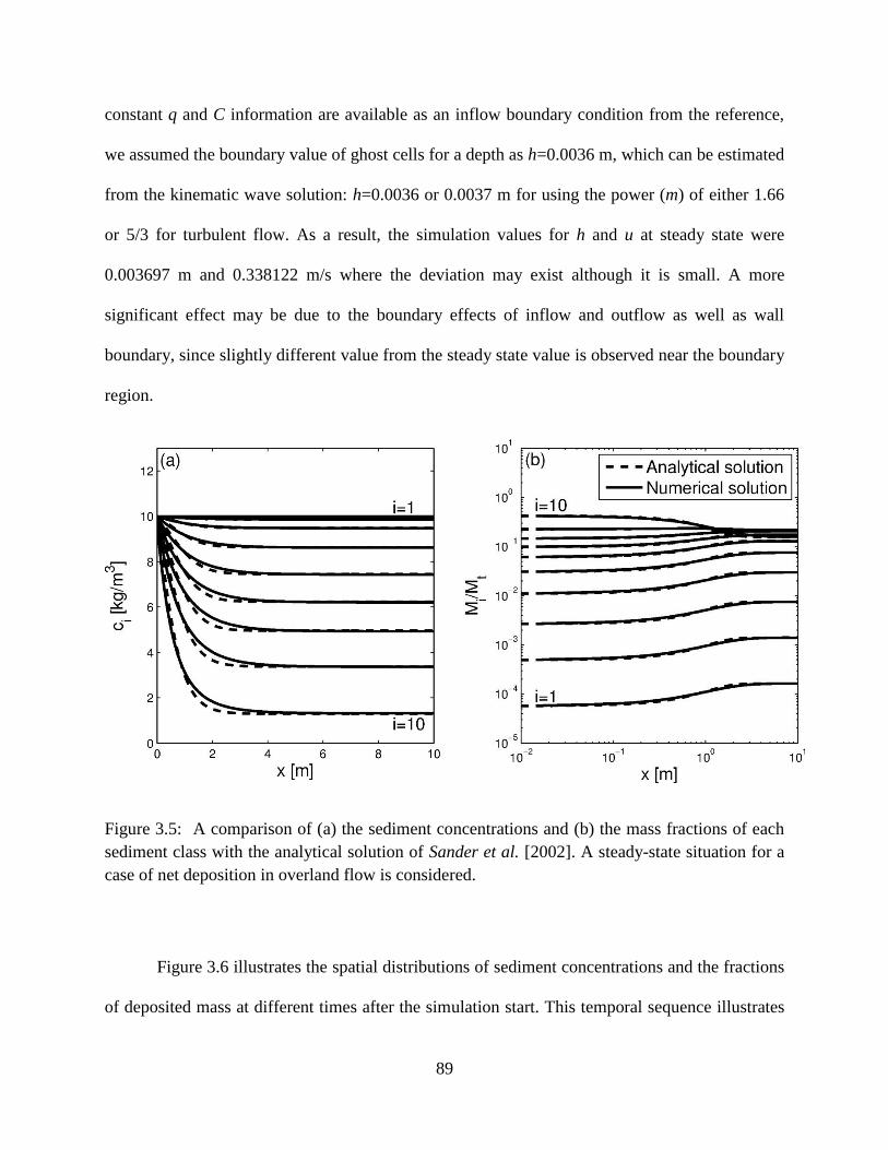
89

constant q and C information are available as an inflow boundary condition from the reference,

we assumed the boundary value of ghost cells for a depth as h=0.0036 m, which can be estimated

from the kinematic wave solution: h=0.0036 or 0.0037 m for using the power (m) of either 1.66

or 5/3 for turbulent flow. As a result, the simulation values for h and u at steady state were

0.003697 m and 0.338122 m/s where the deviation may exist although it is small. A more

significant effect may be due to the boundary effects of inflow and outflow as well as wall

boundary, since slightly different value from the steady state value is observed near the boundary

region.

Figure 3.5: A comparison of (a) the sediment concentrations and (b) the mass fractions of each

sediment class with the analytical solution of Sander et al. [2002]. A steady-state situation for a

case of net deposition in overland flow is considered.

Figure 3.6 illustrates the spatial distributions of sediment concentrations and the fractions

of deposited mass at different times after the simulation start. This temporal sequence illustrates

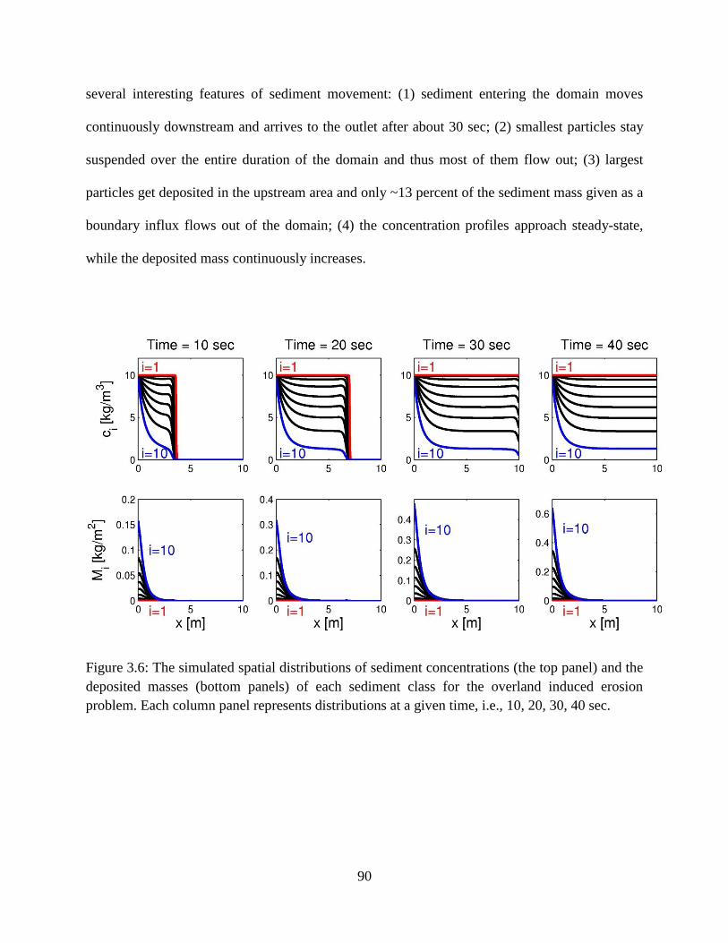
90

several interesting features of sediment movement: (1) sediment entering the domain moves

continuously downstream and arrives to the outlet after about 30 sec; (2) smallest particles stay

suspended over the entire duration of the domain and thus most of them flow out; (3) largest

particles get deposited in the upstream area and only ~13 percent of the sediment mass given as a

boundary influx flows out of the domain; (4) the concentration profiles approach steady-state,

while the deposited mass continuously increases.

Figure 3.6: The simulated spatial distributions of sediment concentrations (the top panel) and the

deposited masses (bottom panels) of each sediment class for the overland induced erosion

problem. Each column panel represents distributions at a given time, i.e., 10, 20, 30, 40 sec.

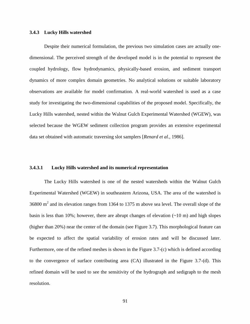
91

3.4.3 Lucky Hills watershed

Despite their numerical formulation, the previous two simulation cases are actually one-

dimensional. The perceived strength of the developed model is in the potential to represent the

coupled hydrology, flow hydrodynamics, physically-based erosion, and sediment transport

dynamics of more complex domain geometries. No analytical solutions or suitable laboratory

observations are available for model confirmation. A real-world watershed is used as a case

study for investigating the two-dimensional capabilities of the proposed model. Specifically, the

Lucky Hills watershed, nested within the Walnut Gulch Experimental Watershed (WGEW), was

selected because the WGEW sediment collection program provides an extensive experimental

data set obtained with automatic traversing slot samplers [Renard et al., 1986].

3.4.3.1 Lucky Hills watershed and its numerical representation

The Lucky Hills watershed is one of the nested watersheds within the Walnut Gulch

Experimental Watershed (WGEW) in southeastern Arizona, USA. The area of the watershed is

36800 m2 and its elevation ranges from 1364 to 1375 m above sea level. The overall slope of the

basin is less than 10%; however, there are abrupt changes of elevation (~10 m) and high slopes

(higher than 20%) near the center of the domain (see Figure 3.7). This morphological feature can

be expected to affect the spatial variability of erosion rates and will be discussed later.

Furthermore, one of the refined meshes is shown in the Figure 3.7-(c) which is defined according

to the convergence of surface contributing area (CA) illustrated in the Figure 3.7-(d). This

refined domain will be used to see the sensitivity of the hydrograph and sedigraph to the mesh

resolution.

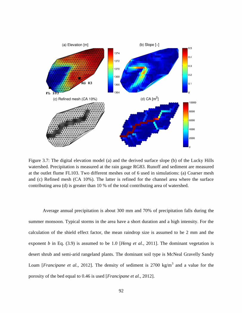
92

Figure 3.7: The digital elevation model (a) and the derived surface slope (b) of the Lucky Hills

watershed. Precipitation is measured at the rain gauge RG83. Runoff and sediment are measured

at the outlet flume FL103. Two different meshes out of 6 used in simulations: (a) Coarser mesh

and (c) Refined mesh (CA 10%). The latter is refined for the channel area where the surface

contributing area (d) is greater than 10 % of the total contributing area of watershed.

Average annual precipitation is about 300 mm and 70% of precipitation falls during the

summer monsoon. Typical storms in the area have a short duration and a high intensity. For the

calculation of the shield effect factor, the mean raindrop size is assumed to be 2 mm and the

exponent b in Eq. (3.9) is assumed to be 1.0 [Heng et al., 2011]. The dominant vegetation is

desert shrub and semi-arid rangeland plants. The dominant soil type is McNeal Gravelly Sandy

Loam [Francipane et al., 2012]. The density of sediment is 2700 kg/m3 and a value for the

porosity of the bed equal to 0.46 is used [Francipane et al., 2012].

93

The determination of the number of particle sizes (I) is of great importance for

representing size-selective characteristics. For this watershed, the particle size distributions

(PSDs) binned with 23 sieves (3, 6, 11, and 3 of them correspond to the range of clay, silt, sand,

and gravel, respectively) were collected at 6 different locations [Schaap and Shouse, 2003]. To

investigate the effects of the number of particle sizes on the generated sediment yields (SYs), the

averaged distributions for 6 locations with 23 intervals are recomputed into those with 4, 8, and

12 intervals (Figure 3.8). As shown in Figure 3.9-(a), the ratio of sediment yields with respect to

those obtained in the case with 23 intervals implies that the rough representation of PSD gives

rise to considerable variations (e.g., up to ~60 % for SY of sand). However, since the ratio of SY

of the finer particles is much greater than that of the coarser particles, the total SYs for 4 different

Is do not vary significantly (e.g., up to ~5 % for I = 4). Consequently, the PSD with 8 intervals is,

for efficiency, employed as the initial bed condition in the rest of simulations. The sediment size

of each interval is 0.001191, 0.002687, 0.01555, 0.04469, 0.2876, 1.131, 3.399, and 5 mm,

respectively; their corresponding fractions are 6.87, 3.33, 5.42, 4.77, 21.54, 18.39, 20.90, and

18.78 %; their settling velocities, , 0.0009823, 0.005001, 0.1669, 1.352, 32.89, 124.3,

252.2, and 313.6 mm/s, are calculated using the formula of Cheng [1997].

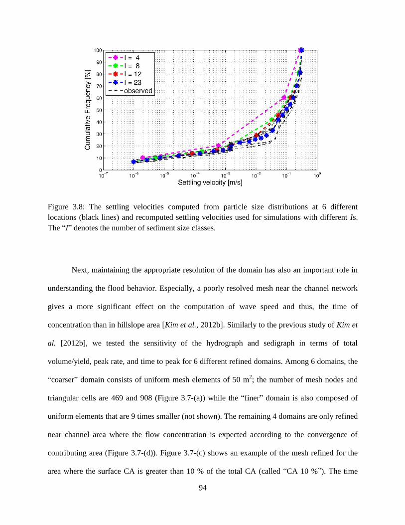
94

Figure 3.8: The settling velocities computed from particle size distributions at 6 different

locations (black lines) and recomputed settling velocities used for simulations with different Is.

The “I” denotes the number of sediment size classes.

Next, maintaining the appropriate resolution of the domain has also an important role in

understanding the flood behavior. Especially, a poorly resolved mesh near the channel network

gives a more significant effect on the computation of wave speed and thus, the time of

concentration than in hillslope area [Kim et al., 2012b]. Similarly to the previous study of Kim et

al. [2012b], we tested the sensitivity of the hydrograph and sedigraph in terms of total

volume/yield, peak rate, and time to peak for 6 different refined domains. Among 6 domains, the

“coarser” domain consists of uniform mesh elements of 50 m2; the number of mesh nodes and

triangular cells are 469 and 908 (Figure 3.7-(a)) while the “finer” domain is also composed of

uniform elements that are 9 times smaller (not shown). The remaining 4 domains are only refined

near channel area where the flow concentration is expected according to the convergence of

contributing area (Figure 3.7-(d)). Figure 3.7-(c) shows an example of the mesh refined for the

area where the surface CA is greater than 10 % of the total CA (called “CA 10 %”). The time

95

step used for hydrologic components is 3.75 min; the time step used for the simulation of flow

hydrodynamics and erosion-transport modeling components is 0.01 sec. Figure 3.9-(b) shows the

sensitivity through the ratio of several variables of 6 domains with respect to the coarser mesh.

CPU time is, as expected, more consumed as the number of cells/nodes increases; for the coarser

mesh, it takes 15850 sec to simulate a 3 hours rainfall event with a machine having an Intel Xeon

CPU (3.33 GHz, 2 processors) with 14 GB RAM. In contrast, the accuracy of the variables, i.e.,

total volume or total yield, peaks at hydrograph or sedigraph, and times to peaks is evaluated: for

the times to peak, results of all domains are consistent; the deviations of SY and peak at

sedigraph are up to 5 and 12 %, respectively, while those of flow volume and peak at hydrograph

are up to 1 and 2 %, respectively. It implies that sediment behaviors affected by more parameters

to be calibrated are more sensitive to the grid resolution than flow behaviors influenced by one

friction parameter. Hereafter, due to their small deviations, we will employ the coarser domain

with the time step of 0.1 sec for efficiency in the rest of simulations.

96

Figure 3.9: Sensitivity tests to the number of particle sizes (I) and the resolution of domain on

hydraulic and morphologic behaviors: (a) the ratio of sediment yields of 4 different Is with

respect to that of I=23; (b) the ratio of several variables (see legend) of 6 different domains with

respect to those of the coarser domain.

An extensive data set on precipitation, runoff, and sediment yield has been collected at

WGEW since the middle 1950s (http://www.tucson.ars.ag.gov/dap/) [Goodrich et al., 2008;

Nichols et al., 2008; Stone et al., 2008]. Data since 1999, when precipitation and runoff data

collection program was updated with new sensors, are used in this study. Ten precipitation

events for which runoff and sediment data exist were chosen for calibration and verification of

the numerical model. These events are summarized in Table 3.3.

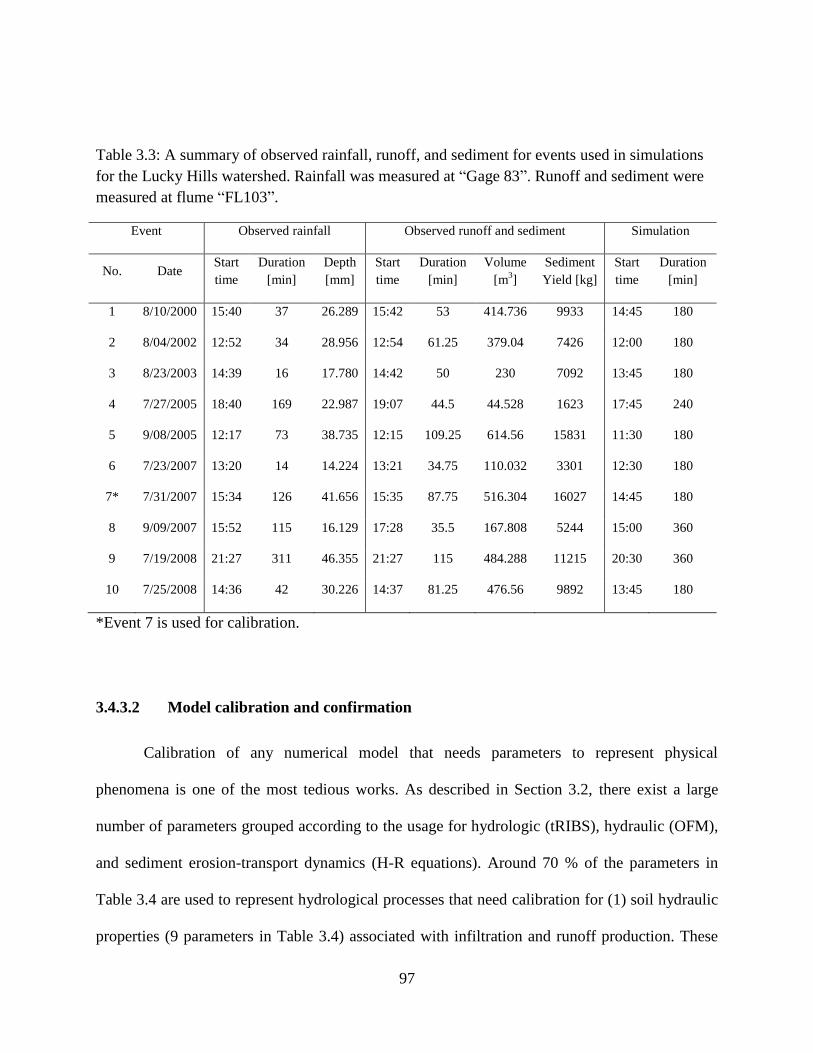
97

Table 3.3: A summary of observed rainfall, runoff, and sediment for events used in simulations

for the Lucky Hills watershed. Rainfall was measured at “Gage 83”. Runoff and sediment were

measured at flume “FL103”.

Event Observed rainfall Observed runoff and sediment Simulation

No. Date Start

time

Duration

[min]

Depth

[mm]

Start

time

Duration

[min]

Volume

[m3]

Sediment

Yield [kg]

Start

time

Duration

[min]

1 8/10/2000 15:40 37 26.289 15:42 53 414.736 9933 14:45 180

2 8/04/2002 12:52 34 28.956 12:54 61.25 379.04 7426 12:00 180

3 8/23/2003 14:39 16 17.780 14:42 50 230 7092 13:45 180

4 7/27/2005 18:40 169 22.987 19:07 44.5 44.528 1623 17:45 240

5 9/08/2005 12:17 73 38.735 12:15 109.25 614.56 15831 11:30 180

6 7/23/2007 13:20 14 14.224 13:21 34.75 110.032 3301 12:30 180

7* 7/31/2007 15:34 126 41.656 15:35 87.75 516.304 16027 14:45 180

8 9/09/2007 15:52 115 16.129 17:28 35.5 167.808 5244 15:00 360

9 7/19/2008 21:27 311 46.355 21:27 115 484.288 11215 20:30 360

10 7/25/2008 14:36 42 30.226 14:37 81.25 476.56 9892 13:45 180

*Event 7 is used for calibration.

3.4.3.2 Model calibration and confirmation

Calibration of any numerical model that needs parameters to represent physical

phenomena is one of the most tedious works. As described in Section 3.2, there exist a large

number of parameters grouped according to the usage for hydrologic (tRIBS), hydraulic (OFM),

and sediment erosion-transport dynamics (H-R equations). Around 70 % of the parameters in

Table 3.4 are used to represent hydrological processes that need calibration for (1) soil hydraulic

properties (9 parameters in Table 3.4) associated with infiltration and runoff production. These

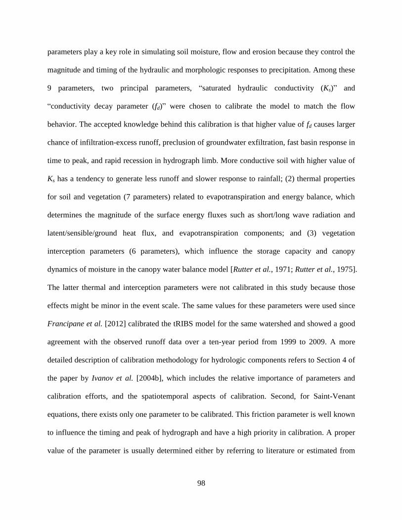
98

parameters play a key role in simulating soil moisture, flow and erosion because they control the

magnitude and timing of the hydraulic and morphologic responses to precipitation. Among these

9 parameters, two principal parameters, “saturated hydraulic conductivity (Ks)” and

“conductivity decay parameter (fd)” were chosen to calibrate the model to match the flow

behavior. The accepted knowledge behind this calibration is that higher value of fd causes larger

chance of infiltration-excess runoff, preclusion of groundwater exfiltration, fast basin response in

time to peak, and rapid recession in hydrograph limb. More conductive soil with higher value of

Ks has a tendency to generate less runoff and slower response to rainfall; (2) thermal properties

for soil and vegetation (7 parameters) related to evapotranspiration and energy balance, which

determines the magnitude of the surface energy fluxes such as short/long wave radiation and

latent/sensible/ground heat flux, and evapotranspiration components; and (3) vegetation

interception parameters (6 parameters), which influence the storage capacity and canopy

dynamics of moisture in the canopy water balance model [Rutter et al., 1971; Rutter et al., 1975].

The latter thermal and interception parameters were not calibrated in this study because those

effects might be minor in the event scale. The same values for these parameters were used since

Francipane et al. [2012] calibrated the tRIBS model for the same watershed and showed a good

agreement with the observed runoff data over a ten-year period from 1999 to 2009. A more

detailed description of calibration methodology for hydrologic components refers to Section 4 of

the paper by Ivanov et al. [2004b], which includes the relative importance of parameters and

calibration efforts, and the spatiotemporal aspects of calibration. Second, for Saint-Venant

equations, there exists only one parameter to be calibrated. This friction parameter is well known

to influence the timing and peak of hydrograph and have a high priority in calibration. A proper

value of the parameter is usually determined either by referring to literature or estimated from

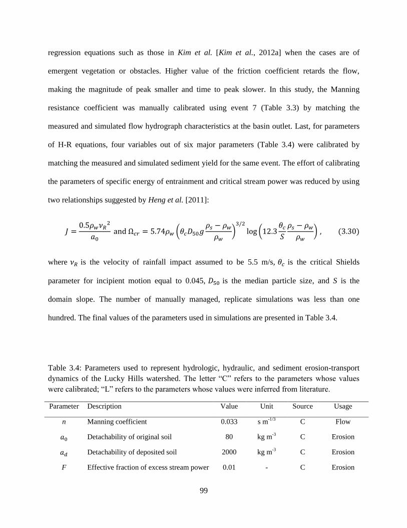
99

regression equations such as those in Kim et al. [Kim et al., 2012a] when the cases are of

emergent vegetation or obstacles. Higher value of the friction coefficient retards the flow,

making the magnitude of peak smaller and time to peak slower. In this study, the Manning

resistance coefficient was manually calibrated using event 7 (Table 3.3) by matching the

measured and simulated flow hydrograph characteristics at the basin outlet. Last, for parameters

of H-R equations, four variables out of six major parameters (Table 3.4) were calibrated by

matching the measured and simulated sediment yield for the same event. The effort of calibrating

the parameters of specific energy of entrainment and critical stream power was reduced by using

two relationships suggested by Heng et al. [2011]:

(

)

(

)

where is the velocity of rainfall impact assumed to be 5.5 m/s, is the critical Shields

parameter for incipient motion equal to 0.045, is the median particle size, and S is the

domain slope. The number of manually managed, replicate simulations was less than one

hundred. The final values of the parameters used in simulations are presented in Table 3.4.

Table 3.4: Parameters used to represent hydrologic, hydraulic, and sediment erosion-transport

dynamics of the Lucky Hills watershed. The letter “C” refers to the parameters whose values

were calibrated; “L” refers to the parameters whose values were inferred from literature.

Parameter Description Value Unit Source Usage

n Manning coefficient 0.033 s m-1/3

C Flow

Detachability of original soil

80 kg m-3

C Erosion

Detachability of deposited soil

2000 kg m-3

C Erosion

F Effective fraction of excess stream power

0.01 - C Erosion

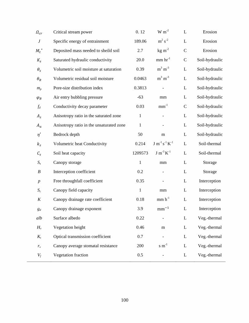
100

Critical stream power

0. 12 W m-2

L Erosion

J Specific energy of entrainment

189.06 m2 s

-2 L Erosion

Deposited mass needed to sheild soil

2.7 kg m

-2 C Erosion

Saturated hydraulic conductivity 20.0 mm hr-1

C Soil-hydraulic

Volumetric soil moisture at saturation 0.39 m3 m

-3 L Soil-hydraulic

Volumetric residual soil moisture 0.0463 m3 m

-3 L Soil-hydraulic

mp Pore-size distribution index 0.3813 - L Soil-hydraulic

Air entry bubbling pressure -63 mm L Soil-hydraulic

fd Conductivity decay parameter 0.03 mm-1

C Soil-hydraulic

Anisotropy ratio in the saturated zone 1 - L Soil-hydraulic

Anisotropy ratio in the unsaturated zone 1 - L Soil-hydraulic

Bedrock depth 50 m L Soil-hydraulic

Volumetric heat Conductivity 0.214 J m-1

s-1

K-1

L Soil-thermal

Soil heat capacity 1209573 J m-3

K-1 L Soil-thermal

Ss Canopy storage 1 mm L Storage

B Interception coefficient 0.2 - L Storage

p Free throughfall coefficient 0.35 - L Interception

Sc Canopy field capacity 1 mm L Interception

K Canopy drainage rate coefficient 0.18 mm h-1

L Interception

gd Canopy drainage exponent 3.9 L Interception

alb Surface albedo 0.22 - L Veg.-thermal

Hv Vegetation height 0.46 m L Veg.-thermal

Kt Optical transmission coefficient 0.7 - L Veg.-thermal

rs Canopy average stomatal resistance 200 s m-1

L Veg.-thermal

Vf Vegetation fraction 0.5 - L Veg.-thermal

101

By using the parameter values obtained through calibration for event 7, the total

watershed runoff volumes and sediment yields were calculated for ten selected events (Table 3.3).

The results were compared with observations and are shown in Figure 3.10. For relatively large

events, the simulated values tend to be overestimated, while for smaller events they are

somewhat underestimated. Despite these discrepancies, the comparison is very satisfactory: the

determination coefficients of R2=0.86 for runoff and R

2=0.80 for sediment were obtained (Figure

3.10). The discrepancies may be due to employed assumptions and inherent uncertainties: (1)

soil and land use characteristics used in tRIBS are assumed to be spatially uniform over the

entire basin; (2) precipitation is also assumed to be spatially uniform and data were aggregated to

a 15-minute resolution from a 1-minute resolution [Francipane et al., 2012], which may affect

runoff production; (3) the hydrological parameters were calibrated over a period of 10 years,

with the tendency of generating a slightly higher runoff for large events.

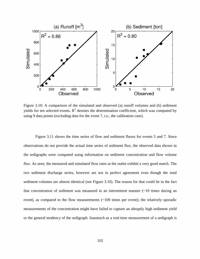
102

Figure 3.10: A comparison of the simulated and observed (a) runoff volumes and (b) sediment

yields for ten selected events. R2 denotes the determination coefficient, which was computed by

using 9 data points (excluding data for the event 7, i.e., the calibration case).

Figure 3.11 shows the time series of flow and sediment fluxes for events 5 and 7. Since

observations do not provide the actual time series of sediment flux, the observed data shown in

the sedigraphs were computed using information on sediment concentration and flow volume

flux. As seen, the measured and simulated flow rates at the outlet exhibit a very good match. The

two sediment discharge series, however are not in perfect agreement even though the total

sediment volumes are almost identical (see Figure 3.10). The reason for that could lie in the fact

that concentration of sediment was measured in an intermittent manner (~10 times during an

event), as compared to the flow measurements (~100 times per event); the relatively sporadic

measurements of the concentration might have failed to capture an abruptly high sediment yield

or the general tendency of the sedigraph. Inasmuch as a real-time measurement of a sedigraph is

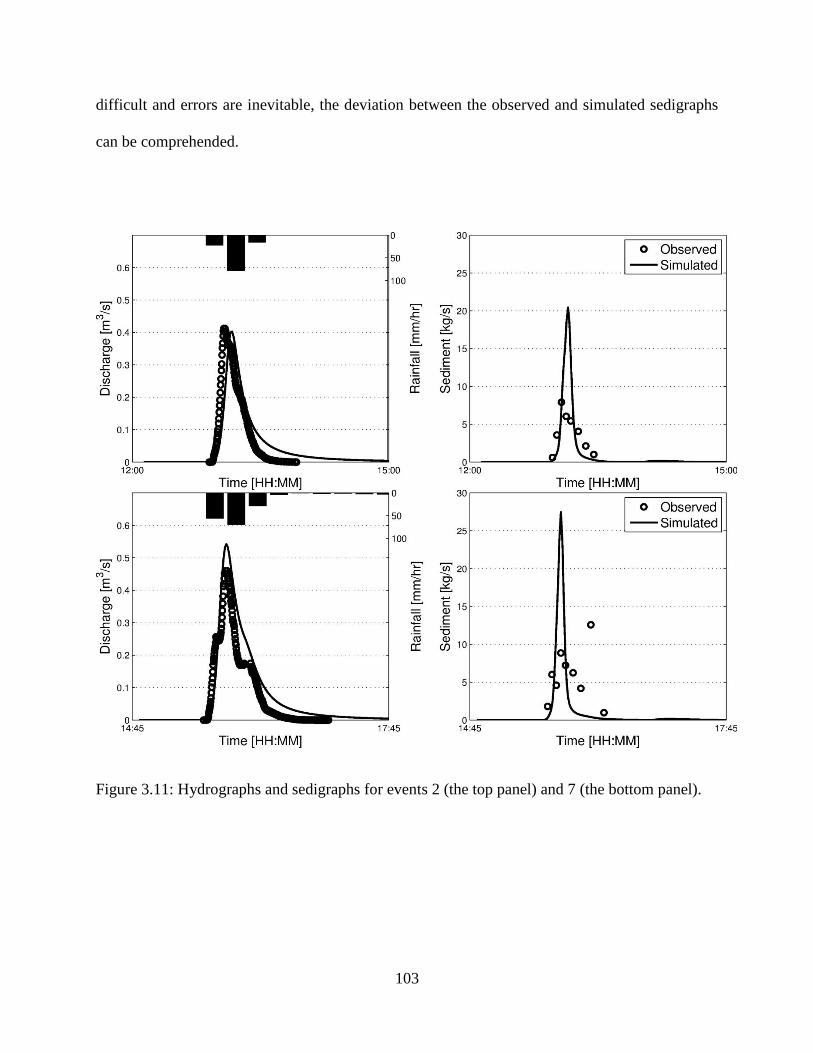
103

difficult and errors are inevitable, the deviation between the observed and simulated sedigraphs

can be comprehended.

Figure 3.11: Hydrographs and sedigraphs for events 2 (the top panel) and 7 (the bottom panel).

104

3.4.3.3 Spatial characteristics of flow and erosion processes

Figure 3.12 illustrates the simulated spatial distributions of depth, velocity, total

concentration, and elevation changes over the basin, and compares them at simulation hours 1

and 2 (event 7). The time of hour 1 corresponds to the occurrence of the observed peak and the

time of hour 2 corresponds to the recession period. As expected, higher depths, velocities, and

concentrations can be observed near the peak time, as compared to those during the recession

period. Elevation changes are such that most of the watershed area is being eroded, except for a

confluence area, where there is an abrupt morphological transition from steep to mild slopes

(Figures 3.7 and 3.12). Furthermore, sharp variations in the distributions of total concentration

(especially for the larger particles) and elevation change can be detected in that same area. In

order to address these variations from a mechanistic point of view, an inspection of the

governing equations for possible driving reasons is necessary.

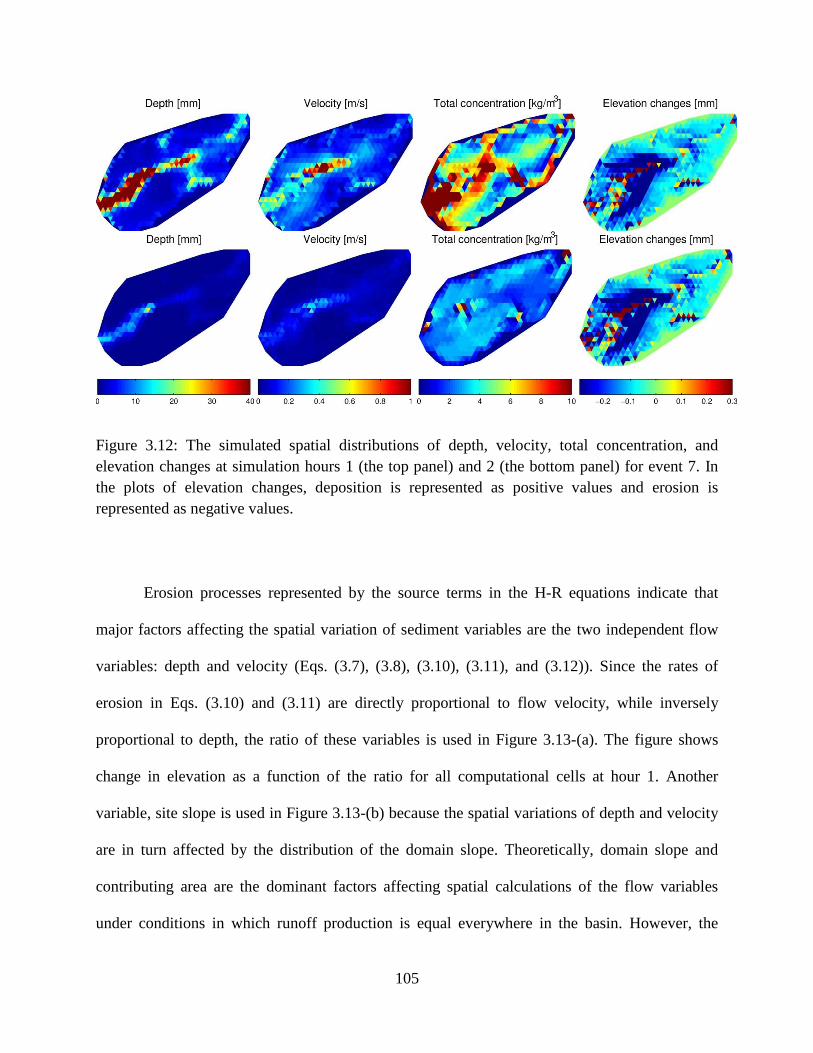
105

Figure 3.12: The simulated spatial distributions of depth, velocity, total concentration, and

elevation changes at simulation hours 1 (the top panel) and 2 (the bottom panel) for event 7. In

the plots of elevation changes, deposition is represented as positive values and erosion is

represented as negative values.

Erosion processes represented by the source terms in the H-R equations indicate that

major factors affecting the spatial variation of sediment variables are the two independent flow

variables: depth and velocity (Eqs. (3.7), (3.8), (3.10), (3.11), and (3.12)). Since the rates of

erosion in Eqs. (3.10) and (3.11) are directly proportional to flow velocity, while inversely

proportional to depth, the ratio of these variables is used in Figure 3.13-(a). The figure shows

change in elevation as a function of the ratio for all computational cells at hour 1. Another

variable, site slope is used in Figure 3.13-(b) because the spatial variations of depth and velocity

are in turn affected by the distribution of the domain slope. Theoretically, domain slope and

contributing area are the dominant factors affecting spatial calculations of the flow variables

under conditions in which runoff production is equal everywhere in the basin. However, the

106

effect of contributing area was not found to be significant in estimating the illustrated

morphological changes: a relationship between the elevation changes and the topographic index

exhibits a trend similar to that in Figure 3.13-(b) (not shown). Both plots in Figure 3.13 show

similar patterns of erosion dependence on a prognostic variable. Specifically, erosion is higher

for larger slopes (higher velocity, smaller depth). This indicates that in this zeroth-order

watershed, erosion is characteristic of “diffusive” mechanism, rather than fluvial erosion

[Istanbulluoglu et al., 2008; Francipane et al., 2012]. Specifically, diffusive erosion increases

with site slope, regardless of magnitude of contributing area, while fluvial erosion occurs in

channels where erosion scales with upstream contributing area. As seen in Figure 3.13-(b),

erosion dependence on site slope exhibits a threshold (~0.09 for slope) beyond which the

elevation changes grows significantly in a non-linear fashion. This behavior explains the

substantial changes of elevation observed in Figure 3.12 in the area of steep slopes. This result

indicates that topographic bed slope can be one of the most dominant factors in determining

erosion process in this watershed. Conversely, deposition is more likely to occur as the ratio of

flow velocity to depth or site slope decreases. But any generalization is difficult because

deposition does not occur frequently in this basin (~8% of the domain).

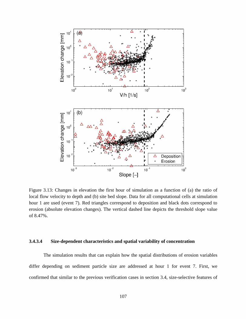
107

Figure 3.13: Changes in elevation the first hour of simulation as a function of (a) the ratio of

local flow velocity to depth and (b) site bed slope. Data for all computational cells at simulation

hour 1 are used (event 7). Red triangles correspond to deposition and black dots correspond to

erosion (absolute elevation changes). The vertical dashed line depicts the threshold slope value

of 8.47%.

3.4.3.4 Size-dependent characteristics and spatial variability of concentration

The simulation results that can explain how the spatial distributions of erosion variables

differ depending on sediment particle size are addressed at hour 1 for event 7. First, we

confirmed that similar to the previous verification cases in section 3.4, size-selective features of

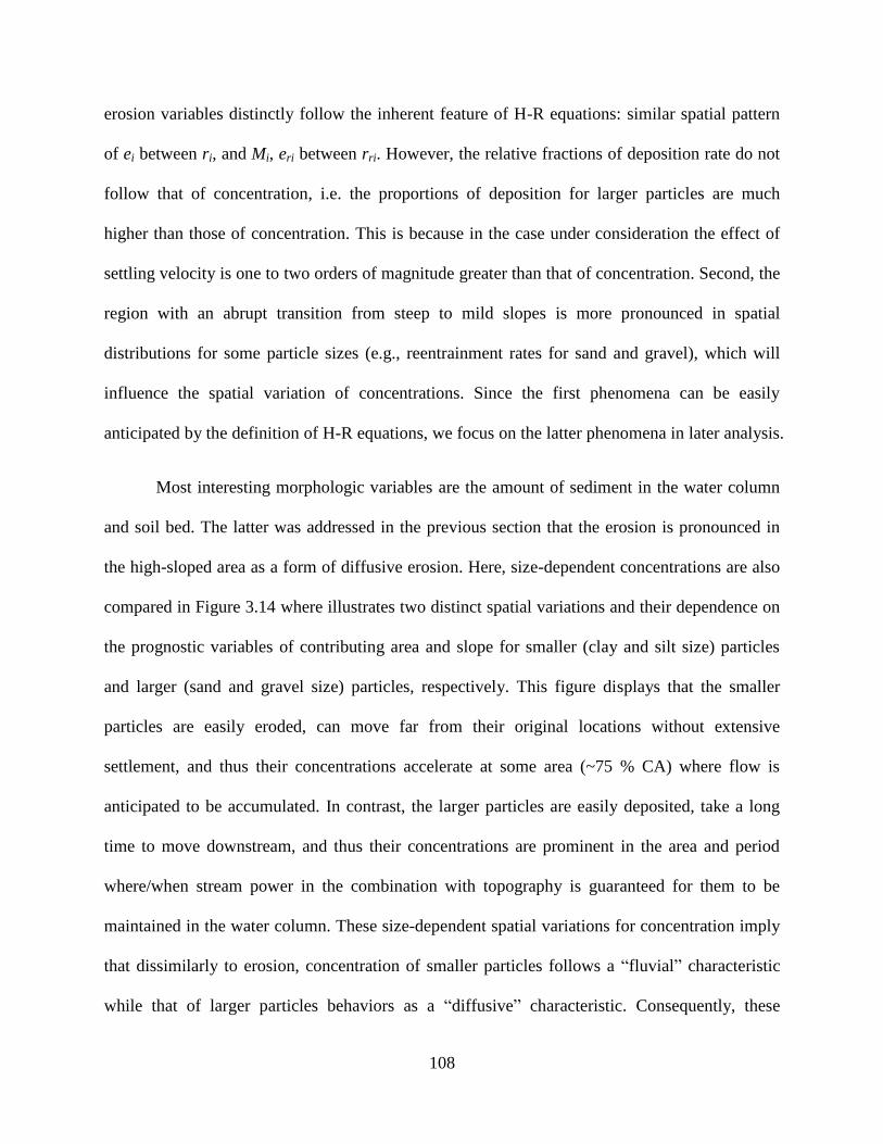
108

erosion variables distinctly follow the inherent feature of H-R equations: similar spatial pattern

of ei between ri, and Mi, eri between rri. However, the relative fractions of deposition rate do not

follow that of concentration, i.e. the proportions of deposition for larger particles are much

higher than those of concentration. This is because in the case under consideration the effect of

settling velocity is one to two orders of magnitude greater than that of concentration. Second, the

region with an abrupt transition from steep to mild slopes is more pronounced in spatial

distributions for some particle sizes (e.g., reentrainment rates for sand and gravel), which will

influence the spatial variation of concentrations. Since the first phenomena can be easily

anticipated by the definition of H-R equations, we focus on the latter phenomena in later analysis.

Most interesting morphologic variables are the amount of sediment in the water column

and soil bed. The latter was addressed in the previous section that the erosion is pronounced in

the high-sloped area as a form of diffusive erosion. Here, size-dependent concentrations are also

compared in Figure 3.14 where illustrates two distinct spatial variations and their dependence on

the prognostic variables of contributing area and slope for smaller (clay and silt size) particles

and larger (sand and gravel size) particles, respectively. This figure displays that the smaller

particles are easily eroded, can move far from their original locations without extensive

settlement, and thus their concentrations accelerate at some area (~75 % CA) where flow is

anticipated to be accumulated. In contrast, the larger particles are easily deposited, take a long

time to move downstream, and thus their concentrations are prominent in the area and period

where/when stream power in the combination with topography is guaranteed for them to be

maintained in the water column. These size-dependent spatial variations for concentration imply

that dissimilarly to erosion, concentration of smaller particles follows a “fluvial” characteristic

while that of larger particles behaviors as a “diffusive” characteristic. Consequently, these

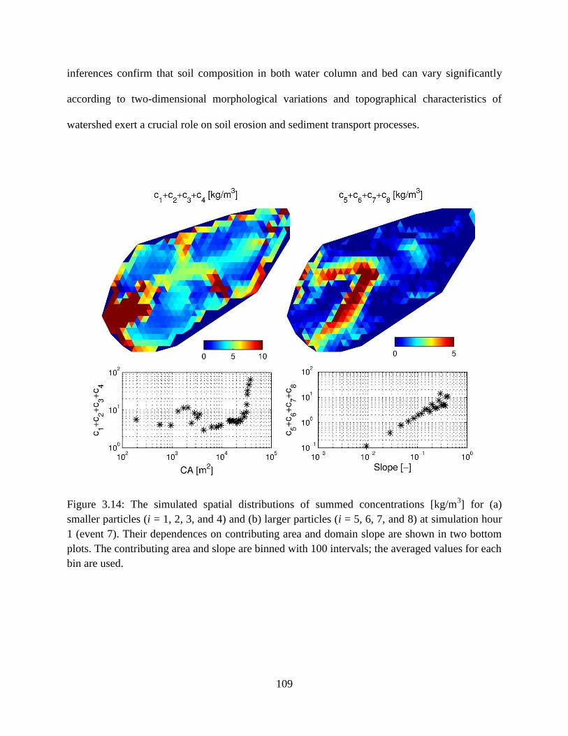
109

inferences confirm that soil composition in both water column and bed can vary significantly

according to two-dimensional morphological variations and topographical characteristics of

watershed exert a crucial role on soil erosion and sediment transport processes.

Figure 3.14: The simulated spatial distributions of summed concentrations [kg/m3] for (a)

smaller particles (i = 1, 2, 3, and 4) and (b) larger particles (i = 5, 6, 7, and 8) at simulation hour

1 (event 7). Their dependences on contributing area and domain slope are shown in two bottom

plots. The contributing area and slope are binned with 100 intervals; the averaged values for each

bin are used.

110

3.4.3.5 North- and south-facing characteristics of watershed system

Two critical features of watershed systems are their connectivity [Michaelides and

Chappell, 2009], i.e., hydrologically mediated transfer of mass, momentum, energy, or

organisms within or between basin compartments, and non-linear systems; their dynamics

depend on “convective” and “dissipative” characteristics of involved processes. In this section,

these connectivity and non-linearity between hydrologic processes, flow regime, erosion, and

stream sedimentation are addressed by investigating how disturbances arising at eco-

hydrological scale will necessarily propagate downstream. To introduce this perturbation, we

used the spatial distribution of mean annual biomass obtained from the simulations. Figure 3.15-

(a) evidently shows the effect of climate and slope aspect on vegetation that the north-facing

elements has a higher vegetation than the south-facing elements [Gutiérrez-Jurado et al., 2007].

We test two hypotheses in hydrologic and hydraulic viewpoints that the enhanced vegetation in

north-facing areas gives rise to less runoff production due to more infiltration, and flow

retardation caused by more obstacle effects. Two experimental heterogeneous cases as compared

to the control homogeneous case (event 7) are then designed: the first one is intended to have a

spatially distributed saturated conductivity ranging from 5 to 30 mm/hr such that the generated

runoff for different homogeneous conductivities lies in about 20 to 25 % variations [Gutiérrez-

Jurado et al., 2007]. The other heterogeneous case is designed to have a spatially distributed

Manning‟s coefficient ranging from 0.0265 to 0.0395 (note that 0.033 for the original

homogeneous case). The latter values are roughly estimated from the vegetation cover fraction

related to the mean annual biomass by using the Eq. (3.11) in Kim et al. [2012a].

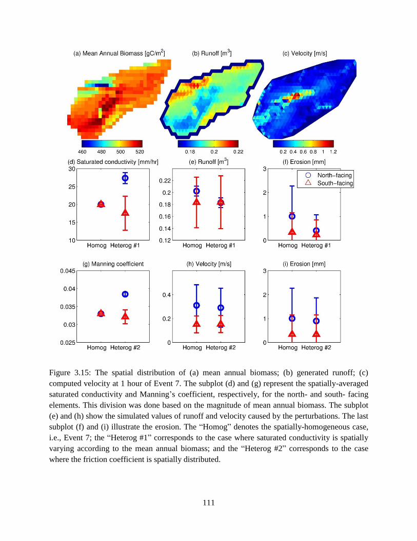
111

Figure 3.15: The spatial distribution of (a) mean annual biomass; (b) generated runoff; (c)

computed velocity at 1 hour of Event 7. The subplot (d) and (g) represent the spatially-averaged

saturated conductivity and Manning‟s coefficient, respectively, for the north- and south- facing

elements. This division was done based on the magnitude of mean annual biomass. The subplot

(e) and (h) show the simulated values of runoff and velocity caused by the perturbations. The last

subplot (f) and (i) illustrate the erosion. The “Homog” denotes the spatially-homogeneous case,

i.e., Event 7; the “Heterog #1” corresponds to the case where saturated conductivity is spatially

varying according to the mean annual biomass; and the “Heterog #2” corresponds to the case

where the friction coefficient is spatially distributed.

112

The hydrologic and hydraulic effects anticipated from these two heterogenetic variations

are illustrated in Figure 3.15-(b) and (c), respectively where runoff productions inversely follow

the biomass distribution and the velocity profile shows a slightly decrease on the north-facing

elements. These phenomena can be verified by quantitatively computing the spatially-averaged

values of runoff and velocity for south- and north- facing elements (Figure 3.15-(e) and (h)). The

corresponding erosion in north-facing area with more vegetation generally tends to decrease

resulting from reducing the runoff and velocity (Figure 3.15-(f) and (i)) while erosion in south-

facing area exhibits a minor deviation. Although these results are straightforwardly obtained

through two simple comparison tests, the tests are consequential in presenting a tool how the

basin system can be inevitably interacted with topography, soil, and vegetation acting on the

movement of flow and sediment. Another feature of this figure is non-linearity. For example,

~36 % increase of mean saturated conductivity in north-facing areas affects ~10 and 60 % of

reduction on runoff and erosion, respectively; ~16 % increase of mean Manning‟s coefficient in

the same area influences on the decrease of velocity and erosion by ~6 and 10 %. Despite of an

extensive number of other significant factors affecting on erosion at watershed scale, this

particular watershed addressed can sufficiently reveal a space-varying non-linearity according to

the initial condition of vegetation.

113

3.6 Summary

A novel two-dimensional, physically-based model of soil erosion and sediment transport

has been developed and coupled to a model that can simulate both hydrodynamic flow motions

and hydrologic surface and subsurface processes. The erosion and transport processes are

described with the Hairsine-Rose (H-R) model that accounts for size-selective sediment transport,

differentiates soil of the bed into original and deposited soil layers, and tracks in time the

development of the deposited area. The hydrologic and hydrodynamic model is tRIBS-OFM,

Triangulated irregular network – based, Real time Integrated Basin Simulator-Overland Flow

Model. For the solution of the combined two-dimensional, Saint-Venant and Hairsine-Rose

equations, the finite volume method is employed based on Roe‟s approximate Riemann solver

and resolved on an unstructured multiple resolution triangular mesh. The equations yielding

space-time dynamics of flow, erosion, and sediment transport thus represent a coupled system of

shallow water equations combined with advection-dominated transport equations for sediment of

multiple particle sizes.

The integrated model has been verified with analytical solutions and empirical data for

two one-dimensional benchmark cases dealing with rainfall-induced erosion and overland flow-

induced erosion. The size-selective results of spatial distributions of sediment concentrations and

deposited masses at different times, as well as temporal distributions, are presented and

demonstrate a good agreement with measured data.

The model has been consequently applied at catchment scale corresponding to the Lucky

Hills watershed located in southeastern Arizona, U.S.A. Before calibration, we performed a

sensitivity test to a grid resolution and the number of particle size. Then, model confirmation was

carried out for both flow volume and sediment yield at the basin outlet for ten different rainfall

114

events. As the simulation results indicate, a “diffusive” mode of erosion is characteristic of this

headwater, zeroth-order catchment: erosion increases with slope and is not greatly affected by

the contributing area. In particular, high elevation changes due to erosion occur over a limited

hillslope area where abrupt morphological changes exist: for slopes higher than ~0.09, the

elevation changes grow significantly in a non-linear fashion. In contrast, spatial, size-selective

characteristics for concentrations appear to have two modes of “diffusive” for larger particles

and “fluvial” for smaller particles. This tendency for concentration can also be identified in the

distributions of size-selective concentrations on the prognostic variables of contributing area and

domain slope. The results confirm that topographic characteristics of the basin can be one of the

most dominant factors in determining the amount of sediment in water column and soil bed of

this watershed, mediated by the dynamic flow regime of depth and velocity.

This study builds on and expands previous research by using a coupled framework that

adapts the Hairsine-Rose model to watershed-scale simulations. The essential strengths of the

combined framework are as follows. (1) Hydrological and hydraulic characteristics as well as

particle size distribution, arguably the three most crucial elements among external and internal

factors for modeling erosion, are all simultaneously taken into consideration. (2) The model is

based on sound physical laws, which result in narrow ranges of the parameter values that are

theoretically measurable; satisfactory results can thus be obtained with calibration efforts. This

model attribute makes feasible a wider range of real-world, catchment-scale flow/erosion

problems. (3) The spatially distributed, detailed information on soil type, land use, and

topography is becoming more accurate and easily accessible. This generates the potential for

making modeling of earth-surface processes more credible. By incorporating these types of

information, the developed hydrologic-hydrodynamic-erosion coupled model can be used as an

115

assessment tool for quantitative evaluation of spatiotemporal erosion responses to imposed

scenarios of climate change, variations in land-use, soil, and vegetation types in small- to

medium-size basins.

116

CHAPTER IV

Hydraulic resistance to overland flow on surfaces

with partially submerged vegetation

4.1 Introduction

Hydraulic resistance to open-channel and overland flows is an important characteristic

that needs to be represented properly in modeling runoff, flood routing and inundation, and soil

erosion. Resistance estimation affects not only the accurate calculation of flow variables, such as

the water depth, velocity, and shear stress, but also the prediction of their derivative outcomes,

such as the time of concentration, flow distribution in a basin, the transport capacity, the total

sediment yield, etc. The resistance of a surface can be characterized with several hydraulic

roughness coefficients. The most widely used are the Manning roughness coefficient (n), the

Chezy resistance factor (C), and the Darcy-Weisbach friction factor (f). Manning‟s n is most

popular in hydrological and soil erosion models, while using the Darcy-Weisbach f is more

common than the other resistance formulations in experimental studies [Hessel et al., 2003].

Theoretically, hydraulic resistance can be divided into five components: surface (grain)

resistance, form resistance, wave resistance, rain resistance, and bed-mobility resistance

[Abrahams and Parsons, 1994; S X Hu and Abrahams, 2006; M W Smith et al., 2007].

117

Numerous studies have performed field or laboratory experiments and theoretical

analyses seeking ways to relate hydraulic characterization of flow to roughness coefficients.

These studies tried to investigate a number of dimensionless variables in an attempt to find

suitable relationships using various metrics such as the Reynolds number (Re), the Froude

number (Fr), the characteristic roughness length (e.g., the ratio of depth to roughness element),

domain slope (S), and vegetation or obstacle cover fractions. Since early studies of overland flow,

resistance was described by a roughness coefficient, in analogy to the resistance relations used to

characterize flows in pipes. A relationship between the roughness coefficients and the Reynolds

number (e.g., f-Re) has been well established for shallow overland flows as well as for flows in

pipes and smooth channels [Chow, 1959; Emmett, 1970; R M Li and Shen, 1973; Phelps, 1975;

Savat, 1980]. The f-Re relationship has a negative slope of 1.0 in the laminar flow regime

[Blasius, 1913]; in turbulent flow, different f - Re relationships are obtained, depending on the

value of the relative roughness [Nikuradse, 1933]. These findings indicated that among several

possible dimensionless variables, Re has a predominant effect in quantifying the flow resistance

in conditions where the flow completely submerges a plane bed with either a smooth or a rough

surface. In such conditions, the roughness height is significantly smaller than the flow depth and

the hydraulic resistance is dominated by the surface resistance component arising due to the

presence of roughness elements beneath the flow surface.

However, in conditions where the surface is covered by stones, organic litter, or stems of

vegetation that protrude through the flow, the aforementioned f-Re relationships are not

applicable. Other dimensionless variables (e.g., Fr, relative roughness height, vegetation cover,

etc.) may become more dominant, reflecting that the form and wave resistance can become the

primary components of the total flow resistance [Emmett, 1970; Roels, 1984; Abrahams et al.,

118

1986; Gilley and Finkner, 1991; Gilley et al., 1992b; P Hirsch, 1996; Lawrence, 1997; 2000;

Takken and Govers, 2000; S X Hu and Abrahams, 2006]. For example, Emmett [1970] was the

first to emphasize the importance of form resistance caused by microtopography, which can

significantly exceed the surface resistance. Roels [1984] and Abrahams et al. [1986] stated that

the standard f-Re relationship is not ubiquitous: the f-Re relationship can have a convex upward

or a negatively sloping power-law relation. These relationships can be attributed to the

progressive inundation of roughness elements, implying that the surface configuration of the

elements, and not just the flow state, becomes dominant in quantifying the resistance. Further,

Gilley and Finkner [1991] presented a regression equation for predicting f and n by including the

characteristic length scale, i.e., a “random roughness index” as the primary variable. Gilley et al.

[1992b] suggested that f is largely controlled by a measure of the gravel cover fraction. Hirsch

[1996] developed a flow resistance model that explained flow conditions when the fraction of

roughness elements was greater than 10% and Fr was greater than 0.5.

Recently, Lawrence [1997] further demonstrated the importance of other dimensionless

variables in conditions of emerging vegetation and other types of obstacles protruding through

the flow. Rather than using the Reynolds number, Lawrence [1997] advocated the use of the

inundation ratio, h/kr, as the ratio of the flow depth h to the characteristic height of roughness

elements kr. Lawrence [1997] identified distinct flow regimes, such as partial and marginal

inundation, and well-inundated flows, with various fractions of obstacles (hemispheres) placed in

the flow. Depending on whether the flow depth h was greater/smaller than the characteristic

height kr, Lawrence [1997] estimated f as a function of the inundation ratio by using a drag

model for the partial inundation, a mixing length model for the marginal inundation, and a rough

turbulent flow formula for well-inundated flows. Since the estimation of the drag model showed

119

an underestimation of flow resistance for the partial inundation case, Lawrence [2000] later

modified the form drag model to obtain higher f values by increasing the drag coefficient, which

was negatively correlated with h/kr.

The modified model of Lawrence [2000] was successfully applied for the estimation of

flow resistance for the case of marginal inundation, where roughness elements were randomly

distributed and relatively uniform in size. However, when this model was applied under

conditions differing from the setting under which the model was developed, such as complex

flow geometries, the performance was not always satisfactory. Ferro [2003] tested the model

using laboratory measurements and showed that the modified mixing length formulation

provided accurate estimates, while the modified drag model resulted in a limited accuracy in

estimating f. Takken and Govers [2000] also tested the partial inundation case of Lawrence [1997]

and concluded that for situations with the complex configurations of roughness elements, a

single independent variable (i.e., h/kr) was insufficient to predict f. Thus, other variables, such as

the flow rate, Fr, and Re need to be considered to fully characterize the flow resistance [Takken

and Govers, 2000; Smart et al., 2002; S X Hu and Abrahams, 2006].

In shrubland or forested hillslopes, typical flow depths are much smaller than the height

of roughness elements such as vegetation stems and thus inundation ratios are very small. Such

flow conditions generally prevail in hillslope hydrological dynamics. Characterization of flow

for partially inundated conditions with a non-uniform distribution of roughness elements is

therefore significant for modeling runoff routing and soil erosion. However, these flow

conditions remain poorly characterized by empirical observations. For example, experimental

data from previous studies (see Fig. 4 in Lawrence [1997] reporting data from eleven studies) are

120

limited to partial inundation cases, i.e., most of the observed inundation ratios were between 0.1

and 1.

In order to establish a general relationship applicable to a wide range of conditions,

numerical modeling based on the two-dimensional shallow-water equations was carried out in

this study. The numerical simulations corresponded to overland flow on hillslopes covered with

shrubby or woody vegetation. An application of a numerical model, as compared to field or

experimental manipulations, provides several advantages. Specifically, in the case of small

depths of overland flow (few mm to cm length scale), the minimum requirement of water depth

for measuring the velocity with Acoustic Doppler velocimeters or electromagnetic current meters

is not satisfied [Lawless and Robert, 2001]. When the requirements are satisfied, small depths

still represent an issue in terms of measurement accuracy [Biron et al., 1998]. These difficulties

result in large measurement errors in laboratory or field experiments. Furthermore, the

determination of the friction (or energy) slope used in the calculation of roughness coefficients is

also cumbersome. It can be normally substituted with the bed slope under uniform flow

conditions, but it may not represent truthfully a spatially varying friction slope in situations with

many protruding obstacles. Lastly, the difficulty of controlling conditions for high flow rates

prevents empirical observations in field and laboratory studies [e.g., Takken and Govers, 2000;

Hessel et al., 2003]. For example, Takken and Govers [2000] used discharges ranging from

4.2 10-6

to 2.7 10-4

m3/s.

High-resolution, hydrodynamic numerical simulations can overcome all of the above

problems by specifying arbitrary flow conditions, including both high and low flow rates that

occur in real world situations. Using detailed simulations performed at fine space-time scales, the

properties of the resistance coefficient at larger spatial scales can be investigated. In order to

121

represent a system with tree/shrub stems, a sloped plane populated with “obstacle cells” that

have infinitely long vertical dimension was designed. A number of scenarios with different

domain slopes (S), inflow rates (Q), bed substrate roughness conditions ( ), and vegetation

cover fractions ( ) were considered. Based on the simulation results, two methods were

developed to obtain the upscaled Manning coefficient. A predictive equation was developed

using multiple regression and dimensional analyses and verified with five different experimental

data sets and a proposed wave resistance equation. Finally, the characteristic controls of several

independent variables on the roughness coefficient are described and evaluated.

4.2 Model suitability and simulation setup

4.2.1 Model suitability

The coupled model used is able to capture the phenomena of backwater and diverging-

converging thread as well as a noticeable change of flow variables (e.g., hydraulic jump). But,

one logical question is whether a simplified form of the Navier-Stokes equations, the Saint-

Venant shallow water equations, is an adequate approximation for simulating flows of relatively

small depth and flows passing in narrow openings between vegetation stems. Specifically, the

first possible concern is whether the S-V equations can accurately simulate very shallow flows.

Such flows can be affected by both bottom boundary layer and free surface movement, and the

vertically averaged S-V equations cannot recognize these effects of bottom/free surface

boundaries. However, the major assumption in applying the S-V equations is that depth (i.e., the

vertical direction scale) should be much smaller than the length scale of a flow phenomenon in

the horizontal direction. In an overland flow condition with small depths and a large spatial scale

122

of the domain, this assumption is quite acceptable. A second concern is whether the Manning‟s

parameterization used in the S-V equations can adequately capture the energy loss due to eddies

generated around plant stems. Three-dimensional turbulence modeling would appear to be a

more suitable method that can consider such effects and thus reduce the uncertainty of

simplifying assumptions of the S-V model. However, the application of turbulence models

presents a number of challenges. First, several parameters still need to be determined to close a

system of turbulence equations, e.g., k-epsilon, k-omega, SST, etc. for RANS models or

Smagorinsky constant in LES models. Second, in order to accurately resolve turbulent eddies,

appropriate representation scales have to be used and very fine mesh resolutions are necessary;

as a “rule of thumb”, mesh resolution has to be at least one order of magnitude finer than the

effective eddy scale. For example, Stoesser et al. [2010] used time steps satisfying the CFL

condition of 0.5 and a very fine mesh with nearly 30,000,000 grid points for a simulation case

with only 64 isolated stems. Although this study presented detailed results demonstrating various

turbulent characteristics, extending this approach to higher Reynolds numbers and randomly

distributed vegetation of a high cover fraction is not feasible. This would require much finer

space-time scales of representation.

4.2.2 Simulation setup

For the estimation of Manning‟s n for overland flow, numerical simulations are carried

out for an inclined plane that is 1 m wide and 2 m long, using slopes ranging from 10 to 110%

(5.7 to 47.7 degrees) at the 20% resolution of the slope. Such a range of bed slopes represents

possible hillslopes in a real watershed. The forcing for the domain is specified in two forms: as a

spatially uniform rainfall of 10 mm/hr continuous intensity over the entire duration of the

123

simulation and inflow rates of 0.0001, 0.0005, 0.001, and 0.01 m3/s uniformly distributed over

the width of the upstream boundary. The inflow rates were selected so as to describe a variety of

cases of hillslope hydrology. Specifically, the discharges of 0.0001, 0.001 and 0.01 m3/s

represent steady-state flow rates at different locations of a hypothetical 1-m wide planar slope at

10, 100, and 1000 m downstream of the upstream boundary, assuming 36 mm/hr excess rainfall

(e.g., the kinematic wave solution yields 0.0001 m3/s steady-state flow rate at the bottom of a 10

m hillslope as, etc.).

Manning‟s coefficients of 0.02, 0.03, and 0.04 were chosen so as to represent a bare,

rough plane surface without vegetation. These will be referred to as “the base Manning‟s

coefficients” and denoted by . The values of are used to represent various characteristics of

bed, such as the particle size and distribution, the roughness height, and the degree of tillage. For

example, a small value of corresponds to an experimental condition of bare sand, while a

larger value is a representation of the condition with irregular depressions and heavy protruding

stones. These constant base Manning coefficients only explain the resistance caused by friction

at the flow bottom and are within a range of values reported in literature.

Vegetation cover fractions (defined here as the fractional areas of non-submerged

“stems”, ) of 0, 5, 10, 20, 30, and 50% were used. The locations of vegetation stems were

determined randomly within the simulation domain for a given (see Figure 4.1). From a

computational standpoint, each stem of vegetation is represented as a rigid, infinitely-long wall

of hexagonal shape composed of six triangles. The shape can be fit within a circle that has a

diameter of approximately 2 cm. Since for most practical situations the order of depths

represented by the partial inundation is very small as compared to the stem height of plants, the

assumption of a rigid, infinitely-high wall is reasonable. The free-slip boundary condition is

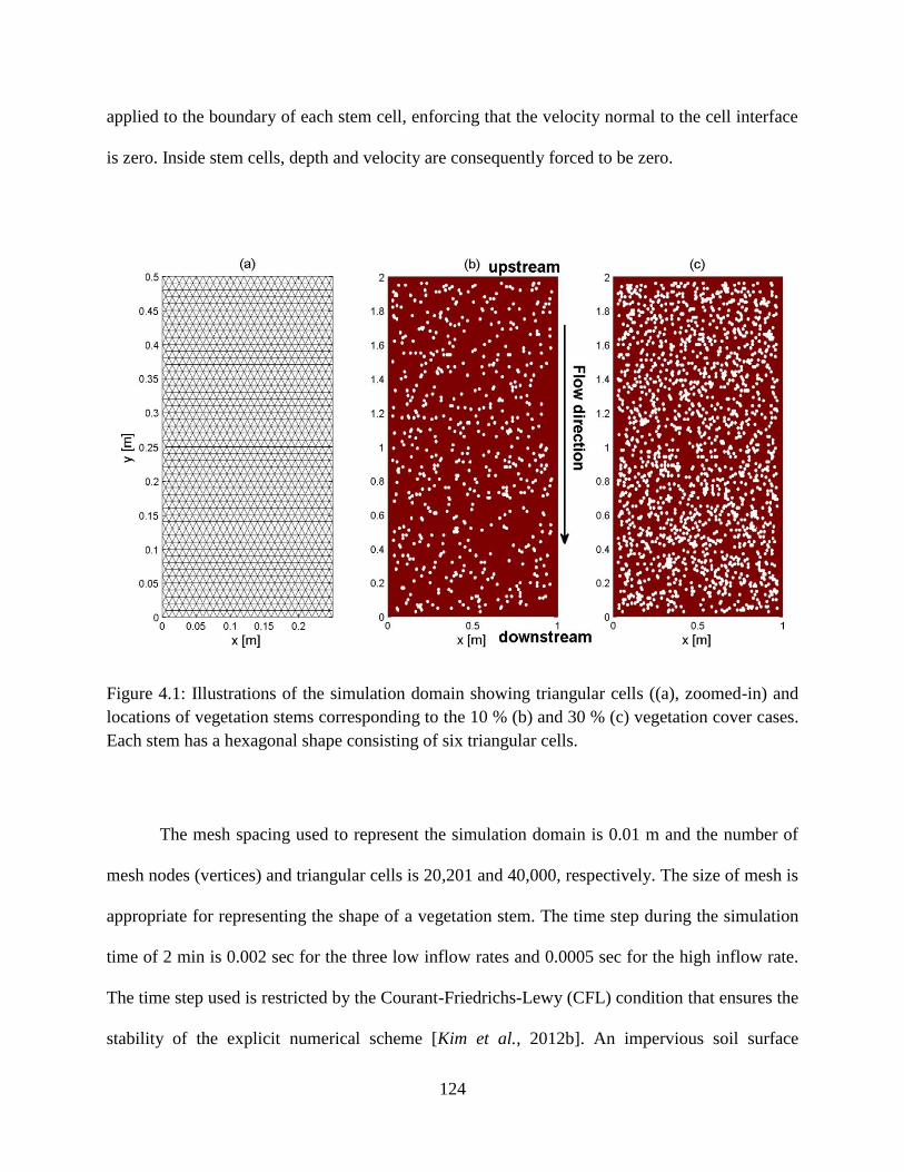
124

applied to the boundary of each stem cell, enforcing that the velocity normal to the cell interface

is zero. Inside stem cells, depth and velocity are consequently forced to be zero.

Figure 4.1: Illustrations of the simulation domain showing triangular cells ((a), zoomed-in) and

locations of vegetation stems corresponding to the 10 % (b) and 30 % (c) vegetation cover cases.

Each stem has a hexagonal shape consisting of six triangular cells.

The mesh spacing used to represent the simulation domain is 0.01 m and the number of

mesh nodes (vertices) and triangular cells is 20,201 and 40,000, respectively. The size of mesh is

appropriate for representing the shape of a vegetation stem. The time step during the simulation

time of 2 min is 0.002 sec for the three low inflow rates and 0.0005 sec for the high inflow rate.

The time step used is restricted by the Courant-Friedrichs-Lewy (CFL) condition that ensures the

stability of the explicit numerical scheme [Kim et al., 2012b]. An impervious soil surface

125

condition is assumed to exclude the processes of infiltration and subsurface flow. While the latter

impact surface runoff generation, the aim of the study is to investigate the effects of

unsubmerged obstacles on the flow process in conditions of clearly identifiable independent

variables; the impact of runoff-generating processes is indirectly accounted for through the

boundary inflow rate.

Simulation cases are designed so that the following characteristics are varied: vegetation

cover fraction ( ), plane slope (S), base Manning‟s coefficient ( ), and inflow rate (Q).

Preliminary simulations demonstrated that the effects of rainfall intensity were very minor, as

compared to an inflow rate. Therefore, only a single rainfall scenario (10 mm/hr) was used.

4.3 Methods for determining a representative value of resistance coefficient

This section describes methodologies of obtaining the upscaled values of the total surface

resistance ( ) based on the results of numerical simulations. Two methods for estimating , the

“Equivalent Roughness Surface” (ERS) and the “Equivalent Friction Slope” (EFS), are presented

in the following. The essential difference between the ERS and EFS methods is whether

information at internal data points is used for the computation of roughness, and the two methods

contain their advantages and disadvantages. As opposed to EFS, the ERS method does not

require any computations for the internal information but relies on a relationship between the

time of concentration of the flow and the Manning coefficient of a bare, rough plane surface

without vegetation for a given inflow rate and plane slope. The relationship should be

determined beforehand and thus additional simulations are necessary if a slope or a flow rate is

changed.

126

4.3.1 Equivalent Roughness Surface

One method to obtain an upscaled value of roughness is by using an “Equivalent

Roughness Surface” method. This method assumes that the resistance of a rough plane bed

without vegetation stems is equal to the resistance of a smooth plane covered with vegetation

stems. In other words, the effect of the form and wave resistances generated by internal obstacles

(i.e., stems in this study) is considered to exert the same effect as the surface resistance of a

rougher bed without vegetation. This method finds an equivalent resistance by analyzing the

hydrographs at an outlet region; specifically, it compares the times of concentration ( ) of the

simulated hydrographs for the flow case with vegetation stems and the case of flow over a rough,

bare soil plane without any unsubmerged obstacles. When is matched, the two hydrographs

corresponding to these flow situations are nearly identical.

The determination of corresponding to the simulated hydrographs plays a crucial role

in computing In this study, is defined as the time that satisfies the following two criteria:

where t is time; Q(t) is discharge at time t; is the theoretical discharge at steady-state,

equal to the upstream inflow rate plus the rainfall contribution; is a tolerance value assumed to

be in this study. The above criteria are chosen to avoid numerically unrealistic values in

estimation.

The derived relationship between and n (see section 4.4.2) was assumed to be linear

within intervals between the simulated cases. The relationship was used to find for any

arbitrary through interpolation. To make the assumption of linearity valid, numerous

127

simulations with small increments of n were performed for the bare plane conditions, spanning a

wide possible range of values.

4.3.2 Equivalent Friction Slope

The second method used in this study uses an “Equivalent Friction Slope”. It is based on

information simulated at internal points and computes an average value of resistance that

represents an upscaled value for the entire simulation domain. In order to obtain the value of n,

the Manning‟s equation is rearranged:

where is the hydraulic radius that can be replaced by the water depth, h, under the sheet flow

assumption; V is the flow velocity, calculated as √ ; u and v are x- and y- directional

depth-averaged velocities, respectively; is the friction slope. The energy slope is typically

replaced with the bottom slope for uniform flow. However, using the channel bottom slope is not

appropriate in the case when protruding vegetation or other obstacles exist. Thus, the

components of the friction slope are calculated as

(

√

)

(

√

)

128

where and are the x- and y- directional energy slope components; is the bed elevation;

g is the acceleration due to gravity; and, finally, is calculated as √

. The terms in

the above friction slope equations represent gravitational, pressure, and inertial forces,

respectively. Introducing a new variable, √

, its gradient can be calculated

numerically from the following equation:

∫

under the assumption that the gradient of is constant inside a triangle cell with an area of A.

When Green‟s theorem is applied in order to transform the area integral on the left-hand side of

equation (4.4) to a line integral, is integrated along the cell boundaries. Thus, the x-

directional friction slope becomes

( ) ( )

where the subscripts “0”, “1”, and “2” are used to denote the three counter-clockwise vertices of

a triangle cell [Kim et al., 2012b]. The y - directional component is obtained in a similar fashion.

Once the numerical model solves the mass and momentum equations of the flow, one can obtain

the primary flow variables such as h, u, and v at any point of the flow domain. Then, the

upscaled value of n for the entire domain can be computed by using the mean values of h, V, and

obtained at steady state:

129

where is the upscaled value of n; and are the means of depth and friction slope for all

triangle cells of the flow domain; is calculated by dividing the unit discharge (q) by the mean

depth ( ). This approach relies on an assumption that the representative value of for the whole

domain can be determined by averaging the corresponding local values. Since avoids negative

values because of the square root operation on the sum of its squared x- and y- components, it

does not loose information on the variability of local friction slopes; this would be the case if a

simple arithmetic averaging of negative and positive values were carried out.

4.4 Simulation results

4.4.1 Overall characterization of flow variables

Flow characteristics are first analyzed. Figure 4.2 shows the spatial distribution of

different flow variables such as depth, velocity, and friction slope at steady-state for the case of S

= 30%, = 0.02, and Q = 0.001 m3/s. The spatial distributions for the cases of bare soil and

vegetated soil with = 30% are compared. In the case of bare soil with these fairly large S and

Q, the flow approaches a uniform state with a depth of 0.0022 m and a velocity of 0.455 m/s.

These numerical values are also consistent with the results of the analytical steady uniform

equation for the “turbulent rough flow”, one of the four principal types of overland flow [Julien

and Simons, 1985]. Specifically, Manning‟s of 0.02 corresponds to a roughness height of mm

to cm scale (the mean diameter of sediment). This roughness height is much larger than the

thickness of the boundary sublayer, √ , and equal to 0.000144 m, which indicates

that the flow regime of this case is “turbulent rough”. Furthermore, the effects of inertia and

pressure terms are minimized and the bottom friction is balanced by the gravitational force. The

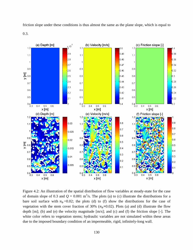
130

friction slope under these conditions is thus almost the same as the plane slope, which is equal to

0.3.

Figure 4.2: An illustration of the spatial distribution of flow variables at steady-state for the case

of domain slope of 0.3 and Q = 0.001 m3/s. The plots (a) to (c) illustrate the distributions for a

bare soil surface with =0.02; the plots (d) to (f) show the distributions for the case of

vegetation with the stem cover fraction of 30% ( =0.02). Plots (a) and (d) illustrate the flow

depth [m]; (b) and (e) the velocity magnitude [m/s]; and (c) and (f) the friction slope [-]. The

white color refers to vegetation stems; hydraulic variables are not simulated within these areas

due to the imposed boundary condition of an impermeable, rigid, infinitely-long wall.

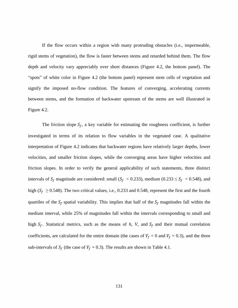
131

If the flow occurs within a region with many protruding obstacles (i.e., impermeable,

rigid stems of vegetation), the flow is faster between stems and retarded behind them. The flow

depth and velocity vary appreciably over short distances (Figure 4.2, the bottom panel). The

“spots” of white color in Figure 4.2 (the bottom panel) represent stem cells of vegetation and

signify the imposed no-flow condition. The features of converging, accelerating currents

between stems, and the formation of backwater upstream of the stems are well illustrated in

Figure 4.2.

The friction slope , a key variable for estimating the roughness coefficient, is further

investigated in terms of its relation to flow variables in the vegetated case. A qualitative

interpretation of Figure 4.2 indicates that backwater regions have relatively larger depths, lower

velocities, and smaller friction slopes, while the converging areas have higher velocities and

friction slopes. In order to verify the general applicability of such statements, three distinct

intervals of magnitude are considered: small ( < 0.233), medium (0.233 ≤ < 0.548), and

high ( ≥ 0.548). The two critical values, i.e., 0.233 and 0.548, represent the first and the fourth

quartiles of the spatial variability. This implies that half of the magnitudes fall within the

medium interval, while 25% of magnitudes fall within the intervals corresponding to small and

high . Statistical metrics, such as the means of h, V, and and their mutual correlation

coefficients, are calculated for the entire domain (the cases of = 0 and = 0.3), and the three

sub-intervals of (the case of = 0.3). The results are shown in Table 4.1.

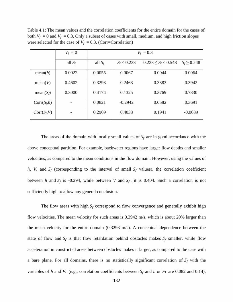
132

Table 4.1: The mean values and the correlation coefficients for the entire domain for the cases of

both Vf = 0 and Vf = 0.3. Only a subset of cases with small, medium, and high friction slopes

were selected for the case of Vf = 0.3. (Corr=Correlation)

Vf = 0 Vf = 0.3

all Sf all Sf Sf < 0.233 0.233 ≤ Sf < 0.548 Sf ≥ 0.548

mean(h) 0.0022 0.0055 0.0067 0.0044 0.0064

mean(V) 0.4602 0.3293 0.2463 0.3383 0.3942

mean(Sf) 0.3000 0.4174 0.1325 0.3769 0.7830

Corr(Sf,h) - 0.0821 -0.2942 0.0582 0.3691

Corr(Sf,V) - 0.2969 0.4038 0.1941 -0.0639

The areas of the domain with locally small values of are in good accordance with the

above conceptual partition. For example, backwater regions have larger flow depths and smaller

velocities, as compared to the mean conditions in the flow domain. However, using the values of

h, V, and (corresponding to the interval of small values), the correlation coefficient

between h and is -0.294, while between V and , it is 0.404. Such a correlation is not

sufficiently high to allow any general conclusion.

The flow areas with high correspond to flow convergence and generally exhibit high

flow velocities. The mean velocity for such areas is 0.3942 m/s, which is about 20% larger than

the mean velocity for the entire domain (0.3293 m/s). A conceptual dependence between the

state of flow and is that flow retardation behind obstacles makes smaller, while flow

acceleration in constricted areas between obstacles makes it larger, as compared to the case with

a bare plane. For all domains, there is no statistically significant correlation of with the

variables of h and Fr (e.g., correlation coefficients between and h or Fr are 0.082 and 0.14),

133

while weak correlation with the variables of V and Re (e.g., correlation coefficients between

and V or Re are 0.29 and 0.37) for vegetated hillslopes. These weak correlations make the

generalization or prediction of the degree of high variability of at any internal point difficult

and unfeasible. Therefore, the variability should be numerically modeled with a relevant detail in

estimating roughness coefficients for problems in which the value of is necessarily needed for

computations and plays a crucial role.

4.4.2 Results for the method of Equivalent Roughness Surface

Hydrographs at the downstream boundary of the domain were obtained for 324

simulations (as summarized in Table 4.2). They represent all possible permutations among 6

vegetation covers, 6 bed slopes, 3 base Manning coefficients, and 3 upstream boundary inflow

rates. Figure 4.3 shows 18 different hydrographs for fixed S and . Since overall trends shown

in Figure 4.3 look similar to the trends in the other 17 plots (not shown) with different S and ,

only one plot (Figure 4.3) out of 18 obtained plots is illustrated. The figure shows the

hydrographs for six different values of and three values of Q. The flow series with the same

peak discharge correspond to the cases with the same Q; the series with larger times of

concentration correspond to the cases with higher values. Based on these simulation results, it

can be concluded that as and increase, and Q and S decrease, flow retardation becomes

more pronounced, which results in higher values of .

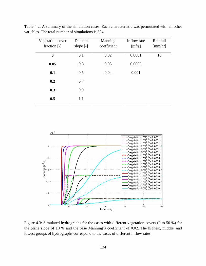
134

Table 4.2: A summary of the simulation cases. Each characteristic was permutated with all other

variables. The total number of simulations is 324.

Vegetation cover

fraction [-]

Domain

slope [-]

Manning

coefficient

Inflow rate

[m3/s]

Rainfall

[mm/hr]

0 0.1 0.02 0.0001 10

0.05 0.3 0.03 0.0005

0.1 0.5 0.04 0.001

0.2 0.7

0.3 0.9

0.5 1.1

Figure 4.3: Simulated hydrographs for the cases with different vegetation covers (0 to 50 %) for

the plane slope of 10 % and the base Manning‟s coefficient of 0.02. The highest, middle, and

lowest groups of hydrographs correspond to the cases of different inflow rates.

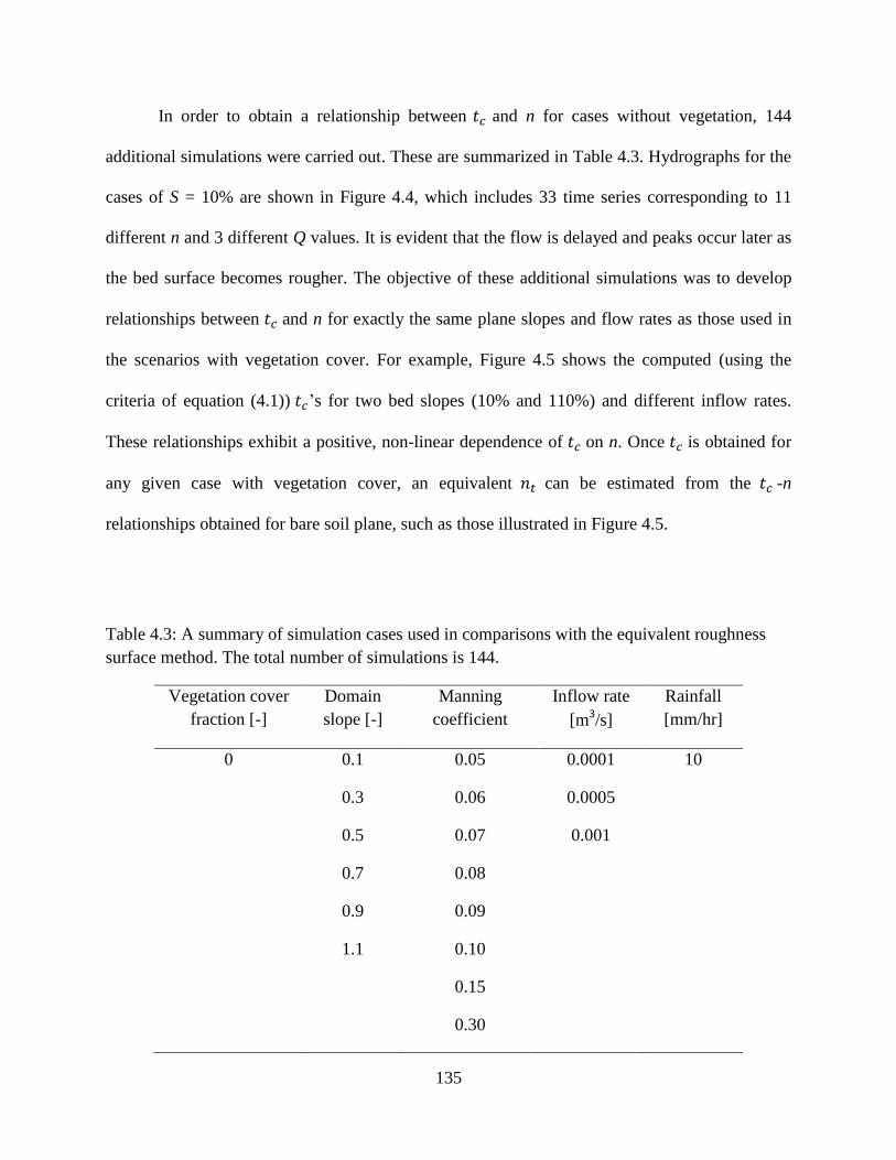
135

In order to obtain a relationship between and n for cases without vegetation, 144

additional simulations were carried out. These are summarized in Table 4.3. Hydrographs for the

cases of S = 10% are shown in Figure 4.4, which includes 33 time series corresponding to 11

different n and 3 different Q values. It is evident that the flow is delayed and peaks occur later as

the bed surface becomes rougher. The objective of these additional simulations was to develop

relationships between and n for exactly the same plane slopes and flow rates as those used in

the scenarios with vegetation cover. For example, Figure 4.5 shows the computed (using the

criteria of equation (4.1)) ‟s for two bed slopes (10% and 110%) and different inflow rates.

These relationships exhibit a positive, non-linear dependence of on n. Once is obtained for

any given case with vegetation cover, an equivalent can be estimated from the -n

relationships obtained for bare soil plane, such as those illustrated in Figure 4.5.

Table 4.3: A summary of simulation cases used in comparisons with the equivalent roughness

surface method. The total number of simulations is 144.

Vegetation cover

fraction [-]

Domain

slope [-]

Manning

coefficient

Inflow rate

[m3/s]

Rainfall

[mm/hr]

0 0.1 0.05 0.0001 10

0.3 0.06 0.0005

0.5 0.07 0.001

0.7 0.08

0.9 0.09

1.1 0.10

0.15

0.30

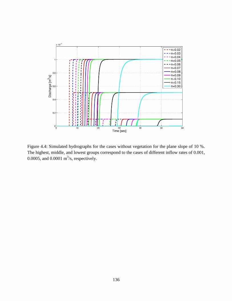
136

Figure 4.4: Simulated hydrographs for the cases without vegetation for the plane slope of 10 %.

The highest, middle, and lowest groups correspond to the cases of different inflow rates of 0.001,

0.0005, and 0.0001 m3/s, respectively.

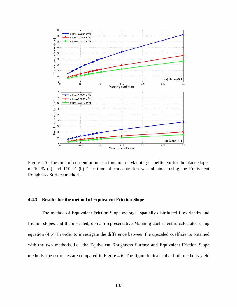
137

Figure 4.5: The time of concentration as a function of Manning‟s coefficient for the plane slopes

of 10 % (a) and 110 % (b). The time of concentration was obtained using the Equivalent

Roughness Surface method.

4.4.3 Results for the method of Equivalent Friction Slope

The method of Equivalent Friction Slope averages spatially-distributed flow depths and

friction slopes and the upscaled, domain-representative Manning coefficient is calculated using

equation (4.6). In order to investigate the difference between the upscaled coefficients obtained

with the two methods, i.e., the Equivalent Roughness Surface and Equivalent Friction Slope

methods, the estimates are compared in Figure 4.6. The figure indicates that both methods yield

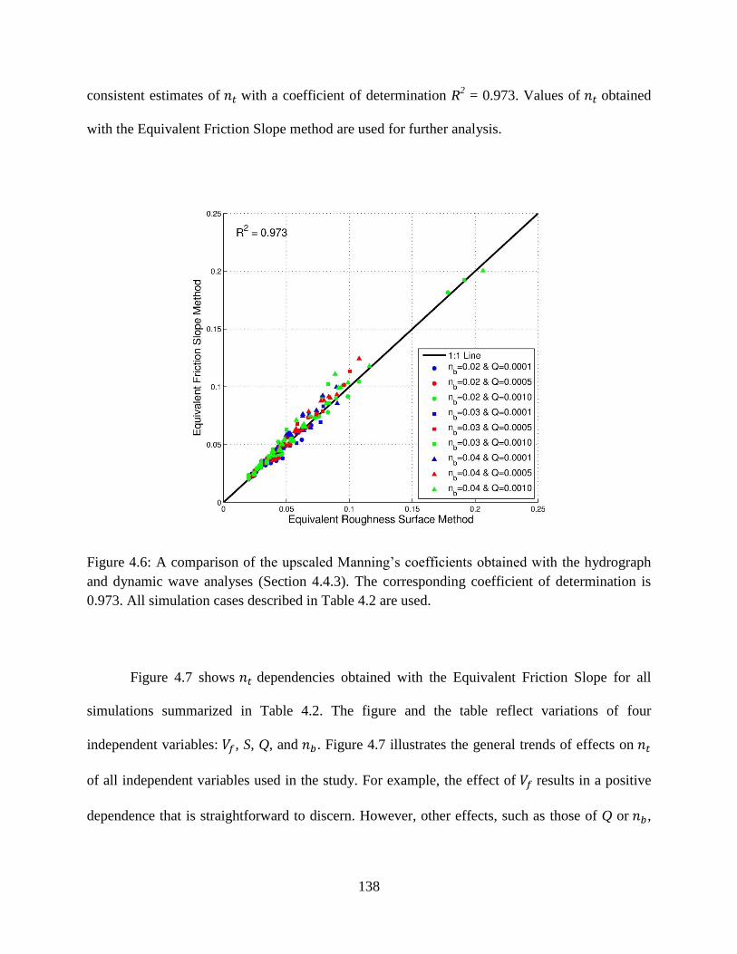
138

consistent estimates of with a coefficient of determination R2 = 0.973. Values of obtained

with the Equivalent Friction Slope method are used for further analysis.

Figure 4.6: A comparison of the upscaled Manning‟s coefficients obtained with the hydrograph

and dynamic wave analyses (Section 4.4.3). The corresponding coefficient of determination is

0.973. All simulation cases described in Table 4.2 are used.

Figure 4.7 shows dependencies obtained with the Equivalent Friction Slope for all

simulations summarized in Table 4.2. The figure and the table reflect variations of four

independent variables: , S, Q, and . Figure 4.7 illustrates the general trends of effects on

of all independent variables used in the study. For example, the effect of results in a positive

dependence that is straightforward to discern. However, other effects, such as those of Q or ,

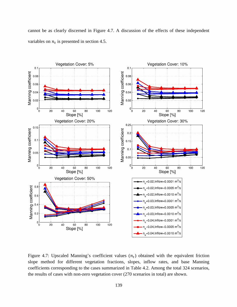
139

cannot be as clearly discerned in Figure 4.7. A discussion of the effects of these independent

variables on is presented in section 4.5.

Figure 4.7: Upscaled Manning‟s coefficient values ( ) obtained with the equivalent friction

slope method for different vegetation fractions, slopes, inflow rates, and base Manning

coefficients corresponding to the cases summarized in Table 4.2. Among the total 324 scenarios,

the results of cases with non-zero vegetation cover (270 scenarios in total) are shown.

140

4.4.4 Predictive equations for nt

The values of obtained from the Equivalent Friction Slope are used to develop

predictive equations for . The relevant predictive variables and their corresponding coefficients

are determined by using a dimensional analysis and a multiple linear regression.

Previous research has revealed that resistance to overland flow is influenced by many

factors. Among them are the Reynolds number, the Froude number, flow depth, vegetation cover

fraction, and the characteristics of roughness elements such as size, shape, spacing and pattern

[Abrahams and Parsons, 1994]. The effect of the inflow rate on the resistance is taken into

account by the Reynolds number. In this study, is assumed to be a function of the following

variables:

( )

where is the density of water [ML-3

]; is the dynamic viscosity of water [ML-1

T-1

]; g is the

acceleration due to gravity [LT-2

]. The Buckingham -theorem is used to select , , and since

these are repeating variables. The relevant dimensional parameters in the functional relation are

(

√ )

Since this predictive equation has been previously developed in the form of a power function [S

X Hu and Abrahams, 2006], equation (4.8) can be expressed in the following form:

(

)

(

√ )

( )

141

The term on the left side of this equation expresses the effect of vegetation on the total resistance

coefficient, i.e., it accounts for the contributions of both the form and wave resistances. The first

term on the right side is multiplied by 4 to represent the Reynolds number and the second term

represents the Froude number. The domain-averaged values of depth and velocity are used in the

regression. The kinematic viscosity is used as a constant with the value of 10-6

[m2/s], which

corresponds to the temperature of water of about 20°C. The evaluated coefficients a, b, c, d, and

e are 0.0264, 0.2794, -0.9859, 0.3060, and 0.9591, respectively, with =0.976 of the log-linear

form. Note that this regression equation was developed for the cases used in the simulations that

exhibit a wide range of possible scenarios of overland flow, i.e., and

.

As opposed to using all four dimensionless variables in Eq. (4.9), the consideration of

only three dimensionless variables at a time can show the relative importance of the omitted

variable in the variation of . This procedure indicates that the exclusion of each variable

Re, Fr, S, and reduces the explained variation by 3.2, 7.2, 1.5, and 35.7%, respectively. Such a

result implies that is the most dominant parameter in the determination of . Thus, in an

effort of simplification, if one chooses only to be present in the regression equation, the

resulting form will be

( )

with R2=0.873 (for the log-linear form), i.e., log ( can account for about 87% variation in

log . Alternatively, if the regression equation is represented with an exponential

function, the equation is

142

with R2=0.918 (for the log-linear form), which signifies a slightly better predictive power than

Eq. (4.10).

A number of scenarios (Table 4.4) for the highest inflow rate, Q = 0.01 m3/s, were

introduced. The objective was to further investigate the effect of partially submerged obstacles

on resistance for flow conditions that represent an extreme range for natural hillslopes, i.e.,

highly infrequent. Another set of regression equations including simulation data for all of the

cases summarized in Tables 4.2 and 4.4 are reported. Adding simulation data for Q = 0.01 m3/s

to the regression set, Eq. (4.9) becomes

(

)

(

√ )

( )

with R2=0.969 (for the log-linear form) and has the range of applicability:

and . Additionally, Eq. (4.11) becomes

with R2=0.831 (for the log-linear form). The regression equations (4.11) and (4.13) confirm that

vegetation exerts a predominant effect on the roughness coefficient; therefore, the derived

equations can be useful for estimating the degree of vegetation effects, if information on other

significant variables is not readily available.

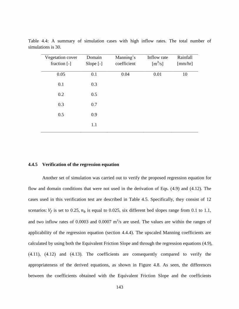
143

Table 4.4: A summary of simulation cases with high inflow rates. The total number of

simulations is 30.

Vegetation cover

fraction [-]

Domain

Slope [-]

Manning‟s

coefficient

Inflow rate

[m3/s]

Rainfall

[mm/hr]

0.05 0.1 0.04 0.01 10

0.1 0.3

0.2 0.5

0.3 0.7

0.5 0.9

1.1

4.4.5 Verification of the regression equation

Another set of simulation was carried out to verify the proposed regression equation for

flow and domain conditions that were not used in the derivation of Eqs. (4.9) and (4.12). The

cases used in this verification test are described in Table 4.5. Specifically, they consist of 12

scenarios: is set to 0.25, is equal to 0.025, six different bed slopes range from 0.1 to 1.1,

and two inflow rates of 0.0003 and 0.0007 m3/s are used. The values are within the ranges of

applicability of the regression equation (section 4.4.4). The upscaled Manning coefficients are

calculated by using both the Equivalent Friction Slope and through the regression equations (4.9),

(4.11), (4.12) and (4.13). The coefficients are consequently compared to verify the

appropriateness of the derived equations, as shown in Figure 4.8. As seen, the differences

between the coefficients obtained with the Equivalent Friction Slope and the coefficients

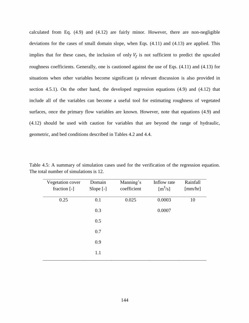
144

calculated from Eq. (4.9) and (4.12) are fairly minor. However, there are non-negligible

deviations for the cases of small domain slope, when Eqs. (4.11) and (4.13) are applied. This

implies that for these cases, the inclusion of only is not sufficient to predict the upscaled

roughness coefficients. Generally, one is cautioned against the use of Eqs. (4.11) and (4.13) for

situations when other variables become significant (a relevant discussion is also provided in

section 4.5.1). On the other hand, the developed regression equations (4.9) and (4.12) that

include all of the variables can become a useful tool for estimating roughness of vegetated

surfaces, once the primary flow variables are known. However, note that equations (4.9) and

(4.12) should be used with caution for variables that are beyond the range of hydraulic,

geometric, and bed conditions described in Tables 4.2 and 4.4.

Table 4.5: A summary of simulation cases used for the verification of the regression equation.

The total number of simulations is 12.

Vegetation cover

fraction [-]

Domain

Slope [-]

Manning‟s

coefficient

Inflow rate

[m3/s]

Rainfall

[mm/hr]

0.25 0.1 0.025 0.0003 10

0.3 0.0007

0.5

0.7

0.9

1.1

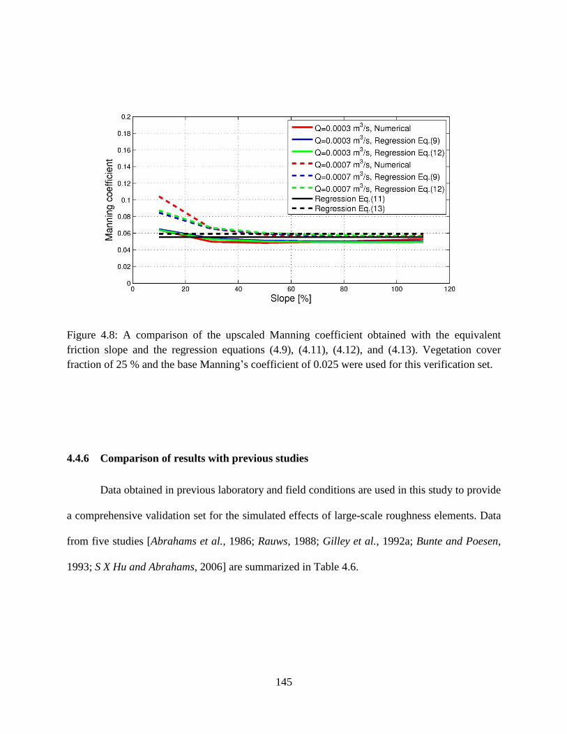
145

Figure 4.8: A comparison of the upscaled Manning coefficient obtained with the equivalent

friction slope and the regression equations (4.9), (4.11), (4.12), and (4.13). Vegetation cover

fraction of 25 % and the base Manning‟s coefficient of 0.025 were used for this verification set.

4.4.6 Comparison of results with previous studies

Data obtained in previous laboratory and field conditions are used in this study to provide

a comprehensive validation set for the simulated effects of large-scale roughness elements. Data

from five studies [Abrahams et al., 1986; Rauws, 1988; Gilley et al., 1992a; Bunte and Poesen,

1993; S X Hu and Abrahams, 2006] are summarized in Table 4.6.

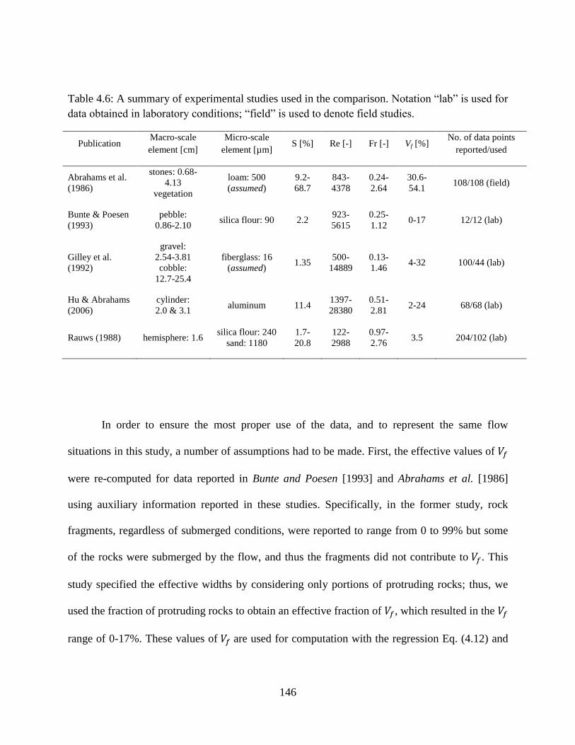
146

Table 4.6: A summary of experimental studies used in the comparison. Notation “lab” is used for

data obtained in laboratory conditions; “field” is used to denote field studies.

Publication Macro-scale

element [cm]

Micro-scale

element [µm] S [%] Re [-] Fr [-] Vf [%]

No. of data points

reported/used

Abrahams et al.

(1986)

stones: 0.68-

4.13

vegetation

loam: 500

(assumed)

9.2-

68.7

843-

4378

0.24-

2.64

30.6-

54.1 108/108 (field)

Bunte & Poesen

(1993)

pebble:

0.86-2.10 silica flour: 90 2.2

923-

5615

0.25-

1.12 0-17 12/12 (lab)

Gilley et al.

(1992)

gravel:

2.54-3.81

cobble:

12.7-25.4

fiberglass: 16

(assumed) 1.35

500-

14889

0.13-

1.46 4-32 100/44 (lab)

Hu & Abrahams

(2006)

cylinder:

2.0 & 3.1 aluminum 11.4

1397-

28380

0.51-

2.81 2-24 68/68 (lab)

Rauws (1988) hemisphere: 1.6 silica flour: 240

sand: 1180

1.7-

20.8

122-

2988

0.97-

2.76 3.5 204/102 (lab)

In order to ensure the most proper use of the data, and to represent the same flow

situations in this study, a number of assumptions had to be made. First, the effective values of

were re-computed for data reported in Bunte and Poesen [1993] and Abrahams et al. [1986]

using auxiliary information reported in these studies. Specifically, in the former study, rock

fragments, regardless of submerged conditions, were reported to range from 0 to 99% but some

of the rocks were submerged by the flow, and thus the fragments did not contribute to . This

study specified the effective widths by considering only portions of protruding rocks; thus, we

used the fraction of protruding rocks to obtain an effective fraction of , which resulted in the

range of 0-17%. These values of are used for computation with the regression Eq. (4.12) and

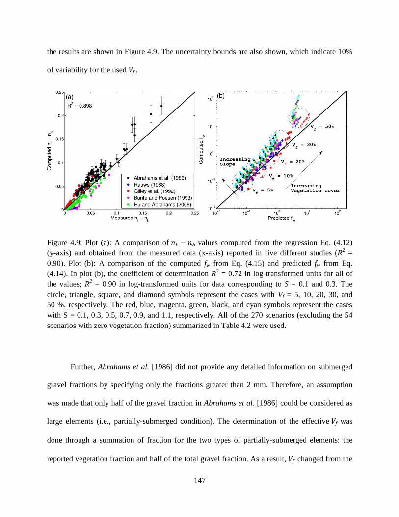
147

the results are shown in Figure 4.9. The uncertainty bounds are also shown, which indicate 10%

of variability for the used .

Figure 4.9: Plot (a): A comparison of values computed from the regression Eq. (4.12)

(y-axis) and obtained from the measured data (x-axis) reported in five different studies (R2 =

0.90). Plot (b): A comparison of the computed fw from Eq. (4.15) and predicted fw from Eq.

(4.14). In plot (b), the coefficient of determination R2 = 0.72 in log-transformed units for all of

the values; R2 = 0.90 in log-transformed units for data corresponding to S = 0.1 and 0.3. The

circle, triangle, square, and diamond symbols represent the cases with Vf = 5, 10, 20, 30, and

50 %, respectively. The red, blue, magenta, green, black, and cyan symbols represent the cases

with S = 0.1, 0.3, 0.5, 0.7, 0.9, and 1.1, respectively. All of the 270 scenarios (excluding the 54

scenarios with zero vegetation fraction) summarized in Table 4.2 were used.

Further, Abrahams et al. [1986] did not provide any detailed information on submerged

gravel fractions by specifying only the fractions greater than 2 mm. Therefore, an assumption

was made that only half of the gravel fraction in Abrahams et al. [1986] could be considered as

large elements (i.e., partially-submerged condition). The determination of the effective was

done through a summation of fraction for the two types of partially-submerged elements: the

reported vegetation fraction and half of the total gravel fraction. As a result, changed from the

148

originally reported range of 56.5-88.2% to 30.6-54.1%. Choosing the 50% ratio in order to get an

effective is an unavoidable assumption and thus it influences the computation of the resistance

coefficient. The sensitivity of estimates to this ratio is shown in the left plot of Figure 4.9: the

black dots correspond to the ratio of 50%, while the lower and upper bounds correspond to the

ratios of 40 and 60%, respectively. It is found that the effective rock ratio between 30% and 60%

shows a reasonable match with the predicted values with limited deviations from the one-to-one

regression line.

Further, Gilley et al. [1992b) specified flow depths that were larger than the dimension of

the gravel material; consequently, 36 data points for the gravel bed and 20 data points for the

cobble bed are excluded to avoid the submerged condition.

In the study by Rauws [1988], the depth range of 0.5 to 1.5 mm for the sub-experiment

performed over the sand bed has a similar order of magnitude as the dimensions of the micro-

scale sand bed (1.18 mm). In conditions of shallow flow over the sand bed, the effect of the

surface resistance induced by the sand bed may be much larger than that of the form/wave

resistances induced by the macro-scale roughness (only 3.5% of ), and thus data of the sand

bed experiment are also excluded from this analysis.

The objective of this study is to investigate the effects of large-scale elements on the total

resistance to flow. One way to carry out an analysis is to explore the fraction of the total

resistance ( ) in reference to the resistance caused by small-scale elements, i.e., with respect to

the surface resistance . The left plot in Figure 4.9 illustrates a comparison of

computed from the regression Eq. (4.12) and obtained from the reported data. It should be noted

that in all of the experimental studies, the value of was given, but the value of was not

149

provided in most studies, except for the work of Hu and Abrahams [2006]. Thus, the surface

resistance was derived based on auxiliary information provided for the small-scale roughness

elements. In order to derive reasonable approximations, the Strickler formula [Chow, 1959]

is used, where is the diameter of roughness elements in meters. We

assumed the diameter of micro-scale elements: 500 µm for loam in Abrahams et al. [1986] and

16 µm for fiberglass in Gilley et al. [1992]. We further found that the choice of the size of

roughness elements does not influence the determination of appreciably. Note that even

though several assumptions are made in the predicted , the overall deviations in this plot

are relatively minor (R2 = 0.898).

A comparison of data points computed based on the results of this study with the

estimates of the prognostic equation proposed by Hu and Abrahams [2006) is also presented.

Specifically, these authors computed flow resistance from their experimental data and proposed a

wave resistance ( ) formula for a fixed or mobile bed. The experiments were performed on a

flume that had the following characteristics: 0.5 m wide, 4.9 m long, slope of 0.114, covered

with cylinders with the diameters of 0.02 or 0.031 m (served as large-scale roughness elements).

The concentrations of cylinders ranged from 2 to 24%, and flows ranged from 0.000185 to

0.0034 m3/s. Hu and Abrahams [2006] first calculated the total roughness ( ), the surface

roughness ( ), and the form roughness ( ); they subsequently obtained by subtracting and

from . They presented a regression equation for a fixed bed as follows

(

)

where is the roughness Reynolds number, .

150

Using the flow variables obtained in this study, we can compute . Specifically, since

the effects of resistance due to rainfall and mobile bed on the total resistance are neglected, the

latter can be divided into three components assumed to be additive. Therefore, is calculated

with the following equation:

where the above three components on the right side of the equation are obtained from hydraulic

results based on the numerical simulations: ; can be substituted with

calculated for the case of a domain without vegetation; and is calculated by using the modified

drag model [Lawrence, 2000] for the case of partial inundation:

where accounts for the change in the frontal area with inundation, accounts for

the occluded volume of the roughness elements, and is the drag coefficient equal to 1.2,

which is the value used by Hu and Abrahams [2006]. The above formulation was originally

developed for roughness elements with a hemispheric shape. Thus, if we apply this for the

elements with the hexagonal column shape used in this study, we obtain ( )

and ( ) . Then, equation (4.16) becomes:

where is the area of the roughness element with the hexagonal shape. In order to verify the

simulated results, we compared computed from Eq. (4.15) (the y-axis in Figure 4.9b) with

151

predicted from Eq. (4.14) using the characteristics of flow scenarios of this study (the x-axis in

Figure 4.9b).

As Figure 4.9b shows, the results of applying Eq. (4.15) for and

are fairly consistent with the results obtained with Eq. (4.14) (R2=0.90 in log-transformed units),

while the results outside of these ranges are not, especially for the data with larger S and

. This can be partially attributed to the fact that the predictive equation (4.14) was

derived for the conditions of and , while this numerical study used

a much larger range of slope magnitudes and vegetation cover fractions. The plot exhibits two

discernible characteristics: first, an increasing vegetation cover implies an increase in wave

resistance (a straightforward and consistent conclusion following from Eq. (4.14)); second, the

higher the domain slope, the higher the differences between the compared values. The effect

of slope was not included in Eq. (4.14) developed by Hu and Abrahams [2006] because they

used a fixed domain slope, but, in general, it should be accounted for in the computation of .

4.5 Discussion

4.5.1 Effects of vegetation cover fraction

It is apparent from the simulation results that as increases, also grows. This

statement is also supported by the high values of the determination coefficient resulting from the

estimates obtained with Eqs. (4.11) and (4.13). Since in general hillslope flows have relatively

small discharges, (e.g., see Abrahams et al. [1986] for Walnut Gulch Experimental Watershed),

the results in cases presented in Table 4.2 are used in the following analysis. Figure 4.10 shows

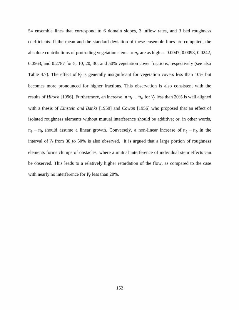
152

54 ensemble lines that correspond to 6 domain slopes, 3 inflow rates, and 3 bed roughness

coefficients. If the mean and the standard deviation of these ensemble lines are computed, the

absolute contributions of protruding vegetation stems to are as high as 0.0047, 0.0098, 0.0242,

0.0563, and 0.2787 for 5, 10, 20, 30, and 50% vegetation cover fractions, respectively (see also

Table 4.7). The effect of is generally insignificant for vegetation covers less than 10% but

becomes more pronounced for higher fractions. This observation is also consistent with the

results of Hirsch [1996]. Furthermore, an increase in for less than 20% is well aligned

with a thesis of Einstein and Banks [1950] and Cowan [1956] who proposed that an effect of

isolated roughness elements without mutual interference should be additive; or, in other words,

should assume a linear growth. Conversely, a non-linear increase of in the

interval of from 30 to 50% is also observed. It is argued that a large portion of roughness

elements forms clumps of obstacles, where a mutual interference of individual stem effects can

be observed. This leads to a relatively higher retardation of the flow, as compared to the case

with nearly no interference for less than 20%.

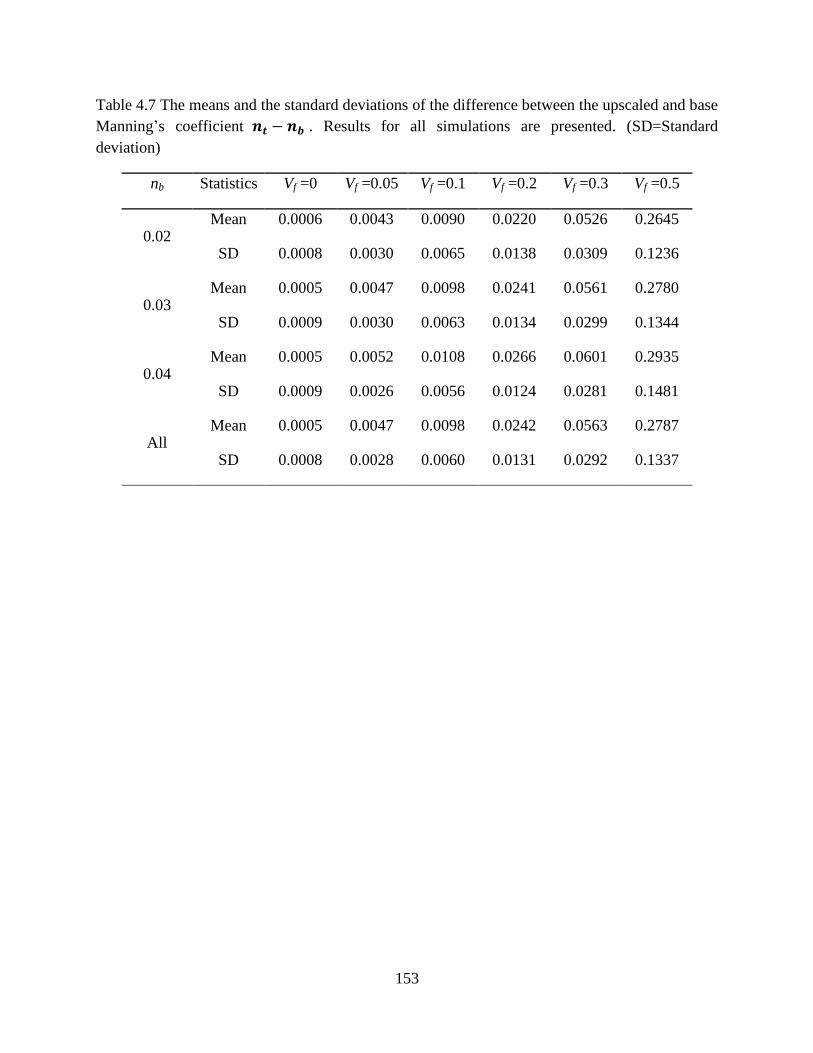
153

Table 4.7 The means and the standard deviations of the difference between the upscaled and base

Manning‟s coefficient . Results for all simulations are presented. (SD=Standard

deviation)

nb Statistics Vf =0 Vf =0.05 Vf =0.1 Vf =0.2 Vf =0.3 Vf =0.5

0.02 Mean 0.0006 0.0043 0.0090 0.0220 0.0526 0.2645

SD 0.0008 0.0030 0.0065 0.0138 0.0309 0.1236

0.03 Mean 0.0005 0.0047 0.0098 0.0241 0.0561 0.2780

SD 0.0009 0.0030 0.0063 0.0134 0.0299 0.1344

0.04 Mean 0.0005 0.0052 0.0108 0.0266 0.0601 0.2935

SD 0.0009 0.0026 0.0056 0.0124 0.0281 0.1481

All Mean 0.0005 0.0047 0.0098 0.0242 0.0563 0.2787

SD 0.0008 0.0028 0.0060 0.0131 0.0292 0.1337

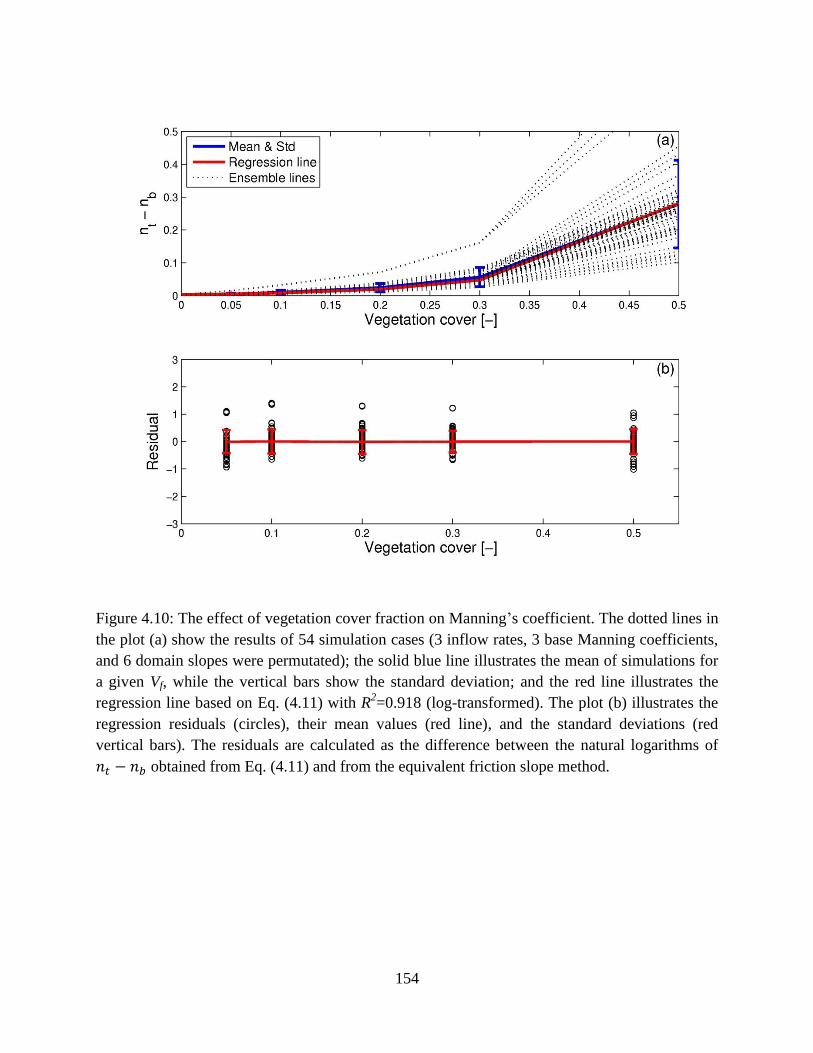
154

Figure 4.10: The effect of vegetation cover fraction on Manning‟s coefficient. The dotted lines in

the plot (a) show the results of 54 simulation cases (3 inflow rates, 3 base Manning coefficients,

and 6 domain slopes were permutated); the solid blue line illustrates the mean of simulations for

a given Vf, while the vertical bars show the standard deviation; and the red line illustrates the

regression line based on Eq. (4.11) with R2=0.918 (log-transformed). The plot (b) illustrates the

regression residuals (circles), their mean values (red line), and the standard deviations (red

vertical bars). The residuals are calculated as the difference between the natural logarithms of

obtained from Eq. (4.11) and from the equivalent friction slope method.

155

The residuals computed as the difference between the ensemble lines and the predicted

values from the regression equation (4.11) are calculated as the difference between the natural

logarithms of obtained from Eq. (4.11) and from the Equivalent Friction Slope method.

In the bottom plot of Figure 4.10, the mean of residuals at each is nearly zero and the standard

deviation of the residuals (in units of natural log-transform) is nearly constant. This ensures that

the regression equation (4.11) is a consistent estimator.

Equations (4.11) and (4.13) are derived only by considering the effects of vegetation

fraction. Regardless of what the values of the other variables are (e.g., Q or S), the values of

predicted with these equations are the same. Predictions may therefore contain large

errors in cases where the effects of Q and S become significant, and thus a caution should be

used in using these equations. In particular, cases with small S or high exhibit large effects of

Q and S, respectively. These are addressed in the following section.

4.5.2 Effects of bed slope

As Figure 4.7 shows, it is difficult to infer a unique trend of the resistance coefficient

relative to changes in S because may exhibit both negative and positive variations. The

negative trend of with growing S is characteristic for high flow rates, while a positive trend of

with increasing S can be discerned at low flow rates. These changes are relatively minor for

the cases with small vegetation cover. A positive trend with the domain slope at low flow rates

also emerged in the experimental study by Hessel et al. [2003], who used a discharge of about

6.67·10-5

m3/s. Their study used bed slopes less than 64%, a relatively small inflow rate, and

156

vegetation cover fractions smaller than ~30%. For a cropland area, they found an increase in

Manning‟s coefficient with increasing slope.

To further investigate possible trends, a set of simulation scenarios summarized in Table

4.4 were considered in addition to the cases described in Table 4.2. These included extreme cases

with a higher inflow rate of 0.01 m3/s. Flow rates reaching or exceeding such a magnitude are

unlikely to occur in real-world hillslopes, except for most extreme hydrologic events. The four

considered inflow rates, i.e., 0.0001, 0.0005, 0.001, and 0.01 m3/s, therefore span the likeliest

possible range and extend the analysis to “limiting” flow conditions. Similar to previous results

in Figure 4.7, the set of simulation cases for Q = 0.01 m3/s exhibit a decreasing trend of with

growing slope (not shown).

The effects of the difference in possible trends can be explained by using the Manning‟s

equation. For a given inflow rate, the spatial variability of is influenced by both friction slope

and depth:

If the plane slope is increased, the friction slope will also grow, and the flow depth will decrease.

These two effects exert a conflicting impact on the determination of and thus are the reason of

the two trends observed in the simulation results for changes in the bed slope. A specific trend

(i.e., the growth or decay of with S) is observed depending on whether the contribution of one

effect overwhelms the contribution of the other. Selecting 10% bed slope as a “reference” slope

and deriving the ratio of at any slope with respect to at this reference slope yields an

equation in a logarithmic form:

157

(

)

(

)

(

)

which implies that varies according to its controlling variables and . The three terms of

Eq. (4.19) are shown in Figure 4.11 for three different vegetation cover fractions of 0, 10, and

30%. For , the effects of and are nearly identical in the absolute magnitude and thus

is almost constant. However, for larger stem fractions (e.g., ), the gradient is

less than zero for larger inflow rates and nearly always positive for the smallest flow rate. The

latter effect is because the relative rate of increase of with respect to is higher than the

rate of decrease of with respect to ; the opposite holds true for the higher flow rates. One

can consequently infer that the gradient becomes zero or, equivalently, exhibits a local

minimum, where the two effects are balanced.

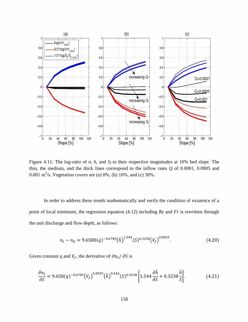
158

Figure 4.11: The log-ratio of n, h, and Sf to their respective magnitudes at 10% bed slope. The

thin, the medium, and the thick lines correspond to the inflow rates Q of 0.0001, 0.0005 and

0.001 m3/s. Vegetation covers are (a) 0%, (b) 10%, and (c) 30%.

In order to address these trends mathematically and verify the condition of existence of a

point of local minimum, the regression equation (4.12) including Re and Fr is rewritten through

the unit discharge and flow depth, as follows:

( )

( )

Given constant q and , the derivative of is

( )

( )

*

+

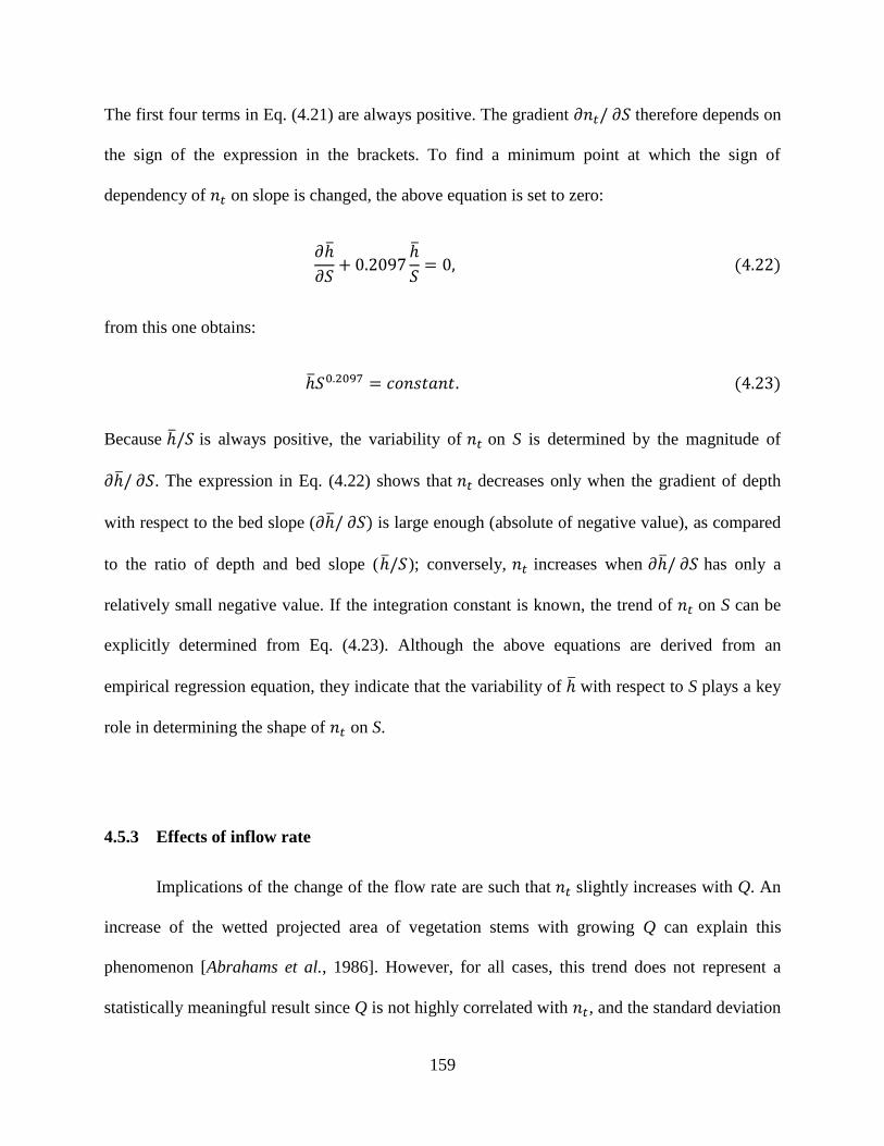
159

The first four terms in Eq. (4.21) are always positive. The gradient therefore depends on

the sign of the expression in the brackets. To find a minimum point at which the sign of

dependency of on slope is changed, the above equation is set to zero:

from this one obtains:

Because is always positive, the variability of on S is determined by the magnitude of

. The expression in Eq. (4.22) shows that decreases only when the gradient of depth

with respect to the bed slope ( is large enough (absolute of negative value), as compared

to the ratio of depth and bed slope ( ); conversely, increases when has only a

relatively small negative value. If the integration constant is known, the trend of on S can be

explicitly determined from Eq. (4.23). Although the above equations are derived from an

empirical regression equation, they indicate that the variability of with respect to S plays a key

role in determining the shape of on S.

4.5.3 Effects of inflow rate

Implications of the change of the flow rate are such that slightly increases with Q. An

increase of the wetted projected area of vegetation stems with growing Q can explain this

phenomenon [Abrahams et al., 1986]. However, for all cases, this trend does not represent a

statistically meaningful result since Q is not highly correlated with , and the standard deviation

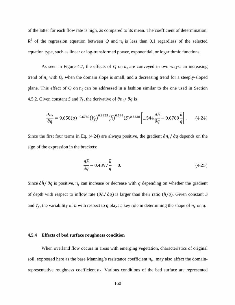
160

of the latter for each flow rate is high, as compared to its mean. The coefficient of determination,

R2 of the regression equation between Q and

is less than 0.1 regardless of the selected

equation type, such as linear or log-transformed power, exponential, or logarithmic functions.

As seen in Figure 4.7, the effects of Q on are conveyed in two ways: an increasing

trend of with Q, when the domain slope is small, and a decreasing trend for a steeply-sloped

plane. This effect of Q on can be addressed in a fashion similar to the one used in Section

4.5.2. Given constant S and , the derivative of is

( )

( )

*

+

Since the first four terms in Eq. (4.24) are always positive, the gradient depends on the

sign of the expression in the brackets:

Since is positive, can increase or decrease with q depending on whether the gradient

of depth with respect to inflow rate ( is larger than their ratio ( ). Given constant S

and , the variability of with respect to q plays a key role in determining the shape of on q.

4.5.4 Effects of bed surface roughness condition

When overland flow occurs in areas with emerging vegetation, characteristics of original

soil, expressed here as the base Manning‟s resistance coefficient , may also affect the domain-

representative roughness coefficient . Various conditions of the bed surface are represented

161

with different values of , e.g., a larger corresponds to a rougher condition of the bed. The

effect of on is illustrated in Figure 4.12 in which is used as the variable for the y-

axis. This difference can be also recognized as the net total contributions of the form and wave

resistances, which need to be accounted for in the presence of obstacles. Note that an analysis of

the effect of should be carried by mutually comparing the sets of lines of different color: red

( =0.04), black ( =0.02), and blue ( =0.03) lines (see Figure 4.12). The red lines are mostly

above the black lines, which implies that the rougher the surface of the plane, the larger the

effect of the form/wave resistances due to vegetation. As compared to the smoother bed

corresponding to of 0.02, the rougher bed with of 0.04 leads to increasing contributions of

the form/wave resistances to by about 21, 20, 21, 14, 11% for the vegetation cover of 5, 10,

20, 30, 50%, respectively (Table 4.7).

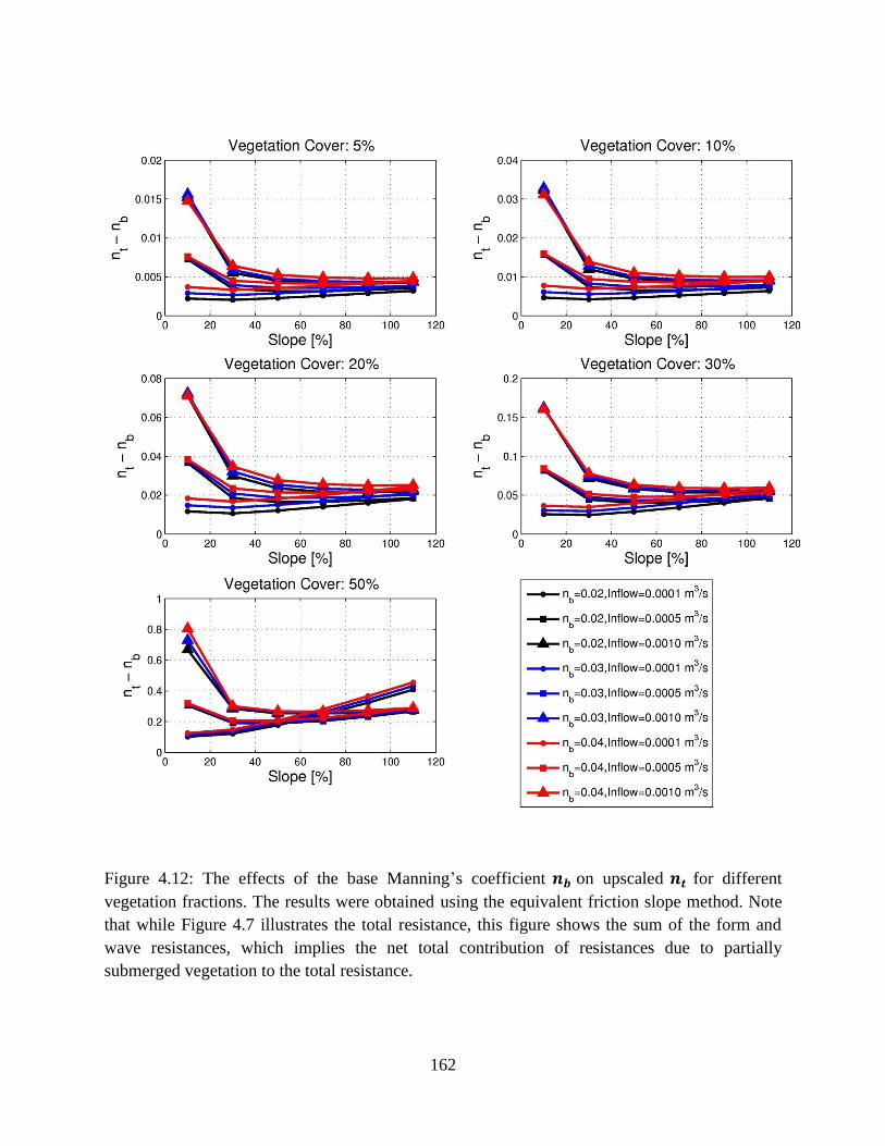
162

Figure 4.12: The effects of the base Manning‟s coefficient on upscaled for different

vegetation fractions. The results were obtained using the equivalent friction slope method. Note

that while Figure 4.7 illustrates the total resistance, this figure shows the sum of the form and

wave resistances, which implies the net total contribution of resistances due to partially

submerged vegetation to the total resistance.

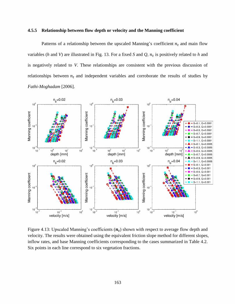
163

4.5.5 Relationship between flow depth or velocity and the Manning coefficient

Patterns of a relationship between the upscaled Manning‟s coefficient and main flow

variables (h and V) are illustrated in Fig. 13. For a fixed S and Q, is positively related to h and

is negatively related to V. These relationships are consistent with the previous discussion of

relationships between and independent variables and corroborate the results of studies by

Fathi-Moghadam [2006].

Figure 4.13: Upscaled Manning‟s coefficients ( ) shown with respect to average flow depth and

velocity. The results were obtained using the equivalent friction slope method for different slopes,

inflow rates, and base Manning coefficients corresponding to the cases summarized in Table 4.2.

Six points in each line correspond to six vegetation fractions.

164

4.5.6 Validity of performance skill

Despite the simplified nature of the S-V equations and the implications of underlying

assumptions, the results of this study are consistent with a broad range of data from five

experimental studies. While some of the reported data required additional interpretations and

thus resulted in a larger uncertainty, no assumptions were made when recent data by Hu and

Abrahams [2006] were used (see Section 4.4.6) and the obtained results showed an excellent

skill. Furthermore, the reported simulation results confirmed a regression equation for the wave

resistance proposed by Hu and Abrahams [2006] (see Section 4.4.6) and relationships between

resistance and depth/velocity proposed by Fathi-Moghadam [2006] (see Section 4.5.5). One

possible reason of why the application of the S-V equations has demonstrated such a good

performance could be due to a relatively minor role that obstacle-induced eddies play in affecting

larger-scale characteristics of the flow. As Stoesser et al. [2010] illustrated, the time-averaged

streamwise (horizontal) velocities resulting from their 3-D LES model show similar patterns to

those obtained in this study: higher velocity between stems and smaller velocities behind stems.

Although there can be no exact comparison between the two studies, one important inference

from Stoesser et al. [2010] is that the size/region of wake behind a vegetation stem is relatively

small as compared to the stem diameter. This indicates that a possible uncertainty region, due to

inability to explicitly resolve eddies with the S-V model, may be restricted to a single triangle

cell behind any given stem represented in this study.

165

4.6 Conclusions

Using high-resolution, hydrodynamic numerical simulation results performed at very fine

space-time scales, two methods were developed to obtain the upscaled Manning coefficient,

specifically, “the Equivalent Roughness Surface” (ERS) and “the Equivalent Friction Slope”

(EFS) methods. The former approach assumes that the resistance of a rough plane bed without

vegetation is equal to the resistance of a smooth plane covered with vegetation stems or other

obstacles. The latter method obtains the upscaled resistance by using information on flow depth,

velocity, and friction slope simulated at steady state in internal points of a domain. The values

obtained with these two methods yield nearly identical estimates of ; the coefficient of

determination of the relationship between them is R2 = 0.973.

The values of obtained in the simulation scenarios described in Tables 4.2 and 4.4

were used to develop a predictive equation. The relevant variables and their corresponding

coefficients were determined by using the dimensional analysis and a multiple linear regression

analysis. A general relation accounting for the effect of four independent variables (i.e., S, Q, ,

and is given by Eq. (4.12), which is applicable to conditions with

and .

We compared computed from the general regression Eq. (4.12) with data

reported in five different studies, as presented in Table 4.6. Although certain assumptions had to

be made, so as to derive representative values of and , the overall deviations were minor (R2

= 0.898). Also, the wave resistance coefficients obtained with the Equivalent Friction Slope

method were compared with estimates from a predictive equation of Hu and Abrahams [2006].

We found that the estimates are quite consistent with the numerical results obtained in this study

166

within the range of experimental conditions for which the equation of Hu and Abrahams [2006]

was developed. Overall, it follows that the predictive equation derived in this study is well

corroborated by reported experimental data and a previously developed formulation for wave

resistance. Thus, this framework can become a suitable tool for predicting roughness coefficient

for vegetated hillslopes.

Furthermore, the effects of independent variables on were investigated. First, the

effect of on is that as increases, also grows. This positive trend is represented by Eq.

(4.11) and Eq. (4.13) with high values of the determination coefficient of the log-transform linear

relationships. These equations can be useful in estimating the degree of vegetation effects on

resistance, when other variables required by equations (4.9) or (4.12) are not available. However,

they cannot be used in cases where effects of other independent variables become significant: for

example, the effects of Q are significant in cases with small S values, and the effects of S are

non-negligible for the cases with high values. Second, in terms of effects of on for a

fixed and Q, two distinct trends exist: a positive dependence at low flow rates and a

decreasing trend at high flow rates. These two trends are due to two conflicting impacts

determining : when S is increased, the friction slope grows, while the same is true for cases

when the flow depth h decreases. On the other hand, for a fixed and S, two distinct modes of

the relationship between Q and emerge: a positive dependence at mild slopes, and a negative

dependence at steep slopes. A regression analysis shows that these two conflicting trends can

happen depending on whether the variability of flow depth with respect to S (or Q) is greater

than the ratio of h and S (or Q). Third, a rougher bed with larger implies an increase of the

form/wave resistances due to vegetation. Last, this study corroborates earlier research that

grows as h increases and decreases with higher V [Fathi-Moghadam, [2006].

167

CHAPTER V

On the non-uniqueness of sediment yield:

effects of initialization and surface shield

5.1 Introduction

Estimation of sediment yield (SY) the catchment scale, defined here as the total sediment

mass discharged by a basin at an outlet section and corresponding to a given duration, e.g., a

hydrological „event‟, plays a significant role for optimal design of hydraulic structures, such as

bridges, culverts, reservoirs, canals, harbors, and detention basins, as well as making informed

decisions in environmental and ecological management. Prior experimental studies focused on

obtaining flow and sediment data in a search of unique relationships between runoff (specifically,

volume and peak) and characteristics of basin sediment yield [Pierson et al., 2001; Harmel et al.,

2006; Nearing et al., 2007]. These relationships were employed to predict sediment yield from

flow information due to relatively larger difficulties in measuring sediment. Generally, sediment

yield is assumed to increase with flow volume (FV) for a given basin area. However, there are

substantial nonlinearities in the basin response that can trigger remarkable variations in any

perceived unique relationship, thus making the estimation of SY very uncertain. Indeed, actual

event-scale sediment yield produced by a river basin can vary significantly for the same metric

168

of the hydrological response (e.g., see for example Fig. 2 in Nearing et al. [2007] reporting data

from real watersheds).

Such non-uniqueness of sediment yield is common for many locations around the world

and can be attributed to nonlinearities associated with several possible contributing factors. (1)

Given the same rainfall, sediment output at a basin outlet is non-linear with respect to the size of

a watershed. Drainage basins of higher orders have lower delivery ratios (defined as the ratio

between SY and the total eroded material), as compared to smaller watersheds, due to larger

watershed storage capacities, such as floodplains [Lane et al., 1997; Phillips, 2003]. (2)

Sediment dynamics strongly depend on land use, land cover, and conservation management

practices [Harmel et al., 2007; Ward et al., 2009; Notebaerta et al., 2011; Defersha and Melesse,

2012]. As an example, for two major cropping systems in Texas Blackland Prairies, annual soil

loss in regions producing small grain (wheat or oat) is significantly lower than that of areas with

row crop production (corn or sorghum) [Harmel et al., 2006]. In watersheds with either shrub or

grass vegetative cover in southeastern Arizona, the mean erosion rates in shrubby areas are

higher than those in grassy sites [Nearing et al., 2005]. (3) Erosion is higher at sites with steeper

and longer slopes [Defersha et al., 2011]. This phenomenon is particularly pronounced in regions

where gravity plays a significant role in sediment release and movement. However, the

relationship between site slope and erosion rate is subject to substantial variations in areas of

mild topography, where the processes related to flow characteristics (e.g., the development of

narrower and faster flow threads) and flow patterns (e.g., connectivity between soil surfaces with

broader or narrower flows) are predominant over the gravity-related processes [Armstrong et al.,

2011]. (4) Precipitation characteristics (intensity, frequency, duration, and volume) substantially

affect the temporal variability of sediment yield. Only several extreme storms can be responsible

169

for most of the total erosion loss over a long term period [Edwards and Owens, 1991; Nearing et

al., 2007]; the temporal sequence of rainfall events may also impact the amount of erosion

[Romkens et al., 2001]. (5) Surface conditions such as soil moisture contents, crust formation,

sealing, slaking and organic matter contents influence runoff and erosion generating processes

[Bissonnais et al., 1995; Mamedov et al., 2006; Wuddivira et al., 2009].

In addition to these aforementioned reasons, the type of soil and its particle size

distribution (PSD) may result in selective erosion and transport of sediment that depend on a

grain size and the corresponding settling velocity [Hairsine et al., 1999]. Specifically, smaller

particles have low settling velocities and prone to move far from their original position of

detachment. Conversely, larger particles can settle quickly near their source locations because of

their heavier immersed weight. Larger particles can also form a shield on soil bed and protect

underlying material from rainfall detachment and runoff entrainment [Kinnell, 1993; Hairsine et

al., 1999] and experimental research on the formation and temporal development of a shielding

layer has demonstrated a range of relevant phenomena [Heilig et al., 2001; Walker et al., 2007;

Armstrong et al., 2012]. Heilig et al. [2001] first confirmed the existence of a shielding layer

through a simple experimental setup under rainfall-induced erosion. Walker et al. [2007]

examined the role of infiltration on soil erosion, and argued that increased infiltration makes the

formation of a shielding layer faster by increasing the vertical deposition rate. Armstrong et al.

[2012] further investigated the effects of slope, ponding depth, and infiltration. In their

experiments, the first two variables were found to be significant factors controlling shield

development, while the effects of infiltration were minor.

These experimental studies corroborated the formation of a shielding layer through video

image processing and statistical analyses and presented the implications of several parameters on

170

the process. The studies primarily focused on relatively simple, small-scale experiments over a

short term (hourly time scales) by using plot-scale domains: a small horizontal soil surface

(7×7×7 cm3) [Heilig et al., 2001], a soil chamber with a diameter of 7.5 cm [Walker et al., 2007],

and Perspex soil boxes (25×25×15 cm3) [Armstrong et al., 2012]. None of these studies however

could address the effects of relevant variables on the formation and break down of a shielding

layer and its impact on the erosion process and sediment loss at larger (e.g., hillslope), spatial

scales and over the long-term.

The overarching goal of this study is to further explore why watersheds can produce non-

unique sediment yield for the same runoff volume in the context of size-selective erosion

phenomena. The specific objectives are (1) to investigate the effects of various rainfall patterns

on sediment yield, (2) to elucidate the occurrence of unsteady phenomena in the process of

erosion under steady-state hydraulic flow condition, and (3) to describe unsteady patterns and

attribute them to critical time scales in the dynamics of morphologic variables. The study is

based on a numerical investigation of sediment yield response from a zeroth-order watershed

(the total area is 14×28 m2) forced by a number of synthetic rainfall events. The modeling

scenarios are constructed such that perturbations caused by prior rainfall affect the initial

condition for a succeeding storm event in terms of either (i) flow (smaller/larger depth) or (ii)

soil bed (intact/loose). The various initial conditions lead to the non-uniqueness of basin

sediment yield with respect to the same runoff. The numerical model used in this study is the

two-dimensional Hairsine-Rose erosion/sediment transport model coupled to a fully distributed

hydrology and hydrodynamic model (tRIBS-OFM: Triangulated irregular network - based Real

time Integrated Basin Simulator-Overland Flow Model).

171

5.2 Model appropriateness and simulation design

5.2.1 Model appropriateness

The basic premise of this study is that soil bed with multiple particle sizes can form a

shield by relatively larger particles, which can lead to a non-unique sediment response with

respect to the same forcing. The appropriate formulation of erosion and sediment transport model

capable of incorporating features required for a numerical exploration of the above assertion is

the Hairsine-Rose (H-R) model [Hairsine and Rose, 1991; 1992; Sander et al., 2007a]. It

represents a mechanistic erosion and sediment transport model that can describe the formation

and development of surface shield. Since the original research in 1990s, a significant amount of

research on the Hairsine-Rose formulation has confirmed its appropriateness; it has been

addressed analytically [Sander et al., 1996; Hairsine et al., 1999; Hairsine et al., 2002; Sander et

al., 2002; Hogarth et al., 2004b], numerically [Hogarth et al., 2004a; Heng et al., 2009; Kim et

al., 2013], and experimentally [Proffitt et al., 1991; Heilig et al., 2001; Rose et al., 2007; Walker

et al., 2007; Armstrong et al., 2011; Heng et al., 2011; Armstrong et al., 2012]. Further, these

unsteady, two-dimensional, advection-dominated sediment transport equations have been

successfully combined with flow mass and momentum equations, such as the two-dimensional

Saint-Venant equations [Anderson, 1995] using the Finite Volume framework [Heng et al., 2009;

Papanicolaou et al., 2010; Kim et al., 2013].

5.2.2 Modeling erosion processes

Soil erosion and sediment transport are very complex phenomena and all relevant

processes are extremely difficult to describe at a high detail in a numerical model. The

172

advantages of the employed model are as follows. First, two-dimensional flow motions caused

by variations in topography and meteorological forcing, as well as hydrologic partition related to

vegetation cover, landuse, and subsurface processes can be well captured in a spatiotemporally

manner in this coupled model. Next, the Hairsine-Rose formulation can render the phenomena of

detachment, deposition, and sediment transport in a more physically consistent fashion [Sander

et al., 2007b], as compared to numerical models using the transport capacity concept, such as

KINEROS [Woolhiser et al., 1990] and WEPP [Nearing et al., 1989]. The latter models employ

two different erosion source equations depending on whether flow conditions are under net

eroding or net depositional regimes and therefore, under a given flow condition, only a single

erosional regime can occur. However, empirical evidence on detachment and deposition

processes testifies that each process occurs simultaneously and continuously. Polyakov and

Nearing [2003] pointed out that models based on a single, prescribed transport capacity fail to

simulate soil conditions with multiple particle sizes and evolving composition of the bed,

because the transport capacity is not unique during simulations in such conditions [Polyakov and

Nearing, 2003; Sander et al., 2007b]. The coupled model adopting the Hairsine-Rose

formulation can satisfactorily resolve such challenging effects caused by both preferential

deposition in a water column and a physical protection by the deposited layer.

In contrast, the processes that are not or cannot be fully addressed by the formulation

used in this study are as follows. (1) The erosion phenomena related to subsurface water content

and the effect of negative or positive soil matric pore pressures are not considered [Simon and

Collison, 2001]. For instance, as soil becomes saturated, erosion can increase due to the growth

of pore water pressure that reduces soil cohesive strength [Simon and Collison, 2001]. (2)

Erosion enhancement due to increasing aggregate breakdown and slaking, which is attributed to

173

air burst within the pores of aggregates during rapid wetting [Le Bissonnais et al., 1989; Rudolph

et al., 1997]. The process of slaking is more pronounced in soils where organic matter that

contributes to binding mineral particles is low. (3) Repelling of soil particles in condition of wet

soil. This process is due to an interaction between a layer of positive charges composed of

chemical cations (e.g., sodium, calcium, and magnesium) surrounding clayey soil particles that

carry negative electrical charge. (4) Drying of slaked clayey soil that leads to crusting and

sealing and may result in a reduction of infiltration and growth of runoff and erosion [Le

Bissonnais et al., 1989]. (5) The employed model cannot represent “sub-grid” processes, such as

a flow motion occurring in narrower, faster flow threads of the assumed planar surface of a

computational cell (i.e., a triangle). Specifically, the numerical model does not require a “rill” or

a “stream parameterization”, provided the resolution of computational cells is small enough to

capture the scale and the actual representation of a rill or a stream. If the resolution is coarser,

however, the model formulation assumes sheet flow within a cell. In summary, all of the above

processes related to a degree of soil saturation, slaking by trapped air, repelling between

chemical cations (dispersion), crusting, and rill formation are excluded in this study. Better

parameterizations or exact mathematical theories associated with these processes are needed for

a more complete numerical treatment of the erosion process.

174

5.2.3 Simulation setup

5.2.3.1 Domain and modeling configuration

Sediment yield at an outlet of a zero-order catchment [Ivanov et al., 2010] is simulated

for different precipitation patterns. The domain is 14 m wide and 28 m long and is resolved with

a mesh of about 1 m spacing. Local slopes range from 7.3 to 32.8% (see Figure 5.1). Such a

relatively small catchment, as compared to most instrumented, real-world watersheds, is

nonetheless significantly larger than domains used in experimental studies exploring size-

selective erosion processes. It is selected to take into account mechanisms operating in real

topographies exhibiting a range of slopes and to permit computational feasibility. Another reason

is to exclude the effects of perennial channels, where substantial flow depths can influence the

process of rainfall (re)detachment [Laws and Parsons, 1943; Mutchler and McGregor, 1983;

Proffitt et al., 1991]. Therefore, as compared to higher order watersheds, this zero-order domain

can help identify whether shielding is caused by flow depth or shielding layer of soil particles.

The number of mesh nodes and triangular cells are 435 and 812 (Figure 5.1). The time

step used for runoff generation routine is 7.5 min. The time step used for the simulation of flow

hydrodynamics and erosion-transport modeling components is 0.2 sec.

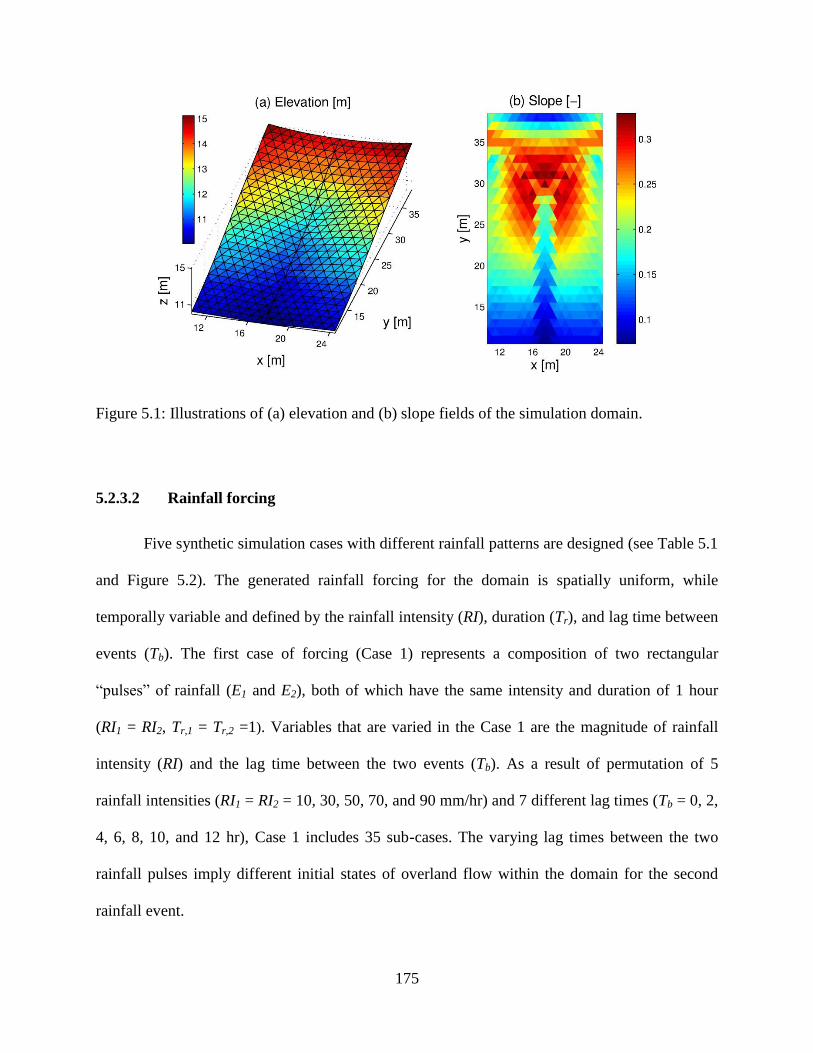
175

Figure 5.1: Illustrations of (a) elevation and (b) slope fields of the simulation domain.

5.2.3.2 Rainfall forcing

Five synthetic simulation cases with different rainfall patterns are designed (see Table 5.1

and Figure 5.2). The generated rainfall forcing for the domain is spatially uniform, while

temporally variable and defined by the rainfall intensity (RI), duration (Tr), and lag time between

events (Tb). The first case of forcing (Case 1) represents a composition of two rectangular

“pulses” of rainfall (E1 and E2), both of which have the same intensity and duration of 1 hour

(RI1 = RI2, Tr,1 = Tr,2 =1). Variables that are varied in the Case 1 are the magnitude of rainfall

intensity (RI) and the lag time between the two events (Tb). As a result of permutation of 5

rainfall intensities (RI1 = RI2 = 10, 30, 50, 70, and 90 mm/hr) and 7 different lag times (Tb = 0, 2,

4, 6, 8, 10, and 12 hr), Case 1 includes 35 sub-cases. The varying lag times between the two

rainfall pulses imply different initial states of overland flow within the domain for the second

rainfall event.

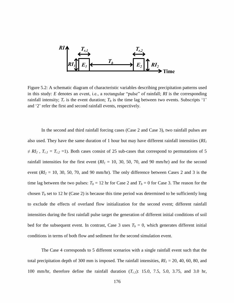
176

Figure 5.2: A schematic diagram of characteristic variables describing precipitation patterns used

in this study: E denotes an event, i.e., a rectangular “pulse” of rainfall; RI is the corresponding

rainfall intensity; Tr is the event duration; Tb is the time lag between two events. Subscripts „1‟

and „2‟ refer the first and second rainfall events, respectively.

In the second and third rainfall forcing cases (Case 2 and Case 3), two rainfall pulses are

also used. They have the same duration of 1 hour but may have different rainfall intensities (RI1

≠ RI2 , Tr,1 = Tr,2 =1). Both cases consist of 25 sub-cases that correspond to permutations of 5

rainfall intensities for the first event (RI1 = 10, 30, 50, 70, and 90 mm/hr) and for the second

event (RI2 = 10, 30, 50, 70, and 90 mm/hr). The only difference between Cases 2 and 3 is the

time lag between the two pulses: Tb = 12 hr for Case 2 and Tb = 0 for Case 3. The reason for the

chosen Tb set to 12 hr (Case 2) is because this time period was determined to be sufficiently long

to exclude the effects of overland flow initialization for the second event; different rainfall

intensities during the first rainfall pulse target the generation of different initial conditions of soil

bed for the subsequent event. In contrast, Case 3 uses Tb = 0, which generates different initial

conditions in terms of both flow and sediment for the second simulation event.

The Case 4 corresponds to 5 different scenarios with a single rainfall event such that the

total precipitation depth of 300 mm is imposed. The rainfall intensities, RI1 = 20, 40, 60, 80, and

100 mm/hr, therefore define the rainfall duration (Tr,1): 15.0, 7.5, 5.0, 3.75, and 3.0 hr,

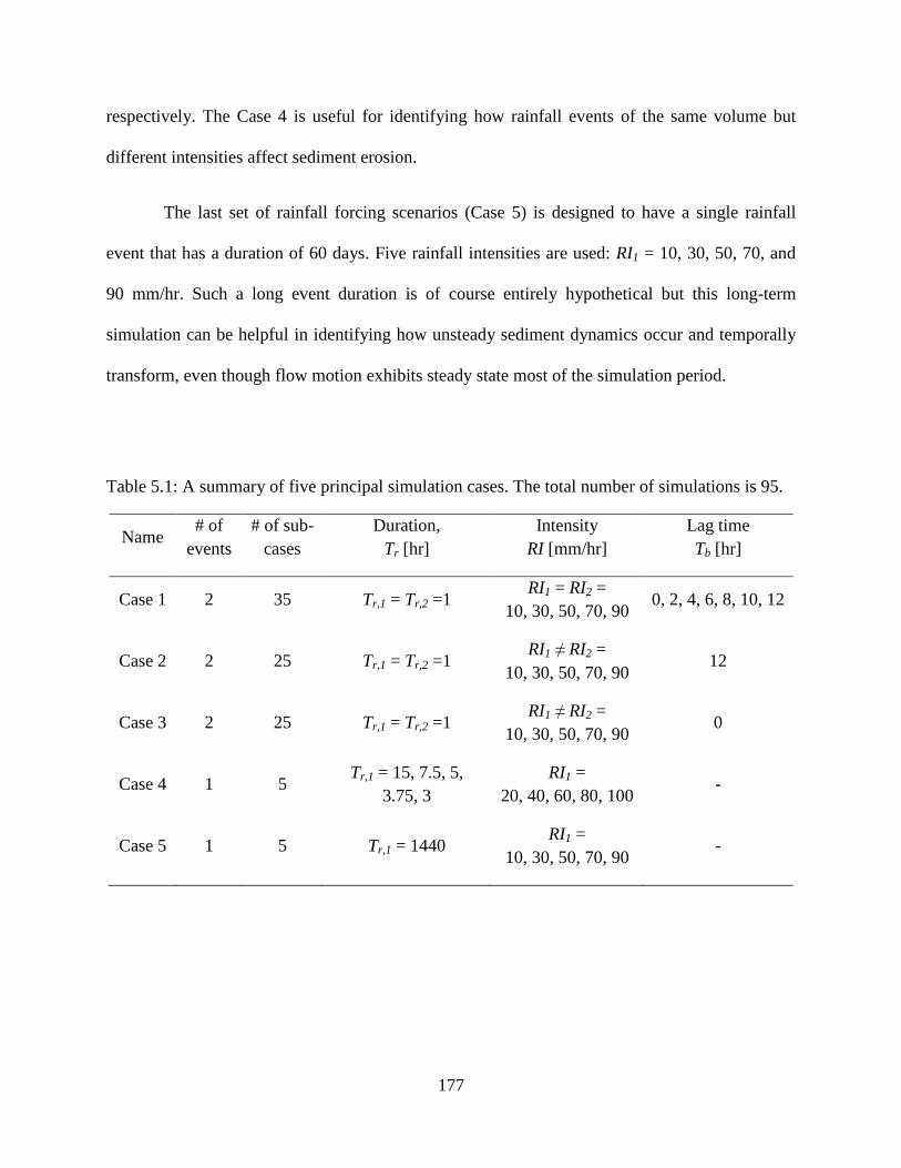
177

respectively. The Case 4 is useful for identifying how rainfall events of the same volume but

different intensities affect sediment erosion.

The last set of rainfall forcing scenarios (Case 5) is designed to have a single rainfall

event that has a duration of 60 days. Five rainfall intensities are used: RI1 = 10, 30, 50, 70, and

90 mm/hr. Such a long event duration is of course entirely hypothetical but this long-term

simulation can be helpful in identifying how unsteady sediment dynamics occur and temporally

transform, even though flow motion exhibits steady state most of the simulation period.

Table 5.1: A summary of five principal simulation cases. The total number of simulations is 95.

Name # of

events

# of sub-

cases

Duration,

Tr [hr]

Intensity

RI [mm/hr]

Lag time

Tb [hr]

Case 1 2 35 Tr,1 = Tr,2 =1 RI1 = RI2 =

10, 30, 50, 70, 90 0, 2, 4, 6, 8, 10, 12

Case 2 2 25 Tr,1 = Tr,2 =1 RI1 ≠ RI2 =

10, 30, 50, 70, 90 12

Case 3 2 25 Tr,1 = Tr,2 =1 RI1 ≠ RI2 =

10, 30, 50, 70, 90 0

Case 4 1 5 Tr,1 = 15, 7.5, 5,

3.75, 3

RI1 =

20, 40, 60, 80, 100 -

Case 5 1 5 Tr,1 = 1440 RI1 =

10, 30, 50, 70, 90 -

178

5.2.3.3 Soil characterization

In this study, silty sand soil that has four different particle fractions, each contributing an

equal fraction of 25 %, is considered as an initial bed condition for all simulation cases (i.e., at

time equal to zero). The sediment sizes of considered soil particle types are assumed to be 0.02,

0.05, 0.1, and 0.5 mm, respectively. The smallest particle type is called S1, the second smallest

and progressively larger particle types are respectively called S2, S3, and S4 types. Their

corresponding settling velocities, , are 0.000276, 0.0017, 0.0062, and 0.0619 m/s. They are

calculated using a formula of Cheng [1997].

Note that when fine-sized dry clayey soil is subjected to wetting, aggregate slaking and

breakdown will occur; conversely, crust on soil is formed when slaked soil dries. Additionally,

clay particles containing chemical elements (particularly, sodium) are prone to separate

themselves from soil aggregates in wet conditions. Since these structural (slaking) and chemical

(dispersion) mechanisms can only be implicitly incorporate in the parameters related to

erodibility, fine-sized particles are excluded from the presented numerical analysis.

An impervious soil surface condition is assumed for all simulation scenarios to exclude

the processes of infiltration and subsurface flow. While the latter certainly affects surface runoff

generation, the aim of the study is to investigate the effects of the dynamic evolution of a

shielding layer on the erosion and sediment processes in conditions of clearly identifiable

precipitation patterns. The impact of runoff-generating processes is however indirectly accounted

for through magnitudes of rainfall intensity.

179

5.2.3.4 Model parameterization

Every model that involves a description of physical phenomena faces a challenge of

parameter identification. Choosing proper values for these parameters is a necessary step before

exploratory simulations and they are usually determined either by referring to previous research

described in literature or through the process of manual/automated calibration. In this synthetic

study, the parameters summarized in Table 5.2 refer to previous research [Heng et al., 2011;

Francipane et al., 2012; Kim et al., 2013]. In the calculation of the shield effect factor by water

flow, the mean raindrop size is assumed to be 2 mm and the exponent is assumed to be 1.0 [Heng

et al., 2011]. Since the study essentially focuses on the movement of flow and sediment, the

values of landuse and soil parameters are inherited from previous studies applied for the Lucky

Hills watershed in southeastern Arizona, U.S.A. [Francipane et al., 2012; Kim et al., 2013]. The

density of sediment ( ) and water ( ) is 2,700 and 1000 kg/m3 respectively, and the porosity

of the bed is 0.46. Manning‟s coefficient of 0.03 is chosen for a representation of shear resistance.

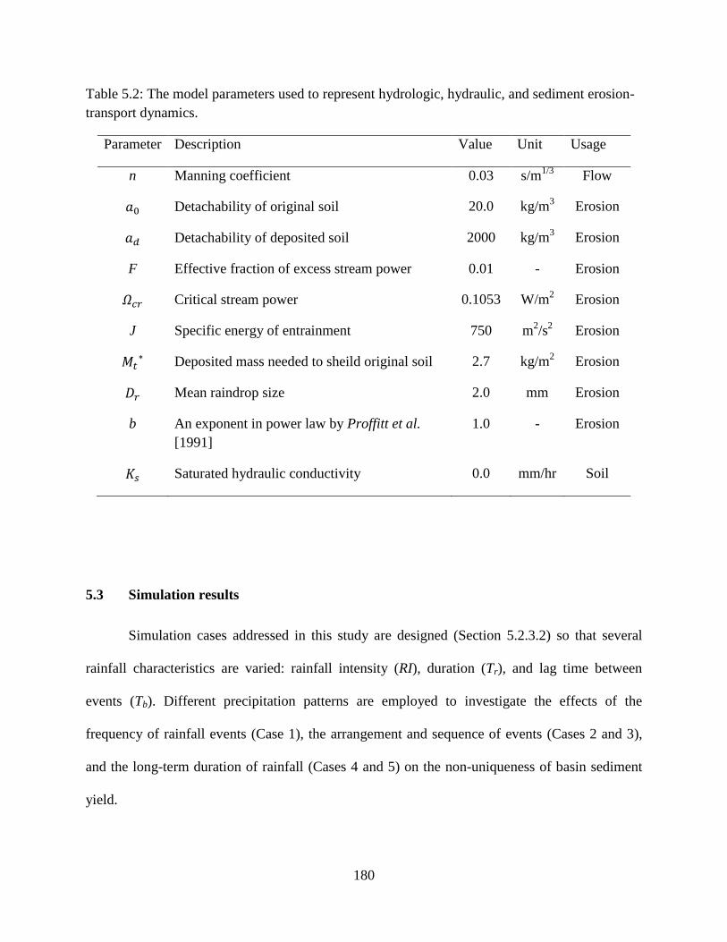
180

Table 5.2: The model parameters used to represent hydrologic, hydraulic, and sediment erosion-

transport dynamics.

Parameter Description Value Unit Usage

n Manning coefficient 0.03 s/m1/3

Flow

Detachability of original soil

20.0 kg/m3 Erosion

Detachability of deposited soil

2000 kg/m3 Erosion

F Effective fraction of excess stream power

0.01 - Erosion

Critical stream power

0.1053 W/m2 Erosion

J Specific energy of entrainment

750 m2/s

2 Erosion

Deposited mass needed to sheild original soil

2.7 kg/m

2 Erosion

Mean raindrop size 2.0 mm Erosion

b An exponent in power law by Proffitt et al.

[1991]

1.0 - Erosion

Saturated hydraulic conductivity 0.0 mm/hr Soil

5.3 Simulation results

Simulation cases addressed in this study are designed (Section 5.2.3.2) so that several

rainfall characteristics are varied: rainfall intensity (RI), duration (Tr), and lag time between

events (Tb). Different precipitation patterns are employed to investigate the effects of the

frequency of rainfall events (Case 1), the arrangement and sequence of events (Cases 2 and 3),

and the long-term duration of rainfall (Cases 4 and 5) on the non-uniqueness of basin sediment

yield.

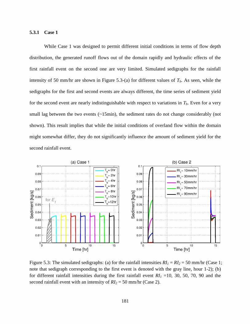
181

5.3.1 Case 1

While Case 1 was designed to permit different initial conditions in terms of flow depth

distribution, the generated runoff flows out of the domain rapidly and hydraulic effects of the

first rainfall event on the second one are very limited. Simulated sedigraphs for the rainfall

intensity of 50 mm/hr are shown in Figure 5.3-(a) for different values of Tb. As seen, while the

sedigraphs for the first and second events are always different, the time series of sediment yield

for the second event are nearly indistinguishable with respect to variations in Tb. Even for a very

small lag between the two events (~15min), the sediment rates do not change considerably (not

shown). This result implies that while the initial conditions of overland flow within the domain

might somewhat differ, they do not significantly influence the amount of sediment yield for the

second rainfall event.

Figure 5.3: The simulated sedigraphs: (a) for the rainfall intensities RI1 = RI2 = 50 mm/hr (Case 1;

note that sedigraph corresponding to the first event is denoted with the gray line, hour 1-2); (b)

for different rainfall intensities during the first rainfall event RI1 =10, 30, 50, 70, 90 and the

second rainfall event with an intensity of RI2 = 50 mm/hr (Case 2).

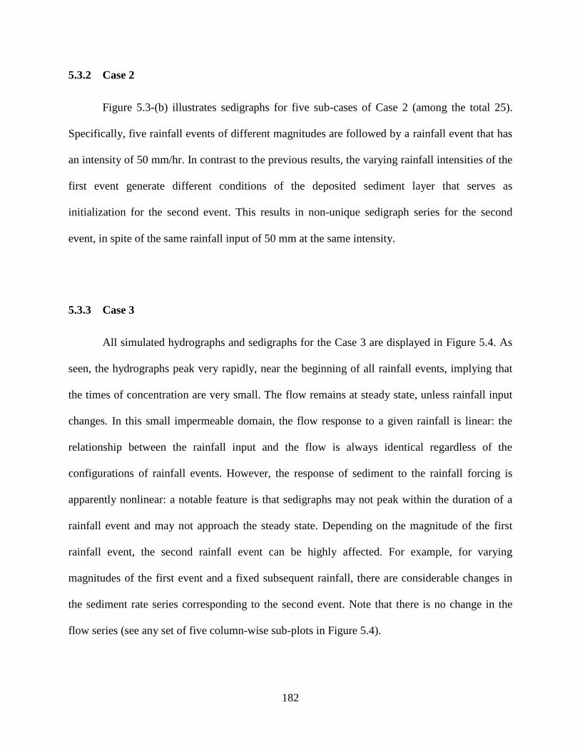
182

5.3.2 Case 2

Figure 5.3-(b) illustrates sedigraphs for five sub-cases of Case 2 (among the total 25).

Specifically, five rainfall events of different magnitudes are followed by a rainfall event that has

an intensity of 50 mm/hr. In contrast to the previous results, the varying rainfall intensities of the

first event generate different conditions of the deposited sediment layer that serves as

initialization for the second event. This results in non-unique sedigraph series for the second

event, in spite of the same rainfall input of 50 mm at the same intensity.

5.3.3 Case 3

All simulated hydrographs and sedigraphs for the Case 3 are displayed in Figure 5.4. As

seen, the hydrographs peak very rapidly, near the beginning of all rainfall events, implying that

the times of concentration are very small. The flow remains at steady state, unless rainfall input

changes. In this small impermeable domain, the flow response to a given rainfall is linear: the

relationship between the rainfall input and the flow is always identical regardless of the

configurations of rainfall events. However, the response of sediment to the rainfall forcing is

apparently nonlinear: a notable feature is that sedigraphs may not peak within the duration of a

rainfall event and may not approach the steady state. Depending on the magnitude of the first

rainfall event, the second rainfall event can be highly affected. For example, for varying

magnitudes of the first event and a fixed subsequent rainfall, there are considerable changes in

the sediment rate series corresponding to the second event. Note that there is no change in the

flow series (see any set of five column-wise sub-plots in Figure 5.4).

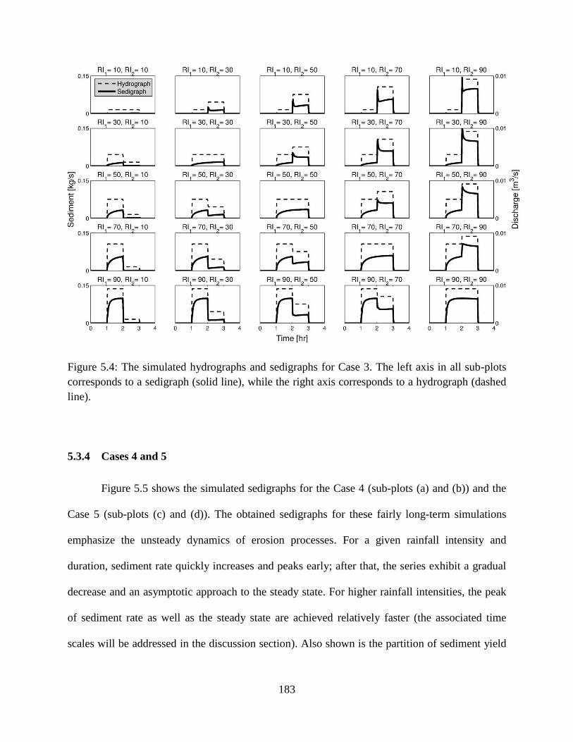
183

Figure 5.4: The simulated hydrographs and sedigraphs for Case 3. The left axis in all sub-plots

corresponds to a sedigraph (solid line), while the right axis corresponds to a hydrograph (dashed

line).

5.3.4 Cases 4 and 5

Figure 5.5 shows the simulated sedigraphs for the Case 4 (sub-plots (a) and (b)) and the

Case 5 (sub-plots (c) and (d)). The obtained sedigraphs for these fairly long-term simulations

emphasize the unsteady dynamics of erosion processes. For a given rainfall intensity and

duration, sediment rate quickly increases and peaks early; after that, the series exhibit a gradual

decrease and an asymptotic approach to the steady state. For higher rainfall intensities, the peak

of sediment rate as well as the steady state are achieved relatively faster (the associated time

scales will be addressed in the discussion section). Also shown is the partition of sediment yield

184

into absolute (Figure 5.5-(b)) or relative (Figure 5.5-(d)) fractions corresponding to the four

particle sizes (S1 through S4). The notable feature in the Case 4 is that despite the same runoff

volume, the total sediment yield for RI1 = 100 mm/hr is almost three times higher than that for

RI1 = 20 mm/hr (specifically, 431.65 vs. 1146.2 kg). Such a large difference is mainly

attributable to the high erosion loss of large-sized particles. Similarly, the results in Figure 5.5-(d)

show that higher rainfall intensities result in a progressively larger flow rate sufficient to entrain

and move larger particles, giving rise to very high nonlinearities of the total (and relative,

partitioned) sediment yields.

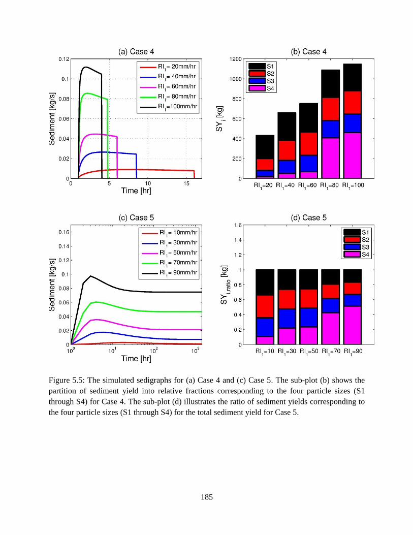
185

Figure 5.5: The simulated sedigraphs for (a) Case 4 and (c) Case 5. The sub-plot (b) shows the

partition of sediment yield into relative fractions corresponding to the four particle sizes (S1

through S4) for Case 4. The sub-plot (d) illustrates the ratio of sediment yields corresponding to

the four particle sizes (S1 through S4) for the total sediment yield for Case 5.

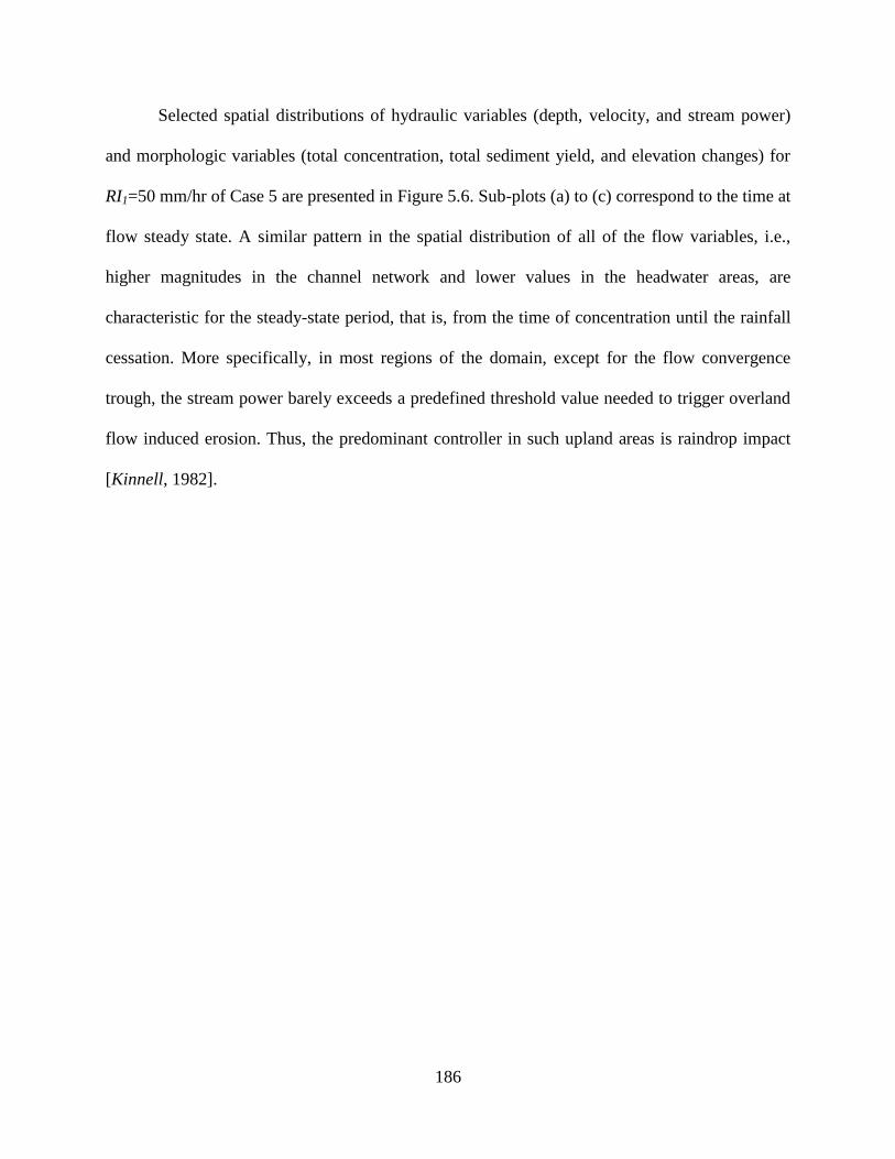
186

Selected spatial distributions of hydraulic variables (depth, velocity, and stream power)

and morphologic variables (total concentration, total sediment yield, and elevation changes) for

RI1=50 mm/hr of Case 5 are presented in Figure 5.6. Sub-plots (a) to (c) correspond to the time at

flow steady state. A similar pattern in the spatial distribution of all of the flow variables, i.e.,

higher magnitudes in the channel network and lower values in the headwater areas, are

characteristic for the steady-state period, that is, from the time of concentration until the rainfall

cessation. More specifically, in most regions of the domain, except for the flow convergence

trough, the stream power barely exceeds a predefined threshold value needed to trigger overland

flow induced erosion. Thus, the predominant controller in such upland areas is raindrop impact

[Kinnell, 1982].

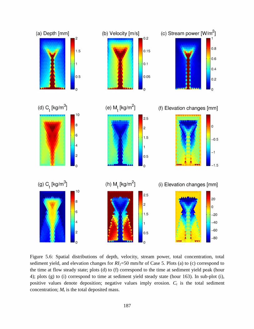
187

Figure 5.6: Spatial distributions of depth, velocity, stream power, total concentration, total

sediment yield, and elevation changes for RI1=50 mm/hr of Case 5. Plots (a) to (c) correspond to

the time at flow steady state; plots (d) to (f) correspond to the time at sediment yield peak (hour

4); plots (g) to (i) correspond to time at sediment yield steady state (hour 163). In sub-plot (i),

positive values denote deposition; negative values imply erosion. Ct is the total sediment

concentration; Mt is the total deposited mass.

188

Conversely to the temporal invariance of the flow state, the spatial pattern of

morphologic variables continuously changes until the steady-state is reached. The simulated

morphologic variables are compared for two time instants: sub-plots (d) to (f) correspond to the

peak of sediment yield, and sub-plots (g) to (i) correspond to the sediment yield steady-state

(these two critical times will be further compared in the discussion section). As seen from these

two sets of sub-plots, sediment concentrations decrease from the peak yield time to the steady

state, and they are particularly high in the area of flow convergence. In contrast, the deposited

mass temporally increases and is higher in the headwater areas due to their low stream power.

Last, the elevation changes are computed to investigate regions where the domain has eroded

(negative magnitudes) or sediment deposition has occurred (positive magnitudes). Overall,

extensive areas have eroded with especially high erosion rates in steeper regions; the amount of

erosion has consistently increased with the rainfall duration (sub-plot (f) vs. sub-plot (i)).

5.4 Discussion

5.4.1 Variations of sediment yield for the same flow volume

Several of the presented simulation results vividly demonstrate that there can be a

considerable variation in sediment yield despite the same rainfall volume. While the dependence

on rainfall rate has been long discussed in literature [Edwards and Owens, 1991; Romkens et al.,

2001; Abu Hammad et al., 2006; Ahmadi et al., 2010; Svoray and Ben-Said, 2010], the results of

this study address the importance of additional mechanisms that can cause similar conditions of

non-uniqueness. Figure 5.7 summarizes the addressed variability by displaying event runoff

volume versus the corresponding sediment yield for all of the considered Cases. The initial

189

condition of soil bed at the simulation start is “intact”, i.e., the soil has not yet been disturbed.

This results in a low erodibility of the soil bed, leading to relatively low erosion. This is opposite

to the effect of a looser soil condition at the onset of subsequent rainfall event (Cases 1-3, 5).

Thus, the sediment yields for two events can be different, while corresponding to the same flow

volume (Figure 5.7-(a), (b), and (c)).

Using the above inference (and results shown in Figure 5.7-(a) to (c)), the eroded material

generated during the first hour should be progressively smaller than sediment flux leaving the

basin during later hours. However, a notable result in Figure 5.7-(f) is that SY corresponding to

later hours can be smaller than that for the first hour. This result is of interest because in

conditions of a relatively loose soil bed material, the erosion loss can become smaller than that

for soil in initial, intact condition exhibiting low detachability. Such an outcome indicates that

there exists a mechanism that hampers progressively higher erosion. This study argues that the

mechanism is mainly attributed to the development of a shielding layer that protects underlying

soil, counteracting the effect of an increasing amount of loose material.

190

Figure 5.7: Flow volume (FV) versus sediment yield (SY) for all simulation cases. FV and SY are

computed by integrating the flow and the sediment rates of the corresponding hydrographs and

sedigraphs. The red squares correspond to the first rainfall event (1 hour duration, Cases 1, 2, and

3) or simply the first simulation hour (Case 5), for which the initial condition of soil bed was not

„disturbed‟ (i.e., intact soil bed condition). Black stars correspond to either the second event

(Cases 1, 2, and 3 in sub-plots (a)-(c)), the entire single event (Cases 3 and 4, sub-plots (d)-(e)),

or hourly volumes (Case 5, sub-plot (f)). Specifically, sub-plots (d) and (e) illustrate FVt and SYt

that were computed for the entire simulation period of Cases 3 and 4 to ensure the same runoff

volume. Sub-plot (f) illustrates a regression between hourly sediment yield (SYhr) and flow (FVhr)

of Case 5.

191

For all of the simulated Cases, a statistical metric is introduced to illustrate how a given

precipitation scenario affects the variation of eroded sediment mass. Given the same rainfall

volume, the variation of sediment yield mass VSY (in percent) is defined as

where the subscripts “max” and “min” refer to maximum and minimum values among sediment

yields (depicted as black stars in Figure 5.7, i.e., excluding the red squares) for the same flow

volume. Table 5.3 shows the computed values of VSY for all Cases shown in Figure 5.7.

According to these estimates, the range of non-uniqueness caused by the effects of time lag

between two successive events of the same magnitude is extremely small (less than 3 %, Case 1).

Conversely, sediment dynamics, as affected by magnitude of a previous rainfall event, can result

in SY variations ranging from 7.88 to 26.6 % (Cases 2 and 3). Even larger variations in the total

or hourly SY can occur in Cases 4 and 5, implying that longer intervals of coupled flow-sediment

dynamics are likely to exhibit a more pronounced non-unique behavior in response to the same

input.

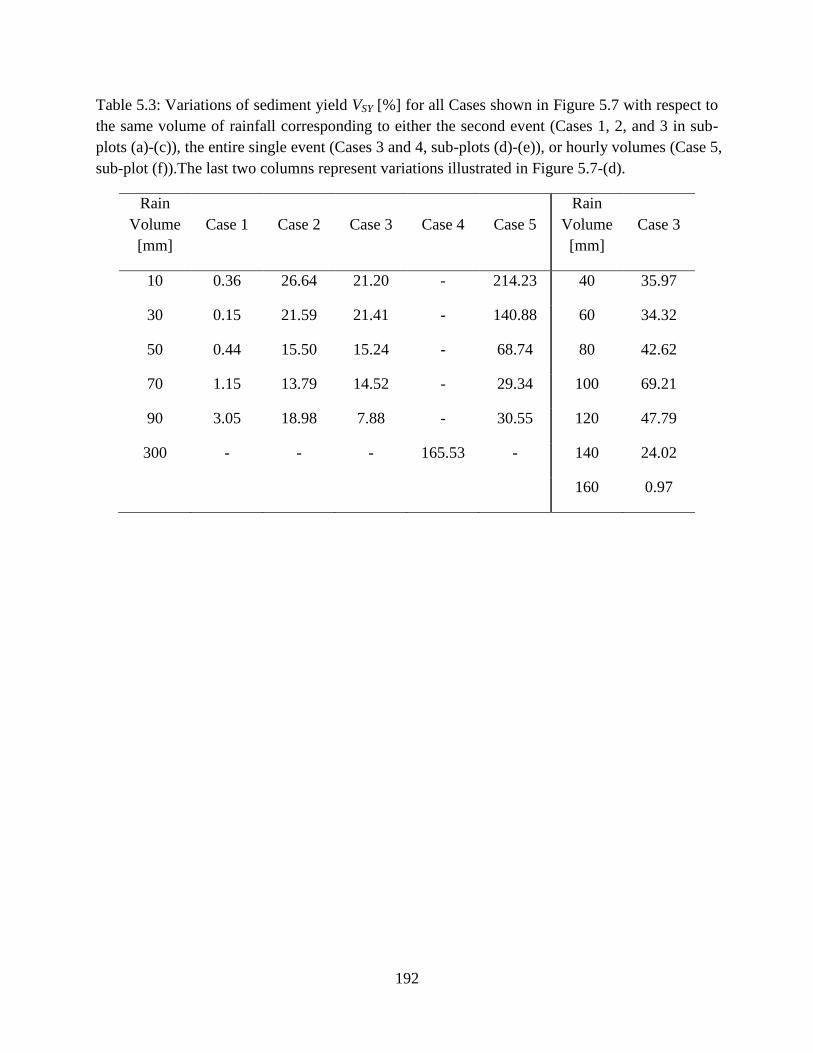
192

Table 5.3: Variations of sediment yield VSY [%] for all Cases shown in Figure 5.7 with respect to

the same volume of rainfall corresponding to either the second event (Cases 1, 2, and 3 in sub-

plots (a)-(c)), the entire single event (Cases 3 and 4, sub-plots (d)-(e)), or hourly volumes (Case 5,

sub-plot (f)).The last two columns represent variations illustrated in Figure 5.7-(d).

Rain

Volume

[mm]

Case 1 Case 2

Case 3

Case 4 Case 5

Rain

Volume

[mm]

Case 3

10 0.36 26.64 21.20 - 214.23 40 35.97

30 0.15 21.59 21.41 - 140.88 60 34.32

50 0.44 15.50 15.24 - 68.74 80 42.62

70 1.15 13.79 14.52 - 29.34 100 69.21

90 3.05 18.98 7.88 - 30.55 120 47.79

300 - - - 165.53 - 140 24.02

160 0.97

193

The last two columns of Table 5.3 illustrate the erosion response based on estimates in

Figure 5.7-(d), which show the total sediment yields associated with two-hour rainfall periods;

SY variations were subsequently computed for the same rainfall volume (Case 3). Additionally, if

one separately examines sequences of either increasing or decreasing rainfall magnitude in Case

3, the total SY corresponding to the sequence with an increasing trend is always greater than that

for a sequence of events with decreasing magnitude. The corresponding variability of the total

yield for the same rainfall volume was computed by comparing ten sub-case sets with both

increasing and decreasing trends (e.g., one of the sets consists of two sub-cases, i.e., RI1 = 10, RI2

= 30 and RI1 = 30, RI2 = 10 mm/hr, etc.), which resulted in the range from 1.0 to 36 % (not

shown). This variability indicates that depending on whether a storm interval with a higher

erosive power occurs at the beginning or the end and depending on how significantly soil bed is

perturbed during or prior to it, the prediction of the total sediment loss is strongly affected. In the

context of the considered scenario of a continuous 2-hour storm (Case 3), a higher rainfall during

the second hour (applied in conditions of soil that was perturbed by the rainfall of the first hour)

implies a larger erosion capacity. A similar conclusion was obtained experimentally by Romkens

et al. [2001] for the case of 2% slope. However, an opposite result was obtained for the other two

slopes used by Romkens et al. [2001]: a decreasing precipitation rate yielded a larger sediment

loss. This was primarily attributed to the surface rilling, which was more severe for a decreasing

storm rate, and to the surface sealing, which is unlikely to occur for an initial rainfall of a higher

intensity. Although the numerical model used here does not consider the processes of sealing or

rill formation, another considerable issue associated with this disparity is in the fact that the

study of Romkens et al. [2001] did not use particles of larger sizes, being only constrained to 98%

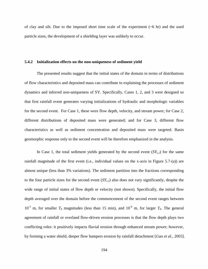
194

of clay and silt. Due to the imposed short time scale of the experiment (~6 hr) and the used

particle sizes, the development of a shielding layer was unlikely to occur.

5.4.2 Initialization effects on the non-uniqueness of sediment yield

The presented results suggest that the initial states of the domain in terms of distributions

of flow characteristics and deposited mass can contribute to explaining the processes of sediment

dynamics and inferred non-uniqueness of SY. Specifically, Cases 1, 2, and 3 were designed so

that first rainfall event generates varying initializations of hydraulic and morphologic variables

for the second event. For Case 1, these were flow depth, velocity, and stream power; for Case 2,

different distributions of deposited mass were generated; and for Case 3, different flow

characteristics as well as sediment concentration and deposited mass were targeted. Basin

geomorphic response only to the second event will be therefore emphasized in the analysis.

In Case 1, the total sediment yields generated by the second event (SYt,2) for the same

rainfall magnitude of the first event (i.e., individual values on the x-axis in Figure 5.7-(a)) are

almost unique (less than 3% variations). The sediment partition into the fractions corresponding

to the four particle sizes for the second event (SYi,2) also does not vary significantly, despite the

wide range of initial states of flow depth or velocity (not shown). Specifically, the initial flow

depth averaged over the domain before the commencement of the second event ranges between

10-3

m, for smaller Tb magnitudes (less than 15 min), and 10-6

m, for larger Tb. The general

agreement of rainfall or overland flow-driven erosion processes is that the flow depth plays two

conflicting roles: it positively impacts fluvial erosion through enhanced stream power; however,

by forming a water shield, deeper flow hampers erosion by rainfall detachment [Gao et al., 2003].

195

The obtained outcome of Case 1 is because the effects of depth are very minor: the domain is of

zero-order and therefore there is no sufficient flow accumulation. While the domain conditions

represent an idealized simulation case, the same phenomenon can be expected in headwater areas

of complex topography exhibiting a small fraction of surface runoff detention.

In Cases 2 and 3, different spatial compositions of bed in terms of original, „intact‟ soil

and non-local sediment material transported and deposited locally prior to the second event were

obtained. In order to capture the differences between the corresponding composition states,

particle size distributions of the deposited mass prior to the second event (Mi,2ini

) are averaged

spatially and presented in Figure 5.8 (for RI2=50 mm/hr only). Higher magnitudes of Mi,2ini

represent a larger proportion of the deposited, loose material. Depending on preceding rainfall

(i.e., the magnitude of RI1), the local surface condition of soil can be partially altered; 5 (smallest

rainfall rate) to 20 % (highest rainfall rate) of intact soil was changed to the deposited soil. The

deposited sediment also exhibits spatially varying PSDs, which can be very different from the

uniform distribution of sizes in the original, intact soil. As seen in Figure 5.8-(b) and (d), a

smaller rainfall intensity of the first event leads to a PSD similar to that of the original soil.

Conversely, larger magnitudes of the first event transform the composition of the surface soil

dramatically, which can become composed of predominantly coarser particles (see Figure 5.8-(b)

and (d)). It can be also inferred that as Mi,2ini

increases, sediment yield (SYi,2) also grows initially

because the deposited soil material has higher erodibility, as compared to the original soil.

However, SYi,2 exhibits a maximum at lower magnitudes of the deposited soil material and shows

a decay for larger Mi,2ini

(for both Cases 2 and 3, Figure 5.8-(a) and (c)). A similar pattern of

dependence is obtained for other magnitudes of RI2 (not shown). Such a peculiar behavior is

explained by the growing fraction of coarser particles that have high settling velocities: through

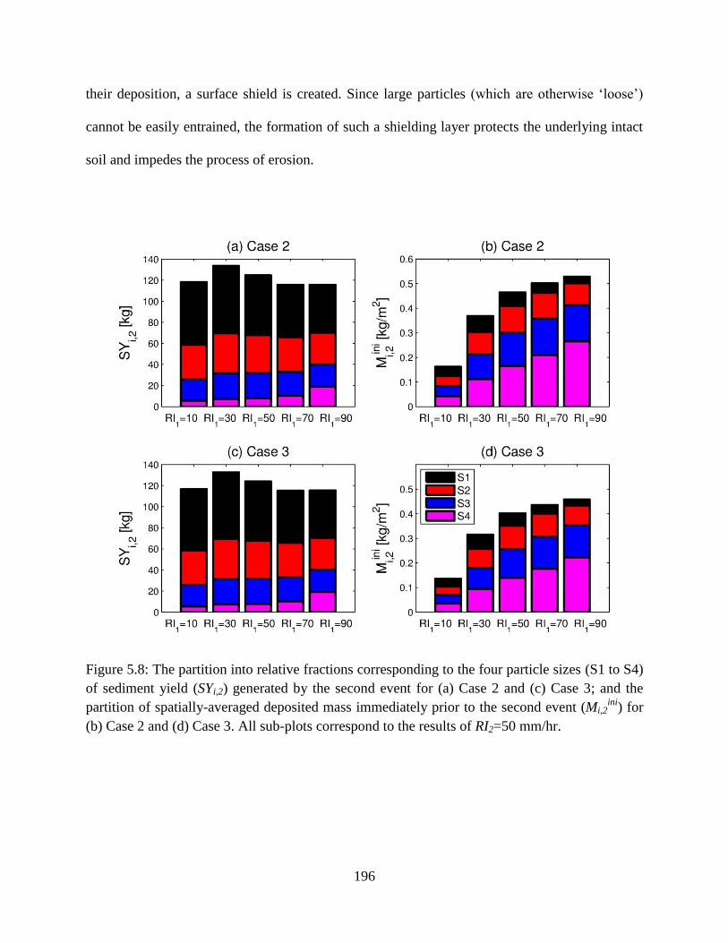
196

their deposition, a surface shield is created. Since large particles (which are otherwise „loose‟)

cannot be easily entrained, the formation of such a shielding layer protects the underlying intact

soil and impedes the process of erosion.

Figure 5.8: The partition into relative fractions corresponding to the four particle sizes (S1 to S4)

of sediment yield (SYi,2) generated by the second event for (a) Case 2 and (c) Case 3; and the

partition of spatially-averaged deposited mass immediately prior to the second event (Mi,2ini

) for

(b) Case 2 and (d) Case 3. All sub-plots correspond to the results of RI2=50 mm/hr.

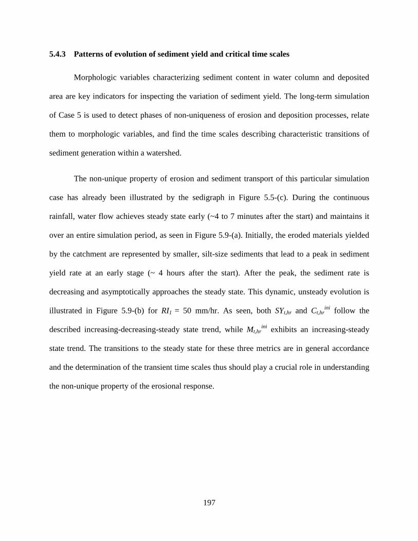
197

5.4.3 Patterns of evolution of sediment yield and critical time scales

Morphologic variables characterizing sediment content in water column and deposited

area are key indicators for inspecting the variation of sediment yield. The long-term simulation

of Case 5 is used to detect phases of non-uniqueness of erosion and deposition processes, relate

them to morphologic variables, and find the time scales describing characteristic transitions of

sediment generation within a watershed.

The non-unique property of erosion and sediment transport of this particular simulation

case has already been illustrated by the sedigraph in Figure 5.5-(c). During the continuous

rainfall, water flow achieves steady state early (~4 to 7 minutes after the start) and maintains it

over an entire simulation period, as seen in Figure 5.9-(a). Initially, the eroded materials yielded

by the catchment are represented by smaller, silt-size sediments that lead to a peak in sediment

yield rate at an early stage (~ 4 hours after the start). After the peak, the sediment rate is

decreasing and asymptotically approaches the steady state. This dynamic, unsteady evolution is

illustrated in Figure 5.9-(b) for RI1 = 50 mm/hr. As seen, both SYt,hr and Ct,hrini

follow the

described increasing-decreasing-steady state trend, while Mt,hrini

exhibits an increasing-steady

state trend. The transitions to the steady state for these three metrics are in general accordance

and the determination of the transient time scales thus should play a crucial role in understanding

the non-unique property of the erosional response.

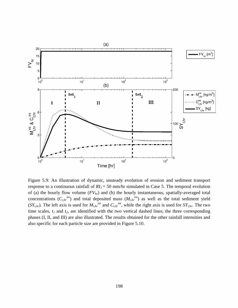
198

Figure 5.9: An illustration of dynamic, unsteady evolution of erosion and sediment transport

response to a continuous rainfall of RI1 = 50 mm/hr simulated in Case 5. The temporal evolution

of (a) the hourly flow volume (FVhr) and (b) the hourly instantaneous, spatially-averaged total

concentrations (Ct,hrini

) and total deposited mass (Mt,hrini

) as well as the total sediment yield

(SYt,hr). The left axis is used for Mt,hrini

and Ct,hrini

, while the right axis is used for SYt,hr. The two

time scales, t1 and t2, are identified with the two vertical dashed lines; the three corresponding

phases (I, II, and III) are also illustrated. The results obtained for the other rainfall intensities and

also specific for each particle size are provided in Figure 5.10.

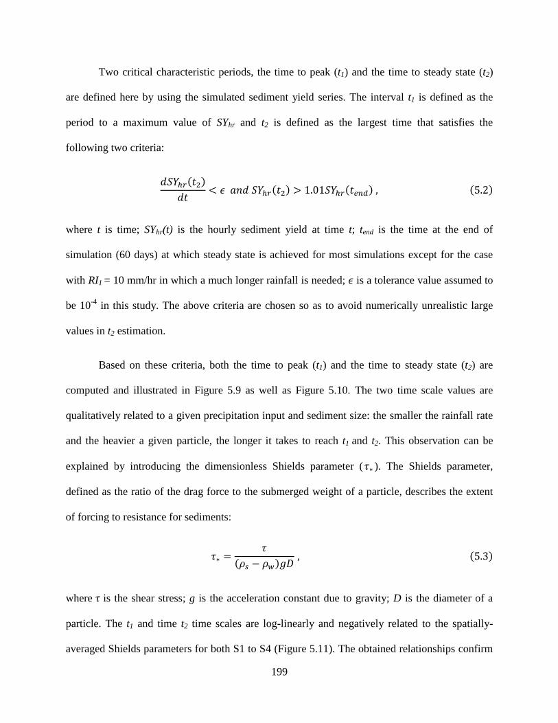
199

Two critical characteristic periods, the time to peak (t1) and the time to steady state (t2)

are defined here by using the simulated sediment yield series. The interval t1 is defined as the

period to a maximum value of SYhr and t2 is defined as the largest time that satisfies the

following two criteria:

where t is time; SYhr(t) is the hourly sediment yield at time t; tend is the time at the end of

simulation (60 days) at which steady state is achieved for most simulations except for the case

with RI1 = 10 mm/hr in which a much longer rainfall is needed; is a tolerance value assumed to

be 10-4

in this study. The above criteria are chosen so as to avoid numerically unrealistic large

values in t2 estimation.

Based on these criteria, both the time to peak (t1) and the time to steady state (t2) are

computed and illustrated in Figure 5.9 as well as Figure 5.10. The two time scale values are

qualitatively related to a given precipitation input and sediment size: the smaller the rainfall rate

and the heavier a given particle, the longer it takes to reach t1 and t2. This observation can be

explained by introducing the dimensionless Shields parameter ( ). The Shields parameter,

defined as the ratio of the drag force to the submerged weight of a particle, describes the extent

of forcing to resistance for sediments:

where is the shear stress; g is the acceleration constant due to gravity; D is the diameter of a

particle. The t1 and time t2 time scales are log-linearly and negatively related to the spatially-

averaged Shields parameters for both S1 to S4 (Figure 5.11). The obtained relationships confirm

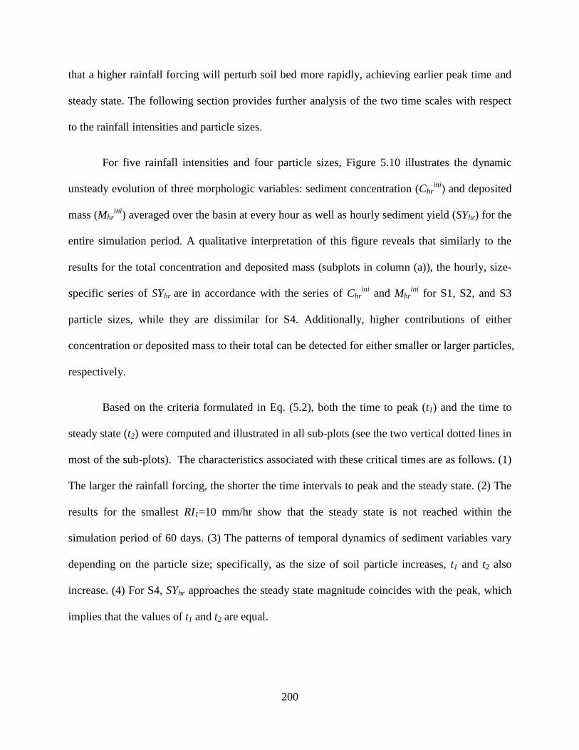
200

that a higher rainfall forcing will perturb soil bed more rapidly, achieving earlier peak time and

steady state. The following section provides further analysis of the two time scales with respect

to the rainfall intensities and particle sizes.

For five rainfall intensities and four particle sizes, Figure 5.10 illustrates the dynamic

unsteady evolution of three morphologic variables: sediment concentration (Chrini

) and deposited

mass (Mhrini

) averaged over the basin at every hour as well as hourly sediment yield (SYhr) for the

entire simulation period. A qualitative interpretation of this figure reveals that similarly to the

results for the total concentration and deposited mass (subplots in column (a)), the hourly, size-

specific series of SYhr are in accordance with the series of Chrini

and Mhrini

for S1, S2, and S3

particle sizes, while they are dissimilar for S4. Additionally, higher contributions of either

concentration or deposited mass to their total can be detected for either smaller or larger particles,

respectively.

Based on the criteria formulated in Eq. (5.2), both the time to peak (t1) and the time to

steady state (t2) were computed and illustrated in all sub-plots (see the two vertical dotted lines in

most of the sub-plots). The characteristics associated with these critical times are as follows. (1)

The larger the rainfall forcing, the shorter the time intervals to peak and the steady state. (2) The

results for the smallest RI1=10 mm/hr show that the steady state is not reached within the

simulation period of 60 days. (3) The patterns of temporal dynamics of sediment variables vary

depending on the particle size; specifically, as the size of soil particle increases, t1 and t2 also

increase. (4) For S4, SYhr approaches the steady state magnitude coincides with the peak, which

implies that the values of t1 and t2 are equal.

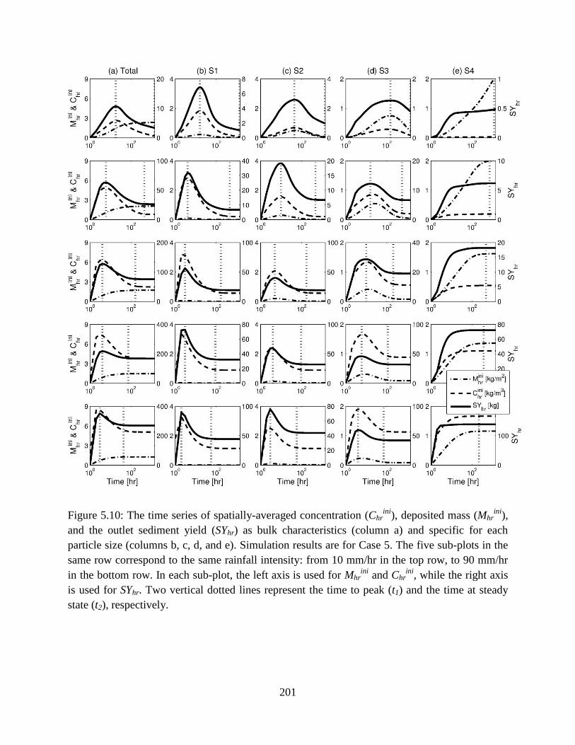
201

Figure 5.10: The time series of spatially-averaged concentration (Chrini

), deposited mass (Mhrini

),

and the outlet sediment yield (SYhr) as bulk characteristics (column a) and specific for each

particle size (columns b, c, d, and e). Simulation results are for Case 5. The five sub-plots in the

same row correspond to the same rainfall intensity: from 10 mm/hr in the top row, to 90 mm/hr

in the bottom row. In each sub-plot, the left axis is used for Mhrini

and Chrini

, while the right axis

is used for SYhr. Two vertical dotted lines represent the time to peak (t1) and the time at steady

state (t2), respectively.

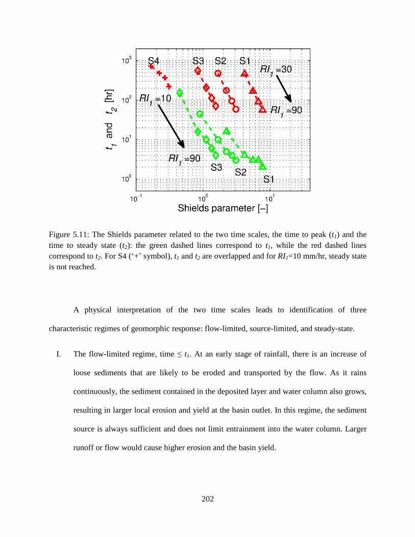
202

Figure 5.11: The Shields parameter related to the two time scales, the time to peak (t1) and the

time to steady state (t2): the green dashed lines correspond to t1, while the red dashed lines

correspond to t2. For S4 („+‟ symbol), t1 and t2 are overlapped and for RI1=10 mm/hr, steady state

is not reached.

A physical interpretation of the two time scales leads to identification of three

characteristic regimes of geomorphic response: flow-limited, source-limited, and steady-state.

I. The flow-limited regime, time ≤ t1. At an early stage of rainfall, there is an increase of

loose sediments that are likely to be eroded and transported by the flow. As it rains

continuously, the sediment contained in the deposited layer and water column also grows,

resulting in larger local erosion and yield at the basin outlet. In this regime, the sediment

source is always sufficient and does not limit entrainment into the water column. Larger

runoff or flow would cause higher erosion and the basin yield.

203

II. The source-limited regime, t1 < time ≤ t2. Continuing rain keeps driving the processes of

detachment, entrainment, and deposition, but the geomorphic response changes. Even

though the total deposited mass is continuously increasing, the basin sediment yield no

longer grows after t1. This is because of the dynamic evolution of a shielding layer

formed by larger, heavier particles. The yield of smaller-sized particles that can be easily

eroded and transported is becoming constrained by their availability across the domain,

as these particles had been mostly flushed out of the basin prior to the occurrence of t1.

The yield therefore would not respond positively to an increase in runoff/flow depth.

III. The steady-state regime, time > t2. The ratio between sediment originating from the

initially „intact‟ soil and deposited mass as well as the partition of each particle size

within the deposited soil become time-invariant, reflecting „stabilization‟ of the soil bed.

For any subsequent hours of the same rainfall forcing, the unit response will be identical.

An increase in the rainfall forcing will however drive an unsteady regime that will cause

the occurrence of all three phases of sediment dynamics, albeit with different

characteristic time scales.

5.4.4 Patterns of temporal evolution specific to particle sizes

Figure 5.12 is intended to facilitate understanding of the temporal evolution of the

spatially-averaged concentration of individual particle size Ci,hrini

and deposited mass Mi,hrini

(the

subscript „i‟ denoting the four particle sizes, S1 to S4). The occurrence of the three characteristic

regimes for these variables is also illustrated. The cumulative SYhr are shown with respect to

Ci,hrini

and deposited mass Mi,hrini

. Overall, the evolution patterns of Ci,hrini

and Mi,hrini

are

contrasting: as a particle size increases, smaller concentrations and higher deposited masses are

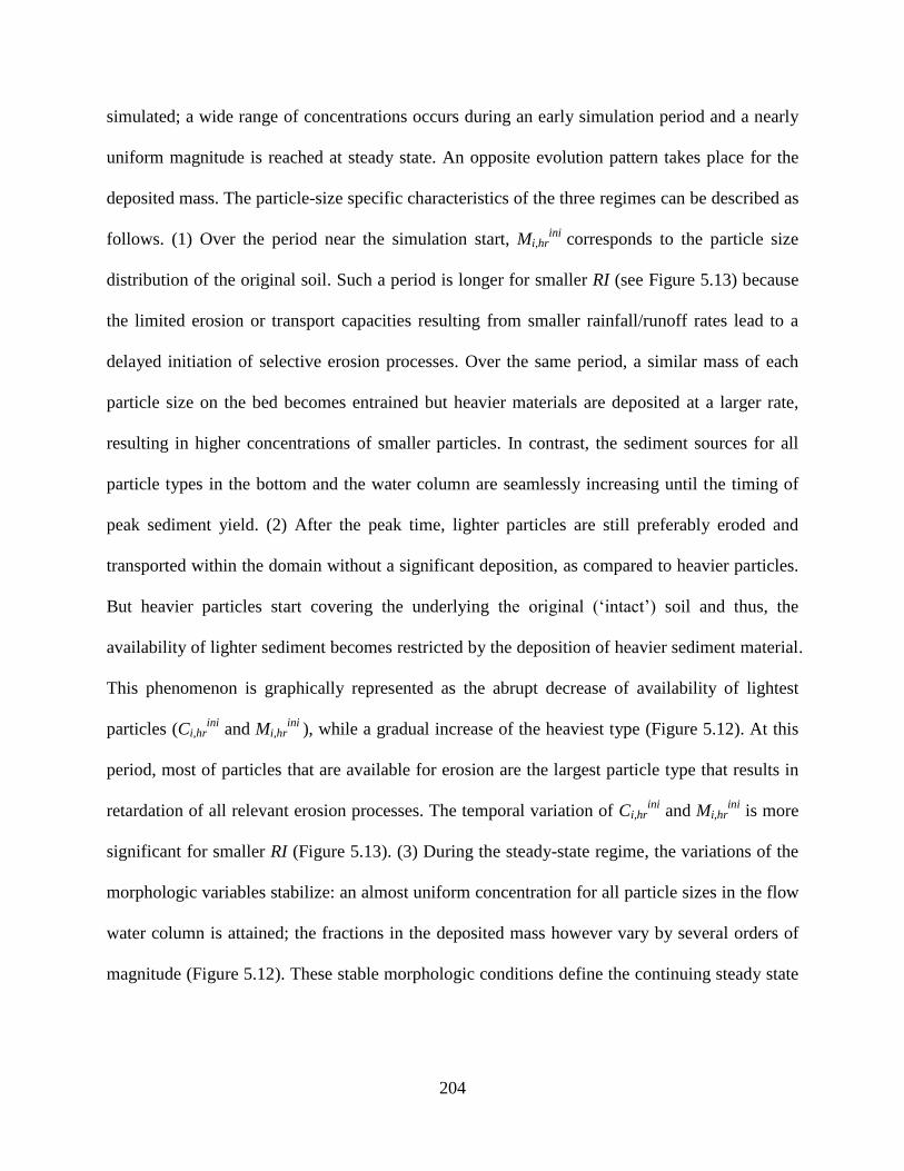
204

simulated; a wide range of concentrations occurs during an early simulation period and a nearly

uniform magnitude is reached at steady state. An opposite evolution pattern takes place for the

deposited mass. The particle-size specific characteristics of the three regimes can be described as

follows. (1) Over the period near the simulation start, Mi,hrini

corresponds to the particle size

distribution of the original soil. Such a period is longer for smaller RI (see Figure 5.13) because

the limited erosion or transport capacities resulting from smaller rainfall/runoff rates lead to a

delayed initiation of selective erosion processes. Over the same period, a similar mass of each

particle size on the bed becomes entrained but heavier materials are deposited at a larger rate,

resulting in higher concentrations of smaller particles. In contrast, the sediment sources for all

particle types in the bottom and the water column are seamlessly increasing until the timing of

peak sediment yield. (2) After the peak time, lighter particles are still preferably eroded and

transported within the domain without a significant deposition, as compared to heavier particles.

But heavier particles start covering the underlying the original („intact‟) soil and thus, the

availability of lighter sediment becomes restricted by the deposition of heavier sediment material.

This phenomenon is graphically represented as the abrupt decrease of availability of lightest

particles (Ci,hrini

and Mi,hrini

), while a gradual increase of the heaviest type (Figure 5.12). At this

period, most of particles that are available for erosion are the largest particle type that results in

retardation of all relevant erosion processes. The temporal variation of Ci,hrini

and Mi,hrini

is more

significant for smaller RI (Figure 5.13). (3) During the steady-state regime, the variations of the

morphologic variables stabilize: an almost uniform concentration for all particle sizes in the flow

water column is attained; the fractions in the deposited mass however vary by several orders of

magnitude (Figure 5.12). These stable morphologic conditions define the continuing steady state

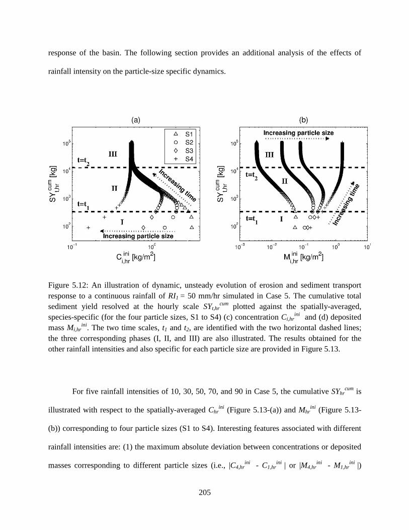
205

response of the basin. The following section provides an additional analysis of the effects of

rainfall intensity on the particle-size specific dynamics.

Figure 5.12: An illustration of dynamic, unsteady evolution of erosion and sediment transport

response to a continuous rainfall of RI1 = 50 mm/hr simulated in Case 5. The cumulative total

sediment yield resolved at the hourly scale SYt,hrcum

plotted against the spatially-averaged,

species-specific (for the four particle sizes, S1 to S4) (c) concentration Ci,hrini

and (d) deposited

mass Mi,hrini

. The two time scales, t1 and t2, are identified with the two horizontal dashed lines;

the three corresponding phases (I, II, and III) are also illustrated. The results obtained for the

other rainfall intensities and also specific for each particle size are provided in Figure 5.13.

For five rainfall intensities of 10, 30, 50, 70, and 90 in Case 5, the cumulative SYhrcum

is

illustrated with respect to the spatially-averaged Chrini

(Figure 5.13-(a)) and Mhrini

(Figure 5.13-

(b)) corresponding to four particle sizes (S1 to S4). Interesting features associated with different

rainfall intensities are: (1) the maximum absolute deviation between concentrations or deposited

masses corresponding to different particle sizes (i.e., |C4,hrini

- C1,hrini

| or |M4,hrini

- M1,hrini

|)

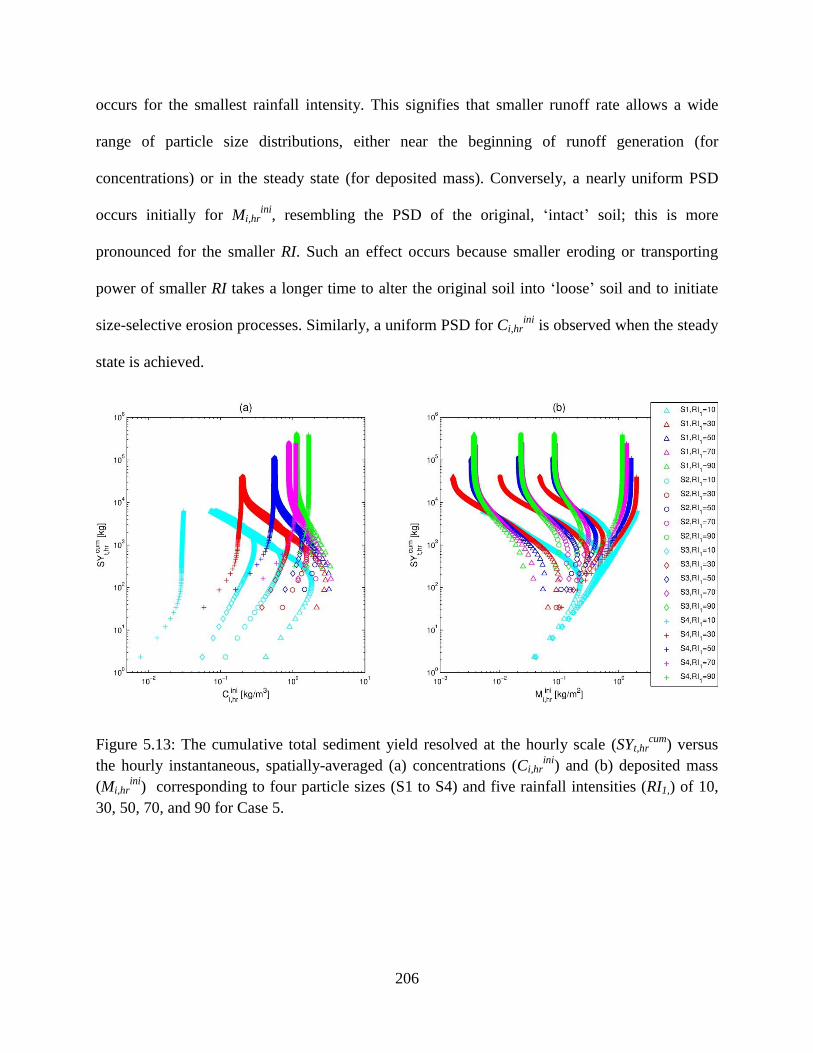
206

occurs for the smallest rainfall intensity. This signifies that smaller runoff rate allows a wide

range of particle size distributions, either near the beginning of runoff generation (for

concentrations) or in the steady state (for deposited mass). Conversely, a nearly uniform PSD

occurs initially for Mi,hrini

, resembling the PSD of the original, „intact‟ soil; this is more

pronounced for the smaller RI. Such an effect occurs because smaller eroding or transporting

power of smaller RI takes a longer time to alter the original soil into „loose‟ soil and to initiate

size-selective erosion processes. Similarly, a uniform PSD for Ci,hrini

is observed when the steady

state is achieved.

Figure 5.13: The cumulative total sediment yield resolved at the hourly scale (SYt,hrcum

) versus

the hourly instantaneous, spatially-averaged (a) concentrations (Ci,hrini

) and (b) deposited mass

(Mi,hrini

) corresponding to four particle sizes (S1 to S4) and five rainfall intensities (RI1,) of 10,

30, 50, 70, and 90 for Case 5.

207

5.5 Conclusions

This study develops a series of modeling scenarios for a zeroth-order watershed to

generate an ensemble of runoff and sediment responses simulated in a controlled fashion, i.e.,

without an explicit representation of the processes of infiltration and subsurface moisture

dynamics. The series of simulation cases are designed so that rainfall intensity, duration, and lag

time between successive events are varied. The anticipated outcome of such a design is that a

„perturbation‟ of soil substrate by an initial rainfall event influences the conditions of flow and

sediment prior to the onset of a subsequent rainfall event. Specifically, in Cases 1, 2, and 3, the

first rainfall event generates varying initializations of hydraulic and morphologic variables. For

Case 1, these are flow depth, velocity, and stream power; for Case 2, different distributions of

deposited mass are generated; and for Case 3, different flow characteristics as well as sediment

concentration and deposited mass are produced. Cases 4 and 5 represent simulations of response

to relatively long-term precipitation to resolve continuously varying morphologic bed conditions

for a steady-stated hydraulic flow regime.

The generated different initial conditions change the particle size distribution of the soil

substrate, which may form a shielding layer composed of larger particles. One of the outcomes is

that unless the initial condition of flow and sediment is identical, the same volume of runoff

(produced at the same rate) can generate different total sediment yields. For example, the

variation of sediment yield in Case 1 is nearly zero (less than 3 %), because of the limited change

in the initial condition. Conversely, the variations exhibited by the rest of the simulation cases

reach up to ~200%. In Case 3, the sediment yield is greater for a sequence of rainfall events with

increasing magnitudes, as compared to decreasing magnitudes. This is in contrast to a subset of

results by Romkens et al. [2001], which can be attributed to their smaller experimental domain

208

and soil type dominated by finer fractions (98% of clay and silt) as well as an insufficient

monitoring period (~6 hr) to observe the development of a shielding layer.

The shield formation by relatively larger particles can be one of the significant controllers

of erosion and net sediment transport at the event scale; the cycle of shield formation and

destruction is likely to be a strong contributor to the non-uniqueness of erosion dependence on

runoff. The temporal development of the shielding layer determines the amount of sediments in

the flow water column and areas of deposition, resulting in the dynamic, unsteady variation of

sediment yield. For a long-term simulation with continuous rainfall, the peculiar feature of

sediment yield is the existence of maximum before steady-state of yield is reached. The two

identified time scales, i.e., the time to peak (t1) and the time to steady-state (t2) distinguish the

corresponding transitions that help addressing the non-uniqueness property of sediment yield

from a physical standpoint. Specifically, the time scales imply the existence of three

characteristic periods which correspond to flow-limited, source-limited, and steady-state regimes.

The flow-limited regime occurs during early stages of rainfall. Continuous forcing leads to an

increase of watershed areas where sediment is detached from the soil surface by rainfall or

entrained by the flow, resulting in a net increase of erosion. In this regime, the sediment source is

sufficient and thus a larger forcing would lead to higher erosion. The source-limited regime

corresponds to the time period between t1 and t2. During this time, the total deposited mass that

has higher erodibility than the original, „intact‟ soil is continuously increasing but the domain

sediment yield diminishes after t1. This occurs because of the dynamic evolution of a shielding

layer formed by larger particles – they cause a concurrent reduction of availability of lighter

sediment because heavier particles cover the underlying intact soil. During the steady-state after

t2, soil bed conditions, i.e., the ratio of the amount of intact and loose materials, and the

209

component substrates inside the deposited area become stabilized and time-invariant. The

stabilized initial condition always provides the identical response to the same forcing. Therefore,

a unique relationship between rainfall forcing and generated sediment yield is attained at this

phase.

Soil erosion and sediment transport are complex phenomena and it has been practically

impossible to fully incorporate all relevant details in numerical models. This study addressed

only those erosion processes that are perceived to be essential: rainfall-induced detachment and

overland flow-induced entrainment of soil particles, their deposition due to gravity, and shield

effects by both larger particles and flow depth. These processes are simultaneously computed

responding to a detailed representation of flow motion. Other related processes depending on a

degree of soil saturation, slaking, dispersion, crusting, and rill formation are not taken into

account because of the intricacies of relevant theories and existing parameterizations. Despite the

simplified nature of the erosion processes and the implications of underlying assumptions, the

obtained results simulated for a zero-order catchment that represent headwater areas of natural

watersheds appear to be physically sound. Two major conflicting effects due to the existence of

the shielding layer have been captured: a positive contribution to erosion because of supply of

highly erodible sediment and erosion impediment because of constrain on availability of lighter

particles. One of implications of this study is that a short-term prediction of geomorphic events

from headwater areas may never become a tractable problem. The latter would require an

unrealistically detailed spatial characterization of particle size distribution prior to precipitation

events.

210

CHAPTER VI

Research summary and perspectives for future studies

6.1 Summary of research

Watershed systems supply services and goods to human society. They should be

sustainable, maintain natural structure and function, and continue to meet societal needs in the

long-term. Watersheds however are under the impact of rapid climate change, rarely experienced

in the past. In recent years, numerous research efforts investigated the effects of climate change

on watershed components. However, comprehensive studies of climate impacts relevant to the

scale of human decisions, such as an agricultural field, a stream reach, or a flood-control

structure, have been extremely limited. For example, global and regional scale studies have

examined the impact of projected climate change on a number of large-scale hydrologic

variables [Barnett et al., 2005; Milly et al., 2005]. They however lacked the propagation of this

information through watershed systems to seek a more detailed level of flow characteristics (i.e.,

those that extend beyond the traditional metrics of bulk, area-integrated runoff) that can be

directly responsible for major impacts on water quality and aquatic habitat characteristics. At the

other end of research spectrum, hydraulic engineers carried out stream-reach scale studies

addressing flow regimes and details of flow dynamics. However, by assuming artificial boundary

conditions these studies have failed to connect to catchment- and larger-scale (e.g., climate)

211

information. This has essentially “disengaged” channel flow from watershed processes [Milly et

al., 2002; Arnell, 2003; Cherkauer and Sinha, 2010]. As a result, at present we entirely lack

assessments of climate impacts on spatially-distributed flow characteristics, water quality, and

aquatic systems through a holistic, multi-scale approach.

One of the primary goals of this dissertation is to develop a holistic, multi-scale

watershed model that describes essential physical processes of hydrology, hydrodynamics, and

erosion and sedimentation. Such a holistic approach can be the only option to fully consider

prominent features of connectivity and nonlinearity in the watershed systems. Disturbances

arising at any scale within these systems will necessarily propagate downstream, e.g., large-scale

climate perturbations will affect local-scale hydrologic processes, flow regime, erosion, and

stream sedimentation. Local-scale effects can be responsible for further damages to aquatic

habitats and disruption of ecological services [Mooney et al., 2009]. Due to the tremendous

disparity of involved spatiotemporal scales, we currently lack assessment tools that explicitly

consider connectivity of watershed processes and are relevant to the “scales of human decisions”

and ecosystem services. Further, watersheds are non-linear systems; their dynamics depend on

„convective‟ and „dissipative‟ characteristics of involved processes. The latter are inevitably

time- and space- varying and depend on forcings, initial, and boundary conditions. The

developed tRIBS-OFM-HRM model is one of the most comprehensive, process-scale tools

required for evaluations of climate signals that propagate through a non-linear hydrological

system.

In this dissertation, a coupling framework between a hydrologic model, a hydrodynamic

model, and soil erosion and sediment transport was developed. A previously existing model

describing hydrological processes (tRIBS) has been integrated with a solution of the Saint-

212

Venant shallow water equations (OFM) and the Hairsine-Rose formulation of erosion and

deposition processes (HRM) with multiple particle sizes. The system of equations is resolved

using the finite volume method based on the Roe‟s approximate Riemann solver on an

unstructured grid. The Saint-Venant equations are appropriate for simulating flows of relatively

small depth and flows passing in narrow openings between vegetation stems in hillslope and

channel. The Hairsine-Rose equations allow one to account for size-selective sediment transport

and differentiate bed material into original and deposited soil layers. In the flow model, a

numerical problem, the “no-flow phenomenon”, was observed and resolved by applying a new

method of reconstruction of variables. This problem is not generally experienced with

hydrodynamic models that rely on „partially-submerged‟ cell conceptualization and target typical

hydraulic applications. Modifications of the hydrodynamic model were described in Chapter II.

The essential strengths of the combined model described in Chapter III are as follows. (1)

Hydrological and hydraulic characteristics as well as the particle size distribution, arguably the

three most crucial elements among external and internal factors for modeling erosion, are all

simultaneously taken into consideration. (2) The model is based on sound physical laws, which

result in narrow ranges of parameter values that are theoretically measurable; satisfactory results

can thus be obtained with less calibration efforts. This feature makes feasible a wider range of

real-world, catchment-scale flow/erosion problems. (3) The model can solve the overland flow

problem in all situations that cannot be addressed with traditional hydrologic models. These

include hydraulic jumps, backwater conditions, control structure effects, and simulations for flow

converging-diverging effects due to microtopographic disturbances and vegetation features at

both micro- (cm) and macro- (km) scales. (4) The model is especially valuable in hydraulic

problems related to stream or river domains (e.g., flood inundation), where upstream or

213

downstream boundary conditions of a river cannot be easily specified and need to be computed

independently with a hydrologic model. (5) The spatially distributed, detailed information on soil

type, land use, and topography is becoming more accurate and easily accessible. This generates

the potential for making modeling of earth-surface processes and aquatic habitat more credible.

By incorporating these types of information, the developed hydrologic-hydrodynamic-erosion

coupled model can be used as an assessment tool for quantitative evaluation of spatiotemporal

erosion responses to imposed scenarios of climate change, variations in land-use, soil, and

vegetation in small- to medium-size basins.

Furthermore in Chapter III, the driving role of topography in erosion processes was

discussed: an overall “diffusion-like” type of erosion is characteristic of this headwater, zeroth-

order catchment: erosion increases with slope and is not greatly affected by the contributing area.

In particular, large elevation changes due to erosion occur over a limited hillslope area with

abrupt morphological changes: for slopes higher than a particular threshold, erosion grows

significantly and in a non-linear fashion. When sediment concentration in surface flow is

partitioned according to particle sizes, the spatial distributions exhibit two types of dependencies:

with site slope, for larger particles, and with contributing area, for smaller particles. The results

emphasize the importance of different basin topographic characteristics in determining the

amount of sediment in water column, as mediated by the dynamic flow regime of depth and

velocity.

Chapter IV proposed two methods termed “Equivalent Roughness Surface (ERS)” and

“Equivalent Friction Slope (EFS)” for computing the upscaled Manning coefficient for areas

covered with partially submerged vegetation elements, such as shrub or tree stems. Several

predictive equations with four different prognostic variables of the additional resistance caused

214

by partially submerged vegetation representing the sum of the form and wave resistances were

developed. The equations were successfully verified with data reported in five different studies

as presented in Table 4.6, and compared with estimates from a predictive equation of Hu and

Abrahams [2006]. Overall, it follows that the predictive equation derived in this Chapter is well

corroborated by reported experimental data and a previously developed formulation for wave

resistance. The prognostic regression equation can therefore become a useful tool for upscaling

roughness coefficient for vegetated hillslopes.

Further, the effects of four independent variables on the total Manning coefficient were

investigated. First, the effect of on is that as increases, also grows. This positive trend

is represented by Eq. (4.11) and Eq. (4.13) with high values of the determination coefficient of

the log-transform linear relationships. Second, in terms of effects of on for a fixed and Q,

two distinct trends exist: a positive dependence at low flow rates and a decreasing trend at high

flow rates. On the other hand, for a fixed and S, two distinct modes of the relationship

between Q and emerge: a positive dependence at mild slopes, and a negative dependence at

steep slopes. Third, a rougher bed with larger implies an increase of the form/wave

resistances due to vegetation. Last, this study corroborates earlier research that grows as h

increases and decreases with higher V [Fathi-Moghadam, 2006].

In Chapter V, the coupled model has been used to address a possible mechanism leading

to the non-uniqueness of soil erosion. The results indicate that unless the initial condition of flow

and sediment spatial distribution is identical, the same volume of runoff can generate different

total sediment yields even in conditions of identical rainfall forcing. The range of variation can

reach up to ~200%. The effect was attributed to two major conflicting effects exerted by the

215

shielding layer: erosion enhancement, because of supply of highly erodible sediment, and erosion

impediment, because of constraint on the availability of lighter particles by heavier sediment.

The reasons for non-uniqueness are attributed to two major conflicting effects occurring during

the erosion process: erosion enhancement, because of supply of highly erodible sediment from

upstream areas, and erosion impediment, because of formation of a shielding layer that

constrains the availability of lighter particles due to heavier sediment. Long-term simulations

with continuous rainfall also show that a peculiar feature of sediment yield series is the existence

of maximum before the steady-state is reached. Two characteristic time scales, the time to peak

and the time to steady-state, are eventually presented to separate three characteristic periods that

correspond to flow-limited, source-limited, and steady-state regimes. These time scales are

demonstrated to be log-linearly and negatively related to the spatially averaged Shields

parameter: the smaller the rainfall input and the heavier a given particle is, the larger the two

scales are. Despite the simplified representation of the erosion process, the results indicate that a

short-term prediction of geomorphic events from headwater areas may never become a tractable

problem because the latter would require a detailed spatial characterization of particle size

distribution prior to precipitation events.

6.2 Critical assumptions and limitations of the research

Any modeling work inherently contains a number of assumptions or limitations. The

most critical assumptions and processes that are not or cannot be fully addressed by the

formulation used in this research are summarized as follows.

216

Governing equations: The first assumption of the study was that a simplified form

of the Navier-Stokes equations, the Saint-Venant (S-V) shallow water equations,

can be an adequate approximation for simulating flows of relatively small depth

and flows passing in narrow openings between vegetation stems. Specifically, the

S-V equations can accurately simulate very shallow flows. Although such flows

can be affected by both bottom boundary layer and free surface movement, and

the vertically averaged S-V equations cannot recognize these effects of

bottom/free surface boundaries, this assumption is quite acceptable in an overland

flow condition with small depths and a large spatial scale of the domain. The

requirement in application of the S-V formulation is that the depth (i.e., the

vertical direction scale) should be much smaller than the length scale of a flow

phenomenon in the horizontal direction. This is certainly the case here. The

relevant discussion is presented in Chapter IV.

Passive admixture of sediment load: This study assumed that sediment

concentrations are small enough and do not affect the movement of the fluid. This

assumption is acceptable because the relative time scale between the flow and

deformation time scales [Cao et al., 2002] is always above 104, a threshold

advocated by Cao et al. [2002], who suggested the magnitude as the relative time

scale. However, for torrent flow conditions with high particle concentrations (e.g.,

dam-break or debris flow), where sediment cannot be considered to be a passive

admixture, a simultaneous solution of the S-V equations and H-R equations is

preferable [Cao et al., 2002]. A possible flow and morphologic condition

satisfying such criteria occurs in the Yellow River, China, where typical

217

concentrations are very high, at approximately 10 %, i.e., ~265 kg/m3 [Cao et al.,

2002].

Representation of friction: The estimation of friction terms has been one of the

most difficult issues. A concern of the study was whether the Manning‟s

parameterization used in the S-V equations can adequately capture the energy loss

due to eddies generated around plant stems. Three-dimensional turbulence

modeling would appear to be a more suitable method that can consider such

effects and thus reduce the uncertainty of simplifying assumptions of the S-V

model. However, the application of turbulence models presents a number of

challenges. First, several parameters still need to be determined to close a system

of turbulence equations, e.g., k-epsilon, k-omega, SST, etc. for RANS models or

Smagorinsky constant in LES models. Second, in order to accurately resolve

turbulent eddies, appropriate representation scales have to be used and very fine

mesh resolutions are necessary; as a “rule of thumb”, mesh resolution has to be at

least one order of magnitude finer than the effective eddy scale.

Representation of deposition rate: Two implicit assumptions of Eq. (3.12) were

employed. One is that the suspended load in the water column is completely

mixed in the vertical direction [Hairsine and Rose, 1992], and the other is that

infiltration rate does not affect settling velocities [Tromp-van Meerveld et al.,

2008]. The former assumption cannot be avoided because the two-dimensional H-

R erosion model coupled with the vertically-averaged S-V equations indeed

cannot recognize the non-uniform vertical distribution, although the sediment

concentration adjacent to the soil bed should be used. The latter assumption is

218

additionally employed in applications at the watershed scale because current

deposition equations including infiltration rates are not univeral and are only

appropriate for limited experimental conditions. A universal relationship at

watershed scale where infiltration rate is really time-dependent and varies with

soil moisture condition should be required.

Effects of matric pore pressure: The erosion phenomena related to subsurface

water content and the effect of negative or positive soil matric pore pressures

were not considered [Simon and Collison, 2001]. For instance, as soil becomes

saturated, erosion can increase due to the growth of pore water pressure that

reduces soil cohesive strength [Simon and Collison, 2001], but this phenomena

cannot be taken into account in this model.

Slaking effects: The model does not consider erosion enhancement due to

increasing aggregate breakdown and slaking, which is attributed to air burst

within the pores of aggregates during rapid wetting [Le Bissonnais et al., 1989;

Rudolph et al., 1997]. The process of slaking is more pronounced in soils where

organic matter that contributes to binding mineral particles is low.

Dispersion effects: One of the repelling phenomena of soil particles in condition

of wet soil is dispersion. This process is due to an interaction between a layer of

positive charges composed of chemical cations (e.g., sodium, calcium, and

magnesium) surrounding clayey soil particles that carry negative electrical charge.

Crusting and sealing effects: Drying of slaked clayey soil that leads to crusting

and sealing and may result in a reduction of infiltration and growth of runoff and

erosion [Le Bissonnais et al., 1989] was also not considered.

219

Representation of rill: The employed model cannot represent “sub-grid” processes,

such as the flow motion occurring in narrower, faster flow threads of the assumed

planar surface of a computational cell (i.e., a triangle surface). Specifically, the

numerical model does not require a “rill” or a “stream parameterization”,

provided the resolution of computational cells is small enough to capture the scale

and the actual representation of a rill or a stream. If the resolution is coarser,

however, the model formulation assumes sheet flow within a cell.

In summary, several assumptions in terms of process representation or parameterization

of the friction terms and the deposition rates were applied; a number of processes related to a

degree of soil saturation, slaking by trapped air, repelling between chemical cations (dispersion),

crusting, and rill formation were excluded in this study. Better parameterizations or exact

mathematical theories associated with these processes are needed for a more complete numerical

treatment of the erosion process.

6.3 Uncertainties in the multi-scale modeling

6.3.1 Verification of the coupled model

Since all numerical models are developed to mimic real world systems, yet they are never

expected to exactly reproduce the behavior of a real system, any numerical model must be

verified to the degree that the model is deemed to be credible and accurate in its prediction. Thus,

the verification or validation process is a necessary step in the development of a model before

users or policy makers can employ it in providing simulation results and making a decision from

220

its outputs. Verification is usually carried out by comparing numerical results with analytical

solutions, other numerical results obtained from previously developed, credible models, and

observation data obtained in laboratory and field. Among these comparison methods, the field

data are most valuable because the model can be validated in conditions that are most similar to

real watershed systems. However, obtaining a sufficiently detailed field data that can be used for

comparisons with results describing two-dimensional spatial flow and sediment fields is very

difficult, expensive, labor intensive, and time consuming.

For the verification of the proposed model, analytical solutions for flow and sediment

behaviors, numerical results obtained from commercial models, and observation data measured

in real watersheds were used. However, these comparisons mostly focused on observations at a

single outlet point. For confirming the simulated spatial variability within watersheds, a large

array of relevant data including topography, soil and landuse, spatial varying flow and

morphologic distributions, etc. is needed; however, it is very difficult to obtain all of the required

information. Sediment-related data are available from experimental studies in several watersheds:

Walnut Gulch Experimental Watershed (WGEW) at Tombstone, Arizona; watersheds at Heks,

Kinderveld, Huldenberg, and Nethen located in Belgium. However, even in these experimental

watersheds, data have a number of limitations and are insufficient to completely verify the

spatial results of the developed model. For instance, the sediment data for WGEW, Heks, and

Kinderveld were measured only at the outlet location. The short period of point observations and

unavailability of all required data indicate that a complete validation of a two-dimensional model

may never be possible, and model predictions will always contain poorly quantified uncertainties.

In order to reduce these uncertainties, intensive observations sets that include spatially and

temporally varying sediment fields in both water column and soil bed will be required.

221

6.3.2 Calibration of the coupled model

Calibration of a numerical model that uses multiple input parameters to represent

physical phenomena is a challenging task. This is especially true for a coupled model that

involves a description of a variety of physical processes. Depending on how the calibration

process is carried out, which parameters are chosen as primary for a calibration analysis, their

covariance properties, and what range of values is inferred for non-calibrated parameters from

previous references, the outcome can have plausible ranges of variations, which would imply

different physical behaviors. In this study, the parameters are grouped according to their primary

effect in simulating hydrologic, hydraulic, or sediment erosion-transport dynamics.

Approximately 70 % of the parameters are used to represent hydrological processes that are

further categorized as three sub-groups representing soil hydraulic properties (9 parameters)

associated with processes of infiltration and runoff production, soil thermal properties and

vegetation characteristics (7 parameters) related to evapotranspiration and energy balance, and

vegetation interception (6 parameters), which influence the storage capacity and canopy

dynamics of moisture in the canopy water balance model.

In the presented case studies, the first calibration effort was devoted to the hydrologic

component. The saturated hydraulic conductivity and the conductivity decay parameter were

selected as the primary variables significantly affecting the processes of infiltration and runoff

production. Thus, only a limited number of these two parameters were calibrated, while the

remaining seven parameters were fixed because of narrow plausible range of values as inferred

from literature. This is acceptable because previous studies have shown that the calibration effort

related to the latter parameters is not high. In terms of the model hydraulic component, only a

single parameter used for computing the friction force needed to be calibrated. The Manning

222

roughness coefficient was calibrated using flow information observed at the event scale by

matching the measured and simulated flow hydrograph characteristics at the basin outlet. The

last parameter group used in this study is for simulating erosion and sediment transport. In this

group, four out of six major parameters were calibrated by matching the measured and simulated

event sediment yield, while the effort of calibrating the remaining two parameters was reduced

by using existing relationships.

An extensive analysis of the relative importance of parameters, sensitivities of parameters

under various experimental conditions, and uncertainties related to calibration has not been fully

performed in this study. It is noted however that in no way this research neglects the need to

understand why uncertainties occur and how uncertainties in parameter values may affect the

representation of hydrologic, hydraulic, and morphologic systems. The analysis of uncertainty

and sensitivity of parameters is addressed in the next section by using a large-scale database.

6.4 An feasibility study of soil loss assessment

This section addresses a feasibility of a national soil loss assessment by using the

physically-based, coupled model described in Chapter III. The soil loss assessment has been of

great interest because soil erosion plays a pivotal role in understanding and managing negative

implications on cropland productivity or sustainability (on-site impacts) and on water quality and

biological activity (off-site impacts). The U.S. national erosion assessment using the National

Resources Inventories (NRI-s), i.e., a statistical survey of the national resource conditions and

trends, [Nusser and Goebel, 1997], has been performed by the U.S. Department of Agriculture-

Natural Resources Conservation Service (USDA-NRCS) every five years since 1982 [USDA-

223

NRCS, 2009; 2010]. At the core of the assessment methodology is the Universal Soil Loss

Equation (USLE) empirical equation, which was developed using plot-scale observations that

covered a wide range of long-term historical climate conditions, soil properties, site

characteristics and cropping and management practices [USDA, 1965; 1978]. Specifically, USLE

equation has the following form:

where UA represents the long term average annual soil loss [tons/acre/year]; UR is the rainfall and

runoff factor; UK is the soil erodibility factor; ULS is the slope length-gradient factor; UC is the

crop and management factor; UP is the support practice factor.

Soil erosion rates have been estimated in the form of average annual rates, which showed

a moderate success of implemented practices and delivered credible knowledge about the status,

conditions, and trends of erosion on non-federal cropland. One of the key findings was that due

to introduction of conservation practices, such as specific tillage methods, landuse conversions,

and erosion protection enforced by the Food Security Act of 1989 to mitigate erosion, soil loss

caused by flow and wind processes decreased by 43 % between 1982 and 2007 [USDA-NRCS,

2010].

However, this assessment based on USLE and its 6 principal parameters (rainfall, soil

erodibility, topography, cover and management, and support practice factors) is not entirely

adequate to capture the high nonlinearity of erosion phenomena in changing climate conditions

and address connectivity between watershed components. This is because of USLE‟s inherent

nature of an empirical equation involving lumped parameters that cannot be directly measured in

the field, thus inducing an ad-hoc selection of parameter values. It is also because of region-

224

specific characterization that the parameters cannot easily take non-linearities between sites into

account, thus limiting transferability of parameters from one location to another. At present, we

entirely lack assessments of climate impacts on erosion using physically-based approaches. To

address this question, the coupled model should be verified with extensive data and then

corresponding parameter sets for various conditions should be generated. A feasibility attempt is

carried out in the following Section by using the USLE database, where 3195 plot-years (310

plots) at 14 sites are available.

6.4.1 USLE database and rainfall disaggregation

The collection of data that contributed to the USLE database was initiated in 1940 in the

Corn Belt States. The procedure developed in this region is known as the „slope-practice method‟.

In 1946, a national committee attempted to extend this method to cropland in other regions by

modifying the Corn Belt factor and a rainfall factor, resulting in the development of the

Musgrave equation. From this region-specific soil erosion equation, USLE was developed at the

National Runoff and Soil Loss Data Center established in 1954, where a collection of data files

containing over 11,000 plot-years of observations at 47 locations in 24 states were used. Only

3195 plot-years (310 plots) at 14 field sites are available from the website:

http://topsoil.nserl.purdue.edu/usle. The database consists of three data sets of storm, soil loss

and runoff, and site-specific data for crop rotations, special practices, and management.

Furthermore, it provides a variety of soil conditions, slope magnitudes, climate conditions,

landuse cover, farming and conservation practices, management information (crops in rotation).

Table 6.1 summarizes the locations of USLE database for which all storm, runoff, and soil loss

data are accessible.

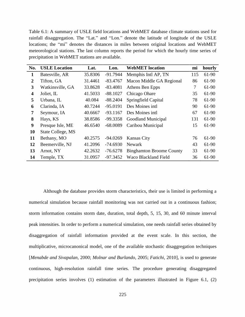
225

Table 6.1: A summary of USLE field locations and WebMET database climate stations used for

rainfall disaggregation. The “Lat.” and “Lon.” denote the latitude of longitude of the USLE

locations; the “mi” denotes the distances in miles between original locations and WebMET

meteorological stations. The last column reports the period for which the hourly time series of

precipitation in WebMET stations are available.

No. USLE Location

Lat.

Lon. WebMET location mi hourly

1 Batesville, AR 35.8306 -91.7944 Memphis Intl AP, TN 115 61-90

2 Tifton, GA 31.4461 -83.4767 Macon Middle GA Regional 86 61-90

3 Watkinsville, GA 33.8628 -83.4081 Athens Ben Epps 7 61-90

4 Joliet, IL 41.5033 -88.1027 Chicago Ohare 35 61-90

5 Urbana, IL 40.084 -88.2404 Springfield Capital 78 61-90

6 Clarinda, IA 40.7244 -95.0191 Des Moines intl 90 61-90

7 Seymour, IA 40.6667 -93.1167 Des Moines intl 67 61-90

8 Hays, KS 38.8586 -99.3358 Goodland Municipal 131 61-90

9 Presque Isle, ME 46.6540 -68.0089 Caribou Municipal 15 61-90

10 State College, MS

11 Bethany, MO 40.2575 -94.0269 Kansas City 76 61-90

12 Beemerville, NJ 41.2096 -74.6930 Newark 43 61-90

13 Arnot, NY 42.2632 -76.6278 Binghamton Broome County 33 61-90

14 Temple, TX 31.0957 -97.3452 Waco Blackland Field 36 61-90

Although the database provides storm characteristics, their use is limited in performing a

numerical simulation because rainfall monitoring was not carried out in a continuous fashion;

storm information contains storm date, duration, total depth, 5, 15, 30, and 60 minute interval

peak intensities. In order to perform a numerical simulation, one needs rainfall series obtained by

disaggregation of rainfall information provided at the event scale. In this section, the

multiplicative, microcanonical model, one of the available stochastic disaggregation techniques

[Menabde and Sivapalan, 2000; Molnar and Burlando, 2005; Fatichi, 2010], is used to generate

continuous, high-resolution rainfall time series. The procedure generating disaggregated

precipitation series involves (1) estimation of the parameters illustrated in Figure 6.1, (2)

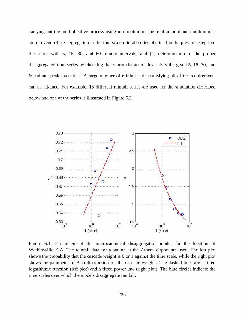
226

carrying out the multiplicative process using information on the total amount and duration of a

storm event, (3) re-aggregation to the fine-scale rainfall series obtained in the previous step into

the series with 5, 15, 30, and 60 minute intervals, and (4) determination of the proper

disaggregated time series by checking that storm characteristics satisfy the given 5, 15, 30, and

60 minute peak intensities. A large number of rainfall series satisfying all of the requirements

can be attained. For example, 15 different rainfall series are used for the simulation described

below and one of the series is illustrated in Figure 6.2.

Figure 6.1: Parameters of the microcanonical disaggregation model for the location of

Watkinsville, GA. The rainfall data for a station at the Athens airport are used. The left plot

shows the probability that the cascade weight is 0 or 1 against the time scale, while the right plot

shows the parameter of Beta distribution for the cascade weights. The dashed lines are a fitted

logarithmic function (left plot) and a fitted power law (right plot). The blue circles indicate the

time scales over which the models disaggregate rainfall.

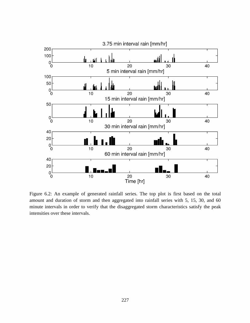
227

Figure 6.2: An example of generated rainfall series. The top plot is first based on the total

amount and duration of storm and then aggregated into rainfall series with 5, 15, 30, and 60

minute intervals in order to verify that the disaggregated storm characteristics satisfy the peak

intensities over these intervals.

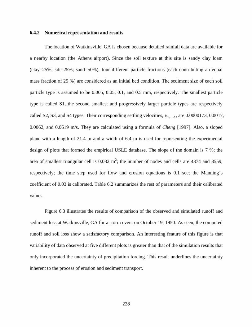
228

6.4.2 Numerical representation and results

The location of Watkinsville, GA is chosen because detailed rainfall data are available for

a nearby location (the Athens airport). Since the soil texture at this site is sandy clay loam

(clay=25%; silt=25%; sand=50%), four different particle fractions (each contributing an equal

mass fraction of 25 %) are considered as an initial bed condition. The sediment size of each soil

particle type is assumed to be 0.005, 0.05, 0.1, and 0.5 mm, respectively. The smallest particle

type is called S1, the second smallest and progressively larger particle types are respectively

called S2, S3, and S4 types. Their corresponding settling velocities, , are 0.0000173, 0.0017,

0.0062, and 0.0619 m/s. They are calculated using a formula of Cheng [1997]. Also, a sloped

plane with a length of 21.4 m and a width of 6.4 m is used for representing the experimental

design of plots that formed the empirical USLE database. The slope of the domain is 7 %; the

area of smallest triangular cell is 0.032 m2; the number of nodes and cells are 4374 and 8559,

respectively; the time step used for flow and erosion equations is 0.1 sec; the Manning‟s

coefficient of 0.03 is calibrated. Table 6.2 summarizes the rest of parameters and their calibrated

values.

Figure 6.3 illustrates the results of comparison of the observed and simulated runoff and

sediment loss at Watkinsville, GA for a storm event on October 19, 1950. As seen, the computed

runoff and soil loss show a satisfactory comparison. An interesting feature of this figure is that

variability of data observed at five different plots is greater than that of the simulation results that

only incorporated the uncertainty of precipitation forcing. This result underlines the uncertainty

inherent to the process of erosion and sediment transport.

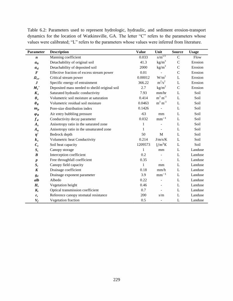
229

Table 6.2: Parameters used to represent hydrologic, hydraulic, and sediment erosion-transport

dynamics for the location of Watkinsville, GA. The letter “C” refers to the parameters whose

values were calibrated; “L” refers to the parameters whose values were inferred from literature.

Parameter Description Value Unit Source Usage

n Manning coefficient 0.033 s/m1/3

C Flow

Detachability of original soil

41.3 kg/m3 C Erosion

Detachability of deposited soil

2000 kg/m3 C Erosion

F Effective fraction of excess stream power

0.01 - C Erosion

Critical stream power

0.00012 W/m2 L Erosion

J Specific energy of entrainment

366.22 m2/s

2 L Erosion

Deposited mass needed to sheild original soil

2.7 kg/m

2 C Erosion

Saturated hydraulic conductivity 7.93 mm/hr L Soil

Volumetric soil moisture at saturation 0.414 m3 m

-3 L Soil

Volumetric residual soil moisture 0.0463 m3 m

-3 L Soil

Pore-size distribution index 0.1426 - L Soil

Air entry bubbling pressure -63 mm L Soil

Conductivity decay parameter 0.032 L Soil

Anisotropy ratio in the saturated zone 1 - L Soil

Anisotropy ratio in the unsaturated zone 1 - L Soil

Bedrock depth 50 M L Soil

Volumetric heat Conductivity 0.214 J/m/s/K L Soil

Soil heat capacity 1209573 L Soil

Ss Canopy storage 1 mm L Landuse

B Interception coefficient 0.2 - L Landuse

p Free throughfall coefficient 0.35 - L Landuse

Sc Canopy field capacity 1 mm L Landuse

K Drainage coefficient 0.18 mm/h L Landuse

gd Drainage exponent parameter 3.9 L Landuse

alb Albedo 0.22 - L Landuse

Hv Vegetation height 0.46 - L Landuse

Kt Optical transmission coefficient 0.7 - L Landuse

rs Reference canopy stomatal resistance 200 s/m L Landuse

Vf Vegetation fraction 0.5 - L Landuse

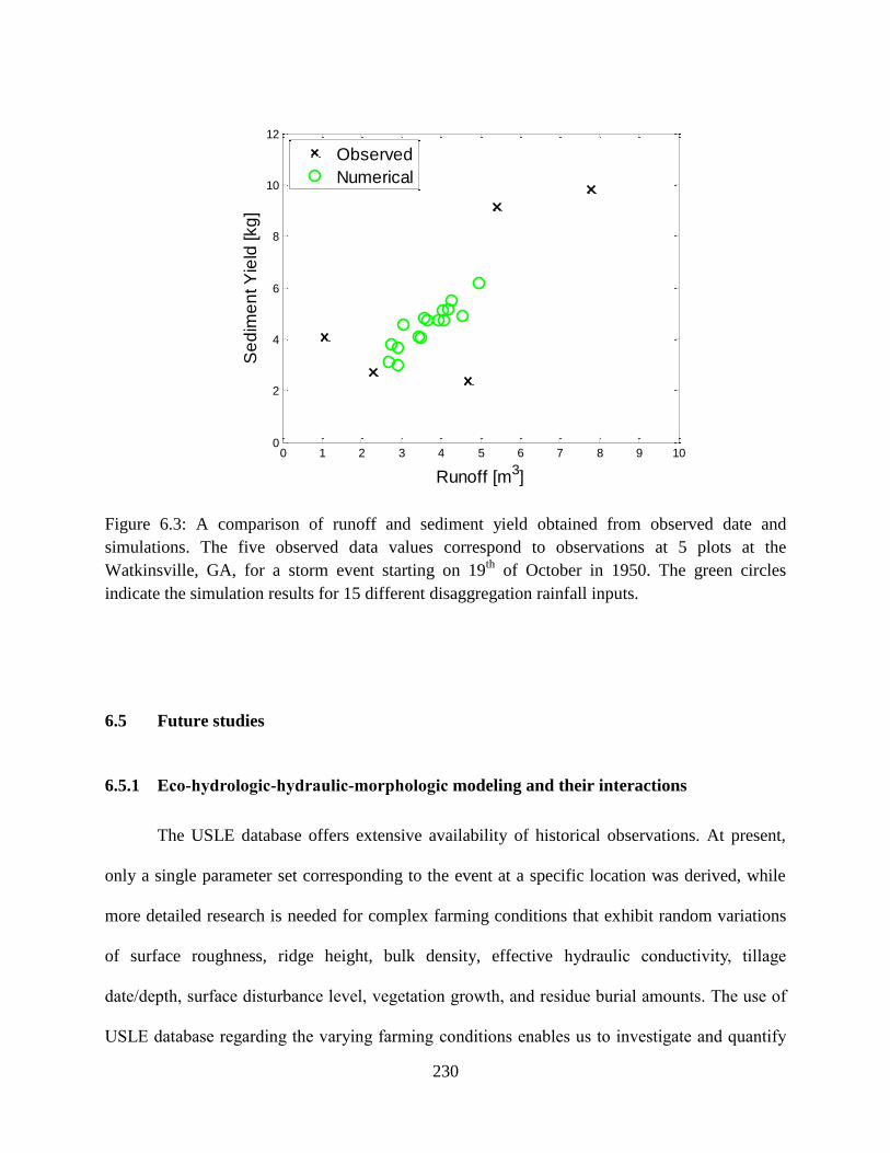
230

Figure 6.3: A comparison of runoff and sediment yield obtained from observed date and

simulations. The five observed data values correspond to observations at 5 plots at the

Watkinsville, GA, for a storm event starting on 19th

of October in 1950. The green circles

indicate the simulation results for 15 different disaggregation rainfall inputs.

6.5 Future studies

6.5.1 Eco-hydrologic-hydraulic-morphologic modeling and their interactions

The USLE database offers extensive availability of historical observations. At present,

only a single parameter set corresponding to the event at a specific location was derived, while

more detailed research is needed for complex farming conditions that exhibit random variations

of surface roughness, ridge height, bulk density, effective hydraulic conductivity, tillage

date/depth, surface disturbance level, vegetation growth, and residue burial amounts. The use of

USLE database regarding the varying farming conditions enables us to investigate and quantify

0 1 2 3 4 5 6 7 8 9 100

2

4

6

8

10

12

Runoff [m3]

Se

dim

en

t Y

ield

[kg

]

Observed

Numerical

231

the soil-terrain-vegetation interactions of watershed systems. However, numerical representation

of such conditions is very challenging because it is involved with feasibilities of several

processes of flow, subsurface, and vegetation; thus can only become a reality under the multi-

scale, coupled approach proposed in this dissertation. In the future study, numerical simulations

with all eco-hydrological-hydraulic-morphologic components will be addressed as one of the

most fruitful topics. How important is a fully consideration of connected watershed systems in

quantifying the response of the morphologic variations in future climates? What is the role of

vegetation in the sedimentary dynamics? Does vegetation influence hydrologic partitioning of

water and energy, converging and diverging flow and sediment movements, and their

accumulation behind a clump of vegetation? Also, how can topographic characteristics of

domain affect morphologic features? Do north-facing hillslopes increase erosion or deposition?

Is this phenomenon because of different vegetation due to opposing climate conditions?

6.5.2 Future assessment studies with uncertainty analyses under climate change

Another prospective of the future studies is to investigate the uncertainty and non-

linearities of morphologic responses for the climatologic signals given in a watershed system.

Due to feedback and compensatory processes as well as the dissipative nature of watersheds, the

key to a breakthrough in predictive capabilities lies in an integrated, interdisciplinary approach,

whereby the physically-based model can be used for climate impact evaluations. The processes

involved in the propagation of climate signals are characterized by such vastly different spatial

and temporal scales with high non-linearities. As mentioned previously, any response to the

forcings such as precipitation and temperature showed a highly varying, sometimes contradictory

result, but sufficient explanations for the result were not discussed yet. How can we characterize

232

uncertainty and non-linearities associated with projections of climate change impact on

watershed systems? How do large-scale processes affect variables at the scales relevant to human

actions and ecosystem services? To answer the questions, the following elements will be

explicitly addressed in future assessment studies: (1) the uncertainty of climate projections, as

inferred from an ensemble of GCM realizations [Note: the current generation of Global

Circulation Models (GCMs) exhibits a large degree of uncertainty in simulation of precipitation,

the primary hydrological driver; the typical ad hoc selection of a given GCM for impact

evaluations introduces subjectivity into the assessment process]; (2) the uncertainty of

hydrological simulation [Note: a single hydrological model is typically used in assessments

because of lack of standardized physically-based models; uncertainty estimation has to

accompany inferences of a single-model assessment]; (3) when precipitation extremes are

concerned, alternative approaches to their projection into future need to be accounted for [Note:

both GCMs and Regional Climate Models (RCMs) do not capture extremes well]; (4) the

dynamic nature of vegetation has to be accounted for [Note: currently, hydrological assessments

do not represent the physiological response of vegetation to longer growing seasons, warmer

conditions, and atmosphere enriched with CO2, a potentially important feedback from the land-

surface]; and, importantly, (5) the hydrological impacts of climate change need to be represented

at a range of spatiotemporal scales (multi-scale), in particular, at those relevant to the scales of

human actions and ecosystem services [Note: similar to the concept of a using a finer-resolution

RCM forced with boundary conditions of a coarser-scale GCM, a nested, multi-scale approach to

assessments in hydrological modeling will generate features emerging from atmosphere-

vegetation-soil-streamflow processes, which will be dynamically consistent with boundary

233

conditions generated by a coarser watershed-scale model. All these elements will be addressed in

the future studies.

6.5.3 A longer time simulation with a parallel mode

This study was one of the first who addressed the interactions between the watershed

components. Chapter III was to identify the effects of topography on morphologic behaviors;

Chapter IV was to quantify the interactions between flow and vegetation; Chapter V was to

investigate the effects of climatological forcing on morphologic variations. These Chapters, by

assuming the bed condition as impermeable and considering vegetation growths as static,

focused on a short-term response between the processes and did not fully take hydrological

effects or vegetation dynamics into account at long-term scales due to the constrained time step.

Since a longer time simulation helps us to understand valuable information on the seasonal

patterns or cycles of hydrologic, morphologic, hydraulic variables, we need to extend feasibility

of the model to the longer time simulation. However, unfortunately, the long-term simulations in

serial mode are not currently feasible because of a limited computing power and the inherent

feature of the adopted numerical scheme. Therefore, for attempting to trade off the accuracy of

the numerical model against the efficiency, a promising alternative is to perform the model with

a parallel mode. One of the future directions will be focused on overcoming the constraint of

temporal scale by means of a parallelized code.

234

APPENDIX A

Error Indices

A.1 Error Indices

1. Peak flow error (PFE, [%])

|

|

2. Phase error (PE, [hour])

3. Volume error (VE, [%])

| |

4. Root mean square error (RMSE, )

√∑ (

)

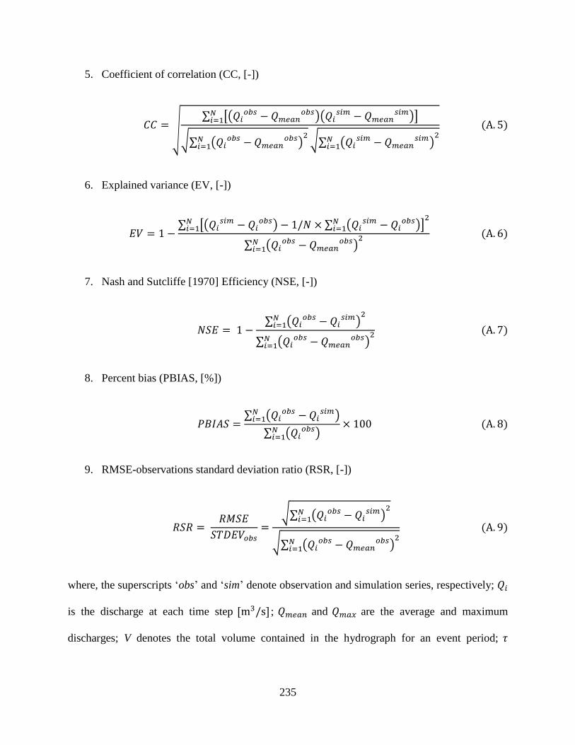
235

5. Coefficient of correlation (CC, [-])

√

∑ [(

)(

)]

√∑ (

)

√∑ (

)

6. Explained variance (EV, [-])

∑ [(

) ∑ (

)

]

∑ (

)

7. Nash and Sutcliffe [1970] Efficiency (NSE, [-])

∑ (

)

∑ (

)

8. Percent bias (PBIAS, [%])

∑ (

)

∑ ( )

9. RMSE-observations standard deviation ratio (RSR, [-])

√∑ (

)

√∑ (

)

where, the superscripts „obs‟ and „sim‟ denote observation and simulation series, respectively;

is the discharge at each time step ; and are the average and maximum

discharges; V denotes the total volume contained in the hydrograph for an event period;

236

denotes the time when the peak discharge is reached; N is a total number of values within the

time period of an event.

237

APPENDIX B

Eigenvalues and eigenvectors of Jacobian

B.1 Jacobian

For the purpose of evaluating the flux using the Roe‟s approximate Riemann solver, the

Jacobian of the normal flux ( ) can be first computed as

The conservative variable vector, U and x- and y- directional flux vectors, E and G can be

explicitly written as

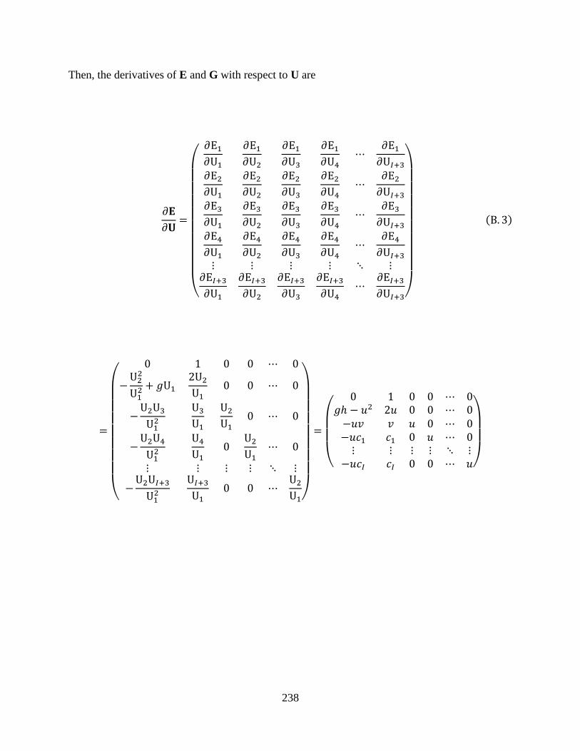
238

Then, the derivatives of E and G with respect to U are

(

)

(

)

(

)

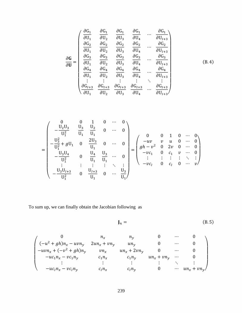
239

(

)

(

)

(

)

To sum up, we can finally obtain the Jacobian following as

(

)

240

B.2 Eigenvalues and Eigenvectors

To obtain the eigenvalue of the square matrix, Jacobian, we need to find numbers

satisfying the following relation:

| |

This determinant shows the order of I+3 so that it has the same number of roots. The computed

roots corresponding to eigenvalues are:

| |

(

| |

| |

| |

| |

| |)

The introduction of matrices with a single column can be used for the computation of

right-eigenvector (R). From the following definition

(

(

( ) ( )

( ) ( )

( )

( ) )

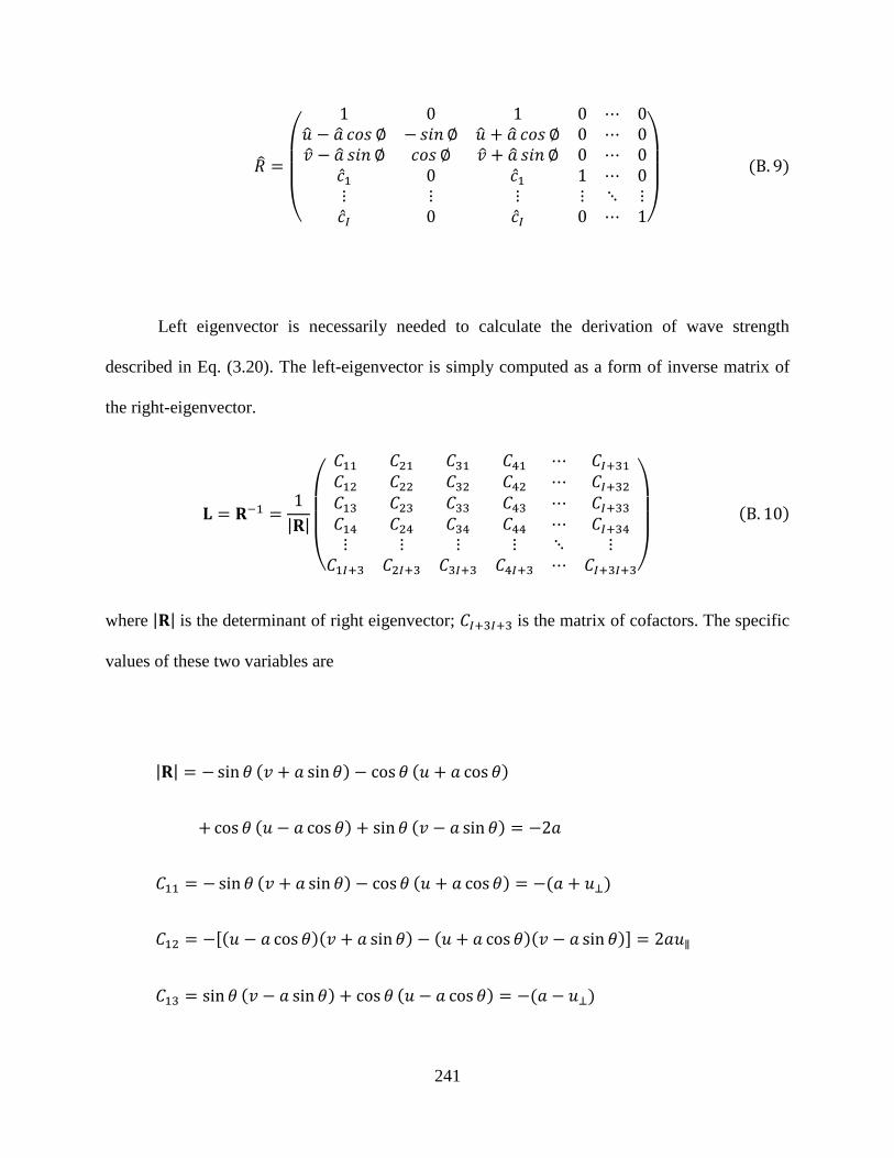
241

(

)

Left eigenvector is necessarily needed to calculate the derivation of wave strength

described in Eq. (3.20). The left-eigenvector is simply computed as a form of inverse matrix of

the right-eigenvector.

| |

(

)

where | | is the determinant of right eigenvector; is the matrix of cofactors. The specific

values of these two variables are

| |

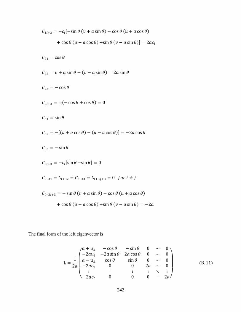
242

The final form of the left eigenvector is

(

)

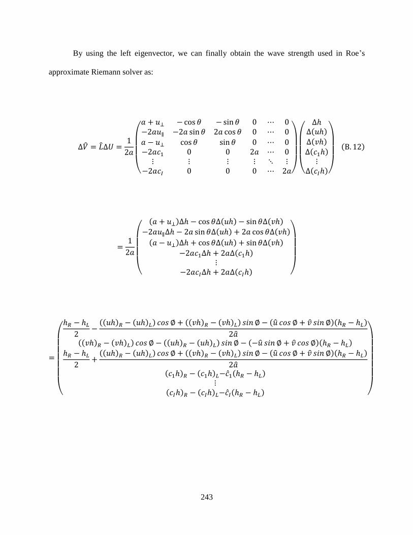
243

By using the left eigenvector, we can finally obtain the wave strength used in Roe‟s

approximate Riemann solver as:

(

)

(

)

(

)

(

)

244

NOTATION

Parameter Description

A area of triangular cell

Ar area of roughness element

anisotropy ratio in the saturated zone

anisotropy ratio in the unsaturated zone

a celerity

a0 detachability of original soil

ad detachability of deposited soil

alb surface albedo

B interception coefficient

b exponent used in Eq. (3.9)

C Chezy resistance factor

CD bed drag coefficient

Cr Courant number

soil heat capacity

ci sediment concentration

D erosion rates vector

DR mean raindrop size

Dr diameter of roughness element

D50 median particle size

di deposition rate

E x-directional flux vector

Ex summation of bed elevation, depth, and velocity head

ei rainfall driven detachment rate

eri rainfall driven redetachment rate

F flux vector

F effective fraction of excess stream power

Fw shield effect factor

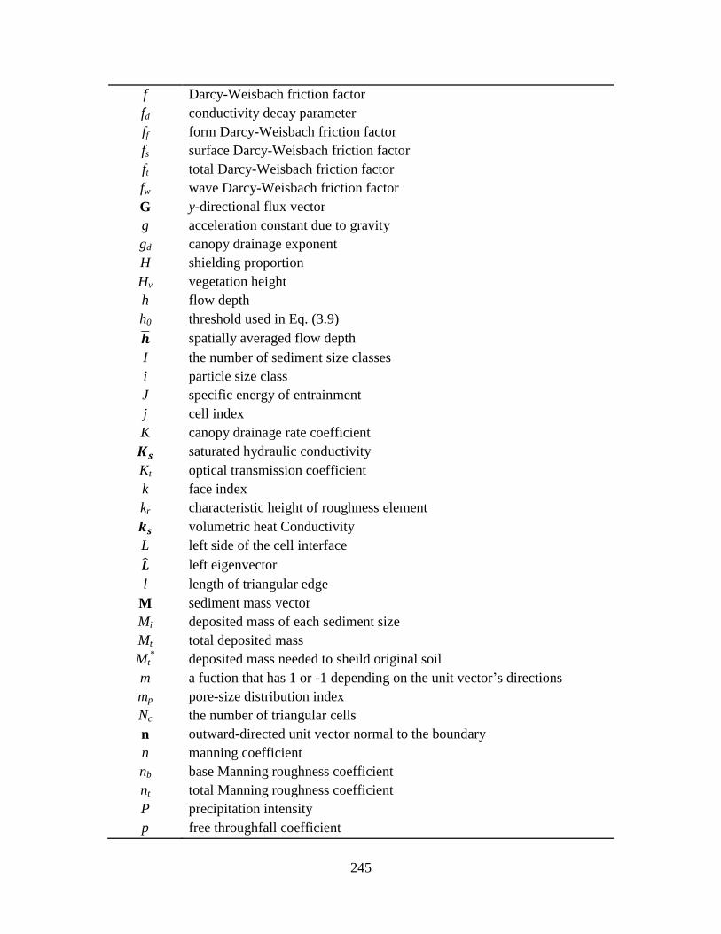
245

f Darcy-Weisbach friction factor

fd conductivity decay parameter

ff form Darcy-Weisbach friction factor

fs surface Darcy-Weisbach friction factor

ft total Darcy-Weisbach friction factor

fw wave Darcy-Weisbach friction factor

G y-directional flux vector

g acceleration constant due to gravity

gd canopy drainage exponent

H shielding proportion

Hv vegetation height

h flow depth

h0 threshold used in Eq. (3.9)

spatially averaged flow depth

I the number of sediment size classes

i particle size class

J specific energy of entrainment

j cell index

K canopy drainage rate coefficient

saturated hydraulic conductivity

Kt optical transmission coefficient

k face index

kr characteristic height of roughness element

volumetric heat Conductivity

L left side of the cell interface

left eigenvector

l length of triangular edge

M sediment mass vector

Mi deposited mass of each sediment size

Mt total deposited mass

Mt* deposited mass needed to sheild original soil

m a fuction that has 1 or -1 depending on the unit vector‟s directions

mp pore-size distribution index

Nc the number of triangular cells

n outward-directed unit vector normal to the boundary

n manning coefficient

nb base Manning roughness coefficient

nt total Manning roughness coefficient

P precipitation intensity

p free throughfall coefficient

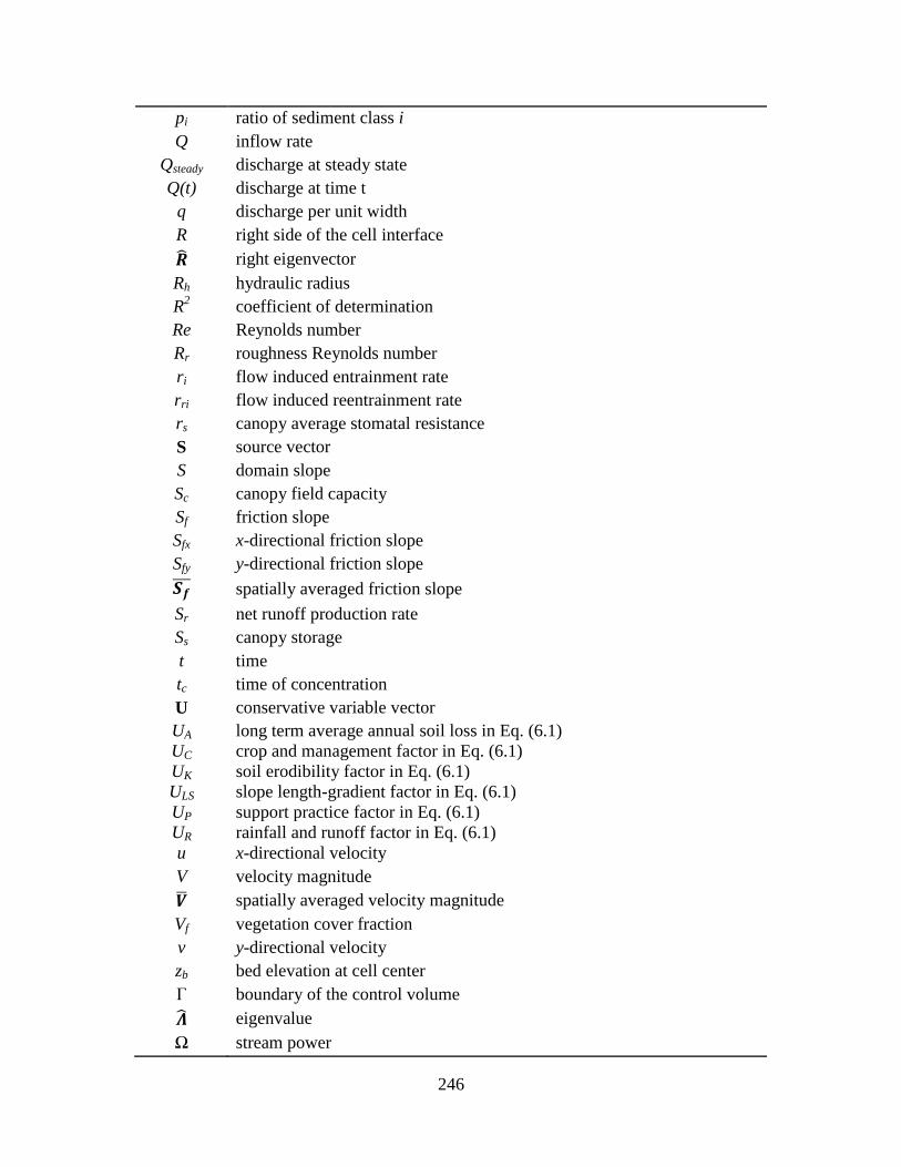
246

pi ratio of sediment class i

Q inflow rate

Qsteady discharge at steady state

Q(t) discharge at time t

q discharge per unit width

R right side of the cell interface

right eigenvector

Rh hydraulic radius

R2 coefficient of determination

Re Reynolds number

Rr roughness Reynolds number

ri flow induced entrainment rate

rri flow induced reentrainment rate

rs canopy average stomatal resistance

S source vector

S domain slope

Sc canopy field capacity

Sf friction slope

Sfx x-directional friction slope

Sfy y-directional friction slope

spatially averaged friction slope

Sr net runoff production rate

Ss canopy storage

t time

tc time of concentration

U conservative variable vector

UA long term average annual soil loss in Eq. (6.1)

UC crop and management factor in Eq. (6.1)

UK soil erodibility factor in Eq. (6.1)

ULS slope length-gradient factor in Eq. (6.1)

UP support practice factor in Eq. (6.1)

UR rainfall and runoff factor in Eq. (6.1)

u x-directional velocity

V velocity magnitude

spatially averaged velocity magnitude

Vf vegetation cover fraction

v y-directional velocity

zb bed elevation at cell center

Γ boundary of the control volume

eigenvalue

Ω stream power

247

Ωcr critical stream power

Ωx x-directional stream power

Ωy y-directional stream power

angle between the face normal vector and the x axis

β porosity of bed

c critical Shields parameter for incipient motion

volumetric residual soil moisture

volumetric soil moisture at saturation

air entry bubbling pressure

bedrock depth

νR rainfall impact velocity

μ dynamic viscosity of water

ρs density of sediment

ρw density of water

λ eigenvalue

ϵ a tolerance value used in Eq. (4.1)

∆ finite difference across the interface

wave strength

248

BIBLIOGRAPHY

Abbott, M. B. (1974), Continuous flows, discontinuous flows and numerical analysis, Journal of

Hydraulic Research, 12(4), 417-467.

Abrahams, A. D., and A. J. Parsons (1994), Hydraulics of interrill overland-flow on stone-

covered desert surfaces, Catena, 23(1-2), 111-140.

Abrahams, A. D., A. J. Parsons, and S. H. Luk (1986), Resistance to overland-flow on desert

hillslopes, J. Hydrol., 88(3-4), 343-363.

Abu Hammad, A. H., T. Børresen, and L. E. Haugen (2006), Effects of rain characteristics and

terracing on runoff and erosion under the Mediterranean, Soil and Tillage Research,

87(1), 39-47.

Ahmadi, A., M. R. Neyshabouri, H. Rouhipour, H. Asadi, and M. Irannajad (2010), Factors and

mechanisms influencing interrill erodibility at different rainfall intensities, Journal of

Food, Agriculture & Environment, 8(2), 996-999.

Akanbi, A. A., and N. D. Katopodes (1988), Model for flood propapation on initially dry land,

edited, pp. 689-706, Journal of Hydraulic Engineering-ASCE.

Aksoy, H., and M. L. Kavvas (2005), A review of hillslope and watershed scale erosion and

sediment transport models, CATENA, 64(2-3), 247-271.

Alonso, R., M. Santillana, and C. Dawson (2008), On the diffusive wave approximation of the

shallow water equations, European Journal of Applied Mathematics, 19, 575-606.

Anderson, J. D. (1995), Computational Fluid Dynamics, McGraw–Hill, New York.

Armstrong, A., J. N. Quinton, B. C. P. Heng, and J. H. Chandler (2011), Variability of interrill

erosion at low slopes, Earth Surface Processes and Landforms, 36(1), 97-106.

Armstrong, A., J. N. Quinton, B. C. P. Heng, and G. C. Sander (2012), Processes controlling the

development of a shielding layer on natural soil, European Journal of Soil Science, 63(1),

54-64.

Arnell, N. W. (2003), Effects of IPCCSRES emissions scenarios on river runoff: a global

perspective, Hydrology and Earth System Sciences, 7(5), 619-641.

Bagnold, R. A. (1966), An approach to the sediment transport problem for general physics,

Geological Survey Professional Paper (U.S.), 442-I.

Bai, Z. G., D. L. Dent, L. Olsson, and M. E. Schaepman (2008), Proxy global assessment of land

degradation, Soil Use and Management, 24, 223-234.

Baird, W. F. (2001), Muskegon river delta - Role of the cobb plant discharge channel structure,

Report to Consumers Energy.

249

Barnett, T. P., J. C. Adam, and D. P. Lettenmaier (2005), Potential impacts of a warming climate

on water availability in snow-dominated regions, Nature, 438, 303-309.

Begnudelli, L., and B. F. Sanders (2006), Unstructured grid finite-volume algorithm for shallow-

water flow and scalar transport with wetting and drying, Journal of Hydraulic

Engineering-ASCE, 132(4), 371-384.

Begnudelli, L., and B. F. Sanders (2007), Simulation of the St. Francis dam-break flood, Journal

of Engineering Mechanics-ASCE, 133, 1200-1212.

Begnudelli, L., B. F. Sanders, and S. F. Bradford (2008), Adaptive Godunov-based model for

flood simulation, Journal of Hydraulic Engineering-ASCE, 134(6), 714-725.

Beuselinck, L., G. Govers, A. Steegen, and P. B. Hairsine (1998), Experiments on sediment

deposition by overland flow, Modelling Soil Erosion, Sediment Transport and Closely

Related Hydrological Processes(249), 91-96.

Beuselinck, L., G. Govers, A. Steegen, and T. A. Quine (1999), Sediment transport by overland

flow over an area of net deposition, Hydrological Processes, 13(17), 2769-2782.

Biron, P. M., S. N. Lane, A. G. Roy, K. F. Bradbrook, and K. S. Richards (1998), Sensitivity of

bed shear stress estimated from vertical velocity profiles: the problem of sampling

resolution., Earth Surface Processes and Landforms, 23, 133-139.

Bissonnais, Y. L., B. Renaux, and H. Delouche (1995), Interactions between soil properties and

moisture content in crust formation, runoff and interrill erosion from tilled loess soils,

CATENA, 25(1-4), 33-46.

Bixio, A. C., M. Putti, S. Orlandini, and C. Paniconi (2000), Physically-based distributed model

for coupled surface runoff and subsurface flow simulation at the catchment scale,

Computational Methods in Water Resources, 1115-1122.

Blasius, H. (1913), Das Ähnlichkeitsgesetz bei Reibungsvorgängen in Flüssigkeiten,

Forschungs-Arbeit des Ingenieur-Wesens, 131, 1-41.

Bradford, S. F., and N. D. Katopodes (1999), Hydrodynamics of turbid underflows. I:

Formulation and numerical analysis, Journal of Hydraulic Engineering-ASCE, 125(10),

1006-1015.

Bradford, S. F., and N. D. Katopodes (2001), Finite volume model for nonlevel basin irrigation,

Journal of Irrigation and Drainage Engineering-ASCE, 127(4), 216-223.

Bradford, S. F., and B. F. Sanders (2002), Finite-volume model for shallow-water flooding of

arbitrary topography, Journal of Hydraulic Engineering-ASCE, 128(3), 289-298.

Bras, R. L. (1990), Hydrology: an Introduction to Hydrologic Science., Addison-

Wesley/Longman, Reading, MA/London.

Brown, L. R. (1984), Conserving soils., State of the world, L. R. Brown, ed., Norton, New York,

53-75.

Brufau, P., and P. Garcia-Navarro (2003), Unsteady free surface flow simulation over complex

topography with a multidimensional upwind technique, Journal of Computational

Physics, 186(2), 503-526.

Brufau, P., P. Garcia-Navarro, and M. E. Vazquez-Cendon (2004), Zero mass error using

unsteady wetting-drying conditions in shallow flows over dry irregular topography,

International Journal of Numerical Methods in Fluids, 45(10), 1047-1082.

Bunn, S. E., and A. H. Arthington (2002), Basic principles and ecological consequences of

altered flow regimes for aquatic biodiversity, Environmental Management, 30(4), 492-

507.

250

Bunte, K., and J. Poesen (1993), Effects of rock fragment covers on erosion and transport of

noncohesive sediment by shallow overland flow, Water Resources Research, 29, 1415-

1424.

Buringh, P. (1981), An assessment of losses and degradation of productive agricultural land in

the world, FAO Working Group on Soils Policy, Rome.

Cabral, M. C., L. Garrote, R. L. Bras, and D. Entekhabi (1992), A kinematic model of infiltration

and runoff generation in layered and sloped soils, Advances in Water Resources, 15,

311-324.

Camporese, M., C. Paniconi, M. Putti, and S. Orlandini (2010), Surface-subsurface flow

modeling with path-based runoff routing, boundary condition-based coupling, and

assimilation of multisource observation data, Water Resources Research, 46, W02512,

doi:10.1029/2008WR007536.

Cao, Z., R. Day, and S. Egashira (2002), Coupled and decoupled numerical modeling of flow

and morphological evolution in alluvial rivers, Journal of Hydraulic Engineering-ASCE,

128(3), 306-321.

Cao, Z., G. Pender, S. Wallis, and P. Carling (2004), Computational dam-break hydraulics over

erodible sediment bed, Journal of Hydraulic Engineering-ASCE, 130(7), 689-703.

Chen, X., J. Wu, and Q. Hu (2008), Simulation of climate change impacts on streamflow in the

Bosten lake basin using an artificial neural network model, Journal of Hydrologic

Engineering, 13(3), 180-183.

Cheng, N. (1997), Simplified settling velocity formula for sediment particle, Journal of

Hydraulic Engineering-ASCE, 123(2), 149-152.

Cherkauer, A., and T. Sinha (2010), Hydrologic impacts of projected future climate change in

the Lake Michigan region, Journal of Great Lakes Research, 36, 33-50.

Chow, V. T. (1959), Open-channel Hydraulics, McGraw-Hill Book Co., New York, N.Y., 680 pp.

Cowan, W. L. (1956), Estimating hydraulic roughness coefficients, Agricultural Engineering,

37(7), 473-475.

Dankers, R., and L. Feyen (2008), Climate change impact on flood hazard in Europe: An

assessment based on high-resolution climate simulations, Journal of Geophysical

Research-Atmospheres, 113(D19).

De Roo, A. P. J., L. Hazelhoff, and P. A. Burrough (1989), Soil erosion modelling using

„ANSWERS‟ and geographical information systems, Earth Surface Processes and

Landforms, 14, 517-532.

Deardorff, J. W. (1978), Efficient prediction of ground surface temperature and moisture, with

inclusion of a layer of vegetation, Journal of Geophysical Research, 83(C4), 1889-1903.

Defersha, M. B., and A. M. Melesse (2012), Field-scale investigation of the effect of land use on

sediment yield and runoff using runoff plot data and models in the Mara River basin,

Kenya, CATENA, 89, 54-64.

Defersha, M. B., S. Quraishi, and A. Melesse (2011), The effect of slope steepness and

antecedent moisture content on interrill erosion, runoff and sediment size distribution in

the highlands of Ethiopia, Hydrology and Earth System Sciences, 15, 2367-2375.

DiGiammarco, P., E. Todini, and P. Lamberti (1996), A conservative finite elements approach to

overland flow: The control volume finite element formulation, J. Hydrol., 175(1-4), 267-

291.

Downer, C. W., and F. L. Ogden (2004), GSSHA: Model to simulate diverse stream flow

producing processes, Journal of Hydrologic Engineering, 9(3), 161-174.

251

Du, J. K., S. P. Xie, Y. P. Xu, C. Y. Xu, and V. P. Singh (2007), Development and testing of a

simple physically-based distributed rainfall-runoff model for storm runoff simulation in

humid forested basins, J. Hydrol., 336(3-4), 334-346.

Dunne, T., and R. D. Black (1970), An experimental investigation of runoff production in

permeable soils, Water Resources Research, 6(2), 478-490.

Edwards, W. M., and L. B. Owens (1991), Large storm effects on total soil erosion, Journal of

Soil and Water Conservation, 46(1), 75-78.

Einstein, H. A., and R. B. Banks (1950), Fluid resistance of composite roughness, Transactions

of the American Geophysics Union, 31(4), 603-610.

Eltahir, E. A. B., and R. L. Bras (1993), A description of rainfall interception over large areas,

Journal of Climate, 6, 1002-1008.

Emmett, W. W. (1970), The hydraulics of overland flow on hillslopes, U.S. Geological Survey,

Prof. Paper 662-A, 68 pp.

Entekhabi, D. (2000), Land Surface Processes: Basic Tools and Concepts., Department of Civil

and Environmental Engineering, MIT, Cambridge, MA.

Fathi-Moghadam, M. (2006), Effects of Land Slope and Flow Depth on Retarding Flow in Non-

submerge Vegetated Lands, Journal of Agronomy, 5, 536-540.

Fatichi, S. (2010), The Modeling of Hydrological Cycle and its Interaction with Vegetation in

the Framework of Climate Change, ph.D dissertation, University of Firenze.

Ferro, V. (2003), Flow resistance in gravel-bed channels with large-scale roughness, Earth

Surface Processes and Landforms, 28, 1325-1339.

Fiener, P., G. Govers, and K. Van Oost (2008), Evaluation of a dynamic multi-class sediment

transport model in a catchment under soil-conservation agriculture, Earth Surface

Processes and Landforms, 33(11), 1639-1660.

Francipane, A., V. Y. Ivanov, L. V. Noto, E. Istanbulluoglu, E. Arnone, and R. L. Bras (2012),

tRIBS-Erosion: A parsimonious physically-based model for studying catchment hydro-

geomorphic response, CATENA, 92(0), 216-231.

Gao, B., M. T. Walter, T. S. Steenhuis, J. Y. Parlange, K. Nakano, C. W. Rose, and W. L.

Hogarth (2003), Investigating ponding depth and soil detachability for a mechanistic

erosion model using a simple, J. Hydrol., 277(1-2), 116-124.

Gilley, J. E., and S. C. Finkner (1991), Hydraulic roughness coefficients as affected by random

roughness, Transactions of American Society of Agricultural Engineers, 34(3), 897-903.

Gilley, J. E., E. R. Kottwitz, and G. A. Wieman (1992a), Darcy-Weisbach roughness coefficients

for gravel and cobble surfaces, Journal of Irrigation and Drainage Engineering-ASCE,

118, 104-112.

Gilley, J. E., D. Flanagan, E. R. Kottwitz, and M. A. Weltz (1992b), Darcy-Weisbach roughness

coefficients for overland flow, In Parsons, A. J. and Abrahams, A.D., editors, Overland

flow, London: UCL Press, 25-52.

Goderniaux, P., S. Brouyere, H. J. Fowler, S. Blenkinsop, R. Therrien, P. Orban, and A.

Dassargues (2009), Large scale surface–subsurface hydrological model to assess climate

change impacts on groundwater reserves, J. Hydrol., 373, 122-138.

Goodrich, D. C., T. O. Keefer, C. L. Unkrich, M. H. Nichols, H. B. Osborn, J. J. Stone, and J. R.

Smith (2008), Long-term precipitation database, Walnut Gulch Experimental Watershed,

Arizona, United States, Water Resources Research, 44(5).

Gottardi, G., and M. Venutelli (2008), An accurate time integration method for simplified

overland flow models, Advances in Water Resources, 31(1), 173-180.

252

Govindaraju, R. S., M. L. Kavvas, and S. E. Jones (1990), Approximate analytical solutions for

overland flows, Water Resources Research, 26(12), 2903-2912.

Gutiérrez-Jurado, H. A., E. R. Vivoni, E. Istanbulluoglu, and R. L. Bras (2007), Ecohydrological

response to a geomorphically significant flood event in a semiarid catchment with

contrasting ecosystems, Geophysical Research Letters 34, L24S25.

Hairsine, P. B., and C. W. Rose (1991), Rainfall detachment and deposition: Sediment transport

in the absence of flow-driven processes, Soil Science Society of America Journal, 55(2),

320-324.

Hairsine, P. B., and C. W. Rose (1992), Modeling water erosion due to overland flow using

physical principles: 1. Sheet flow, Water Resources Research, 28(1), 237-243.

Hairsine, P. B., L. Beuselinck, and G. C. Sander (2002), Sediment transport through an area of

net deposition, Water Resources Research, 38(6).

Hairsine, P. B., G. C. Sander, C. W. Rose, J. Y. Parlange, W. L. Hogarth, I. Lisle, and H.

Rouhipour (1999), Unsteady soil erosion due to rainfall impact: a model of sediment

sorting on the hillslope, J. Hydrol., 220(3-4), 115-128.

Harmel, R. D., J. V. Bonta, and C. W. Richardson (2007), The original USDA-ARS

experimental watersheds in Texas and Ohio: contributions from the past and visions for

the future, Transactions of the American Society of Agricultural and Biological

Engineers, 50(5), 1669-1675.

Harmel, R. D., C. W. Richardson, K. W. King, and P. M. Allen (2006), Runoff and soil loss

relationships for the Texas Blackland Prairies ecoregion, J. Hydrol., 331, 471-483.

HEC (1998), HEC-1 Flood Hydrograph Package User's Manual version 4.1, US ARMY CORPS

OF ENGINEERS, Hydrologic Engineering Center.

Heilig, A., D. DeBruyn, M. T. Walter, C. W. Rose, J. Y. Parlange, T. S. Steenhuis, G. C. Sander,

P. B. Hairsine, W. L. Hogarth, and L. P. Walker (2001), Testing a mechanistic soil

erosion model with a simple experiment, J. Hydrol., 244(1-2), 9-16.

Heng, B. C. P., G. C. Sander, and C. F. Scott (2009), Modeling overland flow and soil erosion on

nonuniform hillslopes: A finite volume scheme, Water Resources Research, 45.

Heng, B. C. P., G. C. Sander, A. Armstrong, J. N. Quinton, J. H. Chandler, and C. F. Scott

(2011), Modeling the dynamics of soil erosion and size-selective sediment transport over

nonuniform topography in flume-scale experiments, Water Resources Research, 47.

Hessel, R., V. Jetten, and Z. Guanghui (2003), Estimating Manning‟s n for steep slopes, Catena,

54, 77-91.

Hirsch, C. (1990), Numerical computation of internal and external flows, John Wiley & Sons,

New York.

Hirsch, P. (1996), Hydraulic resistance to overland flow on semiarid hillslopes: A physical

simulation, Ph.D. thesis, State University of New York at Buffalo.

Hogarth, W. L., C. W. Rose, J. Y. Parlange, G. C. Sander, and G. Carey (2004a), Soil erosion

due to rainfall impact with no inflow: a numerical solution with spatial and temporal

effects of sediment settling velocity characteristics, J. Hydrol., 294(4), 229-240.

Hogarth, W. L., J. Y. Parlange, C. W. Rose, G. C. Sander, T. S. Steenhuis, and A. Barry (2004b),

Soil erosion due to rainfall impact with inflow: an analytical solution with spatial and

temporal effects, J. Hydrol., 295(1-4), 140-148.

Horritt, M. S. (2002), Evaluating wetting and drying algorithms for finite element models of

shallow water flow, International Journal for Numerical Methods in Engineering, 55(7),

835-851.

253

Horton, R. E. (1933), The role of infiltration in the hydrological cycle, Transactions, American

Geophysical Union, 14, 446-460.

Howes, D. A., A. D. Abrahams, and E. B. Pitman (2006), One- and two-dimensional modelling

of overland flow in semiarid shrubland, Jornada basin, New Mexico, Hydrological

Processes, 20(5), 1027-1046.

Hromadka, T. V., and A. J. Nestlinger (1985), Technical note - Estimating watersheds-graphs

using a diffusion flow model, Advances in Water Resources, 8(4), 214-218.

Hromadka, T. V., C. E. Berenbrock, J. R. Freckleton, and G. L. Guymon (1985), A two-

dimensional dam-break flood-plain model, Advances in Water Resources, 8(1), 7-14.

Hu, S. X., and A. D. Abrahams (2006), Partitioning resistance to overland flow on rough mobile

beds, Earth Surface Processes and Landforms, 31(10), 1280-1291.

Hu, Z., and S. Islam (1995), Prediction of ground surface temperature and soil moisture content

by the force-restore method., Water Resources Research, 31(10), 2531-2539.

Huang, C., L. K. Wells, and L. D. Norton (1999), Sediment transport capacity and erosion

processes: Model concepts and reality, Earth Surface Processes and Landforms, 24(6),

503-516.

Huang, J. K., and K. T. Lee (2009), Influences of spatially heterogeneous roughness on flow

hydrographs, Advances in Water Resources, 32(11), 1580-1587.

Hunter, N. M., P. D. Bates, M. S. Horritt, and M. D. Wilson (2007), Simple spatially-distributed

models for predicting flood inundation: A review, Geomorphology, 90(3-4), 208-225.

Hursh, C. R., and E. F. Brater (1941), Separating storm-hydrographs from small drainage-areas

into surface and subsurface flow, Transactions, American Geophysical Union, 22, 863-

870.

IPCC (Intergovernmental Panel on Climate Change) (2001), Climate Change 2001: The

Scientific Basis, Contribution of Working Group I to the Third Assessment Report of the

Intergovernmental Panel on Climate Change, [Houghton, J.T.,Y. Ding, D.J. Griggs,4 M.

Noguer, P.J. van der Linden, X. Dai, K. Maskell, and C.A. Johnson (eds.)]. Cambridge

University Press, Cambridge, United Kingdom and New York, NY, USA, 881pp.

IPCC (Intergovernmental Panel on Climate Change) (2007), Climate Change: The Physical

Science Basis. In: Solomon, S., Qin, D., Manning, M., Chen, Z., Marquis, M., Avery,

K.B., Tignor, M., Miller, H.L. (Eds.), Contribution of Working Group 1 to the Fourth

Assessment Report of the Intergovernmental Panel on Climate Change, Cambridge Univ.

Press, Cambridge, UK.

Istanbulluoglu, E., O. Yetemen, E. R. Vivoni, H. A. Gutierrez-Jurado, and R. L. Bras (2008),

Eco-geomorphic implications of hillslope aspect: Inferences from analysis of landscape

morphology in central New Mexico, Geophysical Research Letters, 35(14).

Ivanov, V. Y., E. R. Vivoni, R. L. Bras, and D. Entekhabi (2004a), Catchment hydrologic

response with a fully distributed triangulated irregular network model, Water Resources

Research, 40(11).

Ivanov, V. Y., E. R. Vivoni, R. L. Bras, and D. Entekhabi (2004b), Preserving high-resolution

surface and rainfall data in operational-scale basin hydrology: a fully-distributed

physically-based approach, J. Hydrol., 298(1-4), 80-111.

Ivanov, V. Y., S. Fatichi, G. D. Jenerette, J. F. Espeleta, P. A. Troch, and T. E. Huxman (2010),

Hysteresis of soil moisture spatial heterogeneity and the “homogenizing” effect of

vegetation, Water Resources Research, 46, W09521, doi:09510.01029/02009WR008611.

254

Johanson, R. C., J. C. Imhoff, and H. H. Davis (1980), Users Manual for the Hydrologic

Simulation Program-Fortran (HSPF) version No. 5.0, EPA-600/9-80-105, US EPA

Environmental Research Laboratory, Athens, GA

Jones, J. P., E. A. Sudicky, and R. G. McLaren (2008), Application of a fully-integrated surface-

subsurface flow model at the watershed-scale: A case study, Water Resources Research,

44, W03407, doi:10.1029/2006WR005603.

Julien, P. Y., and D. B. Simons (1985), Sediment transport capacity of overland flow,

Transactions of the American Society of Agricultural Engineers, 28(3), 755-762.

Katopodes, N. D. (1982), On zero inertia and kinematic waves, Journal of Hydraulic

Engineering, ASCE, 108, 1380-1387.

Katopodes, N. D., and S. F. Bradford (1999), Mechanics of overland flow, International

Workshop on Numerical Modeling of Hydrodynamic Systems, Zaragoza, Spain 1-23.

Kawahara, M., and T. Yokoyama (1980), Finite element method for direct runoff flow, Journal

of the Hydraulics Division-ASCE, 106(4), 519-534.

Kay, A. L., H. N. Davies, V. A. Bell, and R. G. Jones (2009), Comparison of uncertainty sources

for climate change impacts: flood frequency in England, Climatic Change, 92(1-2), 41-

63.

Keskin, M. E., and N. Agiralioglu (1997), A simplified dynamic model for flood routing in

rectangular channels, J. Hydrol., 202(1-4), 302-314.

Kim, J., V. Y. Ivanov, and N. D. Katopodes (2012a), Hydraulic resistance to overland flow on

surfaces with partially submerged vegetation, Water Resources Research, 48, W10540,

doi:10510.11029/12012WR012047.

Kim, J., V. Y. Ivanov, and N. D. Katopodes (2013), A physically based model of flow and

erosion processes at watershed scale, Water Resources Research, in Review.

Kim, J., A. Warnock, V. Y. Ivanov, and N. D. Katopodes (2012b), Coupled modeling of

hydrologic and hydrodynamic processes including overland and channel flow, Advances

in Water Resources, 37, 104-126.

Kinnell, P. I. A. (1982), Laboratory studies on the effect of drop size on splash erosion, Journal

of Agricultural Engineering Research, 27(5), 431-439.

Kinnell, P. I. A. (1993), Interrill erodibilities based on the rainfall intensity flow discharge

erosivity factor, Australian Journal of Soil Research, 31(3), 319-332.

Kollet, S. J., and R. M. Maxwell (2006a), Integrated surface-groundwater flow modeling: A free-

surface overland flow boundary condition in a parallel groundwater flow model,

Advances in Water Resources, 29(7), 945-958.

Kollet, S. J., and R. M. Maxwell (2006b), Integrated surface–groundwater flow modeling: A

free-surface overland flow boundary condition in a parallel groundwater flow model,

Advances in Water Resources, 29, 945-958.

Lane, L. J., M. Hernandez, and M. Nichols (1997), Processes controlling sediment yield from

watersheds as functions of spatial scale, Environmental Modelling and Software, 12(4),

355-369.

Lawless, M., and A. Robert (2001), Scales of boundary resistance in coarse-grained channels:

turbulent velocity profiles and implications, Geomorphology, 39, 221-238.

Lawrence, D. S. L. (1997), Macroscale surface roughness and frictional resistance in overland

flow, Earth Surface Processes and Landforms, 22(4), 365-382.

255

Lawrence, D. S. L. (2000), Hydraulic resistance in overland flow during partial and marginal

surface inundation: Experimental observations and modeling, Water Resources Research,

36(8), 2381-2393.

Laws, J. O., and D. A. Parsons (1943), The relation of raindrop size to intensity, Transactions of

the American Geophysics Union, 24, 452-460.

Le Bissonnais, Y., A. Bruand, and M. Jamagne (1989), Laboratory experimental study of soil

crusting: Relation between aggregate breakdown mechanisms and crust stucture,

CATENA, 16(4-5), 377-392.

Leendertse, J. J. (1967), Aspects of a computational model for long-period water wave

propagation, Memorandum RM-5294-PR. Santa Monica, California: The Rand

Corporation.

Li, L. H., H. G. Xu, X. Chen, and S. P. Simonovic (2010), Streamflow Forecast and Reservoir

Operation Performance Assessment Under Climate Change, Water Resources

Management, 24(1), 83-104.

Li, R. M., and H. W. Shen (1973), Effect of tall vegetations on flow and sediment, Journal of the

Hydraulics Division-ASCE, 99(5), 793-814.

Liggett, J. A. (1968), Mathematical flow determination in open channels, Journal of the

Engineering Mechanics Division - ASCE, 94(EM4), 947-963.

Lin, J. D. (1980), On the force-restore method for prediction of ground surface temperature.,

Journal of Geophysical Research, 85(C6), 3251-3254.

Loague, K., C. S. Heppner, B. A. Ebel, and J. E. VanderKwaak (2010), The quixotic search for a

comprehensive understanding of hydrologic response at the surface: Horton, Dunne,

Dunton, and the role of concept-development simulation, Hydrological Processes, 24,

2499-2505.

Makkeasorn, A., N. B. Chang, and X. Zhou (2008), Short-term streamflow forecasting with

global climate change implications - A comparative study between genetic programming

and neural network models, J. Hydrol., 352(3-4), 336-354.

Mamedov, A. I., C. Huangb, and G. J. Levy (2006), Antecedent moisture content and aging

duration effects on seal formation and erosion in smectitic soils, Soil Science Society of

America Journal, 70, 832-843.

Mantua, N., I. Tohver, and A. Hamlet (2010), Climate change impacts on streamflow extremes

and summertime stream temperature and their possible consequences for freshwater

salmon habitat in Washington State, Climatic Change, 102(1-2), 187-223.

Menabde, M., and M. Sivapalan (2000), Modeling of rainfall time series and extremes using the

bounded random cascades and Levy-stable distributions, Water Resources Research,

36(11), 3293-3300.

Merritt, W. S., R. A. Letcher, and A. J. Jakeman (2003), A review of erosion and sediment

transport models, Environmental Modelling & Software, 18(8-9), 761-799.

Meyer, J. L., and W. M. Pulliam (1992), Modifications of Terrestrial aquatic Interactions by a

Changing Climate. In: Global Climate Change and Freshwater Ecosystems, P. Firth and

S. G. Fisher (Editors). Springer Verlag. New York, New York, 177-191.

Michaelides, K., and A. Chappell (2009), Connectivity as a concept for characterising

hydrological behaviour, Hydrological Processes, 23, 517-522.

Milly, P. C. D., K. A. Dunne, and A. V. Vecchia (2005), Global pattern of trends in streamflow

and water availability in a changing climate, Nature, 438(7066), 347-350.

256

Milly, P. C. D., R. T. Wetherald, K. A. Dunne, and T. L. Delworth (2002), Increasing risk of

great floods in a changing climate, Nature, 415(6871), 514-517.

Molnar, P., and P. Burlando (2005), Preservation of rainfall properties in stochastic

disaggregation by a simple random cascade model, Atmospheric Research, 77, 137-151.

Monteith, J. L. (1965), Evaporation and environment., Symposia of the Society for Experimental

Biology, 19, 205-234.

Mooney, H., A. Larigauderie, M. Cesario, T. Elmquist, O. Hoegh-Guldberg, S. Lavorel, G. M.

Mace, M. Palmer, R. Scholes, and T. Yahara (2009), Biodiversity, climate change, and

ecosystem services, Current Opinion in Environmental Sustainability, 1(1), 46-54.

Moramarco, T., and V. P. Singh (2000), A practical method for analysis of river waves and for

kinematic wave routing in natural channel networks, Hydrological Processes, 14(1), 51-

62.

Morgan, R. P. C., J. N. Quinton, R. E. Smith, G. Govers, J. W. A. Poesen, K. Auerswald, G.

Chisci, D. Torri, and M. E. Styczen (1998), The European Soil Erosion Model

(EUROSEM): A dynamic approach for predicting sediment transport from fields and

small catchments, Earth Surface Processes and Landforms, 23(6), 527-544.

Moriasi, D. N., J. G. Arnold, M. W. Van Liew, R. L. Bingner, R. D. Harmel, and T. L. Veith

(2007), Model Evaluation Guidelines for Systematic Quantification of Accuracy in

Watershed Simulations, Transactions of the ASABE, 50(3), 885-900.

Morita, M., and B. C. Yen (2002), Modeling of Conjunctive Two-Dimensional Surface-Three-

Dimensional Subsurface Flows, Journal of Hydraulic Engineering-ASCE, 128(2), 184-

200.

Morris, E. M., and D. A. Woolhiser (1980), Unsteady one-dimensional flow over a plane -

Partial equilibrium and recession hydrographs, Water Resources Research, 16(2), 355-

360.

Murillo, J., P. Garcia-Navarro, P. Brufau, and J. Burguete (2008), 2D modelling of

erosion/deposition processes with suspended load using upwind finite volumes, Journal

of Hydraulic Research, 46(1), 99-112.

Mutchler, C. K., and K. C. McGregor (1983), Erosion from low slopes, Water Resources

Research, 19(5), 1323-1326.

Nash, J. E., and J. V. Sutcliffe (1970), River flow forecasting through conceptual models part I -

A discussion of principles, J. Hydrol., 10(3), 282-290.

Nearing, M. A., G. R. Foster, L. J. Lane, and S. C. Finkner (1989), A process-based soil erosion

model for USDA-water erosion prediction project technology, Transactions of the ASAE,

32(5), 1587-1593.

Nearing, M. A., A. Kimoto, M. H. Nichols, and J. C. Ritchie (2005), Spatial patterns of soil

erosion and deposition in two small, semiarid watersheds, Journal of Geophysical

Research, 110, F04020.

Nearing, M. A., M. H. Nichols, J. J. Stone, K. G. Renard, and J. R. Simanton (2007), Sediment

yields from unit-source semiarid watersheds at Walnut Gulch, Water Resources

Research, 43, W06426, doi:10.1029/2006WR005692.

Nichols, M. H., J. J. Stone, and M. A. Nearing (2008), Sediment database, Walnut Gulch

Experimental Watershed, Arizona, United States, Water Resources Research, 44(5).

Nikuradse, J. (1933), Strömungsgesetze in rauhen Rohren., Forschungs-Arbeit des Ingenieur-

Wesens, 361, 1-22.

257

Noel, D. U. (2001), A note on soil erosion and its environmental consequences in the United

States, Water Air & Soil Pollution, 129(1), 181-197.

Nord, G., and M. Esteves (2005), PSEM_2D: A physically based model of erosion processes at

the plot scale, Water Resources Research, 41(8).

Notebaerta, B., G. Verstraetena, P. Wardb, H. Renssenb, and A. V. Rompaey (2011), Modeling

the sensitivity of sediment and water runoff dynamics to Holocene climate and land use

changes at the catchment scale, Geomorphology, 126(1-2), 18-31.

Noto, L. V., V. Y. Ivanov, R. L. Bras, and E. R. Vivoni (2008), Effects of initialization on

response of a fully-distributed hydrologic model, J. Hydrol., 352(1-2), 107-125.

Nusser, S. M., and J. J. Goebel (1997), The National Resources Inventory: a long-term multi-

resource monitoring programme, Environmental and Ecological Statistics, 4, 181-204.

Odai, S. N. (1999), Nonlinear kinematic-wave model for predicting open-channel flow rate,

Journal of Hydraulic Engineering-Asce, 125(8), 886-889.

Oldeman, L. R., R. T. A. Hakkeling, and W. G. Sombroek (1991), World map of the status of

human-induced soil degradation, 2nd edition, ISRIC, Wageningen.

Orlandini, S., and R. Rosso (1998), Parameterization of stream channel geometry and the

distributed modeling of catchment dynamics, Water Resources Research, 34(8), 1971-

1985.

Panday, S., and P. S. Huyakorn (2004), A fully coupled physically-based spatially-distributed

model for evaluating surface/subsurface flow, Advances in Water Resources, 27(4), 361-

382.

Papanicolaou, A. N., J. T. Sanford, D. C. Dermisis, and G. A. Mancilla (2010), A 1-D

morphodynamic model for rill erosion, Water Resources Research, 46.

Parlange, J. Y., C. W. Rose, and G. Sander (1981), Kinematic flow approximation of runoff on a

plane - An exact analytical solution, J. Hydrol., 52(1-2), 171-176.

Parlange, J. Y., W. L. Hogarth, C. W. Rose, G. C. Sander, P. Hairsine, and I. Lisle (1999),

Addendum to unsteady soil erosion model, J. Hydrol., 217(1-2), 149-156.

Penman, H. L. (1948), Natural evaporation from open water, bare soil and grass., Proceedings of

the Society of London Series A193, 120-145.

Phelps, H. O. (1975), Shallow laminar flows over rough granular surfaces, Journal of the

Hydraulics Division-ASCE, 101(3), 367-384.

Phillips, J. (2003), Alluvial storage and the long-term stability of sediment yields, Basin

Research, 15, 153-163.

Pierson, F. B., C. W. Slaughter, and Z. K. Cram (2001), Long-term stream discharge and

suspended-sediment database, Reynolds Creek Experimental Watershed, Idaho, United

States, Water Resources Research, 37(11), 2857-2861.

Pimentel, D., et al. (1995), Environmental and economic costs of soil erosion and conservation

benefits, Science, 267(5201), 1117-1123.

Poff, N. L., and J. D. Allan (1995), Functional organization of stream fish assemblages in

relation to hydrological variability, Ecology, 76(2), 606-627.

Poff, N. L., and J. K. H. Zimmerman (2010), Ecological responses to altered flow regimes: a

literature review to inform the science and management of environmental flows,

Freshwater Biology, 55(1), 194-205.

Polyakov, V. O., and M. A. Nearing (2003), Sediment transport in rill flow under deposition and

detachment conditions, CATENA, 51, 33-43.

258

Prestininzi, P. (2008), Suitability of the diffusive model for dam break simulation: Application to

a CADAM experiment, J. Hydrol., 361(1-2), 172-185.

Proffitt, A. P. B., C. W. Rose, and P. B. Hairsine (1991), Rainfall detachment and deposition:

Experiments with low slopes and significant water depths, Soil Science Society of

America Journal, 55(2), 325-332.

Rauws, G. (1988), Laboratory experiments on resistance to overland flow due to composite

roughness, J. Hydrol., 103, 37-52.

Renard, K. G., J. R. Simanton, and C. E. Fancher (1986), Small watershed automatic water

quality sampler, edited, pp. 1-51 to 51-58, Proceedings of the 4th Federal Interagency

Sedimentation Conference, Las Vegas, NV.

Rihani, J. F., R. M. Maxwell, and F. K. Chow (2010), Coupling groundwater and land surface

processes: Idealized simulations to identify effects of terrain and subsurface

heterogeneity on land surface energy fluxes, Water Resources Research, 46, W12523,

doi:10.1029/2010WR009111.

Rinehart, A. J., E. R. Vivoni, and P. D. Brooks (2008), Effects of vegetation, albedo, and solar

radiation sheltering on the solution of snow in the Walles Caldera, New Mexico.,

Ecohydrology, 1, 253-270.

Roe, P. L. (1981), Approximate Riemann solvers, parameter vectors, and difference-schemes,

Journal of Computational Physics, 43(2), 357-372.

Roels, J. M. (1984), Flow resistance in concentrated overland flow on rough slope surfaces.,

Earth Surface Processes and Landforms, 9, 541-551.

Romkens, M. J. M., K. Helming, and S. N. Prasad (2001), Soil erosion under different rainfall

intensities, surface roughness, and soil water regimes, CATENA, 46(2-3), 103-123.

Rose, C. W., B. Yu, H. Ghadiri, H. Asadi, J. Y. Parlange, W. L. Hogarth, and J. Hussein (2007),

Dynamic erosion of soil in steady sheet flow, J. Hydrol., 333(2-4), 449-458.

Rudolph, A., K. Helming, and H. Diestel (1997), Effect of antecedent water content and rainfall

regime on microrelief changes, Soil Technology, 10, 69-81.

Rutter, A. J., A. J. Morton, and P. C. Robins (1975), A predictive model of interception in forests.

2. Generalization of the model and comparison with observations in some coniferous and

hardwood stands., Journal of Applied Ecology, 12, 367-380.

Rutter, A. J., K. A. Kershaw, P. C. Robins, and A. J. Morton (1971), A predictive model of

rainfall interception in forests. 1. Derivation of the model from observation in a

plantation of Corsican pine., Agricultural Meteorology, 9, 367-384.

Sander, G. C., T. Zheng, and C. W. Rose (2007a), Update to "Modeling water erosion due to

overland flow using physical principles: 1. Sheet flow'', Water Resources Research,

43(4).

Sander, G. C., P. B. Hairsine, L. Beuselinck, and G. Govers (2002), Steady state sediment

transport through an area of net deposition: Multisize class solutions, Water Resources

Research, 38(6).

Sander, G. C., J. Y. Parlange, D. A. Barry, M. B. Parlange, and W. L. Hogarth (2007b),

Limitation of the transport capacity approach in sediment transport modeling, Water

Resources Research, 43(2).

Sander, G. C., P. B. Hairsine, C. W. Rose, D. Cassidy, J. Y. Parlange, W. L. Hogarth, and I. G.

Lisle (1996), Unsteady soil erosion model, analytical solutions and comparison with

experimental results, J. Hydrol., 178(1-4), 351-367.

259

Sanders, B. F. (2008), Integration of a shallow water model with a local time step, Journal of

Hydraulic Research, 46(4), 466-475.

Sanders, B. F., J. E. Schubert, and H. A. Gallegos (2008), Integral formulation of shallow-water

equations with anisotropic porosity for urban flood modeling, J. Hydrol., 362(1-2), 19-

38.

Savat, J. (1980), Resistance to flow in rough supercritical sheet flow, Earth Surface Processes

and Landforms, 5(2), 103-122.

Schaap, M. G., and P. J. Shouse (2003), A description of the procedures followed for the

determination of water retention and particle size distribution for samples taken from

SAHRA's San Pedro watershed.

Schreiber, D. L., and D. L. Bender (1972), Obtaining overland flow resistance by optimization,

Journal of the Hydraulics Division-Asce, 98, 8773-8781.

Shen, C., and M. S. Phanikumar (2010), A process-based, distributed hydrologic model based on

a large-scale method for surface–subsurface coupling, Advances in Water Resources, 33,

1524-1541.

Simon, A., and J. C. Collison (2001), Pore-water pressure effects on the detachment of cohesive

streambeds: Seepage forces and matric suction, Earth Surface Processes and Landforms,

26, 1421-1442.

Simpson, G., and S. Castelltort (2006), Coupled model of surface water flow, sediment transport

and morphological evolution, Computers & Geosciences, 32(10), 1600-1614.

Smart, G. M., M. J. Duncan, and J. M. Walsh (2002), Relatively rough flow resistance equations,

Journal of Hydraulic Engineering-ASCE, 128(6), 568-578.

Smith, M. B., V. I. Koren, S. M. Reed, Z. Zhang, D. J. Seo, F. Moreda, and Z. Cui (2006), The

Distributed Model Intercomparison Project: Phase 2, Science Plan,

http://www.weather.gov/oh/hrl/dmip/2/science_plan.html.

Smith, M. B., D. J. Seo, V. I. Koren, S. M. Reed, Z. Zhang, Q. Duan, F. Moreda, and S. Cong

(2004), The distributed model intercomparison project (DMIP): motivation and

experiment design, J. Hydrol., 298(1-4), 4-26.

Smith, M. W., N. J. Cox, and L. J. Bracken (2007), Applying flow restistance equations to

overland flows, Progress in Physical Geography, 31, 363-387.

Stoesser, T., S. J. Kim, and P. Diplas (2010), Turbulent Flow through Idealized Emergent

Vegetation, Journal of Hydraulic Engineering-Asce, 136(12), 1003-1017.

Stone, J. J., M. H. Nichols, D. C. Goodrich, and J. Buono (2008), Long-term runoff database,

Walnut Gulch Experimental Watershed, Arizona, United States, Water Resources

Research, 44(5).

Sulis, M., C. Paniconi, and M. Camporese (2011), Impact of grid resolution on the integrated and

distributed response of a coupled surface–subsurface hydrological model for the des

Anglais catchment, Quebec, Hydrological Processes, 25, 1853-1865.

Sulis, M., S. B. Meyerhoff, C. Paniconi, R. M. Maxwell, M. Putti, and S. J. Kollet (2010), A

comparison of two physics-based numerical models for simulating surface water-

groundwater interactions, Advances in Water Resources, 33(4), 456-467.

Svoray, T., and S. Ben-Said (2010), Soil loss, water ponding and sediment deposition variations

as a consequence of rainfall intensity and land use: a multi-criteria analysis, Earth

Surface Processes and Landforms, 35(2), 202-216.

Takken, I., and G. Govers (2000), Hydraulics of interrill overland flow on rough, bare soil

surfaces, Earth Surface Processes and Landforms, 25(13), 1387-1402.

260

Titov, V. V., and C. E. Synolakis (1995), Modeling of breaking, and nonbreaking long-wave

evolution and runup using VTCS-2, Journal of Waterway Port Coastal and Ocean

Engineering-Asce, 121(6), 308-316.

Tromp-van Meerveld, H. J., J. Y. Parlange, D. A. Barry, M. F. Tromp, G. C. Sander, M. T.

Walter, and M. B. Parlange (2008), Influence of sediment settling velocity on

mechanistic soil erosion modeling, Water Resources Research, 44(6).

Tsai, T. L., and J. C. Yang (2005), Kinematic wave modeling of overland flow using

characteristics method with cubic-spline interpolation, Advances in Water Resources,

28(7), 661-670.

USDA-NRCS (2009), Summary Report 2007 National Resources Inventory, Natural Resources

Conservation Service, U.S. Department of Agriculture.

USDA-NRCS (2010), 2007 National Resources Inventory, 2007 annual NRI - Soil Erosion,

Natural Resources Conservation Service, U.S. Department of Agriculture.

USDA (1965), Predicting rainfall-erosion losses from cropland east of the rocky mountains:

Guide for selection of practices for soil and water conservation, Agriculture Handbook,

282.

USDA (1978), Predicting rainfall erosion losses: A guide to conservation planning, Agriculture

Handbook, 537.

VanderKwaak, J. E., and K. Loague (2001), Hydrologic-response simulations for the R-5

catchment with a comprehensive physics-based model, Water Resources Research, 37(4),

999-1013.

Walker, J. D., M. T. Walter, J. Y. Parlange, C. W. Rose, H. Meerveld, B. Gao, and A. M. Cohen

(2007), Reduced raindrop-impact driven soil erosion by infiltration, J. Hydrol., 342(3-4),

331-335.

Wang, G. T., S. L. Chen, B. Jan, C. O. Stockle, and D. K. McCool (2002), Modelling overland

flow based on Saint-Venant equations for a discretized hillslope system, Hydrological

Processes, 16(12), 2409-2421.

Ward, P. J., R. T. v. Balen, G. Verstraeten, H. Renssen, and J. Vandenberghe (2009), The impact

of land use and climate change on late Holocene and future suspended sediment yield of

the Meuse catchment, Geomorphology, 103(3), 389-400.

Weyman, D. R. (1970), Throughflow on hillslopes and its relation to the stream hydrograph,

Bulletin of the International Association of Scientific Hydrology, 15, 25-33.

Woolhiser, D. A., R. E. Smith, and D. C. Goodrich (1990), KINEROS, A kinematic runoff and

erosion model: Documentation and user manual, Rep. ARS-77, Agricultural Research

Service, USDA, Washington, D. C., 130.

Wuddivira, M. N., R. J. Stone, and E. I. Ekwue (2009), Clay, organic matter, and wetting effects

on splash detachment and aggregate breakdown under intense rainfall, Soil Science

Society of America Journal 73, 226-232.

Xia, J., R. A. Falconer, B. Lin, and T. G. (2010), Modelling flood routing on initially dry beds

with refined treatment of wetting and drying, International Journal of River Basin

Management, 8(3-4), 225-243.

Yu, D., and S. N. Lane (2006), Urban fluvial flood modelling using a two-dimensional diffusion-

wave treatment, part 1: mesh resolution effects, Hydrological Processes, 20(7), 1541-

1565.

261

Zokagoa, J., and A. Soulaimani (2010), Modeling of wetting-drying transitions in free surface

flows over complex topographies, Computer Methods in Applied Mechanics and

Engineering, 199, 2281-2304.