A high finesse optical resonator for cavity QED experiments

A high finesse optical resonator forcavity QED experiments

vonWenjamin Rosenfeld

Diplomarbeit in Physik

angefertigt imInstitut für Angewandte Physik

vorgelegt derMathematisch-Naturwissenschaftlichen Fakultätder Rheinischen Friedrich-Wilhelms-Universität

Bonnim August 2003

Referent: Prof. Dr. D. MeschedeKorreferent: Prof. Dr. K. Buse

Institut für Angewandte Physikder Universität Bonn

Wegelerstraße 853115 Bonn

Contents

Introduction 4

1 Theory 61.1 Optical resonators . . . . . . . . . . . . . . . . . . . . . . . . . . . . . . . . . . 6

1.1.1 Basic properties . . . . . . . . . . . . . . . . . . . . . . . . . . . . . . . 61.1.2 Eigenmodes . . . . . . . . . . . . . . . . . . . . . . . . . . . . . . . . . 81.1.3 Quantization of the electromagnetic field . . . . . . . . . . . . . . . . . 101.1.4 Photon lifetime . . . . . . . . . . . . . . . . . . . . . . . . . . . . . . . 11

1.2 Atom-cavity interaction . . . . . . . . . . . . . . . . . . . . . . . . . . . . . . . 121.2.1 Atom-cavity coupling strength . . . . . . . . . . . . . . . . . . . . . . . 121.2.2 Jaynes-Cummings model . . . . . . . . . . . . . . . . . . . . . . . . . . 121.2.3 Dissipation and strong coupling . . . . . . . . . . . . . . . . . . . . . . 141.2.4 Density matrix approach . . . . . . . . . . . . . . . . . . . . . . . . . . 141.2.5 Interaction between two atoms . . . . . . . . . . . . . . . . . . . . . . . 18

2 Cavity setup 192.1 Resonator assembly . . . . . . . . . . . . . . . . . . . . . . . . . . . . . . . . . 19

2.1.1 High reflectivity mirrors . . . . . . . . . . . . . . . . . . . . . . . . . . 192.1.2 Assembly . . . . . . . . . . . . . . . . . . . . . . . . . . . . . . . . . . 21

2.2 Characterization of the cavity . . . . . . . . . . . . . . . . . . . . . . . . . . . . 232.2.1 Voltage-travel relation of piezo elements . . . . . . . . . . . . . . . . . . 252.2.2 Resonator length . . . . . . . . . . . . . . . . . . . . . . . . . . . . . . 252.2.3 Cavity linewidth and finesse . . . . . . . . . . . . . . . . . . . . . . . . 272.2.4 Resulting parameters . . . . . . . . . . . . . . . . . . . . . . . . . . . . 28

2.3 Single-atoms setup . . . . . . . . . . . . . . . . . . . . . . . . . . . . . . . . . 292.3.1 Single-atom MOT . . . . . . . . . . . . . . . . . . . . . . . . . . . . . 292.3.2 Optical conveyor belt . . . . . . . . . . . . . . . . . . . . . . . . . . . . 302.3.3 Manipulation and measurement of internal states . . . . . . . . . . . . . 312.3.4 Integration of the cavity into current setup . . . . . . . . . . . . . . . . . 32

2.4 Conclusion . . . . . . . . . . . . . . . . . . . . . . . . . . . . . . . . . . . . . 34

2

CONTENTS 3

3 Active stabilization of the cavity 353.1 Pound-Drever-Hall method . . . . . . . . . . . . . . . . . . . . . . . . . . . . . 353.2 Stabilization setup . . . . . . . . . . . . . . . . . . . . . . . . . . . . . . . . . . 383.3 Improvement of the stabilization system . . . . . . . . . . . . . . . . . . . . . . 39

3.3.1 Compensation of resonances . . . . . . . . . . . . . . . . . . . . . . . . 403.3.2 Resonantly amplified APD . . . . . . . . . . . . . . . . . . . . . . . . . 42

3.4 Performance of the stabilization system . . . . . . . . . . . . . . . . . . . . . . 433.4.1 Characterization of the chain of locks . . . . . . . . . . . . . . . . . . . 433.4.2 Scanning of the stabilized cavity . . . . . . . . . . . . . . . . . . . . . . 45

3.5 Conclusion . . . . . . . . . . . . . . . . . . . . . . . . . . . . . . . . . . . . . 45

4 Cavity ring-down 474.1 Basic principle . . . . . . . . . . . . . . . . . . . . . . . . . . . . . . . . . . . 474.2 Setup . . . . . . . . . . . . . . . . . . . . . . . . . . . . . . . . . . . . . . . . 48

4.2.1 Mirror holder . . . . . . . . . . . . . . . . . . . . . . . . . . . . . . . . 494.2.2 Laser switching . . . . . . . . . . . . . . . . . . . . . . . . . . . . . . . 50

4.3 Measurements . . . . . . . . . . . . . . . . . . . . . . . . . . . . . . . . . . . . 514.3.1 Procedure . . . . . . . . . . . . . . . . . . . . . . . . . . . . . . . . . . 514.3.2 Analysis . . . . . . . . . . . . . . . . . . . . . . . . . . . . . . . . . . 524.3.3 Precision limits and reproducibility . . . . . . . . . . . . . . . . . . . . 534.3.4 Characterization of a mirror set . . . . . . . . . . . . . . . . . . . . . . 54

Summary and outlook 56

A Solution of the master equation 57

Bibliography 59

Introduction

The idea of quantum information processing attracted much attention in recent years. A quantumcomputer works with qubits, which, as opposed to classical bits with only two defined states, areany coherent superposition of two states. Quantum computing opens a new range of possibilities,especially parallel processing of information. Recently developed quantum algorithms [Shor94]show that quantum computers can solve specific problems within polynomial time for whichclassical computers take exponential time.

The experimental realization of such systems, however, encounters severe technical prob-lems. First, one must be able to control quantum systems. Some examples which are related toour field are ions [Lieb03], neutral atoms, even “artificial” atoms (quantum dots). Besides theexperimental challenge to store them, we need to control their quantum states. Here, the greatestdifficulty is the preservation of quantum coherence. Any coherent superposition of states mustlast much longer than the computation time. This means that the dissipation and thus the in-teraction with the environment must be suppressed. The charge of the ions leads to Coulombinteraction with the environment which quickly destroys the coherence. Quantum dots are incor-porated into solid material and suffer the same problem.

Our experiment is an approach to an implementation using individual neutral atoms. Theadvantage of uncharged particles might be the longer coherence time. The required ability tostore individual atoms and to control their external and internal degrees of freedom was realizedin our group within the last years. We are able to store a desired number of neutral Cs atoms, tomove them with sub-micrometer precision and to manipulate their internal quantum states. Also,the coherence time of internal states was measured [Kuhr03]. The next step towards quantuminformation processing is the interaction between two atoms. In this case the lack of Coulombinteraction requires additional effort to establish such interaction. In free space, neutral atomsinteract considerably strongly only at very short distances. Our approach is to use an opticalresonator in which the atom-atom interaction is mediated via the exchange of a photon.

The subject of this work is the preparation of suitable optical resonator which continues thework of Y. Miroshnychenko [Mir02]. In order to perform experiments with atoms in a cavity,the system must fulfill the condition of strong coupling, where the coherent interaction betweenthe atom and the intracavity field dominates over the dissipation. The dissipation is due to thelimited lifetime of photons in the cavity and atomic decay. Quantitative understanding of theinteraction of an atom with photons within the cavity requires advanced theoretical treatment.By solving the master equation of a two level atom interacting with the single mode cavity inpresence of dissipation I have calculated the spectrum of the system.

4

CONTENTS 5

The experimental challenge is to achieve a strong atom-photon interaction while keeping thedissipation low. The interaction increases when the photons are confined to a smaller volume,whereas the photon lifetime in the cavity can be improved by increasing the reflectivity of themirrors. Altogether, the resonator must have a microscopic mode volume and high mirror reflec-tivity.

In order to sort out mirrors with best reflectivity from our set we need a quick method ofmirror characterization. For these means I have implemented a cavity ring-down setup whichmeasures the lifetime of a photon in a cavity.

The precise control of interaction parameters requires the ability to tune the cavity resonancefrequency and to keep it stable for the time of the experiment. Since the resonance frequencydepends on cavity length changes on a picometer scale, an active feedback scheme is requiredto achieve the necessary stability. Our scheme is based on stabilization of the cavity to a laserand incorporates the Pound-Drever-Hall method. This scheme was completed, optimized andcharacterized.

Chapter 1

Theory

1.1 Optical resonators

An optical resonator is a “container” for light, it is able to store photons for a certain time withinits volume.

1.1.1 Basic properties

An optical resonator basically consists of two opposing mirrors. First we consider a simplemodel, the so called Fabry Perot resonator of two plane mirrors, fig. 1.1. It describes most of theproperties of real resonators.

The relevant parameters are the resonator length L and the mirror reflectivities R1 R2 andtransmissions T1 T2. For convenience we set R

R1R2 T T1T2

Ein

Ein

i φ

R1

Ein T1T2

Ein T1T2 R1R2i φ

Ein T1T2R1R2i φ2

Ein

R2T1 T2

Ein R1R2

L

1R

R2e1e

eφ2ie

T

T R21

−

Figure 1.1: Fabry-Perot resonator. An incident electromagnetic wave leads to a series of partialreflections.

6

1.1. OPTICAL RESONATORS 7

A laser beam of frequency ω and wave-vector k ωc 2π

λ incident on one mirror is partiallytransmitted and partially reflected. The transmitted part enters the resonator and is reflected forthand back many times. On each reflection a fraction escapes the resonator, see fig. 1.1. Since thisprocess is coherent, the amplitudes of the reflections will interfere.

The transmitted field amplitude is the sum of all amplitudes after the second mirror:

Et Ein T T Reiφ T R2ei2φ EinT

1 Reiφ

where φ 2Lk is the round-trip phase of the light wave in the resonator.Similarly, the reflected field is

Er Ein R1 T1eiφ R2 T1

R2Re2iφ Ein T1

R2eiφ

1 Reiφ R1 (1.1)

The transmitted intensity is proportional to the square of the field:

It Et 2 E2in

T1 Reiφ

E2in

T 2 1 R 2 1

1 4R1 R 2 sin2 φ

2 (1.2)

frequency

tran

smis

sion

∆ωFSR

∆ωFWHM

ωres ω

res‘

Figure 1.2: Transmission of an optical resonator.

Maximal transmission of T 21 R 2 occurs at the resonance frequencies ωres when all reflections

interfere constructively, i.e. the round trip phase is a multiple of 2π:

2Lc

ω φ ! 2π q q 1 2 The resonance frequencies are then

ωres 2πc

2Lq : ∆ωFSR q q 1 2

The spectrum is periodic, with a period of ∆ωFSR : 2π c2L , called the free spectral range.

8 CHAPTER 1. THEORY

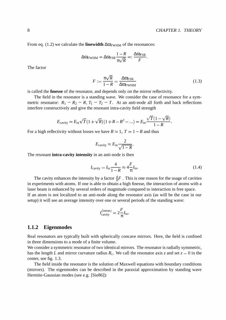
From eq. (1.2) we calculate the linewidth ∆ωFWHM of the resonances:

∆ωFWHM ∆ωFSR1 R

π

R :

∆ωFSR

F The factor

F : π

R1 R

∆ωFSR

∆ωFWHM(1.3)

is called the finesse of the resonator, and depends only on the mirror reflectivity.The field in the resonator is a standing wave. We consider the case of resonance for a sym-

metric resonator: R1 R2 R T1 T2 T . At an anti-node all forth and back reflectionsinterfere constructively and give the resonant intra-cavity field strength

Ecavity Ein

T 1

R 1 R R2 Ein

T 1

R 1 R

For a high reflectivity without losses we have R 1 T 1 R and thus

Ecavity Ein2

1 R

The resonant intra-cavity intensity in an anti-node is then

Icavity Iin4

1 R 4

Fπ

Iin (1.4)

The cavity enhances the intensity by a factor 4πF . This is one reason for the usage of cavities

in experiments with atoms. If one is able to obtain a high finesse, the interaction of atoms with alaser beam is enhanced by several orders of magnitude compared to interaction in free space.If an atom is not localized to an anti-node along the resonator axis (as will be the case in oursetup) it will see an average intensity over one or several periods of the standing wave:

Imean

cavity 2Fπ

Iin 1.1.2 Eigenmodes

Real resonators are typically built with spherically concave mirrors. Here, the field is confinedin three dimensions to a mode of a finite volume.We consider a symmetric resonator of two identical mirrors. The resonator is radially symmetric,has the length L and mirror curvature radius Rc. We call the resonator axis z and set z 0 in thecenter, see fig. 1.3.

The field inside the resonator is the solution of Maxwell equations with boundary conditions(mirrors). The eigenmodes can be described in the paraxial approximation by standing waveHermite-Gaussian modes (see e.g. [Sie86]):


2w0

z

y

x

L

Figure 1.3: Fundamental TEM00 mode.

Em n x y z t E0Xm x z Yn y z e ikz L

2 eiωt c c

Xm x z 1w z Hm 2

xw z exp x2

w2 z ikx2

2R z i2m 1

2ψ z

Yn y z 1w z Hn 2

yw z exp y2

w2 z iky2

2R z i2n 1

2ψ z

with

w0 : modewaist w z w0 1 zzR 2 : mode radius (1.5)

zR πλ

w20 : Rayleigh range

R z z z2R

z: wavefront curvature

ψ z arctan zzR : Guoy phase

Here H j x j 0 1 2 are the corresponding Hermite polynomials of the order j. The so-lutions for different m n !#" have different field distribution in radial direction and are calledTEMm n transversal modes.The boundary condition is, that on reflection the curvature radii of the wavefront and the mirror

must be equal, i.e. R L2 ! Rc. This determines the waist w0:

w20 λ

π L

2 Rc L

2 (1.6)

10 CHAPTER 1. THEORY

The most important mode is TEM00 or fundamental mode:

E0 0 x y z E01

w z exp r2

w2 z ikr2

2R z iψ z e ikz L

2 c c (1.7)

with r2 : x2 y2. This corresponds to two counter-propagating Gaussian beams. We will workwith this mode in the resonator since it has the most homogeneous radial intensity distributionwithout nodes.

Because of the Guoy phase the different transversal modes are non-degenerate. The roundtrip phase is

φn m 2Lk 2 m n 1 ψ L2 ψ L2 2π

∆ωFSRω 2 m n 1 arccos 1 L

Rc

The resonance condition is φn m ! 2πq q 1 2 . We get

ωn m ∆ωFSR q 1π m n 1 arccos 1 L

Rc (1.8)

The resonance frequencies of transversal modes are equidistant. q is the longitudinal order,i.e. the number of antinodes in the resonator. The modes with equal m n are degenerate. Themode separation depends on the length of the resonator, we will use this relation later to measurethe mirror distance of an assembled cavity.

In the experiment we often scan the mirror distance and not the laser frequency. A changeof λ

2 in the distance corresponds to ∆ωFSR. For ∆L $ λ2 % L we have ∆ω ∝ ∆L in very good

approximation.

1.1.3 Quantization of the electromagnetic field

Up to now we dealt with classical electromagnetic fields in the resonator. In order to understandthe quantum optical phenomena we need a treatment on a single photon level. The quantumfield will be used to analyze the interaction of an atom with the cavity mode. The method forintroducing photons is the canonical field quantization (see e.g. [Sho90], [Scu97]).

We consider monochromatic light of the frequency ω in the fundamental mode of the cavity.Suppose, it is linearly polarized, then there are only two mutually orthogonal components E andB of the field. The idea of the quantization is that for the standing wave fields in the resonatorthis problem has the structure of a harmonic oscillator. E plays the role of the “position” and Bis the “momentum”.

The quantum mechanical formalism expresses the field operators in terms of creation andannihilation operators a† and a:&

E x y z E00 x y z a† a &B x y z iB00 x y z a† a


where the spatial parts E00 x y z and B00 x y z are the same as in eq. (1.7).The operators a† a add and remove monochromatic, polarized photons in the resonator. The

quantum mechanical expression for the energy is&H (' ω a†a 1

2 The operator a†a counts the number of photons, ' ω is the energy of a single photon. The energyeigenstates are photon number states 0 ) 1 ) 2 ) In this picture the field in the resonator consists of photons which are reflected forth and backbetween the mirrors.

1.1.4 Photon lifetime

Since the reflectivity of the mirrors is limited, the photon will stay in the resonator only for alimited period of time. We can find it as follows:

The round trip time of the photon is ttrip 2Lc 2π

∆ωFSR. The intensity loss during half a

round-trip (one reflection) is:

I t I t 12 ttrip

12 ttrip

I t 1 Rπ

∆ωFSR

I t R∆ωFSR

F I t R∆ωFWHM I t ∆ωFWHM

Since the cavity is traversed at the velocity of light, ttrip is small and thus

I t 12ttrip I t

12ttrip

dIdt

I t ∆ωFWHM* I t I0e ∆ωFWHMt I0e tτ (1.9)

The intensity decays exponentially and

τ : 1∆ωFWHM

F∆ωFSR

(1.10)

is the photon lifetime.One defines the photon loss rate as:

κ : 1τ (1.11)

The mean number N of reflections in the cavity is given by:

N 2τ

ttrip 2

∆ωFSR

2π∆ωFW HM F

π


1.2 Atom-cavity interaction

With the basic properties of the resonator we can now analyze what happens with atoms in thecavity.

1.2.1 Atom-cavity coupling strength

To describe the atom in a way similar to the photon picture we use the second quantizationformalism. We consider a two level atom with ground and excited states g ) e ) and introducethe operators σ† : e ),+ g and σ : g ),+ e which create and annihilate atomic excitation.

Suppose the atom is placed in an antinode of the standing wave, such that the spatial depen-dence of the interaction can be omitted. The dominating part is the interaction of the atomicdipole moment with the electric field component (dipole approximation).The interaction Hamiltonian in the Heisenberg picture is&

Hint &d &E d σ†eiω0t σe iω0t E a†eiωct ae iωct

where ω0 is the atomic transition frequency, ωc is the cavity photon frequency, a† a create/annihilatecavity photons, d is the electrical dipole moment of the atom, and E is a constant which dependson the mode volume V (see [Scu97]):

E ' ωc

2ε0V

V π4

w20L λ

4L L

2 Rc L2

The expression for the mode volume is valid for L % zR.In the rotating wave approximation ω0 ωc % ω0 ωc the Hamiltonian reduces to:&

Hint dE σ†a σa† ' g σ†a σa† where

g : dE' d2ω2 ' ε0V

(1.12)

is the atom-cavity coupling rate. This interaction Hamiltonian is also known as Jaynes-CummingsHamiltonian [Jay63].

1.2.2 Jaynes-Cummings model

In the Jaynes-Cummings model we consider the interaction of a two level atom with a singlemode optical cavity. The system shall be ideal, the atom can not decay spontaneously from theexcited state to the ground state, and also photons do not escape the resonator.

1.2. ATOM-CAVITY INTERACTION 13

The full Hamiltonian including the atomic and cavity energy is given by:&H (' ω0σ†σ -' ωc a†a 1

2 -' g σ†a σa† The atom can be excited by absorbing a cavity photon or go to the ground state giving its excita-tion to the cavity. Since

σ†a σa† e n )+ g n 1 g n 1 ).+ e n the interaction couples the states g n 1 ) and e n ) for each photon number n. In the sub-manifold of these two states we can write the Hamiltonian:&

Hn '2

/01 ωc ω0 2

n 1 g2

n 1 g ωc ω0 2.34

which can be easily diagonalized giving the energy eigenvalues 5762 ωc ω0 2 4 n 1 g2.

The interaction lifts the degeneracy between the atom and the cavity. The eigenstates aresplit, see fig. 1.4, which is called vacuum Rabi splitting. In resonance, i.e. ωc ω0, thesplitting is 2

n 1 8' g. The coupled atom and cavity become one system with two resonances.

g

g

|0⟩|g |0⟩ ⟩

|1⟩

g|2⟩

( |1 +|e |g |2 )⟩ ⟩ ⟩ ⟩21

( |1 -|e |g |2 )⟩ ⟩ ⟩ ⟩21

( |0 +|e |g |1 )⟩ ⟩ ⟩ ⟩21

( |0 -|e |g |1 )⟩ ⟩ ⟩ ⟩21

2

g2

|g⟩

|e⟩

+atom cavity =

E

combined and coupledatom-cavity system

Figure 1.4: Eigenstates of the resonant atom-cavity system.


1.2.3 Dissipation and strong coupling

In the real atom-cavity system, the mirrors have a limited reflectivity and the atomic excited statehas a finite lifetime. There are 3 important processes :

1. coherent atom-photon interaction at the rate g,

2. incoherent photon leakage from the cavity at the rate κ,

3. incoherent spontaneous decay of the atomic excited state at the rate Γ.

Γ

κ g

Figure 1.5: Parameters of atom-cavity system.

The two last processes lead to loss of coherence. In a cavity QED experiment one often wantsto study or to use the coherent interaction with as little damping as possible. It means that thecoherent evolution must be fast compared to the decoherence processes. One has to get into theregime of strong coupling:

g 9 κ Γ This enables coherent energy exchange between atom and cavity within the lifetime of the atom-cavity system. For a large g the mode volume has to be small according to eq. (1.12). A lowphoton loss rate κ is achieved by a high reflectivity of the mirrors.

1.2.4 Density matrix approach

The dissipation does not only make the experiment difficult, its theoretical treatment also requiresadvanced tools. One has to consider the interaction of the system with the environment whichleads to a thermal statistical equilibrium. This can be done in the density matrix formalism.

Our atom-cavity system is now coupled to the environment. The evolution of the wholesystem including the environment can be described by a Schrodinger equation. Since the exactquantum state of the environment is not known, one traces (takes the mean value) over environ-mental states and obtains the master equation [Car93]:

ddt

&ρ 1

i ';: &H &ρ <, κ2 2aρa† a†aρ ρa†a Γ

2 2σρσ† σ†σρ ρσ†σ (1.13)


Here,

&ρ is the density matrix for the atom-cavity system, κ are cavity losses, Γ is the decay rate

of the atomic excited state. The first part of the master equation describes coherent evolution,the terms with κ and Γ are responsible for the dissipation processes which lead to decoherence.The Hamiltonian contains the atom and cavity energies, the atom-cavity interaction and coherentdriving of the cavity by a laser field of frequency ωl&

H ' ω0 ωl σ†σ -' ωc ωl a†a =' g σ†a σa† =' ε a† a In the presence of decoherence the master equation has a steady state d

dt

&ρ ! 0. This is a

system of (infinitely many) homogeneous linear equations. Numerical tools for solving the mas-ter equation exist, e.g. [Tan02]. They provide the spectra of the system and expectation valuesof atom and cavity states by restricting the dimension of the Hilbert space to a computationallyaffordable value. The structure of the solution, however, remains hidden in this approach.

My goal was to find an analytical solution of the problem in a reasonable approximation. Ihave solved the master equation analytically in the case of a weak driving field. For details seeAppendix A.

In case of resonance between atom and cavity, ωc ω0, the result is

ρ11 ε2 Γ4

2 ω2l

ω4l ( 1

4 κ2 Γ2 2g2 ω2l κΓ

4 g2 2ρ22 ε2g2

ω4l 1

4 κ2 Γ2 2g2 ω2l κΓ

4 g2 2 where ρ11 is the probability of finding a photon in the cavity and ρ22 is the population of theexcited state of the atom. The photon flux from the cavity is then κρ11. The approximationrequires that the driving laser field ε must be small, such that ρ11 ρ22 % 1.

The figure 1.6 shows the Rabi splitting in this solution. The two curves are ρ11 ωl ρ22 ωl ,i.e. the populations of cavity and atom excited states as functions of the driving laser detuningto atomic resonance. The first one is equivalent to the transmission spectrum of the cavity withan atom inside, when probed by a weak laser. The width of the lines is a sign of the presence ofdissipation.

Analysis

To connect this result to the Jaynes-Cummings model, we determine the splitting of the peaksand the linewidth of the cavity transmission. For this purpose we rewrite the expression for ρ11

into two separate peaks:

ρ11 ωl ε2

2δ α ωl ωl β 2 γ2 α ωl ωl β 2 γ2

where α β γ δ are expressions in terms of g κ Γ. The peaks are asymmetrically broadened butin the regime of strong coupling still well separated. The vacuum Rabi splitting can be found bydetermining the positions of the maxima. The approximate expression is


0

0.002

0.004

0.006

0.008

0.01

popu

latio

n

–150 –100 –50 0 50 100 150

laser detuning [MHz]

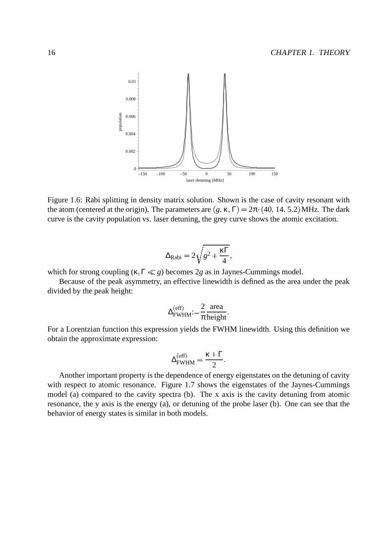
Figure 1.6: Rabi splitting in density matrix solution. Shown is the case of cavity resonant withthe atom (centered at the origin). The parameters are g κ Γ 2π 40 14 5 2 MHz. The darkcurve is the cavity population vs. laser detuning, the grey curve shows the atomic excitation.

∆Rabi 2 g2 κΓ4

which for strong coupling (κ Γ % g) becomes 2g as in Jaynes-Cummings model.Because of the peak asymmetry, an effective linewidth is defined as the area under the peak

divided by the peak height:

∆eff

FWHM: 2π

areaheight

For a Lorentzian function this expression yields the FWHM linewidth. Using this definition weobtain the approximate expression:

∆eff

FWHM κ Γ2

Another important property is the dependence of energy eigenstates on the detuning of cavitywith respect to atomic resonance. Figure 1.7 shows the eigenstates of the Jaynes-Cummingsmodel (a) compared to the cavity spectra (b). The x axis is the cavity detuning from atomicresonance, the y axis is the energy (a), or detuning of the probe laser (b). One can see that thebehavior of energy states is similar in both models.


–150

–100

–50

0

50

100

150

ener

gy [

MH

z]

–150 –100 –50 50 100 150

cavity detuning [MHz]

(a)

–150

–100

–50

50

100

150

lase

r de

tuni

ng [

MH

z]

–150 –100 –50 50 100 150

cavity detuning [MHz]

(b)

Figure 1.7: (a) Energy levels of the Jaynes-Cummings model vs. cavity detuning. (b) Cav-ity photon number of density matrix solution vs. cavity- and probe laser detuning. The whitearea corresponds to 0 photons, black area to 0 02 photons in the cavity for ε 1. The atomicresonance is centered at the origin. The parameters are g κ Γ 2π 40 14 5 2 MHz.


1.2.5 Interaction between two atoms

Two atoms which simultaneously couple to the same cavity mode become mutually coupled andcan exchange energy (information) via a cavity photon.

Suppose the atoms are at different positions within the mode and thus have in general differ-ent couplings g1 g2. The interaction Hamiltonian with the cavity is the sum of two single-atominteractions: &

Hint (' g1 σ†1a σ1a† -' g2 σ†

2a σ2a† If the cavity is tuned far from the atomic resonance, the exchange of excitation between atomand cavity becomes negligible. Two atoms can still exchange their excitation via the cavity. Theeffective second order interaction Hamiltonian is&

H2

int ' g1g2 ωc ω0 σ†1σ2 σ1σ†

2 This is a two-photon process, where one atom emits a (virtual) photon into the cavity modeand the other one absorbs it. Both processes happen simultaneously, the excited state popula-tion remains small and can be adiabatically eliminated. One gets a cavity induced atom-atominteraction.

|e,g⟩ ⟩|0 | ,g e |0⟩ ⟩

| ,g g |1⟩ ⟩

g1

g2

ω ω-0 c

Figure 1.8: Cavity which is detuned far from the atomic resonance couples two atoms via avirtual cavity excitation.

The interaction described above has a long range because the radiation is concentrated into asingle mode. For close distances between the atoms it is also possible to observe cavity amplifieddipole-dipole or van der Waals interaction (see for example [Osn01]).

This scheme is only one possibility for coupling of two atoms via the cavity. There exist dif-ferent schemes which propose to use the cavity for conditional quantum logic and entanglement(e.g. [Yi02]). The goal of future work in our group will be to implement one of those schemesto entangle two atoms.

Chapter 2

Cavity setup

The task to achieve strong coupling represents an experimental challenge. In order to performexperiments with Cs atoms, where the excited state decay rate is Γ 2π 5 2MHz, to achieveg 9 Γ we need a mode volume V $ 7 8 105 µm 3. To minimize the photon loss rate κ, the mirrorreflectivity should be as high as possible. We have set up a resonator with the goal to fulfill theserequirements. At the same time, the resonator has to be combined with our setup which deliverssingle cold Cs atoms. A suitable mechanical mounting system was built up and tested togetherwith the cavity.

2.1 Resonator assembly

The first resonator was built for testing purposes by Y. Miroshnychenko in [Mir02]. Our nexttask was to set up a new resonator which can be integrated in our setup.

2.1.1 High reflectivity mirrors

The mirrors are manufactured by the company Research Electro Optics, Boulder, USA. The highreflectivity is achieved by a stack of several ten dielectric λ > 4 layers. The specified reflectivityof the mirrors is R 99 997% for the wavelength of the Cs D2 line (852nm), corresponding to afinesse of 104000. The spherical concave surface has a diameter of 1mm and radius of curvatureof Rc 10 mm, see fig. 2.1. The special conical shape of the substrate is needed because of thelimited space in our setup as shown in sec. 2.3.4.

We have ordered a set of 30 mirrors. In [Mir02] two resonators were built showing a fi-nesse of 77000 and 94000, both below specification. This shows that a careful inspection andcharacterization of the mirrors is needed before assembling a resonator.

At this point the tools for such a characterization were quite limited. At the beginning weinspected the mirrors visually with a 100x microscope. It provides light-field and dark-field ob-servation. Using this microscope we have seen spots of different sizes on almost all mirrors.Those were ranging from macroscopic dust or glass particles down sub micrometer surface de-fects. By illuminating the surface from the side we were also able to see thin scratches on many

19

20 CHAPTER 2. CAVITY SETUP

∅3

mm

4 mm

radius of curvature:mirror surface

cR = 10 mm

∅1

mm

Figure 2.1: High reflectivity mirror, manufactured by the REO company.

mirrors. Then we used another microscope with 500x magnification which provides light-field,dark-field and better resolution. The closer look revealed more scratches and even more spots ofsub-micrometer size, one example is shown in fig. 2.2. All visible defects reduce the finesse byscattering or absorbing light.

Figure 2.2: Microscope picture of the mirror surface, 500x magnification, dark-field observation.One sees a thin scratch, one clearly visible spot on the lower left and 3 smaller spots on the upperright. The dark objects in the lower part are defects of the camera.

In order to achieve the best finesse, we looked for mirrors which were free from defects inthe center part of the mirror surface ( 0 25 mm radius). Since the TEM00 mode will have aradius of about 15 µm this should guarantee that the defects do not limit the finesse. Since allmirrors have at least several spots in the center part, we chose mirrors without scratches in thisregion. Scratches are permanent, while spots can be small dust or glass particles, thus it mightbe possible to remove them. Due to the small mirror size and sensitivity of the mirror coating,special care has to be taken when trying to clean the surface.

2.1. RESONATOR ASSEMBLY 21

We investigated the following methods for removing spots:? OptiClean: a droplet of special polymer (manufactured by Merchan Tek Inc., San Diego,USA) is placed on the surface and covered with a piece of cleaning tissue. The polymerflows over the surface as a homogeneous layer and embeds the particles. After the drying(15-20 min) the tissue is easily removed together with the polymer. Bigger particles canbe removed this way. Only a part of smaller particles is removed, several repetitions of theprocedure are needed and it does not guarantee the removal of all particles. In rare casesthe polymer can stick to the side of the mirror if too much was used, this residue has thento be removed with acetone. In general, using the polymer is fast and safe, since there isalmost no risk of damaging the surface.? mechanical cleaning: a piece of lens cleaning tissue is folded, wet in acetone and sweptwith a tweezer from the center to the border of the mirror. This method is difficult anddangerous since it is possible to produce additional scratches by dragging a piece of glassover the surface. We tried this method but decided not to use it because it had nearly noeffect on smaller spots.? bathing in acetone or methanol: the mirror is placed into warm acetone or methanol of ultrahigh purity. After about 5 minutes the mirror is taken out holding the surface vertical suchthat no liquid drop can stay on the surface. If some liquid would dry out on the surface, itwould leave the dissolved dirt behind. This method is able to remove some of the spots,even small ones, but it can also add spots on some cases. It also removes the residue of theOptiClean polymer which could stick to the side of the mirror and cause problems with theultra high vacuum needed in the experiment.? ultrasonic bath: the mirror is placed into a small vessel filled with pure acetone and put intoan ultrasonic bath for about 5 min. This device is filled with water and produces ultrasonicvibrations of the liquid which remove particles from the surface. However particles canproduce scratches. Small spots are not removed.

After considering all methods we decided to clean selected mirrors by applying OptiClean severaltimes and then doing both an acetone and a methanol bath. The surfaces were inspected aftercleaning with the 500x microscope and the procedure was repeated when necessary. By thesemeans we were able to find a mirror pair with no visible scratches and almost no spots in thecenter region of the surface.

2.1.2 Assembly

Piezo elements

For precise control of the resonator length the mirrors are glued onto piezo elements. We useshear piezos (PI Ceramic, 6x6x1 mm), which perform a shear movement of 5 300 nm when avoltage of 5 500 V is applied. This is enough to scan over a free spectral range of λ

2 426 nmeven when only one piezo is used.


Holder

The holder for the mirrors is designed for precise positioning of the cavity in our setup. It isdescribed in all detail in sec. 2.3.4.

The procedure of assembly is almost the same as described in the diploma thesis [Mir02].First, the piezo elements are glued onto the holder. The holder also provides electric groundcontact. Before gluing, the mirrors are fixed to the piezo surfaces with a positioning tool whichaligns them coaxially in a V-groove, see fig. 2.3. This ensures that the mode is well centered tothe axis of both mirrors.

The next step is gluing of the mirrors to the piezo elements. The previous method was to put aglue droplet under the mirror, where it distributes as a thin layer. The problem of this approach isthat the glued surface is big. When the glue cures it can contract introducing mechanical tensionto the mirror substrate. This tension leads to a birefringence and should be avoided. The generalrule is to reduce the contact area of the glue, presumably to only one or two points. The ideais to put the glue not directly between the mirror and the piezo but rather to use an additionalglass cylinder (glass fiber) of few hundred micrometer diameter lying parallel to the mirror side.It is glued with one side to the piezo and with the other side to the mirror (see figure). Usingthe cylinder has also an additional advantage that it might be possible to remove a glued mirror.When glued directly, the removal destroys the mirror and the piezo, because of the large contactarea with the glue. Figure 2.4 shows the assembled cavity on the holder.

cavity holder

shear piezo

glue

mirror

positioning tool

view fromabove

glass cylinder(optional)

V-groove

side view

Figure 2.3: Assembly of the cavity.

2.2. CHARACTERIZATION OF THE CAVITY 23

Figure 2.4: Assembled cavity in the glass cell of the test vacuum setup.

2.2 Characterization of the cavity

The most important parameters of the resonator are its length and the linewidth. Knowing themone can calculate the values of g and κ which are important for future cavity QED experiments.

Cavity test setup

For characterization and testing purposes the cavity was placed inside a vacuum chamber whichis geometrically identical to the vacuum chamber of the main experiment. By doing so we areable to test the interplay of the cavity holder with the chamber geometry. This is important forlater integration of the resonator into the main setup, for details see section 2.3.4. The opticalpart of the setup is shown in fig. 2.5.

There are two lasers in the setup, the probe laser (852 nm) and the lock laser (836 nm). Theprobe laser is resonant with the Cs atom, the second is used for cavity stabilization as describedin the next chapter. Both lasers are delivered by the same fiber in orthogonal polarizations and arethus perfectly overlapped which reduces the amount of work for coupling them into the cavity.

The laser beams pass a specially designed mode matching telescope (see [Mir02], p. 23)which tailors their waist to match the fundamental TEM00 cavity mode. The geometrical cou-pling into the cavity mode is done with two mirrors. The transmitted light is imaged onto a CCDcamera, which enables us to distinguish transversal modes. The transmitted power is measuredwith a photo-multiplier (Hamamatsu H7712-03). In order to reduce the straylight, a 200 µmpinhole is placed in front of the detector.

The reflected beam passes back through the telescope, is coupled out with an unpolarizingbeam-splitter and is focussed onto a fast photodiode (Newport amplified silicon PIN, 818-BB-21A). Its signal is used for the Pound-Drever-Hall stabilization of the QED cavity.

The voltage for the piezo elements is a triangle scan with variable amplitude and offset, which


glass cell

HV

CCDcamera

photodiode:

probe laser,lock laser

mode m

atchingtelescope

incident beam

reflected beam

fast PDfor locking

transmission

observationlens

pinhole

cavity

Figure 2.5: Optical setup for characterization and stabilization of the cavity.

is amplified to the necessary high voltage ( 5 400V) by a low noise amplifier (FLC Electronics,A800-40).

Mode matching

In order to achieve the coupling of the laser into the fundamental cavity mode it is necessaryto adjust the focus and the geometrical position of the beam to match the mode. The piezosare scanned at an amplitude of about 100 V at 10 Hz. The incidence position and angle of thebeam are changed with a mirror and one tries to see some transmission on the camera. Thelaser can be approximately adjusted to the center of the cavity mirror. If no transmission isseen, the voltage offset for the piezo is changed and the procedure is repeated. If at least onehigher transversal mode is visible, one can look in its vicinity for the neighboring lower modeby slightly changing the coupling angle. For identifying the individual transversal modes, thescan amplitude is reduced. By these means one moves down to the fundamental mode which is


then optimized with both mirrors. A coupling efficiency of 50% in the fundamental mode can beusually reached without additional effort. For a better coupling one can also adjust the telescopewith and change its focus.

2.2.1 Voltage-travel relation of piezo elements

For precise control of the cavity resonance frequency one has to know precisely how the piezo el-ements change the resonator length with applied voltage. Their voltage-travel correspondence isin general nonlinear, given by the properties of the piezo material. As we know from eq. (1.8) thetransversal modes of the resonator are equidistant and thus define a frequency scale. Therefore,we can measure the voltages corresponding to resonance of different transversal modes.

In order to get some intensity into the higher transversal modes, the coupling of the laserinto the cavity was slightly misaligned. The piezo voltage was scanned slowly (1 Hz) over themaximal range ( 5 400 V) and the transmission peaks were recorded.

The transmission curve is shown in the figure 2.6, (a). It shows two free spectral ranges ofthe resonator. One can identify a large number of clearly visible transversal modes and assignthem corresponding frequencies (transversal mode numbers). Due to the large scan range, thetime during which the intensity of each mode is recorded is small, resulting in strong variationsof the peak height.

The resulting response curve is shown in 2.6, (b). The displacement is slightly non-linearand depends quadratically on the voltage within this scan range. Additionally it has a hystere-sis feature. Another important parameter is the voltage distance of two neighboring transversalmodes for a small scan range (i.e. of the order of the mode separation itself). This distance wasmeasured to be constant, its slope is shown in the curve. This is an important result, since thevoltage-frequency relation is then linear and constant for small scan ranges used in the experi-ment or for stabilization.

2.2.2 Resonator length

The control of the mirror distance during the assembly process is not very precise. The finaldistance is only known after the assembly is finished. It can, however, be deduced with highprecision from the free spectral range or the frequency distance between transversal modes. Thelatter alternative is easier to measure since the transversal mode distance is small and thus stillin the linear range of the piezo response. One problem is that the correspondence between thevoltage scan and the frequency is unknown at this point. To get the absolute scale of frequencythe laser beam is modulated by an AOM which produces a sideband at a defined distance fromthe main line, see fig. 2.7.

The procedure of measuring the distance between transversal modes is the following: bothpiezo elements are scanned in parallel at about 50 Hz, the scan amplitude is adjusted to be justabove the spacing between neighboring modes. Then the mode distance is measured, togetherwith the AOM sideband distance. Setting both values in relation one gets the result in frequencyunits. We measured the following value:


(a)

(b)

Figure 2.6: Measurement of the voltage-travel relation of the piezo elements. Figure (a) showsthe transmission of transversal modes vs. mirror scan, figure (b) shows the response curve. They-axis in (b) is proportional to the resonator length changes. For a small scan range between twoneighboring modes one obtains a different response, which is also shown.


TEM01

TEM00

tran

smis

sion

AOMsideband

cavity length scan

∆ωtrans

Figure 2.7: Measurement of the transversal mode distance (schematic). One sees the transmis-sion of two neighboring transversal modes and the AOM sidebands.

∆ωtrans 2π 70 38 GHz The error of this measurement is due to the limited resolution of the oscilloscope. It is of the orderof 1 2%. A possible systematic error might be caused by the non-linearity of the piezo elementsat the small scan range. This effect could not be measured, since there are no transmission linesbetween the neighboring transversal modes.In order to calculate the cavity length L we use eq. (1.8) to get

∆ωtrans 1π

∆ωFSR arccos 1 LRc c

Larccos 1 L

Rc

This transcendent equation is solved numerically for L. The resulting cavity length is:

L 92 2 µm and the free spectral range is ∆ωFSR 2π 1 63 THz.The obtained value L is the effective cavity length. Since the mirror surface is a stack of dielectriclayers, the light penetrates about 2µm into the mirror, thus the physical mirror distance is slightlyshorter.

2.2.3 Cavity linewidth and finesse

In order to obtain the photon loss rate κ and finesse F , we have to determine the spectral linewidthof the cavity. The cavity is scanned over the resonance of the TEM00 mode and the AOM side-band, see fig. 2.8. Similar to the previous measurement, the FWHM linewidth is compared tothe distance of the AOM sideband. Knowing the AOM frequency, we directly get the linewidth.

The main difficulty of this measurement is the required stability of the resonator. All kinds ofmechanical (acoustical) and electronical noise make the line move, fluctuate or change its shape.


Figure 2.8: Cavity transmission showing the TEM00 line and its AOM sideband, averaged over64 measurements.

Parts of the equipment, especially those which produce vibrations (e.g. vacuum pumps), have tobe switched off.We obtained the following values:

κ ∆ωFWHM 2π 13 77 MHz F ∆ωFSR

∆ωFWHM 118000

The errors produced by the reading of the instrument are again 1 2%. The environmental noise,however, has a substantial impact on the linewidth. Performing this measurement in a somewhatnoisier situation we obtained a larger linewidth of about 16 MHz.

The finesse is just above the specification of the manufacturer (Fspec 104000) and is higherthan the finesse achieved by the previous resonators (F 77000 94000 66000). The shift of theresonance frequency of ∆ωFSR corresponds to a resonator length change of only λ

2 1F 3 6 pm,

thus the length stability becomes an important issue.

2.2.4 Resulting parameters

Knowing the mirror distance of L 92 µm we can calculate the waist w0 and the coupling pa-rameter g.

According to eq. (1.6) : w20 λ

π @ L2 Rc L

2 . For λ 852 nm L 92 µm Rc 10 mm weget

2.3. SINGLE-ATOMS SETUP 29

w0 13 5 µm The mode volume is V π

4 w20L for our parameters we get

V 1 3 104 µm 3 Finally we calculate the coupling parameter according to eq. (1.12):

g d2ω2 ' ε0V

using the values (see [Ste98]):d 2 698 10 29 Cm ω 2π 351 7 THz we obtain

g 2π 40 3 MHz Altogether we have: g κ Γ 2π 40 3 13 8 5 2 MHz i.e.

g2

κΓ 22 6

which indicates that we should be able to achieve the strong coupling regime.

2.3 Single-atoms setup

Our main experimental setup allows us to deterministically deliver single cold Cs atoms to adefined position [Kuhr01]. Furthermore it is capable of preparation, coherent manipulation andmeasurement of the atomic hyperfine states, see [Kuhr03].

2.3.1 Single-atom MOT

Our source of single cold Cs atoms is a magneto-optical trap (MOT). It consists of three pairs ofcounter-propagating red detuned laser beams which constitute a so called optical molasses. Theatoms from the dilute background Cs gas are Doppler cooled to a temperature of about 100 µK.A high-gradient magnetic quadrupole field creates position dependent Zeeman splitting of theatomic hyperfine sub-levels. Together with the circular polarization of the beams this gives theposition dependent restoring force needed for trapping. Details of the MOT are described in[Kuhr03]. The fluorescence light of the atoms in the trap is monitored by an avalanche photodi-ode. This enables us to count the exact number of atoms.


vacuum chamber

MOT

MOT laser beams

glasscell

magneticcoils

APD

intensifiedCCD

dipole trap laser

Cs

MWantenna

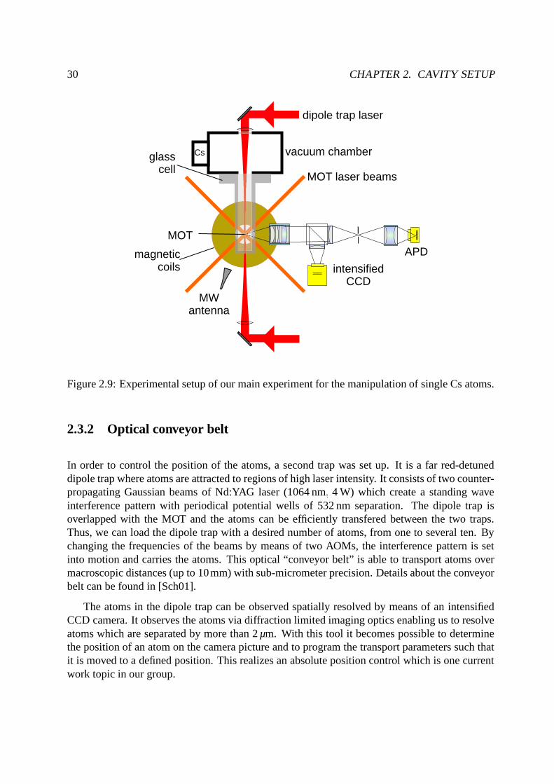
Figure 2.9: Experimental setup of our main experiment for the manipulation of single Cs atoms.

2.3.2 Optical conveyor belt

In order to control the position of the atoms, a second trap was set up. It is a far red-detuneddipole trap where atoms are attracted to regions of high laser intensity. It consists of two counter-propagating Gaussian beams of Nd:YAG laser (1064 nm 4 W) which create a standing waveinterference pattern with periodical potential wells of 532 nm separation. The dipole trap isoverlapped with the MOT and the atoms can be efficiently transfered between the two traps.Thus, we can load the dipole trap with a desired number of atoms, from one to several ten. Bychanging the frequencies of the beams by means of two AOMs, the interference pattern is setinto motion and carries the atoms. This optical “conveyor belt” is able to transport atoms overmacroscopic distances (up to 10mm) with sub-micrometer precision. Details about the conveyorbelt can be found in [Sch01].

The atoms in the dipole trap can be observed spatially resolved by means of an intensifiedCCD camera. It observes the atoms via diffraction limited imaging optics enabling us to resolveatoms which are separated by more than 2 µm. With this tool it becomes possible to determinethe position of an atom on the camera picture and to program the transport parameters such thatit is moved to a defined position. This realizes an absolute position control which is one currentwork topic in our group.


2.3.3 Manipulation and measurement of internal states

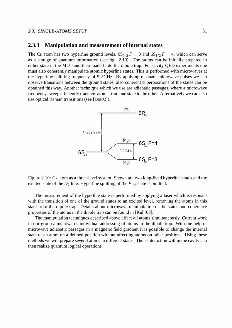
The Cs atom has two hyperfine ground levels, 6S1 A 2 F 3 and 6S1 A 2 F 4, which can serveas a storage of quantum information (see fig. 2.10). The atoms can be initially prepared ineither state in the MOT and then loaded into the dipole trap. For cavity QED experiments onemust also coherently manipulate atomic hyperfine states. This is performed with microwaves atthe hyperfine splitting frequency of 9 2GHz. By applying resonant microwave pulses we canobserve transitions between the ground states, also coherent superpositions of the states can beobtained this way. Another technique which we use are adiabatic passages, where a microwavefrequency sweep efficiently transfers atoms from one state to the other. Alternatively we can alsouse optical Raman transitions (see [Dot02]).

|e⟩

|g ⟩1

|g ⟩2

6S F=31/2

6S F=41/2

6P1/2

6S1/2

λ=852.3 nm

9.2 GHz

Figure 2.10: Cs atom as a three-level system. Shown are two long-lived hyperfine states and theexcited state of the D2 line. Hyperfine splitting of the P1 A 2 state is omitted.

The measurement of the hyperfine state is performed by applying a laser which is resonantwith the transition of one of the ground states to an excited level, removing the atoms in thisstate from the dipole trap. Details about microwave manipulation of the states and coherenceproperties of the atoms in the dipole trap can be found in [Kuhr03].

The manipulation techniques described above affect all atoms simultaneously. Current workin our group aims towards individual addressing of atoms in the dipole trap. With the help ofmicrowave adiabatic passages in a magnetic field gradient it is possible to change the internalstate of an atom on a defined position without affecting atoms on other positions. Using thesemethods we will prepare several atoms in different states. Their interaction within the cavity canthen realize quantum logical operations.


2.3.4 Integration of the cavity into current setup

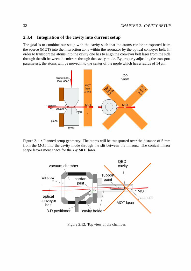
The goal is to combine our setup with the cavity such that the atoms can be transported fromthe source (MOT) into the interaction zone within the resonator by the optical conveyor belt. Inorder to transport the atoms into the cavity one has to align the conveyor belt laser from the sidethrough the slit between the mirrors through the cavity mode. By properly adjusting the transportparameters, the atoms will be moved into the center of the mode which has a radius of 14 µm.

5 mm

MOT

probe laser,lock laser

conveyorbelt 100µm

MOT

cavity

piezo

MOTlaserz-axis

topview

MOT

laser

x-ax

is

MOTlaser

y-axis

Figure 2.11: Planned setup geometry. The atoms will be transported over the distance of 5 mmfrom the MOT into the cavity mode through the slit between the mirrors. The conical mirrorshape leaves more space for the x-y MOT laser.

3-D positioner

opticalconveyor

belt

glass cell

cavity holder

QEDcavity

MOT

vacuum chamber

MOT laser

supportpointcardan

jointwindow

Figure 2.12: Top view of the chamber.


The integration shall follow the tactics of minimal invasion, i.e. the cavity has to be added intothe setup without changing or disturbing the other parts. We aim a distance of 5 mm between theMOT center and the cavity center. The transportation has an efficiency over 80% for this distanceand the conically shaped mirrors will not block the MOT lasers, see fig. 2.11.

The position of the MOT within the setup is fixed by the magnetic field zero and can not bechanged. The position and direction of the optical conveyor belt also can not be changed withoutmuch effort. Thus the cavity has to be placed in the glass cell leaving the ability to change itsposition with high precision.

For these means the cavity is assembled on a specially designed holder. Its task is to transferthe movement of a precision 3D motional vacuum feed-through to the cavity. This positioningunit is controlled from outside the vacuum chamber giving the possibility to adjust the cavityposition. The geometry is shown in fig. 2.12. The handling of the cavity with the holder isrelatively tricky because of limited space in the vacuum chamber and the glass cell. Still, this isthe only possibility to integrate the resonator without rebuilding the whole experiment. Figure2.4 shows the cavity in the glass cell.

3Dpositioner

base(fixed)

support(movable)

cavity

cardanjoint

top view

side view

base

Figure 2.13: Kinematics of the cavity holder.

The holder consists of two parts which are connected by a cardan joint (see fig. 2.13). Thepart which holds the cavity rests on a support in the glass cell, the other part is attached to the 3Dpositioner. The support has the possibility to move along the base which is fixed in the glass cell.The 2 axes of movement of the positioner which are orthogonal to the cell axis are translated


around the support point by 1:5. The movement along the axis together with the support istranslated 1:1.

The specified precision of the 3D positioner (Thermionics Northwest XY-B450/T275-1.39precision XY manipulator + FLMM133 precision Z feed-through) is 10 µm. Thus the positionof the cavity with respect to the MOT should be adjustable with precision of 10 µm along thecell axis and with a precision of 2 µm along the two other axes. To avoid eventual contact of theholder with the walls of the chamber or glass cell which might lead to jamming and damage, thepositioner features a customizable travel limit. We were able to test the function of the holder andpositioning of the cavity. The cavity could be moved along all three axes and fixed to a definedposition.

The alignment of the dipole trap beam through the slit between the mirrors is a critical point.Since the mirrors are curved, the slit is smaller than the measured effective resonator length L.Knowing the mirror surface radius r and the radius of curvature Rc (see fig. 2.1) one can calculateits size dslit:

dslit L 2 Rc @ R2c r2 L r2

Rc

For r 0 5 mm, Rc 10 mm, the slit is 25 µm smaller than the resonator. For L 92 µm itssize is dslit 67 µm. The dipole trap laser has currently the waist diameter of 2w0 40 µm,with the focus in the center of the cavity the beam size on the slit is then about 42 µm. Firstmeasurements showed that about 95% of the power of the beam can be put through the cavityslit and glass windows in the test chamber. The power absorbed by mirror edges causes a strongthermal expansion of the mirrors which makes the spectral lines shift by a distance of severaltransversal modes when the laser is switched on. This has to be further examined and optimized.

2.4 Conclusion

We have set up and characterized a cavity with a length L 92 µm and a finesse F 118000.The cavity was assembled on a holder which enables its integration into our main experimentalsetup.

To achieve the best performance in cavity QED experiments the g2

κΓ parameter has to bemaximal. The current resonator with g κ Γ 2π 40 3 13 8 5 2 MHz has the ability toachieve the strong coupling regime. To further improve the performance, one has to increase thecoupling g and to decrease the photon loss rate κ. As we have seen in the previous section thehigh power conveyor belt laser has to fit through the slit between the mirrors and thus sets a lowerboundary to the mirror distance. The current slit size of dslit 67 µm already causes problemswith power absorbed by the mirrors. Thus the coupling rate g can not be increased. The onlyparameter which can be improved is κ, by increasing the mirror reflectivity. In this respect aquick and reliable method of characterizing mirrors before could be useful. Such a method willbe presented in chapter 4.

Chapter 3

Active stabilization of the cavity

Cavity QED experiments require precise control of the cavity resonance frequency with respectto an atomic transition. This requires a very high mechanical stability of the resonator, since dueto high finesse, fluctuations of the cavity length shift the resonance frequency by more than itswidth. The fluctuations are caused by thermal drifts and inevitable mechanical vibrations. Thepassive mechanical stability is not sufficient, an active feedback scheme is required to compen-sate for the fluctuations. In this chapter a scheme is presented which is capable of stabilizing thecavity length to a fraction of a picometer.

Active stabilization implies the use of a stable reference frequency (e.g. that of a laser). Aservo loop then holds the cavity resonant with the laser thus stabilizing its resonance frequencyto the laser frequency. In order to achieve this, an error signal must be extracted. This signalcontains the information about magnitude and sign of deviation of the resonance frequency fromthe desired value. After suitable filtering and amplification the signal is fed back to the cavity. Inour setup the extraction of the error signal is accomplished using the Pound-Drever-Hall method[Dre83].

3.1 Pound-Drever-Hall method

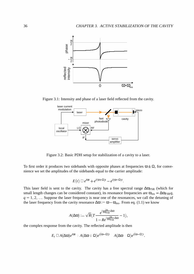
The basic idea of this method is to use the property of the laser beam reflected from the cavity toderive an error signal, see fig. 3.1. The phase of this reflection is dispersive, i.e. it changes signaround resonance. When the laser frequency matches the cavity resonance, the phase is zero; forsmall deviations it is proportional to the difference of the laser and cavity resonance frequencies.This property is used for an error signal, which can then be used to stabilize a cavity to a stablelaser, or vice versa.

The PDH method extracts the relative phase of three different frequencies which will experi-ence different phase changes. A PDH setup for stabilizing a cavity to a stable reference laser isshown in fig.3.2. The laser frequency ω is modulated with the frequency Ω, generated by a localoscillator. The field amplitude of the modulated laser beam is then:

E t ∝ exp i ω αsin Ωt t 35

36 CHAPTER 3. ACTIVE STABILIZATION OF THE CAVITY

refle

cted

inte

nsity

phas

e

π2

π2

ω ω- res0

Figure 3.1: Intensity and phase of a laser field reflected from the cavity.

laser

laser currentmodulation

fastphotodiode

cavity

LO

IF

RF

mixer

localoscillator

piezo

servoamplifier

Figure 3.2: Basic PDH setup for stabilization of a cavity to a laser.

To first order it produces two sidebands with opposite phases at frequencies ω 5 Ω, for conve-nience we set the amplitudes of the sidebands equal to the carrier amplitude:

E t ∝ eiωt eiω B Ω t ei

ω Ω t

This laser field is sent to the cavity. The cavity has a free spectral range ∆ωFSR (which forsmall length changes can be considered constant), its resonance frequencies are ωres ∆ωFSRq,q 1 2 . Suppose the laser frequency is near one of the resonances, we call the detuning ofthe laser frequency from the cavity resonance ∆ω : ω ωres. From eq. (1.1) we know

A ∆ω : R T e

i 2π∆ωFSR

∆ω

1 Rei 2π

∆ωFSR∆ω

1 the complex response from the cavity. The reflected amplitude is then

Er ∝ A ∆ω eiωt A ∆ω Ω eiω B Ω t A ∆ω Ω ei

ω Ω t

3.1. POUND-DREVER-HALL METHOD 37

The resulting intensity is measured by a fast photo-detector:

Ir ∝ Er E Cr ∝ A ∆ω D 2 A ∆ω Ω D 2 A ∆ω Ω D 2 : A ∆ω A C ∆ω Ω e iΩt A ∆ω A C ∆ω Ω eiΩt A ∆ω Ω A C ∆ω Ω ei2Ωt <, c c For phase detection, this signal is multiplied by the modulation frequency ei

Ωt B γ , where γ is

the phase of the local oscillator relative to the photodiode signal. The non-oscillating componentsof the result are: Ire

iΩt B γ DC ∝ eiγ A ∆ω A C ∆ω Ω A C ∆ω A ∆ω Ω eiγR T e

i 2π∆ωFSR

∆ω

1 Rei 2π

∆ωFSR∆ω

1 T e i 2π

∆ωFSR

∆ω B Ω

1 Re i 2π

∆ωFSR

∆ω B Ω 1

eiγR T e i 2π

∆ωFSR∆ω

1 Re i 2π

∆ωFSR∆ω

1 T ei 2π

∆ωFSR

∆ω Ω

1 Rei 2π

∆ωFSR

∆ω Ω 1

–1

–0.5

0.5

1

PDH

sig

nal

–1e+09 –5e+08 5e+08 1e+09delta omega

–1

–0.5

0

0.5

1

PDH

sig

nal

–1e+09 –5e+08 5e+08 1e+09delta omega

Figure 3.3: Real part of PDH signal for γ 0 99 π (left) and γ 12 π (right) vs. the relative

detuning ∆ω The real part of the resulting signal is shown in the figure 3.3. Around ∆ω 0 it has a

dispersive feature which we want for the error signal. Its shape depends on the phase γ which isin experiment determined by the path length of the signals from the generator and photodiode tothe mixer (multiplier). The steepest slope is obtained for γ π

2 ; γ can be adjusted by varying thecable length from the local oscillator to the mixer.

The resulting error signal can be used for stabilization. After necessary amplification it isapplied to the cavity piezo, closing the feedback loop. This loop (lock) stabilizes the resonancefrequency of the cavity to the laser frequency. Since the signal depends only on the difference of


the laser and cavity frequencies, one can use it as well for stabilizing the laser frequency to theresonance of a stable cavity.

For the case γ π2 we are interested in the steepness of the slope. For ∆ω % Ω and small

cavity linewidth (high finesse) the sidebands are far from the cavity resonance and thus

e E i 2π∆ωFSR

∆ω F Ω

1 Re E i 2π∆ωFSR

∆ω F Ω ;G 0

Furthermore we note that for ∆ω near 0 one obtains in the first order

TeF i 2π

∆ωFSR∆ω

1 ReF i 2π

∆ωFSR∆ω

T 1 5 2π∆ωFSR

∆ω 1 R 2 5 R2π

∆ωFSR∆ω

Setting T 1 R for the case of no losses, the linear part of the signal near resonance is

PDH ∆ω % Ω 4∆ω

∆ωFWHM (3.1)

As expected, the sensitivity of the error signal increases with decreasing linewidth. This meansthat a high finesse cavity produces a more sensitive error signal and can be stabilized moreaccurately.

3.2 Stabilization setup

For the application of the PDH method for cavity stabilization a stable reference laser is required.One possibility would be to use the laser at 852 nm, which is stabilized to a atomic resonance.But the presence of such a laser within the cavity would continuously excite the atom and thusdisturb its interaction with the cavity mode. Continuous stabilization requires a far detuned locklaser at low intensity which interacts only weakly with the atoms inside the cavity.

Therefore a stable laser is required which is far detuned from the 852 nm Cs resonance. Inorder to provide accurate stabilization, the mirrors should still have a high finesse for this laser,see eq. (3.1). This limits the possible detuning to few tens of nm. There is no simple methodof stabilizing the laser to an atomic resonance in this wavelength range (e.g. Rb D1 794 nm isalready too far away). Our way to solve this problem is to take a laser at 836nm and to stabilize itto the stable resonant 852 nm laser via an additional (transfer) cavity. This solution incorporatesa “chain” of 3 locks.

The figure 3.4 shows a simplified scheme of the lock chain. It begins with the resonant“probe” laser which is already stabilized to the atomic transition by means of polarization spec-troscopy and serves as a stable reference for the lock chain.

In the first step the probe laser stabilizes the transfer cavity. The laser is phase modulatedwith an EOM at 20 MHz and its reflection off the cavity is detected with PD1.

The second step is the stabilization of the lock laser. The sidebands are produced by a directmodulation of the laser diode current at 86MHz. The reflection of the lock laser from the transfer

3.3. IMPROVEMENT OF THE STABILIZATION SYSTEM 39

length: 1.23 mfinesse: 250

lock-laser

836 nm

laser currentmodulation 86 MHz

PD 2

AOM

PD 1transfer cavity

QED cavity laserPZT

probe-laser

852 nmEOM

20 MHzmodulation

AOM

resonancematching

detuning

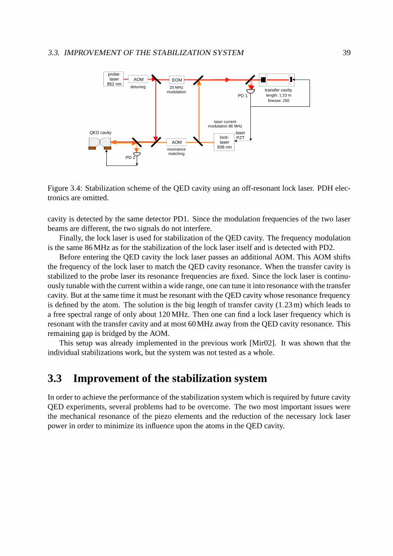
Figure 3.4: Stabilization scheme of the QED cavity using an off-resonant lock laser. PDH elec-tronics are omitted.

cavity is detected by the same detector PD1. Since the modulation frequencies of the two laserbeams are different, the two signals do not interfere.

Finally, the lock laser is used for stabilization of the QED cavity. The frequency modulationis the same 86 MHz as for the stabilization of the lock laser itself and is detected with PD2.

Before entering the QED cavity the lock laser passes an additional AOM. This AOM shiftsthe frequency of the lock laser to match the QED cavity resonance. When the transfer cavity isstabilized to the probe laser its resonance frequencies are fixed. Since the lock laser is continu-ously tunable with the current within a wide range, one can tune it into resonance with the transfercavity. But at the same time it must be resonant with the QED cavity whose resonance frequencyis defined by the atom. The solution is the big length of transfer cavity (1 23 m) which leads toa free spectral range of only about 120 MHz. Then one can find a lock laser frequency which isresonant with the transfer cavity and at most 60MHz away from the QED cavity resonance. Thisremaining gap is bridged by the AOM.

This setup was already implemented in the previous work [Mir02]. It was shown that theindividual stabilizations work, but the system was not tested as a whole.

3.3 Improvement of the stabilization system

In order to achieve the performance of the stabilization system which is required by future cavityQED experiments, several problems had to be overcome. The two most important issues werethe mechanical resonance of the piezo elements and the reduction of the necessary lock laserpower in order to minimize its influence upon the atoms in the QED cavity.


3.3.1 Compensation of resonances

Resonances in the response of a feedback loop can be either electronical (between some parasiticcapacitances and inductivities) or mechanical. At a resonance the gain profile of the feedbackloop has a π phase jump, which causes oscillations of the loop. Additionally, any driving (includ-ing noise) at the resonance frequency is enhanced by a large factor. We encountered a significantmechanical resonance of the piezo elements at a frequency of 40 kHz.

diodelaser

670 nm

QED cavity

network Analyzer

amplifier

PD

freq. sweepcavity scan

tran

smis

sion

offset

fringes

offset

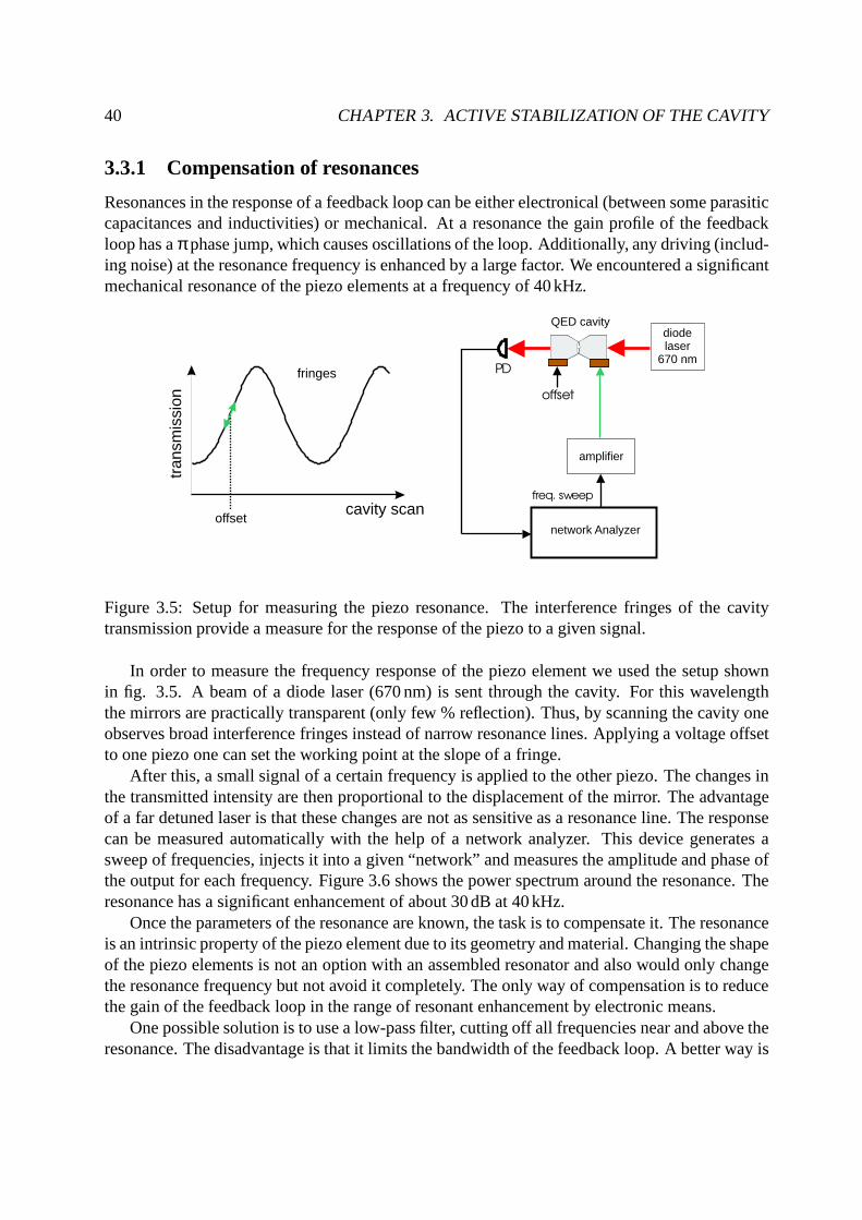
Figure 3.5: Setup for measuring the piezo resonance. The interference fringes of the cavitytransmission provide a measure for the response of the piezo to a given signal.

In order to measure the frequency response of the piezo element we used the setup shownin fig. 3.5. A beam of a diode laser (670 nm) is sent through the cavity. For this wavelengththe mirrors are practically transparent (only few % reflection). Thus, by scanning the cavity oneobserves broad interference fringes instead of narrow resonance lines. Applying a voltage offsetto one piezo one can set the working point at the slope of a fringe.

After this, a small signal of a certain frequency is applied to the other piezo. The changes inthe transmitted intensity are then proportional to the displacement of the mirror. The advantageof a far detuned laser is that these changes are not as sensitive as a resonance line. The responsecan be measured automatically with the help of a network analyzer. This device generates asweep of frequencies, injects it into a given “network” and measures the amplitude and phase ofthe output for each frequency. Figure 3.6 shows the power spectrum around the resonance. Theresonance has a significant enhancement of about 30 dB at 40 kHz.

Once the parameters of the resonance are known, the task is to compensate it. The resonanceis an intrinsic property of the piezo element due to its geometry and material. Changing the shapeof the piezo elements is not an option with an assembled resonator and also would only changethe resonance frequency but not avoid it completely. The only way of compensation is to reducethe gain of the feedback loop in the range of resonant enhancement by electronic means.

One possible solution is to use a low-pass filter, cutting off all frequencies near and above theresonance. The disadvantage is that it limits the bandwidth of the feedback loop. A better way is

3.3. IMPROVEMENT OF THE STABILIZATION SYSTEM 41

Figure 3.6: Resonance of the piezo element. The upper curve shows the response of the piezo.The lower curve shows the response compensated with a notch filter.

the use of a so called notch filter. This filter blocks frequencies only within a certain range. Weuse a simple passive design shown in the figure 3.7.

out

R

L, R

C

L

gnd

in

20 30 40 50 60-45

-40

-35

-30

-25

-20

-15

-10

-5

0

resp

onse

[dB

m]

frequency [kHz]

Figure 3.7: Schematic of a notch filter and calculated frequency response for the parameter setR 470 Ω, L 1 mH C 16 3 nF RL 4 Ω

The idea is to use a series LC circuit, where the resonance of the coil and capacitor makestheir joint resistance go to zero for a defined frequency ωres. The condition for the resonance is

iωresL iωresC

! 0 * ωres 1LC

The residual resistance is given by the ohmic resistance RL of the coil. It determines the resonant


damping factor and the width of the resonance. The damping is given by:

Uout ω ωres Uout ω 0 RL

R Inserting the filter after the high voltage amplifier before the piezo element removes all 40 kHzsignals, including noise of the amplifier. We have chosen the parameters:

R 470 Ω L 1 mH C 16 3 nF The coil has an intrinsic resistance of RL 4 Ω. Figure 3.6 shows the response with the notchfilter; the resonance is very well compensated.

To reduce minor electronical resonances we have added a resistor (10 kΩ) in series with thepiezo element. Its purpose is to damp the resonances of the piezo capacitance and inductivitiesin the amplifier and cables. These resonances usually have high frequencies, but still influencethe feedback. The resistor reduces their Q factors making the gain profile of the feedback loopsmoother. The complete loop is shown in the fig. 3.8.

locklaser

836 nm

QED cavity

HVamplifier

notch-filter

R

res.APD

PDH

servoamplifier

Figure 3.8: QED cavity lock with resonance compensation.

3.3.2 Resonantly amplified APD

The laser stabilization of the QED cavity must operate without disturbing the actual experiment.This limits the maximal power of the lock laser which can be present within the cavity beforeits influence upon the atoms becomes significant despite its detuning. One criterion is that atomsshould not scatter more photons of the lock laser than of the dipole trap laser (which is inevitablefor transporting the atoms into the cavity). The detuning ∆ of the lock laser (836 nm) fromthe atomic resonance (852 nm) is 13 times smaller than the detuning of the dipole trap laser(1064 nm). The scattering rate Γsc 1

∆2 gains a factor of 169. Additionally, the intensity of

the lock laser is enhanced within the cavity by the factor 2πF , see eq. (1.4). To be sure that the

scattering criterion is fulfilled even for a finesse of F 500000, the lock laser power must be

3.4. PERFORMANCE OF THE STABILIZATION SYSTEM 43

about 5 107 times smaller than the power of the dipole trap. For a 4 W dipole trap, the limit is80 nW. This requires a sensitive detector with a high signal-to-noise ratio.

We decided to use a resonantly amplified APD. This is an avalanche photo-detector withfrequency selective amplification. The output signal of the detector is sent to an LC circuitwhich is tailored to be resonant with the Pound-Drever-Hall modulation frequency of 86 MHz.This makes the detector sensitive especially to this frequency, and at the same time suppressesall other signal sources at other frequencies, especially noise.

The performance of the home-built resonant APD prototype was compared to the previouslyused commercial photo-detector (Newport amplified silicon PIN, 818-BB-21A). With a 400 nWlaser power the commercial photo-detector produces an error signal with a signal-to-noise ratioof 1. The stabilization worked insufficiently under such conditions.

The resonant APD, however, is able to perform a lock with less than 200 nW coupled intothe fundamental mode of the cavity and less than 100 nW at the detector. The final version ofthe detector will have an improved electronics part and it will also use a photodiode with bettercharacteristics. With these improvements it will fulfill the requirement of low lock laser powerfor future cavity QED experiments.

3.4 Performance of the stabilization system

After implementation of the improvements described above, the lock chain is finally completeand we are interested in the resulting performance. As we have already seen, the requirementsfor the system are:? frequency stability: the residual fluctuations of the cavity resonance frequency must be

well below the linewidth? low lock laser intensity: to keep the influence on the atoms small, the lock laser power atthe cavity should be below 80 nW? robustness: the lock should be able to withstand considerable external distortions, includ-ing the thermal effect of the dipole trap laser

In this section we present the current state of the system.

3.4.1 Characterization of the chain of locks

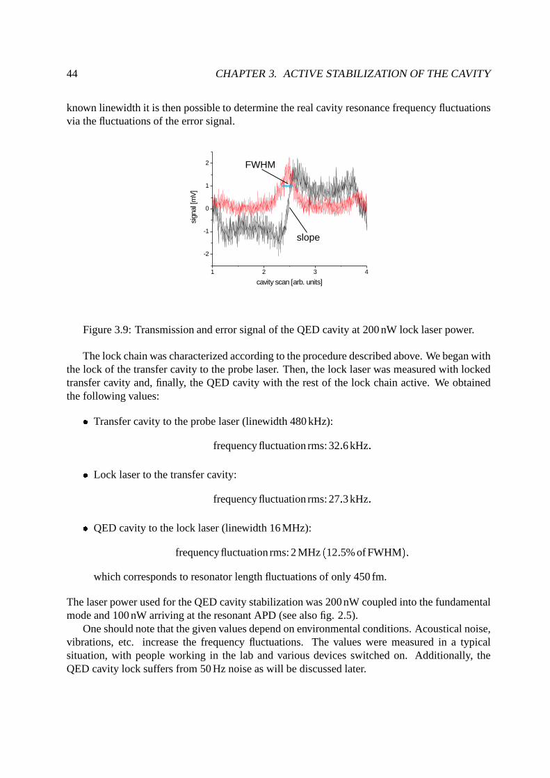
Our method to measure the frequency stability is to observe the fluctuations of the error signalwhile the feedback loop is active. They are directly related to the resonance frequency fluctu-ations. For this measurement one scans the cavity and displays simultaneously the error signaland the transmission of the corresponding laser on an oscilloscope. One measures the width ofthe transmission line together with the slope of the error signal, see fig. 3.9. These two valuesallow us to relate the error signal to the frequency deviation. Finally the stabilization is activatedand the residual root-mean-square (rms) fluctuations of the error signal are measured. With the


known linewidth it is then possible to determine the real cavity resonance frequency fluctuationsvia the fluctuations of the error signal.

1 2 3 4

-2

-1

0

1

2

sign

al[m

V]

cavity scan [arb. units]

FWHM

slope

Figure 3.9: Transmission and error signal of the QED cavity at 200 nW lock laser power.

The lock chain was characterized according to the procedure described above. We began withthe lock of the transfer cavity to the probe laser. Then, the lock laser was measured with lockedtransfer cavity and, finally, the QED cavity with the rest of the lock chain active. We obtainedthe following values:? Transfer cavity to the probe laser (linewidth 480 kHz):

frequency fluctuation rms: 32 6 kHz ? Lock laser to the transfer cavity:

frequency fluctuation rms: 27 3 kHz ? QED cavity to the lock laser (linewidth 16 MHz):

frequency fluctuation rms: 2 MHz 12 5% of FWHM which corresponds to resonator length fluctuations of only 450 fm.

The laser power used for the QED cavity stabilization was 200 nW coupled into the fundamentalmode and 100 nW arriving at the resonant APD (see also fig. 2.5).

One should note that the given values depend on environmental conditions. Acoustical noise,vibrations, etc. increase the frequency fluctuations. The values were measured in a typicalsituation, with people working in the lab and various devices switched on. Additionally, theQED cavity lock suffers from 50 Hz noise as will be discussed later.

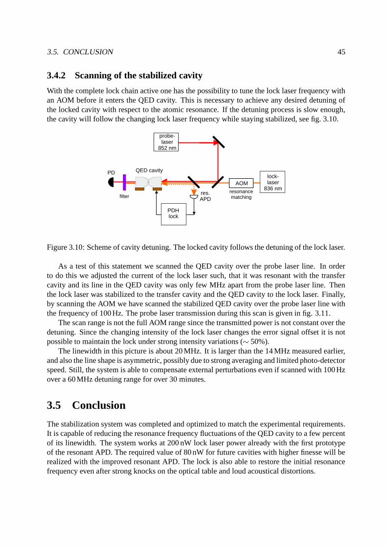
3.5. CONCLUSION 45

3.4.2 Scanning of the stabilized cavity

With the complete lock chain active one has the possibility to tune the lock laser frequency withan AOM before it enters the QED cavity. This is necessary to achieve any desired detuning ofthe locked cavity with respect to the atomic resonance. If the detuning process is slow enough,the cavity will follow the changing lock laser frequency while staying stabilized, see fig. 3.10.

lock-laser

836 nmres.APD

AOM

QED cavity

probe-laser

852 nm

resonancematching

lockPDH

PD

filter

Figure 3.10: Scheme of cavity detuning. The locked cavity follows the detuning of the lock laser.

As a test of this statement we scanned the QED cavity over the probe laser line. In orderto do this we adjusted the current of the lock laser such, that it was resonant with the transfercavity and its line in the QED cavity was only few MHz apart from the probe laser line. Thenthe lock laser was stabilized to the transfer cavity and the QED cavity to the lock laser. Finally,by scanning the AOM we have scanned the stabilized QED cavity over the probe laser line withthe frequency of 100 Hz. The probe laser transmission during this scan is given in fig. 3.11.

The scan range is not the full AOM range since the transmitted power is not constant over thedetuning. Since the changing intensity of the lock laser changes the error signal offset it is notpossible to maintain the lock under strong intensity variations ( 50%).

The linewidth in this picture is about 20 MHz. It is larger than the 14 MHz measured earlier,and also the line shape is asymmetric, possibly due to strong averaging and limited photo-detectorspeed. Still, the system is able to compensate external perturbations even if scanned with 100 Hzover a 60 MHz detuning range for over 30 minutes.

3.5 Conclusion

The stabilization system was completed and optimized to match the experimental requirements.It is capable of reducing the resonance frequency fluctuations of the QED cavity to a few percentof its linewidth. The system works at 200 nW lock laser power already with the first prototypeof the resonant APD. The required value of 80 nW for future cavities with higher finesse will berealized with the improved resonant APD. The lock is also able to restore the initial resonancefrequency even after strong knocks on the optical table and loud acoustical distortions.


Figure 3.11: Scan of the locked cavity over the probe laser resonance. The scan rate is 100 Hz,the average of 64 tracks was taken.

One of the main problems is the effect of the conveyor belt laser. Having large power (4 W),even a small part of the beam absorbed by the mirrors disturbs the stabilization due to thermaleffects. Preliminary experiments in the test chamber showed that the lock was unable to com-pensate for the mirror expansion when the laser was switched on. It has to be further considered.

Another issue remains the 50 Hz noise. It can be produced by practically any device inthe lab and is induced electronically over ground loops. Being induced onto the error signal itcauses periodic fluctuations of the resonance frequency on the order of 10% of the linewidth. Apossible way to solve this problem is the proper grounding of all involved electronic devices. Wegrounded most of the devices in direct vicinity of the setup and switched off unnecessary ones,this reduced the noise but this issue still has to be improved.

Chapter 4

Cavity ring-down

In order to achieve the best experimental parameters for our cavity, we have to select mirrors withthe best possible reflectivity. As we have seen, the characterization of the mirrors by measuringthe linewidth requires a stable resonator and a time-consuming assembly process. In our case themirrors are glued onto piezo elements and thus can not be reused. In view of the strong variationsof the mirror quality, a quicker and simpler method for measuring the finesse would be of greatadvantage. In this chapter I present a method which enables us to quickly test the mirror finesseand sort out good mirrors before the resonator is assembled.

4.1 Basic principle

The task of measuring the finesse of a mirror pair is equivalent to measuring the photon lifetimewithin the cavity. Using an assembled resonator it was done by measuring the spectral linewidthtogether with the free spectral range, see sec. 2.2.3. However, this method requires a stableresonator, mechanical and electronic noise sources make the line move or change its shape.Another possibility to infer the finesse quickly, is to directly measure the photon lifetime byobserving the decay of cavity transmission. The cavity is filled with photons by tuning it intoresonance with the laser before we switch the laser off. The photons start to leak out and thecavity field decays exponentially. The time evolution of the intensity leaking out of the cavity isgiven by eq. (1.9):

I t I t 0 e tτ

where τ 1κ is the (resonator length dependent) photon lifetime. As already shown in eq. (1.10),

τ is directly connected to the finesse:

F ∆ωFSRτ πcL

τ Thus, the observation of the intensity decay of the cavity transmission allows us to determine thetime constant τ and the finesse F .

47

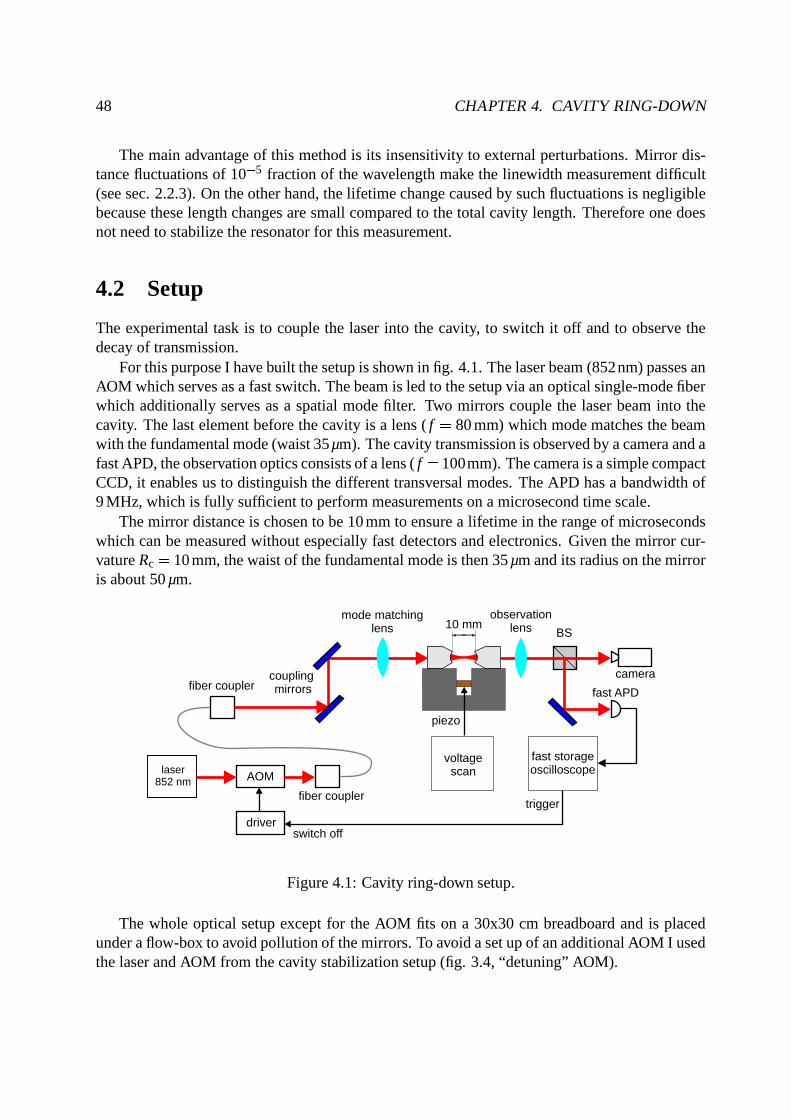
48 CHAPTER 4. CAVITY RING-DOWN

The main advantage of this method is its insensitivity to external perturbations. Mirror dis-tance fluctuations of 10 5 fraction of the wavelength make the linewidth measurement difficult(see sec. 2.2.3). On the other hand, the lifetime change caused by such fluctuations is negligiblebecause these length changes are small compared to the total cavity length. Therefore one doesnot need to stabilize the resonator for this measurement.

4.2 Setup

The experimental task is to couple the laser into the cavity, to switch it off and to observe thedecay of transmission.

For this purpose I have built the setup is shown in fig. 4.1. The laser beam (852nm) passes anAOM which serves as a fast switch. The beam is led to the setup via an optical single-mode fiberwhich additionally serves as a spatial mode filter. Two mirrors couple the laser beam into thecavity. The last element before the cavity is a lens ( f 80 mm) which mode matches the beamwith the fundamental mode (waist 35µm). The cavity transmission is observed by a camera and afast APD, the observation optics consists of a lens ( f 100mm). The camera is a simple compactCCD, it enables us to distinguish the different transversal modes. The APD has a bandwidth of9 MHz, which is fully sufficient to perform measurements on a microsecond time scale.

The mirror distance is chosen to be 10 mm to ensure a lifetime in the range of microsecondswhich can be measured without especially fast detectors and electronics. Given the mirror cur-vature Rc 10 mm, the waist of the fundamental mode is then 35 µm and its radius on the mirroris about 50 µm.

laser852 nm

fast storageoscilloscopeAOM

camera

voltagescan

fast APD

10 mm

trigger

switch off

piezo

mode matchinglens

couplingmirrors

driver

observationlens BS

fiber coupler

fiber coupler

Figure 4.1: Cavity ring-down setup.

The whole optical setup except for the AOM fits on a 30x30 cm breadboard and is placedunder a flow-box to avoid pollution of the mirrors. To avoid a set up of an additional AOM I usedthe laser and AOM from the cavity stabilization setup (fig. 3.4, “detuning” AOM).

4.2. SETUP 49

4.2.1 Mirror holder

Special care was taken to design the mirror holder. In order to simplify the coupling into the modeit should be possible to place the mirrors coaxially without much effort. This can be achieved byputting them into a V-groove. Additionally, one must also be able to scan the mirror distance totune the cavity in resonance with the laser.

The design and view of the holder are shown in fig 4.2. It is an aluminum block in whicha slit of 5 mm is cut. The slit almost cuts the whole block, only a small rest of metal holds thetwo halves together. On one side a small layer of the lower part is removed, such that this partcan be tilted. In order to scan the mirror distance, a piezo element is fixed in the slit, which isable to push the two halves apart. This piezo element (Piezomechanik PSt 150/2x3/5) is pressedwith a screw against one wall of the slit such that if the piezo contracts, the two halves approach.For better force transmission to the screw it has a spherical corundum end piece. The maximalstroke is 7µm for 150 V and with 5 10V one can scan about 1µm which covers two free spectralranges.

The main part of the holder, the V-groove, is cut in the last fabrication step to go straightthrough both halves. Now the mirrors can be simply put into the groove and are lying coaxially,assuming their shape is well cylindrical. If the mirrors had to be placed on separate holders itwould increase the degrees of freedom by 2x2, making mode matching nearly a hopeless task.With our coaxially positioned cavity mirrors the mode matching is done using two mirrors whilescanning the piezo voltage, which constitute 5 degrees of freedom in total.

mirrorspiezo

V - groove

50 mm

5 mm

slit

15 mm

38 m

m

Figure 4.2: Holder for mirrors.

In order to scan the cavity we apply to the piezo a triangle signal with variable amplitude andoffset (max. 5 10V). By these means we can tune the cavity in resonance with the laser.

When putting mirrors into the holder their distance is set manually to 10 mm with the help oftwo reference marks on the side of the holder. This distance of 10mm is also convenient, because1µs decay time corresponds approximately to a finesse of 100000. The manual adjustment of thedistance limits the precision of the finesse measurement to 5 5%, this will be discussed later.


4.2.2 Laser switching

In order to observe photon decay one has to bring the cavity in resonance with the laser and switchit off much faster than the photon lifetime. This is accomplished by scanning the cavity distanceslowly (10 100 Hz) over the laser resonance, resulting in an increase of the transmission. Thetransmission signal of the APD is sent to a storage oscilloscope. When its level reaches somedefined threshold, the oscilloscope generates a trigger signal. This signal is a standard TTLvoltage step from 0 V to +5 V. It is sent to an inverting unit (DM74LS00 logical NAND) andbecomes a step from +4 V to 0 V. This voltage is fed through an buffer amplifier (Buf634),which is a gain 1 amplifier for high power. Its output signal controls the driver (Neos N21125-1AMVCO) of the AOM (Neos 23125) which serves as a fast switch.

in outNOT BUFlogical inverter buffer amplifier

t

V

0

+5TTL trigger pulse

t

V

0

+4

to AOM driver

Figure 4.3: Inverter for laser switching.

0,0 0,5 1,0 1,5 2,0-20

0

20

40

60

80

100

120

140

160

180

AP

Dsi

gnal

,trig

gers

igna

l[m

V]

time [µs]0 50 100 150 200

-20

0

20

40

60

80

time [ns]

AP

Dsi

gnal

[mV

]

laser off

laser on

delay

trigger signal/10switching time

Figure 4.4: Laser switch-off behavior. Overview of the process on the left, zoom in on the right.

Figure 4.4 shows the switching process, taken without cavity. It shows the transmission signalof the APD and the signal one obtains without laser (zero level). Switching time below 100 nsis achieved, which is fully sufficient for our purpose. Two parameters influence the switching

4.3. MEASUREMENTS 51

time. First is the speed of electronics (inverter unit). The inverting unit was measured to giveswitching time below 25 ns. The second is the speed of the AOM driver and the relaxation in theAOM crystal itself. There a sonic wave creates a refraction index Bragg grating. This movingpattern diffracts the laser beam, the first order diffraction can be controlled by the power of thesonic wave. After the power is switched off, the grating starts to fade. The fading crosses thesite of the beam focus at the sonic velocity. For typical parameters of 30 µm waist and 3 km

s sonicvelocity it takes about 20 ns for the wave to traverse the focus.

One can see the delay of about 1 µs between the trigger signal and the beginning of theswitching process. It results from the fact that the fading has to traverse a part of the crystal (fewmm) to reach the beam focus site. Additionally there is a small run time in the cables.The laser is not completely extinguished, there is a residual intensity of less than 3%. This is dueto voltage offset produced by the inverting unit, such that the AOM control voltage does not goto zero.Additionally the APD produces a negative offset of 7mV. Another feature is that the transmissionsignal at some point falls below the the zero level. This is due to the APD which has a bandwidthof 9MHz and is working at its speed limit in this case. During the actual experiment with fall offtimes in a microsecond range this effect does not occur.

4.3 Measurements

4.3.1 Procedure

After the mirrors are put into the holder, there are two tasks to accomplish: mode matching andthe observation of decay.

Mode matching: We work with the fundamental mode of the cavity, which illuminates a welldefined spot on the mirror surface in a homogeneous way. In order to do this we need to couplemost of the intensity into this mode to ensure high transmission. It is achieved by means of twomirrors placed before the resonator and controlling beam position and angle. The transmission isobserved with a camera making possible to distinguish between the different transversal modes.

Practically, we switch to a small scan range and slow scan rate (at 10 Hz the eye can see evenweak mode transmission blinks). We change the offset slowly, moving through the free spectralrange and observing the transmission with the camera. Usually at least one higher transversemode should be visible without adjustments. Then we can optimize this mode using one mirrorand look in its vicinity for the neighboring lower transversal mode. We optimize this mode andmoves on. By these means one can proceed to the fundamental mode. The scan is switched to100 Hz and the fundamental mode coupling is then optimized with both mirrors.

This procedure requires some experience, the time needed for one measurement stronglydepends on how easy one can find and optimize the fundamental mode. Typical times rangebetween 5 and 20 minutes.

Observation of ring-down: After optimizing the coupling, the trigger of the storage oscillo-scope is set to a possibly high value. This means that the transmission of the fundamental modewhen scanning over the resonance should hardly reach this level. This provides a high signal


level and also the other modes do not trigger the measurement. Each time the transmission goesbeyond trigger level the laser is switched off. The decay of the transmission is recorded withthe storage oscilloscope and averaged over 64 measurements to increase the signal to noise ratio.Recording 64 decay curves takes less than one minute.

Accumulating and taking the mean value over several measurements with (in principle) vary-ing intensity and trigger time is possible because of the properties of the exponential:

I1e tτ I2e t

τ I1 I2 e tτ

and

Ie t H t0τ Ie t1 H t0

τ e t H t1τ I I e t H t1

τ Therefore the measurement of the time constant is not influenced by the absolute intensity andthe time of the trigger. The residual intensity of the laser produces a (constant) offset which isagain of no importance for the measurement.

4.3.2 Analysis

Figure 4.5 shows a typical measured decay curve, averaged over 64 measurements. The triggersignal is sent at t 0 and after about 1 µs the transmission begins to decay. As expected, thedecaying part of the curve has an exponential shape.

Figure 4.5: Decay of the transmission. The big points show the exponential fit.

We fit a function of the form f t A e tτ y0 to the decay, where y0 counts for the APD

offset and residual laser intensity. The range of the fit begins about 500 ns after the switch-off


to exclude the switching process and to observe pure decay. The resulting quality of the fit isextremely high and does not limit the precision as we will see later.

4.3.3 Precision limits and reproducibility

In the following we will consider the factors which influence the measurement the lifetime.? Mirror distance: Since the distance of 10 mm between the mirrors is adjusted manuallywith the help of reference marks on the holder, variations on the distance will occur. Toestimate this error, the decay time τ was measured several times, one mirror being moveda bit and then readjusted again to the 10 mm distance.

# 1 2 3 4 5 τ στ : ns < 855 833 833 883 942 869.2 40.7

Table 4.1: Distance reproducibility measurement (βB3 vs βA3).

One can see that the reproducibility in this case is pretty high. The standard deviation of thisset is σ 40 7 ns which is about 5% of the mean value. This corresponds to length deviation of0 5mm. Still, this is the main limit of the precision of the finesse measurement, since the fit erroris order of a magnitude smaller.? Mirror rotation: If the mirrors are not perfectly coaxial within the groove, the mode is

not exactly centered. Thus the mirror rotation exposes a different spot on the surface. Ourexperience with these mirrors shows, that the surface quality is extremely inhomogeneous(scratches, dust particles, etc.). The measurement below shows an example of repeatedmeasurements after rotations of one of the mirrors (about 30 J ).

# 1 2 3 4 5 τ στ : ns < 925 886 913 354 806 776.8 215.4

Table 4.2: Measurement with rotation of one mirror, mirror pair βB3 vs βA3.

The large spread in the values shows that different spots of the mirror surface have differentquality. Since the mirrors are not exactly coaxial, the rotation of one mirror moves the position ofthe surface a bit, which can also be seen with the camera. The resulting difference in finesse canbe larger than 50% for a mirror pair. It can be due to the presence of single larger dust particleson the surface within the mode, but also a larger number of small spots may have the same effect.

We repeated the measurement with another mirror pair. Here the spread is very small and lieswithin the length precision. These mirrors have better finesse together a better homogeneity.


# 1 2 3 4 5 τ στ : ns < 1020 1019 1050 1064 1119 1054.4 36.6

Table 4.3: Measurement with rotation for the mirror pair βD3 vs βB3.

One important observation is the correlation of transmission and finesse: in most cases hightransmission was accompanied by better finesse. The absolute transmission depends on the de-gree of mode matching, so this effect was not observed systematically. On the other hand mirrorpairs with low transmission usually show relatively low finesse. This indicates that the dominat-ing factor for the finesse are the losses. These could be either inherent (within the coating) ordue to surface damage or pollution.

4.3.4 Characterization of a mirror set

Now we apply the method to our set of mirrors. We possess 18 mirrors which were cleaned bythe manufacturer. We divided them into 3 sets of 6 mirrors, each set in a separate box. The boxescontain 5x5 grid of holes where mirrors can be placed. The boxes are signed α β γ and the gridchess-board-like A-E, 1-5.

The first step is to inspect the mirror surface with the help of a microscope (500x, dark-field). This is necessary to find a mirror with as homogeneous surface as possible. This mirrorcan then be used as a reference, i.e. we can measure all the other mirrors with this one. Finessevariations due to different mode spot positions will then mostly depend on the other tested mirror.Another reason for visual inspection is to try finding the dependence of measured finesse onvisible surface condition. The inspection showed that most of the mirrors have many small spotsand/or scratches in the center region (radius 0 25 mm). Many of them had even macroscopicparticles. All mirrors had at least a few spots in the center. According to our previous criteria ofthe old visual method even the best mirrors are imperfect. Still we found a mirror with only fewspots in the center region which also were more or less equally distributed. We took this mirror βE3 as a reference.

In the box β each of the five remaining mirrors was tested with the reference mirror 4 times,rotating the mirror after each measurement. The mirrors with the best performance in this testwere then measured together. The results are shown in tab. 4.4.

As discussed above, the error of this measurement is about 5%. We see, that the mirror βE3showing good surface quality which was chosen as the reference does not have the best finesse inthis case. This shows that the visual inspection of the mirror surface gives only a coarse measurefor the finesse.

Then we tested the boxes α and γ versus the reference mirror. The results are given in thetables. As one can see, 10 out 18 mirrors are far below the specification of 100000. If it is due tobigger dust particles on the surface which were visible under the microscope, the situation maybe improved by cleaning.

The pair αE1 αD2 yields a finesse of 180000. This is 50% better than the mirrors whichare currently assembled in our test vacuum setup.


βA3 βB3 βC3 βD3 βE3 βA4βA3 83500βB3 94100βC3 98500βD3 111900 108500 117000βE3 -βA4 89200

Table 4.4: Best finesse for mirror set ß

αA1 αC1 αE1 αB2 αD2 αA3 βE3αA1 106400αC1 44600αE1 182900 111000αB2 46900αD2 131800αA3 51500

Table 4.5: Best finesse for mirror set α

γA1 γC1 γE1 γB2 γD2 γA3 βE3γA1 82400γC1 111200γE1 81200γB2 63200γD2 51500γA3 118900 103900

Table 4.6: Best finesse for mirror set γ

Conclusion

I have implemented a compact and easy to use setup for fast mirror characterization. It is capableof measuring the mirror finesse quickly and with precision of about 5%. Applying it to the setof our mirrors I found a mirror pair with a considerably better finesse, than we currently have inour assembled resonator. The process of finding good mirrors for future resonators will be fastand reliable.

Summary and outlook

The goal of this work was to prepare a high finesse optical resonator for cavity QED experi-ments. The preparation includes finding mirrors of best reflectivity, building and characterizingthe resonator and achieving the necessary stability for future experimental conditions.

Considering the amount of work for visually inspecting the mirrors and assembling the res-onator we needed a method to characterize the mirrors quickly. I have implemented the setupfor cavity ring-down, which measures the lifetime of photons in the cavity. It has the advantagethat it does not require a stable assembled resonator. Instead, the mirrors are put into a speciallydesigned holder which allows to align them reducing the amount of work substantially. With thissetup we characterized our whole mirror set within a short time. It allows us to sort out mirrorswith the best reflectivity and will be of a great advantage for setting up new resonators.

We have set up and characterized a resonator with length L 92µm and finesse F 118000.The obtained parameter set is g κ Γ 2π 40 3 14 5 2 MHz, which means that we canachieve the regime of strong coupling where the coherent atom-photon interaction g is largerthan the incoherent loss processes κ Γ.

Continuing the work of Y. Miroshnychenko [Mir02], we completed, optimized and charac-terized the cavity stabilization scheme. We have solved the problem of mechanical resonancesof the piezo elements and implemented the resonantly amplified APD which is a highly sensitivedetector for stabilization purposes. Finally we have shown that the system is able to stabilize thecavity to 12% of the linewidth under conditions of low lock laser power (200 nW).

The next steps will be the placement of the cavity into the main setup and transport of an atominto the cavity. The detection of an atom in the resonator can be performed by a measurement ofthe Rabi splitting of atom and cavity resonances. A major difficulty of this experiment will bethe alignment of the conveyor belt laser which must fit through the small slit between the mirrorsand connect the MOT with the cavity mode which have both a size of only about 30 µm and are5 mm apart. Finally, after the deterministic transport of two atoms into the cavity mode, we willbe able to realize a controlled atom-atom interaction which is a step towards a quantum logicgate.

56

Appendix A

Solution of the master equation

Enter the matrix

We begin with the master equation (1.13).

ddt

&ρ 1

i ';: &H &ρ <, κ2 2aρa† a†aρ ρa†a Γ

2 2σρσ† σ†σρ ρσ†σ with &

H ' ω0 ωl σ†σ -' ωc ωl a†a =' g σ†a σa† =' ε a† a Now we use the weak field approximation. In this regime the driving field ε is so small, thatat most one excitation in the system is present. Therefore we consider only three states of thesystem: g ) 1 ) e ) 0 ) g ) 0 ) Here, g ) e ) are the atomic ground and excited state, 0 ) 1 ) are states with zero and one photonin the cavity.Calling these states 1, 2, 3 respectively, we define the 3 by 3 density matrix:/1

ρ11 ρ12 ρ13

ρ21 ρ22 ρ23

ρ31 ρ32 ρ33

24 This matrix is Hermitian, i.e. ρmn ρ Cnm.The corresponding creation and annihilation operators are:

a† g ) 1 )K+ g + 0 /10 0 10 0 00 0 0

24 a g ) 0 )L+ g + 1 /10 0 00 0 01 0 0

24 σ† e ) 0 )K+ g + 0 /1

0 0 00 0 10 0 0

24 σ g ) 0 )K+ e + 0 /10 0 00 0 00 1 0

24 57

58 APPENDIX A. SOLUTION OF THE MASTER EQUATION

The dissipation in the system leads to a stationary state with

ddt

&ρ 0

This leads to a system of 9 homogeneous complex equations from which 6 are independent: κρ11 i g ρ12 ρ C12 ε ρ13 ρ C13 0 ig ρ12 ρ C12 Γρ22 0

κρ11 Γρ22 iε ρ13 ρ C13 0 12 Γ κ ρ12 i g ρ11 ρ22 ερ C23 ω0 ωc ρ12 0 κ

2ρ13 i ε ρ11 ρ33 gρ23 ωc ωl ρ13 0 Γ2

ρ23 i gρ13 ερ C12 ω0 ωl ρ23 0 Now we separate the real and imaginary parts, ρmn Rmn iImn, getting 9 real equations,

which can be written as a matrix:MNNNNNNNNNNNNNNNNOκ2 0 0 0 g 0 ε 0 0

0 Γ2 0 0 P g 0 0 0 0

κ2

Γ2 0 0 0 0 ε 0 0

0 0 0 PRQ Γ2 S κ

2 T PRQ ω0 P ωc T 0 0 0 P εg P g 0 Q ω0 P ωc T PRQ Γ

2 S κ2 T 0 0 P ε 0

0 0 0 0 0 P κ2 Q ωc P ωl T 0 g

ε 0 P ε 0 0 PRQ ωc P ωl T P κ2 P g 0

0 0 0 0 ε 0 g P Γ2 Q ω0 P ωl T

0 0 0 ε 0 P g 0 PRQ ω0 P ωl T P Γ2

UWVVVVVVVVVVVVVVVVXYMNNNNNNNNNNNNNNNNO

R11

R22

R33

R12

I!2

R13

I13

R23

I23

UWVVVVVVVVVVVVVVVVXZMNNNNNNNNNNNNNNNNO

0

0

0

0

0

0

0

0

0

UWVVVVVVVVVVVVVVVVXThis system was solved with the help of a mathematics program. The resulting expressions

are long and contain different combinations of the matrix coefficients. We do not write themdown here. In the next step all terms which contain ε in a higher than first order are consequentlyneglected .

To obtain the populations of atom and cavity we need only R11 R22 and R33. We see that inour approximation R11 R22 % R33, thus we can norm the density matrix by setting ρ11 R11

R33and

ρ22 R22R33

.

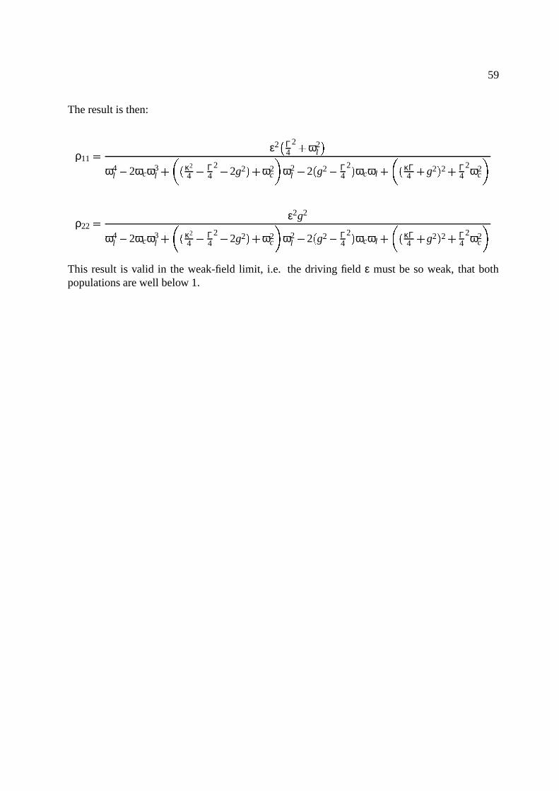
59

The result is then:

ρ11 ε2 Γ4

2 ω2l

ω4l 2ωcω3

l κ2

4 Γ4

2 2g2 ω2c ω2

l 2 g2 Γ4

2 ωcωl κΓ4 g2 2 Γ

42ω2

c ρ22 ε2g2

ω4l 2ωcω3

l κ2

4 Γ4

2 2g2 ω2c ω2

l 2 g2 Γ4

2 ωcωl κΓ4 g2 2 Γ

42ω2

c This result is valid in the weak-field limit, i.e. the driving field ε must be so weak, that bothpopulations are well below 1.

Bibliography

[Mir02] Y. Miroshnychenko: “Design and test of an optical high finesse resonator for singleatom experiments”, diploma thesis at University of Bonn, 2002

[Car93] H. Carmichael, “An open systems approach to quantum optics”, Springer 1993

[Sch01] D. Schrader, S. Kuhr, W. Alt, M. Mueller, V. Gomer and D. Meschede, “An opticalconveyor belt for single neutral atoms”, Appl. Phys. B 73(8), p. 819 (2001)

[Kuhr01] S. Kuhr, W. Alt, D. Schrader, M. Muller, V. Gomer and D. Meschede, “Deterministicdelivery of a single atom”, Science 293, 278

[Kuhr03] S. Kuhr, “A controlled quantum system of individual neutral atoms”, dissertation atUniversity of Bonn, 2003

[Dot02] I. Dotsenko: “Raman spectroscopy of single atoms”, diploma thesis at University ofBonn, 2002

[Jay63] E. Jaynes and F. Cummings, Proc. IEEE 51. p. 89 (1963)

[Sie86] A. Siegman, “Lasers”, University Science Books, California (1986)

[Shor94] P.W. Shor, “Discrete logarithms and factoring”, Proc. 35th Annual Symp. on Founda-tions of Computer Science, Nov. 1994, pp. 124-134

[Dre83] R. Drever and J. Hall, “Laser phase and frequency stabilization using an optical res-onator”, Appl. Phys. B 31, p. 97 (1983)

[Tan02] Sze M. Tan: “Quantum optics and computation toolbox for Matlab”

[Ste98] D. A. Steck: “Cesium D Line Data”

[Sho90] B. W. Shore: “The theory of coherent atomic excitation”, vol. 1, Wiley 1990

[Scu97] M. O. Scully, M. S. Zubairy: “Quantum optics”, Cambridge university press, 1997

[Osn01] S. Osnagi, P. Bertet, A. Auffeves, P. Maioli, J.M. Raimond and S. Haroche: “Coherentcontrol of an atomic collision in a cavity”

60

BIBLIOGRAPHY 61

[Lieb03] D. Liebfried, R. Blatt, C. Monroe, D. Wineland, “Quantum dynamics of single trappedions”, Reviews of Modern Physics, V. 75, Jan. 2003

[Yi02] X. X. Yi, X. H. Su and L. You: “A conditional quantum phase gate between two 3-stateatoms”, quant/ph 0210160

Acknowledgements

The year of my diploma work is now over and I want to thank all the people who helped andsupported me during this time. I want to thank

the “single-atoms” team, in particular:Dominik Schrader for teaching me all things I needed in the lab and forgiving even my most

stupid mistakes,Wolfgang Alt for being able to answer all my questions, showing new ways when I was stuck,

and his endless patience with me,Dr. Stefan Kuhr for his endless energy and optimism, even during night measurements,Yevhen Miroshnychenko and Igor Dotsenko for their help in my work and nice time spent

together,Mika Khudaverdyan for punching me every time I was about to lose my sense of humor,

these people work hard and enthusiastic on this complex and fascinating experiment;

all other members of the group for the friendly atmosphere,Prof. Dr. D. Meschede for providing me access to all this,Prof. Dr. K. Buse for being my coreferent,

my parents for their endless love and support,my sensei Jury Jukelis for sharing his strength with me,and Julia Mark for dreaming the Venice dream with me.

Thank you!Wenjamin Rosenfeld, August 2003

A high finesse optical resonator for cavity QED experiments

Documents