A Hierarchy of Approximations of the Master Equation Scaled by a Size Parameter

A HIERARCHY OF APPROXIMATIONS OF THE

MASTER EQUATION SCALED BY A SIZE

PARAMETER

LARS FERM1, PER LOTSTEDT1, ANDREAS HELLANDER1 1Division of Scientific Computing, Department of Information Technology

Uppsala University, SE-75105 Uppsala, Sweden

emails: [email protected], [email protected], [email protected]

Abstract

Solutions of the master equation are approximated using a hierarchy ofmodels based on the solution of ordinary differential equations: the macro-scopic equations, the linear noise approximation and the moment equa-tions. The advantage with the approximations is that the computationalwork with deterministic algorithms grows as a polynomial in the numberof species instead of an exponential growth with conventional methods forthe master equation. The relation between the approximations is inves-tigated theoretically and in numerical examples. The solutions convergeto the macroscopic equations when a parameter measuring the size of thesystem grows. A computational criterion is suggested for estimating theaccuracy of the approximations. The numerical examples are models forthe migration of people, in population dynamics and in molecular biology.

Keywords: master equation, reaction rate equations, linear noise approx-imation, moment equations

AMS subject classification: 37M05, 34E10, 65C50

1 Introduction

The master equation (ME) is an equation for the time evolution of the probabilitydensity function (PDF) for the copy numbers of different species in systems withan intrinsic noise [18, 25]. The systems are modeled as Markov processes withFinancial support has been obtained from the Swedish Foundation for Strategic Researchand the Swedish Graduate School in Mathematics and Computing.

1

discrete states in continuous time. Analytical solutions of the ME are known onlyunder simplifying assumptions. Most systems call for a numerical solution of thegoverning equation. Examples where the ME is used as a model are in stochasticprocesses in physics and chemistry [17, 20, 25], population dynamics in ecology[5, 11, 31], the spread of infectuous disease in epidemiology [4, 37], molecularbiology [9, 10, 29, 30], and the social sciences [41, 42]. Modeling on a mesoscalelevel with the ME is necessary in these applications if the copy number of eachspecies is low and stochastic fluctuations are important. If this number is largethen a macroscopic equation for the mean values is often satisfactory.

A computational difficulty with the ME is that the dimension of the prob-lem is the same as the number of participating species. The number of differentstates that the system can reach grows exponentially with increasing number ofspecies making direct numerical solution of the ME impossible for more than afew species. The most popular method for computing the solution is due to Gille-spie [20]. His Stochastic Simulation Algorithm (SSA) is a Monte Carlo methodfor simulation of a time dependent trajectory of a system. From a collection oftrajectories, statistical properties can be determined such as mean values, vari-ances, and PDFs. Since SSA is a Monte Carlo method, the convergence is slowin particular if we are interested in the PDF. The progress in time is also slow ifthe problem has at least two different time scales and the slow scale models thelong term dynamics but the fast scale restricts the time steps. Modifications ofSSA suitable for stiff problems have been developed [3, 7].

Deterministic algorithms have the advantage of fast convergence and for low-dimensional problems they are superior to SSA [36]. For systems with manyspecies, approximations are necessary for solution of the ME using the moments[12] or the related Fokker-Planck equation [18, 25, 35] to avoid the exponentialgrowth [28]. Usually, there is a size parameter associated with the ME model.It is a measure of the copy numbers of the species or a volume or an area in themodel. If the system size is large, the model behaves like a macroscopic systemgoverned by a system of nonlinear ordinary differential equations (ODEs) for theconcentrations of the species [18, 25]. The number of equations is then equal tothe number of species and numerical solution is possible for systems with manyspecies. If the copy numbers are small, then only a mesoscopic model given bythe ME is sufficiently accurate. In the intermediate range between large andsmall, there are other equations approximating the ME without suffering fromthe exponential increase in the computational work. Three of these equationsare investigated in this paper and their suitability for numerical approximationof the ME is evaluated.

It is difficult to know a priori if an approximation is accurate or not. Theerror in the approximation is here quantified by inserting the approximationsinto the ME. The norm of the residual is a measure of the quality of the solution.Such a posteriori error estimation is found in other applications, see e.g. [33].The sum in the norm of the residual for high-dimensional problems is computed

2

by a Quasi Monte Carlo method [2].Similar techniques with expansions in a small parameter and moment equa-

tions are utilized in high frequency electromagnetics [13]. The moment equationsobtained after expansion of the Boltzmann equation in the small Knudsen numberare the Euler and Navier-Stokes equations of fluid flow [39]. In turbulence modelsin computational fluid dynamics [43], higher moments of the fluctuating flow areapproximated for closure of the equations. A review article where macroscopicproperties are derived from microscopic and stochastic descriptions is found in[21].

In the next section, the ME and the approximating equations and the relationbetween them are discussed. The convergence of the solution of the equationsfor the expected values and the covariances to the solution of the macroscopicequations is proved in Section 3. A method to compute the errors in the MEcaused by the approximations is suggested in Section 4. The numerical resultsare reported in Section 5. The methods are applied to one problem from the socialsciences [41], a well known model in population dynamics with foxes and rabbits[32], a system of two metabolites interacting with two enzymes in biochemistry,and a molecular clock in biology [1, 40]. Conclusions are drawn in the finalsection.

The notation in the paper is as follows. The i:th element of a vector v isdenoted by vi. If vi 0 for all i, then we write v 0. The Einstein summationconvention is adopted so that summation is implied over an index appearing twicein a term. The space derivative of vi(x) with respect to xj is denoted by vi;j. Thetime derivative p=t of p(x; t) is written pt and q is a shorter notation for dq=dt.The `-norm of v of length N is kvk = (

PNi=1 jvij)1=. The Euclidean vectornorm, = 2, is denoted by kvk =

pvivi. The corresponding Euclidean normsfor multi-index tensors are e.g. kAk2 = AijAij = trATA and kBk2 = BijkBijk.The set of integer numbers is written Z and Z+ denotes the non-negative integernumbers. In the same manner, R denotes the real numbers and R+ is the non-negative real numbers.

2 The approximating equations

The system we are considering has N interacting species Xi; i = 1; : : : ; N , andthe copy number of species Xi is denoted by xi. The state vector x is time-dependent and a transition r from one state xr to x occurs with the probabilitywr(xr; t) per time unit. The change in the state vector by a transition is written

xr wr(xr;t)! x; nr = xr x: (1)

The difference nr between the states before and after the transition has only a fewnon-zero components and nr 2 ZN. In chemistry, xi is the number of molecules of

3

species i and wr(xr; t) is the propensity for reaction r to take place. In populationdynamics, xi is the number of individuals of species i. As an example, a new copyof a species may appear or disappear in a transition from one state to another.

The systems are assumed to have a scaling with a size parameter Ω as in[25, 26] which is large compared to 1 and " = Ω1 1. In chemical applications,Ω can denote a volume and in population dynamics an area. Then yi = xi=Ω isinterpreted as the concentration or population density of species i. The propen-sities for r = 1; : : : ; R; fulfill the following assumption.

Assumption 1. The propensities have continuous third derivatives in space andtime, wr 2 C3[x 0; t 0], and can be writtenwr(x; t) = Ωvr(Ω1x; t) = Ωvr(y; t);where vr and its derivatives in yi are of O(1).

Equations for simulation of the dynamics of a system with transitions betweenstates (1) occurring with probabilities wr satisfying Assumption 1 are given below.

2.1 The master equation

At a mesoscopic level with intrinsic noise in the system, the probability densityfunction (PDF) p(x; t) for the system to be in the state x at time t satisfiesthe ME [18, 25] and xi is a non-negative integer number, x 2 ZN

+ . Introduce asplitting of nr into two parts so that

nr = n+r + nr ; n+ri = max(nri; 0); nri = min(nri; 0):Then the ME for R different transitions ispt(x; t) =

RXr = 1

x + nr 0

wr(x + nr; t)p(x + nr; t) RXr = 1

x n+r 0

wr(x; t)p(x; t) (Mp)(x; t); (2)

defining the master operatorM. The total probabilityP

x2ZN+p(x; t) is preserved

in time with these boundary conditions at xi = 0 [16].Direct numerical solution of the ME after approximation of the time derivative

is prohibitive if N is greater than four or five. Suppose that the maximum copynumber for all species is xmax. Then the size of the state space is (xmax +1)N andit grows exponentially with N . Already with xmax = 100 and N = 5 the statespace is quite large.

2.2 The macroscopic equation

The equations for the expected values mi of xi with the PDF satisfying (2) are asystem of nonlinear ODEs. They are the governing equations of the dynamics ofthe system at a macroscopic level.

4

By multiplying (2) by xi and summing over ZN+ , the equation for mi = E[Xi] 2R is [12, 25]mi = nriE[wr(X; t)]: (3)

If every wr is linear in X thenE[wr(X; t)] = wr(E[X]; t) = wr(m; t);and the system (3) is closed. If this is not the case, then the macroscopic approx-imation isE[wr(X; t)] wr(m; t)and we arrive atmi = nriwr(m; t) !i(m; t): (4)

These are the reaction rate equations in chemical kinetics.The corresponding equations for the mean values i = mi=Ω of the concen-

trations yi follow from Assumption 1i = nrivr(; t) i(; t): (5)

The number of equations is N and the computational work to solve (4) or (5)grows as a polynomial in N of low degree depending on ! or and the numericalmethod.

2.3 The linear noise approximation

van Kampen simplified the ME by a Taylor expansion of the state variables xiaround the mean values i of the concentrations and i modeling the stochasticvariation about i as in [9, 24, 25]. The fluctuations in x are of O(Ω1=2) and therelation between x;, and is

x = Ωy = Ω(+ Ω1=2) (6)

with y;; 2 RN . Replace x in the ME and use Assumption 1 to obtainpt(Ωy; t) =Pr Ω(vr(y + Ω1nr; t)p(Ω(y + Ω1nr); t) vr(y; t)p(Ωy; t)):

(7)

Introduce

Π(; t) = p(Ω+ Ω1=2; t) = p(x; t)5

into (7) and expand the right hand side into a Taylor series around . Let thesum of terms proportional to Ω1=2 be zero. Then we arrive at the macroscopicequation (5) for .

The terms of O(1) in (7), ignoring terms of order Ω1=2 and smaller, are

Πt =Xr Πvr;inri + Π;inrivr;jj + 0:5vrnrinrjΠ;ij;

where vr and vr;i are evaluated at (t) from (5). WithVij(; t) =Xr nrinrjvr(; t); (8)

the PDE for Π(; t) is simplified to

Πt = i;j(jΠ);i + 0:5VijΠ;ij: (9)

It is shown in [24], [35, p. 156] that the solution Π of (9) is the PDF of anormal distribution

Π(; t) =1

(2)N=2p

det Σexp(0:5i(Σ1)ijj)

=1

(2)N=2p

det Σexp(0:5(xi Ωi)((ΩΣ)1)ij(xj Ωj)); (10)

where the covariance matrix is the solution of

Σij = i;kΣkj + j;kΣki + Vij: (11)

The definitions of i;j((t); t) and Vij((t); t) are found in (5) and (8). The linearnoise approximation (LNA) consists of a normal distribution with variance Σ in(11) following the track of the expected value Ω satisfying the macroscopicequation (5). The dynamics of LNA in (5) and (11) is insensitive to Ω.

There are N non-linear ODEs to solve in (5) for . The covariance matrix Σ issymmetric and we have to solve (N+1)N=2 linear ODEs in (11). The alternativeto solve the PDE in (9) with a standard deterministic algorithm suffers from theexponential growth in N in work and storage.

2.4 The two-moment equations

Let us return to (3) for a more accurate approximation of the right hand sidethan in (4) and let wr satisfy Assumption 1. Then !i(x; t) in (4) shares thisproperty and expand this function about the mean value m as in [12]!i(x; t) = !i(m; t) + !i;j(xj mj) + 0:5!i;jk(xj mj)(xk mk)

+ijkl(xj mj)(xk mk)(xl ml);ijkl = 0:5 Z 1

0

(1 )2!i;jkl(m + (xm); t) d: (12)

6

This form of the remainder term is found in [6, p. 190]. Then the expected valueof !i(X; t) isE[!i(X; t)] = !i(m; t) + 0:5!i;jkPx

(xj mj)(xk mk)p(x; t) + i;i =P

xijkl(xj mj)(xk mk)(xl ml)p(x; t):

The covariance matrix C is symmetric and defined byCij = E[(Xi mi)(Xj mj)] =X

x

(xi mi)(xj mj)p(x; t):Thus, a more accurate equation than (4) for mi is derived from (3) (cf. [12])mi = !i(m; t) + 0:5!i;jk(m; t)Cjk + i: (13)

The remainder term i vanishes if ! is at most quadratic in x.According to [12], Cij satisfiesCij = E[(Xi mi)!j(X; t)] + E[(Xj mj)!i(X; t)] + E[Wij(X; t)];Wij(x; t) =

Pr nrinrjwr(x; t):(14)

With the same expansion as in (12), we have thatE[(Xi mi)!j(X; t)] = !j;kCik + Qij;Qij =P

xRjkl(xi mi)(xk mk)(xl ml)p(x; t);Rjkl =

Z 1

0

(1 )!j;kl(m + (xm); t) d;andE[Wij] = Wij(m; t) + 0:5Wij;klCkl + Sij;Sij =

PxRijkl`(xk mk)(xl ml)(x` m`)p(x; t);Rijkl` = 0:5 Z 1

0

(1 )2Wij;kl`(m + (xm); t) d:Hence, (14) can be writtenCij = !j;kCik + !i;kCjk + Wij(m; t) + 0:5Wij;klCkl + Qij + Qji + Sij: (15)

If wr is at most quadratic in x then Sij = 0 in (15), i = 0 in (13), and Rjklin Qij depends only on time. Then Qij = RjklDikl, where Dikl is the thirdcentral moment. The ODE for Dikl has terms including the fourth moment andso on. For closure we assume that central moments of order higher than threeare negligible. Then the approximation of p is also a normal distribution as in(10)p(x; t) =

1

(2)N=2p

det Cexp(0:5(xi mi)(C1)ij(xj mj)); (16)

7

It follows from Assumption 1 that by replacing ! and W by and V andneglecting Qij and Sij in (15) we arrive atCij = j;kCik + i;kCjk + ΩVij(m=Ω; t) + 0:5Ω1Vij;klCkl: (17)

If Cij(y; 0) is of O(Ω), then from (17) we conclude that Cij(y; t) will remain ofO(Ω) in a finite time interval. With Σ = Ω1C, the ODE for Σ is

Σij = j;kΣik + i;kΣjk + Vij + 0:5"Vij;klΣkl: (18)

The difference from the equation in (11) is the last term. Introduce the samescaling of m and C in (13). Then satisfiesi = i(; t) + 0:5"i;jk(; t)Σjk; (19)

which is the reaction rate equation (5) with an additional, small term dependingon the variance. The equations (19) and (18) are the two-moment approximation(2MA) of the ME. They differ from the LNA equations in the dependence of on the variance and the dynamics depending on " and Ω.

3 Analysis of the approximating equations

The stochastic variable X with the PDF solving the master equation is firstcompared to the macroscopic solution in (5). Then the expected values and thecovariances obtained with the linear noise approximation (LNA) and the two-moment approximation (2MA) are compared to each other and to the macro-scopic solution.

3.1 The macroscale and the mesoscale models

Let Xi(t); i = 1; : : : ; n; be the stochastic variables with the PDF p(x; t) solving(2). Suppose that the propensities satisfy Assumption 1 with the size parameterΩ. If the initial conditions are such that limΩ!1Ω1X(0) = (0), then it isproved by Kurtz in [26] that

limΩ!1 P (supst kΩ1X(s) (s)k > Æ) = 0 (20)

for any Æ > 0 in a finite time interval. For large Ω, the stochastic variables arevery well approximated by the mean values from the macroscopic model. Theresult is similar to the law of large numbers.

In another theorem in [27], Kurtz derives an estimate resembling the centrallimit theorem. Let ZΩ(t) be the scaled difference between Ω1X(t) and (t)

Ω1=2ZΩ = Ω1X ; (21)

cf. (6). Suppose that the initial conditions on X and are as above. ThenZΩ converges in a finite interval when Ω !1 to a Gaussian diffusion Z(t) withmean 0 and a covariance depending on V (see Section 3.2).

8

3.2 The LNA and the 2MA

The equation for the expected values and the second moments for the 2MA arein Section 2.4i = i(; t) + 0:5"i;jk(; t)Σjk;

Σij = j;k(; t)Σik + i;k(; t)Σjk + Vij(; t) + 0:5"Vij;kl(; t)Σkl: (22)

Proposition 1. Assume that the propensities satisfy Assumption 1. Then asolution ;Σ exists to (22) for any " in an interval around t = 0.

Proof. By the assumption, i; j;k; i;jk; Vij, and Vij;kl are continuously differen-tiable and the result follows from [6, p. 283].

Let us expand the solution of (22) in the small parameter "i = 0i + "1i;Σij = Σ0ij + "Σ1ij: (23)

The terms 0i and Σ0ij in (23) satisfy the equations given by the terms of zeroorder in " in (22)0i = i(0; t); (24a)

Σ0ij = j;k(0; t)Σ0ik + i;k(0; t)Σ0jk + Vij(0; t): (24b)

These are the equations (5) and (11) for the moments in the linear noise approx-imation in Section 2.3.

Let Æij be the Kronecker tensor and let Φij(t; s); t s; satisfy

Φij(t; s) = i;kΦkj; Φij(s) = Æij;with the solution

Φij(t; s) = (exp(

Z ts 0(u) du))ij; (25)

where 0 is the gradient matrix with ( 0)ij = i;j. Using (25), the covarianceΣ0 with the initial condition Σ0(0) in (24b) with Φij = Φij(t; 0) can be writtenexplicitly [24]

Σ0ij(t) = ΦikΣ0kl(0)ΦTlj + Φik Z t0

(Φ1)klVl`(ΦT )`m ds ΦTmj= ΦikΣ0kl(0)ΦTlj +

Z t0

Φil(t; s)Vl`(s)ΦTj(t; s) ds: (26)

The mean value in (21) satisfies (24a) and the expression for the covariancesof Z is (26) [14, Ch. 11] and it satisfies (24b).

9

For the boundedness of Σ0 when t grows we need a second assumption.

Assumption 2. The propensities are such thatxii;jxj xixi; < 0;in a neighborhood of 0 for all t 0 and any x.

The stability of 0i and Σ0ij in LNA when t ! 1 is guaranteed in thefollowing proposition. A quantity is bounded if it is bounded in the k k-norm.

Proposition 2. Assume that the propensities satisfy Assumptions 1 and 2 whent 2 T = [0;1) and that 0 in (24a) is bounded in T . Then Σ0 is also boundedin T . Let 0 + Æ be the solution of a perturbed (24a)0i + ˙Æi = i(0 + Æ; t) + i; Æ(0) = Æ0:If the term on the right hand side is bounded in T and Æ0 is so small thatAssumption 2 is valid at t = 0, then Æ is also bounded in T .

Proof. Multiply (24) by Σ0ij to obtain

Σ0ijΣ0ij = kΣ0kkΣ0kt = Σ0ijj;kΣ0ki + Σ0jii;kΣ0kj + Σ0ijVij(0; t) 2kΣ0k2 + kΣ0kkVk;using the Cauchy-Schwarz inequality. Thus,kΣ0kt 2kΣ0k+ kVk; (27)

and by Gronwall’s lemma we havekΣ0k(t) e2tkΣ0k(0)+

Z t0

e2(ts)kVk(s) ds e2tkΣ0k(0)+0:5 (1e2t)=jj;if is the bound on kVk(t) in T and we have the bound on Σ0.

The perturbation Æ satisfiesÆi = i(0 + Æ; t) i(0; t) + i = i;jÆj + i;i;j =R 1

0i;j(0 + Æ; t) d: (28)

Multiply both sides in (28) by Æi. SinceÆi Z 1

0

i;j d Æj ÆiÆi;we can derive an inequality similar to (27) for Æ. The solution stays in theneighborhood of 0 and the claim follows. Remark. The sufficient condition for bounded perturbations in (24a) is the sameas it is for bounded covariances in (24b). If is linear in and independent of

10

t, then i;j is a constant matrix Aij whose eigenvalues determine the stability ofÆ and Σ. Assumption 2 is then a condition on the sign of the eigenvalues of thesymmetric part of Aij.

The equations for the first order terms 1i and Σ1ij are derived from (22),(23), and (24)1i = "1(i(0 + "1; t) i(0; t)) + 0:5i;jk(; t)Σjk;

Σ1ij = "1(j;k(0 + "1; t)Σik j;k(0; t)Σ0ik)+"1(i;k(0 + "1; t)Σjk i;k(0; t)Σ0jk)+"1(Vij(0 + "1; t) Vij(0; t)) + 0:5Vij;kl(; t)Σkl: (29)

There are three types of terms in (29):i(0 + "1; t) i(0; t)) = " R 1

0i;j(0 + "1; t) d 1j = "i;j1j;j;k(0 + "1; t)(Σ0ik + "Σ1ik) j;k(0; t)Σ0ik = "j;kl1lΣ0ik + "j;kΣ1ik;i;jk(0 + "1; t)(Σ0jk + "Σ1jk) = i;jkΣ0jk + "i;jkΣ1jk;

(30)

where a variable is evaluated at 0 + "1. With the notation in (30), theequations in (29) for 1 and Σ1 are1i =i;j1j + 0:5i;jkΣ0jk + 0:5"i;jkΣ1jk; (31a)

Σ1ij =j;kl1lΣ0ik + j;kΣ1ik + i;kl1lΣ0jk + i;kΣ1jk+ Vij;k1k + 0:5Vij;kl(Σ0kl + "Σ1kl): (31b)

In a finite time interval, the solution to (31) exists for any ":Proposition 3. Assume that the propensities satisfy Assumption 1. Then asolution 1;Σ1 to (31) exists in an interval around t = 0 for any ".Proof. By the assumption, j;k; i;jk; Vij;k, and Vij;kl are continuously differen-tiable and the claim follows from [6, p. 283].

In a finite interval, and Σ will be of O(1). Thus, the standard deviation ofspecies i, pCii, compared to the mean value mi will behave aspCii=mi = Ω1=2

pΣii=Ωi Ω1=2:

For 1 and Σ1 to stay bounded as t ! 1, a few more assumptions arenecessary.

Proposition 4. Assume that the propensities satisfy Assumptions 1 and 2 whent 2 T = [0;1) and that 0 in (24a) is bounded in T . If i;jk; Vij;k; Vij;kl, and "are sufficiently small, then 1 and Σ1 are also bounded in T .

11

Proof. By Proposition 2, Σ0 is bounded. Multiply (31a) by 1i and (31b) byΣ1ij, add the equations together, and use Assumption 2 to obtain1i1i + Σ1ijΣ1ij 1i1i + 2Σ1ijΣ1ij + C1k1kkΣ1k+ C2k1k+ kC3kΣ1k+ "C4kΣ1k2 k1kkΣ1k C1=2C1=2 2 + "C4

k1kkΣ1k + (C2; C3)

k1kkΣ1k ;(32)

where C1; C2; C3; and C4 are

2k 00kkΣ0k+ kV0k+ 0:5"k 00k C1; 0:5k 00kkΣ0k C2;0:5kV00kkΣ0k C3; 0:5kV00k C4:

The first and second derivative tensors are denoted by 0 and 00 above. If (2 +"C4) > C21=4, then the quadratic form in (32) is negative for all k1k and kΣ1k 6=

0. With zT = (k1k; kΣ1k) there is a bound on dkzk2=dtkzk ˙kzk kzk2 + kzk;where is negative. Then the bound on kzk follows from Gronwall’s lemma asin the proof of Proposition 2.

The expected values and the covariances for the LNA in Section 2.3 and and the covariances of Z in (21) in Kurtz’ central limit theorem satisfy (24). Theequation for the expected values is the macroscopic equation in (5). The equationsin (24) are the same as in the 2MA in Section 2.4 with " = 0 in (22). The stabilityof the solutions of (24a) and the boundedness of Σ0 for long time integration areensured by Assumption 2 in Proposition 2. The solutions 0;1;Σ0; and Σ1

exist in a finite interval for any " according to Proposition 3. Hence, as " ! 0the expected values 0 + "1 and covariances Σ0 + "Σ1 of the 2MA converge tothe corresponding quantities for the LNA. Additional conditions are necessaryfor long time boundedness in Proposition 4. The equations (22) and (24) are twoalternatives to determine the mean and the approximate covariances of ZΩ in(21).

4 Error estimates

It is difficult to a priori determine if the LNA and 2MA provide accurate solutionsto the ME. By inserting a normally distributed PDF with the expected valuesand the covariances computed by the LNA and the 2MA into the ME, we obtainan a posteriori measure of the modeling error.

Solve (5) and (11) or (19) and (18) for and Σ with an ODE solver forapproximations at discrete time points tk; k = 0; 1; : : :, with the time step ∆tk =

12

tk tk1. Then with m = Ω and C = ΩΣ the PDF at tk ispk = p(x; tk) =1

(2)N=2p

det Ck exp(1

2(xmk)T (Ck)1(xmk)); (33)

where mk and Ck are the approximations at tk (cf. (16)).A p(x; t), sufficiently smooth in t, satisfies a discrete approximation of the ME

(2) with the second order trapezoidal method [22] such that at t = tk1 + 0:5∆tkpt Mp rk = O((∆tk)2); rk =pk pk1

∆tk 1

2M(pk + pk1): (34)

In particular, a smooth extension p of pk from : : : ; tk2; tk1; tk to [tk1; tk] byinterpolation in t satisfies (34)pt Mp = rk +O((∆tk)2) = : (35)

The smaller is in (35), the better p approximates the solution of the ME.The residual rk is computed by insertion of pk from (33) in the discretized ME.The term proportional to (∆tk)2 in (35) is usually much smaller than rk andis controlled by the time steps in the ODE solver. An estimate of the timediscretization error is obtained if rk is compared with the residual computedwith pk and pk2. If the difference is small then the approximation error due topk in (33) is the dominant part in . In such a case, rk is a reliable measure ofthe error in the ME due to the approximation in (33).

The `1-norm of rk is defined byk = krkk1 =Xx2D jrk(x)j; (36)

where D ZN+ is the finite computational domain. It is computed in the next

section in the numerical experiments. When N is small, then summation ispossible over all points in D. If N is greater than three (say), then the cost ofcalculating k in (36) is overwhelming. Instead, the sum is computed by a QuasiMonte Carlo (QMC) method [2] in a box D0 D with center at the mean valuesand extended two standard deviations in both directions along the coordinateaxes. Then k is approximated byk jD0jL LXl=1

jrk(xl)j: (37)

The volume of D0 is here denoted by jD0j and L is the number of quadraturepoints xl. The points xl 2 D0 are chosen using Faure sequences [15] generatedwith the algorithm in [23] and L is much smaller than the number of integerpoints in D0 and D. The error in k decays as O((logL)N=L) [2].

13

Let p be the analytical solution satisfying pt Mp = 0. Then the solutionerror e = p p solves the error equationet Me = derived from (35). It can be solved numerically for an error estimate. The error inlinear functionals of the solution such as the moments at a final time is controlledby solving the adjoint equation of the ME [19].

The master equation is solved in the two dimensional examples in the nextsection by integrating in time with the trapezoidal method [22] on a grid whereeach cell may contain 1, 4, or 16 integer points from Z2

+. The solution variable ina cell represents the average of the PDF in its integer points. The computationaldomain is partitioned into a number of blocks and each block consists of cellsof equal size. The jumps in cell size at the block boundaries is allowed to be atmost 2. The cell size in a block is adapted dynamically to the solution for bestefficiency and accuracy. The solution is well resolved in many parts of the domainby cells with 44 points. The total probability is conserved by the method. Thesolution algorithm is similar to the algorithm for the Fokker-Planck equation in[16]. The residual rk in (36) is weighted by the area of the cell. A forthcomingpaper will have a detailed account of the method. For high dimensional problemswith N 4, the trajectories of the system are generated by Gillespie’s SSA [20].

5 Numerical results

The time dependent solutions of the ME (2) are compared to the solutions of theequations for the expected values and the covariances given by the LNA (5), (11)or by the 2MA (19), (18) in this section. Four problems are solved: A model of the migration of people from [41, 42]. A model from [32] of a predator-prey interaction in population dynamics. A model for the creation of two metabolites controled by two enzymes [8]. A model of a circadian molecular clock from [1, 40].

The ME is solved by the method described in the end of Section 4. The nonlinearsystems of ODEs satisfied by the expected values and the covariances in LNAand 2MA are computed by MATLAB’s ode15s. The stationary solutions areobtained by integrating the equations until the time derivatives are small.

5.1 Migration of people

Two populations P1 and P2 interact with each other and move between tworegions R1 and R2. The system has four states sij; i; j = 1; 2; representing the

14

number of people from Pj in Ri. The total number of people in Pj is a constantΩ = s1j + s2j . Then the system has two degrees of freedomx1 = (s1

1 s21)=2; Ω x1 Ω; x2 = (s1

2 s22)=2; Ω x2 Ω:

There is a propensity of someone in a population Pj to move from one regionRi tothe other region R3i depending on the number of people in the two populationsin the first region. The changes of the state of the system can be written aschemical reactions:S1

1w1! S2

1 ; w1 = (Ω x1) exp(Ω1(x1 x2)); nT1 = (1; 0);S2

1w2! S1

1 ; w2 = (Ω + x1) exp(Ω1(x1 x2)); nT2 = (1; 0);S1

2w3! S2

2 ; w3 = (Ω x2) exp(Ω1(x1 + x2)); nT3 = (0;1);S2

2w4! S1

2 ; w4 = (Ω + x2) exp(Ω1(x1 + x2)); nT4 = (0; 1);

(38)

according to [41, p. 87]. In a symmetrical case, = 1, and in an antisymmetricalcase, = 1. The propensities satisfy Assumption 1 withv1 = (1 y1) exp(y1 y2); v2 = (1 + y1) exp((y1 y2));v3 = (1 y2) exp(y1 + y2); v4 = (1 + y2) exp((x1 + x2)):

The examples are the four different scenarios with different ; ; and from[41, ch. 4].

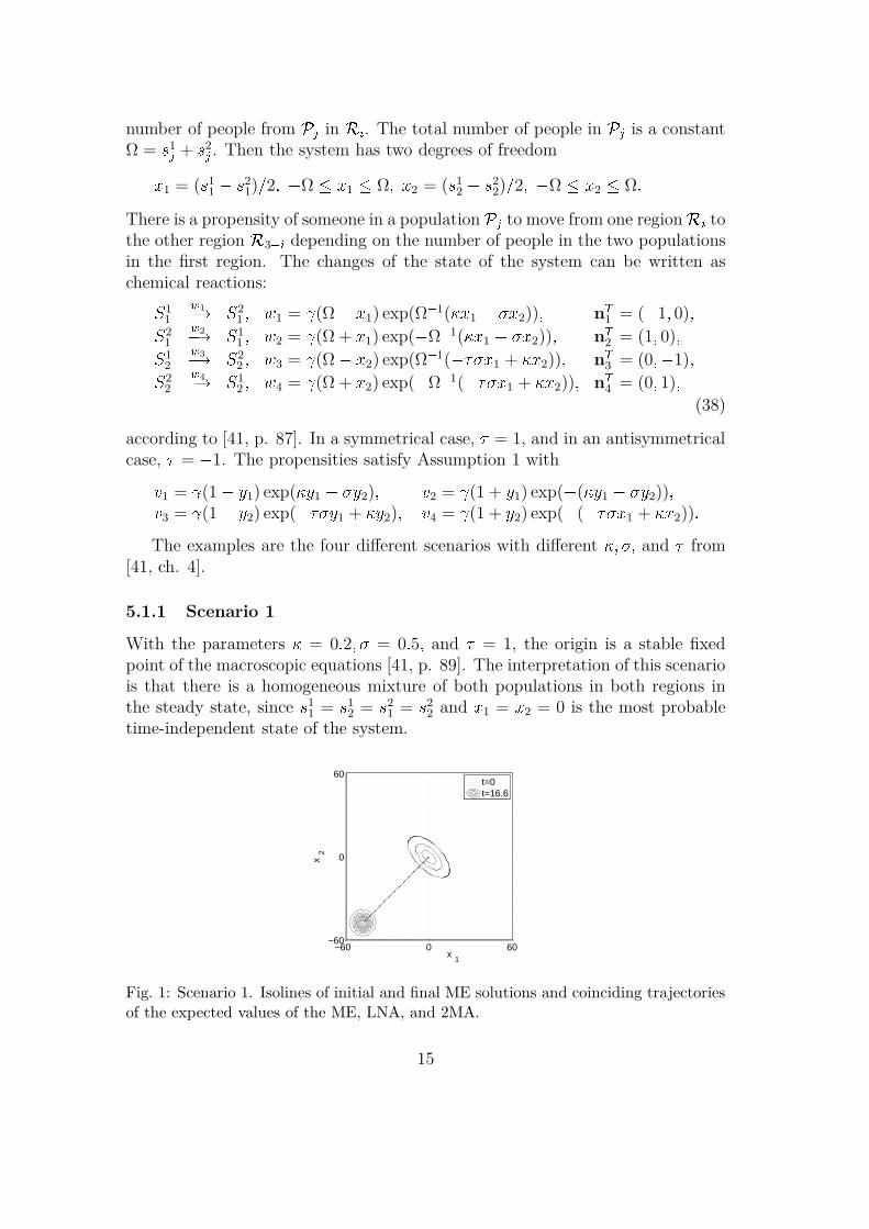
5.1.1 Scenario 1

With the parameters = 0:2; = 0:5; and = 1, the origin is a stable fixedpoint of the macroscopic equations [41, p. 89]. The interpretation of this scenariois that there is a homogeneous mixture of both populations in both regions inthe steady state, since s1

1 = s12 = s2

1 = s22 and x1 = x2 = 0 is the most probable

time-independent state of the system.

−60 0 60−60

0

60

x1

x2

t=0t=16.6

Fig. 1: Scenario 1. Isolines of initial and final ME solutions and coinciding trajectoriesof the expected values of the ME, LNA, and 2MA.

15

The master equation is solved with Ω = 60 in Figure 1 starting at t = 0 witha Gaussian distribution in the lower left corner. An approximate steady state atthe origin is reached at t = 16:6. The trajectories of the expected values from theME, LNA, and 2MA coincide when t 2 [0; 16:6] in this case and the covariancesare

(C11; C12; C22) =

8<: (59:6;36:8; 59:6) ME;(61:5;38:5; 61:5) LNA;(61:2;38:3; 61:2) 2MA:

The LNA and 2MA agree very well with the ME solution.

5.1.2 Scenario 2

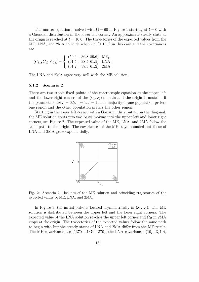
There are two stable fixed points of the macroscopic equation at the upper leftand the lower right corners of the (x1; x2)-domain and the origin is unstable ifthe parameters are = 0:5; = 1; = 1: The majority of one population prefersone region and the other population prefers the other region.

Starting in the lower left corner with a Gaussian distribution on the diagonal,the ME solution splits into two parts moving into the upper left and lower rightcorners, see Figure 2. The expected value of the ME, LNA, and 2MA follow thesame path to the origin. The covariances of the ME stays bounded but those ofLNA and 2MA grow exponentially.

−60 0 60−60

0

60

x1

x2

t=10t=0

Fig. 2: Scenario 2. Isolines of the ME solution and coinciding trajectories of theexpected values of ME, LNA, and 2MA.

In Figure 3, the initial pulse is located asymmetrically in (x1; x2). The MEsolution is distributed between the upper left and the lower right corners. Theexpected value of the LNA solution reaches the upper left corner and Ω in 2MAstops at the origin. The trajectories of the expected values follow the same pathto begin with but the steady states of LNA and 2MA differ from the ME result.The ME covariances are (1370;1370; 1370), the LNA covariances (10;3; 10),

16

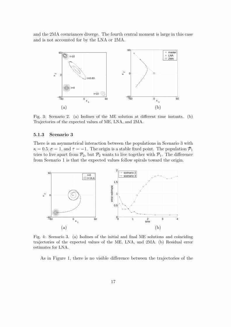
and the 2MA covariances diverge. The fourth central moment is large in this caseand is not accounted for by the LNA or 2MA.

−60 0 60−60

0

60

x1

x2

t=0

t=10

t=10

t=0.83

−60 0 60−60

0

60

x1

x2

masterLNA2MA

(a) (b)

Fig. 3: Scenario 2. (a) Isolines of the ME solution at different time instants. (b)Trajectories of the expected values of ME, LNA, and 2MA.

5.1.3 Scenario 3

There is an asymmetrical interaction between the populations in Scenario 3 with = 0:5; = 1; and = 1. The origin is a stable fixed point. The population P1

tries to live apart from P2, but P2 wants to live together with P1. The differencefrom Scenario 1 is that the expected values follow spirals toward the origin.

−60 0 60−60

0

60

x1

x2

t=0t=16.6

0 1 2 3 40

0.5

1

1.5

2

time

erro

r es

timat

e

scenario 2scenario 3

(a) (b)

Fig. 4: Scenario 3. (a) Isolines of the initial and final ME solutions and coincidingtrajectories of the expected values of the ME, LNA, and 2MA. (b) Residual errorestimates for LNA.

As in Figure 1, there is no visible difference between the trajectories of the

17

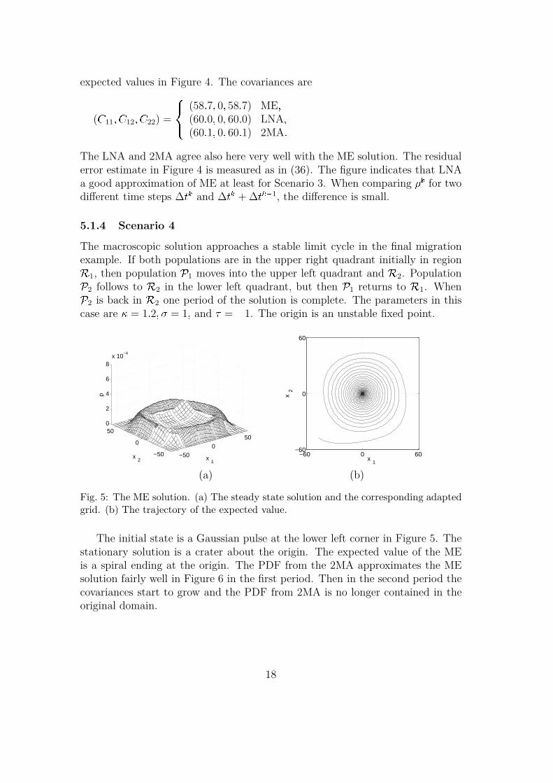
expected values in Figure 4. The covariances are

(C11; C12; C22) =

8<: (58:7; 0; 58:7) ME;(60:0; 0; 60:0) LNA;(60:1; 0; 60:1) 2MA:

The LNA and 2MA agree also here very well with the ME solution. The residualerror estimate in Figure 4 is measured as in (36). The figure indicates that LNAa good approximation of ME at least for Scenario 3. When comparing k for twodifferent time steps ∆tk and ∆tk + ∆tk1, the difference is small.

5.1.4 Scenario 4

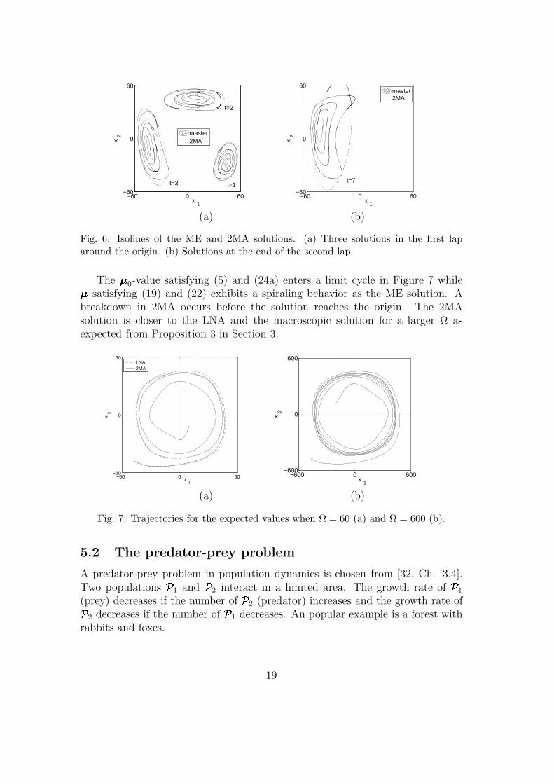
The macroscopic solution approaches a stable limit cycle in the final migrationexample. If both populations are in the upper right quadrant initially in regionR1, then population P1 moves into the upper left quadrant and R2. PopulationP2 follows to R2 in the lower left quadrant, but then P1 returns to R1. WhenP2 is back in R2 one period of the solution is complete. The parameters in thiscase are = 1:2; = 1; and = 1. The origin is an unstable fixed point.

−50

0

50

−50

0

500

2

4

6

8x 10

−4

x1

x2

p

−60 0 60−60

0

60

x1

x2

(a) (b)

Fig. 5: The ME solution. (a) The steady state solution and the corresponding adaptedgrid. (b) The trajectory of the expected value.

The initial state is a Gaussian pulse at the lower left corner in Figure 5. Thestationary solution is a crater about the origin. The expected value of the MEis a spiral ending at the origin. The PDF from the 2MA approximates the MEsolution fairly well in Figure 6 in the first period. Then in the second period thecovariances start to grow and the PDF from 2MA is no longer contained in theoriginal domain.

18

−60 0 60−60

0

60

x1

x2

t=1

t=2

t=3

master2MA

−60 0 60−60

0

60

x1

x2

t=7

master2MA

(a) (b)

Fig. 6: Isolines of the ME and 2MA solutions. (a) Three solutions in the first laparound the origin. (b) Solutions at the end of the second lap.

The 0-value satisfying (5) and (24a) enters a limit cycle in Figure 7 while satisfying (19) and (22) exhibits a spiraling behavior as the ME solution. Abreakdown in 2MA occurs before the solution reaches the origin. The 2MAsolution is closer to the LNA and the macroscopic solution for a larger Ω asexpected from Proposition 3 in Section 3.

−60 0 60−60

0

60

x1

x2

LNA2MA

−600 0 600−600

0

600

x1

x2

(a) (b)

Fig. 7: Trajectories for the expected values when Ω = 60 (a) and Ω = 600 (b).

5.2 The predator-prey problem

A predator-prey problem in population dynamics is chosen from [32, Ch. 3.4].Two populations P1 and P2 interact in a limited area. The growth rate of P1

(prey) decreases if the number of P2 (predator) increases and the growth rate ofP2 decreases if the number of P1 decreases. An popular example is a forest withrabbits and foxes.

19

The propensities for the macroscopic model in [32] satisfying Assumption 1are v1 = y1; v2 = y2

1 +ay1y2y1 + d; v3 = by2; v4 = by2

2y1

;with

nT1 = (1; 0); nT

2 = (1; 0); nT3 = (0;1); nT

4 = (0; 1):For some systems it is advantageous to introduce two scaling factors Ωi if the copynumbers xi differ in magnitude to keep yi of O(1). The theory in the previoussections covers the case when the scaling of the copy numbers is equal but thesolutions in the numerical experiments with Ω1=Ω2 = onst 6= 1 converge in thesame manner. Let x1 = Ω1y1 and x2 = Ω2y2. Then the propensities in the MEare written as chemical reactions:; w1! X1; w1 = Ω1v1(

x1

Ω1

; x2

Ω2

) = x1;X1w2! ;; w2 = Ω1v2(

x1

Ω1; x2

Ω2) =

x21

Ω1+

Ω1

Ω2

ax1x2x1 + Ω1d;; w3! X2; w3 = Ω2v3(x1

Ω1

; x2

Ω2

) = bx2;X2w4! ;; w4 = Ω2v4(

x1

Ω1; x2

Ω2) = bΩ1

Ω2

x22x1: (39)

The system is simulated with Ω2 = 0:5Ω1 and two different sets of parameters.The first macroscopic system has a stable fixed point and the second systemapproaches a stable limit cycle.

5.2.1 The stable system

The parameters in the first case are a = 0:75; b = 0:2; d = 0:2; in (39). The sizeparameter Ω1 is 200 in the first example.

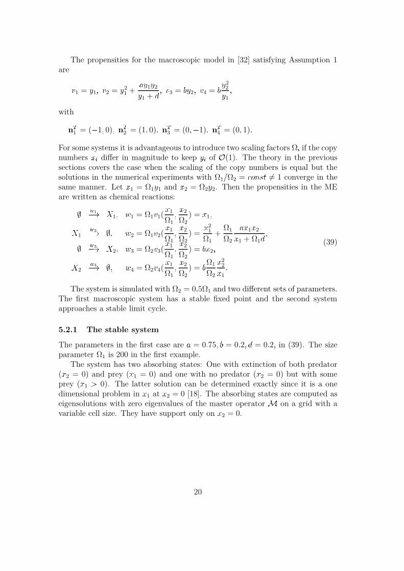
The system has two absorbing states: One with extinction of both predator(x2 = 0) and prey (x1 = 0) and one with no predator (x2 = 0) but with someprey (x1 > 0). The latter solution can be determined exactly since it is a onedimensional problem in x1 at x2 = 0 [18]. The absorbing states are computed aseigensolutions with zero eigenvalues of the master operator M on a grid with avariable cell size. They have support only on x2 = 0.

20

0 100 200 3000

0.2

0.4

0.6

0.8

1

p

x1

Fig. 8: Two eigensolutions corresponding to the eigenvalue zero.

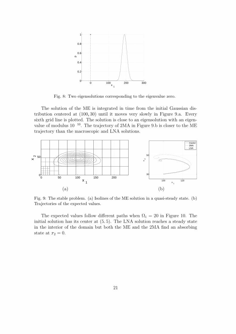
The solution of the ME is integrated in time from the initial Gaussian dis-tribution centered at (100; 30) until it moves very slowly in Figure 9.a. Everysixth grid line is plotted. The solution is close to an eigensolution with an eigen-value of modulus 1010. The trajectory of 2MA in Figure 9.b is closer to the MEtrajectory than the macroscopic and LNA solutions.

0 50 100 150 2000

50

x1

x2

100 120

30

50

x1

x2

master2MALNA

(a) (b)

Fig. 9: The stable problem. (a) Isolines of the ME solution in a quasi-steady state. (b)Trajectories of the expected values.

The expected values follow different paths when Ω1 = 20 in Figure 10. Theinitial solution has its center at (5; 5). The LNA solution reaches a steady statein the interior of the domain but both the ME and the 2MA find an absorbingstate at x2 = 0.

21

0 5 10 150

5

x1

x2

masterLNA2MA

Fig. 10: Trajectories the expected values of the stable problem.

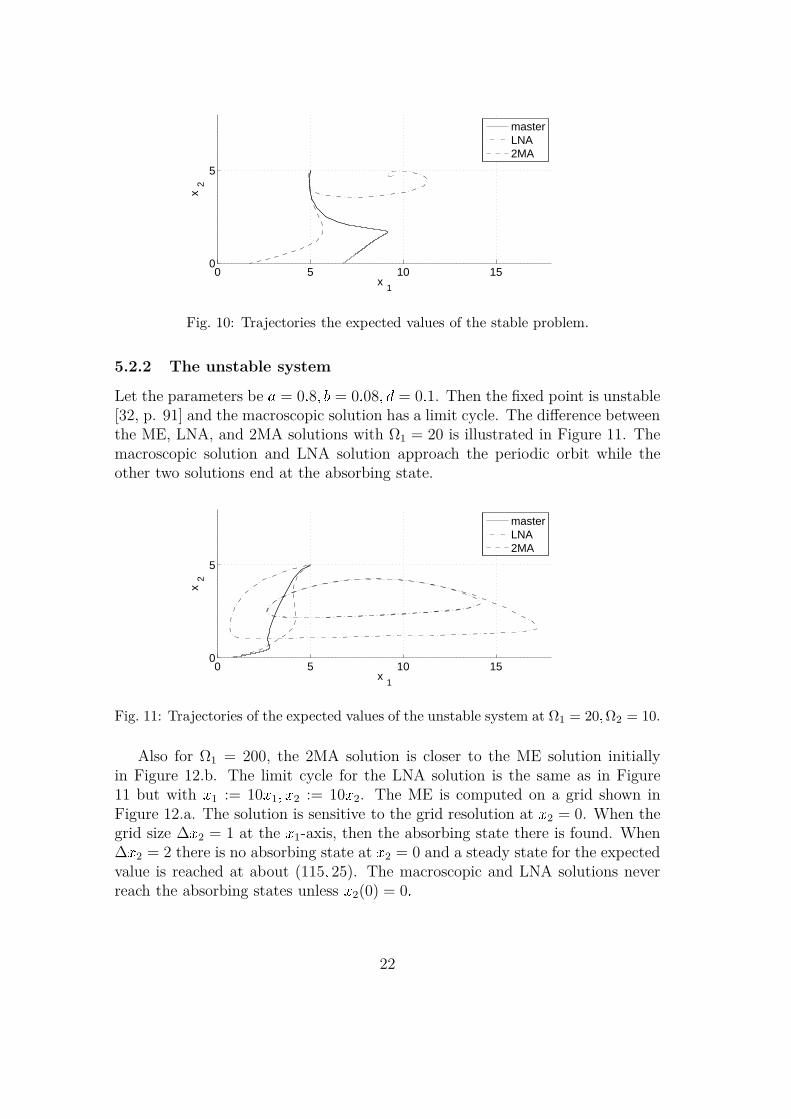
5.2.2 The unstable system

Let the parameters be a = 0:8; b = 0:08; d = 0:1. Then the fixed point is unstable[32, p. 91] and the macroscopic solution has a limit cycle. The difference betweenthe ME, LNA, and 2MA solutions with Ω1 = 20 is illustrated in Figure 11. Themacroscopic solution and LNA solution approach the periodic orbit while theother two solutions end at the absorbing state.

0 5 10 150

5

x1

x2

masterLNA2MA

Fig. 11: Trajectories of the expected values of the unstable system at Ω1 = 20;Ω2 = 10.

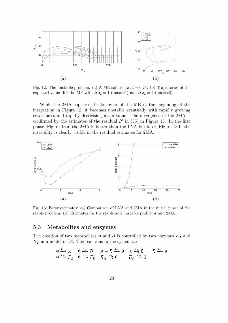
Also for Ω1 = 200, the 2MA solution is closer to the ME solution initiallyin Figure 12.b. The limit cycle for the LNA solution is the same as in Figure11 but with x1 := 10x1; x2 := 10x2. The ME is computed on a grid shown inFigure 12.a. The solution is sensitive to the grid resolution at x2 = 0. When thegrid size ∆x2 = 1 at the x1-axis, then the absorbing state there is found. When∆x2 = 2 there is no absorbing state at x2 = 0 and a steady state for the expectedvalue is reached at about (115; 25). The macroscopic and LNA solutions neverreach the absorbing states unless x2(0) = 0:

22

0 100 2000

25

50

75

x1

x2

80 90 100 110 120 13020

25

30

35

40

x1

x2

master1master22MALNA

(a) (b)

Fig. 12: The unstable problem. (a) A ME solution at t = 6:25. (b) Trajectories of theexpected values for the ME with ∆x2 = 1 (master1) and ∆x2 = 2 (master2).

While the 2MA captures the behavior of the ME in the beginning of theintegration in Figure 12, it becomes unstable eventually with rapidly growingcovariances and rapidly decreasing mean value. The divergence of the 2MA isconfirmed by the estimates of the residual k in (36) in Figure 13. In the firstphase, Figure 13.a, the 2MA is better than the LNA but later, Figure 13.b, theinstability is clearly visible in the residual estimates for 2MA.

0 2 4 6

0.2

0.4

time

erro

r es

timat

e

LNA2MA

0 5 10 15 20 250

2

4

6

8

time

erro

r es

timat

e

unstablestable

(a) (b)

Fig. 13: Error estimates: (a) Comparison of LNA and 2MA in the initial phase of thestable problem. (b) Estimates for the stable and unstable problems and 2MA.

5.3 Metabolites and enzymes

The creation of two metabolites A and B is controlled by two enzymes EA andEB in a model in [8]. The reactions in the system are; w1! A ; w2! B A + B w3! ; A w4! ; B w5! ;; w6! EA ; w7! EB EA w8! ; EB w9! ;23

The propensities in the master equation for the nine reactions and the speciesxT = (a; b; eA; eB) are

nT1 = (1; 0; 0; 0); w1 = Ω

kAeAΩ + aKI ; nT

2 = (0;1; 0; 0); w2 = ΩkBeB

Ω + bKI ;nT

3 = (1; 1; 0; 0); w3 = k2Ω1ab; nT

4 = (1; 0; 0; 0); w4 = a;nT

5 = (0; 1; 0; 0); w5 = b; nT6 = (0; 0;1; 0); w6 = Ω

kEAΩ + aKR ;

nT7 = (0; 0; 0;1); w7 = Ω

kEBΩ + bKR ; nT

8 = (0; 0; 1; 0); w8 = eA;nT

9 = (0; 0; 0; 1); w9 = eB:(40)

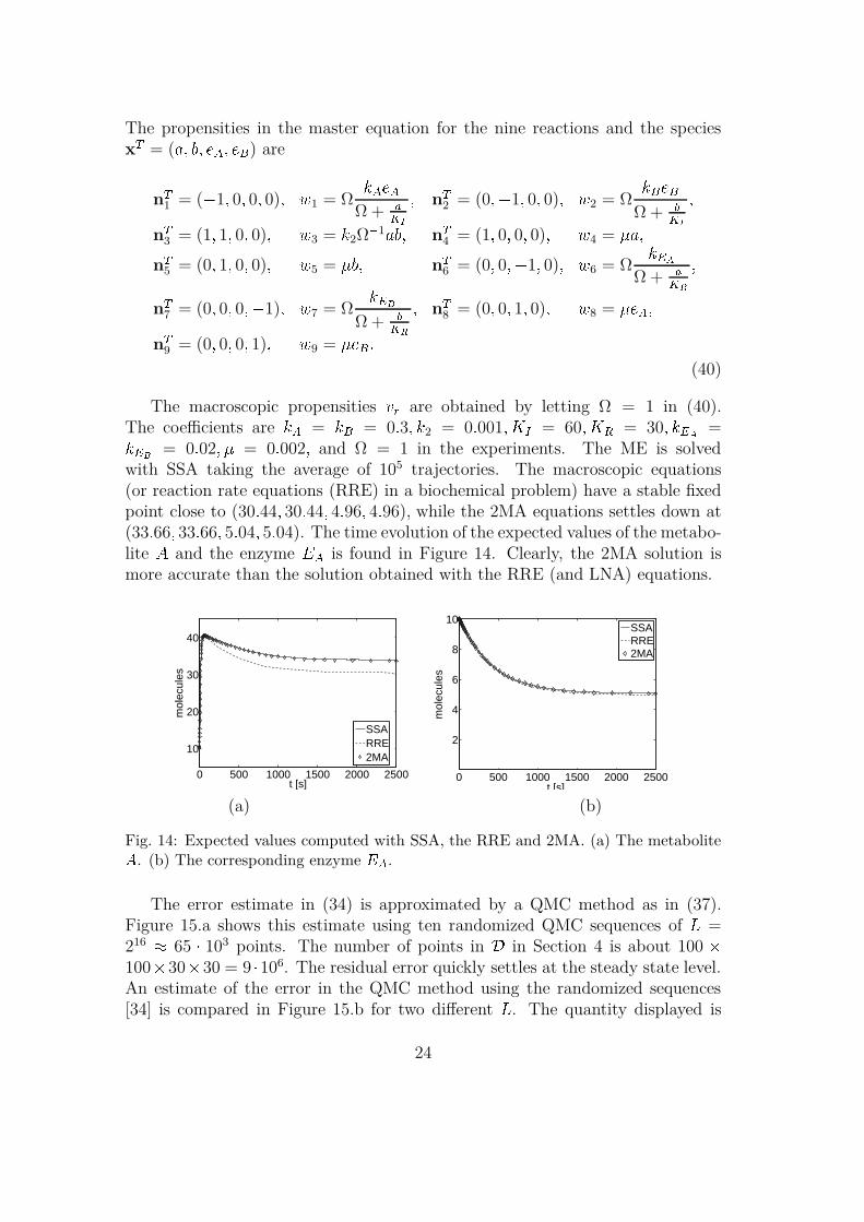
The macroscopic propensities vr are obtained by letting Ω = 1 in (40).The coefficients are kA = kB = 0:3; k2 = 0:001; KI = 60; KR = 30; kEA =kEB = 0:02; = 0:002; and Ω = 1 in the experiments. The ME is solvedwith SSA taking the average of 105 trajectories. The macroscopic equations(or reaction rate equations (RRE) in a biochemical problem) have a stable fixedpoint close to (30:44; 30:44; 4:96; 4:96), while the 2MA equations settles down at(33:66; 33:66; 5:04; 5:04). The time evolution of the expected values of the metabo-lite A and the enzyme EA is found in Figure 14. Clearly, the 2MA solution ismore accurate than the solution obtained with the RRE (and LNA) equations.

0 500 1000 1500 2000 2500

10

20

30

40

t [s]

mol

ecul

es

SSARRE2MA

0 500 1000 1500 2000 2500

2

4

6

8

10

t [s]

mol

ecul

es

SSARRE2MA

(a) (b)

Fig. 14: Expected values computed with SSA, the RRE and 2MA. (a) The metaboliteA. (b) The corresponding enzyme EA.

The error estimate in (34) is approximated by a QMC method as in (37).Figure 15.a shows this estimate using ten randomized QMC sequences of L =216 65 103 points. The number of points in D in Section 4 is about 100 1003030 = 9 106. The residual error quickly settles at the steady state level.An estimate of the error in the QMC method using the randomized sequences[34] is compared in Figure 15.b for two different L. The quantity displayed is

24

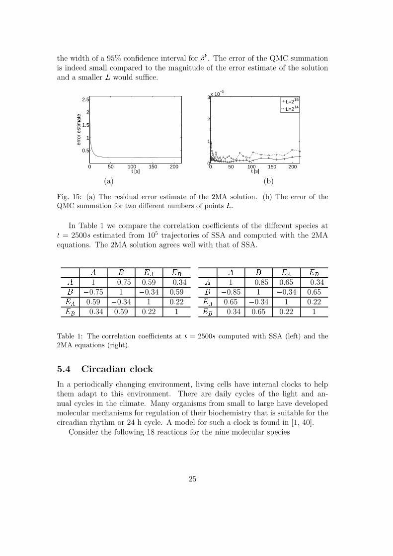
the width of a 95% confidence interval for k. The error of the QMC summationis indeed small compared to the magnitude of the error estimate of the solutionand a smaller L would suffice.

0 50 100 150 200

0.5

1

1.5

2

2.5

t [s]

erro

r es

timat

e

0 50 100 150 2000

1

2

3x 10

−3

t [s]

L=216

L=214

(a) (b)

Fig. 15: (a) The residual error estimate of the 2MA solution. (b) The error of theQMC summation for two different numbers of points L.

In Table 1 we compare the correlation coefficients of the different species att = 2500s estimated from 105 trajectories of SSA and computed with the 2MAequations. The 2MA solution agrees well with that of SSA.A B EA EBA 1 0:75 0:59 0:34B 0:75 1 0:34 0:59EA 0:59 0:34 1 0:22EB 0:34 0:59 0:22 1

A B EA EBA 1 0:85 0:65 0:34B 0:85 1 0:34 0:65EA 0:65 0:34 1 0:22EB 0:34 0:65 0:22 1

Table 1: The correlation coefficients at t = 2500s computed with SSA (left) and the2MA equations (right).

5.4 Circadian clock

In a periodically changing environment, living cells have internal clocks to helpthem adapt to this environment. There are daily cycles of the light and an-nual cycles in the climate. Many organisms from small to large have developedmolecular mechanisms for regulation of their biochemistry that is suitable for thecircadian rhythm or 24 h cycle. A model for such a clock is found in [1, 40].

Consider the following 18 reactions for the nine molecular species

25

A;C;R;Da; D0a; Dr; D0r;Ma;M 0a modeling the circadian rhythm in [1]:D0a aD0a! DaDa + A aDaA! D0aD0r rD0r! DrDr + A rDrA! D0r9>>>>=>>>>; ; 0aD0a! Ma; aDa! MaMa ÆmaMa! ; 9>=>; ; aMa! A; aD0a! A; rD0r! AA ÆaA! ;A + R AR! C

9>>>>>>>=>>>>>>>;; 0rD0r! Mr; rDr! MrMr ÆmrMr! ; 9>=>; ; rMr! RR ÆrR! ;C ÆaC! R 9>=>; (41)

All propensities vr are linear in the species except for three reactions with aquadratic dependence in (41). The corresponding wr-form is the same as abovefor a linear vr and divided by Ω for a quadratic vr.

The reaction constants are found in Table 2. The parameter Ær will havevalues between 0 and 0:2 in the numerical experiments. The initial conditionsare zero for all variables except for Da(0) = Dr(0) = 1.a 50 a 50 a 1 Æma 10 a 500a 500 r 5 r 1 Æmr 0.5 r 100r 0.01 2 Æa 10r 50 Ær -

Table 2: Parameters of the circadian clock.

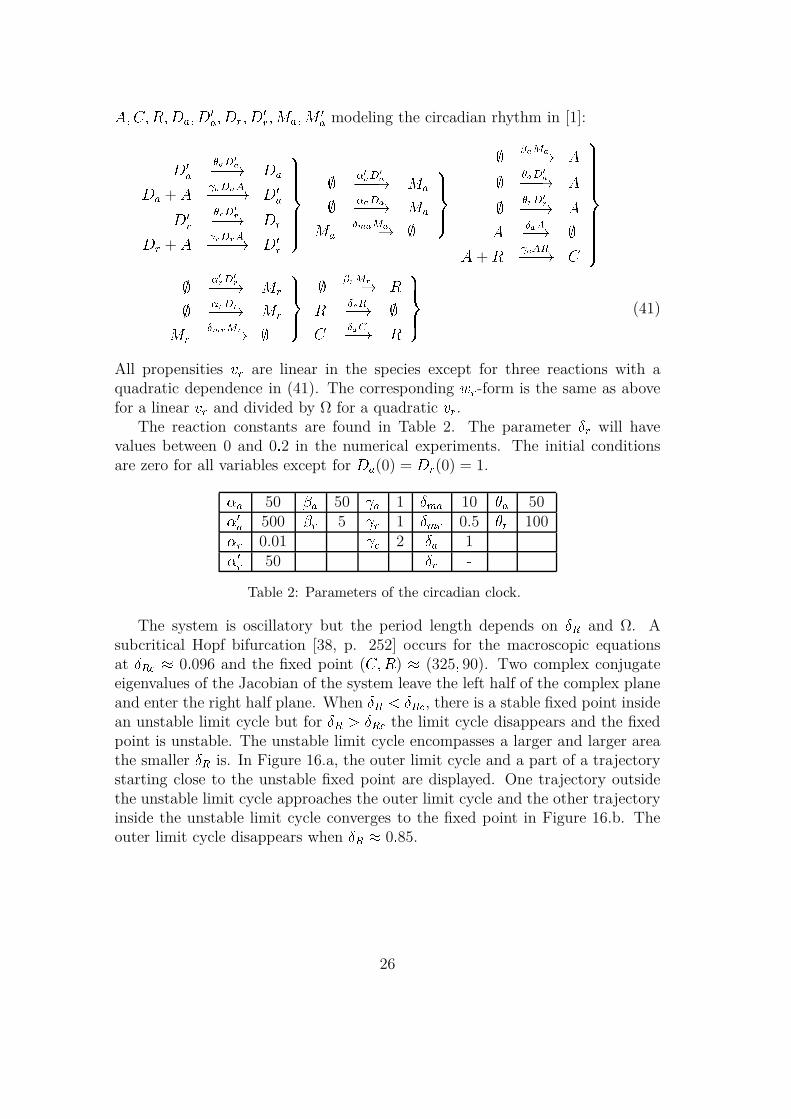
The system is oscillatory but the period length depends on ÆR and Ω. Asubcritical Hopf bifurcation [38, p. 252] occurs for the macroscopic equationsat ÆR 0:096 and the fixed point (C;R) (325; 90). Two complex conjugateeigenvalues of the Jacobian of the system leave the left half of the complex planeand enter the right half plane. When ÆR < ÆR , there is a stable fixed point insidean unstable limit cycle but for ÆR > ÆR the limit cycle disappears and the fixedpoint is unstable. The unstable limit cycle encompasses a larger and larger areathe smaller ÆR is. In Figure 16.a, the outer limit cycle and a part of a trajectorystarting close to the unstable fixed point are displayed. One trajectory outsidethe unstable limit cycle approaches the outer limit cycle and the other trajectoryinside the unstable limit cycle converges to the fixed point in Figure 16.b. Theouter limit cycle disappears when ÆR 0:85.

26

0 500 1000 1500 20000

500

1000

1500

2000

C

R

300 325 350

75

100

125

C

R

(a) (b)

Fig. 16: (a) The outer limit cycle and the unstable fixed point at (C;R) (325; 90) forÆR = 0:097. (b) A close-up view of the stable fixed point and the unstable limit cyclefor ÆR = 0:095.

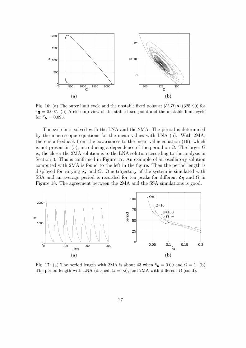
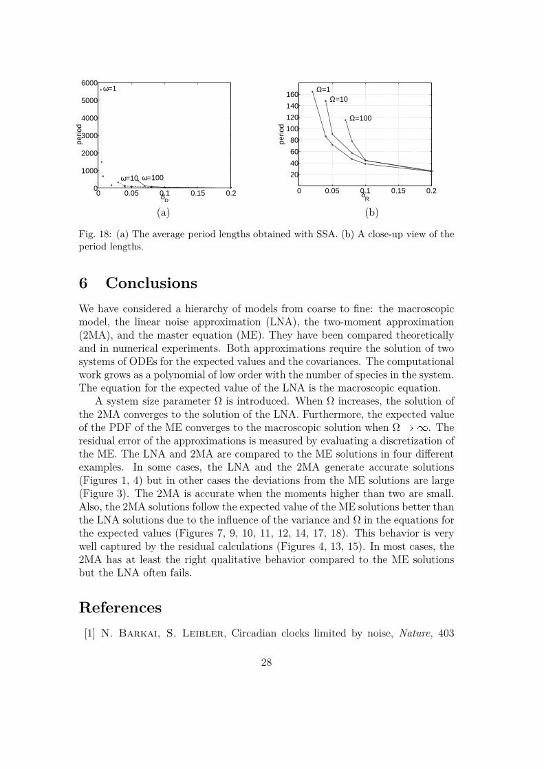
The system is solved with the LNA and the 2MA. The period is determinedby the macroscopic equations for the mean values with LNA (5). With 2MA,there is a feedback from the covariances to the mean value equation (19), whichis not present in (5), introducing a dependence of the period on Ω. The larger Ωis, the closer the 2MA solution is to the LNA solution according to the analysis inSection 3. This is confirmed in Figure 17. An example of an oscillatory solutioncomputed with 2MA is found to the left in the figure. Then the period length isdisplayed for varying ÆR and Ω. One trajectory of the system is simulated withSSA and an average period is recorded for ten peaks for different ÆR and Ω inFigure 18. The agreement between the 2MA and the SSA simulations is good.

0 100 200 3000

1000

2000

time

R

0.05 0.1 0.15 0.20

25

50

75

100

Ω=∞

Ω=1

Ω=10

Ω=100

δR

perio

d

(a) (b)

Fig. 17: (a) The period length with 2MA is about 43 when ÆR = 0:09 and Ω = 1. (b)The period length with LNA (dashed, Ω =1), and 2MA with different Ω (solid).

27

0 0.05 0.1 0.15 0.20

1000

2000

3000

4000

5000

6000

δR

perio

d

ω=100ω=10

ω=1

0 0.05 0.1 0.15 0.2

20

40

60

80

100

120

140

160

δR

perio

d

Ω=1Ω=10

Ω=100

(a) (b)

Fig. 18: (a) The average period lengths obtained with SSA. (b) A close-up view of theperiod lengths.

6 Conclusions

We have considered a hierarchy of models from coarse to fine: the macroscopicmodel, the linear noise approximation (LNA), the two-moment approximation(2MA), and the master equation (ME). They have been compared theoreticallyand in numerical experiments. Both approximations require the solution of twosystems of ODEs for the expected values and the covariances. The computationalwork grows as a polynomial of low order with the number of species in the system.The equation for the expected value of the LNA is the macroscopic equation.

A system size parameter Ω is introduced. When Ω increases, the solution ofthe 2MA converges to the solution of the LNA. Furthermore, the expected valueof the PDF of the ME converges to the macroscopic solution when Ω !1. Theresidual error of the approximations is measured by evaluating a discretization ofthe ME. The LNA and 2MA are compared to the ME solutions in four differentexamples. In some cases, the LNA and the 2MA generate accurate solutions(Figures 1, 4) but in other cases the deviations from the ME solutions are large(Figure 3). The 2MA is accurate when the moments higher than two are small.Also, the 2MA solutions follow the expected value of the ME solutions better thanthe LNA solutions due to the influence of the variance and Ω in the equations forthe expected values (Figures 7, 9, 10, 11, 12, 14, 17, 18). This behavior is verywell captured by the residual calculations (Figures 4, 13, 15). In most cases, the2MA has at least the right qualitative behavior compared to the ME solutionsbut the LNA often fails.

References

[1] N. Barkai, S. Leibler, Circadian clocks limited by noise, Nature, 403

28

(2000), p. 267–268.

[2] R. E. Caflisch, Monte Carlo and quasi-Monte Carlo methods, Acta Nu-merica, 1998, p. 1–49.

[3] Y. Cao, D. Gillespie, L. Petzold, Multiscale stochastic simulationalgorithm with stochastic partial equilibrium assumption for chemically re-acting systems, J. Comput. Phys., 206 (2005), p. 395–411.

[4] W.-Y. Chen, A. Bokka, Stochastic modeling of nonlinear epidemiology,J. Theor. Biol., 234 (2005), p. 455–470.

[5] U. Dieckmann, P. Marrow, R. Law, Evolutionary cycling in predator-prey interactions: Population dynamics and the Red Queen, J. Theor. Biol.,176 (1995), p. 91–102.

[6] J. Dieudonne, Foundations of Modern Analysis, Academic Press, NewYork, 1969.

[7] W. E, D. Liu, E. Vanden-Eijnden, Nested stochastic simulation algo-rithm for chemical kinetic systems with multiple time scales, J. Comput.Phys., 221 (2007), p. 158–180.

[8] J. Elf, P. Lotstedt, P. Sjoberg, Problems of high di-mension in molecular biology, in High-dimensional problems - Nu-merical treatment and applications, ed. W. Hackbusch, Proceedingsof the 19th GAMM-Seminar Leipzig 2003, p. 21-30, available athttp://www.mis.mpg.de/conferences/gamm/2003/.

[9] J. Elf, M. Ehrenberg, Fast evaluation of fluctuations in biochemicalnetworks with the linear noise approximation, Genome Res., 13 (2003), p.2475–2484.

[10] J. Elf, J. Paulsson, O. G. Berg, M. Ehrenberg, Near-critical phe-nomena in intracellular metabolite pools, Biophys. J., 84 (2003), p. 154–170.

[11] C. Escudera, J. Buceta, F. J. de la Rubia, K. Lindenberg, Ex-tinction in population dynamics, Phys. Rev. E, 69 (2004), 021908.

[12] S. Engblom, Computing the moments of high dimensional solutions of themaster equation, Appl. Math. Comput., 180 (2006), p. 498–515.

[13] B. Engquist, O. Runborg, Computational high frequency wave propa-gation, Acta Numerica, (2003), p. 181–266.

[14] S. N. Ethier, T. G. Kurtz, Markov Processes, Characterization andConvergence, John Wiley, New York, 1986.

29

[15] H. Faure, Discrepance de suites associees a un systeme de numeration (endimension s), Acta Aritm., 41 (1982), p. 337–351.

[16] L. Ferm, P. Lotstedt, P. Sjoberg, Conservative solution of the Fokker-Planck equation for stochastic chemical reactions, BIT, 46 (2006), p. S61–S83.

[17] R. F. Fox, J. Keizer, Amplification of intrinsic fluctuations by chaoticdynamics in physical systems, Phys. Rev. A, 43 (1991), p. 1709–1720.

[18] C. W. Gardiner, Handbook of Stochastic Methods, 3rd ed., Springer,Berlin, 2004.

[19] M. B. Giles and E. Suli, Adjoint methods for PDEs: a posteriori erroranalysis and postprocessing by duality, Acta Numerica, 11 (2002), p. 145–236.

[20] D. T. Gillespie, A general method for numerically simulating the stochas-tic time evolution of coupled chemical reactions, J. Comput. Phys., 22 (1976),p. 403–434.

[21] D. Givon, R. Kupferman, A. Stewart, Extracting macroscopic dynam-ics: model problems and algorithms, Nonlinearity, 17 (2004), p. R55–R127.

[22] E. Hairer, S. P. Nørsett, G. Wanner, Solving Ordinary DifferentialEquations I, Nonstiff Problems, 2nd ed., Springer-Verlag, Berlin, 1993.

[23] H. S. Hong, F. J. Hickernell, Algorithm 823: Implementing scrambleddigital sequences, ACM Trans. Math. Softw., 29 (2003), p. 95–109.

[24] N. G. van Kampen, The expansion of the master equation, Adv. Chem.Phys., 34 (1976), p. 245–309.

[25] N. G. van Kampen, Stochastic Processes in Physics and Chemistry, North-Holland, Amsterdam, 1992.

[26] T. G. Kurtz, Solutions of ordinary differential equations as limits of purejump Markov processes, J. Appl. Probab., 7 (1970), p. 49–58.

[27] T. G. Kurtz, Limit theorems for sequences of jump Markov processesapproximating ordinary differential processes, J. Appl. Probab., 7 (1971), p.344–356.

[28] P. Lotstedt, L. Ferm, Dimensional reduction of the Fokker-Planck equa-tion for stochastic chemical reactions, Multiscale Meth. Simul., 5 (2006), p.593–614.

30

[29] H. H. McAdams, A. Arkin, Stochastic mechanisms in gene expression,Proc. Natl. Acad. Sci. USA, 94 (1997), p. 814–819.

[30] H. H. McAdams, A. Arkin, It’s a noisy business. Genetic regulation atthe nanomolar scale, Trends Gen., 15 (1999), p. 65–69.

[31] A. J. McKane, T. J. Newman, Stochastic models in population biologyand their deterministic analogs, Phys. Rev. E, 70 (2004), 041902.

[32] J. D. Murray, Mathematical Biology. I: An Introduction, 3rd ed., Springer,New York, 2002.

[33] J. T. Oden, S. Prudhomme, Estimation of modeling error in computa-tional mechanics, J. Comput. Phys., 182 (2002), p. 496–515.

[34] A. B. Owen, Monte Carlo variance of scrambled net quadrature, SIAM J.Numer. Anal., 34 (1997), p. 1884–1910.

[35] H. Risken, The Fokker-Planck Equation, 2nd ed., Springer, Berlin, 1996.

[36] P. Sjoberg, P. Lotstedt, J. Elf, Fokker-Planck approxima-tion of the master equation in molecular biology, Technical report2005-044, Dept of Information Technology, Uppsala University, Up-psala, Sweden, 2005, to appear in Comput. Vis. Sci., available athttp://www.it.uu.se/research/reports/2005-044/.

[37] N. Stollenwerk, V. A. A. Jensen, Meningitis, pathogenicity near crit-icality: the epidemiology of meningococcal disease as a model for accidentalpathogens, J. Theor. Biol., 222 (2003), p. 347–359.

[38] S. H. Strogatz, Nonlinear Dynamics and Chaos, Perseus Books, Cam-bridge, MA, 1994.

[39] S. Succi, The Lattice Boltzmann Equation for Fluid Dynamics and Beyond,Clarendon Press, Oxford, 2001.

[40] J. M. G. Vilar, H. Y. Kueh, N. Barkai, S. Leibler, Mechanisms ofnoise-resistance in genetic oscillators, Proc. Nat. Acad. Sci. USA, 99 (2002),p. 5988–5992.

[41] W. Weidlich, Sociodynamics. A Systematic Approach to MathematicalModelling in the Social Sciences, Taylor and Francis, London, 2000.

[42] W. Weidlich, Thirty years of sociodynamics. An integrated strategy ofmodelling in the social sciences: applications to migration and urban evolu-tion, Chaos, Solit. Fract., 24 (2005), p. 45–56.

[43] D. C. Wilcox, Turbulence Modeling for CFD, DCW Industries, Inc., LaCanada, CA, 1994.

31