A Hierarchical Conditional Random Field Model for … Hierarchical Conditional Random Field Model for Labeling and Segmenting Images of Street Scenes Qixing Huang Stanford University

A Hierarchical Conditional Random Field Model for Labeling and SegmentingImages of Street Scenes

Qixing HuangStanford University

[email protected]

Mei HanGoogle Inc.

[email protected]

Bo WuGoogle Inc.

[email protected]

Sergey IoffeGoogle Inc.

[email protected]

Abstract

Simultaneously segmenting and labeling images is a fun-damental problem in Computer Vision. In this paper, weintroduce a hierarchical CRF model to deal with the prob-lem of labeling images of street scenes by several distinc-tive object classes. In addition to learning a CRF modelfrom all the labeled images, we group images into clustersof similar images and learn a CRF model from each clusterseparately. When labeling a new image, we pick the closestcluster and use the associated CRF model to label this im-age. Experimental results show that this hierarchical imagelabeling method is comparable to, and in many cases supe-rior to, previous methods on benchmark data sets. In addi-tion to segmentation and labeling results, we also showedhow to apply the image labeling result to rerank Googlesimilar images.

1. Introduction

Simultaneous segmenting and labeling images is a fun-damental problem in computer vision. It is the core tech-nology of image understanding, content based retrieval andobject recognition. The goal is to assign every pixel of theimage with an object class label. Most solutions fall intotwo general categories: parametric methods and nonpara-metric methods.

Parametric methods [2, 4, 7, 12, 14, 17, 18] usually in-volve optimizing a Conditional Random Field (CRF) modelwhich evaluates the probability of assigning a particular la-bel to each pixel, and the probability of assigning each pairof labels to neighboring pixels. A parametric method usu-ally has a learning phase where the parameters of the CRFmodels are optimized from training examples, and an infer-ence phase where the CRF model is applied to label a testimage.

In contrast to parametric methods, nonparametric meth-ods [10, 15] do not involve any training at all. The basicidea of these methods is to transfer labels from a retrieval

set which contains semantically similar images. Nonpara-metric methods tend to be more scalable than parametricmethods because it is easy for nonparametric methods toincorporate new training examples and class labels.

In this paper, we introduce a hierarchical two-stage CRFmodel which combines the ideas used in both parametricand nonparametric image labeling methods. In addition tolearning a global CRF model from all the training images,we group training data into clusters of images with similarspatial object class layout and object appearance, and train aseparate CRF model for each cluster. Given a test image, wefirst run the global CRF model to obtain initial pixel labels.We then find the cluster with most similar images, as shownin Fig. 1. Finally, we relabel the input image by the CRFmodel associated with this cluster. To effectively compareand extract similar images, we introduce a new image de-scriptor: the label-based descriptor which summarizes thesemantic information of a labeled image.

Our approach is motivated by the emergence of largedata sets of labeled images, such as Labelme data set [13].The Labelme data set contains tens of thousands of labeledimages. It provides sufficient instances to train classifiersfor each type of images with similar spatial layout. In thispaper, we focus on images of street scenes which are themost dominant ones in Labelme data set. However, there isno restriction on extending our approach to handling othertypes of images if more training data is available.

Experimental results show that the hierarchical two-stage CRF model is superior to the global CRF modellearned from all training examples. Evaluations on bench-mark data sets demonstrate that our approach is comparable,and in many cases, superior to state-of-the-art parametricand nonparametric approaches. In addition, we also showpromising results of applying the label-based descriptor tocompute images of similar spatial layout and re-rank similarimage results from Google Image Search.

1.1. Related Work

Parametric methods. Image labeling by optimizing aCRF model has proven to be the state-of-the-art paramet-

1953

Figure 1: The pipeline of our hierarchical two-stage CRF model. Given a test image, we first run the global CRF modeltrained by all training images to obtain initial pixel labels. Based on these pixel labels, we compute the label-based descriptorto find the closest image cluster. Finally, we relabel the test image using the CRF model associated with this cluster.

ric image labeling method. Traditional CRF models [4, 14]combine unary energy terms, which evaluate the possibilityof a single pixel taking a particular label, and pair-wise en-ergy terms, which evaluate the probability of adjacent pix-els taking different labels. Although these approaches workwell in many cases, they still have their own limitations be-cause these CRF models are only up to second-order andit is difficult to incorporate large-scale contextual informa-tion.

Many researchers have considered variants of traditionalCRF models to improve their performance. In [6], Kohli etal. proposed to use higher order potentials for improving thelabeling consistency. Another line of research focuses onexploring the object class co-occurrence [2, 7, 12, 17, 18].In particular, Ladicky et al. [7] introduced a co-occurrencemodel that can be efficiently optimized using graph-cuts.

Our approach also falls into the category of paramet-ric image labeling methods, but it has notable differencesfrom previous approaches. Instead of improving the CRFmodel used in labeling, we try to divide training images intogroups of visually and semantically similar images such thattraditional CRF models could have better fits on each ofthem. Note that learning CRF models from clusters of sim-ilar images implicitly includes high-level statistics such ashigh-order potentials and object class co-occurrence.Nonparametric methods. The key components of non-parametric methods are how to find the retrieval set whichcontains similar images, and how to build pixel-wise orsuperpixel-wise links between the input image and imagesin the retrieval set. In [10], Liu et al. introduced SIFTFlow to establish pixel-wise links. Since SIFT Flow worksbest when the retrieval set images are highly similar to theinput image in spatial layout of object classes, Tighe andLazebnik introduced a scalable approach that allows morevariation between the layout of the input image and imagesin the retrieval set [15]. Moreover, both methods utilize aMRF model to obtain the final labeling result. The differ-ence is that the approach of [15] works at super-pixel levelwhich turns out to be more efficient than the approach of[10] which is pixel-wised.

Like most nonparametric methods, our approach also ex-tracts information from images with similar spatial layout

of object classes and object appearances. However, the fun-damental difference is that we pre-compute classifiers forgroups of similar images. This gives us freedom in design-ing suitable classifiers at the learning phase and saves theinference time.

2. Image Labeling Using Standard CRF

In this section, we describe the CRF model used for la-beling images of street scenes. This CRF model serves asthe building block for the hierarchical CRF model to be in-troduced in next Section. Our CRF model is similar to theones used in [4] and [14]. However, we use different fea-tures for both the unary and pair-wise potentials which aremore suitable for images of street scenes.

As there are many different objects in street scene im-ages, it is quite challenging to classify all of them. In thispaper, we choose five distinctive super-classes: sky, archi-tecture, plant, road and misc. Each super-class contains sev-eral different objects. Please refer to Table 1 for details.

super-classes objectssky sky, cloud

architecture building, wall, hill, bridge, · · ·plant tree, grass, flower,· · ·

ground road, street, sidewalk, water, earth,· · ·misc people, car, animal, bicycle, · · ·

Table 1: Objects in each super-class.

The motivation of introducing super-classes is three-fold. First, the position, shape and appearance of these fivesuper-classes primarily determine the semantic informationof a street scene image. Second, maintaining a small set ofsuper-classes reduces the training time which, on the otherhand, enables us to incorporate more information for clas-sification. Third, if necessary, one can still apply anotherlayer of other classification method to distinguish the ob-jects within each super-class.

The training and testing images used in this paper comefrom the Labelme data set [13]. We manually collect allthe labeled images that were taken outdoor and contain atleast two labels from the set of sky, building, tree, street. As

1954

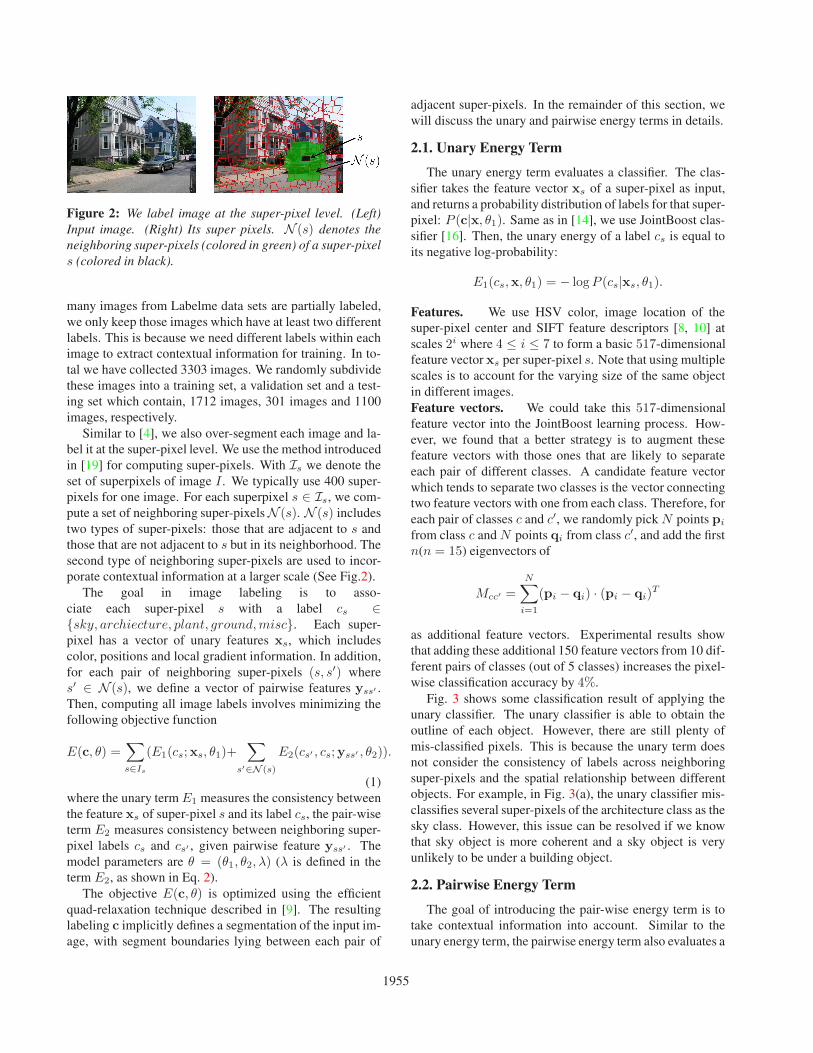
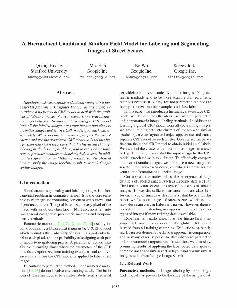
Figure 2: We label image at the super-pixel level. (Left)Input image. (Right) Its super pixels. N (s) denotes theneighboring super-pixels (colored in green) of a super-pixels (colored in black).

many images from Labelme data sets are partially labeled,we only keep those images which have at least two differentlabels. This is because we need different labels within eachimage to extract contextual information for training. In to-tal we have collected 3303 images. We randomly subdividethese images into a training set, a validation set and a test-ing set which contain, 1712 images, 301 images and 1100images, respectively.

Similar to [4], we also over-segment each image and la-bel it at the super-pixel level. We use the method introducedin [19] for computing super-pixels. With Is we denote theset of superpixels of image I . We typically use 400 super-pixels for one image. For each superpixel s ∈ Is, we com-pute a set of neighboring super-pixels N (s). N (s) includestwo types of super-pixels: those that are adjacent to s andthose that are not adjacent to s but in its neighborhood. Thesecond type of neighboring super-pixels are used to incor-porate contextual information at a larger scale (See Fig.2).

The goal in image labeling is to asso-ciate each super-pixel s with a label cs ∈{sky, archiecture, plant, ground,misc}. Each super-pixel has a vector of unary features xs, which includescolor, positions and local gradient information. In addition,for each pair of neighboring super-pixels (s, s′) wheres′ ∈ N (s), we define a vector of pairwise features yss′ .Then, computing all image labels involves minimizing thefollowing objective function

E(c, θ) =∑

s∈Is

(E1(cs;xs, θ1)+∑

s′∈N (s)

E2(cs′ , cs;yss′ , θ2)).

(1)where the unary term E1 measures the consistency betweenthe feature xs of super-pixel s and its label cs, the pair-wiseterm E2 measures consistency between neighboring super-pixel labels cs and cs′ , given pairwise feature yss′ . Themodel parameters are θ = (θ1, θ2, λ) (λ is defined in theterm E2, as shown in Eq. 2).

The objective E(c, θ) is optimized using the efficientquad-relaxation technique described in [9]. The resultinglabeling c implicitly defines a segmentation of the input im-age, with segment boundaries lying between each pair of

adjacent super-pixels. In the remainder of this section, wewill discuss the unary and pairwise energy terms in details.

2.1. Unary Energy Term

The unary energy term evaluates a classifier. The clas-sifier takes the feature vector xs of a super-pixel as input,and returns a probability distribution of labels for that super-pixel: P (c|x, θ1). Same as in [14], we use JointBoost clas-sifier [16]. Then, the unary energy of a label cs is equal toits negative log-probability:

E1(cs,x, θ1) = − logP (cs|xs, θ1).

Features. We use HSV color, image location of thesuper-pixel center and SIFT feature descriptors [8, 10] atscales 2i where 4 ≤ i ≤ 7 to form a basic 517-dimensionalfeature vector xs per super-pixel s. Note that using multiplescales is to account for the varying size of the same objectin different images.Feature vectors. We could take this 517-dimensionalfeature vector into the JointBoost learning process. How-ever, we found that a better strategy is to augment thesefeature vectors with those ones that are likely to separateeach pair of different classes. A candidate feature vectorwhich tends to separate two classes is the vector connectingtwo feature vectors with one from each class. Therefore, foreach pair of classes c and c′, we randomly pick N points pi

from class c and N points qi from class c′, and add the firstn(n = 15) eigenvectors of

Mcc′ =

N∑

i=1

(pi − qi) · (pi − qi)T

as additional feature vectors. Experimental results showthat adding these additional 150 feature vectors from 10 dif-ferent pairs of classes (out of 5 classes) increases the pixel-wise classification accuracy by 4%.

Fig. 3 shows some classification result of applying theunary classifier. The unary classifier is able to obtain theoutline of each object. However, there are still plenty ofmis-classified pixels. This is because the unary term doesnot consider the consistency of labels across neighboringsuper-pixels and the spatial relationship between differentobjects. For example, in Fig. 3(a), the unary classifier mis-classifies several super-pixels of the architecture class as thesky class. However, this issue can be resolved if we knowthat sky object is more coherent and a sky object is veryunlikely to be under a building object.

2.2. Pairwise Energy Term

The goal of introducing the pair-wise energy term is totake contextual information into account. Similar to theunary energy term, the pairwise energy term also evaluates a

1955

Figure 3: Representative classification results on testing images from Labelme data set. The hierarchical CRF model yieldsmore accurate and cleaner results than the standard CRF model on various scenes. (1st-row) Input images. (2nd-row to5nd-row) Classification results using the global unary classifier, the global CRF model, the corresponding closest clusterunary classifier and the closest cluster CRF model, respectively.

JointBoost classifier. The pairwise energy of a pair of labelscs and cs′ is equal to

E2(cs, cs′ ,yss′ , θ2) = −λ logP (cs, cs′ |yss′ , θ2). (2)

where λ controls the contribution of the pairwise term. Welearn λ using the validation data set by trying different λand picking the λ with the smallest testing error.

In our implementation, we define the pairwise featureyss′ = (xs,xs′). Again we use the technique described inthe previous section to incorporate additional feature vec-tors for training.

The difference between our pairwise energy term and theone used in [14] is that we actually evaluate the completedistribution of labels of pairs of neighboring super-pixels.This enables us to incorporate the contextual information ofdifferent objects.

Fig 3 shows the comparison between using unary clas-sifier and using CRF. It is clear that running the CRF withpairwise term results in much more coherent results.

3. Image Labeling Using Hierarchical CRF

The performance of a CRF model relies on the classifica-tion accuracy of the classifiers used to define both the unaryand pairwise terms. One possibility of improving the classi-fication accuracy is to use classifiers that are more powerfulthan Jointboost classifiers. However, these classifiers suchas non-linear kernels usually drastically increase the train-ing time. Moreover, they don’t utilize the special structureexisting in images of street scenes.

Our approach is motivated by the fact that images ofstreet scenes can be divided into clusters of images withsimilar global layout and appearance. For example, imageswithin one cluster may have sky on the top, buildings inthe middle and roads on the bottom. Images within anothercluster may have trees on the top and roads on the bottom.If we only take a look at images within each cluster, theobject classes have roughly fixed spatial relationship andglobal appearance. In other words, the complexity and di-versity of images within each cluster are reduced such thata standard CRF model is able to fit them very well.

Following the above discussion, we introduce a hierar-chical two-stage CRF model for image labeling. In thelearning phase, we first train a standard CRF model from allthe training images. In the following, we will call this CRFmodel the global CRF model. Then we subdivide all thetraining images into clusters of images with similar globallayout and appearance. We learn a separate CRF model foreach cluster using the images within that cluster.

The key to make this two-stage CRF model work is tocluster images in a semantically meaningful way, whichcaptures the distribution structure of street scene images.We introduce the label-based descriptor which summarizesthe semantic information of labeled images, given the initiallabeling from the global CRF model.

When applying this hierarchical CRF model to label anew image, we first run the global CRF model to obtain theinitial pixel labels of this image. Based on these pixel labels,we then compute the corresponding label-based descriptor

1956

and use it to find the closest cluster. Finally, we run theCRF model associated with that cluster to relabel the inputimage.

In the remainder of this section, we will introduce thelabel-based descriptor and how to use it for image cluster-ing.

3.1. Label-based Descriptor

In this section, we consider the problem of computinga compact representation, called label-based descriptor, forlabeled images. By labeled image, we mean each pixel islabeled as one of the k object classes L = {ck}. Note thatk = 5 in this paper.

The semantic information of an image is captured by theposition, appearance and shape of each object in this image.Although it is easy to extract this semantic information froma labeled image, we have to summarize it in a compact way.Furthermore, as every image labeling method is subject toclassification errors, another issue of designing label-baseddescriptor is how to make it robust against errors in pixellabels.

To encode the positional information of each object classin a given image I , we subdivide I into a uniform np × np

grid. Within each grid cell gij , we evaluate the distributionpijk of each object class ck ∈ L. We collect all the cell cov-erage information into a vector dp

I of length Kn2p. Picking

the grid size value np is a tradeoff between descriptivenessand stability of this representation. A big np would makedpI capture the positional information more precisely, while

a small np would make dpI less sensitive to image displace-

ment and classification errors. For all the experiments listedin this paper, we set np = 4.

Similar to the positional information, we encode the ap-pearance information by evaluating the mean color cijk =(rijk, gijk, bijk) of each object class ck within each cell gij .To stabilize the mean color statistics, we scale each meancolor cijk as pijkcijk . Again, all mean colors cijk are col-lected into a vector dc

I of length 3Kn2p.

Finally, we write down the label-based descriptor of im-age I as dI = (dp

I , wcdcI) where wc weighs the importance

of the appearance information. We set wc = 1 by default.As we choose K = 5 in this paper, the dimension of a label-based descriptor is 320.

3.2. Image Clustering

We cluster the training examples based on their label-based descriptors. For partially labeled images, we run theroot CRF to obtain labels for unlabeled pixels. Using thelabel-based descriptor, each training image is represented asa point in RN where N is the dimension of the label-baseddescriptor.

Instead of clustering using the original label-based de-scriptors, we found that it is better to first reduce the dimen-

sionality of label-based descriptors. Clustering in the pro-jected space reduces the chance of obtaining clusters as iso-lated points. In our implementation, we use singular valuedecomposition to reduce the dimension of the label-baseddescriptors to M (M=2 in this paper). With dI we denotethe projected label-based descriptor of each image I .

We employ the mean-shift clustering algorithm [1] togroup images into clusters. Suppose the mean-shift cluster-ing returns K clusters of images Ci where 1 ≤ i ≤ K . Foreach cluster Ci, we compute its barycenter mi and varianceσi as

mi =

∑I∈Ci

dI

|Ci| , σi = ρ(

∑I∈Ci

(dI −mi)(dI −mi)T

|Ci| ),

where ρ(A) evaluates the maximum eigenvalue of a matrixA.

To ensure that each cluster includes sufficient numberof training images, we enlarge each cluster Ci by includingevery image I whose association weight to Ci

w(I, Ci) = exp(−‖dI −mi‖22σ2

i

) < δ.

In this paper, we set δ = 0.1.For each cluster Ci, we learn a CRF model from its en-

closed training images. The association weight w(I, Ci) ofeach image I naturally describes how close this image is tocluster Ci, so we weight the labeled instances by w(I, Ci)when learning the CRF model.

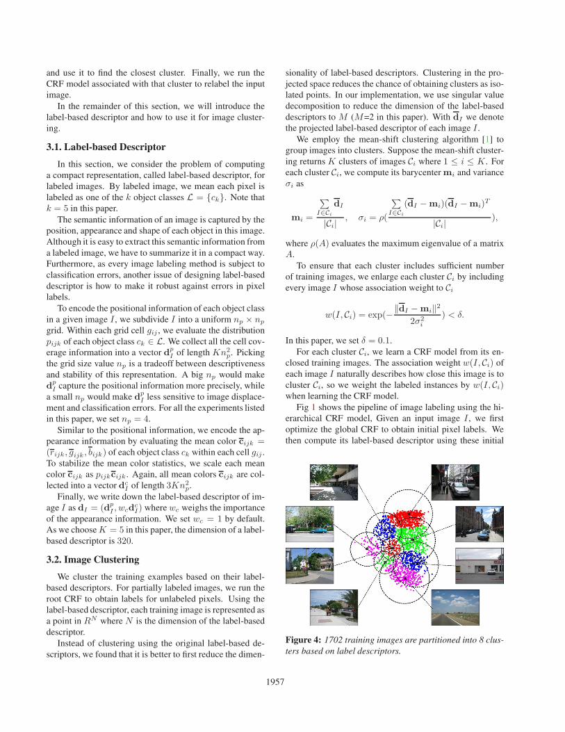
Fig 1 shows the pipeline of image labeling using the hi-erarchical CRF model, Given an input image I , we firstoptimize the global CRF to obtain initial pixel labels. Wethen compute its label-based descriptor using these initial

Figure 4: 1702 training images are partitioned into 8 clus-ters based on label descriptors.

1957

(a)

Per. Misc Sky Arch. Plant GroundMisc 15.9 72.3 0.0 5.2 7.4 15.1Sky 14.2 0.0 97.9 1.5 0.6 0.0

Arch. 30.9 2.3 4.2 81.4 6.9 5.2Plant 20.0 0.3 2.0 2.6 87.5 7.6

Ground 19.0 3.5 0.3 6.9 3.2 86.1

(b)

Unary CRFHe et al. 82.4 89.5

Shotton et al. 85.6 88.6Global 83.2 86.8

Hierarchical 86.1 90.7

(c)

Sky Vertical GroundSky 0.84/0.78 0.16/0.22 0.0/0.0

Vertical 0.06/0.09 0.91/0.89 0.03/0.02Ground 0.0/0.0 0.07/0.1 0.93/0.90

(d)

Per. Misc Sky Arch. Plant GroundMisc 3.1 71.8 0.1 9.2 4.4 14.5Sky 25.0 0.7 92.2 5.7 0.8 0.4

Arch. 48.3 4.3 3.2 83.1 4.2 5.2Plant 4.8 0.3 3.3 13.3 75.5 7.6

Ground 18.8 6.2 0.4 4.8 3.4 85.2

(e)

Per. Misc Sky Arch. Plant GroundMisc 4.9 65.6/76.5 0.9/0.5 14.9/10.2 3.5/3.5 15.1/9.3Sky 14.5 0.4/0.2 93.3/94.0 3.0/2.7 2.6/2.7 0.7/0.4

Arch. 41.5 4.8/3.5 2.4/2.3 81.1/84.0 7.2/5.8 4.5/4.4Plant 12.3 2.4/2.4 3.3/3.3 11.3/9.3 79.1/81.1 3.9/3.9

Ground 26.8 6.3/4.9 0.8/0.8 3.9/3.4 3.2/3.1 85.8/87.8

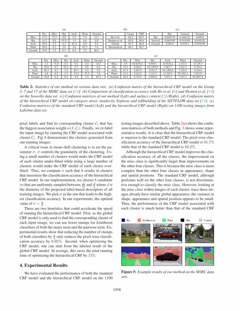
Table 2: Statistics of our method on various data sets. (a) Confusion matrix of the hierarchical CRF model on the Group3, 7 and 17 of the MSRC data set [14]. (b) Comparison of classification accuracy with He et al. [4] and Shotton et al. [14]on the Sowerby data set. (c) Confusion matrices of our method (Left) and surface context [5] (Right). (d) Confusion matrixof the hierarchical CRF model on category street, insidecity, highway and tallbuilding of the SIFTFLOW data set [15]. (e)Confusion matrices of the standard CRF model (Left) and the hierarchical CRF model (Right) on 1100 testing images fromLabelme data set.

pixel labels and find its corresponding cluster Ci that hasthe biggest association weight w(I, Ci). Finally, we re-labelthe input image by running the CRF model associated withcluster Ci. Fig 4 demonstrates the clusters generated fromour training images.

A critical issue in mean-shift clustering is to set the pa-rameter σ. σ controls the granularity of the clustering. Us-ing a small number of clusters would make the CRF modelof each cluster under-fitted while using a large number ofclusters would make the CRF model of each cluster over-fitted. Thus, we compute σ such that it results in clustersthat maximize the classification accuracy of the hierarchicalCRF model. In our implementation, we choose 8 candidateσs that are uniformly sampled between d

16 and d2 where d is

the diameter of the projected label-based descriptors of alltraining images. We pick σ as the one that leads to the high-est classification accuracy. In our experiments, the optimalvalue of σ = d

8 .There are two heuristics that could accelerate the speed

of running the hierarchical CRF model. First, as the globalCRF model is only used to find the corresponding cluster ofeach input image, we can use fewer stumps for Jointboostclassifiers of both the unary term and the pairwise term. Ex-perimental results show that reducing the number of stumpsof both classifiers by 3

4 only reduces the pixel-wise classifi-cation accuracy by 0.05%. Second, when optimizing theCRF model, one can start from the labeled result of theglobal CRF model. In average, this saves the total runningtime of optimizing the hierarchical CRF by 15%.

4. Experimental Results

We have evaluated the performance of both the standardCRF model and the hierarchical CRF model on the 1100

testing images described above. Table 2(e) shows the confu-sion matrices of both methods and Fig. 3 shows some repre-sentative results. It is clear that the hierarchical CRF modelis superior to the standard CRF model. The pixel-wise clas-sification accuracy of the hierarchical CRF model is 85.7%while that of the standard CRF model is 83.2%.

Although the hierarchical CRF model improves the clas-sification accuracy of all the classes, the improvement onthe misc class is significantly larger than improvements onthe other four classes. This is because the misc class is morecomplex than the other four classes in appearance, shapeand spatial positions. The standard CRF model, althoughperforms well on the other four classes, is not discrimina-tive enough to classify the misc class. However, looking atthe misc class within images of each cluster, since these im-ages already have similar global appearance, the variance inshape, appearance and spatial position appears to be small.Thus, the performance of the CRF model associated witheach cluster is much better than that of the standard CRF

Figure 5: Example results of our method on the MSRC datasets.

1958

model.Evaluation. We have compared our results with those ofHe et al [4] and those of Shotton et al.[14] on the Sowerbydata set used in [4]. As shown in Table. 2(b), the standardCRF model is slightly worse than their methods. This is be-cause the standard CRF model is trained from a wide rangeof images while the images in the Sowerby data set has re-stricted global appearance. However, the hierarchical CRFmodel, which learns a CRF model from the most similarcluster of images, turns out to be better than their methods.

We have also tested our method on the MSRC data set.In this experiment, we only tested three groups of imageswhich are related to images of street scenes (See Fig. 5 forexample results). Table 2(a) shows the confusion matrix ofthe hierarchical CRF model. On these three groups of im-ages, the pixel-wise classification accuracy of our methodis 84.5%, which is very competitive to the performance ofShotton et al. [14].

Moreover, we have compared our method with the sur-face context method [5] which segments an image into threeclasses: sky, vertical and ground. To make this comparison,we combine the plant class and the arch class as the verticalclass. In addition, we include the misc class into the groundclass. On the benchmark data set provides in [5], we im-proved the pixel-wise classification accuracy from [5] by3.7% (See Table 2(c) for details).

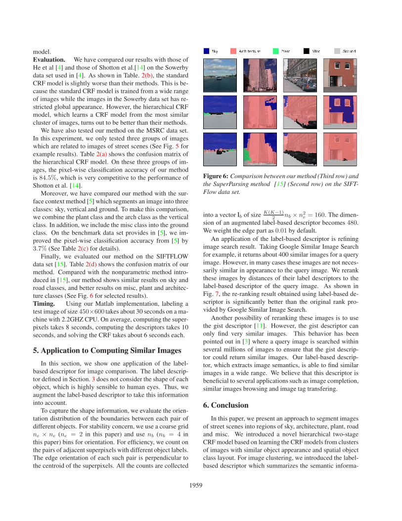
Finally, we evaluated our method on the SIFTFLOWdata set [15]. Table 2(d) shows the confusion matrix of ourmethod. Compared with the nonparametric method intro-duced in [15], our method shows similar results on sky androad classes, and better results on misc, plant and architec-ture classes (See Fig. 6 for selected results).Timing. Using our Matlab implementation, labeling atest image of size 450×600 takes about 30 seconds on a ma-chine with 2.2GHZ CPU. On average, computing the super-pixels takes 8 seconds, computing the descriptors takes 10seconds, and solving the CRF takes about 6 seconds each.

5. Application to Computing Similar Images

In this section, we show one application of the label-based descriptor for image comparison. The label descrip-tor defined in Section. 3 does not consider the shape of eachobject, which is highly sensible to human eyes. Thus, weaugment the label-based descriptor to take this informationinto account.

To capture the shape information, we evaluate the orien-tation distribution of the boundaries between each pair ofdifferent objects. For stability concern, we use a coarse gridne × ne (ne = 2 in this paper) and use nb (nb = 4 inthis paper) bins for orientation. For efficiency, we count onthe pairs of adjacent superpixels with different object labels.The edge orientation of each such pair is perpendicular tothe centroid of the superpixels. All the counts are collected

Figure 6: Comparison between our method (Third row) andthe SuperParsing method [15] (Second row) on the SIFT-Flow data set.

into a vector lb of size K(K−1)2 nb × n2

e = 160. The dimen-sion of an augmented label-based descriptor becomes 480.We weight the edge part as 0.01 by default.

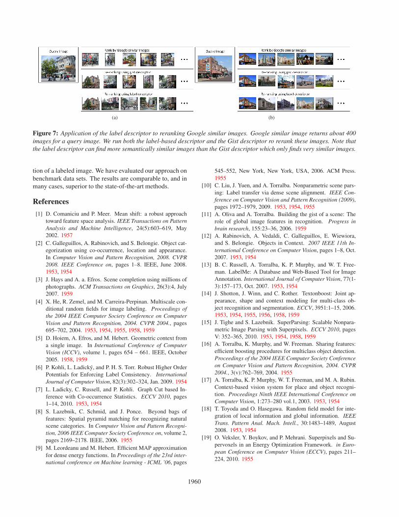
An application of the label-based descriptor is refiningimage search result. Taking Google Similar Image Searchfor example, it returns about 400 similar images for a queryimage. However, in many cases these images are not neces-sarily similar in appearance to the query image. We rerankthese images by distances of their label descriptors to thelabel-based descriptor of the query image. As shown inFig. 7, the re-ranking result obtained using label-based de-scriptor is significantly better than the original rank pro-vided by Google Similar Image Search.

Another possibility of reranking these images is to usethe gist descriptor [11]. However, the gist descriptor canonly find very similar images. This behavior has beenpointed out in [3] where a query image is searched withinseveral millions of images to ensure that the gist descrip-tor could return similar images. Our label-based descrip-tor, which extracts image semantics, is able to find similarimages in a wide range. We believe that this descriptor isbeneficial to several applications such as image completion,similar images browsing and image tag transfering.

6. Conclusion

In this paper, we present an approach to segment imagesof street scenes into regions of sky, architecture, plant, roadand misc. We introduced a novel hierarchical two-stageCRF model based on learning the CRF models from clustersof images with similar object appearance and spatial objectclass layout. For image clustering, we introduced the label-based descriptor which summarizes the semantic informa-

1959

(a) (b)

Figure 7: Application of the label descriptor to reranking Google similar images. Google similar image returns about 400images for a query image. We run both the label-based descriptor and the Gist descriptor ro rerank these images. Note thatthe label descriptor can find more semantically similar images than the Gist descriptor which only finds very similar images.

tion of a labeled image. We have evaluated our approach onbenchmark data sets. The results are comparable to, and inmany cases, superior to the state-of-the-art methods.

References

[1] D. Comaniciu and P. Meer. Mean shift: a robust approachtoward feature space analysis. IEEE Transactions on PatternAnalysis and Machine Intelligence, 24(5):603–619, May2002. 1957

[2] C. Galleguillos, A. Rabinovich, and S. Belongie. Object cat-egorization using co-occurrence, location and appearance.In Computer Vision and Pattern Recognition, 2008. CVPR2008. IEEE Conference on, pages 1–8. IEEE, June 2008.1953, 1954

[3] J. Hays and A. a. Efros. Scene completion using millions ofphotographs. ACM Transactions on Graphics, 26(3):4, July2007. 1959

[4] X. He, R. Zemel, and M. Carreira-Perpinan. Multiscale con-ditional random fields for image labeling. Proceedings ofthe 2004 IEEE Computer Society Conference on ComputerVision and Pattern Recognition, 2004. CVPR 2004., pages695–702, 2004. 1953, 1954, 1955, 1958, 1959

[5] D. Hoiem, A. Efros, and M. Hebert. Geometric context froma single image. In International Conference of ComputerVision (ICCV), volume 1, pages 654 – 661. IEEE, October2005. 1958, 1959

[6] P. Kohli, L. Ladicky, and P. H. S. Torr. Robust Higher OrderPotentials for Enforcing Label Consistency. InternationalJournal of Computer Vision, 82(3):302–324, Jan. 2009. 1954

[7] L. Ladicky, C. Russell, and P. Kohli. Graph Cut based In-ference with Co-occurrence Statistics. ECCV 2010, pages1–14, 2010. 1953, 1954

[8] S. Lazebnik, C. Schmid, and J. Ponce. Beyond bags offeatures: Spatial pyramid matching for recognizing naturalscene categories. In Computer Vision and Pattern Recogni-tion, 2006 IEEE Computer Society Conference on, volume 2,pages 2169–2178. IEEE, 2006. 1955

[9] M. Leordeanu and M. Hebert. Efficient MAP approximationfor dense energy functions. In Proceedings of the 23rd inter-national conference on Machine learning - ICML ’06, pages

545–552, New York, New York, USA, 2006. ACM Press.1955

[10] C. Liu, J. Yuen, and A. Torralba. Nonparametric scene pars-ing: Label transfer via dense scene alignment. IEEE Con-ference on Computer Vision and Pattern Recognition (2009),pages 1972–1979, 2009. 1953, 1954, 1955

[11] A. Oliva and A. Torralba. Building the gist of a scene: Therole of global image features in recognition. Progress inbrain research, 155:23–36, 2006. 1959

[12] A. Rabinovich, A. Vedaldi, C. Galleguillos, E. Wiewiora,and S. Belongie. Objects in Context. 2007 IEEE 11th In-ternational Conference on Computer Vision, pages 1–8, Oct.2007. 1953, 1954

[13] B. C. Russell, A. Torralba, K. P. Murphy, and W. T. Free-man. LabelMe: A Database and Web-Based Tool for ImageAnnotation. International Journal of Computer Vision, 77(1-3):157–173, Oct. 2007. 1953, 1954

[14] J. Shotton, J. Winn, and C. Rother. Textonboost: Joint ap-pearance, shape and context modeling for multi-class ob-ject recognition and segmentation. ECCV, 3951:1–15, 2006.1953, 1954, 1955, 1956, 1958, 1959

[15] J. Tighe and S. Lazebnik. SuperParsing: Scalable Nonpara-metric Image Parsing with Superpixels. ECCV 2010, pagesV: 352–365, 2010. 1953, 1954, 1958, 1959

[16] A. Torralba, K. Murphy, and W. Freeman. Sharing features:efficient boosting procedures for multiclass object detection.Proceedings of the 2004 IEEE Computer Society Conferenceon Computer Vision and Pattern Recognition, 2004. CVPR2004., 3(v):762–769, 2004. 1955

[17] A. Torralba, K. P. Murphy, W. T. Freeman, and M. A. Rubin.Context-based vision system for place and object recogni-tion. Proceedings Ninth IEEE International Conference onComputer Vision, 1:273–280 vol.1, 2003. 1953, 1954

[18] T. Toyoda and O. Hasegawa. Random field model for inte-gration of local information and global information. IEEETrans. Pattern Anal. Mach. Intell., 30:1483–1489, August2008. 1953, 1954

[19] O. Veksler, Y. Boykov, and P. Mehrani. Superpixels and Su-pervoxels in an Energy Optimization Framework. in Euro-pean Conference on Computer Vision (ECCV), pages 211–224, 2010. 1955

1960