A Heuristic for the Vehicle Routing Problem with Time Windows

Journal of Heuristics, 7: 107–129 (2001)c© 2001 Kluwer Academic Publishers

A Heuristic for the Vehicle Routing Problemwith Time Windows

ROBERTO CORDONEDipartimento di Elettronica e Informazione, Politecnico di Milano, Piazza Leonardo da Vinci, 32-20133,Milano, Italyemail: [email protected]

ROBERTO WOLFLER CALVOInstitute for Systems Informatics & Safety, Joint Research Centre (JRC) European Commission, via E. Fermi,1-21020 Ispra, Italy; Dipartimento di Elettronica e Informazione, Politecnico di Milano, Piazza Leonardo daVinci, 32-20133, Milano, Italyemail: [email protected]

Abstract

In this paper we propose a heuristic algorithm to solve the Vehicle Routing Problem with Time Windows. Itsframework is a smart combination of three simple procedures: the classicalk-optexchanges improve the solution,anad hocprocedure reduces the number of vehicles and a second objective function drives the search out of localoptima. No parameter tuning is required and no random choice is made: these are the distinguishing features withrespect to the recent literature. The algorithm has been tested on benchmark problems which prove it to be moreeffective than comparable algorithms.

Key Words: routing, scheduling, heuristics, local search, vehicle routing with time windows

1. Introduction

Vehicle routing problems arise whenever a set of vehicles is available to serve a set oftransportation requests. Each request specifies one or more locations that have to be visitedby the same vehicle and various side constraints that restrict the way to visit them. Themost common, both in practice and in the literature, refer to capacity and time. Capacityconstraints arise when customer locations require the vehicles to pick up or deliver loadsand the amount each vehicle can carry at the one time is limited. Time constraints usuallymodel the following situation: the service at each location can take place only during agiven interval, calledtime window.

In particular, this paper deals with the Vehicle Routing Problem with Time Windows(VRPTW). This problem consists of finding a set of routes that visit each request onceand only once at minimum cost. Each route, starting and ending at a specific location,calleddepot, has to satisfy both capacity and time window constraints. We deal with hardtime windows: given an interval[ei , l i ], the vehicle servicing nodei is bound to arrivebeforel i ; it may arrive beforeei , but then the service cannot start until the time window

108 CORDONE AND WOLFLER CALVO

begins. Once the service has begun, a given timesi must elapse before the vehicle mayleave.

At least four possible minimising objective functions have been considered in the liter-ature: the number of vehicles, the total travel time, the sum of completion times and thesum of all route durations. The duration of each route is measured as the difference be-tween its completion time and the latest feasible departure from the depot (Kindervater andSavelsbergh, 1997). In this paper, we adopt a two-level objective function: all customersmust be serviced with the minimum number of vehicles and, for the same number of routes,with the minimum total travel time.

The proposed algorithm, AKRed (Alternate K-exchange Reduction), is a two-phaseapproximation algorithm. It builds a set of initial solutions, improves them through a localsearch procedure and returns the best solution found. This is the simplest way to escapelocal optima, known asrestart. AKRed’s local search procedure combinesk-exchanges(between routes and inside a single route) and anad hocprocedure to reduce the numberof vehicles, calledReduction. Both take advantage of using a global best strategy and arenested in such a way that their interaction is as effective as possible. In fact, the interplaybetween them is one of AKRed’s most important features.

To move out of local optima, the algorithm applies the same local search procedure with aslightly different objective function, whose main component is still the number of vehicles,whereas the secondary component is the route duration, instead of the travel time. Once alocal optimum is attained, the initial objective function is restored and the search starts again.In a sense, this is still a descent method, since the current objective never worsens. Thisapproach, which is applied for the first time to a routing and scheduling problem, requires noadditional data structure and no random step, unlike Tabu Search, Genetic Algorithms andSimulated Annealing. Those strategies, although extremely effective, need a more or lesscomplex tuning phase and often a long computational time to obtain good results. AKRedhas no parameter to be fixed, proves reasonably fast and its results compare favourably withpreviously reported ones. The comparison has been made solving the 56 problems proposedby Solomon and four real world problems.

In the next section we present a classical formulation for the VRPTW, followed by abrief overview of the literature. The algorithm is described in section three. In section fourwe describe some implementation features to improve efficiency. Computational results onbenchmark problems and conclusions close the paper.

2. The vehicle routing problem with time windows

Let G = (N, A) be a directed graph, whereN = {0, 1, . . . ,n} is the node set andA = {(i, j ) : i, j ∈ N, i 6= j } is the arc set. Node 0 represents the depot andN ′ = {1, . . . ,n}denotes the set of nodes to be visited. Each arc(i, j ) is associated to a travel costcij ≥ 0and a travel timetij ≥ 0. Each nodei has a service requestqi , a service timesi and atime window[ei , l i ]. All vehicles have the same capacityQ and the same costh ≥ 0. In thefollowing, we are assuming thatcij = tij , ∀(i, j ) ∈ A and thath is high enough to guaranteethat minimising the number of vehicles is the main objective. Without loss of generality,

A HEURISTIC FOR THE VEHICLE ROUTING PROBLEM 109

we may shrink the time windows by settingei = max(e0+ t0i , ei )andl i = min(l0− ti 0, l i ).In fact, this removes portions which cannot be feasibly used (Desrochers et al., 1992).

Let us setxi j = 1 if arc (i, j ) is used,xi j = 0 otherwise;pi represents the beginningof the service at nodei ; yi is the load of the vehicle leaving nodei . The mathematicalformulation of the VRPTW may then be defined as follows:

min∑j∈N ′

hx0 j +∑(i, j )∈A

cij xij (1)

subject to: ∑j∈N

xij = 1 ∀i ∈ N ′ (2)∑i∈N

xij = 1 ∀ j ∈ N ′ (3)

if xij = 1⇒ pi + si + tij ≤ pj ∀(i, j ) ∈ A (4)

ei ≤ pi ≤ l i ∀i ∈ N ′ (5)

if xij = 1⇒ yi + qj ≤ yj ∀(i, j ) ∈ A (6)

qi ≤ yi ≤ Q ∀i ∈ N ′ (7)

xi j ∈ {0, 1} ∀(i, j ) ∈ A (8)

The constraints (2) and (3) ensure that each customer be assigned exactly to a single route.The Eqs. (4) and (5) represent time window constraints, while Eqs. (6) and (7) representcapacity constraints.

Although the VRPTW is NP-hard (Savelsbergh, 1985), many exact algorithms havebeen proposed in the literature: see, for instance, Fisher and Jaikumar (1981), Kolen et al.(1987), Desrochers et al. (1992), and, more recently, Fisher et al. (1997), Kohl and Madsen(1997), and Kohl et al. (1997). These algorithms can solve instances up to one hundrednodes, provided that the time windows are very tight. When larger instances or wider timewindows are tackled, heuristics are needed.

The approximation algorithms can be broadly classified into two types: constructive andimproving.

As for constructive heuristics, Solomon was the first who adapted to the VRPTW anumber of criteria used to solve the Vehicle Routing Problem (Solomon, 1987). Thesealgorithms are very fast, but usually the solution is not very good.

The earliest improving algorithms, developed by Russell (1977) and later by Baker andShaffer (1986), were local search procedures exploiting Lin and Kernighan’sk-optexchangeapproach (Lin and Kernighan, 1973). This family of exchanges is effective, but fork greaterthan two it suffers from a very large processing time. Savelsbergh (1985) proposed anefficient implementation for routing problems with time windows. Potvin and Rousseau(1993) described an effective algorithm based on a parallel insertion heuristic and on theOr-opt exchanges (a special case of 3-opt exchange which is less powerful, but faster(Or, 1976)). Kontoravdis and Bard (1995) combined a greedy randomized adaptive searchprocedure (GRASP) to build a feasible solution and a local search scheme to improve


upon it. Moreover, they pointed out some criteria to estimate a lower bound on the fleetsize. A hybrid algorithm was proposed by Russell (1995): the constructive procedure isperiodically stopped and the local search procedure is applied to improve the current partialsolution.

All of the latest algorithms in the literature are metaheuristic. Metaheuristics, such asSimulated AnnealingandTabu Search, can be viewed as improvement methods. These aresearch schemes in which consecutive neighbours of a solution are explored and, in orderto avoid local minima, the objective is allowed to worsen. Potvin and Bengio (1996) useda genetic approach. A combination of Genetic Algorithm, Simulated Annealing and TabuSearch was proposed by Thangiah et al. (1994). Potvin et al. (1996) implemented a pureTabu Search. Chiang and Russell (1996) described an algorithm which enhances Russell’salgorithm with a Simulated Annealing strategy. Rochat and Taillard (1995) suggested tofeedback a Tabu Search algorithm proposed in Rochat and Semet (1994) with a probabilisticintensification and diversification strategy. The same concept underlies an algorithm pro-posed by Taillard et al. (1997) to solve soft time window problems. This algorithm, whichhas also been tested on hard time windows, crosses unfeasible solutions and uses a furtherfamily of exchanges.

A good survey on the subject can be found in Desrosiers et al. (1995).

3. The algorithm

AKRed, as most approximation algorithms, begins by building an initial feasible solution.Little is worth saying about this phase, since it creates eight initial solutions using the

first set of criteria proposed by Solomon (1987). In short, the algorithm starts with no routesand no node serviced. A single route is opened and initialized with aseednodes∗, which iseither the farthest from the depot (s∗ = arg maxs t0s) or the one whose time window beginsfirst (s∗ = arg mins es). Then, all feasible insertions of each unserviced nodeu betweentwo adjacent nodesi and j of the current route are evaluated. This is done according toa suitable cost functionc1, which is either(tiu + tuj − tij ) or (pnew

j − poldj ), where pold

j(respectively,pnew

j ) is the time when service begins at nodej before (respectively, after)the insertion. The best insertion point for nodeu is thereforei ∗ (u) = arg mini c1 (u, i ). Adifferent cost functionc2 determines which node to choose:c2 is eitherc1 (u, i ∗ (u))− t0u orc1 (u, i ∗ (u))−2t0u. Its purpose is to maximise the benefit derived from servicing nodeu onthe current route rather than on a dedicated one. Thus, nodeu∗ = arg minu c2 (u, i ∗ (u)) ischosen and inserted after nodei ∗ (u∗). If there is no feasible insertion point, but still nodesto be serviced, another route is opened and initialized. It is assumed, in fact, that all requestscan be satisfied, at least, by a dedicated vehicle. The procedure stops when no request is left.

Starting from these initial solutions, better ones are obtained through a local searchalgorithm. Local search is based on the concept ofneighbourhood, which is the set of allsolutions achievable from the current one applying a given family of transformations. Theprocedure looks for an improved solution in this neighbourhood and if one exists, it replacesthe old one; otherwise, the procedure stops.

AKRed uses two nested local search procedures. The external one (K-exchange) ap-plies thek-optexchanges withk≤ 3, namely 2-exchanges and 3-exchanges between routes


(inter-route) and inside a single route (intra-route). It always chooses the best solution in thewhole neighbourhood (global beststrategy), but the neighbourhood itself is not completelyexplored every time, since a smart technique permits it to remain updated (see Section 3.4).The inner level (Reduction) is a proceduread hocto decrease the number of routes. It triesto remove each route by displacing all of its nodes into the other ones. Solutions with thesame number of vehicles, but a smaller travel time, are accepted, since they are profitableaccording to the objective function.

The local search phase stops when the solution cannot be improved any more, as itreaches a local optimum. Then a third, more external procedure (Alternate), generates anew starting point by running the local search with a subservient objective function: themain component is still the number of vehicles, but the secondary component is the routeduration. Most times, this is enough to drive the search away, since the solution is no longera local optimum. When a local optimum with respect to this second function is reached,AKRed goes back to the original objective and starts again. To avoid a cyclic behaviour, theprocedure stops when a “double” step leads back to the same solution or to a worse one.

A pseudocode of the algorithm follows. Given a solutions, vectorz(s) denotes the valueof the objective function: its first element is the number of vehicles, the second one the totaltravel time. Vectorw (s) denotes the value of the function used to generate new startingpoints: its first element is the number of vehicles, the second one the total route duration.Comparisons are carried out in a lexicographic fashion. Subscriptref refers to the bestsolution obtained during the current restart iteration, superscript∗ to the best obtained sofar.

Algorithm AKRedz∗ := ∞;For i := 1 to 8 do{Build a new initial solution using Solomon’si−th algorithm}s := SolomonInsertion(i ) ;zref := ∞;While z(s) < zref do

sref := s; zref := z(sref ); {Update the best solution of iterationi }{Improve solutions with respect tow by k-exchanges andReduction1}s := LocalSearch(s, w) ;{Improve solutions with respect toz by k-exchanges andReduction}s := LocalSearch(s, z) ;

EndWhile;If zref < z∗ then s∗ = sref ; z∗ = zref ; {Update the best solution}

EndFor;Return(s∗, z∗) ;End.

This is a pseudocode of the local search procedure: parameterOb defines the objectivefunction whose minimisation is currently pursued, eitherz orw. Subscriptcur refers to thebest solution found so far.


ProcedureLocalSearch(s,Ob)Obcur := ∞;While Ob(s) < Obcur do

Repeatscur := s; Obcur := Ob(s) ; {Update the best solution}s := Reduction(s,Ob) ;

Until Ob(s) < Obcur; {Apply Reductionas long as the solution improves}s := K-exchange(scur,Ob) ; {Apply a single step ofK-exchange}

EndWhile;Return scur;End.

3.1. K-exchange

A k-exchange consists of replacingk arcs of the current solution by another set ofk arcsin order to create a new one. Thek-neighbourhood is the set of solutions which can beobtained from the initial one by ak-exchange.

In multi-vehicle problems thek arcs can be chosen from a single route (intra-route) ormore (inter-route). Both exchanges are essential, since the intra-route ones improve thesequence of nodes serviced by a vehicle, whereas inter-route exchanges determine the as-signment of nodes to vehicles. Thek-neighbourhood containsO(nk) solutions, so that itscomplete exploration requiresO(nk) time, provided that the feasibility and profitability ofeach neighbour solution is checked in constant time. Not surprisingly, much better solu-tions may be found when the neighbourhood is enlarged by increasing the numberk ofarcs to be replaced. Unfortunately, the computational effort required to search the neigh-bourhood becomes much greater as well. Nevertheless, in AKRed we use 2-exchanges and3-exchanges and we adopt a global best strategy, always looking for the best solution in thewhole neighbourhood.

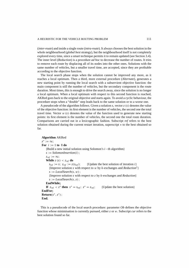
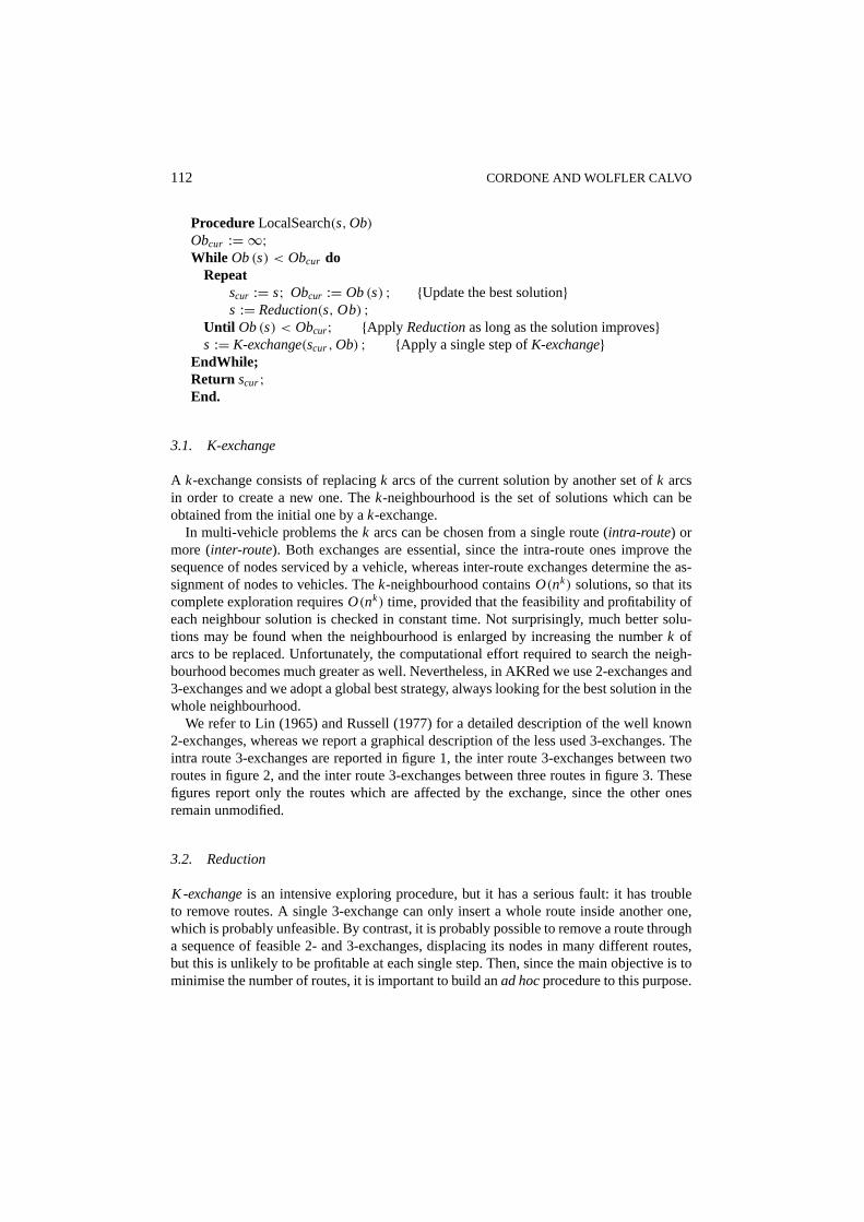
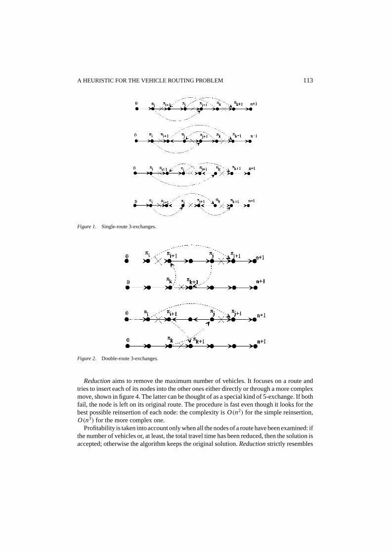
We refer to Lin (1965) and Russell (1977) for a detailed description of the well known2-exchanges, whereas we report a graphical description of the less used 3-exchanges. Theintra route 3-exchanges are reported in figure 1, the inter route 3-exchanges between tworoutes in figure 2, and the inter route 3-exchanges between three routes in figure 3. Thesefigures report only the routes which are affected by the exchange, since the other onesremain unmodified.

3.2. Reduction

K-exchangeis an intensive exploring procedure, but it has a serious fault: it has troubleto remove routes. A single 3-exchange can only insert a whole route inside another one,which is probably unfeasible. By contrast, it is probably possible to remove a route througha sequence of feasible 2- and 3-exchanges, displacing its nodes in many different routes,but this is unlikely to be profitable at each single step. Then, since the main objective is tominimise the number of routes, it is important to build anad hocprocedure to this purpose.


Figure 1. Single-route 3-exchanges.

Figure 2. Double-route 3-exchanges.

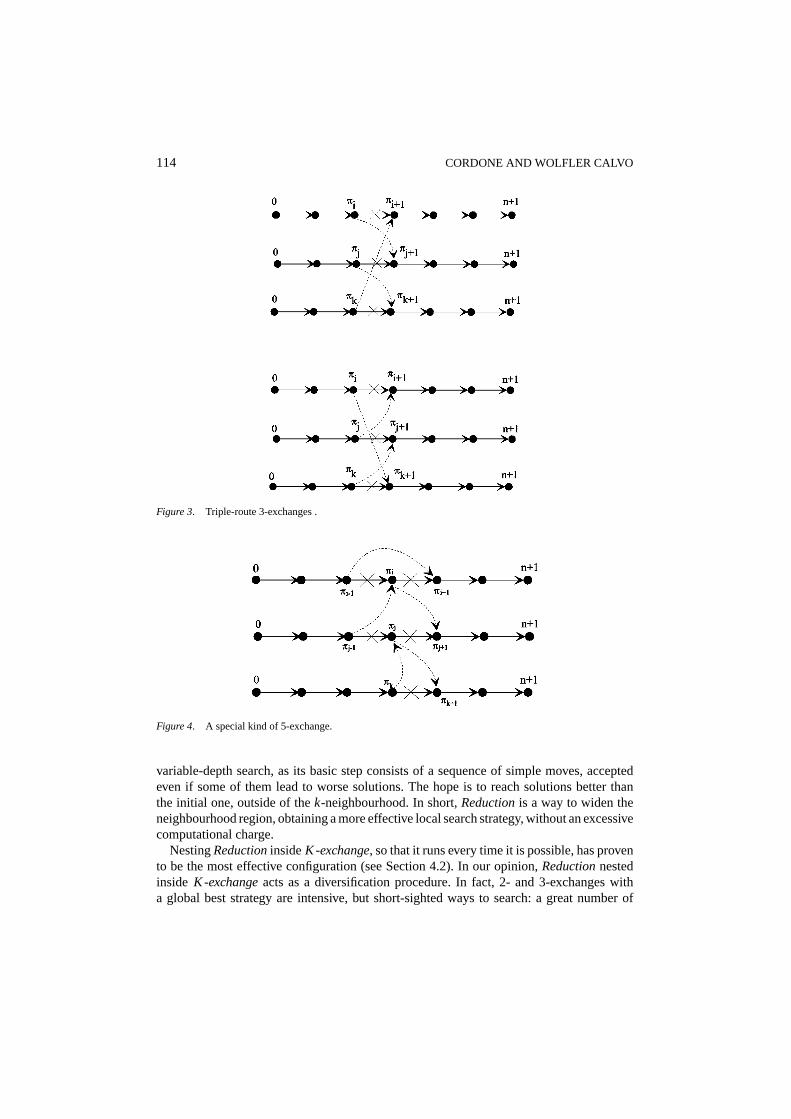
Reductionaims to remove the maximum number of vehicles. It focuses on a route andtries to insert each of its nodes into the other ones either directly or through a more complexmove, shown in figure 4. The latter can be thought of as a special kind of 5-exchange. If bothfail, the node is left on its original route. The procedure is fast even though it looks for thebest possible reinsertion of each node: the complexity isO(n2) for the simple reinsertion,O(n3) for the more complex one.

Profitability is taken into account only when all the nodes of a route have been examined: ifthe number of vehicles or, at least, the total travel time has been reduced, then the solution isaccepted; otherwise the algorithm keeps the original solution.Reductionstrictly resembles


Figure 3. Triple-route 3-exchanges .

Figure 4. A special kind of 5-exchange.

variable-depth search, as its basic step consists of a sequence of simple moves, acceptedeven if some of them lead to worse solutions. The hope is to reach solutions better thanthe initial one, outside of thek-neighbourhood. In short,Reductionis a way to widen theneighbourhood region, obtaining a more effective local search strategy, without an excessivecomputational charge.

NestingReductioninsideK-exchange, so that it runs every time it is possible, has provento be the most effective configuration (see Section 4.2). In our opinion,Reductionnestedinside K-exchangeacts as a diversification procedure. In fact, 2- and 3-exchanges witha global best strategy are intensive, but short-sighted ways to search: a great number of


neighbours are considered, but they are very “near” to the original solution (only 2 or 3 arcsdiffer). On the contrary,Reductionneighbours are few (one for each route) and tend to beas far as possible from the current solution. Evidence that diversification is a key featurein Reductionis given by the failure of a variant: this version evaluates all intermediatesolutions crossed, as nodes are removed one by one, and chooses the best, instead of the lastone. Though this neighbourhood is wider, the procedure proves less effective on average.

Several different versions have been tested to examine other features. Experience showsthat it is better to applyReductionfirst to shorter routes, but without focussing exclusivelyon them. So, we order the routes by non decreasing lengths and try to remove each of them;a route is taken again into account only when all the others have been considered.

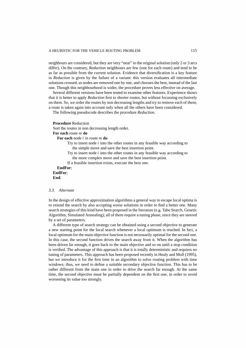
The following pseudocode describes the procedureReduction.

ProcedureReductionSort the routes in non decreasing length order.For eachroutem do

For eachnodei in routem doTry to insert nodei into the other routes in any feasible way according to

the simple move and save the best insertion point.Try to insert nodei into the other routes in any feasible way according to

the more complex move and save the best insertion point.If a feasible insertion exists, execute the best one.

EndFor;EndFor;End.

3.3. Alternate

In the design of effective approximation algorithms a general way to escape local optima isto extend the search by also accepting worse solutions in order to find a better one. Manysearch strategies of this kind have been proposed in the literature (e.g. Tabu Search, GeneticAlgorithm, Simulated Annealing); all of them require a tuning phase, since they are steeredby a set of parameters.

A different type of search strategy can be obtained using a second objective to generatea new starting point for the local search whenever a local optimum is reached. In fact, alocal optimum for the main objective function is not necessarily optimal for the second one.In this case, the second function drives the search away from it. When the algorithm hasbeen driven far enough, it goes back to the main objective and so on until a stop conditionis verified. The advantage of this approach is that it is totally deterministic and requires notuning of parameters. This approach has been proposed recently in Healy and Moll (1995),but we introduce it for the first time in an algorithm to solve routing problem with timewindows; thus, we need to define a suitable secondary objective function. This has to berather different from the main one in order to drive the search far enough. At the sametime, the second objective must be partially dependent on the first one, in order to avoidworsening its value too strongly.


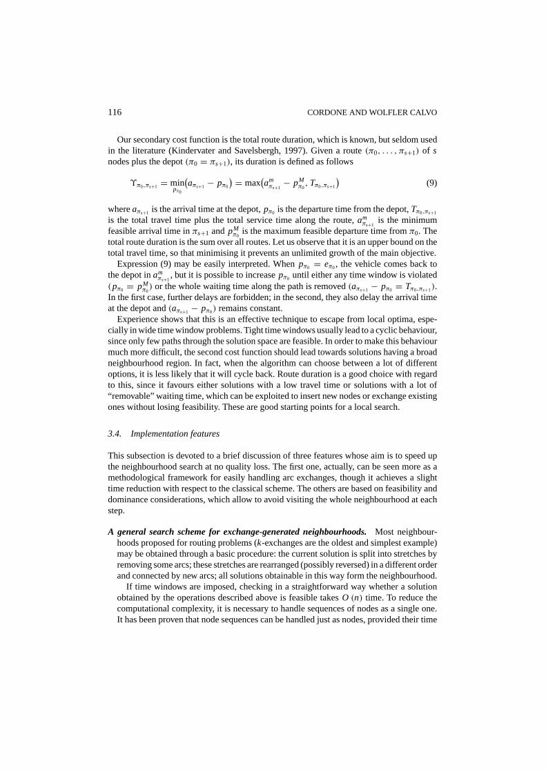
Our secondary cost function is the total route duration, which is known, but seldom usedin the literature (Kindervater and Savelsbergh, 1997). Given a route(π0, . . . , πs+1) of snodes plus the depot(π0 = πs+1), its duration is defined as follows

ϒπ0,πs+1 = minpπ0

(aπs+1 − pπ0

) = max(amπs+1− pM

π0, Tπ0,πs+1

)(9)

whereaπs+1 is the arrival time at the depot,pπ0 is the departure time from the depot,Tπ0,πs+1

is the total travel time plus the total service time along the route,amπs+1

is the minimumfeasible arrival time inπs+1 andpM

π0is the maximum feasible departure time fromπ0. The

total route duration is the sum over all routes. Let us observe that it is an upper bound on thetotal travel time, so that minimising it prevents an unlimited growth of the main objective.

Expression (9) may be easily interpreted. Whenpπ0 = eπ0, the vehicle comes back tothe depot inam

πs+1, but it is possible to increasepπ0 until either any time window is violated

(pπ0 = pMπ0) or the whole waiting time along the path is removed(aπs+1 − pπ0 = Tπ0,πs+1).

In the first case, further delays are forbidden; in the second, they also delay the arrival timeat the depot and(aπs+1 − pπ0) remains constant.

Experience shows that this is an effective technique to escape from local optima, espe-cially in wide time window problems. Tight time windows usually lead to a cyclic behaviour,since only few paths through the solution space are feasible. In order to make this behaviourmuch more difficult, the second cost function should lead towards solutions having a broadneighbourhood region. In fact, when the algorithm can choose between a lot of differentoptions, it is less likely that it will cycle back. Route duration is a good choice with regardto this, since it favours either solutions with a low travel time or solutions with a lot of“removable” waiting time, which can be exploited to insert new nodes or exchange existingones without losing feasibility. These are good starting points for a local search.

3.4. Implementation features

This subsection is devoted to a brief discussion of three features whose aim is to speed upthe neighbourhood search at no quality loss. The first one, actually, can be seen more as amethodological framework for easily handling arc exchanges, though it achieves a slighttime reduction with respect to the classical scheme. The others are based on feasibility anddominance considerations, which allow to avoid visiting the whole neighbourhood at eachstep.

A general search scheme for exchange-generated neighbourhoods.Most neighbour-hoods proposed for routing problems (k-exchanges are the oldest and simplest example)may be obtained through a basic procedure: the current solution is split into stretches byremoving some arcs; these stretches are rearranged (possibly reversed) in a different orderand connected by new arcs; all solutions obtainable in this way form the neighbourhood.

If time windows are imposed, checking in a straightforward way whether a solutionobtained by the operations described above is feasible takesO (n) time. To reduce thecomputational complexity, it is necessary to handle sequences of nodes as a single one.It has been proven that node sequences can be handled just as nodes, provided their time


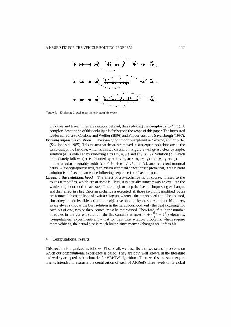
Figure 5. Exploring 2-exchanges in lexicographic order.

windows and travel times are suitably defined, thus reducing the complexity toO (1). Acomplete description of this technique is far beyond the scope of this paper. The interestedreader can refer to Cordone and Wolfler (1996) and Kindervater and Savelsbergh (1997).

Pruning unfeasible solutions. Thek-neighbourhood is explored in “lexicographic” order(Savelsbergh, 1985). This means that the arcs removed in subsequent solutions are all thesame except the last one, which is shifted on and on. Figure 5 will give a clear example:solution (a) is obtained by removing arcs(πi , πi+1) and(π j , π j+1). Solution (b), whichimmediately follows (a), is obtained by removing arcs(πi , πi+1) and(π j+1, π j+2).

If triangular inequality holds (thl ≤ thk + tkl , ∀h, k, l ∈ N), arcs represent minimalpaths. A lexicographic search, then, yields sufficient conditions to prove that, if the currentsolution is unfeasible, an entire following sequence is unfeasible, too.

Updating the neighbourhood. The effect of ak-exchange is, of course, limited to theroutes it modifies, which are at mostk. Thus, it is actually unnecessary to evaluate thewhole neighbourhood at each step. It is enough to keep the feasible improving exchangesand their effect in a list. Once an exchange is executed, all those involving modified routesare removed from the list and evaluated again, whereas the others need not to be updated,since they remain feasible and alter the objective function by the same amount. Moreover,as we always choose the best solution in the neighbourhood, only the best exchange foreach set of one, two or three routes, must be maintained. Therefore, ifm is the numberof routes in the current solution, the list contains at mostm + (m

2) + (m

3) elements.

Computational experiments show that for tight time window problems, which requiremore vehicles, the actual size is much lower, since many exchanges are unfeasible.

4. Computational results

This section is organized as follows. First of all, we describe the two sets of problems onwhich our computational experience is based. They are both well known in the literatureand widely accepted as benchmarks for VRPTW algorithms. Then, we discuss some exper-iments intended to evaluate the contribution of each of AKRed’s three levels to its global


performance. In the end, a comparison with the most effective algorithms proposed in theliterature is carried on.

We must point out that in this section we confront with results obtained by the other authorsin single experiments, with a specified number of runs and given parameters. Best knownresults are reported as a reference, but it would be meaningless to compare a single algorithmto a whole experimental campaign. As some authors report instance by instance results andsome others report average results on each problem set, we give both comparisons.

4.1. Benchmark problems

We have applied AKRed to the six VRPTW data sets R1, R2, C1, C2, RC1 and RC2generated by Solomon (1987), which are commonly accepted as the main benchmark forVRPTW algorithms. They are 56 random problems made up of 100 nodes. Vehicle capacity,customer time windows, service times and distribution in space and time vary so as to coverall configurations as thoroughly as possible. Thus, customers may be uniformly distributed(problem sets R1 and R2), clustered (problem sets C1 and C2), or a mix of the two patterns(problem sets RC1 and RC2). Problem sets R1, C1 and RC1 have a narrow schedulinghorizon, tight time windows and a low vehicle capacity. Conversely, problem sets R2, C2and RC2 have a large scheduling horizon, wide time windows and a high vehicle capacity.

We have also applied AKRed to four real world problems. The first two, D249 and E249,consist of 249 customers (Baker and Shaffer, 1986). They only differ in the vehicle capacity,which is fixed to 50 and 100 respectively. The second two problems, namely D417 and E417,consist of 419 customers and differ in that E417 has a higher number of tight time windows(Russell, 1995).

In both sets travel times correspond to euclidean distances. This has a disagreeablesecondary effect, due to rounding and truncating. Each author uses his own approximationdegree, so that they actually solve different, though much similar, problems, and obtaindifferent solutions. In our experience, at least three decimal digits seem necessary in orderto avoid this effect. In all of these problems, the main objective function is the number ofvehicles; the total travel time is the secondary function.

4.2. Experiments on Solomon’s problems

As we have pointed out, AKRed’s peculiarity is a three-level structure: a traditionalK-exchangeprocedure is enhanced by aReductionprocedure nested inside it and by an externalAlternatescheme. In this subsection we intend to quantify experimentally the contributioneach of these levels gives to the global performance.

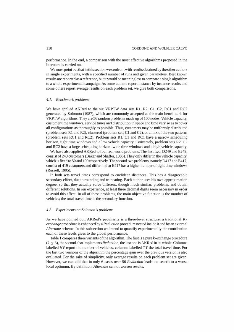
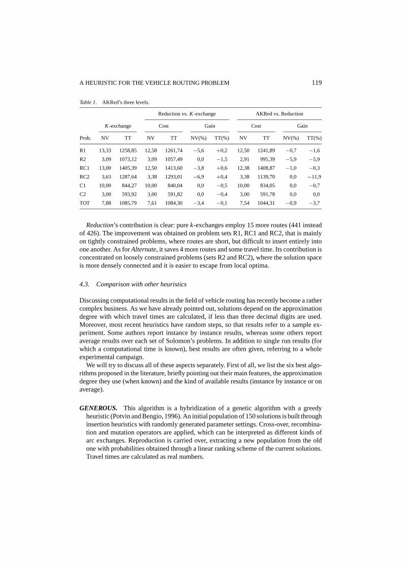
Table 1 compares three variants of the algorithm. The first is a purek-exchange procedure(k ≤ 3), the second also implementsReduction, the last one is AKRed in its whole. ColumnslabelledNV report the number of vehicles, columns labelledTT the total travel time. Forthe last two versions of the algorithm the percentage gain over the previous version is alsoevaluated. For the sake of simplicity, only average results on each problem set are given.However, we can add that in only 6 cases over 56Reductionleads the search to a worselocal optimum. By definition,Alternatecannot worsen results.


Table 1. AKRed’s three levels.

Reduction vs.K -exchange AKRed vs. Reduction

K -exchange Cost Gain Cost Gain

Prob. NV TT NV TT NV(%) TT(%) NV TT NV(%) TT(%)

R1 13,33 1258,85 12,58 1261,74 −5,6 +0,2 12,50 1241,89 −0,7 −1,6

R2 3,09 1073,12 3,09 1057,49 0,0 −1,5 2,91 995,39 −5,9 −5,9

RC1 13,00 1405,39 12,50 1413,60 −3,8 +0,6 12,38 1408,87 −1,0 −0,3

RC2 3,63 1287,64 3,38 1293,01 −6,9 +0,4 3,38 1139,70 0,0 −11,9

C1 10,00 844,27 10,00 840,04 0,0 −0,5 10,00 834,05 0,0 −0,7

C2 3,00 593,92 3,00 591,82 0,0 −0,4 3,00 591,78 0,0 0,0

TOT 7,88 1085,79 7,61 1084,30 −3,4 −0,1 7,54 1044,31 −0,9 −3,7

Reduction’s contribution is clear: purek-exchanges employ 15 more routes (441 insteadof 426). The improvement was obtained on problem sets R1, RC1 and RC2, that is mainlyon tightly constrained problems, where routes are short, but difficult to insert entirely intoone another. As forAlternate, it saves 4 more routes and some travel time. Its contribution isconcentrated on loosely constrained problems (sets R2 and RC2), where the solution spaceis more densely connected and it is easier to escape from local optima.

4.3. Comparison with other heuristics

Discussing computational results in the field of vehicle routing has recently become a rathercomplex business. As we have already pointed out, solutions depend on the approximationdegree with which travel times are calculated, if less than three decimal digits are used.Moreover, most recent heuristics have random steps, so that results refer to a sample ex-periment. Some authors report instance by instance results, whereas some others reportaverage results over each set of Solomon’s problems. In addition to single run results (forwhich a computational time is known), best results are often given, referring to a wholeexperimental campaign.

We will try to discuss all of these aspects separately. First of all, we list the six best algo-rithms proposed in the literature, briefly pointing out their main features, the approximationdegree they use (when known) and the kind of available results (instance by instance or onaverage).

GENEROUS. This algorithm is a hybridization of a genetic algorithm with a greedyheuristic (Potvin and Bengio, 1996). An initial population of 150 solutions is built throughinsertion heuristics with randomly generated parameter settings. Cross-over, recombina-tion and mutation operators are applied, which can be interpreted as different kinds ofarc exchanges. Reproduction is carried over, extracting a new population from the oldone with probabilities obtained through a linear ranking scheme of the current solutions.Travel times are calculated as real numbers.


The results refer to a single experiment made up of 50 generations. The algorithm runson a SPARC 10 workstation.

CR. The algorithm proposed by Chiang and Russell (1996) is based on Simulated Anneal-ing. Initial solutions are built through a parallel insertion heuristic, which is periodicallyinterrupted so that the current solution can be improved by an exchange procedure.The results refer to a collection of three algorithms, arising from two different defini-tions of neighbourhood: the second one, in fact, is explored both by a pure SimulatedAnnealing scheme and by a hybrid Tabu Search. Travel times are calculated as realnumbers.

The algorithm was implemented in Fortran on a 486 DX2/66 machine.GenSAT. The GenSAT system proposed by Thangiah et al. (1994) is a collection of eight

algorithms, resulting from three different choices. The first one refers to the initial solutionconstruction, which can be done through a simple insertion heuristic or a genetic sectoringheuristic. The second one determines the new solution at each step: it can be the firstimproving or the best in the whole neighbourhood. The last choice is between a pureTabu Search or a hybrid Tabu Search-Simulated Annealing scheme.

All the algorithms have been written in C and tested on a NeXT 68040 (25 MHz)machine. Results and computational times refer to the whole system.

RS. This is a pure Tabu Search heuristic (Rochat and Semet, 1994), for which two exper-iments are reported in Rochat and Taillard (1995). In the former, minimum, average andmaximum results over five different runs are evaluated: a single run consists, respectively,of 50 000, 150 000 and 300 000 iterations. In the latter, for which instance by instanceresults are given, each of the five runs performed 400 000 iterations.

Computational times refer to a Silicon Graphics Indigo (100 MHz).RT. We mean by this the intensification and diversification strategy described by Rochat

and Taillard (1995). First, a pool of routes is built by running 20 times the RS heuristicfor 2 000 iterations. Then, the search enters a feedback loop, which consists of buildinga new solution with routes taken from the pool, improving it with 2 000 iterations of RSand inserting the improved routes in the pool. Average results are reported for a single runmade up of 50 000, 150 000 and 300 000 iterations (respectively 5, 55 and 130 feedbackloops, plus the initial 20 loops).

Computational times refer to a Silicon Graphics Indigo (100 MHz).TBGGP. This algorithm by Taillard et al. (1997) applies the same intensification and

diversification strategy as RT: a Tabu Search procedure is interrupted every 330 iterationsand initialized with a new solution built from a pool of routes, made up of the 30 bestsolutions reached so far. However, the basic algorithm crosses unfeasible solutions, too,and a particular kind of 4-exchange, named CROSS-exchange, is implemented. Traveltimes are rounded at the third decimal place. Minimum, average and maximum resultsover five independent runs are reported. Each run is made up of, respectively, 0, 30 and80 restarts from the route pool, plus 20 initial loops to build it.

The algorithm has been tested on a SPARC 10 workstation (50 MHz).AKRed. AKRed has been written in Fortran 77 and tested on a Pentium 166 MHz. Travel

times are obtained by rounding distances to four decimal places, in order to avoid anydependence of the results on the approximation degree. We point out that this algorithm


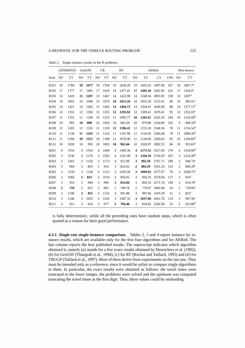
Table 2. Single-instance results on the R problems.

GENEROUS GenSAT CR RS AKRed Best known

Prob. NV TT NV TT NV TT NV TT NV TT CT CPU NV TT

R101 19 1784 18 1677 19 1704 19 1656.20 19 1652.63 3497.06 167 18 1607.7a

R102 17 1777 17 1493 17 1610 18 1477.4117 1491.18 3202.95 223 17 1434.0a

R103 14 1433 13 1207 13 1467 14 1422.90 14 1248.04 2805.95 158 13 1207b

R104 10 1065 10 1048 10 107910 1013.26 10 1052.59 2233.41 99 10 982.01c

R105 14 1421 14 1442 15 146514 1404.75 14 1418.41 2646.09 98 14 1377.11d

R106 12 1353 12 1350 12 135312 1293.92 12 1309.41 2479.41 95 12 1252.03c

R107 11 1191 11 1140 10 1215 11 1085.7710 1201.67 2241.55 104 10 1126.69d

R108 10 993 10 898 10 1003 10 965.28 10 979.86 2164.89 103 9 968.59d

R109 12 1205 12 1226 12 123912 1186.41 12 1235.30 2348.36 78 11 1214.54d

R110 11 1136 11 1105 11 1152 11 1107.90 11 1156.05 2266.68 78 11 1080.36d

R111 11 1184 10 1151 10 1188 11 1070.90 11 1128.66 2360.62 95 10 1104.83d

R112 10 1020 10 992 10 100310 965.66 10 1028.87 2082.52 84 10 953.63c

R201 4 1554 4 1354 4 1494 4 1485.364 1273.52 3527.69 170 4 1254.80d

R202 3 1530 4 1176 3 1562 4 1101.493 1264.56 2743.29 203 3 1214.28d

R203 3 1201 3 1126 3 1173 4 912.98 3 993.50 2767.71 188 3 948.74c

R204 3 904 3 803 2 914 3 824.62 2 884.29 1931.33 153 2 869.29c

R205 3 1159 3 1128 3 1212 3 1205.583 1099.02 2577.67 76 3 1038.72d

R206 3 1066 3 833 3 1074 3 956.05 3 936.76 2579.04 117 3 833c

R207 3 954 3 904 3 999 3 814.84 3 864.32 2571.74 149 3 814.78c

R208 2 759 2 823 2 805 3 708.78 2 779.07 1869.68 54 2 738.60c

R209 3 1108 3 855 3 1132 4 901.88 3 997.66 2419.39 51 3 855c

R210 3 1146 3 1052 3 1245 3 1087.323 1037.80 2601.76 119 3 967.50c

R211 3 913 3 816 3 977 3 794.46 3 818.82 2245.58 52 2 923.80d

is fully deterministic, while all the preceding ones have random steps, which is oftenquoted as a reason for their good performance.

4.3.1. Single-run single-instance comparison.Tables 2, 3 and 4 report instance by in-stance results, which are available only for the first four algorithms and for AKRed. Thelast column reports the best published results. The superscript indicates which algorithmobtained it, namely (a) stands for a few exact results obtained by Desrochers et al. (1992),(b) for GenSAT (Thangiah et al., 1994), (c) for RT (Rochat and Taillard, 1995) and (d) forTBGGP (Taillard et al., 1997). Most of them derive from experiments on the last one. Theymust be intended only as a reference, since it would be unfair to compare single algorithmsto them. In particular, the exact results were obtained as follows: the travel times weretruncated to the lower integer, the problems were solved and the optimum was computedtruncating the travel times at the first digit. Thus, these values could be misleading.


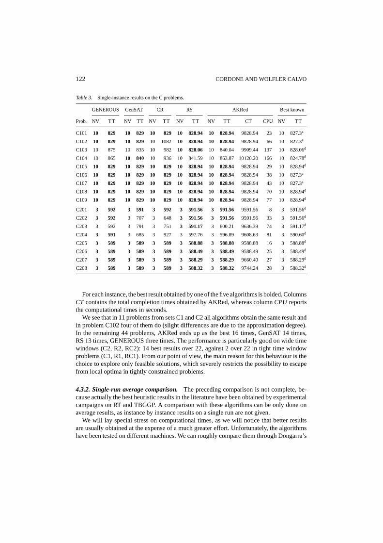
Table 3. Single-instance results on the C problems.



C101 10 829 10 829 10 829 10 828.94 10 828.949828.94 23 10 827.3a

C102 10 829 10 829 10 1082 10 828.94 10 828.94 9828.94 66 10 827.3a

C103 10 875 10 835 10 98210 828.06 10 840.04 9909.44 137 10 828.06d

C104 10 865 10 840 10 936 10 841.59 10 863.87 10120.20 166 10 824.78d

C105 10 829 10 829 10 829 10 828.94 10 828.949828.94 29 10 828.94d

C106 10 829 10 829 10 829 10 828.94 10 828.949828.94 38 10 827.3a

C107 10 829 10 829 10 829 10 828.94 10 828.949828.94 43 10 827.3a

C108 10 829 10 829 10 829 10 828.94 10 828.949828.94 70 10 828.94d

C109 10 829 10 829 10 829 10 828.94 10 828.949828.94 77 10 828.94d

C201 3 592 3 591 3 592 3 591.56 3 591.569591.56 8 3 591.56d

C202 3 592 3 707 3 648 3 591.56 3 591.56 9591.56 33 3 591.56d

C203 3 592 3 791 3 751 3 591.17 3 600.21 9636.39 74 3 591.17d

C204 3 591 3 685 3 927 3 597.76 3 596.89 9608.63 81 3 590.60d

C205 3 589 3 589 3 589 3 588.88 3 588.889588.88 16 3 588.88d

C206 3 589 3 589 3 589 3 588.49 3 588.499588.49 25 3 588.49d

C207 3 589 3 589 3 589 3 588.29 3 588.299660.40 27 3 588.29d

C208 3 589 3 589 3 589 3 588.32 3 588.329744.24 28 3 588.32d

For each instance, the best result obtained by one of the five algorithms is bolded. ColumnsCT contains the total completion times obtained by AKRed, whereas columnCPU reportsthe computational times in seconds.

We see that in 11 problems from sets C1 and C2 all algorithms obtain the same result andin problem C102 four of them do (slight differences are due to the approximation degree).In the remaining 44 problems, AKRed ends up as the best 16 times, GenSAT 14 times,RS 13 times, GENEROUS three times. The performance is particularly good on wide timewindows (C2, R2, RC2): 14 best results over 22, against 2 over 22 in tight time windowproblems (C1, R1, RC1). From our point of view, the main reason for this behaviour is thechoice to explore only feasible solutions, which severely restricts the possibility to escapefrom local optima in tightly constrained problems.

4.3.2. Single-run average comparison.The preceding comparison is not complete, be-cause actually the best heuristic results in the literature have been obtained by experimentalcampaigns on RT and TBGGP. A comparison with these algorithms can be only done onaverage results, as instance by instance results on a single run are not given.

We will lay special stress on computational times, as we will notice that better resultsare usually obtained at the expense of a much greater effort. Unfortunately, the algorithmshave been tested on different machines. We can roughly compare them through Dongarra’s


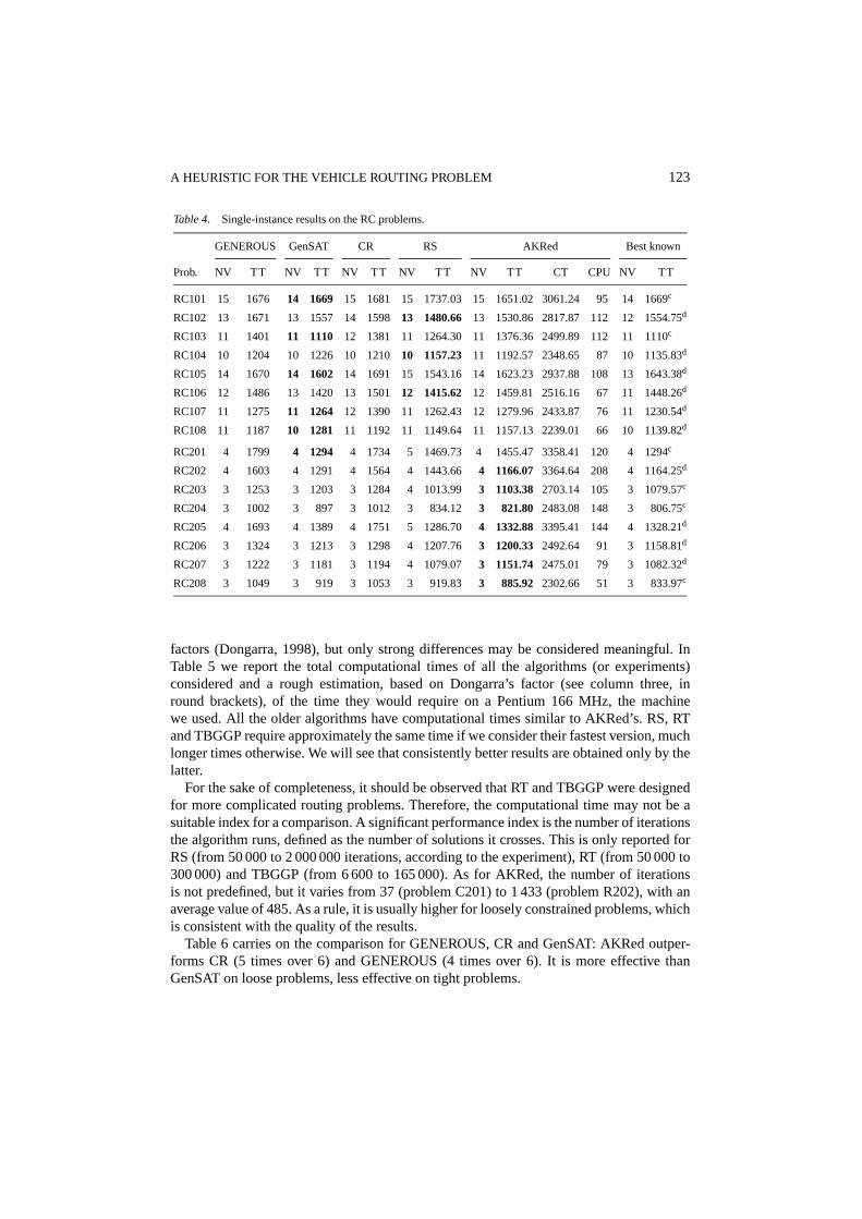
Table 4. Single-instance results on the RC problems.



RC101 15 1676 14 1669 15 1681 15 1737.03 15 1651.02 3061.24 95 14 1669c

RC102 13 1671 13 1557 14 159813 1480.66 13 1530.86 2817.87 112 12 1554.75d

RC103 11 1401 11 1110 12 1381 11 1264.30 11 1376.36 2499.89 112 11 1110c

RC104 10 1204 10 1226 10 121010 1157.23 11 1192.57 2348.65 87 10 1135.83d

RC105 14 1670 14 1602 14 1691 15 1543.16 14 1623.23 2937.88 108 13 1643.38d

RC106 12 1486 13 1420 13 150112 1415.62 12 1459.81 2516.16 67 11 1448.26d

RC107 11 1275 11 1264 12 1390 11 1262.43 12 1279.96 2433.87 76 11 1230.54d

RC108 11 1187 10 1281 11 1192 11 1149.64 11 1157.13 2239.01 66 10 1139.82d

RC201 4 1799 4 1294 4 1734 5 1469.73 4 1455.47 3358.41 120 4 1294c

RC202 4 1603 4 1291 4 1564 4 1443.664 1166.07 3364.64 208 4 1164.25d

RC203 3 1253 3 1203 3 1284 4 1013.993 1103.38 2703.14 105 3 1079.57c

RC204 3 1002 3 897 3 1012 3 834.123 821.80 2483.08 148 3 806.75c

RC205 4 1693 4 1389 4 1751 5 1286.704 1332.88 3395.41 144 4 1328.21d

RC206 3 1324 3 1213 3 1298 4 1207.763 1200.33 2492.64 91 3 1158.81d

RC207 3 1222 3 1181 3 1194 4 1079.073 1151.74 2475.01 79 3 1082.32d

RC208 3 1049 3 919 3 1053 3 919.833 885.92 2302.66 51 3 833.97c

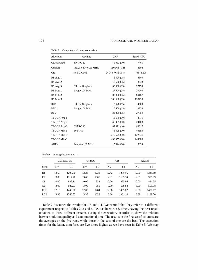
factors (Dongarra, 1998), but only strong differences may be considered meaningful. InTable 5 we report the total computational times of all the algorithms (or experiments)considered and a rough estimation, based on Dongarra’s factor (see column three, inround brackets), of the time they would require on a Pentium 166 MHz, the machinewe used. All the older algorithms have computational times similar to AKRed’s. RS, RTand TBGGP require approximately the same time if we consider their fastest version, muchlonger times otherwise. We will see that consistently better results are obtained only by thelatter.

For the sake of completeness, it should be observed that RT and TBGGP were designedfor more complicated routing problems. Therefore, the computational time may not be asuitable index for a comparison. A significant performance index is the number of iterationsthe algorithm runs, defined as the number of solutions it crosses. This is only reported forRS (from 50 000 to 2 000 000 iterations, according to the experiment), RT (from 50 000 to300 000) and TBGGP (from 6 600 to 165 000). As for AKRed, the number of iterationsis not predefined, but it varies from 37 (problem C201) to 1 433 (problem R202), with anaverage value of 485. As a rule, it is usually higher for loosely constrained problems, whichis consistent with the quality of the results.

Table 6 carries on the comparison for GENEROUS, CR and GenSAT: AKRed outper-forms CR (5 times over 6) and GENEROUS (4 times over 6). It is more effective thanGenSAT on loose problems, less effective on tight problems.


Table 5. Computational times comparison.

Algorithm Machine CPU Stand. CPU

GENEROUS SPARC 10 8 953 (10) 7461

GenSAT NeXT 68040 (25 MHz) 110 668 (1.4) 8608

CR 486 DX2/66 24 043 (0.56–2.4) 748–3 206

RS Avg-1 5 520 (15) 4600

RS Avg-2 16 600 (15) 13833

RS Avg-3 Silicon Graphics 33 300 (15) 27750

RS Min-1 Indigo 100 MHz 27 600 (15) 23000

RS Min-2 83 000 (15) 69167

RS Min-3 166 500 (15) 138750

RT-1 Silicon Graphics 5 520 (15) 4600

RT-2 Indigo 100 MHz 16 600 (15) 13833

RT-3 33 300 (15) 27750

TBGGP Avg-1 15 679 (10) 8711

TBGGP Avg-2 43 935 (10) 24408

TBGGP Avg-3 SPARC 10 87 871 (10) 48817

TBGGP Min-1 50 MHz 78 395 (10) 43553

TBGGP Min-2 219 675 (10) 122041

TBGGP Min-3 439 355 (10) 244086

AKRed Pentium 166 MHz 5 324 (18) 5324

Table 6. Average best results—1.

GENEROUS GenSAT CR AKRed

Prob. NV TT NV TT NV TT NV TT

R1 12.58 1296.80 12.33 1238 12.42 1289.95 12.50 1241.89

R2 3.00 1117.70 3.00 1005 2.91 1135.14 2.91 995.39

C1 10.00 838.11 10.00 832 10.00 885.86 10.00 834.05

C2 3.00 589.93 3.00 650 3.00 658.88 3.00 591.78

RC1 12.13 1446.20 12.00 1284 12.38 1455.82 12.38 1408.87

RC2 3.38 1360.57 3.38 1229 3.38 1361.14 3.38 1139.70

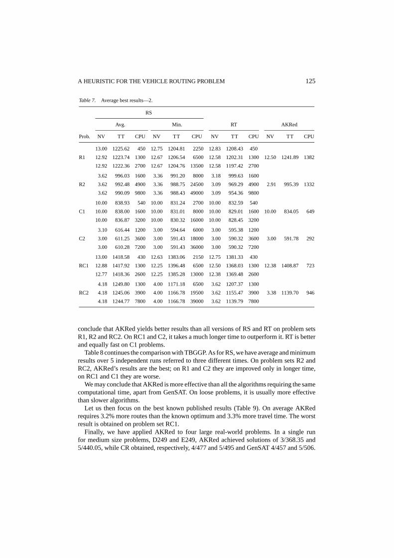
Table 7 discusses the results for RS and RT. We remind that they refer to a differentexperiment respect to Tables 2, 3 and 4: RS has been run 5 times, saving the best resultobtained at three different instants during the execution, in order to show the relationbetween solution quality and computational time. The results in the first set of columns arethe averages on the five runs, while those in the second one are the best. The executiontimes for the latter, therefore, are five times higher, as we have seen in Table 5. We may



RS

Avg. Min. RT AKRed

Prob. NV TT CPU NV TT CPU NV TT CPU NV TT CPU

13.00 1225.62 450 12.75 1204.81 2250 12.83 1208.43 450

R1 12.92 1223.74 1300 12.67 1206.54 6500 12.58 1202.31 1300 12.50 1241.89 1382

12.92 1222.36 2700 12.67 1204.76 13500 12.58 1197.42 2700

3.62 996.03 1600 3.36 991.20 8000 3.18 999.63 1600

R2 3.62 992.48 4900 3.36 988.75 24500 3.09 969.29 4900 2.91 995.39 1332

3.62 990.09 9800 3.36 988.43 49000 3.09 954.36 9800

10.00 838.93 540 10.00 831.24 2700 10.00 832.59 540

C1 10.00 838.00 1600 10.00 831.01 8000 10.00 829.01 1600 10.00 834.05 649

10.00 836.87 3200 10.00 830.32 16000 10.00 828.45 3200

3.10 616.44 1200 3.00 594.64 6000 3.00 595.38 1200

C2 3.00 611.25 3600 3.00 591.43 18000 3.00 590.32 3600 3.00 591.78 292

3.00 610.28 7200 3.00 591.43 36000 3.00 590.32 7200

13.00 1418.58 430 12.63 1383.06 2150 12.75 1381.33 430

RC1 12.88 1417.92 1300 12.25 1396.48 6500 12.50 1368.03 1300 12.38 1408.87 723

12.77 1418.36 2600 12.25 1385.28 13000 12.38 1369.48 2600

4.18 1249.80 1300 4.00 1171.18 6500 3.62 1207.37 1300

RC2 4.18 1245.06 3900 4.00 1166.78 19500 3.62 1155.47 3900 3.38 1139.70 946

4.18 1244.77 7800 4.00 1166.78 39000 3.62 1139.79 7800

conclude that AKRed yields better results than all versions of RS and RT on problem setsR1, R2 and RC2. On RC1 and C2, it takes a much longer time to outperform it. RT is betterand equally fast on C1 problems.

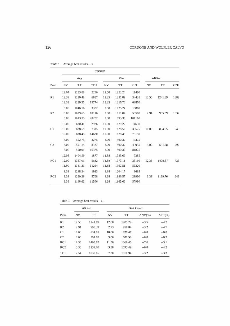
Table 8 continues the comparison with TBGGP. As for RS, we have average and minimumresults over 5 independent runs referred to three different times. On problem sets R2 andRC2, AKRed’s results are the best; on R1 and C2 they are improved only in longer time,on RC1 and C1 they are worse.

We may conclude that AKRed is more effective than all the algorithms requiring the samecomputational time, apart from GenSAT. On loose problems, it is usually more effectivethan slower algorithms.

Let us then focus on the best known published results (Table 9). On average AKRedrequires 3.2% more routes than the known optimum and 3.3% more travel time. The worstresult is obtained on problem set RC1.

Finally, we have applied AKRed to four large real-world problems. In a single runfor medium size problems, D249 and E249, AKRed achieved solutions of 3/368.35 and5/440.05, while CR obtained, respectively, 4/477 and 5/495 and GenSAT 4/457 and 5/506.



TBGGP

Avg. Min. AKRed

Prob. NV TT CPU NV TT CPU NV TT CPU

12.64 1233.88 2296 12.58 1222.24 11480

R1 12.39 1230.48 6887 12.25 1231.89 34435 12.50 1241.89 1382

12.33 1220.35 13774 12.25 1216.70 68870

3.00 1046.56 3372 3.00 1025.24 16860

R2 3.00 1029.65 10116 3.00 1011.04 50580 2.91 995.39 1332

3.00 1013.35 20232 3.00 995.38 101160

10.00 830.41 2926 10.00 829.22 14630

C1 10.00 828.59 7315 10.00 828.50 36575 10.00 834.05 649

10.00 828.45 14630 10.00 828.45 73150

3.00 592.75 3275 3.00 590.37 16375

C2 3.00 591.14 8187 3.00 590.37 40935 3.00 591.78 292

3.00 590.91 16375 3.00 590.30 81875

12.08 1404.59 1877 11.88 1385.69 9385

RC1 12.00 1387.01 5632 11.88 1373.11 28160 12.38 1408.87 723

11.90 1381.31 11264 11.88 1367.51 56320

3.38 1248.34 1933 3.38 1204.17 9665

RC2 3.38 1220.28 5798 3.38 1186.57 28990 3.38 1139.70 946

3.38 1198.63 11596 3.38 1165.62 57980


AKRed Best known

Prob. NV TT NV TT 1NV(%) 1TT(%)

R1 12.50 1241.89 12.08 1205.79 +3.5 +4.2

R2 2.91 995.39 2.73 958.84 +3.2 +4.7

C1 10.00 834.05 10.00 827.47 +0.0 +0.8

C2 3.00 591.78 3.00 589.59 +0.0 +0.3

RC1 12.38 1408.87 11.50 1366.45 +7.6 +3.1

RC2 3.38 1139.70 3.38 1093.49 +0.0 +4.2

TOT. 7.54 1030.65 7.30 1010.94 +3.2 +3.3


As for large size problems, D417 and E417, AKRed obtained 55/3788.55 and 55/4325.45,CR 55/4235 and 55/4397, GenSAT 54/4866 and 55/4149. Multiple experiments with RTattained solutions of 54/6264.80 and 54/7211.83, whereas an experimental campaign onTBGGP produced 55/3439.80 and 55/3707.10.

5. Conclusions

We have presented a heuristic to solve the Vehicle Routing Problem with Time Windows(AKRed). Our main aim was to show that, even if we do not exploit fashionable metaheuris-tics as Tabu Search, Simulated Annealing or Genetic Algorithms, competitive results canbe obtained in short time. It only takes a fine tuning of simple elements.

Full determinism and feasibility at all steps are AKRed’s main features. Its three nestedlevels consist ofAlternatingtwo objective functions, classicalK-exchangeand aReductionprocedure to reduce the number of routes.

AKRed’s results are often better than those obtained by the most recently publishedmetaheuristics and not far from the best in the literature, though obtained in shorter time. Incase time is not a limited resource, the neighbourhood used can be easily widened thanksto the general scheme to accomplish arc exchanges we have sketched in Section 3.4. In theend, this algorithm can be easily embedded in an intensification and diversification schemesuch as those that have produced the best known results in the literature. This is likely toproduce interesting improvements.

Future work will be dedicated to apply the AKRed method to other problems, such as theCapacitated Vehicle Routing Problem (CVRP). Since almost all of its features are generalenough to be easily extended, most of the effort should be devoted to define an effectiveproblem-specific second objective function.

Acknowledgments

The authors would like to thank the anonymous referees for improving the quality of thepaper with their precious and careful remarks.

Note

1. Experience proves that optimising first with respect tow, instead ofz, leads on average to better results. Thoughinteresting, this phenomenon could simply depend on the data.

References

Baker, E.K. and J.R. Shaffer. (1986). “Solution Improvement Heuristic for the Vehicle Routing and SchedulingProblem with Time Window Constrainats.”American Journal of Mathematical and Managenent Sciences6,261–300.


Chiang, W.-C. and R. Russell. (1996). “Simulated Annealing Metaheuristics for the Vehicle Routing Problem withTime Windows.”Annals of Operations Research63, 1–29.

Cordone, R. and R. Wolfler Calvo. (1996). “Note About Time Window Constraints in Routin Problems.” InternalReport 96-005, Dipartimento di Elettronica e Informazione, Politecnico di Milano, Milano (Submitted).

Desrochers, M., J. Desrosiers, and M.M. Solomon. (1992). “A New Optimization Algorithm for the VehicleRouting Problem with Time Windows.”Operations Research40(2), 342–354.

Desrosiers, J., Y. Dumas, M.M.Solomon, and F. Soumis. (1995). “Time Constrained Routing and Scheduling.”In Handbooks in Operations Research and Management Science, Vol. 8: Network Routing, North-Holland,pp. 35–139.

Dongarra, J.J. (1998). “Performance of Various Computers Using Standard Linear Equations Software.” ReportCS-89-85, Computer Science Departement, University of Tennesse.

Fisher, M.L. and R. Jaikumar. (1981). “A Generalized Assignment Heuristic for the Vehicle Routing Problem.”Networks11, 109–124.

Fisher, M.L., K.O. Jornsten, and O.B.G. Madsen. (1997). “Vehicle Routing with Time Windows–Two OptimizationAlgorithms.” Operations Research45, 488–492.

Healy, P. and R. Moll. (1995). “A New Extension of Local Search Applied to the Dial-a-Ride Problem.”EuropeanJournal of Operational Research83, 83–104.

Kindervater, G.A.P. and M.W.P. Savelsbergh. (1997). “Vehicle Routing: Handling Edge Exchanges.” InLocalSearch in Combinatorial Optimization. Chichester: Wiley, pp. 337–360.

Kohl, N., J. Desrosiers, O.B.G. Madsen, M.M. Solomon, and F. Soumis. (1997). “K -path Cuts for the VehicleRouting Problem with Time Windows.” Technical Report 1997-12, Department of Mathematical Modelling,The Technical University of Denmark.

Kohl, N. and O.B.G. Madsen. (1997). “An Optimization Algorithm for the Vehicle Routing Problem with TimeWindows Based on Lagrangean Relaxation.”Operations Research45, 395–406.

Kolen, A.W.J., A.H.G. Rinnooy Kan, and H.W.J.M. Trienekens. (1997). “Vehicle Routing with Time Windows.”Operations Research35, 266–273.

Kontoravdis, G. and J.F. Bard. (1995). “A GRASP for the Vehicle Routing Problem with Time Windows.”ORSAJournal on Computing7, 10–23.

Lin, S. (1965). “Computer Solutions to the Travelling Salesman Problem.”Bell System Technical Journal44,2245–2269.

Lin, S. and B.W. Kernighan. (1973). “An Effective Heuristic Algorithm for the Travelling Salesman Problem.”Operations Research21, 498–516.

Or, I. (1976). “Traveling Salesman Type Combinatorial Problems and Their Relation to the Logistics of BloodBanking.” Ph.D. thesis, Department of Industrial Engineering and Management Sciences, Northwestern Uni-versity, Evanston, Illinois.

Potvin, J.Y. and S. Bengio. (1996). “The Vehicle Routing Problem with Time Windows—Part II: Genertic Search.”INFORMS Journal of Coputing8, 165–172.

Potvin, J.Y., T. Kervahut, B.L. Garcia, and J.M. Rousseau. (1996).“The Vehicle Routing Problem with TimeWindows—Part I: Tabu Search.”INFORMS Journal of Computing8, 158–164.

Potvin, J.Y. and J.M. Rousseau. (1993). “A Parallel Route Building Algorithm for the Vehicle Routing andScheduling Problem with Time Windows.”European Journal of Operational Research66, 331–340.

Rochat, Y. and F. Semet. (1994). “A Tabu Search Approach for Delivering Pet Food and Flour in Switzerland.”Journal of Operational Research Society45, 1233–1246.

Rochat, Y. and E.D. Taillard. (1995). “Probabilistic Diversification and Intensification in Local Search for VehicleRouting.”Journal of Heuristics1, 147–167.

Russell, R.A. (1977). “An Effective Heuristic for the m-Tour Travelling Salesman Problem with Some SideConditions.”Operation Research25, 517–524.

Russell, R.A. (1995). “Hybrid Heuristics for the Vehicle Routing Problems with Time Windows.”TransportationScience29, 156–166.

Savelsbergh, M.W.P. (1985). “Local Search in Routing Problems with Time Windows.”Annals of OperationsResearch4, 285–305.

Solomon, M.M. (1987). “Algorithms for the Vehicle Routing and Scheduling Problems with Time Window Con-straints.”Operations Research35, 254–265.


Taillard, E.D., P. Badeau, M. Gendreau, F. Guertin, and J.Y. Potvin. (1997). “A Tabu Search Heuristic for theVehicle Routing Problem with Time Windows.”Transportation Science31, 170–186.

Thangiah, S.R., I.H. Osman, and T. Sun. (1994). “Hybrid Genetic Algorithm, Simulated Annealing and TabuSearch Methods for Vehicle Routing Problem with Time Windows.” Technical Report 27, Computer Sci-ence Department, Slippery Rock University (Forthcoming in theAnnals of OR Transportation, Laporte andGendreau, eds.).

A Heuristic for the Vehicle Routing Problem with Time Windows

Documents