A Heterogeneous and Distributed Co-Simulation Environment

A Heterogeneous and Distributed Co-Simulation Environment

Alexandre Amory, Fernando Moraes, Leandro Oliveira, Ney Calazans, Fabiano HesselPontifícia Universidade Católica do Rio Grande do Sul (FACIN-PUCRS)

Av. Ipiranga, 6681 - Prédio 30 / BLOCO 4 - 90619-900 - Porto Alegre – RS – BRASIL{amory, moraes, laugusto, calazans, hessel}@inf.pucrs.br

Abstract

This paper presents the implementation andevaluation of a hardware and software co-simulation tool.Different simulators, which can be geographicallydistributed, compose this environment. Thecommunication between simulators is done using a co-simulation backplane. The co-simulation backplane readsa file describing how the modules are connected,automatically launches the simulators and controls thesimulation process. A case study is used as a benchmarkto validate the implementation and to evaluate the systemperformance using different hardware-software partitions.

1. Introduction

Complex embedded systems require the design ofhardware, software and, in some situations, analog devicesand mechanical parts, too. Different languages and modelsof computation (MOC) may be used to describe thesedomains. This kind of system is characterized as a multi-language heterogeneous system [2],[3]. On the other hand,there is the homogeneous approach, where a singlelanguage or MOC is used to describe all types of modules[2],[3]. The main limitation of such approach is theabsence of a language able to express the semantics of allMOCs related to a generic embedded system. Someapproaches propose to add specific libraries to supportMOCs not easily modeled with the chosen languageconstructs (e.g. SystemC). The heterogeneous multi-language model approach, used in this work, keeps theconceptual differences of each domain, describing eachmodule of the system using an appropriate and possiblyspecific language. The main challenge of this approach isto define a mechanism to control and synchronize theinteraction between heterogeneous modules describedusing distinct formalisms.

The current practice of system design the differentmodules of a heterogeneous system are usually designedand validated separately. When the overall systemfunctionality has to be validated, this approach may not bepossible for a system-on-a-chip design.

Figure 1 presents different levels where co-simulationcan be performed. At the system level, the main goal is tocharacterize the system functionality. At this level, thesoftware part of the system is described using aprogramming language, such as C or C++. The hardwarepart is described using a hardware description language,such as VHDL or Verilog. The communication protocolbetween hardware and software is abstracted at this level.At the architectural level the hardware/softwarecommunication is taken into account together with thetarget device. At the cycle-level simulation, the softwarecomponents are simulated using the binary code runningon a cycle level simulator of the target processor at thehost machine. The hardware components are simulated atRTL level, with possibly back-annotated physicalparasitic components.

SUBSYSTEM 1 ... SUBSYSTEM N

System LevelCo-simulation

CODESIGN TOOL

Software (C) Hardware (VHDL)

Architecture LevelCo-simulation

BinaryCode

ProcessorModel

SOFTWARE

RTL Model(VHDL RTL)

HARDWARE

PROTOTYPE

Cycle LevelCo-simulation

Figure 1. Co-design flow, highlighting co-simulation atdifferent abstraction levels [2].

Proceedings of the 15 th Symposium on Integrated Circuits and Systems Design (SBCCI’02) 0-7695-1807-9/02 $17.00 © 2002 IEEE

Therefore, the task of a co-simulation tool is twofold:(i) to validate through simulation each module of thedesign, according to the language used to describe themodule (C, VHDL, JAVA, SDL, …); (ii) to manage thecommunication between different simulators. Formalverification tools are another possibility to validatehardware or software modules, but this approach is stillimmature [1].

This paper presents the implementation and evaluationof a geographically distributed co-simulation tool.Currently, this co-simulation tool validates heterogeneousdesigns at the system and RTL levels, with the softwarepart described in C/C++ and the hardware part describedin VHDL.

Different hardware/software partitions of a simplebenchmark are used to evaluate the tool in terms of CPUtime to fulfil the co-simulation in a Local Area Network(LAN) and in a Wide Area Network (WAN). The paperalso presents an evaluation of the CPU time spent withsimulation and communication. This analysis indicates theoverhead induced by the backplane, pointing out wherethe co-simulation can be improved.

The paper is organized as follows. Main conceptsrelated to co-simulation are presented in Section 2. InSection 3, the architecture of the co-simulationenvironment is introduced. The benchmark used tovalidate the tool and preliminary results is presented inSection 4. Finally, Section 5 provides some final remarksand presents possibilities for future work.

2. Co-simulation Classifications

2.1. Criterion: number of simulators

A homogeneous co-simulation model translates thedescription language of the modules composing thesystem to a single language, called intermediate format,able to describe the whole system. In this approach onlyone simulator is required.

A heterogeneous co-simulation model employs adedicated simulator for each language employed. In thisapproach, a backplane is required to coordinate thecommunication between simulators.

2.2. Criterion: simulation execution timing model

A functional model is used to validate the system athigher abstraction levels, where temporal andcommunication details are neglected.

A temporal model allows more accurate validation,since timing information, processor architecture and busmodel can be taken into account when simulators areinteracting. The common approach is to employ the sameglobal time for all simulators. This type of validation is

used to characterize the system at the cycle level and it islonger to simulate than the functional model.

2.3. Criterion: distributed and local co-simulation

The distributed co-simulation allows parallelexecution of simulators in geographically distributedmachines over a LAN or over a WAN. The benefits ofsuch approach are: (i) project decentralization; (ii) designand validation of a system under development bygeographically distributed teams; (iii) intellectual propertymanagement – a core provider may allow the simulationof an IP without giving out its description (source code);(iv) simulator's license management, since simulators canbe installed only in a few set of machines; (v) resourcesharing. The main drawback of this approach is theincrease in the co-simulation execution time, as a result ofthe network communication overhead introduced.

The local co-simulation has no communicationoverhead, as a network is not used for message exchange.On the other hand, it does not present the advantages ofdistributed co-simulation due to its lack of connectivity.

3. Architecture of the Co-simulationEnvironment

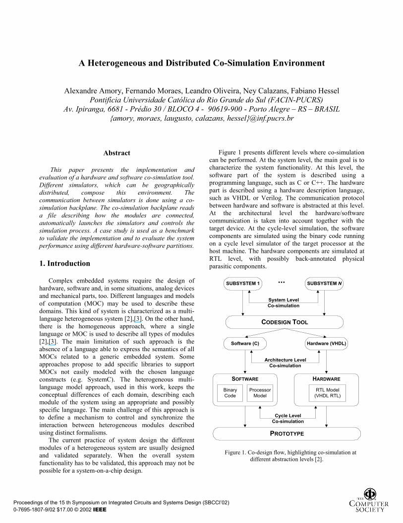
Figure 2 presents the main components of the co-simulation environment (light colored) and the userproject (dark colored). To use the environment the usermust add the appropriate communication library (ComLib)to each module. The description languages, C and VHDL,and the respective simulators, gcc and QuickHDL, musthave their own communication library. This figure will beused in the rest of the paper to describe the environment.

TestBench

User’sVHDLCommunication

Components

User’sC Code

ComLibVHDL

FLIComLibC

VHDLSimulator

CoordinationFileCo-simulation Backplane

Figure 2. General structure of the co-simulation environment.

Proceedings of the 15 th Symposium on Integrated Circuits and Systems Design (SBCCI’02) 0-7695-1807-9/02 $17.00 © 2002 IEEE

The ComLibC and ComLibVHDL are librariesresponsible for encapsulating the communicationsprimitives to the backplane. FLI is a VHDL extension toallow interfacing the VHDL simulator to the C language.The communication components obtained using theprimitives of the ComLibVHDL, and the user modules areinstantiated in the testbench. The communication betweenthe testbench and the C modules is coordinated by the co-simulation backplane.

3.1. Describing Modules for Co-Simulation

• Software ModulesSoftware modules are processes executing C code. In

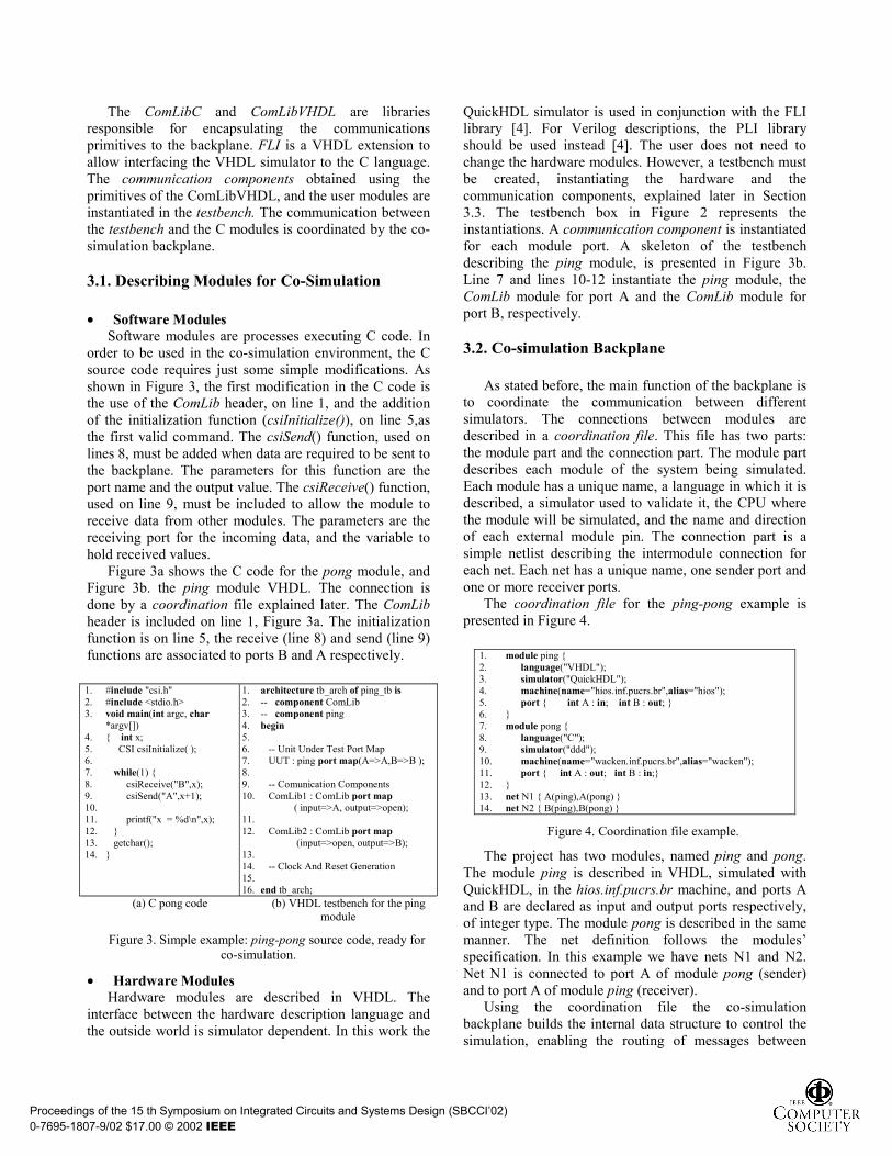
order to be used in the co-simulation environment, the Csource code requires just some simple modifications. Asshown in Figure 3, the first modification in the C code isthe use of the ComLib header, on line 1, and the additionof the initialization function (csiInitialize()), on line 5,asthe first valid command. The csiSend() function, used onlines 8, must be added when data are required to be sent tothe backplane. The parameters for this function are theport name and the output value. The csiReceive() function,used on line 9, must be included to allow the module toreceive data from other modules. The parameters are thereceiving port for the incoming data, and the variable tohold received values.

Figure 3a shows the C code for the pong module, andFigure 3b. the ping module VHDL. The connection isdone by a coordination file explained later. The ComLibheader is included on line 1, Figure 3a. The initializationfunction is on line 5, the receive (line 8) and send (line 9)functions are associated to ports B and A respectively.

1. #include "csi.h"2. #include <stdio.h>3. void main(int argc, char

*argv[])4. { int x;5. CSI csiInitialize( );6. 7. while(1) {8. csiReceive("B",x);9. csiSend("A",x+1);10. 11. printf("x = %d\n",x);12. }13. getchar();14. }

1. architecture tb_arch of ping_tb is2. -- component ComLib3. -- component ping4. begin5. 6. -- Unit Under Test Port Map7. UUT : ping port map(A=>A,B=>B );8. 9. -- Comunication Components10. ComLib1 : ComLib port map

( input=>A, output=>open);11. 12. ComLib2 : ComLib port map

(input=>open, output=>B);13. 14. -- Clock And Reset Generation15. 16. end tb_arch;

(a) C pong code (b) VHDL testbench for the pingmodule

Figure 3. Simple example: ping-pong source code, ready forco-simulation.

• Hardware ModulesHardware modules are described in VHDL. The

interface between the hardware description language andthe outside world is simulator dependent. In this work the

QuickHDL simulator is used in conjunction with the FLIlibrary [4]. For Verilog descriptions, the PLI libraryshould be used instead [4]. The user does not need tochange the hardware modules. However, a testbench mustbe created, instantiating the hardware and thecommunication components, explained later in Section3.3. The testbench box in Figure 2 represents theinstantiations. A communication component is instantiatedfor each module port. A skeleton of the testbenchdescribing the ping module, is presented in Figure 3b.Line 7 and lines 10-12 instantiate the ping module, theComLib module for port A and the ComLib module forport B, respectively.

3.2. Co-simulation Backplane

As stated before, the main function of the backplane isto coordinate the communication between differentsimulators. The connections between modules aredescribed in a coordination file. This file has two parts:the module part and the connection part. The module partdescribes each module of the system being simulated.Each module has a unique name, a language in which it isdescribed, a simulator used to validate it, the CPU wherethe module will be simulated, and the name and directionof each external module pin. The connection part is asimple netlist describing the intermodule connection foreach net. Each net has a unique name, one sender port andone or more receiver ports.

The coordination file for the ping-pong example ispresented in Figure 4.

1. module ping {2. language("VHDL");3. simulator("QuickHDL");4. machine(name="hios.inf.pucrs.br",alias="hios");5. port { int A : in; int B : out; }6. }7. module pong {8. language("C");9. simulator("ddd");10. machine(name="wacken.inf.pucrs.br",alias="wacken");11. port { int A : out; int B : in;}12. }13. net N1 { A(ping),A(pong) }14. net N2 { B(ping),B(pong) }

Figure 4. Coordination file example.

The project has two modules, named ping and pong.The module ping is described in VHDL, simulated withQuickHDL, in the hios.inf.pucrs.br machine, and ports Aand B are declared as input and output ports respectively,of integer type. The module pong is described in the samemanner. The net definition follows the modules’specification. In this example we have nets N1 and N2.Net N1 is connected to port A of module pong (sender)and to port A of module ping (receiver).

Using the coordination file the co-simulationbackplane builds the internal data structure to control thesimulation, enabling the routing of messages between

Proceedings of the 15 th Symposium on Integrated Circuits and Systems Design (SBCCI’02) 0-7695-1807-9/02 $17.00 © 2002 IEEE

modules. The integer data type is used by the backplane.The communication libraries implement the necessarydata conversion, as std_logic_vetcor to integer and vice-versa.

3.3. Communication Library

The communication library, ComLib, integrates asimulator to the backplane through UNIX sockets [7].This library has three functions: initialization(csiInitialize()), send data (csiSend()) and receive data(csiReceive()). The function csiInitialize() connects amodule to the backplane. It receives as parameters thename of the module to be simulated, and the backplane IPaddress. The sending and receiving functions receive twoparameters: the name of the port and the data to be sent orreceived.

At present, the environment supports only C/C++ andVHDL languages. It is important to add here that the Clibrary can also support C language variations as, forinstance, SystemC [5]. Libraries to support Java and SDLwill be implemented in a near future.

Figure 2 shows the structure of the C and VHDLlibraries. The C library, ComLib, could be seen as asimple overloading of standard functions to handlesockets in C. The VHDL simulator communicates withthe backplane using the communication components. Thecomponents are instantiated in the testbench to connecteach VHDL port to the backplane, as shown in Figure 3b,lines 10 and 12. The communication components areimplemented using the ComLib and a proprietary librarycalled FLI. This library allows implementing VHDLentities or functions in the C language.

3.4. Using the Co-simulation Environment

The first step to use the co-simulation environment isto change manually the user’s project adding the ComLibprimitives for initialization and send/receive. The nextstep is to describe the coordination file, including themodule’s name, the language, the machine where it willrun, the ports and the connection between modules. Nowthe backplane can be run. It launches automatically themodules and wait for connection of all the modules. Afterthis, the backplane starts the simulation.

4. Results

Validation was conducted using a simple case study.The case study is an algorithm to fill non-concavepolygons [6]. This algorithm has been chosen since itallows an easy description of different hardware-softwarepartitions and depending on the partitions thecommunication between blocks is very intensive (see field#msgs in Table 2), allowing the evaluation of the

communication overhead. This example may not be agood representative of the complexity found in genericembedded systems, but it was chosen as the objective hereis to show co-simulation problems.

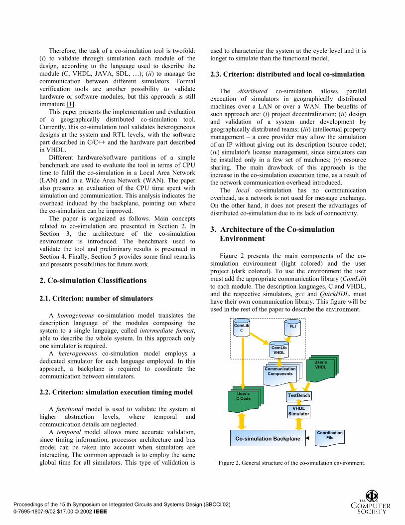
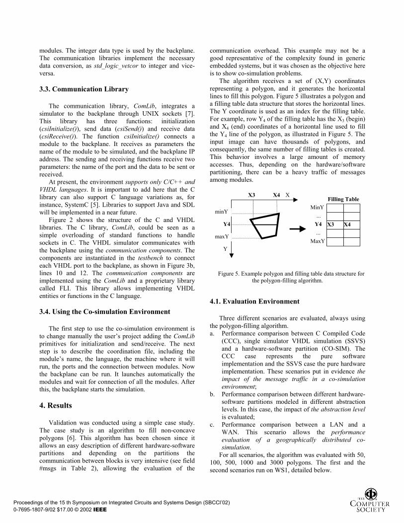
The algorithm receives a set of (X,Y) coordinatesrepresenting a polygon, and it generates the horizontallines to fill this polygon. Figure 5 illustrates a polygon anda filling table data structure that stores the horizontal lines.The Y coordinate is used as an index for the filling table.For example, row Y4 of the filling table has the X3 (begin)and X4 (end) coordinates of a horizontal line used to fillthe Y4 line of the polygon, as illustrated in Figure 5. Theinput image can have thousands of polygons, andconsequently, the same number of filling tables is created.This behavior involves a large amount of memoryaccesses. Thus, depending on the hardware/softwarepartitioning, there can be a heavy traffic of messagesamong modules.

minY

maxY

Y

X

X3 X4

X3 X4

Y4

MinY

Y4 ...MaxY

...

Filling Table

Figure 5. Example polygon and filling table data structure forthe polygon-filling algorithm.

4.1. Evaluation Environment

Three different scenarios are evaluated, always usingthe polygon-filling algorithm.a. Performance comparison between C Compiled Code

(CCC), single simulator VHDL simulation (SSVS)and a hardware-software partition (CO-SIM). TheCCC case represents the pure softwareimplementation and the SSVS case the pure hardwareimplementation. These scenarios put in evidence theimpact of the message traffic in a co-simulationenvironment;

b. Performance comparison between different hardware-software partitions modeled in different abstractionlevels. In this case, the impact of the abstraction levelis evaluated;

c. Performance comparison between a LAN and aWAN. This scenario allows the performanceevaluation of a geographically distributed co-simulation.

For all scenarios, the algorithm was evaluated with 50,100, 500, 1000 and 3000 polygons. The first and thesecond scenarios run on WS1, detailed below.

Proceedings of the 15 th Symposium on Integrated Circuits and Systems Design (SBCCI’02) 0-7695-1807-9/02 $17.00 © 2002 IEEE

For the third scenario, a set of 6 workstations was usedto validate the geographically distributed co-simulation:(1) WS1: Sun Ultra10, 333 MHz, 256 MB RAM; (2)WS2: Sun Ultra1, 167 MHz, 192 MB RAM; (3) WS3:Sun SPARC 4, 110 MHz, 72 MB RAM; (4) WS4: SunSPARC 4, 110 MHz, 72 MB RAM; (5) WS5: Sun SPARC4, 110 MHz, 64 MB RAM; (6) WS6: Sun Ultra2, 296MHz, 256 MB RAM.

The WS1 to WS5 boxes are connected on a LANEthernet 10Mbps. The WS6 is on a WAN 5 hops way. AllC programs were compiled using GNU GCC compilerversion 2.95.3 without optimization. The VHDL simulatorused in all experiments was Mentor Graphics QuickHdl(qhsim v8.5_4.6i). All data presented in the tablesrepresent average values, obtained through severalexecutions.

4.2. The Partitions

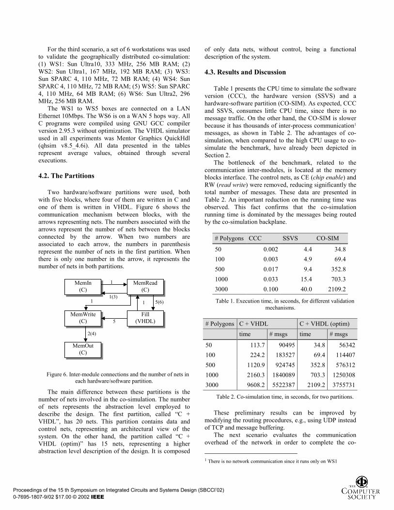
Two hardware/software partitions were used, bothwith five blocks, where four of them are written in C andone of them is written in VHDL. Figure 6 shows thecommunication mechanism between blocks, with thearrows representing nets. The numbers associated with thearrows represent the number of nets between the blocksconnected by the arrow. When two numbers areassociated to each arrow, the numbers in parenthesisrepresent the number of nets in the first partition. Whenthere is only one number in the arrow, it represents thenumber of nets in both partitions.

MemIn(C)

MemRead(C)

Fill(VHDL)

MemWrite(C)

MemOut(C)

1

1(3)

2(4)

5

1 5(6)1

Figure 6. Inter-module connections and the number of nets ineach hardware/software partition.

The main difference between these partitions is thenumber of nets involved in the co-simulation. The numberof nets represents the abstraction level employed todescribe the design. The first partition, called “C +VHDL”, has 20 nets. This partition contains data andcontrol nets, representing an architectural view of thesystem. On the other hand, the partition called “C +VHDL (optim)” has 15 nets, representing a higherabstraction level description of the design. It is composed

of only data nets, without control, being a functionaldescription of the system.

4.3. Results and Discussion

Table 1 presents the CPU time to simulate the softwareversion (CCC), the hardware version (SSVS) and ahardware-software partition (CO-SIM). As expected, CCCand SSVS, consumes little CPU time, since there is nomessage traffic. On the other hand, the CO-SIM is slowerbecause it has thousands of inter-process communication1

messages, as shown in Table 2. The advantages of co-simulation, when compared to the high CPU usage to co-simulate the benchmark, have already been depicted inSection 2.

The bottleneck of the benchmark, related to thecommunication inter-modules, is located at the memoryblocks interface. The control nets, as CE (chip enable) andRW (read write) were removed, reducing significantly thetotal number of messages. These data are presented inTable 2. An important reduction on the running time wasobserved. This fact confirms that the co-simulationrunning time is dominated by the messages being routedby the co-simulation backplane.

# Polygons CCC SSVS CO-SIM

50 0.002 4.4 34.8100 0.003 4.9 69.4500 0.017 9.4 352.81000 0.033 15.4 703.33000 0.100 40.0 2109.2

Table 1. Execution time, in seconds, for different validationmechanisms.

# Polygons C + VHDL C + VHDL (optim)time # msgs time # msgs

50 113.7 90495 34.8 56342100 224.2 183527 69.4 114407500 1120.9 924745 352.8 5763121000 2160.3 1840089 703.3 12503083000 9608.2 5522387 2109.2 3755731

Table 2. Co-simulation time, in seconds, for two partitions.

These preliminary results can be improved bymodifying the routing procedures, e.g., using UDP insteadof TCP and message buffering.

The next scenario evaluates the communicationoverhead of the network in order to complete the co-

1 There is no network communication since it runs only on WS1

Proceedings of the 15 th Symposium on Integrated Circuits and Systems Design (SBCCI’02) 0-7695-1807-9/02 $17.00 © 2002 IEEE

simulation. Table 3 presents the results for threeconfigurations. In the first one, all modules are executedin a single CPU, WS1. In the second case, the co-simulation is executed in 5 different CPUs (WS1 to WS5),belonging to the same LAN. In the third case, one externalCPU is added, WS6, replacing the WS5 of the previouscase. The CPUs are characterized at Section 4.2.

The total co-simulation time is almost the same in thethree cases: single machine, LAN and WAN. We couldexpect an improvement of the running time, sincesimulators are been executed in parallel. This is notobserved, because individual blocks are very simple,being quickly executed. So, the running time is again afunction of the number of messages being routed.

#Polygons

SingleMachine

Distributedonly LAN

DistributedLAN + WAN

50 34.8 41.0 36.3100 69.4 76.4 72.5500 352.8 423.1 368.11000 703.3 725.5 751.93000 2109.2 2177.4 2238.8

Table 3. Co-simulation time, in seconds, for singlemachine, LAN and WAN Co-simulation.

To put in evidence the reduction on the running timethe benchmarks must be CPU dominated, instead trafficdominated.

These results show us we can have distributedmodules over the network, with little impact on the overallrunning time, corroborating the advantages claimed forgeographically distributed simulation.

5. Conclusions And Future Work

The main contribution of this paper is the developmentand the evaluation of a co-simulation tool, by means a co-simulation backplane, responsible for the integration ofsimulators. The main features of the co-simulation toolare: (i) the co-simulation backplane automatically launchsimulators with no manual intervention; (ii)geographically distributed co-simulation is allowed; (iii)VHDL and C languages (as well as C variations) aresupported; (iv) functional and RTL architectural modelscan be used. Cycle level co-simulation is yet not

supported, since the backplane does not have a globalsynchronization mechanism.

One weakness of the currently implemented co-simulation environment is related to its lack of portability.The C/VHDL communication interface is not a standard,changing from simulator to simulator. The QuickHDLsimulator, used in this work, provides the FLI library. TheAldec simulator provides another library, called VHPI.So, if the VHDL simulator changes, some interfaces of thesystem must be re-written.

It is important to emphasize the backplane's flexibility.The backplane is independent from simulators. Newlanguages, such as Java and SDL, can easily be integratedin the co-simulation environment. The user only needs toimplement in these new languages the communicationlibrary.

As expected, the communication overhead was veryimportant. We believe this overhead can be reduced usingUDP sockets and message buffering. This optimization isunder development. Integration to Java and SDL and moredetailed performance evaluation benchmarks are examplesof future work.

As an academic work this environment can be freelydistributed to other research groups.

6. References

[1] Edwards, S., Lavagno, L., Lee, E., and Sangiovanni-vincentelli, A, "Design of Embedded Systems: FormalModels, Validation and Synthesis", Proceedings of theIEEE, 1997.

[2] Hessel, F., "Concepção de Sistemas Heterogêneos Multi-Linguagens", Jornada de Atualização em Informática –JAI, XXI Congresso da Sociedade Brasileira deComputação, 2001.

[3] Liem, C., Nacabal, F., Valderrama, C., Paulin, P., Jerraya,A., "System-on-a-chip Cosimulation and Compilation",IEEE Design & Test of Computers, Vol. 14, Issue 2, 1997,pp. 16 –25.

[4] Modeltech inc., "ModelSim SE/EE User’s Manual",Version 5.4. April, 2000.

[5] Swan, S., "An Introduction to System Level Modeling inSystemC 2.0", white paper, Available at homepage:http://www.systemc.org. 2001

[6] Foley, J.D., et al., Computer Graphics: Principles andPractice. 2 edn, Addison-Wesley, 1997.

[7] Walton,S., LINUX Socket Programming, SAMS, 2001.

Acknowledgements: Fernando Moraes gratefully acknowledges thesupport of the CNPq through research grant number 522939/96-1.

Proceedings of the 15 th Symposium on Integrated Circuits and Systems Design (SBCCI’02) 0-7695-1807-9/02 $17.00 © 2002 IEEE