A hardware-in-the-loop dynamics simulator for motorcycle rapid controller prototyping

Computers and Electronics in Agriculture 47 (2005) 41–58

Automatic velocity control of aself-propelled windrower

Christopher A. Fostera, Rick P. Strosserb, Jeremy Petersb,Jian-Qiao Suna,∗

a Department of Mechanical Engineering, University of Delaware, Newark, DE 19716, USAb Electrical Engineering Competency Center, CNH North America LLC, 500 Diller Avenue,

New Holland, PA 17557, USA

Received 1 June 2004; received in revised form 23 September 2004; accepted 8 October 2004

Abstract

A velocity control methodology is presented for an agricultural vehicle with a hydrostatic drive-train. A cascade control design incorporating a current control, cylinder position control and velocitycontrol is proposed. The cylinder position controller uses a set of gain scheduled lag compensators inseries with a sequence of segmented deadzone inversions. The deadzone inversions compensate fornonlinear valve dynamics. The velocity controller consists of a digital feedback control. A stabilityanalysis of the closed loop system is performed. Experimental results from a self-propelled windrowerare used to demonstrate the effectiveness of the control system.© 2004 Elsevier B.V. All rights reserved.

Keywords: Variable-structure feedback control; Segmented deadzone inversion; Autonomous vehicles; Vehiclevelocity control; Embedded controller

1. Introduction

In the past two decades the use of electronic control systems in vehicles has beensteadily increasing. Due to economies of scale the auto industry has lead the way in

∗ Corresponding author.E-mail address:[email protected] (J.-Q. Sun).

0168-1699/$ – see front matter © 2004 Elsevier B.V. All rights reserved.doi:10.1016/j.compag.2004.10.001

42 C.A. Foster et al. / Computers and Electronics in Agriculture 47 (2005) 41–58

the application of electronic controls on vehicles. Systems such as cruise-control, elec-tronic engine management, climate control and electronic transmissions are now commonin automobiles. In the last 10 years manufacturers of agricultural machinery have beendeveloping and releasing more electronic control systems on their equipment. Precisionagriculture is an area of research and development making extensive use of control sys-tems (Auernhammer, 2001; Earl et al., 2000; Zhang et al., 2002). Vehicle automationwith control systems is an important element of precision agriculture. The material pre-sented in this work demonstrates an automatic velocity control system for a self-propelledwindrower.

A significant research effort is being devoted to work on unmanned automated agricul-tural vehicles(Callaghan et al., 1997; Keicher and Seufert, 2000; Reid et al., 2000; Torii,2000). A fully automated vehicle has many interacting subsystems and will have sev-eral levels of control. The control objectives include vehicle motion, trajectory following,obstacle detection and tool manipulation.Stentz et al. (2002)have developed and testeda semi-autonomous tractor and sprayer for fleet applications in orchards. An ‘intelligentautonomous agricultural robot’ was developed and experimentally tested byHagras et al.(2002). The robot adjusts to changing and dynamic outdoor operating environments throughuse of a fuzzy-genetic control system. For this kind of technology to reach the marketplace,the cost has to be reasonable. Manufacturers of agricultural equipment will not fit these sys-tems to their products unless they are cost effective. This paper will present a cost effectivecontrol system for the windrower.

Automatic velocity control, known as ‘cruise-control’ in automobiles, has been availablefor quite sometime. Automobile drive-trains exhibit nonlinear dynamic behavior, particu-larly at lower speeds(Fritz, 1996). At higher speeds the behavior becomes more linear.Classical linear controls have been successful in the higher speed ranges. The emerg-ing technology of automated-highway-systems (AHS) calls for speed control systems thatwork over the full range of speeds(Rajamani and Shladover, 2001; Rajamani et al., 2000;Rajamani and Zhu, 2002). A variety of nonlinear and adaptive systems have been developedto address this issue(Fritz, 1996; Ishida, 1992; McMahon et al., 1990; Setlur et al., 2003).However, the dynamics of automobile drive-trains are different from those of the windrowerhydrostatic drive-train. Due to the larger mass of the windrower and the rougher terrain inwhich it operates, the control task in this work can be difficult.

Electrohydraulics has been a common type of actuation in power machinery. A key ele-ment in the windrower propulsion system proposed here is a proportional directional valve.A number of mathematical valve models have been presented in the literature.Vaughan andGamble (1996)have developed a single-input–single-output (SISO) model of a proportionalsolenoid valve. The model uses solenoid voltage to estimate the spool response.Elmer andGentle (2001)extended this model into a so called ‘parsimonious valve model’ by incorpo-rating a nonlinear model of the solenoid. These models require a number of accurate valveparameters.Ferreira et al. (2002)have developed semi-empirical model that predicts flowand pressure of a hydraulic servo-solenoid valve.Jelali and Schwarz (1995)andSchwarz(1998)have studied valve models in observer canonical form in which the spool position isused. In more expensive servo-valves, a linear-velocity-differential-transformer (LVDT) isused to measure the spool position and velocity. In many applications, where cost is a majorconcern, an LVDT may be too expensive. The models discussed above byVaughan and

C.A. Foster et al. / Computers and Electronics in Agriculture 47 (2005) 41–58 43

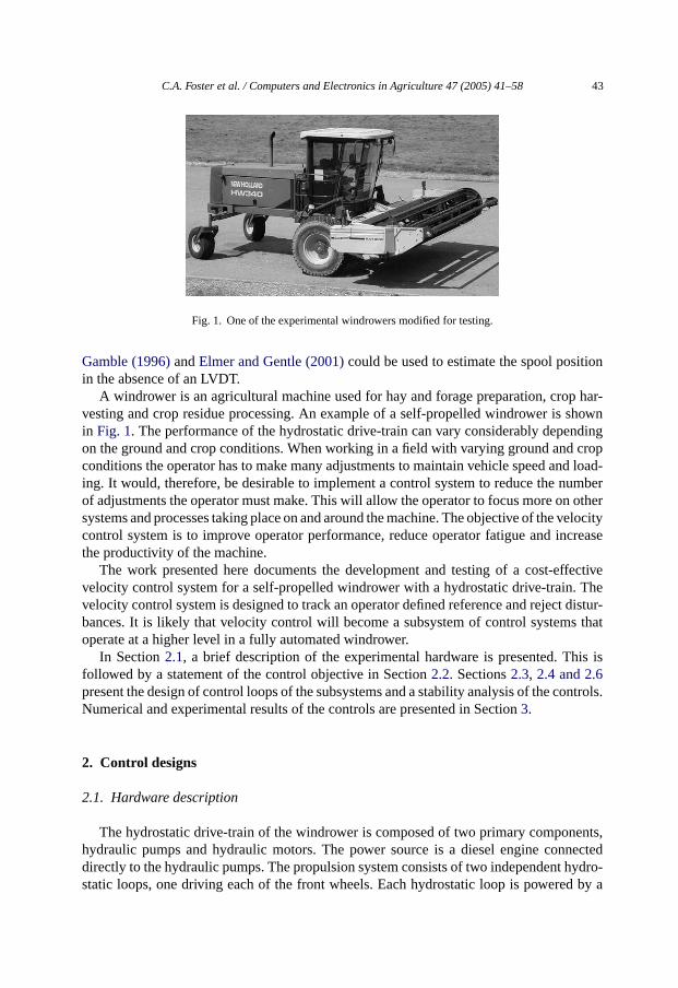
Fig. 1. One of the experimental windrowers modified for testing.

Gamble (1996)andElmer and Gentle (2001)could be used to estimate the spool positionin the absence of an LVDT.

A windrower is an agricultural machine used for hay and forage preparation, crop har-vesting and crop residue processing. An example of a self-propelled windrower is shownin Fig. 1. The performance of the hydrostatic drive-train can vary considerably dependingon the ground and crop conditions. When working in a field with varying ground and cropconditions the operator has to make many adjustments to maintain vehicle speed and load-ing. It would, therefore, be desirable to implement a control system to reduce the numberof adjustments the operator must make. This will allow the operator to focus more on othersystems and processes taking place on and around the machine. The objective of the velocitycontrol system is to improve operator performance, reduce operator fatigue and increasethe productivity of the machine.

The work presented here documents the development and testing of a cost-effectivevelocity control system for a self-propelled windrower with a hydrostatic drive-train. Thevelocity control system is designed to track an operator defined reference and reject distur-bances. It is likely that velocity control will become a subsystem of control systems thatoperate at a higher level in a fully automated windrower.

In Section2.1, a brief description of the experimental hardware is presented. This isfollowed by a statement of the control objective in Section2.2. Sections2.3, 2.4 and 2.6present the design of control loops of the subsystems and a stability analysis of the controls.Numerical and experimental results of the controls are presented in Section3.

2. Control designs

2.1. Hardware description

The hydrostatic drive-train of the windrower is composed of two primary components,hydraulic pumps and hydraulic motors. The power source is a diesel engine connecteddirectly to the hydraulic pumps. The propulsion system consists of two independent hydro-static loops, one driving each of the front wheels. Each hydrostatic loop is powered by a


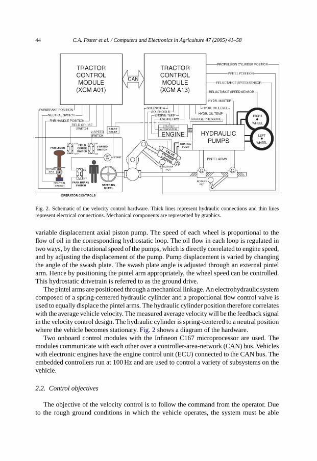
Fig. 2. Schematic of the velocity control hardware. Thick lines represent hydraulic connections and thin linesrepresent electrical connections. Mechanical components are represented by graphics.

variable displacement axial piston pump. The speed of each wheel is proportional to theflow of oil in the corresponding hydrostatic loop. The oil flow in each loop is regulated intwo ways, by the rotational speed of the pumps, which is directly correlated to engine speed,and by adjusting the displacement of the pump. Pump displacement is varied by changingthe angle of the swash plate. The swash plate angle is adjusted through an external pintelarm. Hence by positioning the pintel arm appropriately, the wheel speed can be controlled.This hydrostatic drivetrain is referred to as the ground drive.

The pintel arms are positioned through a mechanical linkage. An electrohydraulic systemcomposed of a spring-centered hydraulic cylinder and a proportional flow control valve isused to equally displace the pintel arms. The hydraulic cylinder position therefore correlateswith the average vehicle velocity. The measured average velocity will be the feedback signalin the velocity control design. The hydraulic cylinder is spring-centered to a neutral positionwhere the vehicle becomes stationary.Fig. 2shows a diagram of the hardware.

Two onboard control modules with the Infineon C167 microprocessor are used. Themodules communicate with each other over a controller-area-network (CAN) bus. Vehicleswith electronic engines have the engine control unit (ECU) connected to the CAN bus. Theembedded controllers run at 100 Hz and are used to control a variety of subsystems on thevehicle.

2.2. Control objectives

The objective of the velocity control is to follow the command from the operator. Dueto the rough ground conditions in which the vehicle operates, the system must be able


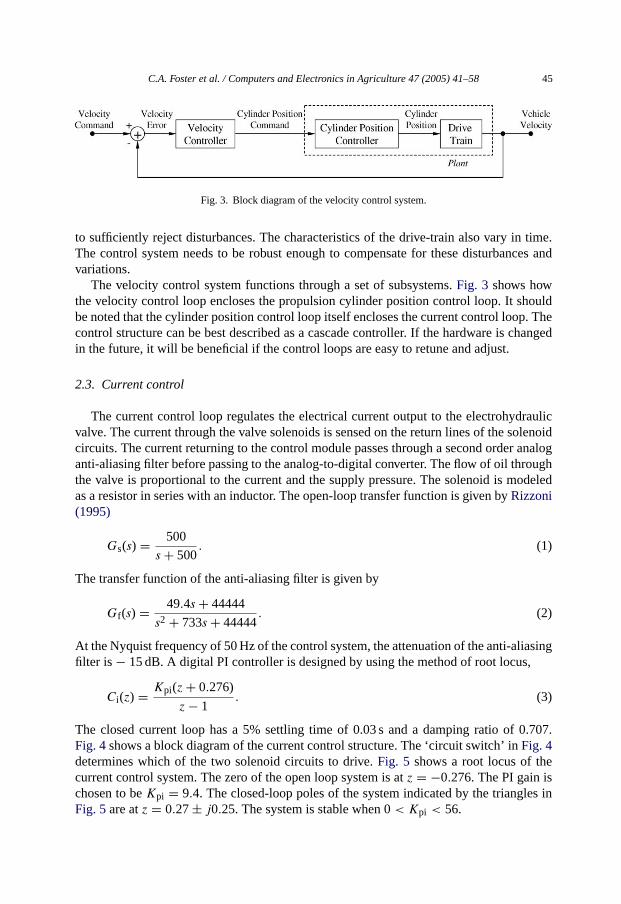
Fig. 3. Block diagram of the velocity control system.

to sufficiently reject disturbances. The characteristics of the drive-train also vary in time.The control system needs to be robust enough to compensate for these disturbances andvariations.

The velocity control system functions through a set of subsystems.Fig. 3 shows howthe velocity control loop encloses the propulsion cylinder position control loop. It shouldbe noted that the cylinder position control loop itself encloses the current control loop. Thecontrol structure can be best described as a cascade controller. If the hardware is changedin the future, it will be beneficial if the control loops are easy to retune and adjust.

2.3. Current control

The current control loop regulates the electrical current output to the electrohydraulicvalve. The current through the valve solenoids is sensed on the return lines of the solenoidcircuits. The current returning to the control module passes through a second order analoganti-aliasing filter before passing to the analog-to-digital converter. The flow of oil throughthe valve is proportional to the current and the supply pressure. The solenoid is modeledas a resistor in series with an inductor. The open-loop transfer function is given byRizzoni(1995)

Gs(s) = 500

s + 500. (1)

The transfer function of the anti-aliasing filter is given by

Gf (s) = 49.4s + 44444

s2 + 733s + 44444. (2)

At the Nyquist frequency of 50 Hz of the control system, the attenuation of the anti-aliasingfilter is − 15 dB. A digital PI controller is designed by using the method of root locus,

Ci (z) = Kpi(z + 0.276)

z − 1. (3)

The closed current loop has a 5% settling time of 0.03 s and a damping ratio of 0.707.Fig. 4shows a block diagram of the current control structure. The ‘circuit switch’ inFig. 4determines which of the two solenoid circuits to drive.Fig. 5 shows a root locus of thecurrent control system. The zero of the open loop system is atz = −0.276. The PI gain ischosen to beKpi = 9.4. The closed-loop poles of the system indicated by the triangles inFig. 5are atz = 0.27± j0.25. The system is stable when 0< Kpi < 56.


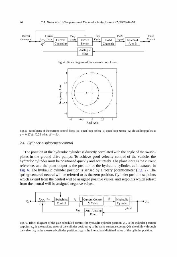
Fig. 4. Block diagram of the current control loop.

Fig. 5. Root locus of the current control loop: (×) open loop poles; (◦) open loop zeros; () closed loop poles atz = 0.27± j0.25 whenK = 9.4.

2.4. Cylinder displacement control

The position of the hydraulic cylinder is directly correlated with the angle of the swash-plates in the ground drive pumps. To achieve good velocity control of the vehicle, thehydraulic cylinder must be positioned quickly and accurately. The plant input is the currentreference, and the plant output is the position of the hydraulic cylinder, as illustrated inFig. 6. The hydraulic cylinder position is sensed by a rotary potentiometer (Fig. 2). Thespring-centered neutral will be referred to as the zero position. Cylinder position setpointswhich extend from the neutral will be assigned positive values, and setpoints which retractfrom the neutral will be assigned negative values.

Fig. 6. Block diagram of the gain scheduled control for hydraulic cylinder position:rcp is the cylinder positionsetpoint;ecp is the tracking error of the cylinder position;ri is the valve current setpoint;Q is the oil flow throughthe valve;ycp is the measured cylinder position;ycpf is the filtered and digitized value of the cylinder position.


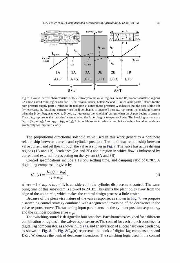
Fig. 7. Flow vs. current characteristics of the electrohydraulic valve: regions 1A and 1B, proportioanl flow; regions2A and 2B, dead zone; regions 3A and 3B, external influence. Letters ‘A’ and ‘B’ refer to the ports; P stands for thehigh pressure supply port; T refers to the tank port at atmospheric pressure; X indicates that the port is blocked;iBT represents the ‘cracking’ current when the B port begins to open to T port;iBp represents the ‘cracking’ currentwhen the B port begins to open to P port;iAt represents the ‘cracking’ current when the A port begins to open toT port; iAp represents the ‘cracking’ current when the A port begins to open to P port. The blocking currents areiAx = (iAp − iAt )/2 andiBx = (iBp − iBt)/2. A double solenoid valve is used but a single solenoid valve showngraphically for improved clarity.

The proportional directional solenoid valve used in this work generates a nonlinearrelationship between current and cylinder position. The nonlinear relationship betweenvalve current and oil flow through the valve is shown inFig. 7. The valve has active drivingregions (1A and 1B), deadzones (2A and 2B) and a region in which flow is influenced bycurrent and external forces acting on the system (3A and 3B).

Control specifications include a 1 s 5% settling time, and damping ratio of 0.707. Adigital lag compensator given by

Ccp(z) = Kcp(z + bcp)

(z + acp), (4)

where−1 ≤ acp < bcp ≤ 1, is considered in the cylinder displacement control. The sam-pling time of this subsystem is slowed to 20 Hz. This shifts the plant poles away from theedge of the unit circle, which makes the control design process a little easier.

Because of the piecewise nature of the valve response, as shown inFig. 7, we proposea switching control strategy combined with a segmented inversion of the deadzones in thevalve response curve. The switching input parameters are the cylinder position setpointrcpand the cylinder position errorecp.

The switching control is designed in four branches. Each branch is designed for a differentcombination of regions in the valve response curve. The control for each branch consists of adigital lag compensator, as shown in Eq.(4), and an inversion of a local hardware deadzone,as shown inFig. 8. In Fig. 8Ccp(n) represents the bank of digital lag compensators andDZinv(n) denotes the bank of deadzone inversions. The switching logic used in the control


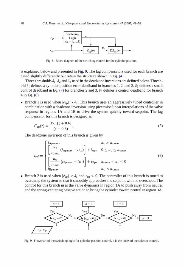
Fig. 8. Block diagram of the switching control for the cylinder position.

is explained below and presented inFig. 9. The lag compensators used for each branch aretuned slightly differently but retain the structure shown in Eq.(4).

Three thresholdsδ1, δ2 andδ3 used in the deadzone inversions are defined below. Thresh-old δ1 defines a cylinder position error deadband in branches 1, 2, and 3.δ2 defines a smallcontrol deadband in Eq.(7) for branches 2 and 3.δ3 defines a control deadband for branch4 in Eq.(8).

• Branch 1 is used when|ecp| > δ1. This branch uses an aggressively tuned controller incombination with a deadzone inversion using piecewise linear interpolations of the valveresponse in regions 1A and 1B to drive the system quickly toward setpoint. The lagcompensator for this branch is designed as

Ccp(z) = 35.1(z + 0.6)

(z − 0.8), (5)

The deadzone inversion of this branch is given by

iref =

iAp max, uc > uc max[uc

uc max(iAp max − iAp)

]+ iAp, 0 ≤ uc ≤ uc max[

uc

uc min

(iBp max− iBp

)]+ iBp, uc min ≤ uc ≤ 0

iBp max, uc < uc min

(6)

• Branch 2 is used when|ecp| < δ1 andrcp > 0. The controller of this branch is tuned tooverdamp the system so that it smoothly approaches the setpoint with no overshoot. Thecontrol for this branch uses the valve dynamics in region 1A to push away from neutraland the spring-centering passive action to bring the cylinder toward neutral in region 3A.

Fig. 9. Flowchart of the switching logic for cylinder position control.n is the index of the selected control.


The deadzone inversion is given by

iref =

iAp max, uc > uc max[(uc − δ2)

(uc max− δ2)(iAp max − iAp)

]+ iAp, δ2 ≤ uc ≤ uc max

iAx, |uc| < δ2[(uc + δ2)

(uc min − δ2)(iAt − iAt min)

]+ iAt, uc min ≤ uc ≤ −δ2

iAt min, uc < uc min

(7)

Notice that a small deadband exists to lock the cylinder in position using region 2A whenthe cylinder position error is sufficiently small. This deadband is adopted because thecylinder can only be positioned with a finite precision due to quantization errors, sensornoise, and hardware limitations.

• Branch 3 is used when|ecp| < δ1 and rcp < 0. This branch is similar to branch 2. Itincludes regions 1B, 2B and 3B. The lag compensator is tuned slightly differently toachieve performance similar to that in branch 2. This is because the volume flowratesof the oil associated with equivalent motion of the cylinder in each direction differ dueto the volume occupied by the connecting rod on one side of the piston. The deadzoneinversion in Eq.(7) is used with the ‘B’ current values substituted for the ‘A’ values.

• Branch 4 is used whenrcp = 0. The controller is tuned to bring the vehicle to a haltquickly. The lag compensator used is the same as shown in Eq.(5). The small deadbanduses the passive action of the spring to center the cylinder gently as it approaches theneutral position. The inversion mapping with a small deadband is given by

iref =

iAp max, uc > uc max[(uc − δ3)

(uc max− δ3)(iAp max − iAp)

]+ iAp, δ3 ≤ uc ≤ uc max

0, |uc| < δ3[(uc + δ3)

(uc min − δ3)(iBp max− iBp)

]− iBp, uc min ≤ uc ≤ −δ3

iBp max, uc < uc min

(8)

The cylinder position error deadband,δ1, is used to switch from branch 1 to either branch2 or 3. The reason for this is discussed in more detail in the remark below. The value ofδ1used in our experiments is 3 mm. The control deadbands,δ2 andδ3, are to stop the controluc when it drops below a certain level. The smaller the size of the deadband, the moreaccurately the controller will try to position the cylinder. A small deadband can also lead tochatter about the setpoint. The selection of the deadband size therefore has to balance thesetwo considerations. The value ofδ2 andδ3 used in our experiments is 1.5 mm.

In Eqs.(6)–(8),uc is the output of the lag compensator as shown inFig. 8. The parametersiAp, iAt, iBx, iBp, iBt andiBx are defined inFig. 7. The parametersiAp maxandiBp maxrepresentthe upper limits of the valve currents on the respective solenoids. The parametersiAt min andiBt min represent lower limits of the valve current on the respective solenoid. The parametersuc max anduc min are the limits of the control. All four of the inversion mappings have


saturation limits. Critical parameters of an individual valve are obtained from a calibrationprocedure.

Remark. The reason for switching control from branch 1 to either branch 2 or 3, as thesystem approaches the setpoint, is to eliminate oscillations about the setpoint that exist underthe control for branch 1. This phenomenon results from the fact that regions 1A and 1Breside on opposite sides ofFig. 7. When the system in branch 1 overshoots, it switches fromregion 1A to 1B. As this transition occurs, the system passes through all states in between.Recall that the hydraulic cylinder is spring-centered. As the system passes through regions3A and 3B on its way to region 1B, the cylinder will passively move toward the neutral.When the system crosses setpoint again, it switches back and hence once again passesthrough regions 3A and 3B. This causes the system to oscillate near the setpoint. Branches2 and 3 are implemented to prevent this from happening.

2.5. Cylinder position control stability analysis

2.5.1. Regions 1A and 1BWhen the valve is operating in regions 1A and 1B the hydraulic cylinder effectively

integrates the oil flow coming from the valve. The oil flow can be approximated as a linearfunction of the valve current minus the ‘cracking’ current (iAp or iBp). As shown inFig. 7this is due to the fact that only a small range of the valve capacity is used. An approximatemodel of the plant in these regions is given by,

ycpTKA1uc (9)

where the dot denotes differentiation with respect to time, andKA1 is a combined gainincluding the effects of the deadzone inversion, the current control and the cylinder positioncontrol. Branches 1 and 4 cover regions 1A and 1B. The output of the compensatoruc canhave both negative and positive values.

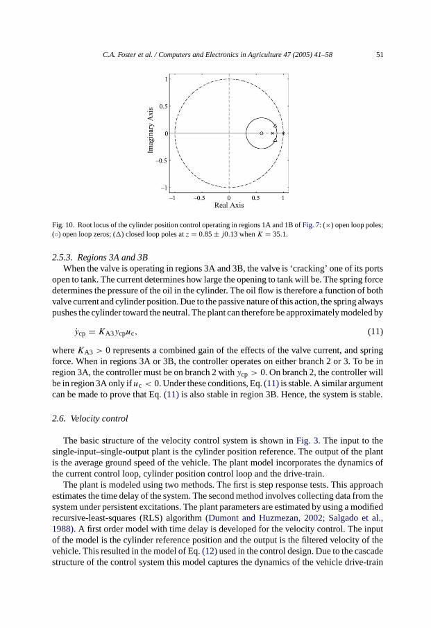
Fig. 10shows a root locus plot of the control system in regions 1A and 1B using Eq.(5) as the controller. The system is stable when 0< Kcp < 808. The closed-loop poles asshown inFig. 10have a damping ratio 0.707. The other branches have minor gain and pole-zero changes in the lag compensator but retain the same basic root locus profile. Hence, thesystem is stable in regions 1A and 1B.

2.5.2. Regions 2A and 2BIn regions 2A and 2B the oil flow is blocked, and the cylinder is locked in position. In

this state, we have

ycp = 0. (10)

In other words,ycp remains constant. The constant value ofycp is determined by the initialcondition upon entering either region 2A or 2B. The system in this state is marginally stablesince the hydraulic cylinder has hardware limits that preventycp from becoming unbounded.


Fig. 10. Root locus of the cylinder position control operating in regions 1A and 1B ofFig. 7: (×) open loop poles;(◦) open loop zeros; () closed loop poles atz = 0.85± j0.13 whenK = 35.1.

2.5.3. Regions 3A and 3BWhen the valve is operating in regions 3A and 3B, the valve is ‘cracking’ one of its ports

open to tank. The current determines how large the opening to tank will be. The spring forcedetermines the pressure of the oil in the cylinder. The oil flow is therefore a function of bothvalve current and cylinder position. Due to the passive nature of this action, the spring alwayspushes the cylinder toward the neutral. The plant can therefore be approximately modeled by

ycp = KA3ycpuc, (11)

whereKA3 > 0 represents a combined gain of the effects of the valve current, and springforce. When in regions 3A or 3B, the controller operates on either branch 2 or 3. To be inregion 3A, the controller must be on branch 2 withycp > 0. On branch 2, the controller willbe in region 3A only ifuc < 0. Under these conditions, Eq.(11)is stable. A similar argumentcan be made to prove that Eq.(11) is also stable in region 3B. Hence, the system is stable.

2.6. Velocity control

The basic structure of the velocity control system is shown inFig. 3. The input to thesingle-input–single-output plant is the cylinder position reference. The output of the plantis the average ground speed of the vehicle. The plant model incorporates the dynamics ofthe current control loop, cylinder position control loop and the drive-train.

The plant is modeled using two methods. The first is step response tests. This approachestimates the time delay of the system. The second method involves collecting data from thesystem under persistent excitations. The plant parameters are estimated by using a modifiedrecursive-least-squares (RLS) algorithm(Dumont and Huzmezan, 2002; Salgado et al.,1988). A first order model with time delay is developed for the velocity control. The inputof the model is the cylinder reference position and the output is the filtered velocity of thevehicle. This resulted in the model of Eq.(12)used in the control design. Due to the cascadestructure of the control system this model captures the dynamics of the vehicle drive-train


as well as the closed-loop dynamics of the cylinder position and current control loops.

Gv(s) = 6e−0.15s

0.85s + 1. (12)

The accuracy of the model can be evaluated using the index defined below

κ = 100

(1 −

∑(y − y)2∑

(y − µy)2

). (13)

whereκ lies in the range from 0 to 100,y is the measured plant output, ˆy is the simulatedplant output from the model,µy is the mean value of the measured output. Whenκ = 100,the model perfectly represents the physical plant. The value ofκ for the model in Eq.(12)is 78.9, which suggests a moderately high quality of fit.

The Zeigler–Nichols tuning rule is used to generate an initial set of proportional-integral-derivative (PID) control gains (Ogunnaike and Ray, 1994). The control gains are tunedfurther through simulation and again during implementation. It should be noted that thederivative control implemented uses the output derivative only, known as the tachome-tric derivative, excluding the unwanted derivative of the reference signal, thus allowingnonsmooth references. The result is that a zero is removed from the closed-loop transferfunction. This changes the stability margin as the relative degree of the closed-loop systemis increased by one. Since the transfer function in Eq.(12) captures the dyanmics of thecylinder position and current control loops, the stability of the velocity control loop impliesthe system stability. The control is given by

u(k) = up(k) + ui (k) + ud(k) (14a)

up(k) = Kpe(k) (14b)

ui (k) = KpTs

2τi(e(k) + e(k − 1)) + ui (k − 1) (14c)

ud(k) = −Kpτd

Ts(yv(k) − yv(k − 1)) (14d)

wheree(k) represents the error signal,yv(k) is the measured averaged velocity,Ts is thesample time,Kp is a control gain,τi is the integral time constant andτd is the derivative timeconstant. To prevent integral windup due to actuator saturation, the following conditionalintegration (CI) algorithm is used.

e(k) =

0, if(un �= us) and [(ui > ui max) or (ui < ui min)] andev(un − u) > 0,

ev(k), otherwise(14)

whereev(k) is the velocity error,us = sat(un, umin, umax) is the control with the saturationlimits umin andumax, un is the nominal control, ¯u = (umin + umax)/2, ui is the integral


Table 1Implemented velocity control gains

Proportional gain (Kp) 0.15Integral time constant (τd) 1.0Tachometric derivative time constant (τd) 0.4

control, andui max is the upper limit of the integral control. The closed-loop poles of thePID control with tachometric derivative are located atz = {−0.44, 0.96± 0.017} showingthat the system is stable.Table 1lists the implemented control gains.

3. Control simulations and experimental results

The control systems have been implemented and tested on prototype windrowers. Here,we present the simulation and experimental results on one windrower with ‘propulsion-by-wire’ capability. Some relevant parameters of the vehicle are listed inTable 2.

3.1. Current control

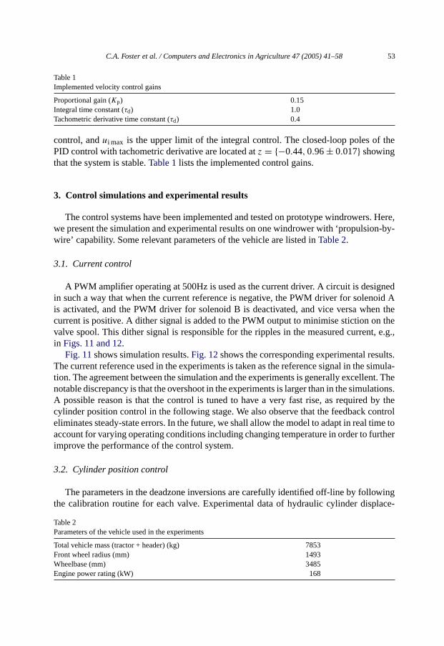
A PWM amplifier operating at 500Hz is used as the current driver. A circuit is designedin such a way that when the current reference is negative, the PWM driver for solenoid Ais activated, and the PWM driver for solenoid B is deactivated, and vice versa when thecurrent is positive. A dither signal is added to the PWM output to minimise stiction on thevalve spool. This dither signal is responsible for the ripples in the measured current, e.g.,in Figs. 11 and 12.

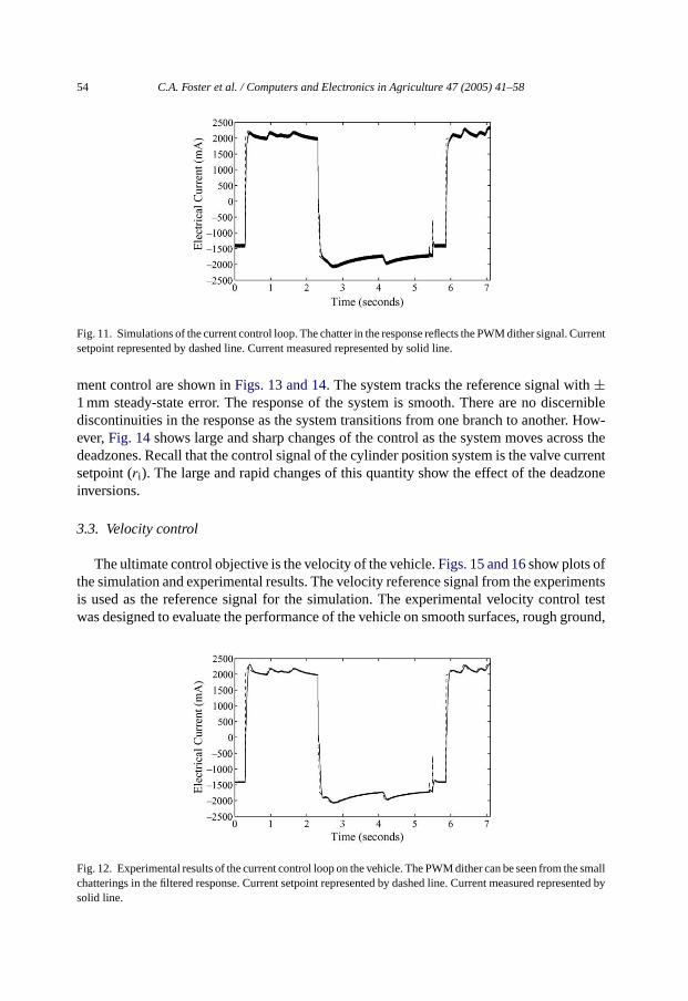
Fig. 11shows simulation results.Fig. 12shows the corresponding experimental results.The current reference used in the experiments is taken as the reference signal in the simula-tion. The agreement between the simulation and the experiments is generally excellent. Thenotable discrepancy is that the overshoot in the experiments is larger than in the simulations.A possible reason is that the control is tuned to have a very fast rise, as required by thecylinder position control in the following stage. We also observe that the feedback controleliminates steady-state errors. In the future, we shall allow the model to adapt in real time toaccount for varying operating conditions including changing temperature in order to furtherimprove the performance of the control system.

3.2. Cylinder position control

The parameters in the deadzone inversions are carefully identified off-line by followingthe calibration routine for each valve. Experimental data of hydraulic cylinder displace-

Table 2Parameters of the vehicle used in the experiments

Total vehicle mass (tractor + header) (kg) 7853Front wheel radius (mm) 1493Wheelbase (mm) 3485Engine power rating (kW) 168


Fig. 11. Simulations of the current control loop. The chatter in the response reflects the PWM dither signal. Currentsetpoint represented by dashed line. Current measured represented by solid line.

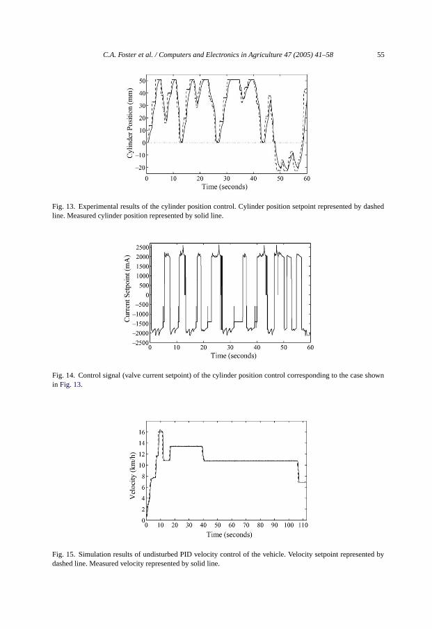
ment control are shown inFigs. 13 and 14. The system tracks the reference signal with±1 mm steady-state error. The response of the system is smooth. There are no discerniblediscontinuities in the response as the system transitions from one branch to another. How-ever,Fig. 14shows large and sharp changes of the control as the system moves across thedeadzones. Recall that the control signal of the cylinder position system is the valve currentsetpoint (ri ). The large and rapid changes of this quantity show the effect of the deadzoneinversions.

3.3. Velocity control

The ultimate control objective is the velocity of the vehicle.Figs. 15 and 16show plots ofthe simulation and experimental results. The velocity reference signal from the experimentsis used as the reference signal for the simulation. The experimental velocity control testwas designed to evaluate the performance of the vehicle on smooth surfaces, rough ground,

Fig. 12. Experimental results of the current control loop on the vehicle. The PWM dither can be seen from the smallchatterings in the filtered response. Current setpoint represented by dashed line. Current measured represented bysolid line.


Fig. 13. Experimental results of the cylinder position control. Cylinder position setpoint represented by dashedline. Measured cylinder position represented by solid line.

Fig. 14. Control signal (valve current setpoint) of the cylinder position control corresponding to the case shownin Fig. 13.

Fig. 15. Simulation results of undisturbed PID velocity control of the vehicle. Velocity setpoint represented bydashed line. Measured velocity represented by solid line.


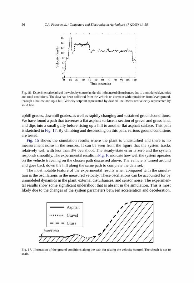
Fig. 16. Experimental results of the velocity control under the influence of disturbances due to unmodeled dynamicsand road conditions. The data has been collected from the vehicle on a terrain with transitions from level ground,through a hollow and up a hill. Velocity setpoint represented by dashed line. Measured velocity represented bysolid line.

uphill grades, downhill grades, as well as rapidly changing and sustained ground conditions.We have found a path that traverses a flat asphalt surface, a section of gravel and grass land,and dips into a small gully before rising up a hill to another flat asphalt surface. This pathis sketched inFig. 17. By climbing and descending on this path, various ground conditionsare tested.

Fig. 15 shows the simulation results where the plant is undisturbed and there is nomeasurement noise in the sensors. It can be seen from the figure that the system tracksrelatively well with less than 3% overshoot. The steady-state error is zero and the systemresponds smoothly. The experimental results inFig. 16indicate how well the system operateson the vehicle traveling on the chosen path discussed above. The vehicle is turned aroundand goes back down the hill along the same path to complete the data set.

The most notable feature of the experimental results when compared with the simula-tion is the oscillations in the measured velocity. These oscillations can be accounted for byunmodeled dynamics in the plant, external disturbances, and sensor noise. The experimen-tal results show some significant undershoot that is absent in the simulation. This is mostlikely due to the changes of the system parameters between acceleration and deceleration.

Fig. 17. Illustration of the ground conditions along the path for testing the velocity control. The sketch is not toscale.


Overall, the vehicle tracks a velocity command of 11.3 km/h with an error of approximately±0.5 km/h, or±4%. The uncontrolled system with a constant cylinder position provid-ing a velocity of 11.3 km/h on smooth level ground, gives an average tracking error ofapproximately±2.4 km/h, or±21% when following the same path.

4. Conclusion

This paper has presented an automatic velocity control system for a self-propelledwindrower. The control system has a cascade structure involving several subsystems. Inparticular, the control system includes a hydraulic valve with strongly nonlinear character-istics. A segmented inversion method of the valve nonlinear dynamics such as deadzone hasbeen developed for designing the cylinder position control. Stability of the control systemhas been proven. The control system has been tested and validated experimentally. Theexperimental results show that the velocity control system is stable, tracks the reference andrejects disturbances sufficiently well. The studies show that the techniques developed in thiswork provide an effective control solution for vehicles with nonlinear electromechanicalsubsystems. The control designed in this study is based on a static model of the plant. In thefuture the plant model will be allowed to adapt in real time to account for varying operationconditions. In this regard, this paper provides a foundation of such an extension. Finally,we point out that while this study has not considered wheel slippage, it can be a potentialproblem, and will be addressed in the future.

Acknowledgements

The authors would like to thank John Posselius, Leader of the Research and DevelopmentTeam at the CNH Technical Center, New Holland, Pennsylvania, for his support throughoutthe project. This work would not have been possible without the assistance of many peopleat the CNH Technical Center. We would especially like to thank members of the ElectricalEngineering Group and the New Generation Windrower Design Team for their help. Thehelp of Steve Paulin of Eaton hydraulics has been instrumental. Finally, we also recognizethe early contribution of Dr. James Glancey of the University of Delaware in the formationof the project.

References

Auernhammer, H., 2001. Precision farming—the environmental challenge. Comput. Electron. Agric. 30 (1–3),31–43.

Callaghan, V., Chernett, P., Colley, M., Lawson, T., Standeven, J., Carr-West, M., Ragget, M., 1997. Automatingagricultural vehicles. Ind. Robot 24 (5), 364–369.

Dumont, G.A., Huzmezan, M., 2002. Concepts, methods and techniques in adaptive control. In: Proceedings ofthe American Control Conference, vol. 2, Anchorage, Alaska, 8–10 May, pp. 1137–1150.

Earl, R., Thomas, G., Blackmore, B.S., 2000. Potential role of GIS in autonomous field operations. Comput.Electron. Agric. 25 (1), 107–120.


Elmer, K.F., Gentle, C.R., 2001. A parsimonious model for the proportional control valve. Proc. Inst. Mech. Eng.Part C: J. Mech. Eng. Sci. 215 (11), 1357–1363.

Ferreira, J.A., Gomes de Almeida, F., Quintas, M.R., 2002. Semi-empirical model for a hydraulic servo-solenoidvalve. Proc. Inst. Mech. Eng. Part I: J. Syst. Control Eng. 216 (3), 237–248.

Fritz, H., 1996. Neural speed control for autonomous road vehicles. Control Eng. Pract. 4 (4), 507–512.Hagras, H., Colley, M., Callaghan, V., Carr-West, M., 2002. Online learning and adaptation of autonomous mobile

robots for sustainable agriculture. Autonomous Robots 13 (1), 37–52.Ishida, A., Takada, M., Narazaki, K., Ito, O., 1992. A self-tuning automotive cruise control system using the time

delay controller. SAE Paper No. 920159.Jelali, M., Schwarz, H., 1995. Nonlinear identification of hydraulic servo-drive systems. IEEE Control Syst.

Magazine 15 (5), 17–22.Keicher, R., Seufert, H., 2000. Automatic guidance for agricultural vehicles in Europe. Comput. Electron. Agric.

25 (1), 169–194.McMahon, D.H., Hedrick, J.K., Shladover, S.E., 1990. Vehicle modeling and control for automated highway

systems. In: Proceedings of American Controls Conference, vol. 1, San Diego, CA, pp. 279–303.Ogunnaike, B., Ray, W.H., 1994. Process Dynamics, Modeling, and Control. Oxford University Press, New York.Rajamani, R., Shladover, S.E., 2001. Experimental comparative study of autonomous and co-operative vehicle-

follower control systems. Transportation Res. Part C: Emerging Technol. 9 (1), 15–31.Rajamani, R., Tan, H.-S., Law, B.K., Zhang, W.-B., 2000. Demonstration of integrated longitudinal and lateral

control for the operation of automated vehicles in platoons. IEEE Trans. Control Syst. Technol. 8 (4), 695–708.Rajamani, R., Zhu, C., 2002. Semi-autonomous adaptive cruise control systems. IEEE Trans. Vehicular Technol.

51 (5), 1186–1192.Reid, J.F., Zhang, Q., Noguchi, N., Dickson, M., 2000. Agricultural automatic guidance research in North America.

Comput. Electron. Agric. 25 (1), 155–167.Rizzoni, G., 1995. Principles and Applications of Electrical Engineering. McGraw-Hill, Burr Ridge, IL.Salgado, M.E., Goodwin, G.C., Middleton, R.H., 1988. Modified least squares algorithm incorporating exponential

resetting and forgetting. Int. J. Control 47 (2), 477–491.Schwarz, H., 1998. Output feedback stabilization of hydraulic drives based on bilinear approximations and canon-

ical observers. Proc. Inst. Mech. Eng. Part I: J. Syst. Control Eng. 212 (2), 79–85.Setlur, P., Wagner, J.R., Dawson, D.M., Samuels, B., 2003. Nonlinear control of a continuously variable transmis-

sion (CVT). IEEE Trans. Control Syst. Technol. 11 (1), 101–108.Stentz, A., Dima, C., Wellington, C., Herman, H., Stager, D., 2002. A system for semi-autonomous tractor oper-

ations. Autonomous Robots 13 (1), 87–104.Torii, T., 2000. Research in autonomous agriculture vehicles in Japan. Comput. Electron. Agric. 25 (1), 133–153.Vaughan, N.D., Gamble, J.B., 1996. The modeling and simulation of a proportional solenoid valve. Trans. ASME:

J. Dynamic Syst. Measurement Control 118, 120–125.Zhang, N., Wang, M., Wang, N., 2002. Precision agriculture—a worldwide overview. Comput. Electron. Agric.

36 (2–3), 113–132.

A hardware-in-the-loop dynamics simulator for motorcycle rapid controller prototyping

Documents