Welcome message from author
This document is posted to help you gain knowledge. Please leave a comment to let me know what you think about it! Share it to your friends and learn new things together.
Transcript


A Handbook ofStatisticalAnalysesUsing n
SECONDEDITION
© 2010 by Taylor and Francis Group, LLC

A Handbook of
StatisticalAnalysesUsing
SECONDEDITION
Brian S. Everitt and Ibrsten Hothorn
CRC PressTaylor & Francis CroupBoca Raton London New York
CRC Press is an imprint of theTaylor & Francis Croup, an informa business
A CHAPMAN & HALL BOOK
© 2010 by Taylor and Francis Group, LLC

Chapman & Hall/CRC
Taylor & Francis Group
6000 Broken Sound Parkway NW, Suite 300
Boca Raton, FL 33487-2742
© 2010 by Taylor and Francis Group, LLC
Chapman & Hall/CRC is an imprint of Taylor & Francis Group, an Informa business
No claim to original U.S. Government works
Printed in the United States of America on acid-free paper
10 9 8 7 6 5 4 3 2 1
International Standard Book Number: 978-1-4200-7933-3 (Paperback)
This book contains information obtained from authentic and highly regarded sources. Reasonable efforts
have been made to publish reliable data and information, but the author and publisher cannot assume
responsibility for the validity of all materials or the consequences of their use. The authors and publishers
have attempted to trace the copyright holders of all material reproduced in this publication and apologize to
copyright holders if permission to publish in this form has not been obtained. If any copyright material has
not been acknowledged please write and let us know so we may rectify in any future reprint.
Except as permitted under U.S. Copyright Law, no part of this book may be reprinted, reproduced, transmit-
ted, or utilized in any form by any electronic, mechanical, or other means, now known or hereafter invented,
including photocopying, microfilming, and recording, or in any information storage or retrieval system,
without written permission from the publishers.
For permission to photocopy or use material electronically from this work, please access www.copyright.
com (http://www.copyright.com/) or contact the Copyright Clearance Center, Inc. (CCC), 222 Rosewood
Drive, Danvers, MA 01923, 978-750-8400. CCC is a not-for-profit organization that provides licenses and
registration for a variety of users. For organizations that have been granted a photocopy license by the CCC,
a separate system of payment has been arranged.
Trademark Notice: Product or corporate names may be trademarks or registered trademarks, and are used
only for identification and explanation without intent to infringe.
Library of Congress Cataloging-in-Publication Data
Everitt, Brian.
A handbook of statistical analyses using R / Brian S. Everitt and Torsten Hothorn.
-- 2nd ed.
p. cm.
Includes bibliographical references and index.
ISBN 978-1-4200-7933-3 (pbk. : alk. paper)
1. Mathematical statistics--Data processing--Handbooks, manuals, etc. 2. R
(Computer program language)--Handbooks, manuals, etc. I. Hothorn, Torsten. II. Title.
QA276.45.R3E94 2010
519.50285’5133--dc22 2009018062
Visit the Taylor & Francis Web site at
http://www.taylorandfrancis.com
and the CRC Press Web site at
http://www.crcpress.com
© 2010 by Taylor and Francis Group, LLC

Dedication
To our wives, Mary-Elizabeth and Carolin,
for their constant support and encouragement
© 2010 by Taylor and Francis Group, LLC

Preface to Second Edition
Like the first edition this book is intended as a guide to data analysis withthe R system for statistical computing. New chapters on graphical displays,generalised additive models and simultaneous inference have been added tothis second edition and a section on generalised linear mixed models completesthe chapter that discusses the analysis of longitudinal data where the responsevariable does not have a normal distribution. In addition, new examples andadditional exercises have been added to several chapters. We have also takenthe opportunity to correct a number of errors that were present in the firstedition. Most of these errors were kindly pointed out to us by a variety of peo-ple to whom we are very grateful, especially Guido Schwarzer, Mike Cheung,Tobias Verbeke, Yihui Xie, Lothar Haberle, and Radoslav Harman.
We learnt that many instructors use our book successfully for introductorycourses in applied statistics. We have had the pleasure to give some coursesbased on the first edition of the book ourselves and we are happy to shareslides covering many sections of particular chapters with our readers. LATEXsources and PDF versions of slides covering several chapters are available fromthe second author upon request.
A new version of the HSAUR package, now called HSAUR2 for obviousreasons, is available from CRAN. Basically the package vignettes have beenupdated to cover the new and modified material as well. Otherwise, the tech-nical infrastructure remains as described in the preface to the first edition,with two small exceptions: names of R add-on packages are now printed inbold font and we refrain from showing significance stars in model summaries.
Lastly we would like to thank Thomas Kneib and Achim Zeileis for com-menting on the newly added material and again the CRC Press staff, in par-ticular Rob Calver, for their support during the preparation of this secondedition.
Brian S. Everitt and Torsten Hothorn
London and Munchen, April 2009
© 2010 by Taylor and Francis Group, LLC

Preface to First Edition
This book is intended as a guide to data analysis with the R system for sta-tistical computing. R is an environment incorporating an implementation ofthe S programming language, which is powerful and flexible and has excellentgraphical facilities (R Development Core Team, 2009b). In the Handbook weaim to give relatively brief and straightforward descriptions of how to conducta range of statistical analyses using R. Each chapter deals with the analy-sis appropriate for one or several data sets. A brief account of the relevantstatistical background is included in each chapter along with appropriate ref-erences, but our prime focus is on how to use R and how to interpret results.We hope the book will provide students and researchers in many disciplineswith a self-contained means of using R to analyse their data.
R is an open-source project developed by dozens of volunteers for more thanten years now and is available from the Internet under the General Public Li-cence. R has become the lingua franca of statistical computing. Increasingly,implementations of new statistical methodology first appear as R add-on pack-ages. In some communities, such as in bioinformatics, R already is the primaryworkhorse for statistical analyses. Because the sources of the R system are openand available to everyone without restrictions and because of its powerful lan-guage and graphical capabilities, R has started to become the main computingengine for reproducible statistical research (Leisch, 2002a,b, 2003, Leisch andRossini, 2003, Gentleman, 2005). For a reproducible piece of research, the orig-inal observations, all data preprocessing steps, the statistical analysis as wellas the scientific report form a unity and all need to be available for inspection,reproduction and modification by the readers.
Reproducibility is a natural requirement for textbooks such as the Handbook
of Statistical Analyses Using R and therefore this book is fully reproducibleusing an R version greater or equal to 2.2.1. All analyses and results, includingfigures and tables, can be reproduced by the reader without having to retypea single line of R code. The data sets presented in this book are collectedin a dedicated add-on package called HSAUR accompanying this book. Thepackage can be installed from the Comprehensive R Archive Network (CRAN)via
R> install.packages("HSAUR")
and its functionality is attached by
R> library("HSAUR")
The relevant parts of each chapter are available as a vignette, basically a
© 2010 by Taylor and Francis Group, LLC

document including both the R sources and the rendered output of everyanalysis contained in the book. For example, the first chapter can be inspectedby
R> vignette("Ch_introduction_to_R", package = "HSAUR")
and the R sources are available for reproducing our analyses by
R> edit(vignette("Ch_introduction_to_R", package = "HSAUR"))
An overview on all chapter vignettes included in the package can be obtainedfrom
R> vignette(package = "HSAUR")
We welcome comments on the R package HSAUR, and where we think theseadd to or improve our analysis of a data set we will incorporate them into thepackage and, hopefully at a later stage, into a revised or second edition of thebook.
Plots and tables of results obtained from R are all labelled as ‘Figures’ inthe text. For the graphical material, the corresponding figure also containsthe ‘essence’ of the R code used to produce the figure, although this code maydiffer a little from that given in the HSAUR package, since the latter mayinclude some features, for example thicker line widths, designed to make abasic plot more suitable for publication.
We would like to thank the R Development Core Team for the R system, andauthors of contributed add-on packages, particularly Uwe Ligges and VinceCarey for helpful advice on scatterplot3d and gee. Kurt Hornik, Ludwig A.Hothorn, Fritz Leisch and Rafael Weißbach provided good advice with somestatistical and technical problems. We are also very grateful to Achim Zeileisfor reading the entire manuscript, pointing out inconsistencies or even bugsand for making many suggestions which have led to improvements. Lastly wewould like to thank the CRC Press staff, in particular Rob Calver, for theirsupport during the preparation of the book. Any errors in the book are, ofcourse, the joint responsibility of the two authors.
Brian S. Everitt and Torsten Hothorn
London and Erlangen, December 2005
© 2010 by Taylor and Francis Group, LLC

List of Figures
1.1 Histograms of the market value and the logarithm of themarket value for the companies contained in the Forbes 2000list. 19
1.2 Raw scatterplot of the logarithms of market value and sales. 201.3 Scatterplot with transparent shading of points of the loga-
rithms of market value and sales. 211.4 Boxplots of the logarithms of the market value for four
selected countries, the width of the boxes is proportional tothe square roots of the number of companies. 22
2.1 Histogram (top) and boxplot (bottom) of malignant melanomamortality rates. 30
2.2 Parallel boxplots of malignant melanoma mortality rates bycontiguity to an ocean. 31
2.3 Estimated densities of malignant melanoma mortality ratesby contiguity to an ocean. 32
2.4 Scatterplot of malignant melanoma mortality rates by geo-graphical location. 33
2.5 Scatterplot of malignant melanoma mortality rates againstlatitude. 34
2.6 Bar chart of happiness. 352.7 Spineplot of health status and happiness. 362.8 Spinogram (left) and conditional density plot (right) of
happiness depending on log-income 38
3.1 Boxplots of estimates of room width in feet and metres (afterconversion to feet) and normal probability plots of estimatesof room width made in feet and in metres. 55
3.2 R output of the independent samples t-test for the roomwidth
data. 563.3 R output of the independent samples Welch test for the
roomwidth data. 563.4 R output of the Wilcoxon rank sum test for the roomwidth
data. 573.5 Boxplot and normal probability plot for differences between
the two mooring methods. 58
© 2010 by Taylor and Francis Group, LLC
3.6 R output of the paired t-test for the waves data. 593.7 R output of the Wilcoxon signed rank test for the waves
data. 593.8 Enhanced scatterplot of water hardness and mortality,
showing both the joint and the marginal distributions and,in addition, the location of the city by different plottingsymbols. 60
3.9 R output of Pearsons’ correlation coefficient for the water
data. 613.10 R output of the chi-squared test for the pistonrings data. 613.11 Association plot of the residuals for the pistonrings data. 623.12 R output of McNemar’s test for the rearrests data. 633.13 R output of an exact version of McNemar’s test for the
rearrests data computed via a binomial test. 63
4.1 An approximation for the conditional distribution of thedifference of mean roomwidth estimates in the feet andmetres group under the null hypothesis. The vertical linesshow the negative and positive absolute value of the teststatistic T obtained from the original data. 71
4.2 R output of the exact permutation test applied to theroomwidth data. 72
4.3 R output of the exact conditional Wilcoxon rank sum testapplied to the roomwidth data. 73
4.4 R output of Fisher’s exact test for the suicides data. 73
5.1 Plot of mean weight gain for each level of the two factors. 845.2 R output of the ANOVA fit for the weightgain data. 855.3 Interaction plot of type and source. 865.4 Plot of mean litter weight for each level of the two factors for
the foster data. 875.5 Graphical presentation of multiple comparison results for the
foster feeding data. 905.6 Scatterplot matrix of epoch means for Egyptian skulls data. 92
6.1 Scatterplot of velocity and distance. 1046.2 Scatterplot of velocity and distance with estimated regression
line (left) and plot of residuals against fitted values (right). 1056.3 Boxplots of rainfall. 1076.4 Scatterplots of rainfall against the continuous covariates. 1086.5 R output of the linear model fit for the clouds data. 1096.6 Regression relationship between S-Ne criterion and rainfall
with and without seeding. 1116.7 Plot of residuals against fitted values for clouds seeding
data. 113
© 2010 by Taylor and Francis Group, LLC
6.8 Normal probability plot of residuals from cloud seeding modelclouds_lm. 114
6.9 Index plot of Cook’s distances for cloud seeding data. 115
7.1 Conditional density plots of the erythrocyte sedimentationrate (ESR) given fibrinogen and globulin. 123
7.2 R output of the summary method for the logistic regressionmodel fitted to ESR and fibrigonen. 124
7.3 R output of the summary method for the logistic regressionmodel fitted to ESR and both globulin and fibrinogen. 125
7.4 Bubbleplot of fitted values for a logistic regression modelfitted to the plasma data. 126
7.5 R output of the summary method for the logistic regressionmodel fitted to the womensrole data. 127
7.6 Fitted (from womensrole_glm_1) and observed probabilitiesof agreeing for the womensrole data. 129
7.7 R output of the summary method for the logistic regressionmodel fitted to the womensrole data. 130
7.8 Fitted (from womensrole_glm_2) and observed probabilitiesof agreeing for the womensrole data. 131
7.9 Plot of deviance residuals from logistic regression model fittedto the womensrole data. 132
7.10 R output of the summary method for the Poisson regressionmodel fitted to the polyps data. 133
7.11 R output of the print method for the conditional logisticregression model fitted to the backpain data. 136
8.1 Three commonly used kernel functions. 144
8.2 Kernel estimate showing the contributions of Gaussian kernelsevaluated for the individual observations with bandwidthh = 0.4. 145
8.3 Epanechnikov kernel for a grid between (−1.1,−1.1) and(1.1, 1.1). 146
8.4 Density estimates of the geyser eruption data imposed on ahistogram of the data. 148
8.5 A contour plot of the bivariate density estimate of theCYGOB1 data, i.e., a two-dimensional graphical display for athree-dimensional problem. 149
8.6 The bivariate density estimate of the CYGOB1 data, here shownin a three-dimensional fashion using the persp function. 150
8.7 Fitted normal density and two-component normal mixturefor geyser eruption data. 152
8.8 Bootstrap distribution and confidence intervals for the meanestimates of a two-component mixture for the geyser data. 155
© 2010 by Taylor and Francis Group, LLC

9.1 Initial tree for the body fat data with the distribution of bodyfat in terminal nodes visualised via boxplots. 166
9.2 Pruned regression tree for body fat data. 1679.3 Observed and predicted DXA measurements. 1689.4 Pruned classification tree of the glaucoma data with class
distribution in the leaves. 1699.5 Estimated class probabilities depending on two important
variables. The 0.5 cut-off for the estimated glaucoma proba-bility is depicted as a horizontal line. Glaucomateous eyes areplotted as circles and normal eyes are triangles. 172
9.6 Conditional inference tree with the distribution of body fatcontent shown for each terminal leaf. 173
9.7 Conditional inference tree with the distribution of glaucoma-teous eyes shown for each terminal leaf. 174
10.1 A linear spline function with knots at a = 1, b = 3 and c = 5. 18310.2 Scatterplot of year and winning time. 18710.3 Scatterplot of year and winning time with fitted values from
a simple linear model. 18810.4 Scatterplot of year and winning time with fitted values from
a smooth non-parametric model. 18910.5 Scatterplot of year and winning time with fitted values from
a quadratic model. 19010.6 Partial contributions of six exploratory covariates to the
predicted SO2 concentration. 19110.7 Residual plot of SO2 concentration. 19210.8 Spinograms of the three exploratory variables and response
variable kyphosis. 19310.9 Partial contributions of three exploratory variables with
confidence bands. 194
11.1 ‘Bath tub’ shape of a hazard function. 20211.2 Survival times comparing treated and control patients. 20511.3 Kaplan-Meier estimates for breast cancer patients who either
received a hormonal therapy or not. 20711.4 R output of the summary method for GBSG2_coxph. 20811.5 Estimated regression coefficient for age depending on time
for the GBSG2 data. 20911.6 Martingale residuals for the GBSG2 data. 21011.7 Conditional inference tree for the GBSG2 data with the
survival function, estimated by Kaplan-Meier, shown forevery subgroup of patients identified by the tree. 211
12.1 Boxplots for the repeated measures by treatment group forthe BtheB data. 220
© 2010 by Taylor and Francis Group, LLC

12.2 R output of the linear mixed-effects model fit for the BtheB
data. 222
12.3 R output of the asymptotic p-values for linear mixed-effectsmodel fit for the BtheB data. 223
12.4 Quantile-quantile plots of predicted random intercepts andresiduals for the random intercept model BtheB_lmer1 fittedto the BtheB data. 224
12.5 Distribution of BDI values for patients that do (circles) anddo not (bullets) attend the next scheduled visit. 227
13.1 Simulation of a positive response in a random interceptlogistic regression model for 20 subjects. The thick line is theaverage over all 20 subjects. 237
13.2 R output of the summary method for the btb_gee model(slightly abbreviated). 239
13.3 R output of the summary method for the btb_gee1 model(slightly abbreviated). 240
13.4 R output of the summary method for the resp_glm model. 241
13.5 R output of the summary method for the resp_gee1 model(slightly abbreviated). 242
13.6 R output of the summary method for the resp_gee2 model(slightly abbreviated). 243
13.7 Boxplots of numbers of seizures in each two-week period postrandomisation for placebo and active treatments. 244
13.8 Boxplots of log of numbers of seizures in each two-week periodpost randomisation for placebo and active treatments. 245
13.9 R output of the summary method for the epilepsy_glm
model. 246
13.10 R output of the summary method for the epilepsy_gee1
model (slightly abbreviated). 247
13.11 R output of the summary method for the epilepsy_gee2
model (slightly abbreviated). 248
13.12 R output of the summary method for the epilepsy_gee3
model (slightly abbreviated). 249
13.13 R output of the summary method for the resp_lmer model(abbreviated). 249
14.1 Distribution of levels of expressed alpha synuclein mRNA inthree groups defined by the NACP -REP1 allele lengths. 258
14.2 Simultaneous confidence intervals for the alpha data basedon the ordinary covariance matrix (left) and a sandwichestimator (right). 261
14.3 Probability of damage caused by roe deer browsing for sixtree species. Sample sizes are given in brackets. 263
© 2010 by Taylor and Francis Group, LLC

14.4 Regression relationship between S-Ne criterion and rainfallwith and without seeding. The confidence bands cover thearea within the dashed curves. 265
15.1 R output of the summary method for smokingOR. 274
15.2 Forest plot of observed effect sizes and 95% confidenceintervals for the nicotine gum studies. 275
15.3 R output of the summary method for BCG_OR. 277
15.4 R output of the summary method for BCG_DSL. 278
15.5 R output of the summary method for BCG_mod. 279
15.6 Plot of observed effect size for the BCG vaccine data againstlatitude, with a weighted least squares regression fit shown inaddition. 280
15.7 Example funnel plots from simulated data. The asymmetryin the lower plot is a hint that a publication bias might be aproblem. 281
15.8 Funnel plot for nicotine gum data. 282
16.1 Scatterplot matrix for the heptathlon data (all countries). 289
16.2 Scatterplot matrix for the heptathlon data after removingobservations of the PNG competitor. 291
16.3 Barplot of the variances explained by the principal compo-nents. (with observations for PNG removed). 294
16.4 Biplot of the (scaled) first two principal components (withobservations for PNG removed). 295
16.5 Scatterplot of the score assigned to each athlete in 1988 andthe first principal component. 296
17.1 Two-dimensional solution from classical multidimensionalscaling of distance matrix for water vole populations. 306
17.2 Minimum spanning tree for the watervoles data. 308
17.3 Two-dimensional solution from non-metric multidimensionalscaling of distance matrix for voting matrix. 309
17.4 The Shepard diagram for the voting data shows somediscrepancies between the original dissimilarities and themultidimensional scaling solution. 310
18.1 Bivariate data showing the presence of three clusters. 319
18.2 Example of a dendrogram. 321
18.3 Darwin’s Tree of Life. 322
18.4 Image plot of the dissimilarity matrix of the pottery data. 326
18.5 Hierarchical clustering of pottery data and resulting den-drograms. 327
18.6 3D scatterplot of the logarithms of the three variablesavailable for each of the exoplanets. 328
© 2010 by Taylor and Francis Group, LLC

18.7 Within-cluster sum of squares for different numbers of clustersfor the exoplanet data. 329
18.8 Plot of BIC values for a variety of models and a range ofnumber of clusters. 331
18.9 Scatterplot matrix of planets data showing a three-clustersolution from Mclust. 332
18.10 3D scatterplot of planets data showing a three-cluster solutionfrom Mclust. 333
© 2010 by Taylor and Francis Group, LLC

List of Tables
2.1 USmelanoma data. USA mortality rates for white males dueto malignant melanoma. 25
2.2 CHFLS data. Chinese Health and Family Life Survey. 28
2.3 household data. Household expenditure for single men andwomen. 40
2.4 suicides2 data. Mortality rates per 100, 000 from malesuicides. 41
2.5 USstates data. Socio-demographic variables for ten USstates. 42
2.6 banknote data (package alr3). Swiss bank note data. 43
3.1 roomwidth data. Room width estimates (width) in feet andin metres (unit). 45
3.2 waves data. Bending stress (root mean squared bendingmoment in Newton metres) for two mooring methods in awave energy experiment. 46
3.3 water data. Mortality (per 100,000 males per year, mor-
tality) and water hardness for 61 cities in England andWales. 47
3.4 pistonrings data. Number of piston ring failures for threelegs of four compressors. 49
3.5 rearrests data. Rearrests of juvenile felons by type of courtin which they were tried. 49
3.6 The general r × c table. 52
3.7 Frequencies in matched samples data. 53
4.1 suicides data. Crowd behaviour at threatenedsuicides. 66
4.2 Classification system for the response variable. 66
4.3 Lanza data. Misoprostol randomised clinical trial from Lanza(1987). 66
4.4 Lanza data. Misoprostol randomised clinical trial from Lanzaet al. (1988a). 67
4.5 Lanza data. Misoprostol randomised clinical trial from Lanzaet al. (1988b). 67
© 2010 by Taylor and Francis Group, LLC
4.6 Lanza data. Misoprostol randomised clinical trial from Lanzaet al. (1989). 67
4.7 anomalies data. Abnormalities of the face and digits ofnewborn infants exposed to antiepileptic drugs as assessed bya paediatrician (MD) and a research assistant (RA). 68
4.8 orallesions data. Oral lesions found in house-to-housesurveys in three geographic regions of rural India. 78
5.1 weightgain data. Rat weight gain for diets differing by theamount of protein (type) and source of protein (source). 79
5.2 foster data. Foster feeding experiment for rats with differentgenotypes of the litter (litgen) and mother (motgen). 80
5.3 skulls data. Measurements of four variables taken fromEgyptian skulls of five periods. 81
5.4 schooldays data. Days absent from school. 95
5.5 students data. Treatment and results of two tests in threegroups of students. 96
6.1 hubble data. Distance and velocity for 24 galaxies. 97
6.2 clouds data. Cloud seeding experiments in Florida – seeabove for explanations of the variables. 98
6.3 Analysis of variance table for the multiple linear regressionmodel. 102
7.1 plasma data. Blood plasma data. 117
7.2 womensrole data. Women’s role in society data. 118
7.3 polyps data. Number of polyps for two treatment arms. 119
7.4 backpain data. Number of drivers (D) and non-drivers (D),suburban (S) and city inhabitants (S) either suffering from aherniated disc (cases) or not (controls). 120
7.5 bladdercancer data. Number of recurrent tumours forbladder cancer patients. 137
7.6 leuk data (package MASS). Survival times of patientssuffering from leukemia. 138
8.1 faithful data (package datasets). Old Faithful geyser waitingtimes between two eruptions. 139
8.2 CYGOB1 data. Energy output and surface temperature of StarCluster CYG OB1. 141
8.3 galaxies data (package MASS). Velocities of 82 galaxies. 156
8.4 birthdeathrates data. Birth and death rates for 69 coun-tries. 157
8.5 schizophrenia data. Age on onset of schizophrenia for bothsexes. 158
© 2010 by Taylor and Francis Group, LLC
9.1 bodyfat data (package mboost). Body fat prediction byskinfold thickness, circumferences, and bone breadths. 161
10.1 men1500m data. Olympic Games 1896 to 2004 winners of themen’s 1500m. 177
10.2 USairpollution data. Air pollution in 41 US cities. 178
10.3 kyphosis data (package rpart). Children who have hadcorrective spinal surgery. 180
11.1 glioma data. Patients suffering from two types of gliomatreated with the standard therapy or a novel radioim-munotherapy (RIT). 197
11.2 GBSG2 data (package ipred). Randomised clinical trial datafrom patients suffering from node-positive breast cancer. Onlythe data of the first 20 patients are shown here. 199
11.3 mastectomy data. Survival times in months after mastectomyof women with breast cancer. 212
12.1 BtheB data. Data of a randomised trial evaluating the effectsof Beat the Blues. 214
12.2 phosphate data. Plasma inorganic phosphate levels forvarious time points after glucose challenge. 228
13.1 respiratory data. Randomised clinical trial data frompatients suffering from respiratory illness. Only the data ofthe first seven patients are shown here. 231
13.2 epilepsy data. Randomised clinical trial data from patientssuffering from epilepsy. Only the data of the first sevenpatients are shown here. 232
13.3 schizophrenia2 data. Clinical trial data from patientssuffering from schizophrenia. Only the data of the first fourpatients are shown here. 251
14.1 alpha data (package coin). Allele length and levels ofexpressed alpha synuclein mRNA in alcohol-dependentpatients. 253
14.2 trees513 data (package multcomp). 255
15.1 smoking data. Meta-analysis on nicotine gum showing thenumber of quitters who have been treated (qt), the totalnumber of treated (tt) as well as the number of quitters inthe control group (qc) with total number of smokers in thecontrol group (tc). 268
© 2010 by Taylor and Francis Group, LLC

15.2 BCG data. Meta-analysis on BCG vaccine with the followingdata: the number of TBC cases after a vaccination with BCG(BCGTB), the total number of people who received BCG (BCG)as well as the number of TBC cases without vaccination(NoVaccTB) and the total number of people in the studywithout vaccination (NoVacc). 269
15.4 aspirin data. Meta-analysis on aspirin and myocardialinfarct, the table shows the number of deaths after placebo(dp), the total number subjects treated with placebo (tp) aswell as the number of deaths after aspirin (da) and the totalnumber of subjects treated with aspirin (ta). 283
15.5 toothpaste data. Meta-analysis on trials comparing twotoothpastes, the number of individuals in the study, the meanand the standard deviation for each study A and B are shown. 284
16.1 heptathlon data. Results Olympic heptathlon, Seoul, 1988. 28616.2 meteo data. Meteorological measurements in an 11-year
period. 29716.3 Correlations for calculus measurements for the six anterior
mandibular teeth. 297
17.1 watervoles data. Water voles data – dissimilarity matrix. 30017.2 voting data. House of Representatives voting data. 30117.3 eurodist data (package datasets). Distances between Euro-
pean cities, in km. 31217.4 gardenflowers data. Dissimilarity matrix of 18 species of
gardenflowers. 313
18.1 pottery data. Romano-British pottery data. 31518.2 planets data. Jupiter mass, period and eccentricity of
exoplanets. 31718.3 Number of possible partitions depending on the sample size
n and number of clusters k. 322
© 2010 by Taylor and Francis Group, LLC
Contents
1 An Introduction to R 1
1.1 What is R? 1
1.2 Installing R 2
1.3 Help and Documentation 4
1.4 Data Objects in R 5
1.5 Data Import and Export 9
1.6 Basic Data Manipulation 11
1.7 Computing with Data 14
1.8 Organising an Analysis 20
1.9 Summary 21
2 Data Analysis Using Graphical Displays 25
2.1 Introduction 25
2.2 Initial Data Analysis 27
2.3 Analysis Using R 29
2.4 Summary 38
3 Simple Inference 45
3.1 Introduction 45
3.2 Statistical Tests 49
3.3 Analysis Using R 53
3.4 Summary 63
4 Conditional Inference 65
4.1 Introduction 65
4.2 Conditional Test Procedures 68
4.3 Analysis Using R 70
4.4 Summary 77
5 Analysis of Variance 79
5.1 Introduction 79
5.2 Analysis of Variance 82
5.3 Analysis Using R 83
5.4 Summary 94
© 2010 by Taylor and Francis Group, LLC
6 Simple and Multiple Linear Regression 97
6.1 Introduction 976.2 Simple Linear Regression 996.3 Multiple Linear Regression 1006.4 Analysis Using R 1036.5 Summary 112
7 Logistic Regression and Generalised Linear Models 117
7.1 Introduction 1177.2 Logistic Regression and Generalised Linear Models 1207.3 Analysis Using R 1227.4 Summary 136
8 Density Estimation 139
8.1 Introduction 1398.2 Density Estimation 1418.3 Analysis Using R 1478.4 Summary 155
9 Recursive Partitioning 161
9.1 Introduction 1619.2 Recursive Partitioning 1649.3 Analysis Using R 1659.4 Summary 174
10 Smoothers and Generalised Additive Models 177
10.1 Introduction 17710.2 Smoothers and Generalised Additive Models 18110.3 Analysis Using R 186
11 Survival Analysis 197
11.1 Introduction 19711.2 Survival Analysis 19811.3 Analysis Using R 20411.4 Summary 211
12 Analysing Longitudinal Data I 213
12.1 Introduction 21312.2 Analysing Longitudinal Data 21612.3 Linear Mixed Effects Models 21712.4 Analysis Using R 21912.5 Prediction of Random Effects 22312.6 The Problem of Dropouts 22312.7 Summary 226
© 2010 by Taylor and Francis Group, LLC
13 Analysing Longitudinal Data II 231
13.1 Introduction 23113.2 Methods for Non-normal Distributions 23313.3 Analysis Using R: GEE 23813.4 Analysis Using R: Random Effects 24713.5 Summary 250
14 Simultaneous Inference and Multiple Comparisons 253
14.1 Introduction 25314.2 Simultaneous Inference and Multiple Comparisons 25614.3 Analysis Using R 25714.4 Summary 264
15 Meta-Analysis 267
15.1 Introduction 26715.2 Systematic Reviews and Meta-Analysis 26915.3 Statistics of Meta-Analysis 27115.4 Analysis Using R 27315.5 Meta-Regression 27615.6 Publication Bias 27715.7 Summary 279
16 Principal Component Analysis 285
16.1 Introduction 28516.2 Principal Component Analysis 28516.3 Analysis Using R 28816.4 Summary 295
17 Multidimensional Scaling 299
17.1 Introduction 29917.2 Multidimensional Scaling 29917.3 Analysis Using R 30517.4 Summary 310
18 Cluster Analysis 315
18.1 Introduction 31518.2 Cluster Analysis 31818.3 Analysis Using R 32518.4 Summary 334
Bibliography 335
© 2010 by Taylor and Francis Group, LLC

CHAPTER 1
An Introduction to R
1.1 What is R?
The R system for statistical computing is an environment for data analysis andgraphics. The root of R is the S language, developed by John Chambers andcolleagues (Becker et al., 1988, Chambers and Hastie, 1992, Chambers, 1998)at Bell Laboratories (formerly AT&T, now owned by Lucent Technologies)starting in the 1960ies. The S language was designed and developed as aprogramming language for data analysis tasks but in fact it is a full-featuredprogramming language in its current implementations.
The development of the R system for statistical computing is heavily influ-enced by the open source idea: The base distribution of R and a large numberof user contributed extensions are available under the terms of the Free Soft-ware Foundation’s GNU General Public License in source code form. Thislicence has two major implications for the data analyst working with R. Thecomplete source code is available and thus the practitioner can investigate thedetails of the implementation of a special method, can make changes and candistribute modifications to colleagues. As a side-effect, the R system for statis-tical computing is available to everyone. All scientists, including, in particular,those working in developing countries, now have access to state-of-the-art toolsfor statistical data analysis without additional costs. With the help of the R
system for statistical computing, research really becomes reproducible whenboth the data and the results of all data analysis steps reported in a paper areavailable to the readers through an R transcript file. R is most widely used forteaching undergraduate and graduate statistics classes at universities all overthe world because students can freely use the statistical computing tools.
The base distribution of R is maintained by a small group of statisticians,the R Development Core Team. A huge amount of additional functionality isimplemented in add-on packages authored and maintained by a large group ofvolunteers. The main source of information about the R system is the worldwide web with the official home page of the R project being
http://www.R-project.org
All resources are available from this page: the R system itself, a collection ofadd-on packages, manuals, documentation and more.
The intention of this chapter is to give a rather informal introduction tobasic concepts and data manipulation techniques for the R novice. Insteadof a rigid treatment of the technical background, the most common tasks
1
© 2010 by Taylor and Francis Group, LLC

© 2010 by Taylor and Francis Group, LLC

INSTALLING R 3
One can change the appearance of the prompt by
> options(prompt = "R> ")
and we will use the prompt R> for the display of the code examples throughoutthis book. A + sign at the very beginning of a line indicates a continuingcommand after a newline.
Essentially, the R system evaluates commands typed on the R prompt andreturns the results of the computations. The end of a command is indicatedby the return key. Virtually all introductory texts on R start with an exampleusing R as a pocket calculator, and so do we:
R> x <- sqrt(25) + 2
This simple statement asks the R interpreter to calculate√
25 and then to add2. The result of the operation is assigned to an R object with variable name x.The assignment operator <- binds the value of its right hand side to a variablename on the left hand side. The value of the object x can be inspected simplyby typing
R> x
[1] 7
which, implicitly, calls the print method:
R> print(x)
[1] 7
1.2.2 Packages
The base distribution already comes with some high-priority add-on packages,namely
mgcv KernSmooth MASS base
boot class cluster codetools
datasets foreign grDevices graphics
grid lattice methods nlme
nnet rcompgen rpart spatial
splines stats stats4 survival
tcltk tools utils
Some of the packages listed here implement standard statistical functionality,for example linear models, classical tests, a huge collection of high-level plot-ting functions or tools for survival analysis; many of these will be describedand used in later chapters. Others provide basic infrastructure, for examplefor graphic systems, code analysis tools, graphical user-interfaces or other util-ities.
Packages not included in the base distribution can be installed directlyfrom the R prompt. At the time of writing this chapter, 1756 user-contributedpackages covering almost all fields of statistical methodology were available.Certain so-called ‘task views’ for special topics, such as statistics in the socialsciences, environmetrics, robust statistics etc., describe important and helpfulpackages and are available from
© 2010 by Taylor and Francis Group, LLC

4 AN INTRODUCTION TO R
http://CRAN.R-project.org/web/views/
Given that an Internet connection is available, a package is installed bysupplying the name of the package to the function install.packages. If,for example, add-on functionality for robust estimation of covariance matricesvia sandwich estimators is required (for example in Chapter 13), the sandwich
package (Zeileis, 2004) can be downloaded and installed via
R> install.packages("sandwich")
The package functionality is available after attaching the package by
R> library("sandwich")
A comprehensive list of available packages can be obtained from
http://CRAN.R-project.org/web/packages/
Note that on Windows operating systems, precompiled versions of packagesare downloaded and installed. In contrast, packages are compiled locally beforethey are installed on Unix systems.
1.3 Help and Documentation
Roughly, three different forms of documentation for the R system for statis-tical computing may be distinguished: online help that comes with the basedistribution or packages, electronic manuals and publications work in the formof books etc.
The help system is a collection of manual pages describing each user-visiblefunction and data set that comes with R. A manual page is shown in a pageror web browser when the name of the function we would like to get help foris supplied to the help function
R> help("mean")
or, for short,
R> ?mean
Each manual page consists of a general description, the argument list of thedocumented function with a description of each single argument, informationabout the return value of the function and, optionally, references, cross-linksand, in most cases, executable examples. The function help.search is helpfulfor searching within manual pages. An overview on documented topics in anadd-on package is given, for example for the sandwich package, by
R> help(package = "sandwich")
Often a package comes along with an additional document describing the pack-age functionality and giving examples. Such a document is called a vignette(Leisch, 2003, Gentleman, 2005). For example, the sandwich package vignetteis opened using
R> vignette("sandwich", package = "sandwich")
More extensive documentation is available electronically from the collectionof manuals at
© 2010 by Taylor and Francis Group, LLC

DATA OBJECTS IN R 5
http://CRAN.R-project.org/manuals.html
For the beginner, at least the first and the second document of the followingfour manuals (R Development Core Team, 2009a,c,d,e) are mandatory:
An Introduction to R: A more formal introduction to data analysis withR than this chapter.
R Data Import/Export: A very useful description of how to read and writevarious external data formats.
R Installation and Administration: Hints for installing R on special plat-forms.
Writing R Extensions: The authoritative source on how to write R pro-grams and packages.
Both printed and online publications are available, the most important onesare Modern Applied Statistics with S (Venables and Ripley, 2002), IntroductoryStatistics with R (Dalgaard, 2002), R Graphics (Murrell, 2005) and the R
Newsletter, freely available from
http://CRAN.R-project.org/doc/Rnews/
In case the electronically available documentation and the answers to fre-quently asked questions (FAQ), available from
http://CRAN.R-project.org/faqs.html
have been consulted but a problem or question remains unsolved, the r-help
email list is the right place to get answers to well-thought-out questions. It ishelpful to read the posting guide
http://www.R-project.org/posting-guide.html
before starting to ask.
1.4 Data Objects in R
The data handling and manipulation techniques explained in this chapter willbe illustrated by means of a data set of 2000 world leading companies, theForbes 2000 list for the year 2004 collected by Forbes Magazine. This list isoriginally available from
http://www.forbes.com
and, as an R data object, it is part of the HSAUR2 package (Source: FromForbes.com, New York, New York, 2004. With permission.). In a first step, wemake the data available for computations within R. The data function searchesfor data objects of the specified name ("Forbes2000") in the package specifiedvia the package argument and, if the search was successful, attaches the dataobject to the global environment:
R> data("Forbes2000", package = "HSAUR2")
R> ls()
[1] "x" "Forbes2000"
© 2010 by Taylor and Francis Group, LLC

6 AN INTRODUCTION TO R
The output of the ls function lists the names of all objects currently stored inthe global environment, and, as the result of the previous command, a variablenamed Forbes2000 is available for further manipulation. The variable x arisesfrom the pocket calculator example in Subsection 1.2.1.
As one can imagine, printing a list of 2000 companies via
R> print(Forbes2000)
rank name country category sales
1 1 Citigroup United States Banking 94.71
2 2 General Electric United States Conglomerates 134.19
3 3 American Intl Group United States Insurance 76.66
profits assets marketvalue
1 17.85 1264.03 255.30
2 15.59 626.93 328.54
3 6.46 647.66 194.87
...
will not be particularly helpful in gathering some initial information aboutthe data; it is more useful to look at a description of their structure found byusing the following command
R> str(Forbes2000)
'data.frame': 2000 obs. of 8 variables:
$ rank : int 1 2 3 4 5 ...
$ name : chr "Citigroup" "General Electric" ...
$ country : Factor w/ 61 levels "Africa","Australia",...
$ category : Factor w/ 27 levels "Aerospace & defense",..
$ sales : num 94.7 134.2 ...
$ profits : num 17.9 15.6 ...
$ assets : num 1264 627 ...
$ marketvalue: num 255 329 ...
The output of the str function tells us that Forbes2000 is an object of classdata.frame, the most important data structure for handling tabular statisticaldata in R. As expected, information about 2000 observations, i.e., companies,are stored in this object. For each observation, the following eight variablesare available:
rank: the ranking of the company,
name: the name of the company,
country: the country the company is situated in,
category: a category describing the products the company produces,
sales: the amount of sales of the company in billion US dollars,
profits: the profit of the company in billion US dollars,
assets: the assets of the company in billion US dollars,
marketvalue: the market value of the company in billion US dollars.
A similar but more detailed description is available from the help page for theForbes2000 object:
© 2010 by Taylor and Francis Group, LLC
DATA OBJECTS IN R 7
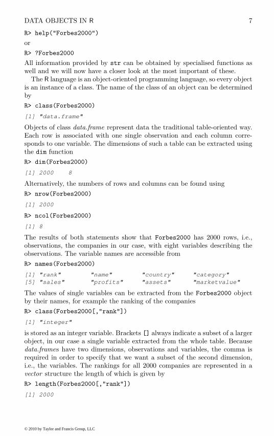
R> help("Forbes2000")
or
R> ?Forbes2000
All information provided by str can be obtained by specialised functions aswell and we will now have a closer look at the most important of these.
The R language is an object-oriented programming language, so every objectis an instance of a class. The name of the class of an object can be determinedby
R> class(Forbes2000)
[1] "data.frame"
Objects of class data.frame represent data the traditional table-oriented way.Each row is associated with one single observation and each column corre-sponds to one variable. The dimensions of such a table can be extracted usingthe dim function
R> dim(Forbes2000)
[1] 2000 8
Alternatively, the numbers of rows and columns can be found using
R> nrow(Forbes2000)
[1] 2000
R> ncol(Forbes2000)
[1] 8
The results of both statements show that Forbes2000 has 2000 rows, i.e.,observations, the companies in our case, with eight variables describing theobservations. The variable names are accessible from
R> names(Forbes2000)
[1] "rank" "name" "country" "category"
[5] "sales" "profits" "assets" "marketvalue"
The values of single variables can be extracted from the Forbes2000 objectby their names, for example the ranking of the companies
R> class(Forbes2000[,"rank"])
[1] "integer"
is stored as an integer variable. Brackets [] always indicate a subset of a largerobject, in our case a single variable extracted from the whole table. Becausedata.frames have two dimensions, observations and variables, the comma isrequired in order to specify that we want a subset of the second dimension,i.e., the variables. The rankings for all 2000 companies are represented in avector structure the length of which is given by
R> length(Forbes2000[,"rank"])
[1] 2000
© 2010 by Taylor and Francis Group, LLC

8 AN INTRODUCTION TO R
A vector is the elementary structure for data handling in R and is a set ofsimple elements, all being objects of the same class. For example, a simplevector of the numbers one to three can be constructed by one of the followingcommands
R> 1:3
[1] 1 2 3
R> c(1,2,3)
[1] 1 2 3
R> seq(from = 1, to = 3, by = 1)
[1] 1 2 3
The unique names of all 2000 companies are stored in a character vector
R> class(Forbes2000[,"name"])
[1] "character"
R> length(Forbes2000[,"name"])
[1] 2000
and the first element of this vector is
R> Forbes2000[,"name"][1]
[1] "Citigroup"
Because the companies are ranked, Citigroup is the world’s largest companyaccording to the Forbes 2000 list. Further details on vectors and subsettingare given in Section 1.6.
Nominal measurements are represented by factor variables in R, such as thecategory of the company’s business segment
R> class(Forbes2000[,"category"])
[1] "factor"
Objects of class factor and character basically differ in the way their valuesare stored internally. Each element of a vector of class character is stored as acharacter variable whereas an integer variable indicating the level of a factoris saved for factor objects. In our case, there are
R> nlevels(Forbes2000[,"category"])
[1] 27
different levels, i.e., business categories, which can be extracted by
R> levels(Forbes2000[,"category"])
[1] "Aerospace & defense"
[2] "Banking"
[3] "Business services & supplies"
...
© 2010 by Taylor and Francis Group, LLC

DATA IMPORT AND EXPORT 9
As a simple summary statistic, the frequencies of the levels of such a factorvariable can be found from
R> table(Forbes2000[,"category"])
Aerospace & defense Banking
19 313
Business services & supplies
70
...
The sales, assets, profits and market value variables are of type numeric,the natural data type for continuous or discrete measurements, for example
R> class(Forbes2000[,"sales"])
[1] "numeric"
and simple summary statistics such as the mean, median and range can befound from
R> median(Forbes2000[,"sales"])
[1] 4.365
R> mean(Forbes2000[,"sales"])
[1] 9.69701
R> range(Forbes2000[,"sales"])
[1] 0.01 256.33
The summary method can be applied to a numeric vector to give a set of usefulsummary statistics, namely the minimum, maximum, mean, median and the25% and 75% quartiles; for example
R> summary(Forbes2000[,"sales"])
Min. 1st Qu. Median Mean 3rd Qu. Max.
0.010 2.018 4.365 9.697 9.548 256.300
1.5 Data Import and Export
In the previous section, the data from the Forbes 2000 list of the world’s largestcompanies were loaded into R from the HSAUR2 package but we will now ex-plore practically more relevant ways to import data into the R system. Themost frequent data formats the data analyst is confronted with are comma sep-arated files, Excel spreadsheets, files in SPSS format and a variety of SQL database engines. Querying data bases is a nontrivial task and requires additionalknowledge about querying languages, and we therefore refer to the R DataImport/Export manual – see Section 1.3. We assume that a comma separatedfile containing the Forbes 2000 list is available as Forbes2000.csv (such a fileis part of the HSAUR2 source package in directory HSAUR2/inst/rawdata).When the fields are separated by commas and each row begins with a name(a text format typically created by Excel), we can read in the data as followsusing the read.table function
© 2010 by Taylor and Francis Group, LLC
10 AN INTRODUCTION TO R
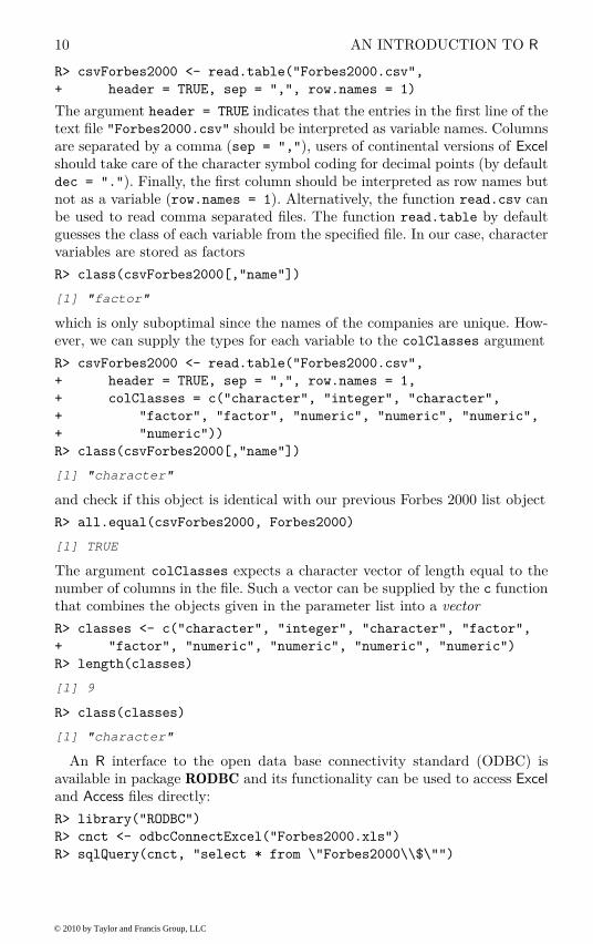
R> csvForbes2000 <- read.table("Forbes2000.csv",
+ header = TRUE, sep = ",", row.names = 1)
The argument header = TRUE indicates that the entries in the first line of thetext file "Forbes2000.csv" should be interpreted as variable names. Columnsare separated by a comma (sep = ","), users of continental versions of Excel
should take care of the character symbol coding for decimal points (by defaultdec = "."). Finally, the first column should be interpreted as row names butnot as a variable (row.names = 1). Alternatively, the function read.csv canbe used to read comma separated files. The function read.table by defaultguesses the class of each variable from the specified file. In our case, charactervariables are stored as factors
R> class(csvForbes2000[,"name"])
[1] "factor"
which is only suboptimal since the names of the companies are unique. How-ever, we can supply the types for each variable to the colClasses argument
R> csvForbes2000 <- read.table("Forbes2000.csv",
+ header = TRUE, sep = ",", row.names = 1,
+ colClasses = c("character", "integer", "character",
+ "factor", "factor", "numeric", "numeric", "numeric",
+ "numeric"))
R> class(csvForbes2000[,"name"])
[1] "character"
and check if this object is identical with our previous Forbes 2000 list object
R> all.equal(csvForbes2000, Forbes2000)
[1] TRUE
The argument colClasses expects a character vector of length equal to thenumber of columns in the file. Such a vector can be supplied by the c functionthat combines the objects given in the parameter list into a vector
R> classes <- c("character", "integer", "character", "factor",
+ "factor", "numeric", "numeric", "numeric", "numeric")
R> length(classes)
[1] 9
R> class(classes)
[1] "character"
An R interface to the open data base connectivity standard (ODBC) isavailable in package RODBC and its functionality can be used to access Excel
and Access files directly:
R> library("RODBC")
R> cnct <- odbcConnectExcel("Forbes2000.xls")
R> sqlQuery(cnct, "select * from \"Forbes2000\\$\"")
© 2010 by Taylor and Francis Group, LLC
BASIC DATA MANIPULATION 11
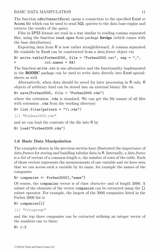
The function odbcConnectExcel opens a connection to the specified Excel orAccess file which can be used to send SQL queries to the data base engine andretrieve the results of the query.
Files in SPSS format are read in a way similar to reading comma separatedfiles, using the function read.spss from package foreign (which comes withthe base distribution).
Exporting data from R is now rather straightforward. A comma separatedfile readable by Excel can be constructed from a data.frame object via
R> write.table(Forbes2000, file = "Forbes2000.csv", sep = ",",
+ col.names = NA)
The function write.csv is one alternative and the functionality implementedin the RODBC package can be used to write data directly into Excel spread-sheets as well.
Alternatively, when data should be saved for later processing in R only, R
objects of arbitrary kind can be stored into an external binary file via
R> save(Forbes2000, file = "Forbes2000.rda")
where the extension .rda is standard. We can get the file names of all fileswith extension .rda from the working directory
R> list.files(pattern = "\\.rda")
[1] "Forbes2000.rda"
and we can load the contents of the file into R by
R> load("Forbes2000.rda")
1.6 Basic Data Manipulation
The examples shown in the previous section have illustrated the importance ofdata.frames for storing and handling tabular data in R. Internally, a data.frameis a list of vectors of a common length n, the number of rows of the table. Eachof those vectors represents the measurements of one variable and we have seenthat we can access such a variable by its name, for example the names of thecompanies
R> companies <- Forbes2000[,"name"]
Of course, the companies vector is of class character and of length 2000. Asubset of the elements of the vector companies can be extracted using the []
subset operator. For example, the largest of the 2000 companies listed in theForbes 2000 list is
R> companies[1]
[1] "Citigroup"
and the top three companies can be extracted utilising an integer vector ofthe numbers one to three:
R> 1:3
© 2010 by Taylor and Francis Group, LLC
12 AN INTRODUCTION TO R
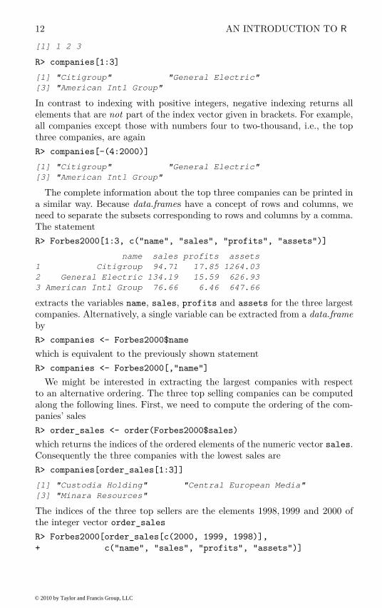
[1] 1 2 3
R> companies[1:3]
[1] "Citigroup" "General Electric"
[3] "American Intl Group"
In contrast to indexing with positive integers, negative indexing returns allelements that are not part of the index vector given in brackets. For example,all companies except those with numbers four to two-thousand, i.e., the topthree companies, are again
R> companies[-(4:2000)]
[1] "Citigroup" "General Electric"
[3] "American Intl Group"
The complete information about the top three companies can be printed ina similar way. Because data.frames have a concept of rows and columns, weneed to separate the subsets corresponding to rows and columns by a comma.The statement
R> Forbes2000[1:3, c("name", "sales", "profits", "assets")]
name sales profits assets
1 Citigroup 94.71 17.85 1264.03
2 General Electric 134.19 15.59 626.93
3 American Intl Group 76.66 6.46 647.66
extracts the variables name, sales, profits and assets for the three largestcompanies. Alternatively, a single variable can be extracted from a data.frameby
R> companies <- Forbes2000$name
which is equivalent to the previously shown statement
R> companies <- Forbes2000[,"name"]
We might be interested in extracting the largest companies with respectto an alternative ordering. The three top selling companies can be computedalong the following lines. First, we need to compute the ordering of the com-panies’ sales
R> order_sales <- order(Forbes2000$sales)
which returns the indices of the ordered elements of the numeric vector sales.Consequently the three companies with the lowest sales are
R> companies[order_sales[1:3]]
[1] "Custodia Holding" "Central European Media"
[3] "Minara Resources"
The indices of the three top sellers are the elements 1998, 1999 and 2000 ofthe integer vector order_sales
R> Forbes2000[order_sales[c(2000, 1999, 1998)],
+ c("name", "sales", "profits", "assets")]
© 2010 by Taylor and Francis Group, LLC
BASIC DATA MANIPULATION 13
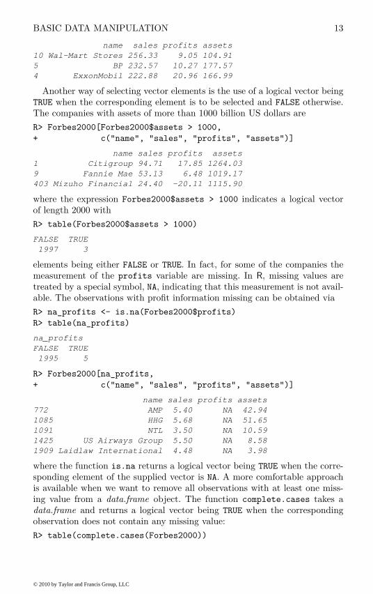
name sales profits assets
10 Wal-Mart Stores 256.33 9.05 104.91
5 BP 232.57 10.27 177.57
4 ExxonMobil 222.88 20.96 166.99
Another way of selecting vector elements is the use of a logical vector beingTRUE when the corresponding element is to be selected and FALSE otherwise.The companies with assets of more than 1000 billion US dollars are
R> Forbes2000[Forbes2000$assets > 1000,
+ c("name", "sales", "profits", "assets")]
name sales profits assets
1 Citigroup 94.71 17.85 1264.03
9 Fannie Mae 53.13 6.48 1019.17
403 Mizuho Financial 24.40 -20.11 1115.90
where the expression Forbes2000$assets > 1000 indicates a logical vectorof length 2000 with
R> table(Forbes2000$assets > 1000)
FALSE TRUE
1997 3
elements being either FALSE or TRUE. In fact, for some of the companies themeasurement of the profits variable are missing. In R, missing values aretreated by a special symbol, NA, indicating that this measurement is not avail-able. The observations with profit information missing can be obtained via
R> na_profits <- is.na(Forbes2000$profits)
R> table(na_profits)
na_profits
FALSE TRUE
1995 5
R> Forbes2000[na_profits,
+ c("name", "sales", "profits", "assets")]
name sales profits assets
772 AMP 5.40 NA 42.94
1085 HHG 5.68 NA 51.65
1091 NTL 3.50 NA 10.59
1425 US Airways Group 5.50 NA 8.58
1909 Laidlaw International 4.48 NA 3.98
where the function is.na returns a logical vector being TRUE when the corre-sponding element of the supplied vector is NA. A more comfortable approachis available when we want to remove all observations with at least one miss-ing value from a data.frame object. The function complete.cases takes adata.frame and returns a logical vector being TRUE when the correspondingobservation does not contain any missing value:
R> table(complete.cases(Forbes2000))
© 2010 by Taylor and Francis Group, LLC

14 AN INTRODUCTION TO R
FALSE TRUE
5 1995
Subsetting data.frames driven by logical expressions may induce a lot oftyping which can be avoided. The subset function takes a data.frame as firstargument and a logical expression as second argument. For example, we canselect a subset of the Forbes 2000 list consisting of all companies situated inthe United Kingdom by
R> UKcomp <- subset(Forbes2000, country == "United Kingdom")
R> dim(UKcomp)
[1] 137 8
i.e., 137 of the 2000 companies are from the UK. Note that it is not neces-sary to extract the variable country from the data.frame Forbes2000 whenformulating the logical expression with subset.
1.7 Computing with Data
1.7.1 Simple Summary Statistics
Two functions are helpful for getting an overview about R objects: str andsummary, where str is more detailed about data types and summary gives acollection of sensible summary statistics. For example, applying the summary
method to the Forbes2000 data set,
R> summary(Forbes2000)
results in the following output
rank name country
Min. : 1.0 Length:2000 United States :751
1st Qu.: 500.8 Class :character Japan :316
Median :1000.5 Mode :character United Kingdom:137
Mean :1000.5 Germany : 65
3rd Qu.:1500.2 France : 63
Max. :2000.0 Canada : 56
(Other) :612
category sales
Banking : 313 Min. : 0.010
Diversified financials: 158 1st Qu.: 2.018
Insurance : 112 Median : 4.365
Utilities : 110 Mean : 9.697
Materials : 97 3rd Qu.: 9.547
Oil & gas operations : 90 Max. :256.330
(Other) :1120
profits assets marketvalue
Min. :-25.8300 Min. : 0.270 Min. : 0.02
1st Qu.: 0.0800 1st Qu.: 4.025 1st Qu.: 2.72
Median : 0.2000 Median : 9.345 Median : 5.15
Mean : 0.3811 Mean : 34.042 Mean : 11.88
3rd Qu.: 0.4400 3rd Qu.: 22.793 3rd Qu.: 10.60
© 2010 by Taylor and Francis Group, LLC

COMPUTING WITH DATA 15
Max. : 20.9600 Max. :1264.030 Max. :328.54
NA's : 5.0000
From this output we can immediately see that most of the companies aresituated in the US and that most of the companies are working in the bankingsector as well as that negative profits, or losses, up to 26 billion US dollarsoccur.
Internally, summary is a so-called generic function with methods for a multi-tude of classes, i.e., summary can be applied to objects of different classes andwill report sensible results. Here, we supply a data.frame object to summary
where it is natural to apply summary to each of the variables in this data.frame.Because a data.frame is a list with each variable being an element of that list,the same effect can be achieved by
R> lapply(Forbes2000, summary)
The members of the apply family help to solve recurring tasks for eachelement of a data.frame, matrix, list or for each level of a factor. It might beinteresting to compare the profits in each of the 27 categories. To do so, wefirst compute the median profit for each category from
R> mprofits <- tapply(Forbes2000$profits,
+ Forbes2000$category, median, na.rm = TRUE)
a command that should be read as follows. For each level of the factor cat-
egory, determine the corresponding elements of the numeric vector profits
and supply them to the median function with additional argument na.rm =
TRUE. The latter one is necessary because profits contains missing valueswhich would lead to a non-sensible result of the median function
R> median(Forbes2000$profits)
[1] NA
The three categories with highest median profit are computed from the vectorof sorted median profits
R> rev(sort(mprofits))[1:3]
Oil & gas operations Drugs & biotechnology
0.35 0.35
Household & personal products
0.31
where rev rearranges the vector of median profits sorted from smallest tolargest. Of course, we can replace the median function with mean or whateveris appropriate in the call to tapply. In our situation, mean is not a good choice,because the distributions of profits or sales are naturally skewed. Simple graph-ical tools for the inspection of the empirical distributions are introduced lateron and in Chapter 2.
1.7.2 Customising Analyses
In the preceding sections we have done quite complex analyses on our datausing functions available from R. However, the real power of the system comes
© 2010 by Taylor and Francis Group, LLC

16 AN INTRODUCTION TO R
to light when writing our own functions for our own analysis tasks. AlthoughR is a full-featured programming language, writing small helper functions forour daily work is not too complicated. We’ll study two example cases.
At first, we want to add a robust measure of variability to the locationmeasures computed in the previous subsection. In addition to the medianprofit, computed via
R> median(Forbes2000$profits, na.rm = TRUE)
[1] 0.2
we want to compute the inter-quartile range, i.e., the difference betweenthe 3rd and 1st quartile. Although a quick search in the manual pages (viahelp("interquartile")) brings function IQR to our attention, we will ap-proach this task without making use of this tool, but using function quantile
for computing sample quantiles only.A function in R is nothing but an object, and all objects are created equal.
Thus, we ‘just’ have to assign a function object to a variable. A functionobject consists of an argument list, defining arguments and possibly defaultvalues, and a body defining the computations. The body starts and ends withbraces. Of course, the body is assumed to be valid R code. In most cases weexpect a function to return an object, therefore, the body will contain one ormore return statements the arguments of which define the return values.
Returning to our example, we’ll name our function iqr. The iqr functionshould operate on numeric vectors, therefore it should have an argument x.This numeric vector will be passed on to the quantile function for computingthe sample quartiles. The required difference between the 3rd and 1st quartilecan then be computed using diff. The definition of our function reads asfollows
R> iqr <- function(x) {
+ q <- quantile(x, prob = c(0.25, 0.75), names = FALSE)
+ return(diff(q))
+ }
A simple test on simulated data from a standard normal distribution showsthat our first function actually works, a comparison with the IQR functionshows that the result is correct:
R> xdata <- rnorm(100)
R> iqr(xdata)
[1] 1.495980
R> IQR(xdata)
[1] 1.495980
However, when the numeric vector contains missing values, our function failsas the following example shows:
R> xdata[1] <- NA
R> iqr(xdata)
© 2010 by Taylor and Francis Group, LLC

COMPUTING WITH DATA 17
Error in quantile.default(x, prob = c(0.25, 0.75)):
missing values and NaN's not allowed if 'na.rm' is FALSE
In order to make our little function more flexible it would be helpful toadd all arguments of quantile to the argument list of iqr. The copy-and-paste approach that first comes to mind is likely to lead to inconsistenciesand errors, for example when the argument list of quantile changes. Instead,the dot argument, a wildcard for any argument, is more appropriate and weredefine our function accordingly:
R> iqr <- function(x, ...) {
+ q <- quantile(x, prob = c(0.25, 0.75), names = FALSE,
+ ...)
+ return(diff(q))
+ }
R> iqr(xdata, na.rm = TRUE)
[1] 1.503438
R> IQR(xdata, na.rm = TRUE)
[1] 1.503438
Now, we can assess the variability of the profits using our new iqr tool:
R> iqr(Forbes2000$profits, na.rm = TRUE)
[1] 0.36
Since there is no difference between functions that have been written by one ofthe R developers and user-created functions, we can compute the inter-quartilerange of profits for each of the business categories by using our iqr functioninside a tapply statement;
R> iqr_profits <- tapply(Forbes2000$profits,
+ Forbes2000$category, iqr, na.rm = TRUE)
and extract the categories with the smallest and greatest variability
R> levels(Forbes2000$category)[which.min(iqr_profits)]
[1] "Hotels restaurants & leisure"
R> levels(Forbes2000$category)[which.max(iqr_profits)]
[1] "Drugs & biotechnology"
We observe less variable profits in tourism enterprises compared with profitsin the pharmaceutical industry.
As other members of the apply family, tapply is very helpful when the sametask is to be done more than one time. Moreover, its use is more convenientcompared to the usage of for loops. For the sake of completeness, we willcompute the category-wise inter-quartile range of the profits using a for loop.
Like a function, a for loop consists of a body, i.e., a chain of R commandsto be executed. In addition, we need a set of values and a variable that iteratesover this set. Here, the set we are interested in is the business categories:
© 2010 by Taylor and Francis Group, LLC

18 AN INTRODUCTION TO R
R> bcat <- Forbes2000$category
R> iqr_profits2 <- numeric(nlevels(bcat))
R> names(iqr_profits2) <- levels(bcat)
R> for (cat in levels(bcat)) {
+ catprofit <- subset(Forbes2000, category == cat)$profit
+ this_iqr <- iqr(catprofit, na.rm = TRUE)
+ iqr_profits2[levels(bcat) == cat] <- this_iqr
+ }
Compared to the usage of tapply, the above code is rather complicated. Atfirst, we have to set up a vector for storing the results and assign the appro-priate names to it. Next, inside the body of the for loop, the iqr function hasto be called on the appropriate subset of all companies of the current businesscategory cat. The corresponding inter-quartile range must then be assignedto the correct vector element in the result vector. Luckily, such complicatedconstructs will be used in only one of the remaining chapters of the book andare almost always avoidable in practical data analyses.
1.7.3 Simple Graphics
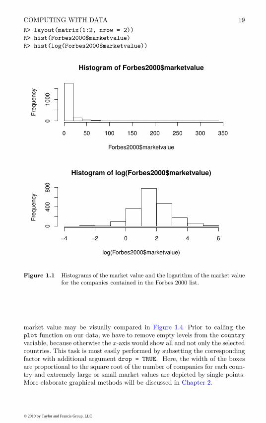
The degree of skewness of a distribution can be investigated by constructinghistograms using the hist function. (More sophisticated alternatives such assmooth density estimates will be considered in Chapter 8.) For example, thecode for producing Figure 1.1 first divides the plot region into two equallyspaced rows (the layout function) and then plots the histograms of the rawmarket values in the upper part using the hist function. The lower part ofthe figure depicts the histogram for the log transformed market values whichappear to be more symmetric.
Bivariate relationships of two continuous variables are usually depicted asscatterplots. In R, regression relationships are specified by so-called modelformulae which, in a simple bivariate case, may look like
R> fm <- marketvalue ~ sales
R> class(fm)
[1] "formula"
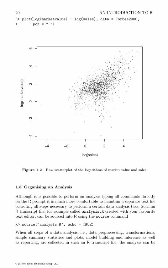
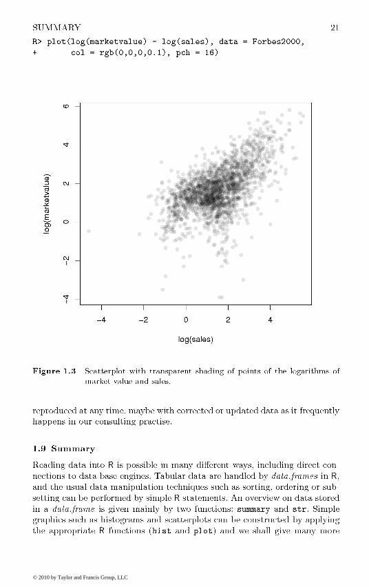
with the dependent variable on the left hand side and the independent variableon the right hand side. The tilde separates left and right hand sides. Such amodel formula can be passed to a model function (for example to the linearmodel function as explained in Chapter 6). The plot generic function imple-ments a formula method as well. Because the distributions of both marketvalue and sales are skewed we choose to depict their logarithms. A raw scat-terplot of 2000 data points (Figure 1.2) is rather uninformative due to areaswith very high density. This problem can be avoided by choosing a transparentcolor for the dots as shown in Figure 1.3.
If the independent variable is a factor, a boxplot representation is a naturalchoice. For four selected countries, the distributions of the logarithms of the
© 2010 by Taylor and Francis Group, LLC
COMPUTING WITH DATA 19
R> layout(matrix(1:2, nrow = 2))
R> hist(Forbes2000$marketvalue)
R> hist(log(Forbes2000$marketvalue))
Histogram of Forbes2000$marketvalue
Forbes2000$marketvalue
Fre
qu
en
cy
0 50 100 150 200 250 300 350
01
00
0
Histogram of log(Forbes2000$marketvalue)
log(Forbes2000$marketvalue)
Fre
qu
en
cy
−4 −2 0 2 4 6
04
00
80
0
Figure 1.1 Histograms of the market value and the logarithm of the market value
for the companies contained in the Forbes 2000 list.
market value may be visually compared in Figure 1.4. Prior to calling theplot function on our data, we have to remove empty levels from the country
variable, because otherwise the x-axis would show all and not only the selectedcountries. This task is most easily performed by subsetting the correspondingfactor with additional argument drop = TRUE. Here, the width of the boxesare proportional to the square root of the number of companies for each coun-try and extremely large or small market values are depicted by single points.More elaborate graphical methods will be discussed in Chapter 2.
© 2010 by Taylor and Francis Group, LLC
20 AN INTRODUCTION TO R
R> plot(log(marketvalue) ~ log(sales), data = Forbes2000,
+ pch = ".")
−4 −2 0 2 4
−4
−2
02
46
log(sales)
log
(ma
rke
tva
lue
)
Figure 1.2 Raw scatterplot of the logarithms of market value and sales.
1.8 Organising an Analysis
Although it is possible to perform an analysis typing all commands directlyon the R prompt it is much more comfortable to maintain a separate text filecollecting all steps necessary to perform a certain data analysis task. Such anR transcript file, for example called analysis.R created with your favouritetext editor, can be sourced into R using the source command
R> source("analysis.R", echo = TRUE)
When all steps of a data analysis, i.e., data preprocessing, transformations,simple summary statistics and plots, model building and inference as wellas reporting, are collected in such an R transcript file, the analysis can be
© 2010 by Taylor and Francis Group, LLC
© 2010 by Taylor and Francis Group, LLC

22 AN INTRODUCTION TO R
R> tmp <- subset(Forbes2000,
+ country %in% c("United Kingdom", "Germany",
+ "India", "Turkey"))
R> tmp$country <- tmp$country[,drop = TRUE]
R> plot(log(marketvalue) ~ country, data = tmp,
+ ylab = "log(marketvalue)", varwidth = TRUE)
Germany India Turkey United Kingdom
−2
02
4
country
log
(ma
rke
tva
lue
)
Figure 1.4 Boxplots of the logarithms of the market value for four selected coun-
tries, the width of the boxes is proportional to the square roots of the
number of companies.
© 2010 by Taylor and Francis Group, LLC

SUMMARY 23
examples of these functions and those that produce more interesting graphicsin later chapters.
Exercises
Ex. 1.1 Calculate the median profit for the companies in the US and themedian profit for the companies in the UK, France and Germany.
Ex. 1.2 Find all German companies with negative profit.
Ex. 1.3 To which business category do most of the Bermuda island companiesbelong?
Ex. 1.4 For the 50 companies in the Forbes data set with the highest profits,plot sales against assets (or some suitable transformation of each variable),labelling each point with the appropriate country name which may needto be abbreviated (using abbreviate) to avoid making the plot look too‘messy’.
Ex. 1.5 Find the average value of sales for the companies in each countryin the Forbes data set, and find the number of companies in each countrywith profits above 5 billion US dollars.
© 2010 by Taylor and Francis Group, LLC

CHAPTER 2
Data Analysis Using GraphicalDisplays: Malignant Melanoma in the
USA and Chinese Health andFamily Life
2.1 Introduction
Fisher and Belle (1993) report mortality rates due to malignant melanomaof the skin for white males during the period 1950–1969, for each state onthe US mainland. The data are given in Table 2.1 and include the number ofdeaths due to malignant melanoma in the corresponding state, the longitudeand latitude of the geographic centre of each state, and a binary variableindicating contiguity to an ocean, that is, if the state borders one of theoceans. Questions of interest about these data include: how do the mortalityrates compare for ocean and non-ocean states? and how are mortality ratesaffected by latitude and longitude?
Table 2.1: USmelanoma data. USA mortality rates for whitemales due to malignant melanoma.
mortality latitude longitude ocean
Alabama 219 33.0 87.0 yesArizona 160 34.5 112.0 noArkansas 170 35.0 92.5 noCalifornia 182 37.5 119.5 yesColorado 149 39.0 105.5 noConnecticut 159 41.8 72.8 yesDelaware 200 39.0 75.5 yesDistrict of Columbia 177 39.0 77.0 noFlorida 197 28.0 82.0 yesGeorgia 214 33.0 83.5 yesIdaho 116 44.5 114.0 noIllinois 124 40.0 89.5 noIndiana 128 40.2 86.2 noIowa 128 42.2 93.8 noKansas 166 38.5 98.5 noKentucky 147 37.8 85.0 noLouisiana 190 31.2 91.8 yes
25
© 2010 by Taylor and Francis Group, LLC
26 DATA ANALYSIS USING GRAPHICAL DISPLAYS
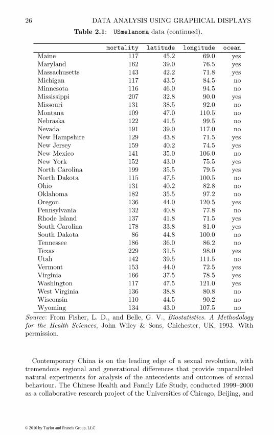
Table 2.1: USmelanoma data (continued).
mortality latitude longitude ocean
Maine 117 45.2 69.0 yesMaryland 162 39.0 76.5 yesMassachusetts 143 42.2 71.8 yesMichigan 117 43.5 84.5 noMinnesota 116 46.0 94.5 noMississippi 207 32.8 90.0 yesMissouri 131 38.5 92.0 noMontana 109 47.0 110.5 noNebraska 122 41.5 99.5 noNevada 191 39.0 117.0 noNew Hampshire 129 43.8 71.5 yesNew Jersey 159 40.2 74.5 yesNew Mexico 141 35.0 106.0 noNew York 152 43.0 75.5 yesNorth Carolina 199 35.5 79.5 yesNorth Dakota 115 47.5 100.5 noOhio 131 40.2 82.8 noOklahoma 182 35.5 97.2 noOregon 136 44.0 120.5 yesPennsylvania 132 40.8 77.8 noRhode Island 137 41.8 71.5 yesSouth Carolina 178 33.8 81.0 yesSouth Dakota 86 44.8 100.0 noTennessee 186 36.0 86.2 noTexas 229 31.5 98.0 yesUtah 142 39.5 111.5 noVermont 153 44.0 72.5 yesVirginia 166 37.5 78.5 yesWashington 117 47.5 121.0 yesWest Virginia 136 38.8 80.8 noWisconsin 110 44.5 90.2 noWyoming 134 43.0 107.5 no
Source: From Fisher, L. D., and Belle, G. V., Biostatistics. A Methodology
for the Health Sciences, John Wiley & Sons, Chichester, UK, 1993. Withpermission.
Contemporary China is on the leading edge of a sexual revolution, withtremendous regional and generational differences that provide unparallelednatural experiments for analysis of the antecedents and outcomes of sexualbehaviour. The Chinese Health and Family Life Study, conducted 1999–2000as a collaborative research project of the Universities of Chicago, Beijing, and
© 2010 by Taylor and Francis Group, LLC
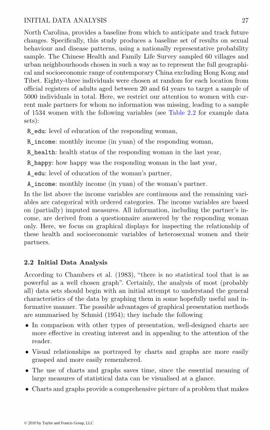
INITIAL DATA ANALYSIS 27
North Carolina, provides a baseline from which to anticipate and track futurechanges. Specifically, this study produces a baseline set of results on sexualbehaviour and disease patterns, using a nationally representative probabilitysample. The Chinese Health and Family Life Survey sampled 60 villages andurban neighbourhoods chosen in such a way as to represent the full geographi-cal and socioeconomic range of contemporary China excluding Hong Kong andTibet. Eighty-three individuals were chosen at random for each location fromofficial registers of adults aged between 20 and 64 years to target a sample of5000 individuals in total. Here, we restrict our attention to women with cur-rent male partners for whom no information was missing, leading to a sampleof 1534 women with the following variables (see Table 2.2 for example datasets):
R_edu: level of education of the responding woman,
R_income: monthly income (in yuan) of the responding woman,
R_health: health status of the responding woman in the last year,
R_happy: how happy was the responding woman in the last year,
A_edu: level of education of the woman’s partner,
A_income: monthly income (in yuan) of the woman’s partner.
In the list above the income variables are continuous and the remaining vari-ables are categorical with ordered categories. The income variables are basedon (partially) imputed measures. All information, including the partner’s in-come, are derived from a questionnaire answered by the responding womanonly. Here, we focus on graphical displays for inspecting the relationship ofthese health and socioeconomic variables of heterosexual women and theirpartners.
2.2 Initial Data Analysis
According to Chambers et al. (1983), “there is no statistical tool that is aspowerful as a well chosen graph”. Certainly, the analysis of most (probablyall) data sets should begin with an initial attempt to understand the generalcharacteristics of the data by graphing them in some hopefully useful and in-formative manner. The possible advantages of graphical presentation methodsare summarised by Schmid (1954); they include the following
• In comparison with other types of presentation, well-designed charts aremore effective in creating interest and in appealing to the attention of thereader.
• Visual relationships as portrayed by charts and graphs are more easilygrasped and more easily remembered.
• The use of charts and graphs saves time, since the essential meaning oflarge measures of statistical data can be visualised at a glance.
• Charts and graphs provide a comprehensive picture of a problem that makes
© 2010 by Taylor and Francis Group, LLC
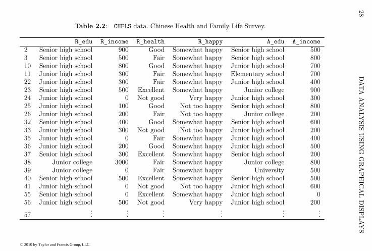
28
DA
TA
AN
ALY
SIS
USIN
GG
RA
PH
ICA
LD
ISP
LA
YS
Table 2.2: CHFLS data. Chinese Health and Family Life Survey.
R_edu R_income R_health R_happy A_edu A_income
2 Senior high school 900 Good Somewhat happy Senior high school 5003 Senior high school 500 Fair Somewhat happy Senior high school 80010 Senior high school 800 Good Somewhat happy Junior high school 70011 Junior high school 300 Fair Somewhat happy Elementary school 70022 Junior high school 300 Fair Somewhat happy Junior high school 40023 Senior high school 500 Excellent Somewhat happy Junior college 90024 Junior high school 0 Not good Very happy Junior high school 30025 Junior high school 100 Good Not too happy Senior high school 80026 Junior high school 200 Fair Not too happy Junior college 20032 Senior high school 400 Good Somewhat happy Senior high school 60033 Junior high school 300 Not good Not too happy Junior high school 20035 Junior high school 0 Fair Somewhat happy Junior high school 40036 Junior high school 200 Good Somewhat happy Junior high school 50037 Senior high school 300 Excellent Somewhat happy Senior high school 20038 Junior college 3000 Fair Somewhat happy Junior college 80039 Junior college 0 Fair Somewhat happy University 50040 Senior high school 500 Excellent Somewhat happy Senior high school 50041 Junior high school 0 Not good Not too happy Junior high school 60055 Senior high school 0 Excellent Somewhat happy Junior high school 056 Junior high school 500 Not good Very happy Junior high school 200
57...
......
......
...
© 2010 by Taylor and Francis Group, LLC

ANALYSIS USING R 29
for a more complete and better balanced understanding than could be de-rived from tabular or textual forms of presentation.
• Charts and graphs can bring out hidden facts and relationships and canstimulate, as well as aid, analytical thinking and investigation.
Graphs are very popular; it has been estimated that between 900 billion (9 ×
1011) and 2 trillion (2 × 10¹²) images of statistical graphics are printed eachyear. Perhaps one of the main reasons for such popularity is that graphicalpresentation of data often provides the vehicle for discovering the unexpected;the human visual system is very powerful in detecting patterns, although thefollowing caveat from the late Carl Sagan (in his book Contact) should bekept in mind:
Humans are good at discerning subtle patterns that are really there, but equallyso at imagining them when they are altogether absent.
During the last two decades a wide variety of new methods for displaying datagraphically have been developed; these will hunt for special effects in data,indicate outliers, identify patterns, diagnose models and generally search fornovel and perhaps unexpected phenomena. Large numbers of graphs may berequired and computers are generally needed to supply them for the samereasons they are used for numerical analyses, namely that they are fast andthey are accurate.
So, because the machine is doing the work the question is no longer“shall weplot?” but rather “what shall we plot?” There are many exciting possibilitiesincluding dynamic graphics but graphical exploration of data usually begins,at least, with some simpler, well-known methods, for example, histograms,barcharts, boxplots and scatterplots. Each of these will be illustrated in thischapter along with more complex methods such as spinograms and trellis plots.
2.3 Analysis Using R
2.3.1 Malignant Melanoma
We might begin to examine the malignant melanoma data in Table 2.1 by con-structing a histogram or boxplot for all the mortality rates in Figure 2.1. Theplot, hist and boxplot functions have already been introduced in Chapter 1and we want to produce a plot where both techniques are applied at once.The layout function organises two independent plots on one plotting device,for example on top of each other. Using this relatively simple technique (moreadvanced methods will be introduced later) we have to make sure that thex-axis is the same in both graphs. This can be done by computing a plausiblerange of the data, later to be specified in a plot via the xlim argument:
R> xr <- range(USmelanoma$mortality) * c(0.9, 1.1)
R> xr
[1] 77.4 251.9
Now, plotting both the histogram and the boxplot requires setting up theplotting device with equal space for two independent plots on top of each other.
© 2010 by Taylor and Francis Group, LLC
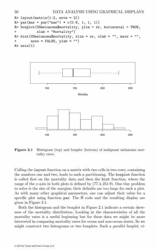
30 DATA ANALYSIS USING GRAPHICAL DISPLAYS
R> layout(matrix(1:2, nrow = 2))
R> par(mar = par("mar") * c(0.8, 1, 1, 1))
R> boxplot(USmelanoma$mortality, ylim = xr, horizontal = TRUE,
+ xlab = "Mortality")
R> hist(USmelanoma$mortality, xlim = xr, xlab = "", main = "",
+ axes = FALSE, ylab = "")
R> axis(1)
100 150 200 250
Mortality
100 150 200 250
Figure 2.1 Histogram (top) and boxplot (bottom) of malignant melanoma mor-tality rates.
Calling the layout function on a matrix with two cells in two rows, containingthe numbers one and two, leads to such a partitioning. The boxplot functionis called first on the mortality data and then the hist function, where therange of the x-axis in both plots is defined by (77.4, 251.9). One tiny problemto solve is the size of the margins; their defaults are too large for such a plot.As with many other graphical parameters, one can adjust their value for aspecific plot using function par. The R code and the resulting display aregiven in Figure 2.1.
Both the histogram and the boxplot in Figure 2.1 indicate a certain skew-ness of the mortality distribution. Looking at the characteristics of all themortality rates is a useful beginning but for these data we might be moreinterested in comparing mortality rates for ocean and non-ocean states. So wemight construct two histograms or two boxplots. Such a parallel boxplot, vi-
© 2010 by Taylor and Francis Group, LLC

ANALYSIS USING R 31
R> plot(mortality ~ ocean, data = USmelanoma,
+ xlab = "Contiguity to an ocean", ylab = "Mortality")
no yes
10
01
20
14
01
60
18
02
00
22
0
Contiguity to an ocean
Mo
rta
lity
Figure 2.2 Parallel boxplots of malignant melanoma mortality rates by contiguityto an ocean.
sualising the conditional distribution of a numeric variable in groups as givenby a categorical variable, are easily computed using the boxplot function.The continuous response variable and the categorical independent variableare specified via a formula as described in Chapter 1. Figure 2.2 shows suchparallel boxplots, as by default produced the plot function for such data, forthe mortality in ocean and non-ocean states and leads to the impression thatthe mortality is increased in east or west coast states compared to the rest ofthe country.
Histograms are generally used for two purposes: counting and displaying thedistribution of a variable; according to Wilkinson (1992), “they are effectivefor neither”. Histograms can often be misleading for displaying distributionsbecause of their dependence on the number of classes chosen. An alternativeis to formally estimate the density function of a variable and then plot theresulting estimate; details of density estimation are given in Chapter 8 but forthe ocean and non-ocean states the two density estimates can be produced andplotted as shown in Figure 2.3 which supports the impression from Figure 2.2.For more details on such density estimates we refer to Chapter 8.
© 2010 by Taylor and Francis Group, LLC

32 DATA ANALYSIS USING GRAPHICAL DISPLAYS
R> dyes <- with(USmelanoma, density(mortality[ocean == "yes"]))
R> dno <- with(USmelanoma, density(mortality[ocean == "no"]))
R> plot(dyes, lty = 1, xlim = xr, main = "", ylim = c(0, 0.018))
R> lines(dno, lty = 2)
R> legend("topleft", lty = 1:2, legend = c("Coastal State",
+ "Land State"), bty = "n")
100 150 200 250
0.0
00
0.0
05
0.0
10
0.0
15
N = 22 Bandwidth = 16.22
De
nsity
Coastal StateLand State
Figure 2.3 Estimated densities of malignant melanoma mortality rates by conti-guity to an ocean.
Now we might move on to look at how mortality rates are related to thegeographic location of a state as represented by the latitude and longitudeof the centre of the state. Here the main graphic will be the scatterplot. Thesimple xy scatterplot has been in use since at least the eighteenth century andhas many virtues – indeed according to Tufte (1983):
The relational graphic – in its barest form the scatterplot and its variants – isthe greatest of all graphical designs. It links at least two variables, encouragingand even imploring the viewer to assess the possible causal relationship betweenthe plotted variables. It confronts causal theories that x causes y with empiricalevidence as to the actual relationship between x and y.
Let’s begin with simple scatterplots of mortality rate against longitude andmortality rate against latitude which can be produced by the code precedingFigure 2.4. Again, the layout function is used for partitioning the plottingdevice, now resulting in two side by-side-plots. The argument to layout is
© 2010 by Taylor and Francis Group, LLC
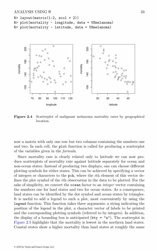
ANALYSIS USING R 33
R> layout(matrix(1:2, ncol = 2))
R> plot(mortality ~ longitude, data = USmelanoma)
R> plot(mortality ~ latitude, data = USmelanoma)
70 80 90 100 110 120
10
01
40
18
02
20
longitude
mo
rta
lity
30 35 40 45
10
01
40
18
02
20
latitude
mo
rta
lity
Figure 2.4 Scatterplot of malignant melanoma mortality rates by geographicallocation.
now a matrix with only one row but two columns containing the numbers oneand two. In each cell, the plot function is called for producing a scatterplotof the variables given in the formula.
Since mortality rate is clearly related only to latitude we can now pro-duce scatterplots of mortality rate against latitude separately for ocean andnon-ocean states. Instead of producing two displays, one can choose differentplotting symbols for either states. This can be achieved by specifying a vectorof integers or characters to the pch, where the ith element of this vector de-fines the plot symbol of the ith observation in the data to be plotted. For thesake of simplicity, we convert the ocean factor to an integer vector containingthe numbers one for land states and two for ocean states. As a consequence,land states can be identified by the dot symbol and ocean states by triangles.It is useful to add a legend to such a plot, most conveniently by using thelegend function. This function takes three arguments: a string indicating theposition of the legend in the plot, a character vector of labels to be printedand the corresponding plotting symbols (referred to by integers). In addition,the display of a bounding box is anticipated (bty = "n"). The scatterplot inFigure 2.5 highlights that the mortality is lowest in the northern land states.Coastal states show a higher mortality than land states at roughly the same
© 2010 by Taylor and Francis Group, LLC

34 DATA ANALYSIS USING GRAPHICAL DISPLAYS
R> plot(mortality ~ latitude, data = USmelanoma,
+ pch = as.integer(USmelanoma$ocean))
R> legend("topright", legend = c("Land state", "Coast state"),
+ pch = 1:2, bty = "n")
30 35 40 45
10
01
20
14
01
60
18
02
00
22
0
latitude
mo
rta
lity
Land stateCoast state
Figure 2.5 Scatterplot of malignant melanoma mortality rates against latitude.
latitude. The highest mortalities can be observed for the south coastal stateswith latitude less than 32◦, say, that is
R> subset(USmelanoma, latitude < 32)
mortality latitude longitude ocean
Florida 197 28.0 82.0 yes
Louisiana 190 31.2 91.8 yes
Texas 229 31.5 98.0 yes
Up to now we have primarily focused on the visualisation of continuousvariables. We now extend our focus to the visualisation of categorical variables.
© 2010 by Taylor and Francis Group, LLC

ANALYSIS USING R 35
R> barplot(xtabs(~ R_happy, data = CHFLS))
Very unhappy Not too happy Somewhat happy Very happy
02
00
40
06
00
80
01
00
0
Figure 2.6 Bar chart of happiness.
2.3.2 Chinese Health and Family Life
One part of the questionnaire the Chinese Health and Family Life Surveyfocuses on is the self-reported health status. Two questions are interesting forus. The first one is “Generally speaking, do you consider the condition of yourhealth to be excellent, good, fair, not good, or poor?”. The second question is“Generally speaking, in the past twelve months, how happy were you?”. Thedistribution of such variables is commonly visualised using barcharts where foreach category the total or relative number of observations is displayed. Sucha barchart can conveniently be produced by applying the barplot functionto a tabulation of the data. The empirical density of the variable R_happy
is computed by the xtabs function for producing (contingency) tables; theresulting barchart is given in Figure 2.6.
The visualisation of two categorical variables could be done by conditionalbarcharts, i.e., barcharts of the first variable within the categories of the sec-ond variable. An attractive alternative for displaying such two-way tables arespineplots (Friendly, 1994, Hofmann and Theus, 2005, Chen et al., 2008);the meaning of the name will become clear when looking at such a plot inFigure 2.7.
Before constructing such a plot, we produce a two-way table of the healthstatus and self-reported happiness using the xtabs function:
© 2010 by Taylor and Francis Group, LLC
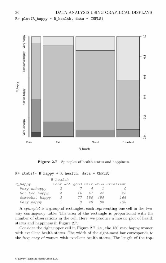
36 DATA ANALYSIS USING GRAPHICAL DISPLAYS
R> plot(R_happy ~ R_health, data = CHFLS)
R_health
R_
ha
ppy
Poor Fair Good Excellent
Ve
ry u
nh
ap
py
No
t to
o h
ap
py
So
mew
ha
t h
ap
py
Ve
ry h
ap
py
0.0
0.2
0.4
0.6
0.8
1.0
Figure 2.7 Spineplot of health status and happiness.
R> xtabs(~ R_happy + R_health, data = CHFLS)
R_health
R_happy Poor Not good Fair Good Excellent
Very unhappy 2 7 4 1 0
Not too happy 4 46 67 42 26
Somewhat happy 3 77 350 459 166
Very happy 1 9 40 80 150
A spineplot is a group of rectangles, each representing one cell in the two-way contingency table. The area of the rectangle is proportional with thenumber of observations in the cell. Here, we produce a mosaic plot of healthstatus and happiness in Figure 2.7.
Consider the right upper cell in Figure 2.7, i.e., the 150 very happy womenwith excellent health status. The width of the right-most bar corresponds tothe frequency of women with excellent health status. The length of the top-
© 2010 by Taylor and Francis Group, LLC

ANALYSIS USING R 37
right rectangle corresponds to the conditional frequency of very happy womengiven their health status is excellent. Multiplying these two quantities givesthe area of this cell which corresponds to the frequency of women who are bothvery happy and enjoy an excellent health status. The conditional frequencyof very happy women increases with increasing health status, whereas theconditional frequency of very unhappy or not too happy women decreases.
When the association of a categorical and a continuous variable is of interest,say the monthly income and self-reported happiness, one might use parallelboxplots to visualise the distribution of the income depending on happiness.If we were studying self-reported happiness as response and income as inde-pendent variable, however, this would give a representation of the conditionaldistribution of income given happiness, but we are interested in the condi-tional distribution of happiness given income. One possibility to produce amore appropriate plot is called spinogram. Here, the continuous x-variable iscategorised first. Within each of these categories, the conditional frequenciesof the response variable are given by stacked barcharts, in a way similar tospineplots. For happiness depending on log-income (since income is naturallyskewed we use a log-transformation of the income) it seems that the propor-tion of unhappy and not too happy women decreases with increasing incomewhereas the proportion of very happy women stays rather constant. In con-trast to spinograms, where bins, as in a histogram, are given on the x-axis, aconditional density plot uses the original x-axis for a display of the conditionaldensity of the categorical response given the independent variable.
For our last example we return to scatterplots for inspecting the associa-tion between a woman’s monthly income and the income of her partner. Bothincome variables have been computed and partially imputed from other self-reported variables and are only rough assessments of the real income. More-over, the data itself is numeric but heavily tied, making it difficult to produce‘correct’ scatterplots because points will overlap. A relatively easy trick is tojitter the observation by adding a small random noise to each point in or-der to avoid overlapping plotting symbols. In addition, we want to study therelationship between both monthly incomes conditional on the woman’s ed-ucation. Such conditioning plots are called trellis plots and are implementedin the package lattice (Sarkar, 2009, 2008). We utilise the xyplot functionfrom package lattice to produce a scatterplot. The formula reads as alreadyexplained with the exception that a third conditioning variable, R_edu in ourcase, is present. For each level of education, a separate scatterplot will be pro-duced. The plots are directly comparable since the axes remain the same forall plots.
The plot reveals several interesting issues. Some observations are positionedon a straight line with slope one, most probably an artifact of missing valueimputation by linear models (as described in the data dictionary, see ?CHFLS).Four constellations can be identified: both partners have zero income, thepartner has no income, the woman has no income or both partners have apositive income.
© 2010 by Taylor and Francis Group, LLC
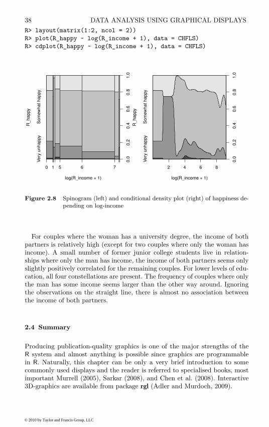
38 DATA ANALYSIS USING GRAPHICAL DISPLAYS
R> layout(matrix(1:2, ncol = 2))
R> plot(R_happy ~ log(R_income + 1), data = CHFLS)
R> cdplot(R_happy ~ log(R_income + 1), data = CHFLS)
log(R_income + 1)
R_
ha
ppy
0 1 5 6 7
Ve
ry u
nh
ap
py
So
mew
ha
t h
ap
py
0.0
0.2
0.4
0.6
0.8
1.0
log(R_income + 1)
R_
ha
ppy
2 4 6 8
Ve
ry u
nh
ap
py
So
mew
ha
t h
ap
py
0.0
0.2
0.4
0.6
0.8
1.0
Figure 2.8 Spinogram (left) and conditional density plot (right) of happiness de-pending on log-income
For couples where the woman has a university degree, the income of bothpartners is relatively high (except for two couples where only the woman hasincome). A small number of former junior college students live in relation-ships where only the man has income, the income of both partners seems onlyslightly positively correlated for the remaining couples. For lower levels of edu-cation, all four constellations are present. The frequency of couples where onlythe man has some income seems larger than the other way around. Ignoringthe observations on the straight line, there is almost no association betweenthe income of both partners.
2.4 Summary
Producing publication-quality graphics is one of the major strengths of theR system and almost anything is possible since graphics are programmablein R. Naturally, this chapter can be only a very brief introduction to somecommonly used displays and the reader is referred to specialised books, mostimportant Murrell (2005), Sarkar (2008), and Chen et al. (2008). Interactive3D-graphics are available from package rgl (Adler and Murdoch, 2009).
© 2010 by Taylor and Francis Group, LLC
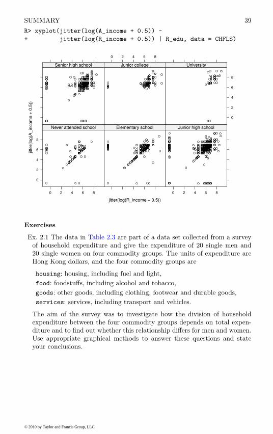
SUMMARY 39
R> xyplot(jitter(log(A_income + 0.5)) ~
+ jitter(log(R_income + 0.5)) | R_edu, data = CHFLS)
jitter(log(R_income + 0.5))
jitte
r(lo
g(A
_in
co
me
+ 0
.5))
0
2
4
6
8
0 2 4 6 8
Never attended school Elementary school
0 2 4 6 8
Junior high school
Senior high school
0 2 4 6 8
Junior college
0
2
4
6
8
University
Exercises
Ex. 2.1 The data in Table 2.3 are part of a data set collected from a surveyof household expenditure and give the expenditure of 20 single men and20 single women on four commodity groups. The units of expenditure areHong Kong dollars, and the four commodity groups are
housing: housing, including fuel and light,
food: foodstuffs, including alcohol and tobacco,
goods: other goods, including clothing, footwear and durable goods,
services: services, including transport and vehicles.
The aim of the survey was to investigate how the division of householdexpenditure between the four commodity groups depends on total expen-diture and to find out whether this relationship differs for men and women.Use appropriate graphical methods to answer these questions and stateyour conclusions.
© 2010 by Taylor and Francis Group, LLC
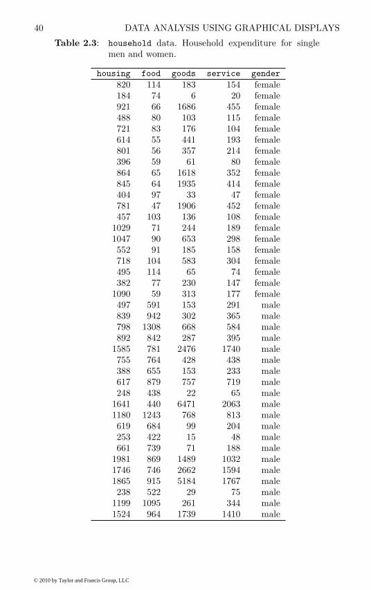
40 DATA ANALYSIS USING GRAPHICAL DISPLAYS
Table 2.3: household data. Household expenditure for singlemen and women.
housing food goods service gender
820 114 183 154 female184 74 6 20 female921 66 1686 455 female488 80 103 115 female721 83 176 104 female614 55 441 193 female801 56 357 214 female396 59 61 80 female864 65 1618 352 female845 64 1935 414 female404 97 33 47 female781 47 1906 452 female457 103 136 108 female
1029 71 244 189 female1047 90 653 298 female552 91 185 158 female718 104 583 304 female495 114 65 74 female382 77 230 147 female
1090 59 313 177 female497 591 153 291 male839 942 302 365 male798 1308 668 584 male892 842 287 395 male
1585 781 2476 1740 male755 764 428 438 male388 655 153 233 male617 879 757 719 male248 438 22 65 male
1641 440 6471 2063 male1180 1243 768 813 male619 684 99 204 male253 422 15 48 male661 739 71 188 male
1981 869 1489 1032 male1746 746 2662 1594 male1865 915 5184 1767 male238 522 29 75 male
1199 1095 261 344 male1524 964 1739 1410 male
© 2010 by Taylor and Francis Group, LLC
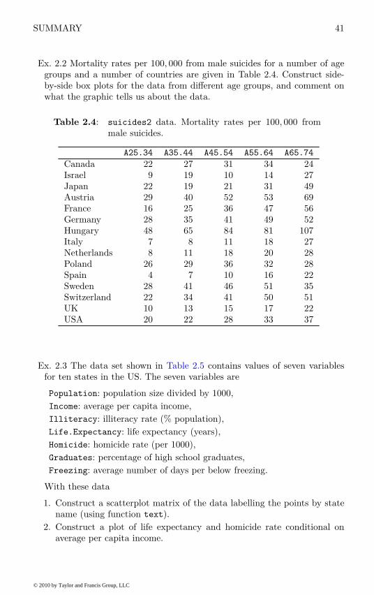
SUMMARY 41
Ex. 2.2 Mortality rates per 100, 000 from male suicides for a number of agegroups and a number of countries are given in Table 2.4. Construct side-by-side box plots for the data from different age groups, and comment onwhat the graphic tells us about the data.
Table 2.4: suicides2 data. Mortality rates per 100, 000 frommale suicides.
A25.34 A35.44 A45.54 A55.64 A65.74
Canada 22 27 31 34 24Israel 9 19 10 14 27Japan 22 19 21 31 49Austria 29 40 52 53 69France 16 25 36 47 56Germany 28 35 41 49 52Hungary 48 65 84 81 107Italy 7 8 11 18 27Netherlands 8 11 18 20 28Poland 26 29 36 32 28Spain 4 7 10 16 22Sweden 28 41 46 51 35Switzerland 22 34 41 50 51UK 10 13 15 17 22USA 20 22 28 33 37
Ex. 2.3 The data set shown in Table 2.5 contains values of seven variablesfor ten states in the US. The seven variables are
Population: population size divided by 1000,
Income: average per capita income,
Illiteracy: illiteracy rate (% population),
Life.Expectancy: life expectancy (years),
Homicide: homicide rate (per 1000),
Graduates: percentage of high school graduates,
Freezing: average number of days per below freezing.
With these data
1. Construct a scatterplot matrix of the data labelling the points by statename (using function text).
2. Construct a plot of life expectancy and homicide rate conditional onaverage per capita income.
© 2010 by Taylor and Francis Group, LLC

42
DA
TA
AN
ALY
SIS
USIN
GG
RA
PH
ICA
LD
ISP
LA
YS
Table 2.5: USstates data. Socio-demographic variables for tenUS states.
Population Income Illiteracy Life.Expectancy Homicide Graduates Freezing
3615 3624 2.1 69.05 15.1 41.3 2021198 5114 1.1 71.71 10.3 62.6 202861 4628 0.5 72.56 2.3 59.0 1402341 3098 2.4 68.09 12.5 41.0 50812 4281 0.7 71.23 3.3 57.6 174
10735 4561 0.8 70.82 7.4 53.2 1242284 4660 0.6 72.13 4.2 60.0 44
11860 4449 1.0 70.43 6.1 50.2 126681 4167 0.5 72.08 1.7 52.3 172472 3907 0.6 71.64 5.5 57.1 168
© 2010 by Taylor and Francis Group, LLC
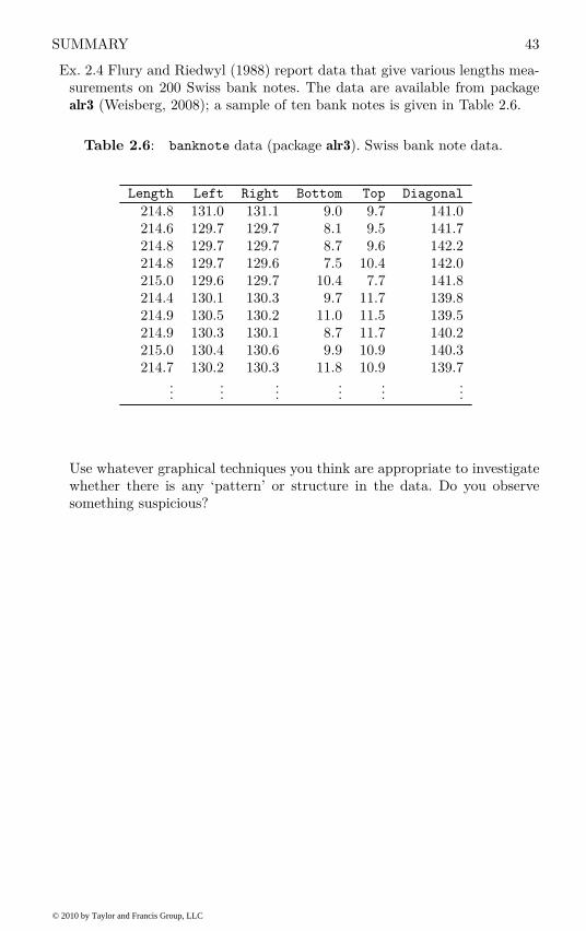
SUMMARY 43
Ex. 2.4 Flury and Riedwyl (1988) report data that give various lengths mea-surements on 200 Swiss bank notes. The data are available from packagealr3 (Weisberg, 2008); a sample of ten bank notes is given in Table 2.6.
Table 2.6: banknote data (package alr3). Swiss bank note data.
Length Left Right Bottom Top Diagonal
214.8 131.0 131.1 9.0 9.7 141.0214.6 129.7 129.7 8.1 9.5 141.7214.8 129.7 129.7 8.7 9.6 142.2214.8 129.7 129.6 7.5 10.4 142.0215.0 129.6 129.7 10.4 7.7 141.8214.4 130.1 130.3 9.7 11.7 139.8214.9 130.5 130.2 11.0 11.5 139.5214.9 130.3 130.1 8.7 11.7 140.2215.0 130.4 130.6 9.9 10.9 140.3214.7 130.2 130.3 11.8 10.9 139.7
......
......
......
Use whatever graphical techniques you think are appropriate to investigatewhether there is any ‘pattern’ or structure in the data. Do you observesomething suspicious?
© 2010 by Taylor and Francis Group, LLC
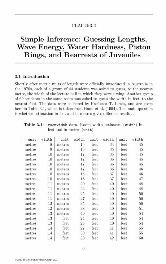
CHAPTER 3
Simple Inference: Guessing Lengths,Wave Energy, Water Hardness, Piston
Rings, and Rearrests of Juveniles
3.1 Introduction
Shortly after metric units of length were officially introduced in Australia inthe 1970s, each of a group of 44 students was asked to guess, to the nearestmetre, the width of the lecture hall in which they were sitting. Another groupof 69 students in the same room was asked to guess the width in feet, to thenearest foot. The data were collected by Professor T. Lewis, and are givenhere in Table 3.1, which is taken from Hand et al. (1994). The main questionis whether estimation in feet and in metres gives different results.
Table 3.1: roomwidth data. Room width estimates (width) infeet and in metres (unit).
unit width unit width unit width unit width
metres 8 metres 16 feet 34 feet 45metres 9 metres 16 feet 35 feet 45metres 10 metres 17 feet 35 feet 45metres 10 metres 17 feet 36 feet 45metres 10 metres 17 feet 36 feet 45metres 10 metres 17 feet 36 feet 46metres 10 metres 18 feet 37 feet 46metres 10 metres 18 feet 37 feet 47metres 11 metres 20 feet 40 feet 48metres 11 metres 22 feet 40 feet 48metres 11 metres 25 feet 40 feet 50metres 11 metres 27 feet 40 feet 50metres 12 metres 35 feet 40 feet 50metres 12 metres 38 feet 40 feet 51metres 13 metres 40 feet 40 feet 54metres 13 feet 24 feet 40 feet 54metres 13 feet 25 feet 40 feet 54metres 14 feet 27 feet 41 feet 55metres 14 feet 30 feet 41 feet 55metres 14 feet 30 feet 42 feet 60
45
© 2010 by Taylor and Francis Group, LLC
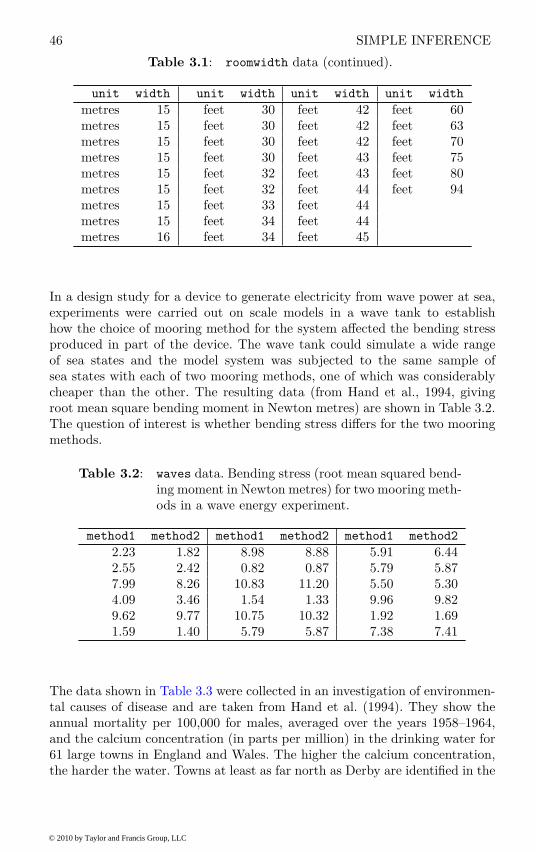
46 SIMPLE INFERENCE
Table 3.1: roomwidth data (continued).
unit width unit width unit width unit width
metres 15 feet 30 feet 42 feet 60metres 15 feet 30 feet 42 feet 63metres 15 feet 30 feet 42 feet 70metres 15 feet 30 feet 43 feet 75metres 15 feet 32 feet 43 feet 80metres 15 feet 32 feet 44 feet 94metres 15 feet 33 feet 44metres 15 feet 34 feet 44metres 16 feet 34 feet 45
In a design study for a device to generate electricity from wave power at sea,experiments were carried out on scale models in a wave tank to establishhow the choice of mooring method for the system affected the bending stressproduced in part of the device. The wave tank could simulate a wide rangeof sea states and the model system was subjected to the same sample ofsea states with each of two mooring methods, one of which was considerablycheaper than the other. The resulting data (from Hand et al., 1994, givingroot mean square bending moment in Newton metres) are shown in Table 3.2.The question of interest is whether bending stress differs for the two mooringmethods.
Table 3.2: waves data. Bending stress (root mean squared bend-ing moment in Newton metres) for two mooring meth-ods in a wave energy experiment.
method1 method2 method1 method2 method1 method2
2.23 1.82 8.98 8.88 5.91 6.442.55 2.42 0.82 0.87 5.79 5.877.99 8.26 10.83 11.20 5.50 5.304.09 3.46 1.54 1.33 9.96 9.829.62 9.77 10.75 10.32 1.92 1.691.59 1.40 5.79 5.87 7.38 7.41
The data shown in Table 3.3 were collected in an investigation of environmen-tal causes of disease and are taken from Hand et al. (1994). They show theannual mortality per 100,000 for males, averaged over the years 1958–1964,and the calcium concentration (in parts per million) in the drinking water for61 large towns in England and Wales. The higher the calcium concentration,the harder the water. Towns at least as far north as Derby are identified in the
© 2010 by Taylor and Francis Group, LLC

INTRODUCTION 47
table. Here there are several questions that might be of interest including: aremortality and water hardness related, and do either or both variables differbetween northern and southern towns?
Table 3.3: water data. Mortality (per 100,000 males per year,mortality) and water hardness for 61 cities in Eng-land and Wales.
location town mortality hardness
South Bath 1247 105North Birkenhead 1668 17South Birmingham 1466 5North Blackburn 1800 14North Blackpool 1609 18North Bolton 1558 10North Bootle 1807 15South Bournemouth 1299 78North Bradford 1637 10South Brighton 1359 84South Bristol 1392 73North Burnley 1755 12South Cardiff 1519 21South Coventry 1307 78South Croydon 1254 96North Darlington 1491 20North Derby 1555 39North Doncaster 1428 39South East Ham 1318 122South Exeter 1260 21North Gateshead 1723 44North Grimsby 1379 94North Halifax 1742 8North Huddersfield 1574 9North Hull 1569 91South Ipswich 1096 138North Leeds 1591 16South Leicester 1402 37North Liverpool 1772 15North Manchester 1828 8North Middlesbrough 1704 26North Newcastle 1702 44South Newport 1581 14South Northampton 1309 59South Norwich 1259 133North Nottingham 1427 27North Oldham 1724 6
© 2010 by Taylor and Francis Group, LLC

48 SIMPLE INFERENCE
Table 3.3: water data (continued).
location town mortality hardness
South Oxford 1175 107South Plymouth 1486 5South Portsmouth 1456 90North Preston 1696 6South Reading 1236 101North Rochdale 1711 13North Rotherham 1444 14North St Helens 1591 49North Salford 1987 8North Sheffield 1495 14South Southampton 1369 68South Southend 1257 50North Southport 1587 75North South Shields 1713 71North Stockport 1557 13North Stoke 1640 57North Sunderland 1709 71South Swansea 1625 13North Wallasey 1625 20South Walsall 1527 60South West Bromwich 1627 53South West Ham 1486 122South Wolverhampton 1485 81North York 1378 71
The two-way contingency table in Table 3.4 shows the number of piston-ringfailures in each of three legs of four steam-driven compressors located in thesame building (Haberman, 1973). The compressors have identical design andare oriented in the same way. The question of interest is whether the twocategorical variables (compressor and leg) are independent.
The data in Table 3.5 (taken from Agresti, 1996) arise from a sample ofjuveniles convicted of felony in Florida in 1987. Matched pairs were formedusing criteria such as age and the number of previous offences. For each pair,one subject was handled in the juvenile court and the other was transferred tothe adult court. Whether or not the juvenile was rearrested by the end of 1988was then noted. Here the question of interest is whether the true proportionsrearrested were identical for the adult and juvenile court assignments?
© 2010 by Taylor and Francis Group, LLC
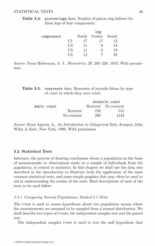
STATISTICAL TESTS 49
Table 3.4: pistonrings data. Number of piston ring failures forthree legs of four compressors.
leg
compressor North Centre SouthC1 17 17 12C2 11 9 13C3 11 8 19C4 14 7 28
Source: From Haberman, S. J., Biometrics, 29, 205–220, 1973. With permis-sion.
Table 3.5: rearrests data. Rearrests of juvenile felons by typeof court in which they were tried.
Juvenile court
Adult court Rearrest No rearrestRearrest 158 515
No rearrest 290 1134
Source: From Agresti, A., An Introduction to Categorical Data Analysis, JohnWiley & Sons, New York, 1996. With permission.
3.2 Statistical Tests
Inference, the process of drawing conclusions about a population on the basisof measurements or observations made on a sample of individuals from thepopulation, is central to statistics. In this chapter we shall use the data setsdescribed in the introduction to illustrate both the application of the mostcommon statistical tests, and some simple graphics that may often be used toaid in understanding the results of the tests. Brief descriptions of each of thetests to be used follow.
3.2.1 Comparing Normal Populations: Student’s t-Tests
The t-test is used to assess hypotheses about two population means wherethe measurements are assumed to be sampled from a normal distribution. Weshall describe two types of t-tests, the independent samples test and the pairedtest.
The independent samples t-test is used to test the null hypothesis that
© 2010 by Taylor and Francis Group, LLC

50 SIMPLE INFERENCE
the means of two populations are the same, H0 : µ1 = µ2, when a sample ofobservations from each population is available. The subjects of one populationmust not be individually matched with subjects from the other populationand the subjects within each group should not be related to each other. Thevariable to be compared is assumed to have a normal distribution with thesame standard deviation in both populations. The test statistic is essentiallya standardised difference of the two sample means,
t =y1 − y2
s√
1/n1 + 1/n2
(3.1)
where yi and ni are the means and sample sizes in groups i = 1 and 2,respectively. The pooled standard deviation s is given by
s =
√
(n1 − 1)s21
+ (n2 − 1)s22
n1 + n2 − 2
where s1 and s2 are the standard deviations in the two groups.Under the null hypothesis, the t-statistic has a Student’s t-distribution with
n1 + n2 − 2 degrees of freedom. A 100(1 − α)% confidence interval for thedifference between two means is useful in giving a plausible range of valuesfor the differences in the two means and is constructed as
y1 − y2 ± tα,n1+n2−2s
√
n−1
1+ n−1
2
where tα,n1+n2−2 is the percentage point of the t-distribution such that thecumulative distribution function, P(t ≤ tα,n1+n2−2), equals 1 − α/2.
If the two populations are suspected of having different variances, a modifiedform of the t statistic, known as the Welch test, may be used, namely
t =y1 − y2
√
s21/n1 + s2
2/n2
.
In this case, t has a Student’s t-distribution with ν degrees of freedom, where
ν =
(
c
n1 − 1+
(1 − c)2
n2 − 1
)
−1
with
c =s2
1/n1
s21/n1 + s2
2/n2
.
A paired t-test is used to compare the means of two populations whensamples from the populations are available, in which each individual in onesample is paired with an individual in the other sample or each individual inthe sample is observed twice. Examples of the former are anorexic girls andtheir healthy sisters and of the latter the same patients observed before andafter treatment.
If the values of the variable of interest, y, for the members of the ith pair ingroups 1 and 2 are denoted as y1i and y2i, then the differences di = y1i−y2i are
© 2010 by Taylor and Francis Group, LLC
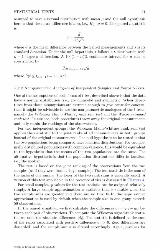
STATISTICAL TESTS 51
assumed to have a normal distribution with mean µ and the null hypothesishere is that the mean difference is zero, i.e., H0 : µ = 0. The paired t-statisticis
t =d
s/√
n
where d is the mean difference between the paired measurements and s is itsstandard deviation. Under the null hypothesis, t follows a t-distribution withn − 1 degrees of freedom. A 100(1 − α)% confidence interval for µ can beconstructed by
d ± tα,n−1s/√
n
where P(t ≤ tα,n−1) = 1 − α/2.
3.2.2 Non-parametric Analogues of Independent Samples and Paired t-Tests
One of the assumptions of both forms of t-test described above is that the datahave a normal distribution, i.e., are unimodal and symmetric. When depar-tures from those assumptions are extreme enough to give cause for concern,then it might be advisable to use the non-parametric analogues of the t-tests,namely the Wilcoxon Mann-Whitney rank sum test and the Wilcoxon signed
rank test. In essence, both procedures throw away the original measurementsand only retain the rankings of the observations.
For two independent groups, the Wilcoxon Mann-Whitney rank sum testapplies the t-statistic to the joint ranks of all measurements in both groupsinstead of the original measurements. The null hypothesis to be tested is thatthe two populations being compared have identical distributions. For two nor-mally distributed populations with common variance, this would be equivalentto the hypothesis that the means of the two populations are the same. Thealternative hypothesis is that the population distributions differ in location,i.e., the median.
The test is based on the joint ranking of the observations from the twosamples (as if they were from a single sample). The test statistic is the sum ofthe ranks of one sample (the lower of the two rank sums is generally used). Aversion of this test applicable in the presence of ties is discussed in Chapter 4.
For small samples, p-values for the test statistic can be assigned relativelysimply. A large sample approximation is available that is suitable when thetwo sample sizes are greater and there are no ties. In R, the large sampleapproximation is used by default when the sample size in one group exceeds50 observations.
In the paired situation, we first calculate the differences di = y1i − y2i be-tween each pair of observations. To compute the Wilcoxon signed-rank statis-tic, we rank the absolute differences |di|. The statistic is defined as the sumof the ranks associated with positive difference di > 0. Zero differences arediscarded, and the sample size n is altered accordingly. Again, p-values for
© 2010 by Taylor and Francis Group, LLC

52 SIMPLE INFERENCE
small sample sizes can be computed relatively simply and a large sample ap-proximation is available. It should be noted that this test is valid only whenthe differences di are symmetrically distributed.
3.2.3 Testing Independence in Contingency Tables
When a sample of n observations in two nominal (categorical) variables areavailable, they can be arranged into a cross-classification (see Table 3.6) inwhich the number of observations falling in each cell of the table is recorded.Table 3.6 is an example of such a contingency table, in which the observationsfor a sample of individuals or objects are cross-classified with respect to twocategorical variables. Testing for the independence of the two variables x andy is of most interest in general and details of the appropriate test follow.
Table 3.6: The general r × c table.
y
1 . . . c
1 n11 . . . n1c n1·
2 n21 . . . n2c n2·
x...
... . . ....
...r nr1 . . . nrc nr·
n·1 . . . n
·c n
Under the null hypothesis of independence of the row variable x and thecolumn variable y, estimated expected values Ejk for cell (j, k) can be com-puted from the corresponding margin totals Ejk = nj·n·k/n. The test statisticfor assessing independence is
X2 =r
∑
j=1
c∑
k=1
(njk − Ejk)2
Ejk
.
Under the null hypothesis of independence, the test statistic X2 is asymp-totically distributed according to a χ2-distribution with (r− 1)(c− 1) degreesof freedom, the corresponding test is usually known as chi-squared test.
3.2.4 McNemar’s Test
The chi-squared test on categorical data described previously assumes thatthe observations are independent. Often, however, categorical data arise frompaired observations, for example, cases matched with controls on variablessuch as gender, age and so on, or observations made on the same subjectson two occasions (cf. paired t-test). For this type of paired data, the required
© 2010 by Taylor and Francis Group, LLC
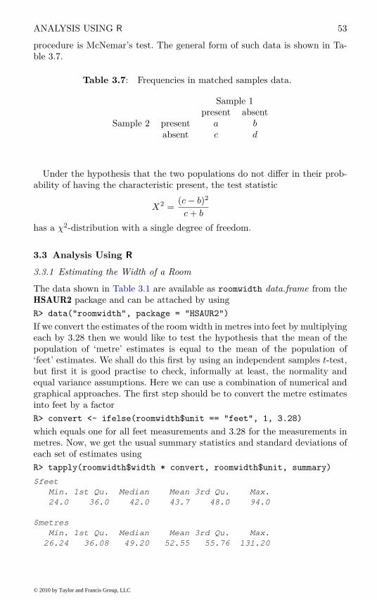
ANALYSIS USING R 53
procedure is McNemar’s test. The general form of such data is shown in Ta-ble 3.7.
Table 3.7: Frequencies in matched samples data.
Sample 1present absent
Sample 2 present a b
absent c d
Under the hypothesis that the two populations do not differ in their prob-ability of having the characteristic present, the test statistic
X2 =(c − b)2
c + b
has a χ2-distribution with a single degree of freedom.
3.3 Analysis Using R
3.3.1 Estimating the Width of a Room
The data shown in Table 3.1 are available as roomwidth data.frame from theHSAUR2 package and can be attached by using
R> data("roomwidth", package = "HSAUR2")
If we convert the estimates of the room width in metres into feet by multiplyingeach by 3.28 then we would like to test the hypothesis that the mean of thepopulation of ‘metre’ estimates is equal to the mean of the population of‘feet’ estimates. We shall do this first by using an independent samples t-test,but first it is good practise to check, informally at least, the normality andequal variance assumptions. Here we can use a combination of numerical andgraphical approaches. The first step should be to convert the metre estimatesinto feet by a factor
R> convert <- ifelse(roomwidth$unit == "feet", 1, 3.28)
which equals one for all feet measurements and 3.28 for the measurements inmetres. Now, we get the usual summary statistics and standard deviations ofeach set of estimates using
R> tapply(roomwidth$width * convert, roomwidth$unit, summary)
$feet
Min. 1st Qu. Median Mean 3rd Qu. Max.
24.0 36.0 42.0 43.7 48.0 94.0
$metres
Min. 1st Qu. Median Mean 3rd Qu. Max.
26.24 36.08 49.20 52.55 55.76 131.20
© 2010 by Taylor and Francis Group, LLC

54 SIMPLE INFERENCE
R> tapply(roomwidth$width * convert, roomwidth$unit, sd)
feet metres
12.49742 23.43444
where tapply applies summary, or sd, to the converted widths for both groupsof measurements given by roomwidth$unit. A boxplot of each set of estimatesmight be useful and is depicted in Figure 3.1. The layout function (line 1 inFigure 3.1) divides the plotting area in three parts. The boxplot functionproduces a boxplot in the upper part and the two qqnorm statements in lines8 and 11 set up the normal probability plots that can be used to assess thenormality assumption of the t-test.
The boxplots indicate that both sets of estimates contain a number of out-liers and also that the estimates made in metres are skewed and more variablethan those made in feet, a point underlined by the numerical summary statis-tics above. Both normal probability plots depart from linearity, suggesting thatthe distributions of both sets of estimates are not normal. The presence of out-liers, the apparently different variances and the evidence of non-normality allsuggest caution in applying the t-test, but for the moment we shall apply theusual version of the test using the t.test function in R.
The two-sample test problem is specified by a formula, here by
I(width * convert) ~ unit
where the response, width, on the left hand side needs to be converted firstand, because the star has a special meaning in formulae as will be explainedin Chapter 5, the conversion needs to be embedded by I. The factor unit onthe right hand side specifies the two groups to be compared.
From the output shown in Figure 3.2 we see that there is considerableevidence that the estimates made in feet are lower than those made in metresby between about 2 and 15 feet. The test statistic t from 3.1 is −2.615 and,with 111 degrees of freedom, the two-sided p-value is 0.01. In addition, a 95%confidence interval for the difference of the estimated widths between feet andmetres is reported.
But this form of t-test assumes both normality and equality of popula-tion variances, both of which are suspect for these data. Departure from theequality of variance assumption can be accommodated by the modified t-testdescribed above and this can be applied in R by choosing var.equal = FALSE
(note that var.equal = FALSE is the default in R). The result shown in Fig-ure 3.3 as well indicates that there is strong evidence for a difference in themeans of the two types of estimate.
But there remains the problem of the outliers and the possible non-normality;consequently we shall apply the Wilcoxon Mann-Whitney test which, since itis based on the ranks of the observations, is unlikely to be affected by theoutliers, and which does not assume that the data have a normal distribution.The test can be applied in R using the wilcox.test function.
Figure 3.4 shows a two-sided p-value of 0.028 confirming the difference inlocation of the two types of estimates of room width. Note that, due to ranking
© 2010 by Taylor and Francis Group, LLC

ANALYSIS USING R 55
1 R> layout(matrix(c(1,2,1,3), nrow = 2, ncol = 2, byrow = FALSE))
2 R> boxplot(I(width * convert) ~ unit, data = roomwidth,
3 + ylab = "Estimated width (feet)",
4 + varwidth = TRUE, names = c("Estimates in feet",
5 + "Estimates in metres (converted to feet)"))
6 R> feet <- roomwidth$unit == "feet"
7 R> qqnorm(roomwidth$width[feet],
8 + ylab = "Estimated width (feet)")
9 R> qqline(roomwidth$width[feet])
10 R> qqnorm(roomwidth$width[!feet],
11 + ylab = "Estimated width (metres)")
12 R> qqline(roomwidth$width[!feet])
Estimates in feet Estimates in metres (converted to feet)
20
40
60
80
10
0
Estim
ate
d w
idth
(fe
et)
−2 −1 0 1 2
30
50
70
90
Normal Q−Q Plot
Theoretical Quantiles
Estim
ate
d w
idth
(fe
et)
−2 −1 0 1 2
10
15
20
25
30
35
40
Normal Q−Q Plot
Theoretical Quantiles
Estim
ate
d w
idth
(m
etr
es)
Figure 3.1 Boxplots of estimates of room width in feet and metres (after conver-
sion to feet) and normal probability plots of estimates of room width
made in feet and in metres.
© 2010 by Taylor and Francis Group, LLC

56 SIMPLE INFERENCE
R> t.test(I(width * convert) ~ unit, data = roomwidth,
+ var.equal = TRUE)
Two Sample t-test
data: I(width * convert) by unit
t = -2.6147, df = 111, p-value = 0.01017
95 percent confidence interval:
-15.572734 -2.145052
sample estimates:
mean in group feet mean in group metres
43.69565 52.55455
Figure 3.2 R output of the independent samples t-test for the roomwidth data.
R> t.test(I(width * convert) ~ unit, data = roomwidth,
+ var.equal = FALSE)
Welch Two Sample t-test
data: I(width * convert) by unit
t = -2.3071, df = 58.788, p-value = 0.02459
95 percent confidence interval:
-16.54308 -1.17471
sample estimates:
mean in group feet mean in group metres
43.69565 52.55455
Figure 3.3 R output of the independent samples Welch test for the roomwidth
data.
the observations, the confidence interval for the median difference reportedhere is much smaller than the confidence interval for the difference in meansas shown in Figures 3.2 and 3.3. Further possible analyses of the data areconsidered in Exercise 3.1 and in Chapter 4.
3.3.2 Wave Energy Device Mooring
The data from Table 3.2 are available as data.frame waves
R> data("waves", package = "HSAUR2")
and requires the use of a matched pairs t-test to answer the question of inter-est. This test assumes that the differences between the matched observationshave a normal distribution so we can begin by checking this assumption byconstructing a boxplot and a normal probability plot – see Figure 3.5.
The boxplot indicates a possible outlier, and the normal probability plotgives little cause for concern about departures from normality, although with
© 2010 by Taylor and Francis Group, LLC

ANALYSIS USING R 57
R> wilcox.test(I(width * convert) ~ unit, data = roomwidth,
+ conf.int = TRUE)
Wilcoxon rank sum test with continuity correction
data: I(width * convert) by unit
W = 1145, p-value = 0.02815
95 percent confidence interval:
-9.3599953 -0.8000423
sample estimates:
difference in location
-5.279955
Figure 3.4 R output of the Wilcoxon rank sum test for the roomwidth data.
only 18 observations it is perhaps difficult to draw any convincing conclusion.We can now apply the paired t-test to the data again using the t.test func-tion. Figure 3.6 shows that there is no evidence for a difference in the meanbending stress of the two types of mooring device. Although there is no realreason for applying the non-parametric analogue of the paired t-test to thesedata, we give the R code for interest in Figure 3.7. The associated p-value is0.316 confirming the result from the t-test.
3.3.3 Mortality and Water Hardness
There is a wide range of analyses we could apply to the data in Table 3.3available from
R> data("water", package = "HSAUR2")
But to begin we will construct a scatterplot of the data enhanced somewhat bythe addition of information about the marginal distributions of water hardness(calcium concentration) and mortality, and by adding the estimated linearregression fit (see Chapter 6) for mortality on hardness. The plot and therequired R code is given along with Figure 3.8. In line 1 of Figure 3.8, wedivide the plotting region into four areas of different size. The scatterplot(line 3) uses a plotting symbol depending on the location of the city (by thepch argument); a legend for the location is added in line 6. We add a leastsquares fit (see Chapter 6) to the scatterplot and, finally, depict the marginaldistributions by means of a boxplot and a histogram. The scatterplot showsthat as hardness increases mortality decreases, and the histogram for the waterhardness shows it has a rather skewed distribution.
We can both calculate the Pearson’s correlation coefficient between the twovariables and test whether it differs significantly for zero by using the cor.test
function in R. The test statistic for assessing the hypothesis that the popula-tion correlation coefficient is zero is
r/√
(1 − r2)/(n − 2)
© 2010 by Taylor and Francis Group, LLC
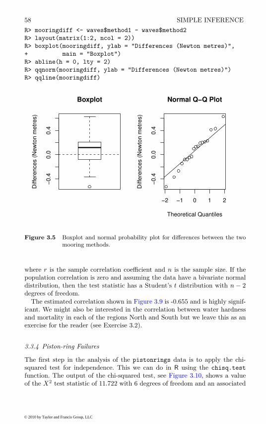
58 SIMPLE INFERENCE
R> mooringdiff <- waves$method1 - waves$method2
R> layout(matrix(1:2, ncol = 2))
R> boxplot(mooringdiff, ylab = "Differences (Newton metres)",
+ main = "Boxplot")
R> abline(h = 0, lty = 2)
R> qqnorm(mooringdiff, ylab = "Differences (Newton metres)")
R> qqline(mooringdiff)
−0
.40
.00
.4
Boxplot
Diffe
ren
ce
s (
New
ton
me
tre
s)
−2 −1 0 1 2
−0
.40
.00
.4
Normal Q−Q Plot
Theoretical Quantiles
Diffe
ren
ce
s (
New
ton
me
tre
s)
Figure 3.5 Boxplot and normal probability plot for differences between the two
mooring methods.
where r is the sample correlation coefficient and n is the sample size. If thepopulation correlation is zero and assuming the data have a bivariate normaldistribution, then the test statistic has a Student’s t distribution with n − 2degrees of freedom.
The estimated correlation shown in Figure 3.9 is -0.655 and is highly signif-icant. We might also be interested in the correlation between water hardnessand mortality in each of the regions North and South but we leave this as anexercise for the reader (see Exercise 3.2).
3.3.4 Piston-ring Failures
The first step in the analysis of the pistonrings data is to apply the chi-squared test for independence. This we can do in R using the chisq.test
function. The output of the chi-squared test, see Figure 3.10, shows a valueof the X2 test statistic of 11.722 with 6 degrees of freedom and an associated
© 2010 by Taylor and Francis Group, LLC
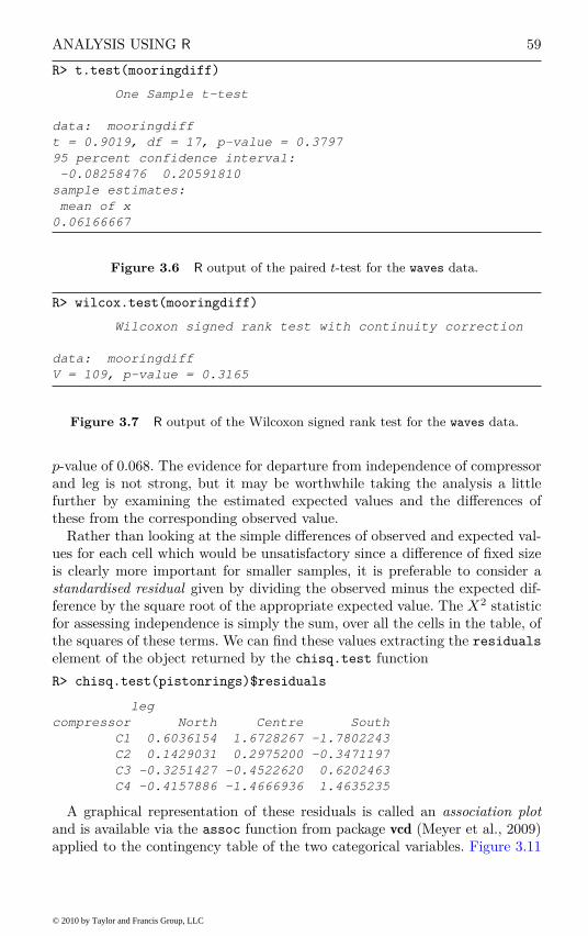
ANALYSIS USING R 59
R> t.test(mooringdiff)
One Sample t-test
data: mooringdiff
t = 0.9019, df = 17, p-value = 0.3797
95 percent confidence interval:
-0.08258476 0.20591810
sample estimates:
mean of x
0.06166667
Figure 3.6 R output of the paired t-test for the waves data.
R> wilcox.test(mooringdiff)
Wilcoxon signed rank test with continuity correction
data: mooringdiff
V = 109, p-value = 0.3165
Figure 3.7 R output of the Wilcoxon signed rank test for the waves data.
p-value of 0.068. The evidence for departure from independence of compressorand leg is not strong, but it may be worthwhile taking the analysis a littlefurther by examining the estimated expected values and the differences ofthese from the corresponding observed value.
Rather than looking at the simple differences of observed and expected val-ues for each cell which would be unsatisfactory since a difference of fixed sizeis clearly more important for smaller samples, it is preferable to consider astandardised residual given by dividing the observed minus the expected dif-ference by the square root of the appropriate expected value. The X2 statisticfor assessing independence is simply the sum, over all the cells in the table, ofthe squares of these terms. We can find these values extracting the residuals
element of the object returned by the chisq.test function
R> chisq.test(pistonrings)$residuals
leg
compressor North Centre South
C1 0.6036154 1.6728267 -1.7802243
C2 0.1429031 0.2975200 -0.3471197
C3 -0.3251427 -0.4522620 0.6202463
C4 -0.4157886 -1.4666936 1.4635235
A graphical representation of these residuals is called an association plot
and is available via the assoc function from package vcd (Meyer et al., 2009)applied to the contingency table of the two categorical variables. Figure 3.11
© 2010 by Taylor and Francis Group, LLC
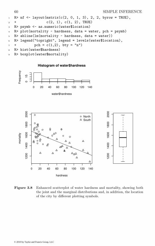
60 SIMPLE INFERENCE
1 R> nf <- layout(matrix(c(2, 0, 1, 3), 2, 2, byrow = TRUE),
2 + c(2, 1), c(1, 2), TRUE)
3 R> psymb <- as.numeric(water$location)
4 R> plot(mortality ~ hardness, data = water, pch = psymb)
5 R> abline(lm(mortality ~ hardness, data = water))
6 R> legend("topright", legend = levels(water$location),
7 + pch = c(1,2), bty = "n")
8 R> hist(water$hardness)
9 R> boxplot(water$mortality)
0 20 40 60 80 100 120 140
12
00
14
00
16
00
18
00
20
00
hardness
mo
rta
lity
NorthSouth
Histogram of water$hardness
water$hardness
Fre
qu
en
cy
0 20 40 60 80 100 120 140
01
5
12
00
14
00
16
00
18
00
20
00
Figure 3.8 Enhanced scatterplot of water hardness and mortality, showing both
the joint and the marginal distributions and, in addition, the location
of the city by different plotting symbols.
© 2010 by Taylor and Francis Group, LLC
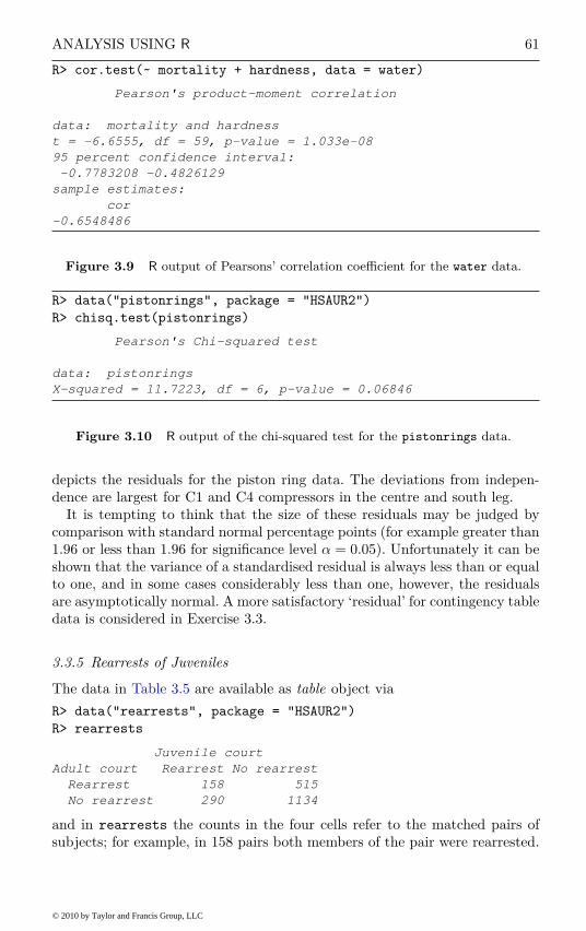
ANALYSIS USING R 61
R> cor.test(~ mortality + hardness, data = water)
Pearson's product-moment correlation
data: mortality and hardness
t = -6.6555, df = 59, p-value = 1.033e-08
95 percent confidence interval:
-0.7783208 -0.4826129
sample estimates:
cor
-0.6548486
Figure 3.9 R output of Pearsons’ correlation coefficient for the water data.
R> data("pistonrings", package = "HSAUR2")
R> chisq.test(pistonrings)
Pearson's Chi-squared test
data: pistonrings
X-squared = 11.7223, df = 6, p-value = 0.06846
Figure 3.10 R output of the chi-squared test for the pistonrings data.
depicts the residuals for the piston ring data. The deviations from indepen-dence are largest for C1 and C4 compressors in the centre and south leg.
It is tempting to think that the size of these residuals may be judged bycomparison with standard normal percentage points (for example greater than1.96 or less than 1.96 for significance level α = 0.05). Unfortunately it can beshown that the variance of a standardised residual is always less than or equalto one, and in some cases considerably less than one, however, the residualsare asymptotically normal. A more satisfactory ‘residual’ for contingency tabledata is considered in Exercise 3.3.
3.3.5 Rearrests of Juveniles
The data in Table 3.5 are available as table object via
R> data("rearrests", package = "HSAUR2")
R> rearrests
Juvenile court
Adult court Rearrest No rearrest
Rearrest 158 515
No rearrest 290 1134
and in rearrests the counts in the four cells refer to the matched pairs ofsubjects; for example, in 158 pairs both members of the pair were rearrested.
© 2010 by Taylor and Francis Group, LLC
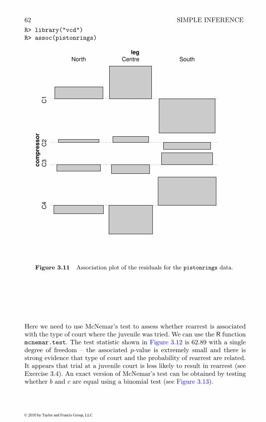
62 SIMPLE INFERENCE
R> library("vcd")
R> assoc(pistonrings)
leg
co
mp
res
so
rC
4C
3C
2C
1
North Centre South
Figure 3.11 Association plot of the residuals for the pistonrings data.
Here we need to use McNemar’s test to assess whether rearrest is associatedwith the type of court where the juvenile was tried. We can use the R functionmcnemar.test. The test statistic shown in Figure 3.12 is 62.89 with a singledegree of freedom – the associated p-value is extremely small and there isstrong evidence that type of court and the probability of rearrest are related.It appears that trial at a juvenile court is less likely to result in rearrest (seeExercise 3.4). An exact version of McNemar’s test can be obtained by testingwhether b and c are equal using a binomial test (see Figure 3.13).
© 2010 by Taylor and Francis Group, LLC
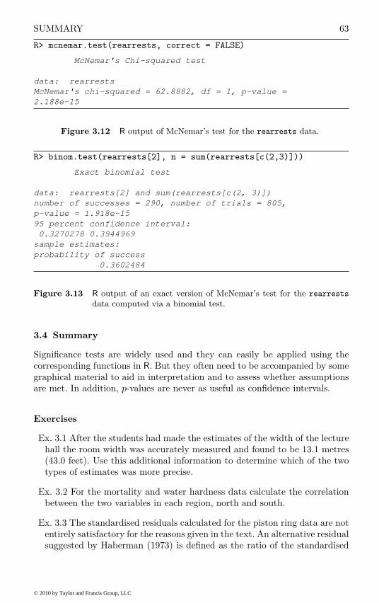
SUMMARY 63
R> mcnemar.test(rearrests, correct = FALSE)
McNemar's Chi-squared test
data: rearrests
McNemar's chi-squared = 62.8882, df = 1, p-value =
2.188e-15
Figure 3.12 R output of McNemar’s test for the rearrests data.
R> binom.test(rearrests[2], n = sum(rearrests[c(2,3)]))
Exact binomial test
data: rearrests[2] and sum(rearrests[c(2, 3)])
number of successes = 290, number of trials = 805,
p-value = 1.918e-15
95 percent confidence interval:
0.3270278 0.3944969
sample estimates:
probability of success
0.3602484
Figure 3.13 R output of an exact version of McNemar’s test for the rearrests
data computed via a binomial test.
3.4 Summary
Significance tests are widely used and they can easily be applied using thecorresponding functions in R. But they often need to be accompanied by somegraphical material to aid in interpretation and to assess whether assumptionsare met. In addition, p-values are never as useful as confidence intervals.
Exercises
Ex. 3.1 After the students had made the estimates of the width of the lecturehall the room width was accurately measured and found to be 13.1 metres(43.0 feet). Use this additional information to determine which of the twotypes of estimates was more precise.
Ex. 3.2 For the mortality and water hardness data calculate the correlationbetween the two variables in each region, north and south.
Ex. 3.3 The standardised residuals calculated for the piston ring data are notentirely satisfactory for the reasons given in the text. An alternative residualsuggested by Haberman (1973) is defined as the ratio of the standardised
© 2010 by Taylor and Francis Group, LLC

64 SIMPLE INFERENCE
residuals and an adjustment:√
(njk − Ejk)2/Ejk√
(1 − nj·/n)(1 − n·k/n)
.
When the variables forming the contingency table are independent, theadjusted residuals are approximately normally distributed with mean zeroand standard deviation one. Write a general R function to calculate bothstandardised and adjusted residuals for any r × c contingency table andapply it to the piston ring data.
Ex. 3.4 For the data in table rearrests estimate the difference betweenthe probability of being rearrested after being tried in an adult court andin a juvenile court, and find a 95% confidence interval for the populationdifference.
© 2010 by Taylor and Francis Group, LLC

CHAPTER 4
Conditional Inference: GuessingLengths, Suicides, Gastrointestinal
Damage, and Newborn Infants
4.1 Introduction
There are many experimental designs or studies where the subjects are nota random sample from some well-defined population. For example, subjectsrecruited for a clinical trial are hardly ever a random sample from the setof all people suffering from a certain disease but are a selection of patientsshowing up for examination in a hospital participating in the trial. Usually,the subjects are randomly assigned to certain groups, for example a controland a treatment group, and the analysis needs to take this randomisation intoaccount. In this chapter, we discuss such test procedures usually known as(re)-randomisation or permutation tests.
In the room width estimation experiment reported in Chapter 3, 40 of theestimated widths (in feet) of 69 students and 26 of the estimated widths (inmetres) of 44 students are tied. In fact, this violates one assumption of theunconditional test procedures applied in Chapter 3, namely that the measure-ments are drawn from a continuous distribution. In this chapter, the data willbe reanalysed using conditional test procedures, i.e., statistical tests wherethe distribution of the test statistics under the null hypothesis is determinedconditionally on the data at hand. A number of other data sets will also beconsidered in this chapter and these will now be described.
Mann (1981) reports a study carried out to investigate the causes of jeer-ing or baiting behaviour by a crowd when a person is threatening to commitsuicide by jumping from a high building. A hypothesis is that baiting is morelikely to occur in warm weather. Mann (1981) classified 21 accounts of threat-ened suicide by two factors, the time of year and whether or not baiting oc-curred. The data are given in Table 4.1 and the question is whether they giveany evidence to support the hypothesis? The data come from the northernhemisphere, so June–September are the warm months.
65
© 2010 by Taylor and Francis Group, LLC
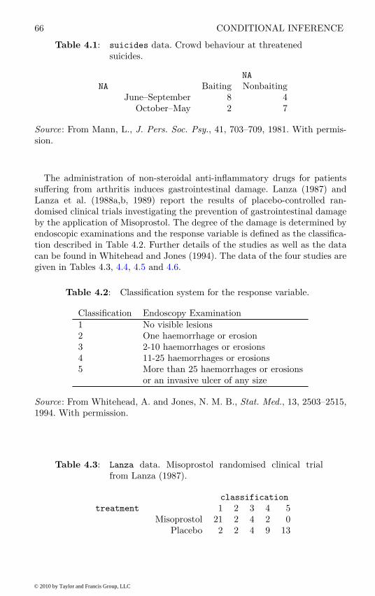
66 CONDITIONAL INFERENCE
Table 4.1: suicides data. Crowd behaviour at threatenedsuicides.
NA
NA Baiting NonbaitingJune–September 8 4
October–May 2 7
Source: From Mann, L., J. Pers. Soc. Psy., 41, 703–709, 1981. With permis-sion.
The administration of non-steroidal anti-inflammatory drugs for patientssuffering from arthritis induces gastrointestinal damage. Lanza (1987) andLanza et al. (1988a,b, 1989) report the results of placebo-controlled ran-domised clinical trials investigating the prevention of gastrointestinal damageby the application of Misoprostol. The degree of the damage is determined byendoscopic examinations and the response variable is defined as the classifica-tion described in Table 4.2. Further details of the studies as well as the datacan be found in Whitehead and Jones (1994). The data of the four studies aregiven in Tables 4.3, 4.4, 4.5 and 4.6.
Table 4.2: Classification system for the response variable.
Classification Endoscopy Examination1 No visible lesions2 One haemorrhage or erosion3 2-10 haemorrhages or erosions4 11-25 haemorrhages or erosions5 More than 25 haemorrhages or erosions
or an invasive ulcer of any size
Source: From Whitehead, A. and Jones, N. M. B., Stat. Med., 13, 2503–2515,1994. With permission.
Table 4.3: Lanza data. Misoprostol randomised clinical trialfrom Lanza (1987).
classification
treatment 1 2 3 4 5Misoprostol 21 2 4 2 0
Placebo 2 2 4 9 13
© 2010 by Taylor and Francis Group, LLC
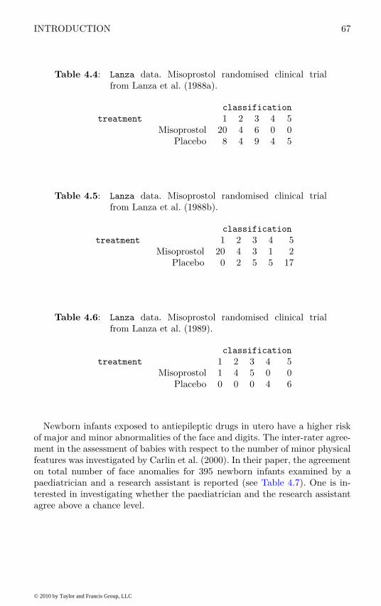
INTRODUCTION 67
Table 4.4: Lanza data. Misoprostol randomised clinical trialfrom Lanza et al. (1988a).
classification
treatment 1 2 3 4 5Misoprostol 20 4 6 0 0
Placebo 8 4 9 4 5
Table 4.5: Lanza data. Misoprostol randomised clinical trialfrom Lanza et al. (1988b).
classification
treatment 1 2 3 4 5Misoprostol 20 4 3 1 2
Placebo 0 2 5 5 17
Table 4.6: Lanza data. Misoprostol randomised clinical trialfrom Lanza et al. (1989).
classification
treatment 1 2 3 4 5Misoprostol 1 4 5 0 0
Placebo 0 0 0 4 6
Newborn infants exposed to antiepileptic drugs in utero have a higher riskof major and minor abnormalities of the face and digits. The inter-rater agree-ment in the assessment of babies with respect to the number of minor physicalfeatures was investigated by Carlin et al. (2000). In their paper, the agreementon total number of face anomalies for 395 newborn infants examined by apaediatrician and a research assistant is reported (see Table 4.7). One is in-terested in investigating whether the paediatrician and the research assistantagree above a chance level.
© 2010 by Taylor and Francis Group, LLC

68 CONDITIONAL INFERENCE
Table 4.7: anomalies data. Abnormalities of the face and digitsof newborn infants exposed to antiepileptic drugs asassessed by a paediatrician (MD) and a research assis-tant (RA).
RA
MD 0 1 2 30 235 41 20 21 23 35 11 12 3 8 11 33 0 0 1 1
Source: From Carlin, J. B., et al., Teratology, 62, 406-412, 2000. With permis-sion.
4.2 Conditional Test Procedures
The statistical test procedures applied in Chapter 3 all are defined for sam-ples randomly drawn from a well-defined population. In many experimentshowever, this model is far from being realistic. For example in clinical trials,it is often impossible to draw a random sample from all patients suffering acertain disease. Commonly, volunteers and patients are recruited from hos-pital staff, relatives or people showing up for some examination. The testprocedures applied in this chapter make no assumptions about random sam-pling or a specific model. Instead, the null distribution of the test statistics iscomputed conditionally on all random permutations of the data. Therefore,the procedures shown in the sequel are known as permutation tests or (re)-
randomisation tests. For a general introduction we refer to the text books ofEdgington (1987) and Pesarin (2001).
4.2.1 Testing Independence of Two Variables
Based on n pairs of measurements (xi, yi) recorded for n observational unitswe want to test the null hypothesis of the independence of x and y. We maydistinguish three situations: both variables x and y are continuous, one iscontinuous and the other one is a factor or both x and y are factors. Thespecial case of paired observations is treated in Section 4.2.2.
One class of test procedures for the above three situations are randomisationand permutation tests whose basic principles have been described by Fisher(1935) and Pitman (1937) and are best illustrated for the case of continuousmeasurements y in two groups, i.e., the x variable is a factor that can takevalues x = 1 or x = 2. The difference of the means of the y values in bothgroups is an appropriate statistic for the assessment of the association of y
© 2010 by Taylor and Francis Group, LLC

CONDITIONAL TEST PROCEDURES 69
and x
T =
n∑
i=1
I(xi = 1)yi
n∑
i=1
I(xi = 1)−
n∑
i=1
I(xi = 2)yi
n∑
i=1
I(xi = 2).
Here I(xi = 1) is the indication function which is equal to one if the condi-tion xi = 1 is true and zero otherwise. Clearly, under the null hypothesis ofindependence of x and y we expect the distribution of T to be centred aboutzero.
Suppose that the group labels x = 1 or x = 2 have been assigned to theobservational units by randomisation. When the result of the randomisationprocedure is independent of the y measurements, we are allowed to fix the xvalues and shuffle the y values randomly over and over again. Thus, we cancompute, or at least approximate, the distribution of the test statistic T underthe conditions of the null hypothesis directly from the data (xi, yi), i = 1, . . . , nby the so called randomisation principle. The test statistic T is computed fora reasonable number of shuffled y values and we can determine how many ofthe shuffled differences are at least as large as the test statistic T obtainedfrom the original data. If this proportion is small, smaller than α = 0.05 say,we have good evidence that the assumption of independence of x and y is notrealistic and we therefore can reject the null hypothesis. The proportion oflarger differences is usually referred to as p-value.
A special approach is based on ranks assigned to the continuous y values.When we replace the raw measurements yi by their corresponding ranks in thecomputation of T and compare this test statistic with its null distribution weend up with the Wilcoxon Mann-Whitney rank sum test. The conditional dis-tribution and the unconditional distribution of the Wilcoxon Mann-Whitneyrank sum test as introduced in Chapter 3 coincide when the y values are nottied. Without ties in the y values, the ranks are simply the integers 1, 2, . . . , nand the unconditional (Chapter 3) and the conditional view on the WilcoxonMann-Whitney test coincide.
In the case that both variables are nominal, the test statistic can be com-puted from the corresponding contingency table in which the observations(xi, yi) are cross-classified. A general r × c contingency table may be writ-ten in the form of Table 3.6 where each cell (j, k) is the number nij =∑n
i=1I(xi = j)I(yi = k), see Chapter 3 for more details.
Under the null hypothesis of independence of x and y, estimated expectedvalues Ejk for cell (j, k) can be computed from the corresponding margintotals Ejk = nj·n·k/n which are fixed for each randomisation of the data. Thetest statistic for assessing independence is
X2 =r
∑
j=1
c∑
k=1
(njk − Ejk)2
Ejk
.
The exact distribution based on all permutations of the y values for a similar
© 2010 by Taylor and Francis Group, LLC

70 CONDITIONAL INFERENCE
test statistic can be computed by means of Fisher’s exact test (Freeman andHalton, 1951). This test procedure is based on the hyper-geometric probabilityof the observed contingency table. All possible tables can be ordered withrespect to this metric and p-values are computed from the fraction of tablesmore extreme than the observed one.
When both the x and the y measurements are numeric, the test statisticcan be formulated as the product, i.e., by the sum of all xiyi, i = 1, . . . , n.Again, we can fix the x values and shuffle the y values in order to approximatethe distribution of the test statistic under the laws of the null hypothesis ofindependence of x and y.
4.2.2 Testing Marginal Homogeneity
In contrast to the independence problem treated above the data analyst isoften confronted with situations where two (or more) measurements of onevariable taken from the same observational unit are to be compared. In thiscase one assumes that the measurements are independent between observa-tions and the test statistics are aggregated over all observations. Where twonominal variables are taken for each observation (for example see the case ofMcNemar’s test for binary variables as discussed in Chapter 3), the measure-ment of each observation can be summarised by a k× k matrix with cell (i, j)being equal to one if the first measurement is the ith level and the second mea-surement is the jth level. All other entries are zero. Under the null hypothesisof independence of the first and second measurement, all k × k matrices withexactly one non-zero element are equally likely. The test statistic is now basedon the elementwise sum of all n matrices.
4.3 Analysis Using R
4.3.1 Estimating the Width of a Room Revised
The unconditional analysis of the room width estimated by two groups ofstudents in Chapter 3 led to the conclusion that the estimates in metres areslightly larger than the estimates in feet. Here, we reanalyse these data in aconditional framework. First, we convert metres into feet and store the vectorof observations in a variable y:
R> data("roomwidth", package = "HSAUR2")
R> convert <- ifelse(roomwidth$unit == "feet", 1, 3.28)
R> feet <- roomwidth$unit == "feet"
R> metre <- !feet
R> y <- roomwidth$width * convert
The test statistic is simply the difference in means
R> T <- mean(y[feet]) - mean(y[metre])
R> T
[1] -8.858893
© 2010 by Taylor and Francis Group, LLC
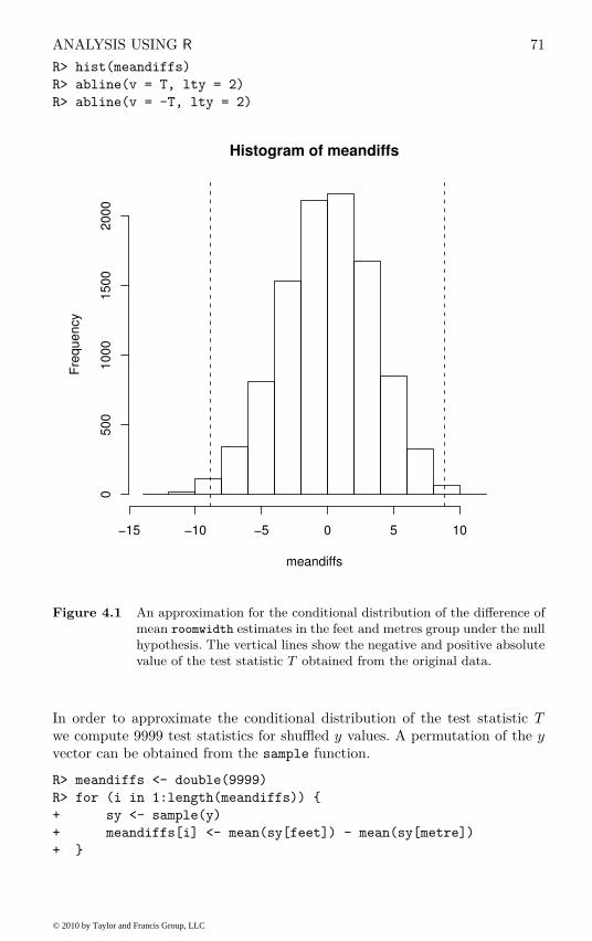
ANALYSIS USING R 71
R> hist(meandiffs)
R> abline(v = T, lty = 2)
R> abline(v = -T, lty = 2)
Histogram of meandiffs
meandiffs
Fre
qu
en
cy
−15 −10 −5 0 5 10
05
00
10
00
15
00
20
00
Figure 4.1 An approximation for the conditional distribution of the difference of
mean roomwidth estimates in the feet and metres group under the null
hypothesis. The vertical lines show the negative and positive absolute
value of the test statistic T obtained from the original data.
In order to approximate the conditional distribution of the test statistic Twe compute 9999 test statistics for shuffled y values. A permutation of the yvector can be obtained from the sample function.
R> meandiffs <- double(9999)
R> for (i in 1:length(meandiffs)) {
+ sy <- sample(y)
+ meandiffs[i] <- mean(sy[feet]) - mean(sy[metre])
+ }
© 2010 by Taylor and Francis Group, LLC
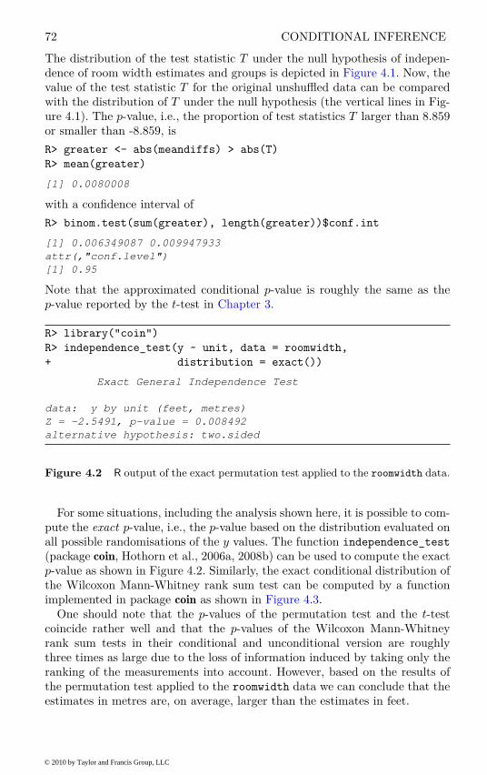
72 CONDITIONAL INFERENCE
The distribution of the test statistic T under the null hypothesis of indepen-dence of room width estimates and groups is depicted in Figure 4.1. Now, thevalue of the test statistic T for the original unshuffled data can be comparedwith the distribution of T under the null hypothesis (the vertical lines in Fig-ure 4.1). The p-value, i.e., the proportion of test statistics T larger than 8.859or smaller than -8.859, is
R> greater <- abs(meandiffs) > abs(T)
R> mean(greater)
[1] 0.0080008
with a confidence interval of
R> binom.test(sum(greater), length(greater))$conf.int
[1] 0.006349087 0.009947933
attr(,"conf.level")
[1] 0.95
Note that the approximated conditional p-value is roughly the same as thep-value reported by the t-test in Chapter 3.
R> library("coin")
R> independence_test(y ~ unit, data = roomwidth,
+ distribution = exact())
Exact General Independence Test
data: y by unit (feet, metres)
Z = -2.5491, p-value = 0.008492
alternative hypothesis: two.sided
Figure 4.2 R output of the exact permutation test applied to the roomwidth data.
For some situations, including the analysis shown here, it is possible to com-pute the exact p-value, i.e., the p-value based on the distribution evaluated onall possible randomisations of the y values. The function independence_test
(package coin, Hothorn et al., 2006a, 2008b) can be used to compute the exactp-value as shown in Figure 4.2. Similarly, the exact conditional distribution ofthe Wilcoxon Mann-Whitney rank sum test can be computed by a functionimplemented in package coin as shown in Figure 4.3.
One should note that the p-values of the permutation test and the t-testcoincide rather well and that the p-values of the Wilcoxon Mann-Whitneyrank sum tests in their conditional and unconditional version are roughlythree times as large due to the loss of information induced by taking only theranking of the measurements into account. However, based on the results ofthe permutation test applied to the roomwidth data we can conclude that theestimates in metres are, on average, larger than the estimates in feet.
© 2010 by Taylor and Francis Group, LLC

ANALYSIS USING R 73
R> wilcox_test(y ~ unit, data = roomwidth,
+ distribution = exact())
Exact Wilcoxon Mann-Whitney Rank Sum Test
data: y by unit (feet, metres)
Z = -2.1981, p-value = 0.02763
alternative hypothesis: true mu is not equal to 0
Figure 4.3 R output of the exact conditional Wilcoxon rank sum test applied to
the roomwidth data.
4.3.2 Crowds and Threatened Suicide
The data in this case are in the form of a 2 × 2 contingency table and itmight be thought that the chi-squared test could again be applied to testfor the independence of crowd behaviour and time of year. However, the χ2-distribution as an approximation to the independence test statistic is bad whenthe expected frequencies are rather small. The problem is discussed in detailin Everitt (1992) and Agresti (1996). One solution is to use a conditional testprocedure such as Fisher’s exact test as described above. We can apply thistest procedure using the R function fisher.test to the table suicides (seeFigure 4.4).
R> data("suicides", package = "HSAUR2")
R> fisher.test(suicides)
Fisher's Exact Test for Count Data
data: suicides
p-value = 0.0805
alternative hypothesis: true odds ratio is not equal to 1
95 percent confidence interval:
0.7306872 91.0288231
sample estimates:
odds ratio
6.302622
Figure 4.4 R output of Fisher’s exact test for the suicides data.
The resulting p-value obtained from the hypergeometric distribution is 0.08(the asymptotic p-value associated with the X2 statistic for this table is 0.115).There is no strong evidence of crowd behaviour being associated with time ofyear of threatened suicide, but the sample size is low and the test lacks power.Fisher’s exact test can also be applied to larger than 2 × 2 tables, especiallywhen there is concern that the cell frequencies are low (see Exercise 4.1).
© 2010 by Taylor and Francis Group, LLC

74 CONDITIONAL INFERENCE
4.3.3 Gastrointestinal Damage
Here we are interested in the comparison of two groups of patients, where onegroup received a placebo and the other one Misoprostol. In the trials shownhere, the response variable is measured on an ordered scale – see Table 4.2.Data from four clinical studies are available and thus the observations arenaturally grouped together. From the data.frame Lanza we can construct athree-way table as follows:
R> data("Lanza", package = "HSAUR2")
R> xtabs(~ treatment + classification + study, data = Lanza)
, , study = I
classification
treatment 1 2 3 4 5
Misoprostol 21 2 4 2 0
Placebo 2 2 4 9 13
, , study = II
classification
treatment 1 2 3 4 5
Misoprostol 20 4 6 0 0
Placebo 8 4 9 4 5
, , study = III
classification
treatment 1 2 3 4 5
Misoprostol 20 4 3 1 2
Placebo 0 2 5 5 17
, , study = IV
classification
treatment 1 2 3 4 5
Misoprostol 1 4 5 0 0
Placebo 0 0 0 4 6
We will first analyse each study separately and then show how one caninvestigate the effect of Misoprostol for all four studies simultaneously. Becausethe response is ordered, we take this information into account by assigning ascore to each level of the response. Since the classifications are defined by thenumber of haemorrhages or erosions, the midpoint of the interval for each levelis a reasonable choice, i.e., 0, 1, 6, 17 and 30 – compare those scores to thedefinitions given in Table 4.2. The corresponding linear-by-linear associationtests extending the general Cochran-Mantel-Haenszel statistics (see Agresti,2002, for further details) are implemented in package coin.
© 2010 by Taylor and Francis Group, LLC
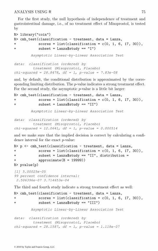
ANALYSIS USING R 75
For the first study, the null hypothesis of independence of treatment andgastrointestinal damage, i.e., of no treatment effect of Misoprostol, is testedby
R> library("coin")
R> cmh_test(classification ~ treatment, data = Lanza,
+ scores = list(classification = c(0, 1, 6, 17, 30)),
+ subset = Lanza$study == "I")
Asymptotic Linear-by-Linear Association Test
data: classification (ordered) by
treatment (Misoprostol, Placebo)
chi-squared = 28.8478, df = 1, p-value = 7.83e-08
and, by default, the conditional distribution is approximated by the corre-sponding limiting distribution. The p-value indicates a strong treatment effect.For the second study, the asymptotic p-value is a little bit larger:
R> cmh_test(classification ~ treatment, data = Lanza,
+ scores = list(classification = c(0, 1, 6, 17, 30)),
+ subset = Lanza$study == "II")
Asymptotic Linear-by-Linear Association Test
data: classification (ordered) by
treatment (Misoprostol, Placebo)
chi-squared = 12.0641, df = 1, p-value = 0.000514
and we make sure that the implied decision is correct by calculating a confi-dence interval for the exact p-value:
R> p <- cmh_test(classification ~ treatment, data = Lanza,
+ scores = list(classification = c(0, 1, 6, 17, 30)),
+ subset = Lanza$study == "II", distribution =
+ approximate(B = 19999))
R> pvalue(p)
[1] 5.00025e-05
99 percent confidence interval:
2.506396e-07 3.714653e-04
The third and fourth study indicate a strong treatment effect as well:
R> cmh_test(classification ~ treatment, data = Lanza,
+ scores = list(classification = c(0, 1, 6, 17, 30)),
+ subset = Lanza$study == "III")
Asymptotic Linear-by-Linear Association Test
data: classification (ordered) by
treatment (Misoprostol, Placebo)
chi-squared = 28.1587, df = 1, p-value = 1.118e-07
© 2010 by Taylor and Francis Group, LLC

76 CONDITIONAL INFERENCE
R> cmh_test(classification ~ treatment, data = Lanza,
+ scores = list(classification = c(0, 1, 6, 17, 30)),
+ subset = Lanza$study == "IV")
Asymptotic Linear-by-Linear Association Test
data: classification (ordered) by
treatment (Misoprostol, Placebo)
chi-squared = 15.7414, df = 1, p-value = 7.262e-05
At the end, a separate analysis for each study is unsatisfactory. Because thedesign of the four studies is the same, we can use study as a block variableand perform a global linear-association test investigating the treatment effectof Misoprostol in all four studies. The block variable can be incorporated intothe formula by the | symbol.
R> cmh_test(classification ~ treatment | study, data = Lanza,
+ scores = list(classification = c(0, 1, 6, 17, 30)))
Asymptotic Linear-by-Linear Association Test
data: classification (ordered) by
treatment (Misoprostol, Placebo)
stratified by study
chi-squared = 83.6188, df = 1, p-value < 2.2e-16
Based on this result, a strong treatment effect can be established.
4.3.4 Teratogenesis
In this example, the medical doctor (MD) and the research assistant (RA)assessed the number of anomalies (0, 1, 2 or 3) for each of 395 babies:
R> anomalies <- c(235, 23, 3, 0, 41, 35, 8, 0,
+ 20, 11, 11, 1, 2, 1, 3, 1)
R> anomalies <- as.table(matrix(anomalies,
+ ncol = 4, dimnames = list(MD = 0:3, RA = 0:3)))
R> anomalies
RA
MD 0 1 2 3
0 235 41 20 2
1 23 35 11 1
2 3 8 11 3
3 0 0 1 1
We are interested in testing whether the number of anomalies assessed by themedical doctor differs structurally from the number reported by the researchassistant. Because we compare paired observations, i.e., one pair of measure-ments for each newborn, a test of marginal homogeneity (a generalisation ofMcNemar’s test, Chapter 3) needs to be applied:
© 2010 by Taylor and Francis Group, LLC

SUMMARY 77
R> mh_test(anomalies)
Asymptotic Marginal-Homogeneity Test
data: response by
groups (MD, RA)
stratified by block
chi-squared = 21.2266, df = 3, p-value = 9.446e-05
The p-value indicates a deviation from the null hypothesis. However, the levelsof the response are not treated as ordered. Similar to the analysis of thegastrointestinal damage data above, we can take this information into accountby the definition of an appropriate score. Here, the number of anomalies is anatural choice:
R> mh_test(anomalies, scores = list(c(0, 1, 2, 3)))
Asymptotic Marginal-Homogeneity Test for Ordered Data
data: response (ordered) by
groups (MD, RA)
stratified by block
chi-squared = 21.0199, df = 1, p-value = 4.545e-06
In our case, both versions coincide and one can conclude that the assessment ofthe number of anomalies differs between the medical doctor and the researchassistant.
4.4 Summary
The analysis of randomised experiments, for example the analysis of ran-domised clinical trials such as the Misoprostol trial presented in this chapter,requires the application of conditional inferences procedures. In such experi-ments, the observations might not have been sampled from well-defined pop-ulations but are assigned to treatment groups, say, by a random procedurewhich is reiterated when randomisation tests are applied.
Exercises
Ex. 4.1 Although in the past Fisher’s test has been largely applied to sparse2 × 2 tables, it can also be applied to larger tables, especially when thereis concern about small values in some cells. Using the data displayed inTable 4.8 (taken from Mehta and Patel, 2003) which gives the distributionof the oral lesion site found in house-to-house surveys in three geographicregions of rural India, find the p-value from Fisher’s test and the correspond-ing p-value from applying the usual chi-square test to the data. What areyour conclusions?
© 2010 by Taylor and Francis Group, LLC

78 CONDITIONAL INFERENCE
Table 4.8: orallesions data. Oral lesions found in house-to-house surveys in three geographic regions of rural In-dia.
region
site of lesion Kerala Gujarat AndhraBuccal mucosa 8 1 8
Commissure 0 1 0Gingiva 0 1 0
Hard palate 0 1 0Soft palate 0 1 0
Tongue 0 1 0Floor of mouth 1 0 1Alveolar ridge 1 0 1
Source: From Mehta, C. and Patel, N., StatXact-6: Statistical Software for
Exact Nonparametric Inference, Cytel Software Corporation, Cambridge,MA, 2003. With permission.
Ex. 4.2 Use the mosaic and assoc functions from the vcd package (Meyeret al., 2009) to create a graphical representation of the deviations fromindependence in the 2 × 2 contingency table shown in Table 4.1.
Ex. 4.3 Generate two groups with measurements following a normal distri-bution having different means. For multiple replications of this experiment(1000, say), compare the p-values of the Wilcoxon Mann-Whitney ranksum test and a permutation test (using independence_test). Where dothe differences come from?
© 2010 by Taylor and Francis Group, LLC

CHAPTER 5
Analysis of Variance: Weight Gain,Foster Feeding in Rats, Water
Hardness and Male Egyptian Skulls
5.1 Introduction
The data in Table 5.1 (from Hand et al., 1994) arise from an experiment tostudy the gain in weight of rats fed on four different diets, distinguished byamount of protein (low and high) and by source of protein (beef and cereal).Ten rats are randomised to each of the four treatments and the weight gainin grams recorded. The question of interest is how diet affects weight gain.
Table 5.1: weightgain data. Rat weight gain for diets differingby the amount of protein (type) and source of protein(source).
source type weightgain source type weightgain
Beef Low 90 Cereal Low 107Beef Low 76 Cereal Low 95Beef Low 90 Cereal Low 97Beef Low 64 Cereal Low 80Beef Low 86 Cereal Low 98Beef Low 51 Cereal Low 74Beef Low 72 Cereal Low 74Beef Low 90 Cereal Low 67Beef Low 95 Cereal Low 89Beef Low 78 Cereal Low 58Beef High 73 Cereal High 98Beef High 102 Cereal High 74Beef High 118 Cereal High 56Beef High 104 Cereal High 111Beef High 81 Cereal High 95Beef High 107 Cereal High 88Beef High 100 Cereal High 82Beef High 87 Cereal High 77Beef High 117 Cereal High 86Beef High 111 Cereal High 92
79
© 2010 by Taylor and Francis Group, LLC

80 ANALYSIS OF VARIANCE
The data in Table 5.2 are from a foster feeding experiment with rat mothersand litters of four different genotypes: A, B, I and J (Hand et al., 1994). Themeasurement is the litter weight (in grams) after a trial feeding period. Herethe investigator’s interest lies in uncovering the effect of genotype of motherand litter on litter weight.
Table 5.2: foster data. Foster feeding experiment for rats withdifferent genotypes of the litter (litgen) and mother(motgen).
litgen motgen weight litgen motgen weight
A A 61.5 B J 40.5A A 68.2 I A 37.0A A 64.0 I A 36.3A A 65.0 I A 68.0A A 59.7 I B 56.3A B 55.0 I B 69.8A B 42.0 I B 67.0A B 60.2 I I 39.7A I 52.5 I I 46.0A I 61.8 I I 61.3A I 49.5 I I 55.3A I 52.7 I I 55.7A J 42.0 I J 50.0A J 54.0 I J 43.8A J 61.0 I J 54.5A J 48.2 J A 59.0A J 39.6 J A 57.4B A 60.3 J A 54.0B A 51.7 J A 47.0B A 49.3 J B 59.5B A 48.0 J B 52.8B B 50.8 J B 56.0B B 64.7 J I 45.2B B 61.7 J I 57.0B B 64.0 J I 61.4B B 62.0 J J 44.8B I 56.5 J J 51.5B I 59.0 J J 53.0B I 47.2 J J 42.0B I 53.0 J J 54.0B J 51.3
© 2010 by Taylor and Francis Group, LLC

INTRODUCTION 81
The data in Table 5.3 (from Hand et al., 1994) give four measurements madeon Egyptian skulls from five epochs. The data has been collected with a viewto deciding if there are any differences between the skulls from the five epochs.The measurements are:
mb: maximum breadths of the skull,
bh: basibregmatic heights of the skull,
bl: basialiveolar length of the skull, and
nh: nasal heights of the skull.
Non-constant measurements of the skulls over time would indicate interbreed-ing with immigrant populations.
Table 5.3: skulls data. Measurements of four variables takenfrom Egyptian skulls of five periods.
epoch mb bh bl nh
c4000BC 131 138 89 49c4000BC 125 131 92 48c4000BC 131 132 99 50c4000BC 119 132 96 44c4000BC 136 143 100 54c4000BC 138 137 89 56c4000BC 139 130 108 48c4000BC 125 136 93 48c4000BC 131 134 102 51c4000BC 134 134 99 51c4000BC 129 138 95 50c4000BC 134 121 95 53c4000BC 126 129 109 51c4000BC 132 136 100 50c4000BC 141 140 100 51c4000BC 131 134 97 54c4000BC 135 137 103 50c4000BC 132 133 93 53c4000BC 139 136 96 50c4000BC 132 131 101 49c4000BC 126 133 102 51c4000BC 135 135 103 47c4000BC 134 124 93 53
......
......
...
© 2010 by Taylor and Francis Group, LLC
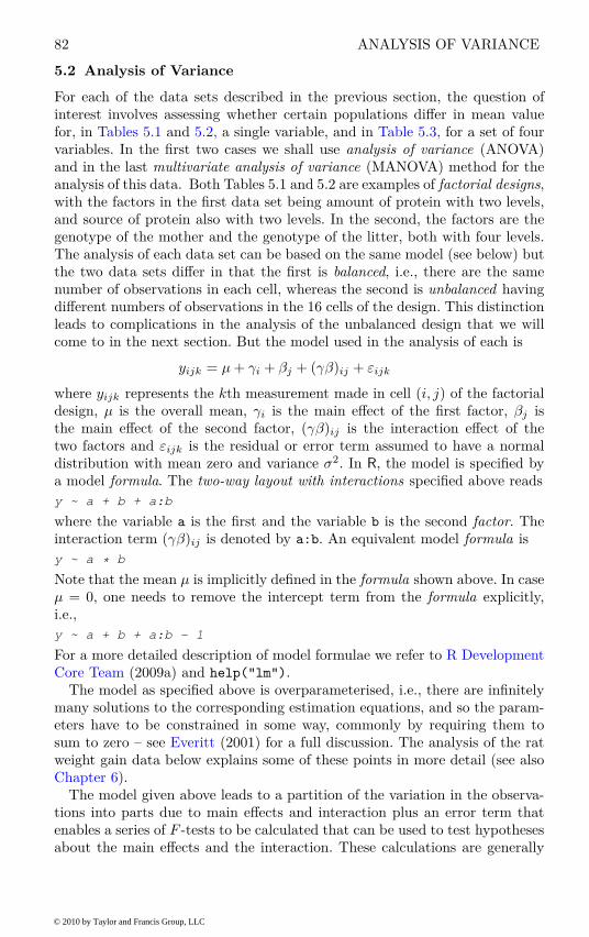
82 ANALYSIS OF VARIANCE
5.2 Analysis of Variance
For each of the data sets described in the previous section, the question ofinterest involves assessing whether certain populations differ in mean valuefor, in Tables 5.1 and 5.2, a single variable, and in Table 5.3, for a set of fourvariables. In the first two cases we shall use analysis of variance (ANOVA)and in the last multivariate analysis of variance (MANOVA) method for theanalysis of this data. Both Tables 5.1 and 5.2 are examples of factorial designs,with the factors in the first data set being amount of protein with two levels,and source of protein also with two levels. In the second, the factors are thegenotype of the mother and the genotype of the litter, both with four levels.The analysis of each data set can be based on the same model (see below) butthe two data sets differ in that the first is balanced, i.e., there are the samenumber of observations in each cell, whereas the second is unbalanced havingdifferent numbers of observations in the 16 cells of the design. This distinctionleads to complications in the analysis of the unbalanced design that we willcome to in the next section. But the model used in the analysis of each is
yijk = µ + γi + βj + (γβ)ij + εijk
where yijk represents the kth measurement made in cell (i, j) of the factorialdesign, µ is the overall mean, γi is the main effect of the first factor, βj isthe main effect of the second factor, (γβ)ij is the interaction effect of thetwo factors and εijk is the residual or error term assumed to have a normaldistribution with mean zero and variance σ2. In R, the model is specified bya model formula. The two-way layout with interactions specified above reads
y ~ a + b + a:b
where the variable a is the first and the variable b is the second factor. Theinteraction term (γβ)ij is denoted by a:b. An equivalent model formula is
y ~ a * b
Note that the mean µ is implicitly defined in the formula shown above. In caseµ = 0, one needs to remove the intercept term from the formula explicitly,i.e.,
y ~ a + b + a:b - 1
For a more detailed description of model formulae we refer to R DevelopmentCore Team (2009a) and help("lm").
The model as specified above is overparameterised, i.e., there are infinitelymany solutions to the corresponding estimation equations, and so the param-eters have to be constrained in some way, commonly by requiring them tosum to zero – see Everitt (2001) for a full discussion. The analysis of the ratweight gain data below explains some of these points in more detail (see alsoChapter 6).
The model given above leads to a partition of the variation in the observa-tions into parts due to main effects and interaction plus an error term thatenables a series of F -tests to be calculated that can be used to test hypothesesabout the main effects and the interaction. These calculations are generally
© 2010 by Taylor and Francis Group, LLC

ANALYSIS USING R 83
set out in the familiar analysis of variance table. The assumptions made inderiving the F -tests are:
• The observations are independent of each other,
• The observations in each cell arise from a population having a normal dis-tribution, and
• The observations in each cell are from populations having the same vari-ance.
The multivariate analysis of variance, or MANOVA, is an extension of theunivariate analysis of variance to the situation where a set of variables aremeasured on each individual or object observed. For the data in Table 5.3there is a single factor, epoch, and four measurements taken on each skull; sowe have a one-way MANOVA design. The linear model used in this case is
yijh = µh + γjh + εijh
where µh is the overall mean for variable h, γjh is the effect of the jth levelof the single factor on the hth variable, and εijh is a random error term. Thevector ε⊤ij = (εij1, εij2, . . . , εijq) where q is the number of response variables(four in the skull example) is assumed to have a multivariate normal distri-bution with null mean vector and covariance matrix, Σ, assumed to be thesame in each level of the grouping factor. The hypothesis of interest is thatthe population mean vectors for the different levels of the grouping factor arethe same.
In the multivariate situation, when there are more than two levels of thegrouping factor, no single test statistic can be derived which is always the mostpowerful, for all types of departures from the null hypothesis of the equalityof mean vector. A number of different test statistics are available which maygive different results when applied to the same data set, although the finalconclusion is often the same. The principal test statistics for the multivariateanalysis of variance are Hotelling-Lawley trace, Wilks’ ratio of determinants,Roy’s greatest root, and the Pillai trace. Details are given in Morrison (2005).
5.3 Analysis Using R
5.3.1 Weight Gain in Rats
Before applying analysis of variance to the data in Table 5.1 we should try tosummarise the main features of the data by calculating means and standarddeviations and by producing some hopefully informative graphs. The data isavailable in the data.frame weightgain. The following R code produces therequired summary statistics
R> data("weightgain", package = "HSAUR2")
R> tapply(weightgain$weightgain,
+ list(weightgain$source, weightgain$type), mean)
© 2010 by Taylor and Francis Group, LLC

84 ANALYSIS OF VARIANCE
R> plot.design(weightgain)
82
84
86
88
90
92
Factors
me
an
of
we
igh
tga
in
Beef
Cereal
High
Low
source type
Figure 5.1 Plot of mean weight gain for each level of the two factors.
High Low
Beef 100.0 79.2
Cereal 85.9 83.9
R> tapply(weightgain$weightgain,
+ list(weightgain$source, weightgain$type), sd)
High Low
Beef 15.13642 13.88684
Cereal 15.02184 15.70881
The cell variances are relatively similar and there is no apparent relationshipbetween cell mean and cell variance so the homogeneity assumption of theanalysis of variance looks like it is reasonable for these data. The plot of cellmeans in Figure 5.1 suggests that there is a considerable difference in weightgain for the amount of protein factor with the gain for the high-protein diet
© 2010 by Taylor and Francis Group, LLC
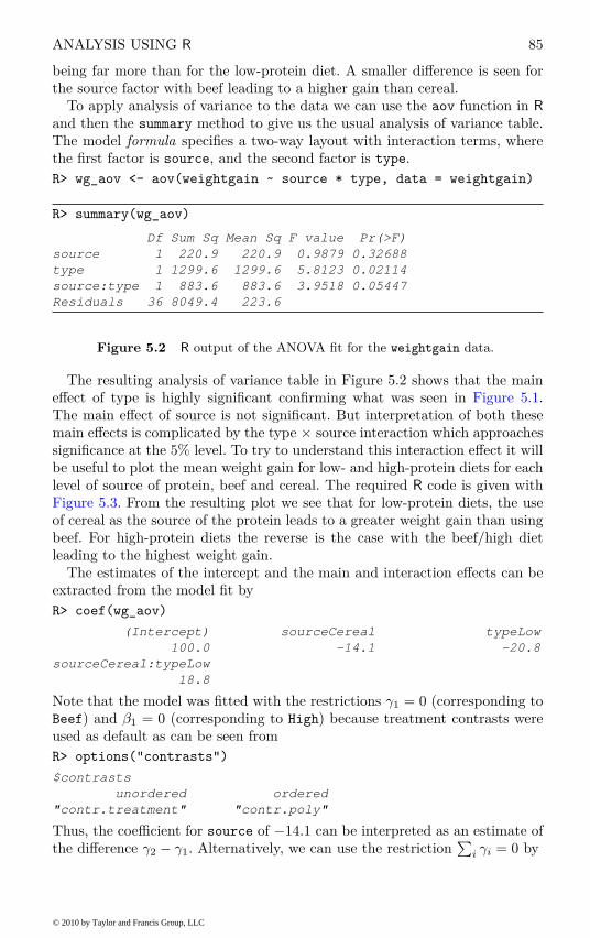
ANALYSIS USING R 85
being far more than for the low-protein diet. A smaller difference is seen forthe source factor with beef leading to a higher gain than cereal.
To apply analysis of variance to the data we can use the aov function in R
and then the summary method to give us the usual analysis of variance table.The model formula specifies a two-way layout with interaction terms, wherethe first factor is source, and the second factor is type.
R> wg_aov <- aov(weightgain ~ source * type, data = weightgain)
R> summary(wg_aov)
Df Sum Sq Mean Sq F value Pr(>F)
source 1 220.9 220.9 0.9879 0.32688
type 1 1299.6 1299.6 5.8123 0.02114
source:type 1 883.6 883.6 3.9518 0.05447
Residuals 36 8049.4 223.6
Figure 5.2 R output of the ANOVA fit for the weightgain data.
The resulting analysis of variance table in Figure 5.2 shows that the maineffect of type is highly significant confirming what was seen in Figure 5.1.The main effect of source is not significant. But interpretation of both thesemain effects is complicated by the type × source interaction which approachessignificance at the 5% level. To try to understand this interaction effect it willbe useful to plot the mean weight gain for low- and high-protein diets for eachlevel of source of protein, beef and cereal. The required R code is given withFigure 5.3. From the resulting plot we see that for low-protein diets, the useof cereal as the source of the protein leads to a greater weight gain than usingbeef. For high-protein diets the reverse is the case with the beef/high dietleading to the highest weight gain.
The estimates of the intercept and the main and interaction effects can beextracted from the model fit by
R> coef(wg_aov)
(Intercept) sourceCereal typeLow
100.0 -14.1 -20.8
sourceCereal:typeLow
18.8
Note that the model was fitted with the restrictions γ1 = 0 (corresponding toBeef) and β1 = 0 (corresponding to High) because treatment contrasts wereused as default as can be seen from
R> options("contrasts")
$contrasts
unordered ordered
"contr.treatment" "contr.poly"
Thus, the coefficient for source of −14.1 can be interpreted as an estimate ofthe difference γ2 − γ1. Alternatively, we can use the restriction
∑
i γi = 0 by
© 2010 by Taylor and Francis Group, LLC
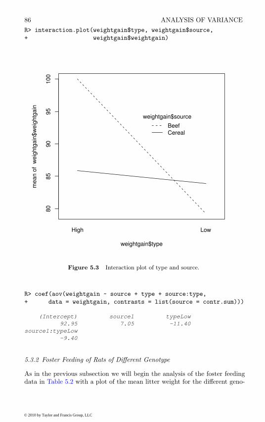
86 ANALYSIS OF VARIANCE
R> interaction.plot(weightgain$type, weightgain$source,
+ weightgain$weightgain)
80
85
90
95
10
0
weightgain$type
me
an
of
we
igh
tga
in$
we
igh
tga
in
High Low
weightgain$source
BeefCereal
Figure 5.3 Interaction plot of type and source.
R> coef(aov(weightgain ~ source + type + source:type,
+ data = weightgain, contrasts = list(source = contr.sum)))
(Intercept) source1 typeLow
92.95 7.05 -11.40
source1:typeLow
-9.40
5.3.2 Foster Feeding of Rats of Different Genotype
As in the previous subsection we will begin the analysis of the foster feedingdata in Table 5.2 with a plot of the mean litter weight for the different geno-
© 2010 by Taylor and Francis Group, LLC
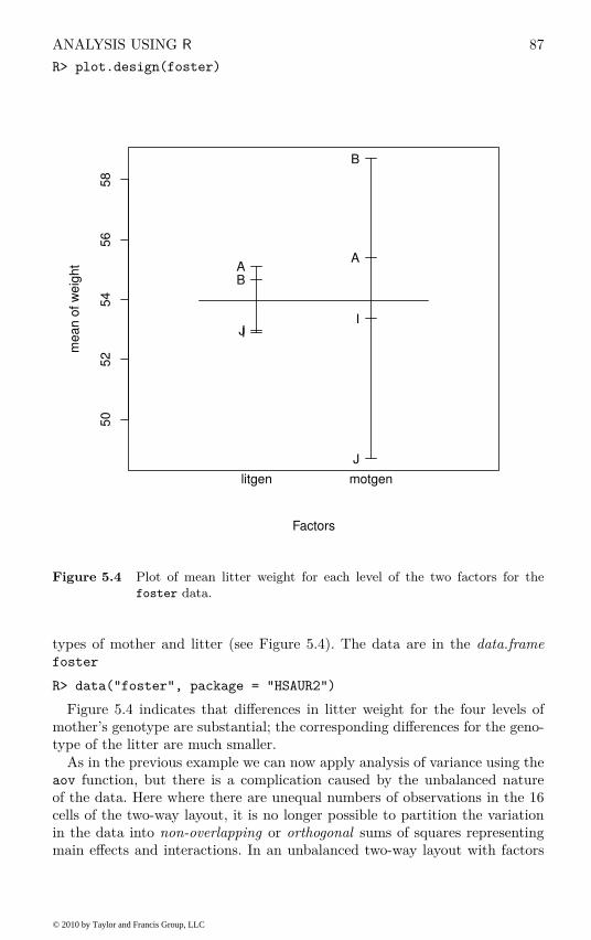
ANALYSIS USING R 87
R> plot.design(foster)
50
52
54
56
58
Factors
me
an
of
we
igh
t AB
IJ
A
B
I
J
litgen motgen
Figure 5.4 Plot of mean litter weight for each level of the two factors for thefoster data.
types of mother and litter (see Figure 5.4). The data are in the data.framefoster
R> data("foster", package = "HSAUR2")
Figure 5.4 indicates that differences in litter weight for the four levels ofmother’s genotype are substantial; the corresponding differences for the geno-type of the litter are much smaller.
As in the previous example we can now apply analysis of variance using theaov function, but there is a complication caused by the unbalanced natureof the data. Here where there are unequal numbers of observations in the 16cells of the two-way layout, it is no longer possible to partition the variationin the data into non-overlapping or orthogonal sums of squares representingmain effects and interactions. In an unbalanced two-way layout with factors
© 2010 by Taylor and Francis Group, LLC

88 ANALYSIS OF VARIANCE
A and B there is a proportion of the variance of the response variable thatcan be attributed to either A or B. The consequence is that A and B togetherexplain less of the variation of the dependent variable than the sum of whicheach explains alone. The result is that the sum of squares corresponding toa factor depends on which other terms are currently in the model for theobservations, so the sums of squares depend on the order in which the factorsare considered and represent a comparison of models. For example, for theorder a, b, a × b, the sums of squares are such that
• SSa: compares the model containing only the a main effect with one con-taining only the overall mean.
• SSb|a: compares the model including both main effects, but no interaction,with one including only the main effect of a.
• SSab|a, b: compares the model including an interaction and main effectswith one including only main effects.
The use of these sums of squares (sometimes known as Type I sums ofsquares) in a series of tables in which the effects are considered in differentorders provides the most appropriate approach to the analysis of unbalanceddesigns.
We can derive the two analyses of variance tables for the foster feedingexample by applying the R code
R> summary(aov(weight ~ litgen * motgen, data = foster))
to give
Df Sum Sq Mean Sq F value Pr(>F)
litgen 3 60.16 20.05 0.3697 0.775221
motgen 3 775.08 258.36 4.7632 0.005736
litgen:motgen 9 824.07 91.56 1.6881 0.120053
Residuals 45 2440.82 54.24
and then the code
R> summary(aov(weight ~ motgen * litgen, data = foster))
to give
Df Sum Sq Mean Sq F value Pr(>F)
motgen 3 771.61 257.20 4.7419 0.005869
litgen 3 63.63 21.21 0.3911 0.760004
motgen:litgen 9 824.07 91.56 1.6881 0.120053
Residuals 45 2440.82 54.24
There are (small) differences in the sum of squares for the two main effectsand, consequently, in the associated F -tests and p-values. This would not betrue if in the previous example in Subsection 5.3.1 we had used the code
R> summary(aov(weightgain ~ type * source, data = weightgain))
instead of the code which produced Figure 5.2 (readers should confirm thatthis is the case).
Although for the foster feeding data the differences in the two analyses ofvariance with different orders of main effects are very small, this may not
© 2010 by Taylor and Francis Group, LLC

ANALYSIS USING R 89
always be the case and care is needed in dealing with unbalanced designs. Fora more complete discussion see Nelder (1977) and Aitkin (1978).
Both ANOVA tables indicate that the main effect of mother’s genotype ishighly significant and that genotype B leads to the greatest litter weight andgenotype J to the smallest litter weight.
We can investigate the effect of genotype B on litter weight in more detail bythe use of multiple comparison procedures (see Everitt, 1996, and Chapter 14).Such procedures allow a comparison of all pairs of levels of a factor whilstmaintaining the nominal significance level at its specified value and producingadjusted confidence intervals for mean differences. One such procedure is calledTukey honest significant differences suggested by Tukey (1953); see Hochbergand Tamhane (1987) also. Here, we are interested in simultaneous confidenceintervals for the weight differences between all four genotypes of the mother.First, an ANOVA model is fitted
R> foster_aov <- aov(weight ~ litgen * motgen, data = foster)
which serves as the basis of the multiple comparisons, here with all pair-wisedifferences by
R> foster_hsd <- TukeyHSD(foster_aov, "motgen")
R> foster_hsd
Tukey multiple comparisons of means
95% family-wise confidence level
Fit: aov(formula = weight ~ litgen * motgen, data = foster)
$motgen
diff lwr upr p adj
B-A 3.330369 -3.859729 10.5204672 0.6078581
I-A -1.895574 -8.841869 5.0507207 0.8853702
J-A -6.566168 -13.627285 0.4949498 0.0767540
I-B -5.225943 -12.416041 1.9641552 0.2266493
J-B -9.896537 -17.197624 -2.5954489 0.0040509
J-I -4.670593 -11.731711 2.3905240 0.3035490
A convenient plot method exists for this object and we can get a graphicalrepresentation of the multiple confidence intervals as shown in Figure 5.5. Itappears that there is only evidence for a difference in the B and J genotypes.Note that the particular method implemented in TukeyHSD is applicable onlyto balanced and mildly unbalanced designs (which is the case here). Alterna-tive approaches, applicable to unbalanced designs and more general researchquestions, will be introduced and discussed in Chapter 14.
5.3.3 Water Hardness and Mortality
The water hardness and mortality data for 61 large towns in England andWales (see Table 3.3) was analysed in Chapter 3 and here we will extend theanalysis by an assessment of the differences of both hardness and mortality
© 2010 by Taylor and Francis Group, LLC
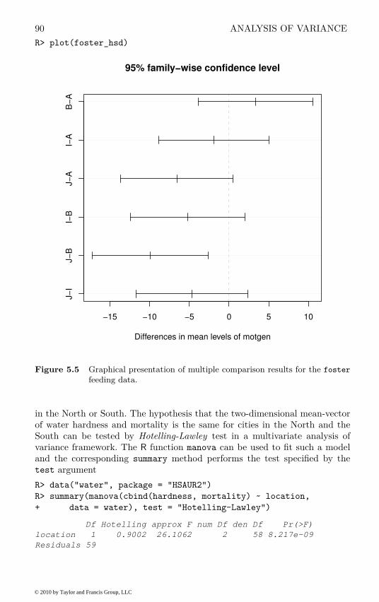
90 ANALYSIS OF VARIANCE
R> plot(foster_hsd)
−15 −10 −5 0 5 10
J−
IJ−
BI−
BJ−
AI−
AB
−A
95% family−wise confidence level
Differences in mean levels of motgen
Figure 5.5 Graphical presentation of multiple comparison results for the foster
feeding data.
in the North or South. The hypothesis that the two-dimensional mean-vectorof water hardness and mortality is the same for cities in the North and theSouth can be tested by Hotelling-Lawley test in a multivariate analysis ofvariance framework. The R function manova can be used to fit such a modeland the corresponding summary method performs the test specified by thetest argument
R> data("water", package = "HSAUR2")
R> summary(manova(cbind(hardness, mortality) ~ location,
+ data = water), test = "Hotelling-Lawley")
Df Hotelling approx F num Df den Df Pr(>F)
location 1 0.9002 26.1062 2 58 8.217e-09
Residuals 59
© 2010 by Taylor and Francis Group, LLC

ANALYSIS USING R 91
The cbind statement in the left hand side of the formula indicates that amultivariate response variable is to be modelled. The p-value associated withthe Hotelling-Lawley statistic is very small and there is strong evidence thatthe mean vectors of the two variables are not the same in the two regions.Looking at the sample means
R> tapply(water$hardness, water$location, mean)
North South
30.40000 69.76923
R> tapply(water$mortality, water$location, mean)
North South
1633.600 1376.808
we see large differences in the two regions both in water hardness and mortal-ity, where low mortality is associated with hard water in the South and highmortality with soft water in the North (see Figure 3.8 also).
5.3.4 Male Egyptian Skulls
We can begin by looking at a table of mean values for the four measure-ments within each of the five epochs. The measurements are available in thedata.frame skulls and we can compute the means over all epochs by
R> data("skulls", package = "HSAUR2")
R> means <- aggregate(skulls[,c("mb", "bh", "bl", "nh")],
+ list(epoch = skulls$epoch), mean)
R> means
epoch mb bh bl nh
1 c4000BC 131.3667 133.6000 99.16667 50.53333
2 c3300BC 132.3667 132.7000 99.06667 50.23333
3 c1850BC 134.4667 133.8000 96.03333 50.56667
4 c200BC 135.5000 132.3000 94.53333 51.96667
5 cAD150 136.1667 130.3333 93.50000 51.36667
It may also be useful to look at these means graphically and this could bedone in a variety of ways. Here we construct a scatterplot matrix of the meansusing the code attached to Figure 5.6.
There appear to be quite large differences between the epoch means, atleast on some of the four measurements. We can now test for a differencemore formally by using MANOVA with the following R code to apply each ofthe four possible test criteria mentioned earlier;
R> skulls_manova <- manova(cbind(mb, bh, bl, nh) ~ epoch,
+ data = skulls)
R> summary(skulls_manova, test = "Pillai")
Df Pillai approx F num Df den Df Pr(>F)
epoch 4 0.3533 3.5120 16 580 4.675e-06
Residuals 145
© 2010 by Taylor and Francis Group, LLC

92 ANALYSIS OF VARIANCE
R> pairs(means[,-1],
+ panel = function(x, y) {
+ text(x, y, abbreviate(levels(skulls$epoch)))
+ })
mb
130.5 132.0 133.5
c400
c330
c185
c200
cAD1
c400
c330
c185
c200
cAD1
50.5 51.5
132
134
136
c400
c330
c185
c200
cAD1
130.5
132.0
133.5
c400
c330
c185
c200
cAD1
bh
c400
c330
c185
c200
cAD1
c400
c330
c185
c200
cAD1
c400c330
c185
c200
cAD1
c400c330
c185
c200
cAD1
bl
94
96
98
c400c330
c185
c200
cAD1
132 134 136
50.5
51.5
c400
c330
c185
c200
cAD1
c400
c330
c185
c200
cAD1
94 96 98
c400
c330
c185
c200
cAD1
nh
Figure 5.6 Scatterplot matrix of epoch means for Egyptian skulls data.
R> summary(skulls_manova, test = "Wilks")
Df Wilks approx F num Df den Df Pr(>F)
epoch 4.00 0.6636 3.9009 16.00 434.45 7.01e-07
Residuals 145.00
R> summary(skulls_manova, test = "Hotelling-Lawley")
Df Hotelling approx F num Df den Df Pr(>F)
epoch 4 0.4818 4.2310 16 562 8.278e-08
Residuals 145
R> summary(skulls_manova, test = "Roy")
© 2010 by Taylor and Francis Group, LLC
ANALYSIS USING R 93
Df Roy approx F num Df den Df Pr(>F)
epoch 4 0.4251 15.4097 4 145 1.588e-10
Residuals 145
The p-value associated with each four test criteria is very small and there isstrong evidence that the skull measurements differ between the five epochs. Wemight now move on to investigate which epochs differ and on which variables.We can look at the univariate F -tests for each of the four variables by usingthe code
R> summary.aov(skulls_manova)
Response mb :
Df Sum Sq Mean Sq F value Pr(>F)
epoch 4 502.83 125.71 5.9546 0.0001826
Residuals 145 3061.07 21.11
Response bh :
Df Sum Sq Mean Sq F value Pr(>F)
epoch 4 229.9 57.5 2.4474 0.04897
Residuals 145 3405.3 23.5
Response bl :
Df Sum Sq Mean Sq F value Pr(>F)
epoch 4 803.3 200.8 8.3057 4.636e-06
Residuals 145 3506.0 24.2
Response nh :
Df Sum Sq Mean Sq F value Pr(>F)
epoch 4 61.20 15.30 1.507 0.2032
Residuals 145 1472.13 10.15
We see that the results for the maximum breadths (mb) and basialiveolar length(bl) are highly significant, with those for the other two variables, in particularfor nasal heights (nh), suggesting little evidence of a difference. To look at thepairwise multivariate tests (any of the four test criteria are equivalent in thecase of a one-way layout with two levels only) we can use the summary methodand manova function as follows:
R> summary(manova(cbind(mb, bh, bl, nh) ~ epoch, data = skulls,
+ subset = epoch %in% c("c4000BC", "c3300BC")))
Df Pillai approx F num Df den Df Pr(>F)
epoch 1 0.02767 0.39135 4 55 0.814
Residuals 58
R> summary(manova(cbind(mb, bh, bl, nh) ~ epoch, data = skulls,
+ subset = epoch %in% c("c4000BC", "c1850BC")))
Df Pillai approx F num Df den Df Pr(>F)
epoch 1 0.1876 3.1744 4 55 0.02035
Residuals 58
© 2010 by Taylor and Francis Group, LLC

94 ANALYSIS OF VARIANCE
R> summary(manova(cbind(mb, bh, bl, nh) ~ epoch, data = skulls,
+ subset = epoch %in% c("c4000BC", "c200BC")))
Df Pillai approx F num Df den Df Pr(>F)
epoch 1 0.3030 5.9766 4 55 0.0004564
Residuals 58
R> summary(manova(cbind(mb, bh, bl, nh) ~ epoch, data = skulls,
+ subset = epoch %in% c("c4000BC", "cAD150")))
Df Pillai approx F num Df den Df Pr(>F)
epoch 1 0.3618 7.7956 4 55 4.736e-05
Residuals 58
To keep the overall significance level for the set of all pairwise multivariatetests under some control (and still maintain a reasonable power), Stevens(2001) recommends setting the nominal level α = 0.15 and carrying out eachtest at the α/m level where m s the number of tests performed. The resultsof the four pairwise tests suggest that as the epochs become further separatedin time the four skull measurements become increasingly distinct.
For more details of applying multiple comparisons in the multivariate situ-ation see Stevens (2001).
5.4 Summary
Analysis of variance is one of the most widely used of statistical techniquesand is easily applied using R as is the extension to multivariate data. Ananalysis of variance needs to be supplemented by graphical material prior toformal analysis and often to more detailed investigation of group differencesusing multiple comparison techniques.
Exercises
Ex. 5.1 Examine the residuals (observed value − fitted value) from fitting amain effects only model to the data in Table 5.1. What conclusions do youdraw?
Ex. 5.2 The data in Table 5.4 below arise from a sociological study of Aus-tralian Aboriginal and white children reported by Quine (1975). In thisstudy, children of both sexes from four age groups (final grade in primaryschools and first, second and third form in secondary school) and from twocultural groups were used. The children in each age group were classifiedas slow or average learners. The response variable was the number of daysabsent from school during the school year. (Children who had suffered aserious illness during the years were excluded.) Carry out what you con-sider to be an appropriate analysis of variance of the data noting that (i)there are unequal numbers of observations in each cell and (ii) the responsevariable here is a count. Interpret your results with the aid of some suitabletables of means and some informative graphs.
© 2010 by Taylor and Francis Group, LLC
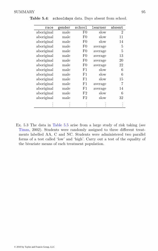
SUMMARY 95
Table 5.4: schooldays data. Days absent from school.
race gender school learner absent
aboriginal male F0 slow 2aboriginal male F0 slow 11aboriginal male F0 slow 14aboriginal male F0 average 5aboriginal male F0 average 5aboriginal male F0 average 13aboriginal male F0 average 20aboriginal male F0 average 22aboriginal male F1 slow 6aboriginal male F1 slow 6aboriginal male F1 slow 15aboriginal male F1 average 7aboriginal male F1 average 14aboriginal male F2 slow 6aboriginal male F2 slow 32
......
......
...
Ex. 5.3 The data in Table 5.5 arise from a large study of risk taking (seeTimm, 2002). Students were randomly assigned to three different treat-ments labelled AA, C and NC. Students were administered two parallelforms of a test called ‘low’ and ‘high’. Carry out a test of the equality ofthe bivariate means of each treatment population.
© 2010 by Taylor and Francis Group, LLC

96 ANALYSIS OF VARIANCE
Table 5.5: students data. Treatment and results of two tests inthree groups of students.
treatment low high treatment low high
AA 8 28 C 34 4AA 18 28 C 34 4AA 8 23 C 44 7AA 12 20 C 39 5AA 15 30 C 20 0AA 12 32 C 43 11AA 18 31 NC 50 5AA 29 25 NC 57 51AA 6 28 NC 62 52AA 7 28 NC 56 52AA 6 24 NC 59 40AA 14 30 NC 61 68AA 11 23 NC 66 49AA 12 20 NC 57 49
C 46 13 NC 62 58C 26 10 NC 47 58C 47 22 NC 53 40C 44 14
Source: From Timm, N. H., Applied Multivariate Analysis, Springer, NewYork, 2002. With kind permission of Springer Science and Business Media.
© 2010 by Taylor and Francis Group, LLC

CHAPTER 6
Simple and Multiple Linear Regression:How Old is the Universe and Cloud
Seeding
6.1 Introduction
Freedman et al. (2001) give the relative velocity and the distance of 24 galaxies,according to measurements made using the Hubble Space Telescope – the dataare contained in the gamair package accompanying Wood (2006), see Table 6.1.Velocities are assessed by measuring the Doppler red shift in the spectrum oflight observed from the galaxies concerned, although some correction for ‘local’velocity components is required. Distances are measured using the knownrelationship between the period of Cepheid variable stars and their luminosity.How can these data be used to estimate the age of the universe? Here we shallshow how this can be done using simple linear regression.
Table 6.1: hubble data. Distance and velocity for 24 galaxies.
galaxy velocity distance galaxy velocity distance
NGC0300 133 2.00 NGC3621 609 6.64NGC0925 664 9.16 NGC4321 1433 15.21
NGC1326A 1794 16.14 NGC4414 619 17.70NGC1365 1594 17.95 NGC4496A 1424 14.86NGC1425 1473 21.88 NGC4548 1384 16.22NGC2403 278 3.22 NGC4535 1444 15.78NGC2541 714 11.22 NGC4536 1423 14.93NGC2090 882 11.75 NGC4639 1403 21.98NGC3031 80 3.63 NGC4725 1103 12.36NGC3198 772 13.80 IC4182 318 4.49NGC3351 642 10.00 NGC5253 232 3.15NGC3368 768 10.52 NGC7331 999 14.72
Source: From Freedman W. L., et al., The Astrophysical Journal, 553, 47–72,2001. With permission.
97
© 2010 by Taylor and Francis Group, LLC

98 SIMPLE AND MULTIPLE LINEAR REGRESSION
Table 6.2: clouds data. Cloud seeding experiments in Florida –see above for explanations of the variables.
seeding time sne cloudcover prewetness echomotion rainfall
no 0 1.75 13.4 0.274 stationary 12.85yes 1 2.70 37.9 1.267 moving 5.52yes 3 4.10 3.9 0.198 stationary 6.29no 4 2.35 5.3 0.526 moving 6.11
yes 6 4.25 7.1 0.250 moving 2.45no 9 1.60 6.9 0.018 stationary 3.61no 18 1.30 4.6 0.307 moving 0.47no 25 3.35 4.9 0.194 moving 4.56no 27 2.85 12.1 0.751 moving 6.35
yes 28 2.20 5.2 0.084 moving 5.06yes 29 4.40 4.1 0.236 moving 2.76yes 32 3.10 2.8 0.214 moving 4.05no 33 3.95 6.8 0.796 moving 5.74
yes 35 2.90 3.0 0.124 moving 4.84yes 38 2.05 7.0 0.144 moving 11.86no 39 4.00 11.3 0.398 moving 4.45no 53 3.35 4.2 0.237 stationary 3.66
yes 55 3.70 3.3 0.960 moving 4.22no 56 3.80 2.2 0.230 moving 1.16
yes 59 3.40 6.5 0.142 stationary 5.45yes 65 3.15 3.1 0.073 moving 2.02no 68 3.15 2.6 0.136 moving 0.82
yes 82 4.01 8.3 0.123 moving 1.09no 83 4.65 7.4 0.168 moving 0.28
Weather modification, or cloud seeding, is the treatment of individual cloudsor storm systems with various inorganic and organic materials in the hope ofachieving an increase in rainfall. Introduction of such material into a cloudthat contains supercooled water, that is, liquid water colder than zero degreesof Celsius, has the aim of inducing freezing, with the consequent ice particlesgrowing at the expense of liquid droplets and becoming heavy enough to fallas rain from clouds that otherwise would produce none.
The data shown in Table 6.2 were collected in the summer of 1975 from anexperiment to investigate the use of massive amounts of silver iodide (100 to1000 grams per cloud) in cloud seeding to increase rainfall (Woodley et al.,1977). In the experiment, which was conducted in an area of Florida, 24 dayswere judged suitable for seeding on the basis that a measured suitability cri-terion, denoted S-Ne, was not less than 1.5. Here S is the ‘seedability’, thedifference between the maximum height of a cloud if seeded and the same cloudif not seeded predicted by a suitable cloud model, and Ne is the number of
© 2010 by Taylor and Francis Group, LLC
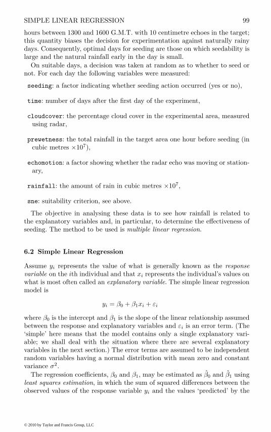
SIMPLE LINEAR REGRESSION 99
hours between 1300 and 1600 G.M.T. with 10 centimetre echoes in the target;this quantity biases the decision for experimentation against naturally rainydays. Consequently, optimal days for seeding are those on which seedability islarge and the natural rainfall early in the day is small.
On suitable days, a decision was taken at random as to whether to seed ornot. For each day the following variables were measured:
seeding: a factor indicating whether seeding action occurred (yes or no),
time: number of days after the first day of the experiment,
cloudcover: the percentage cloud cover in the experimental area, measuredusing radar,
prewetness: the total rainfall in the target area one hour before seeding (incubic metres ×107),
echomotion: a factor showing whether the radar echo was moving or station-ary,
rainfall: the amount of rain in cubic metres ×107,
sne: suitability criterion, see above.
The objective in analysing these data is to see how rainfall is related tothe explanatory variables and, in particular, to determine the effectiveness ofseeding. The method to be used is multiple linear regression.
6.2 Simple Linear Regression
Assume yi represents the value of what is generally known as the response
variable on the ith individual and that xi represents the individual’s values onwhat is most often called an explanatory variable. The simple linear regressionmodel is
yi = β0 + β1xi + εi
where β0 is the intercept and β1 is the slope of the linear relationship assumedbetween the response and explanatory variables and εi is an error term. (The‘simple’ here means that the model contains only a single explanatory vari-able; we shall deal with the situation where there are several explanatoryvariables in the next section.) The error terms are assumed to be independentrandom variables having a normal distribution with mean zero and constantvariance σ2.
The regression coefficients, β0 and β1, may be estimated as β0 and β1 usingleast squares estimation, in which the sum of squared differences between theobserved values of the response variable yi and the values ‘predicted’ by the
© 2010 by Taylor and Francis Group, LLC
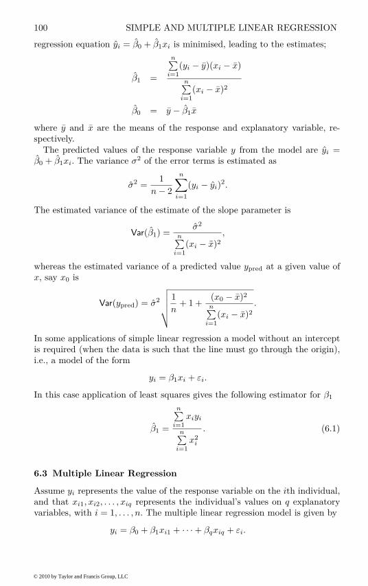
100 SIMPLE AND MULTIPLE LINEAR REGRESSION
regression equation yi = β0 + β1xi is minimised, leading to the estimates;
β1 =
n∑
i=1
(yi − y)(xi − x)
n∑
i=1
(xi − x)2
β0 = y − β1x
where y and x are the means of the response and explanatory variable, re-spectively.
The predicted values of the response variable y from the model are yi =β0 + β1xi. The variance σ2 of the error terms is estimated as
σ2 =1
n − 2
n∑
i=1
(yi − yi)2.
The estimated variance of the estimate of the slope parameter is
Var(β1) =σ2
n∑
i=1
(xi − x)2
,
whereas the estimated variance of a predicted value ypred at a given value ofx, say x0 is
Var(ypred) = σ2
√
√
√
√
√
1
n+ 1 +
(x0 − x)2
n∑
i=1
(xi − x)2
.
In some applications of simple linear regression a model without an interceptis required (when the data is such that the line must go through the origin),i.e., a model of the form
yi = β1xi + εi.
In this case application of least squares gives the following estimator for β1
β1 =
n∑
i=1
xiyi
n∑
i=1
x2i
. (6.1)
6.3 Multiple Linear Regression
Assume yi represents the value of the response variable on the ith individual,and that xi1, xi2, . . . , xiq represents the individual’s values on q explanatoryvariables, with i = 1, . . . , n. The multiple linear regression model is given by
yi = β0 + β1xi1 + · · · + βqxiq + εi.
© 2010 by Taylor and Francis Group, LLC

MULTIPLE LINEAR REGRESSION 101
The error terms εi, i = 1, . . . , n, are assumed to be independent randomvariables having a normal distribution with mean zero and constant varianceσ2. Consequently, the distribution of the random response variable, y, is alsonormal with expected value given by the linear combination of the explanatoryvariables
E(y|x1, . . . , xq) = β0 + β1x1 + · · · + βqxq
and with variance σ2.The parameters of the model βk, k = 1, . . . , q, are known as regression
coefficients with β0 corresponding to the overall mean. The regression coeffi-cients represent the expected change in the response variable associated witha unit change in the corresponding explanatory variable, when the remainingexplanatory variables are held constant. The linear in multiple linear regres-sion applies to the regression parameters, not to the response or explanatoryvariables. Consequently, models in which, for example, the logarithm of a re-sponse variable is modelled in terms of quadratic functions of some of theexplanatory variables would be included in this class of models.
The multiple linear regression model can be written most conveniently forall n individuals by using matrices and vectors as y = Xβ + ε where y⊤ =(y1, . . . , yn) is the vector of response variables, β⊤ = (β0, β1, . . . , βq) is thevector of regression coefficients, and ε⊤ = (ε1, . . . , εn) are the error terms. Thedesign or model matrix X consists of the q continuously measured explanatoryvariables and a column of ones corresponding to the intercept term
X =
1 x11 x12 . . . x1q
1 x21 x22 . . . x2q
......
.... . .
...1 xn1 xn2 . . . xnq
.
In case one or more of the explanatory variables are nominal or ordinal vari-ables, they are represented by a zero-one dummy coding. Assume that x1 is afactor at m levels, the submatrix of X corresponding to x1 is a n×m matrixof zeros and ones, where the jth element in the ith row is one when xi1 is atthe jth level.
Assuming that the cross-product X⊤X is non-singular, i.e., can be inverted,then the least squares estimator of the parameter vector β is unique and canbe calculated by β = (X⊤X)−1X⊤y. The expectation and covariance of this
estimator β are given by E(β) = β and Var(β) = σ2(X⊤X)−1. The diagonal
elements of the covariance matrix Var(β) give the variances of βj , j = 0, . . . , q,
whereas the off diagonal elements give the covariances between pairs of βj
and βk. The square roots of the diagonal elements of the covariance matrixare thus the standard errors of the estimates βj .
If the cross-product X⊤X is singular we need to reformulate the model toy = XCβ⋆ + ε such that X⋆ = XC has full rank. The matrix C is called thecontrast matrix in S and R and the result of the model fit is an estimate β⋆.
© 2010 by Taylor and Francis Group, LLC
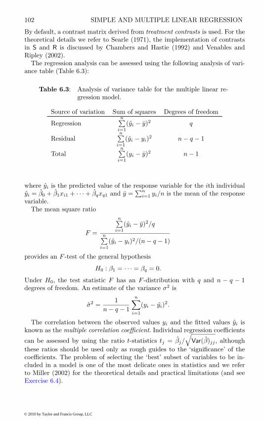
102 SIMPLE AND MULTIPLE LINEAR REGRESSION
By default, a contrast matrix derived from treatment contrasts is used. For thetheoretical details we refer to Searle (1971), the implementation of contrastsin S and R is discussed by Chambers and Hastie (1992) and Venables andRipley (2002).
The regression analysis can be assessed using the following analysis of vari-ance table (Table 6.3):
Table 6.3: Analysis of variance table for the multiple linear re-gression model.
Source of variation Sum of squares Degrees of freedom
Regressionn∑
i=1
(yi − y)2 q
Residualn∑
i=1
(yi − yi)2 n − q − 1
Totaln∑
i=1
(yi − y)2 n − 1
where yi is the predicted value of the response variable for the ith individualyi = β0 + β1xi1 + · · · + βqxq1 and y =
∑n
i=1 yi/n is the mean of the responsevariable.
The mean square ratio
F =
n∑
i=1
(yi − y)2/q
n∑
i=1
(yi − yi)2/(n − q − 1)
provides an F -test of the general hypothesis
H0 : β1 = · · · = βq = 0.
Under H0, the test statistic F has an F -distribution with q and n − q − 1degrees of freedom. An estimate of the variance σ2 is
σ2 =1
n − q − 1
n∑
i=1
(yi − yi)2.
The correlation between the observed values yi and the fitted values yi isknown as the multiple correlation coefficient. Individual regression coefficients
can be assessed by using the ratio t-statistics tj = βj/
√
Var(β)jj , although
these ratios should be used only as rough guides to the ‘significance’ of thecoefficients. The problem of selecting the ‘best’ subset of variables to be in-cluded in a model is one of the most delicate ones in statistics and we referto Miller (2002) for the theoretical details and practical limitations (and seeExercise 6.4).
© 2010 by Taylor and Francis Group, LLC
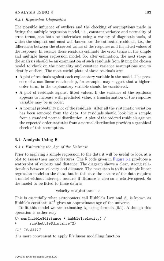
ANALYSIS USING R 103
6.3.1 Regression Diagnostics
The possible influence of outliers and the checking of assumptions made infitting the multiple regression model, i.e., constant variance and normality oferror terms, can both be undertaken using a variety of diagnostic tools, ofwhich the simplest and most well known are the estimated residuals, i.e., thedifferences between the observed values of the response and the fitted values ofthe response. In essence these residuals estimate the error terms in the simpleand multiple linear regression model. So, after estimation, the next stage inthe analysis should be an examination of such residuals from fitting the chosenmodel to check on the normality and constant variance assumptions and toidentify outliers. The most useful plots of these residuals are:
• A plot of residuals against each explanatory variable in the model. The pres-ence of a non-linear relationship, for example, may suggest that a higher-order term, in the explanatory variable should be considered.
• A plot of residuals against fitted values. If the variance of the residualsappears to increase with predicted value, a transformation of the responsevariable may be in order.
• A normal probability plot of the residuals. After all the systematic variationhas been removed from the data, the residuals should look like a samplefrom a standard normal distribution. A plot of the ordered residuals againstthe expected order statistics from a normal distribution provides a graphicalcheck of this assumption.
6.4 Analysis Using R
6.4.1 Estimating the Age of the Universe
Prior to applying a simple regression to the data it will be useful to look at aplot to assess their major features. The R code given in Figure 6.1 produces ascatterplot of velocity and distance. The diagram shows a clear, strong rela-tionship between velocity and distance. The next step is to fit a simple linearregression model to the data, but in this case the nature of the data requiresa model without intercept because if distance is zero so is relative speed. Sothe model to be fitted to these data is
velocity = β1distance + ε.
This is essentially what astronomers call Hubble’s Law and β1 is known asHubble’s constant; β−1
1 gives an approximate age of the universe.To fit this model we are estimating β1 using formula (6.1). Although this
operation is rather easy
R> sum(hubble$distance * hubble$velocity) /
+ sum(hubble$distance^2)
[1] 76.58117
it is more convenient to apply R’s linear modelling function
© 2010 by Taylor and Francis Group, LLC

104 SIMPLE AND MULTIPLE LINEAR REGRESSION
R> plot(velocity ~ distance, data = hubble)
5 10 15 20
50
01
00
01
50
0
distance
velo
city
Figure 6.1 Scatterplot of velocity and distance.
R> hmod <- lm(velocity ~ distance - 1, data = hubble)
Note that the model formula specifies a model without intercept. We can nowextract the estimated model coefficients via
R> coef(hmod)
distance
76.58117
and add this estimated regression line to the scatterplot; the result is shownin Figure 6.2. In addition, we produce a scatterplot of the residuals yi −
yi against fitted values yi to assess the quality of the model fit. It seemsthat for higher distance values the variance of velocity increases; however, weare interested in only the estimated parameter β1 which remains valid undervariance heterogeneity (in contrast to t-tests and associated p-values).
Now we can use the estimated value of β1 to find an approximate value
© 2010 by Taylor and Francis Group, LLC
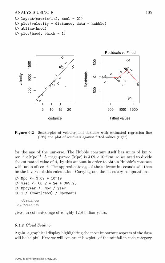
ANALYSIS USING R 105
R> layout(matrix(1:2, ncol = 2))
R> plot(velocity ~ distance, data = hubble)
R> abline(hmod)
R> plot(hmod, which = 1)
5 10 15 20
50
01
00
01
50
0
distance
velo
city
500 1000 1500
−5
00
05
00
Fitted values
Re
sid
ua
ls
Residuals vs Fitted
15
3
16
Figure 6.2 Scatterplot of velocity and distance with estimated regression line(left) and plot of residuals against fitted values (right).
for the age of the universe. The Hubble constant itself has units of km ×
sec−1× Mpc−1. A mega-parsec (Mpc) is 3.09 × 10¹⁹km, so we need to divide
the estimated value of β1 by this amount in order to obtain Hubble’s constantwith units of sec−1. The approximate age of the universe in seconds will thenbe the inverse of this calculation. Carrying out the necessary computations
R> Mpc <- 3.09 * 10^19
R> ysec <- 60^2 * 24 * 365.25
R> Mpcyear <- Mpc / ysec
R> 1 / (coef(hmod) / Mpcyear)
distance
12785935335
gives an estimated age of roughly 12.8 billion years.
6.4.2 Cloud Seeding
Again, a graphical display highlighting the most important aspects of the datawill be helpful. Here we will construct boxplots of the rainfall in each category
© 2010 by Taylor and Francis Group, LLC

106 SIMPLE AND MULTIPLE LINEAR REGRESSION
of the dichotomous explanatory variables and scatterplots of rainfall againsteach of the continuous explanatory variables.
Both the boxplots (Figure 6.3) and the scatterplots (Figure 6.4) show someevidence of outliers. The row names of the extreme observations in the clouds
data.frame can be identified via
R> rownames(clouds)[clouds$rainfall %in% c(bxpseeding$out,
+ bxpecho$out)]
[1] "1" "15"
where bxpseeding and bxpecho are variables created by boxplot in Fig-ure 6.3. Now we shall not remove these observations but bear in mind duringthe modelling process that they may cause problems.
In this example it is sensible to assume that the effect that some of theother explanatory variables is modified by seeding and therefore consider amodel that includes seeding as covariate and, furthermore, allows interactionterms for seeding with each of the covariates except time. This model canbe described by the formula
R> clouds_formula <- rainfall ~ seeding +
+ seeding:(sne + cloudcover + prewetness + echomotion) +
+ time
and the design matrix X⋆ can be computed via
R> Xstar <- model.matrix(clouds_formula, data = clouds)
By default, treatment contrasts have been applied to the dummy codings ofthe factors seeding and echomotion as can be seen from the inspection ofthe contrasts attribute of the model matrix
R> attr(Xstar, "contrasts")
$seeding
[1] "contr.treatment"
$echomotion
[1] "contr.treatment"
The default contrasts can be changed via the contrasts.arg argument tomodel.matrix or the contrasts argument to the fitting function, for examplelm or aov as shown in Chapter 5.
However, such internals are hidden and performed by high-level model-fitting functions such as lm which will be used to fit the linear model definedby the formula clouds_formula:
R> clouds_lm <- lm(clouds_formula, data = clouds)
R> class(clouds_lm)
[1] "lm"
The results of the model fitting is an object of class lm for which a summary
method showing the conventional regression analysis output is available. The
© 2010 by Taylor and Francis Group, LLC
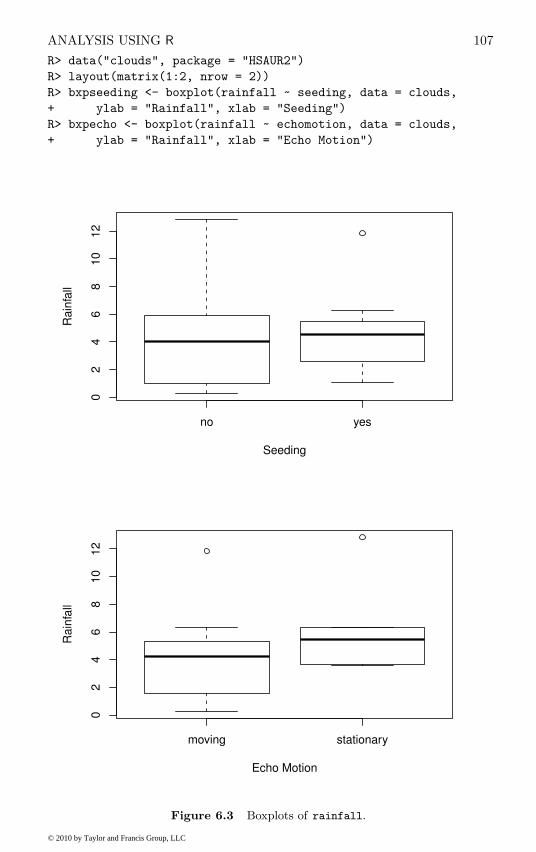
ANALYSIS USING R 107
R> data("clouds", package = "HSAUR2")
R> layout(matrix(1:2, nrow = 2))
R> bxpseeding <- boxplot(rainfall ~ seeding, data = clouds,
+ ylab = "Rainfall", xlab = "Seeding")
R> bxpecho <- boxplot(rainfall ~ echomotion, data = clouds,
+ ylab = "Rainfall", xlab = "Echo Motion")
no yes
02
46
81
01
2
Seeding
Ra
infa
ll
moving stationary
02
46
81
01
2
Echo Motion
Ra
infa
ll
Figure 6.3 Boxplots of rainfall.
© 2010 by Taylor and Francis Group, LLC

108 SIMPLE AND MULTIPLE LINEAR REGRESSION
R> layout(matrix(1:4, nrow = 2))
R> plot(rainfall ~ time, data = clouds)
R> plot(rainfall ~ cloudcover, data = clouds)
R> plot(rainfall ~ sne, data = clouds, xlab="S-Ne criterion")
R> plot(rainfall ~ prewetness, data = clouds)
0 20 40 60 80
02
46
81
01
2
time
rain
fall
5 10 15 20 25 30 35
02
46
81
01
2
cloudcover
rain
fall
1.5 2.0 2.5 3.0 3.5 4.0 4.5
02
46
81
01
2
S−Ne criterion
rain
fall
0.0 0.2 0.4 0.6 0.8 1.0 1.2
02
46
81
01
2
prewetness
rain
fall
Figure 6.4 Scatterplots of rainfall against the continuous covariates.
output in Figure 6.5 shows the estimates β⋆ with corresponding standarderrors and t-statistics as well as the F -statistic with associated p-value.
Many methods are available for extracting components of the fitted model.The estimates β⋆ can be assessed via
R> betastar <- coef(clouds_lm)
R> betastar
(Intercept)
-0.34624093
seedingyes
© 2010 by Taylor and Francis Group, LLC

ANALYSIS USING R 109
R> summary(clouds_lm)
Call:
lm(formula = clouds_formula, data = clouds)
Residuals:
Min 1Q Median 3Q Max
-2.5259 -1.1486 -0.2704 1.0401 4.3913
Coefficients:
Estimate Std. Error t value
(Intercept) -0.34624 2.78773 -0.124
seedingyes 15.68293 4.44627 3.527
time -0.04497 0.02505 -1.795
seedingno:sne 0.41981 0.84453 0.497
seedingyes:sne -2.77738 0.92837 -2.992
seedingno:cloudcover 0.38786 0.21786 1.780
seedingyes:cloudcover -0.09839 0.11029 -0.892
seedingno:prewetness 4.10834 3.60101 1.141
seedingyes:prewetness 1.55127 2.69287 0.576
seedingno:echomotionstationary 3.15281 1.93253 1.631
seedingyes:echomotionstationary 2.59060 1.81726 1.426
Pr(>|t|)
(Intercept) 0.90306
seedingyes 0.00372
time 0.09590
seedingno:sne 0.62742
seedingyes:sne 0.01040
seedingno:cloudcover 0.09839
seedingyes:cloudcover 0.38854
seedingno:prewetness 0.27450
seedingyes:prewetness 0.57441
seedingno:echomotionstationary 0.12677
seedingyes:echomotionstationary 0.17757
Residual standard error: 2.205 on 13 degrees of freedom
Multiple R-squared: 0.7158, Adjusted R-squared: 0.4972
F-statistic: 3.274 on 10 and 13 DF, p-value: 0.02431
Figure 6.5 R output of the linear model fit for the clouds data.
15.68293481
time
-0.04497427
seedingno:sne
0.41981393
seedingyes:sne
-2.77737613
© 2010 by Taylor and Francis Group, LLC

110 SIMPLE AND MULTIPLE LINEAR REGRESSION
seedingno:cloudcover
0.38786207
seedingyes:cloudcover
-0.09839285
seedingno:prewetness
4.10834188
seedingyes:prewetness
1.55127493
seedingno:echomotionstationary
3.15281358
seedingyes:echomotionstationary
2.59059513
and the corresponding covariance matrix Cov(β⋆) is available from the vcov
method
R> Vbetastar <- vcov(clouds_lm)
where the square roots of the diagonal elements are the standard errors asshown in Figure 6.5
R> sqrt(diag(Vbetastar))
(Intercept)
2.78773403
seedingyes
4.44626606
time
0.02505286
seedingno:sne
0.84452994
seedingyes:sne
0.92837010
seedingno:cloudcover
0.21785501
seedingyes:cloudcover
0.11028981
seedingno:prewetness
3.60100694
seedingyes:prewetness
2.69287308
seedingno:echomotionstationary
1.93252592
seedingyes:echomotionstationary
1.81725973
The results of the linear model fit, as shown in Figure 6.5, suggests thatrainfall can be increased by cloud seeding. Moreover, the model indicates thathigher values of the S-Ne criterion lead to less rainfall, but only on days whencloud seeding happened, i.e., the interaction of seeding with S-Ne significantlyaffects rainfall. A suitable graph will help in the interpretation of this result.We can plot the relationship between rainfall and S-Ne for seeding and non-seeding days using the R code shown with Figure 6.6.
© 2010 by Taylor and Francis Group, LLC

ANALYSIS USING R 111
R> psymb <- as.numeric(clouds$seeding)
R> plot(rainfall ~ sne, data = clouds, pch = psymb,
+ xlab = "S-Ne criterion")
R> abline(lm(rainfall ~ sne, data = clouds,
+ subset = seeding == "no"))
R> abline(lm(rainfall ~ sne, data = clouds,
+ subset = seeding == "yes"), lty = 2)
R> legend("topright", legend = c("No seeding", "Seeding"),
+ pch = 1:2, lty = 1:2, bty = "n")
1.5 2.0 2.5 3.0 3.5 4.0 4.5
02
46
81
01
2
S−Ne criterion
rain
fall
No seedingSeeding
Figure 6.6 Regression relationship between S-Ne criterion and rainfall with andwithout seeding.
© 2010 by Taylor and Francis Group, LLC
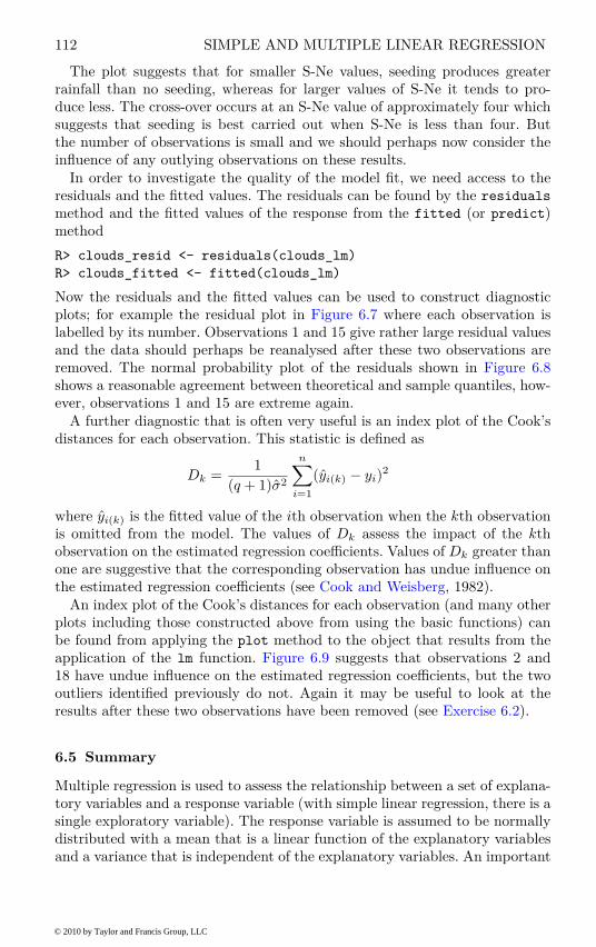
112 SIMPLE AND MULTIPLE LINEAR REGRESSION
The plot suggests that for smaller S-Ne values, seeding produces greaterrainfall than no seeding, whereas for larger values of S-Ne it tends to pro-duce less. The cross-over occurs at an S-Ne value of approximately four whichsuggests that seeding is best carried out when S-Ne is less than four. Butthe number of observations is small and we should perhaps now consider theinfluence of any outlying observations on these results.
In order to investigate the quality of the model fit, we need access to theresiduals and the fitted values. The residuals can be found by the residuals
method and the fitted values of the response from the fitted (or predict)method
R> clouds_resid <- residuals(clouds_lm)
R> clouds_fitted <- fitted(clouds_lm)
Now the residuals and the fitted values can be used to construct diagnosticplots; for example the residual plot in Figure 6.7 where each observation islabelled by its number. Observations 1 and 15 give rather large residual valuesand the data should perhaps be reanalysed after these two observations areremoved. The normal probability plot of the residuals shown in Figure 6.8shows a reasonable agreement between theoretical and sample quantiles, how-ever, observations 1 and 15 are extreme again.
A further diagnostic that is often very useful is an index plot of the Cook’sdistances for each observation. This statistic is defined as
Dk =1
(q + 1)σ2
n∑
i=1
(yi(k) − yi)2
where yi(k) is the fitted value of the ith observation when the kth observationis omitted from the model. The values of Dk assess the impact of the kthobservation on the estimated regression coefficients. Values of Dk greater thanone are suggestive that the corresponding observation has undue influence onthe estimated regression coefficients (see Cook and Weisberg, 1982).
An index plot of the Cook’s distances for each observation (and many otherplots including those constructed above from using the basic functions) canbe found from applying the plot method to the object that results from theapplication of the lm function. Figure 6.9 suggests that observations 2 and18 have undue influence on the estimated regression coefficients, but the twooutliers identified previously do not. Again it may be useful to look at theresults after these two observations have been removed (see Exercise 6.2).
6.5 Summary
Multiple regression is used to assess the relationship between a set of explana-tory variables and a response variable (with simple linear regression, there is asingle exploratory variable). The response variable is assumed to be normallydistributed with a mean that is a linear function of the explanatory variablesand a variance that is independent of the explanatory variables. An important
© 2010 by Taylor and Francis Group, LLC
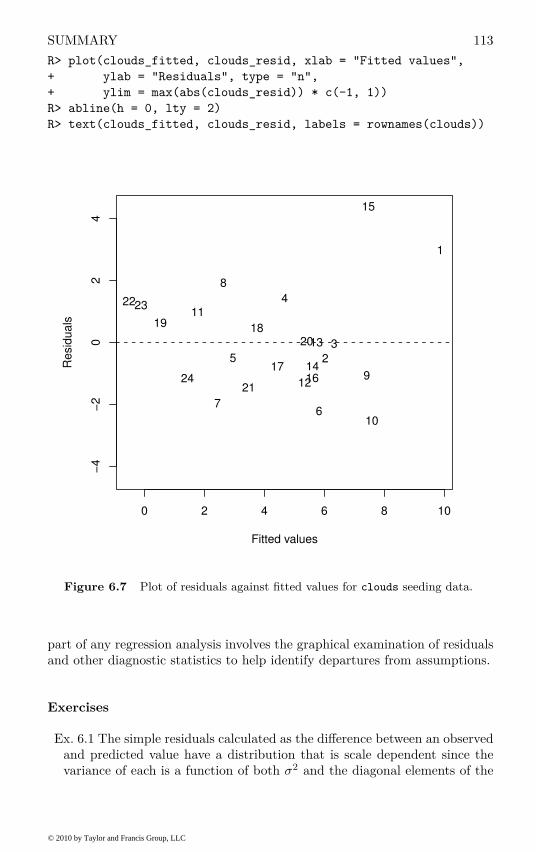
SUMMARY 113
R> plot(clouds_fitted, clouds_resid, xlab = "Fitted values",
+ ylab = "Residuals", type = "n",
+ ylim = max(abs(clouds_resid)) * c(-1, 1))
R> abline(h = 0, lty = 2)
R> text(clouds_fitted, clouds_resid, labels = rownames(clouds))
0 2 4 6 8 10
−4
−2
02
4
Fitted values
Re
sid
ua
ls
1
2
3
4
5
67
8
9
10
11
12
13
14
15
1617
1819
20
21
2223
24
Figure 6.7 Plot of residuals against fitted values for clouds seeding data.
part of any regression analysis involves the graphical examination of residualsand other diagnostic statistics to help identify departures from assumptions.
Exercises
Ex. 6.1 The simple residuals calculated as the difference between an observedand predicted value have a distribution that is scale dependent since thevariance of each is a function of both σ2 and the diagonal elements of the
© 2010 by Taylor and Francis Group, LLC

114 SIMPLE AND MULTIPLE LINEAR REGRESSION
R> qqnorm(clouds_resid, ylab = "Residuals")
R> qqline(clouds_resid)
−2 −1 0 1 2
−2
−1
01
23
4
Normal Q−Q Plot
Theoretical Quantiles
Re
sid
ua
ls
Figure 6.8 Normal probability plot of residuals from cloud seeding modelclouds_lm.
hat matrix H given by
H = X(X⊤X)−1X⊤.
Consequently it is often more useful to work with the standardised versionof the residuals that does not depend on either of these quantities. Thesestandardised residuals are calculated as
ri =yi − yi
σ√
1 − hii
where σ2 is the estimator of σ2 and hii is the ith diagonal element of H.Write an R function to calculate these residuals and use it to obtain some
© 2010 by Taylor and Francis Group, LLC
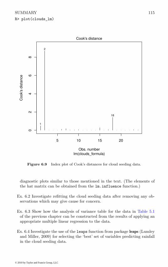
SUMMARY 115
R> plot(clouds_lm)
5 10 15 20
02
46
8
Obs. number
Co
ok's
dis
tan
ce
lm(clouds_formula)
Cook's distance
2
18
1
Figure 6.9 Index plot of Cook’s distances for cloud seeding data.
diagnostic plots similar to those mentioned in the text. (The elements ofthe hat matrix can be obtained from the lm.influence function.)
Ex. 6.2 Investigate refitting the cloud seeding data after removing any ob-servations which may give cause for concern.
Ex. 6.3 Show how the analysis of variance table for the data in Table 5.1of the previous chapter can be constructed from the results of applying anappropriate multiple linear regression to the data.
Ex. 6.4 Investigate the use of the leaps function from package leaps (Lumleyand Miller, 2009) for selecting the ‘best’ set of variables predicting rainfallin the cloud seeding data.
© 2010 by Taylor and Francis Group, LLC

116 SIMPLE AND MULTIPLE LINEAR REGRESSION
Ex. 6.5 Remove the observations for galaxies having leverage greater than0.08 and refit the zero intercept model. What is the estimated age of theuniverse from this model?
Ex. 6.6 Fit a quadratic regression model, i.e, a model of the form
velocity = β1 × distance + β2 × distance2 + ε,
to the hubble data and plot the fitted curve and the simple linear regressionfit on a scatterplot of the data. Which model do you consider most sensibleconsidering the nature of the data? (The ‘quadratic model’ here is stillregarded as a linear regression model since the term linear relates to theparameters of the model not to the powers of the explanatory variable.)
© 2010 by Taylor and Francis Group, LLC

CHAPTER 7
Logistic Regression and GeneralisedLinear Models: Blood Screening,Women’s Role in Society, Colonic
Polyps, and Driving and Back Pain
7.1 Introduction
The erythrocyte sedimentation rate (ESR) is the rate at which red blood cells(erythrocytes) settle out of suspension in blood plasma, when measured understandard conditions. If the ESR increases when the level of certain proteinsin the blood plasma rise in association with conditions such as rheumaticdiseases, chronic infections and malignant diseases, its determination might beuseful in screening blood samples taken from people suspected of suffering fromone of the conditions mentioned. The absolute value of the ESR is not of greatimportance; rather, less than 20mm/hr indicates a ‘healthy’ individual. Toassess whether the ESR is a useful diagnostic tool, Collett and Jemain (1985)collected the data shown in Table 7.1. The question of interest is whetherthere is any association between the probability of an ESR reading greaterthan 20mm/hr and the levels of the two plasma proteins. If there is not thenthe determination of ESR would not be useful for diagnostic purposes.
Table 7.1: plasma data. Blood plasma data.
fibrinogen globulin ESR fibrinogen globulin ESR
2.52 38 ESR < 20 2.88 30 ESR < 202.56 31 ESR < 20 2.65 46 ESR < 202.19 33 ESR < 20 2.28 36 ESR < 202.18 31 ESR < 20 2.67 39 ESR < 203.41 37 ESR < 20 2.29 31 ESR < 202.46 36 ESR < 20 2.15 31 ESR < 203.22 38 ESR < 20 2.54 28 ESR < 202.21 37 ESR < 20 3.34 30 ESR < 203.15 39 ESR < 20 2.99 36 ESR < 202.60 41 ESR < 20 3.32 35 ESR < 202.29 36 ESR < 20 5.06 37 ESR > 202.35 29 ESR < 20 3.34 32 ESR > 203.15 36 ESR < 20 2.38 37 ESR > 202.68 34 ESR < 20 3.53 46 ESR > 20
117
© 2010 by Taylor and Francis Group, LLC
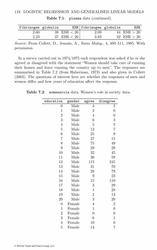
118 LOGISTIC REGRESSION AND GENERALISED LINEAR MODELS
Table 7.1: plasma data (continued).
fibrinogen globulin ESR fibrinogen globulin ESR
2.60 38 ESR < 20 2.09 44 ESR > 202.23 37 ESR < 20 3.93 32 ESR > 20
Source: From Collett, D., Jemain, A., Sains Malay., 4, 493–511, 1985. Withpermission.
In a survey carried out in 1974/1975 each respondent was asked if he or sheagreed or disagreed with the statement “Women should take care of runningtheir homes and leave running the country up to men”. The responses aresummarised in Table 7.2 (from Haberman, 1973) and also given in Collett(2003). The questions of interest here are whether the responses of men andwomen differ and how years of education affect the response.
Table 7.2: womensrole data. Women’s role in society data.
education gender agree disagree
0 Male 4 21 Male 2 02 Male 4 03 Male 6 34 Male 5 55 Male 13 76 Male 25 97 Male 27 158 Male 75 499 Male 29 29
10 Male 32 4511 Male 36 5912 Male 115 24513 Male 31 7014 Male 28 7915 Male 9 2316 Male 15 11017 Male 3 2918 Male 1 2819 Male 2 1320 Male 3 200 Female 4 21 Female 1 02 Female 0 03 Female 6 14 Female 10 05 Female 14 7
© 2010 by Taylor and Francis Group, LLC

INTRODUCTION 119
Table 7.2: womensrole data (continued).
education gender agree disagree
6 Female 17 57 Female 26 168 Female 91 369 Female 30 35
10 Female 55 6711 Female 50 6212 Female 190 40313 Female 17 9214 Female 18 8115 Female 7 3416 Female 13 11517 Female 3 2818 Female 0 2119 Female 1 220 Female 2 4
Source: From Haberman, S. J., Biometrics, 29, 205–220, 1973. With permis-sion.
Giardiello et al. (1993) and Piantadosi (1997) describe the results of aplacebo-controlled trial of a non-steroidal anti-inflammatory drug in the treat-ment of familial andenomatous polyposis (FAP). The trial was halted after aplanned interim analysis had suggested compelling evidence in favour of thetreatment. The data shown in Table 7.3 give the number of colonic polypsafter a 12-month treatment period. The question of interest is whether thenumber of polyps is related to treatment and/or age of patients.
Table 7.3: polyps data. Number of polyps for two treatmentarms.
number treat age number treat age
63 placebo 20 3 drug 232 drug 16 28 placebo 22
28 placebo 18 10 placebo 3017 drug 22 40 placebo 2761 placebo 13 33 drug 231 drug 23 46 placebo 227 placebo 34 50 placebo 34
15 placebo 50 3 drug 2344 placebo 19 1 drug 2225 drug 17 4 drug 42
© 2010 by Taylor and Francis Group, LLC
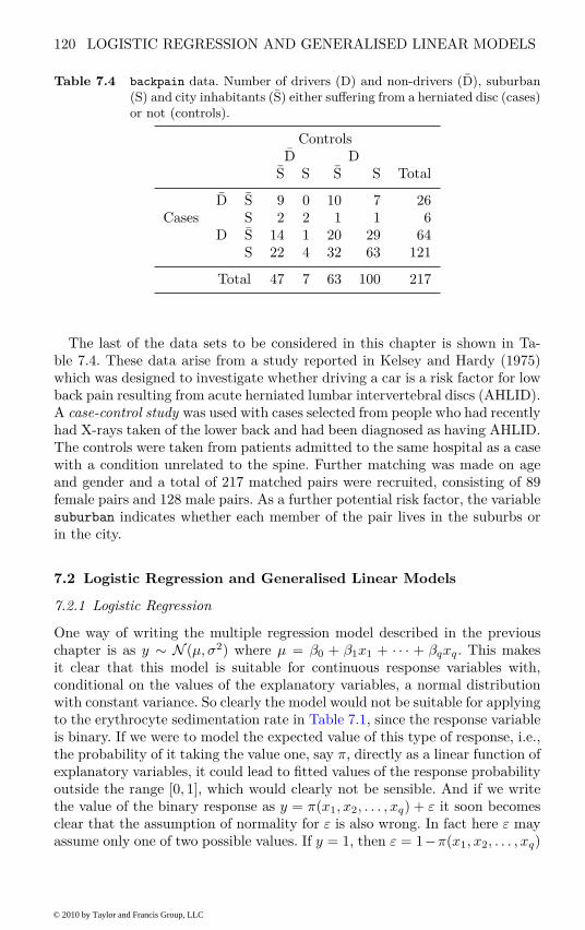
120 LOGISTIC REGRESSION AND GENERALISED LINEAR MODELS
Table 7.4 backpain data. Number of drivers (D) and non-drivers (D), suburban
(S) and city inhabitants (S) either suffering from a herniated disc (cases)
or not (controls).
ControlsD D
S S S S Total
D S 9 0 10 7 26Cases S 2 2 1 1 6
D S 14 1 20 29 64S 22 4 32 63 121
Total 47 7 63 100 217
The last of the data sets to be considered in this chapter is shown in Ta-ble 7.4. These data arise from a study reported in Kelsey and Hardy (1975)which was designed to investigate whether driving a car is a risk factor for lowback pain resulting from acute herniated lumbar intervertebral discs (AHLID).A case-control study was used with cases selected from people who had recentlyhad X-rays taken of the lower back and had been diagnosed as having AHLID.The controls were taken from patients admitted to the same hospital as a casewith a condition unrelated to the spine. Further matching was made on ageand gender and a total of 217 matched pairs were recruited, consisting of 89female pairs and 128 male pairs. As a further potential risk factor, the variablesuburban indicates whether each member of the pair lives in the suburbs orin the city.
7.2 Logistic Regression and Generalised Linear Models
7.2.1 Logistic Regression
One way of writing the multiple regression model described in the previouschapter is as y ∼ N (µ, σ2) where µ = β0 + β1x1 + · · · + βqxq. This makesit clear that this model is suitable for continuous response variables with,conditional on the values of the explanatory variables, a normal distributionwith constant variance. So clearly the model would not be suitable for applyingto the erythrocyte sedimentation rate in Table 7.1, since the response variableis binary. If we were to model the expected value of this type of response, i.e.,the probability of it taking the value one, say π, directly as a linear function ofexplanatory variables, it could lead to fitted values of the response probabilityoutside the range [0, 1], which would clearly not be sensible. And if we writethe value of the binary response as y = π(x1, x2, . . . , xq) + ε it soon becomesclear that the assumption of normality for ε is also wrong. In fact here ε mayassume only one of two possible values. If y = 1, then ε = 1−π(x1, x2, . . . , xq)
© 2010 by Taylor and Francis Group, LLC
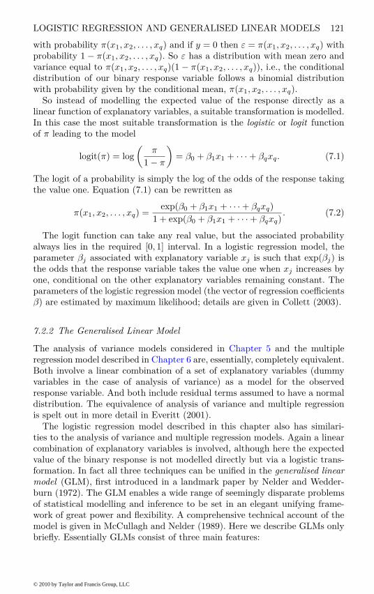
LOGISTIC REGRESSION AND GENERALISED LINEAR MODELS 121
with probability π(x1, x2, . . . , xq) and if y = 0 then ε = π(x1, x2, . . . , xq) withprobability 1 − π(x1, x2, . . . , xq). So ε has a distribution with mean zero andvariance equal to π(x1, x2, . . . , xq)(1 − π(x1, x2, . . . , xq)), i.e., the conditionaldistribution of our binary response variable follows a binomial distributionwith probability given by the conditional mean, π(x1, x2, . . . , xq).
So instead of modelling the expected value of the response directly as alinear function of explanatory variables, a suitable transformation is modelled.In this case the most suitable transformation is the logistic or logit functionof π leading to the model
logit(π) = log
(
π
1 − π
)
= β0 + β1x1 + · · · + βqxq. (7.1)
The logit of a probability is simply the log of the odds of the response takingthe value one. Equation (7.1) can be rewritten as
π(x1, x2, . . . , xq) =exp(β0 + β1x1 + · · · + βqxq)
1 + exp(β0 + β1x1 + · · · + βqxq). (7.2)
The logit function can take any real value, but the associated probabilityalways lies in the required [0, 1] interval. In a logistic regression model, theparameter βj associated with explanatory variable xj is such that exp(βj) isthe odds that the response variable takes the value one when xj increases byone, conditional on the other explanatory variables remaining constant. Theparameters of the logistic regression model (the vector of regression coefficientsβ) are estimated by maximum likelihood; details are given in Collett (2003).
7.2.2 The Generalised Linear Model
The analysis of variance models considered in Chapter 5 and the multipleregression model described in Chapter 6 are, essentially, completely equivalent.Both involve a linear combination of a set of explanatory variables (dummyvariables in the case of analysis of variance) as a model for the observedresponse variable. And both include residual terms assumed to have a normaldistribution. The equivalence of analysis of variance and multiple regressionis spelt out in more detail in Everitt (2001).
The logistic regression model described in this chapter also has similari-ties to the analysis of variance and multiple regression models. Again a linearcombination of explanatory variables is involved, although here the expectedvalue of the binary response is not modelled directly but via a logistic trans-formation. In fact all three techniques can be unified in the generalised linear
model (GLM), first introduced in a landmark paper by Nelder and Wedder-burn (1972). The GLM enables a wide range of seemingly disparate problemsof statistical modelling and inference to be set in an elegant unifying frame-work of great power and flexibility. A comprehensive technical account of themodel is given in McCullagh and Nelder (1989). Here we describe GLMs onlybriefly. Essentially GLMs consist of three main features:
© 2010 by Taylor and Francis Group, LLC

122 LOGISTIC REGRESSION AND GENERALISED LINEAR MODELS
1. An error distribution giving the distribution of the response around itsmean. For analysis of variance and multiple regression this will be the nor-mal; for logistic regression it is the binomial. Each of these (and othersused in other situations to be described later) come from the same, expo-
nential family of probability distributions, and it is this family that is usedin generalised linear modelling (see Everitt and Pickles, 2000).
2. A link function, g, that shows how the linear function of the explanatoryvariables is related to the expected value of the response:
g(µ) = β0 + β1x1 + · · · + βqxq.
For analysis of variance and multiple regression the link function is simplythe identity function; in logistic regression it is the logit function.
3. The variance function that captures how the variance of the response vari-able depends on the mean. We will return to this aspect of GLMs later inthe chapter.
Estimation of the parameters in a GLM is usually achieved through a max-imum likelihood approach – see McCullagh and Nelder (1989) for details.Having estimated a GLM for a data set, the question of the quality of its fitarises. Clearly the investigator needs to be satisfied that the chosen model de-scribes the data adequately, before drawing conclusions about the parameterestimates themselves. In practise, most interest will lie in comparing the fit ofcompeting models, particularly in the context of selecting subsets of explana-tory variables that describe the data in a parsimonious manner. In GLMs ameasure of fit is provided by a quantity known as the deviance which measureshow closely the model-based fitted values of the response approximate the ob-served value. Comparing the deviance values for two models gives a likelihoodratio test of the two models that can be compared by using a statistic having aχ2-distribution with degrees of freedom equal to the difference in the numberof parameters estimated under each model. More details are given in Cook(1998).
7.3 Analysis Using R
7.3.1 ESR and Plasma Proteins
We begin by looking at the ESR data from Table 7.1. As always it is good prac-tise to begin with some simple graphical examination of the data before under-taking any formal modelling. Here we will look at conditional density plots ofthe response variable given the two explanatory variables; such plots describehow the conditional distribution of the categorical variable ESR changes asthe numerical variables fibrinogen and gamma globulin change. The requiredR code to construct these plots is shown with Figure 7.1. It appears that higherlevels of each protein are associated with ESR values above 20 mm/hr.
We can now fit a logistic regression model to the data using the glm func-
© 2010 by Taylor and Francis Group, LLC

ANALYSIS USING R 123
R> data("plasma", package = "HSAUR2")
R> layout(matrix(1:2, ncol = 2))
R> cdplot(ESR ~ fibrinogen, data = plasma)
R> cdplot(ESR ~ globulin, data = plasma)
fibrinogen
ES
R
2.5 3.5 4.5
ES
R <
20
ES
R >
20
0.0
0.2
0.4
0.6
0.8
1.0
globulin
ES
R
30 35 40 45
ES
R <
20
ES
R >
20
0.0
0.2
0.4
0.6
0.8
1.0
Figure 7.1 Conditional density plots of the erythrocyte sedimentation rate (ESR)
given fibrinogen and globulin.
tion. We start with a model that includes only a single explanatory variable,fibrinogen. The code to fit the model is
R> plasma_glm_1 <- glm(ESR ~ fibrinogen, data = plasma,
+ family = binomial())
The formula implicitly defines a parameter for the global mean (the inter-cept term) as discussed in Chapter 5 and Chapter 6. The distribution of theresponse is defined by the family argument, a binomial distribution in ourcase. (The default link function when the binomial family is requested is thelogistic function.)
A description of the fitted model can be obtained from the summary methodapplied to the fitted model. The output is shown in Figure 7.2.
From the results in Figure 7.2 we see that the regression coefficient forfibrinogen is significant at the 5% level. An increase of one unit in this vari-able increases the log-odds in favour of an ESR value greater than 20 by anestimated 1.83 with 95% confidence interval
R> confint(plasma_glm_1, parm = "fibrinogen")
2.5 % 97.5 %
0.3387619 3.9984921
© 2010 by Taylor and Francis Group, LLC
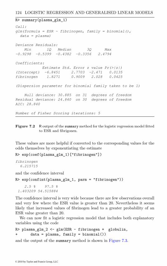
124 LOGISTIC REGRESSION AND GENERALISED LINEAR MODELS
R> summary(plasma_glm_1)
Call:
glm(formula = ESR ~ fibrinogen, family = binomial(),
data = plasma)
Deviance Residuals:
Min 1Q Median 3Q Max
-0.9298 -0.5399 -0.4382 -0.3356 2.4794
Coefficients:
Estimate Std. Error z value Pr(>|z|)
(Intercept) -6.8451 2.7703 -2.471 0.0135
fibrinogen 1.8271 0.9009 2.028 0.0425
(Dispersion parameter for binomial family taken to be 1)
Null deviance: 30.885 on 31 degrees of freedom
Residual deviance: 24.840 on 30 degrees of freedom
AIC: 28.840
Number of Fisher Scoring iterations: 5
Figure 7.2 R output of the summary method for the logistic regression model fitted
to ESR and fibrigonen.
These values are more helpful if converted to the corresponding values for theodds themselves by exponentiating the estimate
R> exp(coef(plasma_glm_1)["fibrinogen"])
fibrinogen
6.215715
and the confidence interval
R> exp(confint(plasma_glm_1, parm = "fibrinogen"))
2.5 % 97.5 %
1.403209 54.515884
The confidence interval is very wide because there are few observations overalland very few where the ESR value is greater than 20. Nevertheless it seemslikely that increased values of fibrinogen lead to a greater probability of anESR value greater than 20.
We can now fit a logistic regression model that includes both explanatoryvariables using the code
R> plasma_glm_2 <- glm(ESR ~ fibrinogen + globulin,
+ data = plasma, family = binomial())
and the output of the summary method is shown in Figure 7.3.
© 2010 by Taylor and Francis Group, LLC
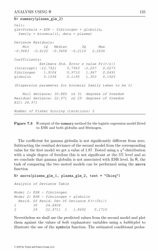
ANALYSIS USING R 125
R> summary(plasma_glm_2)
Call:
glm(formula = ESR ~ fibrinogen + globulin,
family = binomial(), data = plasma)
Deviance Residuals:
Min 1Q Median 3Q Max
-0.9683 -0.6122 -0.3458 -0.2116 2.2636
Coefficients:
Estimate Std. Error z value Pr(>|z|)
(Intercept) -12.7921 5.7963 -2.207 0.0273
fibrinogen 1.9104 0.9710 1.967 0.0491
globulin 0.1558 0.1195 1.303 0.1925
(Dispersion parameter for binomial family taken to be 1)
Null deviance: 30.885 on 31 degrees of freedom
Residual deviance: 22.971 on 29 degrees of freedom
AIC: 28.971
Number of Fisher Scoring iterations: 5
Figure 7.3 R output of the summary method for the logistic regression model fitted
to ESR and both globulin and fibrinogen.
The coefficient for gamma globulin is not significantly different from zero.Subtracting the residual deviance of the second model from the correspondingvalue for the first model we get a value of 1.87. Tested using a χ2-distributionwith a single degree of freedom this is not significant at the 5% level and sowe conclude that gamma globulin is not associated with ESR level. In R, thetask of comparing the two nested models can be performed using the anova
function
R> anova(plasma_glm_1, plasma_glm_2, test = "Chisq")
Analysis of Deviance Table
Model 1: ESR ~ fibrinogen
Model 2: ESR ~ fibrinogen + globulin
Resid. Df Resid. Dev Df Deviance P(>|Chi|)
1 30 24.8404
2 29 22.9711 1 1.8692 0.1716
Nevertheless we shall use the predicted values from the second model and plotthem against the values of both explanatory variables using a bubbleplot toillustrate the use of the symbols function. The estimated conditional proba-
© 2010 by Taylor and Francis Group, LLC

126 LOGISTIC REGRESSION AND GENERALISED LINEAR MODELS
R> plot(globulin ~ fibrinogen, data = plasma, xlim = c(2, 6),
+ ylim = c(25, 55), pch = ".")
R> symbols(plasma$fibrinogen, plasma$globulin, circles = prob,
+ add = TRUE)
2 3 4 5 6
25
30
35
40
45
50
55
fibrinogen
glo
bu
lin
Figure 7.4 Bubbleplot of fitted values for a logistic regression model fitted to the
plasma data.
bility of a ESR value larger 20 for all observations can be computed, followingformula (7.2), by
R> prob <- predict(plasma_glm_2, type = "response")
and now we can assign a larger circle to observations with larger probabilityas shown in Figure 7.4. The plot clearly shows the increasing probability ofan ESR value above 20 (larger circles) as the values of fibrinogen, and to alesser extent, gamma globulin, increase.
© 2010 by Taylor and Francis Group, LLC
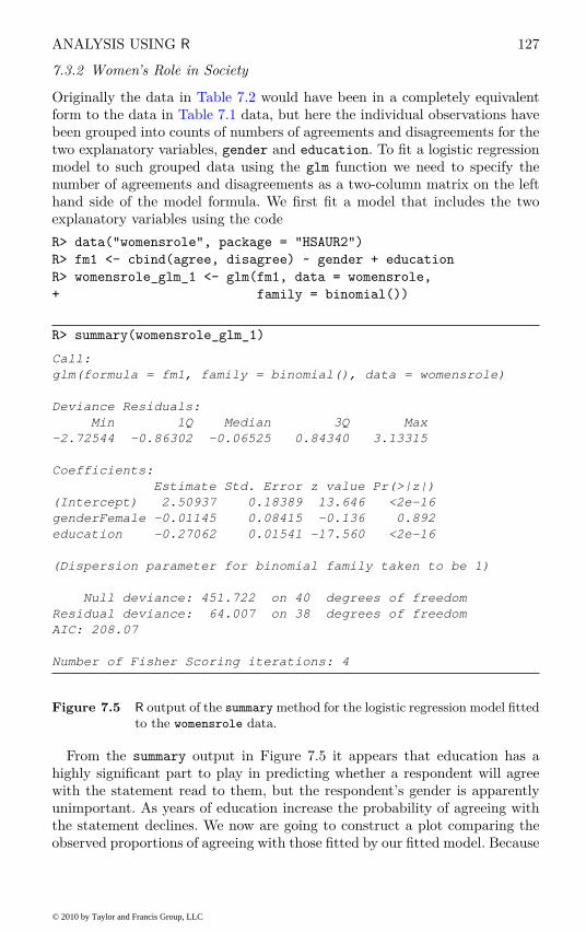
ANALYSIS USING R 127
7.3.2 Women’s Role in Society
Originally the data in Table 7.2 would have been in a completely equivalentform to the data in Table 7.1 data, but here the individual observations havebeen grouped into counts of numbers of agreements and disagreements for thetwo explanatory variables, gender and education. To fit a logistic regressionmodel to such grouped data using the glm function we need to specify thenumber of agreements and disagreements as a two-column matrix on the lefthand side of the model formula. We first fit a model that includes the twoexplanatory variables using the code
R> data("womensrole", package = "HSAUR2")
R> fm1 <- cbind(agree, disagree) ~ gender + education
R> womensrole_glm_1 <- glm(fm1, data = womensrole,
+ family = binomial())
R> summary(womensrole_glm_1)
Call:
glm(formula = fm1, family = binomial(), data = womensrole)
Deviance Residuals:
Min 1Q Median 3Q Max
-2.72544 -0.86302 -0.06525 0.84340 3.13315
Coefficients:
Estimate Std. Error z value Pr(>|z|)
(Intercept) 2.50937 0.18389 13.646 <2e-16
genderFemale -0.01145 0.08415 -0.136 0.892
education -0.27062 0.01541 -17.560 <2e-16
(Dispersion parameter for binomial family taken to be 1)
Null deviance: 451.722 on 40 degrees of freedom
Residual deviance: 64.007 on 38 degrees of freedom
AIC: 208.07
Number of Fisher Scoring iterations: 4
Figure 7.5 R output of the summary method for the logistic regression model fitted
to the womensrole data.
From the summary output in Figure 7.5 it appears that education has ahighly significant part to play in predicting whether a respondent will agreewith the statement read to them, but the respondent’s gender is apparentlyunimportant. As years of education increase the probability of agreeing withthe statement declines. We now are going to construct a plot comparing theobserved proportions of agreeing with those fitted by our fitted model. Because
© 2010 by Taylor and Francis Group, LLC

128 LOGISTIC REGRESSION AND GENERALISED LINEAR MODELS
we will reuse this plot for another fitted object later on, we define a functionwhich plots years of education against some fitted probabilities, e.g.,
R> role.fitted1 <- predict(womensrole_glm_1, type = "response")
and labels each observation with the person’s gender:
1 R> myplot <- function(role.fitted) {
2 + f <- womensrole$gender == "Female"
3 + plot(womensrole$education, role.fitted, type = "n",
4 + ylab = "Probability of agreeing",
5 + xlab = "Education", ylim = c(0,1))
6 + lines(womensrole$education[!f], role.fitted[!f], lty = 1)
7 + lines(womensrole$education[f], role.fitted[f], lty = 2)
8 + lgtxt <- c("Fitted (Males)", "Fitted (Females)")
9 + legend("topright", lgtxt, lty = 1:2, bty = "n")
10 + y <- womensrole$agree / (womensrole$agree +
11 + womensrole$disagree)
12 + text(womensrole$education, y, ifelse(f, "\\VE", "\\MA"),
13 + family = "HersheySerif", cex = 1.25)
14 + }
In lines 3–5 of function myplot, an empty scatterplot of education and fittedprobabilities (type = "n") is set up, basically to set the scene for the followingplotting actions. Then, two lines are drawn (using function lines in lines 6and 7), one for males (with line type 1) and one for females (with line type 2,i.e., a dashed line), where the logical vector f describes both genders. In line9 a legend is added. Finally, in lines 12 and 13 we plot ‘observed’ values, i.e.,the frequencies of agreeing in each of the groups (y as computed in lines 10and 11) and use the Venus and Mars symbols to indicate gender.
The two curves for males and females in Figure 7.6 are almost the samereflecting the non-significant value of the regression coefficient for gender inwomensrole_glm_1. But the observed values plotted on Figure 7.6 suggestthat there might be an interaction of education and gender, a possibility thatcan be investigated by applying a further logistic regression model using
R> fm2 <- cbind(agree,disagree) ~ gender * education
R> womensrole_glm_2 <- glm(fm2, data = womensrole,
+ family = binomial())
The gender and education interaction term is seen to be highly significant,as can be seen from the summary output in Figure 7.7.
Interpreting this interaction effect is made simpler if we again plot fittedand observed values using the same code as previously after getting fittedvalues from womensrole_glm_2. The plot is shown in Figure 7.8. We see thatfor fewer years of education women have a higher probability of agreeing withthe statement than men, but when the years of education exceed about tenthen this situation reverses.
A range of residuals and other diagnostics is available for use in associationwith logistic regression to check whether particular components of the model
© 2010 by Taylor and Francis Group, LLC

ANALYSIS USING R 129
R> myplot(role.fitted1)
0 5 10 15 20
0.0
0.2
0.4
0.6
0.8
1.0
Education
Pro
ba
bili
ty o
f a
gre
ein
g
Fitted (Males)Fitted (Females)
Figure 7.6 Fitted (from womensrole_glm_1) and observed probabilities of agree-
ing for the womensrole data.
are adequate. A comprehensive account of these is given in Collett (2003); herewe shall demonstrate only the use of what is known as the deviance residual.This is the signed square root of the contribution of the ith observation to theoverall deviance. Explicitly it is given by
di = sign(yi − yi)
(
2yi log
(
yi
yi
)
+ 2(ni − yi) log
(
ni − yi
ni − yi
))1/2
(7.3)
where sign is the function that makes di positive when yi ≥ yi and nega-tive else. In (7.3) yi is the observed number of ones for the ith observation(the number of people who agree for each combination of covariates in ourexample), and yi is its fitted value from the model. The residual providesinformation about how well the model fits each particular observation.
© 2010 by Taylor and Francis Group, LLC

130 LOGISTIC REGRESSION AND GENERALISED LINEAR MODELS
R> summary(womensrole_glm_2)
Call:
glm(formula = fm2, family = binomial(), data = womensrole)
Deviance Residuals:
Min 1Q Median 3Q Max
-2.39097 -0.88062 0.01532 0.72783 2.45262
Coefficients:
Estimate Std. Error z value Pr(>|z|)
(Intercept) 2.09820 0.23550 8.910 < 2e-16
genderFemale 0.90474 0.36007 2.513 0.01198
education -0.23403 0.02019 -11.592 < 2e-16
genderFemale:education -0.08138 0.03109 -2.617 0.00886
(Dispersion parameter for binomial family taken to be 1)
Null deviance: 451.722 on 40 degrees of freedom
Residual deviance: 57.103 on 37 degrees of freedom
AIC: 203.16
Number of Fisher Scoring iterations: 4
Figure 7.7 R output of the summary method for the logistic regression model fitted
to the womensrole data.
We can obtain a plot of deviance residuals plotted against fitted values usingthe following code above Figure 7.9. The residuals fall into a horizontal bandbetween −2 and 2. This pattern does not suggest a poor fit for any particularobservation or subset of observations.
7.3.3 Colonic Polyps
The data on colonic polyps in Table 7.3 involves count data. We could try tomodel this using multiple regression but there are two problems. The first isthat a response that is a count can take only positive values, and secondlysuch a variable is unlikely to have a normal distribution. Instead we will applya GLM with a log link function, ensuring that fitted values are positive, anda Poisson error distribution, i.e.,
P(y) =e−λλy
y!.
This type of GLM is often known as Poisson regression. We can apply themodel using
© 2010 by Taylor and Francis Group, LLC

ANALYSIS USING R 131
R> role.fitted2 <- predict(womensrole_glm_2, type = "response")
R> myplot(role.fitted2)
0 5 10 15 20
0.0
0.2
0.4
0.6
0.8
1.0
Education
Pro
ba
bili
ty o
f a
gre
ein
g
Fitted (Males)Fitted (Females)
Figure 7.8 Fitted (from womensrole_glm_2) and observed probabilities of agree-
ing for the womensrole data.
R> data("polyps", package = "HSAUR2")
R> polyps_glm_1 <- glm(number ~ treat + age, data = polyps,
+ family = poisson())
(The default link function when the Poisson family is requested is the logfunction.)
From Figure 7.10 we see that the regression coefficients for both age andtreatment are highly significant. But there is a problem with the model, butbefore we can deal with it we need a short digression to describe in more detailthe third component of GLMs mentioned in the previous section, namely theirvariance functions, V (µ).
© 2010 by Taylor and Francis Group, LLC

132 LOGISTIC REGRESSION AND GENERALISED LINEAR MODELS
R> res <- residuals(womensrole_glm_2, type = "deviance")
R> plot(predict(womensrole_glm_2), res,
+ xlab="Fitted values", ylab = "Residuals",
+ ylim = max(abs(res)) * c(-1,1))
R> abline(h = 0, lty = 2)
−3 −2 −1 0 1 2 3
−2
−1
01
2
Fitted values
Re
sid
ua
ls
Figure 7.9 Plot of deviance residuals from logistic regression model fitted to the
womensrole data.
The variance function of a GLM captures how the variance of a responsevariable depends upon its mean. The general form of the relationship is
Var(response) = φV (µ)
where φ is constant and V (µ) specifies how the variance depends on the mean.For the error distributions considered previously this general form becomes:
Normal: V (µ) = 1, φ = σ2; here the variance does not depend on the mean.
Binomial: V (µ) = µ(1 − µ), φ = 1.
© 2010 by Taylor and Francis Group, LLC

ANALYSIS USING R 133
R> summary(polyps_glm_1)
Call:
glm(formula = number ~ treat + age, family = poisson(),
data = polyps)
Deviance Residuals:
Min 1Q Median 3Q Max
-4.2212 -3.0536 -0.1802 1.4459 5.8301
Coefficients:
Estimate Std. Error z value Pr(>|z|)
(Intercept) 4.529024 0.146872 30.84 < 2e-16
treatdrug -1.359083 0.117643 -11.55 < 2e-16
age -0.038830 0.005955 -6.52 7.02e-11
(Dispersion parameter for poisson family taken to be 1)
Null deviance: 378.66 on 19 degrees of freedom
Residual deviance: 179.54 on 17 degrees of freedom
AIC: 273.88
Number of Fisher Scoring iterations: 5
Figure 7.10 R output of the summary method for the Poisson regression model
fitted to the polyps data.
Poisson: V (µ) = µ, φ = 1.
In the case of a Poisson variable we see that the mean and variance are equal,and in the case of a binomial variable where the mean is the probability ofthe variable taking the value one, π, the variance is π(1 − π).
Both the Poisson and binomial distributions have variance functions thatare completely determined by the mean. There is no free parameter for thevariance since, in applications of the generalised linear model with binomialor Poisson error distributions the dispersion parameter, φ, is defined to be one(see previous results for logistic and Poisson regression). But in some applica-tions this becomes too restrictive to fully account for the empirical variance inthe data; in such cases it is common to describe the phenomenon as overdisper-
sion. For example, if the response variable is the proportion of family memberswho have been ill in the past year, observed in a large number of families, thenthe individual binary observations that make up the observed proportions arelikely to be correlated rather than independent. The non-independence canlead to a variance that is greater (less) than on the assumption of binomialvariability. And observed counts often exhibit larger variance than would beexpected from the Poisson assumption, a fact noted over 80 years ago byGreenwood and Yule (1920).
© 2010 by Taylor and Francis Group, LLC

134 LOGISTIC REGRESSION AND GENERALISED LINEAR MODELS
When fitting generalised models with binomial or Poisson error distribu-tions, overdispersion can often be spotted by comparing the residual deviancewith its degrees of freedom. For a well-fitting model the two quantities shouldbe approximately equal. If the deviance is far greater than the degrees offreedom overdispersion may be indicated. This is the case for the results inFigure 7.10. So what can we do?
We can deal with overdispersion by using a procedure known as quasi-
likelihood, which allows the estimation of model parameters without fullyknowing the error distribution of the response variable. McCullagh and Nelder(1989) give full details of the quasi-likelihood approach. In many respects itsimply allows for the estimation of φ from the data rather than defining itto be unity for the binomial and Poisson distributions. We can apply quasi-likelihood estimation to the colonic polyps data using the following R code
R> polyps_glm_2 <- glm(number ~ treat + age, data = polyps,
+ family = quasipoisson())
R> summary(polyps_glm_2)
Call:
glm(formula = number ~ treat + age,
family = quasipoisson(), data = polyps)
Deviance Residuals:
Min 1Q Median 3Q Max
-4.2212 -3.0536 -0.1802 1.4459 5.8301
Coefficients:
Estimate Std. Error t value Pr(>|t|)
(Intercept) 4.52902 0.48106 9.415 3.72e-08
treatdrug -1.35908 0.38533 -3.527 0.00259
age -0.03883 0.01951 -1.991 0.06284
(Dispersion parameter for quasipoisson family taken to be 10.73)
Null deviance: 378.66 on 19 degrees of freedom
Residual deviance: 179.54 on 17 degrees of freedom
AIC: NA
Number of Fisher Scoring iterations: 5
The regression coefficients for both explanatory variables remain significantbut their estimated standard errors are now much greater than the valuesgiven in Figure 7.10. A possible reason for overdispersion in these data is thatpolyps do not occur independently of one another, but instead may ‘cluster’together.
© 2010 by Taylor and Francis Group, LLC

ANALYSIS USING R 135
7.3.4 Driving and Back Pain
A frequently used design in medicine is the matched case-control study inwhich each patient suffering from a particular condition of interest includedin the study is matched to one or more people without the condition. The mostcommonly used matching variables are age, ethnic group, mental status etc. Adesign with m controls per case is known as a 1 : m matched study. In manycases m will be one, and it is the 1 : 1 matched study that we shall concentrateon here where we analyse the data on low back pain given in Table 7.4. Tobegin we shall describe the form of the logistic model appropriate for case-control studies in the simplest case where there is only one binary explanatoryvariable.
With matched pairs data the form of the logistic model involves the proba-bility, ϕ, that in matched pair number i, for a given value of the explanatoryvariable the member of the pair is a case. Specifically the model is
logit(ϕi) = αi + βx.
The odds that a subject with x = 1 is a case equals exp(β) times the oddsthat a subject with x = 0 is a case.
The model generalises to the situation where there are q explanatory vari-ables as
logit(ϕi) = αi + β1x1 + β2x2 + . . . βqxq.
Typically one x is an explanatory variable of real interest, such as pastexposure to a risk factor, with the others being used as a form of statisticalcontrol in addition to the variables already controlled by virtue of using themto form matched pairs. This is the case in our back pain example where it isthe effect of car driving on lower back pain that is of most interest.
The problem with the model above is that the number of parameters in-creases at the same rate as the sample size with the consequence that maxi-mum likelihood estimation is no longer viable. We can overcome this problemif we regard the parameters αi as of little interest and so are willing to forgotheir estimation. If we do, we can then create a conditional likelihood function
that will yield maximum likelihood estimators of the coefficients, β1, . . . , βq,that are consistent and asymptotically normally distributed. The mathematicsbehind this are described in Collett (2003).
The model can be fitted using the clogit function from package survival;the results are shown in Figure 7.11.
R> library("survival")
R> backpain_glm <- clogit(I(status == "case") ~
+ driver + suburban + strata(ID), data = backpain)
The response has to be a logical (TRUE for cases) and the strata commandspecifies the matched pairs.
The estimate of the odds ratio of a herniated disc occurring in a driverrelative to a nondriver is 1.93 with a 95% confidence interval of (1.09, 3.44).
© 2010 by Taylor and Francis Group, LLC
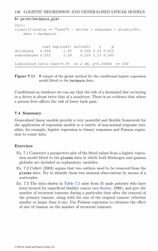
136 LOGISTIC REGRESSION AND GENERALISED LINEAR MODELS
R> print(backpain_glm)
Call:
clogit(I(status == "case") ~ driver + suburban + strata(ID),
data = backpain)
coef exp(coef) se(coef) z p
driveryes 0.658 1.93 0.294 2.24 0.025
suburbanyes 0.255 1.29 0.226 1.13 0.260
Likelihood ratio test=9.55 on 2 df, p=0.00846 n= 434
Figure 7.11 R output of the print method for the conditional logistic regression
model fitted to the backpain data.
Conditional on residence we can say that the risk of a herniated disc occurringin a driver is about twice that of a nondriver. There is no evidence that wherea person lives affects the risk of lower back pain.
7.4 Summary
Generalised linear models provide a very powerful and flexible framework forthe application of regression models to a variety of non-normal response vari-ables, for example, logistic regression to binary responses and Poisson regres-sion to count data.
Exercises
Ex. 7.1 Construct a perspective plot of the fitted values from a logistic regres-sion model fitted to the plasma data in which both fibrinogen and gammaglobulin are included as explanatory variables.
Ex. 7.2 Collett (2003) argues that two outliers need to be removed from theplasma data. Try to identify those two unusual observations by means of ascatterplot.
Ex. 7.3 The data shown in Table 7.5 arise from 31 male patients who havebeen treated for superficial bladder cancer (see Seeber, 1998), and give thenumber of recurrent tumours during a particular time after the removal ofthe primary tumour, along with the size of the original tumour (whethersmaller or larger than 3 cm). Use Poisson regression to estimate the effectof size of tumour on the number of recurrent tumours.
© 2010 by Taylor and Francis Group, LLC

SUMMARY 137
Table 7.5: bladdercancer data. Number of recurrent tumoursfor bladder cancer patients.
time tumorsize number time tumorsize number
2 <=3cm 1 13 <=3cm 23 <=3cm 1 15 <=3cm 26 <=3cm 1 18 <=3cm 28 <=3cm 1 23 <=3cm 29 <=3cm 1 20 <=3cm 3
10 <=3cm 1 24 <=3cm 411 <=3cm 1 1 >3cm 113 <=3cm 1 5 >3cm 114 <=3cm 1 17 >3cm 116 <=3cm 1 18 >3cm 121 <=3cm 1 25 >3cm 122 <=3cm 1 18 >3cm 224 <=3cm 1 25 >3cm 226 <=3cm 1 4 >3cm 327 <=3cm 1 19 >3cm 47 <=3cm 2
Source: From Seeber, G. U. H., in Encyclopedia of Biostatistics, John Wiley& Sons, Chichester, UK, 1998. With permission.
Ex. 7.4 The data in Table 7.6 show the survival times from diagnosis of pa-tients suffering from leukemia and the values of two explanatory variables,the white blood cell count (wbc) and the presence or absence of a morpho-logical characteristic of the white blood cells (ag) (the data are availablein package MASS, Venables and Ripley, 2002). Define a binary outcomevariable according to whether or not patients lived for at least 24 weeks af-ter diagnosis and then fit a logistic regression model to the data. It may beadvisable to transform the very large white blood counts to avoid regressioncoefficients very close to 0 (and odds ratios very close to 1). And a modelthat contains only the two explanatory variables may not be adequate forthese data. Construct some graphics useful in the interpretation of the finalmodel you fit.
© 2010 by Taylor and Francis Group, LLC
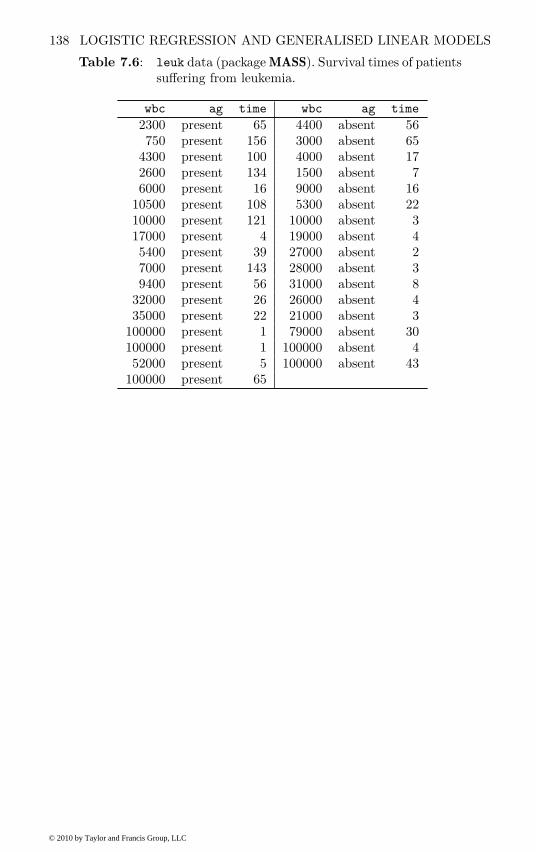
138 LOGISTIC REGRESSION AND GENERALISED LINEAR MODELS
Table 7.6: leuk data (package MASS). Survival times of patientssuffering from leukemia.
wbc ag time wbc ag time
2300 present 65 4400 absent 56750 present 156 3000 absent 65
4300 present 100 4000 absent 172600 present 134 1500 absent 76000 present 16 9000 absent 16
10500 present 108 5300 absent 2210000 present 121 10000 absent 317000 present 4 19000 absent 45400 present 39 27000 absent 27000 present 143 28000 absent 39400 present 56 31000 absent 8
32000 present 26 26000 absent 435000 present 22 21000 absent 3
100000 present 1 79000 absent 30100000 present 1 100000 absent 452000 present 5 100000 absent 43
100000 present 65
© 2010 by Taylor and Francis Group, LLC
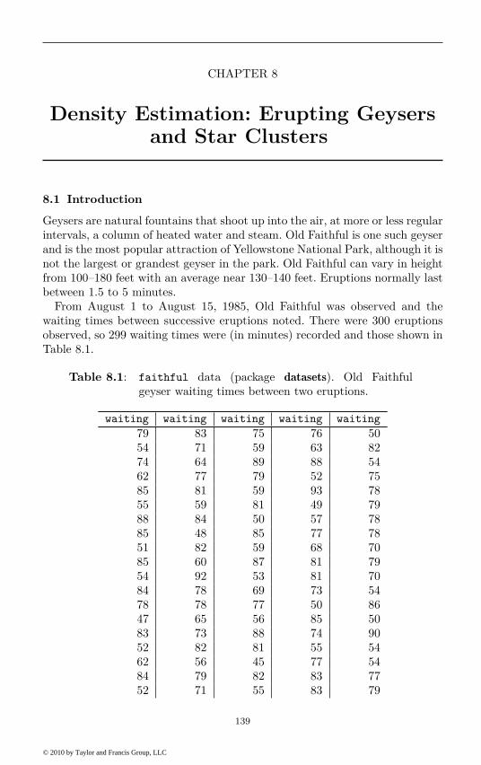
CHAPTER 8
Density Estimation: Erupting Geysersand Star Clusters
8.1 Introduction
Geysers are natural fountains that shoot up into the air, at more or less regularintervals, a column of heated water and steam. Old Faithful is one such geyserand is the most popular attraction of Yellowstone National Park, although it isnot the largest or grandest geyser in the park. Old Faithful can vary in heightfrom 100–180 feet with an average near 130–140 feet. Eruptions normally lastbetween 1.5 to 5 minutes.
From August 1 to August 15, 1985, Old Faithful was observed and thewaiting times between successive eruptions noted. There were 300 eruptionsobserved, so 299 waiting times were (in minutes) recorded and those shown inTable 8.1.
Table 8.1: faithful data (package datasets). Old Faithfulgeyser waiting times between two eruptions.
waiting waiting waiting waiting waiting
79 83 75 76 5054 71 59 63 8274 64 89 88 5462 77 79 52 7585 81 59 93 7855 59 81 49 7988 84 50 57 7885 48 85 77 7851 82 59 68 7085 60 87 81 7954 92 53 81 7084 78 69 73 5478 78 77 50 8647 65 56 85 5083 73 88 74 9052 82 81 55 5462 56 45 77 5484 79 82 83 7752 71 55 83 79
139
© 2010 by Taylor and Francis Group, LLC

140 DENSITY ESTIMATION
Table 8.1: faithful data (continued).
waiting waiting waiting waiting waiting
79 62 90 51 6451 76 45 78 7547 60 83 84 4778 78 56 46 8669 76 89 83 6374 83 46 55 8583 75 82 81 8255 82 51 57 5776 70 86 76 8278 65 53 84 6779 73 79 77 7473 88 81 81 5477 76 60 87 8366 80 82 77 7380 48 77 51 7374 86 76 78 8852 60 59 60 8048 90 80 82 7180 50 49 91 8359 78 96 53 5690 63 53 78 7980 72 77 46 7858 84 77 77 8484 75 65 84 5858 51 81 49 8373 82 71 83 4383 62 70 71 6064 88 81 80 7553 49 93 49 8182 83 53 75 4659 81 89 64 9075 47 45 76 4690 84 86 53 7454 52 58 9480 86 78 5554 81 66 76
© 2010 by Taylor and Francis Group, LLC

DENSITY ESTIMATION 141
The Hertzsprung-Russell (H-R) diagram forms the basis of the theory ofstellar evolution. The diagram is essentially a plot of the energy output ofstars plotted against their surface temperature. Data from the H-R diagramof Star Cluster CYG OB1, calibrated according to Vanisma and De Greve(1972) are shown in Table 8.2 (from Hand et al., 1994).
Table 8.2: CYGOB1 data. Energy output and surface temperatureof Star Cluster CYG OB1.
logst logli logst logli logst logli
4.37 5.23 4.23 3.94 4.45 5.224.56 5.74 4.42 4.18 3.49 6.294.26 4.93 4.23 4.18 4.23 4.344.56 5.74 3.49 5.89 4.62 5.624.30 5.19 4.29 4.38 4.53 5.104.46 5.46 4.29 4.22 4.45 5.223.84 4.65 4.42 4.42 4.53 5.184.57 5.27 4.49 4.85 4.43 5.574.26 5.57 4.38 5.02 4.38 4.624.37 5.12 4.42 4.66 4.45 5.063.49 5.73 4.29 4.66 4.50 5.344.43 5.45 4.38 4.90 4.45 5.344.48 5.42 4.22 4.39 4.55 5.544.01 4.05 3.48 6.05 4.45 4.984.29 4.26 4.38 4.42 4.42 4.504.42 4.58 4.56 5.10
8.2 Density Estimation
The goal of density estimation is to approximate the probability density func-tion of a random variable (univariate or multivariate) given a sample of ob-servations of the variable. Univariate histograms are a simple example of adensity estimate; they are often used for two purposes, counting and display-ing the distribution of a variable, but according to Wilkinson (1992), they areeffective for neither. For bivariate data, two-dimensional histograms can beconstructed, but for small and moderate sized data sets that is not of any realuse for estimating the bivariate density function, simply because most of the‘boxes’ in the histogram will contain too few observations, or if the number ofboxes is reduced the resulting histogram will be too coarse a representationof the density function.
The density estimates provided by one- and two-dimensional histograms canbe improved on in a number of ways. If, of course, we are willing to assume aparticular form for the variable’s distribution, for example, Gaussian, density
© 2010 by Taylor and Francis Group, LLC

142 DENSITY ESTIMATION
estimation would be reduced to estimating the parameters of the assumeddistribution. More commonly, however, we wish to allow the data to speak forthemselves and so one of a variety of non-parametric estimation proceduresthat are now available might be used. Density estimation is covered in detailin several books, including Silverman (1986), Scott (1992), Wand and Jones(1995) and Simonoff (1996). One of the most popular classes of proceduresis the kernel density estimators, which we now briefly describe for univariateand bivariate data.
8.2.1 Kernel Density Estimators
From the definition of a probability density, if the random X has a density f ,
f(x) = limh→0
1
2hP(x − h < X < x + h). (8.1)
For any given h a naıve estimator of P(x − h < X < x + h) is the proportionof the observations x1, x2, . . . , xn falling in the interval (x − h, x + h), that is
f(x) =1
2hn
n∑
i=1
I(xi ∈ (x − h, x + h)), (8.2)
i.e., the number of x1, . . . , xn falling in the interval (x − h, x + h) divided by2hn. If we introduce a weight function W given by
W (x) =
1
2|x| < 1
0 else
then the naıve estimator can be rewritten as
f(x) =1
n
n∑
i=1
1
hW
(
x − xi
h
)
. (8.3)
Unfortunately this estimator is not a continuous function and is not par-ticularly satisfactory for practical density estimation. It does however leadnaturally to the kernel estimator defined by
f(x) =1
hn
n∑
i=1
K
(
x − xi
h
)
(8.4)
where K is known as the kernel function and h as the bandwidth or smoothing
parameter. The kernel function must satisfy the condition∫
∞
−∞
K(x)dx = 1.
Usually, but not always, the kernel function will be a symmetric density func-tion, for example, the normal. Three commonly used kernel functions are
© 2010 by Taylor and Francis Group, LLC
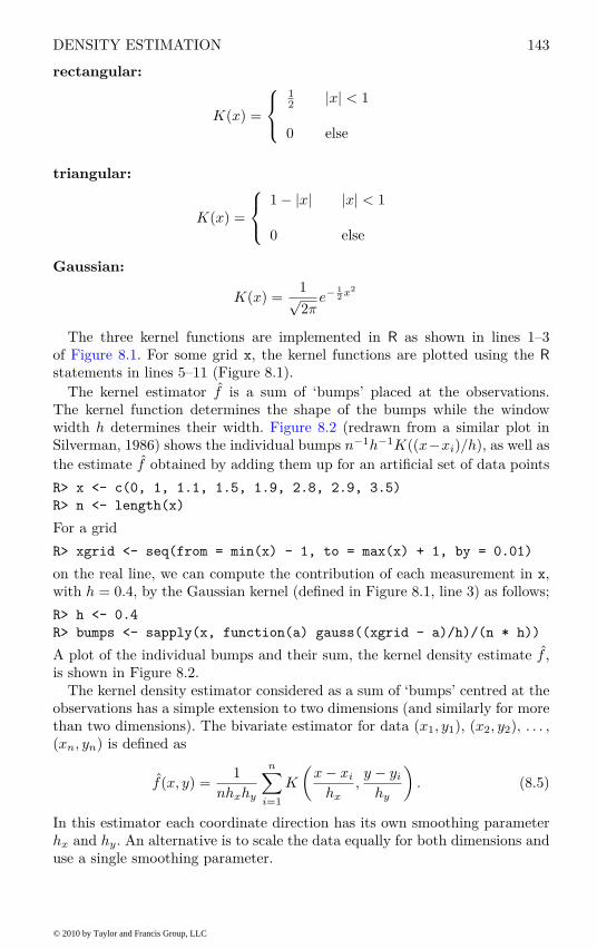
DENSITY ESTIMATION 143
rectangular:
K(x) =
1
2|x| < 1
0 else
triangular:
K(x) =
1 − |x| |x| < 1
0 else
Gaussian:
K(x) =1
√
2πe−
1
2x2
The three kernel functions are implemented in R as shown in lines 1–3of Figure 8.1. For some grid x, the kernel functions are plotted using the R
statements in lines 5–11 (Figure 8.1).
The kernel estimator f is a sum of ‘bumps’ placed at the observations.The kernel function determines the shape of the bumps while the windowwidth h determines their width. Figure 8.2 (redrawn from a similar plot inSilverman, 1986) shows the individual bumps n−1h−1K((x−xi)/h), as well as
the estimate f obtained by adding them up for an artificial set of data points
R> x <- c(0, 1, 1.1, 1.5, 1.9, 2.8, 2.9, 3.5)
R> n <- length(x)
For a grid
R> xgrid <- seq(from = min(x) - 1, to = max(x) + 1, by = 0.01)
on the real line, we can compute the contribution of each measurement in x,with h = 0.4, by the Gaussian kernel (defined in Figure 8.1, line 3) as follows;
R> h <- 0.4
R> bumps <- sapply(x, function(a) gauss((xgrid - a)/h)/(n * h))
A plot of the individual bumps and their sum, the kernel density estimate f ,is shown in Figure 8.2.
The kernel density estimator considered as a sum of ‘bumps’ centred at theobservations has a simple extension to two dimensions (and similarly for morethan two dimensions). The bivariate estimator for data (x1, y1), (x2, y2), . . . ,(xn, yn) is defined as
f(x, y) =1
nhxhy
n∑
i=1
K
(
x − xi
hx
,y − yi
hy
)
. (8.5)
In this estimator each coordinate direction has its own smoothing parameterhx and hy. An alternative is to scale the data equally for both dimensions anduse a single smoothing parameter.
© 2010 by Taylor and Francis Group, LLC
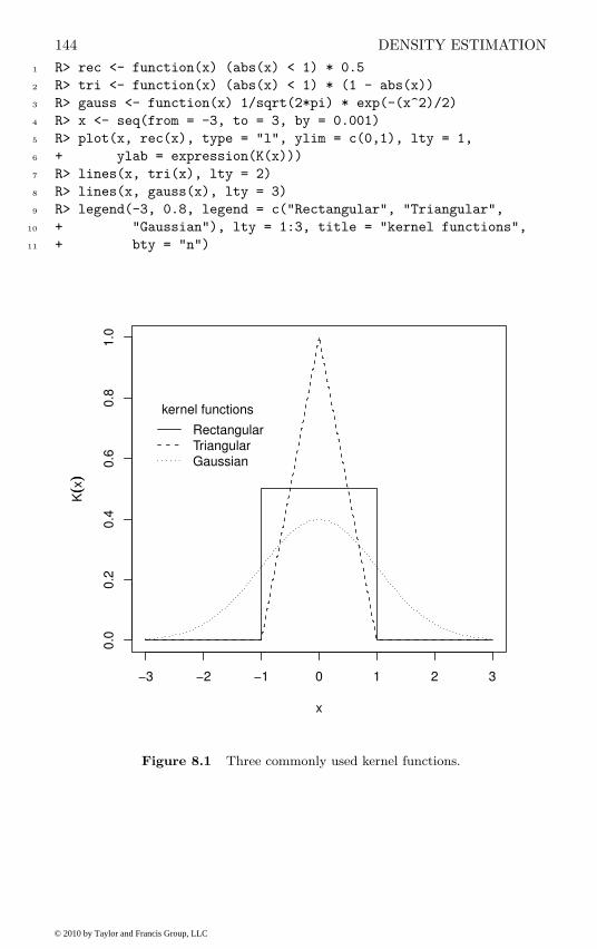
144 DENSITY ESTIMATION
1 R> rec <- function(x) (abs(x) < 1) * 0.5
2 R> tri <- function(x) (abs(x) < 1) * (1 - abs(x))
3 R> gauss <- function(x) 1/sqrt(2*pi) * exp(-(x^2)/2)
4 R> x <- seq(from = -3, to = 3, by = 0.001)
5 R> plot(x, rec(x), type = "l", ylim = c(0,1), lty = 1,
6 + ylab = expression(K(x)))
7 R> lines(x, tri(x), lty = 2)
8 R> lines(x, gauss(x), lty = 3)
9 R> legend(-3, 0.8, legend = c("Rectangular", "Triangular",
10 + "Gaussian"), lty = 1:3, title = "kernel functions",
11 + bty = "n")
−3 −2 −1 0 1 2 3
0.0
0.2
0.4
0.6
0.8
1.0
x
K((x
))
kernel functions
RectangularTriangularGaussian
Figure 8.1 Three commonly used kernel functions.
© 2010 by Taylor and Francis Group, LLC

DENSITY ESTIMATION 145
1 R> plot(xgrid, rowSums(bumps), ylab = expression(hat(f)(x)),
2 + type = "l", xlab = "x", lwd = 2)
3 R> rug(x, lwd = 2)
4 R> out <- apply(bumps, 2, function(b) lines(xgrid, b))
−1 0 1 2 3 4
0.0
00
.05
0.1
00
.15
0.2
00
.25
0.3
00
.35
x
f^ ((x))
Figure 8.2 Kernel estimate showing the contributions of Gaussian kernels evalu-
ated for the individual observations with bandwidth h = 0.4.
For bivariate density estimation a commonly used kernel function is thestandard bivariate normal density
K(x, y) =1
2πe−
1
2(x2
+y2).
Another possibility is the bivariate Epanechnikov kernel given by
K(x, y) =
2
π(1 − x2
− y2) x2 + y2 < 1
0 else
© 2010 by Taylor and Francis Group, LLC

146 DENSITY ESTIMATION
R> epa <- function(x, y)
+ ((x^2 + y^2) < 1) * 2/pi * (1 - x^2 - y^2)
R> x <- seq(from = -1.1, to = 1.1, by = 0.05)
R> epavals <- sapply(x, function(a) epa(a, x))
R> persp(x = x, y = x, z = epavals, xlab = "x", ylab = "y",
+ zlab = expression(K(x, y)), theta = -35, axes = TRUE,
+ box = TRUE)
x
y
K(x
, y)
Figure 8.3 Epanechnikov kernel for a grid between (−1.1,−1.1) and (1.1, 1.1).
which is implemented and depicted in Figure 8.3, here by using the persp
function for plotting in three dimensions.
According to Venables and Ripley (2002) the bandwidth should be chosento be proportional to n−1/5; unfortunately the constant of proportionalitydepends on the unknown density. The tricky problem of bandwidth estimationis considered in detail in Silverman (1986).
© 2010 by Taylor and Francis Group, LLC
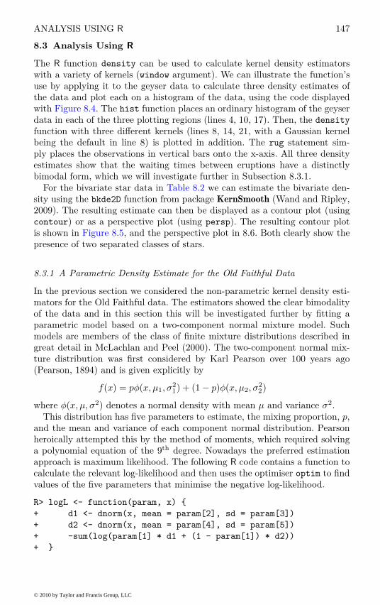
ANALYSIS USING R 147
8.3 Analysis Using R
The R function density can be used to calculate kernel density estimatorswith a variety of kernels (window argument). We can illustrate the function’suse by applying it to the geyser data to calculate three density estimates ofthe data and plot each on a histogram of the data, using the code displayedwith Figure 8.4. The hist function places an ordinary histogram of the geyserdata in each of the three plotting regions (lines 4, 10, 17). Then, the density
function with three different kernels (lines 8, 14, 21, with a Gaussian kernelbeing the default in line 8) is plotted in addition. The rug statement sim-ply places the observations in vertical bars onto the x-axis. All three densityestimates show that the waiting times between eruptions have a distinctlybimodal form, which we will investigate further in Subsection 8.3.1.
For the bivariate star data in Table 8.2 we can estimate the bivariate den-sity using the bkde2D function from package KernSmooth (Wand and Ripley,2009). The resulting estimate can then be displayed as a contour plot (usingcontour) or as a perspective plot (using persp). The resulting contour plotis shown in Figure 8.5, and the perspective plot in 8.6. Both clearly show thepresence of two separated classes of stars.
8.3.1 A Parametric Density Estimate for the Old Faithful Data
In the previous section we considered the non-parametric kernel density esti-mators for the Old Faithful data. The estimators showed the clear bimodalityof the data and in this section this will be investigated further by fitting aparametric model based on a two-component normal mixture model. Suchmodels are members of the class of finite mixture distributions described ingreat detail in McLachlan and Peel (2000). The two-component normal mix-ture distribution was first considered by Karl Pearson over 100 years ago(Pearson, 1894) and is given explicitly by
f(x) = pφ(x, µ1, σ2
1) + (1 − p)φ(x, µ2, σ
2
2)
where φ(x, µ, σ2) denotes a normal density with mean µ and variance σ2.This distribution has five parameters to estimate, the mixing proportion, p,
and the mean and variance of each component normal distribution. Pearsonheroically attempted this by the method of moments, which required solvinga polynomial equation of the 9th degree. Nowadays the preferred estimationapproach is maximum likelihood. The following R code contains a function tocalculate the relevant log-likelihood and then uses the optimiser optim to findvalues of the five parameters that minimise the negative log-likelihood.
R> logL <- function(param, x) {
+ d1 <- dnorm(x, mean = param[2], sd = param[3])
+ d2 <- dnorm(x, mean = param[4], sd = param[5])
+ -sum(log(param[1] * d1 + (1 - param[1]) * d2))
+ }
© 2010 by Taylor and Francis Group, LLC

148 DENSITY ESTIMATION
1 R> data("faithful", package = "datasets")
2 R> x <- faithful$waiting
3 R> layout(matrix(1:3, ncol = 3))
4 R> hist(x, xlab = "Waiting times (in min.)", ylab = "Frequency",
5 + probability = TRUE, main = "Gaussian kernel",
6 + border = "gray")
7 R> lines(density(x, width = 12), lwd = 2)
8 R> rug(x)
9 R> hist(x, xlab = "Waiting times (in min.)", ylab = "Frequency",
10 + probability = TRUE, main = "Rectangular kernel",
11 + border = "gray")
12 R> lines(density(x, width = 12, window = "rectangular"), lwd = 2)
13 R> rug(x)
14 R> hist(x, xlab = "Waiting times (in min.)", ylab = "Frequency",
15 + probability = TRUE, main = "Triangular kernel",
16 + border = "gray")
17 R> lines(density(x, width = 12, window = "triangular"), lwd = 2)
18 R> rug(x)
Gaussian kernel
Waiting times (in min.)
Fre
quency
40 60 80 100
0.0
00.0
10.0
20.0
30.0
4
Rectangular kernel
Waiting times (in min.)
Fre
quency
40 60 80 100
0.0
00.0
10.0
20.0
30.0
4
Triangular kernel
Waiting times (in min.)
Fre
quency
40 60 80 100
0.0
00.0
10.0
20.0
30.0
4
Figure 8.4 Density estimates of the geyser eruption data imposed on a histogram
of the data.
© 2010 by Taylor and Francis Group, LLC
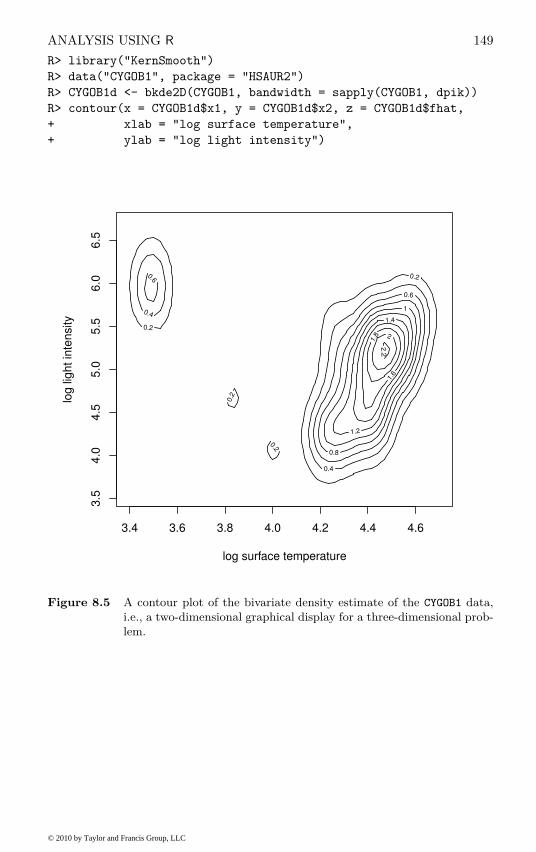
ANALYSIS USING R 149
R> library("KernSmooth")
R> data("CYGOB1", package = "HSAUR2")
R> CYGOB1d <- bkde2D(CYGOB1, bandwidth = sapply(CYGOB1, dpik))
R> contour(x = CYGOB1d$x1, y = CYGOB1d$x2, z = CYGOB1d$fhat,
+ xlab = "log surface temperature",
+ ylab = "log light intensity")
log surface temperature
log
lig
ht
inte
nsity
0.2
0.2
0.2
0.2
0.4
0.4
0.6
0.6
0.8
1
1.2
1.4
1.6
1.8
2
2.2
3.4 3.6 3.8 4.0 4.2 4.4 4.6
3.5
4.0
4.5
5.0
5.5
6.0
6.5
Figure 8.5 A contour plot of the bivariate density estimate of the CYGOB1 data,
i.e., a two-dimensional graphical display for a three-dimensional prob-
lem.
© 2010 by Taylor and Francis Group, LLC
150 DENSITY ESTIMATION
R> persp(x = CYGOB1d$x1, y = CYGOB1d$x2, z = CYGOB1d$fhat,
+ xlab = "log surface temperature",
+ ylab = "log light intensity",
+ zlab = "estimated density",
+ theta = -35, axes = TRUE, box = TRUE)
log surface te
mperature
log light intensity
estim
ate
d d
ensity
Figure 8.6 The bivariate density estimate of the CYGOB1 data, here shown in a
three-dimensional fashion using the persp function.
R> startparam <- c(p = 0.5, mu1 = 50, sd1 = 3, mu2 = 80, sd2 = 3)
R> opp <- optim(startparam, logL, x = faithful$waiting,
+ method = "L-BFGS-B",
+ lower = c(0.01, rep(1, 4)),
+ upper = c(0.99, rep(200, 4)))
R> opp
$par
p mu1 sd1 mu2 sd2
© 2010 by Taylor and Francis Group, LLC

ANALYSIS USING R 151
0.360891 54.612125 5.872379 80.093414 5.867288
$value
[1] 1034.002
$counts
function gradient
55 55
$convergence
[1] 0
Of course, optimising the appropriate likelihood ‘by hand’ is not very con-venient. In fact, (at least) two packages offer high-level functionality for esti-mating mixture models. The first one is package mclust (Fraley et al., 2009)implementing the methodology described in Fraley and Raftery (2002). Here,a Bayesian information criterion (BIC) is applied to choose the form of themixture model:
R> library("mclust")
R> mc <- Mclust(faithful$waiting)
R> mc
best model: equal variance with 2 components
and the estimated means are
R> mc$parameters$mean
1 2
54.61911 80.09384
with estimated standard deviation (found to be equal within both groups)
R> sqrt(mc$parameters$variance$sigmasq)
[1] 5.86848
The proportion is p = 0.36. The second package is called flexmix whose func-tionality is described by Leisch (2004). A mixture of two normals can be fittedusing
R> library("flexmix")
R> fl <- flexmix(waiting ~ 1, data = faithful, k = 2)
with p = 0.36 and estimated parameters
R> parameters(fl, component = 1)
Comp.1
coef.(Intercept) 54.628701
sigma 5.895234
R> parameters(fl, component = 2)
Comp.2
coef.(Intercept) 80.098582
sigma 5.871749
© 2010 by Taylor and Francis Group, LLC

152 DENSITY ESTIMATION
R> opar <- as.list(opp$par)
R> rx <- seq(from = 40, to = 110, by = 0.1)
R> d1 <- dnorm(rx, mean = opar$mu1, sd = opar$sd1)
R> d2 <- dnorm(rx, mean = opar$mu2, sd = opar$sd2)
R> f <- opar$p * d1 + (1 - opar$p) * d2
R> hist(x, probability = TRUE, xlab = "Waiting times (in min.)",
+ border = "gray", xlim = range(rx), ylim = c(0, 0.06),
+ main = "")
R> lines(rx, f, lwd = 2)
R> lines(rx, dnorm(rx, mean = mean(x), sd = sd(x)), lty = 2,
+ lwd = 2)
R> legend(50, 0.06, lty = 1:2, bty = "n",
+ legend = c("Fitted two-component mixture density",
+ "Fitted single normal density"))
Waiting times (in min.)
De
nsity
40 50 60 70 80 90 100 110
0.0
00
.01
0.0
20
.03
0.0
40
.05
0.0
6
Fitted two−component mixture densityFitted single normal density
Figure 8.7 Fitted normal density and two-component normal mixture for geyser
eruption data.
© 2010 by Taylor and Francis Group, LLC

ANALYSIS USING R 153
The results are identical for all practical purposes and we can plot the fittedmixture and a single fitted normal into a histogram of the data using the R
code which produces Figure 8.7. The dnorm function can be used to evaluatethe normal density with given mean and standard deviation, here as estimatedfor the two-components of our mixture model, which are then collapsed intoour density estimate f. Clearly the two-component mixture is a far better fitthan a single normal distribution for these data.
We can get standard errors for the five parameter estimates by using abootstrap approach (see Efron and Tibshirani, 1993). The original data areslightly perturbed by drawing n out of n observations with replacement andthose artificial replications of the original data are called bootstrap samples.Now, we can fit the mixture for each bootstrap sample and assess the vari-ability of the estimates, for example using confidence intervals. Some suitableR code based on the Mclust function follows. First, we define a function that,for a bootstrap sample indx, fits a two-component mixture model and returnsp and the estimated means (note that we need to make sure that we alwaysget an estimate of p, not 1 − p):
R> library("boot")
R> fit <- function(x, indx) {
+ a <- Mclust(x[indx], minG = 2, maxG = 2)$parameters
+ if (a$pro[1] < 0.5)
+ return(c(p = a$pro[1], mu1 = a$mean[1],
+ mu2 = a$mean[2]))
+ return(c(p = 1 - a$pro[1], mu1 = a$mean[2],
+ mu2 = a$mean[1]))
+ }
The function fit can now be fed into the boot function (Canty and Ripley,2009) for bootstrapping (here 1000 bootstrap samples are drawn)
R> bootpara <- boot(faithful$waiting, fit, R = 1000)
We assess the variability of our estimates p by means of adjusted bootstrappercentile (BCa) confidence intervals, which for p can be obtained from
R> boot.ci(bootpara, type = "bca", index = 1)
BOOTSTRAP CONFIDENCE INTERVAL CALCULATIONS
Based on 1000 bootstrap replicates
CALL :
boot.ci(boot.out = bootpara, type = "bca", index = 1)
Intervals :
Level BCa
95% ( 0.3041, 0.4233 )
Calculations and Intervals on Original Scale
We see that there is a reasonable variability in the mixture model; however,the means in the two components are rather stable, as can be seen from
© 2010 by Taylor and Francis Group, LLC
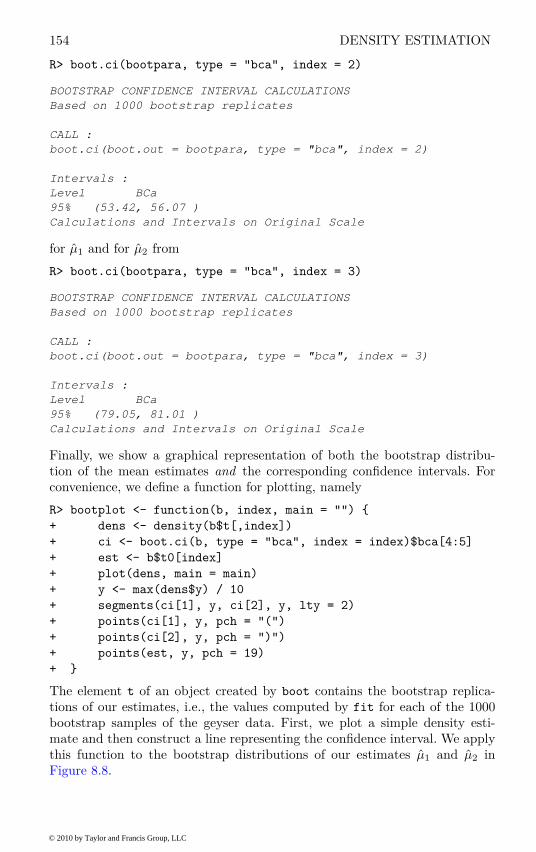
154 DENSITY ESTIMATION
R> boot.ci(bootpara, type = "bca", index = 2)
BOOTSTRAP CONFIDENCE INTERVAL CALCULATIONS
Based on 1000 bootstrap replicates
CALL :
boot.ci(boot.out = bootpara, type = "bca", index = 2)
Intervals :
Level BCa
95% (53.42, 56.07 )
Calculations and Intervals on Original Scale
for µ1 and for µ2 from
R> boot.ci(bootpara, type = "bca", index = 3)
BOOTSTRAP CONFIDENCE INTERVAL CALCULATIONS
Based on 1000 bootstrap replicates
CALL :
boot.ci(boot.out = bootpara, type = "bca", index = 3)
Intervals :
Level BCa
95% (79.05, 81.01 )
Calculations and Intervals on Original Scale
Finally, we show a graphical representation of both the bootstrap distribu-tion of the mean estimates and the corresponding confidence intervals. Forconvenience, we define a function for plotting, namely
R> bootplot <- function(b, index, main = "") {
+ dens <- density(b$t[,index])
+ ci <- boot.ci(b, type = "bca", index = index)$bca[4:5]
+ est <- b$t0[index]
+ plot(dens, main = main)
+ y <- max(dens$y) / 10
+ segments(ci[1], y, ci[2], y, lty = 2)
+ points(ci[1], y, pch = "(")
+ points(ci[2], y, pch = ")")
+ points(est, y, pch = 19)
+ }
The element t of an object created by boot contains the bootstrap replica-tions of our estimates, i.e., the values computed by fit for each of the 1000bootstrap samples of the geyser data. First, we plot a simple density esti-mate and then construct a line representing the confidence interval. We applythis function to the bootstrap distributions of our estimates µ1 and µ2 inFigure 8.8.
© 2010 by Taylor and Francis Group, LLC
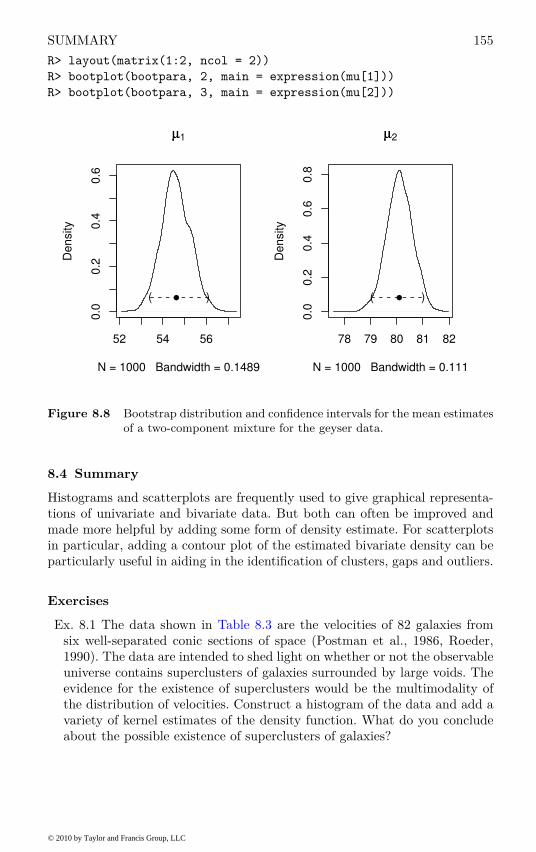
SUMMARY 155
R> layout(matrix(1:2, ncol = 2))
R> bootplot(bootpara, 2, main = expression(mu[1]))
R> bootplot(bootpara, 3, main = expression(mu[2]))
52 54 56
0.0
0.2
0.4
0.6
µµ1
N = 1000 Bandwidth = 0.1489
De
nsity
( )l
78 79 80 81 82
0.0
0.2
0.4
0.6
0.8
µµ2
N = 1000 Bandwidth = 0.111
De
nsity
( )l
Figure 8.8 Bootstrap distribution and confidence intervals for the mean estimates
of a two-component mixture for the geyser data.
8.4 Summary
Histograms and scatterplots are frequently used to give graphical representa-tions of univariate and bivariate data. But both can often be improved andmade more helpful by adding some form of density estimate. For scatterplotsin particular, adding a contour plot of the estimated bivariate density can beparticularly useful in aiding in the identification of clusters, gaps and outliers.
Exercises
Ex. 8.1 The data shown in Table 8.3 are the velocities of 82 galaxies fromsix well-separated conic sections of space (Postman et al., 1986, Roeder,1990). The data are intended to shed light on whether or not the observableuniverse contains superclusters of galaxies surrounded by large voids. Theevidence for the existence of superclusters would be the multimodality ofthe distribution of velocities. Construct a histogram of the data and add avariety of kernel estimates of the density function. What do you concludeabout the possible existence of superclusters of galaxies?
© 2010 by Taylor and Francis Group, LLC

156 DENSITY ESTIMATION
Table 8.3: galaxies data (package MASS). Velocities of 82galaxies.
galaxies galaxies galaxies galaxies galaxies
9172 19349 20196 22209 237069350 19440 20215 22242 237119483 19473 20221 22249 241299558 19529 20415 22314 242859775 19541 20629 22374 24289
10227 19547 20795 22495 2436610406 19663 20821 22746 2471716084 19846 20846 22747 2499016170 19856 20875 22888 2563318419 19863 20986 22914 2669018552 19914 21137 23206 2699518600 19918 21492 23241 3206518927 19973 21701 23263 3278919052 19989 21814 23484 3427919070 20166 21921 2353819330 20175 21960 2354219343 20179 22185 23666
Source: From Roeder, K., J. Am. Stat. Assoc., 85, 617–624, 1990. Reprintedwith permission from The Journal of the American Statistical Association.Copyright 1990 by the American Statistical Association. All rights reserved.
Ex. 8.2 The data in Table 8.4 give the birth and death rates for 69 countries(from Hartigan, 1975). Produce a scatterplot of the data that shows acontour plot of the estimated bivariate density. Does the plot give you anyinteresting insights into the possible structure of the data?
© 2010 by Taylor and Francis Group, LLC

SUMMARY 157
Table 8.4: birthdeathrates data. Birth and death rates for 69countries.
birth death birth death birth death
36.4 14.6 26.2 4.3 18.2 12.237.3 8.0 34.8 7.9 16.4 8.242.1 15.3 23.4 5.1 16.9 9.555.8 25.6 24.8 7.8 17.6 19.856.1 33.1 49.9 8.5 18.1 9.241.8 15.8 33.0 8.4 18.2 11.746.1 18.7 47.7 17.3 18.0 12.541.7 10.1 46.6 9.7 17.4 7.841.4 19.7 45.1 10.5 13.1 9.935.8 8.5 42.9 7.1 22.3 11.934.0 11.0 40.1 8.0 19.0 10.236.3 6.1 21.7 9.6 20.9 8.032.1 5.5 21.8 8.1 17.5 10.020.9 8.8 17.4 5.8 19.0 7.527.7 10.2 45.0 13.5 23.5 10.820.5 3.9 33.6 11.8 15.7 8.325.0 6.2 44.0 11.7 21.5 9.117.3 7.0 44.2 13.5 14.8 10.146.3 6.4 27.7 8.2 18.9 9.614.8 5.7 22.5 7.8 21.2 7.233.5 6.4 42.8 6.7 21.4 8.939.2 11.2 18.8 12.8 21.6 8.728.4 7.1 17.1 12.7 25.5 8.8
Source: From Hartigan, J. A., Clustering Algorithms, Wiley, New York,1975. With permission.
Ex. 8.3 A sex difference in the age of onset of schizophrenia was noted byKraepelin (1919). Subsequent epidemiological studies of the disorder haveconsistently shown an earlier onset in men than in women. One model thathas been suggested to explain this observed difference is known as the sub-
type model which postulates two types of schizophrenia, one characterisedby early onset, typical symptoms and poor premorbid competence, and theother by late onset, atypical symptoms and good premorbid competence.The early onset type is assumed to be largely a disorder of men and thelate onset largely a disorder of women. By fitting finite mixtures of normaldensities separately to the onset data for men and women given in Table 8.5see if you can produce some evidence for or against the subtype model.
© 2010 by Taylor and Francis Group, LLC
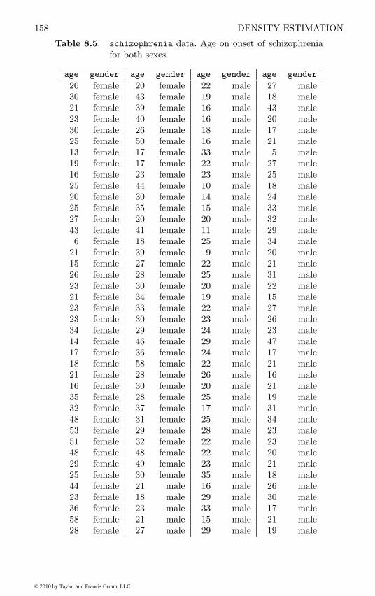
158 DENSITY ESTIMATION
Table 8.5: schizophrenia data. Age on onset of schizophreniafor both sexes.
age gender age gender age gender age gender
20 female 20 female 22 male 27 male30 female 43 female 19 male 18 male21 female 39 female 16 male 43 male23 female 40 female 16 male 20 male30 female 26 female 18 male 17 male25 female 50 female 16 male 21 male13 female 17 female 33 male 5 male19 female 17 female 22 male 27 male16 female 23 female 23 male 25 male25 female 44 female 10 male 18 male20 female 30 female 14 male 24 male25 female 35 female 15 male 33 male27 female 20 female 20 male 32 male43 female 41 female 11 male 29 male6 female 18 female 25 male 34 male
21 female 39 female 9 male 20 male15 female 27 female 22 male 21 male26 female 28 female 25 male 31 male23 female 30 female 20 male 22 male21 female 34 female 19 male 15 male23 female 33 female 22 male 27 male23 female 30 female 23 male 26 male34 female 29 female 24 male 23 male14 female 46 female 29 male 47 male17 female 36 female 24 male 17 male18 female 58 female 22 male 21 male21 female 28 female 26 male 16 male16 female 30 female 20 male 21 male35 female 28 female 25 male 19 male32 female 37 female 17 male 31 male48 female 31 female 25 male 34 male53 female 29 female 28 male 23 male51 female 32 female 22 male 23 male48 female 48 female 22 male 20 male29 female 49 female 23 male 21 male25 female 30 female 35 male 18 male44 female 21 male 16 male 26 male23 female 18 male 29 male 30 male36 female 23 male 33 male 17 male58 female 21 male 15 male 21 male28 female 27 male 29 male 19 male
© 2010 by Taylor and Francis Group, LLC
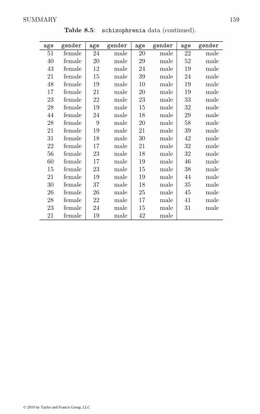
SUMMARY 159
Table 8.5: schizophrenia data (continued).
age gender age gender age gender age gender
51 female 24 male 20 male 22 male40 female 20 male 29 male 52 male43 female 12 male 24 male 19 male21 female 15 male 39 male 24 male48 female 19 male 10 male 19 male17 female 21 male 20 male 19 male23 female 22 male 23 male 33 male28 female 19 male 15 male 32 male44 female 24 male 18 male 29 male28 female 9 male 20 male 58 male21 female 19 male 21 male 39 male31 female 18 male 30 male 42 male22 female 17 male 21 male 32 male56 female 23 male 18 male 32 male60 female 17 male 19 male 46 male15 female 23 male 15 male 38 male21 female 19 male 19 male 44 male30 female 37 male 18 male 35 male26 female 26 male 25 male 45 male28 female 22 male 17 male 41 male23 female 24 male 15 male 31 male21 female 19 male 42 male
© 2010 by Taylor and Francis Group, LLC
CHAPTER 9
Recursive Partitioning: PredictingBody Fat and Glaucoma Diagnosis
9.1 Introduction
Worldwide, overweight and obesity are considered to be major health prob-lems because of their strong association with a higher risk of diseases of themetabolic syndrome, including diabetes mellitus and cardiovascular disease, aswell as with certain forms of cancer. Obesity is frequently evaluated by usingsimple indicators such as body mass index, waist circumference, or waist-to-hip ratio. Specificity and adequacy of these indicators are still controversial,mainly because they do not allow a precise assessment of body composition.Body fat, especially visceral fat, is suggested to be a better predictor of dis-eases of the metabolic syndrome. Garcia et al. (2005) report on the devel-opment of a multiple linear regression model for body fat content by meansof p = 9 common anthropometric measurements which were obtained forn = 71 healthy German women. In addition, the women’s body compositionwas measured by Dual Energy X-Ray Absorptiometry (DXA). This referencemethod is very accurate in measuring body fat but finds little applicability inpractical environments, mainly because of high costs and the methodologicalefforts needed. Therefore, a simple regression model for predicting DXA mea-surements of body fat is of special interest for the practitioner. The followingvariables are available (the measurements are given in Table 9.1):
DEXfat: body fat measured by DXA, the response variable,
age: age of the subject in years,
waistcirc: waist circumference,
hipcirc: hip circumference,
elbowbreadth: breadth of the elbow, and
kneebreadth: breadth of the knee.
Table 9.1: bodyfat data (package mboost). Body fat predic-tion by skinfold thickness, circumferences, and bonebreadths.
DEXfat age waistcirc hipcirc elbowbreadth kneebreadth
41.68 57 100.0 112.0 7.1 9.443.29 65 99.5 116.5 6.5 8.9
161
© 2010 by Taylor and Francis Group, LLC
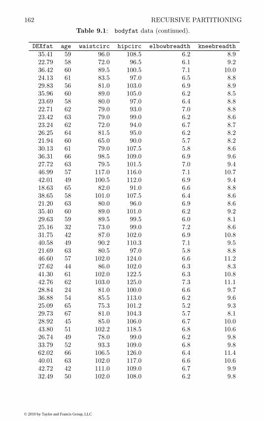
162 RECURSIVE PARTITIONING
Table 9.1: bodyfat data (continued).
DEXfat age waistcirc hipcirc elbowbreadth kneebreadth
35.41 59 96.0 108.5 6.2 8.922.79 58 72.0 96.5 6.1 9.236.42 60 89.5 100.5 7.1 10.024.13 61 83.5 97.0 6.5 8.829.83 56 81.0 103.0 6.9 8.935.96 60 89.0 105.0 6.2 8.523.69 58 80.0 97.0 6.4 8.822.71 62 79.0 93.0 7.0 8.823.42 63 79.0 99.0 6.2 8.623.24 62 72.0 94.0 6.7 8.726.25 64 81.5 95.0 6.2 8.221.94 60 65.0 90.0 5.7 8.230.13 61 79.0 107.5 5.8 8.636.31 66 98.5 109.0 6.9 9.627.72 63 79.5 101.5 7.0 9.446.99 57 117.0 116.0 7.1 10.742.01 49 100.5 112.0 6.9 9.418.63 65 82.0 91.0 6.6 8.838.65 58 101.0 107.5 6.4 8.621.20 63 80.0 96.0 6.9 8.635.40 60 89.0 101.0 6.2 9.229.63 59 89.5 99.5 6.0 8.125.16 32 73.0 99.0 7.2 8.631.75 42 87.0 102.0 6.9 10.840.58 49 90.2 110.3 7.1 9.521.69 63 80.5 97.0 5.8 8.846.60 57 102.0 124.0 6.6 11.227.62 44 86.0 102.0 6.3 8.341.30 61 102.0 122.5 6.3 10.842.76 62 103.0 125.0 7.3 11.128.84 24 81.0 100.0 6.6 9.736.88 54 85.5 113.0 6.2 9.625.09 65 75.3 101.2 5.2 9.329.73 67 81.0 104.3 5.7 8.128.92 45 85.0 106.0 6.7 10.043.80 51 102.2 118.5 6.8 10.626.74 49 78.0 99.0 6.2 9.833.79 52 93.3 109.0 6.8 9.862.02 66 106.5 126.0 6.4 11.440.01 63 102.0 117.0 6.6 10.642.72 42 111.0 109.0 6.7 9.932.49 50 102.0 108.0 6.2 9.8
© 2010 by Taylor and Francis Group, LLC
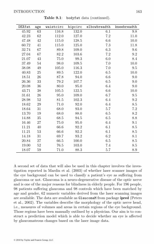
INTRODUCTION 163
Table 9.1: bodyfat data (continued).
DEXfat age waistcirc hipcirc elbowbreadth kneebreadth
45.92 63 116.8 132.0 6.1 9.842.23 62 112.0 127.0 7.2 11.047.48 42 115.0 128.5 6.6 10.060.72 41 115.0 125.0 7.3 11.832.74 67 89.8 109.0 6.3 9.627.04 67 82.2 103.6 7.2 9.221.07 43 75.0 99.3 6.0 8.437.49 54 98.0 109.5 7.0 10.038.08 49 105.0 116.3 7.0 9.540.83 25 89.5 122.0 6.5 10.018.51 26 87.8 94.0 6.6 9.026.36 33 79.2 107.7 6.5 9.020.08 36 80.0 95.0 6.4 9.043.71 38 105.5 122.5 6.6 10.031.61 26 95.0 109.0 6.7 9.528.98 52 81.5 102.3 6.4 9.218.62 29 71.0 92.0 6.4 8.518.64 31 68.0 93.0 5.7 7.213.70 19 68.0 88.0 6.5 8.214.88 35 68.5 94.5 6.5 8.816.46 27 75.0 95.0 6.4 9.111.21 40 66.6 92.2 6.1 8.511.21 53 66.6 92.2 6.1 8.514.18 31 69.7 93.2 6.2 8.120.84 27 66.5 100.0 6.5 8.519.00 52 76.5 103.0 7.4 8.518.07 59 71.0 88.3 5.7 8.9
A second set of data that will also be used in this chapter involves the inves-tigation reported in Mardin et al. (2003) of whether laser scanner images ofthe eye background can be used to classify a patient’s eye as suffering fromglaucoma or not. Glaucoma is a neuro-degenerative disease of the optic nerveand is one of the major reasons for blindness in elderly people. For 196 people,98 patients suffering glaucoma and 98 controls which have been matched byage and gender, 62 numeric variables derived from the laser scanning imagesare available. The data are available as GlaucomaM from package ipred (Peterset al., 2002). The variables describe the morphology of the optic nerve head,i.e., measures of volumes and areas in certain regions of the eye background.Those regions have been manually outlined by a physician. Our aim is to con-struct a prediction model which is able to decide whether an eye is affectedby glaucomateous changes based on the laser image data.
© 2010 by Taylor and Francis Group, LLC

164 RECURSIVE PARTITIONING
Both sets of data described above could be analysed using the regressionmodels described in Chapter 6 and Chapter 7, i.e., regression models for nu-meric and binary response variables based on a linear combination of thecovariates. But here we shall employ an alternative approach known as recur-
sive partitioning, where the resulting models are usually called regression or
classification trees. This method was originally invented to deal with possiblenon-linear relationships between covariates and response. The basic idea is topartition the covariate space and to compute simple statistics of the dependentvariable, like the mean or median, inside each cell.
9.2 Recursive Partitioning
There exist many algorithms for the construction of classification or regres-sion trees but the majority of algorithms follow a simple general rule: Firstpartition the observations by univariate splits in a recursive way and secondfit a constant model in each cell of the resulting partition. An overview of thisfield of regression models is given by Murthy (1998).
In more details, for the first step, one selects a covariate xj from the q
available covariates x1, . . . , xq and estimates a split point which separates theresponse values yi into two groups. For an ordered covariate xj a split point isa number ξ dividing the observations into two groups. The first group consistsof all observations with xj ≤ ξ and the second group contains the observationssatisfying xj > ξ. For a nominal covariate xj , the two groups are defined by aset of levels A where either xj ∈ A or xj 6∈ A.
Once the splits ξ or A for some selected covariate xj have been estimated,one applies the procedure sketched above for all observations in the first groupand, recursively, splits this set of observations further. The same happens forall observations in the second group. The recursion is stopped when somestopping criterion is fulfilled.
The available algorithms mostly differ with respect to three points: how thecovariate is selected in each step, how the split point is estimated and whichstopping criterion is applied. One of the most popular algorithms is describedin the Classification and Regression Trees book by Breiman et al. (1984) and isavailable in R by the functions in package rpart (Therneau and Atkinson, 1997,Therneau et al., 2009). This algorithm first examines all possible splits for allcovariates and chooses the split which leads to two groups that are ‘purer’ thanthe current group with respect to the values of the response variable y. Thereare many possible measures of impurity available, for regression problems withnominal response the Gini criterion is the default in rpart, alternatives anda more detailed description of tree based methods can be found in Ripley(1996).
The question when the recursion needs to stop is all but trivial. In fact,trees with too many leaves will suffer from overfitting and small trees willmiss important aspects of the problem. Commonly, this problem is addressedby so-called pruning methods. As the name suggests, one first grows a very
© 2010 by Taylor and Francis Group, LLC

ANALYSIS USING R 165
large tree using a trivial stopping criterion as the number of observations ina leaf, say, and then prunes branches that are not necessary.
Once that a tree has been grown, a simple summary statistic is computedfor each leaf. The mean or median can be used for continuous responses andfor nominal responses the proportions of the classes is commonly used. Theprediction of a new observation is simply the corresponding summary statisticof the leaf to which this observation belongs.
However, even the right-sized tree consists of binary splits which are, ofcourse, hard decisions. When the underlying relationship between covariateand response is smooth, such a split point estimate will be affected by highvariability. This problem is addressed by so called ensemble methods. Here,multiple trees are grown on perturbed instances of the data set and theirpredictions are averaged. The simplest representative of such a procedure iscalled bagging (Breiman, 1996) and works as follows. We draw B bootstrapsamples from the original data set, i.e., we draw n out of n observations withreplacement from our n original observations. For each of those bootstrapsamples we grow a very large tree. When we are interested in the predictionfor a new observation, we pass this observation through all B trees and averagetheir predictions. It has been shown that the goodness of the predictions forfuture cases can be improved dramatically by this or similar simple procedures.More details can be found in Buhlmann (2004).
9.3 Analysis Using R
9.3.1 Predicting Body Fat Content
The rpart function from rpart can be used to grow a regression tree. Theresponse variable and the covariates are defined by a model formula in thesame way as for lm, say. By default, a large initial tree is grown, we restrictthe number of observations required to establish a potential binary split to atleast ten:
R> library("rpart")
R> data("bodyfat", package = "mboost")
R> bodyfat_rpart <- rpart(DEXfat ~ age + waistcirc + hipcirc +
+ elbowbreadth + kneebreadth, data = bodyfat,
+ control = rpart.control(minsplit = 10))
A print method for rpart objects is available; however, a graphical repre-sentation (here utilising functionality offered from package partykit, Hothornand Zeileis, 2009) shown in Figure 9.1 is more convenient. Observations thatsatisfy the condition shown for each node go to the left and observations thatdon’t are element of the right branch in each node. As expected, higher valuesfor waist- and hip circumferences and wider knees correspond to higher valuesof body fat content. The rightmost terminal node consists of only three ratherextreme observations.
© 2010 by Taylor and Francis Group, LLC
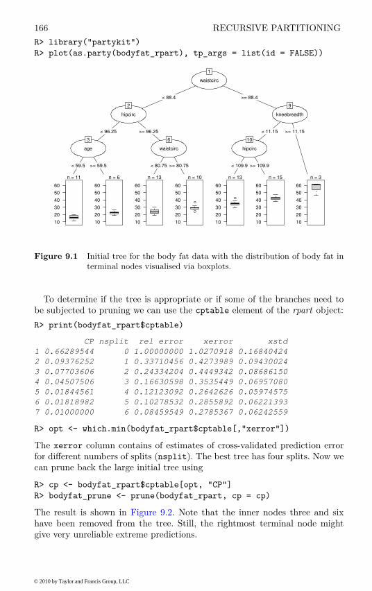
166 RECURSIVE PARTITIONING
R> library("partykit")
R> plot(as.party(bodyfat_rpart), tp_args = list(id = FALSE))
waistcirc
1
< 88.4 >= 88.4
hipcirc
2
< 96.25 >= 96.25
age
3
< 59.5 >= 59.5
n = 11
10
20
30
40
50
60
n = 6
10
20
30
40
50
60
waistcirc
6
< 80.75 >= 80.75
n = 13
10
20
30
40
50
60
n = 10
10
20
30
40
50
60
kneebreadth
9
< 11.15 >= 11.15
hipcirc
10
< 109.9 >= 109.9
n = 13
10
20
30
40
50
60
n = 15
10
20
30
40
50
60
n = 3
10
20
30
40
50
60
Figure 9.1 Initial tree for the body fat data with the distribution of body fat interminal nodes visualised via boxplots.
To determine if the tree is appropriate or if some of the branches need tobe subjected to pruning we can use the cptable element of the rpart object:
R> print(bodyfat_rpart$cptable)
CP nsplit rel error xerror xstd
1 0.66289544 0 1.00000000 1.0270918 0.16840424
2 0.09376252 1 0.33710456 0.4273989 0.09430024
3 0.07703606 2 0.24334204 0.4449342 0.08686150
4 0.04507506 3 0.16630598 0.3535449 0.06957080
5 0.01844561 4 0.12123092 0.2642626 0.05974575
6 0.01818982 5 0.10278532 0.2855892 0.06221393
7 0.01000000 6 0.08459549 0.2785367 0.06242559
R> opt <- which.min(bodyfat_rpart$cptable[,"xerror"])
The xerror column contains of estimates of cross-validated prediction errorfor different numbers of splits (nsplit). The best tree has four splits. Now wecan prune back the large initial tree using
R> cp <- bodyfat_rpart$cptable[opt, "CP"]
R> bodyfat_prune <- prune(bodyfat_rpart, cp = cp)
The result is shown in Figure 9.2. Note that the inner nodes three and sixhave been removed from the tree. Still, the rightmost terminal node mightgive very unreliable extreme predictions.
© 2010 by Taylor and Francis Group, LLC
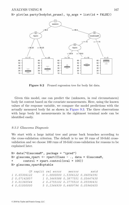
ANALYSIS USING R 167
R> plot(as.party(bodyfat_prune), tp_args = list(id = FALSE))
waistcirc
1
< 88.4 >= 88.4
hipcirc
2
< 96.25 >= 96.25
n = 17
10
20
30
40
50
60
n = 23
10
20
30
40
50
60
kneebreadth
5
< 11.15 >= 11.15
hipcirc
6
< 109.9 >= 109.9
n = 13
10
20
30
40
50
60
n = 15
10
20
30
40
50
60
n = 3
10
20
30
40
50
60
Figure 9.2 Pruned regression tree for body fat data.
Given this model, one can predict the (unknown, in real circumstances)body fat content based on the covariate measurements. Here, using the knownvalues of the response variable, we compare the model predictions with theactually measured body fat as shown in Figure 9.3. The three observationswith large body fat measurements in the rightmost terminal node can beidentified easily.
9.3.2 Glaucoma Diagnosis
We start with a large initial tree and prune back branches according tothe cross-validation criterion. The default is to use 10 runs of 10-fold cross-validation and we choose 100 runs of 10-fold cross-validation for reasons to beexplained later.
R> data("GlaucomaM", package = "ipred")
R> glaucoma_rpart <- rpart(Class ~ ., data = GlaucomaM,
+ control = rpart.control(xval = 100))
R> glaucoma_rpart$cptable
CP nsplit rel error xerror xstd
1 0.65306122 0 1.0000000 1.5306122 0.06054391
2 0.07142857 1 0.3469388 0.3877551 0.05647630
3 0.01360544 2 0.2755102 0.3775510 0.05590431
4 0.01000000 5 0.2346939 0.4489796 0.05960655
© 2010 by Taylor and Francis Group, LLC
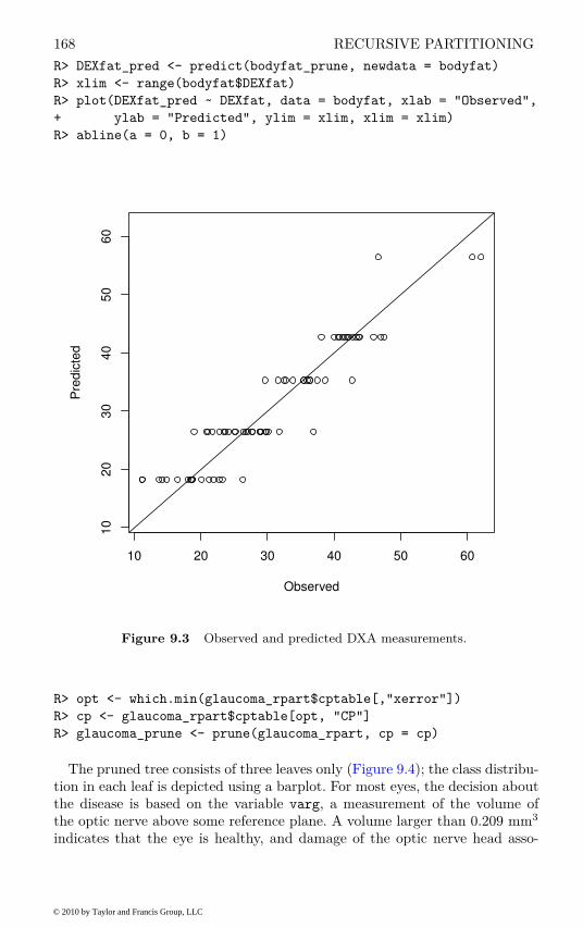
168 RECURSIVE PARTITIONING
R> DEXfat_pred <- predict(bodyfat_prune, newdata = bodyfat)
R> xlim <- range(bodyfat$DEXfat)
R> plot(DEXfat_pred ~ DEXfat, data = bodyfat, xlab = "Observed",
+ ylab = "Predicted", ylim = xlim, xlim = xlim)
R> abline(a = 0, b = 1)
10 20 30 40 50 60
10
20
30
40
50
60
Observed
Pre
dic
ted
Figure 9.3 Observed and predicted DXA measurements.
R> opt <- which.min(glaucoma_rpart$cptable[,"xerror"])
R> cp <- glaucoma_rpart$cptable[opt, "CP"]
R> glaucoma_prune <- prune(glaucoma_rpart, cp = cp)
The pruned tree consists of three leaves only (Figure 9.4); the class distribu-tion in each leaf is depicted using a barplot. For most eyes, the decision aboutthe disease is based on the variable varg, a measurement of the volume ofthe optic nerve above some reference plane. A volume larger than 0.209 mm3
indicates that the eye is healthy, and damage of the optic nerve head asso-
© 2010 by Taylor and Francis Group, LLC
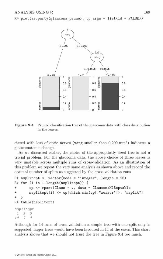
ANALYSIS USING R 169
R> plot(as.party(glaucoma_prune), tp_args = list(id = FALSE))
varg
1
< 0.209 >= 0.209
n = 76
no
rma
lg
lau
co
ma
0
0.2
0.4
0.6
0.8
1
mhcg
3
>= 0.1695 < 0.1695
n = 7
no
rma
lg
lau
co
ma
0
0.2
0.4
0.6
0.8
1n = 113
no
rma
lg
lau
co
ma
0
0.2
0.4
0.6
0.8
1
Figure 9.4 Pruned classification tree of the glaucoma data with class distributionin the leaves.
ciated with loss of optic nerves (varg smaller than 0.209 mm3) indicates aglaucomateous change.
As we discussed earlier, the choice of the appropriatly sized tree is not atrivial problem. For the glaucoma data, the above choice of three leaves isvery unstable across multiple runs of cross-validation. As an illustration ofthis problem we repeat the very same analysis as shown above and record theoptimal number of splits as suggested by the cross-validation runs.
R> nsplitopt <- vector(mode = "integer", length = 25)
R> for (i in 1:length(nsplitopt)) {
+ cp <- rpart(Class ~ ., data = GlaucomaM)$cptable
+ nsplitopt[i] <- cp[which.min(cp[,"xerror"]), "nsplit"]
+ }
R> table(nsplitopt)
nsplitopt
1 2 5
14 7 4
Although for 14 runs of cross-validation a simple tree with one split only issuggested, larger trees would have been favoured in 11 of the cases. This shortanalysis shows that we should not trust the tree in Figure 9.4 too much.
© 2010 by Taylor and Francis Group, LLC

170 RECURSIVE PARTITIONING
One way out of this dilemma is the aggregation of multiple trees via bagging.In R, the bagging idea can be implemented by three or four lines of code. Casecount or weight vectors representing the bootstrap samples can be drawn fromthe multinominal distribution with parameters n and p1 = 1/n, . . . , pn =1/n via the rmultinom function. For each weight vector, one large tree isconstructed without pruning and the rpart objects are stored in a list, herecalled trees:
R> trees <- vector(mode = "list", length = 25)
R> n <- nrow(GlaucomaM)
R> bootsamples <- rmultinom(length(trees), n, rep(1, n)/n)
R> mod <- rpart(Class ~ ., data = GlaucomaM,
+ control = rpart.control(xval = 0))
R> for (i in 1:length(trees))
+ trees[[i]] <- update(mod, weights = bootsamples[,i])
The update function re-evaluates the call of mod, however, with the weightsbeing altered, i.e., fits a tree to a bootstrap sample specified by the weights.It is interesting to have a look at the structures of the multiple trees. Forexample, the variable selected for splitting in the root of the tree is not uniqueas can be seen by
R> table(sapply(trees, function(x) as.character(x$frame$var[1])))
phcg varg vari vars
1 14 9 1
Although varg is selected most of the time, other variables such as vari occuras well – a further indication that the tree in Figure 9.4 is questionable andthat hard decisions are not appropriate for the glaucoma data.
In order to make use of the ensemble of trees in the list trees we estimatethe conditional probability of suffering from glaucoma given the covariates foreach observation in the original data set by
R> classprob <- matrix(0, nrow = n, ncol = length(trees))
R> for (i in 1:length(trees)) {
+ classprob[,i] <- predict(trees[[i]],
+ newdata = GlaucomaM)[,1]
+ classprob[bootsamples[,i] > 0,i] <- NA
+ }
Thus, for each observation we get 25 estimates. However, each observation hasbeen used for growing one of the trees with probability 0.632 and thus wasnot used with probability 0.368. Consequently, the estimate from a tree wherean observation was not used for growing is better for judging the quality ofthe predictions and we label the other estimates with NA.
Now, we can average the estimates and we vote for glaucoma when theaverage of the estimates of the conditional glaucoma probability exceeds 0.5.The comparison between the observed and the predicted classes does not sufferfrom overfitting since the predictions are computed from those trees for whicheach single observation was not used for growing.
© 2010 by Taylor and Francis Group, LLC

ANALYSIS USING R 171
R> avg <- rowMeans(classprob, na.rm = TRUE)
R> predictions <- factor(ifelse(avg > 0.5, "glaucoma",
+ "normal"))
R> predtab <- table(predictions, GlaucomaM$Class)
R> predtab
predictions glaucoma normal
glaucoma 77 16
normal 21 82
Thus, an honest estimate of the probability of a glaucoma prediction whenthe patient is actually suffering from glaucoma is
R> round(predtab[1,1] / colSums(predtab)[1] * 100)
glaucoma
79
per cent. For
R> round(predtab[2,2] / colSums(predtab)[2] * 100)
normal
84
per cent of normal eyes, the ensemble does not predict a glaucomateous dam-age.
Although we are mainly interested in a predictor, i.e., a black box machinefor predicting glaucoma is our main focus, the nature of the black box mightbe interesting as well. From the classification tree analysis shown above weexpect to see a relationship between the volume above the reference plane(varg) and the estimated conditional probability of suffering from glaucoma.A graphical approach is sufficient here and we simply plot the observed valuesof varg against the averages of the estimated glaucoma probability (such plotshave been used by Breiman, 2001b, Garczarek and Weihs, 2003, for example).In addition, we construct such a plot for another covariate as well, namelyvari, the volume above the reference plane measured in the inferior part ofthe optic nerve head only. Figure 9.5 shows that the initial split of 0.209mm
3
for varg (see Figure 9.4) corresponds to the ensemble predictions rather well.The bagging procedure is a special case of a more general approach called
random forest (Breiman, 2001a). The package randomForest (Breiman et al.,2009) can be used to compute such ensembles via
R> library("randomForest")
R> rf <- randomForest(Class ~ ., data = GlaucomaM)
and we obtain out-of-bag estimates for the prediction error via
R> table(predict(rf), GlaucomaM$Class)
glaucoma normal
glaucoma 80 12
normal 18 86
© 2010 by Taylor and Francis Group, LLC
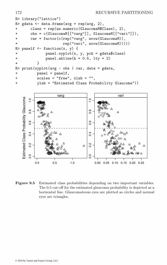
172 RECURSIVE PARTITIONING
R> library("lattice")
R> gdata <- data.frame(avg = rep(avg, 2),
+ class = rep(as.numeric(GlaucomaM$Class), 2),
+ obs = c(GlaucomaM[["varg"]], GlaucomaM[["vari"]]),
+ var = factor(c(rep("varg", nrow(GlaucomaM)),
+ rep("vari", nrow(GlaucomaM)))))
R> panelf <- function(x, y) {
+ panel.xyplot(x, y, pch = gdata$class)
+ panel.abline(h = 0.5, lty = 2)
+ }
R> print(xyplot(avg ~ obs | var, data = gdata,
+ panel = panelf,
+ scales = "free", xlab = "",
+ ylab = "Estimated Class Probability Glaucoma"))
Estim
ate
d C
lass P
rob
ab
ility
Gla
uco
ma
0.0
0.2
0.4
0.6
0.8
1.0
0.0 0.5 1.0
varg
0.0
0.2
0.4
0.6
0.8
1.0
0.00 0.05 0.10 0.15 0.20 0.25
vari
Figure 9.5 Estimated class probabilities depending on two important variables.The 0.5 cut-off for the estimated glaucoma probability is depicted as ahorizontal line. Glaucomateous eyes are plotted as circles and normaleyes are triangles.
© 2010 by Taylor and Francis Group, LLC

ANALYSIS USING R 173
R> plot(bodyfat_ctree)
hipcircp < 0.001
1
≤≤ 108 >> 108
waistcircp < 0.001
2
≤≤ 76.5 >> 76.5
Node 3 (n = 17)
10
20
30
40
50
60
hipcircp < 0.001
4
≤≤ 99 >> 99
Node 5 (n = 11)
10
20
30
40
50
60
Node 6 (n = 17)
10
20
30
40
50
60
kneebreadthp = 0.003
7
≤≤ 10 >> 10
Node 8 (n = 17)
10
20
30
40
50
60
Node 9 (n = 9)
10
20
30
40
50
60
Figure 9.6 Conditional inference tree with the distribution of body fat contentshown for each terminal leaf.
9.3.3 Trees Revisited
Another approach to recursive partitioning, making a connection to classicalstatistical test problems such as those discussed in Chapter 4, is implementedin the party package (Hothorn et al., 2006b, 2009c). In each node of thosetrees, a significance test on independence between any of the covariates andthe response is performed and a split is established when the p-value, possiblyadjusted for multiple comparisons, is smaller than a pre-specified nominal levelα. This approach has the advantage that one does not need to prune backlarge initial trees since we have a statistically motivated stopping criterion –the p-value – at hand.
For the body fat data, such a conditional inference tree can be computedusing the ctree function
R> library("party")
R> bodyfat_ctree <- ctree(DEXfat ~ age + waistcirc + hipcirc +
+ elbowbreadth + kneebreadth, data = bodyfat)
This tree doesn’t require a pruning procedure because an internal stop crite-rion based on formal statistical tests prevents the procedure from overfittingthe data. The tree structure is shown in Figure 9.6. Although the structureof this tree and the tree depicted in Figure 9.2 are rather different, the corre-sponding predictions don’t vary too much.
Very much the same code is needed to grow a tree on the glaucoma data:
R> glaucoma_ctree <- ctree(Class ~ ., data = GlaucomaM)
© 2010 by Taylor and Francis Group, LLC
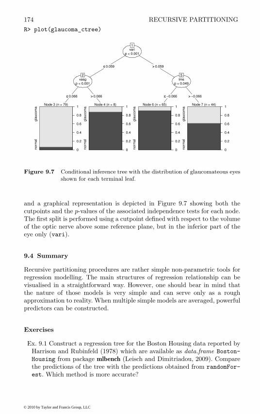
174 RECURSIVE PARTITIONING
R> plot(glaucoma_ctree)
varip < 0.001
1
≤≤ 0.059 >> 0.059
vasgp < 0.001
2
≤≤ 0.066 >> 0.066
Node 3 (n = 79)
no
rma
lg
lau
co
ma
0
0.2
0.4
0.6
0.8
1Node 4 (n = 8)
no
rma
lg
lau
co
ma
0
0.2
0.4
0.6
0.8
1
tmsp = 0.049
5
≤≤ −0.066 >> −0.066
Node 6 (n = 65)
no
rma
lg
lau
co
ma
0
0.2
0.4
0.6
0.8
1Node 7 (n = 44)
no
rma
lg
lau
co
ma
0
0.2
0.4
0.6
0.8
1
Figure 9.7 Conditional inference tree with the distribution of glaucomateous eyesshown for each terminal leaf.
and a graphical representation is depicted in Figure 9.7 showing both thecutpoints and the p-values of the associated independence tests for each node.The first split is performed using a cutpoint defined with respect to the volumeof the optic nerve above some reference plane, but in the inferior part of theeye only (vari).
9.4 Summary
Recursive partitioning procedures are rather simple non-parametric tools forregression modelling. The main structures of regression relationship can bevisualised in a straightforward way. However, one should bear in mind thatthe nature of those models is very simple and can serve only as a roughapproximation to reality. When multiple simple models are averaged, powerfulpredictors can be constructed.
Exercises
Ex. 9.1 Construct a regression tree for the Boston Housing data reported byHarrison and Rubinfeld (1978) which are available as data.frame Boston-
Housing from package mlbench (Leisch and Dimitriadou, 2009). Comparethe predictions of the tree with the predictions obtained from randomFor-
est. Which method is more accurate?
© 2010 by Taylor and Francis Group, LLC

SUMMARY 175
Ex. 9.2 For each possible cutpoint in varg of the glaucoma data, computethe test statistic of the chi-square test of independence (see Chapter 3) andplot them against the values of varg. Is a simple cutpoint for this variableappropriate for discriminating between healthy and glaucomateous eyes?
Ex. 9.3 Compare the tree models fitted to the glaucoma data with a logisticregression model (see Chapter 7).
© 2010 by Taylor and Francis Group, LLC

CHAPTER 10
Scatterplot Smoothers and GeneralisedAdditive Models: The Men’s Olympic1500m, Air Pollution in the USA, and
Risk Factors for Kyphosis
10.1 Introduction
The modern Olympics began in 1896 in Greece and have been held every fouryears since, apart from interruptions due to the two world wars. On the trackthe blue ribbon event has always been the 1500m for men since competitorsthat want to win must have a unique combination of speed, strength andstamina combined with an acute tactical awareness. For the spectator theevent lasts long enough to be interesting (unlike say the 100m dash) but nottoo long so as to become boring (as do most 10,000m races). The event hasbeen witness to some of the most dramatic scenes in Olympic history; whocan forget Herb Elliott winning by a street in 1960, breaking the world recordand continuing his sequence of never being beaten in a 1500m or mile race inhis career? And remembering the joy and relief etched on the face of Seb Coewhen winning and beating his arch rival Steve Ovett still brings a tear to theeye of many of us.
The complete record of winners of the men’s 1500m from 1896 to 2004 isgiven in Table 10.1. Can we use these winning times as the basis of a suitablestatistical model that will enable us to predict the winning times for futureOlympics?
Table 10.1: men1500m data. Olympic Games 1896 to 2004 win-ners of the men’s 1500m.
year venue winner country time
1896 Athens E. Flack Australia 273.201900 Paris C. Bennett Great Britain 246.201904 St. Louis J. Lightbody USA 245.401908 London M. Sheppard USA 243.401912 Stockholm A. Jackson Great Britain 236.801920 Antwerp A. Hill Great Britain 241.801924 Paris P. Nurmi Finland 233.601928 Amsterdam H. Larva Finland 233.201932 Los Angeles L. Beccali Italy 231.20
177
© 2010 by Taylor and Francis Group, LLC

178 SMOOTHERS AND GENERALISED ADDITIVE MODELS
Table 10.1: men1500m data (continued).
year venue winner country time
1936 Berlin J. Lovelock New Zealand 227.801948 London H. Eriksson Sweden 229.801952 Helsinki J. Barthel Luxemborg 225.101956 Melbourne R. Delaney Ireland 221.201960 Rome H. Elliott Australia 215.601964 Tokyo P. Snell New Zealand 218.101968 Mexico City K. Keino Kenya 214.901972 Munich P. Vasala Finland 216.301976 Montreal J. Walker New Zealand 219.171980 Moscow S. Coe Great Britain 218.401984 Los Angeles S. Coe Great Britain 212.531988 Seoul P. Rono Kenya 215.951992 Barcelona F. Cacho Spain 220.121996 Atlanta N. Morceli Algeria 215.782000 Sydney K. Ngenyi Kenya 212.072004 Athens H. El Guerrouj Morocco 214.18
The data in Table 10.2 relate to air pollution in 41 US cities as reported bySokal and Rohlf (1981). The annual mean concentration of sulphur dioxide,in micrograms per cubic metre, is a measure of the air pollution of the city.The question of interest here is what aspects of climate and human ecologyas measured by the other six variables in the table determine pollution. Thus,we are interested in a regression model from which we can infer the relation-ship between each of the exploratory variables to the response (SO2 content).Details of the seven measurements are;
SO2: SO2 content of air in micrograms per cubic metre,
temp: average annual temperature in Fahrenheit,
manu: number of manufacturing enterprises employing 20 or more workers,
popul: population size (1970 census); in thousands,
wind: average annual wind speed in miles per hour,
precip: average annual precipitation in inches,
predays: average number of days with precipitation per year.
Table 10.2: USairpollution data. Air pollution in 41 US cities.
SO2 temp manu popul wind precip predays
Albany 46 47.6 44 116 8.8 33.36 135Albuquerque 11 56.8 46 244 8.9 7.77 58
© 2010 by Taylor and Francis Group, LLC

INTRODUCTION 179
Table 10.2: USairpollution data (continued).
SO2 temp manu popul wind precip predays
Atlanta 24 61.5 368 497 9.1 48.34 115Baltimore 47 55.0 625 905 9.6 41.31 111Buffalo 11 47.1 391 463 12.4 36.11 166Charleston 31 55.2 35 71 6.5 40.75 148Chicago 110 50.6 3344 3369 10.4 34.44 122Cincinnati 23 54.0 462 453 7.1 39.04 132Cleveland 65 49.7 1007 751 10.9 34.99 155Columbus 26 51.5 266 540 8.6 37.01 134Dallas 9 66.2 641 844 10.9 35.94 78Denver 17 51.9 454 515 9.0 12.95 86Des Moines 17 49.0 104 201 11.2 30.85 103Detroit 35 49.9 1064 1513 10.1 30.96 129Hartford 56 49.1 412 158 9.0 43.37 127Houston 10 68.9 721 1233 10.8 48.19 103Indianapolis 28 52.3 361 746 9.7 38.74 121Jacksonville 14 68.4 136 529 8.8 54.47 116Kansas City 14 54.5 381 507 10.0 37.00 99Little Rock 13 61.0 91 132 8.2 48.52 100Louisville 30 55.6 291 593 8.3 43.11 123Memphis 10 61.6 337 624 9.2 49.10 105Miami 10 75.5 207 335 9.0 59.80 128Milwaukee 16 45.7 569 717 11.8 29.07 123Minneapolis 29 43.5 699 744 10.6 25.94 137Nashville 18 59.4 275 448 7.9 46.00 119New Orleans 9 68.3 204 361 8.4 56.77 113Norfolk 31 59.3 96 308 10.6 44.68 116Omaha 14 51.5 181 347 10.9 30.18 98Philadelphia 69 54.6 1692 1950 9.6 39.93 115Phoenix 10 70.3 213 582 6.0 7.05 36Pittsburgh 61 50.4 347 520 9.4 36.22 147Providence 94 50.0 343 179 10.6 42.75 125Richmond 26 57.8 197 299 7.6 42.59 115Salt Lake City 28 51.0 137 176 8.7 15.17 89San Francisco 12 56.7 453 716 8.7 20.66 67Seattle 29 51.1 379 531 9.4 38.79 164St. Louis 56 55.9 775 622 9.5 35.89 105Washington 29 57.3 434 757 9.3 38.89 111Wichita 8 56.6 125 277 12.7 30.58 82Wilmington 36 54.0 80 80 9.0 40.25 114
Source: From Sokal, R. R., Rohlf, F. J., Biometry, W. H. Freeman, San Fran-cisco, USA, 1981. With permission.
© 2010 by Taylor and Francis Group, LLC
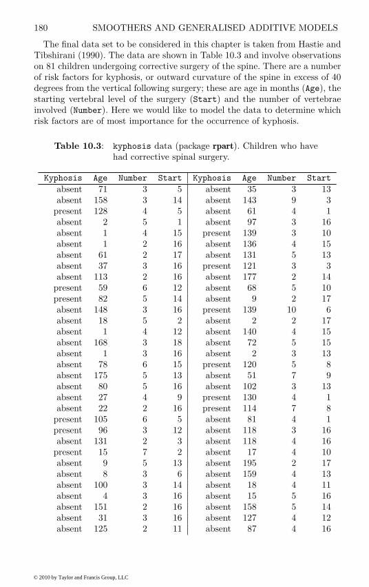
180 SMOOTHERS AND GENERALISED ADDITIVE MODELS
The final data set to be considered in this chapter is taken from Hastie andTibshirani (1990). The data are shown in Table 10.3 and involve observationson 81 children undergoing corrective surgery of the spine. There are a numberof risk factors for kyphosis, or outward curvature of the spine in excess of 40degrees from the vertical following surgery; these are age in months (Age), thestarting vertebral level of the surgery (Start) and the number of vertebraeinvolved (Number). Here we would like to model the data to determine whichrisk factors are of most importance for the occurrence of kyphosis.
Table 10.3: kyphosis data (package rpart). Children who havehad corrective spinal surgery.
Kyphosis Age Number Start Kyphosis Age Number Start
absent 71 3 5 absent 35 3 13absent 158 3 14 absent 143 9 3
present 128 4 5 absent 61 4 1absent 2 5 1 absent 97 3 16absent 1 4 15 present 139 3 10absent 1 2 16 absent 136 4 15absent 61 2 17 absent 131 5 13absent 37 3 16 present 121 3 3absent 113 2 16 absent 177 2 14
present 59 6 12 absent 68 5 10present 82 5 14 absent 9 2 17absent 148 3 16 present 139 10 6absent 18 5 2 absent 2 2 17absent 1 4 12 absent 140 4 15absent 168 3 18 absent 72 5 15absent 1 3 16 absent 2 3 13absent 78 6 15 present 120 5 8absent 175 5 13 absent 51 7 9absent 80 5 16 absent 102 3 13absent 27 4 9 present 130 4 1absent 22 2 16 present 114 7 8
present 105 6 5 absent 81 4 1present 96 3 12 absent 118 3 16absent 131 2 3 absent 118 4 16
present 15 7 2 absent 17 4 10absent 9 5 13 absent 195 2 17absent 8 3 6 absent 159 4 13absent 100 3 14 absent 18 4 11absent 4 3 16 absent 15 5 16absent 151 2 16 absent 158 5 14absent 31 3 16 absent 127 4 12absent 125 2 11 absent 87 4 16
© 2010 by Taylor and Francis Group, LLC

SMOOTHERS AND GENERALISED ADDITIVE MODELS 181
Table 10.3: kyphosis data (continued).
Kyphosis Age Number Start Kyphosis Age Number Start
absent 130 5 13 absent 206 4 10absent 112 3 16 absent 11 3 15absent 140 5 11 absent 178 4 15absent 93 3 16 present 157 3 13absent 1 3 9 absent 26 7 13
present 52 5 6 absent 120 2 13absent 20 6 9 present 42 7 6
present 91 5 12 absent 36 4 13present 73 5 1
10.2 Scatterplot Smoothers and Generalised Additive Models
Each of the three data sets described in the Introduction appear to be perfectcandidates to be analysed by one of the methods described in earlier chapters.Simple linear regression could, for example, be applied to the 1500m timesand multiple linear regression to the pollution data; the kyphosis data couldbe analysed using logistic regression. But instead of assuming we know thelinear functional form for a regression model we might consider an alterna-tive approach in which the appropriate functional form is estimated from thedata. How is this achieved? The secret is to replace the global estimates fromthe regression models considered in earlier chapters with local estimates, inwhich the statistical dependency between two variables is described, not witha single parameter such as a regression coefficient, but with a series of lo-cal estimates. For example, a regression might be estimated between the twovariables for some restricted range of values for each variable and the pro-cess repeated across the range of each variable. The series of local estimatesis then aggregated by drawing a line to summarise the relationship betweenthe two variables. In this way no particular functional form is imposed on therelationship. Such an approach is particularly useful when
• the relationship between the variables is expected to be of a complex form,not easily fitted by standard linear or nonlinear models;
• there is no a priori reason for using a particular model;
• we would like the data themselves to suggest the appropriate functionalform.
The starting point for a local estimation approach to fitting relationshipsbetween variables is scatterplot smoothers, which are described in the nextsubsection.
© 2010 by Taylor and Francis Group, LLC

182 SMOOTHERS AND GENERALISED ADDITIVE MODELS
10.2.1 Scatterplot Smoothers
The scatterplot is an excellent first exploratory graph to study the dependenceof two variables and all readers will be familiar with plotting the outcome ofa simple linear regression fit onto the graph to help in a better understand-ing of the pattern of dependence. But many readers will probably be lessfamiliar with some non-parametric alternatives to linear regression fits thatmay be more useful than the latter in many situations. These alternativesare labelled non-parametric since unlike parametric techniques such as lin-ear regression they do not summarise the relationship between two variableswith a parameter such as a regression or correlation coefficient. Instead non-parametric ‘smoothers’ summarise the relationship between two variables witha line drawing. The simplest of this collection of non-parametric smoothers is alocally weighted regression or lowess fit, first suggested by Cleveland (1979). Inessence this approach assumes that the independent variable xi and a responseyi are related by
yi = g(xi) + εi, i = 1, . . . , n
where g is a locally defined p-degree polynomial function in the predictorvariable, xi, and εi are random variables with mean zero and constant scale.Values yi = g(xi) are used to estimate the yi at each xi and are found byfitting the polynomials using weighted least squares with large weights forpoints near to xi and small otherwise. Two parameters control the shape of alowess curve; the first is a smoothing parameter, α, (often know as the span,the width of the local neighbourhood) with larger values leading to smoothercurves – typical values are 0.25 to 1. In essence the span decides the amountof the tradeoff between reduction in bias and increase in variance. If the spanis too large, the non-parametric regression estimate will be biased, but if thespan is too small, the estimate will be overfitted with inflated variance. Keele(2008) gives an extended discussion of the influence of the choice of span onthe non-parametric regression. The second parameter, λ , is the degree of thepolynomials that are fitted by the method; λ can be 0, 1, or 2. In any specificapplication, the change of the two parameters must be based on a combinationof judgement and of trial and error. Residual plots may be helpful in judginga particular combination of values.
An alternative smoother that can often be usefully applied to bivariate datais some form of spline function. (A spline is a term for a flexible strip of metal orrubber used by a draftsman to draw curves.) Spline functions are polynomialswithin intervals of the x-variable that are smoothly connected across differentvalues of x. Figure 10.1 for example shows a linear spline function, i.e., apiecewise linear function, of the form
f(x) = β0 + β1x + β2(x − a)+ + β3(x − b)+ + β4(x − c)+
where (u)+ = u for u > 0 and zero otherwise. The interval endpoints, a, b, andc, are called knots. The number of knots can vary according to the amount ofdata available for fitting the function.
© 2010 by Taylor and Francis Group, LLC
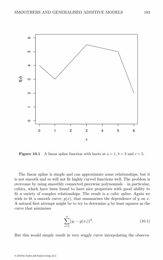
SMOOTHERS AND GENERALISED ADDITIVE MODELS 183
0 1 2 3 4 5 6
01
23
45
6
x
f((x))
Figure 10.1 A linear spline function with knots at a = 1, b = 3 and c = 5.
The linear spline is simple and can approximate some relationships, but itis not smooth and so will not fit highly curved functions well. The problem isovercome by using smoothly connected piecewise polynomials – in particular,cubics, which have been found to have nice properties with good ability tofit a variety of complex relationships. The result is a cubic spline. Again wewish to fit a smooth curve, g(x), that summarises the dependence of y on x.A natural first attempt might be to try to determine g by least squares as thecurve that minimises
n∑
i=1
(yi − g(xi))2. (10.1)
But this would simply result in very wiggly curve interpolating the observa-
© 2010 by Taylor and Francis Group, LLC

184 SMOOTHERS AND GENERALISED ADDITIVE MODELS
tions. Instead of (10.1) the criterion used to determine g is
n∑
i=1
(yi − g(xi))2 + λ
∫
g′′(x)2 dx (10.2)
where g′′(x) represents the second derivation of g(x) with respect to x. Al-though written formally this criterion looks a little formidable, it is reallynothing more than an effort to govern the trade-off between the goodness-of-fit of the data (as measured by
∑
(yi − g(xi))2 ) and the ‘wiggliness’ or
departure of linearity of g measured by∫
g′′(x)2 dx; for a linear function, thispart of (10.2) would be zero. The parameter λ governs the smoothness of g,with larger values resulting in a smoother curve.
The cubic spline which minimises (10.2) is a series of cubic polynomialsjoined at the unique observed values of the explanatory variables, xi, (formore details, see Keele, 2008).
The ‘effective number of parameters’ (analogous to the number of param-eters in a parametric fit) or degrees of freedom of a cubic spline smoother isgenerally used to specify its smoothness rather than λ directly. A numericalsearch is then used to determine the value of λ corresponding to the requireddegrees of freedom. Roughly, the complexity of a cubic spline is about the sameas a polynomial of degree one less than the degrees of freedom (see Keele, 2008,for details). But the cubic spline smoother ‘spreads out’ its parameters in amore even way and hence is much more flexible than is polynomial regression.
The spline smoother does have a number of technical advantages over thelowess smoother such as providing the best mean square error and avoidingoverfitting that can cause smoothers to display unimportant variation betweenx and y that is of no real interest. But in practise the lowess smoother andthe cubic spline smoother will give very similar results on many examples.
10.2.2 Generalised Additive Models
The scatterplot smoothers described above are the basis of a more general,semi-parametric approach to modelling situations where there is more than asingle explanatory variable, such as the air pollution data in Table 10.2 andthe kyphosis data in Table 10.3. These models are usually called generalisedadditive models (GAMs) and allow the investigator to model the relationshipbetween the response variable and some of the explanatory variables using thenon-parametric lowess or cubic splines smoothers, with this relationship forother explanatory variables being estimated in the usual parametric fashion.So returning for a moment to the multiple linear regression model described inChapter 6 in which there is a dependent variable, y, and a set of explanatoryvariables, x1, . . . , xq, and the model assumed is
y = β0 +
q∑
j=1
βjxj + ε.
© 2010 by Taylor and Francis Group, LLC

SMOOTHERS AND GENERALISED ADDITIVE MODELS 185
Additive models replace the linear function, βjxj , by a smooth non-parametricfunction, g, to give the model
y = β0 +
q∑
j=1
gj(xj) + ε. (10.3)
where gj can be one of the scatterplot smoothers described in the previoussub-section, or, if the investigator chooses, it can also be a linear function forparticular explanatory variables.
A generalised additive model arises from (10.3) in the same way as a gen-eralised linear model arises from a multiple regression model (see Chapter 7),namely that some function of the expectation of the response variable is nowmodelled by a sum of non-parametric and parametric functions. So, for exam-ple, the logistic additive model with binary response variable y is
logit(π) = β0 +
q∑
j=1
gj(xj)
where π is the probability that the response variable takes the value one.Fitting a generalised additive model involves either iteratively weighted least
squares, an optimisation algorithm similar to the algorithm used to fit gener-alised linear models, or what is known as a backfitting algorithm. The smoothfunctions gj are fitted one at a time by taking the residuals
y −
∑
k 6=j
gk(xk)
and fitting them against xj using one of the scatterplot smoothers describedpreviously. The process is repeated until it converges. Linear terms in themodel are fitted by least squares. The mgcv package fits generalised additivemodels using the iteratively weighted least squares algorithm, which in thiscase has the advantage that inference procedures, such as confidence intervals,can be derived more easily. Full details are given in Hastie and Tibshirani(1990), Wood (2006), and Keele (2008).
Various tests are available to assess the non-linear contributions of the fittedsmoothers, and generalised additive models can be compared with, say linearmodels fitted to the same data, by means of an F -test on the residual sumof squares of the competing models. In this process the fitted smooth curveis assigned an estimated equivalent number of degrees of freedom. However,such a procedure has to be used with care. For full details, again, see Wood(2006) and Keele (2008).
Two alternative approaches to the variable selection and model choice prob-lem are helpful. As always, a graphical inspection of the model properties,ideally guided by subject-matter knowledge, helps to identify the most impor-tant aspects of the fitted regression function. A more formal approach is tofit the model using algorithms that, implicitly or explicitly, have nice variableselection properties, one of which is mentioned in the following section.
© 2010 by Taylor and Francis Group, LLC

186 SMOOTHERS AND GENERALISED ADDITIVE MODELS
10.2.3 Variable Selection and Model Choice
Quantifying the influence of covariates on the response variable in generalisedadditive models does not merely relate to the problem of estimating regressioncoefficients but more generally calls for careful implementation of variable se-lection (determination of the relevant subset of covariates to enter the model)and model choice (specifying the particular form of the influence of a variable).The latter task requires choosing between linear and nonlinear modelling ofcovariate effects. While variable selection and model choice issues are alreadycomplicated in linear models (see Chapter 6) and generalised linear models(see Chapter 7) and still receive considerable attention in the statistical litera-ture, they become even more challenging in generalised additive models. Here,variable selection and model choice needs to provide and answer on the com-plicated question: Should a continuous covariate be included into the model atall and, if so, as a linear effect or as a flexible, smooth effect? Methods to dealwith this problem are currently actively researched. Two general approachescan be distinguished: One can fit models using a target function incorporatinga penalty term which will increase for increasingly complex models (similar to10.2) or one can iteratively fit simple, univariate models which sum to a morecomplex generalised additive model. The latter approach is called boosting andrequires a careful determination of the stop criterion for the iterative modelfitting algorithms. The technical details are far too complex to be sketchedhere, and we refer the interested reader to the review paper by Buhlmann andHothorn (2007).
10.3 Analysis Using R
10.3.1 Olympic 1500m Times
To begin we will construct a scatterplot of winning time against year the gameswere held. The R code and the resulting plot are shown in Figure 10.2. There isvery clear downward trend in the times over the years, and, in addition thereis a very clear outlier namely the winning time for 1896. We shall remove thistime from the data set and now concentrate on the remaining times. Firstwe will fit a simple linear regression to the data and plot the fit onto thescatterplot. The code and the resulting plot are shown in Figure 10.3. Clearlythe linear regression model captures in general terms the downward trend inthe times. Now we can add the fits given by the lowess smoother and by acubic spline smoother; the resulting graph and the extra R code needed areshown in Figure 10.4.
Both non-parametric fits suggest some distinct departure from linearity,and clearly point to a quadratic model being more sensible than a linearmodel here. And fitting a parametric model that includes both a linear anda quadratic effect for year gives a prediction curve very similar to the non-parametric curves; see Figure 10.5.
Here use of the non-parametric smoothers has effectively diagnosed our
© 2010 by Taylor and Francis Group, LLC
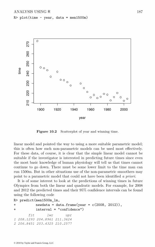
ANALYSIS USING R 187
R> plot(time ~ year, data = men1500m)
1900 1920 1940 1960 1980 2000
21
02
20
23
02
40
25
02
60
27
0
year
tim
e
Figure 10.2 Scatterplot of year and winning time.
linear model and pointed the way to using a more suitable parametric model;this is often how such non-parametric models can be used most effectively.For these data, of course, it is clear that the simple linear model cannot besuitable if the investigator is interested in predicting future times since eventhe most basic knowledge of human physiology will tell us that times cannotcontinue to go down. There must be some lower limit to the time man canrun 1500m. But in other situations use of the non-parametric smoothers maypoint to a parametric model that could not have been identified a priori.
It is of some interest to look at the predictions of winning times in futureOlympics from both the linear and quadratic models. For example, for 2008and 2012 the predicted times and their 95% confidence intervals can be foundusing the following code
R> predict(men1500m_lm,
+ newdata = data.frame(year = c(2008, 2012)),
+ interval = "confidence")
fit lwr upr
1 208.1293 204.8961 211.3624
2 206.8451 203.4325 210.2577
© 2010 by Taylor and Francis Group, LLC

188 SMOOTHERS AND GENERALISED ADDITIVE MODELS
R> men1500m1900 <- subset(men1500m, year >= 1900)
R> men1500m_lm <- lm(time ~ year, data = men1500m1900)
R> plot(time ~ year, data = men1500m1900)
R> abline(men1500m_lm)
1900 1920 1940 1960 1980 2000
21
52
20
22
52
30
23
52
40
24
5
year
tim
e
Figure 10.3 Scatterplot of year and winning time with fitted values from a simple
linear model.
R> predict(men1500m_lm2,
+ newdata = data.frame(year = c(2008, 2012)),
+ interval = "confidence")
fit lwr upr
1 214.2709 210.3930 218.1488
2 214.3314 209.8441 218.8187
For predictions far into the future both the quadratic and the linear model fail;we leave readers to get some more predictions to see what happens. We cancompare the first prediction with the time actually recorded by the winnerof the men’s 1500m in Beijing 2008, Rashid Ramzi from Brunei, who wonthe event in 212.94 seconds. The confidence interval obtained from the simplelinear model does not include this value but the confidence interval for theprediction derived from the quadratic model does.
© 2010 by Taylor and Francis Group, LLC

ANALYSIS USING R 189
R> x <- men1500m1900$year
R> y <- men1500m1900$time
R> men1500m_lowess <- lowess(x, y)
R> plot(time ~ year, data = men1500m1900)
R> lines(men1500m_lowess, lty = 2)
R> men1500m_cubic <- gam(y ~ s(x, bs = "cr"))
R> lines(x, predict(men1500m_cubic), lty = 3)
1900 1920 1940 1960 1980 2000
21
52
20
22
52
30
23
52
40
24
5
year
tim
e
Figure 10.4 Scatterplot of year and winning time with fitted values from a smooth
non-parametric model.
10.3.2 Air Pollution in US Cities
Unfortunately, we cannot fit an additive model for describing the SO2 con-centration based on all six covariates because this leads to more parametersthan cities, i.e., more parameters than observations when using the defaultparameterisation of mgcv. Thus, before we can apply the gam function frompackage mgcv, we have to decide which covariates should enter the model andwhich subset of these covariates should be allowed to deviate from a linearregression relationship.
As briefly discussed in Section 10.2.3, we can fit an additive model using theiterative boosting algorithm as described by Buhlmann and Hothorn (2007).
© 2010 by Taylor and Francis Group, LLC
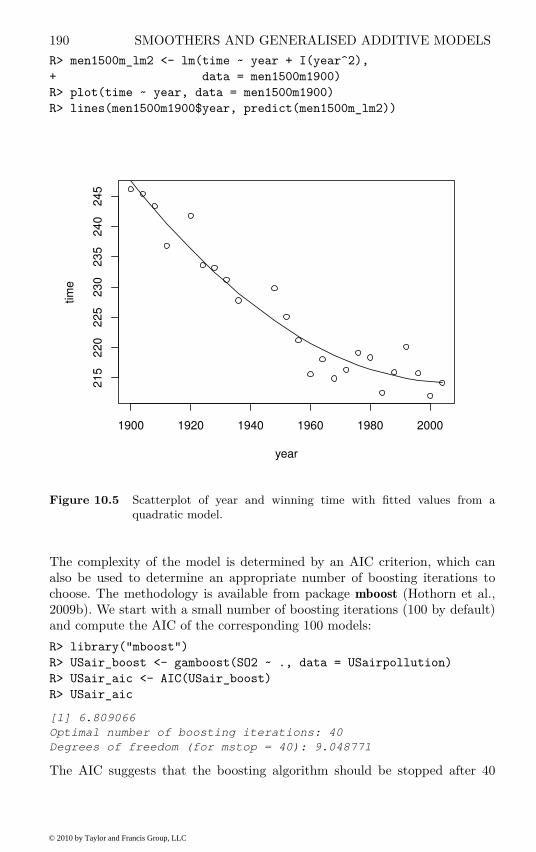
190 SMOOTHERS AND GENERALISED ADDITIVE MODELS
R> men1500m_lm2 <- lm(time ~ year + I(year^2),
+ data = men1500m1900)
R> plot(time ~ year, data = men1500m1900)
R> lines(men1500m1900$year, predict(men1500m_lm2))
1900 1920 1940 1960 1980 2000
21
52
20
22
52
30
23
52
40
24
5
year
tim
e
Figure 10.5 Scatterplot of year and winning time with fitted values from a
quadratic model.
The complexity of the model is determined by an AIC criterion, which canalso be used to determine an appropriate number of boosting iterations tochoose. The methodology is available from package mboost (Hothorn et al.,2009b). We start with a small number of boosting iterations (100 by default)and compute the AIC of the corresponding 100 models:
R> library("mboost")
R> USair_boost <- gamboost(SO2 ~ ., data = USairpollution)
R> USair_aic <- AIC(USair_boost)
R> USair_aic
[1] 6.809066
Optimal number of boosting iterations: 40
Degrees of freedom (for mstop = 40): 9.048771
The AIC suggests that the boosting algorithm should be stopped after 40
© 2010 by Taylor and Francis Group, LLC
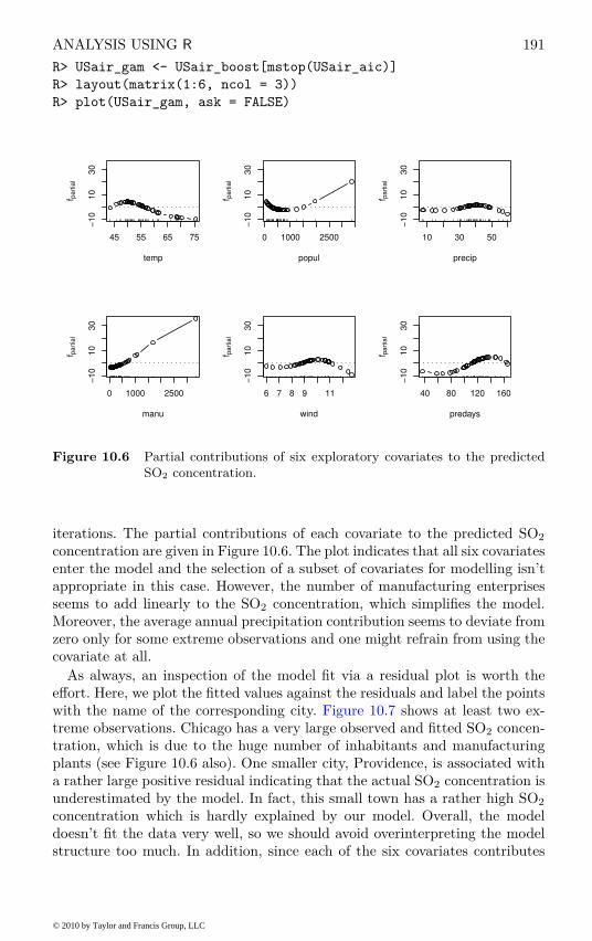
ANALYSIS USING R 191
R> USair_gam <- USair_boost[mstop(USair_aic)]
R> layout(matrix(1:6, ncol = 3))
R> plot(USair_gam, ask = FALSE)
45 55 65 75
−1
01
03
0
temp
f pa
rtia
l
0 1000 2500
−1
01
03
0
manu
f pa
rtia
l
0 1000 2500−
10
10
30
popul
f pa
rtia
l
6 7 8 9 11
−1
01
03
0
wind
f pa
rtia
l
10 30 50
−1
01
03
0
precip
f pa
rtia
l
40 80 120 160−
10
10
30
predays
f pa
rtia
l
Figure 10.6 Partial contributions of six exploratory covariates to the predicted
SO2 concentration.
iterations. The partial contributions of each covariate to the predicted SO2
concentration are given in Figure 10.6. The plot indicates that all six covariatesenter the model and the selection of a subset of covariates for modelling isn’tappropriate in this case. However, the number of manufacturing enterprisesseems to add linearly to the SO2 concentration, which simplifies the model.Moreover, the average annual precipitation contribution seems to deviate fromzero only for some extreme observations and one might refrain from using thecovariate at all.
As always, an inspection of the model fit via a residual plot is worth theeffort. Here, we plot the fitted values against the residuals and label the pointswith the name of the corresponding city. Figure 10.7 shows at least two ex-treme observations. Chicago has a very large observed and fitted SO2 concen-tration, which is due to the huge number of inhabitants and manufacturingplants (see Figure 10.6 also). One smaller city, Providence, is associated witha rather large positive residual indicating that the actual SO2 concentration isunderestimated by the model. In fact, this small town has a rather high SO2
concentration which is hardly explained by our model. Overall, the modeldoesn’t fit the data very well, so we should avoid overinterpreting the modelstructure too much. In addition, since each of the six covariates contributes
© 2010 by Taylor and Francis Group, LLC
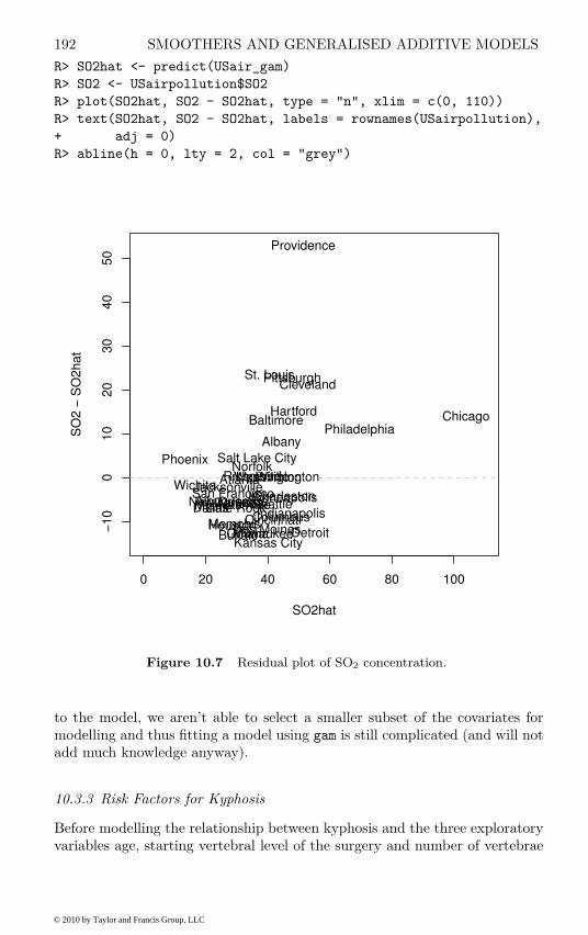
192 SMOOTHERS AND GENERALISED ADDITIVE MODELS
R> SO2hat <- predict(USair_gam)
R> SO2 <- USairpollution$SO2
R> plot(SO2hat, SO2 - SO2hat, type = "n", xlim = c(0, 110))
R> text(SO2hat, SO2 - SO2hat, labels = rownames(USairpollution),
+ adj = 0)
R> abline(h = 0, lty = 2, col = "grey")
0 20 40 60 80 100
−1
00
10
20
30
40
50
SO2hat
SO
2 −
SO
2h
at
Albany
Albuquerque
Atlanta
Baltimore
Buffalo
Charleston
Chicago
Cincinnati
Cleveland
ColumbusDallasDenver
Des MoinesDetroit
Hartford
HoustonIndianapolis
Jacksonville
Kansas City
Little Rock
Louisville
Memphis
Miami
Milwaukee
MinneapolisNashvilleNew Orleans
Norfolk
Omaha
Philadelphia
Phoenix
Pittsburgh
Providence
Richmond
Salt Lake City
San FranciscoSeattle
St. Louis
WashingtonWichita
Wilmington
Figure 10.7 Residual plot of SO2 concentration.
to the model, we aren’t able to select a smaller subset of the covariates formodelling and thus fitting a model using gam is still complicated (and will notadd much knowledge anyway).
10.3.3 Risk Factors for Kyphosis
Before modelling the relationship between kyphosis and the three exploratoryvariables age, starting vertebral level of the surgery and number of vertebrae
© 2010 by Taylor and Francis Group, LLC
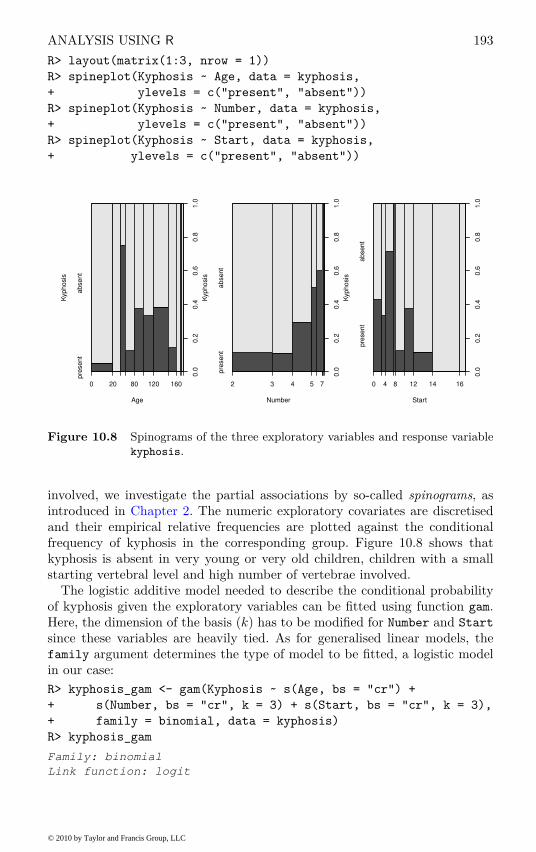
ANALYSIS USING R 193
R> layout(matrix(1:3, nrow = 1))
R> spineplot(Kyphosis ~ Age, data = kyphosis,
+ ylevels = c("present", "absent"))
R> spineplot(Kyphosis ~ Number, data = kyphosis,
+ ylevels = c("present", "absent"))
R> spineplot(Kyphosis ~ Start, data = kyphosis,
+ ylevels = c("present", "absent"))
Age
Kyphosis
0 20 80 120 160
pre
sent
absent
0.0
0.2
0.4
0.6
0.8
1.0
Number
Kyphosis
2 3 4 5 7
pre
sent
absent
0.0
0.2
0.4
0.6
0.8
1.0
Start
Kyphosis
0 4 8 12 14 16
pre
sent
absent
0.0
0.2
0.4
0.6
0.8
1.0
Figure 10.8 Spinograms of the three exploratory variables and response variable
kyphosis.
involved, we investigate the partial associations by so-called spinograms, asintroduced in Chapter 2. The numeric exploratory covariates are discretisedand their empirical relative frequencies are plotted against the conditionalfrequency of kyphosis in the corresponding group. Figure 10.8 shows thatkyphosis is absent in very young or very old children, children with a smallstarting vertebral level and high number of vertebrae involved.
The logistic additive model needed to describe the conditional probabilityof kyphosis given the exploratory variables can be fitted using function gam.Here, the dimension of the basis (k) has to be modified for Number and Start
since these variables are heavily tied. As for generalised linear models, thefamily argument determines the type of model to be fitted, a logistic modelin our case:
R> kyphosis_gam <- gam(Kyphosis ~ s(Age, bs = "cr") +
+ s(Number, bs = "cr", k = 3) + s(Start, bs = "cr", k = 3),
+ family = binomial, data = kyphosis)
R> kyphosis_gam
Family: binomial
Link function: logit
© 2010 by Taylor and Francis Group, LLC
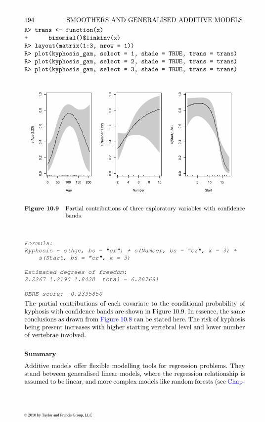
194 SMOOTHERS AND GENERALISED ADDITIVE MODELS
R> trans <- function(x)
+ binomial()$linkinv(x)
R> layout(matrix(1:3, nrow = 1))
R> plot(kyphosis_gam, select = 1, shade = TRUE, trans = trans)
R> plot(kyphosis_gam, select = 2, shade = TRUE, trans = trans)
R> plot(kyphosis_gam, select = 3, shade = TRUE, trans = trans)
0 50 100 150 200
0.0
0.2
0.4
0.6
0.8
1.0
Age
s(A
ge,2
.23)
2 4 6 8 10
0.0
0.2
0.4
0.6
0.8
1.0
Number
s(N
um
ber,
1.2
2)
5 10 150.0
0.2
0.4
0.6
0.8
1.0
Start
s(S
tart
,1.8
4)
Figure 10.9 Partial contributions of three exploratory variables with confidence
bands.
Formula:
Kyphosis ~ s(Age, bs = "cr") + s(Number, bs = "cr", k = 3) +
s(Start, bs = "cr", k = 3)
Estimated degrees of freedom:
2.2267 1.2190 1.8420 total = 6.287681
UBRE score: -0.2335850
The partial contributions of each covariate to the conditional probability ofkyphosis with confidence bands are shown in Figure 10.9. In essence, the sameconclusions as drawn from Figure 10.8 can be stated here. The risk of kyphosisbeing present increases with higher starting vertebral level and lower numberof vertebrae involved.
Summary
Additive models offer flexible modelling tools for regression problems. Theystand between generalised linear models, where the regression relationship isassumed to be linear, and more complex models like random forests (see Chap-
© 2010 by Taylor and Francis Group, LLC

ANALYSIS USING R 195
ter 9) where the regression relationship remains unspecified. Smooth functionsdescribing the influence of covariates on the response can be easily interpreted.Variable selection is a technically difficult problem in this class of models;boosting methods are one possibility to deal with this problem.
Exercises
Ex. 10.1 Consider the body fat data introduced in Chapter 9, Table 9.1.First fit a generalised additive model assuming normal errors using functiongam. Are all potential covariates informative? Check the results against ageneralised additive model that underwent AIC-based variable selection(fitted using function gamboost).
Ex. 10.2 Try to fit a logistic additive model to the glaucoma data discussedin Chapter 9. Which covariates should enter the model and how is theirinfluence on the probability of suffering from glaucoma?
© 2010 by Taylor and Francis Group, LLC

CHAPTER 11
Survival Analysis:Glioma Treatment andBreast Cancer Survival
11.1 Introduction
Grana et al. (2002) report results of a non-randomised clinical trial investi-gating a novel radioimmunotherapy in malignant glioma patients. The overallsurvival, i.e., the time from the beginning of the therapy to the disease-causeddeath of the patient, is compared for two groups of patients. A control groupunderwent the standard therapy and another group of patients was treatedwith radioimmunotherapy in addition. The data, extracted from Tables 1 and2 in Grana et al. (2002), are given in Table 11.1. The main interest is to inves-tigate whether the patients treated with the novel radioimmunotherapy have,on average, longer survival times than patients in the control group.
Table 11.1: glioma data. Patients suffering from two types ofglioma treated with the standard therapy or a novelradioimmunotherapy (RIT).
age sex histology group event time
41 Female Grade3 RIT TRUE 5345 Female Grade3 RIT FALSE 2848 Male Grade3 RIT FALSE 6954 Male Grade3 RIT FALSE 5840 Female Grade3 RIT FALSE 5431 Male Grade3 RIT TRUE 2553 Male Grade3 RIT FALSE 5149 Male Grade3 RIT FALSE 6136 Male Grade3 RIT FALSE 5752 Male Grade3 RIT FALSE 5757 Male Grade3 RIT FALSE 5055 Female GBM RIT FALSE 4370 Male GBM RIT TRUE 2039 Female GBM RIT TRUE 1440 Female GBM RIT FALSE 3647 Female GBM RIT FALSE 5958 Male GBM RIT TRUE 31
197
© 2010 by Taylor and Francis Group, LLC
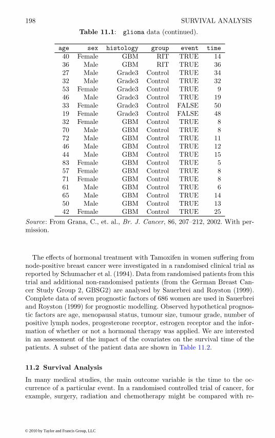
198 SURVIVAL ANALYSIS
Table 11.1: glioma data (continued).
age sex histology group event time
40 Female GBM RIT TRUE 1436 Male GBM RIT TRUE 3627 Male Grade3 Control TRUE 3432 Male Grade3 Control TRUE 3253 Female Grade3 Control TRUE 946 Male Grade3 Control TRUE 1933 Female Grade3 Control FALSE 5019 Female Grade3 Control FALSE 4832 Female GBM Control TRUE 870 Male GBM Control TRUE 872 Male GBM Control TRUE 1146 Male GBM Control TRUE 1244 Male GBM Control TRUE 1583 Female GBM Control TRUE 557 Female GBM Control TRUE 871 Female GBM Control TRUE 861 Male GBM Control TRUE 665 Male GBM Control TRUE 1450 Male GBM Control TRUE 1342 Female GBM Control TRUE 25
Source: From Grana, C., et. al., Br. J. Cancer, 86, 207–212, 2002. With per-mission.
The effects of hormonal treatment with Tamoxifen in women suffering fromnode-positive breast cancer were investigated in a randomised clinical trial asreported by Schumacher et al. (1994). Data from randomised patients from thistrial and additional non-randomised patients (from the German Breast Can-cer Study Group 2, GBSG2) are analysed by Sauerbrei and Royston (1999).Complete data of seven prognostic factors of 686 women are used in Sauerbreiand Royston (1999) for prognostic modelling. Observed hypothetical prognos-tic factors are age, menopausal status, tumour size, tumour grade, number ofpositive lymph nodes, progesterone receptor, estrogen receptor and the infor-mation of whether or not a hormonal therapy was applied. We are interestedin an assessment of the impact of the covariates on the survival time of thepatients. A subset of the patient data are shown in Table 11.2.
11.2 Survival Analysis
In many medical studies, the main outcome variable is the time to the oc-currence of a particular event. In a randomised controlled trial of cancer, forexample, surgery, radiation and chemotherapy might be compared with re-
© 2010 by Taylor and Francis Group, LLC
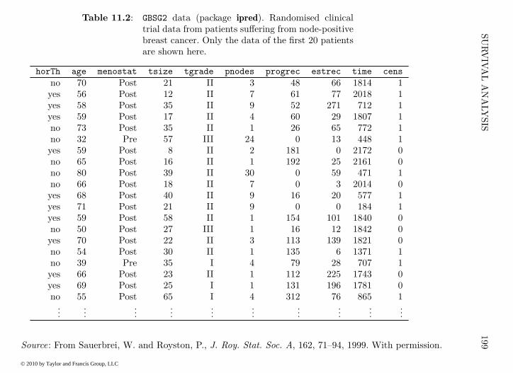
SU
RV
IVA
LA
NA
LY
SIS
199
Table 11.2: GBSG2 data (package ipred). Randomised clinicaltrial data from patients suffering from node-positivebreast cancer. Only the data of the first 20 patientsare shown here.
horTh age menostat tsize tgrade pnodes progrec estrec time cens
no 70 Post 21 II 3 48 66 1814 1yes 56 Post 12 II 7 61 77 2018 1yes 58 Post 35 II 9 52 271 712 1yes 59 Post 17 II 4 60 29 1807 1no 73 Post 35 II 1 26 65 772 1no 32 Pre 57 III 24 0 13 448 1
yes 59 Post 8 II 2 181 0 2172 0no 65 Post 16 II 1 192 25 2161 0no 80 Post 39 II 30 0 59 471 1no 66 Post 18 II 7 0 3 2014 0
yes 68 Post 40 II 9 16 20 577 1yes 71 Post 21 II 9 0 0 184 1yes 59 Post 58 II 1 154 101 1840 0no 50 Post 27 III 1 16 12 1842 0
yes 70 Post 22 II 3 113 139 1821 0no 54 Post 30 II 1 135 6 1371 1no 39 Pre 35 I 4 79 28 707 1
yes 66 Post 23 II 1 112 225 1743 0yes 69 Post 25 I 1 131 196 1781 0no 55 Post 65 I 4 312 76 865 1
......
......
......
......
......
Source: From Sauerbrei, W. and Royston, P., J. Roy. Stat. Soc. A, 162, 71–94, 1999. With permission.
© 2010 by Taylor and Francis Group, LLC

200 SURVIVAL ANALYSIS
spect to time from randomisation and the start of therapy until death. In thiscase, the event of interest is the death of a patient, but in other situations,it might be remission from a disease, relief from symptoms or the recurrenceof a particular condition. Other censored response variables are the time tocredit failure in financial applications or the time a roboter needs to success-fully perform a certain task in engineering. Such observations are generallyreferred to by the generic term survival data even when the endpoint or eventbeing considered is not death but something else. Such data generally requirespecial techniques for analysis for two main reasons:
1. Survival data are generally not symmetrically distributed – they will oftenappear positively skewed, with a few people surviving a very long timecompared with the majority; so assuming a normal distribution will not bereasonable.
2. At the completion of the study, some patients may not have reached theendpoint of interest (death, relapse, etc.). Consequently, the exact survivaltimes are not known. All that is known is that the survival times are greaterthan the amount of time the individual has been in the study. The survivaltimes of these individuals are said to be censored (precisely, they are right-censored).
Of central importance in the analysis of survival time data are two functionsused to describe their distribution, namely the survival (or survivor) function
and the hazard function.
11.2.1 The Survivor Function
The survivor function, S(t), is defined as the probability that the survivaltime, T , is greater than or equal to some time t, i.e.,
S(t) = P(T ≥ t).
A plot of an estimate S(t) of S(t) against the time t is often a useful way ofdescribing the survival experience of a group of individuals. When there areno censored observations in the sample of survival times, a non-parametricsurvivor function can be estimated simply as
S(t) =number of individuals with survival times ≥ t
n
where n is the total number of observations. Because this is simply a propor-tion, confidence intervals can be obtained for each time t by using the varianceestimate
S(t)(1 − S(t))/n.
The simple method used to estimate the survivor function when there areno censored observations cannot now be used for survival times when censoredobservations are present. In the presence of censoring, the survivor functionis typically estimated using the Kaplan-Meier estimator (Kaplan and Meier,
© 2010 by Taylor and Francis Group, LLC

SURVIVAL ANALYSIS 201
1958). This involves first ordering the survival times from the smallest to thelargest such that t(1) ≤ t(2) ≤ · · · ≤ t(n), where t(j) is the jth largest uniquesurvival time. The Kaplan-Meier estimate of the survival function is obtainedas
S(t) =∏
j:t(j)≤t
(
1 −
dj
rj
)
where rj is the number of individuals at risk just before t(j) (including thosecensored at t(j)), and dj is the number of individuals who experience the eventof interest (death, etc.) at time t(j). So, for example, the survivor function atthe second death time, t(2), is equal to the estimated probability of not dyingat time t(2), conditional on the individual being still at risk at time t(2). Theestimated variance of the Kaplan-Meier estimate of the survivor function isfound from
Var(S(t)) =(
S(t))2 ∑
j:t(j)≤t
dj
rj(rj − dj).
A formal test of the equality of the survival curves for the two groups can bemade using the log-rank test. First, the expected number of deaths is computedfor each unique death time, or failure time in the data set, assuming thatthe chances of dying, given that subjects are at risk, are the same for bothgroups. The total number of expected deaths is then computed for each groupby adding the expected number of deaths for each failure time. The test thencompares the observed number of deaths in each group with the expectednumber of deaths using a chi-squared test. Full details and formulae are givenin Therneau and Grambsch (2000) or Everitt and Rabe-Hesketh (2001), forexample.
11.2.2 The Hazard Function
In the analysis of survival data it is often of interest to assess which periodshave high or low chances of death (or whatever the event of interest may be),among those still active at the time. A suitable approach to characterise suchrisks is the hazard function, h(t), defined as the probability that an individualexperiences the event in a small time interval, s, given that the individual hassurvived up to the beginning of the interval, when the size of the time intervalapproaches zero; mathematically this is written as
h(t) = lims→0
P(t ≤ T ≤ t + s|T ≥ t)
s
where T is the individual’s survival time. The conditioning feature of thisdefinition is very important. For example, the probability of dying at age100 is very small because most people die before that age; in contrast, theprobability of a person dying at age 100 who has reached that age is muchgreater.
© 2010 by Taylor and Francis Group, LLC
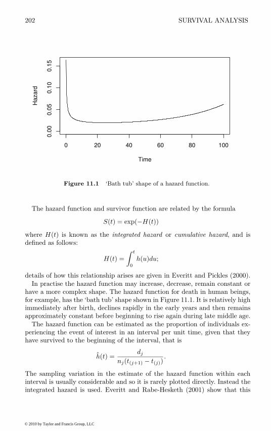
202 SURVIVAL ANALYSIS
0 20 40 60 80 100
0.0
00
.05
0.1
00
.15
Time
Ha
za
rd
Figure 11.1 ‘Bath tub’ shape of a hazard function.
The hazard function and survivor function are related by the formula
S(t) = exp(−H(t))
where H(t) is known as the integrated hazard or cumulative hazard, and isdefined as follows:
H(t) =
∫ t
0
h(u)du;
details of how this relationship arises are given in Everitt and Pickles (2000).In practise the hazard function may increase, decrease, remain constant or
have a more complex shape. The hazard function for death in human beings,for example, has the ‘bath tub’ shape shown in Figure 11.1. It is relatively highimmediately after birth, declines rapidly in the early years and then remainsapproximately constant before beginning to rise again during late middle age.
The hazard function can be estimated as the proportion of individuals ex-periencing the event of interest in an interval per unit time, given that theyhave survived to the beginning of the interval, that is
h(t) =dj
nj(t(j+1) − t(j)).
The sampling variation in the estimate of the hazard function within eachinterval is usually considerable and so it is rarely plotted directly. Instead theintegrated hazard is used. Everitt and Rabe-Hesketh (2001) show that this
© 2010 by Taylor and Francis Group, LLC
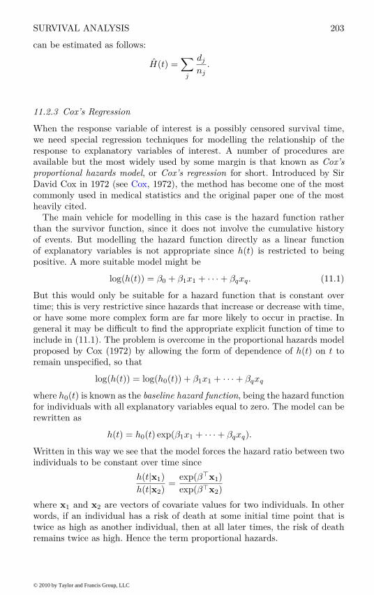
SURVIVAL ANALYSIS 203
can be estimated as follows:
H(t) =∑
j
dj
nj
.
11.2.3 Cox’s Regression
When the response variable of interest is a possibly censored survival time,we need special regression techniques for modelling the relationship of theresponse to explanatory variables of interest. A number of procedures areavailable but the most widely used by some margin is that known as Cox’s
proportional hazards model, or Cox’s regression for short. Introduced by SirDavid Cox in 1972 (see Cox, 1972), the method has become one of the mostcommonly used in medical statistics and the original paper one of the mostheavily cited.
The main vehicle for modelling in this case is the hazard function ratherthan the survivor function, since it does not involve the cumulative historyof events. But modelling the hazard function directly as a linear functionof explanatory variables is not appropriate since h(t) is restricted to beingpositive. A more suitable model might be
log(h(t)) = β0 + β1x1 + · · · + βqxq. (11.1)
But this would only be suitable for a hazard function that is constant overtime; this is very restrictive since hazards that increase or decrease with time,or have some more complex form are far more likely to occur in practise. Ingeneral it may be difficult to find the appropriate explicit function of time toinclude in (11.1). The problem is overcome in the proportional hazards modelproposed by Cox (1972) by allowing the form of dependence of h(t) on t toremain unspecified, so that
log(h(t)) = log(h0(t)) + β1x1 + · · · + βqxq
where h0(t) is known as the baseline hazard function, being the hazard functionfor individuals with all explanatory variables equal to zero. The model can berewritten as
h(t) = h0(t) exp(β1x1 + · · · + βqxq).
Written in this way we see that the model forces the hazard ratio between twoindividuals to be constant over time since
h(t|x1)
h(t|x2)=
exp(β⊤x1)
exp(β⊤x2)
where x1 and x2 are vectors of covariate values for two individuals. In otherwords, if an individual has a risk of death at some initial time point that istwice as high as another individual, then at all later times, the risk of deathremains twice as high. Hence the term proportional hazards.
© 2010 by Taylor and Francis Group, LLC

204 SURVIVAL ANALYSIS
In the Cox model, the baseline hazard describes the common shape of thesurvival time distribution for all individuals, while the relative risk function,exp(β⊤x), gives the level of each individual’s hazard. The interpretation of theparameter βj is that exp(βj) gives the relative risk change associated with anincrease of one unit in covariate xj , all other explanatory variables remainingconstant.
The parameters in a Cox model can be estimated by maximising whatis known as a partial likelihood. Details are given in Kalbfleisch and Pren-tice (1980). The partial likelihood is derived by assuming continuous survivaltimes. In reality, however, survival times are measured in discrete units andthere are often ties. There are three common methods for dealing with tieswhich are described briefly in Everitt and Rabe-Hesketh (2001).
11.3 Analysis Using R
11.3.1 Glioma Radioimmunotherapy
The survival times for patients from the control group and the group treatedwith the novel therapy can be compared graphically by plotting the Kaplan-Meier estimates of the survival times. Here, we plot the Kaplan-Meier esti-mates stratified for patients suffering from grade III glioma and glioblastoma(GBM, grade IV) separately; the results are given in Figure 11.2. The Kaplan-Meier estimates are computed by the survfit function from package survival
(Therneau and Lumley, 2009) which takes a model formula of the form
Surv(time, event) ~ group
where time are the survival times, event is a logical variable being TRUE whenthe event of interest, death for example, has been observed and FALSE whenin case of censoring. The right hand side variable group is a grouping factor.
Figure 11.2 leads to the impression that patients treated with the novelradioimmunotherapy survive longer, regardless of the tumour type. In orderto assess if this informal finding is reliable, we may perform a log-rank testvia
R> survdiff(Surv(time, event) ~ group, data = g3)
Call:
survdiff(formula = Surv(time, event) ~ group, data = g3)
N Observed Expected (O-E)^2/E (O-E)^2/V
group=Control 6 4 1.49 4.23 6.06
group=RIT 11 2 4.51 1.40 6.06
Chisq= 6.1 on 1 degrees of freedom, p= 0.0138
which indicates that the survival times are indeed different in both groups.However, the number of patients is rather limited and so it might be danger-ous to rely on asymptotic tests. As shown in Chapter 4, conditioning on thedata and computing the distribution of the test statistics without additional
© 2010 by Taylor and Francis Group, LLC
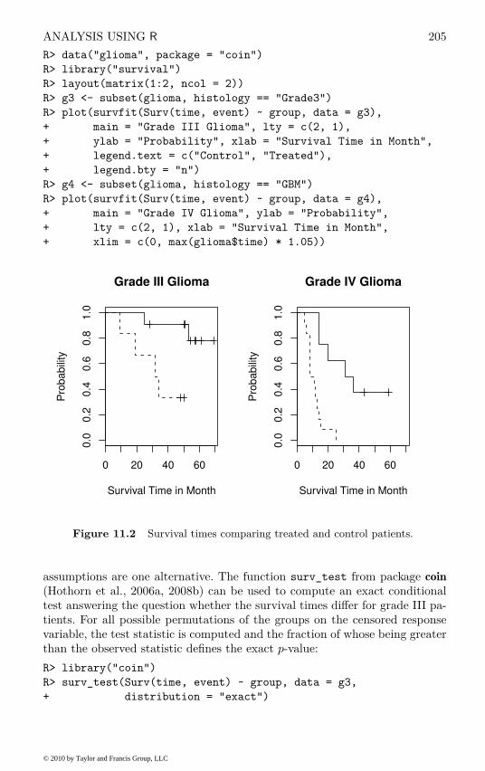
ANALYSIS USING R 205
R> data("glioma", package = "coin")
R> library("survival")
R> layout(matrix(1:2, ncol = 2))
R> g3 <- subset(glioma, histology == "Grade3")
R> plot(survfit(Surv(time, event) ~ group, data = g3),
+ main = "Grade III Glioma", lty = c(2, 1),
+ ylab = "Probability", xlab = "Survival Time in Month",
+ legend.text = c("Control", "Treated"),
+ legend.bty = "n")
R> g4 <- subset(glioma, histology == "GBM")
R> plot(survfit(Surv(time, event) ~ group, data = g4),
+ main = "Grade IV Glioma", ylab = "Probability",
+ lty = c(2, 1), xlab = "Survival Time in Month",
+ xlim = c(0, max(glioma$time) * 1.05))
0 20 40 60
0.0
0.2
0.4
0.6
0.8
1.0
Grade III Glioma
Survival Time in Month
Pro
ba
bili
ty
0 20 40 60
0.0
0.2
0.4
0.6
0.8
1.0
Grade IV Glioma
Survival Time in Month
Pro
ba
bili
ty
Figure 11.2 Survival times comparing treated and control patients.
assumptions are one alternative. The function surv_test from package coin
(Hothorn et al., 2006a, 2008b) can be used to compute an exact conditionaltest answering the question whether the survival times differ for grade III pa-tients. For all possible permutations of the groups on the censored responsevariable, the test statistic is computed and the fraction of whose being greaterthan the observed statistic defines the exact p-value:
R> library("coin")
R> surv_test(Surv(time, event) ~ group, data = g3,
+ distribution = "exact")
© 2010 by Taylor and Francis Group, LLC

206 SURVIVAL ANALYSIS
Exact Logrank Test
data: Surv(time, event) by group (Control, RIT)
Z = 2.1711, p-value = 0.02877
alternative hypothesis: two.sided
which, in this case, confirms the above results. The same exercise can beperformed for patients with grade IV glioma
R> surv_test(Surv(time, event) ~ group, data = g4,
+ distribution = "exact")
Exact Logrank Test
data: Surv(time, event) by group (Control, RIT)
Z = 3.2215, p-value = 0.0001588
alternative hypothesis: two.sided
which shows a difference as well. However, it might be more appropriate toanswer the question whether the novel therapy is superior for both groups oftumours simultaneously. This can be implemented by stratifying, or blocking,with respect to tumour grading:
R> surv_test(Surv(time, event) ~ group | histology,
+ data = glioma, distribution = approximate(B = 10000))
Approximative Logrank Test
data: Surv(time, event) by
group (Control, RIT)
stratified by histology
Z = 3.6704, p-value = 1e-04
alternative hypothesis: two.sided
Here, we need to approximate the exact conditional distribution since the exactdistribution is hard to compute. The result supports the initial impressionimplied by Figure 11.2.
11.3.2 Breast Cancer Survival
Before fitting a Cox model to the GBSG2 data, we again derive a Kaplan-Meierestimate of the survival function of the data, here stratified with respect towhether a patient received a hormonal therapy or not (see Figure 11.3).
Fitting a Cox model follows roughly the same rules as shown for linearmodels in Chapter 6 with the exception that the response variable is againcoded as a Surv object. For the GBSG2 data, the model is fitted via
R> GBSG2_coxph <- coxph(Surv(time, cens) ~ ., data = GBSG2)
and the results as given by the summary method are given in Figure 11.4. Sincewe are especially interested in the relative risk for patients who underwent ahormonal therapy, we can compute an estimate of the relative risk and acorresponding confidence interval via
© 2010 by Taylor and Francis Group, LLC
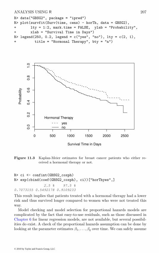
ANALYSIS USING R 207
R> data("GBSG2", package = "ipred")
R> plot(survfit(Surv(time, cens) ~ horTh, data = GBSG2),
+ lty = 1:2, mark.time = FALSE, ylab = "Probability",
+ xlab = "Survival Time in Days")
R> legend(250, 0.2, legend = c("yes", "no"), lty = c(2, 1),
+ title = "Hormonal Therapy", bty = "n")
0 500 1000 1500 2000 2500
0.0
0.2
0.4
0.6
0.8
1.0
Survival Time in Days
Pro
ba
bili
ty
Hormonal Therapy
yesno
Figure 11.3 Kaplan-Meier estimates for breast cancer patients who either re-
ceived a hormonal therapy or not.
R> ci <- confint(GBSG2_coxph)
R> exp(cbind(coef(GBSG2_coxph), ci))["horThyes",]
2.5 % 97.5 %
0.7073155 0.5492178 0.9109233
This result implies that patients treated with a hormonal therapy had a lowerrisk and thus survived longer compared to women who were not treated thisway.
Model checking and model selection for proportional hazards models arecomplicated by the fact that easy-to-use residuals, such as those discussed inChapter 6 for linear regression models, are not available, but several possibil-ities do exist. A check of the proportional hazards assumption can be done bylooking at the parameter estimates β1, . . . , βq over time. We can safely assume
© 2010 by Taylor and Francis Group, LLC

208 SURVIVAL ANALYSIS
R> summary(GBSG2_coxph)
Call:
coxph(formula = Surv(time, cens) ~ ., data = GBSG2)
n= 686
coef exp(coef) se(coef) z Pr(>|z|)
horThyes -0.3462784 0.7073155 0.1290747 -2.683 0.007301
age -0.0094592 0.9905854 0.0093006 -1.017 0.309126
menostatPost 0.2584448 1.2949147 0.1834765 1.409 0.158954
tsize 0.0077961 1.0078266 0.0039390 1.979 0.047794
tgrade.L 0.5512988 1.7355056 0.1898441 2.904 0.003685
tgrade.Q -0.2010905 0.8178384 0.1219654 -1.649 0.099199
pnodes 0.0487886 1.0499984 0.0074471 6.551 5.7e-11
progrec -0.0022172 0.9977852 0.0005735 -3.866 0.000111
estrec 0.0001973 1.0001973 0.0004504 0.438 0.661307
exp(coef) exp(-coef) lower .95 upper .95
horThyes 0.7073 1.4138 0.5492 0.911
age 0.9906 1.0095 0.9727 1.009
menostatPost 1.2949 0.7723 0.9038 1.855
tsize 1.0078 0.9922 1.0001 1.016
tgrade.L 1.7355 0.5762 1.1963 2.518
tgrade.Q 0.8178 1.2227 0.6439 1.039
pnodes 1.0500 0.9524 1.0348 1.065
progrec 0.9978 1.0022 0.9967 0.999
estrec 1.0002 0.9998 0.9993 1.001
Rsquare= 0.142 (max possible= 0.995 )
Likelihood ratio test= 104.8 on 9 df, p=0
Wald test = 114.8 on 9 df, p=0
Score (logrank) test = 120.7 on 9 df, p=0
Figure 11.4 R output of the summary method for GBSG2_coxph.
proportional hazards when the estimates don’t vary much over time. The nullhypothesis of constant regression coefficients can be tested, both globally aswell as for each covariate, by using the cox.zph function
R> GBSG2_zph <- cox.zph(GBSG2_coxph)
R> GBSG2_zph
rho chisq p
horThyes -2.54e-02 1.96e-01 0.65778
age 9.40e-02 2.96e+00 0.08552
menostatPost -1.19e-05 3.75e-08 0.99985
tsize -2.50e-02 1.88e-01 0.66436
tgrade.L -1.30e-01 4.85e+00 0.02772
© 2010 by Taylor and Francis Group, LLC
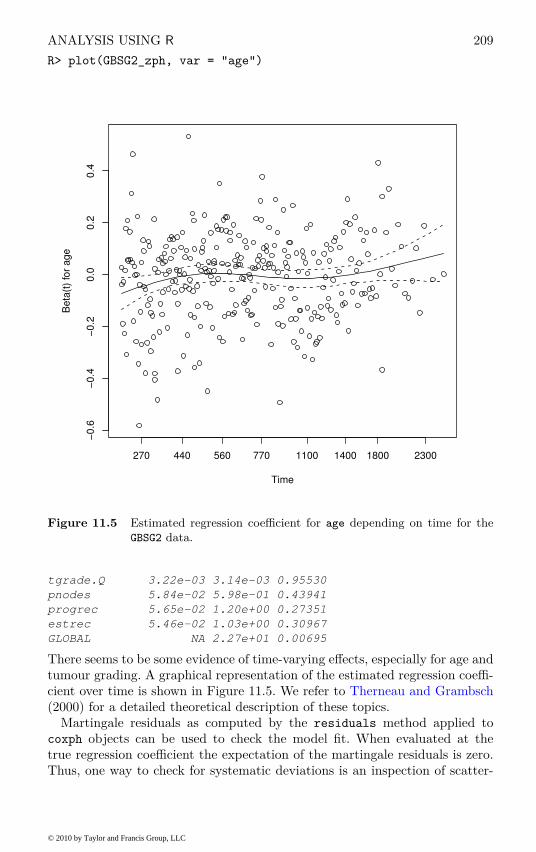
ANALYSIS USING R 209
R> plot(GBSG2_zph, var = "age")
Time
Be
ta(t
) fo
r a
ge
270 440 560 770 1100 1400 1800 2300
−0
.6−
0.4
−0
.20
.00
.20
.4
Figure 11.5 Estimated regression coefficient for age depending on time for the
GBSG2 data.
tgrade.Q 3.22e-03 3.14e-03 0.95530
pnodes 5.84e-02 5.98e-01 0.43941
progrec 5.65e-02 1.20e+00 0.27351
estrec 5.46e-02 1.03e+00 0.30967
GLOBAL NA 2.27e+01 0.00695
There seems to be some evidence of time-varying effects, especially for age andtumour grading. A graphical representation of the estimated regression coeffi-cient over time is shown in Figure 11.5. We refer to Therneau and Grambsch(2000) for a detailed theoretical description of these topics.
Martingale residuals as computed by the residuals method applied tocoxph objects can be used to check the model fit. When evaluated at thetrue regression coefficient the expectation of the martingale residuals is zero.Thus, one way to check for systematic deviations is an inspection of scatter-
© 2010 by Taylor and Francis Group, LLC

210 SURVIVAL ANALYSIS
R> layout(matrix(1:3, ncol = 3))
R> res <- residuals(GBSG2_coxph)
R> plot(res ~ age, data = GBSG2, ylim = c(-2.5, 1.5),
+ pch = ".", ylab = "Martingale Residuals")
R> abline(h = 0, lty = 3)
R> plot(res ~ pnodes, data = GBSG2, ylim = c(-2.5, 1.5),
+ pch = ".", ylab = "")
R> abline(h = 0, lty = 3)
R> plot(res ~ log(progrec), data = GBSG2, ylim = c(-2.5, 1.5),
+ pch = ".", ylab = "")
R> abline(h = 0, lty = 3)
20 40 60 80
−2
−1
01
age
Ma
rtin
ga
le R
esid
ua
ls
0 10 20 30 40 50
−2
−1
01
pnodes
0 2 4 6 8
−2
−1
01
log(progrec)
Figure 11.6 Martingale residuals for the GBSG2 data.
plots plotting covariates against the martingale residuals. For the GBSG2 data,Figure 11.6 does not indicate severe and systematic deviations from zero.
The tree-structured regression models applied to continuous and binaryresponses in Chapter 9 are applicable to censored responses in survival analysisas well. Such a simple prognostic model with only a few terminal nodes mightbe helpful for relating the risk to certain subgroups of patients. Both rpart
and the ctree function from package party can be applied to the GBSG2data, where the conditional trees of the latter select cutpoints based on log-rank statistics
R> GBSG2_ctree <- ctree(Surv(time, cens) ~ ., data = GBSG2)
and the plot method applied to this tree produces the graphical representationin Figure 11.7. The number of positive lymph nodes (pnodes) is the most
© 2010 by Taylor and Francis Group, LLC
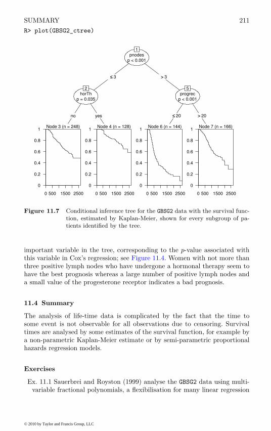
SUMMARY 211
R> plot(GBSG2_ctree)
pnodesp < 0.001
1
≤≤ 3 >> 3
horThp = 0.035
2
no yes
Node 3 (n = 248)
0 500 1500 2500
0
0.2
0.4
0.6
0.8
1Node 4 (n = 128)
0 500 1500 2500
0
0.2
0.4
0.6
0.8
1
progrecp < 0.001
5
≤≤ 20 >> 20
Node 6 (n = 144)
0 500 1500 2500
0
0.2
0.4
0.6
0.8
1Node 7 (n = 166)
0 500 1500 2500
0
0.2
0.4
0.6
0.8
1
Figure 11.7 Conditional inference tree for the GBSG2 data with the survival func-
tion, estimated by Kaplan-Meier, shown for every subgroup of pa-
tients identified by the tree.
important variable in the tree, corresponding to the p-value associated withthis variable in Cox’s regression; see Figure 11.4. Women with not more thanthree positive lymph nodes who have undergone a hormonal therapy seem tohave the best prognosis whereas a large number of positive lymph nodes anda small value of the progesterone receptor indicates a bad prognosis.
11.4 Summary
The analysis of life-time data is complicated by the fact that the time tosome event is not observable for all observations due to censoring. Survivaltimes are analysed by some estimates of the survival function, for example bya non-parametric Kaplan-Meier estimate or by semi-parametric proportionalhazards regression models.
Exercises
Ex. 11.1 Sauerbrei and Royston (1999) analyse the GBSG2 data using multi-variable fractional polynomials, a flexibilisation for many linear regression
© 2010 by Taylor and Francis Group, LLC
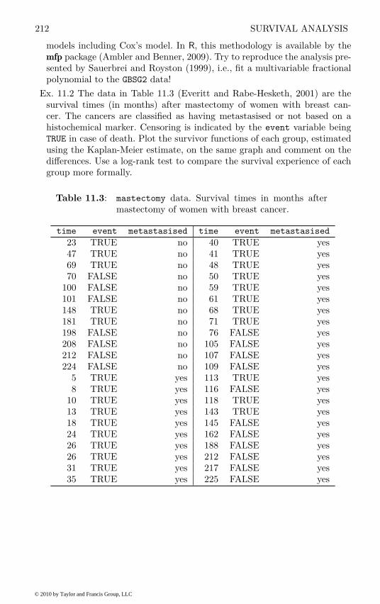
212 SURVIVAL ANALYSIS
models including Cox’s model. In R, this methodology is available by themfp package (Ambler and Benner, 2009). Try to reproduce the analysis pre-sented by Sauerbrei and Royston (1999), i.e., fit a multivariable fractionalpolynomial to the GBSG2 data!
Ex. 11.2 The data in Table 11.3 (Everitt and Rabe-Hesketh, 2001) are thesurvival times (in months) after mastectomy of women with breast can-cer. The cancers are classified as having metastasised or not based on ahistochemical marker. Censoring is indicated by the event variable beingTRUE in case of death. Plot the survivor functions of each group, estimatedusing the Kaplan-Meier estimate, on the same graph and comment on thedifferences. Use a log-rank test to compare the survival experience of eachgroup more formally.
Table 11.3: mastectomy data. Survival times in months aftermastectomy of women with breast cancer.
time event metastasised time event metastasised
23 TRUE no 40 TRUE yes47 TRUE no 41 TRUE yes69 TRUE no 48 TRUE yes70 FALSE no 50 TRUE yes
100 FALSE no 59 TRUE yes101 FALSE no 61 TRUE yes148 TRUE no 68 TRUE yes181 TRUE no 71 TRUE yes198 FALSE no 76 FALSE yes208 FALSE no 105 FALSE yes212 FALSE no 107 FALSE yes224 FALSE no 109 FALSE yes
5 TRUE yes 113 TRUE yes8 TRUE yes 116 FALSE yes
10 TRUE yes 118 TRUE yes13 TRUE yes 143 TRUE yes18 TRUE yes 145 FALSE yes24 TRUE yes 162 FALSE yes26 TRUE yes 188 FALSE yes26 TRUE yes 212 FALSE yes31 TRUE yes 217 FALSE yes35 TRUE yes 225 FALSE yes
© 2010 by Taylor and Francis Group, LLC

CHAPTER 12
Analysing Longitudinal Data I:Computerised Delivery of Cognitive
Behavioural Therapy – Beat the Blues
12.1 Introduction
Depression is a major public health problem across the world. Antidepressantsare the front line treatment, but many patients either do not respond to them,or do not like taking them. The main alternative is psychotherapy, and themodern ‘talking treatments’ such as cognitive behavioural therapy (CBT) havebeen shown to be as effective as drugs, and probably more so when it comesto relapse. But there is a problem, namely availability–there are simply notenough skilled therapists to meet the demand, and little prospect at all of thissituation changing.
A number of alternative modes of delivery of CBT have been explored, in-cluding interactive systems making use of the new computer technologies. Theprinciples of CBT lend themselves reasonably well to computerisation, and,perhaps surprisingly, patients adapt well to this procedure, and do not seemto miss the physical presence of the therapist as much as one might expect.The data to be used in this chapter arise from a clinical trial of an interactive,multimedia program known as ‘Beat the Blues’ designed to deliver cognitivebehavioural therapy to depressed patients via a computer terminal. Full detailsare given in Proudfoot et al. (2003), but in essence Beat the Blues is an in-teractive program using multimedia techniques, in particular video vignettes.The computer-based intervention consists of nine sessions, followed by eighttherapy sessions, each lasting about 50 minutes. Nurses are used to explainhow the program works, but are instructed to spend no more than 5 minuteswith each patient at the start of each session, and are there simply to assistwith the technology. In a randomised controlled trial of the program, patientswith depression recruited in primary care were randomised to either the Beatthe Blues program or to ‘Treatment as Usual’ (TAU). Patients randomisedto Beat the Blues also received pharmacology and/or general practise (GP)support and practical/social help, offered as part of treatment as usual, withthe exception of any face-to-face counselling or psychological intervention.Patients allocated to TAU received whatever treatment their GP prescribed.The latter included, besides any medication, discussion of problems with GP,provision of practical/social help, referral to a counsellor, referral to a prac-
213
© 2010 by Taylor and Francis Group, LLC

214 ANALYSING LONGITUDINAL DATA I
tise nurse, referral to mental health professionals (psychologist, psychiatrist,community psychiatric nurse, counsellor), or further physical examination.
A number of outcome measures were used in the trial, but here we concen-trate on the Beck Depression Inventory II (BDI, Beck et al., 1996). Measure-ments on this variable were made on the following five occasions:
• Prior to treatment,
• Two months after treatment began and
• At one, three and six months follow-up, i.e., at three, five and eight monthsafter treatment.
Table 12.1: BtheB data. Data of a randomised trial evaluatingthe effects of Beat the Blues.
drug length treatment bdi.pre bdi.2m bdi.3m bdi.5m bdi.8m
No >6m TAU 29 2 2 NA NAYes >6m BtheB 32 16 24 17 20Yes <6m TAU 25 20 NA NA NANo >6m BtheB 21 17 16 10 9Yes >6m BtheB 26 23 NA NA NAYes <6m BtheB 7 0 0 0 0Yes <6m TAU 17 7 7 3 7No >6m TAU 20 20 21 19 13Yes <6m BtheB 18 13 14 20 11Yes >6m BtheB 20 5 5 8 12No >6m TAU 30 32 24 12 2Yes <6m BtheB 49 35 NA NA NANo >6m TAU 26 27 23 NA NAYes >6m TAU 30 26 36 27 22Yes >6m BtheB 23 13 13 12 23No <6m TAU 16 13 3 2 0No >6m BtheB 30 30 29 NA NANo <6m BtheB 13 8 8 7 6No >6m TAU 37 30 33 31 22Yes <6m BtheB 35 12 10 8 10No >6m BtheB 21 6 NA NA NANo <6m TAU 26 17 17 20 12No >6m TAU 29 22 10 NA NANo >6m TAU 20 21 NA NA NANo >6m TAU 33 23 NA NA NANo >6m BtheB 19 12 13 NA NAYes <6m TAU 12 15 NA NA NAYes >6m TAU 47 36 49 34 NAYes >6m BtheB 36 6 0 0 2No <6m BtheB 10 8 6 3 3
© 2010 by Taylor and Francis Group, LLC
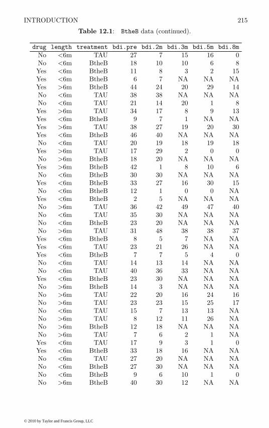
INTRODUCTION 215
Table 12.1: BtheB data (continued).
drug length treatment bdi.pre bdi.2m bdi.3m bdi.5m bdi.8m
No <6m TAU 27 7 15 16 0No <6m BtheB 18 10 10 6 8Yes <6m BtheB 11 8 3 2 15Yes <6m BtheB 6 7 NA NA NAYes >6m BtheB 44 24 20 29 14No <6m TAU 38 38 NA NA NANo <6m TAU 21 14 20 1 8Yes >6m TAU 34 17 8 9 13Yes <6m BtheB 9 7 1 NA NAYes >6m TAU 38 27 19 20 30Yes <6m BtheB 46 40 NA NA NANo <6m TAU 20 19 18 19 18Yes >6m TAU 17 29 2 0 0No >6m BtheB 18 20 NA NA NAYes >6m BtheB 42 1 8 10 6No <6m BtheB 30 30 NA NA NAYes <6m BtheB 33 27 16 30 15No <6m BtheB 12 1 0 0 NAYes <6m BtheB 2 5 NA NA NANo >6m TAU 36 42 49 47 40No <6m TAU 35 30 NA NA NANo <6m BtheB 23 20 NA NA NANo >6m TAU 31 48 38 38 37Yes <6m BtheB 8 5 7 NA NAYes <6m TAU 23 21 26 NA NAYes <6m BtheB 7 7 5 4 0No <6m TAU 14 13 14 NA NANo <6m TAU 40 36 33 NA NAYes <6m BtheB 23 30 NA NA NANo >6m BtheB 14 3 NA NA NANo >6m TAU 22 20 16 24 16No >6m TAU 23 23 15 25 17No <6m TAU 15 7 13 13 NANo >6m TAU 8 12 11 26 NANo >6m BtheB 12 18 NA NA NANo >6m TAU 7 6 2 1 NAYes <6m TAU 17 9 3 1 0Yes <6m BtheB 33 18 16 NA NANo <6m TAU 27 20 NA NA NANo <6m BtheB 27 30 NA NA NANo <6m BtheB 9 6 10 1 0No >6m BtheB 40 30 12 NA NA
© 2010 by Taylor and Francis Group, LLC

216 ANALYSING LONGITUDINAL DATA I
Table 12.1: BtheB data (continued).
drug length treatment bdi.pre bdi.2m bdi.3m bdi.5m bdi.8m
No >6m TAU 11 8 7 NA NANo <6m TAU 9 8 NA NA NANo >6m TAU 14 22 21 24 19Yes >6m BtheB 28 9 20 18 13No >6m BtheB 15 9 13 14 10Yes >6m BtheB 22 10 5 5 12No <6m TAU 23 9 NA NA NANo >6m TAU 21 22 24 23 22No >6m TAU 27 31 28 22 14Yes >6m BtheB 14 15 NA NA NANo >6m TAU 10 13 12 8 20Yes <6m TAU 21 9 6 7 1Yes >6m BtheB 46 36 53 NA NANo >6m BtheB 36 14 7 15 15Yes >6m BtheB 23 17 NA NA NAYes >6m TAU 35 0 6 0 1Yes <6m BtheB 33 13 13 10 8No <6m BtheB 19 4 27 1 2No <6m TAU 16 NA NA NA NAYes <6m BtheB 30 26 28 NA NAYes <6m BtheB 17 8 7 12 NANo >6m BtheB 19 4 3 3 3No >6m BtheB 16 11 4 2 3Yes >6m BtheB 16 16 10 10 8Yes <6m TAU 28 NA NA NA NANo >6m BtheB 11 22 9 11 11No <6m TAU 13 5 5 0 6Yes <6m TAU 43 NA NA NA NA
The resulting data from a subset of 100 patients are shown in Table 12.1.(The data are used with the kind permission of Dr. Judy Proudfoot.) In ad-dition to assessing the effects of treatment, there is interest here in assessingthe effect of taking antidepressant drugs (drug, yes or no) and length of thecurrent episode of depression (length, less or more than six months).
12.2 Analysing Longitudinal Data
The distinguishing feature of a longitudinal study is that the response vari-able of interest and a set of explanatory variables are measured several timeson each individual in the study. The main objective in such a study is tocharacterise change in the repeated values of the response variable and to de-
© 2010 by Taylor and Francis Group, LLC

LINEAR MIXED EFFECTS MODELS 217
termine the explanatory variables most associated with any change. Becauseseveral observations of the response variable are made on the same individual,it is likely that the measurements will be correlated rather than independent,even after conditioning on the explanatory variables. Consequently repeatedmeasures data require special methods of analysis and models for such dataneed to include parameters linking the explanatory variables to the repeatedmeasurements, parameters analogous to those in the usual multiple regressionmodel (see Chapter 6), and, in addition parameters that account for the cor-relational structure of the repeated measurements. It is the former parametersthat are generally of most interest with the latter often being regarded as nui-sance parameters. But providing an adequate description for the correlationalstructure of the repeated measures is necessary to avoid misleading inferencesabout the parameters that are of real interest to the researcher.
Over the last decade methodology for the analysis of repeated measuresdata has been the subject of much research and development, and there arenow a variety of powerful techniques available. A comprehensive account ofthese methods is given in Diggle et al. (2003) and Davis (2002). In this chapterwe will concentrate on a single class of methods, linear mixed effects modelssuitable when, conditional on the explanatory variables, the response has anormal distribution. In Chapter 13 two other classes of models which can dealwith non-normal responses will be described.
12.3 Linear Mixed Effects Models for Repeated Measures Data
Linear mixed effects models for repeated measures data formalise the sensibleidea that an individual’s pattern of responses is likely to depend on manycharacteristics of that individual, including some that are unobserved. Theseunobserved variables are then included in the model as random variables,i.e., random effects. The essential feature of such models is that correlationamongst the repeated measurements on the same unit arises from shared,unobserved variables. Conditional on the values of the random effects, therepeated measurements are assumed to be independent, the so-called localindependence assumption.
Two commonly used linear mixed effect models, the random intercept andthe random intercept and slope models, will now be described in more detail.
Let yij represent the observation made at time tj on individual i. A possiblemodel for the observation yij might be
yij = β0 + β1tj + ui + εij . (12.1)
Here the total residual that would be present in the usual linear regressionmodel has been partitioned into a subject-specific random component ui whichis constant over time plus a residual εij which varies randomly over time.The ui are assumed to be normally distributed with zero mean and varianceσ2
u. Similarly the residuals εij are assumed normally distributed with zeromean and variance σ2. The ui and εij are assumed to be independent of each
© 2010 by Taylor and Francis Group, LLC

218 ANALYSING LONGITUDINAL DATA I
other and of the time tj . The model in (12.1) is known as a random interceptmodel, the ui being the random intercepts. The repeated measurements for anindividual vary about that individual’s own regression line which can differ inintercept but not in slope from the regression lines of other individuals. Therandom effects model possible heterogeneity in the intercepts of the individualswhereas time has a fixed effect, β1.
The random intercept model implies that the total variance of each repeatedmeasurement is Var(yij) = Var(ui + εij) = σ2
u +σ2. Due to this decompositionof the total residual variance into a between-subject component, σ2
u, and awithin-subject component, σ2, the model is sometimes referred to as a variancecomponent model.
The covariance between the total residuals at two time points j and k in thesame individual is Cov(ui +εij , ui +εik) = σ2
u. Note that these covariances areinduced by the shared random intercept; for individuals with ui > 0, the totalresiduals will tend to be greater than the mean, for individuals with ui < 0they will tend to be less than the mean. It follows from the two relations abovethat the residual correlations are given by
Cor(ui + εij , ui + εik) =σ2
u
σ2u + σ2
.
This is an intra-class correlation interpreted as the proportion of the totalresidual variance that is due to residual variability between subjects. A randomintercept model constrains the variance of each repeated measure to be thesame and the covariance between any pair of measurements to be equal. This isusually called the compound symmetry structure. These constraints are oftennot realistic for repeated measures data. For example, for longitudinal data it ismore common for measures taken closer to each other in time to be more highlycorrelated than those taken further apart. In addition the variances of the laterrepeated measures are often greater than those taken earlier. Consequentlyfor many such data sets the random intercept model will not do justice tothe observed pattern of covariances between the repeated measures. A modelthat allows a more realistic structure for the covariances is one that allowsheterogeneity in both slopes and intercepts, the random slope and interceptmodel.
In this model there are two types of random effects, the first modellingheterogeneity in intercepts, ui, and the second modelling heterogeneity inslopes, vi. Explicitly the model is
yij = β0 + β1tj + ui + vitj + εij (12.2)
where the parameters are not, of course, the same as in (12.1). The two randomeffects are assumed to have a bivariate normal distribution with zero meansfor both variables and variances σ2
u and σ2v with covariance σuv. With this
model the total residual is ui + uitj + εij with variance
Var(ui + vitj + εij) = σ2
u + 2σuvtj + σ2
vt2
j + σ2
© 2010 by Taylor and Francis Group, LLC

ANALYSIS USING R 219
which is no longer constant for different values of tj . Similarly the covariancebetween two total residuals of the same individual
Cov(ui + vitj + εij , ui + vitk + εik) = σ2
u + σuv(tj − tk) + σ2
vtjtk
is not constrained to be the same for all pairs tj and tk.(It should also be noted that re-estimating the model after adding or sub-
tracting a constant from tj , e.g., its mean, will lead to different variance andcovariance estimates, but will not affect fixed effects.)
Linear mixed-effects models can be estimated by maximum likelihood. How-ever, this method tends to underestimate the variance components. A modi-fied version of maximum likelihood, known as restricted maximum likelihoodis therefore often recommended; this provides consistent estimates of the vari-ance components. Details are given in Diggle et al. (2003) and Longford (1993).Competing linear mixed-effects models can be compared using a likelihood ra-tio test. If however the models have been estimated by restricted maximumlikelihood this test can be used only if both models have the same set of fixedeffects, see Longford (1993). (It should be noted that there are some tech-nical problems with the likelihood ratio test which are discussed in detail inRabe-Hesketh and Skrondal, 2008).
12.4 Analysis Using R
Almost all statistical analyses should begin with some graphical representationof the data and here we shall construct the boxplots of each of the five repeatedmeasures separately for each treatment group. The data are available as thedata frame BtheB and the necessary R code is given along with Figure 12.1.The boxplots show that there is decline in BDI values in both groups withperhaps the values in the group of patients treated in the Beat the Blues armbeing lower at each post-randomisation visit.
We shall fit both random intercept and random intercept and slope modelsto the data including the baseline BDI values (pre.bdi), treatment group,drug and length as fixed effect covariates. Linear mixed effects models arefitted in R by using the lmer function contained in the lme4 package (Batesand Sarkar, 2008, Pinheiro and Bates, 2000, Bates, 2005), but an essentialfirst step is to rearrange the data from the ‘wide form’ in which they appearin the BtheB data frame into the ‘long form’ in which each separate repeatedmeasurement and associated covariate values appear as a separate row in adata.frame. This rearrangement can be made using the following code:
R> data("BtheB", package = "HSAUR2")
R> BtheB$subject <- factor(rownames(BtheB))
R> nobs <- nrow(BtheB)
R> BtheB_long <- reshape(BtheB, idvar = "subject",
+ varying = c("bdi.2m", "bdi.3m", "bdi.5m", "bdi.8m"),
+ direction = "long")
R> BtheB_long$time <- rep(c(2, 3, 5, 8), rep(nobs, 4))
© 2010 by Taylor and Francis Group, LLC
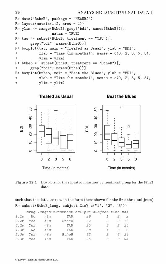
220 ANALYSING LONGITUDINAL DATA I
R> data("BtheB", package = "HSAUR2")
R> layout(matrix(1:2, nrow = 1))
R> ylim <- range(BtheB[,grep("bdi", names(BtheB))],
+ na.rm = TRUE)
R> tau <- subset(BtheB, treatment == "TAU")[,
+ grep("bdi", names(BtheB))]
R> boxplot(tau, main = "Treated as Usual", ylab = "BDI",
+ xlab = "Time (in months)", names = c(0, 2, 3, 5, 8),
+ ylim = ylim)
R> btheb <- subset(BtheB, treatment == "BtheB")[,
+ grep("bdi", names(BtheB))]
R> boxplot(btheb, main = "Beat the Blues", ylab = "BDI",
+ xlab = "Time (in months)", names = c(0, 2, 3, 5, 8),
+ ylim = ylim)
0 2 3 5 8
01
02
03
04
05
0
Treated as Usual
Time (in months)
BD
I
0 2 3 5 8
01
02
03
04
05
0Beat the Blues
Time (in months)
BD
I
Figure 12.1 Boxplots for the repeated measures by treatment group for the BtheB
data.
such that the data are now in the form (here shown for the first three subjects)
R> subset(BtheB_long, subject %in% c("1", "2", "3"))
drug length treatment bdi.pre subject time bdi
1.2m No >6m TAU 29 1 2 2
2.2m Yes >6m BtheB 32 2 2 16
3.2m Yes <6m TAU 25 3 2 20
1.3m No >6m TAU 29 1 3 2
2.3m Yes >6m BtheB 32 2 3 24
3.3m Yes <6m TAU 25 3 3 NA
© 2010 by Taylor and Francis Group, LLC

ANALYSIS USING R 221
1.5m No >6m TAU 29 1 5 NA
2.5m Yes >6m BtheB 32 2 5 17
3.5m Yes <6m TAU 25 3 5 NA
1.8m No >6m TAU 29 1 8 NA
2.8m Yes >6m BtheB 32 2 8 20
3.8m Yes <6m TAU 25 3 8 NA
The resulting data.frame BtheB_long contains a number of missing valuesand in applying the lmer function these will be dropped. But notice it is onlythe missing values that are removed, not participants that have at least onemissing value. All the available data is used in the model fitting process. Thelmer function is used in a similar way to the lm function met in Chapter 6with the addition of a random term to identify the source of the repeatedmeasurements, here subject. We can fit the two models (12.1) and (12.2)and test which is most appropriate using
R> library("lme4")
R> BtheB_lmer1 <- lmer(bdi ~ bdi.pre + time + treatment + drug +
+ length + (1 | subject), data = BtheB_long,
+ REML = FALSE, na.action = na.omit)
R> BtheB_lmer2 <- lmer(bdi ~ bdi.pre + time + treatment + drug +
+ length + (time | subject), data = BtheB_long,
+ REML = FALSE, na.action = na.omit)
R> anova(BtheB_lmer1, BtheB_lmer2)
Data: BtheB_long
Models:
BtheB_lmer1: bdi ~ bdi.pre + time + treatment + drug + length +
BtheB_lmer1: (1 | subject)
BtheB_lmer2: bdi ~ bdi.pre + time + treatment + drug + length +
BtheB_lmer2: (time | subject)
Df AIC BIC logLik Chisq Chi Df
BtheB_lmer1 8 1887.49 1916.57 -935.75
BtheB_lmer2 10 1891.04 1927.39 -935.52 0.4542 2
Pr(>Chisq)
BtheB_lmer1
BtheB_lmer2 0.7969
The log-likelihood test indicates that the simpler random intercept modelis adequate for these data. More information about the fitted random inter-cept model can be extracted from object BtheB_lmer1 using summary by theR code in Figure 12.2. We see that the regression coefficients for time andthe Beck Depression Inventory II values measured at baseline (bdi.pre) arehighly significant, but there is no evidence that the coefficients for the otherthree covariates differ from zero. In particular, there is no clear evidence of atreatment effect.
The summary method for lmer objects doesn’t print p-values for Gaussianmixed models because the degrees of freedom of the t reference distribution arenot obvious. However, one can rely on the asymptotic normal distribution for
© 2010 by Taylor and Francis Group, LLC
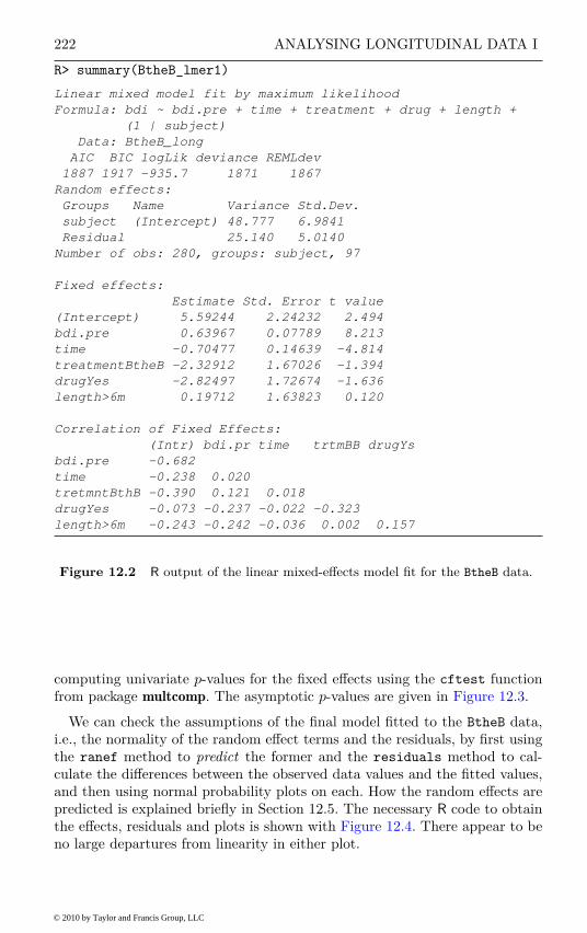
222 ANALYSING LONGITUDINAL DATA I
R> summary(BtheB_lmer1)
Linear mixed model fit by maximum likelihood
Formula: bdi ~ bdi.pre + time + treatment + drug + length +
(1 | subject)
Data: BtheB_long
AIC BIC logLik deviance REMLdev
1887 1917 -935.7 1871 1867
Random effects:
Groups Name Variance Std.Dev.
subject (Intercept) 48.777 6.9841
Residual 25.140 5.0140
Number of obs: 280, groups: subject, 97
Fixed effects:
Estimate Std. Error t value
(Intercept) 5.59244 2.24232 2.494
bdi.pre 0.63967 0.07789 8.213
time -0.70477 0.14639 -4.814
treatmentBtheB -2.32912 1.67026 -1.394
drugYes -2.82497 1.72674 -1.636
length>6m 0.19712 1.63823 0.120
Correlation of Fixed Effects:
(Intr) bdi.pr time trtmBB drugYs
bdi.pre -0.682
time -0.238 0.020
tretmntBthB -0.390 0.121 0.018
drugYes -0.073 -0.237 -0.022 -0.323
length>6m -0.243 -0.242 -0.036 0.002 0.157
Figure 12.2 R output of the linear mixed-effects model fit for the BtheB data.
computing univariate p-values for the fixed effects using the cftest functionfrom package multcomp. The asymptotic p-values are given in Figure 12.3.
We can check the assumptions of the final model fitted to the BtheB data,i.e., the normality of the random effect terms and the residuals, by first usingthe ranef method to predict the former and the residuals method to cal-culate the differences between the observed data values and the fitted values,and then using normal probability plots on each. How the random effects arepredicted is explained briefly in Section 12.5. The necessary R code to obtainthe effects, residuals and plots is shown with Figure 12.4. There appear to beno large departures from linearity in either plot.
© 2010 by Taylor and Francis Group, LLC

PREDICTION OF RANDOM EFFECTS 223
R> cftest(BtheB_lmer1)
Simultaneous Tests for General Linear Hypotheses
Fit: lmer(formula = bdi ~ bdi.pre + time + treatment + drug +
length + (1 | subject), data = BtheB_long, REML = FALSE,
na.action = na.omit)
Linear Hypotheses:
Estimate Std. Error z value Pr(>|z|)
(Intercept) == 0 5.59244 2.24232 2.494 0.0126
bdi.pre == 0 0.63967 0.07789 8.213 2.22e-16
time == 0 -0.70477 0.14639 -4.814 1.48e-06
treatmentBtheB == 0 -2.32912 1.67026 -1.394 0.1632
drugYes == 0 -2.82497 1.72674 -1.636 0.1018
length>6m == 0 0.19712 1.63823 0.120 0.9042
(Univariate p values reported)
Figure 12.3 R output of the asymptotic p-values for linear mixed-effects modelfit for the BtheB data.
12.5 Prediction of Random Effects
The random effects are not estimated as part of the model. However, havingestimated the model, we can predict the values of the random effects. Accord-ing to Bayes’ Theorem, the posterior probability of the random effects is givenby
P(u|y, x) = f(y|u, x)g(u)
where f(y|u, x) is the conditional density of the responses given the randomeffects and covariates (a product of normal densities) and g(u) is the prior den-sity of the random effects (multivariate normal). The means of this posteriordistribution can be used as estimates of the random effects and are known asempirical Bayes estimates. The empirical Bayes estimator is also known as ashrinkage estimator because the predicted random effects are smaller in abso-lute value than their fixed effect counterparts. Best linear unbiased predictions(BLUP) are linear combinations of the responses that are unbiased estimatorsof the random effects and minimise the mean square error.
12.6 The Problem of Dropouts
We now need to consider briefly how the dropouts may affect the analysesreported above. To understand the problems that patients dropping out cancause for the analysis of data from a longitudinal trial we need to considera classification of dropout mechanisms first introduced by Rubin (1976). Thetype of mechanism involved has implications for which approaches to analysis
© 2010 by Taylor and Francis Group, LLC
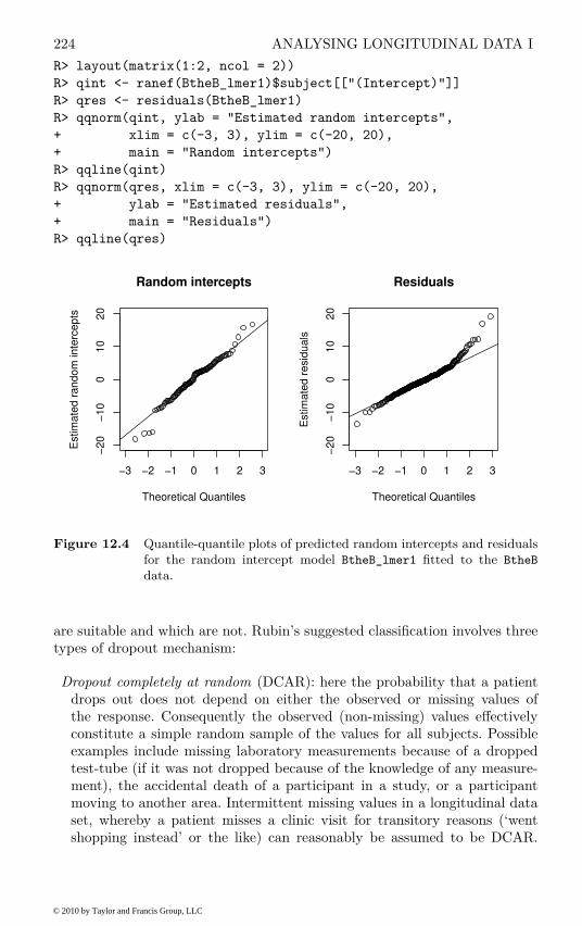
224 ANALYSING LONGITUDINAL DATA I
R> layout(matrix(1:2, ncol = 2))
R> qint <- ranef(BtheB_lmer1)$subject[["(Intercept)"]]
R> qres <- residuals(BtheB_lmer1)
R> qqnorm(qint, ylab = "Estimated random intercepts",
+ xlim = c(-3, 3), ylim = c(-20, 20),
+ main = "Random intercepts")
R> qqline(qint)
R> qqnorm(qres, xlim = c(-3, 3), ylim = c(-20, 20),
+ ylab = "Estimated residuals",
+ main = "Residuals")
R> qqline(qres)
−3 −2 −1 0 1 2 3
−2
0−
10
01
02
0
Random intercepts
Theoretical Quantiles
Estim
ate
d r
an
do
m in
terc
ep
ts
−3 −2 −1 0 1 2 3
−2
0−
10
01
02
0
Residuals
Theoretical Quantiles
Estim
ate
d r
esid
ua
ls
Figure 12.4 Quantile-quantile plots of predicted random intercepts and residualsfor the random intercept model BtheB_lmer1 fitted to the BtheB
data.
are suitable and which are not. Rubin’s suggested classification involves threetypes of dropout mechanism:
Dropout completely at random (DCAR): here the probability that a patientdrops out does not depend on either the observed or missing values ofthe response. Consequently the observed (non-missing) values effectivelyconstitute a simple random sample of the values for all subjects. Possibleexamples include missing laboratory measurements because of a droppedtest-tube (if it was not dropped because of the knowledge of any measure-ment), the accidental death of a participant in a study, or a participantmoving to another area. Intermittent missing values in a longitudinal dataset, whereby a patient misses a clinic visit for transitory reasons (‘wentshopping instead’ or the like) can reasonably be assumed to be DCAR.
© 2010 by Taylor and Francis Group, LLC
THE PROBLEM OF DROPOUTS 225
Completely random dropout causes least problem for data analysis, but itis a strong assumption.
Dropout at random (DAR): The dropout at random mechanism occurs whenthe probability of dropping out depends on the outcome measures thathave been observed in the past, but given this information is conditionallyindependent of all the future (unrecorded) values of the outcome variablefollowing dropout. Here ‘missingness’ depends only on the observed datawith the distribution of future values for a subject who drops out at aparticular time being the same as the distribution of the future values ofa subject who remains in at that time, if they have the same covariatesand the same past history of outcome up to and including the specific timepoint. Murray and Findlay (1988) provide an example of this type of missingvalue from a study of hypertensive drugs in which the outcome measurewas diastolic blood pressure. The protocol of the study specified that theparticipant was to be removed from the study when his/her blood pressuregot too large. Here blood pressure at the time of dropout was observedbefore the participant dropped out, so although the dropout mechanism isnot DCAR since it depends on the values of blood pressure, it is DAR,because dropout depends only on the observed part of the data. A furtherexample of a DAR mechanism is provided by Heitjan (1997), and involvesa study in which the response measure is body mass index (BMI). Supposethat the measure is missing because subjects who had high body massindex values at earlier visits avoided being measured at later visits out ofembarrassment, regardless of whether they had gained or lost weight inthe intervening period. The missing values here are DAR but not DCAR;consequently methods applied to the data that assumed the latter mightgive misleading results (see later discussion).
Non-ignorable (sometimes referred to as informative): The final type of drop-out mechanism is one where the probability of dropping out depends on theunrecorded missing values – observations are likely to be missing when theoutcome values that would have been observed had the patient not droppedout, are systematically higher or lower than usual (corresponding perhapsto their condition becoming worse or improving). A non-medical exampleis when individuals with lower income levels or very high incomes are lesslikely to provide their personal income in an interview. In a medical settingpossible examples are a participant dropping out of a longitudinal studywhen his/her blood pressure became too high and this value was not ob-served, or when their pain become intolerable and we did not record theassociated pain value. For the BDI example introduced above, if subjectswere more likely to avoid being measured if they had put on extra weightsince the last visit, then the data are non-ignorably missing. Dealing withdata containing missing values that result from this type of dropout mech-anism is difficult. The correct analyses for such data must estimate thedependence of the missingness probability on the missing values. Modelsand software that attempt this are available (see, for example, Diggle and
© 2010 by Taylor and Francis Group, LLC
226 ANALYSING LONGITUDINAL DATA I
Kenward, 1994) but their use is not routine and, in addition, it must beremembered that the associated parameter estimates can be unreliable.
Under what type of dropout mechanism are the mixed effects models con-sidered in this chapter valid? The good news is that such models can be shownto give valid results under the relatively weak assumption that the dropoutmechanism is DAR (see Carpenter et al., 2002). When the missing valuesare thought to be informative, any analysis is potentially problematical. ButDiggle and Kenward (1994) have developed a modelling framework for longitu-dinal data with informative dropouts, in which random or completely randomdropout mechanisms are also included as explicit models. The essential featureof the procedure is a logistic regression model for the probability of droppingout, in which the explanatory variables can include previous values of the re-sponse variable, and, in addition, the unobserved value at dropout as a latentvariable (i.e., an unobserved variable). In other words, the dropout probabilityis allowed to depend on both the observed measurement history and the un-observed value at dropout. This allows both a formal assessment of the typeof dropout mechanism in the data, and the estimation of effects of interest,for example, treatment effects under different assumptions about the dropoutmechanism. A full technical account of the model is given in Diggle and Ken-ward (1994) and a detailed example that uses the approach is described inCarpenter et al. (2002).
One of the problems for an investigator struggling to identify the dropoutmechanism in a data set is that there are no routine methods to help, althougha number of largely ad hoc graphical procedures can be used as described inDiggle (1998), Everitt (2002b) and Carpenter et al. (2002). One very simpleprocedure for assessing the dropout mechanism suggested in Carpenter et al.(2002) involves plotting the observations for each treatment group, at eachtime point, differentiating between two categories of patients; those who doand those who do not attend their next scheduled visit. Any clear differencebetween the distributions of values for these two categories indicates thatdropout is not completely at random. For the Beat the Blues data, such aplot is shown in Figure 12.5. When comparing the distribution of BDI valuesfor patients that do (circles) and do not (bullets) attend the next scheduledvisit, there is no apparent difference and so it is reasonable to assume dropoutcompletely at random.
12.7 Summary
Linear mixed effects models are extremely useful for modelling longitudinaldata. The models allow the correlations between the repeated measurementsto be accounted for so that correct inferences can be drawn about the ef-fects of covariates of interest on the repeated response values. In this chapterwe have concentrated on responses that are continuous and conditional on theexplanatory variables and random effects have a normal distribution. But ran-
© 2010 by Taylor and Francis Group, LLC

SUMMARY 227
R> bdi <- BtheB[, grep("bdi", names(BtheB))]
R> plot(1:4, rep(-0.5, 4), type = "n", axes = FALSE,
+ ylim = c(0, 50), xlab = "Months", ylab = "BDI")
R> axis(1, at = 1:4, labels = c(0, 2, 3, 5))
R> axis(2)
R> for (i in 1:4) {
+ dropout <- is.na(bdi[,i + 1])
+ points(rep(i, nrow(bdi)) + ifelse(dropout, 0.05, -0.05),
+ jitter(bdi[,i]), pch = ifelse(dropout, 20, 1))
+ }
Months
BD
I
0 2 3 5
01
02
03
04
05
0
l
l
l
l
l
l
l
l
l
l
l
l
l
l
l
l
l
l
l
l
l
l
l
l
l
l
l
l
l
l
l
l
l
l
l
l
l
l
l
l
l
l
l
l
l
l
l
Figure 12.5 Distribution of BDI values for patients that do (circles) and do not(bullets) attend the next scheduled visit.
© 2010 by Taylor and Francis Group, LLC

228 ANALYSING LONGITUDINAL DATA I
dom effects models can also be applied to non-normal responses, for examplebinary variables – see, for example, Everitt (2002b).
The lack of independence of repeated measures data is what makes themodelling of such data a challenge. But even when only a single measurementof a response is involved, correlation can, in some circumstances, occur be-tween the response values of different individuals and cause similar problems.As an example consider a randomised clinical trial in which subjects are re-cruited at multiple study centres. The multicentre design can help to provideadequate sample sizes and enhance the generalisability of the results. Howeverfactors that vary by centre, including patient characteristics and medical prac-tise patterns, may exert a sufficiently powerful effect to make inferences thatignore the ‘clustering’ seriously misleading. Consequently it may be necessaryto incorporate random effects for centres into the analysis.
Exercises
Ex. 12.1 Use the lm function to fit a model to the Beat the Blues data thatassumes that the repeated measurements are independent. Compare theresults to those from fitting the random intercept model BtheB_lmer1.
Ex. 12.2 Investigate whether there is any evidence of an interaction betweentreatment and time for the Beat the Blues data.
Ex. 12.3 Construct a plot of the mean profiles of both groups in the Beat theBlues data, showing also standard deviation bars at each time point.
Ex. 12.4 The phosphate data given in Table 12.2 show the plasma inorganicphosphate levels for 33 subjects, 20 of whom are controls and 13 of whomhave been classified as obese (Davis, 2002). Produce separate plots of theprofiles of the individuals in each group, and guided by these plots fit whatyou think might be sensible linear mixed effects models.
Table 12.2: phosphate data. Plasma inorganic phosphate levelsfor various time points after glucose challenge.
group t0 t0.5 t1 t1.5 t2 t3 t4 t5
control 4.3 3.3 3.0 2.6 2.2 2.5 3.4 4.4control 3.7 2.6 2.6 1.9 2.9 3.2 3.1 3.9control 4.0 4.1 3.1 2.3 2.9 3.1 3.9 4.0control 3.6 3.0 2.2 2.8 2.9 3.9 3.8 4.0control 4.1 3.8 2.1 3.0 3.6 3.4 3.6 3.7control 3.8 2.2 2.0 2.6 3.8 3.6 3.0 3.5control 3.8 3.0 2.4 2.5 3.1 3.4 3.5 3.7control 4.4 3.9 2.8 2.1 3.6 3.8 4.0 3.9control 5.0 4.0 3.4 3.4 3.3 3.6 4.0 4.3control 3.7 3.1 2.9 2.2 1.5 2.3 2.7 2.8control 3.7 2.6 2.6 2.3 2.9 2.2 3.1 3.9control 4.4 3.7 3.1 3.2 3.7 4.3 3.9 4.8
© 2010 by Taylor and Francis Group, LLC
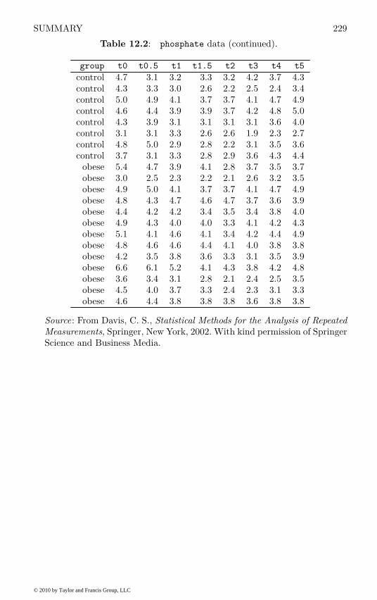
SUMMARY 229
Table 12.2: phosphate data (continued).
group t0 t0.5 t1 t1.5 t2 t3 t4 t5
control 4.7 3.1 3.2 3.3 3.2 4.2 3.7 4.3control 4.3 3.3 3.0 2.6 2.2 2.5 2.4 3.4control 5.0 4.9 4.1 3.7 3.7 4.1 4.7 4.9control 4.6 4.4 3.9 3.9 3.7 4.2 4.8 5.0control 4.3 3.9 3.1 3.1 3.1 3.1 3.6 4.0control 3.1 3.1 3.3 2.6 2.6 1.9 2.3 2.7control 4.8 5.0 2.9 2.8 2.2 3.1 3.5 3.6control 3.7 3.1 3.3 2.8 2.9 3.6 4.3 4.4
obese 5.4 4.7 3.9 4.1 2.8 3.7 3.5 3.7obese 3.0 2.5 2.3 2.2 2.1 2.6 3.2 3.5obese 4.9 5.0 4.1 3.7 3.7 4.1 4.7 4.9obese 4.8 4.3 4.7 4.6 4.7 3.7 3.6 3.9obese 4.4 4.2 4.2 3.4 3.5 3.4 3.8 4.0obese 4.9 4.3 4.0 4.0 3.3 4.1 4.2 4.3obese 5.1 4.1 4.6 4.1 3.4 4.2 4.4 4.9obese 4.8 4.6 4.6 4.4 4.1 4.0 3.8 3.8obese 4.2 3.5 3.8 3.6 3.3 3.1 3.5 3.9obese 6.6 6.1 5.2 4.1 4.3 3.8 4.2 4.8obese 3.6 3.4 3.1 2.8 2.1 2.4 2.5 3.5obese 4.5 4.0 3.7 3.3 2.4 2.3 3.1 3.3obese 4.6 4.4 3.8 3.8 3.8 3.6 3.8 3.8
Source: From Davis, C. S., Statistical Methods for the Analysis of RepeatedMeasurements, Springer, New York, 2002. With kind permission of SpringerScience and Business Media.
© 2010 by Taylor and Francis Group, LLC

CHAPTER 13
Analysing Longitudinal Data II –Generalised Estimation Equations andLinear Mixed Effect Models: Treating
Respiratory Illness and EpilepticSeizures
13.1 Introduction
The data in Table 13.1 were collected in a clinical trial comparing two treat-ments for a respiratory illness (Davis, 1991).
Table 13.1: respiratory data. Randomised clinical trial datafrom patients suffering from respiratory illness. Onlythe data of the first seven patients are shown here.
centre treatment gender age status month subject
1 placebo female 46 poor 0 11 placebo female 46 poor 1 11 placebo female 46 poor 2 11 placebo female 46 poor 3 11 placebo female 46 poor 4 11 placebo female 28 poor 0 21 placebo female 28 poor 1 21 placebo female 28 poor 2 21 placebo female 28 poor 3 21 placebo female 28 poor 4 21 treatment female 23 good 0 31 treatment female 23 good 1 31 treatment female 23 good 2 31 treatment female 23 good 3 31 treatment female 23 good 4 31 placebo female 44 good 0 41 placebo female 44 good 1 41 placebo female 44 good 2 41 placebo female 44 good 3 41 placebo female 44 poor 4 41 placebo male 13 good 0 5
231
© 2010 by Taylor and Francis Group, LLC
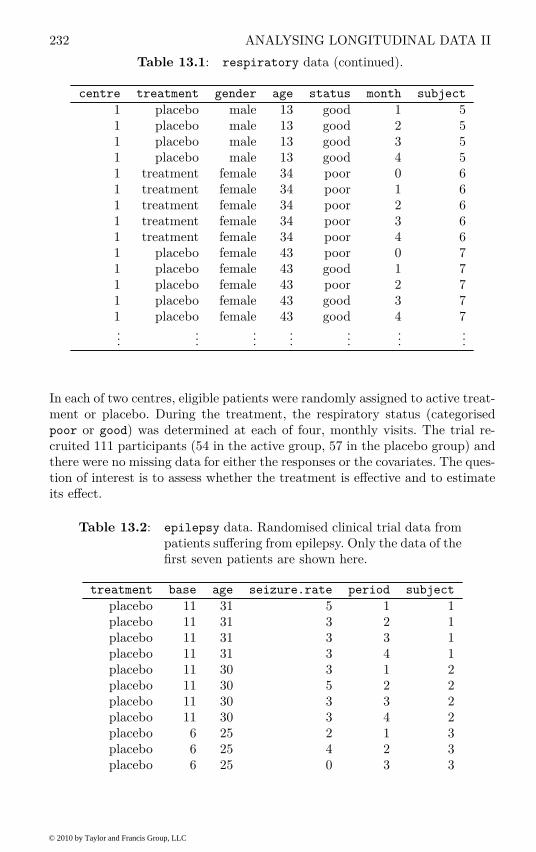
232 ANALYSING LONGITUDINAL DATA II
Table 13.1: respiratory data (continued).
centre treatment gender age status month subject
1 placebo male 13 good 1 51 placebo male 13 good 2 51 placebo male 13 good 3 51 placebo male 13 good 4 51 treatment female 34 poor 0 61 treatment female 34 poor 1 61 treatment female 34 poor 2 61 treatment female 34 poor 3 61 treatment female 34 poor 4 61 placebo female 43 poor 0 71 placebo female 43 good 1 71 placebo female 43 poor 2 71 placebo female 43 good 3 71 placebo female 43 good 4 7...
......
......
......
In each of two centres, eligible patients were randomly assigned to active treat-ment or placebo. During the treatment, the respiratory status (categorisedpoor or good) was determined at each of four, monthly visits. The trial re-cruited 111 participants (54 in the active group, 57 in the placebo group) andthere were no missing data for either the responses or the covariates. The ques-tion of interest is to assess whether the treatment is effective and to estimateits effect.
Table 13.2: epilepsy data. Randomised clinical trial data frompatients suffering from epilepsy. Only the data of thefirst seven patients are shown here.
treatment base age seizure.rate period subject
placebo 11 31 5 1 1placebo 11 31 3 2 1placebo 11 31 3 3 1placebo 11 31 3 4 1placebo 11 30 3 1 2placebo 11 30 5 2 2placebo 11 30 3 3 2placebo 11 30 3 4 2placebo 6 25 2 1 3placebo 6 25 4 2 3placebo 6 25 0 3 3
© 2010 by Taylor and Francis Group, LLC

METHODS FOR NON-NORMAL DISTRIBUTIONS 233
Table 13.2: epilepsy data (continued).
treatment base age seizure.rate period subject
placebo 6 25 5 4 3placebo 8 36 4 1 4placebo 8 36 4 2 4placebo 8 36 1 3 4placebo 8 36 4 4 4placebo 66 22 7 1 5placebo 66 22 18 2 5placebo 66 22 9 3 5placebo 66 22 21 4 5placebo 27 29 5 1 6placebo 27 29 2 2 6placebo 27 29 8 3 6placebo 27 29 7 4 6placebo 12 31 6 1 7placebo 12 31 4 2 7placebo 12 31 0 3 7placebo 12 31 2 4 7
......
......
......
In a clinical trial reported by Thall and Vail (1990), 59 patients with epilepsywere randomised to groups receiving either the antiepileptic drug Progabideor a placebo in addition to standard chemotherapy. The numbers of seizuressuffered in each of four, two-week periods were recorded for each patient alongwith a baseline seizure count for the 8 weeks prior to being randomised totreatment and age. The main question of interest is whether taking Progabidereduced the number of epileptic seizures compared with placebo. A subset ofthe data is given in Table 13.2.
Note that the two data sets are shown in their ‘long form’ i.e., one measure-ment per row in the corresponding data.frames.
13.2 Methods for Non-normal Distributions
The data sets respiratory and epilepsy arise from longitudinal clinical tri-als, the same type of study that was the subject of consideration in Chapter 12.But in each case the repeatedly measured response variable is clearly not nor-mally distributed making the models considered in the previous chapter un-suitable. In Table 13.1 we have a binary response observed on four occasions,and in Table 13.2 a count response also observed on four occasions. If wechoose to ignore the repeated measurements aspects of the two data sets wecould use the methods of Chapter 7 applied to the data arranged in the ‘long’
© 2010 by Taylor and Francis Group, LLC

234 ANALYSING LONGITUDINAL DATA II
form introduced in Chapter 12. For the respiratory data in Table 13.1 wecould then apply logistic regression and for epilepsy in Table 13.2, Poissonregression. It can be shown that this approach will give consistent estimates ofthe regression coefficients, i.e., with large samples these point estimates shouldbe close to the true population values. But the assumption of the independenceof the repeated measurements will lead to estimated standard errors that aretoo small for the between-subjects covariates (at least when the correlationbetween the repeated measurements are positive) as a result of assuming thatthere are more independent data points than are justified.
We might begin by asking if there is something relatively simple that canbe done to ‘fix-up’ these standard errors so that we can still apply the R
glm function to get reasonably satisfactory results on longitudinal data witha non-normal response? Two approaches which can often help to get moresuitable estimates of the required standard errors are bootstrapping and useof the robust/sandwich, Huber-White variance estimator.
The idea underlying the bootstrap (see Chapter 8 and Chapter 9), a tech-nique described in detail in Efron and Tibshirani (1993), is to resample fromthe observed data with replacement to achieve a sample of the same size eachtime, and to use the variation in the estimated parameters across the set ofbootstrap samples in order to get a value for the sampling variability of theestimate (see Chapter 8 also). With correlated data, the bootstrap sampleneeds to be drawn with replacement from the set of independent subjects, sothat intra-subject correlation is preserved in the bootstrap samples. We shallnot consider this approach any further here.
The sandwich or robust estimate of variance (see Everitt and Pickles, 2000,for complete details including an explicit definition), involves, unlike the boot-strap which is computationally intensive, a closed-form calculation, based onan asymptotic (large-sample) approximation; it is known to provide good re-sults in many situations. We shall illustrate its use in later examples.
But perhaps more satisfactory would be an approach that fully utilises in-formation on the data’s structure, including dependencies over time. In thelinear mixed models for Gaussian responses described in Chapter 12, estima-tion of the regression parameters linking explanatory variables to the responsevariable and their standard errors needed to take account of the correlationalstructure of the data, but their interpretation could be undertaken indepen-dent of this structure. When modelling non-normal responses this indepen-dence of estimation and interpretation no longer holds. Different assumptionsabout how the correlations are generated can lead to regression coefficientswith different interpretations. The essential difference is between marginalmodels and conditional models.
13.2.1 Marginal Models
Longitudinal data can be considered as a series of cross-sections, and marginalmodels for such data use the generalised linear model (see Chapter 7) to fit
© 2010 by Taylor and Francis Group, LLC
METHODS FOR NON-NORMAL DISTRIBUTIONS 235
each cross-section. In this approach the relationship of the marginal meanand the explanatory variables is modelled separately from the within-subjectcorrelation. The marginal regression coefficients have the same interpretationas coefficients from a cross-sectional analysis, and marginal models are naturalanalogues for correlated data of generalised linear models for independentdata. Fitting marginal models to non-normal longitudinal data involves the useof a procedure known as generalised estimating equations (GEE), introducedby Liang and Zeger (1986). This approach may be viewed as a multivariateextension of the generalised linear model and the quasi-likelihood method (seeChapter 7). But the problem with applying a direct analogue of the generalisedlinear model to longitudinal data with non-normal responses is that thereis usually no suitable likelihood function with the required combination ofthe appropriate link function, error distribution and correlation structure. Toovercome this problem Liang and Zeger (1986) introduced a general methodfor incorporating within-subject correlation in GLMs, which is essentially anextension of the quasi-likelihood approach mentioned briefly in Chapter 7. Asin conventional generalised linear models, the variances of the responses giventhe covariates are assumed to be of the form Var(response) = φV(µ) wherethe variance function V (µ) is determined by the choice of distribution family(see Chapter 7). Since overdispersion is common in longitudinal data, thedispersion parameter φ is typically estimated even if the distribution requiresφ = 1. The feature of these generalised estimation equations that differs fromthe usual generalised linear model is that different responses on the sameindividual are allowed to be correlated given the covariates. These correlationsare assumed to have a relatively simple structure defined by a small numberof parameters. The following correlation structures are commonly used (Yij
represents the value of the jth repeated measurement of the response variableon subject i).
An identity matrix leading to the independence working model in whichthe generalised estimating equation reduces to the univariate estimatingequation given in Chapter 7, obtained by assuming that the repeated mea-surements are independent.
An exchangeable correlation matrix with a single parameter similar tothat described in Chapter 12. Here the correlation between each pair ofrepeated measurements is assumed to be the same, i.e., corr(Yij , Yik) = ρ.
An AR-1 autoregressive correlation matrix, also with a single param-eter, but in which corr(Yij , Yik) = ρ|k−j|, j 6= k. This can allow the cor-relations of measurements taken farther apart to be less than those takencloser to one another.
An unstructured correlation matrix with K(K−1)/2 parameters whereK is the number of repeated measurements andcorr(Yij , Yjk) = ρjk
For given values of the regression parameters β1, . . . βq, the ρ-parametersof the working correlation matrix can be estimated along with the dispersionparameter φ (see Zeger and Liang, 1986, for details). These estimates can then
© 2010 by Taylor and Francis Group, LLC
236 ANALYSING LONGITUDINAL DATA II
be used in the so-called generalised estimating equations to obtain estimatesof the regression parameters. The GEE algorithm proceeds by iterating be-tween (1) estimation of the regression parameters using the correlation anddispersion parameters from the previous iteration and (2) estimation of thecorrelation and dispersion parameters using the regression parameters fromthe previous iteration.
The estimated regression coefficients are ‘robust’ in the sense that they areconsistent from misspecified correlation structures assuming that the meanstructure is correctly specified. Note however that the GEE estimates of mar-ginal effects are not robust against misspecified regression structures, such asomitted covariates.
The use of GEE estimation on a longitudinal data set in which some subjectsdrop out assumes that they drop out completely at random (see Chapter 12).
13.2.2 Conditional Models
The random effects approach described in the previous chapter can be ex-tended to non-normal responses although the resulting models can be difficultto estimate because the likelihood involves integrals over the random effectsdistribution that generally do not have closed forms. A consequence is that itis often possible to fit only relatively simple models. In these models estimatedregression coefficients have to be interpreted, conditional on the random ef-fects. The regression parameters in the model are said to be subject-specificand such effects will differ from the marginal or population averaged effects es-timated using GEE, except when using an identity link function and a normalerror distribution.
Consider a set of longitudinal data in which Yij is the value of a binaryresponse for individual i at say time tj . The logistic regression model (seeChapter 7) for the response is now written as
logit (P(yij = 1|ui)) = β0 + β1tj + ui (13.1)
where ui is a random effect assumed to be normally distributed with zeromean and variance σ2
u. This is a simple example of a generalised linear mixedmodel because it is a generalised linear model with both a fixed effect, β1, anda random effect, ui.
Here the regression parameter β1 again represents the change in the log oddsper unit change in time, but this is now conditional on the random effect. Wecan illustrate this difference graphically by simulating the model (13.1); theresult is shown in Figure 13.1. Here the thin grey curves represent subject-specific relationships between the probability that the response equals one anda covariate t for model (13.1). The horizontal shifts are due to different valuesof the random intercept. The thick black curve represents the population av-eraged relationship, formed by averaging the thin curves for each value of t. Itis, in effect, the thick curve that would be estimated in a marginal model (see
© 2010 by Taylor and Francis Group, LLC
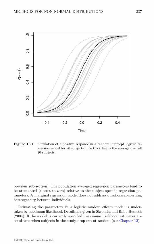
METHODS FOR NON-NORMAL DISTRIBUTIONS 237
−0.4 −0.2 0.0 0.2 0.4
0.0
0.2
0.4
0.6
0.8
1.0
Time
P((y
==1))
Figure 13.1 Simulation of a positive response in a random intercept logistic re-
gression model for 20 subjects. The thick line is the average over all
20 subjects.
previous sub-section). The population averaged regression parameters tend tobe attenuated (closest to zero) relative to the subject-specific regression pa-rameters. A marginal regression model does not address questions concerningheterogeneity between individuals.
Estimating the parameters in a logistic random effects model is under-taken by maximum likelihood. Details are given in Skrondal and Rabe-Hesketh(2004). If the model is correctly specified, maximum likelihood estimates areconsistent when subjects in the study drop out at random (see Chapter 12).
© 2010 by Taylor and Francis Group, LLC

238 ANALYSING LONGITUDINAL DATA II
13.3 Analysis Using R: GEE
13.3.1 Beat the Blues Revisited
Although we have introduced GEE as a method for analysing longitudinaldata where the response variable is non-normal, it can also be applied to datawhere the response can be assumed to follow a conditional normal distribution(conditioning being on the explanatory variables). Consequently we first applythe method to the data used in the previous chapter so we can compare theresults we get with those obtained from using the mixed-effects models usedthere.
To use the gee function, package gee (Carey et al., 2008) has to be installedand attached:
R> library("gee")
The gee function is used in a similar way to the lme function met in Chapter 12with the addition of the features of the glm function that specify the appro-priate error distribution for the response and the implied link function, andan argument to specify the structure of the working correlation matrix. Herewe will fit an independence structure and then an exchangeable structure.The R code for fitting generalised estimation equations to the BtheB_long
data (as constructed in Chapter 12) with identity working correlation matrixis as follows (note that the gee function assumes the rows of the data.frameBtheB_long to be ordered with respect to subjects):
R> osub <- order(as.integer(BtheB_long$subject))
R> BtheB_long <- BtheB_long[osub,]
R> btb_gee <- gee(bdi ~ bdi.pre + trt + length + drug,
+ data = BtheB_long, id = subject, family = gaussian,
+ corstr = "independence")
and with exchangeable correlation matrix:
R> btb_gee1 <- gee(bdi ~ bdi.pre + trt + length + drug,
+ data = BtheB_long, id = subject, family = gaussian,
+ corstr = "exchangeable")
The summary method can be used to inspect the fitted models; the results areshown in Figures 13.2 and 13.3.
Note how the naıve and the sandwich or robust estimates of the standarderrors are considerably different for the independence structure (Figure 13.2),but quite similar for the exchangeable structure (Figure 13.3). This simplyreflects that using an exchangeable working correlation matrix is more realisticfor these data and that the standard errors resulting from this assumption arealready quite reasonable without applying the ‘sandwich’ procedure to them.And if we compare the results under this assumed structure with those forthe random intercept model given in Chapter 12 (Figure 12.2) we see thatthey are almost identical, since the random intercept model also implies anexchangeable structure for the correlations of the repeated measurements.
The single estimated parameter for the working correlation matrix from the
© 2010 by Taylor and Francis Group, LLC

ANALYSIS USING R: GEE 239
R> summary(btb_gee)
...
Model:
Link: Identity
Variance to Mean Relation: Gaussian
Correlation Structure: Independent
...
Coefficients:
Estimate Naive S.E. Naive z Robust S.E. Robust z
(Intercept) 3.569 1.4833 2.41 2.2695 1.572
bdi.pre 0.582 0.0564 10.32 0.0916 6.355
trtBtheB -3.237 1.1296 -2.87 1.7746 -1.824
length>6m 1.458 1.1380 1.28 1.4826 0.983
drugYes -3.741 1.1766 -3.18 1.7827 -2.099
Estimated Scale Parameter: 79.3
...
Figure 13.2 R output of the summary method for the btb_gee model (slightly
abbreviated).
GEE procedure is 0.676, very similar to the estimated intra-class correlationcoefficient from the random intercept model. i.e., 7.032/(5.072 + 7.032) = 0.66– see Figure 12.2.
13.3.2 Respiratory Illness
We will now apply the GEE procedure to the respiratory data shown inTable 13.1. Given the binary nature of the response variable we will choosea binomial error distribution and by default a logistic link function. We shallalso fix the scale parameter φ described in Chapter 7 at one. (The defaultin the gee function is to estimate this parameter.) Again we will apply theprocedure twice, firstly with an independence structure and then with anexchangeable structure for the working correlation matrix. We will also fit alogistic regression model to the data using glm so we can compare results.
The baseline status, i.e., the status for month == 0, will enter the mod-els as an explanatory variable and thus we have to rearrange the data.framerespiratory in order to create a new variable baseline:
R> data("respiratory", package = "HSAUR2")
R> resp <- subset(respiratory, month > "0")
R> resp$baseline <- rep(subset(respiratory, month == "0")$status,
+ rep(4, 111))
© 2010 by Taylor and Francis Group, LLC

240 ANALYSING LONGITUDINAL DATA II
R> summary(btb_gee1)
...
Model:
Link: Identity
Variance to Mean Relation: Gaussian
Correlation Structure: Exchangeable
...
Coefficients:
Estimate Naive S.E. Naive z Robust S.E. Robust z
(Intercept) 3.023 2.3039 1.3122 2.2320 1.3544
bdi.pre 0.648 0.0823 7.8741 0.0835 7.7583
trtBtheB -2.169 1.7664 -1.2281 1.7361 -1.2495
length>6m -0.111 1.7309 -0.0643 1.5509 -0.0718
drugYes -3.000 1.8257 -1.6430 1.7316 -1.7323
Estimated Scale Parameter: 81.7
...
Figure 13.3 R output of the summary method for the btb_gee1 model (slightly
abbreviated).
R> resp$nstat <- as.numeric(resp$status == "good")
R> resp$month <- resp$month[, drop = TRUE]
The new variable nstat is simply a dummy coding for a poor respiratorystatus. Now we can use the data resp to fit a logistic regression model andGEE models with an independent and an exchangeable correlation structureas follows.
R> resp_glm <- glm(status ~ centre + trt + gender + baseline
+ + age, data = resp, family = "binomial")
R> resp_gee1 <- gee(nstat ~ centre + trt + gender + baseline
+ + age, data = resp, family = "binomial", id = subject,
+ corstr = "independence", scale.fix = TRUE,
+ scale.value = 1)
R> resp_gee2 <- gee(nstat ~ centre + trt + gender + baseline
+ + age, data = resp, family = "binomial", id = subject,
+ corstr = "exchangeable", scale.fix = TRUE,
+ scale.value = 1)
Again, summary methods can be used for an inspection of the details of thefitted models; the results are given in Figures 13.4, 13.5 and 13.6. We see thatthe results from applying logistic regression to the data with the glm func-tion gives identical results to those obtained from gee with an independencecorrelation structure (comparing the glm standard errors with the naıve stan-dard errors from gee). The robust standard errors for the between subject
© 2010 by Taylor and Francis Group, LLC
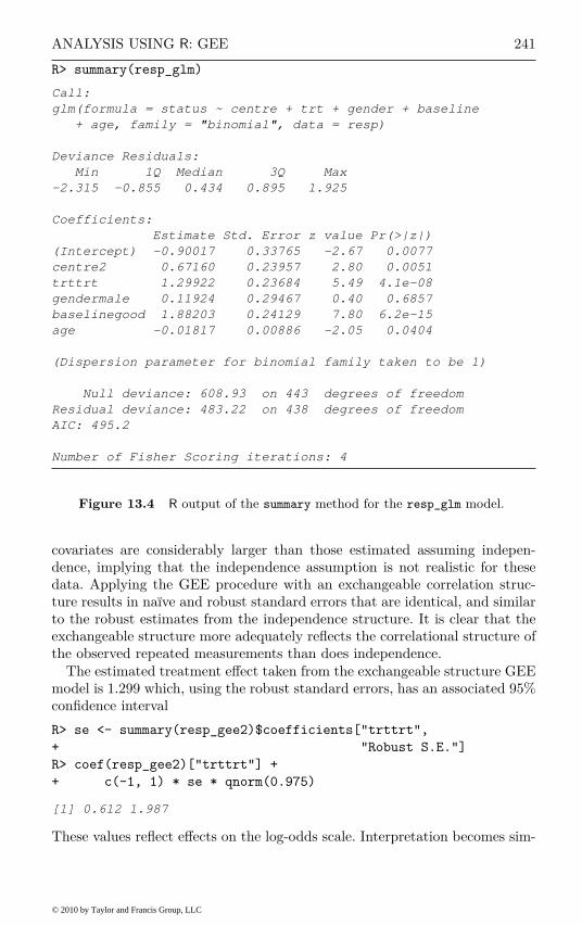
ANALYSIS USING R: GEE 241
R> summary(resp_glm)
Call:
glm(formula = status ~ centre + trt + gender + baseline
+ age, family = "binomial", data = resp)
Deviance Residuals:
Min 1Q Median 3Q Max
-2.315 -0.855 0.434 0.895 1.925
Coefficients:
Estimate Std. Error z value Pr(>|z|)
(Intercept) -0.90017 0.33765 -2.67 0.0077
centre2 0.67160 0.23957 2.80 0.0051
trttrt 1.29922 0.23684 5.49 4.1e-08
gendermale 0.11924 0.29467 0.40 0.6857
baselinegood 1.88203 0.24129 7.80 6.2e-15
age -0.01817 0.00886 -2.05 0.0404
(Dispersion parameter for binomial family taken to be 1)
Null deviance: 608.93 on 443 degrees of freedom
Residual deviance: 483.22 on 438 degrees of freedom
AIC: 495.2
Number of Fisher Scoring iterations: 4
Figure 13.4 R output of the summary method for the resp_glm model.
covariates are considerably larger than those estimated assuming indepen-dence, implying that the independence assumption is not realistic for thesedata. Applying the GEE procedure with an exchangeable correlation struc-ture results in naıve and robust standard errors that are identical, and similarto the robust estimates from the independence structure. It is clear that theexchangeable structure more adequately reflects the correlational structure ofthe observed repeated measurements than does independence.
The estimated treatment effect taken from the exchangeable structure GEEmodel is 1.299 which, using the robust standard errors, has an associated 95%confidence interval
R> se <- summary(resp_gee2)$coefficients["trttrt",
+ "Robust S.E."]
R> coef(resp_gee2)["trttrt"] +
+ c(-1, 1) * se * qnorm(0.975)
[1] 0.612 1.987
These values reflect effects on the log-odds scale. Interpretation becomes sim-
© 2010 by Taylor and Francis Group, LLC
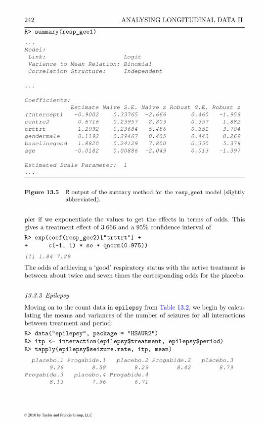
242 ANALYSING LONGITUDINAL DATA II
R> summary(resp_gee1)
...
Model:
Link: Logit
Variance to Mean Relation: Binomial
Correlation Structure: Independent
...
Coefficients:
Estimate Naive S.E. Naive z Robust S.E. Robust z
(Intercept) -0.9002 0.33765 -2.666 0.460 -1.956
centre2 0.6716 0.23957 2.803 0.357 1.882
trttrt 1.2992 0.23684 5.486 0.351 3.704
gendermale 0.1192 0.29467 0.405 0.443 0.269
baselinegood 1.8820 0.24129 7.800 0.350 5.376
age -0.0182 0.00886 -2.049 0.013 -1.397
Estimated Scale Parameter: 1
...
Figure 13.5 R output of the summary method for the resp_gee1 model (slightly
abbreviated).
pler if we exponentiate the values to get the effects in terms of odds. Thisgives a treatment effect of 3.666 and a 95% confidence interval of
R> exp(coef(resp_gee2)["trttrt"] +
+ c(-1, 1) * se * qnorm(0.975))
[1] 1.84 7.29
The odds of achieving a ‘good’ respiratory status with the active treatment isbetween about twice and seven times the corresponding odds for the placebo.
13.3.3 Epilepsy
Moving on to the count data in epilepsy from Table 13.2, we begin by calcu-lating the means and variances of the number of seizures for all interactionsbetween treatment and period:
R> data("epilepsy", package = "HSAUR2")
R> itp <- interaction(epilepsy$treatment, epilepsy$period)
R> tapply(epilepsy$seizure.rate, itp, mean)
placebo.1 Progabide.1 placebo.2 Progabide.2 placebo.3
9.36 8.58 8.29 8.42 8.79
Progabide.3 placebo.4 Progabide.4
8.13 7.96 6.71
© 2010 by Taylor and Francis Group, LLC
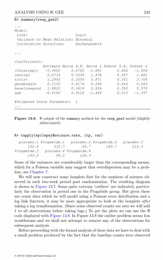
ANALYSIS USING R: GEE 243
R> summary(resp_gee2)
...
Model:
Link: Logit
Variance to Mean Relation: Binomial
Correlation Structure: Exchangeable
...
Coefficients:
Estimate Naive S.E. Naive z Robust S.E. Robust z
(Intercept) -0.9002 0.4785 -1.881 0.460 -1.956
centre2 0.6716 0.3395 1.978 0.357 1.882
trttrt 1.2992 0.3356 3.871 0.351 3.704
gendermale 0.1192 0.4176 0.286 0.443 0.269
baselinegood 1.8820 0.3419 5.504 0.350 5.376
age -0.0182 0.0126 -1.446 0.013 -1.397
Estimated Scale Parameter: 1
...
Figure 13.6 R output of the summary method for the resp_gee2 model (slightly
abbreviated).
R> tapply(epilepsy$seizure.rate, itp, var)
placebo.1 Progabide.1 placebo.2 Progabide.2 placebo.3
102.8 332.7 66.7 140.7 215.3
Progabide.3 placebo.4 Progabide.4
193.0 58.2 126.9
Some of the variances are considerably larger than the corresponding means,which for a Poisson variable may suggest that overdispersion may be a prob-lem, see Chapter 7.
We will now construct some boxplots first for the numbers of seizures ob-served in each two-week period post randomisation. The resulting diagramis shown in Figure 13.7. Some quite extreme ‘outliers’ are indicated, particu-larly the observation in period one in the Progabide group. But given theseare count data which we will model using a Poisson error distribution and alog link function, it may be more appropriate to look at the boxplots aftertaking a log transformation. (Since some observed counts are zero we will add1 to all observations before taking logs.) To get the plots we can use the R
code displayed with Figure 13.8. In Figure 13.8 the outlier problem seems lesstroublesome and we shall not attempt to remove any of the observations forsubsequent analysis.
Before proceeding with the formal analysis of these data we have to deal witha small problem produced by the fact that the baseline counts were observed
© 2010 by Taylor and Francis Group, LLC
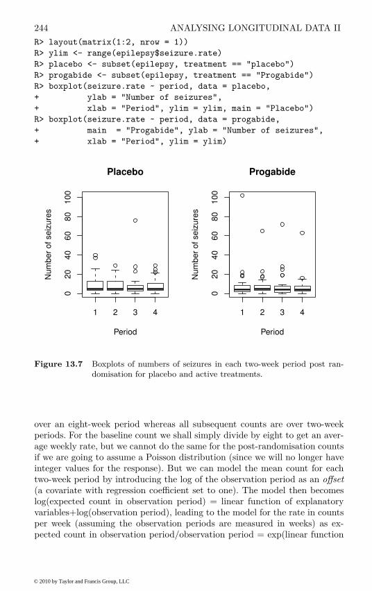
244 ANALYSING LONGITUDINAL DATA II
R> layout(matrix(1:2, nrow = 1))
R> ylim <- range(epilepsy$seizure.rate)
R> placebo <- subset(epilepsy, treatment == "placebo")
R> progabide <- subset(epilepsy, treatment == "Progabide")
R> boxplot(seizure.rate ~ period, data = placebo,
+ ylab = "Number of seizures",
+ xlab = "Period", ylim = ylim, main = "Placebo")
R> boxplot(seizure.rate ~ period, data = progabide,
+ main = "Progabide", ylab = "Number of seizures",
+ xlab = "Period", ylim = ylim)
1 2 3 4
02
04
06
08
01
00
Placebo
Period
Nu
mb
er
of
se
izu
res
1 2 3 4
02
04
06
08
01
00
Progabide
Period
Nu
mb
er
of
se
izu
res
Figure 13.7 Boxplots of numbers of seizures in each two-week period post ran-
domisation for placebo and active treatments.
over an eight-week period whereas all subsequent counts are over two-weekperiods. For the baseline count we shall simply divide by eight to get an aver-age weekly rate, but we cannot do the same for the post-randomisation countsif we are going to assume a Poisson distribution (since we will no longer haveinteger values for the response). But we can model the mean count for eachtwo-week period by introducing the log of the observation period as an offset(a covariate with regression coefficient set to one). The model then becomeslog(expected count in observation period) = linear function of explanatoryvariables+log(observation period), leading to the model for the rate in countsper week (assuming the observation periods are measured in weeks) as ex-pected count in observation period/observation period = exp(linear function
© 2010 by Taylor and Francis Group, LLC

ANALYSIS USING R: GEE 245
R> layout(matrix(1:2, nrow = 1))
R> ylim <- range(log(epilepsy$seizure.rate + 1))
R> boxplot(log(seizure.rate + 1) ~ period, data = placebo,
+ main = "Placebo", ylab = "Log number of seizures",
+ xlab = "Period", ylim = ylim)
R> boxplot(log(seizure.rate + 1) ~ period, data = progabide,
+ main = "Progabide", ylab = "Log number of seizures",
+ xlab = "Period", ylim = ylim)
1 2 3 4
01
23
4
Placebo
Period
Lo
g n
um
be
r o
f se
izu
res
1 2 3 4
01
23
4
Progabide
Period
Lo
g n
um
be
r o
f se
izu
res
Figure 13.8 Boxplots of log of numbers of seizures in each two-week period post
randomisation for placebo and active treatments.
of explanatory variables). In our example the observation period is two weeks,so we simply need to set log(2) for each observation as the offset.
We can now fit a Poisson regression model to the data assuming indepen-dence using the glm function. We also use the GEE approach to fit an inde-pendence structure, followed by an exchangeable structure using the followingR code:
R> per <- rep(log(2),nrow(epilepsy))
R> epilepsy$period <- as.numeric(epilepsy$period)
R> names(epilepsy)[names(epilepsy) == "treatment"] <- "trt"
R> fm <- seizure.rate ~ base + age + trt + offset(per)
R> epilepsy_glm <- glm(fm, data = epilepsy, family = "poisson")
R> epilepsy_gee1 <- gee(fm, data = epilepsy, family = "poisson",
+ id = subject, corstr = "independence", scale.fix = TRUE,
+ scale.value = 1)
© 2010 by Taylor and Francis Group, LLC
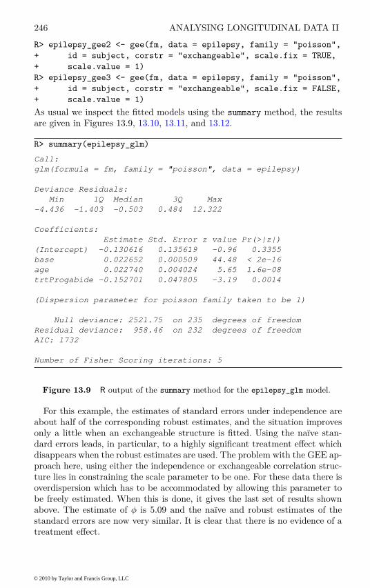
246 ANALYSING LONGITUDINAL DATA II
R> epilepsy_gee2 <- gee(fm, data = epilepsy, family = "poisson",
+ id = subject, corstr = "exchangeable", scale.fix = TRUE,
+ scale.value = 1)
R> epilepsy_gee3 <- gee(fm, data = epilepsy, family = "poisson",
+ id = subject, corstr = "exchangeable", scale.fix = FALSE,
+ scale.value = 1)
As usual we inspect the fitted models using the summary method, the resultsare given in Figures 13.9, 13.10, 13.11, and 13.12.
R> summary(epilepsy_glm)
Call:
glm(formula = fm, family = "poisson", data = epilepsy)
Deviance Residuals:
Min 1Q Median 3Q Max
-4.436 -1.403 -0.503 0.484 12.322
Coefficients:
Estimate Std. Error z value Pr(>|z|)
(Intercept) -0.130616 0.135619 -0.96 0.3355
base 0.022652 0.000509 44.48 < 2e-16
age 0.022740 0.004024 5.65 1.6e-08
trtProgabide -0.152701 0.047805 -3.19 0.0014
(Dispersion parameter for poisson family taken to be 1)
Null deviance: 2521.75 on 235 degrees of freedom
Residual deviance: 958.46 on 232 degrees of freedom
AIC: 1732
Number of Fisher Scoring iterations: 5
Figure 13.9 R output of the summary method for the epilepsy_glm model.
For this example, the estimates of standard errors under independence areabout half of the corresponding robust estimates, and the situation improvesonly a little when an exchangeable structure is fitted. Using the naıve stan-dard errors leads, in particular, to a highly significant treatment effect whichdisappears when the robust estimates are used. The problem with the GEE ap-proach here, using either the independence or exchangeable correlation struc-ture lies in constraining the scale parameter to be one. For these data there isoverdispersion which has to be accommodated by allowing this parameter tobe freely estimated. When this is done, it gives the last set of results shownabove. The estimate of φ is 5.09 and the naıve and robust estimates of thestandard errors are now very similar. It is clear that there is no evidence of atreatment effect.
© 2010 by Taylor and Francis Group, LLC

ANALYSIS USING R: RANDOM EFFECTS 247
R> summary(epilepsy_gee1)
...
Model:
Link: Logarithm
Variance to Mean Relation: Poisson
Correlation Structure: Independent
...
Coefficients:
Estimate Naive S.E. Naive z Robust S.E. Robust z
(Intercept) -0.1306 0.135619 -0.963 0.36515 -0.358
base 0.0227 0.000509 44.476 0.00124 18.332
age 0.0227 0.004024 5.651 0.01158 1.964
trtProgabide -0.1527 0.047805 -3.194 0.17111 -0.892
Estimated Scale Parameter: 1
...
Figure 13.10 R output of the summary method for the epilepsy_gee1 model
(slightly abbreviated).
13.4 Analysis Using R: Random Effects
As an example of using generalised mixed models for the analysis of longitu-dinal data with a non-normal response, the following logistic model will befitted to the respiratory illness data
logit(P(status = good)) = β0 + β1treatment + β2time + β3gender
+β4age + β5centre + β6baseline + u
where u is a subject specific random effect.The necessary R code for fitting the model using the lmer function from
package lme4 (Bates and Sarkar, 2008, Bates, 2005) is:
R> library("lme4")
R> resp_lmer <- lmer(status ~ baseline + month +
+ trt + gender + age + centre + (1 | subject),
+ family = binomial(), data = resp)
R> exp(fixef(resp_lmer))
(Intercept) baselinegood month.L month.Q
0.189 22.361 0.796 0.962
month.C trttrt gendermale age
0.691 8.881 1.227 0.975
centre2
2.875
The significance of the effects as estimated by this random effects model
© 2010 by Taylor and Francis Group, LLC
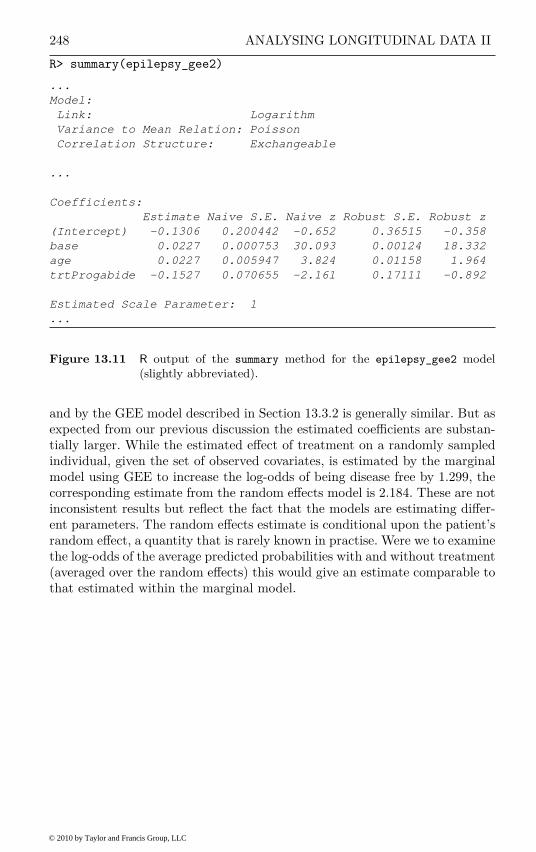
248 ANALYSING LONGITUDINAL DATA II
R> summary(epilepsy_gee2)
...
Model:
Link: Logarithm
Variance to Mean Relation: Poisson
Correlation Structure: Exchangeable
...
Coefficients:
Estimate Naive S.E. Naive z Robust S.E. Robust z
(Intercept) -0.1306 0.200442 -0.652 0.36515 -0.358
base 0.0227 0.000753 30.093 0.00124 18.332
age 0.0227 0.005947 3.824 0.01158 1.964
trtProgabide -0.1527 0.070655 -2.161 0.17111 -0.892
Estimated Scale Parameter: 1
...
Figure 13.11 R output of the summary method for the epilepsy_gee2 model
(slightly abbreviated).
and by the GEE model described in Section 13.3.2 is generally similar. But asexpected from our previous discussion the estimated coefficients are substan-tially larger. While the estimated effect of treatment on a randomly sampledindividual, given the set of observed covariates, is estimated by the marginalmodel using GEE to increase the log-odds of being disease free by 1.299, thecorresponding estimate from the random effects model is 2.184. These are notinconsistent results but reflect the fact that the models are estimating differ-ent parameters. The random effects estimate is conditional upon the patient’srandom effect, a quantity that is rarely known in practise. Were we to examinethe log-odds of the average predicted probabilities with and without treatment(averaged over the random effects) this would give an estimate comparable tothat estimated within the marginal model.
© 2010 by Taylor and Francis Group, LLC

ANALYSIS USING R: RANDOM EFFECTS 249
R> summary(epilepsy_gee3)
...
Model:
Link: Logarithm
Variance to Mean Relation: Poisson
Correlation Structure: Exchangeable
...
Coefficients:
Estimate Naive S.E. Naive z Robust S.E. Robust z
(Intercept) -0.1306 0.45220 -0.289 0.36515 -0.358
base 0.0227 0.00170 13.339 0.00124 18.332
age 0.0227 0.01342 1.695 0.01158 1.964
trtProgabide -0.1527 0.15940 -0.958 0.17111 -0.892
Estimated Scale Parameter: 5.09
...
Figure 13.12 R output of the summary method for the epilepsy_gee3 model
(slightly abbreviated).
R> summary(resp_lmer)
...
Fixed effects:
Estimate Std. Error z value Pr(>|z|)
(Intercept) -1.6666 0.7671 -2.17 0.03
baselinegood 3.1073 0.5325 5.84 5.4e-09
month.L -0.2279 0.2719 -0.84 0.40
month.Q -0.0389 0.2716 -0.14 0.89
month.C -0.3689 0.2727 -1.35 0.18
trttrt 2.1839 0.5237 4.17 3.0e-05
gendermale 0.2045 0.6688 0.31 0.76
age -0.0257 0.0202 -1.27 0.20
centre2 1.0561 0.5381 1.96 0.05
...
Figure 13.13 R output of the summary method for the resp_lmer model (abbre-
viated).
© 2010 by Taylor and Francis Group, LLC

250 ANALYSING LONGITUDINAL DATA II
13.5 Summary
This chapter has outlined and illustrated two approaches to the analysis ofnon-normal longitudinal data: the marginal approach and the random effect(mixed modelling) approach. Though less unified than the methods availablefor normally distributed responses, these methods provide powerful and flex-ible tools to analyse, what until relatively recently, have been seen as almostintractable data.
Exercises
Ex. 13.1 For the epilepsy data investigate what Poisson models are mostsuitable when subject 49 is excluded from the analysis.
Ex. 13.2 Investigate the use of other correlational structures than the in-dependence and exchangeable structures used in the text, for both therespiratory and the epilepsy data.
Ex. 13.3 The data shown in Table 13.3 were collected in a follow-up studyof women patients with schizophrenia (Davis, 2002). The binary responserecorded at 0, 2, 6, 8 and 10 months after hospitalisation was thoughtdisorder (absent or present). The single covariate is the factor indicatingwhether a patient had suffered early or late onset of her condition (age ofonset less than 20 years or age of onset 20 years or above). The questionof interest is whether the course of the illness differs between patients withearly and late onset? Investigate this question using the GEE approach.
© 2010 by Taylor and Francis Group, LLC

SUMMARY 251
Table 13.3: schizophrenia2 data. Clinical trial data from pa-tients suffering from schizophrenia. Only the data ofthe first four patients are shown here.
subject onset disorder month
1 < 20 yrs present 01 < 20 yrs present 21 < 20 yrs absent 61 < 20 yrs absent 81 < 20 yrs absent 102 > 20 yrs absent 02 > 20 yrs absent 22 > 20 yrs absent 62 > 20 yrs absent 82 > 20 yrs absent 103 < 20 yrs present 03 < 20 yrs present 23 < 20 yrs absent 63 < 20 yrs absent 83 < 20 yrs absent 104 < 20 yrs absent 04 < 20 yrs absent 24 < 20 yrs absent 64 < 20 yrs absent 84 < 20 yrs absent 10...
......
...
Source: From Davis, C. S., Statistical Methods for the Analysis of RepeatedMeasurements, Springer, New York, 2002. With kind permission of SpringerScience and Business Media.
© 2010 by Taylor and Francis Group, LLC

CHAPTER 14
Simultaneous Inference and MultipleComparisons: Genetic Components ofAlcoholism, Deer Browsing Intensities,
and Cloud Seeding
14.1 Introduction
Various studies have linked alcohol dependence phenotypes to chromosome 4.One candidate gene is NACP (non-amyloid component of plaques), coding foralpha synuclein. Bonsch et al. (2005) found longer alleles of NACP -REP1 inalcohol-dependent patients and report that the allele lengths show some asso-ciation with levels of expressed alpha synuclein mRNA in alcohol-dependentsubjects. The data are given in Table 14.1. Allele length is measured as a sumscore built from additive dinucleotide repeat length and categorised into threegroups: short (0− 4, n = 24), intermediate (5− 9, n = 58), and long (10− 12,n = 15). Here, we are interested in comparing the distribution of the expres-sion level of alpha synuclein mRNA in three groups of subjects defined by theallele length. A global F -test in an ANOVA model answers the question ifthere is any difference in the distribution of the expression levels among allelelength groups but additional effort is needed to identify the nature of thesedifferences. Multiple comparison procedures, i.e., tests and confidence inter-vals for pairwise comparisons of allele length groups, may lead to additionalinsight into the dependence of expression levels and allele length.
Table 14.1: alpha data (package coin). Allele length and lev-els of expressed alpha synuclein mRNA in alcohol-dependent patients.
alength elevel alength elevel alength elevel
short 1.43 intermediate 1.63 intermediate 3.07short -2.83 intermediate 2.53 intermediate 4.43short 1.23 intermediate 0.10 intermediate 1.33short -1.47 intermediate 2.53 intermediate 1.03short 2.57 intermediate 2.27 intermediate 3.13short 3.00 intermediate 0.70 intermediate 4.17short 5.63 intermediate 3.80 intermediate 2.70short 2.80 intermediate -2.37 intermediate 3.93short 3.17 intermediate 0.67 intermediate 3.90
253
© 2010 by Taylor and Francis Group, LLC

254 SIMULTANEOUS INFERENCE AND MULTIPLE COMPARISONS
Table 14.1: alpha data (continued).
alength elevel alength elevel alength elevel
short 2.00 intermediate -0.37 intermediate 2.17short 2.93 intermediate 3.20 intermediate 3.13short 2.87 intermediate 3.05 intermediate -2.40short 1.83 intermediate 1.97 intermediate 1.90short 1.05 intermediate 3.33 intermediate 1.60short 1.00 intermediate 2.90 intermediate 0.67short 2.77 intermediate 2.77 intermediate 0.73short 1.43 intermediate 4.05 long 1.60short 5.80 intermediate 2.13 long 3.60short 2.80 intermediate 3.53 long 1.45short 1.17 intermediate 3.67 long 4.10short 0.47 intermediate 2.13 long 3.37short 2.33 intermediate 1.40 long 3.20short 1.47 intermediate 3.50 long 3.20short 0.10 intermediate 3.53 long 4.23
intermediate -1.90 intermediate 2.20 long 3.43intermediate 1.55 intermediate 4.23 long 4.40intermediate 3.27 intermediate 2.87 long 3.27intermediate 0.30 intermediate 3.20 long 1.75intermediate 1.90 intermediate 3.40 long 1.77intermediate 2.53 intermediate 4.17 long 3.43intermediate 2.83 intermediate 4.30 long 3.50intermediate 3.10 intermediate 3.07intermediate 2.07 intermediate 4.03
In most parts of Germany, the natural or artificial regeneration of forests isdifficult due to a high browsing intensity. Young trees suffer from browsingdamage, mostly by roe and red deer. An enormous amount of money is spentfor protecting these plants by fences trying to exclude game from regenera-tion areas. The problem is most difficult in mountain areas, where intact andregenerating forest systems play an important role to prevent damages fromfloods and landslides. In order to estimate the browsing intensity for severaltree species, the Bavarian State Ministry of Agriculture and Forestry conductsa survey every three years. Based on the estimated percentage of damagedtrees, suggestions for the implementation or modification of deer managementplans are made. The survey takes place in all 756 game management dis-tricts (‘Hegegemeinschaften’) in Bavaria. Here, we focus on the 2006 data ofthe game management district number 513 ‘Unterer Aischgrund’ (located inFrankonia between Erlangen and Hochstadt). The data of 2700 trees includethe species and a binary variable indicating whether or not the tree sufferedfrom damage caused by deer browsing; a small fraction of the data is shown in
© 2010 by Taylor and Francis Group, LLC
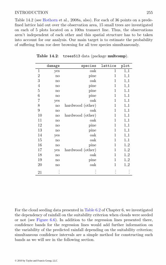
INTRODUCTION 255
Table 14.2 (see Hothorn et al., 2008a, also). For each of 36 points on a prede-fined lattice laid out over the observation area, 15 small trees are investigatedon each of 5 plots located on a 100m transect line. Thus, the observationsaren’t independent of each other and this spatial structure has to be takeninto account for our analysis. Our main target is to estimate the probabilityof suffering from roe deer browsing for all tree species simultaneously.
Table 14.2: trees513 data (package multcomp).
damage species lattice plot
1 yes oak 1 1 12 no pine 1 1 13 no oak 1 1 14 no pine 1 1 15 no pine 1 1 16 no pine 1 1 17 yes oak 1 1 18 no hardwood (other) 1 1 19 no oak 1 1 110 no hardwood (other) 1 1 111 no oak 1 1 112 no pine 1 1 113 no pine 1 1 114 yes oak 1 1 115 no oak 1 1 116 no pine 1 1 217 yes hardwood (other) 1 1 218 no oak 1 1 219 no pine 1 1 220 no oak 1 1 2
21...
......
...
For the cloud seeding data presented in Table 6.2 of Chapter 6, we investigatedthe dependency of rainfall on the suitability criterion when clouds were seededor not (see Figure 6.6). In addition to the regression lines presented there,confidence bands for the regression lines would add further information onthe variability of the predicted rainfall depending on the suitability criterion;simultaneous confidence intervals are a simple method for constructing suchbands as we will see in the following section.
© 2010 by Taylor and Francis Group, LLC

256 SIMULTANEOUS INFERENCE AND MULTIPLE COMPARISONS
14.2 Simultaneous Inference and Multiple Comparisons
Multiplicity is an intrinsic problem of any simultaneous inference. If each ofk, say, null hypotheses is tested at nominal level α on the same data set,the overall type I error rate can be substantially larger than α. That is, theprobability of at least one erroneous rejection is larger than α for k ≥ 2.Simultaneous inference procedures adjust for multiplicity and thus ensure thatthe overall type I error remains below the pre-specified significance level α.
The term multiple comparison procedure refers to simultaneous inference,i.e., simultaneous tests or confidence intervals, where the main interest is incomparing characteristics of different groups represented by a nominal factor.In fact, we have already seen such a procedure in Chapter 5 where multi-ple differences of mean rat weights were compared for all combinations ofthe mother rat’s genotype (Figure 5.5). Further examples of such multiplecomparison procedures include Dunnett’s many-to-one comparisons, sequen-tial pairwise contrasts, comparisons with the average, change-point analyses,dose-response contrasts, etc. These procedures are all well established for clas-sical regression and ANOVA models allowing for covariates and/or factorialtreatment structures with i.i.d. normal errors and constant variance. For ageneral reading on multiple comparison procedures we refer to Hochberg andTamhane (1987) and Hsu (1996).
Here, we follow a slightly more general approach allowing for null hypotheseson arbitrary model parameters, not only mean differences. Each individual nullhypothesis is specified through a linear combination of elemental model param-eters and we allow for k of such null hypotheses to be tested simultaneously,regardless of the number of elemental model parameters p. More precisely, weassume that our model contains fixed but unknown p-dimensional elementalparameters θ. We are primarily interested in linear functions ϑ := Kθ of theparameter vector θ as specified through the constant k × p matrix K. Forexample, in a linear model
yi = β0 + β1xi1 + · · · + βqxiq + εi
as introduced in Chapter 6, we might be interested in inference about theparameter β1, βq and β2 − β1. Chapter 6 offers methods for answering eachof these questions separately but does not provide an answer for all threequestions together. We can formulate the three inference problems as a linearcombination of the elemental parameter vector θ = (β0, β1, . . . , βq) as (herefor q = 3)
Kθ =
0 1 0 00 0 0 10 −1 1 0
θ = (β1, βq, β2 − β1)⊤ =: ϑ.
The global null hypothesis now reads
H0 : ϑ := Kθ = m,
where θ are the elemental model parameters that are estimated by some esti-
© 2010 by Taylor and Francis Group, LLC

ANALYSIS USING R 257
mate θ, K is the matrix defining linear functions of the elemental parametersresulting in our parameters of interest ϑ and m is a k-vector of constants. Thenull hypothesis states that ϑj = mj for all j = 1, . . . , k, where mj is somepredefined scalar being zero in most applications. The global hypothesis H0 isclassically tested using an F -test in linear and ANOVA models (see Chapter 5and Chapter 6). Such a test procedure gives only the answer ϑj 6= mj for atleast one j but doesn’t tell us which subset of our null hypotheses actuallycan be rejected. Here, we are mainly interested in which of the k partial hy-potheses H
j0 : ϑj = mj for j = 1, . . . , k are actually false. A simultaneous
inference procedure gives us information about which of these k hypothesescan be rejected in light of the data.
The estimated elemental parameters θ are normally distributed in classicallinear models and consequently, the estimated parameters of interest ϑ = Kθ
share this property. It can be shown that the t-statistics(
ϑ1 − m1
se(ϑ1), . . . ,
ϑk − mk
se(ϑk)
)
follow a joint multivariate k-dimensional t-distribution with correlation matrixCor. This correlation matrix and the standard deviations of our estimated pa-rameters of interest ϑj can be estimated from the data. In most other models,
the parameter estimates θ are only asymptotically normal distributed. In thissituation, the joint limiting distribution of all t-statistics on the parametersof interest is a k-variate normal distribution with zero mean and correlationmatrix Cor which can be estimated as well.
The key aspect of simultaneous inference procedures is to take these jointdistributions and thus the correlation among the estimated parameters ofinterest into account when constructing p-values and confidence intervals. Thedetailed technical aspects are computationally demanding since one has tocarefully evaluate multivariate distribution functions by means of numericalintegration procedures. However, these difficulties are rather unimportant tothe data analyst. For a detailed treatment of the statistical methodology werefer to Hothorn et al. (2008a).
14.3 Analysis Using R
14.3.1 Genetic Components of Alcoholism
We start with a graphical display of the data. Three parallel boxplots shownin Figure 14.1 indicate increasing expression levels of alpha synuclein mRNAfor longer NACP -REP1 alleles.
In order to model this relationship, we start fitting a simple one-way ANOVAmodel of the form yij = µ + γi + εij to the data with independent normalerrors εij ∼ N (0, σ2), j ∈ {short, intermediate, long}, and i = 1, . . . , nj . Theparameters µ + γshort, µ + γintermediate and µ + γlong can be interpreted asthe mean expression levels in the corresponding groups. As already discussed
© 2010 by Taylor and Francis Group, LLC

258 SIMULTANEOUS INFERENCE AND MULTIPLE COMPARISONS
R> n <- table(alpha$alength)
R> levels(alpha$alength) <- abbreviate(levels(alpha$alength), 4)
R> plot(elevel ~ alength, data = alpha, varwidth = TRUE,
+ ylab = "Expression Level",
+ xlab = "NACP-REP1 Allele Length")
R> axis(3, at = 1:3, labels = paste("n = ", n))
shrt intr long
−2
02
46
NACP−REP1 Allele Length
Exp
ressio
n L
eve
l
n = 24 n = 58 n = 15
Figure 14.1 Distribution of levels of expressed alpha synuclein mRNA in three
groups defined by the NACP-REP1 allele lengths.
in Chapter 5, this model description is overparameterised. A standard ap-proach is to consider a suitable re-parameterization. The so-called “treatmentcontrast” vector θ = (µ, γintermediate − γshort, γlong − γshort) (the default re-parameterization used as elemental parameters in R) is one possibility and isequivalent to imposing the restriction γshort = 0.
In addition, we define all comparisons among our three groups by choos-ing K such that Kθ contains all three group differences (Tukey’s all-pairwisecomparisons):
KTukey =
0 1 00 0 10 −1 1
with parameters of interest
ϑTukey = KTukeyθ = (γintermediate − γshort, γlong − γshort, γlong − γintermediate).
© 2010 by Taylor and Francis Group, LLC
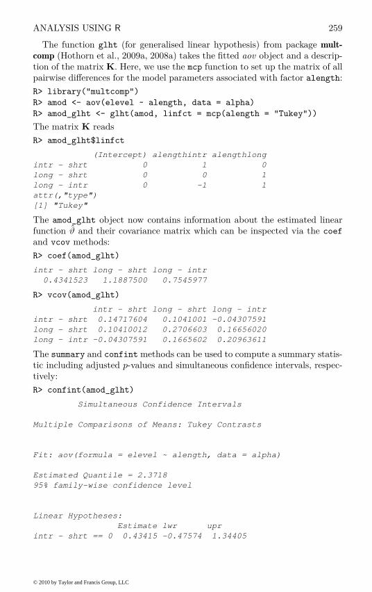
ANALYSIS USING R 259
The function glht (for generalised linear hypothesis) from package mult-
comp (Hothorn et al., 2009a, 2008a) takes the fitted aov object and a descrip-tion of the matrix K. Here, we use the mcp function to set up the matrix of allpairwise differences for the model parameters associated with factor alength:
R> library("multcomp")
R> amod <- aov(elevel ~ alength, data = alpha)
R> amod_glht <- glht(amod, linfct = mcp(alength = "Tukey"))
The matrix K reads
R> amod_glht$linfct
(Intercept) alengthintr alengthlong
intr - shrt 0 1 0
long - shrt 0 0 1
long - intr 0 -1 1
attr(,"type")
[1] "Tukey"
The amod_glht object now contains information about the estimated linearfunction ϑ and their covariance matrix which can be inspected via the coef
and vcov methods:
R> coef(amod_glht)
intr - shrt long - shrt long - intr
0.4341523 1.1887500 0.7545977
R> vcov(amod_glht)
intr - shrt long - shrt long - intr
intr - shrt 0.14717604 0.1041001 -0.04307591
long - shrt 0.10410012 0.2706603 0.16656020
long - intr -0.04307591 0.1665602 0.20963611
The summary and confint methods can be used to compute a summary statis-tic including adjusted p-values and simultaneous confidence intervals, respec-tively:
R> confint(amod_glht)
Simultaneous Confidence Intervals
Multiple Comparisons of Means: Tukey Contrasts
Fit: aov(formula = elevel ~ alength, data = alpha)
Estimated Quantile = 2.3718
95% family-wise confidence level
Linear Hypotheses:
Estimate lwr upr
intr - shrt == 0 0.43415 -0.47574 1.34405
© 2010 by Taylor and Francis Group, LLC
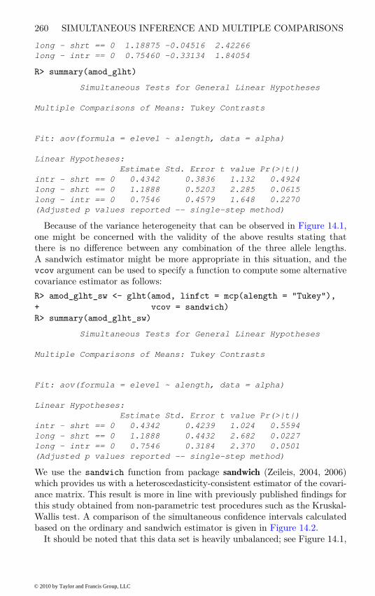
260 SIMULTANEOUS INFERENCE AND MULTIPLE COMPARISONS
long - shrt == 0 1.18875 -0.04516 2.42266
long - intr == 0 0.75460 -0.33134 1.84054
R> summary(amod_glht)
Simultaneous Tests for General Linear Hypotheses
Multiple Comparisons of Means: Tukey Contrasts
Fit: aov(formula = elevel ~ alength, data = alpha)
Linear Hypotheses:
Estimate Std. Error t value Pr(>|t|)
intr - shrt == 0 0.4342 0.3836 1.132 0.4924
long - shrt == 0 1.1888 0.5203 2.285 0.0615
long - intr == 0 0.7546 0.4579 1.648 0.2270
(Adjusted p values reported -- single-step method)
Because of the variance heterogeneity that can be observed in Figure 14.1,one might be concerned with the validity of the above results stating thatthere is no difference between any combination of the three allele lengths.A sandwich estimator might be more appropriate in this situation, and thevcov argument can be used to specify a function to compute some alternativecovariance estimator as follows:
R> amod_glht_sw <- glht(amod, linfct = mcp(alength = "Tukey"),
+ vcov = sandwich)
R> summary(amod_glht_sw)
Simultaneous Tests for General Linear Hypotheses
Multiple Comparisons of Means: Tukey Contrasts
Fit: aov(formula = elevel ~ alength, data = alpha)
Linear Hypotheses:
Estimate Std. Error t value Pr(>|t|)
intr - shrt == 0 0.4342 0.4239 1.024 0.5594
long - shrt == 0 1.1888 0.4432 2.682 0.0227
long - intr == 0 0.7546 0.3184 2.370 0.0501
(Adjusted p values reported -- single-step method)
We use the sandwich function from package sandwich (Zeileis, 2004, 2006)which provides us with a heteroscedasticity-consistent estimator of the covari-ance matrix. This result is more in line with previously published findings forthis study obtained from non-parametric test procedures such as the Kruskal-Wallis test. A comparison of the simultaneous confidence intervals calculatedbased on the ordinary and sandwich estimator is given in Figure 14.2.
It should be noted that this data set is heavily unbalanced; see Figure 14.1,
© 2010 by Taylor and Francis Group, LLC
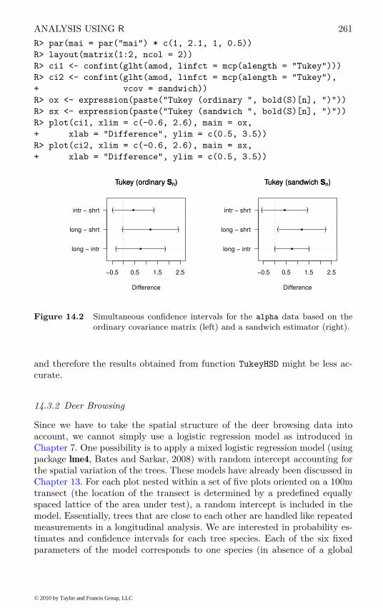
ANALYSIS USING R 261
R> par(mai = par("mai") * c(1, 2.1, 1, 0.5))
R> layout(matrix(1:2, ncol = 2))
R> ci1 <- confint(glht(amod, linfct = mcp(alength = "Tukey")))
R> ci2 <- confint(glht(amod, linfct = mcp(alength = "Tukey"),
+ vcov = sandwich))
R> ox <- expression(paste("Tukey (ordinary ", bold(S)[n], ")"))
R> sx <- expression(paste("Tukey (sandwich ", bold(S)[n], ")"))
R> plot(ci1, xlim = c(-0.6, 2.6), main = ox,
+ xlab = "Difference", ylim = c(0.5, 3.5))
R> plot(ci2, xlim = c(-0.6, 2.6), main = sx,
+ xlab = "Difference", ylim = c(0.5, 3.5))
Tukey (ordinary Sn)
−0.5 0.5 1.5 2.5
long − intr
long − shrt
intr − shrt (
(
(
)
)
)
l
l
l
Tukey (ordinary Sn)
Difference
Tukey (sandwich Sn)
−0.5 0.5 1.5 2.5
long − intr
long − shrt
intr − shrt (
(
(
)
)
)
l
l
l
Tukey (sandwich Sn)
Difference
Figure 14.2 Simultaneous confidence intervals for the alpha data based on the
ordinary covariance matrix (left) and a sandwich estimator (right).
and therefore the results obtained from function TukeyHSD might be less ac-curate.
14.3.2 Deer Browsing
Since we have to take the spatial structure of the deer browsing data intoaccount, we cannot simply use a logistic regression model as introduced inChapter 7. One possibility is to apply a mixed logistic regression model (usingpackage lme4, Bates and Sarkar, 2008) with random intercept accounting forthe spatial variation of the trees. These models have already been discussed inChapter 13. For each plot nested within a set of five plots oriented on a 100mtransect (the location of the transect is determined by a predefined equallyspaced lattice of the area under test), a random intercept is included in themodel. Essentially, trees that are close to each other are handled like repeatedmeasurements in a longitudinal analysis. We are interested in probability es-timates and confidence intervals for each tree species. Each of the six fixedparameters of the model corresponds to one species (in absence of a global
© 2010 by Taylor and Francis Group, LLC
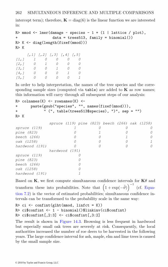
262 SIMULTANEOUS INFERENCE AND MULTIPLE COMPARISONS
intercept term); therefore, K = diag(6) is the linear function we are interestedin:
R> mmod <- lmer(damage ~ species - 1 + (1 | lattice / plot),
+ data = trees513, family = binomial())
R> K <- diag(length(fixef(mmod)))
R> K
[,1] [,2] [,3] [,4] [,5]
[1,] 1 0 0 0 0
[2,] 0 1 0 0 0
[3,] 0 0 1 0 0
[4,] 0 0 0 1 0
[5,] 0 0 0 0 1
In order to help interpretation, the names of the tree species and the corre-sponding sample sizes (computed via table) are added to K as row names;this information will carry through all subsequent steps of our analysis:
R> colnames(K) <- rownames(K) <-
+ paste(gsub("species", "", names(fixef(mmod))),
+ " (", table(trees513$species), ")", sep = "")
R> K
spruce (119) pine (823) beech (266) oak (1258)
spruce (119) 1 0 0 0
pine (823) 0 1 0 0
beech (266) 0 0 1 0
oak (1258) 0 0 0 1
hardwood (191) 0 0 0 0
hardwood (191)
spruce (119) 0
pine (823) 0
beech (266) 0
oak (1258) 0
hardwood (191) 1
Based on K, we first compute simultaneous confidence intervals for Kθ and
transform these into probabilities. Note that(
1 + exp(−ϑ))
−1
(cf. Equa-
tion 7.2) is the vector of estimated probabilities; simultaneous confidence in-tervals can be transformed to the probability scale in the same way:
R> ci <- confint(glht(mmod, linfct = K))
R> ci$confint <- 1 - binomial()$linkinv(ci$confint)
R> ci$confint[,2:3] <- ci$confint[,3:2]
The result is shown in Figure 14.3. Browsing is less frequent in hardwoodbut especially small oak trees are severely at risk. Consequently, the localauthorities increased the number of roe deers to be harvested in the followingyears. The large confidence interval for ash, maple, elm and lime trees is causedby the small sample size.
© 2010 by Taylor and Francis Group, LLC
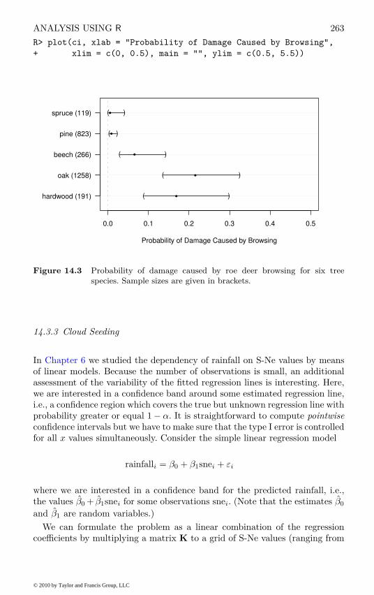
ANALYSIS USING R 263
R> plot(ci, xlab = "Probability of Damage Caused by Browsing",
+ xlim = c(0, 0.5), main = "", ylim = c(0.5, 5.5))
0.0 0.1 0.2 0.3 0.4 0.5
hardwood (191)
oak (1258)
beech (266)
pine (823)
spruce (119) (
(
(
(
(
)
)
)
)
)
l
l
l
l
l
Probability of Damage Caused by Browsing
Figure 14.3 Probability of damage caused by roe deer browsing for six tree
species. Sample sizes are given in brackets.
14.3.3 Cloud Seeding
In Chapter 6 we studied the dependency of rainfall on S-Ne values by meansof linear models. Because the number of observations is small, an additionalassessment of the variability of the fitted regression lines is interesting. Here,we are interested in a confidence band around some estimated regression line,i.e., a confidence region which covers the true but unknown regression line withprobability greater or equal 1 − α. It is straightforward to compute pointwise
confidence intervals but we have to make sure that the type I error is controlledfor all x values simultaneously. Consider the simple linear regression model
rainfalli = β0 + β1snei + εi
where we are interested in a confidence band for the predicted rainfall, i.e.,the values β0 + β1snei for some observations snei. (Note that the estimates β0
and β1 are random variables.)
We can formulate the problem as a linear combination of the regressioncoefficients by multiplying a matrix K to a grid of S-Ne values (ranging from
© 2010 by Taylor and Francis Group, LLC
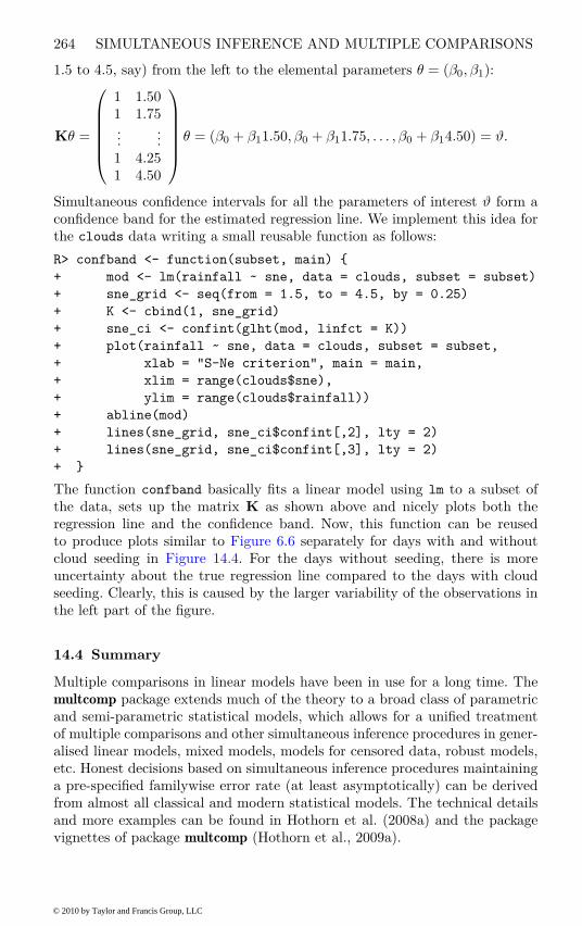
264 SIMULTANEOUS INFERENCE AND MULTIPLE COMPARISONS
1.5 to 4.5, say) from the left to the elemental parameters θ = (β0, β1):
Kθ =
1 1.501 1.75...
...1 4.251 4.50
θ = (β0 + β11.50, β0 + β11.75, . . . , β0 + β14.50) = ϑ.
Simultaneous confidence intervals for all the parameters of interest ϑ form aconfidence band for the estimated regression line. We implement this idea forthe clouds data writing a small reusable function as follows:
R> confband <- function(subset, main) {
+ mod <- lm(rainfall ~ sne, data = clouds, subset = subset)
+ sne_grid <- seq(from = 1.5, to = 4.5, by = 0.25)
+ K <- cbind(1, sne_grid)
+ sne_ci <- confint(glht(mod, linfct = K))
+ plot(rainfall ~ sne, data = clouds, subset = subset,
+ xlab = "S-Ne criterion", main = main,
+ xlim = range(clouds$sne),
+ ylim = range(clouds$rainfall))
+ abline(mod)
+ lines(sne_grid, sne_ci$confint[,2], lty = 2)
+ lines(sne_grid, sne_ci$confint[,3], lty = 2)
+ }
The function confband basically fits a linear model using lm to a subset ofthe data, sets up the matrix K as shown above and nicely plots both theregression line and the confidence band. Now, this function can be reusedto produce plots similar to Figure 6.6 separately for days with and withoutcloud seeding in Figure 14.4. For the days without seeding, there is moreuncertainty about the true regression line compared to the days with cloudseeding. Clearly, this is caused by the larger variability of the observations inthe left part of the figure.
14.4 Summary
Multiple comparisons in linear models have been in use for a long time. Themultcomp package extends much of the theory to a broad class of parametricand semi-parametric statistical models, which allows for a unified treatmentof multiple comparisons and other simultaneous inference procedures in gener-alised linear models, mixed models, models for censored data, robust models,etc. Honest decisions based on simultaneous inference procedures maintaininga pre-specified familywise error rate (at least asymptotically) can be derivedfrom almost all classical and modern statistical models. The technical detailsand more examples can be found in Hothorn et al. (2008a) and the packagevignettes of package multcomp (Hothorn et al., 2009a).
© 2010 by Taylor and Francis Group, LLC

SUMMARY 265
R> layout(matrix(1:2, ncol = 2))
R> confband(clouds$seeding == "no", main = "No seeding")
R> confband(clouds$seeding == "yes", main = "Seeding")
1.5 2.5 3.5 4.5
02
46
81
0
No seeding
S−Ne criterion
rain
fall
1.5 2.5 3.5 4.5
02
46
81
0
Seeding
S−Ne criterion
rain
fall
Figure 14.4 Regression relationship between S-Ne criterion and rainfall with and
without seeding. The confidence bands cover the area within the
dashed curves.
Exercises
Ex. 14.1 Compare the results of glht and TukeyHSD on the alpha data.
Ex. 14.2 Consider the linear model fitted to the clouds data as summarisedin Figure 6.5. Set up a matrix K corresponding to the global null hypoth-esis that all interaction terms present in the model are zero. Test both theglobal hypothesis and all hypotheses corresponding to each of the inter-action terms. Which interaction remains significant after adjustment formultiple testing?
Ex. 14.3 For the logistic regression model presented in Figure 7.7 performa multiplicity adjusted test on all regression coefficients (except for theintercept) being zero. Do the conclusions drawn in Chapter 7 remain valid?
© 2010 by Taylor and Francis Group, LLC

CHAPTER 15
Meta-Analysis: Nicotine Gum andSmoking Cessation and the Efficacy of
BCG Vaccine in the Treatment ofTuberculosis
15.1 Introduction
Cigarette smoking is the leading cause of preventable death in the UnitedStates and kills more Americans than AIDS, alcohol, illegal drug use, caraccidents, fires, murders and suicides combined. It has been estimated that430,000 Americans die from smoking every year. Fighting tobacco use is, con-sequently, one of the major public health goals of our time and there are nowmany programs available designed to help smokers quit. One of the major aidsused in these programs is nicotine chewing gum, which acts as a substituteoral activity and provides a source of nicotine that reduces the withdrawalsymptoms experienced when smoking is stopped. But separate randomisedclinical trials of nicotine gum have been largely inconclusive, leading Silagy(2003) to consider combining the results from 26 such studies found from anextensive literature search. The results of these trials in terms of numbers ofpeople in the treatment arm and the control arm who stopped smoking for atleast 6 months after treatment are given in Table 15.1.
Bacille Calmette Guerin (BCG) is the most widely used vaccination in theworld. Developed in the 1930s and made of a live, weakened strain of Mycobac-terium bovis, the BCG is the only vaccination available against tuberculosis(TBC) today. Colditz et al. (1994) report data from 13 clinical trials of BCGvaccine each investigating its efficacy in the prevention of tuberculosis. Thenumber of subjects suffering from TB with or without BCG vaccination aregiven in Table 15.2. In addition, the table contains the values of two othervariables for each study, namely, the geographic latitude of the place wherethe study was undertaken and the year of publication. These two variableswill be used to investigate and perhaps explain any heterogeneity among thestudies.
267
© 2010 by Taylor and Francis Group, LLC
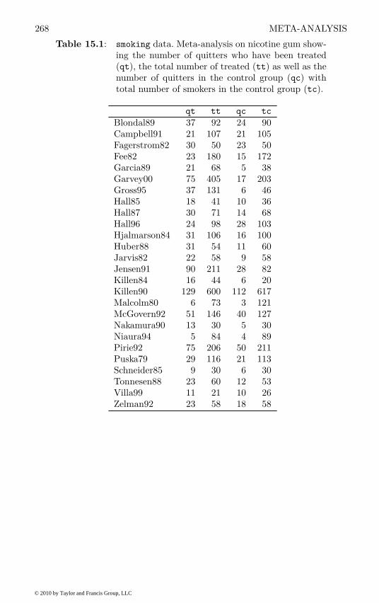
268 META-ANALYSIS
Table 15.1: smoking data. Meta-analysis on nicotine gum show-ing the number of quitters who have been treated(qt), the total number of treated (tt) as well as thenumber of quitters in the control group (qc) withtotal number of smokers in the control group (tc).
qt tt qc tc
Blondal89 37 92 24 90Campbell91 21 107 21 105Fagerstrom82 30 50 23 50Fee82 23 180 15 172Garcia89 21 68 5 38Garvey00 75 405 17 203Gross95 37 131 6 46Hall85 18 41 10 36Hall87 30 71 14 68Hall96 24 98 28 103Hjalmarson84 31 106 16 100Huber88 31 54 11 60Jarvis82 22 58 9 58Jensen91 90 211 28 82Killen84 16 44 6 20Killen90 129 600 112 617Malcolm80 6 73 3 121McGovern92 51 146 40 127Nakamura90 13 30 5 30Niaura94 5 84 4 89Pirie92 75 206 50 211Puska79 29 116 21 113Schneider85 9 30 6 30Tonnesen88 23 60 12 53Villa99 11 21 10 26Zelman92 23 58 18 58
© 2010 by Taylor and Francis Group, LLC
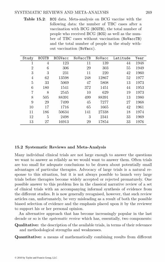
SYSTEMATIC REVIEWS AND META-ANALYSIS 269
Table 15.2: BCG data. Meta-analysis on BCG vaccine with thefollowing data: the number of TBC cases after avaccination with BCG (BCGTB), the total number ofpeople who received BCG (BCG) as well as the num-ber of TBC cases without vaccination (NoVaccTB)and the total number of people in the study with-out vaccination (NoVacc).
Study BCGTB BCGVacc NoVaccTB NoVacc Latitude Year
1 4 123 11 139 44 19482 6 306 29 303 55 19493 3 231 11 220 42 19604 62 13598 248 12867 52 19775 33 5069 47 5808 13 19736 180 1541 372 1451 44 19537 8 2545 10 629 19 19738 505 88391 499 88391 13 19809 29 7499 45 7277 27 1968
10 17 1716 65 1665 42 196111 186 50634 141 27338 18 197412 5 2498 3 2341 33 196913 27 16913 29 17854 33 1976
15.2 Systematic Reviews and Meta-Analysis
Many individual clinical trials are not large enough to answer the questionswe want to answer as reliably as we would want to answer them. Often trialsare too small for adequate conclusions to be drawn about potentially smalladvantages of particular therapies. Advocacy of large trials is a natural re-sponse to this situation, but it is not always possible to launch very largetrials before therapies become widely accepted or rejected prematurely. Onepossible answer to this problem lies in the classical narrative review of a setof clinical trials with an accompanying informal synthesis of evidence fromthe different studies. It is now generally recognised, however, that such reviewarticles can, unfortunately, be very misleading as a result of both the possiblebiased selection of evidence and the emphasis placed upon it by the reviewerto support his or her personal opinion.
An alternative approach that has become increasingly popular in the lastdecade or so is the systematic review which has, essentially, two components:
Qualitative: the description of the available trials, in terms of their relevanceand methodological strengths and weaknesses.
Quantitative: a means of mathematically combining results from different
© 2010 by Taylor and Francis Group, LLC

270 META-ANALYSIS
studies, even when these studies have used different measures to assess thedependent variable.
The quantitative component of a systematic review is usually known as ameta-analysis, defined in the Cambridge Dictionary of Statistics in the Medical
Sciences (Everitt, 2002a), as follows:
A collection of techniques whereby the results of two or more independent stud-ies are statistically combined to yield an overall answer to a question of interest.The rationale behind this approach is to provide a test with more power than isprovided by the separate studies themselves. The procedure has become increas-ingly popular in the last decade or so, but is not without its critics, particularlybecause of the difficulties of knowing which studies should be included and towhich population final results actually apply.
It is now generally accepted that meta-analysis gives the systematic reviewan objectivity that is inevitably lacking in literature reviews and can alsohelp the process to achieve greater precision and generalisability of findingsthan any single study. Chalmers and Lau (1993) make the point that both theclassical review article and a meta-analysis can be biased, but that at leastthe writer of a meta-analytic paper is required by the rudimentary standardsof the discipline to give the data on which any conclusions are based, andto defend the development of these conclusions by giving evidence that allavailable data are included, or to give the reasons for not including the data.Chalmers and Lau (1993) conclude
It seems obvious that a discipline that requires all available data be revealedand included in an analysis has an advantage over one that has traditionally notpresented analyses of all the data in which conclusions are based.
The demand for systematic reviews of health care interventions has devel-oped rapidly during the last decade, initiated by the widespread adoption ofthe principles of evidence-based medicine amongst both health care practition-ers and policy makers. Such reviews are now increasingly used as a basis forboth individual treatment decisions and the funding of health care and healthcare research worldwide. Systematic reviews have a number of aims:
• To review systematically the available evidence from a particular researcharea,
• To provide quantitative summaries of the results from each study,
• To combine the results across studies if appropriate; such combination ofresults typically leads to greater statistical power in estimating treatmenteffects,
• To assess the amount of variability between studies,
• To estimate the degree of benefit associated with a particular study treat-ment,
• To identify study characteristics associated with particularly effective treat-ments.
Perhaps the most important aspect of a meta-analysis is study selection.
© 2010 by Taylor and Francis Group, LLC

STATISTICS OF META-ANALYSIS 271
Selection is a matter of inclusion and exclusion and the judgements requiredare, at times, problematic. But we shall say nothing about this fundamentalcomponent of a meta-analysis here since it has been comprehensively dealtwith by a number of authors, including Chalmers and Lau (1993) and Petitti(2000). Instead we shall concentrate on the statistics of meta-analysis.
15.3 Statistics of Meta-Analysis
Two models that are frequently used in the meta-analysis of medical studiesare the fixed effects and random effects models. Whilst the former assumesthat each observed individual study result is estimating a common unknownoverall pooled effect, the latter assumes that each individual observed resultis estimating its own unknown underlying effect, which in turn is estimating acommon population mean. Thus the random effects model specifically allowsfor the existence of between-study heterogeneity as well as within-study vari-
ability. DeMets (1987) and Bailey (1987) discuss the strengths and weaknessesof the two competing models. Bailey suggests that when the research questioninvolves extrapolation to the future – will the treatment have an effect, onthe average – then the random effects model for the studies is the appropriateone. The research question implicitly assumes that there is a population ofstudies from which those analysed in the meta-analysis were sampled, and an-ticipate future studies being conducted or previously unknown studies beinguncovered.
When the research question concerns whether treatment has produced aneffect, on the average, in the set of studies being analysed, then the fixed effectsmodel for the studies may be the appropriate one; here there is no interest ingeneralising the results to other studies.
Many statisticians believe that random effects models are more appropriatethan fixed effects models for meta-analysis because between-study variationis an important source of uncertainty that should not be ignored.
15.3.1 Fixed Effects Model – Mantel-Haenszel
This model uses as its estimate of the common pooled effect, Y , a weightedaverage of the individual study effects, the weights being inversely proportionalto the within-study variances. Specifically
Y =
k∑
i=1
WiYi
k∑
i=1
Wi
(15.1)
where k is the number of the studies in the meta-analysis, Yi is the effect sizeestimated in the ith study (this might be a odds-ratio, log-odds ratio, relativerisk or difference in means, for example), and Wi = 1/Vi where Vi is the withinstudy estimate of variance for the ith study. The estimated variance of Y is
© 2010 by Taylor and Francis Group, LLC
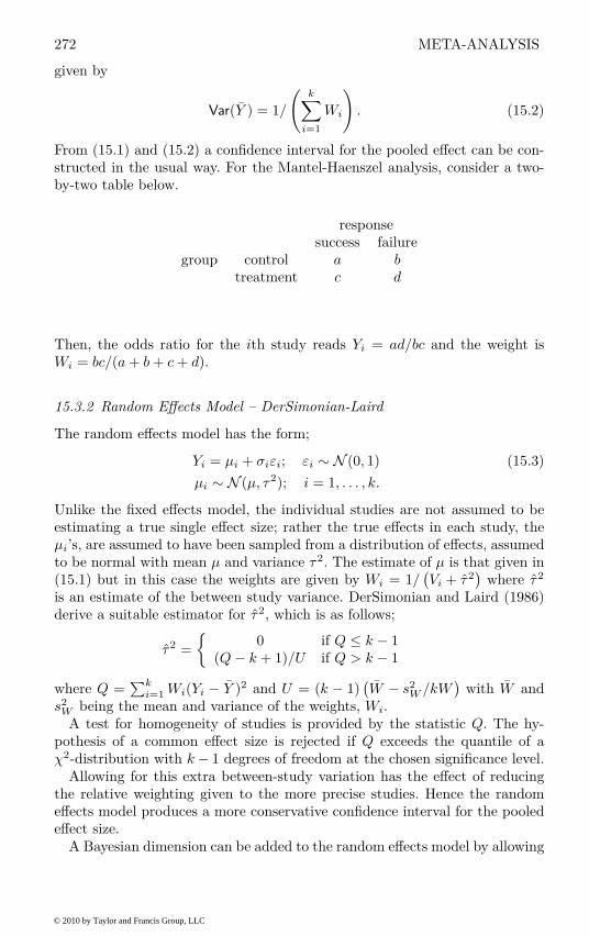
272 META-ANALYSIS
given by
Var(Y ) = 1/
(
k∑
i=1
Wi
)
. (15.2)
From (15.1) and (15.2) a confidence interval for the pooled effect can be con-structed in the usual way. For the Mantel-Haenszel analysis, consider a two-by-two table below.
responsesuccess failure
group control a b
treatment c d
Then, the odds ratio for the ith study reads Yi = ad/bc and the weight isWi = bc/(a + b + c + d).
15.3.2 Random Effects Model – DerSimonian-Laird
The random effects model has the form;
Yi = µi + σiεi; εi ∼ N (0, 1) (15.3)
µi ∼ N (µ, τ2); i = 1, . . . , k.
Unlike the fixed effects model, the individual studies are not assumed to beestimating a true single effect size; rather the true effects in each study, theµi’s, are assumed to have been sampled from a distribution of effects, assumedto be normal with mean µ and variance τ
2. The estimate of µ is that given in(15.1) but in this case the weights are given by Wi = 1/
(
Vi + τ2)
where τ2
is an estimate of the between study variance. DerSimonian and Laird (1986)derive a suitable estimator for τ
2, which is as follows;
τ2 =
{
0 if Q ≤ k − 1(Q − k + 1)/U if Q > k − 1
where Q =∑k
i=1Wi(Yi − Y )2 and U = (k − 1)
(
W − s2
W /kW
)
with W ands
2
W being the mean and variance of the weights, Wi.A test for homogeneity of studies is provided by the statistic Q. The hy-
pothesis of a common effect size is rejected if Q exceeds the quantile of aχ
2-distribution with k − 1 degrees of freedom at the chosen significance level.Allowing for this extra between-study variation has the effect of reducing
the relative weighting given to the more precise studies. Hence the randomeffects model produces a more conservative confidence interval for the pooledeffect size.
A Bayesian dimension can be added to the random effects model by allowing
© 2010 by Taylor and Francis Group, LLC
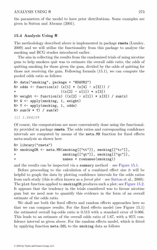
ANALYSIS USING R 273
the parameters of the model to have prior distributions. Some examples aregiven in Sutton and Abrams (2001).
15.4 Analysis Using R
The methodology described above is implemented in package rmeta (Lumley,2009) and we will utilise the functionality from this package to analyse thesmoking and BCG studies introduced earlier.
The aim in collecting the results from the randomised trials of using nicotinegum to help smokers quit was to estimate the overall odds ratio, the odds ofquitting smoking for those given the gum, divided by the odds of quitting forthose not receiving the gum. Following formula (15.1), we can compute thepooled odds ratio as follows:
R> data("smoking", package = "HSAUR2")
R> odds <- function(x) (x[1] * (x[4] - x[3])) /
+ ((x[2] - x[1]) * x[3])
R> weight <- function(x) ((x[2] - x[1]) * x[3]) / sum(x)
R> W <- apply(smoking, 1, weight)
R> Y <- apply(smoking, 1, odds)
R> sum(W * Y) / sum(W)
[1] 1.664159
Of course, the computations are more conveniently done using the functional-ity provided in package rmeta. The odds ratios and corresponding confidenceintervals are computed by means of the meta.MH function for fixed effectsmeta-analysis as shown here
R> library("rmeta")
R> smokingOR <- meta.MH(smoking[["tt"]], smoking[["tc"]],
+ smoking[["qt"]], smoking[["qc"]],
+ names = rownames(smoking))
and the results can be inspected via a summary method – see Figure 15.1.Before proceeding to the calculation of a combined effect size it will be
helpful to graph the data by plotting confidence intervals for the odds ratiosfrom each study (this is often known as a forest plot – see Sutton et al., 2000).The plot function applied to smokingOR produces such a plot; see Figure 15.2.It appears that the tendency in the trials considered was to favour nicotinegum but we need now to quantify this evidence in the form of an overallestimate of the odds ratio.
We shall use both the fixed effects and random effects approaches here sothat we can compare results. For the fixed effects model (see Figure 15.1)the estimated overall log-odds ratio is 0.513 with a standard error of 0.066.This leads to an estimate of the overall odds ratio of 1.67, with a 95% con-fidence interval as given above. For the random effects model, which is fittedby applying function meta.DSL to the smoking data as follows
© 2010 by Taylor and Francis Group, LLC
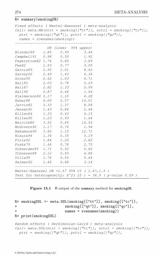
274 META-ANALYSIS
R> summary(smokingOR)
Fixed effects ( Mantel-Haenszel ) meta-analysis
Call: meta.MH(ntrt = smoking[["tt"]], nctrl = smoking[["tc"]],
ptrt = smoking[["qt"]], pctrl = smoking[["qc"]],
names = rownames(smoking))
------------------------------------
OR (lower 95% upper)
Blondal89 1.85 0.99 3.46
Campbell91 0.98 0.50 1.92
Fagerstrom82 1.76 0.80 3.89
Fee82 1.53 0.77 3.05
Garcia89 2.95 1.01 8.62
Garvey00 2.49 1.43 4.34
Gross95 2.62 1.03 6.71
Hall85 2.03 0.78 5.29
Hall87 2.82 1.33 5.99
Hall96 0.87 0.46 1.64
Hjalmarson84 2.17 1.10 4.28
Huber88 6.00 2.57 14.01
Jarvis82 3.33 1.37 8.08
Jensen91 1.43 0.84 2.44
Killen84 1.33 0.43 4.15
Killen90 1.23 0.93 1.64
Malcolm80 3.52 0.85 14.54
McGovern92 1.17 0.70 1.94
Nakamura90 3.82 1.15 12.71
Niaura94 1.34 0.35 5.19
Pirie92 1.84 1.20 2.82
Puska79 1.46 0.78 2.75
Schneider85 1.71 0.52 5.62
Tonnesen88 2.12 0.93 4.86
Villa99 1.76 0.55 5.64
Zelman92 1.46 0.68 3.14
------------------------------------
Mantel-Haenszel OR =1.67 95% CI ( 1.47,1.9 )
Test for heterogeneity: X^2( 25 ) = 34.9 ( p-value 0.09 )
Figure 15.1 R output of the summary method for smokingOR.
R> smokingDSL <- meta.DSL(smoking[["tt"]], smoking[["tc"]],
+ smoking[["qt"]], smoking[["qc"]],
+ names = rownames(smoking))
R> print(smokingDSL)
Random effects ( DerSimonian-Laird ) meta-analysis
Call: meta.DSL(ntrt = smoking[["tt"]], nctrl = smoking[["tc"]],
ptrt = smoking[["qt"]], pctrl = smoking[["qc"]],
© 2010 by Taylor and Francis Group, LLC

ANALYSIS USING R 275
R> plot(smokingOR, ylab = "")
Odds Ratio
0.40 1.00 2.51 6.31 15.85
Blondal89Campbell91Fagerstrom82Fee82Garcia89Garvey00Gross95Hall85Hall87Hall96Hjalmarson84Huber88Jarvis82Jensen91Killen84Killen90Malcolm80McGovern92Nakamura90Niaura94Pirie92Puska79Schneider85Tonnesen88Villa99Zelman92
Summary
Figure 15.2 Forest plot of observed effect sizes and 95% confidence intervals forthe nicotine gum studies.
© 2010 by Taylor and Francis Group, LLC

276 META-ANALYSIS
names = rownames(smoking))
Summary OR= 1.75 95% CI ( 1.48, 2.07 )
Estimated random effects variance: 0.05
the corresponding estimate is 1.751. Both models suggest that there is clearevidence that nicotine gum increases the odds of quitting. The random effectsconfidence interval is considerably wider than that from the fixed effects model;here the test of homogeneity of the studies is not significant implying that wemight use the fixed effects results. But the test is not particularly powerfuland it is more sensible to assume a priori that heterogeneity is present and sowe use the results from the random effects model.
15.5 Meta-Regression
The examination of heterogeneity of the effect sizes from the studies in ameta-analysis begins with the formal test for its presence, although in mostmeta-analyses such heterogeneity can almost be assumed to be present. Therewill be many possible sources of such heterogeneity and estimating how thesevarious factors affect the observed effect sizes in the studies chosen is oftenof considerable interest and importance, indeed usually more important thanthe relatively simplistic use of meta-analysis to determine a single summaryestimate of overall effect size. We can illustrate the process using the BCGvaccine data. We first find the estimate of the overall effect size from applyingthe fixed effects and the random effects models described previously:
R> data("BCG", package = "HSAUR2")
R> BCG_OR <- meta.MH(BCG[["BCGVacc"]], BCG[["NoVacc"]],
+ BCG[["BCGTB"]], BCG[["NoVaccTB"]],
+ names = BCG$Study)
R> BCG_DSL <- meta.DSL(BCG[["BCGVacc"]], BCG[["NoVacc"]],
+ BCG[["BCGTB"]], BCG[["NoVaccTB"]],
+ names = BCG$Study)
The results are inspected using the summary method as shown in Figures 15.3and 15.4.
For these data the test statistics for heterogeneity takes the value 163.16which, with 12 degrees of freedom, is highly significant; there is strong evi-dence of heterogeneity in the 13 studies. Applying the random effects modelto the data gives (see Figure 15.4) an estimated odds ratio 0.474, with a 95%confidence interval of (0.325, 0.69) and an estimated between-study varianceof 0.366.
To assess how the two covariates, latitude and year, relate to the observedeffect sizes we shall use multiple linear regression but will weight each ob-servation by Wi = (σ2 + V
2i )−1
, i = 1, . . . , 13, where σ2 is the estimated
between-study variance and V2i is the estimated variance from the ith study.
The required R code to fit the linear model via weighted least squares is:
R> studyweights <- 1 / (BCG_DSL$tau2 + BCG_DSL$selogs^2)
R> y <- BCG_DSL$logs
© 2010 by Taylor and Francis Group, LLC

PUBLICATION BIAS 277
R> summary(BCG_OR)
Fixed effects ( Mantel-Haenszel ) meta-analysis
Call: meta.MH(ntrt = BCG[["BCGVacc"]], nctrl = BCG[["NoVacc"]],
ptrt = BCG[["BCGTB"]], pctrl = BCG[["NoVaccTB"]],
names = BCG$Study)
------------------------------------
OR (lower 95% upper)
1 0.39 0.12 1.26
2 0.19 0.08 0.46
3 0.25 0.07 0.91
4 0.23 0.18 0.31
5 0.80 0.51 1.26
6 0.38 0.32 0.47
7 0.20 0.08 0.50
8 1.01 0.89 1.15
9 0.62 0.39 1.00
10 0.25 0.14 0.42
11 0.71 0.57 0.89
12 1.56 0.37 6.55
13 0.98 0.58 1.66
------------------------------------
Mantel-Haenszel OR =0.62 95% CI ( 0.57,0.68 )
Test for heterogeneity: X^2( 12 ) = 163.94 ( p-value 0 )
Figure 15.3 R output of the summary method for BCG_OR.
R> BCG_mod <- lm(y ~ Latitude + Year, data = BCG,
+ weights = studyweights)
and the results of the summary method are shown in Figure 15.5. There issome evidence that latitude is associated with observed effect size, the log-odds ratio becoming increasingly negative as latitude increases, as we can seefrom a scatterplot of the two variables with the added weighted regression fitseen in Figure 15.6.
15.6 Publication Bias
The selection of studies to be integrated by a meta-analysis will clearly havea bearing on the conclusions reached. Selection is a matter of inclusion andexclusion and the judgements required are often difficult; Chalmers and Lau(1993) discuss the general issues involved, but here we shall concentrate on theparticular potential problem of publication bias, which is a major problem,perhaps the major problem in meta-analysis.
Ensuring that a meta-analysis is truly representative can be problematic.It has long been known that journal articles are not a representative sampleof work addressed to any particular area of research (see Sterlin, 1959, Green-
© 2010 by Taylor and Francis Group, LLC

278 META-ANALYSIS
R> summary(BCG_DSL)
Random effects ( DerSimonian-Laird ) meta-analysis
Call: meta.DSL(ntrt = BCG[["BCGVacc"]], nctrl = BCG[["NoVacc"]],
ptrt = BCG[["BCGTB"]], pctrl = BCG[["NoVaccTB"]],
names = BCG$Study)
------------------------------------
OR (lower 95% upper)
1 0.39 0.12 1.26
2 0.19 0.08 0.46
3 0.25 0.07 0.91
4 0.23 0.18 0.31
5 0.80 0.51 1.26
6 0.38 0.32 0.47
7 0.20 0.08 0.50
8 1.01 0.89 1.15
9 0.62 0.39 1.00
10 0.25 0.14 0.42
11 0.71 0.57 0.89
12 1.56 0.37 6.55
13 0.98 0.58 1.66
------------------------------------
SummaryOR= 0.47 95% CI ( 0.32,0.69 )
Test for heterogeneity: X^2( 12 ) = 163.16 ( p-value 0 )
Estimated random effects variance: 0.37
Figure 15.4 R output of the summary method for BCG_DSL.
wald, 1975, Smith, 1980, for example). Research with statistically significantresults is potentially more likely to be submitted and published than workwith null or non-significant results (Easterbrook et al., 1991). The problemis made worse by the fact that many medical studies look at multiple out-comes, and there is a tendency for only those suggesting a significant effect tobe mentioned when the study is written up. Outcomes which show no cleartreatment effect are often ignored, and so will not be included in any later re-view of studies looking at those particular outcomes. Publication bias is likelyto lead to an over-representation of positive results.
Clearly then it becomes of some importance to assess the likelihood of publi-cation bias in any meta-analysis. A well-known, informal method of assessingpublication bias is the so-called funnel plot. This assumes that the resultsfrom smaller studies will be more widely spread around the mean effect be-cause of larger random error; a plot of a measure of the precision (such asinverse standard error or sample size) of the studies versus treatment effectfrom individual studies in a meta-analysis, should therefore be shaped like afunnel if there is no publication bias. If the chance of publication is greater
© 2010 by Taylor and Francis Group, LLC
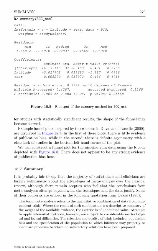
SUMMARY 279
R> summary(BCG_mod)
Call:
lm(formula = y ~ Latitude + Year, data = BCG,
weights = studyweights)
Residuals:
Min 1Q Median 3Q Max
-1.66012 -0.36910 -0.02937 0.31565 1.26040
Coefficients:
Estimate Std. Error t value Pr(>|t|)
(Intercept) -16.199115 37.605403 -0.431 0.6758
Latitude -0.025808 0.013680 -1.887 0.0886
Year 0.008279 0.018972 0.436 0.6718
Residual standard error: 0.7992 on 10 degrees of freedom
Multiple R-squared: 0.4387, Adjusted R-squared: 0.3265
F-statistic: 3.909 on 2 and 10 DF, p-value: 0.05569
Figure 15.5 R output of the summary method for BCG_mod.
for studies with statistically significant results, the shape of the funnel maybecome skewed.
Example funnel plots, inspired by those shown in Duval and Tweedie (2000),are displayed in Figure 15.7. In the first of these plots, there is little evidenceof publication bias, while in the second, there is definite asymmetry with aclear lack of studies in the bottom left hand corner of the plot.
We can construct a funnel plot for the nicotine gum data using the R codedepicted with Figure 15.8. There does not appear to be any strong evidenceof publication bias here.
15.7 Summary
It is probably fair to say that the majority of statisticians and clinicians arelargely enthusiastic about the advantages of meta-analysis over the classicalreview, although there remain sceptics who feel that the conclusions frommeta-analyses often go beyond what the techniques and the data justify. Someof their concerns are echoed in the following quotation from Oakes (1993):
The term meta-analysis refers to the quantitative combination of data from inde-pendent trials. Where the result of such combination is a descriptive summary ofthe weight of the available evidence, the exercise is of undoubted value. Attemptsto apply inferential methods, however, are subject to considerable methodologi-cal and logical difficulties. The selection and quality of trials included, populationbias and the specification of the population to which inference may properly bemade are problems to which no satisfactory solutions have been proposed.
© 2010 by Taylor and Francis Group, LLC
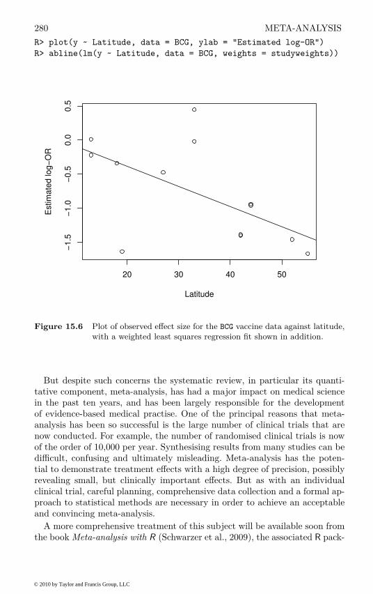
280 META-ANALYSIS
R> plot(y ~ Latitude, data = BCG, ylab = "Estimated log-OR")
R> abline(lm(y ~ Latitude, data = BCG, weights = studyweights))
20 30 40 50
−1
.5−
1.0
−0
.50
.00
.5
Latitude
Estim
ate
d lo
g−
OR
Figure 15.6 Plot of observed effect size for the BCG vaccine data against latitude,with a weighted least squares regression fit shown in addition.
But despite such concerns the systematic review, in particular its quanti-tative component, meta-analysis, has had a major impact on medical sciencein the past ten years, and has been largely responsible for the developmentof evidence-based medical practise. One of the principal reasons that meta-analysis has been so successful is the large number of clinical trials that arenow conducted. For example, the number of randomised clinical trials is nowof the order of 10,000 per year. Synthesising results from many studies can bedifficult, confusing and ultimately misleading. Meta-analysis has the poten-tial to demonstrate treatment effects with a high degree of precision, possiblyrevealing small, but clinically important effects. But as with an individualclinical trial, careful planning, comprehensive data collection and a formal ap-proach to statistical methods are necessary in order to achieve an acceptableand convincing meta-analysis.
A more comprehensive treatment of this subject will be available soon fromthe book Meta-analysis with R (Schwarzer et al., 2009), the associated R pack-
© 2010 by Taylor and Francis Group, LLC
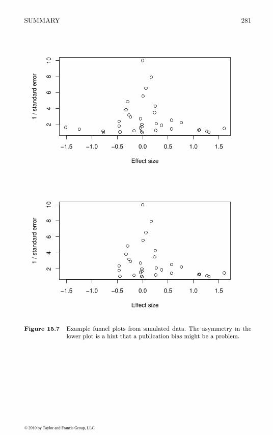
SUMMARY 281
−1.5 −1.0 −0.5 0.0 0.5 1.0 1.5
24
68
10
Effect size
1 /
sta
nd
ard
err
or
−1.5 −1.0 −0.5 0.0 0.5 1.0 1.5
24
68
10
Effect size
1 /
sta
nd
ard
err
or
Figure 15.7 Example funnel plots from simulated data. The asymmetry in thelower plot is a hint that a publication bias might be a problem.
© 2010 by Taylor and Francis Group, LLC
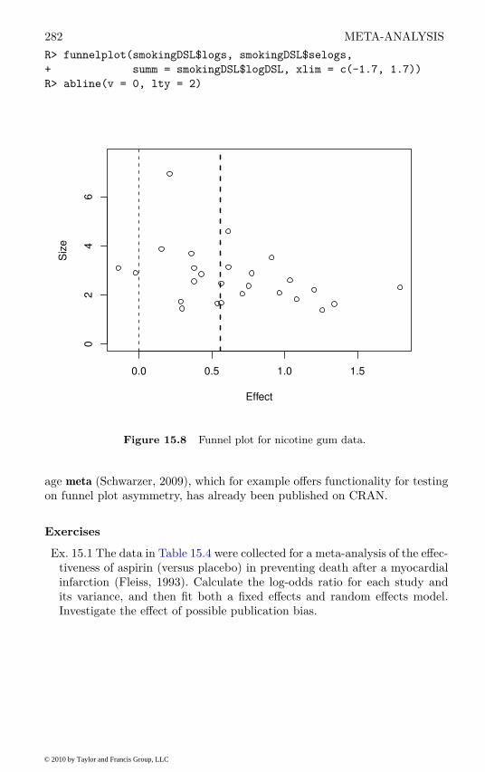
282 META-ANALYSIS
R> funnelplot(smokingDSL$logs, smokingDSL$selogs,
+ summ = smokingDSL$logDSL, xlim = c(-1.7, 1.7))
R> abline(v = 0, lty = 2)
0.0 0.5 1.0 1.5
02
46
Effect
Siz
e
Figure 15.8 Funnel plot for nicotine gum data.
age meta (Schwarzer, 2009), which for example offers functionality for testingon funnel plot asymmetry, has already been published on CRAN.
Exercises
Ex. 15.1 The data in Table 15.4 were collected for a meta-analysis of the effec-tiveness of aspirin (versus placebo) in preventing death after a myocardialinfarction (Fleiss, 1993). Calculate the log-odds ratio for each study andits variance, and then fit both a fixed effects and random effects model.Investigate the effect of possible publication bias.
© 2010 by Taylor and Francis Group, LLC
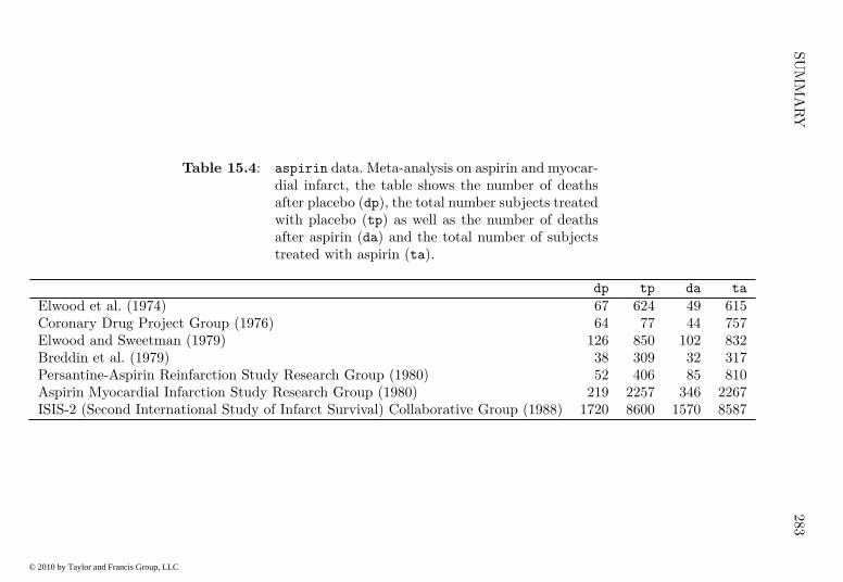
SU
MM
AR
Y28
3
Table 15.4: aspirin data. Meta-analysis on aspirin and myocar-dial infarct, the table shows the number of deathsafter placebo (dp), the total number subjects treatedwith placebo (tp) as well as the number of deathsafter aspirin (da) and the total number of subjectstreated with aspirin (ta).
dp tp da ta
Elwood et al. (1974) 67 624 49 615Coronary Drug Project Group (1976) 64 77 44 757Elwood and Sweetman (1979) 126 850 102 832Breddin et al. (1979) 38 309 32 317Persantine-Aspirin Reinfarction Study Research Group (1980) 52 406 85 810Aspirin Myocardial Infarction Study Research Group (1980) 219 2257 346 2267ISIS-2 (Second International Study of Infarct Survival) Collaborative Group (1988) 1720 8600 1570 8587
© 2010 by Taylor and Francis Group, LLC

284 META-ANALYSIS
Ex. 15.2 The data in Table 15.5 show the results of nine randomised trialscomparing two different toothpastes for the prevention of caries develop-ment (see Everitt and Pickles, 2000). The outcomes in each trial was thechange from baseline, in the decayed, missing (due to caries) and filledsurface dental index (DMFS). Calculate an appropriate measure of effectsize for each study and then carry out a meta-analysis of the results. Whatconclusions do you draw from the results?
Table 15.5: toothpaste data. Meta-analysis on trials comparingtwo toothpastes, the number of individuals in thestudy, the mean and the standard deviation for eachstudy A and B are shown.
Study nA meanA sdA nB meanB sdB
1 134 5.96 4.24 113 4.72 4.722 175 4.74 4.64 151 5.07 5.383 137 2.04 2.59 140 2.51 3.224 184 2.70 2.32 179 3.20 2.465 174 6.09 4.86 169 5.81 5.146 754 4.72 5.33 736 4.76 5.297 209 10.10 8.10 209 10.90 7.908 1151 2.82 3.05 1122 3.01 3.329 679 3.88 4.85 673 4.37 5.37
Ex. 15.3 As an exercise in writing R code write your own meta-analysisfunction that allows the plotting of observed effect sizes and their associatedconfidence intervals (forest plot), estimates the overall effect size and itsstandard error by both the fixed effects and random effect models, andshows both on the constructed forest plot.
© 2010 by Taylor and Francis Group, LLC

CHAPTER 16
Principal Component Analysis: TheOlympic Heptathlon
16.1 Introduction
The pentathlon for women was first held in Germany in 1928. Initially thisconsisted of the shot put, long jump, 100m, high jump and javelin events heldover two days. In the 1964 Olympic Games the pentathlon became the firstcombined Olympic event for women, consisting now of the 80m hurdles, shot,high jump, long jump and 200m. In 1977 the 200m was replaced by the 800mand from 1981 the IAAF brought in the seven-event heptathlon in place ofthe pentathlon, with day one containing the events 100m hurdles, shot, highjump, 200m and day two, the long jump, javelin and 800m. A scoring systemis used to assign points to the results from each event and the winner is thewoman who accumulates the most points over the two days. The event madeits first Olympic appearance in 1984.
In the 1988 Olympics held in Seoul, the heptathlon was won by one of thestars of women’s athletics in the USA, Jackie Joyner-Kersee. The results forall 25 competitors in all seven disciplines are given in Table 16.1 (from Handet al., 1994). We shall analyse these data using principal component analysis
with a view to exploring the structure of the data and assessing how thederived principal component scores (see later) relate to the scores assigned bythe official scoring system.
16.2 Principal Component Analysis
The basic aim of principal component analysis is to describe variation in aset of correlated variables, x1, x2, . . . , xq, in terms of a new set of uncorrelatedvariables, y1, y2, . . . , yq, each of which is a linear combination of the x variables.The new variables are derived in decreasing order of ‘importance’ in the sensethat y1 accounts for as much of the variation in the original data amongst alllinear combinations of x1, x2, . . . , xq. Then y2 is chosen to account for as muchas possible of the remaining variation, subject to being uncorrelated with y1
– and so on, i.e., forming an orthogonal coordinate system. The new variablesdefined by this process, y1, y2, . . . , yq, are the principal components.
The general hope of principal component analysis is that the first few com-ponents will account for a substantial proportion of the variation in the originalvariables, x1, x2, . . . , xq, and can, consequently, be used to provide a conve-
285
© 2010 by Taylor and Francis Group, LLC
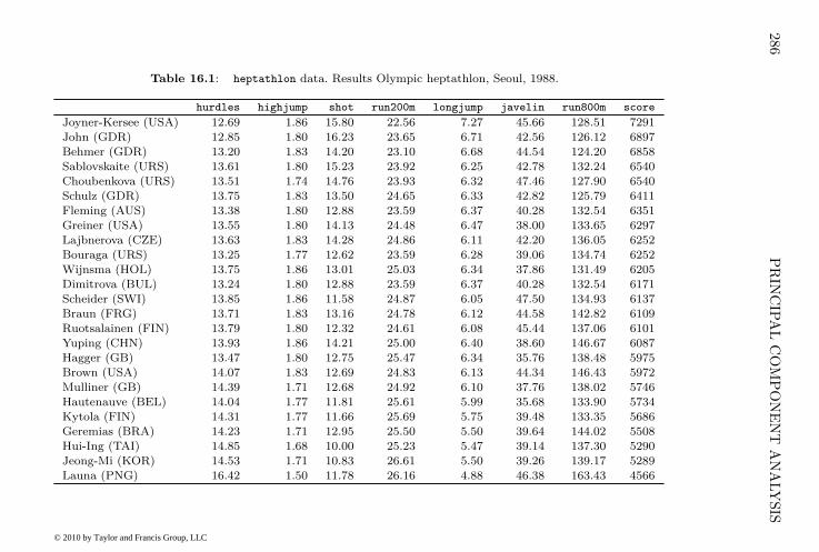
286
PR
INC
IPA
LC
OM
PO
NE
NT
AN
ALY
SIS
Table 16.1: heptathlon data. Results Olympic heptathlon, Seoul, 1988.
hurdles highjump shot run200m longjump javelin run800m score
Joyner-Kersee (USA) 12.69 1.86 15.80 22.56 7.27 45.66 128.51 7291
John (GDR) 12.85 1.80 16.23 23.65 6.71 42.56 126.12 6897
Behmer (GDR) 13.20 1.83 14.20 23.10 6.68 44.54 124.20 6858
Sablovskaite (URS) 13.61 1.80 15.23 23.92 6.25 42.78 132.24 6540
Choubenkova (URS) 13.51 1.74 14.76 23.93 6.32 47.46 127.90 6540
Schulz (GDR) 13.75 1.83 13.50 24.65 6.33 42.82 125.79 6411
Fleming (AUS) 13.38 1.80 12.88 23.59 6.37 40.28 132.54 6351
Greiner (USA) 13.55 1.80 14.13 24.48 6.47 38.00 133.65 6297
Lajbnerova (CZE) 13.63 1.83 14.28 24.86 6.11 42.20 136.05 6252
Bouraga (URS) 13.25 1.77 12.62 23.59 6.28 39.06 134.74 6252
Wijnsma (HOL) 13.75 1.86 13.01 25.03 6.34 37.86 131.49 6205
Dimitrova (BUL) 13.24 1.80 12.88 23.59 6.37 40.28 132.54 6171
Scheider (SWI) 13.85 1.86 11.58 24.87 6.05 47.50 134.93 6137
Braun (FRG) 13.71 1.83 13.16 24.78 6.12 44.58 142.82 6109
Ruotsalainen (FIN) 13.79 1.80 12.32 24.61 6.08 45.44 137.06 6101
Yuping (CHN) 13.93 1.86 14.21 25.00 6.40 38.60 146.67 6087
Hagger (GB) 13.47 1.80 12.75 25.47 6.34 35.76 138.48 5975
Brown (USA) 14.07 1.83 12.69 24.83 6.13 44.34 146.43 5972
Mulliner (GB) 14.39 1.71 12.68 24.92 6.10 37.76 138.02 5746
Hautenauve (BEL) 14.04 1.77 11.81 25.61 5.99 35.68 133.90 5734
Kytola (FIN) 14.31 1.77 11.66 25.69 5.75 39.48 133.35 5686
Geremias (BRA) 14.23 1.71 12.95 25.50 5.50 39.64 144.02 5508
Hui-Ing (TAI) 14.85 1.68 10.00 25.23 5.47 39.14 137.30 5290
Jeong-Mi (KOR) 14.53 1.71 10.83 26.61 5.50 39.26 139.17 5289
Launa (PNG) 16.42 1.50 11.78 26.16 4.88 46.38 163.43 4566
© 2010 by Taylor and Francis Group, LLC

PRINCIPAL COMPONENT ANALYSIS 287
nient lower-dimensional summary of these variables that might prove usefulfor a variety of reasons.
In some applications, the principal components may be an end in themselvesand might be amenable to interpretation in a similar fashion as the factors inan exploratory factor analysis (see Everitt and Dunn, 2001). More often theyare obtained for use as a means of constructing a low-dimensional informativegraphical representation of the data, or as input to some other analysis.
The low-dimensional representation produced by principal component anal-ysis is such that
n∑
r=1
n∑
s=1
(
d2
rs − d2
rs
)
is minimised with respect to d2rs. In this expression, drs is the Euclidean dis-
tance (see Chapter 17) between observations r and s in the original q dimen-
sional space, and drs is the corresponding distance in the space of the first m
components.As stated previously, the first principal component of the observations is
that linear combination of the original variables whose sample variance isgreatest amongst all possible such linear combinations. The second principalcomponent is defined as that linear combination of the original variables thataccounts for a maximal proportion of the remaining variance subject to beinguncorrelated with the first principal component. Subsequent components aredefined similarly. The question now arises as to how the coefficients specifyingthe linear combinations of the original variables defining each component arefound? The algebra of sample principal components is summarised briefly.
The first principal component of the observations, y1, is the linear combi-nation
y1 = a11x1 + a12x2 + . . . , a1qxq
whose sample variance is greatest among all such linear combinations. Sincethe variance of y1 could be increased without limit simply by increasing thecoefficients a⊤
1 = (a11, a12, . . . , a1q) (here written in form of a vector for conve-nience), a restriction must be placed on these coefficients. As we shall see later,a sensible constraint is to require that the sum of squares of the coefficients,a⊤
1 a1, should take the value one, although other constraints are possible.The second principal component y2 = a⊤
2 x with x = (x1, . . . , xq) is the lin-ear combination with greatest variance subject to the two conditions a⊤
2 a2 = 1and a⊤
2 a1 = 0. The second condition ensures that y1 and y2 are uncorrelated.Similarly, the jth principal component is that linear combination yj = a⊤
j x
which has the greatest variance subject to the conditions a⊤
j aj = 1 and
a⊤
j ai = 0 for (i < j).To find the coefficients defining the first principal component we need to
choose the elements of the vector a1 so as to maximise the variance of y1
subject to the constraint a⊤
1 a1 = 1.
© 2010 by Taylor and Francis Group, LLC

288 PRINCIPAL COMPONENT ANALYSIS
To maximise a function of several variables subject to one or more con-straints, the method of Lagrange multipliers is used. In this case this leadsto the solution that a1 is the eigenvector of the sample covariance matrix,S, corresponding to its largest eigenvalue – full details are given in Morrison(2005).
The other components are derived in similar fashion, with aj being theeigenvector of S associated with its jth largest eigenvalue. If the eigenvaluesof S are λ1, λ2, . . . , λq, then since a⊤
j aj = 1, the variance of the jth componentis given by λj .
The total variance of the q principal components will equal the total varianceof the original variables so that
q∑
j=1
λj = s2
1 + s2
2 + · · · + s2
q
where s2j is the sample variance of xj . We can write this more concisely as
q∑
j=1
λj = trace(S).
Consequently, the jth principal component accounts for a proportion Pj ofthe total variation of the original data, where
Pj =λj
trace(S).
The first m principal components, where m < q, account for a proportion
P (m) =
m∑
j=1
λj
trace(S).
When the variables are on very different scales principal component analysis isusally carried out on the correlation matrix rather than the covariance matrix.
16.3 Analysis Using R
To begin it will help to score all seven events in the same direction, so that‘large’ values are ‘good’. We will recode the running events to achieve this;
R> data("heptathlon", package = "HSAUR2")
R> heptathlon$hurdles <- max(heptathlon$hurdles) -
+ heptathlon$hurdles
R> heptathlon$run200m <- max(heptathlon$run200m) -
+ heptathlon$run200m
R> heptathlon$run800m <- max(heptathlon$run800m) -
+ heptathlon$run800m
Figure 16.1 shows a scatterplot matrix of the results from all 25 competitorsfor the seven events. Most of the scatterplots in the diagram suggest that there
© 2010 by Taylor and Francis Group, LLC

ANALYSIS USING R 289
R> score <- which(colnames(heptathlon) == "score")
R> plot(heptathlon[,-score])
hurdles
1.50 1.75 0 2 4 36 42
02
1.5
01.7
5
highjump
shot
10
13
16
02
4
run200m
longjump
5.0
6.5
36
42 javelin
0 2 10 13 16 5.0 6.5 0 20 40
020
40
run800m
Figure 16.1 Scatterplot matrix for the heptathlon data (all countries).
is a positive relationship between the results for each pairs of events. Theexception are the plots involving the javelin event which give little evidenceof any relationship between the result for this event and the results from theother six events; we will suggest possible reasons for this below, but first wewill examine the numerical values of the between pairs events correlations byapplying the cor function
R> round(cor(heptathlon[,-score]), 2)
hurdles highjump shot run200m longjump javelin run800m
hurdles 1.00 0.81 0.65 0.77 0.91 0.01 0.78
highjump 0.81 1.00 0.44 0.49 0.78 0.00 0.59
shot 0.65 0.44 1.00 0.68 0.74 0.27 0.42
run200m 0.77 0.49 0.68 1.00 0.82 0.33 0.62
© 2010 by Taylor and Francis Group, LLC

290 PRINCIPAL COMPONENT ANALYSIS
longjump 0.91 0.78 0.74 0.82 1.00 0.07 0.70
javelin 0.01 0.00 0.27 0.33 0.07 1.00 -0.02
run800m 0.78 0.59 0.42 0.62 0.70 -0.02 1.00
Examination of these numerical values confirms that most pairs of events arepositively correlated, some moderately (for example, high jump and shot) andothers relatively highly (for example, high jump and hurdles). And we see thatthe correlations involving the javelin event are all close to zero. One possibleexplanation for the latter finding is perhaps that training for the other sixevents does not help much in the javelin because it is essentially a ‘technical’event. An alternative explanation is found if we examine the scatterplot matrixin Figure 16.1 a little more closely. It is very clear in this diagram that forall events except the javelin there is an outlier, the competitor from PapuaNew Guinea (PNG), who is much poorer than the other athletes at these sixevents and who finished last in the competition in terms of points scored. Butsurprisingly in the scatterplots involving the javelin it is this competitor whoagain stands out but because she has the third highest value for the event.It might be sensible to look again at both the correlation matrix and thescatterplot matrix after removing the competitor from PNG; the relevant R
code is
R> heptathlon <- heptathlon[-grep("PNG", rownames(heptathlon)),]
Now, we again look at the scatterplot and correlation matrix;
R> round(cor(heptathlon[,-score]), 2)
hurdles highjump shot run200m longjump javelin run800m
hurdles 1.00 0.58 0.77 0.83 0.89 0.33 0.56
highjump 0.58 1.00 0.46 0.39 0.66 0.35 0.15
shot 0.77 0.46 1.00 0.67 0.78 0.34 0.41
run200m 0.83 0.39 0.67 1.00 0.81 0.47 0.57
longjump 0.89 0.66 0.78 0.81 1.00 0.29 0.52
javelin 0.33 0.35 0.34 0.47 0.29 1.00 0.26
run800m 0.56 0.15 0.41 0.57 0.52 0.26 1.00
The correlations change quite substantially and the new scatterplot matrix inFigure 16.2 does not point us to any further extreme observations. In the re-mainder of this chapter we analyse the heptathlon data with the observationsof the competitor from Papua New Guinea removed.
Because the results for the seven heptathlon events are on different scales weshall extract the principal components from the correlation matrix. A principalcomponent analysis of the data can be applied using the prcomp functionwith the scale argument set to TRUE to ensure the analysis is carried out onthe correlation matrix. The result is a list containing the coefficients definingeach component (sometimes referred to as loadings), the principal componentscores, etc. The required code is (omitting the score variable)
R> heptathlon_pca <- prcomp(heptathlon[, -score], scale = TRUE)
R> print(heptathlon_pca)
© 2010 by Taylor and Francis Group, LLC

ANALYSIS USING R 291
R> score <- which(colnames(heptathlon) == "score")
R> plot(heptathlon[,-score])
hurdles
1.70 1.85 0 2 4 36 42
1.5
3.0
1.7
01.8
5
highjump
shot
10
13
16
02
4
run200m
longjump
5.5
6.5
36
42 javelin
1.5 3.0 10 13 16 5.5 6.5 20 30 40
20
30
40
run800m
Figure 16.2 Scatterplot matrix for the heptathlon data after removing observa-
tions of the PNG competitor.
Standard deviations:
[1] 2.0793 0.9482 0.9109 0.6832 0.5462 0.3375 0.2620
Rotation:
PC1 PC2 PC3 PC4 PC5 PC6
hurdles -0.4504 0.05772 -0.1739 0.04841 -0.19889 0.84665
highjump -0.3145 -0.65133 -0.2088 -0.55695 0.07076 -0.09008
shot -0.4025 -0.02202 -0.1535 0.54827 0.67166 -0.09886
run200m -0.4271 0.18503 0.1301 0.23096 -0.61782 -0.33279
longjump -0.4510 -0.02492 -0.2698 -0.01468 -0.12152 -0.38294
javelin -0.2423 -0.32572 0.8807 0.06025 0.07874 0.07193
run800m -0.3029 0.65651 0.1930 -0.57418 0.31880 -0.05218
© 2010 by Taylor and Francis Group, LLC
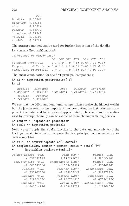
292 PRINCIPAL COMPONENT ANALYSIS
PC7
hurdles -0.06962
highjump 0.33156
shot 0.22904
run200m 0.46972
longjump -0.74941
javelin -0.21108
run800m 0.07719
The summary method can be used for further inspection of the details:
R> summary(heptathlon_pca)
Importance of components:
PC1 PC2 PC3 PC4 PC5 PC6 PC7
Standard deviation 2.1 0.9 0.9 0.68 0.55 0.34 0.26
Proportion of Variance 0.6 0.1 0.1 0.07 0.04 0.02 0.01
Cumulative Proportion 0.6 0.7 0.9 0.93 0.97 0.99 1.00
The linear combination for the first principal component is
R> a1 <- heptathlon_pca$rotation[,1]
R> a1
hurdles highjump shot run200m longjump
-0.4503876 -0.3145115 -0.4024884 -0.4270860 -0.4509639
javelin run800m
-0.2423079 -0.3029068
We see that the 200m and long jump competitions receive the highest weightbut the javelin result is less important. For computing the first principal com-ponent, the data need to be rescaled appropriately. The center and the scalingused by prcomp internally can be extracted from the heptathlon_pca via
R> center <- heptathlon_pca$center
R> scale <- heptathlon_pca$scale
Now, we can apply the scale function to the data and multiply with theloadings matrix in order to compute the first principal component score foreach competitor
R> hm <- as.matrix(heptathlon[,-score])
R> drop(scale(hm, center = center, scale = scale) %*%
+ heptathlon_pca$rotation[,1])
Joyner-Kersee (USA) John (GDR) Behmer (GDR)
-4.757530189 -3.147943402 -2.926184760
Sablovskaite (URS) Choubenkova (URS) Schulz (GDR)
-1.288135516 -1.503450994 -0.958467101
Fleming (AUS) Greiner (USA) Lajbnerova (CZE)
-0.953445060 -0.633239267 -0.381571974
Bouraga (URS) Wijnsma (HOL) Dimitrova (BUL)
-0.522322004 -0.217701500 -1.075984276
Scheider (SWI) Braun (FRG) Ruotsalainen (FIN)
0.003014986 0.109183759 0.208868056
© 2010 by Taylor and Francis Group, LLC
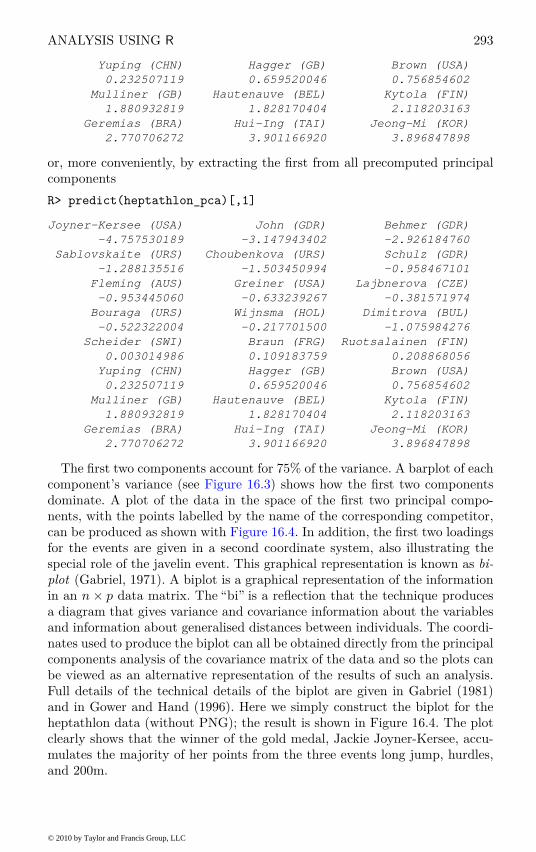
ANALYSIS USING R 293
Yuping (CHN) Hagger (GB) Brown (USA)
0.232507119 0.659520046 0.756854602
Mulliner (GB) Hautenauve (BEL) Kytola (FIN)
1.880932819 1.828170404 2.118203163
Geremias (BRA) Hui-Ing (TAI) Jeong-Mi (KOR)
2.770706272 3.901166920 3.896847898
or, more conveniently, by extracting the first from all precomputed principalcomponents
R> predict(heptathlon_pca)[,1]
Joyner-Kersee (USA) John (GDR) Behmer (GDR)
-4.757530189 -3.147943402 -2.926184760
Sablovskaite (URS) Choubenkova (URS) Schulz (GDR)
-1.288135516 -1.503450994 -0.958467101
Fleming (AUS) Greiner (USA) Lajbnerova (CZE)
-0.953445060 -0.633239267 -0.381571974
Bouraga (URS) Wijnsma (HOL) Dimitrova (BUL)
-0.522322004 -0.217701500 -1.075984276
Scheider (SWI) Braun (FRG) Ruotsalainen (FIN)
0.003014986 0.109183759 0.208868056
Yuping (CHN) Hagger (GB) Brown (USA)
0.232507119 0.659520046 0.756854602
Mulliner (GB) Hautenauve (BEL) Kytola (FIN)
1.880932819 1.828170404 2.118203163
Geremias (BRA) Hui-Ing (TAI) Jeong-Mi (KOR)
2.770706272 3.901166920 3.896847898
The first two components account for 75% of the variance. A barplot of eachcomponent’s variance (see Figure 16.3) shows how the first two componentsdominate. A plot of the data in the space of the first two principal compo-nents, with the points labelled by the name of the corresponding competitor,can be produced as shown with Figure 16.4. In addition, the first two loadingsfor the events are given in a second coordinate system, also illustrating thespecial role of the javelin event. This graphical representation is known as bi-
plot (Gabriel, 1971). A biplot is a graphical representation of the informationin an n × p data matrix. The “bi” is a reflection that the technique producesa diagram that gives variance and covariance information about the variablesand information about generalised distances between individuals. The coordi-nates used to produce the biplot can all be obtained directly from the principalcomponents analysis of the covariance matrix of the data and so the plots canbe viewed as an alternative representation of the results of such an analysis.Full details of the technical details of the biplot are given in Gabriel (1981)and in Gower and Hand (1996). Here we simply construct the biplot for theheptathlon data (without PNG); the result is shown in Figure 16.4. The plotclearly shows that the winner of the gold medal, Jackie Joyner-Kersee, accu-mulates the majority of her points from the three events long jump, hurdles,and 200m.
© 2010 by Taylor and Francis Group, LLC
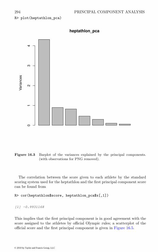
294 PRINCIPAL COMPONENT ANALYSIS
R> plot(heptathlon_pca)
heptathlon_pca
Va
ria
nce
s
01
23
4
Figure 16.3 Barplot of the variances explained by the principal components.
(with observations for PNG removed).
The correlation between the score given to each athlete by the standardscoring system used for the heptathlon and the first principal component scorecan be found from
R> cor(heptathlon$score, heptathlon_pca$x[,1])
[1] -0.9931168
This implies that the first principal component is in good agreement with thescore assigned to the athletes by official Olympic rules; a scatterplot of theofficial score and the first principal component is given in Figure 16.5.
© 2010 by Taylor and Francis Group, LLC

SUMMARY 295
R> biplot(heptathlon_pca, col = c("gray", "black"))
−0.4 −0.2 0.0 0.2 0.4 0.6
−0
.4−
0.3
−0
.2−
0.1
0.0
0.1
0.2
PC1
PC
2
Jy−K
John
Bhmr
Sblv
Chbn
SchlFlmn
Grnr
Ljbn
Borg
Wjns
Dmtr
Schd
Bran
Rtsl
Ypng
Hggr
Brwn
Mlln
Htnv
Kytl
Grms
H−In
Jn−M
−6 −4 −2 0 2 4 6 8
−4
−2
02
hurdles
highjump
shot
run200m
longjump
javelin
run800m
Figure 16.4 Biplot of the (scaled) first two principal components (with observa-
tions for PNG removed).
16.4 Summary
Principal components look for a few linear combinations of the original vari-ables that can be used to summarise a data set, losing in the process as littleinformation as possible. The derived variables might be used in a variety ofways, in particular for simplifying later analyses and providing informativeplots of the data. The method consists of transforming a set of correlated vari-ables to a new set of variables that are uncorrelated. Consequently it should benoted that if the original variables are themselves almost uncorrelated thereis little point in carrying out a principal components analysis, since it willmerely find components that are close to the original variables but arrangedin decreasing order of variance.
© 2010 by Taylor and Francis Group, LLC
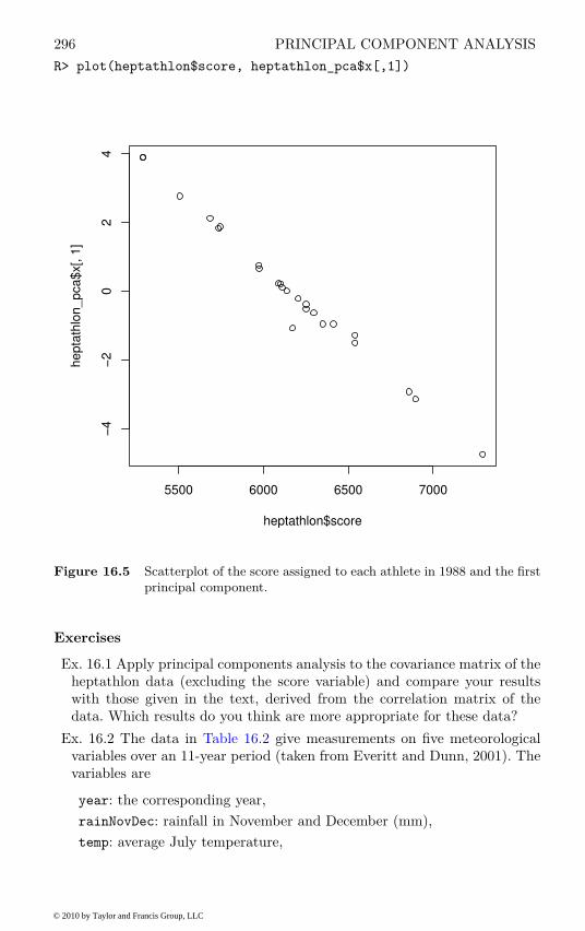
296 PRINCIPAL COMPONENT ANALYSIS
R> plot(heptathlon$score, heptathlon_pca$x[,1])
5500 6000 6500 7000
−4
−2
02
4
heptathlon$score
he
pta
thlo
n_
pca
$x[,
1]
Figure 16.5 Scatterplot of the score assigned to each athlete in 1988 and the first
principal component.
Exercises
Ex. 16.1 Apply principal components analysis to the covariance matrix of theheptathlon data (excluding the score variable) and compare your resultswith those given in the text, derived from the correlation matrix of thedata. Which results do you think are more appropriate for these data?
Ex. 16.2 The data in Table 16.2 give measurements on five meteorologicalvariables over an 11-year period (taken from Everitt and Dunn, 2001). Thevariables are
year: the corresponding year,
rainNovDec: rainfall in November and December (mm),
temp: average July temperature,
© 2010 by Taylor and Francis Group, LLC

SUMMARY 297
rainJuly: rainfall in July (mm),
radiation: radiation in July (curies), and
yield: average harvest yield (quintals per hectare).
Carry out a principal components analysis of both the covariance matrixand the correlation matrix of the data and compare the results. Which setof components leads to the most meaningful interpretation?
Table 16.2: meteo data. Meteorological measurements in an 11-year period.
year rainNovDec temp rainJuly radiation yield
1920-21 87.9 19.6 1.0 1661 28.371921-22 89.9 15.2 90.1 968 23.771922-23 153.0 19.7 56.6 1353 26.041923-24 132.1 17.0 91.0 1293 25.741924-25 88.8 18.3 93.7 1153 26.681925-26 220.9 17.8 106.9 1286 24.291926-27 117.7 17.8 65.5 1104 28.001927-28 109.0 18.3 41.8 1574 28.371928-29 156.1 17.8 57.4 1222 24.961929-30 181.5 16.8 140.6 902 21.661930-31 181.4 17.0 74.3 1150 24.37
Source: From Everitt, B. S. and Dunn, G., Applied Multivariate Data Anal-
ysis, 2nd Edition, Arnold, London, 2001. With permission.
Ex. 16.3 The correlations below are for the calculus measurements for the sixanterior mandibular teeth. Find all six principal components of the data anduse a screeplot to suggest how many components are needed to adequatelyaccount for the observed correlations. Can you interpret the components?
Table 16.3: Correlations for calculus measurements for the sixanterior mandibular teeth.
1.000.54 1.000.34 0.65 1.000.37 0.65 0.84 1.000.36 0.59 0.67 0.80 1.000.62 0.49 0.43 0.42 0.55 1.00
© 2010 by Taylor and Francis Group, LLC

CHAPTER 17
Multidimensional Scaling: BritishWater Voles and Voting in US
Congress
17.1 Introduction
Corbet et al. (1970) report a study of water voles (genus Arvicola) in whichthe aim was to compare British populations of these animals with those inEurope, to investigate whether more than one species might be present inBritain. The original data consisted of observations of the presence or absenceof 13 characteristics in about 300 water vole skulls arising from six Britishpopulations and eight populations from the rest of Europe. Table 17.1 gives adistance matrix derived from the data as described in Corbet et al. (1970).
Romesburg (1984) gives a set of data that shows the number of times 15 con-gressmen from New Jersey voted differently in the House of Representativeson 19 environmental bills. Abstentions are not recorded, but two congressmenabstained more frequently than the others, these being Sandman (nine absten-tions) and Thompson (six abstentions). The data are available in Table 17.2and of interest is if party affiliations can be detected.
17.2 Multidimensional Scaling
The data in Tables 17.1 and 17.2 are both examples of proximity matrices.The elements of such matrices attempt to quantify how similar are stimuli,objects, individuals, etc. In Table 17.1 the values measure the ‘distance’ be-tween populations of water voles; in Table 17.2 it is the similarity of the votingbehaviour of the congressmen that is measured. Models are fitted to proximi-ties in order to clarify, display and possibly explain any structure or patternnot readily apparent in the collection of numerical values. In some areas, par-ticularly psychology, the ultimate goal in the analysis of a set of proximitiesis more specifically theories for explaining similarity judgements, or in otherwords, finding an answer to the question “what makes things seem alike orseem different?”. Here though we will concentrate on how proximity data canbe best displayed to aid in uncovering any interesting structure.
The class of techniques we shall consider here, generally collected under thelabel multidimensional scaling (MDS), has the unifying feature that they seekto represent an observed proximity matrix by a simple geometrical model ormap. Such a model consists of a series of say q-dimensional coordinate values,
299
© 2010 by Taylor and Francis Group, LLC
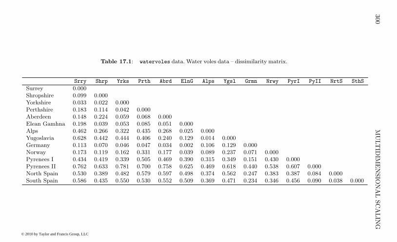
300
MU
LT
IDIM
EN
SIO
NA
LSC
AL
ING
Table 17.1: watervoles data. Water voles data – dissimilarity matrix.
Srry Shrp Yrks Prth Abrd ElnG Alps Ygsl Grmn Nrwy PyrI PyII NrtS SthS
Surrey 0.000Shropshire 0.099 0.000Yorkshire 0.033 0.022 0.000Perthshire 0.183 0.114 0.042 0.000Aberdeen 0.148 0.224 0.059 0.068 0.000Elean Gamhna 0.198 0.039 0.053 0.085 0.051 0.000Alps 0.462 0.266 0.322 0.435 0.268 0.025 0.000Yugoslavia 0.628 0.442 0.444 0.406 0.240 0.129 0.014 0.000Germany 0.113 0.070 0.046 0.047 0.034 0.002 0.106 0.129 0.000Norway 0.173 0.119 0.162 0.331 0.177 0.039 0.089 0.237 0.071 0.000Pyrenees I 0.434 0.419 0.339 0.505 0.469 0.390 0.315 0.349 0.151 0.430 0.000Pyrenees II 0.762 0.633 0.781 0.700 0.758 0.625 0.469 0.618 0.440 0.538 0.607 0.000North Spain 0.530 0.389 0.482 0.579 0.597 0.498 0.374 0.562 0.247 0.383 0.387 0.084 0.000South Spain 0.586 0.435 0.550 0.530 0.552 0.509 0.369 0.471 0.234 0.346 0.456 0.090 0.038 0.000
© 2010 by Taylor and Francis Group, LLC
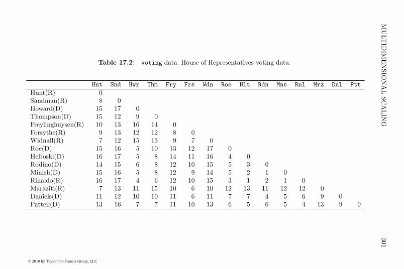
MU
LT
IDIM
EN
SIO
NA
LSC
AL
ING
301
Table 17.2: voting data. House of Representatives voting data.
Hnt Snd Hwr Thm Fry Frs Wdn Roe Hlt Rdn Mns Rnl Mrz Dnl Ptt
Hunt(R) 0Sandman(R) 8 0Howard(D) 15 17 0Thompson(D) 15 12 9 0Freylinghuysen(R) 10 13 16 14 0Forsythe(R) 9 13 12 12 8 0Widnall(R) 7 12 15 13 9 7 0Roe(D) 15 16 5 10 13 12 17 0Heltoski(D) 16 17 5 8 14 11 16 4 0Rodino(D) 14 15 6 8 12 10 15 5 3 0Minish(D) 15 16 5 8 12 9 14 5 2 1 0Rinaldo(R) 16 17 4 6 12 10 15 3 1 2 1 0Maraziti(R) 7 13 11 15 10 6 10 12 13 11 12 12 0Daniels(D) 11 12 10 10 11 6 11 7 7 4 5 6 9 0Patten(D) 13 16 7 7 11 10 13 6 5 6 5 4 13 9 0
© 2010 by Taylor and Francis Group, LLC

302 MULTIDIMENSIONAL SCALING
n in number, where n is the number of rows (and columns) of the proximitymatrix, and an associated measure of distance between pairs of points. Eachpoint is used to represent one of the stimuli in the resulting spatial model forthe proximities and the objective of a multidimensional approach is to deter-mine both the dimensionality of the model (i.e., the value of q) that providesan adequate ‘fit’, and the positions of the points in the resulting q-dimensionalspace. Fit is judged by some numerical index of the correspondence betweenthe observed proximities and the inter-point distances. In simple terms thismeans that the larger the perceived distance or dissimilarity between twostimuli (or the smaller their similarity), the further apart should be the pointsrepresenting them in the final geometrical model.
A number of inter-point distance measures might be used, but by far themost common is Euclidean distance. For two points, i and j, with q-dimensionalcoordinate values, xi = (xi1, xi2, . . . , xiq) and xj = (xj1, xj2, . . . , xjq) the Eu-clidean distance is defined as
dij =
√
√
√
√
q∑
k=1
(xik − xjk)2.
Having decided on a suitable distance measure the problem now becomesone of estimating the coordinate values to represent the stimuli, and this isachieved by optimising the chosen goodness of fit index measuring how wellthe fitted distances match the observed proximities. A variety of optimisationschemes combined with a variety of goodness of fit indices leads to a variety ofMDS methods. For details see, for example, Everitt and Rabe-Hesketh (1997).Here we give a brief account of two methods, classical scaling and non-metric
scaling, which will then be used to analyse the two data sets described earlier.
17.2.1 Classical Multidimensional Scaling
Classical scaling provides one answer to how we estimate q, and the n, q-dimensional, coordinate values x1, x2, . . . , xn, from the observed proximitymatrix, based on the work of Young and Householder (1938). To begin wemust note that there is no unique set of coordinate values since the Euclideandistances involved are unchanged by shifting the whole configuration of pointsfrom one place to another, or by rotation or reflection of the configuration. Inother words, we cannot uniquely determine either the location or the orienta-tion of the configuration. The location problem is usually overcome by placingthe mean vector of the configuration at the origin. The orientation problemmeans that any configuration derived can be subjected to an arbitrary orthog-
onal transformation. Such transformations can often be used to facilitate theinterpretation of solutions as will be seen later.
To begin our account of the method we shall assume that the proximitymatrix we are dealing with is a matrix of Euclidean distances D derived froma raw data matrix, X. Previously we saw how to calculate Euclidean distances
© 2010 by Taylor and Francis Group, LLC
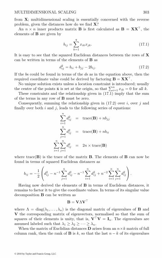
MULTIDIMENSIONAL SCALING 303
from X; multidimensional scaling is essentially concerned with the reverseproblem, given the distances how do we find X?
An n × n inner products matrix B is first calculated as B = XX⊤, theelements of B are given by
bij =
q∑
k=1
xikxjk. (17.1)
It is easy to see that the squared Euclidean distances between the rows of X
can be written in terms of the elements of B as
d2
ij = bii + bjj − 2bij . (17.2)
If the bs could be found in terms of the ds as in the equation above, then therequired coordinate value could be derived by factoring B = XX⊤.
No unique solution exists unless a location constraint is introduced; usuallythe centre of the points x is set at the origin, so that
∑n
i=1xik = 0 for all k.
These constraints and the relationship given in (17.1) imply that the sumof the terms in any row of B must be zero.
Consequently, summing the relationship given in (17.2) over i, over j andfinally over both i and j, leads to the following series of equations:
n∑
i=1
d2
ij = trace(B) + nbjj
n∑
j=1
d2
ij = trace(B) + nbii
n∑
i=1
n∑
j=1
d2
ij = 2n × trace(B)
where trace(B) is the trace of the matrix B. The elements of B can now befound in terms of squared Euclidean distances as
bij = −
1
2
d2
ij − n−1
n∑
j=1
d2
ij − n−1
n∑
i=1
d2
ij + n−2
n∑
i=1
n∑
j=1
d2
ij
.
Having now derived the elements of B in terms of Euclidean distances, itremains to factor it to give the coordinate values. In terms of its singular valuedecomposition B can be written as
B = VΛV⊤
where Λ = diag(λ1, . . . , λn) is the diagonal matrix of eigenvalues of B andV the corresponding matrix of eigenvectors, normalised so that the sum ofsquares of their elements is unity, that is, V⊤V = In. The eigenvalues areassumed labeled such that λ1 ≥ λ2 ≥ · · · ≥ λn.
When the matrix of Euclidian distances D arises from an n×k matrix of fullcolumn rank, then the rank of B is k, so that the last n− k of its eigenvalues
© 2010 by Taylor and Francis Group, LLC

304 MULTIDIMENSIONAL SCALING
will be zero. So B can be written as B = V1Λ1V⊤
1 , where V1 contains thefirst k eigenvectors and Λ1 the q non-zero eigenvalues. The required coordinate
values are thus X = V1Λ1/2
1, where Λ
1/2
1= diag(
√
λ1, . . . ,√
λk).The best fitting k-dimensional representation is given by the k eigenvec-
tors of B corresponding to the k largest eigenvalues. The adequacy of thek-dimensional representation can be judged by the size of the criterion
Pk =
k∑
i=1
λi
n−1∑
i=1
λi
.
Values of Pk of the order of 0.8 suggest a reasonable fit.When the observed dissimilarity matrix is not Euclidean, the matrix B is not
positive-definite. In such cases some of the eigenvalues of B will be negative;corresponding, some coordinate values will be complex numbers. If, however,B has only a small number of small negative eigenvalues, a useful represen-tation of the proximity matrix may still be possible using the eigenvectorsassociated with the k largest positive eigenvalues.
The adequacy of the resulting solution might be assessed using one of thefollowing two criteria suggested by Mardia et al. (1979); namely
k∑
i=1
|λi|
n∑
i=1
|λi|
or
k∑
i=1
λ2i
n∑
i=1
λ2i
.
Alternatively, Sibson (1979) recommends the following:
1. Trace criterion: Choose the number of coordinates so that the sum of theirpositive eigenvalues is approximately equal to the sum of all the eigenvalues.
2. Magnitude criterion: Accept as genuinely positive only those eigenvalueswhose magnitude substantially exceeds that of the largest negative eigen-value.
17.2.2 Non-metric Multidimensional Scaling
In classical scaling the goodness-of-fit measure is based on a direct numericalcomparison of observed proximities and fitted distances. In many situationshowever, it might be believed that the observed proximities contain little re-liable information beyond that implied by their rank order. In psychologicalexperiments, for example, proximity matrices frequently arise from asking sub-jects to make judgements about the similarity or dissimilarity of the stimuliof interest; in many such experiments the investigator may feel that, realisti-cally, subjects can give only ‘ordinal’ judgements. For example, in comparinga range of colours they might be able to specify that one was say ‘brighter’than another without being able to attach any realistic value to the extent
© 2010 by Taylor and Francis Group, LLC

ANALYSIS USING R 305
that they differed. For such situations, what is needed is a method of multidi-mensional scaling, the solutions from which depend only on the rank order ofthe proximities, rather than their actual numerical values. In other words thesolution should be invariant under monotonic transformations of the prox-imities. Such a method was originally suggested by Shepard (1962a,b) andKruskal (1964a). The quintessential component of the method is the use ofmonotonic regression (see Barlow et al., 1972). In essence the aim is to rep-
resent the fitted distances, dij , as dij = dij + εij where the disparities dij aremonotonic with the observed proximities and, subject to this constraint, re-semble the dij as closely as possible. Algorithms to achieve this are describedin Kruskal (1964b). For a given set of disparities the required coordinates canbe found by minimising some function of the squared differences between theobserved proximities and the derived disparities (generally known as stress inthis context). The procedure then iterates until some convergence criterion issatisfied. Again for details see Kruskal (1964b).
17.3 Analysis Using R
We can apply classical scaling to the distance matrix for populations of watervoles using the R function cmdscale. The following code finds the classicalscaling solution and computes the two criteria for assessing the required num-ber of dimensions as described above.
R> data("watervoles", package = "HSAUR2")
R> voles_mds <- cmdscale(watervoles, k = 13, eig = TRUE)
R> voles_mds$eig
[1] 7.359910e-01 2.626003e-01 1.492622e-01 6.990457e-02
[5] 2.956972e-02 1.931184e-02 8.326673e-17 -1.139451e-02
[9] -1.279569e-02 -2.849924e-02 -4.251502e-02 -5.255450e-02
[13] -7.406143e-02
Note that some of the eigenvalues are negative. The criterion P2 can be com-puted by
R> sum(abs(voles_mds$eig[1:2]))/sum(abs(voles_mds$eig))
[1] 0.6708889
and the criterion suggested by Mardia et al. (1979) is
R> sum((voles_mds$eig[1:2])^2)/sum((voles_mds$eig)^2)
[1] 0.9391378
The two criteria for judging number of dimensions differ considerably, but bothvalues are reasonably large, suggesting that the original distances between thewater vole populations can be represented adequately in two dimensions. Thetwo-dimensional solution can be plotted by extracting the coordinates fromthe points element of the voles_mds object; the plot is shown in Figure 17.1.
It appears that the six British populations are close to populations livingin the Alps, Yugoslavia, Germany, Norway and Pyrenees I (consisting of the
© 2010 by Taylor and Francis Group, LLC
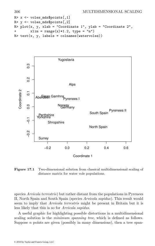
306 MULTIDIMENSIONAL SCALING
R> x <- voles_mds$points[,1]
R> y <- voles_mds$points[,2]
R> plot(x, y, xlab = "Coordinate 1", ylab = "Coordinate 2",
+ xlim = range(x)*1.2, type = "n")
R> text(x, y, labels = colnames(watervoles))
−0.2 0.0 0.2 0.4 0.6
−0
.2−
0.1
0.0
0.1
0.2
0.3
Coordinate 1
Co
ord
ina
te 2
Surrey
Shropshire
YorkshirePerthshire
AberdeenElean Gamhna
Alps
Yugoslavia
GermanyNorway
Pyrenees I
Pyrenees II
North Spain
South Spain
Figure 17.1 Two-dimensional solution from classical multidimensional scaling ofdistance matrix for water vole populations.
species Arvicola terrestris) but rather distant from the populations in PyreneesII, North Spain and South Spain (species Arvicola sapidus). This result wouldseem to imply that Arvicola terrestris might be present in Britain but it isless likely that this is so for Arvicola sapidus.
A useful graphic for highlighting possible distortions in a multidimensionalscaling solution is the minimum spanning tree, which is defined as follows.Suppose n points are given (possibly in many dimensions), then a tree span-
© 2010 by Taylor and Francis Group, LLC

ANALYSIS USING R 307
ning these points, i.e., a spanning tree, is any set of straight line segmentsjoining pairs of points such that
• No closed loops occur,
• Every point is visited at least one time,
• The tree is connected, i.e., it has paths between any pairs of points.
The length of the tree is defined to be the sum of the length of its segments,and when a set of n points and the length of all
(
n
2
)
segments are given, thenthe minimum spanning tree is defined as the spanning tree with minimumlength. Algorithms to find the minimum spanning tree of a set of n pointsgiven the distances between them are given in Prim (1957) and Gower andRoss (1969).
The links of the minimum spanning tree (of the spanning tree) of the prox-imity matrix of interest may be plotted onto the two-dimensional scaling rep-resentation in order to identify possible distortions produced by the scalingsolutions. Such distortions are indicated when nearby points on the plot arenot linked by an edge of the tree.
To find the minimum spanning tree of the water vole proximity matrix, thefunction mst from package ape (Paradis et al., 2009) can be used and we canplot the minimum spanning tree on the two-dimensional scaling solution asshown in Figure 17.2.
The plot indicates, for example, that the apparent closeness of the popula-tions in Germany and Norway, suggested by the points representing them inthe MDS solution, does not reflect accurately their calculated dissimilarity;the links of the minimum spanning tree show that the Aberdeen and EleanGamhna populations are actually more similar to the German water volesthan those from Norway.
We shall now apply non-metric scaling to the voting behaviour shown inTable 17.2. Non-metric scaling is available with function isoMDS from packageMASS (Venables and Ripley, 2002):
R> library("MASS")
R> data("voting", package = "HSAUR2")
R> voting_mds <- isoMDS(voting)
and we again depict the two-dimensional solution (Figure 17.3). The Figuresuggests that voting behaviour is essentially along party lines, although thereis more variation among Republicans. The voting behaviour of one of theRepublicans (Rinaldo) seems to be closer to his democratic colleagues ratherthan to the voting behaviour of other Republicans.
The quality of a multidimensional scaling can be assessed informally byplotting the original dissimilarities and the distances obtained from a mul-tidimensional scaling in a scatterplot, a so-called Shepard diagram. For thevoting data, such a plot is shown in Figure 17.4. In an ideal situation, thepoints fall on the bisecting line; in our case, some deviations are observable.
© 2010 by Taylor and Francis Group, LLC
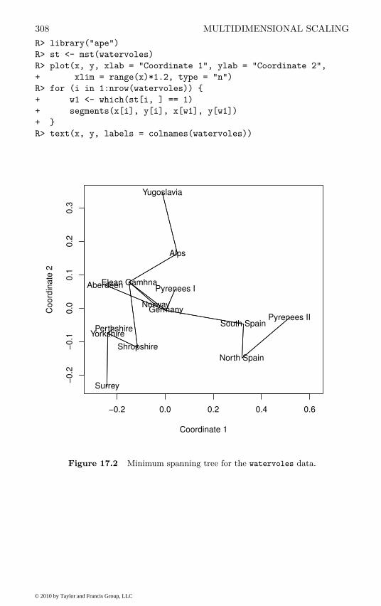
308 MULTIDIMENSIONAL SCALING
R> library("ape")
R> st <- mst(watervoles)
R> plot(x, y, xlab = "Coordinate 1", ylab = "Coordinate 2",
+ xlim = range(x)*1.2, type = "n")
R> for (i in 1:nrow(watervoles)) {
+ w1 <- which(st[i, ] == 1)
+ segments(x[i], y[i], x[w1], y[w1])
+ }
R> text(x, y, labels = colnames(watervoles))
−0.2 0.0 0.2 0.4 0.6
−0
.2−
0.1
0.0
0.1
0.2
0.3
Coordinate 1
Co
ord
ina
te 2
Surrey
Shropshire
YorkshirePerthshire
AberdeenElean Gamhna
Alps
Yugoslavia
GermanyNorway
Pyrenees I
Pyrenees II
North Spain
South Spain
Figure 17.2 Minimum spanning tree for the watervoles data.
© 2010 by Taylor and Francis Group, LLC
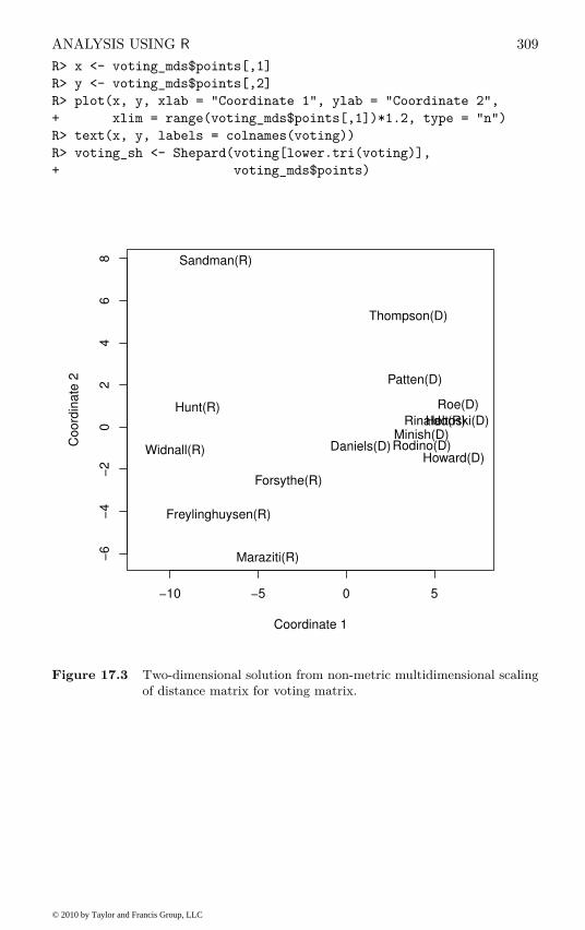
ANALYSIS USING R 309
R> x <- voting_mds$points[,1]
R> y <- voting_mds$points[,2]
R> plot(x, y, xlab = "Coordinate 1", ylab = "Coordinate 2",
+ xlim = range(voting_mds$points[,1])*1.2, type = "n")
R> text(x, y, labels = colnames(voting))
R> voting_sh <- Shepard(voting[lower.tri(voting)],
+ voting_mds$points)
−10 −5 0 5
−6
−4
−2
02
46
8
Coordinate 1
Co
ord
ina
te 2
Hunt(R)
Sandman(R)
Howard(D)
Thompson(D)
Freylinghuysen(R)
Forsythe(R)
Widnall(R)
Roe(D)
Heltoski(D)
Rodino(D)Minish(D)
Rinaldo(R)
Maraziti(R)
Daniels(D)
Patten(D)
Figure 17.3 Two-dimensional solution from non-metric multidimensional scalingof distance matrix for voting matrix.
© 2010 by Taylor and Francis Group, LLC
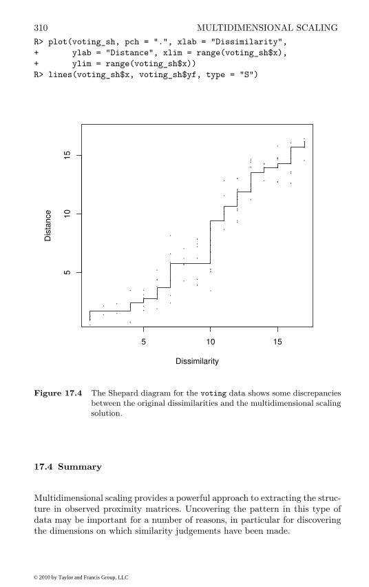
310 MULTIDIMENSIONAL SCALING
R> plot(voting_sh, pch = ".", xlab = "Dissimilarity",
+ ylab = "Distance", xlim = range(voting_sh$x),
+ ylim = range(voting_sh$x))
R> lines(voting_sh$x, voting_sh$yf, type = "S")
5 10 15
51
01
5
Dissimilarity
Dis
tan
ce
Figure 17.4 The Shepard diagram for the voting data shows some discrepanciesbetween the original dissimilarities and the multidimensional scalingsolution.
17.4 Summary
Multidimensional scaling provides a powerful approach to extracting the struc-ture in observed proximity matrices. Uncovering the pattern in this type ofdata may be important for a number of reasons, in particular for discoveringthe dimensions on which similarity judgements have been made.
© 2010 by Taylor and Francis Group, LLC

SUMMARY 311
Exercises
Ex. 17.1 The data in Table 17.3 shows road distances between 21 Europeancities. Apply classical scaling to the matrix and compare the plotted two-dimensional solution with a map of Europe.
Ex. 17.2 In Table 17.4 (from Kaufman and Rousseeuw, 1990), the dissim-ilarity matrix of 18 species of garden flowers is shown. Use some form ofmultidimensional scaling to investigate which species share common prop-erties.
Ex. 17.3 Consider 51 objects O1, . . . , O51 assumed to be arranged along astraight line with the jth object being located at a point with coordinatej. Define the similarity sij between object i and object j as
sij =
9 if i = j
8 if 1 ≤ |i − j| ≤ 37 if 4 ≤ |i − j| ≤ 6
· · ·
1 if 22 ≤ |i − j| ≤ 240 if |i − j| ≥ 25
Convert these similarities into dissimilarities (δij) by using
δij =√
sii + sjj − 2sij
and then apply classical multidimensional scaling to the resulting dissimi-laritiy matrix. Explain the shape of the derived two-dimensional solution.
© 2010 by Taylor and Francis Group, LLC
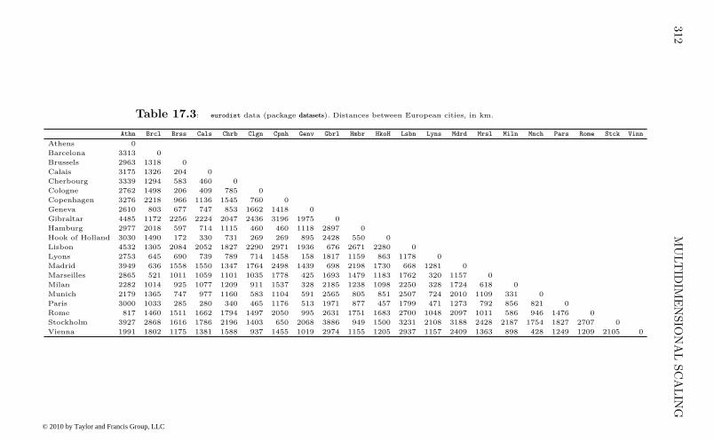
312
MU
LT
IDIM
EN
SIO
NA
LSC
AL
ING
Table 17.3: eurodist data (package datasets). Distances between European cities, in km.
Athn Brcl Brss Cals Chrb Clgn Cpnh Genv Gbrl Hmbr HkoH Lsbn Lyns Mdrd Mrsl Miln Mnch Pars Rome Stck Vinn
Athens 0
Barcelona 3313 0
Brussels 2963 1318 0
Calais 3175 1326 204 0
Cherbourg 3339 1294 583 460 0
Cologne 2762 1498 206 409 785 0
Copenhagen 3276 2218 966 1136 1545 760 0
Geneva 2610 803 677 747 853 1662 1418 0
Gibraltar 4485 1172 2256 2224 2047 2436 3196 1975 0
Hamburg 2977 2018 597 714 1115 460 460 1118 2897 0
Hook of Holland 3030 1490 172 330 731 269 269 895 2428 550 0
Lisbon 4532 1305 2084 2052 1827 2290 2971 1936 676 2671 2280 0
Lyons 2753 645 690 739 789 714 1458 158 1817 1159 863 1178 0
Madrid 3949 636 1558 1550 1347 1764 2498 1439 698 2198 1730 668 1281 0
Marseilles 2865 521 1011 1059 1101 1035 1778 425 1693 1479 1183 1762 320 1157 0
Milan 2282 1014 925 1077 1209 911 1537 328 2185 1238 1098 2250 328 1724 618 0
Munich 2179 1365 747 977 1160 583 1104 591 2565 805 851 2507 724 2010 1109 331 0
Paris 3000 1033 285 280 340 465 1176 513 1971 877 457 1799 471 1273 792 856 821 0
Rome 817 1460 1511 1662 1794 1497 2050 995 2631 1751 1683 2700 1048 2097 1011 586 946 1476 0
Stockholm 3927 2868 1616 1786 2196 1403 650 2068 3886 949 1500 3231 2108 3188 2428 2187 1754 1827 2707 0
Vienna 1991 1802 1175 1381 1588 937 1455 1019 2974 1155 1205 2937 1157 2409 1363 898 428 1249 1209 2105 0
© 2010 by Taylor and Francis Group, LLC
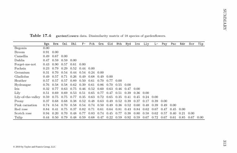
SU
MM
AR
Y31
3
Table 17.4: gardenflowers data. Dissimilarity matrix of 18 species of gardenflowers.
Bgn Brm Cml Dhl F- Fch Grn Gld Hth Hyd Irs Lly L- Pny Pnc Rdr Scr Tlp
Begonia 0.00
Broom 0.91 0.00
Camellia 0.49 0.67 0.00
Dahlia 0.47 0.59 0.59 0.00
Forget-me-not 0.43 0.90 0.57 0.61 0.00
Fuchsia 0.23 0.79 0.29 0.52 0.44 0.00
Geranium 0.31 0.70 0.54 0.44 0.54 0.24 0.00
Gladiolus 0.49 0.57 0.71 0.26 0.49 0.68 0.49 0.00
Heather 0.57 0.57 0.57 0.89 0.50 0.61 0.70 0.77 0.00
Hydrangae 0.76 0.58 0.58 0.62 0.39 0.61 0.86 0.70 0.55 0.00
Iris 0.32 0.77 0.63 0.75 0.46 0.52 0.60 0.63 0.46 0.47 0.00
Lily 0.51 0.69 0.69 0.53 0.51 0.65 0.77 0.47 0.51 0.39 0.36 0.00
Lily-of-the-valley 0.59 0.75 0.75 0.77 0.35 0.63 0.72 0.65 0.35 0.41 0.45 0.24 0.00
Peony 0.37 0.68 0.68 0.38 0.52 0.48 0.63 0.49 0.52 0.39 0.37 0.17 0.39 0.00
Pink carnation 0.74 0.54 0.70 0.58 0.54 0.74 0.50 0.49 0.36 0.52 0.60 0.48 0.39 0.49 0.00
Red rose 0.84 0.41 0.75 0.37 0.82 0.71 0.61 0.64 0.81 0.43 0.84 0.62 0.67 0.47 0.45 0.00
Scotch rose 0.94 0.20 0.70 0.48 0.77 0.83 0.74 0.45 0.77 0.38 0.80 0.58 0.62 0.57 0.40 0.21 0.00
Tulip 0.44 0.50 0.79 0.48 0.59 0.68 0.47 0.22 0.59 0.92 0.59 0.67 0.72 0.67 0.61 0.85 0.67 0.00
© 2010 by Taylor and Francis Group, LLC
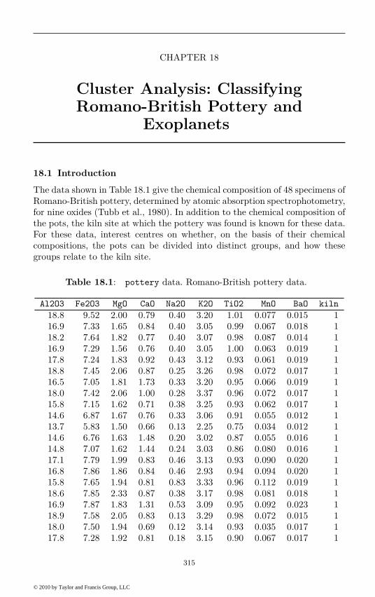
CHAPTER 18
Cluster Analysis: ClassifyingRomano-British Pottery and
Exoplanets
18.1 Introduction
The data shown in Table 18.1 give the chemical composition of 48 specimens ofRomano-British pottery, determined by atomic absorption spectrophotometry,for nine oxides (Tubb et al., 1980). In addition to the chemical composition ofthe pots, the kiln site at which the pottery was found is known for these data.For these data, interest centres on whether, on the basis of their chemicalcompositions, the pots can be divided into distinct groups, and how thesegroups relate to the kiln site.
Table 18.1: pottery data. Romano-British pottery data.
Al2O3 Fe2O3 MgO CaO Na2O K2O TiO2 MnO BaO kiln
18.8 9.52 2.00 0.79 0.40 3.20 1.01 0.077 0.015 116.9 7.33 1.65 0.84 0.40 3.05 0.99 0.067 0.018 118.2 7.64 1.82 0.77 0.40 3.07 0.98 0.087 0.014 116.9 7.29 1.56 0.76 0.40 3.05 1.00 0.063 0.019 117.8 7.24 1.83 0.92 0.43 3.12 0.93 0.061 0.019 118.8 7.45 2.06 0.87 0.25 3.26 0.98 0.072 0.017 116.5 7.05 1.81 1.73 0.33 3.20 0.95 0.066 0.019 118.0 7.42 2.06 1.00 0.28 3.37 0.96 0.072 0.017 115.8 7.15 1.62 0.71 0.38 3.25 0.93 0.062 0.017 114.6 6.87 1.67 0.76 0.33 3.06 0.91 0.055 0.012 113.7 5.83 1.50 0.66 0.13 2.25 0.75 0.034 0.012 114.6 6.76 1.63 1.48 0.20 3.02 0.87 0.055 0.016 114.8 7.07 1.62 1.44 0.24 3.03 0.86 0.080 0.016 117.1 7.79 1.99 0.83 0.46 3.13 0.93 0.090 0.020 116.8 7.86 1.86 0.84 0.46 2.93 0.94 0.094 0.020 115.8 7.65 1.94 0.81 0.83 3.33 0.96 0.112 0.019 118.6 7.85 2.33 0.87 0.38 3.17 0.98 0.081 0.018 116.9 7.87 1.83 1.31 0.53 3.09 0.95 0.092 0.023 118.9 7.58 2.05 0.83 0.13 3.29 0.98 0.072 0.015 118.0 7.50 1.94 0.69 0.12 3.14 0.93 0.035 0.017 117.8 7.28 1.92 0.81 0.18 3.15 0.90 0.067 0.017 1
315
© 2010 by Taylor and Francis Group, LLC
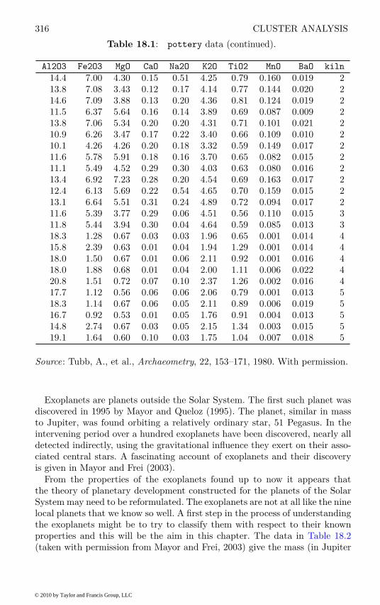
316 CLUSTER ANALYSIS
Table 18.1: pottery data (continued).
Al2O3 Fe2O3 MgO CaO Na2O K2O TiO2 MnO BaO kiln
14.4 7.00 4.30 0.15 0.51 4.25 0.79 0.160 0.019 213.8 7.08 3.43 0.12 0.17 4.14 0.77 0.144 0.020 214.6 7.09 3.88 0.13 0.20 4.36 0.81 0.124 0.019 211.5 6.37 5.64 0.16 0.14 3.89 0.69 0.087 0.009 213.8 7.06 5.34 0.20 0.20 4.31 0.71 0.101 0.021 210.9 6.26 3.47 0.17 0.22 3.40 0.66 0.109 0.010 210.1 4.26 4.26 0.20 0.18 3.32 0.59 0.149 0.017 211.6 5.78 5.91 0.18 0.16 3.70 0.65 0.082 0.015 211.1 5.49 4.52 0.29 0.30 4.03 0.63 0.080 0.016 213.4 6.92 7.23 0.28 0.20 4.54 0.69 0.163 0.017 212.4 6.13 5.69 0.22 0.54 4.65 0.70 0.159 0.015 213.1 6.64 5.51 0.31 0.24 4.89 0.72 0.094 0.017 211.6 5.39 3.77 0.29 0.06 4.51 0.56 0.110 0.015 311.8 5.44 3.94 0.30 0.04 4.64 0.59 0.085 0.013 318.3 1.28 0.67 0.03 0.03 1.96 0.65 0.001 0.014 415.8 2.39 0.63 0.01 0.04 1.94 1.29 0.001 0.014 418.0 1.50 0.67 0.01 0.06 2.11 0.92 0.001 0.016 418.0 1.88 0.68 0.01 0.04 2.00 1.11 0.006 0.022 420.8 1.51 0.72 0.07 0.10 2.37 1.26 0.002 0.016 417.7 1.12 0.56 0.06 0.06 2.06 0.79 0.001 0.013 518.3 1.14 0.67 0.06 0.05 2.11 0.89 0.006 0.019 516.7 0.92 0.53 0.01 0.05 1.76 0.91 0.004 0.013 514.8 2.74 0.67 0.03 0.05 2.15 1.34 0.003 0.015 519.1 1.64 0.60 0.10 0.03 1.75 1.04 0.007 0.018 5
Source: Tubb, A., et al., Archaeometry, 22, 153–171, 1980. With permission.
Exoplanets are planets outside the Solar System. The first such planet wasdiscovered in 1995 by Mayor and Queloz (1995). The planet, similar in massto Jupiter, was found orbiting a relatively ordinary star, 51 Pegasus. In theintervening period over a hundred exoplanets have been discovered, nearly alldetected indirectly, using the gravitational influence they exert on their asso-ciated central stars. A fascinating account of exoplanets and their discoveryis given in Mayor and Frei (2003).
From the properties of the exoplanets found up to now it appears thatthe theory of planetary development constructed for the planets of the SolarSystem may need to be reformulated. The exoplanets are not at all like the ninelocal planets that we know so well. A first step in the process of understandingthe exoplanets might be to try to classify them with respect to their knownproperties and this will be the aim in this chapter. The data in Table 18.2(taken with permission from Mayor and Frei, 2003) give the mass (in Jupiter
© 2010 by Taylor and Francis Group, LLC

INTRODUCTION 317
mass, mass), the period (in earth days, period) and the eccentricity (eccent)of the exoplanets discovered up until October 2002.
We shall investigate the structure of both the pottery data and the exo-planets data using a number of methods of cluster analysis.
Table 18.2: planets data. Jupiter mass, period and eccentricityof exoplanets.
mass period eccen mass period eccen
0.120 4.950000 0.0000 1.890 61.020000 0.10000.197 3.971000 0.0000 1.900 6.276000 0.15000.210 44.280000 0.3400 1.990 743.000000 0.62000.220 75.800000 0.2800 2.050 241.300000 0.24000.230 6.403000 0.0800 0.050 1119.000000 0.17000.250 3.024000 0.0200 2.080 228.520000 0.30400.340 2.985000 0.0800 2.240 311.300000 0.22000.400 10.901000 0.4980 2.540 1089.000000 0.06000.420 3.509700 0.0000 2.540 627.340000 0.06000.470 4.229000 0.0000 2.550 2185.000000 0.18000.480 3.487000 0.0500 2.630 414.000000 0.21000.480 22.090000 0.3000 2.840 250.500000 0.19000.540 3.097000 0.0100 2.940 229.900000 0.35000.560 30.120000 0.2700 3.030 186.900000 0.41000.680 4.617000 0.0200 3.320 267.200000 0.23000.685 3.524330 0.0000 3.360 1098.000000 0.22000.760 2594.000000 0.1000 3.370 133.710000 0.51100.770 14.310000 0.2700 3.440 1112.000000 0.52000.810 828.950000 0.0400 3.550 18.200000 0.01000.880 221.600000 0.5400 3.810 340.000000 0.36000.880 2518.000000 0.6000 3.900 111.810000 0.92700.890 64.620000 0.1300 4.000 15.780000 0.04600.900 1136.000000 0.3300 4.000 5360.000000 0.16000.930 3.092000 0.0000 4.120 1209.900000 0.65000.930 14.660000 0.0300 4.140 3.313000 0.02000.990 39.810000 0.0700 4.270 1764.000000 0.35300.990 500.730000 0.1000 4.290 1308.500000 0.31000.990 872.300000 0.2800 4.500 951.000000 0.45001.000 337.110000 0.3800 4.800 1237.000000 0.51501.000 264.900000 0.3800 5.180 576.000000 0.71001.010 540.400000 0.5200 5.700 383.000000 0.07001.010 1942.000000 0.4000 6.080 1074.000000 0.01101.020 10.720000 0.0440 6.292 71.487000 0.12431.050 119.600000 0.3500 7.170 256.000000 0.70001.120 500.000000 0.2300 7.390 1582.000000 0.47801.130 154.800000 0.3100 7.420 116.700000 0.4000
© 2010 by Taylor and Francis Group, LLC
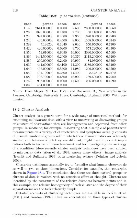
318 CLUSTER ANALYSIS
Table 18.2: planets data (continued).
mass period eccen mass period eccen
1.150 2614.000000 0.0000 7.500 2300.000000 0.39501.230 1326.000000 0.1400 7.700 58.116000 0.52901.240 391.000000 0.4000 7.950 1620.000000 0.22001.240 435.600000 0.4500 8.000 1558.000000 0.31401.282 7.126200 0.1340 8.640 550.650000 0.71001.420 426.000000 0.0200 9.700 653.220000 0.41001.550 51.610000 0.6490 10.000 3030.000000 0.56001.560 1444.500000 0.2000 10.370 2115.200000 0.62001.580 260.000000 0.2400 10.960 84.030000 0.33001.630 444.600000 0.4100 11.300 2189.000000 0.34001.640 406.000000 0.5300 11.980 1209.000000 0.37001.650 401.100000 0.3600 14.400 8.428198 0.27701.680 796.700000 0.6800 16.900 1739.500000 0.22801.760 903.000000 0.2000 17.500 256.030000 0.42901.830 454.000000 0.2000
Source: From Mayor, M., Frei, P.-Y., and Roukema, B., New Worlds in theCosmos, Cambridge University Press, Cambridge, England, 2003. With per-mission.
18.2 Cluster Analysis
Cluster analysis is a generic term for a wide range of numerical methods forexamining multivariate data with a view to uncovering or discovering groupsor clusters of observations that are homogeneous and separated from othergroups. In medicine, for example, discovering that a sample of patients withmeasurements on a variety of characteristics and symptoms actually consistsof a small number of groups within which these characteristics are relativelysimilar, and between which they are different, might have important impli-cations both in terms of future treatment and for investigating the aetiologyof a condition. More recently cluster analysis techniques have been appliedto microarray data (Alon et al., 1999, among many others), image analysis(Everitt and Bullmore, 1999) or in marketing science (Dolnicar and Leisch,2003).
Clustering techniques essentially try to formalise what human observers doso well in two or three dimensions. Consider, for example, the scatterplotshown in Figure 18.1. The conclusion that there are three natural groups orclusters of dots is reached with no conscious effort or thought. Clusters areidentified by the assessment of the relative distances between points and inthis example, the relative homogeneity of each cluster and the degree of theirseparation makes the task relatively simple.
Detailed accounts of clustering techniques are available in Everitt et al.(2001) and Gordon (1999). Here we concentrate on three types of cluster-
© 2010 by Taylor and Francis Group, LLC

CLUSTER ANALYSIS 319
0 5 10 15 20
02
46
81
0
x1
x2
Figure 18.1 Bivariate data showing the presence of three clusters.
ing procedures: agglomerative hierarchical clustering, k-means clustering andclassification maximum likelihood methods for clustering.
18.2.1 Agglomerative Hierarchical Clustering
In a hierarchical classification the data are not partitioned into a particularnumber of classes or clusters at a single step. Instead the classification consistsof a series of partitions that may run from a single ‘cluster’ containing allindividuals, to n clusters each containing a single individual. Agglomerativehierarchical clustering techniques produce partitions by a series of successivefusions of the n individuals into groups. With such methods, fusions, oncemade, are irreversible, so that when an agglomerative algorithm has placedtwo individuals in the same group they cannot subsequently appear in differentgroups. Since all agglomerative hierarchical techniques ultimately reduce thedata to a single cluster containing all the individuals, the investigator seeking
© 2010 by Taylor and Francis Group, LLC

320 CLUSTER ANALYSIS
the solution with the ‘best’ fitting number of clusters will need to decide whichdivision to choose. The problem of deciding on the ‘correct’ number of clusterswill be taken up later.
An agglomerative hierarchical clustering procedure produces a series of par-titions of the data, Pn, Pn−1, . . . , P1. The first, Pn, consists of n single-memberclusters, and the last, P1, consists of a single group containing all n individuals.The basic operation of all methods is similar:
Start Clusters C1, C2, . . . , Cn each containing a single individual.
Step 1 Find the nearest pair of distinct clusters, say Ci and Cj , merge Ci
and Cj , delete Cj and decrease the number of clusters by one.
Step 2 If number of clusters equals one then stop; else return to Step 1.
At each stage in the process the methods fuse individuals or groups ofindividuals that are closest (or most similar). The methods begin with aninter-individual distance matrix (for example, one containing Euclidean dis-tances), but as groups are formed, distance between an individual and a groupcontaining several individuals or between two groups of individuals will needto be calculated. How such distances are defined leads to a variety of differenttechniques; see the next sub-section.
Hierarchic classifications may be represented by a two-dimensional diagramknown as a dendrogram, which illustrates the fusions made at each stage of theanalysis. An example of such a diagram is given in Figure 18.2. The structureof Figure 18.2 resembles an evolutionary tree, a concept introduced by Darwinunder the term “Tree of Life” in his book On the Origin of Species by NaturalSelection in 1859 (see Figure 18.3), and it is in biological applications thathierarchical classifications are most relevant and most justified (although thistype of clustering has also been used in many other areas). According to Rohlf(1970), a biologist, all things being equal, aims for a system of nested clusters.Hawkins et al. (1982), however, issue the following caveat: “users should bevery wary of using hierarchic methods if they are not clearly necessary”.
18.2.2 Measuring Inter-cluster Dissimilarity
Agglomerative hierarchical clustering techniques differ primarily in how theymeasure the distance between or similarity of two clusters (where a clustermay, at times, consist of only a single individual). Two simple inter-groupmeasures are
dmin(A, B) = mini∈A,j∈B
dij
dmax(A, B) = maxi∈A,j∈B
dij
where d(A, B) is the distance between two clusters A and B, and dij is thedistance between individuals i and j. This could be Euclidean distance or oneof a variety of other distance measures (see Everitt et al., 2001, for details).
The inter-group dissimilarity measure dmin(A, B) is the basis of single link-
© 2010 by Taylor and Francis Group, LLC

CLUSTER ANALYSIS 321
9
3
4
10
2
7 8
5
1 6
Figure 18.2 Example of a dendrogram.
age clustering, dmax(A, B) that of complete linkage clustering. Both these tech-niques have the desirable property that they are invariant under monotonetransformations of the original inter-individual dissimilarities or distances. Afurther possibility for measuring inter-cluster distance or dissimilarity is
dmean(A, B) =1
|A| · |B|
∑
i∈A,j∈B
dij
where |A| and |B| are the number of individuals in clusters A and B. Thismeasure is the basis of a commonly used procedure known as average linkageclustering.
© 2010 by Taylor and Francis Group, LLC

© 2010 by Taylor and Francis Group, LLC© 2010 by Taylor and Francis Group, LLC

CLUSTER ANALYSIS 323
1. Find some initial partition of the individuals into the required number ofgroups. Such an initial partition could be provided by a solution from oneof the hierarchical clustering techniques described in the previous section.
2. Calculate the change in the clustering criterion produced by ‘moving’ eachindividual from its own to another cluster.
3. Make the change that leads to the greatest improvement in the value of theclustering criterion.
4. Repeat steps 2 and 3 until no move of an individual causes the clusteringcriterion to improve.
When variables are on very different scales (as they are for the exoplanetsdata) some form of standardisation will be needed before applying k-meansclustering (for a detailed discussion of this problem see Everitt et al., 2001).
18.2.4 Model-based Clustering
The k-means clustering method described in the previous section is basedlargely in heuristic but intuitively reasonable procedures. But it is not based onformal models thus making problems such as deciding on a particular method,estimating the number of clusters, etc., particularly difficult. And, of course,without a reasonable model, formal inference is precluded. In practise thesemay not be insurmountable objections to the use of the technique since clusteranalysis is essentially an ‘exploratory’ tool. But model-based cluster methodsdo have some advantages, and a variety of possibilities have been proposed.The most successful approach has been that proposed by Scott and Symons(1971) and extended by Banfield and Raftery (1993) and Fraley and Raftery(1999, 2002), in which it is assumed that the population from which the ob-servations arise consists of c subpopulations each corresponding to a cluster,and that the density of a q-dimensional observation x⊤ = (x1, . . . , xq) fromthe jth subpopulation is fj(x, ϑj), j = 1, . . . , c, for some unknown vector ofparameters, ϑj . They also introduce a vector γ = (γ1, . . . , γn), where γi = jof xi is from the j subpopulation. The γi label the subpopulation for eachobservation i = 1, . . . , n. The clustering problem now becomes that of choos-ing ϑ = (ϑ1, . . . , ϑc) and γ to maximise the likelihood function associatedwith such assumptions. This classification maximum likelihood procedure isdescribed briefly in the sequel.
18.2.5 Classification Maximum Likelihood
Assume the population consists of c subpopulations, each corresponding toa cluster of observations, and that the density function of a q-dimensionalobservation from the jth subpopulation is fj(x, ϑj) for some unknown vectorof parameters, ϑj . Also, assume that γ = (γ1, . . . , γn) gives the labels of thesubpopulation to which the observation belongs: so γi = j if xi is from thejth population.
© 2010 by Taylor and Francis Group, LLC
324 CLUSTER ANALYSIS
The clustering problem becomes that of choosing ϑ = (ϑ1, . . . , ϑc) and γ tomaximise the likelihood
L(ϑ, γ) =n
∏
i=1
fγi(xi, ϑγi
). (18.1)
If fj(x, ϑj) is taken as the multivariate normal density with mean vector µj
and covariance matrix Σj , this likelihood has the form
L(ϑ, γ) =c
∏
j=1
∏
i:γi=j
|Σj |−1/2 exp
(
−
1
2(xi − µj)⊤Σ−1
j (xi − µj)
)
. (18.2)
The maximum likelihood estimator of µj is µj = n−1
j
∑
i:γi=j xi where the
number of observations in each subpopulation is nj =∑n
i=1I(γi = j). Re-
placing µj in (18.2) yields the following log-likelihood
l(ϑ, γ) = −
1
2
c∑
j=1
trace(WjΣ−1
j ) + nj log |Σj |
where Wj is the q × q matrix of sums of squares and cross-products of thevariables for subpopulation j.
Banfield and Raftery (1993) demonstrate the following: If the covariancematrix Σj is σ2 times the identity matrix for all populations j = 1, . . . , c,then the likelihood is maximised by choosing γ to minimise trace(W), whereW =
∑cj=1
Wj , i.e., minimisation of the written group sum of squares. Useof this criterion in a cluster analysis will tend to produce spherical clusters oflargely equal sizes which may or may not match the ‘real’ clusters in the data.
If Σj = Σ for j = 1, . . . , c, then the likelihood is maximised by choosingγ to minimise |W|, a clustering criterion discussed by Friedman and Rubin(1967) and Marriott (1982). Use of this criterion in a cluster analysis willtend to produce clusters with the same elliptical shape, which again may notnecessarily match the actual clusters in the data.
If Σj is not constrained, the likelihood is maximised by choosing γ to min-imise
∑cj=1
nj log |Wj/nj |, a criterion that allows for different shaped clustersin the data.
Banfield and Raftery (1993) also consider criteria that allow the shape ofclusters to be less constrained than with the minimisation of trace(W) and|W| criteria, but to remain more parsimonious than the completely uncon-strained model. For example, constraining clusters to be spherical but not tohave the same volume, or constraining clusters to have diagonal covariancematrices but allowing their shapes, sizes and orientations to vary.
The EM algorithm (see Dempster et al., 1977) is used for maximum like-lihood estimation – details are given in Fraley and Raftery (1999). Modelselection is a combination of choosing the appropriate clustering model andthe optimal number of clusters. A Bayesian approach is used (see Fraley andRaftery, 1999), using what is known as the Bayesian Information Criterion(BIC).
© 2010 by Taylor and Francis Group, LLC

ANALYSIS USING R 325
18.3 Analysis Using R
18.3.1 Classifying Romano-British Pottery
We start our analysis with computing the dissimilarity matrix containing theEuclidean distance of the chemical measurements on all 45 pots. The resulting45 × 45 matrix can be inspected by an image plot, here obtained from func-tion levelplot available in package lattice (Sarkar, 2009, 2008). Such a plotassociates each cell of the dissimilarity matrix with a color or a grey value. Wechoose a very dark grey for cells with distance zero (i.e., the diagonal elementsof the dissimilarity matrix) and pale values for cells with greater Euclideandistance. Figure 18.4 leads to the impression that there are at least three dis-tinct groups with small inter-cluster differences (the dark rectangles) whereasmuch larger distances can be observed for all other cells.
We now construct three series of partitions using single, complete, and av-erage linkage hierarchical clustering as introduced in subsections 18.2.1 and18.2.2. The function hclust performs all three procedures based on the dis-similarity matrix of the data; its method argument is used to specify how thedistance between two clusters is assessed. The corresponding plot methoddraws a dendrogram; the code and results are given in Figure 18.5. Again, allthree dendrograms lead to the impression that three clusters fit the data best(although this judgement is very informal).
From the pottery_average object representing the average linkage hierar-chical clustering, we derive the three-cluster solution by cutting the dendro-gram at a height of four (which, based on the right display in Figure 18.5 leadsto a partition of the data into three groups). Our interest is now a comparisonwith the kiln sites at which the pottery was found.
R> pottery_cluster <- cutree(pottery_average, h = 4)
R> xtabs(~ pottery_cluster + kiln, data = pottery)
kiln
pottery_cluster 1 2 3 4 5
1 21 0 0 0 0
2 0 12 2 0 0
3 0 0 0 5 5
The contingency table shows that cluster 1 contains all pots found at kilnsite number one, cluster 2 contains all pots from kiln sites number two andthree, and cluster three collects the ten pots from kiln sites four and five. Infact, the five kiln sites are from three different regions defined by one, two andthree, and four and five, so the clusters actually correspond to pots from threedifferent regions.
18.3.2 Classifying Exoplanets
Prior to a cluster analysis we present a graphical representation of the three-dimensional planets data by means of the scatterplot3d package (Ligges and
© 2010 by Taylor and Francis Group, LLC
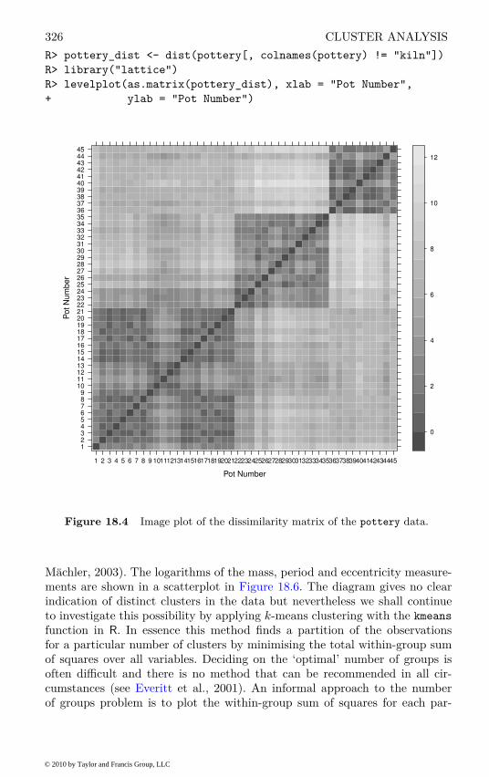
326 CLUSTER ANALYSIS
R> pottery_dist <- dist(pottery[, colnames(pottery) != "kiln"])
R> library("lattice")
R> levelplot(as.matrix(pottery_dist), xlab = "Pot Number",
+ ylab = "Pot Number")
Pot Number
Po
t N
um
be
r
123456789
101112131415161718192021222324252627282930313233343536373839404142434445
1 2 3 4 5 6 7 8 9 101112131415161718192021222324252627282930313233343536373839404142434445
0
2
4
6
8
10
12
Figure 18.4 Image plot of the dissimilarity matrix of the pottery data.
Machler, 2003). The logarithms of the mass, period and eccentricity measure-ments are shown in a scatterplot in Figure 18.6. The diagram gives no clearindication of distinct clusters in the data but nevertheless we shall continueto investigate this possibility by applying k-means clustering with the kmeans
function in R. In essence this method finds a partition of the observationsfor a particular number of clusters by minimising the total within-group sumof squares over all variables. Deciding on the ‘optimal’ number of groups isoften difficult and there is no method that can be recommended in all cir-cumstances (see Everitt et al., 2001). An informal approach to the numberof groups problem is to plot the within-group sum of squares for each par-
© 2010 by Taylor and Francis Group, LLC
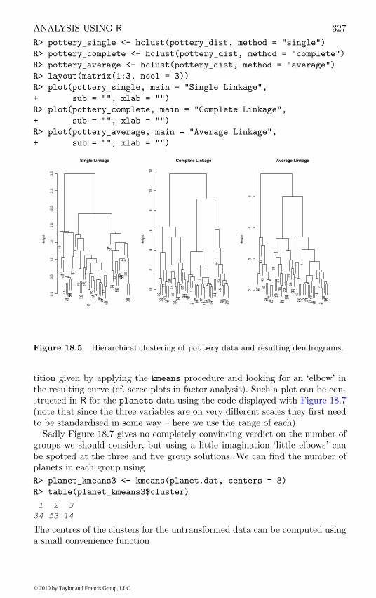
ANALYSIS USING R 327
R> pottery_single <- hclust(pottery_dist, method = "single")
R> pottery_complete <- hclust(pottery_dist, method = "complete")
R> pottery_average <- hclust(pottery_dist, method = "average")
R> layout(matrix(1:3, ncol = 3))
R> plot(pottery_single, main = "Single Linkage",
+ sub = "", xlab = "")
R> plot(pottery_complete, main = "Complete Linkage",
+ sub = "", xlab = "")
R> plot(pottery_average, main = "Average Linkage",
+ sub = "", xlab = "")
40
43
45
41
36
42
38
39
37
44
11
11
01
21
39
16
72 4
18
14
15 8 3
20 5
21
17
61
93
12
82
52
92
32
22
42
63
23
32
73
03
43
5
0.0
0.5
1.0
1.5
2.0
2.5
3.0
3.5
Single Linkage
He
igh
t
23
22
24
11
10
12
13
28
27
30
34
35
25
29
31
26
32
33
91
67
2 41
81
41
51
17
61
93
20 8
52
13
74
44
04
34
53
83
9 41
36
42
02
46
81
01
2
Complete Linkage
He
igh
t
37
44
40
43
45
38
39 4
13
64
22
82
52
92
73
03
43
52
32
22
43
12
63
23
31
11
01
21
31
32
0 85
21
17
61
99
16
72 4
18
14
15
02
46
Average Linkage
He
igh
t
Figure 18.5 Hierarchical clustering of pottery data and resulting dendrograms.
tition given by applying the kmeans procedure and looking for an ‘elbow’ inthe resulting curve (cf. scree plots in factor analysis). Such a plot can be con-structed in R for the planets data using the code displayed with Figure 18.7(note that since the three variables are on very different scales they first needto be standardised in some way – here we use the range of each).
Sadly Figure 18.7 gives no completely convincing verdict on the number ofgroups we should consider, but using a little imagination ‘little elbows’ canbe spotted at the three and five group solutions. We can find the number ofplanets in each group using
R> planet_kmeans3 <- kmeans(planet.dat, centers = 3)
R> table(planet_kmeans3$cluster)
1 2 3
34 53 14
The centres of the clusters for the untransformed data can be computed usinga small convenience function
© 2010 by Taylor and Francis Group, LLC

328 CLUSTER ANALYSIS
R> data("planets", package = "HSAUR2")
R> library("scatterplot3d")
R> scatterplot3d(log(planets$mass), log(planets$period),
+ log(planets$eccen), type = "h", angle = 55,
+ pch = 16, y.ticklabs = seq(0, 10, by = 2),
+ y.margin.add = 0.1, scale.y = 0.7)
−3 −2 −1 0 1 2 3
−5
−4
−3
−2
−1
0
0
2
4
6
8
10
log(planets$mass)
log
(pla
ne
ts$
pe
rio
d)
log
(pla
ne
ts$
ecce
n)
l
l
l
l
ll
l
l
ll
ll
l
l
l
l
l
l
l
ll
l
l
l
l
l
l
l
l
l
ll
l
l
l l
l
l
ll
ll
l
l
l
ll
l
ll
l l
l
l
l
l
l
l
ll
l
l
l
l
ll
l
l
l
ll
l
l
l
l
l
ll
l
l
l
l
l
l
l
l
l
l
l
l
l
l
l
l
Figure 18.6 3D scatterplot of the logarithms of the three variables available foreach of the exoplanets.
R> ccent <- function(cl) {
+ f <- function(i) colMeans(planets[cl == i,])
+ x <- sapply(sort(unique(cl)), f)
+ colnames(x) <- sort(unique(cl))
+ return(x)
+ }
which, applied to the three-cluster solution obtained by k-means gets
© 2010 by Taylor and Francis Group, LLC
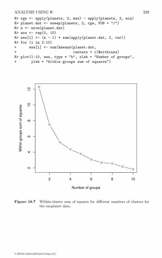
ANALYSIS USING R 329
R> rge <- apply(planets, 2, max) - apply(planets, 2, min)
R> planet.dat <- sweep(planets, 2, rge, FUN = "/")
R> n <- nrow(planet.dat)
R> wss <- rep(0, 10)
R> wss[1] <- (n - 1) * sum(apply(planet.dat, 2, var))
R> for (i in 2:10)
+ wss[i] <- sum(kmeans(planet.dat,
+ centers = i)$withinss)
R> plot(1:10, wss, type = "b", xlab = "Number of groups",
+ ylab = "Within groups sum of squares")
2 4 6 8 10
24
68
10
12
Number of groups
With
in g
rou
ps s
um
of
sq
ua
res
Figure 18.7 Within-cluster sum of squares for different numbers of clusters forthe exoplanet data.
© 2010 by Taylor and Francis Group, LLC

330 CLUSTER ANALYSIS
R> ccent(planet_kmeans3$cluster)
1 2 3
mass 2.9276471 1.6710566 10.56786
period 616.0760882 427.7105892 1693.17201
eccen 0.4953529 0.1219491 0.36650
for the three-cluster solution and, for the five cluster solution using
R> planet_kmeans5 <- kmeans(planet.dat, centers = 5)
R> table(planet_kmeans5$cluster)
1 2 3 4 5
18 35 14 30 4
R> ccent(planet_kmeans5$cluster)
1 2 3 4
mass 3.4916667 1.7448571 10.8121429 1.743533
period 638.0220556 552.3494286 1318.6505856 176.297374
eccen 0.6032778 0.2939143 0.3836429 0.049310
5
mass 2.115
period 3188.250
eccen 0.110
Interpretation of both the three- and five-cluster solutions clearly requiresa detailed knowledge of astronomy. But the mean vectors of the three-groupsolution, for example, imply a relatively large class of Jupiter-sized planetswith small periods and small eccentricities, a smaller class of massive planetswith moderate periods and large eccentricities, and a very small class of largeplanets with extreme periods and moderate eccentricities.
18.3.3 Model-based Clustering in R
We now proceed to apply model-based clustering to the planets data. R
functions for model-based clustering are available in package mclust (Fraleyet al., 2009, Fraley and Raftery, 2002). Here we use the Mclust function sincethis selects both the most appropriate model for the data and the optimalnumber of groups based on the values of the BIC computed over several modelsand a range of values for number of groups. The necessary code is:
R> library("mclust")
R> planet_mclust <- Mclust(planet.dat)
and we first examine a plot of BIC values using the R code that is displayedon top of Figure 18.8. In this diagram the different plotting symbols refer todifferent model assumptions about the shape of clusters:
EII: spherical, equal volume,
VII: spherical, unequal volume,
EEI: diagonal, equal volume and shape,
VEI: diagonal, varying volume, equal shape,
© 2010 by Taylor and Francis Group, LLC
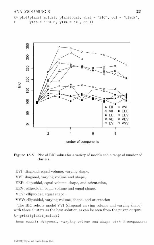
ANALYSIS USING R 331
R> plot(planet_mclust, planet.dat, what = "BIC", col = "black",
+ ylab = "-BIC", ylim = c(0, 350))
2 4 6 8
05
01
00
15
02
00
25
03
00
35
0
number of components
BIC
l
l l
l
l
l
l
l
l
l
EIIVIIEEIVEIEVI
VVIEEEEEVVEVVVV
Figure 18.8 Plot of BIC values for a variety of models and a range of number ofclusters.
EVI: diagonal, equal volume, varying shape,
VVI: diagonal, varying volume and shape,
EEE: ellipsoidal, equal volume, shape, and orientation,
EEV: ellipsoidal, equal volume and equal shape,
VEV: ellipsoidal, equal shape,
VVV: ellipsoidal, varying volume, shape, and orientation
The BIC selects model VVI (diagonal varying volume and varying shape)with three clusters as the best solution as can be seen from the print output:
R> print(planet_mclust)
best model: diagonal, varying volume and shape with 3 components
© 2010 by Taylor and Francis Group, LLC

332 CLUSTER ANALYSIS
R> clPairs(planet.dat,
+ classification = planet_mclust$classification,
+ symbols = 1:3, col = "black")
mass
0.0 0.2 0.4 0.6 0.8 1.0
0.0
0.2
0.4
0.6
0.8
1.0
0.0
0.2
0.4
0.6
0.8
1.0
period
0.0 0.2 0.4 0.6 0.8 1.0 0.0 0.2 0.4 0.6 0.8 1.0
0.0
0.2
0.4
0.6
0.8
1.0
eccen
Figure 18.9 Scatterplot matrix of planets data showing a three-cluster solutionfrom Mclust.
This solution can be shown graphically as a scatterplot matrix. The plot isshown in Figure 18.9. Figure 18.10 depicts the clustering solution in the three-dimensional space.
The number of planets in each cluster and the mean vectors of the threeclusters for the untransformed data can now be inspected by using
R> table(planet_mclust$classification)
1 2 3
19 41 41
R> ccent(planet_mclust$classification)
© 2010 by Taylor and Francis Group, LLC

ANALYSIS USING R 333
R> scatterplot3d(log(planets$mass), log(planets$period),
+ log(planets$eccen), type = "h", angle = 55,
+ scale.y = 0.7, pch = planet_mclust$classification,
+ y.ticklabs = seq(0, 10, by = 2), y.margin.add = 0.1)
−3 −2 −1 0 1 2 3
−5
−4
−3
−2
−1
0
0
2
4
6
8
10
log(planets$mass)
log
(pla
ne
ts$
pe
rio
d)
log
(pla
ne
ts$
ecce
n)
Figure 18.10 3D scatterplot of planets data showing a three-cluster solution fromMclust.
1 2 3
mass 1.16652632 1.5797561 6.0761463
period 6.47180158 313.4127073 1325.5310048
eccen 0.03652632 0.3061463 0.3704951
Cluster 1 consists of planets about the same size as Jupiter with very shortperiods and eccentricities (similar to the first cluster of the k-means solution).Cluster 2 consists of slightly larger planets with moderate periods and largeeccentricities, and cluster 3 contains the very large planets with very large pe-riods. These two clusters do not match those found by the k-means approach.
© 2010 by Taylor and Francis Group, LLC

334 CLUSTER ANALYSIS
18.4 Summary
Cluster analysis techniques provide a rich source of possible strategies for ex-ploring complex multivariate data. But the use of cluster analysis in practisedoes not involve simply the application of one particular technique to the dataunder investigation, but rather necessitates a series of steps, each of which maybe dependent on the results of the preceding one. It is generally impossiblea priori to anticipate what combination of variables, similarity measures andclustering technique is likely to lead to interesting and informative classifi-cations. Consequently, the analysis proceeds through several stages, with theresearcher intervening if necessary to alter variables, choose a different similar-ity measure, concentrate on a particular subset of individuals, and so on. Thefinal, extremely important, stage concerns the evaluation of the clustering so-lutions obtained. Are the clusters ‘real’ or merely artefacts of the algorithms?Do other solutions exist that are better in some sense? Can the clusters begiven a convincing interpretation? A long list of such questions might be posed,and readers intending to apply clustering to their data are recommended toread the detailed accounts of cluster evaluation given in Dubes and Jain (1979)and in Everitt et al. (2001).
Exercises
Ex. 18.1 Construct a three-dimensional drop-line scatterplot of the planetsdata in which the points are labelled with a suitable cluster label.
Ex. 18.2 Write an R function to fit a mixture of k normal densities to a dataset using maximum likelihood.
Ex. 18.3 Apply complete linkage and average linkage hierarchical clusteringto the planets data. Compare the results with those given in the text.
Ex. 18.4 Write a general R function that will display a particular partitionfrom the k-means cluster method on both a scatterplot matrix of the orig-inal data and a scatterplot or scatterplot matrix of a selected number ofprincipal components of the data.
© 2010 by Taylor and Francis Group, LLC

Bibliography
Adler, D. and Murdoch, D. (2009), rgl: 3D Visualization Device System
(OpenGL), URL http://rgl.neoscientists.org, R package version 0.84.
Agresti, A. (1996), An Introduction to Categorical Data Analysis, New York,USA: John Wiley & Sons.
Agresti, A. (2002), Categorical Data Analysis, Hoboken, New Jersey, USA:John Wiley & Sons, 2nd edition.
Aitkin, M. (1978), “The analysis of unbalanced cross-classifications,” Journal
of the Royal Statistical Society, Series A, 141, 195–223, with discussion.
Alon, U., Barkai, N., Notternam, D. A., Gish, K., Ybarra, S., Mack, D., andLevine, A. J. (1999), “Broad patterns of gene expressions revealed by clus-tering analysis of tumour and normal colon tissues probed by oligonucleotidearrays,” Cell Biology , 99, 6754–6760.
Ambler, G. and Benner, A. (2009), mfp: Multivariable Fractional Polynomi-
als, URL http://CRAN.R-project.org/package=mfp, R package version1.4.6.
Aspirin Myocardial Infarction Study Research Group (1980), “A randomized,controlled trial of aspirin in persons recovered from myocardial infarction,”Journal of the American Medical Association, 243, 661–669.
Bailey, K. R. (1987), “Inter-study differences: how should they influence theinterpretation of results?” Statistics in Medicine, 6, 351–360.
Banfield, J. D. and Raftery, A. E. (1993), “Model-based Gaussian and non-Gaussian clustering,” Biometrics, 49, 803–821.
Barlow, R. E., Bartholomew, D. J., Bremner, J. M., and Brunk, H. D. (1972),Statistical Inference under Order Restrictions, New York, USA: John Wiley& Sons.
Bates, D. (2005), “Fitting linear mixed models in R,” R News, 5, 27–30, URLhttp://CRAN.R-project.org/doc/Rnews/.
Bates, D. and Sarkar, D. (2008), lme4: Linear Mixed-Effects Models Using
S4 Classes, URL http://CRAN.R-project.org/package=lme4, R packageversion 0.999375-28.
Beck, A., Steer, R., and Brown, G. (1996), BDI-II Manual , The PsychologicalCorporation, San Antonio, 2nd edition.
Becker, R. A., Chambers, J. M., and Wilks, A. R. (1988), The New S Lan-
guage, London, UK: Chapman & Hall.
335
© 2010 by Taylor and Francis Group, LLC
336 BIBLIOGRAPHY
Bonsch, D., Lederer, T., Reulbach, U., Hothorn, T., Kornhuber, J., and Ble-ich, S. (2005), “Joint analysis of the NACP-REP1 marker within the al-pha synuclein gene concludes association with alcohol dependence,” Human
Molecular Genetics, 14, 967–971.
Breddin, K., Loew, D., Lechner, K., Uberla, K., and Walter, E. (1979),“Secondary prevention of myocardial infarction. Comparison of acetylsali-cylic acid, phenprocoumon and placebo. A multicenter two-year prospectivestudy,” Thrombosis and Haemostasis, 41, 225–236.
Breiman, L. (1996), “Bagging predictors,” Machine Learning , 24, 123–140.
Breiman, L. (2001a), “Random forests,” Machine Learning , 45, 5–32.
Breiman, L. (2001b), “Statistical modeling: The two cultures,” Statistical Sci-
ence, 16, 199–231, with discussion.
Breiman, L., Cutler, A., Liaw, A., and Wiener, M. (2009), randomForest:
Breiman and Cutler’s Random Forests for Classification and Regression,URL http://stat-www.berkeley.edu/users/breiman/RandomForests,R package version 4.5-30.
Breiman, L., Friedman, J. H., Olshen, R. A., and Stone, C. J. (1984), Classi-
fication and Regression Trees, California, USA: Wadsworth.
Buhlmann, P. (2004),“Bagging, boosting and ensemble methods,” in Handbook
of Computational Statistics, eds. J. E. Gentle, W. Hardle, and Y. Mori,Berlin, Heidelberg: Springer-Verlag, pp. 877–907.
Buhlmann, P. and Hothorn, T. (2007), “Boosting algorithms: Regularization,prediction and model fitting,” Statistical Science, 22, 477–505.
Canty, A. and Ripley, B. D. (2009), boot: Bootstrap R (S-PLUS) Functions,URL http://CRAN.R-project.org/package=boot, R package version 1.2-36.
Carey, V. J., Lumley, T., and Ripley, B. D. (2008), gee: Generalized Estima-
tion Equation Solver , URL http://CRAN.R-project.org/package=gee, Rpackage version 4.13-13.
Carlin, J. B., Ryan, L. M., Harvey, E. A., and Holmes, L. B. (2000), “Anticon-vulsant teratogenesis 4: Inter-rater agreement in assessing minor physicalfeatures related to anticonvulsant therapy,” Teratology , 62, 406–412.
Carpenter, J., Pocock, S., and Lamm, C. J. (2002), “Coping with missingdata in clinical trials: A model-based approach applied to asthma trials,”Statistics in Medicine, 21, 1043–1066.
Chalmers, T. C. and Lau, J. (1993), “Meta-analytic stimulus for changes inclinical trials,” Statistical Methods in Medical Research, 2, 161–172.
Chambers, J. M. (1998), Programming with Data, New York, USA: Springer-Verlag.
Chambers, J. M., Cleveland, W. S., Kleiner, B., and Tukey, P. A. (1983),Graphical Methods for Data Analysis, London: Chapman & Hall/CRC.
© 2010 by Taylor and Francis Group, LLC

BIBLIOGRAPHY 337
Chambers, J. M. and Hastie, T. J. (1992), Statistical Models in S , London,UK: Chapman & Hall.
Chen, C., Hardle, W., and Unwin, A., eds. (2008), Handbook of Data Visual-
ization, Berlin, Heidelberg: Springer-Verlag.
Cleveland, W. S. (1979), “Robust locally weighted regression and smoothingscatterplots,” Journal of the American Statistical Association, 74, 829–836.
Colditz, G. A., Brewer, T. F., Berkey, C. S., Wilson, M. E., Burdick, E.,Fineberg, H. V., and Mosteller, F. (1994), “Efficacy of BCG vaccine in theprevention of tuberculosis. Meta-analysis of the published literature,” Jour-
nal of the American Medical Association, 271, 698–702.
Collett, D. (2003), Modelling Binary Data, London, UK: Chapman &Hall/CRC, 2nd edition.
Collett, D. and Jemain, A. A. (1985), “Residuals, outliers and influential ob-servations in regression analysis,” Sains Malaysiana, 4, 493–511.
Cook, R. D. and Weisberg, S. (1982), Residuals and Influence in Regression,London, UK: Chapman & Hall/CRC.
Cook, R. J. (1998), “Generalized linear model,” in Encyclopedia of Biostatis-
tics, eds. P. Armitage and T. Colton, Chichester, UK: John Wiley & Sons.
Corbet, G. B., Cummins, J., Hedges, S. R., and Krzanowski, W. J. (1970),“The taxonomic structure of British water voles, genus Arvicola,” Journal
of Zoology , 61, 301–316.
Coronary Drug Project Group (1976), “Asprin in coronary heart disease,”Journal of Chronic Diseases, 29, 625–642.
Cox, D. R. (1972), “Regression models and life-tables,” Journal of the Royal
Statistical Society, Series B , 34, 187–202, with discussion.
Dalgaard, P. (2002), Introductory Statistics with R, New York, USA: Springer-Verlag.
Davis, C. S. (1991), “Semi-parametric and non-parametric methods for theanalysis of repeated measurements with applications to clinical trials,”Statistics in Medicine, 10, 1959–1980.
Davis, C. S. (2002), Statistical Methods for the Analysis of Repeated Measure-
ments, New York, USA: Springer-Verlag.
DeMets, D. L. (1987), “Methods for combining randomized clinical trials:strengths and limitations,” Statistics in Medicine, 6, 341–350.
Dempster, A. P., Laird, N. M., and Rubin, D. B. (1977), “Maximum likelihoodfrom incomplete data via the EM algorithm (C/R: p22-37),” Journal of the
Royal Statistical Society, Series B , 39, 1–22.
DerSimonian, R. and Laird, N. (1986), “Meta-analysis in clinical trials,” Con-
trolled Clinical Trials, 7, 177–188.
Diggle, P. J. (1998), “Dealing with missing values in longitudinal studies,”in Statistical Analysis of Medical Data, eds. B. S. Everitt and G. Dunn,London, UK: Arnold.
© 2010 by Taylor and Francis Group, LLC

338 BIBLIOGRAPHY
Diggle, P. J., Heagerty, P. J., Liang, K. Y., and Zeger, S. L. (2003), Analysis
of Longitudinal Data, Oxford, UK: Oxford University Press.
Diggle, P. J. and Kenward, M. G. (1994), “Informative dropout in longitudinaldata analysis,” Journal of the Royal Statistical Society, Series C , 43, 49–93.
Dolnicar, S. and Leisch, F. (2003), “Winter tourist segments in Austria: Iden-tifying stable vacation styles using bagged clustering techniques,” Journal
of Travel Research, 41, 281–292.
Dubes, R. and Jain, A. K. (1979), “Validity studies in clustering methodolo-gies,” Pattern Recognition, 8, 247–260.
Duval, S. and Tweedie, R. L. (2000), “A nonparametric ‘trim and fill’ methodof accounting for publication bias in meta-analysis,” Journal of the Ameri-
can Statistical Association, 95, 89–98.
Easterbrook, P. J., Berlin, J. A., Gopalan, R., and Matthews, D. R. (1991),“Publication bias in research,” Lancet , 337, 867–872.
Edgington, E. S. (1987), Randomization Tests, New York, USA: MarcelDekker.
Efron, B. and Tibshirani, R. J. (1993), An Introduction to the Bootstrap,London, UK: Chapman & Hall/CRC.
Elwood, P. C., Cochrane, A. L., Burr, M. L., Sweetman, P. M., Williams, G.,Welsby, E., Hughes, S. J., and Renton, R. (1974), “A randomized controlledtrial of acetyl salicilic acid in the secondary prevention of mortality frommyocardial infarction,” British Medical Journal , 1, 436–440.
Elwood, P. C. and Sweetman, P. M. (1979), “Asprin and secondary mortalityafter myocardial infarction,” Lancet , 2, 1313–1315.
Everitt, B. S. (1992), The Analysis of Contingency Tables, London, UK: Chap-man & Hall/CRC, 2nd edition.
Everitt, B. S. (1996), Making Sense of Statistics in Psychology: A Second-Level
Course, Oxford, UK: Oxford University Press.
Everitt, B. S. (2001), Statistics for Psychologists, Mahwah, New Jersey, USA:Lawrence Erlbaum.
Everitt, B. S. (2002a), Cambridge Dictionary of Statistics in the Medical Sci-
ences, Cambridge, UK: Cambridge University Press.
Everitt, B. S. (2002b), Modern Medical Statistics, London, UK: Arnold.
Everitt, B. S. and Bullmore, E. T. (1999), “Mixture model mapping of brainactivation in functional magnetic resonance images,” Human Brain Map-
ping , 7, 1–14.
Everitt, B. S. and Dunn, G. (2001), Applied Multivariate Data Analysis, Lon-don, UK: Arnold, 2nd edition.
Everitt, B. S., Landau, S., and Leese, M. (2001), Cluster Analysis, London,UK: Arnold, 4th edition.
© 2010 by Taylor and Francis Group, LLC

BIBLIOGRAPHY 339
Everitt, B. S. and Pickles, A. (2000), Statistical Aspects of the Design and
Analysis of Clinical Trials, London, UK: Imperial College Press.
Everitt, B. S. and Rabe-Hesketh, S. (1997), The Analysis of Proximity Data,London, UK: Arnold.
Everitt, B. S. and Rabe-Hesketh, S. (2001), Analysing Medical Data Using
S-Plus, New York, USA: Springer-Verlag.
Fisher, L. D. and Belle, G. V. (1993), Biostatistics. A Methodology for the
Health Sciences, New York, USA: John Wiley & Sons.
Fisher, R. A. (1935), The Design of Experiments, Edinburgh, UK: Oliver andBoyd.
Fleiss, J. L. (1993),“The statistical basis of meta-analysis,”Statistical Methods
in Medical Research, 2, 121–145.
Flury, B. and Riedwyl, H. (1988), Multivariate Statistics: A Practical Ap-
proach, London, UK: Chapman & Hall.
Fraley, C. and Raftery, A. E. (2002), “Model-based clustering, discriminantanalysis, and density estimation,” Journal of the American Statistical As-
sociation, 97, 611–631.
Fraley, C., Raftery, A. E., and Wehrens, R. (2009), mclust: Model-based Clus-
ter Analysis, URL http://www.stat.washington.edu/mclust, R packageversion 3.1-10.3.
Fraley, G. and Raftery, A. E. (1999), “MCLUST: Software for model-basedcluster analysis,” Journal of Classification, 16, 297–306.
Freedman, W. L., Madore, B. F., Gibson, B. K., Ferrarese, L., Kelson, D. D.,Sakai, S., Mould, J. R., Kennicutt, R. C., Ford, H. C., Graham, J. A.,Huchra, J. P., Hughes, S. M. G., Illingworth, G. D., Macri, L. M., andStetson, P. B. (2001), “Final results from the Hubble Space Telescope keyproject to measure the Hubble constant,” The Astrophysical Journal , 553,47–72.
Freeman, G. H. and Halton, J. H. (1951), “Note on an exact treatment ofcontingency, goodness of fit and other problems of significance,” Biometrika,38, 141–149.
Friedman, H. P. and Rubin, J. (1967), “On some invariant criteria for groupingdata,” Journal of the American Statistical Association, 62, 1159–1178.
Friendly, M. (1994), “Mosaic displays for multi-way contingency tables,” Jour-
nal of the American Statistical Association, 89, 190–200.
Gabriel, K. R. (1971), “The biplot graphical display of matrices with applica-tion to principal component analysis,” Biometrika, 58, 453–467.
Gabriel, K. R. (1981), “Biplot display of multivariate matrices for inspectionof data and diagnosis,” in Interpreting Multivariate Data, ed. V. Barnett,Chichester, UK: John Wiley & Sons.
© 2010 by Taylor and Francis Group, LLC

340 BIBLIOGRAPHY
Garcia, A. L., Wagner, K., Hothorn, T., Koebnick, C., Zunft, H. J., and Trippo,U. (2005),“Improved prediction of body fat by measuring skinfold thickness,circumferences, and bone breadths,” Obesity Research, 13, 626–634.
Garczarek, U. M. and Weihs, C. (2003), “Standardizing the comparison ofpartitions,” Computational Statistics, 18, 143–162.
Gentleman, R. (2005), “Reproducible research: A bioinformatics case study,”Statistical Applications in Genetics and Molecular Biology , 4, URL http:
//www.bepress.com/sagmb/vol4/iss1/art2, Article 2.
Giardiello, F. M., Hamilton, S. R., Krush, A. J., Piantadosi, S., Hylind, L. M.,Celano, P., Booker, S. V., Robinson, C. R., and Offerhaus, G. J. A. (1993),“Treatment of colonic and rectal adenomas with sulindac in familial adeno-matous polyposis,” New England Journal of Medicine, 328, 1313–1316.
Gordon, A. (1999), Classification, Boca Raton, Florida, USA: Chapman &Hall/CRC, 2nd edition.
Gower, J. C. and Hand, D. J. (1996), Biplots, London, UK: Chapman &Hall/CRC.
Gower, J. C. and Ross, G. J. S. (1969), “Minimum spanning trees and singlelinkage cluster analysis,” Applied Statistics, 18, 54–64.
Grana, C., Chinol, M., Robertson, C., Mazzetta, C., Bartolomei, M., Cicco,C. D., Fiorenza, M., Gatti, M., Caliceti, P., and Paganelli1, G. (2002), “Pre-targeted adjuvant radioimmunotherapy with Yttrium-90-biotin in malig-nant glioma patients: A pilot study,” British Journal of Cancer , 86, 207–212.
Greenwald, A. G. (1975), “Consequences of prejudice against the null hypoth-esis,” Psychological Bulletin, 82, 1–20.
Greenwood, M. and Yule, G. U. (1920), “An inquiry into the nature of fre-quency distribution of multiple happenings with particular reference of mul-tiple attacks of disease or of repeated accidents,” Journal of the Royal Sta-
tistical Society , 83, 255–279.
Haberman, S. J. (1973), “The analysis of residuals in cross-classified tables,”Biometrics, 29, 205–220.
Hand, D. J., Daly, F., Lunn, A. D., McConway, K. J., and Ostrowski, E. (1994),A Handbook of Small Datasets, London, UK: Chapman & Hall/CRC.
Harrison, D. and Rubinfeld, D. L. (1978), “Hedonic prices and the demand forclean air,” Journal of Environmental Economics & Management , 5, 81–102.
Hartigan, J. A. (1975), Clustering Algorithms, New York, USA: John Wiley& Sons.
Hastie, T. and Tibshirani, R. (1990), Generalized Additive Models, Boca Ra-ton, Florida: Chapman & Hall.
Hawkins, D. M., Muller, M. W., and ten Krooden, J. A. (1982), “Clusteranalysis,” in Topics in Applied Multivariate Analysis, ed. D. M. Hawkins,Cambridge, UK: Cambridge University Press.
© 2010 by Taylor and Francis Group, LLC

BIBLIOGRAPHY 341
Heitjan, D. F. (1997), “Annotation: What can be done about missing data?Approaches to imputation,” American Journal of Public Health, 87, 548–550.
Hochberg, Y. and Tamhane, A. C. (1987), Multiple Comparison Procedures,New York, USA: John Wiley & Sons.
Hofmann, H. and Theus, M. (2005), “Interactive graphics for visualizing con-ditional distributions,” Unpublished Manuscript.
Hothorn, T., Bretz, F., and Westfall, P. (2008a), “Simultaneous inference ingeneral parametric models,” Biometrical Journal , 50, 346–363.
Hothorn, T., Bretz, F., and Westfall, P. (2009a), multcomp: Simultaneous
Inference for General Linear Hypotheses, URL http://CRAN.R-project.
org/package=multcomp, R package version 1.0-7.
Hothorn, T., Buhlmann, P., Kneib, T., Schmid, M., and Hofner, B.(2009b), mboost: Model-Based Boosting , URL http://CRAN.R-project.
org/package=mboost, R package version 1.1-1.
Hothorn, T., Hornik, K., Strobl, C., and Zeileis, A. (2009c), party: A Lab-
oratory for Recursive Partytioning , URL http://CRAN.R-project.org/
package=party, R package version 0.9-996.
Hothorn, T., Hornik, K., van de Wiel, M., and Zeileis, A. (2008b), coin:
Conditional Inference Procedures in a Permutation Test Framework , URLhttp://CRAN.R-project.org/package=coin, R package version 1.0-3.
Hothorn, T., Hornik, K., van de Wiel, M. A., and Zeileis, A. (2006a), “A Legosystem for conditional inference,” The American Statistician, 60, 257–263.
Hothorn, T., Hornik, K., and Zeileis, A. (2006b), “Unbiased recursive parti-tioning: A conditional inference framework,” Journal of Computational and
Graphical Statistics, 15, 651–674.
Hothorn, T. and Zeileis, A. (2009), partykit: A Toolkit for Recursive Party-
tioning , URL http://R-forge.R-project.org/projects/partykit/, Rpackage version 0.0-1.
Hsu, J. C. (1996), Multiple Comparisons: Theory and Methods, London: CRCPress, Chapman & Hall.
ISIS-2 (Second International Study of Infarct Survival) Collaborative Group(1988), “Randomised trial of intravenous streptokinase, oral aspirin, both,or neither among 17,187 cases of suspected acute myocardial infarction:ISIS-2,” Lancet , 13, 349–360.
Kalbfleisch, J. D. and Prentice, R. L. (1980), The Statistical Analysis of Failure
Time Data, New York, USA: John Wiley & Sons.
Kaplan, E. L. and Meier, P. (1958), “Nonparametric estimation from incom-plete observations,” Journal of the American Statistical Association, 53,457–481.
Kaufman, L. and Rousseeuw, P. J. (1990), Finding Groups in Data: An In-
troduction to Cluster Analysis, New York, USA: John Wiley & Sons.
© 2010 by Taylor and Francis Group, LLC
342 BIBLIOGRAPHY
Keele, L. J. (2008), Semiparametric Regression for the Social Sciences, NewYork, USA: John Wiley & Sons.
Kelsey, J. L. and Hardy, R. J. (1975), “Driving of motor vehicles as a riskfactor for acute herniated lumbar intervertebral disc,” American Journal of
Epidemiology , 102, 63–73.
Kraepelin, E. (1919), Dementia Praecox and Paraphrenia, Edinburgh, UK:Livingstone.
Kruskal, J. B. (1964a), “Multidimensional scaling by optimizing goodness-of-fit to a nonmetric hypothesis,” Psychometrika, 29, 1–27.
Kruskal, J. B. (1964b), “Nonmetric multidimensional scaling: A numericalmethod,” Psychometrika, 29, 115–129.
Lanza, F. L. (1987),“A double-blind study of prophylactic effect of misoprostolon lesions of gastric and duodenal mucosa induced by oral administrationof tolmetin in healthy subjects,” British Journal of Clinical Practice, 40,91–101.
Lanza, F. L., Aspinall, R. L., Swabb, E. A., Davis, R. E., Rack, M. F., and Ru-bin, A. (1988a),“Double-blind, placebo-controlled endoscopic comparison ofthe mucosal protective effects of misoprostol versus cimetidine on tolmetin-induced mucosal injury to the stomach and duodenum,” Gastroenterology ,95, 289–294.
Lanza, F. L., Fakouhi, D., Rubin, A., Davis, R. E., Rack, M. F., Nissen, C.,and Geis, S. (1989), “A double-blind placebo-controlled comparison of theefficacy and safety of 50, 100, and 200 micrograms of misoprostol QID inthe prevention of Ibuprofen-induced gastric and duodenal mucosal lesionsand symptoms,” American Journal of Gastroenterology , 84, 633–636.
Lanza, F. L., Peace, K., Gustitus, L., Rack, M. F., and Dickson, B. (1988b),“A blinded endoscopic comparative study of misoprostol versus sucralfateand placebo in the prevention of aspirin-induced gastric and duodenal ul-ceration,” American Journal of Gastroenterology , 83, 143–146.
Leisch, F. (2002a), “Sweave: Dynamic generation of statistical reports usingliterate data analysis,” in Compstat 2002 — Proceedings in Computational
Statistics, eds. W. Hardle and B. Ronz, Physica Verlag, Heidelberg, pp.575–580, ISBN 3-7908-1517-9.
Leisch, F. (2002b), “Sweave, Part I: Mixing R and LATEX,” R News, 2, 28–31,URL http://CRAN.R-project.org/doc/Rnews/.
Leisch, F. (2003), “Sweave, Part II: Package vignettes,” R News, 3, 21–24,URL http://CRAN.R-project.org/doc/Rnews/.
Leisch, F. (2004), “FlexMix: A general framework for finite mixture modelsand latent class regression in R,” Journal of Statistical Software, 11, URLhttp://www.jstatsoft.org/v11/i08/.
Leisch, F. and Dimitriadou, E. (2009), mlbench: Machine Learning Bench-
mark Problems, URL http://CRAN.R-project.org/package=mlbench, Rpackage version 1.1-6.
© 2010 by Taylor and Francis Group, LLC

BIBLIOGRAPHY 343
Leisch, F. and Rossini, A. J. (2003), “Reproducible statistical research,”Chance, 16, 46–50.
Liang, K. and Zeger, S. L. (1986), “Longitudinal data analysis using general-ized linear models,” Biometrika, 73, 13–22.
Ligges, U. and Machler, M. (2003), “Scatterplot3d – An R package for vi-sualizing multivariate data,” Journal of Statistical Software, 8, 1–20, URLhttp://www.jstatsoft.org/v08/i11.
Longford, N. T. (1993), Random Coefficient Models, Oxford, UK: Oxford Uni-versity Press.
Lumley, T. (2009), rmeta: Meta-Analysis, URL http://CRAN.R-project.
org/package=rmeta, R package version 2.15.
Lumley, T. and Miller, A. (2009), leaps: Regression Subset Selection, URLhttp://CRAN.R-project.org/package=leaps, R package version 2.8.
Mann, L. (1981), “The baiting crowd in episodes of threatened suicide,” Jour-
nal of Personality and Social Psychology , 41, 703–709.
Mardia, K. V., Kent, J. T., and Bibby, J. M. (1979), Multivariate Analysis,London, UK: Academic Press.
Mardin, C. Y., Hothorn, T., Peters, A., Junemann, A. G., Nguyen, N. X., andLausen, B. (2003), “New glaucoma classification method based on standardHRT parameters by bagging classification trees,” Journal of Glaucoma, 12,340–346.
Marriott, F. H. C. (1982), “Optimization methods of cluster analysis,”Biometrika, 69, 417–421.
Mayor, M. and Frei, P. (2003), New Worlds in the Cosmos: The Discovery of
Exoplanets, Cambridge, UK: Cambridge University Press.
Mayor, M. and Queloz, D. (1995), “A Jupiter-mass companion to a solar-typestar,” Nature, 378, 355.
McCullagh, P. and Nelder, J. A. (1989), Generalized Linear Models, London,UK: Chapman & Hall/CRC.
McLachlan, G. and Peel, D. (2000), Finite Mixture Models, New York, USA:John Wiley & Sons.
Mehta, C. R. and Patel, N. R. (2003), StatXact-6: Statistical Software for
Exact Nonparametric Inference, Cytel Software Corporation, Cambridge,MA, USA.
Meyer, D., Zeileis, A., Karatzoglou, A., and Hornik, K. (2009), vcd: Visual-
izing Categorical Data, URL http://CRAN.R-project.org/package=vcd,R package version 1.2-3.
Miller, A. (2002), Subset Selection in Regression, New York, USA: Chapman& Hall, 2nd edition.
Morrison, D. F. (2005), “Multivariate analysis of variance,” in Encyclopedia of
Biostatistics, eds. P. Armitage and T. Colton, Chichester, UK: John Wiley& Sons, 2nd edition.
© 2010 by Taylor and Francis Group, LLC

344 BIBLIOGRAPHY
Murray, G. D. and Findlay, J. G. (1988), “Correcting for bias caused bydropouts in hypertension trials,” Statistics in Medicine, 7, 941–946.
Murrell, P. (2005), R Graphics, Boca Raton, Florida, USA: Chapman &Hall/CRC.
Murthy, S. K. (1998), “Automatic construction of decision trees from data: Amulti-disciplinary survey,” Data Mining and Knowledge Discovery , 2, 345–389.
Nelder, J. A. (1977), “A reformulation of linear models,” Journal of the Royal
Statistical Society, Series A, 140, 48–76, with commentary.
Nelder, J. A. and Wedderburn, R. W. M. (1972), “Generalized linear models,”Journal of the Royal Statistical Society, Series A, 135, 370–384.
Oakes, M. (1993), “The logic and role of meta-analysis in clinical research,”Statistical Methods in Medical Research, 2, 147–160.
Paradis, E., Strimmer, K., Claude, J., Jobb, G., Opgen-Rhein, R., Dutheil, J.,Noel, Y., and Bolker, B. (2009), ape: Analyses of Phylogenetics and Evolu-
tion, URL http://CRAN.R-project.org/package=ape, R package version2.3.
Pearson, K. (1894), “Contributions to the mathematical theory of evolution,”Philosophical Transactions A, 185, 71–110.
Persantine-Aspirin Reinfarction Study Research Group (1980), “Persantineand Aspirin in coronary heart disease,” Circulation, 62, 449–461.
Pesarin, F. (2001), Multivariate Permutation Tests: With Applications to Bio-
statistics, Chichester, UK: John Wiley & Sons.
Peters, A., Hothorn, T., and Lausen, B. (2002), “ipred: Improved predictors,”R News, 2, 33–36, URL http://CRAN.R-project.org/doc/Rnews/, ISSN1609-3631.
Petitti, D. B. (2000), Meta-Analysis, Decision Analysis and Cost-Effectiveness
Analysis, New York, USA: Oxford University Press.
Piantadosi, S. (1997), Clinical Trials: A Methodologic Perspective, New York,USA: John Wiley & Sons.
Pinheiro, J. C. and Bates, D. M. (2000), Mixed-Effects Models in S and S-
PLUS , New York, USA: Springer-Verlag.
Pitman, E. J. G. (1937), “Significance tests which may be applied to samplesfrom any populations,” Biometrika, 29, 322–335.
Postman, M., Huchra, J. P., and Geller, M. J. (1986), “Probes of large-scalestructures in the corona borealis region,” Astrophysical Journal , 92, 1238–1247.
Prim, R. C. (1957), “Shortest connection networks and some generalizations,”Bell System Technical Journal , 36, 1389–1401.
© 2010 by Taylor and Francis Group, LLC

BIBLIOGRAPHY 345
Proudfoot, J., Goldberg, D., Mann, A., Everitt, B. S., Marks, I., and Gray,J. A. (2003), “Computerized, interactive, multimedia cognitive-behaviouralprogram for anxiety and depression in general practice,” Psychological
Medicine, 33, 217–227.
Quine, S. (1975), Achievement Orientation of Aboriginal and White Ado-
lescents, Doctoral Dissertation, Australian National University, Canberra,Australia.
R Development Core Team (2009a), An Introduction to R, R Foundation forStatistical Computing, Vienna, Austria, URL http://www.R-project.org,ISBN 3-900051-12-7.
R Development Core Team (2009b), R: A Language and Environment for
Statistical Computing , R Foundation for Statistical Computing, Vienna,Austria, URL http://www.R-project.org, ISBN 3-900051-07-0.
R Development Core Team (2009c), R Data Import/Export , R Foundation forStatistical Computing, Vienna, Austria, URL http://www.R-project.org,ISBN 3-900051-10-0.
R Development Core Team (2009d), R Installation and Administration, RFoundation for Statistical Computing, Vienna, Austria, URL http://www.
R-project.org, ISBN 3-900051-09-7.
R Development Core Team (2009e), Writing R Extensions, R Foundation forStatistical Computing, Vienna, Austria, URL http://www.R-project.org,ISBN 3-900051-11-9.
Rabe-Hesketh, S. and Skrondal, A. (2008), Multilevel and Longitudinal Mod-
eling Using Stata, College Station, Texas, USA: Stata Press, 2nd edition.
Ripley, B. D. (1996), Pattern Recognition and Neural Networks, Cambridge,UK: Cambridge University Press, URL http://www.stats.ox.ac.uk/pub/
PRNN/.
Roeder, K. (1990), “Density estimation with confidence sets exemplified bysuperclusters and voids in galaxies,” Journal of the American Statistical
Association, 85, 617–624.
Rohlf, F. J. (1970), “Adaptive hierarchical clustering schemes,” Systematic
Zoology , 19, 58–82.
Romesburg, H. C. (1984), Cluster Analysis for Researchers, Belmont, CA:Lifetime Learning Publications.
Rubin, D. (1976), “Inference and missing data,” Biometrika, 63, 581–592.
Sarkar, D. (2008), Lattice: Multivariate Data Visualization with R, New York,USA: Springer-Verlag.
Sarkar, D. (2009), lattice: Lattice Graphics, URL http://CRAN.R-project.
org/package=lattice, R package version 0.17-22.
Sauerbrei, W. and Royston, P. (1999), “Building multivariable prognostic anddiagnostic models: Transformation of the predictors by using fractional poly-nomials,” Journal of the Royal Statistical Society, Series A, 162, 71–94.
© 2010 by Taylor and Francis Group, LLC

346 BIBLIOGRAPHY
Schmid, C. F. (1954), Handbook of Graphic Presentation, New York: RonaldPress.
Schumacher, M., Basert, G., Bojar, H., Hubner, K., Olschewski, M., Sauerbrei,W., Schmoor, C., Beyerle, C., Neumann, R. L. A., and Rauschecker, H. F.for the German Breast Cancer Study Group (1994), “Randomized 2×2 trialevaluating hormonal treatment and the duration of chemotherapy in node-positive breast cancer patients,” Journal of Clinical Oncology , 12, 2086–2093.
Schwarzer, G. (2009), meta: Meta-Analysis, URL http://CRAN.R-project.
org/package=meta, R package version 0.9-19.
Schwarzer, G., Carpenter, J. R., and Rucker, G. (2009), Meta-analysis with
R, New York, USA: Springer-Verlag, forthcoming.
Scott, A. J. and Symons, M. J. (1971),“Clustering methods based on likelihoodratio criteria,” Biometrics, 27, 387–398.
Scott, D. W. (1992), Multivariate Density Estimation, New York, USA: JohnWiley & Sons.
Searle, S. R. (1971), Linear Models, New York, USA: John Wiley & Sons.
Seeber, G. U. H. (1998), “Poisson regression,” in Encyclopedia of Biostatistics,eds. P. Armitage and T. Colton, Chichester, UK: John Wiley & Sons.
Shepard, R. N. (1962a),“The analysis of proximities: Multidimensional scalingwith unknown distance function Part I,” Psychometrika, 27, 125–140.
Shepard, R. N. (1962b),“The analysis of proximities: Multidimensional scalingwith unknown distance function Part II,” Psychometrika, 27, 219–246.
Sibson, R. (1979), “Studies in the robustness of multidimensional scaling. Per-turbational analysis of classical scaling,” Journal of the Royal Statistical
Society, Series B , 41, 217–229.
Silagy, C. (2003), “Nicotine replacement therapy for smoking cessation(Cochrane Review),” in The Cochrane Library , John Wiley & Sons, Issue 4.
Silverman, B. (1986), Density Estimation, London, UK: Chapman &Hall/CRC.
Simonoff, J. S. (1996), Smoothing Methods in Statistics, New York, USA:Springer-Verlag.
Skrondal, A. and Rabe-Hesketh, S. (2004), Generalized Latent Variable Model-
ing: Multilevel, Longitudinal and Structural Equation Models, Boca Raton,Florida, USA: Chapman & Hall/CRC.
Smith, M. L. (1980), “Publication bias and meta-analysis,” Evaluating Educa-
tion, 4, 22–93.
Sokal, R. R. and Rohlf, F. J. (1981), Biometry , San Francisco, California,USA: W. H. Freeman, 2nd edition.
Sterlin, T. D. (1959), “Publication decisions and their possible effects on infer-ences drawn from tests of significance-or vice versa,” Journal of the Ameri-
can Statistical Association, 54, 30–34.
© 2010 by Taylor and Francis Group, LLC

BIBLIOGRAPHY 347
Stevens, J. (2001), Applied Multivariate Statistics for the Social Sciences,Mahwah, New Jersey, USA: Lawrence Erlbaum, 4th edition.
Sutton, A. J. and Abrams, K. R. (2001), “Bayesian methods in meta-analysisand evidence synthesis,” Statistical Methods in Medical Research, 10, 277–303.
Sutton, A. J., Abrams, K. R., Jones, D. R., and Sheldon, T. A. (2000), Methods
for Meta-Analysis in Medical Research, Chichester, UK: John Wiley & Sons.
Thall, P. F. and Vail, S. C. (1990), “Some covariance models for longitudinalcount data with overdispersion,” Biometrics, 46, 657–671.
Therneau, T. M., Atkinson, B., and Ripley, B. D. (2009), rpart: Recur-
sive Partitioning , URL http://mayoresearch.mayo.edu/mayo/research/
biostat/splusfunctions.cfm, R package version 3.1-43.
Therneau, T. M. and Atkinson, E. J. (1997), “An introduction to recursivepartitioning using the rpart routine,” Technical Report 61, Section of Bio-statistics, Mayo Clinic, Rochester, USA, URL http://www.mayo.edu/hsr/
techrpt/61.pdf.
Therneau, T. M. and Grambsch, P. M. (2000), Modeling Survival Data: Ex-
tending the Cox Model , New York, USA: Springer-Verlag.
Therneau, T. M. and Lumley, T. (2009), survival: Survival Analysis, Includ-
ing Penalised Likelihood , URL http://CRAN.R-project.org/package=
survival, R package version 2.35-4.
Timm, N. H. (2002), Applied Multivariate Analysis, New York, USA: Springer-Verlag.
Tubb, A., Parker, N. J., and Nickless, G. (1980), “The analysis of Romano-British pottery by atomic absorption spectrophotometry,” Archaeometry ,22, 153–171.
Tufte, E. R. (1983), The Visual Display of Quantitative Information, Cheshire,Connecticut: Graphics Press.
Tukey, J. W. (1953), “The problem of multiple comparisons (unpublishedmanuscript),” in The Collected Works of John W. Tukey VIII. Multiple
Comparisons: 1948-1983 , New York, USA: Chapman & Hall.
Vanisma, F. and De Greve, J. P. (1972), “Close binary systems before andafter mass transfer,” Astrophysics and Space Science, 87, 377–401.
Venables, W. N. and Ripley, B. D. (2002), Modern Applied Statistics with S ,New York, USA: Springer-Verlag, 4th edition, URL http://www.stats.
ox.ac.uk/pub/MASS4/, ISBN 0-387-95457-0.
Wand, M. P. and Jones, M. C. (1995), Kernel Smoothing , London, UK: Chap-man & Hall/CRC.
Wand, M. P. and Ripley, B. D. (2009), KernSmooth: Functions for Kernel
Smoothing for Wand & Jones (1995), URL http://CRAN.R-project.org/
package=KernSmooth, R package version 2.22-22.
© 2010 by Taylor and Francis Group, LLC

348 BIBLIOGRAPHY
Weisberg, S. (2008), alr3: Methods and Data to Accompany Applied Linear
Regression 3rd edition, URL http://www.stat.umn.edu/alr, R packageversion 1.1.7.
Whitehead, A. and Jones, N. M. B. (1994), “A meta-analysis of clinical tri-als involving different classifications of response into ordered categories,”Statistics in Medicine, 13, 2503–2515.
Wilkinson, L. (1992), “Graphical displays,” Statistical Methods in Medical Re-
search, 1, 3–25.
Wood, S. N. (2006), Generalized Additive Models: An Introduction with R,Boca Raton, Florida, USA: Chapman & Hall/CRC.
Woodley, W. L., Simpson, J., Biondini, R., and Berkeley, J. (1977), “Rainfallresults 1970-75: Florida area cumulus experiment,” Science, 195, 735–742.
Young, G. and Householder, A. S. (1938), “Discussion of a set of points interms of their mutual distances,” Psychometrika, 3, 19–22.
Zeger, S. L. and Liang, K. Y. (1986), “Longitudinal data analysis for discreteand continuous outcomes,” Biometrics, 42, 121–130.
Zeileis, A. (2004), “Econometric computing with HC and HAC covariancematrix estimators,” Journal of Statistical Software, 11, 1–17, URL http:
//www.jstatsoft.org/v11/i10/.
Zeileis, A. (2006), “Object-oriented computation of sandwich estimators,”Journal of Statistical Software, 16, 1–16, URL http://www.jstatsoft.
org/v16/i09/.
© 2010 by Taylor and Francis Group, LLC

Related Documents