A grid-enabled problem solving environment for parallel computational engineering design

A Grid-enabled Problem Solving Environment for Parallel

Computational Engineering Design

C.E. Goodyer1, M. Berzins1, P.K. Jimack1 and L.E. Scales1,2

1 School of Computing, The University of Leeds, Leeds, LS2 9JT

2 Shell Global Solutions, Cheshire Innovation Park, Chester, CH1 3SH

Abstract

This paper describes the development and application of a piece of engineering soft-

ware that provides a Problem Solving Environment (PSE) capable of launching, and

interfacing with, computational jobs executing on remote resources on a computational

Grid. In particular it is demonstrated how a complex, serial, engineering optimisation

code may be efficiently parallelised, Grid-enabled and embedded within a PSE. The en-

vironment is highly flexible, allowing remote users from different sites to collaborate,

and permitting computational tasks to be executed in parallel across multiple Grid re-

sources, each of which may be a parallel architecture. A full working prototype has

been built and successfully applied to a computationally demanding engineering opti-

misation problem. This particular problem stems from elastohydrodynamic lubrication

and involves optimising the computational model for a lubricant based on the match

between simulation results and experimentally observed data.

Keywords: Parallel, Computational Grid, Problem Solving Environments

1 Introduction

The use of numerical simulation as part of the engineering design process is now com-

monplace. A major constraint on its applicability, however, is provided by the com-

putational resources within an organisation, or sub-unit within the organisation. The

1

use of computational Grids, either across a single large enterprise or between different

enterprises, provides significant opportunities for cost-effective access to large compu-

tational resources, promising to significantly enhance the scope and value of numerical

simulation [1, 2]. For example, large-scale parallel high performance computing (HPC)

applications may be tackled, or large parameter spaces explored through the use of mul-

tiple solutions of smaller problems. In this paper we present a new problem solving

environment (PSE) that enables users to launch, and interact with, jobs that execute on

remote Grid resources. As is typical, e.g. [3–5], the PSE has been implemented for one

highly challenging engineering application, however the design allows other applica-

tions to be swapped in without the need for fundamental changes.

Features of the Grid-enabled environment include the ability to launch jobs onto one or

more remote Grid resources, to obtain real-time intermediate results and visualise them

locally, and to steer the remote simulation by altering parameters such as physical con-

ditions, numerical parameters or even the underlying mathematical model. Furthermore

the PSE allows remote collaborators, working from other sites, to join a simulation and

to interact with it through both visualisation and steering.

This work builds on an earlier PSE [6–8] by adding flexible Grid-enabled functionality

and through the use of a challenging engineering optimisation problem as an industrially

motivated application.

The particular application that has been selected for this work comes from elastohydro-

dynamic lubrication (EHL) [9, 10]. This is described in detail in the following section.

Section 3 then explains how the fundamental EHL problems are embedded within an op-

timisation procedure that is used for selecting the best possible parameter values within

the simulation model.

Section 4 describes the necessary changes to turn the serial optimisation algorithm into

a distributed memory parallel application with fast solution times. Consideration of the

appropriate degree of parallelism for this application is given here. In Section 5 this

work is extended to also include parallel solution for the numerical problem at the heart

2

of the optimisation process itself, hence achieving a hierarchy of parallelism: this is

explained in the context of using distributed, remote Grid resources.

Having provided an explanation of the engineering application, and how it may be exe-

cuted in parallel across a computational Grid, Section 6 focuses on the PSE itself. This

is a vital tool in effective use of Grid resources since the ability to interact with a sim-

ulation, to guide the solution or to change the problem being solved, is very important.

From a PSE this can be done without recompilation of code or resubmission of the job

onto the Grid. As Grid cycle accountancy, through utility computing on demand, de-

velops in the coming years it will be important not to have wasted clock cycles, and

steering will assist with this. The Grid-enabling aspects of the PSE are also described

in this section, along with a description of how the gViz collaborative libraries [11] are

used. The output visualisations for such a complex problem are also very important in

being able to effectively use the PSE and these are described in Section 6.3.

2 Elastohydrodynamic Lubrication Modelling

Elastohydrodynamic lubrication problems occur, for example, in lubricated journal bear-

ings and gears where, at the centre of the contact region the load exerted over a very

small area causes extremely high pressures (up to 3 G Pa) resulting in both elastic de-

formation of the components and significant changes in the lubricant properties in this

area [9]. The mathematical models of these problems are therefore highly non-linear

and provide challenging tests for reliable numerical simulation. In recent years there

have been significant advances in the development of robust numerical methods for

these problems, summarised by Venner and Lubrecht [10]. In this work we consider

both one dimensional line contact cases, such as long (modelled by infinite) rollers, and

two dimensional point contact cases, such as journal bearings.

Mathematically EHL is described by a highly non-linear integro-differential equation

system relating the pressure, P, the geometry, H, the density, ρ , viscosity, η , and

3

temperature, θ , solutions. The steady-state governing equations are given, in non-

dimensional form, by the following equations. First, the Reynolds Equation, shown

here for the point contact, governs the pressure distribution for a given geometry:

∂∂ X

(

ε∂ P∂ X

)

+∂

∂ Y

(

ε∂ P∂ Y

)

−λ∂ (ρ H)

∂ X= 0, (1)

where ε and λ are given by

ε =ρ H3

ηλ (ua +ub), (2)

and

λ =6η0 R2

x

a3 ph. (3)

The film thickness equation defines the contact shape, for a given undeformed geome-

try G . For line contact cases it is given by

H(X) = H00 +G (X)−1π

∫ ∞

−∞ln

∣

∣X −X ′∣

∣P(X ′)dX ′, (4)

and for point contact cases by:

H(X ,Y ) = H00 +G (X ,Y)+2

π2

∫ ∞

−∞

∫ ∞

−∞

P(X ′,Y ′)dX ′dY ′

√

(X −X ′)2 +(Y −Y ′)2, (5)

where H00 is the central offset film thickness, which defines the relative positions of the

surfaces if no deformation was to occur. The force balance equation,

line contact:∫ ∞

−∞P(X)dX =

π2

, (6)

point contact:∫ ∞

−∞

∫ ∞

−∞P(X ,Y )dXdY =

3π2

, (7)

is also solved to provide conservation of applied force.

4

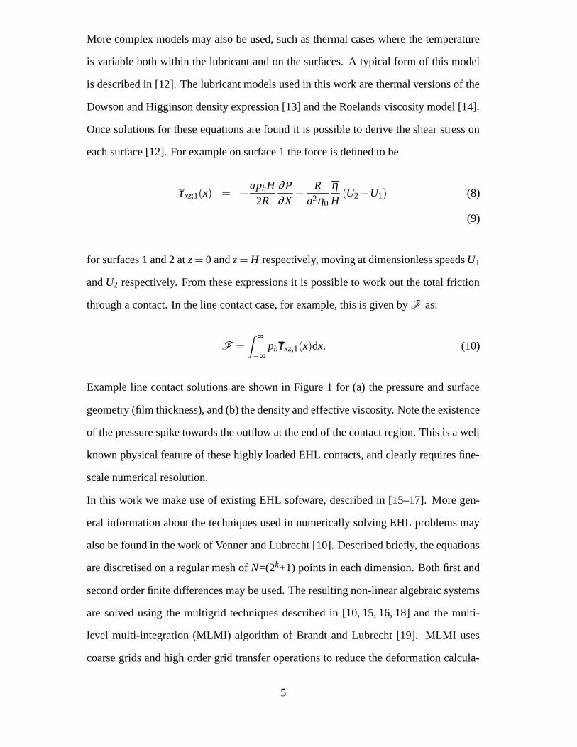
More complex models may also be used, such as thermal cases where the temperature

is variable both within the lubricant and on the surfaces. A typical form of this model

is described in [12]. The lubricant models used in this work are thermal versions of the

Dowson and Higginson density expression [13] and the Roelands viscosity model [14].

Once solutions for these equations are found it is possible to derive the shear stress on

each surface [12]. For example on surface 1 the force is defined to be

τxz;1(x) = −aphH

2R∂P∂X

+R

a2η0

ηH

(U2 −U1) (8)

(9)

for surfaces 1 and 2 at z = 0 and z = H respectively, moving at dimensionless speeds U1

and U2 respectively. From these expressions it is possible to work out the total friction

through a contact. In the line contact case, for example, this is given by F as:

F =∫ ∞

−∞phτxz;1(x)dx. (10)

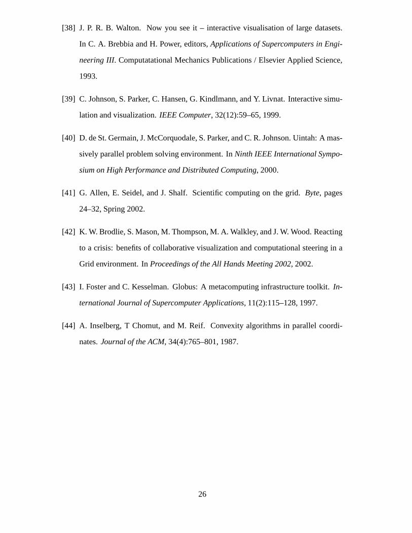
Example line contact solutions are shown in Figure 1 for (a) the pressure and surface

geometry (film thickness), and (b) the density and effective viscosity. Note the existence

of the pressure spike towards the outflow at the end of the contact region. This is a well

known physical feature of these highly loaded EHL contacts, and clearly requires fine-

scale numerical resolution.

In this work we make use of existing EHL software, described in [15–17]. More gen-

eral information about the techniques used in numerically solving EHL problems may

also be found in the work of Venner and Lubrecht [10]. Described briefly, the equations

are discretised on a regular mesh of N=(2k+1) points in each dimension. Both first and

second order finite differences may be used. The resulting non-linear algebraic systems

are solved using the multigrid techniques described in [10, 15, 16, 18] and the multi-

level multi-integration (MLMI) algorithm of Brandt and Lubrecht [19]. MLMI uses

coarse grids and high order grid transfer operations to reduce the deformation calcula-

5

tion (i.e. the integral in (5) from O(N4) to O(N2 lnN2). The single grid cost is so high

since the discrete version of Equation (5) is a multi-summation of the entire fine domain,

for each point. In this work we have used sixth order coarsening to restrict the finer grid

solutions through a hierarchy of grids to the coarsest grid. It is on this coarsest grid that

the multi-summation is performed, at a fraction of the cost. The calculated contribu-

tions to the deformation are then prolonged back through the hierarchy, correcting the

approximation to the summation near each point by having a more accurate summation

in the locale.

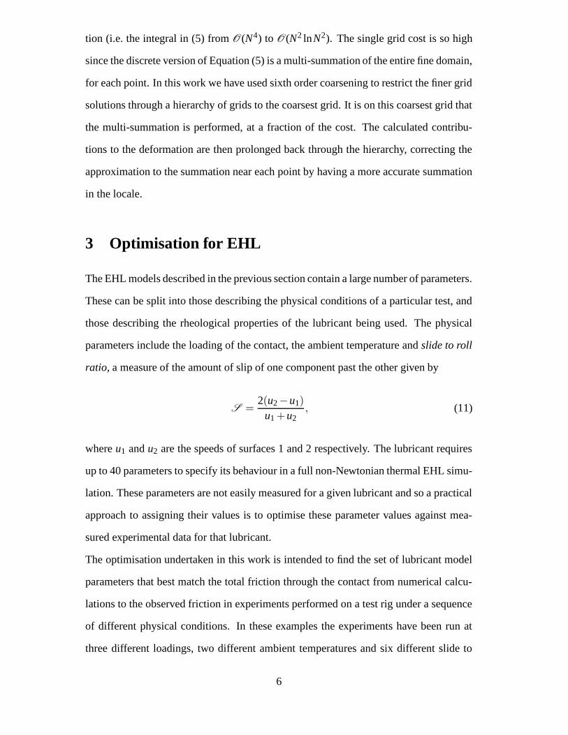
3 Optimisation for EHL

The EHL models described in the previous section contain a large number of parameters.

These can be split into those describing the physical conditions of a particular test, and

those describing the rheological properties of the lubricant being used. The physical

parameters include the loading of the contact, the ambient temperature and slide to roll

ratio, a measure of the amount of slip of one component past the other given by

S =2(u2 −u1)

u1 +u2, (11)

where u1 and u2 are the speeds of surfaces 1 and 2 respectively. The lubricant requires

up to 40 parameters to specify its behaviour in a full non-Newtonian thermal EHL simu-

lation. These parameters are not easily measured for a given lubricant and so a practical

approach to assigning their values is to optimise these parameter values against mea-

sured experimental data for that lubricant.

The optimisation undertaken in this work is intended to find the set of lubricant model

parameters that best match the total friction through the contact from numerical calcu-

lations to the observed friction in experiments performed on a test rig under a sequence

of different physical conditions. In these examples the experiments have been run at

three different loadings, two different ambient temperatures and six different slide to

6

roll ratios, giving a total of 36 different cases, covering a wide range of the operating

conditions which lubricants may undergo in practice. By using a numerical solver it

is possible to run each of these cases for a particular input parameter set. Ten of the

lubricant rheology parameters have been varied to try to find the parameter set that most

closely matches the frictional behaviour of the real lubricant. For a given set of lubricant

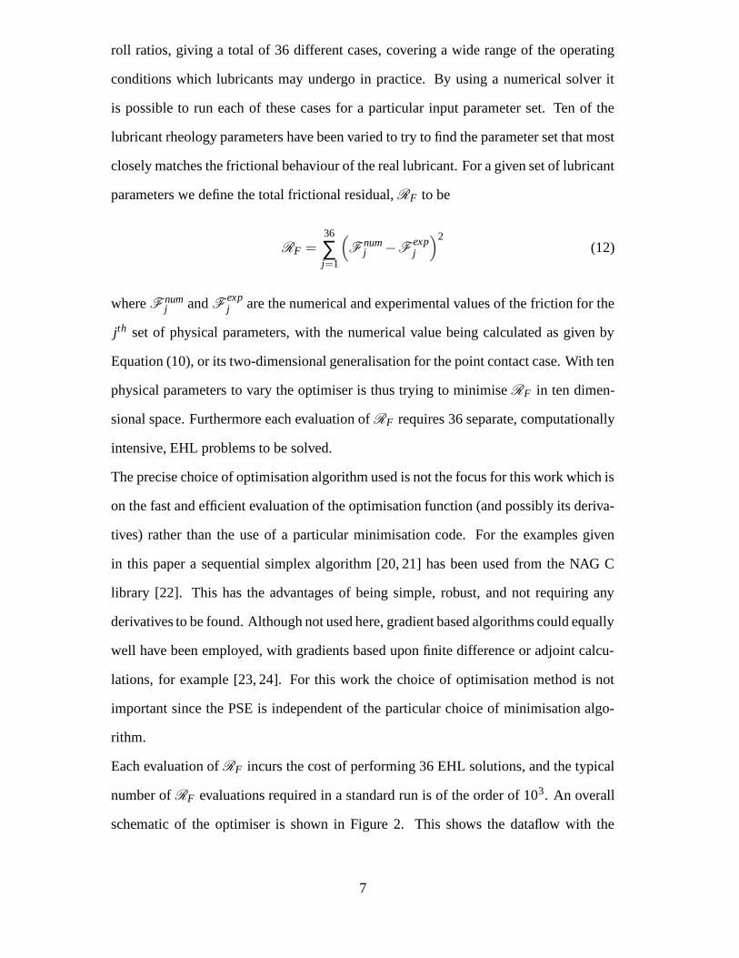
parameters we define the total frictional residual, RF to be

RF =36

∑j=1

(

Fnumj −F

expj

)2(12)

where F numj and F

expj are the numerical and experimental values of the friction for the

jth set of physical parameters, with the numerical value being calculated as given by

Equation (10), or its two-dimensional generalisation for the point contact case. With ten

physical parameters to vary the optimiser is thus trying to minimise RF in ten dimen-

sional space. Furthermore each evaluation of RF requires 36 separate, computationally

intensive, EHL problems to be solved.

The precise choice of optimisation algorithm used is not the focus for this work which is

on the fast and efficient evaluation of the optimisation function (and possibly its deriva-

tives) rather than the use of a particular minimisation code. For the examples given

in this paper a sequential simplex algorithm [20, 21] has been used from the NAG C

library [22]. This has the advantages of being simple, robust, and not requiring any

derivatives to be found. Although not used here, gradient based algorithms could equally

well have been employed, with gradients based upon finite difference or adjoint calcu-

lations, for example [23, 24]. For this work the choice of optimisation method is not

important since the PSE is independent of the particular choice of minimisation algo-

rithm.

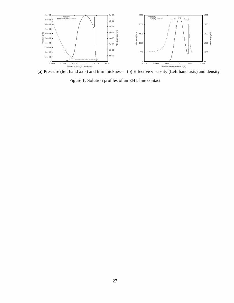
Each evaluation of RF incurs the cost of performing 36 EHL solutions, and the typical

number of RF evaluations required in a standard run is of the order of 103. An overall

schematic of the optimiser is shown in Figure 2. This shows the dataflow with the

7

36 EHL cases at the bottom and different xi, lubricant parameter sets, being supplied

by the optimiser from potential points in the simplex. Each EHL case returns an F j

contribution to the RF value for this particular xi. Finally the optimiser returns a local

minimum solution, xmin, from the search space.

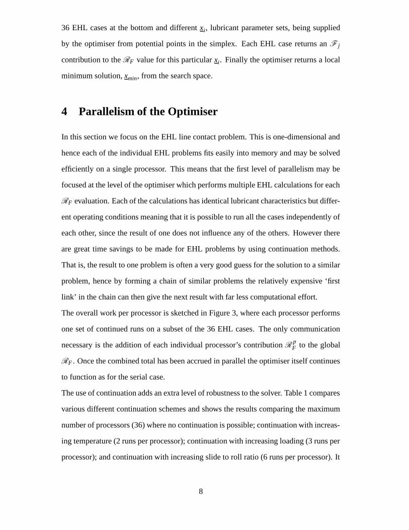
4 Parallelism of the Optimiser

In this section we focus on the EHL line contact problem. This is one-dimensional and

hence each of the individual EHL problems fits easily into memory and may be solved

efficiently on a single processor. This means that the first level of parallelism may be

focused at the level of the optimiser which performs multiple EHL calculations for each

RF evaluation. Each of the calculations has identical lubricant characteristics but differ-

ent operating conditions meaning that it is possible to run all the cases independently of

each other, since the result of one does not influence any of the others. However there

are great time savings to be made for EHL problems by using continuation methods.

That is, the result to one problem is often a very good guess for the solution to a similar

problem, hence by forming a chain of similar problems the relatively expensive ‘first

link’ in the chain can then give the next result with far less computational effort.

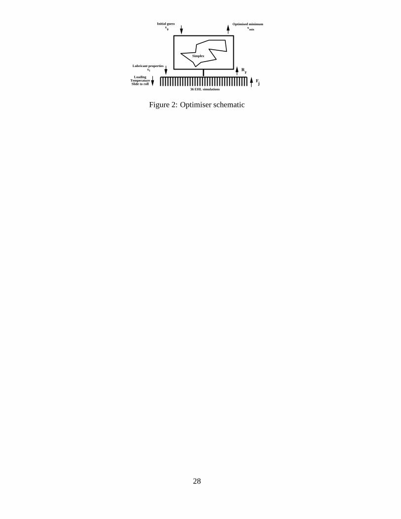
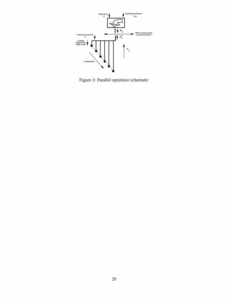
The overall work per processor is sketched in Figure 3, where each processor performs

one set of continued runs on a subset of the 36 EHL cases. The only communication

necessary is the addition of each individual processor’s contribution RpF to the global

RF . Once the combined total has been accrued in parallel the optimiser itself continues

to function as for the serial case.

The use of continuation adds an extra level of robustness to the solver. Table 1 compares

various different continuation schemes and shows the results comparing the maximum

number of processors (36) where no continuation is possible; continuation with increas-

ing temperature (2 runs per processor); continuation with increasing loading (3 runs per

processor); and continuation with increasing slide to roll ratio (6 runs per processor). It

8

can be clearly seen that maximising the amount of continuation used is very important

for increasing the overall efficiency. Where more processors are used continuation be-

tween results is less frequent meaning more full restarts, and hence the parallel speed-up

diminishes. The final line shows the comparative serial code using continuation along

lines of increasing slide-to-roll ratio. The variation in the number of RF evaluations to

reach a local minimum is again due to the lack of continuation since a poor initial guess

can cause the numerical solver not to converge, meaning that the calculated friction is

given a 100% error for that case, therefore affecting the future behaviour of the simplex

algorithm.

The parallel software from this project is designed for computational grids such as the

White Rose Grid [25] with its mixture of shared and distributed memory machines, in-

cluding a 256-processor Beowulf style cluster. For reasons of portability the parallelism

is undertaken using MPI [26].

5 Parallelism of the Solver

The line contact problem discussed in the previous section illustrates how the optimisa-

tion process may be parallelised to increase the solution speed. The same optimisation

process may also be used for 2-d point contact problems however the computational

cost increases still further in this situation. This is overcome through the use of a par-

allel point contact solver, adapted from previous work [7, 27], in order to reduce the

computational time sufficiently to make the optimisation feasible.

5.1 A parallel EHL point contact code

The starting point for the parallelisation of the method described above is the large

amount of work done on parallel multigrid methods [28–31] and work by the authors on

shared memory machines [7]. Discussions as to why parallelisation of multigrid, an al-

ready optimal algorithm, does not readily produce high parallel efficiencies are given by

9

McBryan et al. [30], Llorente et al. [28, 29] and Tuminaro and Womble [31]. The main

problems are the frequency with which coarse grids are encountered, meaning that there

are very high communications costs relative to the computation. This is especially true

once the critical level has been reached, namely the coarse grid where each processor

has the smallest non-trivial amount of computation. The choice left is whether to use

the critical level as the coarsest in the multilevel scheme; to agglomerate, by moving all

the work to a single processor as in Linden et al. [32, 33]; or to have idle processors,

such as used by Brown et al. [34].

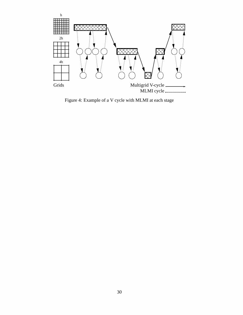
In the case of EHL problems the addition of MLMI causes extra difficulties as even

more work is done at coarse mesh levels. In particular, since no significant computation

is done during the MLMI coarsening the communication costs are already a large factor

in terms of efficiency. A schematic of the overall algorithm is sketched in Figure 4

which shows a multigrid V cycle with multiple MLMI calls at each level. In contrast to

the multigrid method the most striking change is that there is no calculation other than

at the multi-summation and correction stages, all the work is in grid transfer.

The convergence properties of the standard solution methods mean that line solves are

the most efficient multigrid smoothers for these problems [18, 35], and hence such

smoothers have been considered during the parallelisation of the solver. The natural

geometric domain decomposition is therefore that of strips in the direction of the lubri-

cant entrainment. Due to regular grids being used in the solver, it is possible to ensure

that coarser grids are always decomposed onto the same processors as their coincident

finer grid points. This aids communication efficiency during grid transfer. More detailed

discussion of grid transfer is given in [27].

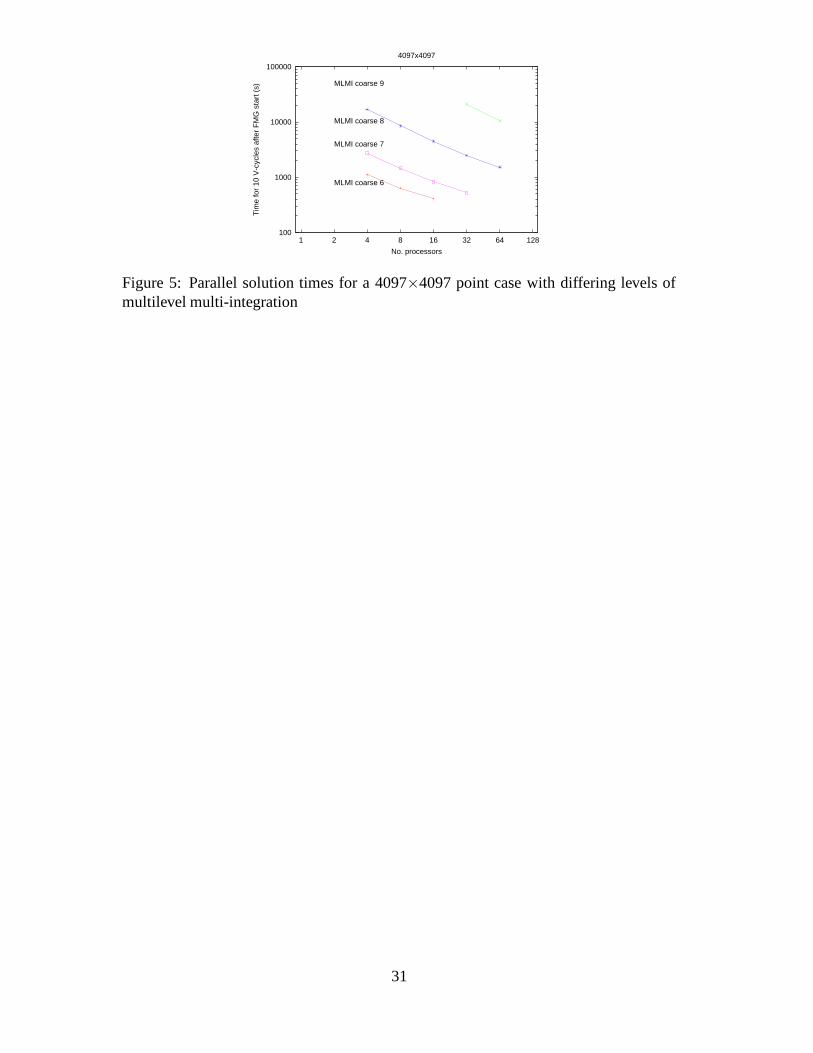
The overall performance of the parallel solver is shown in Figure 5, where the timings

are shown for a typical case on a grid of 4097×4097 points, on up to 64 processors. Note

that as the number of processors increases the size of the coarsest grid increases too, in

order to ensure that the coarsest grid can be partitioned across the processors. This leads

to a loss of efficiency since the deformation calculation (using the MLMI algorithm) is

10

being done more accurately but at a much a higher overall cost. Conversely, if we fix

the size of the coarsest mesh there is a maximum number of processors that may be

used on it. For the cases shown in Figure 5, which is typical in this work, it is clear

that there is little point in going beyond 16 processors on an individual EHL case. A

more comprehensive discussion of these coarse grid issues may be found in [27], and

ways of improving the situation are proposed, although these all add significantly to the

complexity of the implementation.

In this work, however, it is clear from the previous section that additional parallelism is

possible if we make use of a hierarchical approach which combines this parallel solver

with the parallel optimisation described in the previous section. This aims to make

optimal use of the Grid resources available, as outlined in Section 5.2 below, rather

than simply using all the available processors on each single EHL case, which Figure 5

illustrates would be less efficient.

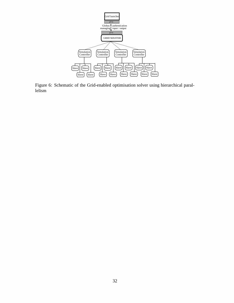
5.2 Hierarchical parallelism

The use of the parallel solver inside the parallel optimiser leads to the notion of hier-

archical parallelism. This is illustrated in Figure 6 where the Grid Master can be seen

to be communicating with a series Simulation Controllers, which, rather than being the

EHL simulations as in the line contact work, are now the lead processes of parallel EHL

simulations.

For reasons of portability the software produced in this work makes use of the MPI li-

brary [26]. In implementing this hierarchical strategy it has been necessary to introduce

additional MPI communication groups, to include local groups for each simulation and a

group for all of the Simulation Controllers. This latter group of processes is responsible

for synchronisation at the end of each RF evaluation, with each Simulation Controller

posting its contribution to RF to the Grid Master. The Grid Master then broadcasts

within this group the necessary information (i.e. the parameter set xi) for the next RF

evaluation. Each Simulation Controller then passes the relevant information down to its

11

worker processes via the local simulation group.

This communication paradigm means that it is possible to take advantage of the Grid,

rather than just traditional HPC technologies. In particular if, rather than a massively

parallel machine, multiple smaller resources are available, then it is possible to use

Globus with Grid-enabled MPI, MPICH-G2 [36], to split the computation sensibly be-

tween resources. This would allow frequent, data-heavy, high speed communication

within single resources for each EHL simulation, but slower speed TCP/IP traffic be-

tween Grid resources transferring small amounts of data only at the end of each contin-

uation series.

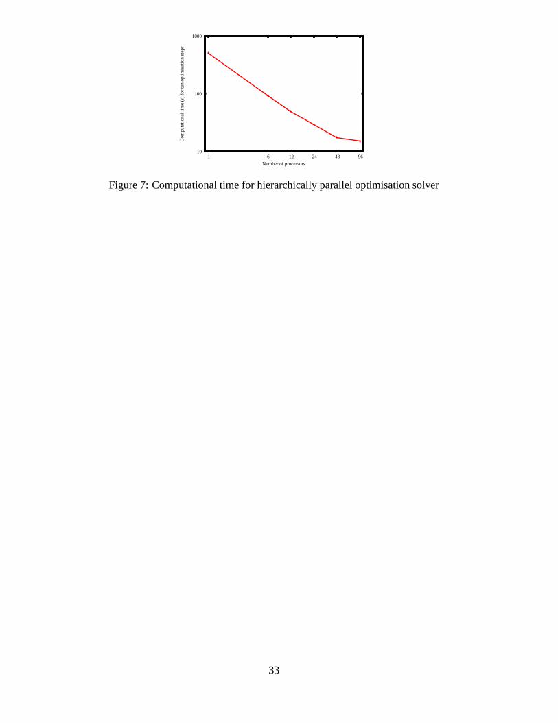
The solution speed for the hierarchical parallelism scheme is illustrated in Figure 7.

This shows the time taken for ten RF evaluations using the hierarchically parallel op-

timisation solver, each EHL solve consisting of ten multigrid V-cycles on a mesh of

1025×1025 points. It may be seen from this figure that the parallelisation of the opti-

miser, with parallelisation of the solver beneath is a good strategy. The issues concerned

with the loss in efficiency beyond 48 processors are three fold. First, the grid resolu-

tion, and hence high level of coarse grid communication is starting to effect the parallel

solution efficiency. The second issue is concerned with the EHL cases not all having

the same computational solution time when the physical parameters are varied. Most

importantly in a Grid setting, however, not all of the 96 processors used in this example

are identical. Hence if one set of parallel computations takes place on a slower set of

processors than the rest this will lead to a loss of overall efficiency. This last observation

raises some interesting issues regarding dynamic load balancing across Grid resources,

however these are beyond the scope of this paper.

6 A Grid-enabled PSE

Problem Solving Environments are a very useful way in which to combine simulation

and visualisation into a single package. The consequential benefit of such a system

12

is that it facilitates experimentation with minimal additional effort from the user. It

is the combination of these elements, combined with the knowledge of the user, that

make such systems potentially very powerful for obtaining understanding of the range

of problems being solved.

PSEs were first proposed by the landmark NSF report of Haber and McNabb [37] and

have become more readily built as software systems, especially visualisation packages,

have evolved. Commercial visualisation packages, such as NAG’s IRIS Explorer [38],

AVS, and IBM’s OpenDX, all have functionality for including simulation components.

Some open source PSEs have also been developed, most notable among them being

SCIRun [39] which has grown out of a more focused PSE for a particular (medical)

application, to become the more general system of its latest releases.

The integration of Grid technology with PSEs is now a natural step in this evolution.

The ideas of ‘workflow’ in Grid terminology correspond very closely with how PSEs

are generally constructed within any of the environments cited above. Besides the PSEs

designed for EHL problems, which are clearly the most relevant to this paper, [6, 7],

there are several other related works of note. A good example of a specific PSE being

extended to massively parallel computers is Uintah [40] which has extended SCIRun

through a common component architecture. Uintah is currently being developed further

using the Globus toolkit, as is the Cactus project [41].

6.1 The gViz libraries

Much of the new Grid-enabling work described in this paper makes use of the gViz

libraries which are described in full in [11]. In brief, gViz provides a communication

interface for a process running on a (typically) Grid resource to enable other users to

connect to the simulation and either visualise the results or steer the calculation. It does

this by providing a library of functions for communication of data between separate

programs.

A schematic for the gViz communications patterns is provided in Figure 8, which shows

13

the main desktop PSE being connected to a remote simulation through channels labelled

‘Grid’, ‘Visualise’ and ‘Steer’. The functions are described in detail in the following

paragraphs. In addition Figure 8 also illustrates a second PSE that is able to connect with

the remote simulation. A connection is indicated between the two PSEs themselves,

representing the fact that some information may be shared at the desktop level, without

involving the remote simulation. Examples of such include camera position, adding

pointers to solution features, or sharing visualisation quantities.

When the simulation is launched from the main PSE it is important for the PSE to know

where to find the simulation, so that it can initiate the necessary connections through

the use of sockets. In the simplest scenario the ‘launcher’ specifies as command line

arguments its machine name and a specific port on which it will be listening. The

simulation then uses this advertised location to return the location of the running threads.

This destination location is kept the same for all new listeners to connect through. This

is referred to in Figure 8 as the ‘Grid’ channel. A more complicated scenario involves

the use of a gViz directory service. If specified at launch time then the simulation will

register here rather than with the desktop PSE. This enables the location of the running

simulation to be advertised in a more persistent manner, thereby aiding other desktop

PSEs wishing to connect for the purposes of collaboration or asynchronous steering.

Once the simulation on the Grid resource is running it must start its own ‘Visualise’ and

‘Steer’ channels. This is done through separate threads which wait until a “listener”

makes a connection. If a connection is made to one of these threads then an additional

thread will start and wait for the next listener. When the connection to a listener is

terminated, the thread is also closed to free the memory and the port. Throughout the

execution of the simulation it is these ‘Steer’ and ‘Visualise’ channels along which data

flows. User requests for computational steering are sent via the ‘Steer’ channel. The

main simulation thread will query the steering thread at suitable intervals to receive any

updates. The steering data is a predefined list of inputs to the simulation and hence this

is usually a relatively short list. Through the gViz functions a user may change one or

14

multiple values at any time. Steering information is synchronised between connected

PSEs so changes made by one user are reflected on the desktop of any others.

Whenever an output dataset is ready it is made available through the ‘Visualise’ channel.

This data is typically far larger in quantity, and less regularly defined, than the steering

data and hence gViz requires the application developer to make available all the in-

formation needed by the desktop PSEs to create a visualisation. Typically this data is

broken down into coherent blocks of similar data, such as coordinates of mesh points,

and solutions values, along with basic variables such as the number of dimensions and

the number of datasets being returned. In order to receive this information the desktop

PSE must allocate memory of the appropriate size and so after receiving the number

of blocks being sent, the simulation will transmit the number of bytes in each block.

The PSE-end of the application can then convert the raw data into native data formats

for the particular PSE being used. Any listeners connecting to the simulation are able

to receive the latest dataset and hence all such information is retained at the simulation

end, rather than on the desktop. Visualisation conversions from gViz to PSE-package

specific formats have been successfully implemented for IRIS Explorer, SCIRun, Mat-

lab and VTK. Note that since raw data is being returned through the ‘Visualise’ channel,

different PSEs may choose to perform very different visualisations at the same time.

6.2 Architecture

An example of a typical IRIS Explorer map for the EHL lubricant parameter optimisa-

tion PSE is shown in Figure 9 where the dataflow pipeline, generally from left to right,

is clearly visible. The majority of the modules are used in the visualisation process and

hence only the three modules on the left are described in the following paragraphs.

The first module in the map shown in Figure 9, GlobusSearch, interrogates a GIIS (Grid

Index Information Service) server to analyse the available resources and their current

statuses [42]. The user can then select a resource and choose a suitable launch method,

including launching the job onto the Grid using Globus [43]. For this work we have ex-

15

tended the gViz library to include parallel launch mechanisms including writing a par-

allel job submission script or a Globus RSL (Resource Specification Language) script

which then gets submitted to Sun Grid Engine for scheduling onto a suitable node.

When the job is launched only one of the parallel processes will initiate the gViz library

and handle the communication between the Grid job and the desktop PSE. The infor-

mation returned to the desktop, described above, detailing the location of the Grid job is

then passed to the next two modules in the map, SteerGOSPEL and VisualiseGOSPEL.

Knowledge of where the simulation is running also allows any other user to access the

simulation through the gViz libraries. This means that one person, with Grid certifica-

tion, can start the simulation and other collaborators around the world can then all see

the results of that simulation and help to steer the computation [8,42]. In fact, the person

who originally launched the Grid job need not actually be involved from that point on.

Computational steering is the ability to change a simulation that is already running. One

example of this could be choosing to use a lower quality mesh in the early stages of the

solve, but as the solution gets near to a local optimum using a higher resolution mesh to

improve the accuracy of the solution obtained. The module SteerGOSPEL has several

uses. Firstly it shows the current best set of values found by the optimisation algorithm,

along with RF . This allows a user access to individual numbers from the simulation

rather than much larger datasets for visualisation purposes. These numbers can also

be used for steering. For example it is possible to resubmit this current best set to the

optimiser once a minimum has been found. The simplex algorithm will then build a new

simplex around this previous minimum, potentially allowing it to escape from local

minima. Similarly, a different point in the search space can be specified away from

regions in which the optimiser has previously searched. Alternatively, as mentioned

above, the accuracy can be changed. A further method that we have implemented in

this work is the ability to change the underlying mathematical model being used. In the

case of EHL simulations, for example, we permit the user to turn on (or off) the thermal

components of the solution. The thermal solve (i.e. treating temperature as a variable

16

across the contact through addition of an energy equation) is much more expensive but

adds greater accuracy to the friction results obtained, especially for those cases where

more heat is generated [15].

Communication from the PSE to the simulation is done, as described above, through

the gViz libraries. At suitable points the simulation will check if any new input data has

been received. If a steering request is for additional accuracy, say, then these changes

can be introduced without changing the points of the current simplex and would there-

fore only apply to future calculations. If, on the other hand, a new simplex was requested

then the use of a communication flag inside the routine will cause the optimisation rou-

tine to terminate and then restart with the new simplex.

The VisualiseGOSPEL module communicates with the simulation to receive all of the

datasets for visualisation. These are then packaged up into standard IRIS Explorer

datatypes and sent down the rest of the map for visualisation. When the full datasets are

being shown then more information needs to be returned from the parallel nodes than is

necessary for just the optimisation process. Descriptions of the most significant output

datasets are provided in the following section.

6.3 Visualisation

A full optimisation run generates very large quantities of high-dimensional multivari-

ate data even though each single EHL simulation is reduced to just one number, F numj ,

from Equation (12). The distance each of these calculated values is away from Fexpj

is one piece of information that may be of interest to a user wishing to steer the op-

timisation. For example if the results were all good except at, say, very high ambient

temperatures then engineering knowledge of which parameters affect the accuracy at

such temperatures could be used to accelerate the optimisation process. A visualisation

of such data is shown in Figure 10 which consists of a 2-d plane with increasing slide

to roll ratios plotted against experimental friction for each of the loadings and ambient

temperatures. The 3-d surface represents the errors in each of the calculated friction

17

values. If a perfect solution was found this would collapse to lie exactly on the six lines

of experimental results.

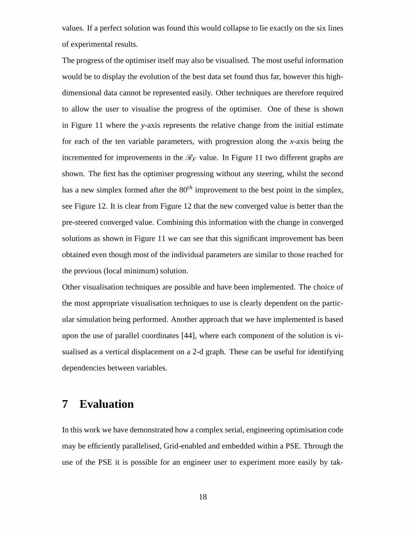
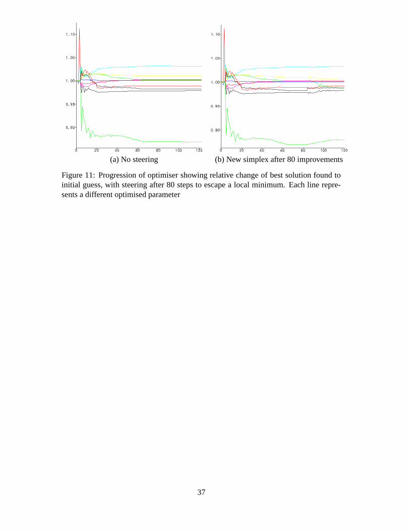
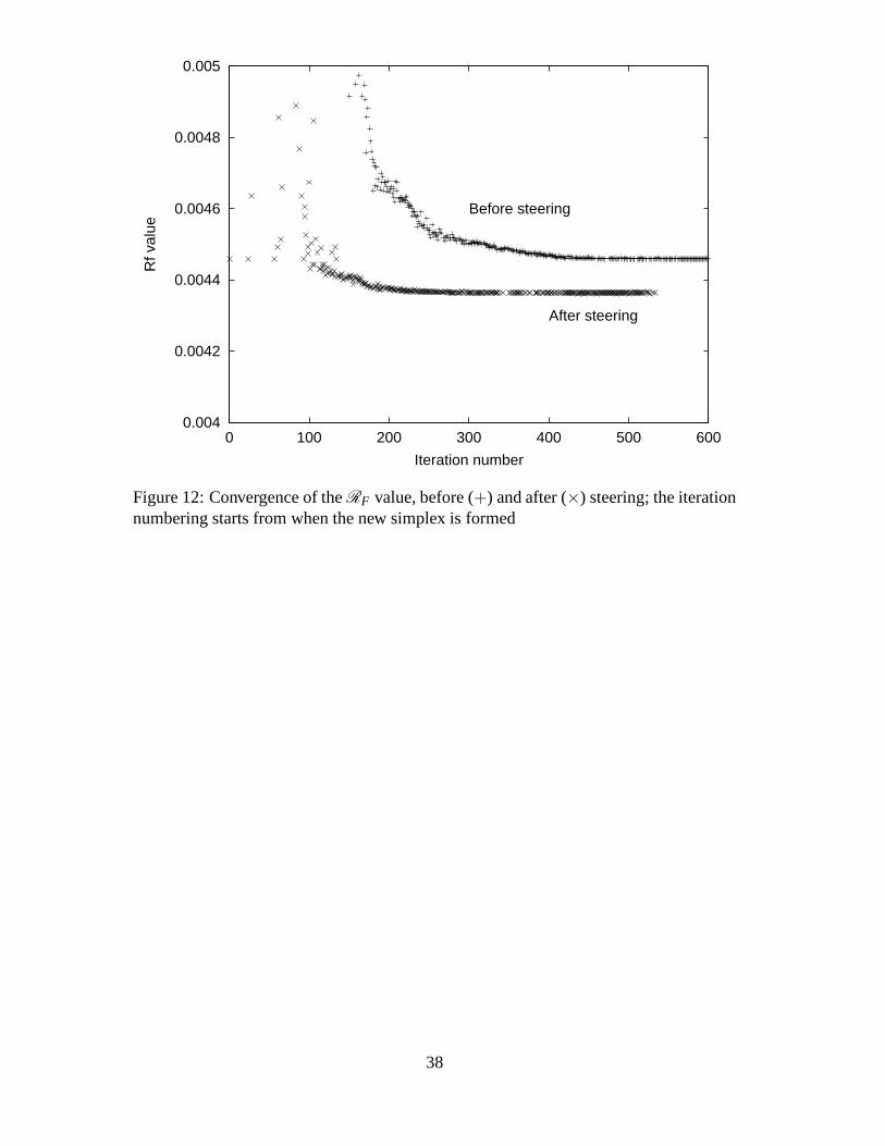
The progress of the optimiser itself may also be visualised. The most useful information

would be to display the evolution of the best data set found thus far, however this high-

dimensional data cannot be represented easily. Other techniques are therefore required

to allow the user to visualise the progress of the optimiser. One of these is shown

in Figure 11 where the y-axis represents the relative change from the initial estimate

for each of the ten variable parameters, with progression along the x-axis being the

incremented for improvements in the RF value. In Figure 11 two different graphs are

shown. The first has the optimiser progressing without any steering, whilst the second

has a new simplex formed after the 80th improvement to the best point in the simplex,

see Figure 12. It is clear from Figure 12 that the new converged value is better than the

pre-steered converged value. Combining this information with the change in converged

solutions as shown in Figure 11 we can see that this significant improvement has been

obtained even though most of the individual parameters are similar to those reached for

the previous (local minimum) solution.

Other visualisation techniques are possible and have been implemented. The choice of

the most appropriate visualisation techniques to use is clearly dependent on the partic-

ular simulation being performed. Another approach that we have implemented is based

upon the use of parallel coordinates [44], where each component of the solution is vi-

sualised as a vertical displacement on a 2-d graph. These can be useful for identifying

dependencies between variables.

7 Evaluation

In this work we have demonstrated how a complex serial, engineering optimisation code

may be efficiently parallelised, Grid-enabled and embedded within a PSE. Through the

use of the PSE it is possible for an engineer user to experiment more easily by tak-

18

ing advantage of the benefits of concurrent simulation and visualisation, and the use

of computational steering. The specific visualisation demands for this particular ap-

plication are driven by the needs of the users, so as to help them to gain insight into

a multidimensional parameter space; enabling them to escape from local minima, as

well as understanding the nature of the EHL simulations being computed. The use of

parallelism in the simulation has decreased the real-time execution of the simulation sig-

nificantly and the hierarchical parallelism approach has facilitated tackling much more

complex optimisation problems than had previously been feasible. The use of MPI for

the parallelism has allowed portability between Grid resources, and use of the open

source gViz libraries has ensured that the communication between different platforms

of PSE and Grid resource is similarly transparent.

In order to transform the PSE demonstrated in this work to a different problem domain

the following issues would need to be considered.

• Inputs – for many real engineering applications there can be large numbers of

input quantities used in the software. These will be a mixture of physical descrip-

tions, numerical parameters for the solver, and perhaps even choices of solution

methods to be used. Deciding which of these to expose to the user will depend on

their level of expertise.

• Steering – it is necessary to decide which of the input quantities to steer based

upon how changes in each of these are likely to affect the progress of the solver.

For instance in our scenario increasing the resolution of the domain is a relatively

minor change compared with switching the oil being tested.

• Outputs – choice of precisely what data to make available for output visualisations

can be non-trivial. In cases such as the optimisation example of this paper, the

large numerical solutions to the individual cases will generally be reduced to just

a few numbers, but these can be combined with other related results to produce

more detailed understanding.

19

• Parallelism – we have demonstrated that the use of hierarchical parallelism can be

highly beneficial. However we have also seen that whenever there are independent

cases being solved results may be strung together in continuation chains to reduce

the degree of parallelism, but increase the overall performance. This issue is

therefore possibly the most problem specific matter that must be considered when

transforming the PSE.

At least two significant generic conclusions may be drawn from this work. The con-

cept of not only running a computationally intensive code on remote Grid resources,

but also of interacting with it in real time, has been demonstrated to be feasible for a

non-trivial engineering test-problem. This has important implications for the ways in

which computational scientists and engineers may work with large-scale off-site com-

pute resources, as well as allowing physically distributed team members to interact with

Grid-based simulations. Furthermore the concept of hierarchical parallelism, in which a

task is partitioned across more than one parallel computational resource on the Grid, has

also been demonstrated to be a powerful practical tool for Grid computing. This partic-

ular research conclusion is of potential significance whenever an ensemble of compu-

tationally intensive calculations are required, not only for optimisation problems of the

type considered here, but also when sensitivity analysis is necessary or when numerical

derivatives are being calculated for example.

One of the main areas for future expansion of these ideas is to undertake additional

research and development into the effective incorporation of data security. The data

used in engineering simulations is often commercially sensitive and so secure methods

of communicating this to and from remote Grid resources must be considered. This

particular work was undertaken using the White Rose Grid [25] which has a number of

standard security devices implemented, but is not designed to have the same levels of

security that one would expect from within a single organisation.

Another area for future expansion concerns more general bookkeeping. When multiple

simulations are running and a new user wants to join in a collaboration, they may need

20

to know more than the name and location of each simulation currently listed in the

directory service. More detailed information such as steering histories and current active

users could be very useful.

The final area of future research that we highlight here is that of dynamic load balancing

on the Grid. As we have seen in this work, when a job is partitioned across more

than one architecture on the Grid it is not necessarily a good load balancing strategy to

assume that all processors have the same performance. It would be helpful to establish

a robust dynamic load balancing strategy that could move work between resources as

and when it identified imbalances in their utilisation.

Acknowledgements

The authors wish to thank the DTI and EPSRC for funding this work with Shell Global

Solutions through Core Programme e-Science grant number GR/S19486/01. Jason

Wood is also gratefully acknowledged for supplying and supporting the gViz library

used in this work.

References

[1] G. C. Fox and W. Furmanski. High performance commodity computing. In I. Fos-

ter and C. Kesselman, editors, The Grid 2: Blueprint for a New Computing Infras-

tructure, pages 237–255. Morgan Kaufmann, 2004.

[2] K. L. Wang and A. J. Baker. A modular collaborative parallel CFD workbench.

Journal of Supercomputing, 22(1):45–53, 2002.

[3] C. R. Johnson, M. Berzins, L. Zhukov, and R. Coffey. SCIRun: Application to

atmospheric dispersion problems using unstructured meshes. In M. J. Baines,

editor, Numerical Methods for Fluid Mechanics VI, pages 111–122. ICFD ’98,

Oxford, 1998.

21

[4] H. Wright, K. W. Brodlie, and T. David. Navigating high-dimensional spaces to

support design steering. In VIS 2000, pages 291–296. IEEE, 2000.

[5] D. Dabdub, K. M. Chandy, and T. T. Hewett. Managing specificity and general-

ity: tailoring general archetypal PSEs to specific users. In E. N. Houstis, J. R.

Rice, E. Gallopoulos, and R. Bramley, editors, Enabling Technologies for Com-

putational Science: Frameworks, Middleware and Environments, pages 65–77.

Kluwer Academic Publishers, Boston / Dordrecht / London, 2000.

[6] C. E. Goodyer and M. Berzins. Eclipse and Ellipse: PSEs for EHL solutions using

IRIS Explorer and SCIRun. In P. M. A. Sloot, C. J. K. Tan, J. J. Dongarra, and

A. G. Hoekstra, editors, Computational Science, ICCS 2002 Part I, Lecture Notes

in Computer Science, volume 2329, pages 521–530. Springer, 2002.

[7] C. E. Goodyer, J. Wood, and M. Berzins. A parallel Grid based PSE for EHL

problems. In J. Fagerholm, J. Haataja, J. Jarvinen, M. Lyly, P. Raback, and

V. Savolainen, editors, Applied Parallel Computing, Proceedings of PARA ’02,

Lecture Notes in Computer Science, volume 2367, pages 523–532. Springer, 2002.

[8] M. A. Walkley, J. Wood, and K. W. Brodlie. A distributed collaborative problem

solving environment. In P. M. A. Sloot, C. J. K. Tan, J. J. Dongarra, and A. G.

Hoekstra, editors, Computational Science, ICCS 2002 Part I, Lecture Notes in

Computer Science, volume 2329, pages 853–861. Springer, 2002.

[9] D. Dowson. Elastohydrodynamic and micro-elastohydrodynamic lubrication.

WEAR, 190:125–138, 1995.

[10] C. H. Venner and A. A. Lubrecht. Multilevel Methods in Lubrication. Elsevier,

2000.

[11] J. W. Wood, K. W. Brodlie, and J. P. R. Walton. gViz: Visualization and com-

putational steering for e-Science. In S. Cox, editor, Proceedings of the All Hands

Meeting 2003, pages 164–171. EPSRC, 2003. ISBN: 1-904425-11-9.

22

[12] L. E. Scales. Quantifying the rheological basis of traction fluid performance.

In Proceedings of the SAE International Fuels and Lubricants Meeting, Toronto,

Canada. Society of Automotive Engineers, 1999.

[13] D. Dowson and G. R. Higginson. Elasto-hydrodynamic Lubrication, The Funda-

mentals of Roller and Gear Lubrication. Permagon Press, Oxford, Great Britain,

1966.

[14] C. J. A. Roelands. Correlational Aspects of the viscosity-temperature-pressure

relationship of lubricating oils. PhD thesis, Technische Hogeschool Delft, The

Netherlands, 1966.

[15] R. Fairlie, C. E. Goodyer, M. Berzins, and L. E. Scales. Numerical modelling of

thermal effects in elastohydrodynamic lubrication solvers. In D. Dowson et al.,

editor, Trobological Research and Design for Engineering Systems, Proceedings

of the 29th Leeds-Lyon Symposium on Tribology, pages 675–683. Elsevier, 2003.

[16] C. E. Goodyer. Adaptive Numerical Methods for Elastohydrodynamic Lubrication.

PhD thesis, University of Leeds, Leeds, England, 2001.

[17] C. E. Goodyer, R. Fairlie, D. E. Hart, M. Berzins, and L. E. Scales. Calculation

of friction in steady-state and transient ehl simulations. In A.A. Lubrecht and

G. Dalmaz, editors, Transient Processes in Tribology: Proceedings of the 30th

Leeds-Lyon Symposium on Tribology. Elsevier, 2004.

[18] C. H. Venner. Multilevel Solution of the EHL Line and Point Contact Problems.

PhD thesis, University of Twente, Endschende, The Netherlands, 1991. ISBN 90-

9003974-0.

[19] A. Brandt and A. A. Lubrecht. Multilevel matrix multiplication and fast solution

of integral equations. Journal of Computational Physics, 90(2):348–370, 1990.

[20] J. A. Nelder and R. Mead. A simplex method for function minimization. Comput-

ing Journal, 7:308–313, 1965.

23

[21] J. M. Parkinson and D. Hutchinson. An investigation into the efficiency of variants

on the simplex method. In F. A. Lootsma, editor, Numerical Methods for Non-

linear Optimization, pages 115–135. Academic Press, 1972.

[22] NAG. C software library.

[23] A. Jameson, L. Martinelli, and N. A. Pierce. Optimum aerodynamics design using

the Navier-Stokes equations. Theoretical Computational Fluid Dynamics, 10:213–

237, 1998.

[24] M. B. Giles and N. A. Pierce. An introductiond to the adjoint approach to design.

Flow, Turbulence and Combustion, 65:393–415, 2000.

[25] P. M. Dew, J. G. Schmidt, M. Thompson, and P. Morris. The White Rose Grid:

practice and experience. In S. Cox, editor, Proceedings of the All Hands Meeting

2003, pages 172–179. EPSRC, 2003. ISBN: 1-904425-11-9.

[26] Message Passing Interface Forum. MPI: A message-passing interface standard.

International Journal of Supercomputer Applications, 8(3/4), 1994.

[27] C. E. Goodyer and M. Berzins. Efficient parallelisation of a multilevel elastohy-

drodynamic lubrication solver. Concurrency, submitted.

[28] I. M. Llorente, M. Prieto-Matıas, and B. Diskin. An efficient parallel multigrid

solver for 3-d convection-dominated problems. Technical Report TR-2000-29,

ICASE, 2000.

[29] M. Llorente, F. Tirado, and L. Vazquez. Some aspects about the scalability of

scientific applications on parallel computers. Parallel Computing, 22:1169–1195,

1996.

[30] O. A. McBryan, P. O. Frederickson, J. Linden, A. Schuller, K. Solchenbach,

K. Stuben, C.-A. Thole, and U. Trottenberg. Multigrid methods on parallel com-

24

puters – a survey of recent developments. Impact of Computing in Science and

Engineering, 3:1–75, 1991.

[31] R. S. Tuminaro and D. E. Womble. Analysis of the multigrid FMV cycle on large-

scale parallel machines. SIAM Journal of Scientific Computation, 14(5):1159–

1173, 1993.

[32] J. Linden, G. Lonsdale, H. Ritzdorf, and A. Schuller. Block-structured multigrid

for the navier-stokes equations: experiences and scalability questions. In Visual-

ization Development Environments 2000 Proceedings, volume Proceedings of the

Conference on Parallel Computational Fluid Dynamics 1992, Amsterdam, 1992.

Elsevier Science Publishers B.V.

[33] J. Linden, G. Lonsdale, H. Ritzdorf, and A. Schuller. Scalability aspects of parallel

multigrid. Future Generation Computer Systems, 10(4):429–449, 1994.

[34] P. N. Brown, R. D. Falgout, and J. E. Jones. Semicoarsening multigrid on dis-

tributed memory machines. SIAM Journal on Scientific Computing, 21(5):1823–

1834, 2000.

[35] E. Nurgat, M. Berzins, and L. E. Scales. Solving EHL problems using iterative,

multigrid and homotopy methods. Trans. ASME, Journal of Tribology, 121(1):28–

34, 1999.

[36] N. Karonis, B. Toonen, and I. Foster. MPICH-G2: A Grid-enabled implementation

of the Message Passing Interface. Journal of Parallel and Distributed Computing,

63(5):551–563, 2003.

[37] R. B. Haber and D. A. McNabb. Visualization idioms : A conceptual model for

scientific visualization systems. In B. Shriver G.M. Nielson and L.J. Rosenblum,

editors, Visualization in Scientific Computing, pages 74–93. IEEE, 1990.

25

[38] J. P. R. B. Walton. Now you see it – interactive visualisation of large datasets.

In C. A. Brebbia and H. Power, editors, Applications of Supercomputers in Engi-

neering III. Computatational Mechanics Publications / Elsevier Applied Science,

1993.

[39] C. Johnson, S. Parker, C. Hansen, G. Kindlmann, and Y. Livnat. Interactive simu-

lation and visualization. IEEE Computer, 32(12):59–65, 1999.

[40] D. de St. Germain, J. McCorquodale, S. Parker, and C. R. Johnson. Uintah: A mas-

sively parallel problem solving environment. In Ninth IEEE International Sympo-

sium on High Performance and Distributed Computing, 2000.

[41] G. Allen, E. Seidel, and J. Shalf. Scientific computing on the grid. Byte, pages

24–32, Spring 2002.

[42] K. W. Brodlie, S. Mason, M. Thompson, M. A. Walkley, and J. W. Wood. Reacting

to a crisis: benefits of collaborative visualization and computational steering in a

Grid environment. In Proceedings of the All Hands Meeting 2002, 2002.

[43] I. Foster and C. Kesselman. Globus: A metacomputing infrastructure toolkit. In-

ternational Journal of Supercomputer Applications, 11(2):115–128, 1997.

[44] A. Inselberg, T Chomut, and M. Reif. Convexity algorithms in parallel coordi-

nates. Journal of the ACM, 34(4):765–801, 1987.

26

0

1e+08

2e+08

3e+08

4e+08

5e+08

6e+08

7e+08

8e+08

9e+08

1e+09

-0.003 -0.002 -0.001 0 0.001 0.0020

1e-05

2e-05

3e-05

4e-05

5e-05

6e-05

7e-05

8e-05

Pre

ssur

e (P

a)

Film

thic

knes

s (m

)

Distance through contact (m)

PressureFilm thickness

0

500

1000

1500

2000

2500

-0.003 -0.002 -0.001 0 0.001 0.002950

1000

1050

1100

1150

1200

Vis

cosi

ty (

Pa

s)

Den

sity

(kg

/m )3

Distance through contact (m)

ViscosityDensity

(a) Pressure (left hand axis) and film thickness (b) Effective viscosity (Left hand axis) and density

Figure 1: Solution profiles of an EHL line contact

27

Initial guessx

Simplex

Lubricant propertiesx

LoadingTemperatureSlide to roll

Optimised minimumx

RF

Fj

i

0 min

36 EHL simulations

Figure 2: Optimiser schematic

28

LoadingTemperatureSlide to roll

Initial guessx

Lubricant propertiesx

Optimised minimumx

Fj

i

0 min

Simplex

RF

p

MPI Communicationto other processors

RF

Continuation

Figure 3: Parallel optimiser schematic

29

���������������������������������������������������������������

������������������������������

���������������

��������������

���������������������������������

h

2h

4h

Grids Multigrid V-cycle -

MLMI cycle

Figure 4: Example of a V cycle with MLMI at each stage

30

100

1000

10000

100000

1 2 4 8 16 32 64 128

Tim

e fo

r 10

V-c

ycle

s af

ter

FM

G s

tart

(s)

No. processors

4097x4097

MLMI coarse 6

MLMI coarse 7

MLMI coarse 8

MLMI coarse 9

Figure 5: Parallel solution times for a 4097×4097 point case with differing levels ofmultilevel multi-integration

31

SimulationController

SimulationController

SimulationController

SimulationController

Grid launcher

Slave Slave

Slave Slave

Slave Slave

Slave Slave

Slave Slave

Slave Slave

Slave Slave

Slave Slave

Globus authentication managing input / output

GRID MASTER

gViz

gViz

Figure 6: Schematic of the Grid-enabled optimisation solver using hierarchical paral-lelism

32

10

100

1000

1 6 12 24 48 96

Com

puta

tiona

l tim

e (s

) fo

r te

n op

timis

atio

n st

eps

Number of processors

Figure 7: Computational time for hierarchically parallel optimisation solver

33

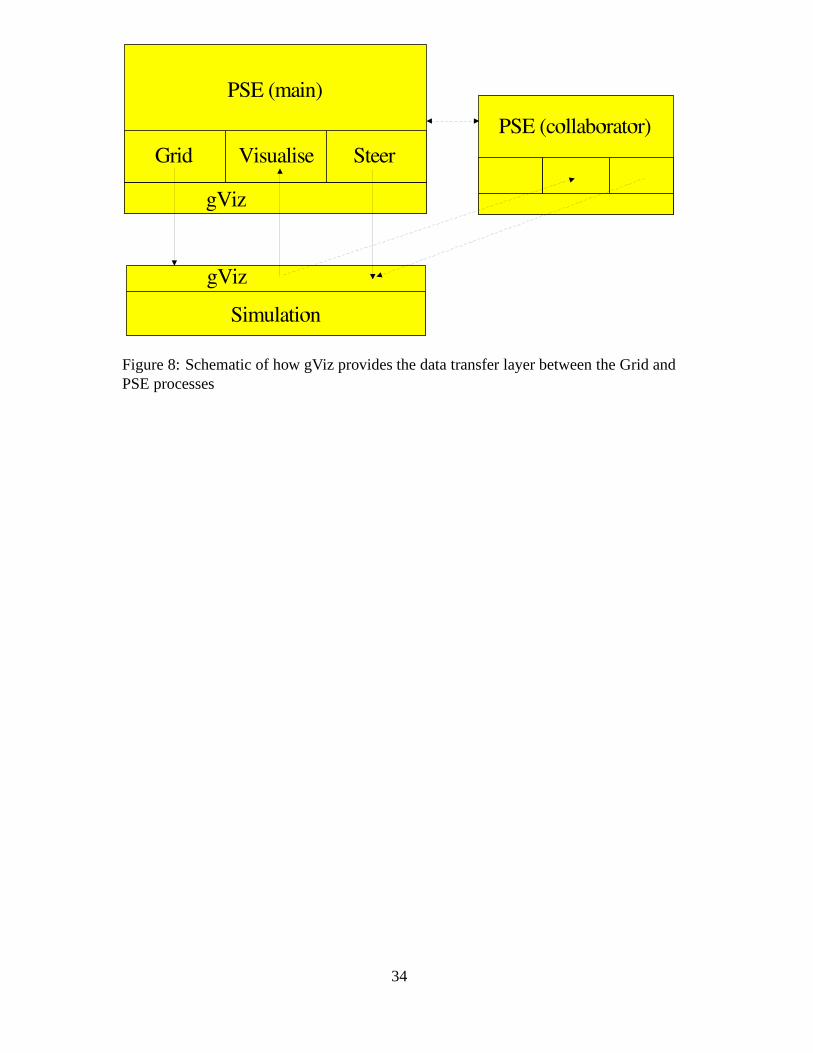
Figure 8: Schematic of how gViz provides the data transfer layer between the Grid andPSE processes

34

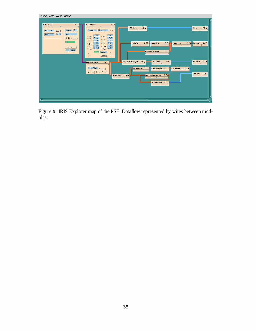
Figure 9: IRIS Explorer map of the PSE. Dataflow represented by wires between mod-ules.

35

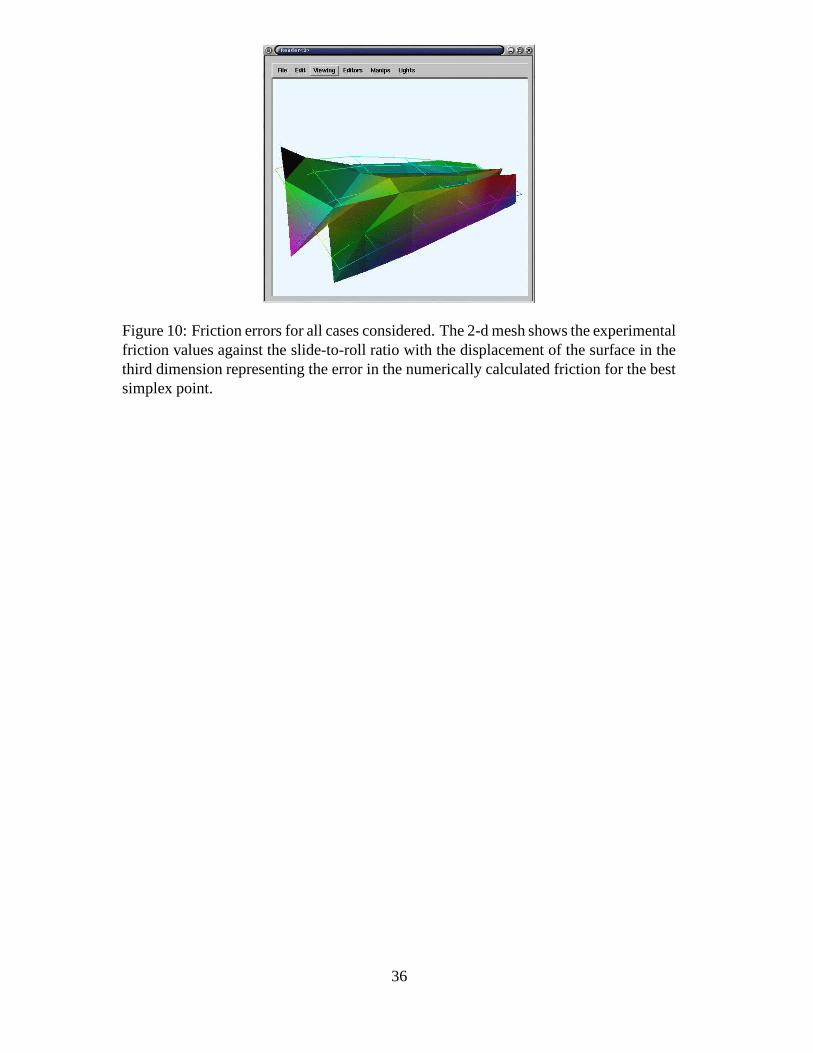
Figure 10: Friction errors for all cases considered. The 2-d mesh shows the experimentalfriction values against the slide-to-roll ratio with the displacement of the surface in thethird dimension representing the error in the numerically calculated friction for the bestsimplex point.

36

(a) No steering (b) New simplex after 80 improvements

Figure 11: Progression of optimiser showing relative change of best solution found toinitial guess, with steering after 80 steps to escape a local minimum. Each line repre-sents a different optimised parameter

37

0.004

0.0042

0.0044

0.0046

0.0048

0.005

0 100 200 300 400 500 600

Rf v

alue

Iteration number

Before steering

After steering

Figure 12: Convergence of the RF value, before (+) and after (×) steering; the iterationnumbering starts from when the new simplex is formed

38

Continuationscheme

ProcessorsSolutiontime (s)

Number of RF

evaluations

Average timeper RF

evaluation (s)No continuation 36 2062 1009 2.04

Temperature 18 559 254 2.20Loading 12 341 163 2.09

Slide to roll 6 531 217 2.45Slide to roll 1 2560 217 11.80

Table 1: Optimiser solution times for varying continuation schemes

39