A GRASP algorithm for fast hybrid high-dimensional datasets

A GRASP algorithm for fast hybrid1

(filter-wrapper) feature subset selection in2

high-dimensional datasets3

Pablo Bermejo, Jose A. Gamez, Jose M. Puerta4

{Pablo.Bermejo,Jose.Gamez,Jose.Puerta}@uclm.es5

Intelligent Systems and Data Mining Laboratory. Computing Systems Department6

Universidad de Castilla-La Mancha. Albacete, 02071, Spain7

Abstract8

Feature subset selection is a key problem in the data-mining classification task

that helps to obtain more compact and understandable models without degrad-

ing (or even improving) their performance. In this work we focus on FSS in

high-dimensional datasets, that is, with a very large number of predictive at-

tributes. In this case, standard sophisticated wrapper algorithms cannot be

applied because of their complexity, and computationally lighter filter-wrapper

algorithms have recently been proposed. In this work we propose a stochastic al-

gorithm based on the GRASP meta-heuristic, with the main goal of speeding up

the feature subset selection process, basically by reducing the number of wrap-

per evaluations to carry out. GRASP is a multi-start constructive method which

constructs a solution in its first stage, and then runs an improving stage over that

solution. Several instances of the proposed GRASP method are experimentally

tested and compared with state-of-the-art algorithms over 12 high-dimensional

datasets. The statistical analysis of the results shows that our proposal is com-

parable in accuracy and cardinality of the selected subset to previous algorithms,

but requires significantly fewer evaluations.

Keywords: Feature selection, classification, GRASP, filter, wrapper,9

high-dimensional datasets10

Preprint submitted to Elsevier February 9, 2011

1. Introduction11

This paper deals with the problem of Feature Subset Selection (FSS) in12

the task of supervised classification. Supervised classification is probably the13

data-mining / machine-learning technique that is most commonly used in prac-14

tice. The goal is to learn a function or classifier C from a training set that15

consists of pairs (−→x , c), where −→x = (x1, . . . , xn) denotes the value assigned16

for each attribute in this instance, and y is its correct output. Variables in17

X = {X1, . . . , Xn} are known as predictive attributes while C is known as the18

class, and it can take a finite number {c1, . . . , ck} of values/states/categories or19

simply classes. Thus, we aim to learn a function C : X1 × · · · ×Xn → C that is20

able to generalize from the known data presented in the training set to unseen21

situations in a reasonable way.22

In the data-mining / machine learning community the function C is referred23

to as a classifier and can belong to different paradigms: decision trees (Quinlan,24

1986), Bayesian classifiers (Duda and Hart, 1973; Webb et al., 2005), nearest25

neighbours (Aha et al., 1991), neural networks (Bishop, 1995), support vector26

machines (Boser et al., 1992), etc. In all cases, the time needed to learn and27

execute the classifier, as well as its complexity and the probability of over-fitting,28

increases when we have a large number of predictive attributes, many of them29

being irrelevant or redundant in the presence of others. Because of these reasons,30

and others such as the cost (not only economic) associated with each predictive31

attribute (e.g. physical sensors, medical tests, invasive surgery, etc), reducing32

the number of predictive attributes but without degrading the performance of33

the classifier is one of the data preprocessing tasks most frequently dealt with34

in the literature. This task receives the name of feature subset selection (FSS)35

or variable selection (Guyon and Elisseeff, 2003; Liu and Motoda, 1998) and its36

2

performance can be meassured in different ways, the most commonly used being37

the accuracy of the classifier obtained.38

In this paper we focus on the framework described above (supervised clas-39

sification and the use of accuracy as performance measure), but in addition40

we add the constraint of dealing with high-dimensional datasets, that is, we41

are interested in carrying out FSS over datasets having thousands of variables42

(microarrays, text-mining, etc.). Our goal is to develop an algorithm able to per-43

form FSS efficiently in high-dimensional datasets, and so we aim to maintain (or44

improve) the performance (accuracy and compactness) of previous approaches45

in the literature for dealing with this type of datasets (sequential and incremen-46

tal FSS algorithms (Ruiz et al., 2006; Bermejo et al., 2009; Kittler, 1978)) whilst47

carrying out a significantly smaller number of evaluations. To do this, we pro-48

pose to hybridize these types of FSS algorithms with a randomized algorithm49

known as GRASP (Greedy Randomized Adaptive Search Procedure) (Feo and50

Resende, 1995). GRASP is a multi-start two-stage algorithm. At each iteration51

the method carries out two steps: first a randomized procedure is used to con-52

struct a potential solution to the problem under study; and then, this solution53

is improved by using (usually) a local search method. Randomization of the54

constructive procedure is needed in order to obtain good but different starting55

points. GRASP can then be viewed as a global optimization method, which56

usually improves the quality of the solution obtained by specific heuristics. As57

we have stated above, our goal in this paper is to take advantage of the degrees58

of freedom provided by GRASP criteria design in order to drastically decrease59

the number of wrapper evaluations (proportional to the CPU time needed), but60

of course, without degrading the performance (classification accuracy).61

Our study is structured as follows: the next section presents some prelim-62

inaries on the FSS problem, while Section 3 introduces the basic description63

3

of GRASP meta-heuristics; Section 4 describes in detail the incremental FSS64

algorithm which is used as a building block in our proposal; then, in Section 565

we present our proposed GRASP-based FSS algorithm and in Section 6 we test66

it by means of a set of experiments over high-dimensional datasets; finally, in67

Section 7 we present our concluding remarks and some ideas for future work.68

2. Feature subset selection69

The goal of FSS is to obtain an (almost) optimal subset of the available70

predictive attributes according to a performance score, classification accuracy71

in our case. Because of the large cardinality (2n) of the search space (P(X)),72

exhaustive search is intractable even for moderate values of n, and so different73

strategies must be employed.74

FSS algorithms result from the combination of (1) a search method and75

(2) an evaluation strategy to score the goodness of the candidate features. By76

excluding Embedded methods, where it is the same algorithm for learning the77

classifier that carries out the FSS process (e.g. C4.5 (Quinlan, 1986)), we can78

identify the following search strategies: Complete, Ranker, Sequential, Incre-79

mental and Metaheuristics. As for the features, these may be evaluated in a80

filter or wrapper way.81

In the filter approach, the goodness of an attribute or set of attributes is82

estimated by using only intrinsic properties of the data, while in the wrapper83

approach, the merit of a given candidate subset is obtained by learning and84

evaluating a classifier using only the variables included in the proposed subset.85

Once candidate subsets can be scored (by using a filter or wrapper), then86

we can use a large number of search strategies in order to look for an (almost)87

optimal subset. In practice, the following strategies are used:88

• Rankers. Variables are ordered by their individual merit with respect89

4

to the class and the first k are selected. This approach is fast because90

evaluations are simple (univariate) and only n evaluations are required.91

The problem is that no interactions between the variables are taken into92

account and so the result is far from optimal. Also, the selection of the93

value for k is a problem in itself.94

• Sequential. In this approach variables are added (or deleted) one by95

one. The most commonly used approaches are sequential forward selection96

(SFS) and sequential backward selection (SBS) (Kittler, 1978), usually in97

combination with a wrapper evaluator. Both algorithms haveO(n2) worst-98

case complexity, but specially in high-dimensional datasets only SFS is99

used because the evaluations are simpler (fewer variables in the selected100

subset).101

• Metaheuristics. Local and specially global metaheuristics algorithms have102

been used for feature subset selection, e.g. tabu search, evolutionary and103

memetic algorithms (Yang and Honavar, 1998; Inza et al., 2000; Casado-104

Yusta, 2009). As they organize the search in a global manner they usually105

obtain better subsets than the previous strategies, but their computational106

cost makes their use (almost) prohibitive in high-dimensional datasets.107

To our knowledge, this type of algorithms have been applied to some108

microarray datasets (2000-7000 variables) in Blanco et al. (2001), but109

using SFS as an initial step to seed the population. In this study, our110

proposal is to obtain an accurate FSS method requiring few evaluations111

with respect to worst-case quadratic approaches, so we cannot assume the112

use of SFS as an initial step.113

• Incremental. This kind of algorithms is relatively recent and although they114

are also sequential in the sense that variables are added one at a time, the115

behaviour is quite different to SFS or SBS. Thus, at each step, instead of116

5

evaluating O(n) candidate subsets, only 1 (or O(|S|)) candidate subsets117

are evaluated. To do this, a rank is firstly computed for the predictive118

attributes by using a filter measure, and then the algorithm visits the119

variables following the ranking and tries to add (Ruiz et al., 2006; Flores120

et al., 2008) replace (Bermejo et al., 2009) the one being studied to/in121

the candidate subset. The advantage of these methods is that they reduce122

the number of wrapper evaluations while maintaining the accuracy of the123

selected subset, so they are more suitable than previous ones for high-124

dimensional datasets.125

3. Preliminaries on GRASP126

We divide this section into two different parts: first, we introduce the basic127

scheme for GRASP, and then we briefly review some applications of GRASP to128

the FSS problem.129

3.1. Greedy Randomized Adaptive Search Procedure (GRASP)130

The greedy randomized adaptive search procedure (GRASP) is a meta-131

heuristic algorithm commonly applied to combinatorial optimization problems.132

Seminal papers for GRASP are (Feo and Resende, 1989, 1995) while new ad-133

vancements and applications can be found for example in (Resende and Ribeiro,134

2010; Festa and Resende, 2010). There are two clear stages in a GRASP algo-135

rithm:136

1. Construction phase. In this step a specific (deterministic) heuristic for137

solving the target problem is taken as a basis for constructing a solution.138

Thus, starting from the empty set, the algorithm adds elements from all139

the possible candidates until a solution is obtained. However, in GRASP140

some randomness is introduced in this step in order to obtain a greedy141

6

randomized construction method (also known as semi-greedy heuristic).142

Thus, instead of choosing the best element at each step of the construction,143

the algorithm chooses at random from a list of promising ones.144

2. Improving phase. The solution constructed is taken as the starting point145

for a local search in order to get an improved solution.146

GRASP algorithms run the previous two phases a number of times, working147

in this way as a multi-start method. Because of the quality provided to the148

solution by the deterministic greedy heuristic used as a basis, and because of149

the variability introduced by the randomness added to the process, we can150

expect to obtain good starting points but with enough variability, and so the151

multi-start method will eventually find a global optimum.152

3.2. Tackling the FSS problem by using GRASP153

Recently, Casado-Yusta (2009) proposed the use of GRASP for feature se-154

lection and compared it with sequential floating algorithms (SFFS, SBFS (Pudil155

et al., 1994)) and other meta-heuristics such as tabu search, genetic algorithms156

and memetic algorithms. Her conclusion is that tabu search and GRASP out-157

perform the other tested methods. The GRASP algorithm follows the canonical158

design shown above, and bases the constructive phase on the randomized se-159

lection of d attributes according to their in-group variability (a filter measure).160

This process is repeated several times and the subset with the best fitness (com-161

puted by using the nearest neighbour approach) is passed as the starting point162

for the improving step, which is carried out by means of a standard hill-climbing163

algorithm that uses the same fitness measure and that also looks for subsets hav-164

ing exactly d variables. Then, the previous steps are iterated a number of times.165

This approach, though returning good results for GRASP with respect to other166

techniques, is not suitable when dealing with high-dimensional datasets. First,167

as we will see in the experiments, there is a great variability in the number of168

7

variables selected for each dataset, so we cannot fix a number a priori. And sec-169

ond, the number of evaluations (tested candidate subsets) with respect to the170

number of variables is too high to be used with tens of thousands of variables.171

In fact, the experiments in Casado-Yusta (2009) only consider datasets having172

between 18 and 57 variables.173

Based on the idea of Casado-Yusta (2009), Esseghir (2010) has devised a new174

proposal for GRASP-based FSS that uses well-known filter algorithms such as175

Relief (Kira and Rendell, 1992) and FCBF (Yu and Liu, 2003) for the construc-176

tive phase, and also classical wrapper FSS algorithms in the improving step.177

This approach is closer to the one presented here because of the hybridization178

of the filter and wrapper methods. However, the use of standard techniques179

in both phases of GRASP makes the resulting algorithm prohibitive for its use180

in high-dimensional datasets. In fact, the experiments carried out by Esseghir181

(2010) only have 34, 57, 60, 69 and 279 attributes, which is far from the goal of182

this paper.183

Apart from FSS, GRASP has been applied to different data-mining prob-184

lems, such as clustering (Cano et al., 2002) and Bayesian networks learning185

(de Campos et al., 2002).186

4. Incremental Wrapper Subset Selection187

Our proposal is largely based on the use of the Incremental Wrapper Subset188

Selection (IWSS) algorithm (Ruiz et al., 2006; Flores et al., 2008), so we describe189

it before explaining our GRASP-based proposal in the next section.190

The IWSS approach (Ruiz et al., 2006; Flores et al., 2008) works in two191

steps:192

• Filter. It evaluates each variable independently with respect to the class193

8

in order to create a ranking. Symmetrical Uncertainty194

SU(Xi, C) = 2

(

H(C)−H(C|Xi)

H(C) +H(Xi)

)

,

is usually considered, where H() denotes Shannon entropy. Variables are195

then ranked from the highest (best) value to the smallest (worst) one.196

• Wrapper. The selected subset S is initialized with the first variable in the197

ranking, and then the algorithm iteratively tries to include in S the next198

variable Xi in the ranking by evaluating the goodness of that augmented199

subset Saux = S ∪ {Xi}. Evaluation of candidate subsets is done in a200

wrapper way, and if a positive difference is obtained, then Xi is added to201

S and discarded otherwise.202

Example 1. Let us assume a problem with eight predictive attributesX1, . . . , X8.203

Assume also that the following values are computed in the filter step: SU(X1, C) =204

0.9, SU(X2, C) = 0.8, SU(X3, C) = 0.6, SU(X4, C) = 0.5, SU(X5, C) = 0.4, SU(X6, C) =205

0.2, SU(X7, C) = 0.1 and SU(X8, C) = 0.01. Therefore the filter ranking is206

r = X1, X2, . . . , X8. Then, the execution of the wrapper phase is:207

tested tested classifier resulting

step variable subset accuracy decision subset

1 X1 {X1} 0.6 accept |S| = {X1}

2 X2 {X1, X2} 0.7 accept |S| = {X1, X2}

3 X3 {X1, X2, X3} 0.68 reject |S| = {X1, X2}

4 X4 {X1, X2, X4} 0.71 accept |S| = {X1, X2, X4}

5 X5 {X1, X2, X4, X5} 0.71 reject |S| = {X1, X2, X4}

6 X6 {X1, X2, X4, X6} 0.65 reject |S| = {X1, X2, X4}

7 X7 {X1, X2, X4, X7} 0.70 reject |S| = {X1, X2, X4}

8 X8 {X1, X2, X4, X8} 0.75 accept |S| = {X1, X2, X4, X8}

208

209

9

and so, |S| = {X1, X2, X4, X8} is the selected subset.210

�211

With the goal of obtaining more compact subsets and of avoiding overfit-212

ting, in Ruiz et al. (2006) wrapper evaluation is carried out by using a 5-fold213

cross validation, and a t-test (confidence level α = 0.1) that takes as input the214

classification accuracy over the five folds to decide when the inclusion of a new215

variable in S is significant. Of course, the same five folds are used in all the216

wrapper evaluations in order to have fair comparisons. This and other criteria217

were studied in Bermejo et al. (2008), concluding that an appropiate method218

is to use a purely heuristic criterion that pursues the same goals: the inclu-219

sion of a variable is significant if the averaged classification accuracy over the220

5 folds is greater than the current one, with this advantage also holding in k221

of the 5 folds (k = 2 and k = 3 are the values recommended in Bermejo et al.222

(2008)). Therefore, now, the decision of acceptance or rejection of the studied223

variable is not based on a comparison between two numbers (as in Example 1)224

acc(S1) > acc(S2) but between two vectors −→acc(S1) ⊲−→acc(S2), where acc(S) is225

the accuracy of the classifier trained using only S as predictive attributes, and226

−→acc(S) is a vector containing the five accuracies corresponding to five-fold cross227

validation carried out using only S as predictive attributes.228

More formally, the relevance criterion used in this paper (⊲) is defined as229

10

follows:230

−→acc(S1) ⊲−→acc(S2) =

true iff

average(−→acc(S1)) > average(−→acc(S2))

and

count(−→acc(S1)[i] >−→acc(S2)[i]) ≥ k

false otherwise

(1)

Example 2. Let us consider −→acc(S1) = [0.7, 0.72, 0.75, 0.73, 0.69] and −→acc(S2) =231

[0.7, 0.71, 0.72, 0.74, 0.69], then −→acc(S1) ⊲−→acc(S2) is true if k = 2 and false if232

k = 3 because average(−→acc(S1)) = 0.718 > average(−→acc(S1)) = 0.712 and233

count(−→acc(S1)[i] >−→acc(S2)[i]) = 2. However, if we have−→acc(S1) = [0.75, 0.7, 0.7, 0.7, 0.7]234

and−→acc(S2) = [0.7, 0.7, 0.7, 0.7, 0.7] then−→acc(S1)⊲−→acc(S2) is false because average(

−→acc(S1)) >235

average(−→acc(S1)) due to only one of the five folds, and so we can consider that236

this success is due to noise or randomness in the partition.237

�238

The IWSS algorithm is very efficient, and linear in the number of attributes,239

O(n), because it carries out exactly n filter and wrapper evaluations. However,240

it also presents two main disadvantages: (1) it relies on a univariate ranking, so241

some interesting variables can be judged irrelevant/relevant just because some242

others have been judged irrelevant/relevant before; and (2) to be sure all the243

potentially relevant variables have been analyzed, the full ranking must be ex-244

plored. As an example, let us observe Figure 1, where we have plotted, for245

the twelve datasets used in our experiments, the relation between the number246

of variables in the datasets and the position in the SU-based ranking of the247

last variable selected by IWSS. As we can observe, in 8 out of the 12 datasets,248

variables after position 100 (the threshold commonly used by the linear-forward249

algorithm (Gutlein et al., 2009)) are selected, while the same happens in 6 out250

11

of the 12 datasets if we consider the first 10% of the ranking as theshold.251

1

10

100

1000

10000

100000

1 10 100 1000 10000 100000

Pos

ition

in r

anki

ng o

f the

last

sel

ecte

d at

trib

ute

Number of attributes in the dataset

Figure 1: Relation between the number of attributes in the dataset and the position of thelast attribute selected by IWSS.

Disadvantage (1) can be alleviated by using other algorithms that follow the252

incremental behaviour but somehow manage in possible interactions between253

the variables (IWSSr (Bermejo et al., 2009), BARS (Ruiz et al., 2009) and254

SFS (Kittler, 1978)). However, these improved incremental algorithms are more255

complex, with O(n2) worst case complexity (or even worse in the case of BARS),256

though in practice this complexity reduces to a sub-quadratic number of wrapper257

evaluations. Therefore, different approaches are needed to deal with datasets258

having a very large number of attributes.259

5. A GRASP algorithm for FSS in high-dimmensional datasets260

In this section we describe a proposal for the GRASP algorithm that re-261

duces the number of evaluations to be sub-linear with respect to the number of262

attributes (n = |X|) and so it is suitable for solving FSS in high-dimensional263

datasets. We start by discussing the idea or intuition behind the proposed264

algorithm and then provide a detailed description.265

12

5.1. The idea266

As mentioned above, our idea is similar to the one simultaneously proposed267

by Esseghir (2010), that is to use a fast algorithm in the constructive step and a268

more sophisticated one in the improving step. However, given the focus of this269

paper, which deals with datasets having a (very) large number of predictive at-270

tributes, the use of standard filter (wrapper) FSS algorithms in the constructive271

(improving) step is not suitable. Notice that our goal is to drastically reduce272

the number of (wrapper) evaluations carried out, so the straightforward use of273

these standard algorithms several times is not a solution.274

What we propose in this study is to use a standard hybrid algorithm (IWSS)275

for the first phase, but to run it over a small subset of the available variables.276

The subset used in each iteration of the constructive phase is sampled by using277

problem-specific knowledge, specifically by using proportional selection based278

on a (noisy) filter score, e.g. SU(Xi, C) + ǫ, where ǫ is a tiny positive number.279

In this way, more promising variables receive more chance of being selected, but280

even variables marginally independent of C will receive a small chance, because281

they can become (conditionally) relevant given some other variable.282

Regarding the improving step, we also need to reduce the number of available283

variables in this phase. Notice that if, as usual, we start from the solution284

returned by the constructive step, S, and try to improve it by using a local285

search procedure (e.g. hill climbing) that has at its disposal all the n predictive286

attributes, then the requirements of such a local optimizer are too high (exactly287

n wrapper evaluations for each hill climbing step). Therefore, we must think of288

a different way of improving.289

Our idea tackles the problem of the comparison of two different solutions.290

When using incremental FSS algorithms this comparison is easy, because we291

operate in a local way. That is, we need to compare a subset S with S ∪292

13

{Xi}. Then, as the goal of FSS is to reduce the number of variables used while293

maintaining or improving the expected accuracy, the inclusion of Xi only makes294

sense if the accuracy of S ∪ {Xi} is better (using ⊲ criterion, eq. 1) than the295

one of only using S. However, when moving to global search, as it is the case of296

GRASP, we need to compare solutions coming from non-adjacent points in the297

search space, which means setting up the comparison not only by accuracy but298

also by subset cardinality. Therefore, we can tackle the problem as a bi-objective299

one and give the following definition:300

Definition 1. Given two candidate subsets S1 and S2, we say that S1 dominates301

S2 if |S1| ≤ |S2| and −→acc(S1) ⊲−→acc(S2). Otherwise we say that S2 is non-302

dominated by S1.303

Example 3. Let us consider two different solutions sol1 = 〈{X1, X2}, 0.9, (f11 , . . . , f

15 )〉304

and sol2 = 〈{X1, X3, X4}, 0.92, (f21 , . . . , f

25 )〉, where the first component is the305

subset of selected variables, the second one is the average accuracy over the306

five folders, and fji is the accuracy in folder i for solution j. Then, which one307

is better?. Perhaps the correct answer depends on some context, but without308

extra information, neither sol1 dominates sol2 nor does sol2 dominate sol1, so309

it is difficult to decide.310

�311

In our proposal we will maintain a set of non-dominated solutions (NDS)312

found during each search performed in the constructive phase. Thus, each time313

a new solution is provided by the constructive step, we will update NDS by314

using it (function update in Figure 2). Since we can expect solutions inside NDS315

to be of good quality, we make a pool with all the variables contained in the316

non-dominated solutions: Xnds, and the local search used in the constructive317

step will be limited to the use of only variables contained in this set, which318

presents a much lower cardinality than the original set of variables. In this way319

14

we expect to perform very fast local search in the improving step, and also to320

perform well because of the quality of the available variables.321

In NDS: the set of non-dominated solutions.sol: the candidate solution to be studied.

Out true if NDS is modified, false otherwiseparameter NDS is modified

1 If sol is dominated by any solution s ∈ NDS then return false

2 else

3 delete from NDS all solutions dominated by sol4 include sol in NDS5 return true

Figure 2: Auxiliary function update(NDS,sol).

5.2. The algorithm322

The pseudo-code of the proposed algorithm is shown in Figure 3. The next323

three subsections describe it in detail.324

5.2.1. Initialization325

Lines 1-5 account for the initialization part of the algorithm. Specifically, we326

initialize the set of non-dominated solutions (NDS) to be empty, and compute327

the marginal filter score for each variable with respect to the class in lines 2 and328

3. We store the results in scores[] in order to avoid having to re-compute them329

each time a filter score is needed (constructive step). In this study MT(Xi, C)330

corresponds to the computation of SU(Xi, C) over the training set T.331

Lines 4 and 5 compute and store the probability of selection for each vari-332

able using the proportional rule, that is, the typical roulette wheel or fitness333

proportionate selection used in Genetic Algorithms (Goldberg, 1989).334

5.2.2. Constructive step335

Lines 7-16 account for the constructive phase of GRASP. We can divide336

them into two parts: (1) line 7 selects the subset of variables to be used in this337

15

In T: training set; M : filter measure; C classifier algorithm;size number of variables to consider at each iteration;numIt: number of iterations; improving method

Out S // The selected subset

// initialization1 NDS ← ∅2 for each Xi ∈ X

3 scores[i]=MT(Xi, C) + ǫ // e.g. SU(Xi, C) and ǫ = 10−10

4 for each Xi ∈ X // Prob. of selecting each Xi

5 probSel[i]= scores[i]/∑n

j=1scores[j]

// GRASP6 for it=1 to numIt

// constructive step7 subset← sample size variables from X without replacement by using probSel[ ]8 R[ ]← create a rank for variables in subset by using scores[ ]

9 S = {R[1]} // S will contain the solution obtained by IWSS10 BestData = evaluate(C,S,T)11 for i = 2 to R.size()12 Saux = S ∪ {R[i]}13 AuxData = evaluate(C,Saux,T)14 if (AuxData ⊲ BestData) then15 S = Saux16 BestData = AuxData

// improving step17 if (update(NDS,S)) then18 Xnds ← ∪Si∈NDS Si19 S ′ ← runImprovingMethod(Xnds, S, C,T)20 update(NDS,S ′)

21 return all or best solution(s) in NDS

Figure 3: Proposed GRASP algorithm for FSS.

16

iteration according to the selection probabilities stored in probSel[]; (2) lines 8-338

16 are the code of the IWSS algorithm. Thus, each iteration of the constructive339

part corresponds to a randomized execution of IWSS, where the randomization340

comes from the fact that only a subset of sampled variables can be used.341

IWSS starts in line 7 by ranking those variables (subset) according to SU.342

However, because these values have been previously pre-computed and stored343

in scores[] (lines 2 and 3) no new computations are required. Then, it initializes344

the subset of selected variables (S) to the first variable in the ranking R[1] (line345

9) and the goodness of the selected variable to be the evaluation of such a subset346

(line 10). Notice that the call evaluate(C,S,T) corresponds to carrying out a347

5-cross validation for classifier C over dataset T restricted to use only variables348

in S as predictive variables (see Section 4). Therefore, BestData is a vector349

of size 5 containing the accuracy over the 5 test folds used in this inner cross350

validation. Lines 11-16 are the main loop of IWSS as described in Section 4,351

where variables are tested one at a time by following the ranking (lines 12-13)352

and added to S (lines 14-16) only if their inclusion is significant according to ⊲353

criterion (eq. 1).354

At the end of this phase we obtain a pair 〈S, BestData〉 with the selected355

subset and its accuracies from the cross validation.356

5.2.3. Improving step357

Lines 17-20 correspond to the improving phase. Following the idea described358

above, we only take into consideration the solution S returned by the construc-359

tive phase if it is a non-dominated solution, so the improving step starts by360

checking this requirement (line 17). Notice that the call to the update function361

(line 17) returns true if S is a non-dominated solution, and it also modifies362

NDS. If S is dominated by any solution in NDS, we simply skip the improv-363

ing step in this iteration, otherwise the set of available variables (Xnds) for the364

17

local search is constructed as the union in all non-dominated solutions (line 18)365

and a wrapper local-search-based FSS algorithm is used, provided with S as366

starting point, and restricted to the use of only variables included in Xnds (line367

19). Finally, because a new solution is obtained we again update NDS (line368

20).369

In this study we propose different choices for the local-search-based FSS370

procedure:371

• Hill Climbing. We use a classical hill-climbing algorithm, taking as starting372

point the solution S and Xnds as the list of possible attributes. The373

neighbourhood used is made up of all the subsets having the Hamming374

distance equal to 1 with respect to the current solution. In this way, |Xnds|375

is the number of evaluations per iteration during the hill-climbing search.376

• IWSS. The method described in Section 4 and also used in the constructive377

phase (lines 8-16 in Figure 3), but now it is limited to the variables inXnds.378

The number of evaluations is exactly |Xnds|.379

• IWSSr. This algorithm consists of an enhancement of IWSS by adding the380

operation of replacement (Bermejo et al., 2009). Thus, when an attribute381

ranked in position i is analyzed, not only is its inclusion studied but also382

its interchange with any of the variables already included in S. In this383

way, the algorithm can retract some of its previous decisions, that is, a384

previously selected variable can become useless after adding some others.385

As shown in Bermejo et al. (2009), this algorithm obtains more compact386

subsets than IWSS. In the worst case IWSSr will need O(|Xnds|2) eval-387

uations, but in practice the exponent reduces to 1.2-1.3 (Bermejo et al.,388

2009).389

• SFS. The classical Sequential Forward Selection (Kittler, 1978) described390

18

in Section 2.391

• BARS. The Best Agglomerative Ranked Subset (Ruiz et al., 2009) alter-392

nates between the construction of a ranking of the available subsets (ini-393

tially single variables) and a growing heuristic process that obtains all the394

combinations (by merging) of the first three subsets in the ranking with395

each of the remaining ones. After the growing phase, all the subsets with396

worse accuracy than the current best one are pruned. A new ranking is397

created and so on. The worst case complexity of BARS is exponential,398

but in practice it evaluates fewer candidates than IWSSr.399

Notice that in some of these procedures the only input needed is Xnds, while400

in others, such as in Hill Climbing, both the solution to optimize S and the list401

of available variables Xnds are used as input.402

5.3. Discussion403

The complexity, in terms of wrapper evaluations carried out, of the proposed404

GRASP algorithm comes from the following parameters: n, the number of pre-405

dictive variables; m the cardinality of the subset selected for the constructive406

step; k the number of iterations carried out by the grasp algorithm; and, the407

wrapper FSS method selected for the improving step.408

Due to the use of IWSS in the constructive step the algorithm carries out409

exactly k · m wrapper evaluations. That is, by fixing these parameters, the410

number of evaluations is constant regardless of the target dataset. For example,411

if k = 50 and m = 100, then it needs 5000 wrapper evaluations, which is far412

from the number of evaluations required by most of the algorithms used in this413

study, for large datasets.414

Regarding the improving phase, the complexity depends on the method used,415

the number of times it is called, and on the size of Xnds. Thus, worst case416

19

complexity is bounded byO(k·(k·m)2), assuming an FSS method with quadratic417

worst case complexity (e.g. SFS or IWSSr). However, as can be observed in the418

experiments (Section 6), the number of wrapper evaluations carried out in this419

phase is lower than those carried out in the constructive one. Thus, in-practice420

complexity is bounded by O(2 · k ·m), which in the case of datasets with many421

thousands of variables is far lower than the complexity of standard wrapper FSS422

algorithms.423

Apart from complexity there are some other aspects deserving discussion:424

• Randomization of IWSS in the constructive phase has a positive side ef-425

fect (besides being fast): there is room for the selection of variables that426

otherwise would always be discarded. For example, let us suppose that427

our ranking starts with X1, X2, X3, . . . and that in the score assigned428

by the wrapper evaluator the following holds: acc(X1, X2) > acc(X1);429

acc(X1, X2, X3) < acc(X1, X2), and acc(X1, X3) > acc(X1, X2). Then, if430

we consider this ranking, IWSS will always include the suboptimal selec-431

tion (X1, X2) instead of (X1, X3), which is better. However, because of432

the (pseudo)random selection of small subsets, it could happen than X2433

is not selected in some iterations, and so (X1, X3) has its chance.434

• Once the GRASP algorithm finishes, we obtain a set of solutions instead435

of a single one, so we can choose between returning all of them and letting436

the user decide which one to use depending on the application context, or437

we can directly choose one and return it. In this paper, and in order to438

compare with standard algorithms that only return one solution, we have439

taken a criterion that benefits small subsets but without compromising440

accuracy. Specifically we use the following procedure: (1) rank (from441

lowest to highest) the solutions in NDS by using the number of selected442

attributes; (2) select the first solution in the ranking as best; and (3) run443

20

over the ranking and replace best by the solution currently analyzed only444

if it is better according to ⊲ criterion. Of course, accuracies are computed445

with respect to the corresponding folder of the training set, so it is possible446

that such a high performance is biased (overfitted), resulting in a worse447

performance when applied to the test set, but this fact also happens in448

the rest of the (wrapper) FSS methods.449

6. Experiments450

In this section we experimentally test our proposal over a set of high-dimensional451

datasets. Besides analyzing the different FSS algorithms, we propose to imple-452

ment the improving phase, and a comparison of the resulting GRASP with453

state-of-the-art algorithms is also provided.454

6.1. Methodology and Test Suite455

In pursuit of our goal of dealing with high-dimensional datasets, and in order456

to obtain reliable conclusions, we selected 12 publicly-obtained datasets com-457

monly used in the literature (Table 1): seven microarrays related to cancer pre-458

diction (Colon, Leukemia, Lymphoma, GCM, DLBCL-Stanford, ProstateCan-459

cer and LungCancer-Harvard2) and five datasets used in the NIPS 2003 feature460

selection challenge (Arcene, Madelon, Dorothea, Dexter and Gisette). The first461

four microarray datasets can be downloaded from http://www.upo.es/eps/aguilar/data-462

sets.html while the last three are available at http://sdmc.i2r.a-star.edu.sg/rp/.463

Datasets from the feature selection challenge can be obtained from the web page464

of NIPS 2003. In all of them, there is a range between 500-100000 predictive465

attributes and 47-6000 instances.466

With respect to FSS subset selection algorithms, taking into account that467

wrapper evaluation is used, and the high cardinality of the datasets, we use468

the following six state-of-the-art algorithms as a baseline for comparison: IWSS469

21

Dataset #Features #Instances Dataset #Features #Instances

Colon 2000 62 Leukemia 7129 72

Lymphoma 4026 96 DLBCL 4026 47

Prostate 12600 136 Lung 12533 181

GCM 16063 190 Arcene 10000 100

Madelon 500 2000 Dorothea 100000 800

Dexter 20000 300 Gisette 5000 6000

Table 1: Number of attributes and instances in the datasets used.

(Ruiz et al., 2006; Flores et al., 2008), IWSSr (Bermejo et al., 2009), BARS470

(Ruiz et al., 2009), Linear Forward Selection (LFS) (Gutlein et al., 2009), Fast471

Correlation-Based Filter (FCBF) (Yu and Liu, 2003) and Principal Component472

Analysis (PCA) (Jolliffe, 1986). LFS is an application of SFS in the case of473

high-dimensional datasets with the goal of saving wrapper evaluations. Thus,474

the attributes are ranked by using a filter score (e.g. SU) and then only the first475

k (k=100 by default) are used as input for the SFS algorithm. Finally, FCBF476

and PCA are two well-known filter selection algorithms which are used for the477

sake of completeness in our study. With respect to our proposal, we test five478

different instances of the GRASP algorithm depending on the method selected479

for the improving step: HC, IWSS, IWSSr, SFS and BARS.480

In the experiments, all the filter evaluations were performed using Symmet-481

rical Uncertainty (SU) and for wrapper evaluation we selected the Naive Bayes482

(NB) algorithm (Duda and Hart, 1973). The reason is two-fold: first, NB is483

known to be quite sensitive to the presence of redundant and irrelevant predic-484

tive attributes, so it is a clear candidate to test FSS; and second, preliminary485

experiments with other classifiers (decision trees and nearest neighbours) have486

been carried out and the same conclusions were obtained, so for the sake of487

clarity and conciseness, only the results for NB are shown here.488

22

6.2. Results489

The algorithms IWSS and IWSSr do not need parameters. For the algorithm490

LFS we use the code in WEKA (Hall et al., 2009) and follow the recommenda-491

tions in Gutlein et al. (2009) (fixed-set with k=100). In the case of BARS we492

use the values recommended by the authors in Ruiz et al. (2009): k=3 (number493

of subsets used as seed to form candidates by combination with the remaining494

ones in the ranking) and ℓ=50% (percentage of the rank to be explored). How-495

ever, when BARS is used in the improving stage of our GRASP algorithm, ℓ is496

set to 100% since the search is run over just a few attributes.497

498

Regarding GRASP parameters, we carried out some preliminary tests with499

different values, and in this study we report the results with subset size equal500

to 100, while two different values (50 and 100) were tested for the number of501

iterations (multi-starts). The value of subset size can be tuned for each dataset,502

but our goal is to carry out experimentation showing that the results can be503

generalized to a wide range of datasets without needing specific tuning. In fact,504

the tested values are too large for the smallest datasets (Madelon and Colon),505

but we maintain them in the test suite for coherence with previous research.506

6.2.1. Experiment 1.-507

Table 2 shows the results obtained when running the six deterministic algo-508

rithms: IWSS, IWSSr, LFS, BARS, FCBF and PCA. In all cases we report the509

average over a 10-fold cross validation for accuracy, number of selected variables510

and number of wrapper evaluations. From the results, and before going into a511

deeper analysis, it is clear that LFS obtains more compact subsets, needs far512

fewer evaluations, but also obtains the worst accuracy (see statistical tests in513

Table 4). Of course, if we increase the percentage of the rank considered, these514

values would be considerably modified, but as shown in Figure 1, the problem is515

23

that we do not know in advance the correct percentage of the rank to be used. In516

the limit it is clear that LFS behaves like SFS, which is comparable in accuracy517

to IWSSr, but obtains less compact subsets and needs more wrapper evaluations518

(Bermejo et al., 2009). With regards to IWSS, it needs fewer evaluations than519

IWSSr and BARS but includes more features in the selected subset. Regarding520

IWSSr and BARS, the latter needs fewer evaluations and obtains more com-521

pact subsets. However, we must recall that BARS only explores half the ranking522

while IWSSr explores all the variables. If all the variables in the rank are used523

as input in BARS, then the number of evaluations significantly increases (notice524

that BARS explores 3v subsets just in its first iteration, v being the number525

of attributes considered). With respect to the two filter algorithms used, PCA526

requires such a large amount of memory resources that the experiment could527

not be finished for three of the databses. However, for the complete databases528

and for values obtained in FCBF, it is clear that these two filter algorithms tend529

to perform worse in terms of accuracy and to select many more attributes than530

the wrapper selection algorithms. Finally, we can also observe that the Gisette531

dataset is a sort of outlier, because of the number of variables IWSS and IWSSr532

select in that case.533

6.2.2. Experiment 2.-534

With regards to our proposed GRASP algorithm, assuming (from prelimi-535

nary experiments) that 100 is an adequate subset size, we first investigate its536

performance by allowing it to do 50 iterations (or multi starts). Table 3 shows537

the results obtained when considering the five improving methods described in538

Section 5.2.3. Now, we show the same statistics as before, but also the number539

of non-dominated solutions found in each case. Furthermore, because of the540

stochastic nature of GRASP, the numbers now correspond to the average over541

10 independent runs, each one using a 10-fold cross validation.542

24

Dataset IWSS IWSSr LFS BARS FCBF PCA

Acc Atts Acc Atts Acc Atts Acc Atts Acc Atts Acc Atts

Colon 80.65 3.8 83.87 2.8 83.87 4.1 85.71 3 77.42 14.6 72.58 28.9

Leukemia 87.50 2.5 87.50 2 93.06 3.2 90.54 2.3 95.83 45.8 79.17 53.8

Lymphoma 76.04 8.8 80.21 5.9 79.17 7.4 73.67 6.1 78.13 291 83.33 63.9

DLBCL 85.11 1.9 80.85 1.8 89.36 3.6 76.00 2.4 97.87 49.9 70.21 34.3

Prostate 77.94 11.1 78.68 7 75.74 4.5 86.81 3.7 61.03 35.8 57.35 36.6

Lung 97.24 2.7 97.24 2.4 96.69 2.5 98.36 3 99.45 115.2 85.61 125.2

GCM 64.21 36.6 59.47 19.9 52.63 10.9 60.00 15.9 68.95 57.1 – –

Arcene 70.00 13.4 72.00 6.2 73.00 4.5 74.00 4.9 70.00 34.2 – –

Madelon 59.85 13.3 60.50 8 60.45 4.6 60.30 5.8 61.75 4.6 55.55 413.8

Dorothea 93.50 7.4 92.88 6.3 92.38 5.5 93.88 7.3 92.63 92.8 – –

Dexter 81.00 19.6 83.00 12.9 81.67 12.4 82.67 12.8 86.00 34.3 66.67 244.4

Gisette 94.68 112.6 94.07 30.7 89.77 6.9 93.10 13.6 88.03 30.4 89.62 2405.5

Mean 80.64 19.5 80.85 8.8 80.65 5.8 81.25 6.7 81.42 67.1 – –

Number Of Wrapper Evaluations

Colon 2000.0 7276.5 497.9 5578.4 0 0

Leukemia 7129.0 21378.4 413.0 14541.0 0 0

Lymphoma 40260.0 27663.0 806.8 15576.0 0 0

DLBCL 4026.0 11134.0 451.1 9476.9 0 0

Prostate 12600.0 94507.8 535.7 22578.8 0 0

Lung 12533.0 42603.5 345.5 24658.1 0 0

GCM 16063.0 309750.4 1121.5 69223.7 0 0

Arcene 10000.0 67359.3 533.5 23785.9 0 0

Madelon 500.0 3818.0 546.2 1403.1 0 0

Dorothea 100000.0 441346.2 630.5 203418.0 0 0

Dexter 20000.0 255027.3 1231.5 31153.7 0 0

Gisette 5000.0 137050.7 758.7 9452.2 0 0

Mean 19175.9 118242.9 656.0 35903.8 0 0

Table 2: Results for the use of six deterministic FSS algorithms (4 wrapper and 2 filter).

6.2.3. Experiment 3.-543

Here we investigate whether allowing the algorithm to do a larger number544

of iterations (multi-starts) introduces a significant improvement. We repeated545

the same experiments but fixed the number of multi-starts to 100 instead of 50.546

The conclusions are the same as those obtained with 50 iterations so we do not547

show the results for the sake of clarity. Besides, since increasing the number of548

iterations increases the number of wrapper evaluations, it is clear than 50 is a549

more appropiate value than 100 iterations.550

6.3. Statistical Analysis551

Statistical tests were performed in order to compare the results obtained552

when running 9 different algorithms: 4 deterministic and our GRASP proposal553

with the five tested improving methods. In order to be in a position to draw554

25

Dataset HC IWSS IWSSr BARS SFS

Acc Atts Acc Atts Acc Atts Acc Atts Acc AttsColon 81.13 3.0 79.68 3.4 82.26 3.1 80.00 2.9 80.00 3.5Leukemia 92.64 2.7 93.75 2.7 91.67 2.8 93.33 2.8 93.61 3.3Lymphoma 74.90 6.1 77.40 7.5 77.29 6.8 76.35 6.8 78.75 7.5DLBCL 86.17 2.2 86.60 2.3 87.02 2.1 85.74 2.2 87.66 2.5Prostate 77.87 5.0 78.68 5.7 77.50 4.6 78.60 5.1 78.16 5.6Lung 95.69 2.2 95.08 2.2 95.75 2.4 96.02 2.3 96.02 2.4GCM 55.95 11.7 58.63 19.4 53.63 14.1 57.42 13.3 57.53 20.5Arcene 80.00 5.7 79.30 6.0 78.50 5.7 79.00 5.2 79.30 6.3Madelon 60.85 7.6 60.90 7.2 60.85 7.2 60.50 7.6 60.80 7.9Dorothea 93.36 3.7 93.35 4.2 92.99 3.8 93.50 5.0 93.23 4.4Dexter 83.47 15.7 83.27 15.5 83.37 15.6 83.07 15.6 83.10 15.8Gisette 93.06 15.9 94.45 63.3 92.17 31.9 92.41 26.3 93.39 34.1Mean 81.26 6.8 81.76 11.6 81.08 8.3 81.33 7.9 81.80 9.5

Number Of EvaluationsColon 5065.2 5018.6 5053.6 5081.3 5013.7Leukemia 5472.0 5117.5 5333.3 5761.9 5173.9Lymphoma 5608.6 5287.9 6076.6 7343.4 5411.8DLBCL 5206.1 5063.2 5152.6 5272.9 5064.8Prostate 5252.4 5135.5 5283.2 5361.3 5248.8Lung 5940.1 5243.6 5802.5 6781.9 5397.2GCM 6150.9 5519.6 7090.1 8669.2 7632.9Arcene 5524.3 5203.3 5649.4 5755.4 5392.6Madelon 5076.8 5016.9 5059.9 5083.8 5004.4Dorothea 5172.2 5075.9 5227.2 5502.8 5147.5Dexter 5543.2 5061.8 5421.7 5760.3 5019.5Gisette 7206.2 6549.3 10437.5 11511.7 9651.9Mean 5601.5 5274.4 5965.6 6490.5 5763.3

Number Of Non-Dominated SolutionsColon 3.0 2.7 2.7 3.0 3.1Leukemia 6.7 6.7 6.4 6.7 6.8Lymphoma 4.2 5.7 5.6 5.4 6.4DLBCL 5.9 6.0 6.1 6.2 6.1Prostate 4.2 5.2 4.0 4.6 5.0Lung 9.0 9.4 9.6 9.5 9.7GCM 3.4 7.1 5.0 4.1 7.2Arcene 5.2 6.1 5.5 5.1 6.9Madelon 2.2 2.4 2.5 2.6 1.4Dorothea 4.4 4.4 4.2 5.3 5.4Dexter 3.9 3.1 3.8 4.6 3.1Gisette 4.1 14.3 7.9 7.2 6.9Mean 4.7 6.1 5.3 5.3 5.7

Table 3: Mean Results for the Grasp-based FSS algorithm with numIt = 50.

26

significant conclusions, we use a multiple-algorithms multiple-datasets compar-555

ison by using the Friedman test (Friedman, 1937) followed by a post-hoc Holm556

test (Holm, 1979), as suggested in Demsar (2006) and using the code provided557

in Garcia and Herrera (2008). In all the cases we set the confidence level to558

the standard value α = 0.05. Please note that we do not include the results559

obtained with PCA and FCBF in the experiments because PCA could not be560

completed for all datasets and because of the huge cardinality of FCBF selected561

subsets.562

563

We performed the analysis in three stages. At each stage, a different param-564

eter is analyzed and only the algorithms considered non-different to the control565

one (marked with the • symbol) passed to the following stage. The three stages566

are:567

1. First, the accuracy of the algorithms is compared. That is, we are not568

interested in an algorithm that is too fast or that selects compact subsets,569

but in the price of degrading the classification accuracy.570

2. Second, the cardinality of the selected subsets is compared. Once accuracy571

has been guaranteed, then we prefer algorithms selecting more compact572

attribute subsets.573

3. Finally, we compare the number of wrapper evaluations required by each574

algorithm.575

Table 4 shows the results of the analysis for numIt equals 50. The three rows576

correspond to the three stages previously described. Deterministic algorithms577

are denoted by their name in boldface, while for the GRASP approach (five578

furthest right columns) its different implementations are denoted by the name579

of the FSS algorithm used in the improving phase, followed by a ∗ superscript.580

581

27

Stage IWSS IWSSr LFS BARS HC∗ IWSS∗ IWSSr∗ BARS∗ SFS∗

Acc 80.64 80.85 80.65 81.25 81.26 •81.76 81.08 81.33 81.80Atts 19.5 8.8 6.7 •6.8 11.6 8.3 7.9 9.5Evals 118242.9 35903.8 •5601.4 5965.6 6490.5

Table 4: Statistical Tests.

From the table, the conclusions are quite clear:582

• None of the instances of the GRASP algorithm can be discarded by accu-583

racy.584

• LFS is the worst algorithm in accuracy.585

• Using SFS and IWSS in the improving stage yields larger selected subsets586

than the remaining algorithms.587

• With respect to the number of evaluations, the GRASP approaches clearly588

improve IWSSr and BARS.589

• Among the three surviving GRASP-approaches (HC∗, BARS∗ and IWSSr∗),590

the last two came out as significantly worse in the tests when using the591

number of wrapper evaluations as a parameter. This may seem strange592

considering the behaviour of BARS when used as a deterministic algo-593

rithm, but it has a clear explanation. The good performance of BARS594

with respect to the number of evaluations is due to the pruning of subsets595

that are worse than the current best, but now the pool of available at-596

tributes is made up of very good attributes (those in the non-dominated597

solutions), therefore the subsets created by using these attributes are also598

very good and only a few of them are pruned, increasing in this way the599

number of evaluations carried out by BARS in the improving stage.600

It is also worth remarking that the cases in which GRASP(HC∗) needs more601

iterations (GCM and Gisette) are also those cases in which the use of HC as the602

28

improving method obtains better results with respect to the cardinality of the603

selected subset. The quality (low number of variables) in these two cases also604

has an impact on the existence of a small number of non-dominated solutions.605

Therefore, our recommendation is to use the GRASP algorithm with 50 itera-606

tions or multi-starts, and to use HC as the improving method.607

For the sake of completness, Table 5 shows the Correlation-based Feature Subset608

(CFS) metric (Hall, 1998) computed for the feature subsets selected by each of609

the filter and wrapper selection algorithms used in this work. For our GRASP610

proposal we use the best configuration found (numIt=50 and HC∗). The CFS611

metric computes the worth of a subset of attributes by considering the indi-612

vidual predictive ability of each feature along with the degree of redundancy613

between them.614

Dataset No Selection IWSS IWSSr BARS LFS FCBF PCA HC∗

Colon 0.124 0.360 0.325 0.325 0.253 0.243 0.149 0.283

Leukemia 0.088 0.492 0.600 0.600 0.558 0.302 0.076 0.516

Lymphoma 0.239 0.543 0.516 0.337 0.520 0.285 0.183 0.449

DLBC 0.261 0.509 0.467 0.424 0.661 0.371 0.238 0.494

Prostate 0.042 0.146 0.159 0.181 0.265 0.070 0.052 0.205

LungCancer 0.106 0.804 0.757 0.690 0.710 0.379 0.045 0.743

GCM 0.251 0.462 0.453 0.449 0.608 0.346 – 0.465

ARCENE 0.027 0.048 0.016 0.174 0.117 0.053 – 0.072

MADELON 0.001 0.006 0.009 0.004 0.009 0.015 0.000 0.010

DOROTHEA 0.014 0.305 0.278 0.290 0.206 0.051 – 0.296

DEXTER 0.000 0.063 0.043 0.059 0.055 0.026 0.015 0.076

GISETTE 0.010 0.121 0.064 0.219 0.428 0.118 0.001 0.211

Mean 0.097 0.322 0.307 0.313 0.366 0.188 – 0.319

Table 5: CFS merit of selected subsets.

As can be seen, there is no special difference among wrapper selection algo-615

rithms for this filter metric, but at least it is clear that wrapper feature selection616

increases CFS when compared to not performing any selection or using a filter617

search such as FCBF (which indeed uses the CFS metric) or PCA.618

6.4. Complexity Order and Selection CPU Time619

For the sake of completeness, we have used the number of evaluations of620

the 9 tested wrapper algorithms over the 12 datasets used to estimate their621

29

in-practice complexity order O(nx). The value of x has been computed as the622

one minimizing the mean square error with respect to the actual number of623

evaluations for the 12 datasets.624

With respect to the deterministic wrapper algorithms, leaving out IWSS,625

which is linear, and LFS, which is sub-linear but whose complexity is con-626

trolled by the portion of attributes used, it is interesting to see that IWSSr627

and BARS, whose worst case complexity is quadratic and exponential respec-628

tively, have a better behaviour in practice with O(n1.13) and O(n1.06), respec-629

tively. With respect to the GRASP algorithms, the number of evaluations is630

numIt · subsetSize + ǫ, ǫ being the number of evaluations carried out in the631

improving stage. Anyway, for comparison reasons we also estimate their com-632

plexity order O(nx) and in all the cases the fitted complexity is sub-linear,633

specifically x is between 0.76 and 0.87.634

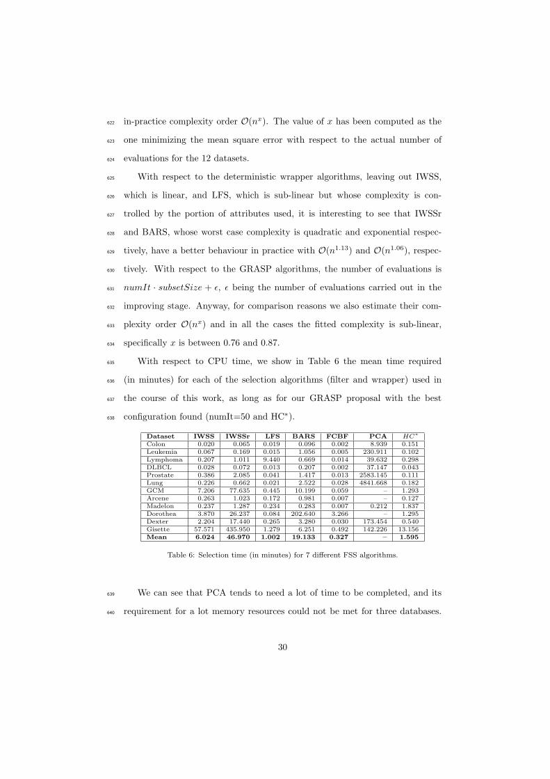
With respect to CPU time, we show in Table 6 the mean time required635

(in minutes) for each of the selection algorithms (filter and wrapper) used in636

the course of this work, as long as for our GRASP proposal with the best637

configuration found (numIt=50 and HC∗).638

Dataset IWSS IWSSr LFS BARS FCBF PCA HC∗

Colon 0.020 0.065 0.019 0.096 0.002 8.939 0.151

Leukemia 0.067 0.169 0.015 1.056 0.005 230.911 0.102

Lymphoma 0.207 1.011 9.440 0.669 0.014 39.632 0.298

DLBCL 0.028 0.072 0.013 0.207 0.002 37.147 0.043

Prostate 0.386 2.085 0.041 1.417 0.013 2583.145 0.111

Lung 0.226 0.662 0.021 2.522 0.028 4841.668 0.182

GCM 7.206 77.635 0.445 10.199 0.059 – 1.293

Arcene 0.263 1.023 0.172 0.981 0.007 – 0.127

Madelon 0.237 1.287 0.234 0.283 0.007 0.212 1.837

Dorothea 3.870 26.237 0.084 202.640 3.266 – 1.295

Dexter 2.204 17.440 0.265 3.280 0.030 173.454 0.540

Gisette 57.571 435.950 1.279 6.251 0.492 142.226 13.156

Mean 6.024 46.970 1.002 19.133 0.327 – 1.595

Table 6: Selection time (in minutes) for 7 different FSS algorithms.

We can see that PCA tends to need a lot of time to be completed, and its639

requirement for a lot memory resources could not be met for three databases.640

30

FCBF is the fastest of all due to its filter nature, but as was seen in Table641

2, it also selects a huge number of attributes. So the two fastest wrapper FSS642

algorithms are LFS and our GRASP proposal which, as Table 4 shows, performs643

better than LFS.644

7. Conclusions and Future Work645

In this paper we have presented a GRASP-based algorithm for feature subset646

selection in high-dimensional datasets. The main goal is to maintain the perfor-647

mance (accuracy and degree of reduction in the number of selected attributes)648

with respect to other state-of-the-art FSS algorithms designed for this problem,649

but with the advantage of needing a significantly smaller number of wrapper650

evaluations. To do this, our GRASP algorithm only uses a small fraction of the651

available attributes in each iteration, which are selected in a pseudo-random652

way, that is, more promising attributes have more chance of being selected. An-653

other novelty lies in the improving stage, which instead of only improving the654

last solution, forces cooperation between all the previously found non-dominated655

solutions by creating a common pool with the variables they contain and running656

an FSS algorithm over them. As a result, we have obtained a highly-competitive657

algorithm for this problem which maintains the performance of state-of-the-art658

deterministic algorithms but in a sub-linear number of wrapper evaluations.659

From the different GRASP instances tested, we recommend the use of those660

running hill climbing or IWSSr in the improving stage.661

An open line of research is to exploit the fact that our algorithm can return662

just one solution, but a set of non-dominated ones. Also, we plan to extend this663

idea to other meta-heuristic algorithms.664

31

Acknowledgments665

This work has been partially supported by the JCCM under project PCI08-666

0048-8577, MEC under project TIN2007-67418-C03-01 and FEDER funds.667

References668

Aha, D. W., Kibler, D., Albert, M. K., 1991. Instance-based learning algorithms.669

Machine Learning 6 (1), 37–66.670

Bermejo, P., Gamez, J., Puerta, J., 2008. On incremental wrapper-based at-671

tribute selection: experimental analysis of the relevance criteria. In: IPMU’08:672

Proceedings of the 12th Intl. Conf. on Information Processing and Manage-673

ment of Uncertainty in Knowledge-Based Systems.674

Bermejo, P., Gamez, J. A., Puerta, J. M., 2009. Incremental wrapper-based675

subset selection with replacement: An advantageous alternative to sequential676

forward selection. In: Proceedings of the IEEE Symposium Series on Com-677

putational Intelligence and Data Mining (SSCI CIDM-2009). pp. 367–374.678

Bishop, C. M., 1995. Neural Networks for Pattern Recognition. Oxford Univer-679

sity Press.680

Blanco, R., Larranaga, P., Inza, I., Sierra, B., 2001. Selection of highly accurate681

genes for cancer classification by estimation of distribution algorithms. In:682

Proceedings of the Workshop of Bayesian Models in Medicine (at AIME-01).683

pp. 29–34.684

Boser, B. E., Guyon, I. M., Vapnik, V. N., 1992. A training algorithm for optimal685

margin classifiers. In: COLT ’92: Proceedings of the fifth annual workshop686

on Computational learning theory. ACM, pp. 144–152.687

32

Cano, J. R., Oscar, C., Fracisco, H., Sanchez, L., 2002. A GRASP algorithm688

for clustering. In: Advances in Artificial Intelligence IBERAMIA 2002. Vol.689

2527 of LNCS. Springer Berlin / Heidelberg, pp. 214–223.690

Casado-Yusta, S., 2009. Different metaheuristic strategies to solve the feature691

selection problem. Pattern Recognition Letters 30 (5), 525–534.692

de Campos, L. M., Fernandez-Luna, J. M., Puerta, J. M., 2002. Local search693

methods for learning bayesian networks using a modified neighborhood in the694

space of dags. In: Advances in Artificial Intelligence IBERAMIA 2002. Vol.695

2527 of LNCS. Springer Berlin / Heidelberg, pp. 182–192.696

Demsar, J., 2006. Statistical comparisons of classifiers over multiple data sets.697

Journal of Machine Learning Research 7, 1–30.698

Duda, R., Hart, P., 1973. Pattern Classification and Scene Analysis. John Wiley699

and Sons.700

Esseghir, M. A., 2010. Effective wrapper-filter hybridization through grasp701

schemata. In: MLR Workshop and Conference Proceedings. Volume 10: Fea-702

ture Selection in Data Mining. pp. 45–54.703

Feo, T. A., Resende, M. G., March 1995. Greedy randomized adaptive search704

procedures. Global Optimization 6 (2), 109–133.705

Feo, T. A., Resende, M. G. C., 1989. A probabilistic heuristic for a computa-706

tionally difficult set covering problem. Operations Research Letters 8 (2), 67707

– 71.708

Festa, P., Resende, M. G., 2010. Effective application of GRASP. In: Lokketan-709

gen, A. (Ed.), Wiley Encyclopedia of Operations Research and Managemente710

Science. Wiley & Sons.711

33

Flores, J., Gamez, J. A., Mateo, J. L., 2008. Mining the esrom: A study of712

breeding value classification in manchego sheep by means of attribute selection713

and construction. Computers and Electronics in Agriculture 60 (2), 167–177.714

Friedman, M., 1937. The use of ranks to avoid the assumption of normality715

implicit in the analysis of variance. Journal of the American Statistical Asso-716

ciation 32, 675–701.717

Garcia, S., Herrera, F., 2008. An extension on ”statistical comparisons of classi-718

fiers over multiple data sets” for all pairwise comparisons. Journal of Machine719

Learning Research 9, 2677–2694.720

Goldberg, D. E., 1989. Genetic Algorithms in Search, Optimization and Machine721

Learning. Addison-Wesley Longman Publishing Co., Inc., Boston, MA, USA.722

Gutlein, M., Frank, E., Hall, M., Karwath, A., 2009. Large-scale attribute se-723

lection using wrappers. In: Symposium on Computational Intelligence and724

Data Mining (CIDM). pp. 332–339.725

Guyon, I., Elisseeff, A., 2003. An introduction to variable and feature selection.726

Journal of Machine Learning Research 3, 1157–1182.727

Hall, M., Frank, E., Holmes, G., Pfahringer, B., Reutemann, P., Witten, I. H.,728

2009. The weka data mining software: an update. SIGKDD Exploration729

Newsletter 11 (1), 10–18.730

Hall, M. A., 1998. Correlation-based feature subset selection for machine learn-731

ing. Ph.D. thesis, University of Waikato, Hamilton, New Zealand.732

Holm, S., 1979. A simple sequentially rejective multiple test procedure. Scandi-733

navian Journal of Statistics 6, 65–70.734

34

Inza, I., Larranaga, P., Etxeberria, R., Sierra, B., 2000. Feature subset selection735

by bayesian network-based optimization. Artifical Intelligence 123 (1-2), 157–736

184.737

Jolliffe, I., 1986. Principal Component Analysis. Springer Verlag.738

Kira, K., Rendell, L., 1992. A practical approach to feature selection. In: 9th739

International Workshop on Machine Learning(ML’92). pp. 249–256.740

Kittler, J., 1978. Feature set search algorithms. Pattern Recognition and Signal741

Processing, 41–60.742

Liu, H., Motoda, H., 1998. Feature Selection for Knowledge Discovery and Data743

Mining. Kluwer Academic Publishers.744

Pudil, P., Novovicova, J., Kittler, J., 1994. Floating search methods in feature745

selection. Pattern Recognition Letters 15 (10), 1119–1125.746

Quinlan, J., 1986. Induction of decision trees. Machine Learning 1, 81–106.747

Resende, M., Ribeiro, C., 2010. Greedy Randomized Adaptive Search Proce-748

dures: Advances, Hybridizations and Applications. In Handbook of Meta-749

heuristics, Chapter 10. Springer.750

Ruiz, R., Aguilar, J. S., Riquelme, J., 2009. Best agglomerative ranked subset751

for feature selection. In: JMLR: Workshop and Conference Proceedings vol.752

4 (New Challenges for feature selection). pp. 148–162.753

Ruiz, R., Riquelme, J. C., Aguilar-Ruiz, J. S., 2006. Incremental wrapper-based754

gene selection from microarray data for cancer classification. Pattern Recog-755

nition 39, 2383–2392.756

Webb, G. I., Boughton, J. R., Wang, Z., 2005. Not so naive bayes: aggregating757

one-dependence estimators. Machine Learning 58 (1), 5–24.758

35

Yang, J., Honavar, V., 1998. Feature subset selection using a genetic algorithm.759

IEEE Intelligent Systems 13 (2), 44–49.760

Yu, L., Liu, H., 2003. Feature selection for high-dimensional data: A fast761

correlation-based filter solution. pp. 856–863.762

36