A Graphical Approach to Solve an Investment Optimization Problem

A Graphical Approach to Solve an InvestmentOptimization Problem

Evgeny R. Gafarov

Ecole Nationale Superieure des Mines, FAYOL-EMSE, CNRS:UMR6158, LIMOS,F-42023 Saint-Etienne, France,

Institute of Control Sciences of the Russian Academy of Sciences,Profsoyuznaya st. 65, 117997 Moscow, Russia,

email: [email protected]

Alexandre Dolgui

Ecole Nationale Superieure des Mines, FAYOL-EMSE, CNRS:UMR6158, LIMOS,F-42023 Saint-Etienne, France


Alexander A. Lazarev

Institute of Control Sciences of the Russian Academy of Sciences,Profsoyuznaya st. 65, 117997 Moscow, Russia,


Frank Werner

Fakultat fur Mathematik, Otto-von-Guericke-Universitat Magdeburg,PSF 4120, 39016 Magdeburg, Germany,


Abstract: We consider a project investment problem, where a set of projectsand an overall budget are given. For each project, a piecewise linear profitfunction is known which describes the profit obtained if a specific amountis invested into this project. The objective is to determine the amount in-vested into each project such that the overall budget is not exceeded and thetotal profit is maximized. For this problem, a graphical algorithm (GrA) ispresented which is based on the same Bellman equations as the best knowndynamic programming algorithm (DPA) but the GrA has several advantagesin comparison with the DPA. Based on this GrA, a fully-polynomial timeapproximation scheme is proposed having the best known running time. Theidea of the GrA presented can also be used to solve some similar schedul-ing or lot-sizing problems in a more effective way, e.g., the related problemof finding lot-sizes and sequencing several products on a single imperfectmachine.

1

1 Introduction

The investment optimization problem can be formulated as follows. A set Nof n potential projects and an investment budget (amount) A > 0 are given.For each project j, j = 1, . . . , n, a profit function fj(t), t ∈ [0, A], is definedin such a way that the value fj(t

′) denotes the profit received if we invest theamount t′ into project j. The goal is to define an amount τj ∈ [0, A]

⋂Z for

each project j ∈ N such that∑n

j:=1 τj ≤ A and the total profit∑n

j:=1 fj(τj)is maximized.

Moreover, for a real-world generalization, it is often necessary to findsuch an optimal solution (investment strategy) for a flexible amount A, i.e.,for all A ∈ [A′, A′′]. So, one looks for an algorithm which is able to solvethis real-world generalization effectively. In the following, we assume that allfunctions fj(t), j = 1, . . . , n, are continuous piecewise linear non-decreasingfunctions (see Fig. 1). If the function fj(t) is defined only for some particularpoints t, e.g., for t1, t2, . . . , tkj with t1 < t2 < . . . < tkj , then we can assumethat fj(t) = fj(ti) holds on the interval [ti, ti+1), i = 1, . . . , kj , where tkj+1 =A. In this paper, we propose an effective pseudo-polynomial algorithm andderive a fully polynomial time approximation scheme (FPTAS) based on it.

To the best of our knowledge, there are no publications on the problemunder consideration. However, there are some close special cases of knapsack-like problems which are as follows.

A special case of the problem is similar to the well-known bounded knap-sack problem [3]:

maximize∑n

j:=1 pjxjs.t.

∑nj:=1wjxj ≤ A,

xj ∈ [0, bj ], xj ∈ Z, j = 1, 2, . . . , n,

(1)

for which a dynamic programming algorithm with a time complexity ofO(nA) is known [3].

The following problem [4] is also similar to the problem under consider-ation:

minimize∑n

j:=1 fj(xj)

s.t.∑n

j:=1 xj ≥ A,

xj ∈ [0, A], xj ∈ Z, j = 1, 2, . . . , n,

(2)

where fj(xj) are piecewise linear as well. For the problem (2), a dynamicprogramming algorithm with a running time of O(

∑kjA) [4] and an FPTAS

with a running time of O((∑

kj)3/ε) [5] are known. A short survey on this

lot-sizing problem can be found in [5] as well.

2

3 10 t

78

25

5 t

2

25

2 4 t

45

25

4 t

1

25

6

4

3

f1f3

f2f4

13

1

2

3

4

Figure 1: Functions fj(t)

3

It is easy to show that the investment optimization problem is NP-hard,since the classical 0-1 knapsack problem is a special case of it.

This problem can be solved by a dynamic programming algorithm (DPA),which is based on the following well-known recursive Bellman equations:

Fj(T ) = maxt=0,1,...,T

{fj(t) + Fj−1(T − t)}, T = A,A− 1, . . . , 1,

with the initial conditions

F0(T ) = 0, for T ≥ 0,F0(T ) = −∞, for T < 0.

(3)

In each stage j, j = 1, . . . , n, a function Fj(T ), j = 1, . . . , n, is calculatedand used in the next stage. Here the value Fj(T ) gives the maximal profitreceived from the realization of the first j projects if a total amount T ≤ Ais invested. Finally, the value Fn(A) denotes the optimal objective functionvalue. Here A and thus all values of T are integer. Note that, if A would berational, we can assign A := �A�.

Usually in a DPA, one works like a calculator, i.e., to calculate Fj(T′),

we consider T ′+1 points t and for each point, we calculate the value fj(t)+Fj−1(T − t). Then we choose the maximal value among these T ′ +1 values.So, the time complexity of such a DPA is O(nA2). Here we do not take intoaccount the analytical form of the functions fj. However, if we work withthe analytical representation (not with particular values fj(t) calculated fort ∈ Z), we will have some advantages.

The remainder of the paper is as follows. In Section 2, we present thegraphical algorithm (GrA) and discuss its advantages in comparison withthe DPA. In Section 3, we illustrate the algorithm on a numerical example.Some advantages of the GrA in comparison with the DPA are discussed inSection 4. In Section 5, we give a modification of the GrA and derive anFPTAS. In Section, 6 a GrA and an FPTAS for a related problem denotedas P-Cost are presented.

2 Graphical Algorithm

Next, we present the graphical algorithm (GrA) which uses the sameBellman equations as the DPA, but considers analytical expressions of thefunctions. We note that the foundations of such a type of algorithm havebeen given e.g. in [1]. The given functions fj(t), j = 1, 2, . . . , n, can be

4

saved in the computer memory in a tabular form as given in Table 1:

Table 1: Function fj(t)

K 1 2 . . . kj

interval K [t1j , t2j ) [t2j , t

3j) . . . [t

kjj , A)

bKj b1j b2j . . . bkjj

uKj u1j u2j . . . ukjj

In Table 1, K denotes the number of the current interval, whose valuesrange from 1 to kj (where the number of intervals kj is defined for each j =1, 2, . . . , n), [tKj , tK+1

j ) is the Kth interval, and bKj , uKj are the parameters ofthe linear function fK

j (t) defined on the kth interval. This data means thefollowing. For each above interval, we store the parameters bKj and uKj fordescribing the function fj(t) = fK

j (t) = uKj · (t− tKj ) + bKj on this interval.For the example given in Fig. 1, the function f1(t) can be presented as

follows:

Table 2: Function f1(t)

K 1 2 3 4

interval K [0, 3) [3, 10) [10, 13) [13, 25]

bK1 0 0 7 8

uK1 0 1 13 0

The points t1j , t2j , . . . , t

kjj are called "break points" since the slope of the

function changes at these points. The functions Fj(T ) can be presented inthe same way.

First, we formally describe the graphical algorithm (GrA). In the fol-lowing, we denote the starting points as SP and the counter of the currentinterval as CI.

Step I. j := 1. Copy the table for the function f1(t) into the table for thefunction F1(T ).

Step II.a Let j > 1 and assume that the function Fj−1(T ) is known for allresulting intervals given in Table 5. Assign SP := A and CI := 1;

Table 5: Function Fj−1(T )

5

K 1 2 . . . BPj

interval K [TBPj+1, TBPj ) [TBPj , TBPj−1) . . . [T2, T1)

bK b1 b2 . . . bBPj

uK u1 u2 . . . uBPj

Step II.b Calculate the intervals of the reflected function f ′j(t) = fj(A− t).

Table 6: Intervals of the reflected function f ′j(t)

K 1 2 . . . kj

interval K [t2, t1) [t3, t2) . . . [0, tkjj )

Here t1 = SP , and the other points tK are calculated as follows:tK = tK−1 − (tK+1

j − tKj ), K = 2, . . . , kj . On the interval [tK+1, tK), wehave f ′

j(t) = bK+1j − uKj (t− tK+1), where f ′

j(t) is the reflected function.

Step II.c For each point TK and each point tK , calculate their equations.An equation for a point denotes the values which are used to calculateFj(T ), where T belongs to the interval [SP − ε, SP ].

To calculate the equation for a point TK , we have to find the interval[ts+1, ts), where Tk ∈ [ts+1, ts). The equation for this point is f ′

j(TK) +Fj(TK) − usj · ε. In the same way, we calculate the equation for tK . LettK ∈ [Tr, Tr+1). Then we have the equation f ′

j(tK) + Fj(tK)− ur · ε.We consider only points TK < SP and points tK > 0.

Step II.d Among all equations, we have to find a leading equation, i.e., aleading point. Let us consider the two points x1 and x2 and their equationsBx1 − Ux1ε and Bx2 − Ux2ε. If Bx1 > Bx2 or (Bx1 = Bx2 and Ux2 > Ux1),then the point x1 dominates the point x2. For the leading point, there is noother point which dominates it.

Step II.e Calculate the length of the minimal interval LMI =min{ts − Tr}, s = 1, . . . , kj , r = 1, . . . , BPj−1, where ts > Tr. Nowwe check whether there is a point x′ with an equation Bx′ − Ux′

ε, which isdominated by the leading point x∗ and whose diagram has an intersectionon the interval [SP − LMI, SP ]. Let SP − ε′ be an intersection point. Wehave to find the minimal value ε′ among all such points x′. Let εmin besuch a point. Then LMI := εmin. Such points SP − LMI will be called

6

intersection points.

Step II.f In the table for the function Fj(T ), save a column with the interval[tCI , tCI+1] = [SP − LMI, SP ] and the values bCI = Bx∗ − Ux∗ · LMI,uCI = Ux∗ .

Step II.g If the slope of the function on the interval of Fj(T ) just savedbefore was the same, then we can join both intervals.

Step II.h SP := SP − LMI and CI := CI + 1. If SP > 0, then GOTOStep II.b.

Step III. Modify the form of the table for the function Fj(T ) into the formas in Table 5. Let j := j + 1. If j ≤ n, GOTO Step II.a.

Step IV. Use backtracking to find an optimal solution at the point A andthe optimal objective function value Fn(A).

End of the Algorithm

Lemma 1 At each stage of the algorithm, there are no more than BPj +kj + kj · BPj intersection points.

Proof: During step 2, there are no more than kj · BPj different equations(with different points or different slopes). At each point (SP −LMI) calcu-lated according to the points TK and tK , only for two points the equations(slopes of their equations) are changed. In the initial point T = A, we haveonly BPj + kj equations. All these equations correspond to linear functions.So, there are no more than BPj + kj + k ·BPj intersection points.

�

Theorem 1 The GrA constructs an optimal solution for all points T ∈[0, A] in O(n(BPmaxkmax)

2) time, where BPmax = maxl=1,2,...,n{BPj},kmax = maxj∈N kj.

Proof: Since the GrA uses the same Bellman equations as the DPA, itfounds an optimal solution for any T ∈ [0, A].

Steps II.b− II.e can be simultaneously performed in O(BPj + kj) timefor each SP . The number of starting points SP is less than BPj ·kj+(BPj+kj+kj ·BPj), where the number of intersection points is BPj+kj+kj ·BPj .

7

Since there are n stages, the time complexity of the algorithm is equal toO(n(BPmaxkmax)

2).�If we only need to find an optimal solution for T ∈ [0, A], T ∈ Z,

then the GrA can be modified as follows. If in the table for the functionFj(T ), j = 1, 2, . . . , n, we have two columns with the intervals [TK−1, TK)and [TK , TK+1), where TK /∈ Z, then we can change the intervals to[TK−1, �TK�) and [�TK, TK+1). If ts ∈ (�TK�, �TK) at the next stage,then its equation is not taken into account. Thus, we have BPmax ≤ A andobtain the following corollary. Denote this modification as GrA-I.

Corollary 1 The GrA-I constructs an optimal solution for all points T ∈[0, A], T ∈ Z, in O(n(A · kmax)

2) time, where kmax = maxj∈N kj .

2.1 A Modification of the GrA-I with Time ComplexityO(nkmaxA log(kmaxA))

Steps II.b − II.e can also be performed in another way. At each step II (ifan intersection point is not considered), only two equations go out and twonew equations go in. In step 1 (or at the first iteration of step II, but not I !)(when SP = A) of each stage j, j = 2, . . . , n, we can sort all BKj−1+kj firstequations in non-decreasing order of the time points t, when they becomeleading equations. So, the first equation in this ordered list is the leadingone. This ordering can be done in O((BKj−1 + kj) log(BKj−1 + kj)) time.To find an intersection point εmin, we only need to compare the first andsecond equations in this list. To add two new equations in a step of theGrA, we only need to perform O(log(BKj−1 + kj)) operations (to put theminto the ordered list). Below we explain such a technique for Stage 3 of thenumerical example considered.

In the same way, we can create a list of the lengths of the intervalswhich are used to compute LMI. In each step, the length of the list of theLMI values is less than or equal to kj . So, to construct this list, we needto perform O(kj log(kj)) operations. To recalculate it, we need O(log kj)operations in each step. The first value in the list is LMI.

So, instead of O(BKj · kj) operations in each step i > 1, we need only toperform O(log(BKj−1 + kj)) operations and O((BKj−1 + kj) log(BKj−1 +kj)) operations in the first step. Therefore, the time complexity of the mod-ified GrA-I is O(nkmaxA log(kmaxA)), if we only need to find a solution forany T ∈ [0, A], T ∈ Z.

8

3 Numerical Example

In this section, the idea of the GrA is explained on the numerical examplepresented in Fig. 1, where n = 4.

Stage 1. Determination of F1(T ).

It is obvious that F1(T ) = f1(t).


Step 1.Let us analyze Fig. 2.1. To calculate the value F2(25) in the DPA, we

can do the following. We draw F1(T ) and f2(t) as shown in the figure, wheref2(t) is drawn in a reflected way from the point t, i.e., the diagram of functionf ′2(t) = f2(25 − t) is drawn. Now, for each t ∈ [0, 25], it is easy to calculate

the values f2(t)+F1(25− t). The diagram of this function is presented by adotted line. We note that the diagram of the function f2(t) + F1(25 − t) ispiecewise linear and continuous as well. So, its maximal values are reachedat the break points, which correspond to the break points of the functionsF1(T ) and f2(t), i.e., t1, t2, T2, T3, T4, T5. We have the maximal value 10 atthe point t = 20 which corresponds to the break point t2.

To calculate the values F2(25 − ε), we have to shift the diagram of thefunction f2(t) (and all break points t1, t2 which correspond to function f2(t))to the left by ε. It is easy to see that the value at the new break point t2will be 10 − u41ε = 10, if ε ≤ t2 − T2 = 20 − 13 = 7. Here u41 is the slope ofthe function F1(T ) on the interval [T2, A). At the same time, the values atthe other break points will be changed as follows:F ′(T5) = F1(T5)− ε ∗ u22 = 2,F ′(T4) = F1(T4)− ε ∗ u22 = 2,F ′(T3) = F1(T3)− ε ∗ u22 = 9,F ′(T2) = F1(T2)− ε ∗ u22 = 10,F ′(t1) = F1(t1)− ε ∗ u41 = 8.

Here F ′(Tx) denotes the equality corresponding to the point Tx if we shiftthe diagram of the function f2(t) to the left. So, on the interval [25−7, 25] =[18, 25], we have F2(T ) = 10− u41ε = 10 (see Fig. 2.2).

Step 2.At the point T = 18, the linear part of F1(T ) corresponding to the break

point t2 changes. We have the equation: F ′(t2) = F1(t2 = 18) − ε · u31 =10 − ε · 1

3 (see Fig. 2.3). The same change happens for the point T2. For

9

3 10 t

78

25

F1

f213 20

3 10 t

78

25

F2

13 18

3 10 t

78

25

F2

13

3 10 t

78

25

F2

13 18

15

3 10 t

78

25

F2

13 15

3 10 t

78

25

F2

13 15

1

2

3 6

5

4

t1

t2

T2T3

T4

t1

t1

t1

t1t1

t2

t2

t2

t2t2

T5

Figure 2: Function F2(T )

10

T = 18− ε, we obtain the values F ′(T2) = 10− ε · u12 = 10− ε25 . The slopesof all other functions F ′(T3), F

′(T4), F′(T5), F

′(t1) do not change. So, thepoint t2 remains the leading point.

Subsequently, we will use the following two terms: a leading equation anda leading point. Let us consider the two points x1 and x2 and their equationsBx1 − Ux1ε and Bx2 − Ux2ε. If Bx1 > Bx2 or (Bx1 = Bx2 and Ux2 > Ux1),then the point x1 dominates the point x2. For a leading point, there is noother point which dominates it.

We continue with shifting the diagram of the function f2(t) to the leftfrom the point t = 18. The values F2(18− ε) are calculated as F2(18− ε) =10 − ε13 corresponding to an equation for the point t2. This holds till thenext change of a slope which happens at the point t = 15, where t2 and T3

meet each other. So, on the interval [15, 18], we have F ′2(t) = 10− (18− t)13

(see Fig. 2.4).

Step 3.From the point T = 15, we have the equation: F ′(t2) = F (t2)− ε · u21 =

10− 3 · 13 − ε · 1 = 9− ε. The change of an equation happens for the point T3

as well. For T = 15 − ε, we obtain the values F ′(T3) = 9 − ε · u12 = 9 − ε25 .So, the point T3 becomes a leading one, since its slope is less and it startsfrom the same value 9 as the point t2.

We continue with shifting the diagram of the function f2(t) to the leftfrom the point t = 15. The values F2(15− ε) are calculated as F2(15− ε) =9−ε25 which corresponds to the equation for the point T3. This holds till thenext change of a slope (where the point t1 and T2 meet each other), namelyat the point t = 13. So, on the interval [13, 15], we have F2(t) = 9−(15− t)25(see Fig. 2.5).

We continue our calculations in the same way. For each of the k2 +BP1

break points, where BP1 is the number of break points of the function F1(T )),we have an equation which characterizes how the value F2(T ) will changeif we shift the diagram of the function f2(t) to the left (i.e., those valuesof the function F2(T ) we will have). Among these k2 + BP1 points, wechoose the leading one and according to its equation we calculate F2(T ).This calculation holds till the next point t, where a break point of f2(t) anda break point of F1(T ) will meet each other.

In such a way, we obtain:

Step 4. For t ∈ [10, 13]: F2(t) = 815 − (13 − t) · 2

5 and the leading point T3

the equation of which is F ′(T3) = 815 − ε · u22 = 81

5 − ε · 25 .

Step 5. For t ∈ [5, 10]: F2(t) = 7− (10 − t) · 1 and the leading point t2 the

11

equation of which is F ′(t2) = 7− ε · u21 = 7− ε.

Step 6. For t ∈ [0, 5]: F2(t) = 2 − (5 − t) · 25 and the leading point T4 the

equation of which is F ′(t2) = 2− ε · u22 = 2− ε · 25 .

The final diagram of the function F2(T ) is presented in Fig. 2.6, and itslinear parts are described in Table 3.

Table 3: Function F2(t)

K 1 2 3 4 5

interval K [0, 5) [5, 10) [10, 15) [15, 18) [18, 25)

bK 0 2 7 9 10

uK 25 1 2

513 0


Next, we describe how the function F3(T ) is calculated using thefunctions F2(T ) and f3(t). All steps are performed in the same way as forthe stage 2. We present only their short description. In the following tables,a point (x, y) is described in the form x|y.

Step 1. Starting point T = 25, see Fig. 3.1.

t1 : 0|10 t4 : 0|15∗ T4 : 0|12t2 : 0|10 T2 : 0|15 T5 : 0|7t3 : 0|14 T3 : 0|14 T6 : 0|5

This data means the follows. The point t1 takes part in calculatingthe values F3(T ) according to the equation 10 − ε · 0. In the table, aleading point where only one equation influences F3(T ) is marked bythe symbol ∗. The length of the minimal interval (LMI) is obtained asLMI = t4 − T2 = 1, i.e., on this interval, the slopes of the equations donot change, which means that all the points hold their equations. So, onthe interval [25 − LMI, 25] = [24, 25], the slope of the function F3(T ) isequal to the slope of the equation for the point t4, i.e., 0. In addition, wecalculate F3(25) = 10 + 5 = 15.


12

5 10 t

7

9

25

F2

15 18

1

10

T2T3

T4

T5

T6f3 t1t2

t3

t4

15

5 10 t

7

9

25

F2

15 18

2

10

T2T3

T4

T5

T6f3 t1t2

t3

t4

15

5 10 t

7

9

25

F2

15 18

3

10

T2T3

T4

T5

T6f3 t1t2

t3

t4

15

5 10 t

7

9

25

F2

15 18

5

10

T2T3

T4

T5

T6f3 t1t2

t3

t4

15

5 10 t

7

9

25

F2

15 18

4

10

T2T3

T4

T5

T6f3 t1t2

t3

t4

15

F3


13

– t4 :13 |15∗ –

– T2 :12 |15 –

– – –

Next, we only present the calculations made in essential steps of thealgorithm.


– t4 : 1|12 T4 :12 |12∗

t2 =25 |83

5 T5 : 0|7t3 :

25 |114

5 T3 : 0|9 –

We have LMI = t3 − T4 = 12 − 10 = 2. We check whether the equationfor the point t3 becomes leading on the interval [14, 16] (i.e., whether itovercomes the equation for T4):

−1

2ε+ 12 = −2

5ε+ 11

4

5;

1

5=

1

10ε; ε = 2.

This means that LMI = 2 = ε, and T4 remains the leading point on thewhole interval [14, 16]. On the interval [14, 16], the slope of the functionF3(T ) is equal to 1

2 .


t1 : 1|7 t4 :25 |63

5 T4 is out of ranget2 : 1|5 T5 :

12 |61

2

t3 : 1|7∗ –

We have LMI = t3 − T5 = 1. We check whether the equation for thepoint t4 becomes leading on the interval [9, 10] (i.e., whether it overcomesthe equation for t3):

−ε+ 7 = −2

5ε+ 6

3

5;

2

5=

3

5ε; ε =

2

3.

On the interval [913 , 10], the slope of the function F3(T ) is equal to 1.


t1 :25 |13

5

t2 :25 |45

t3 is out of range T6 : 2|4

14

We have LMI = t2 − T6 = 2. However, there is an intersection point of theequations of the points T6 and t1:

−2ε+ 4 = −2

5ε+ 1

3

5;

12

5=

8

5ε; ε =

3

2.

So, on the interval [212 , 4], the slope of the function F3(T ) is equal to 2.

Step 18. Starting point T = 212 , see Fig. 3.5.

In this step, the leading point is t1. Thus, on the interval [0, 212 ], the slope

of the function F3(T ) is equal to 25 .

The final diagram of the function F3(T ) is presented in Fig. 3.5, and itslinear parts are described in Table 4.

Table 4: Function F3(t)

K 1 2 3 4 5 6 7 8

interval K [0, 212 ) [21

2 , 4) [4, 913 ) [91

3 , 14) [14, 16) [16, 21) [21,24) [21,25)bK 0 1 4 61

3 11 12 14 15

uK 25 2 2

5 1 12

25

13 0


Next, we describe how the function F4(T ) is calculated using the func-tions F3(T ) and f4(t). In the case of a step function f4(t), we can performthis stage in an easier way. We can construct the functions Φ1(T ) = F3(T ),Φ2(T ) = 1 + F3(T − 3) and Φ3(T ) = 4 + F3(T − 4). Then we have to con-struct the function F4(t) = max{Φ1(T ),Φ2(T ),Φ3(T )}. All these functionsare presented in Fig. 4.

Of course, we can perform the same operations like at Stages 2 and 3,but this is more complicated and takes more time.

Backtracking.To find an optimal solution at the point T = 25, we can do backtracking.

We have τ4 = 4 and f4(τ4) = 4, τ3 = 6 and f3(τ3) = 5, τ2 = 5 and f2(τ2) = 2;τ1 = 10 and f1(τ1) = 7. Moreover, F ∗(25) = 18.

Let us analyze the running times of the graphical algorithm (GrA) andthe DPA. In the DPA, we have to consider (4 − 1) ∗ 25(25+1)

2 + 25 = 1000points t.

15

t25

F3 115

18

t25

F4

218


16

In the first stage of the GrA, we consider 4 points of the function f1(t). Atthe second stage, we consider less than 4 ∗ 2 = 8 steps and recalculate up to4+2 = 6 equations in each step (practically, we have 6+6+6+5+4+3+2 =32). At the second stage, we consider less than the 5∗4 = 20 steps obtainedfrom the break points and the two steps obtained due to the intersection ofequations (practically, 17 steps) and recalculate up to 5+4 = 9 equations ineach step (practically, we have 9+9+9+9+8+8+8+3∗7+4∗6+5+4+3+2 =119). In the last step, we have to consider 3 ∗ 8 = 24 break points of thethree functions Φ1(T ),Φ2(T ),Φ3(T ). Thus, in the GrA, we consider up to4+32+119+24 = 179 points or equations. If we scale our instance to a bignumber M (i.e., we multiply all input data by M), then the running time ofthe DPA increases M2 times, but the running time of the GrA remains thesame. Of course, for each equation, we have to do some simple calculations(operations). However, this number is constant: O(1).

Stage 3 of the Numerical Example for the Modification of the GrA

In Fig. 5.1, the diagrams of F ′(t1), F ′(t2), F ′(t3), F ′(t4), F ′(T1),F ′(T2), F

′(T3), F′(T4), F

′(T5), F′(T6) are presented. So, the ordered list in

step 1 of the stage is (t4, T2, T3, t3, T4, t1, t2, T5, T6).In step 2, we delete the two equations corresponding to t4 and T2 from

the list. To enter a new equation F ′(t4), we do the following. Compare F ′(t4)and F ′(t1). Their intersection point is (9, 10), i.e., t = 9, F = 10. Moreover,at SP = 24, the value of F ′(t4) is larger. So, in the list, t4 is before t1. Thencompare it with t3. The intersection point is (21, 14) and the value of F (t4)is larger at SP . Finally, we compare it with T3. We have t4 before T3 in thelist. Analogously, we look for a position for T2 in the list. The ordered listremains the same (t4, T2, T3, t3, T4, t1, t2, T5, T6). In Fig. 5.2, the diagramsof the corresponding equations in step 2 are shown.

To be exact, we have to save not the points tx and Tx in the list but thepairs (Intervalx, tx), where Intervalx is the interval where the equation txis leading. In step 3, we delete the two old equations corresponding to t4and T3 from the list and insert two new equations corresponding to thesepoints. We have the following order: (t4, T3, t3, T2, T4, t1, t2, T5, T6) (see Fig.5.3). We note that T2 dominates T4 only before the point t = 21, i.e., on theinterval [21, 22). This information has to be saved in the list.

Analogously, in step 4, we have the same order(t4, T3, t3, T2, T4, t1, t2, T5, T6). We remind that T4 dominates T2 fort < 21.

17

t25

F’(t ), F’(T )4

115 2

F’(t ), F’(T )3 3

F’(T )4

F’(t ), F’(T )1 2

F’(T )5

F’(T )6

t25

F’(t )4

215

F’(t ), F’(T )3 3

F’(T )4

F’(t ), F’(T )1 2

F’(T )5

F’(T )6

F’(T )2

t25

F’(t )4

315

F’(T )3

F’(T )4

F’(t ), F’(T )1 2

F’(T )5

F’(T )6

F’(T )2

F’(t )3

t25

F’(t )4

415

F’(T )3

F’(T )4

F’(t ), F’(T )1 2

F’(T )5

F’(T )6

F’(T )2F’(t )3

Figure 5: List of equations in stage 3

18

We have to mention as well that after deleting an equation tx from thelist, we have to reinsert (reorder) the equations of its left and right neigh-bors as well, since it has common intersection points (edges of the intervalIntervalx). This means that in each step, we have to delete up to 6 equationsfrom the list and to add 6 new equations.

4 Some Benefits of the GrA (GrA-I) in Comparisonwith the DPA

1. The time complexity of the modified GrA-I is O(nkmaxA log(kmaxA))in contrast to the time complexity O(nA2) of the DPA.

2. In spite of the fact that the complexity of the non-modified GrA-I isO(n(A ·kmax)

2) and the complexity of the DPA is O(nA2), we supposethat in practice, the running time of the GrA-I is substantially less.This conjecture is made based on our numerical results with graphicalalgorithms for other problems.

3. The running time of the GrA for two instances I1 and I2, where allparameters of I2 are equal to the parameters of I1 multiplied by M >1, M ∈ Z, will be the same, although the running time of the DPAincreases M2 times. Thus, using the GrA, we can solve large scaleinstances or instances with real numbers in a more effective way.

4. If at stage j, j = 1, 2, . . . , n, we have kjBPj > A, then we can recalcu-late the table for Fj(T ) from the table used in the DPA and continuewith all other stages according to the DPA. This means that the run-ning time of such a modification is always less than the running timeof the DPA.

5. The GrA-I is more effective for some sub-cases. As we saw in Section 2for a numerical instance, for some functions at stage 4, the complexityof the GrA-I will be less, if all functions fj(t) are step functions. Thenthe time complexity of the GrA-I is O(nkmaxA), which is substantiallyless than the complexity of the DPA considered.

6. As it is shown in Section 5, it is easier to construct an FPTAS basedon a GrA.

19

5 An FPTAS Based on a GrA

In this section, a fully polynomial-time approximation scheme (FPTAS) ispresented based on the corresponding GrA.

First, we recall some relevant definitions. For the optimization problemof minimizing a function F (π), a polynomial-time algorithm that finds afeasible solution π′ such that F (π′) is at most ρ ≥ 1 times less than theoptimal value F (π∗) is called a ρ-approximation algorithm; the value of ρis called a worst-case ratio bound. If a problem admits a ρ-approximationalgorithm, it is said to be approximable within a factor ρ. A family of ρ-approximation algorithms is called a fully polynomial-time approximationscheme, or an FPTAS, if ρ = 1 + ε for any ε > 0 and the running time ispolynomial with respect to both the length of the problem input and 1/ε.Notice that a problem, which is NP-hard in the strong sense, admits noFPTAS unless P = NP.

Let LB = maxj=1,...,n

fj(A) be a lower bound and UB = n ·UB be an upper

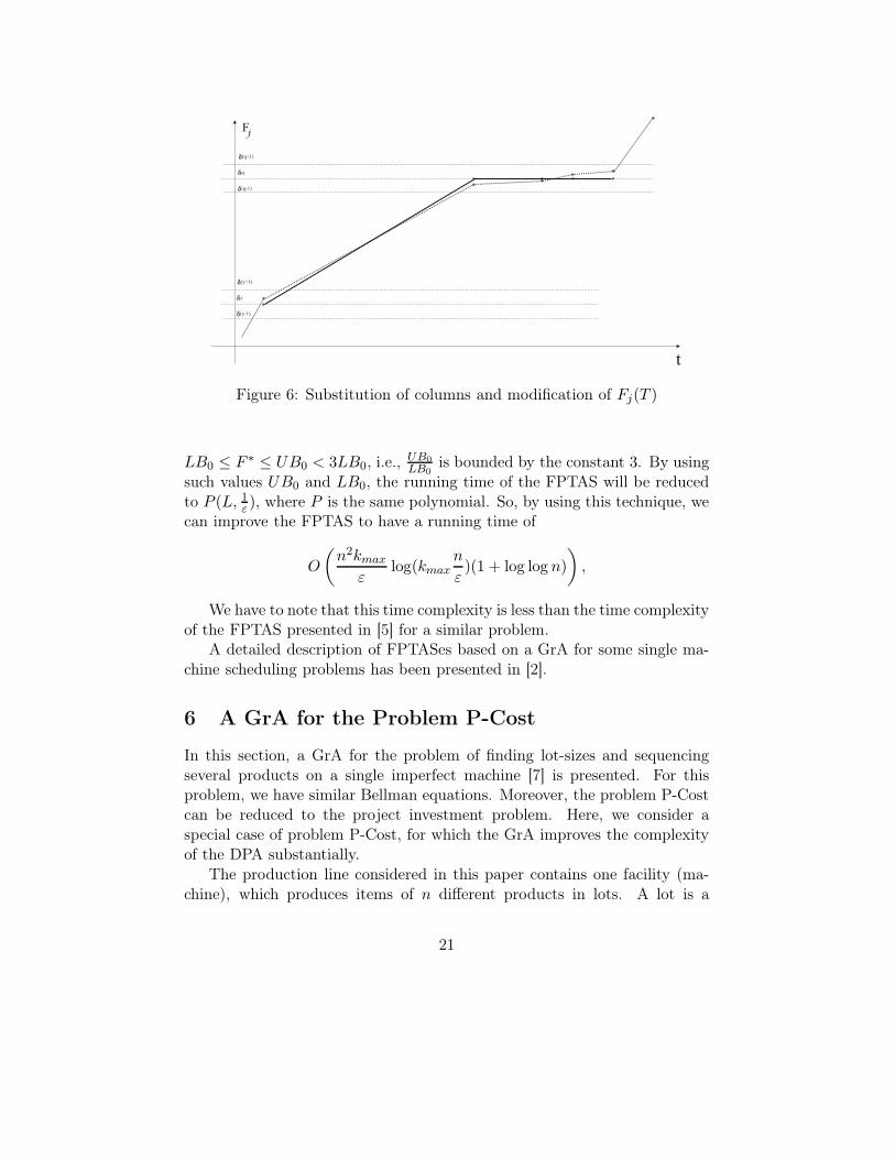
bound on the optimal objective function value for the problem.The idea of the FPTAS is as follows. Let δ = εLB

n . To reduce thetime complexity of the GrA, we have to diminish the number of columnsBKj considered, which is the number of different objective function values0 = b1 = b2, b3, . . . , bBLk = UB. If we do not consider the original valuesbk but the values bk which are rounded up or down to the nearest multipleof δ values bk, there are no more than UB

δ = n2

ε different values bk. Thenwe will be able to convert the table for the function Fj(t) into a similartable with no more than 2n2

ε columns (see Fig. 6). Furthermore, for such amodified table (function) F ′(t), we will have |F (t) − F ′(t)| < δ ≤ εF (π∗)

n . Ifwe do the rounding and modification after each step III of the GrA, then thecumulative error will be no more than nδ ≤ εF (π∗), and the total runningtime of the n runs of the GrA will be

O

(n3kmax

εlog(kmax

n2

ε)

),

i.e., an FPTAS is obtained.In [6], a technique was proposed to improve the complexity of an ap-

proximation algorithm for optimization problems. This technique can bedescribed as follows. If there is an FPTAS for a problem with a run-ning time bounded by a polynomial P (L, 1ε ,

UBLB ), where L is the length

of the problem instance and UB, LB are known upper and lower bounds,and the value UB

LB is not bounded by a constant, then the technique en-ables us to find in P (L, log log UB

LB ) time values UB0 and LB0 such that

20

Fj

t

( )q+1

q

( )q-1

( )y 1+

y

( )y 1-

Figure 6: Substitution of columns and modification of Fj(T )

LB0 ≤ F ∗ ≤ UB0 < 3LB0, i.e., UB0LB0

is bounded by the constant 3. By usingsuch values UB0 and LB0, the running time of the FPTAS will be reducedto P (L, 1ε ), where P is the same polynomial. So, by using this technique, wecan improve the FPTAS to have a running time of

O

(n2kmax

εlog(kmax

n

ε)(1 + log log n)

),

We have to note that this time complexity is less than the time complexityof the FPTAS presented in [5] for a similar problem.

A detailed description of FPTASes based on a GrA for some single ma-chine scheduling problems has been presented in [2].

6 A GrA for the Problem P-Cost

In this section, a GrA for the problem of finding lot-sizes and sequencingseveral products on a single imperfect machine [7] is presented. For thisproblem, we have similar Bellman equations. Moreover, the problem P-Costcan be reduced to the project investment problem. Here, we consider aspecial case of problem P-Cost, for which the GrA improves the complexityof the DPA substantially.

The production line considered in this paper contains one facility (ma-chine), which produces items of n different products in lots. A lot is a

21

maximal set of items of the same product manufactured sequentially on themachine. The machine cannot process more than one item simultaneously.A sequence-dependent setup time is required between items of different prod-ucts. The machine is imperfect in the following two senses: it can producedefective items which are not repairable, and it can break down. It is as-sumed that no item can be produced during a setup or breakdown and thatsetup and breakdown times cannot overlap. The following deterministic pa-rameters are assumed to be given for each product j, j = 1, . . . , n: bj , bj > 0,is the demand for good quality items; cj, cj > 0, is the per item cost of theunsatisfied demand; tj, tj > 0 is the processing time of an item; si,j, si,j ≥ 0is the setup time between items of products i and j; ϕj(x) is a non-decreasinginteger-valued function representing the number of defective items, x is thetotal manufactured quantity of product j; fj(0) = 0, and fj(x) < x forx = 1, 2, . . . , n; T (x1, . . . , xn) is a non-negative non-decreasing real-valuedfunction representing the cumulative machine breakdown time before theproduction of the last item, and xj is the total number of manufactureditems of product j.

The problem is to minimize the total cost

n∑j:=1

cj max{0, bj − (xj − fj(xj))},

of demand dissatisfaction subject to the constraint that the completion timeCmax of the last item does not exceed a given upper bound A. This problemwas denoted as P-Cost.

In [7], this problem is solved in two steps. In the first step, a sequenceof lots is computed by using an exact B&B algorithm for the TravelingSalesman Problem to minimize total setup time. The time complexity ofthis algorithm is O(n22n). Let TT be the total time given for production.Then A = TT − TS∗, where TS∗ is the minimal total setup time.

In the second step, the function

F (x1, . . . , xn) =

n∑j:=1

cj max{0, bj − (xj − fj(xj))}

is minimized, where∑n

j:=1 xjtj ≤ A. It is obvious that this problem can besolved in O(nA2) time by a DPA with Bellman equations similar to the onespresented in Section 1.

In [7], the authors considered a special case of this problem, wherefj(xj) = �αjxj�, and they presented an FPTAS with a time complexity

22

of

O

⎛⎝n3

ε2+ n3 log log(

n∑j:=1

cjbj)

⎞⎠ .

According to the results of the numerical experiments provided in [8], thisFPTAS works slower than an exact algorithm provided by CPLEX for a MIPformulation of the problem. However, we have to note the following. Sincethe traveling salesman problem (TSP) solved in the first step is many timesmore difficult, it seems to be necessary to do the following. First, using aneffective algorithms we find UBTS and LBTS , which are an upper and a lowerbound on the optimal objective function value for the TSP. Then we use theDPA to solve the problem P-Cost, where A = TT − LBTS . As a result ofthe DPA, we will have optimal solutions for all A′ ∈ [0, A], in contrast to thefact that CPLEX provides only an optimal solution for A′ = A. Then wereturn to the TSP and decide whether it makes sense to continue the B&Bcalculations, i.e., which result will be obtained for the problem P-Cost, ifwe improve the current value UBTS . So, this approach seems to be moreeffective than a combination of the B&B algorithm for the TSP and CPLEX.

If we assume fj(xj) = αjxj, then we can use the GrA to solve theproblem, where kj = 2, j = 1, . . . , n. The analytical form fj(xj) = αjxjseems to be more adequate than fj(xj) = �αjxj� since, in practice, we dealwith functions fj(xj) statistically received.

Lemma 2 The problem P-Cost with fj(xj) = αjxj, j = 1, . . . , n, is NP-hard.

Proof: We present a polynomial time reduction from the partition problem,which is as follows.Partition problem. A set N = {a1, a2, . . . , an} of values a1 ≥ a2 ≥ . . . ≥an > 0 with ai ∈ Z+, i = 1, 2, . . . , n, and a value A ∈ Z, A = 1

2

∑nj=1 aj are

given. Is there a subset N ′ ⊂ N such that∑

j∈N ′ aj = A?Each lot j ∈ N corresponds to an item j ∈ N . Moreover, we have

bj = 1, αj = 0, cj = tj = aj and A = A. There exists an optimal solutionof the problem P-Cost with F ∗ = A if and only if there exists such a subsetN ′ for the partition problem. �

Theorem 2 The problem P-Cost with fj(xj) = αjxj , j = 1, . . . , n, can besolved by the GrA-I in O(nA logA) time.

23

Theorem 3 For the problem P-Cost with fj(xj) = αjxj, j = 1, . . . , n, thereexists an FPTAS based on the GrA with a time complexity of

O

⎛⎝n2

εlog(n/ε) + n2 log log(

n∑j:=1

cjbj)

⎞⎠ .

7 Concluding Remarks

The graphical approach can be applied to problems, where a pseudo-polynomial algorithm exists based on the Bellman equations. For the in-vestment optimization and the P-Cost problems, the graphical algorithmimproved the complexity of the corresponding pseudo-polynomial algorithmsubstantially. An FPTAS based on this GrA can be constructed with thebest running time among the FPTASes known.

References

[1] Lazarev, A.A. and Werner, F.: A Graphical Realization of the Dy-namic Programming Method for Solving NP-hard Problems. Computers& Mathematics with Applications. Vol. 58, No. 4, 2009, 619 – 631.

[2] Gafarov, E.R.; Dolgui, A. and Werner F.: Dynamic Programming Ap-proach to Design FPTAS for Single Machine Scheduling Problems. Re-search Report LIMOS UMR CNRS 6158 (2012).

[3] Kellerer, H.; Pferschy, U. and Pisinger, D.: Knapsack Problems,Springer-Verlag, Berlin, 2004.

[4] Shaw, D.X. and Wagelmans, A.P.M.: An Algorithm for Single-Item Ca-pacitated Economic Lot Sizing with Piecewise Linear Production Costsand General Holding Costs, Management Science, Vol. 44, No. 6, 1998,831–838.

[5] Kameshwaran, S. and Narahari, Y.: Nonconvex Piecewise Linear Knap-sack Problems, European Journal of Operational Research, 192, 2009,56–68.

[6] Chubanov, S.; Kovalyov, M.Y. and E. Pesch: An FPTAS for a Single-Item Capacitated Economic Lot-Sizing Problem with Monotone CostStructure, Math. Program., Ser. A 106 (2006) 453 – 466.

24

[7] Dolgui, A.; Kovalyov, M.Y. and Shchamialiova, K.: Multi-Product Lot-Sizing and Sequencing on a Single Imperfect Machine, Comput. Optim.Appl., Vol. 50 (2011) 465 – 482.

[8] Schmeleva, K.; Delorme, X.; Dolgui, A.; Grimaud, F. and Kovalyov,M.K.: Lot-Sizing on a Single Machine, ILP Models, Computers andIndustrial Engineering, Vol. 65 (2013) 561 – 569.

25

A Graphical Approach to Solve an Investment Optimization Problem

Documents